Clustering: Evolutionary Approaches - Alexandru Ioan Cuza ...pmihaela/thesis... · University...
178
University “Alexandru Ioan Cuza” of Iasi, Romania Faculty of Computer Science Clustering: Evolutionary Approaches PhD Candidate Mihaela Elena Breaban Supervisor Prof. PhD Henri Luchian Thesis committee Prof. PhD Dan Dumitrescu, Babes-Bolyai University, Cluj-Napoca, Romania Prof. PhD Dan Simovici, University of Massachusetts at Boston, USA Prof. PhD Daniela Zaharie,West University of Timisoara, Romania A thesis submitted to “Alexandru Ioan Cuza” University for the degree of Philosophiæ Doctor (PhD) January 2011
Transcript of Clustering: Evolutionary Approaches - Alexandru Ioan Cuza ...pmihaela/thesis... · University...

University “Alexandru Ioan Cuza” of Iasi, Romania
Faculty of Computer Science
Clustering: Evolutionary Approaches
PhD Candidate
Mihaela Elena Breaban
Supervisor
Prof. PhD Henri Luchian
Thesis committee
Prof. PhD Dan Dumitrescu, Babes-Bolyai University, Cluj-Napoca, Romania
Prof. PhD Dan Simovici, University of Massachusetts at Boston, USA
Prof. PhD Daniela Zaharie,West University of Timisoara, Romania
A thesis submitted to “Alexandru Ioan Cuza” University
for the degree of Philosophiæ Doctor (PhD)
January 2011

ii
Acknowledgements
Beyond the unsupervised learning context addressed in the thesis, the process that
leaded towards its accomplishment was thoroughly supervised. I express my deepest
gratitude to my advisor, Professor Henri Luchian, for his constant encouragement and
guidance on my study, research and career. His insight into evolutionary computation
and clustering constitutes the milestone for my PhD research. His support goes far
beyond valuable teaching, advice and inspiration; he seeds the sense of scientific rea-
soning. It is a privilege to work in the open and competitive atmosphere he creates for
the GA research group in our department, guiding us all with just the right mixture of
affirmation and criticism.
I would also like to express my sincere gratitude to Professor Cornelius Croitoru for
his valuable teachings during my years of study, for his useful advice and research ideas.
I owe to him the turn towards the academic path I’m walking today.
I am grateful to Professor Liviu Ciortuz who provided the first insight into the wide
field of data mining and supplied me constantly with important information materials.
I am indebted to all my professors at the Faculty of Computer Science in Iasi who
provided me with a solid foundation during college and master. I particularly thank to
the council of the Faculty led by Professor Gheorghe Grigoras for constantly supporting
my participation at scientific events.
I am indebted to Professor Dan Simovici for warmly hosting me at the University
of Massachusetts at Boston for a research period that opened new perspectives. I am
grateful for his interesting lectures held in Iasi every year, for his valuable teachings
during my stay in Boston, for his wise advice and inspiring research ideas.
I am thankful to Professor Byoung-Tak Zhang who provided me with the opportunity
to do research within the Biointelligence research lab at Seoul National University.
I express my gratitude to professors Daniela Zaharie, Dan Dumitrescu, Kenneth de
Jong and Zbigniew Michalewicz for the opportunity to attend their inspiring lectures

iii
and for the useful discussions during the doctoral summer schools organized each year
by professor Luchian in Iasi.
I would like to thank Julia Handl and Joshua Knowles for supplying us with the data
sets investigated in the experimental sections of the thesis and with the results they
obtained, making thus possible all the reported comparisons with their extensive studies
in unsupervised feature selection and clustering.
A warm thank you goes to Madalina Ionita, Lenuta Alboaie, Elena and Andrei Bautu,
Vlad Radulescu. Their contributions go beyond fruitful collaboration and discussions;
their friendship means a lot to me. I thank all my colleagues for the friendly and pleasant
atmosphere that makes me enjoy every work day.
I thank my family for their infinite patience, support and love.

iv
Abstract
This thesis is concerned with exploratory data analysis by means of
Evolutionary Computation techniques. The central problem addressed
is cluster analysis. The main challenges arisen from the unsupervised
nature of this problem are investigated.
Clustering is a problem lacking a formal general-accepted objective.
This justifies the multitude of approaches proposed in literature. A
review of the main clustering algorithms and clustering objectives is
made. A new approach that takes into account both global and local
distribution in data is proposed with the aim of combining the strengths
of two different clustering paradigms: centroid-based approaches and
density-based approaches.
The use of distance metrics in cluster analysis and their impact
on the solution space are discussed. The field of metric learning is
reviewed. Special emphasis is placed on feature selection methods that
aim at extracting a lower-dimensional manifold from data, manifold
that maximizes the clustering tendency in data. A wrapper scenario
based on multi-modal search evolutionary algorithms is investigated in
order to identify feature subsets relevant for the clustering task. A new
clustering criterion is formulated able to offer a ranking of partitions
derived in feature subspaces of different cardinalities.
Particular clustering problems are approached with Evolutionary
Computation techniques. Community detection in social networks
based on local trust metrics raise a new challenge to clustering analy-
sis: the underlying feature space can not be transformed straightforward
into a metric space. Graph clustering is formulated as a multi-objective
problem in order to address important applications in VLSI design.

Contents
List of tables viii
List of figures x
1 Introduction 2
1.1 Research context . . . . . . . . . . . . . . . . . . . . . . . . . . . . . . . 2
1.2 Contributions of the thesis . . . . . . . . . . . . . . . . . . . . . . . . . . 3
1.3 Structure of the thesis . . . . . . . . . . . . . . . . . . . . . . . . . . . . 4
1.4 Publications associated with the thesis . . . . . . . . . . . . . . . . . . . 5
2 Evolutionary Computation 7
2.1 General principles . . . . . . . . . . . . . . . . . . . . . . . . . . . . . . . 7
2.2 Evolutionary Algorithms . . . . . . . . . . . . . . . . . . . . . . . . . . . 8
2.2.1 Terminology . . . . . . . . . . . . . . . . . . . . . . . . . . . . . . 8
2.2.2 Directions in Evolutionary Algorithms . . . . . . . . . . . . . . . 9
2.2.3 Genetic Algorithms . . . . . . . . . . . . . . . . . . . . . . . . . . 10
2.3 Swarm Intelligence . . . . . . . . . . . . . . . . . . . . . . . . . . . . . . 15
2.3.1 Particle Swarm Optimization . . . . . . . . . . . . . . . . . . . . 16
3 Clustering 20
3.1 Learning from data . . . . . . . . . . . . . . . . . . . . . . . . . . . . . . 20
3.2 The clustering problem . . . . . . . . . . . . . . . . . . . . . . . . . . . . 21
3.2.1 A formal definition . . . . . . . . . . . . . . . . . . . . . . . . . . 22
3.2.2 Learning contexts . . . . . . . . . . . . . . . . . . . . . . . . . . . 22
3.2.3 Challenges . . . . . . . . . . . . . . . . . . . . . . . . . . . . . . . 23
3.3 Algorithms . . . . . . . . . . . . . . . . . . . . . . . . . . . . . . . . . . . 24
3.3.1 Hierarchical techniques . . . . . . . . . . . . . . . . . . . . . . . . 24
3.3.2 Relocation algorithms . . . . . . . . . . . . . . . . . . . . . . . . 25
3.3.3 Probabilistic methods . . . . . . . . . . . . . . . . . . . . . . . . . 27
v

Contents vi
3.3.4 Density-based methods . . . . . . . . . . . . . . . . . . . . . . . . 27
3.3.5 Grid-based methods . . . . . . . . . . . . . . . . . . . . . . . . . 28
3.3.6 Ensemble clustering . . . . . . . . . . . . . . . . . . . . . . . . . . 28
3.4 Optimization criteria . . . . . . . . . . . . . . . . . . . . . . . . . . . . . 29
3.4.1 Known number of clusters . . . . . . . . . . . . . . . . . . . . . . 30
3.4.2 Unknown number of clusters . . . . . . . . . . . . . . . . . . . . . 32
3.5 Solution evaluation . . . . . . . . . . . . . . . . . . . . . . . . . . . . . . 34
4 Evolutionary Computation in clustering 36
4.1 Clustering techniques based on EC . . . . . . . . . . . . . . . . . . . . . 36
4.1.1 Relocation approaches . . . . . . . . . . . . . . . . . . . . . . . . 37
4.1.2 Density-based approaches . . . . . . . . . . . . . . . . . . . . . . 39
4.1.3 Grid-based approaches . . . . . . . . . . . . . . . . . . . . . . . . 39
4.1.4 Manifold learning . . . . . . . . . . . . . . . . . . . . . . . . . . . 40
4.2 Introducing the Connectivity Principle in k-Means . . . . . . . . . . . . . 40
4.2.1 Motivation . . . . . . . . . . . . . . . . . . . . . . . . . . . . . . . 41
4.2.2 The Hybridization . . . . . . . . . . . . . . . . . . . . . . . . . . 42
4.2.3 Experiments . . . . . . . . . . . . . . . . . . . . . . . . . . . . . . 45
4.2.4 Comparative study . . . . . . . . . . . . . . . . . . . . . . . . . . 51
4.2.5 Concluding Remarks and Future Work . . . . . . . . . . . . . . . 54
4.3 Community detection in social networks . . . . . . . . . . . . . . . . . . 54
4.3.1 Motivation . . . . . . . . . . . . . . . . . . . . . . . . . . . . . . . 55
4.3.2 The engine ratings of a trust and reputation system . . . . . . . . 57
4.3.3 The algorithm . . . . . . . . . . . . . . . . . . . . . . . . . . . . . 58
4.3.4 Experiments . . . . . . . . . . . . . . . . . . . . . . . . . . . . . . 62
4.3.5 Applications to social networks . . . . . . . . . . . . . . . . . . . 68
4.3.6 Concluding Remarks and Future Work . . . . . . . . . . . . . . . 69
4.4 Genetic-entropic clustering . . . . . . . . . . . . . . . . . . . . . . . . . . 69
4.4.1 Graph clustering . . . . . . . . . . . . . . . . . . . . . . . . . . . 70
4.4.2 A multi-objective formulation . . . . . . . . . . . . . . . . . . . . 72
4.4.3 The algorithm . . . . . . . . . . . . . . . . . . . . . . . . . . . . . 76
4.4.4 Experiments . . . . . . . . . . . . . . . . . . . . . . . . . . . . . . 78
4.4.5 Concluding Remarks and Future Work . . . . . . . . . . . . . . . 81
5 Metric learning 82
5.1 Distance metrics in clustering . . . . . . . . . . . . . . . . . . . . . . . . 82
5.2 Metric learning contexts . . . . . . . . . . . . . . . . . . . . . . . . . . . 88

Contents vii
5.3 Feature selection/extraction . . . . . . . . . . . . . . . . . . . . . . . . . 90
5.4 Supervised and semi-supervised metric learning . . . . . . . . . . . . . . 90
5.5 Unsupervised metric learning . . . . . . . . . . . . . . . . . . . . . . . . 91
5.6 Manifold learning . . . . . . . . . . . . . . . . . . . . . . . . . . . . . . . 92
5.6.1 Linear methods . . . . . . . . . . . . . . . . . . . . . . . . . . . . 92
5.6.2 Nonlinear methods . . . . . . . . . . . . . . . . . . . . . . . . . . 94
5.7 Metric learning in clustering . . . . . . . . . . . . . . . . . . . . . . . . . 96
6 Wrapped feature selection by multi-modal search 101
6.1 Feature search: the Multi Niche Crowding GA . . . . . . . . . . . . . . . 102
6.1.1 The algorithm . . . . . . . . . . . . . . . . . . . . . . . . . . . . . 102
6.1.2 Parameters . . . . . . . . . . . . . . . . . . . . . . . . . . . . . . 104
6.1.3 Solution evaluation . . . . . . . . . . . . . . . . . . . . . . . . . . 104
6.2 Feature weighting . . . . . . . . . . . . . . . . . . . . . . . . . . . . . . . 105
6.2.1 Solutions to the feature cardinality bias . . . . . . . . . . . . . . . 105
6.2.2 Experiments . . . . . . . . . . . . . . . . . . . . . . . . . . . . . 107
6.3 From Feature Weighting towards Feature Selection . . . . . . . . . . . . 114
6.3.1 Extension to the Semi-supervised Scenario . . . . . . . . . . . . . 114
6.3.2 Feature Selection . . . . . . . . . . . . . . . . . . . . . . . . . . . 115
6.3.3 Experiments . . . . . . . . . . . . . . . . . . . . . . . . . . . . . . 117
6.4 Optimized clustering ensembles based on multi-modal FS . . . . . . . . . 120
6.4.1 Experiments . . . . . . . . . . . . . . . . . . . . . . . . . . . . . . 121
6.5 Conclusions . . . . . . . . . . . . . . . . . . . . . . . . . . . . . . . . . . 122
7 A unifying criterion for unsupervised clustering and feature selection123
7.1 Introduction . . . . . . . . . . . . . . . . . . . . . . . . . . . . . . . . . . 123
7.2 Unsupervised clustering: searching for the optimal number of clusters . . 124
7.3 Unsupervised feature selection: searching for the optimal number of features128
7.4 Experiments . . . . . . . . . . . . . . . . . . . . . . . . . . . . . . . . . . 130
7.4.1 The unsupervised clustering criterion . . . . . . . . . . . . . . . . 130
7.4.2 The unsupervised feature selection criterion . . . . . . . . . . . . 132
7.4.3 Results . . . . . . . . . . . . . . . . . . . . . . . . . . . . . . . . . 136
7.5 Conclusions . . . . . . . . . . . . . . . . . . . . . . . . . . . . . . . . . . 146
8 Conclusion and future work 147
Bibliography 150

List of tables
4.1 Parameters for the artificial data sets . . . . . . . . . . . . . . . . . . . . 46
4.2 The number of iterations for standard k-Means and the number of addi-
tional iterations performed by PSO-kMeans, computed as averages over
50 runs of the algorithm. . . . . . . . . . . . . . . . . . . . . . . . . . . . 49
4.3 Results for unsupervised clustering. For each data set and each algorithm,
the ARI and the number of clusters are reported for three partitions:
the partition with the highest Adjusted Rand Index (ARI) score, the
best partition under Silhouette Width (SW) and the best partition under
criterion CritC. . . . . . . . . . . . . . . . . . . . . . . . . . . . . . . . . 50
4.4 The ARI computed for the datasets presented in Figure 2: our
method(PSO-kMeans), standard k-Means, the clustering method pro-
posed inCui et al. (2005)(PSO), 4 hierarchical algorithms and a density-
based method. . . . . . . . . . . . . . . . . . . . . . . . . . . . . . . . . 51
4.5 Average Adjusted Rand Index and the average number of clusters for
different classes of problem instances . . . . . . . . . . . . . . . . . . . . 66
4.6 Comparative Results . . . . . . . . . . . . . . . . . . . . . . . . . . . . . 80
6.1 Results for feature selection with and without the cross-projection nor-
malization . . . . . . . . . . . . . . . . . . . . . . . . . . . . . . . . . . . 111
6.2 Results for feature weighting/selection without cross-projection normal-
ization but with bounds enforced on the minimum number of feature. . . 112
6.3 Results for unsupervised feature selection as averages over 10 runs for
each data set: the ARI score and the number of clusters k for the best
partition, the sensitivity and the specificity of the selected feature subspace.118
viii

List of tables ix
6.4 Results on real data sets. The average error rate for 10 runs is reported
for k-Means and METIS algorithms applied on the original data set and
for the ensemble procedure introduced in this section(MNC-METIS) . . . 121
7.1 Results on synthetic and real data sets - partitions obtained with the k-
Means algorithm. The ARI score and the number of clusters k reported
here, are computed as averages over 20 runs per data set. For each data
set, four partitions are reported: the one with the highest ARI value
(Best) and the partition found by Davis-Bouldin Index (DB), Silhouette
Width (SW) and CritCF function, respectively. . . . . . . . . . . . . . . 138
7.2 Results for feature selection obtained with the MNC-GA algorithm using
CritCF, on data sets with gaussian noise (100 gaussian features). The
ARI score for the best partition, the number of clusters k, the number of
features m, the recall and the precision of the selected feature space are
computed as averages over 20 runs on each data set. . . . . . . . . . . . . 140
7.3 Results for feature selection obtained with the two versions of the Forward
Selection algorithm using CritCF on data sets with gaussian noise (100
gaussian features). The ARI score for the best partition, the number of
clusters k, the number of features m, the recall and the precision of the
selected feature space are listed. . . . . . . . . . . . . . . . . . . . . . . . 142
7.4 Results for feature selection on real data sets. The first line for each data
set presents the performance of k-Means on the initial data set with the
correct number of clusters. The second line presents the performance of
MNC-GA for unsupervised wrapper feature selection: the ARI score, the
number of clusters k identified and the number of features m selected. . . 145

List of figures
2.1 A generic Genetic Algorithm . . . . . . . . . . . . . . . . . . . . . . . . . 11
2.2 One point crossover . . . . . . . . . . . . . . . . . . . . . . . . . . . . . . 13
2.3 Basic PSO . . . . . . . . . . . . . . . . . . . . . . . . . . . . . . . . . . . 18
4.1 PSO-kMeans . . . . . . . . . . . . . . . . . . . . . . . . . . . . . . . . . 43
4.2 Comparative results for supervised clustering: the first box plot in each
group corresponds to the standard k-Means and the second box plot in
each group corresponds to PSO-kMeans. Each box plot from the groups
*d-*c correspond to 10 problem instances × 50 runs of the algorithm with
random initializations (a total of 500 values of the Adjusted Rand Index).
In case of real data sets the box plots present the values over 50 runs of
the algorithms with random initializations. . . . . . . . . . . . . . . . . . 48
4.3 Data sets imposing different challenges to clustering methods . . . . . . . 51
4.4 Results obtained with standard k-Means . . . . . . . . . . . . . . . . . . 52
4.5 Results for hierarchical algorithms on elongated data . . . . . . . . . . . 53
4.6 The model extension: ratings associated to groups . . . . . . . . . . . . . 58
4.7 The graphs representing a community of 14 users; A: the graph containing
the explicit ratings; B: the graph containing both explicit and implicit
ratings; the continue arcs represent the explicit ratings and the dashed
arcs the implicit ratings. . . . . . . . . . . . . . . . . . . . . . . . . . . . 62
4.8 Two different mappings corresponding to different initialization . . . . . 63
x

List of figures xi
4.9 Mapping for the American College Football network; the teams are rep-
resented as points in the two-dimensional space; well-defined clusters are
identified; the clusters are specified in brackets followed by the actual
membership of the teams. . . . . . . . . . . . . . . . . . . . . . . . . . . 69
4.10 PESA-II . . . . . . . . . . . . . . . . . . . . . . . . . . . . . . . . . . . . 77
4.11 The set of non-dominated solutions for various datasets. The horizontal
axis corresponds to criterion 4.4 expressing how unbalanced the clusters
are and the vertical axis corresponds to criterion 4.5 expressing the aver-
age cut size. The best match to the real partition is marked as a square.
The partition corresponding to the minimum score computed as sum be-
tween the two objectives is shown as a triangle. . . . . . . . . . . . . . . 79
5.1 Negative effect of scaling on two well-separated clusters. . . . . . . . . . . 84
5.2 Clusters obtained with k-Means using the Manhattan and Mahalanobis
metrics (left) and the Euclidean metric(right). . . . . . . . . . . . . . . . 86
5.3 Distance metrics: Manhattan, Euclidean and Chebyshev at left, Maha-
lanobis at right. . . . . . . . . . . . . . . . . . . . . . . . . . . . . . . . . 86
5.4 Principal components . . . . . . . . . . . . . . . . . . . . . . . . . . . . . 93
6.1 One iteration in MNC GA for unsupervised feature selection. . . . . . . . 103
6.2 Feature ranking on 10d-4c instances . . . . . . . . . . . . . . . . . . . . . 113
6.3 Feature ranking on 10d-10c instances . . . . . . . . . . . . . . . . . . . . 113
6.4 ARI - comparative results. top: the three lines denoted MO- corre-
spond to the multi-objective algorithm investigated in Handl and Knowles
(2006a) within a wrapper scenario with several clustering criteria used as
the primary objective: Silhouette Width, Davies Bouldin and Davies-
Bouldin normalized with respect to the number of features; Entropy
corresponds to the multi-objective algorithm investigated in Handl and
Knowles (2006a) within a filter scenario which is based on an entropy
measure; MNC-GA corresponds to the method investigated in the current
study. bottom: the unsupervised scenario and the two semi-supervised
approaches. . . . . . . . . . . . . . . . . . . . . . . . . . . . . . . . . . . 119

List of figures xii
7.1 The within-cluster inertia W, between-cluster inertia B and their sum
plotted for locally optimal partitions obtained with k-means over different
numbers of clusters . . . . . . . . . . . . . . . . . . . . . . . . . . . . . . 126
7.2 Left: function F plotted for partitions obtained with k-Means over dif-
ferent numbers of clusters, for data sets with 2, 4, 10 and 20 features;
Right: function F is penalized introducing at exponent k (dotted lines)
and le(k) = log2(k + 1) + 1 (continuous lines). . . . . . . . . . . . . . . . 127
7.3 Forward Selection 1: Input - the set of all features F ; Output - a subset
S containing relevant features . . . . . . . . . . . . . . . . . . . . . . . . 133
7.4 Results for the datasets containing Gaussian noise. Adjusted Rand In-
dex (top) and F-Measure (bottom) for the best partition obtained in the
feature subspace extracted with various methods: the three red lines cor-
respond to the MNC-GA and the two versions of Forward selection algo-
rithm using CritCF; the two blue lines correspond to the multi-objective
algorithm investigated in Handl and Knowles (2006a) using Silhouette
Widthand Davies Bouldin as the primary objective. The yellow line cor-
responds to a filter method investigated in Handl and Knowles (2006a)
using an entropy measure. The gray line corresponds to the best parti-
tion that can be obtained with k-Means run on the optimal standardized
feature subset . . . . . . . . . . . . . . . . . . . . . . . . . . . . . . . . . 141
7.5 The Adjusted Rand Index for the partitions obtained as follows: super-
vised clustering on the relevant features, unsupervised clustering on the
relevant features using CritCF, unsupervised wrapper feature selection us-
ing CritCF on datasets containing 100 gaussian features and on datasets
containing 100 uniform features. Each boxplot summarizes 10 values cor-
responding to the 10 problem instances in each class. . . . . . . . . . . . 142
7.6 Results for MNC-GA on real data. The selected features are marked in
gray . . . . . . . . . . . . . . . . . . . . . . . . . . . . . . . . . . . . . . 146

List of figures 1

Chapter 1
Introduction
1.1 Research context
Cluster analysis is an exploratory data analysis technique aiming at getting insight
into data. Adopting an informal definition, clustering can be stated as the problem of
identifying natural or interesting groups in data. It is called unsupervised learning due
to the lack of any information on cluster membership: no particular assignments of data
items are available and usually the number of clusters is not known in advance.
Cluster analysis is ubiquitous in life sciences: taxonomy is the term used to denote
the activity of ordering and arranging the information in domains like botany, zoology,
ecology, etc. The biological classification dating back to the XVIIIth century (Carl
Linne) and still valid, is just a result of cluster analysis. Clustering constitutes the step
that antecede classification. Classification aims at assigning new objects to a set of
existing clusters/classes; from this point of view it is the ’maintenance’ phase, aiming
at updating a given partition.
Clustering and classification are two problems intensively investigated in the field of
Machine Learning with the aim of designing automatic methods. In this context clus-
tering is called unsupervised classification; to avoid any confusion, the problem aiming
at assigning objects to existing classes is called supervised classification.
This thesis is concerned with automatic unsupervised classification - in short, clus-
tering. The research in this direction records a long and rich trajectory. First heuristics
automating the discovery of clusters in data appeared in ’60s, when the use of computers
spread out. Thousands of papers proposing new clustering algorithms and describing
2

Introduction 3
concrete applications have been published since then. Nevertheless, after more than
50 years, we still find ourselves in an effervescent field. This speaks up for the wide
applicability of the problem and the difficulty of designing a general purpose clustering
algorithm.
1.2 Contributions of the thesis
This thesis identifies and addresses several challenges in clustering. It steps into the
main phases of cluster analysis: the use of distance metrics in clustering is discussed and
the necessity for metric learning is unveiled, popular clustering algorithms and clustering
criteria are reviewed, solution validation criteria are presented.
The main contributions of the thesis relative to the amount of existent work in the
field of clustering can be summarized as follows:
• a systematic survey on the use of evolutionary computation techniques for clustering
(Chapter 4);
• a new algorithm that combines the strengths of two traditional clustering paradigms
- density-based approaches and centroids-based methods - taking into account both
the local and global distribution in data (Section 4.2);
• an empirical investigation of the most popular unsupervised clustering criteria is
made and a new unsupervised clustering criterion is proposed (Section 7.2);
• a multi-modal search algorithm is designed to quantify the relevance of features for
clustering; unsupervised feature weighting, ranking and selection are approached
in this context and an extension to the semi-supervised framework is investigated
(Chapter 6);
• a previously proposed scheme aiming at eliminating the bias with regard to the
cardinality of the feature space (the cross-projection normalization) is investigated
in a wider context(Chapter 6);
• a method that integrates unsupervised feature selection with ensemble clustering
is proposed in order to deliver more accurate partitions (Section 6.4);
• simultaneous unsupervised feature selection and unsupervised clustering are ap-
proached as optimization problems by means of global optimization heuristics; to
Introduction 4
this end, an objective function is proposed capable of efficiently guiding the search
for significant features and simultaneously for the respective optimal partitions
(Chapter 7);
• particular clustering problems are addressed with Evolutionary Computation tech-
niques: community detection within social networks whose functionality comes from
local trust metrics (Section 4.3) and a multi-objective graph partitioning problem
(Section 4.4).
1.3 Structure of the thesis
The remainder of the thesis is structured as follows.
Chapter 2 introduces the framework of Evolutionary Computation. The general
principles shared by the Evolutionary Computation methods are stated and the main two
paradigms components of the Evolutionary Computation field - Evolutionary Algorithms
and Swarm Intelligence are described. Emphasis is placed on the Genetic Algorithms
and Particle Swarm Optimization.
Chapter 3 presents the clustering problem highlighting the main difficulties deriving
from its unsupervised nature. State-of-the-art algorithms and solution validation criteria
are analytically reviewed in order to identify the underlying clustering concept and
consequently the applicability context.
Chapter 4 surveys existing clustering methods based on Evolutionary Computation
techniques and presents new algorithms. A general-purpose clustering algorithm is de-
signed to introduce the connectivity principle within k-Means in section 4.2. Community
detection in social networks is investigated in 4.3 and a graph clustering problem is ap-
proached in a multi-objective framework in section 4.4.
Chapter 5 reviews the most popular distance metrics used in clustering. Their in-
fluence on the result of cluster analysis is highlighted. Several guidelines in choosing
the appropriate metric are formulated after surveying experimental studies reported in
literature involving data from various domains. The most popular manifold learning
techniques are reviewed and are related to cluster analysis. Feature weighting and fea-
ture selection approaches proposed in literature in the context of cluster analysis are
presented.
Introduction 5
Unsupervised feature weighting and selection are approached in Chapter 6 in a wrap-
per manner by means of a multi-modal genetic algorithm. The scenario is extended to
the case of semi-supervised clustering. Feature selection is integrated with ensemble
clustering.
Chapter 7 proposes a new clustering criterion which is largely unbiased with respect
to the number of clusters and which provides at the same time a ranking of partitions
in feature subspaces of different cardinalities. Therefore, this criterion is able to pro-
vide guidance to any heuristic that simultaneously searches for both relevant feature
subspaces and optimal partitions.
1.4 Publications associated with the thesis
Part of the present thesis is built on the following publications:
• Mihaela Breaban, Henri Luchian, A unifying criterion for unsupervised clustering
and feature selection, Pattern Recognition, In Press, Accepted Manuscript, Avail-
able online 17 October 2010, ISSN 0031-3203, DOI: 10.1016/j.patcog.2010.10.006.
(http://www.sciencedirect.com/science/article/B6V14-51858T4-
1/2/95eefca58562a45238dd50731f51eb13)
• Mihaela Breaban. Evolving Ensembles of Feature Subsets towards Optimal Fea-
ture Selection for Unsupervised and Semi-supervised Clustering. In Proceedings of
IEA/AIE, Lecture Notes in Artificial Intelligence, LNAI 6097, pages 67-76. Springer
Berlin / Heidelberg, 2010.
• Mihaela Breaban. Optimized Ensembles for Clustering Noisy Data. Learning and
Intelligent Optimization, Lecture Notes in Computer Science, LNCS 6073, pages
220-223. Springer Berlin / Heidelberg, 2010.
• Mihaela Breaban, Henri Luchian. Unsupervised Feature Weighting with Multi Niche
Crowding Genetic Algorithms. Genetic and Evolutionary Computation Conference,
pages 1163-1170, ACM 2009.
• Mihaela Breaban, Lenuta Alboaie, Henri Luchian. Guiding Users within Trust
Networks Using Swarm Algorithms. IEEE Congress on Evolutionary Computa-
tion,pages 1770-1777, IEEE Press, 2009.

Introduction 6
• Mihaela Breaban, Silvia Luchian. Shaping up Clusters with PSO. In Proc. of
10th International Symposium on Symbolic and Numeric Algorithms for Scientific
Computing, Natural Computing and Applications Workshop, pages 532-537, IEEE
press, 2008.
• Mihaela Breaban, Henri Luchian, Dan Simovici, Genetic-Entropic Clustering, EGC
2011 (to appear)
Other published work referred to in the thesis:
• Madalina Ionita, Mihaela Breaban, Cornelius Croitoru. Evolutionary Computation
in Constraint Satisfaction, book chapter in New Achievements in Evolutionary
Computation”, edt. Peter Korosec, INTECH Vienna, ISBN 978-953-307-053-7,
2010.
• Mihaela Breaban, Madalina Ionita, Cornelius Croitoru. A PSO Approach to Con-
straint Satisfaction. In Proc. of IEEE Congress on Evolutionary Computation,
pages 1948-1954,IEEE Press, September 2007.
• Madalina Ionita, Mihaela Breaban, Cornelius Croitoru. A new scheme of using
inference inside evolutionary computation techniques to solve CSPs. In Proc. of
8th International Symposium on Symbolic and Numeric Algorithms for Scientific
Computing, Natural Computing and Applications Workshop, pages 323-329, IEEE
press, 2006.
• Madalina Ionita, Cornelius Croitoru, and Mihaela Breaban. Incorporating infer-
ence into evolutionary algorithms for Max-CSP. In 3rd International Workshop on
Hybrid Metaheuristics, LNCS 4030, pages 139-149, Springer-Verlag, 2006.

Chapter 2
Evolutionary Computation
This chapter serves as a background for the algorithmic framework developed in this
thesis.
Nature has been continuously offering us optimization models. In the last decades,
some of these models served as inspiration for the development of computational meth-
ods that aim at overcoming the increasing complexity of the problems addressed by the
modern human society. In this context, this chapter presents the Evolutionary Computa-
tion field in a top-down manner. First, the general principles shared by the Evolutionary
Computation methods are stated. Then, two of the main paradigms components of the
Evolutionary Computation field - Evolutionary Algorithms and Swarm Intelligence are
described. Two particular optimization methods, exponents of the two paradigms used
across this thesis are detailed: the Genetic Algorithms and Particle Swarm Optimization.
2.1 General principles
Evolutionary Computation (EC) comprises a set of soft-computing paradigms designed
to solve optimization problems. In contrast with the rigid/static models of hard com-
puting, these nature-inspired models provide self-adaptation mechanisms which aim at
identifying and exploiting the properties of the instance of the problem being solved.
EC methods are iterative algorithms. They work with a population of candidate
solutions which evolve in order to adapt to the ”environment” defined by a ”fitness
function”. They involve a degree of randomness which classify them as probabilistic
methods. Several approximate good solutions are returned.
7

Evolutionary Computation 8
An important advantage over classical computational methods is their extended us-
ability. EC methods are general-purpose heuristics that can be used to solve diverse
optimization problems, extract patterns from data in the machine learning field (eg.
classifier systems) or can be useful tools in the design of complex systems.
There exist several heuristics which comply to the guidelines listed above. Most of
them can be grouped in two major classes: Evolutionary Algorithms (EA) and Swarm
Intelligence (SI) algorithms. The main differences between the two paradigms come
as result of their different sources of inspiration. EA methods have roots in biological
evolution while SI methods simulate the behavior of decentralized self-organized systems.
The current thesis makes use of techniques of both types; therefore, the next two sections
describe in detail these two paradigms.
2.2 Evolutionary Algorithms
Evolutionary algorithms are simplified computational models of the evolutionary pro-
cesses that occur in nature. They are search methods implementing principles of natural
selection and genetics.
2.2.1 Terminology
Evolutionary algorithms use a vocabulary borrowed from genetics. They simulate the
evolution across a sequence of generations (iterations within an iterative process) of a
population (set) of candidate solutions. A candidate solution is internally represented
as a string of genes and is called chromosome or individual. The position of a gene
in a chromosome is called locus and all the possible values for the gene form the set
of alleles of the respective gene. The internal representation (encoding) of a candidate
solution in an evolutionary algorithm form the genotype; this information is processed
by the evolutionary algorithm. Each chromosome corresponds to a candidate solution
in the search space of the problem which represents its phenotype. A decoding function
is necessary to translate the genotype into phenotype. If the search space is finite, it
is desirable that this function should satisfy the bijection property in order to avoid
redundancy in chromosomes encoding (which would slow down the convergence) and to
ensure the coverage of the entire search space.

Evolutionary Computation 9
The population maintained by an evolutionary algorithm evolves with the aid of ge-
netic operators, that simulate the fundamental elements in genetics: mutation consists
in a random perturbation of a gene while crossover aims at exchanging genetic infor-
mation among several chromosomes. The chromosome subjected to a genetic operator
is called parent and the resulted chromosome is called offspring.
A process called selection involving some degree of randomness selects the individuals
to breed and create offsprings, mainly based on individual merit. The individual merit
is measured using a fitness function which quantifies how fitted the candidate solution
encoded by the chromosome is for the problem being solved. The fitness function is
formulated based on the mathematical function to be optimized.
The solution returned by an evolutionary algorithm is usually the most fitted chro-
mosome in the last generation.
2.2.2 Directions in Evolutionary Algorithms
First efforts to develop computational models of evolutionary systems date back to 1950s
Bremermann; Fraser. Several distinct interpretations, which are widely used nowadays
were independently developed later. The main differences between these classes of evolu-
tionary algorithms consist in solution encoding, operators implementation and selection
schemes.
Evolutionary programming crystallized in 1963 in the USA at San Diego University,
when Lawrence J. Fogel [Fogel et al. (1966)] generated simple programs as simple finite-
state machines; this technique was developed further by his son David Fogel (1992).
A random mutation operator was applied on state-transition diagrams and the best
chromosome was selected for survival.
Evolutionary strategies (ES) were introduced in 1960s when Hans-Paul Schwefel and
Ingo Rechenberg, working on a problem from mechanics involving shape optimization,
designed a new optimization technique because existing mathematical methods were
unable to provide a solution. The first ES algorithm was initially proposed by Schwefel
in 1965 and developed further by Rechenberg [Rechenberg (1973)]. Their idea is known
as Rechenberg’s conjecture, and states the fundamental justification for the use of evo-
lutionary techniques: ”Natural evolution is, or comprises, a very efficient optimization
process, which, by simulation, can conduct to solving difficult optimization processes”.
Their method was designed to solve optimization problems with continuous variables; it

Evolutionary Computation 10
used one candidate solution and applied random mutations followed by the selection of
the fittest. Evolutionary strategies were later strongly promoted by Thomas Back [Back
(1996)] who incorporated the idea of population of solutions.
Genetic algorithms were developed by John Henry Holland in 1973 after years of
study of the idea of simulating the natural evolution. These algorithms model the
genetic inheritance and the Darwinian competition for survival. Genetic algorithms are
described in more detail in section 2.2.3.
Genetic Programming (GP) is a specialized form of a genetic algorithm. The spe-
cialization consists in manipulating a very specific type of encoding and, consequently,
in using modified versions of the genetic operators. GP was introduced by Koza in 1992
[Koza (1992)] in an attempt to perform automatic programming. GP manipulates di-
rectly phenotypes, which are computer programs (hierarchical structures) expressed as
trees. It is currently intensively used to solve symbolic regression problems.
Differential evolution [Storn and Price (1997)] is a more recent class of evolutionary
algorithms whose operators are specifically designed for numerical optimization.
An in-depth analysis under a unified view of these distinct directions in Evolutionary
algorithms is presented in Jong (2006).
2.2.3 Genetic Algorithms
Genetic algorithms [Holland (1998)] are the most well-known and the most intensively
used class of evolutionary algorithms.
A genetic algorithm performs a multi-dimensional search by means of a population of
candidate solutions which exchange information and evolve during an iterative process.
The process is illustrated by the pseudo-code in 2.1.
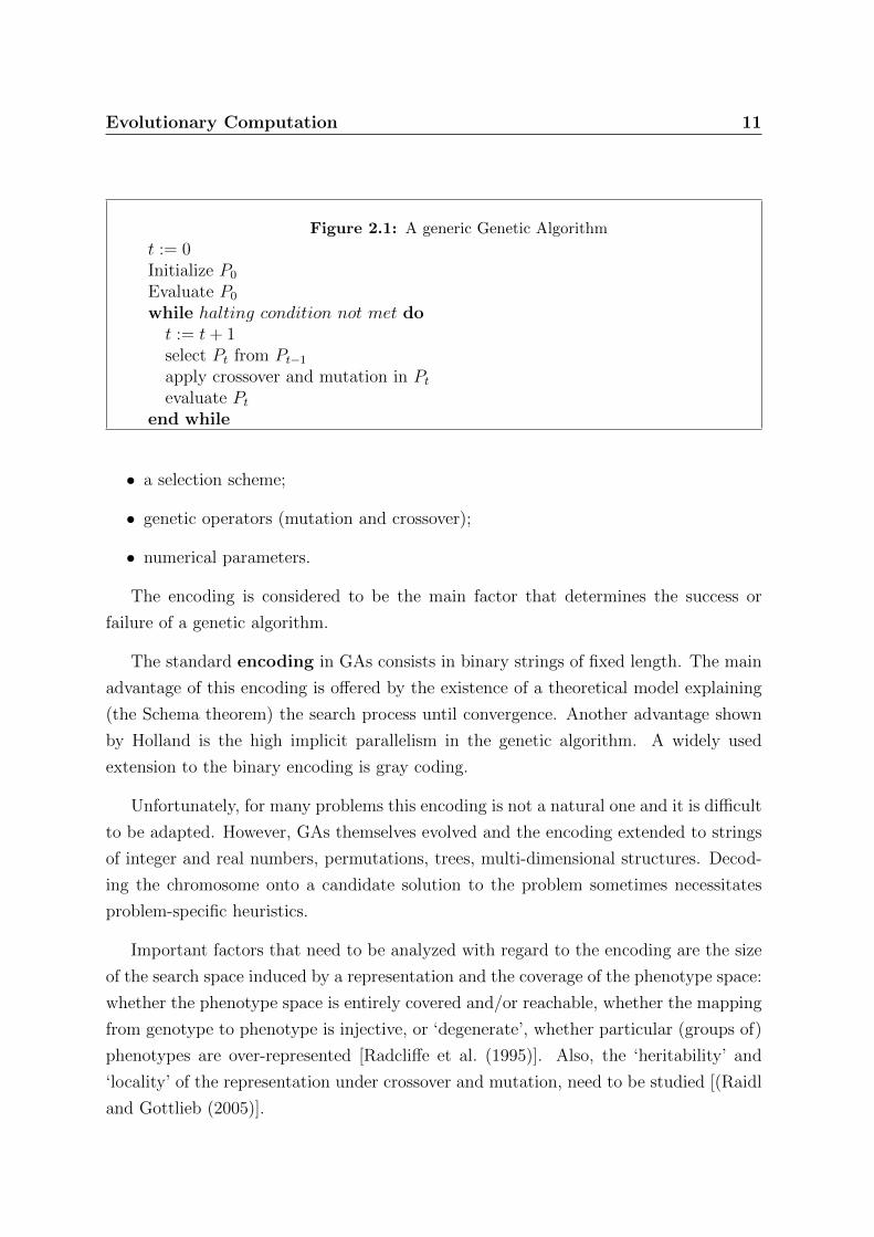
In order to solve a problem with a genetic algorithm, one must define the following
elements:
• an encoding for candidate solutions (the genotype);
• an initialization procedure to generate the initial population of candidate solutions;
• a fitness function which defines the environment and measures the quality of the
candidate solutions;
Evolutionary Computation 11
Figure 2.1: A generic Genetic Algorithm
t := 0Initialize P0
Evaluate P0
while halting condition not met dot := t+ 1select Pt from Pt−1
apply crossover and mutation in Ptevaluate Pt
end while
• a selection scheme;
• genetic operators (mutation and crossover);
• numerical parameters.
The encoding is considered to be the main factor that determines the success or
failure of a genetic algorithm.
The standard encoding in GAs consists in binary strings of fixed length. The main
advantage of this encoding is offered by the existence of a theoretical model explaining
(the Schema theorem) the search process until convergence. Another advantage shown
by Holland is the high implicit parallelism in the genetic algorithm. A widely used
extension to the binary encoding is gray coding.
Unfortunately, for many problems this encoding is not a natural one and it is difficult
to be adapted. However, GAs themselves evolved and the encoding extended to strings
of integer and real numbers, permutations, trees, multi-dimensional structures. Decod-
ing the chromosome onto a candidate solution to the problem sometimes necessitates
problem-specific heuristics.
Important factors that need to be analyzed with regard to the encoding are the size
of the search space induced by a representation and the coverage of the phenotype space:
whether the phenotype space is entirely covered and/or reachable, whether the mapping
from genotype to phenotype is injective, or ‘degenerate’, whether particular (groups of)
phenotypes are over-represented [Radcliffe et al. (1995)]. Also, the ‘heritability’ and
‘locality’ of the representation under crossover and mutation, need to be studied [(Raidl
and Gottlieb (2005)].

Evolutionary Computation 12
The initialization of the population is usually performed randomly. There exist
approaches which make use of greedy strategies to construct some initial good solutions
or other specific methods depending on the problem.
The fitness function is constructed based on the mathematical function to be op-
timized. For more complex problems the fitness function may involve very complex
computations and increase the intrinsic polynomial complexity of the GA.
Several probabilistic procedures based on the fitness distribution in population can be
used to select the individuals to survive in the next generations and produce offsprings.
All these procedures encourage to some degree the survival of the fittest individuals,
allowing at the same time that the worst adapted individual survive and contribute with
local information (short-length substrings) to the structure of the optimal solution. The
most essential feature which differentiates them is the selection pressure: the degree to
which the better individuals are favored; the higher the selection pressure, the more the
better individuals are favored. The selection pressure has a great impact on the diversity
in population and consequently on the convergence of GAs. If the selection pressure is
too high, the algorithm will suffer from insufficient exploration of the search space and
premature convergence occurs, resulting in sub-optimal solutions. On the contrary, if the
selection pressure is too low the algorithm will unnecessarily take longer time to reach
the optimal solution. Various selection schemes were proposed and studied from this
perspective. They can be grouped into two classes: proportionate-based selection and
ordinal-based selection. Proportionate-based selection takes into account the absolute
values of the fitness. The most known procedures in this class are: roulette wheel (John
Holland, 1975) and stochastic universal sampling (James Baker, 1989). Ordinal based
selection takes into account only the relative order of individuals according to their
fitness values. The most used procedures of this kind are the linear ranking selection
(Baker, 1985) and the tournament selection (Goldberg, 1989).
New individuals are created in population with the aid of two genetic operators:
crossover and mutation.
The classical crossover operator aims at exchanging genetic material between two
chromosomes in two steps: a locus is chosen randomly to play the role of a cut point
and splits each of the two chromosomes in two segments; then two new chromosomes
are generated by merging the first segment from the first chromosome with the second
segment from the second chromosome and vice-versa. This operator is called in literature
one-point crossover and is presented in 2.2. Generalizations exist to two, three or more

Evolutionary Computation 13
cut-points. Uniform crossover builds sequentially the offspring by copying at each locus
the allele randomly chosen from one of the two parents.
Various constraints imposed by real-world problems led to various encodings for can-
didate solutions; these problem-specific encodings subsequently necessitate the redefini-
tion of crossover. Thus, algebraic operators are implied for the case of numerical opti-
mization with real encoding; an impressive number of papers focused on permutation-
based encodings proposing various operators and performing comparative studies. It
is now a common procedure to wrap a problem-specific heuristic within the crossover
operator (i.e. [Ionita et al. (2006b)] propose new operators for constraint satisfaction;
chapter 4 of this thesis presents new operators in the context of clustering). Crossover in
GAs stands at the moment for any procedure which combines the information encoded
within two or several chromosomes to create new and hopefully better individuals.
Mutation is a unary operator designed to introduce variability in population. In
the case of binary GA the mutation operator modifies each gene (from 0 to 1 or from 1
to 0) with a given probability. As in the case of crossover, mutation takes various forms
depending on the problem and the encoding used.
When designing a GA, decisions have to be made with regard to several parameters:
population size, crossover and mutation rate, a halting criterion. Except some general
considerations (i.e. high mutation rate in first iterations, decreasing during the run,
combined with a complementary evolution for crossover), finding the optimum parameter
values comes more to empiricism than to abstract studies.
Variations were brought to the classical GA not only at the encoding and operators
level. In order to face the challenges imposed by real-world problems, modifications are
also recorded in the general scheme of the algorithm.
GAs are generally preferred to trajectory-based meta-heuristics (i.e. Hill-Climbing,
Simulated Annealing, Tabu Search) in multi-modal environments, mostly due to
their increased exploration capabilities. However, a classical GA still can be trapped
in a local optimum due to premature attraction of the entire population into its basin
Figure 2.2: One point crossover

Evolutionary Computation 14
of attraction. Therefore, the main concern of GAs for multi-modal optimization is to
maintain diversity for a longer time in order to detect multiple (local) optima. To
discover the global optima, the GA must be able to intensify the search in several
promising regions and eventually encourage simultaneous convergence towards several
local optima. This strategy is called niching : the algorithm forces the population to
preserve subpopulations, each subpopulation corresponding to a niche in the search
space; different niches represent different (local) optimal regions.
Several strategies exist in literature to introduce niching capabilities into evolutionary
algorithms. [Deb and Goldberg (1989)] propose fitness sharing : the fitness of each
individual is modified by taking into account the number and fitness of its closely ranged
individuals. This strategy determine the number of individuals in the attraction basin
of an optimum to be dependent on the height of that peak.
Another widely used strategy is to arrange the candidate solutions into groups of
individuals that can only interact between themselves. The island model evolves inde-
pendently several populations of candidate solutions; after a number of generations indi-
viduals in neighboring populations migrates between the islands [Whitley et al. (1998)].
There are techniques which divide the population, based on the distances between in-
dividuals (the so-called radii-based multi-modal search GAs). Genetic Chromodynamics
[Dumitrescu (2000)] introduces a set of restrictions with regard to the way selection is
applied or the way recombination takes place. A merging operator is introduced which
merges very similar individuals after perturbation takes place.
De Jong introduced a new scheme of inserting the descendants into the population,
called the crowding method [De Jong (1975)]. To preserve diversity, the offspring replace
only similar individuals in the population. The current thesis makes use of the crowding
scheme to perform a multi-modal search in the context of feature selection; the algorithm
employed [Vemuri and Cedeno (1995)] implements the crowding scheme both at selection
and at replacement and is presented in Chapter 6.
A field of intensive research within the evolutionary computation community, is
multi-objective optimization. Most real-world problems necessitate the optimiza-
tion of several, often conflicting objectives. Population-based optimization methods
offer an elegant and very efficient approach to this kind of problems: with small modi-
fications of the basic algorithmic scheme, they are able to offer an approximation of the
Pareto optimal solution set. While moving from one Pareto solution to another, there
is always a certain amount of sacrifice in one objective(s) to achieve a certain amount

Evolutionary Computation 15
of gain in the other(s). Pareto optimal solution sets are often preferred to single solu-
tions in practice, because the trade-off between objectives can be analyzed and optimal
decisions can be made on the specific problem instance.
[Zitzler et al. (2000)] formulate three goals to be achieved by multi-objective search
algorithms:
• the Pareto solution set should be as close as possible to the true Pareto front,
• the Pareto solution set should be uniformly distributed and diverse over of the
Pareto front in order to provide the decision-maker a true picture of trade-offs,
• the set of solutions should capture the whole spectrum of the Pareto front. This
requires investigating solutions at the extreme ends of the objective function space.
GAs have been the most popular heuristic approach to multi-objective design and
optimization problems mostly because of their ability to simultaneously search different
regions of a solution space and find a diverse set of solutions. The crossover operator may
exploit structures of good solutions with respect to different objectives to create new
nondominated solutions in unexplored parts of the Pareto front. In addition, most multi-
objective GAs do not require the user to prioritize, scale, or weigh objectives. There
are many variations of multi-objective GAs in the literature and several comparative
studies. As in multi-modal environments, the main concern in multi-objective GAs
optimization is to maintain diversity throughout the search in order to cover the whole
Pareto front. [Konak et al. (2006)] provide a survey on the most known multi-objective
GAs, describing common techniques used in multi-objective GA to attain the three
above-mentioned goals.
A multi-objective GA known in literature as PESA II [Corne et al. (2001)] is described
in detail in section 4.4 where it is used to solve a graph-clustering problem.
2.3 Swarm Intelligence
Swarm Intelligence (SI) is a computational paradigm inspired from the collective be-
havior in auto-organized decentralized systems. It stipulates that problem solving can
emerge at the level of a collection of agents which are not aware of the problem itself,
but collective interactions lead to the solution. Swarm Intelligence systems are typ-
ically made up of a population of simple autonomous agents interacting locally with

Evolutionary Computation 16
one another and with their environment. Although there is no centralized control, the
local interactions between agents lead to the emergence of global behavior. Examples
of systems like this can be found in nature, including ant colonies, bird flocking, animal
herding, bacteria molding and fish schooling.
The most successful SI techniques are Ant Colony Optimization (ACO) and Particle
Swarm Optimization (PSO). In ACO [(Dorigo and Stutzle (2004))] artificial ants build
solutions walking in the graph of the problem and (simulating real ants) leaving artificial
pheromone so that other ants will be able to build better solutions. ACO was successfully
applied to an impressive number of optimization problems. PSO is an optimization
method initially designed for continuous optimization; however, it was further adapted
to solve various combinatorial problems. PSO is presented in more detail in the next
section.
2.3.1 Particle Swarm Optimization
The PSO model was introduced in 1995 by J. Kennedy and R.C. Eberhart, being dis-
covered through simulation of a simplified social model such as fish schooling or bird
flocking [Kennedy and Eberhart (1995)]. It was originally conceived as a method for
optimization of continuous nonlinear functions. Latter studies showed that PSO can be
successfully adapted to solve combinatorial problems.
PSO consists of a group (swarm) of particles moving in the search space. The trajec-
tory of a particle is determined by local interactions with other particles in the swarm and
by the interaction with the environment. The PSO model thus adheres to the principles
of the Evolutionary Cultural Model proposed by Boyd and Richerson (1985) according
to which individuals of a society have two learning sources: individual learning and
cultural transmission. Individual learning is efficient only in homogenous environments:
the patterns acquired through local interactions with the environment are generally ap-
plicable. For heterogenous environments social learning - the essential feature of cultural
transmission - is necessary.
In the PSO paradigm, the environment corresponds to the search space of the op-
timization problem to be solved. A swarm of particles is placed in this environment.
The location of each particle corresponds therefore to a candidate solution to the prob-
lem. A fitness function is formulated in accordance with the optimization criterion to
measure the quality of each location. The particles move in their environment collecting

Evolutionary Computation 17
information on the quality of the solutions they visit and share this information to the
neighboring particles in the swarm. Each particle is endowed with memory to store the
information gathered by individual interactions with the environment, simulating thus
individual learning. The information acquired from neighboring particles corresponds
to the social learning component.
In the basic version of the PSO algorithm, the formulas used to update the particles
and the procedures are inspired from and conceived for continuous spaces. Therefore,
each particle is represented by a vector x of length n indicating the position in the n-
dimensional search space and has a velocity vector v used to update the current position.
The velocity vector is computed following the rules:
• every particle tends to keep its current direction (an inertia term);
• every particle is attracted to the best position p it has achieved so far (implements
the individual learning component);
• every particle is attracted to the best particle g in the neighborhood (implements
the social learning component).
The velocity vector is computed as a weighted sum of the three terms above. Two
random multipliers r1, r2 are used to gain stochastic exploration capability while w, c1, c2
are weights usually empirically determined. The formulae used to update each of the
individuals in the population at iteration t are:
vti = w · vt−1i + c1 · r1 · (pt−1
i − xt−1i ) + c2 · r2 · (gt−1
i − xt−1i ) (2.1a)
xti = xt−1i + vti (2.1b)
Equation 2.1b generates a new position in the search space (corresponding to a
candidate solution). It can be associated to some extent to the mutation operator
in evolutionary programming. However, in PSO this mutation is guided by the past
experience of both the particle and other members of the swarm. In other words, ”PSO
performs mutation with a conscience” [Shi and Eberhart (1998)]. Considering the best
visited solutions stored in the personal memory of each individual as additional members
of the population, PSO implements a weak form of selection [Angeline (1998)].

Evolutionary Computation 18
The search for the optimal solution in PSO is described by the iterative procedure
in 2.3. The fitness function is denoted by f and is formulated for maximization.
Figure 2.3: Basic PSO
t := 0Initialize xti, i = 1..nInitialize vti , i = 1..nStore personal best pti = xti, i = 1..nFind neighborhood best gti = argmaxy∈Nxti(f(y)), i = 1..nwhile halting condition not met dot := t+ 1Update vti , i = 1..n using equation 2.1aUpdate xti, i = 1..n using equation 2.1bUpdate personal best pti = argmax(f(pt−1
i ), f(xti)) i = 1..nFind neighborhood best gti = argmaxy∈Nxti(f(y)) i = 1..n
end while
Particle pi is chosen in the basic version of the algorithm to be the best position
in the problem space visited by particle i. However, the best position is not always
dependent only on the fitness function. Constraints can be applied in order to adapt
PSO to various problems, without slowing down the convergence of the algorithm. In
constrained non-linear optimization the particles store only feasible solutions and ignore
the infeasible ones [Hu and Eberhart (2002b)]. In multi-objective optimization only the
Pareto-dominant solutions are stored [Coello and Lechunga (2002); Hu and Eberhart
(2002a)]. In dynamic environments particle p is reset to the current position if a change
in the environment is detected [Hu and Eberhart (2001)].
The selection of particle gi is performed in two steps: neighborhood selection followed
by particle selection. The size of the neighborhood has a great impact on the conver-
gence of the algorithm. It is generally accepted that a large neighborhood speeds-up the
convergence while small neighborhoods prevent the algorithm from premature conver-
gence. Various neighborhood topologies were investigated with regard to their impact
on the performance of the algorithm [Kennedy (2002); Kennedy and Mendes (2003)];
however, as expected, there is No Free Lunch: different topologies are appropriate to
different problems.
A major problem investigated in the PSO literature is the premature convergence of
the algorithm in multi-modal optimization. This problem has been addressed in several
papers and solutions include: addition of a queen particle [Clerc (1999)], alternation of

Evolutionary Computation 19
the neighborhood topology [Kennedy (1999)], introduction of sub-populations [Lvbjerg
et al. (2001)], giving the particles a physical extension [Krink et al. (2002)], alterna-
tion between phases of attraction and repulsion [Riget and Vesterstroem (2002)], giving
different temporary search goals to groups of particles [Al-kazemi and Mohan (2002)],
giving particles quantum behavior [Sun et al. (2004)], the use of specific swarm-inspired
operators [Breaban and Luchian (2005)].
Another crucial problem is parameter control. The values and choices for some of
these parameters may have significant impact on the efficiency and reliability of the
PSO. There are several papers that address this problem; in most of them, values for
parameters are established through repeated experiments but there also exist attempts
to adjust them dynamically, using evolutionary computation algorithms. The role played
by the inertia weight was compared to that of the temperature parameter in Simulated
Annealing [Shi and Eberhart (1998)]. A large inertia weight facilitates a global search
while a small inertia weight facilitates a local search. The parameters c1 and c2 are called
generically learning factors; because of their distinct roles, c1 was named the cognitive
parameter (it gives the magnitude of the information gathered by each individual) and c2
the social parameter (it weights the cooperation between particles). Another parameter
used in PSO is the maximum velocity which determines the maximum change each
particle can take during one iteration. This parameter is usually proportional with the
search domain.
Even if PSO was initially conceived for continuous optimization, the algorithm proved
later its applicability to a wide range of combinatorial problems. Versions of binary PSO
were designed [Kennedy and Eberhart (1997)] and the technique was used in integer
programming [Laskari and K.E. Parsopoulos (2002)] and for permutation problems [Hu
et al. (2003)]. Its efficiency was proven in even more complex environments such as
multi-objective optimization [Coello and Lechunga (2002); Hu and Eberhart (2002a)],
constraint optimization [Hu and Eberhart (2002b); Pulido and Coello (2004)], dynamic
environments [Hu and Eberhart (2001)], constraint satisfaction [Breaban et al. (2007);
Ionita et al. (2006a, 2010); Yang et al.]. The use of PSO in cluster analysis is presented
in Chapter 4 of this thesis.
Chapter 3
Clustering
This chapter introduces the problem this thesis is mainly concerned with. The gen-
eral framework of machine learning is unfolded to present the unsupervised context of
clustering. The main difficulties raised by the unsupervised nature of the problem are
highlighted. State-of-the-art algorithms and solution validation criteria are presented.
3.1 Learning from data
It is unnecessary to emphasize here the need for automatic data analysis and information
extraction since it has become ubiquitous nowadays.
By data we commonly denote recorded facts. According to Ackoff (1989), it simply
exists and has no significance beyond its existence (in and of itself). It can exist in
any form, usable or not. It does not have meaning of itself. Information is processed
data: semantic connections give the data a meaning. Extracting implicit, previously
unknown and potentially useful information from data constitutes the object of the
Data Mining field. The algorithmic framework providing automatic support for data
mining is generally called Machine Learning.
Data is usually present in the raw form: records called data items are expressed
as tuples (ordered sequences) of numerical/categorial values; each value in the tuple
indicates the observed value of a feature. The features in a data set are also called
attributes or variables.
20

Clustering 21
Information can be automatically extracted by searching patterns in data. The
process of detecting patterns in data is called learning from data. Depending on the
pattern type, several data mining tasks can be identified.
Association rule mining aims at detecting any association among features. Associa-
tion rules usually involve nonnumeric attributes; the typical application is market basket
analysis, in which the items are articles in shopping carts and the associations among
these purchases are sought.
Classification aims at predicting the value of a nominal feature; the feature in dis-
cussion is called the class variable. Classification is called supervised learning because
the learning scheme is presented with a set of classified examples (the values for the
class variable are given) from which it is expected to learn a way of classifying unseen
examples.
In numeric prediction the outcome to be predicted is not a discrete class but a
numeric quantity.
Clustering is the task of identifying natural groups in data. It is called unsupervised
learning because, even if the outcome is the prediction of a class variable, there aren’t
any training examples provided. Cluster analysis is exploratory or descriptive. There
are no pre-specified models or hypotheses but the aim is to understand the general
characteristics or structure of data. Clustering is the task investigated further in this
thesis.
3.2 The clustering problem
Clustering is a problem intensively studied within the data mining community because
of its wide applicability in diverse fields of sciences, engineering, economy, medicine, etc.
The goal is intuitive, vaguely defined: given a data set, a partition of the data items is
sought such that items belonging to the same cluster are similar while items belonging
to different clusters are dissimilar. The work conducted on clustering converge only at
this general level of description; as for concrete methods, there exist a wide range of
clustering techniques based on different principles and yielding different results. Trying
to unify the initial informal concept of clustering into an axiomatic framework governed
by a unique objective function, Kleinberg (2002) obtains an impossibility result.

Clustering 22
3.2.1 A formal definition
A formal definition of the crisp/hard version of the clustering problem can be stated as
follows:
Given a set S of n data items each of which is described by m numerical attributes:
S = d1, d2, ..., dn where di = fi1, fi2, ..., fim ∈ =1 ×=2 × ...×=m ⊂ <m ∀i = 1..n,
find
C∗ = argmaxC∈ΩF (C)
where
• Ω is the set of all possible hard partitions C of the data set S, where each C is a
hard partition if C = C1, C2, ..., Ck,⋃ki=1 Ci = S and Ci
⋂Cj = ∅ ∀i, j = 1..k,
i 6= j, k ∈ 1, 2, ..., card(C).
• F is a function which measures the quality of each partition C ∈ Ω with respect to
the requirement implicitly described above by the word natural : similar data items
should belong to the same cluster and dissimilar items should reside in distinct
clusters.
Beside crisp clustering, that requires that each object is assigned to exactly one
cluster, clustering is also investigated in more relaxed forms. Rough clustering, inspired
from rough sets theory (Komorowski et al. (1998); Pawlak (1995)), allows for objects
to belong to more than one cluster. In fuzzy clustering (Dumitrescu et al. (2000)) each
object is associated to each cluster with a probability that indicates the strength of the
association between that data item and a particular cluster. Based on the probabilities
computed with a fuzzy clustering procedure, one can obtain a crisp or rough partition.
The current thesis is concerned with the crisp version of clustering.
3.2.2 Learning contexts
As shown in section 3.1, clustering is an exploratory analysis technique performing un-
supervised learning. However, some information can be provided by the user to the
clustering algorithm, introducing some degree of supervision.
If the number of clusters p is known in advance, the problem is called supervised
clustering.

Clustering 23
When a set of constraints is provided in the form of pairs of objects which must
belong to the same cluster or which must reside in different clusters, the problem is
called semi-supervised clustering. The problem has lately received a lot of attention
because in practice labeled data is usually available in a small proportion along with
unlabeled data.
If no information is available with regard to the number of clusters nor with regard
to specific assignments of objects, the problem is called unsupervised clustering.
3.2.3 Challenges
The definition of clustering leaves space to a wide choice of objective functions and
similarity functions, depending strongly on the domain under investigation. The choice
is rarely straightforward. Thus, several challenges can be identified in the clustering
analysis.
An objective function must be formulated to quantify the degree of ”inter-
estingness” or ”naturalness” in groupings. The literature records a lot of comparative
studies regarding the impact of various objective functions on the solution, especially in
the case of unsupervised clustering.
Although in clustering the data items are grouped based on similarity, the notion
of similarity is seldom given in the problem statement. A distance metric is
usually chosen to measure pairwise similarity, prior to applying a clustering procedure.
The metric employed has a great impact on the result of the clustering algorithm since
under different metrics the similarity space changes. If extra-information is available
in the form of pairwise constraints of data items that must reside in the same cluster
(the case of semi-supervised clustering and supervised classification), then an optimal
distance metric can be learned. Unsupervised metric learning is usually performed in a
pre-processing step, using methods that reduce data dimensionality through statistical
analysis. A more in-depth discussion on the importance of metrics in clustering is
conducted in chapter 5.
The definition in section 3.2.1 formulates clustering as an optimization problem. It
is a hard optimization problem due to the huge search space. Even if the number
of clusters is fixed (the case of supervised clustering), the number of possible partitions
increases exponentially with the number of objects; the size of the search space in this
case is given by the Stirling number of the second kind. When the number of clusters is

Clustering 24
not known (the case of unsupervised clustering) the number of ways to partition a set of
n objects into non-empty subsets is given by the nth Bell number. For example, there
are 2 · 1015 ways to partition a set of 25 objects into 5 groups, and more than 4 · 1018
ways to partition them when the number of clusters is not fixed.
3.3 Algorithms
To present efficiently and in a condensed manner the existing (already wide and still
expanding) algorithmic framework for clustering, one would face the challenges of the
clustering analysis itself. There are several excellent surveys which offer a systematic
view of the field: Berkhin (2002); Duda et al. (2001); Jain et al. (1999); Xu and Wun-
sch (2005). The aim of this section is not an exhaustive enumeration of the clustering
algorithms, but a broad outline. The main classes of algorithms are succinctly intro-
duced and more attention is given to the algorithms invoked further across the thesis in
experimental studies.
3.3.1 Hierarchical techniques
Hierarchical techniques build the clusters gradually and make use of a connectivity
matrix expressing the similarity between data items. Two approaches to hierarchical
clustering exist: the agglomerative approach starts with a set of singleton clusters con-
taining only one element and iteratively merge pairs of clusters; the divisive approach
starts with a single cluster containing all objects and iteratively splits one cluster. The
result of a hierarchical clustering algorithm is a tree of clusters called dendrogram.
Merging and splitting clusters necessitate the use of a similarity function defined over
the space of clusters. Several such functions, called linkage metrics were proposed.
Usually the distance between two clusters is computed based on the set of distances
between all pairs of points, with one point in one cluster and another point in the second
cluster. Different operations on this set generate different metrics: the minimum gen-
erates the so-called single linkage metric [Sibson (1973)], the maximum corresponds to
complete linkage [Defays (1977)] and the average to average linkage [Voorhees (1986)].
Single-link and complete-link clustering reduce the assessment of cluster quality to a
single similarity between a pair of objects: the two most similar objects in single-link

Clustering 25
clustering and the two most dissimilar objects in complete-link clustering. A measure-
ment based on one pair cannot fully reflect the distribution of elements in a cluster. It
is therefore not surprising that both algorithms often produce undesirable clusters.
Agglomerative hierarchical clustering can be formulated to optimize explicitly an
objective function; i.e. Ward (1963) designed a hierarchical agglomerative procedure to
minimize in a greedy manner the intra-cluster variance (the sum of squared distances of
all points in the two classes to their mean).
As it is generally the case in clustering, the type of the linkage metric significantly
affects the result because they impose different concepts of closeness. Comparative
studies show that their performance is highly dependent on the data under analysis.
However, average linkage and Ward’s method generally obtain compact clusters with
small diameters while under single linkage the partition can degenerate into chain-like
clusters with less similar objects at the ends.
Since a hierarchy is a natural method of organizing data in various domains, hierar-
chical clustering algorithms are the most used methods in practice. However, the space
and time complexity are unfavorable (O(n2)). Also, an incorrectly placed object in first
iterations can not be reallocated. These methods are not incremental: if new data is
available the algorithm must be restarted to incorporate it.
More sophisticated hierarchical methods exist. Sampling techniques are integrated to
achieve scalability and representatives are used to replace strongly connected data items
in CURE [Guha (2001)], graph partitioning is first performed on the pruned similarity
graph, followed by an agglomerative procedure in CHAMELEON [Karypis et al. (1999)].
3.3.2 Relocation algorithms
Relocation algorithms do not build the clusters gradually, but given a partition (i.e.
randomly generated) they relocate data items among existing clusters in order to improve
them. Usually these methods require an apriori-fixed number of clusters.
The most used methods in this category make use of class representatives/centroids.
These are iterative procedures, which alternate two phases: the data assignment, and
the update of the centroids.
The most popular centroid-based method is K-Means [Forgy (1965)]. As the name
suggests, each cluster is represented by the mean of the points assigned to it. The

Clustering 26
algorithm usually starts with k randomly generated points/centroids in the feature space.
In the batch version, each iteration consists in allocating all data items to the nearest
centroid; then, the centroid of each cluster is updated. In the online/sequential version,
a centroid is updated each time a data item is relocated. Bottou and Bengio (1995) show
that k-Means is a gradient-descent algorithm that minimizes the quantization error using
Newton’s algorithm. They also provide empirical studies on the convergence of k-Means
showing that the online version converges significantly faster than batch k-Means in the
first training epochs but is surpassed in further iterations. These results suggest that
it is better to run the online algorithm during one epoch and then switch to the batch
algorithm. Dhillon et al. (2002) noticed that the batch algorithm tends to get stuck when
applied to document clustering using cosine similarity, while the online algorithm works
better. The batch version has the advantage of allowing straightforward parallelization
[Dhillon and Modha (1999)].
The wide applicability of k-Means is mainly due to its simplicity and its time-
efficiency. For a fixed number of iterations i, n data items described by m attributes and
k clusters the overall complexity is Ø(iknm). However, several important drawbacks can
also be highlighted:
• k-Means is a greedy optimizer delivering local optima and not the global one;
• the result is strongly dependant on the initialization;
• it is sensitive to outliers;
• it is applicable only to numerical data.
Several extensions of k-Means were proposed in literature. Fuzzy c-Means, was pro-
posed by Dunn (1973) and later improved by Bezdek (1981), to allow soft assignments.
Pelleg and Moore (2000) extended k-Means to automatically find the number of clusters
by optimizing a criterion such as Akaike Information Criterion or Bayesian Information
Criterion.
K-Means under the Euclidean metric is known to deliver convex-shaped clusters.
Kernel K-means [Scholkopf et al. (1998)] was proposed to detect arbitrary shaped clus-
ters, with an appropriate choice of the kernel similarity function.
An alternative to the standard k-Means is k-Medians (Kaufman and Rousseeuw
(2005)), which uses as centroid the median of the data instead of the mean.

Clustering 27
Several approaches based on meta-heuristics fall into the relocation class of algo-
rithms for clustering. Most of them search for the class representatives that minimize
the intra-cluster variance (i.e. Simulated Annealing was used by Selim and Alsultan
(1991) and Klein and Dubes (1989), a comparative study between Simulated Annealing,
Tabu Search and a Genetic Algorithm is presented in [Al-Sultana and Khan (1996)]).
Approaches based on EC techniques are presented in more detail in chapter 4.1.
Mixes of hierarchical and relocation algorithms exist. Steinbach et al. (2000) proposed
a hierarchical divisive version of K-means, called bisecting K-means, that recursively
partitions the data into two clusters at each step.
3.3.3 Probabilistic methods
Probabilistic methods were developed based on the idea that the data set corresponds to
a sample independently drawn from a mixture of several populations. The Expectation-
Maximization algorithm iteratively refines an initial cluster model to better fit the data
and terminates at a solution which is locally optimal or a saddle point of the underlying
clustering criterion [Dempster et al. (1977)]. The objective function is the log-likelihood
of the data, given the model measuring how well the probabilistic model fits the data.
An important property of probabilistic clustering is that its applicability is not restricted
to numerical data but can be applied to heterogeneous data as well.
K-Means can be considered a variant of the generalized expectation-maximization
algorithm: the assignment step is referred to as expectation and the update of the
center of the cluster as maximization.
3.3.4 Density-based methods
Density-based clustering methods consider clusters as high density regions in the fea-
ture space separated by low density regions. This interpretation has the advantage of
detecting clusters of arbitrary shapes. Two main concepts are introduced in this con-
text density and connectivity. Both take into account the local distribution in data and
necessitate the definition of neighborhood in data and nearest neighbors computations.
DBSCAN [Ester et al. (1996)] is the most popular algorithm of this kind. Its perfor-
mance depends mainly on two parameters. The neighborhood size is defined in terms
of distance ε. A core point is defined to be a point having a minimum number minPts
Clustering 28
of points in the ε-neighborhood. A point y is said to be directly density-reachable from
a core point if it is in its ε neighborhood. A point y is density reachable from a point
x if there is a chain of points p1, p2, ..., pn, p1 = x, pn = y, such that pi+1 is directly
density-reachable from pi. Two points x and y satisfy the density-connectivity property
if there is a point q such that both x and y are density-reachable from q. The algo-
rithm assigns all points satisfying the density-connectivity relation to one cluster. One
important drawback of DBSCAN is that there is no straightforward way to fit the two
parameters to data. OPTICS [Ankerst et al. (1999)] was proposed to overcome part of
this drawback by covering a range of increasing values for the neighborhood size.
3.3.5 Grid-based methods
The grid-based clustering algorithms work indirectly with data: they segment the fea-
ture space and then they aggregate dense neighbor segments. A segment is a multi-
rectangular region in the feature space, result of the Cartesian product of individual
feature subranges. Data partitioning is practically achieved through space partitioning.
There are grid-based methods that prune the attribute space in an Apriori man-
ner, performing subspace clustering. Subspace clustering is motivated in case of high-
dimensional data, when irrelevant features can mask the grouping tendency. It is an
extension of traditional clustering that seeks to find clusters in different subspaces within
a data set. The most popular grid-based algorithms of this type are CLIQUE [Agrawal
et al. (2005)] and ENCLUS [Ada et al. (1999)].
3.3.6 Ensemble clustering
Various clustering techniques generate various partitions of data. To reach a consensus
over the various partitions that can be extracted and to hopefully obtain a better one,
ensemble techniques were designed.
Combining multiple clustering algorithms is a more challenging problem than com-
bining multiple classifiers.
Recent literature on clustering records several ensemble techniques which combine
individual clusterings [Fred and Jain (2005); Strehl and Ghosh (2002)] and various em-
pirical studies concerning the performance of these techniques [Hu et al. (2006); Zhou
and Tang (2006)]. Much work was conducted on ensemble construction. The bagging

Clustering 29
technique was borrowed from supervised classification [Dudoit (2003)] and the boosting
method was adapted to the unsupervised case [Topchy et al. (2004)]. Random feature
subspaces were used to create weak but diverse clusterings [Topchy et al. (2003)], ran-
dom projections is adopted to construct clusters in low dimensional spaces[Urruty et al.
(2007)], different clustering algorithms were applied [Strehl and Ghosh (2002)], or a clus-
tering method is applied repeatedly with different parameters/initializations [Jain and
Fred (2002)].
There are studies tracking the properties that make all the difference to the quality
of the final clustering result [Hadjitodorov et al. (2006); Hu et al. (2006)]. They mainly
address the following questions: how accurate and how diverse should input partitions
be?; how many components are needed to ensure a successful combination? A unani-
mously accepted result is that diversity and accuracy are mandatory features for good
ensembles. Hu et al. (2006) suggest that a limited and controlled diversity is preferred
for ensemble construction; the intuition behind it is that the component clusterings
differ only in the instances whose assignments are incorrect and these errors could be
complemented or canceled during the combination. If various clustering algorithms pro-
duce largely different results due to different clustering criteria, combining the clustering
results directly with integration rules, such as sum, product, median and majority vote
can not generate a good meaningful result.
Section 6.4 of the thesis presents in detail an ensemble clustering procedure.
3.4 Optimization criteria
As formulated in section 3.2.1, clustering is an optimization problem that lacks a general-
accepted objective. Various algorithms optimize (explicitly or not) various objectives.
This section outlines the objectives optimized implicitly by the traditional clustering
approaches and surveys clustering criteria proposed to be optimized explicitly by various
(meta)heuristics. A distinction is made with respect to the available information on the
number of clusters.
The objective functions presented here are called in literature internal clustering
criteria, as they assess the fit between the structure and the data using only the data
themselves.

Clustering 30
3.4.1 Known number of clusters
Popular clustering techniques like hierarchical approaches and k-Means necessitate the
number of clusters to be known. They are greedy methods optimizing implicitly various
objectives.
Centroids-based methods work towards minimizing the deviation of data items from
the cluster representatives. In k-Means the centroid corresponds to the mean, which lead
to the implicit minimization of the intra-cluster variance. Just as the mean minimizes
the standard deviation, the median minimizes average absolute deviation; thus, k-
Medians minimizes implicitly and in a greedy manner the average absolute deviation.
The two methods can be regarded as both optimizing the same objective - the error over
all clusters - but k-Means optimize it with respect to the Euclidean metric, while k-
Medians optimize it with respect to the Manhattan metric.
The intra-cluster variance is the simplest and the most used criterion for clustering,
being also explicitly optimized with general search algorithms. It is also known in
literature as the sum-of-squared-error criterion (Duda et al. (2001)). It is defined in
equation
Cse =k∑j=1
∑d∈Cj
δ2(cj, d) (3.1)
where cj = 1|Cj |∑
d∈Cj d is the mean of cluster Cj, δ is the Euclidean distance and by
|Cj| we denote the cardinality of cluster Cj.
This criterion is appropriate for data containing clusters of equal volumes; it is also
sensitive to outliers. These situations degenerate into drawbacks for k-Means, and are
illustrated in section 4.2.4 of this thesis.
By simple computations the mean vectors can be eliminated from equation 3.1 and
the following equivalent criterion is obtained:
Cse =1
2
k∑j=1
1
|Cj|∑d∈Cj
∑d′∈Cj
δ2(d, d′) (3.2)

Clustering 31
Using statistics terminology, intra-cluster variance is unexplained/residual variance.
Summed up to the explained variance it gives the total variance in data. Then, a criterion
equivalent to 3.1 but necessitating maximization is the following:
Cse =k∑j=1
|Cj|δ2(cj, c) (3.3)
where c = 1|S|∑
d∈S d is the mean of the entire data set.
In the case of hierarchical algorithms and density-based methods, to derive a global
optimization criterion is not such a straightforward task, because these methods base
their decisions on the local distribution in data. It was established (Fraley and Raftery
(2002); Kamvar et al. (2002)) that classical agglomerative algorithms have quite complex
underlying probability models. The Single-Link algorithm is represented by a mixture of
branching random walks, while the Average-Link algorithm is equivalent to finding the
maximum likelihood estimate of the parameters of a stochastic process with Laplacian
conditional probability densities.
The use of the Complete-Link or of the minimum-variance criterion (Ward’s method)
relates more to squared error methods. The use of the single-link criterion can be related
to density-based methods. The average-link algorithm optimizes greedily a criterion
widely known in graph partitioning as minimum cut:
CMC =k−1∑i=1
k∑j=i+1
∑d∈Ci
∑d′∈Cj
δ(d, d′) (3.4)
The above clustering criteria are sensitive to axes scaling: different partitions may
be obtained if the data is subject to linear transformations.
An invariant criterion, frequently used in literature, can be formulated based on the
so-called scatter matrices of a partition. The scatter matrix of a cluster Ci is the matrix
Si ∈ <m×m, Si =∑
d∈Ci(d− ci)(d− ci)t. The within-cluster scatter matrix is the sum:
SW =k∑i=1
Si (3.5)

Clustering 32
The trace of the within-cluster matrix is exactly criterion 3.1.
The between-cluster scatter matrix SB ∈ <m×m is built based on the means of the
clusters (ci) and the mean of the entire data set (c):
SB =k∑i=1
(ci − c)(ci − c)t (3.6)
The trace of the between-cluster scatter matrix is identical to criterion 3.3.
An invariant clustering criterion can be formulated based on the property that the
eigenvalues of S−1W SB are invariant under linear transformations of the data; then, func-
tions of these eigenvalues can be used. Because the trace of a matrix is the sum of its
eigenvalues, a widely used invariant clustering criterion necessitating maximization is:
CWB = tr[S−1W SB]. (3.7)
As highlighted in (Duda et al. (2001)), if different apparent clusters can be obtained
by scaling the axes or by applying any other linear transformation, then all of these
groupings will be exposed by invariant procedures. For this reason, invariant clustering
criteria are likely to possess multiple local optimum, being more difficult to optimize.
3.4.2 Unknown number of clusters
The clustering criteria presented above (section 3.4.1) can be used only in the supervised
context of clustering, when the number of clusters is known. If they are used to order
partitions with various numbers of clusters, the extreme case - the partition consisting
of n singleton clusters - will be preferred. To identify the optimal number of clusters in
this case, the elbow method can be used: the problem is solved repeatedly for different
values of k and the criterion is computed in all cases; a large gap in the criterion values
suggests the optimal number of clusters. This method is also employed in the case of
hierarchical algorithms with respect to the linkage-metric.
A real challenge in clustering is the design of objective functions able to rank highest
the partition with the optimal number of clusters. Such clustering criteria will be referred
further in this thesis as unsupervised criteria. Several studies exist in literature with this
aim.

Clustering 33
The most popular indices of this type are given below.
Silhouette Width (Rousseeuw (1987)) is shown in several studies to be superior over
other unsupervised clustering criteria (Handl and Knowles (2006a)). SW for a partition
is computed as the average silhouette over all data items in the data set. The Silhouette
for a data item i is computed as follows:
S(i) =bi − ai
max(bi, ai)(3.8)
where
ai = avgd∈Ciδ(di, d) where di ∈ Ci, denotes the average distance between i and all
data items in the same cluster;
bi = minC 6=Ciavgd∈Cδ(di, d) where di ∈ Ci, denotes the average distance between i
and all data items in the closest other cluster (defined as the one yielding the minimal
bi).
SW takes on values in the range [-1,1] and is to be maximized in search of the optimal
clustering.
Another widely used clustering criterion is Davies-Bouldin Index (DB) (Davies
and Bouldin (1979)) which makes use of cluster representatives to compute the within-
cluster compactness and between-cluster separation in a partitioning:
WDB(j) = 1|Cj | ·
∑d∈Cj δ(cj, d) is the intra-cluster compactness for cluster Cj;
BDB(j, l) = δ(cj, cl) is the separation between clusters Cj and Cl.
The DB Index is defined as:
IDB =1
k·
k∑j=1
maxj,l 6=j
(WDB(j) +WDB(l)
BDB(j, l)
)(3.9)
and is to be minimized in order to seek for the optimum clustering.
The Dunn Index (Dunn (1974)) measures the ratio between the smallest inter-cluster
distance and the largest intra-cluster distance in a partition:

Clustering 34
D = mini=1,k
minj=1,k
dist(Ci, Cj)
maxl=1,k diam(Cl)(3.10)
where diam(Cl) is the maximum intra-cluster distance within cluster Cl and
dist(Ci, Cj) is the minimal distance between pairs of data items placed in the distinct
clusters Ci and Cj. The Dunn index is to be maximized in order to seek for the optimum
clustering.
Section 7.4.3 of this thesis presents some comparative studies on the performance of
the above criteria.
Bezdek and Pal (1998) evaluate several indices for crisp clustering. They identify two
deficiencies of Dunn’s index which make it overly sensitive to noisy clusters and propose
several generalizations of it that are not as brittle to outliers in the clusters.
Raskutti and Leckie (1999) propose and study several clustering criteria. They com-
pare the number of clusters chosen by the proposed criteria with the number of clusters
chosen by a group of human subjects. The empirical study demonstrates that there are
usually several significant sets of clusters that can be extracted, rather than a single set
of clusters that is the clear winner.
3.5 Solution evaluation
The quality of a partition can be quantified using external clustering criteria that mea-
sure performance by matching a clustering structure to a priori information. This section
lists the external clustering criteria used in experimental sections across this thesis to
measure the match between partitions returned by the investigated algorithms and the
true partition of the data.
The match between two partitions C and U can be expressed with the aid of the
contingency matrix (also called confusion matrix) M ∈ <kC×kU (kC and kU give the
number of clusters in C, respectively U) where Mij = |Ci⋂Uj| gives the number of data
items placed in cluster Ci in C and in cluster Uj in U.
Given two partitions C and U, the Rand Index (RI) records the following information:

Clustering 35
• a - the number of pairs of data items that are placed in the same cluster in C and
in the same cluster in U
• b - the number of pairs of objects in the same cluster in C but not in the same
cluster in U
• c - the number of pairs of objects in the same cluster in U but not in the same
cluster in C
• d - the number of pairs of objects in different clusters in both partitions.
The Rand Index is computed as (a+ d)/(a+ b+ c+ d). The quantities a and d can be
interpreted as agreement, while b and c as disagreement.
It is desirable that the similarity measure takes values close to 0 for two random
partitions and value 1 for identical partitions. To this goal, a normalization by the results
expected from random data is needed. The Adjusted Rand Index Hubert (1985), which
incorporates such normalization, can take on values in a wider range, thus increasing
the sensitivity. In general, the normalization corrects the estimated absolute degree of
quality. The Adjusted Rand Index is given by the formula:
ARI =
∑ij C
2Mij−[∑
iC2Mi−·∑
j C2M−j
]/C2
M
12
[∑iC
2Mi−
+∑
j C2M−j
]−[∑
iC2Mi−·∑
j C2M−j
]/C2
M
(3.11)
where Mij is the number of data items both in cluster i in C and in cluster j in U,
Mi− is the number of data items in cluster i in C (the sum on row i in M) and M−j is
the number of data items in cluster j in U (the sum on column i in M).

Chapter 4
Evolutionary Computation in
clustering
As seen in chapter 2, Evolutionary Computation techniques are general-purpose op-
timization methods that rely on the feedback of the system to discover and exploit
properties specific to the problem instance under analysis. Because of its huge search
space and its unsupervised nature, clustering is a good candidate at optimization for
these methods.
This chapter presents approaches to clustering based on Evolutionary Computation
techniques. Section 4.1 surveys existing work. A hybridization between k-Means and
PSO aiming at improving the performance of the centroid-based method is presented in
section 4.2. Community detection in social networks is investigated in section 4.3 and a
multi-objective graph clustering problem in section 4.4.
4.1 Clustering techniques based on EC
This section surveys existing work in clustering with EC techniques. The field is quite
wide, as numerous attempts to use EC techniques in clustering exist. We provide a
systematic view, triggered by the kind of solution encoding. The encoding inevitable
relates the method to one of the traditional clustering techniques presented in section
3.3 of this thesis; therefore, the current section is organized similarly.
36

Evolutionary Computation in clustering 37
4.1.1 Relocation approaches
Because generally in EC techniques, a population of complete solutions evolves during
an iterative process, most approaches to clustering are relocation methods, that improve
initially generated partitions. Several encodings were proposed to represent partitions.
First attempts to use Evolutionary techniques in clustering date back to 1991 when
Krovi (1991) proposed a genetic algorithm to search for the optimal partition of a data
set into 2 clusters. The straightforward group-encoding representation is used:
solutions are strings of integers, of length equal with the size of the data set, the i’th
integer signifying the cluster number of data item i. Used in conjunction with classical
genetic operators, this encoding suffers from several drawbacks like redundancy and in-
validity and determines a slow convergence of the algorithm. The algorithm maximizes
the ratio of the between sum-of-squares and the within sum-of-squares. The same repre-
sentation is used by Krishna and Narasimha Murty (1999) to search for a partition with
a fixed number of clusters using modified genetic operators. Crossover is replaced with
one k-Means iteration: the centroid (mean) of each cluster is computed and each data
item is reassigned to the nearest centroid; mutation takes into account the distances to
clusters centroids.
Permutations are used in several ways to render a partition. Jones and Beltramo
(1991) encode a solution as a permutation that gives an ordering of the objects and
separators that indicate the cluster boundaries. A greedy permutation representation
uses the objects on the first k positions in the permutation as cluster representatives, the
rest of the objects being assigned to the nearest representative. Crossover and mutation
operators dedicated to permutation encodings are used.
Bezdek et al. (1994) encode a partition as a boolean k × n matrix. The criterion
to be minimized is the sum-of-squared-errors. They experiment with several distance
metrics in order to detect clusters of various shapes. The crossover operator swaps
columns between two chromosomes. Mutation simply changes randomly the cluster
assignment of one object.
Luchian et al. (1994) proposed a new encoding which considers cluster represen-
tatives, allowing for simultaneous search of the optimum number of clusters and the
optimum partition. The partition is constructed in a manner similar to k-Means: the
data items are assigned to clusters based on the proximity to the cluster representatives.
Crossover and mutation operators are adapted to work with variable-length chromo-

Evolutionary Computation in clustering 38
somes and real encoding. A lamarckian operator that acts at gene level and modifies
a cluster representative to match the mean of the corresponding cluster is introduced.
This can be interpreted as a hybridization with k-Means since the cluster assignment
procedure and the update of the cluster representative constitute one iteration of this tra-
ditional clustering method. However, experimental results show that this hybridization
can lead to premature convergence due to an increased selection pressure. Unsupervised
clustering criteria able to evaluate and order partitions with various number of clusters
are used. Hall et al. (1999) extend the algorithm to search for fuzzy partitions with
fixed number of clusters. Gray coding is used to encode cluster representatives. This
representation became the most successful in the EA clustering literature [Maulik and
Bandyopadhyay (2000); Pan et al. (2003)]. The criterion optimized in approaches of this
kind is the compactness computed based on the distances between the data items and
the cluster centers.
Mostly because of its design for continuous optimization, many approaches to clus-
tering based on PSO use the centroid-based encoding presented in Luchian et al. (1994)
and search for cluster representatives. The performance of these approaches is compared
to the standard k-Means algorithm (with the real number of clusters) and is reported
to be significantly better - or equal in performance in case k-Means is supplied the best
initial configuration. The improved performance is due to the increased exploration
capabilities, eliminating one important drawback: strong dependency on initialization.
However, other drawbacks may still be present: the result is dependent on the metric
used and clusters with similar shapes and volumes tend to be formed. A survey on
Swarm Intelligence techniques applied to clustering can be found in Abraham et al.
(2007).
Differential evolution was used in the supervised [Abraham et al. (2006)] and unsu-
pervised scenario [Zaharie et al. (2007)] with a centroid-based encoding.
A notable contribution the field of Evolutionary Computation made to clustering
is the use of multi-objective algorithms, which allow for simultaneous optimization of
several criteria. han optimize both intra-cluster variance and connectivity. They use
the locus-based adjacency representation. A value j assigned to the ith gene, is
interpreted as a link between data items i and j: in the resulting clustering solution they
will be in the same cluster. The decoding of this representation requires the identification
of all connected components. All data items belonging to the same connected component
are then assigned to one cluster. The representation is well-suited for the use with
standard crossover operators. Moreover, this encoding allows, in conjunction with an

Evolutionary Computation in clustering 39
objective function based on connectivity, to discover clusters of various shapes. The
method improves substantially over traditional methods like k-Means and hierarchical
versions, methods which optimize a single objective from the two under consideration.
4.1.2 Density-based approaches
In the category of density-based approaches for clustering we integrate multi-modal
evolutionary algorithms that search for cluster centers that lie in dense regions in the
feature space [Dumitrescu and Simon (2003); Nasraoui et al. (2005); Zaharie (2005)].
Gaussian functions are used to measure the fit of cluster centroids.
Nasraoui et al. (2005) suppose that data are distributed according to normal distri-
butions: each cluster will be a hyper-ellipsoid characterized, by a mean and a covariance
matrix. A multi-modal genetic algorithm is used to find local maxima of a density func-
tion. An individual in the population represents a point in the m-dimensional feature
space with the aim of identifying centers of dense regions. The scales and orientation
parameters of clusters are adjusted by estimating them using the current values of the
centers.
Zaharie (2005) analyzes the applicability of a crowding Differential Evolution algo-
rithm in the same context. The author evolves not only the number of clusters, but
also the hyper-ellipsoid scales. Additionally, compared to the method in (Nasraoui et al.
(2005)) that generates one descriptor for each cluster in this approach a set of descrip-
tors can be associated to the same cluster. The proposed approach ensures a reliable
identification of clusters in noisy data providing in the same time multi-center synthetic
descriptions for them.
4.1.3 Grid-based approaches
Sarafis et al. (2002) use a genetic algorithm to search for a partition of the feature space
that implicitly provides a partition of the data set. The algorithm evolves rules which
build a grid in the feature space. Each individual consists of a set of k clustering rules,
each rule corresponding to one cluster. Each rule is constituted from m genes and each
gene corresponds to an interval involving one feature. The authors attempt to allevi-
ate certain drawbacks related to the classical minimization of square-error criterion by
suggesting a flexible fitness function which takes into consideration, cluster asymmetry,

Evolutionary Computation in clustering 40
density, coverage and homogeneity. The method is able to discover clusters of various
shapes, sizes and densities. This comes at a high computational cost due to the form of
the fitness function.
4.1.4 Manifold learning
Inspired by dimensionality reduction techniques, Swarm Intelligence algorithms were
designed to embed the original data set into a lower-dimensional feature space which
preserves the topological relationships among data items. ACO was used to arrange
data items within the cells of a two-dimensional grid, representation well-known from
Self Organizing Maps (Kohonen, 1995); a rigorous study on the performance of this
approach can be found in Handl et al. (2005).
A mapping of the original data set into a two-dimensional Euclidean space is per-
formed using simple PSO rules [Veenhuis and Koeppen (2006)]; although a metric space
is employed, the approach is not aimed at generating an embedding of the original data
which faithfully preserves the original pairwise distances among data items (as in Mul-
tidimensional Scaling approaches); the focus is on identifying clusters through species
separation metaphor. Breaban et al. (2009) use a similar technique to find communities
in social networks; the method is detailed in section 4.3.
4.2 Introducing the Connectivity Principle in
k-Means
Traditional approaches to clustering are single-objective optimizers that take into ac-
count either the global distribution in data (it is the case of relocation methods like
k-Means, probabilistic methods), either local information (i.e. density-based methods,
hierarchical methods) but not both. In essence, clustering can be seen as a multi-
objective optimization problem. Nevertheless, few multi-objective clustering strategies
have been proposed; the existing approaches are based on multi-objective evolutionary
techniques.
This section approaches clustering as a multi-objective problem and proposes a
method which is a hybridization between k-Means and a Swarm Intelligence technique
(PSO-kMeans). The work presented here is an extension of a previous study that uses

Evolutionary Computation in clustering 41
PSO as a preprocessing step to better outline clusters in data [Breaban and Luchian
(2008)]. PSO is used this time to introduce the connectivity principle (specific to density-
based methods) into k-Means (a centroid-based clustering approach). The proposed
method alleviates some drawbacks of the k-Means algorithm; thus, it is able to identify
types of clusters which are otherwise difficult to obtain (elongated shapes, non-similar
volumes). Experimental results show that PSO-kMeans improves the performance of
standard k-Means in all test cases and performs at least similar to state-of-the-art meth-
ods in the worst case. PSO-kMeans is robust to outliers. This comes at a cost: the pre-
processing step for finding ns nearest neighbors for each of the n data items is required,
which increases the initial linear complexity to O(n2) including distance computations
among data items.
4.2.1 Motivation
K-Means is the most popular clustering algorithm due to its simple implementation, low
run-time and space complexity and simple usage since no parameters (except the number
of clusters) are involved. However, all these advantages come at a cost: performing a local
search, its performance is highly dependent on initialization. Moreover, its applicability
is reduced to the case of data sets with spherical clusters of almost-equal volumes.
The first drawback is partially alleviated if a smarter initialization scheme is used.
The initial centroids should be placed far apart, or a hierarchical clustering method may
be used to return an initial partition over a small sample of the data set. The most
comfortable way to deal with this drawback (but at the same the most time-consuming)
is to run k-Means repeatedly with random initializations and choose the one with the
lowest intra-cluster variance.
The second drawback is met to all clustering algorithms based on representatives:
under the Euclidean metric spherical clusters are generated. Even if the centroids-based
clustering methods based on Genetic Algorithms or Swarm Algorithms tackle the first
drawback (dependency to initialization), they cannot generate clusters of various shapes.
In order to deal with clusters of various shapes, a more local concept of clustering
must be introduced: neighboring data items should share the same cluster. We propose
a Swarm algorithm called PSO-kMeans which implements the connectivity principle and
introduce it within k-Means taking thus into account simultaneously the local and the
global distribution in data.

Evolutionary Computation in clustering 42
4.2.2 The Hybridization
The connectivity principle was introduced in different forms in clustering algorithms.
In density-based approaches it works towards putting in the same cluster neighboring
data items that form dense regions. Handl and Knowles (2005) formulate and maximize
explicitly by means of GAs, a connectivity objective defined as the number of neighboring
data items which reside in the same cluster.
We propose another approach for implementing the connectivity principle, much of
it inspired from metric learning. In supervised metric learning, a metric is learned
so that the distance between similar data items is as small as possible under the new
metric. In our unsupervised context, similarity is defined with respect to the Euclidean
distance: neighboring data items in the Euclidean space are considered to be similar.
Consequently, in PSO-kMeans the distance between neighboring data items is shortened
by modifying their representation with the aid of the PSO paradigm.
Generally, in solving optimization problems with PSO, the position vectors x cor-
respond to complete candidate solutions and the particles p and g which dictate the
particles’ motion are chosen with regard to a fitness/objective function from the popu-
lation (see section 2.3.1).
In our approach for clustering, each particle corresponds to a data item in the data
set. The feature space defined by the data set provides the environment for the swarm
of particles. The position vector x of each particle is initialized with the feature vector
of the corresponding data item. The original PSO rules that dictate the motion of each
particle are used to change the representation of each data item. No objective function
is explicitly formulated, but through an appropriate definition of the vectors p and g in
equation 2.1a the connectivity is maximized.
Each particle updates its position to match its nearest neighbors. With this aim, each
particle xi should move iteratively towards each of its neighbors. In order to reduce the
run time, a centroid over the neighbors is computed and the particle moves towards it.
This centroid plays the ”pi” role in formula 2.1a. Its use accounts for local distribution
in data.
To take into account the global distribution in data, ”gi” is defined to be the centroid
closest to particle i in the partition returned by k-Means.
The new clustering algorithm is presented succinctly in pseudocode 4.1.

Evolutionary Computation in clustering 43
Figure 4.1: PSO-kMeans
Require: The set of data items D = x1, x2, ..., xn, the number of clusters k.Ensure: a hard partition C = C1, C2, ..., Ck,
⋃ki=1 Ci = D and
Ci⋂Cj = ∅∀i, j = 1..n.
// preprocessing step:for all data item xi doNNi ← the ns nearest neighbors for xi
end for
// initialization phase:apply k-Means until convergence and store:C ← C1, C2, ..., Ck, the hard k-Means partition;cj ← 1
|Cj |∑
xi∈Cj xi the centroid of cluster j, ∀j = 1..k;
di ← dist(xi, cj), ∀i = 1..n, where cj is the centroid of cluster Cj ∈ C and xi ∈ Cj,dist is the Euclidean distance;σ2 ← 1
n
∑ni=1 d
2i (approximates the variance within clusters)
//the PSO-kMeans iterations:while C has not changed for itr iterations do
//run one PSO iteration:for i← 1 to n dopi ← 1
|NNi|∑
xj∈NNi xjgi ← cj s.t. xi ∈ Cjupdate xi applying formulae 4.1
end for
//run one k-Means iteration:for i← 1 to n do
reassign xi to Cj, where Cj = argmincl,l=1..kdist(xi, cl)end forfor j ← 1 to k docj ← 1
|Cj |∑
xi∈Cj xiend for
end while

Evolutionary Computation in clustering 44
A pre-processing step is required to find the ns nearest neighbors of each particle.
This set of neighbors is computed only once, at the beginning, and is not modified
throughout the run. In this way, subsequent changes of the positions of the data items,
which correspond to changes in the representation of the data items to be clustered,
preserve much of the initial topology.
The batch version of the k-Means algorithm is run until convergence. The centroids
retrieved with k-Means serve further as gi in the first iteration of PSO.
Then, an iterative process begins that alternates a PSO iteration with a k-Means
iteration until a stable partition is reached. The PSO iteration consists of recomputing
pi and applying formulae 4.1 which modify each data item xi in the data set. The
particle pi is updated using the same set of neighboring data items computed in the
pre-processing step; because all particles/data items are subjected to the PSO updating
rules, the configuration of the neighborhood changes implicitly.
The k-Means iteration comes to rebuild the partition and reassigns the modified data
items to the previous found centroids. The centroids gi are updated.
Parameters
The initial velocity is set to 0 for all particles. The random multipliers in formula 2.1a
of the basic PSO are not needed. The weights for the inertia term and for the pi term
are set to 1. Preliminary experiments showed that the inertia term has an important
influence on the speed of convergence: the number of iterations in PSO-kMeans reduces
to almost a half for some data sets in its presence, compared to the case when it is not
used at all.
If a unit weight is given also to the third term in equation 2.1a, the impact of our
hybridization is much reduced: almost all particles will end up in the centroids identified
with k-Means on the original representation of the data set. Generally in k-Means, for a
given cluster the data items situated closer to the centroid are more likely to belong to
the corresponding cluster than the data items situated farther (fuzzy k-Means originates
from this principle). For this reason we apply the third update rule in equation 2.1a (the
move towards the cluster centroid) on only 10% of the data items situated closest to the
centroid. For clusters obeying the normal distribution, 10% data items are supposed
to lie within a distance of 0.125 standard deviations from the centroid. To reduce the
computational cost, we adopt the hypotheses of normal distribution and apply the third
updating rule on the data items satisfying the property above; however, this does not

Evolutionary Computation in clustering 45
restrict the use of our method on other types of distributions. The average within-
cluster variance σ2 is computed in the k-Means iteration when data items are assigned
to clusters. A vector of length n (the number of data items) is used to store at this step
the distances between each data item i and its closest centroid gi. Using the average
over all clusters of the within-cluster variance instead the exact values computed for each
cluster in turn, brings some advantages. Well-initialized cluster centroids will ”consume”
most of this rule compared to wrongly placed centroids. The particles on the boundary of
the clusters are attracted to their neighbors situated closer to the centroids and migrate
together to the center of the cluster, leading to more stable clusters.
Formulae 4.1 are used to update the representation xi of the data item i at iteration
t.
vti = vt−1i + (pi − xt−1
i ) + w(i) · (gi − xt−1i ) (4.1a)
xti = xt−1i + vti (4.1b)
w(i) =
1, dist(xt−1i , gi) < 0.125 · σ
0, otherwise(4.1c)
4.2.3 Experiments
The performance of PSO-kMeans is studied on artificial and real data sets, in the su-
pervised context of clustering (when the number of clusters is known) and also in the
unsupervised context (when the number of clusters is not known).
Datasets
In order to test the technique we propose, some complex data sets made available by
Julia Handl 1 are used:
• a standard cluster model using multivariate normal distributions. Different com-
binations number of attributes / number of clusters are considered, as described
in Table 4.1. In low dimensions (2 features), the clusters generated are frequently
1http://dbkgroup.org/handl/generators/

Evolutionary Computation in clustering 46
Parameter Gaussian datasets Ellipsoidal datasets
#attributes 2, 10 50
#clusters 4, 10, 20 4, 10, 20
Size of each cluster uniformly in [50, 500] for datasets uniformly in [50, 500] for datasets
with 4 and 10clusters, with 4 and 10clusters
and uniformly in [10, 100] and uniformly in [10, 100]
for datasets with 20 clusters for datasets with 20 clusters
Table 4.1: Parameters for the artificial data sets
elongated and of arbitrary orientation but in high dimensions (10 features) they
tend to become spherical. The clusters have various volumes/densities.
• data sets of high dimensionality consisting of ellipsoidal clusters with the major
axis of arbitrary orientation. The parameters are explained in Table 4.1.
For each combination of number of attributes / number of clusters 10 different prob-
lem instances were generated and referred to as the group of problems (#attributes)d-
(#clusters)c.
The real data sets used are Iris, Soybean, and Breast Cancer from UCI Repository2.
Experimental setup
In order to test the performance of PSO-kMeans in the supervised context of clustering,
50 runs of the algorithm are performed for each dataset. Random initialization is used
at each run, each cluster centroid being initialized with a randomly chosen data item
from the dataset.
The performance of PSO-kMeans is compared to the batch version of the standard k-
Means. The Adjusted Rand Index (equation 3.11) is computed for the partition derived
with k-Means in the initialization phase of PSO-kMeans and then for the partition
obtained at the end of PSO-kMeans. Both the number of iterations required for standard
k-Means to reach convergence and the additional number of iterations performed in PSO-
kMeans until convergence are reported.
2http://archive.ics.uci.edu/ml/

Evolutionary Computation in clustering 47
If we are willing to substitute the standard k-Means with PSO-kMeans, one important
concern arises with regard to the optimum number of clusters. Because PSO-kMeans
modifies the representation of data items and consequently the distances among them,
there exists the risk of breaking one initial cluster into several smaller dense clusters, case
which misleads the unsupervised clustering analysis. Therefore, experimental analysis
is required for the unsupervised scenario of clustering.
In the unsupervised context, when the number of clusters is not known in advance,
the optimal partition can be obtained as follows: k-Means is run iteratively with k in a
wide range of values and the resulted partitions having different numbers of clusters are
evaluated using an unsupervised clustering criterion (see section 3.4.2 for unsupervised
clustering criteria). The winning partition and consequently the optimum number of
clusters is considered to be the one with the best score under one of these criteria.We
adopt this scenario to study PSO-kMeans in the unsupervised context: an unsupervised
clustering criterion is computed for the partition returned at the end of the algorithm,
on the modified representation of the data items.
In the unsupervised context, we run PSO-kMeans iteratively with the number of
clusters ranging between 2 and 30. Because the performance of PSO-kMeans is still
dependent on the initialization (as in standard k-Means), for each number of clusters 10
runs of the algorithm with random initializations are performed; from the 10 partitions
resulted, the one with the lowest intra-cluster variance is kept. From the 29 partitions
having different numbers of clusters, the best partition is extracted using unsupervised
clustering criteria. For each problem instance the above steps of analysis are repeated
10 times and averages are computed. We report the results obtained under Silhouette
Width and a recently proposed criterion Breaban and Luchian (2009) (equation 7.3) for
which experimental studies showed to outperform the well-known Davies-Bouldin Index
(see section 7.4.3).
The neighborhood size is the only parameter of the algorithm we have not discussed
yet. To eliminate the need of fine-tuning under costly experimental studies, we base
our decision on the reasonable assumption that the size of the smallest cluster in the
partition is at least 10% of the average size of a cluster and, moreover, that each cluster
contains at least 10 data items. Therefore, the size of the neighborhood is computed
for each data set automatically to be ns = 10% · (n/k). If ns is less than 10, then the
neighborhood size is set to 10.
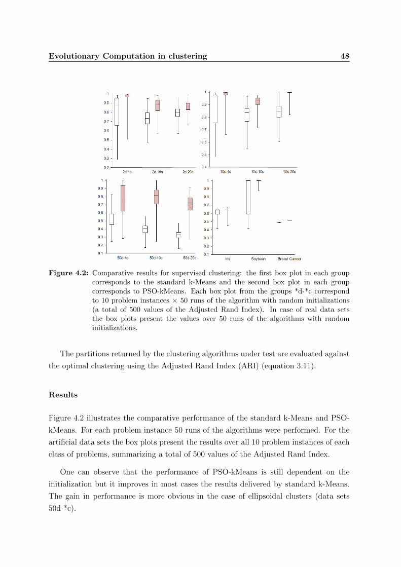
Evolutionary Computation in clustering 48
Figure 4.2: Comparative results for supervised clustering: the first box plot in each groupcorresponds to the standard k-Means and the second box plot in each groupcorresponds to PSO-kMeans. Each box plot from the groups *d-*c correspondto 10 problem instances × 50 runs of the algorithm with random initializations(a total of 500 values of the Adjusted Rand Index). In case of real data setsthe box plots present the values over 50 runs of the algorithms with randominitializations.
The partitions returned by the clustering algorithms under test are evaluated against
the optimal clustering using the Adjusted Rand Index (ARI) (equation 3.11).
Results
Figure 4.2 illustrates the comparative performance of the standard k-Means and PSO-
kMeans. For each problem instance 50 runs of the algorithms were performed. For the
artificial data sets the box plots present the results over all 10 problem instances of each
class of problems, summarizing a total of 500 values of the Adjusted Rand Index.
One can observe that the performance of PSO-kMeans is still dependent on the
initialization but it improves in most cases the results delivered by standard k-Means.
The gain in performance is more obvious in the case of ellipsoidal clusters (data sets
50d-*c).
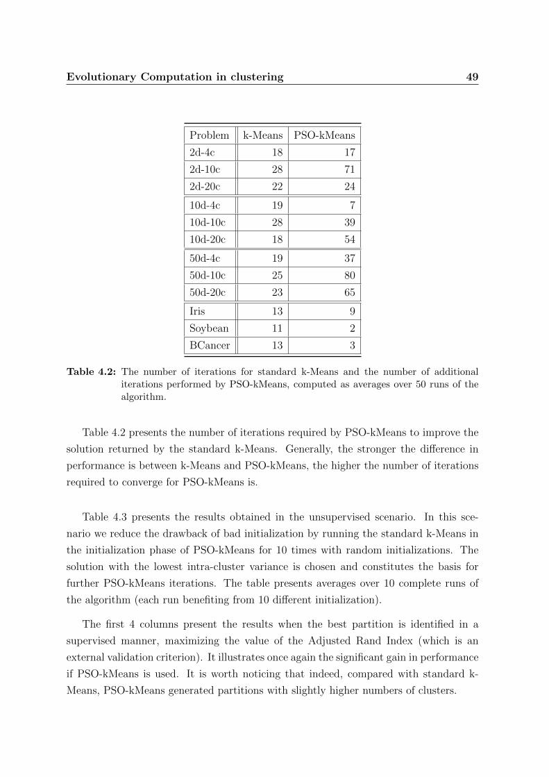
Evolutionary Computation in clustering 49
Problem k-Means PSO-kMeans
2d-4c 18 17
2d-10c 28 71
2d-20c 22 24
10d-4c 19 7
10d-10c 28 39
10d-20c 18 54
50d-4c 19 37
50d-10c 25 80
50d-20c 23 65
Iris 13 9
Soybean 11 2
BCancer 13 3
Table 4.2: The number of iterations for standard k-Means and the number of additionaliterations performed by PSO-kMeans, computed as averages over 50 runs of thealgorithm.
Table 4.2 presents the number of iterations required by PSO-kMeans to improve the
solution returned by the standard k-Means. Generally, the stronger the difference in
performance is between k-Means and PSO-kMeans, the higher the number of iterations
required to converge for PSO-kMeans is.
Table 4.3 presents the results obtained in the unsupervised scenario. In this sce-
nario we reduce the drawback of bad initialization by running the standard k-Means in
the initialization phase of PSO-kMeans for 10 times with random initializations. The
solution with the lowest intra-cluster variance is chosen and constitutes the basis for
further PSO-kMeans iterations. The table presents averages over 10 complete runs of
the algorithm (each run benefiting from 10 different initialization).
The first 4 columns present the results when the best partition is identified in a
supervised manner, maximizing the value of the Adjusted Rand Index (which is an
external validation criterion). It illustrates once again the significant gain in performance
if PSO-kMeans is used. It is worth noticing that indeed, compared with standard k-
Means, PSO-kMeans generated partitions with slightly higher numbers of clusters.

Evolutionary Computation in clustering 50
Problem Best ARI SW CritC
k-Means PSO-kMeans k-Means PSO-kMeans k-Means PSO-kMeans
ARI k ARI k ARI k ARI k ARI k ARI k
2d-4c 0.92 4.02 0.98 4.60 0.87 3.70 0.95 5.88 0.85 4.01 0.94 5.34
2d-10c 0.83 10.93 0.94 10.11 0.78 11.24 0.91 12.34 0.79 10.39 0.90 11.40
2d-20c 0.91 19.63 0.93 21.24 0.87 16.71 0.90 20.70 0.89 17.45 0.90 20.10
10d-4c 0.97 3.99 0.99 4.56 0.90 3.59 0.99 4.50 0.93 3.5 0.95 6.06
10d-10c 0.92 9.21 0.97 11.32 0.91 9.03 0.94 9.72 0.89 8.36 0.95 12.44
10d-20c 0.97 20.23 0.99 21.76 0.94 18.05 0.99 21.7 0.96 20.44 0.99 21.40
Table 4.3: Results for unsupervised clustering. For each data set and each algorithm, the ARIand the number of clusters are reported for three partitions: the partition withthe highest Adjusted Rand Index (ARI) score, the best partition under SilhouetteWidth (SW) and the best partition under criterion CritC.
Even when the partition is chosen using unsupervised criteria, PSO-kMeans still wins
the competition with standard k-Means. The Wilcoxon Signed-Rank non-parametric
test was applied for all pairs of ARI scores corresponding to (k-Means, PSO-kMeans)
under the same criterion. Where differences are significant (at the level 1%) the winner
is marked in bold.
All experimental results suggest that PSO-kMeans improves the performance of stan-
dard k-Means on all test cases. It achieves this, by forcing the standard algorithm to
obey the connectivity principle: neighboring data items should reside in the same cluster.
Moreover, the standard k-Means algorithm is sensitive to outliers: the cluster centroids
are biased if isolated data items exist because generally the mean is not a stable statistic
and extreme values affects it. PSO-kMeans is more robust to outliers which are attracted
towards dense regions and do not bias the position of the cluster centroids.
The complexity of a PSO-kMeans iteration is still linear in the number of data items.
However, the pre-processing time complexity is O(n2) as it is necessary to compute the
distances among data items.
As the experiments show, the new algorithm does not require parameter tuning to
increase performance when dealing with diverse datasets.

Evolutionary Computation in clustering 51
Problem PSO-kMeans k-Means PSO Single Average Complete Ward DBSCAN
Link Link Link
elongated 1 0.00 0.00 1 0.00 0.01 1 1
noise 1 0.80 0.93 1 1 1 1 1
unequal 1 0.84 0.86 1 1 0.10 1 1
overlapped 0.90 0.90 0.90 0.00 0.00 0 0.00 0.00
Table 4.4: The ARI computed for the datasets presented in Figure 2: our method(PSO-kMeans), standard k-Means, the clustering method proposed inCui et al.(2005)(PSO), 4 hierarchical algorithms and a density-based method.
4.2.4 Comparative study
The experimental section showed the superiority of our method over standard k-Means.
However, we would like to place our method in the wide context of clustering and there-
fore a comparative analysis with other state-of-the-art clustering methods is required.
To this goal, some problem instances imposing different challenges to clustering algo-
rithms are used: elongated clusters (4.3 a), data with noise(4.3 b), spherical clusters of
different volumes (4.3 c) and overlapped clusters (4.3 d). Table 4.4 presents the results
obtained by various algorithms.
Figure 4.3: Data sets imposing different challenges to clustering methods
Centroids-based methods
The standard k-Means and an existing hybridization of k-Means with PSO Cui et al.
(2005) are employed to study the behavior of centroids-based clustering methods relative

Evolutionary Computation in clustering 52
to PSO-kMeans which injects the connectivity principle into the representative-based
approaches for clustering.
Figure 4.4 presents the best partitions obtained with standard k-Means from multiple
runs. These partitions are identical to those obtained with the PSO algorithm presented
in (Cui et al. (2005)) which performs a global search in the space of possible initializations
for k-Means.
Figure 4.4: Results obtained with standard k-Means
The main drawback of the centroids-based methods becomes obvious: if clusters of
elongated shape or of various volumes are involved, these methods fail in retrieving the
correct partitions.
In case outliers are present in data and no pre-processing step is used to eliminate
them, the centroids are biased and erroneous partitions are delivered.
When the dataset contains spherical overlapped clusters the centroids-based methods
outperform other strategies.
Hierarchical methods
Usually, clusters of different shapes do not raise difficulties for hierarchical methods;
however, the result is highly dependent on the metric used to measure the similarity
between clusters.
For the dataset with elongated clusters, Single link and Ward’s method identify
correctly the two clusters. Average link and complete link deliver erroneous results as
shown in Figure 4.5.

Evolutionary Computation in clustering 53
Figure 4.5: Results for hierarchical algorithms on elongated data
In case of the dataset with clusters of various volumes, all hierarchical methods
performed well, except the Complete link variant.
All hierarchical algorithms identified the noise in case of the data set in figure 4.3 a
(noise).
In case of overlapped clusters, no hierarchical method was able to identify the clusters.
Density-based methods
After fine-tuning efforts, DBSCAN identified the clusters in case of the datasets 4.3a,b,c.
It failed to identify the overlapped clusters.
Discussion
Because our method takes into account the local structure in data and implements the
connectivity principle, it is able to identify clusters of different volumes and shapes.
Therefore, it identifies correctly the clusters for the datasets in figure 4.3 a and b,
behaving equally well to Single link, Ward’s method and DBSCAN and outperforming
all other tested techniques. PSO-kMeans outperforms not only the standard k-Means
algorithm. Tests were performed using a centroid method proposed in Cui et al. (2005)
which is also based on PSO. As explained in section 4.1, the existing methods based on
PSO or Genetic Algorithms behave like an upper bound for the standard k-Means: they
deliver (in the best case) the partition retrieved by a k-Means algorithm if the latter is
supplied with the best initialization.
Our method is still able to identify the clusters when outliers are present in data (the
dataset in figure 4.3 c). This behavior is due to the change in representation for the
outlier data items, which are attracted towards denser regions. Again, the performance

Evolutionary Computation in clustering 54
of PSO-kMeans is comparable to hierarchical methods and density based methods and
outperforms the centroids-based methods.
For the data set with overlapped clusters, the performance of our method is compa-
rable to that of the standard k-Means and significantly superior to that of hierarchical
methods and density-based methods. In contrast with the other test-cases, the dataset
in figure 4.3 d illustrates the positive effect of the centroid approach incorporated in our
method.
Benefiting from the global view over the data in addition to the connectivity prin-
ciple, the experiments show that our method is able to outperform the state-of-the-art
clustering methods or behaves equally-well in the worst case.
4.2.5 Concluding Remarks and Future Work
A hybridization of the standard k-Means algorithm with a technique from Swarm In-
telligence was proposed, with the aim of enhancing the performance of the traditional
clustering method. The new algorithm modifies the representation of the data items in
order to implement the connectivity principle for clustering. The changes in representa-
tion lead to changes in the distribution of distances between data items. Therefore, the
new algorithm can be easily extended to perform semi-supervised clustering. The addi-
tional information available in the form of similarity/dissimilarity pairwise constraints
can be easily incorporated in the PSO iterations to simulate metric learning along with
the clustering process. This hypothesis constitutes the subject of our future work.
4.3 Community detection in social networks
This section is concerned with a problem in information organization and retrieval within
Web communities [Breaban et al. (2009)]. Most work in this domain is focused on
reputation-based systems which exploit the experience gathered by previous users in
order to evaluate resources at the community level. The current research focuses on a
slightly different approach: a personalized evaluation system whose goal is to build a
flexible and easy way to manage resources in a personalized manner. The functionality
of such a model comes from local trust metrics which propagate the trust to a limited
level into the system and, finally, lead to the appearance of minorities sharing some

Evolutionary Computation in clustering 55
similar features/preferences. A modified PSO procedure is designed in order to analyze
such a system and, in conjunction with a simple agglomerative clustering algorithm,
identify homogenous groups of users.
4.3.1 Motivation
The World Wide Web stores great amounts of data. Any kind of resources can be
published by anyone: a diary published within a blog, a track that a user wants to share
with the others, a study that the author wants to make public. In this context, the
main problem is not the lack of good quality resources, but their retrieval, organization
and maintenance. This study is part of a recently proposed approach to improve the
performance of existing management systems within online communities. An online
community can be a forum, a group of blogs or other social system which allows users
to interact and to share resources.
The problem we tackle is related to the Web Collective Intelligence spectrum, where
many study directions can be envisaged. Much work is carried out nowadays in order
to design strategies to rate the resources or to build recommendation systems.
One example is Google Page Rank (A. Langville, C. Meyer, 2006) which, based on
some complex algorithms, assigns ranks to Web pages as a measure of their ”global
importance”.
In the case of recommendation systems, the shopping history and users’ charac-
teristics are being collected and based on this information the system makes proper
recommendations (e.g. Amazon, Netfix).
One active research direction is represented by the online communities who rely
on the mechanisms offered by trust and reputation systems. A trust and reputation
system exploit the users’ experience (resulted from the previous interactions) in order
to establish some user-user and user-resource evaluation/trust levels. In the literature
there are two categories of algorithms to calculate trust: global and local (also called
global trust metrics, respectively local trust metrics). In Massa and Avesani (2007) the
advantages and the drawbacks of both approaches are presented.
Currently, most of the approaches focus on the first category. These algorithms aim
at quantifying the importance of an user/resource at the community level. These ap-

Evolutionary Computation in clustering 56
proaches assume that all the users in the community have similar ideas. This assumption
lead in the extreme case to a phenomenon described as ”tyranny of the majority”.
Few approaches are concerned with the development of local trust metrics [Golbeck
(2005); Massa and Avesani (2007); Ziegler (2005)]. The local trust metrics propagate
trust in a limited manner. Each user is connected only to a subset of users/resources.
In the extreme case, a segmentation of the society into isolated groups may be achieved.
The challenge consists in designing a system which balances out the two extreme
situations.
The work presented in this section is conducted within a recently proposed system
based on local trust mechanisms Alboaie (2008). A general model of calculating trust
and reputation was proposed, which allows a user from the community to have a per-
sonalized view on the system. Interesting elements of analysis of these models concern
not just users but also groups of users. As shown in the following sections, we focus our
research on the techniques which lead to obtaining relevant groups of users, so that the
personalized group vision provided by the model to be accurate as well.
The problem is strongly related to community finding within social networks; this is
a topic of great interest, intensively studied in the last years. The problem is formally
defined as a graph problem: identify groups of vertices within which connections are
dense, but between which connections are sparser. Existing methods are based on divi-
sive strategies which compute centrality indices to find community boundaries [Girvan
and Newman (2002)] or make use of the hierarchical clustering scheme [Clauset et al.
(2004)]. Recently, evolutionary algorithms were proposed to tackle this problem [Gog
et al. (2007)]. The method proposed in this section, although designed for the particular
case of local trust networks, can be applied for general social graphs as well.
Section 4.3.2 describes the trust and reputation system and introduces the problem
we analyze: the detection of homogenous groups of users. In section 4.3.3 this problem
is analyzed and a solution which is based on Particle Swarm Optimization is described.
Section 4.3.4 presents the experimental results and section 4.3.6 concludes with a brief
discussion on the results and some future directions.

Evolutionary Computation in clustering 57
4.3.2 The engine ratings of a trust and reputation system
In [Alboaie (2008)] a personalized evaluation system was proposed, whose goal is to build
a flexible and easy way to manage resources in a personalized manner. The purpose of
the proposed model is to offer a flexible mechanism to filter irrelevant resources for users.
The system is designed to be used in an online community. Therefore, the main
constituents are the users and the resources (their definition is made according to the
definition given by T. Berners-Lee, 1998). A relation worth : U×U → (0, 5] over the set
of users is introduced: it is a measure of the level of trust that a user associates to any
other user; simplified, worth(Ui, Uj) may quantify the interest expressed by user i for the
resources posted by user j. The users assign explicitly one another some ratings which
are expressed as real numbers in the interval (0,5]. The five unit-length sub-intervals
represent five different levels of trust ranging from ”useless/spam” to ”exceptional”.
These values must be used further by the system in order to filter relevant resources for
users’ queries. Since one user rates explicitly only a subset of the users in community,
an algorithm was proposed which propagates these evaluations over the set of users and
computes implicit ratings. Such algorithms are called local trust metrics within the Web
community.
The current research is focused on identifying homogenous groups of users in this
system. For large communities, this analysis is highly motivated:
• Exploratory data analysis by means of clustering is a coherent approach for gath-
ering a general view of the system and even to get insights into its dynamics;
• For small communities (small worlds) the computation of the rating’s nucleus gives
a proper solution of modeling. When communities with a great number of members
are involved, the computation cost is very high. As a solution, an extension of the
existing model may be introduced. The idea consists of grouping the members
of the community into homogenous groups; these groups are further integrated as
entities which can express their level of trust among them and can have a reputation.
Further, each user will assume the trust statements of the group it belongs to.
Two types of groups can be formed within the presented system: explicit groups and
implicit groups. Creating explicit groups is a frequently met phenomenon in the present
online communities. The explicit groups are created by users and anyone can create,
adhere to or leave such a group.

Evolutionary Computation in clustering 58
Figure 4.6: The model extension: ratings associated to groups
The implicit groups are to be created by the system based on the user-user evalu-
ations. In this case, using automatic unsupervised techniques, clusters of users will be
obtained. Users from the same cluster are supposed to share the same points of view on
the community/resources. Consequently, the resources may be clustered in relation to
the users who added them in the system. This way of grouping allows the establishment
of a quick correspondence between the users clusters and the resources clusters. The
motivation for choosing to create such groups is simple: once user A rates highly user B,
it would make sense that at some moment it will be interested in the resources posted by
user B. Therefore, we get to the level when the system implicitly recommends resources
to the user.
4.3.3 The algorithm
This section identifies the main challenges raised by the problem at hand: retrieve
homogenous groups of users based on the expressed preferences. The solution, based on
the Swarm Optimization paradigm is detailed.
Problem statement
The clustering problem is generally formulated in terms of an input consisting of n
data items, each described by m numerical attributes. An alternative representation
is a n × n symmetric matrix expressing the similarity between pairs of data items.
Unfortunately, none of these representations and consequently no existing clustering
algorithm are straightforward applicable in our case.
In our system, a data item corresponds to a user; each user can be characterized by
a vector of length 2n containing the ratings it gives to other users in the system and

Evolutionary Computation in clustering 59
the ratings it receives. Performing clustering based directly on these features would be
unfeasible, mainly due to the following drawbacks:
• High dimensionality: the size of the feature space is a multiple of the size of the
data set;
• Defining a metric over such a feature space is not straightforward. The similar-
ity between 2 users A and B should be computed with regard to the following
assumptions:
– personal preferences: A is similar to B if A and B rate in the same manner the
users within the system;
– obtained ratings: A is similar to B if they are rated similarly by a large group
of users;
– direct interactions: a high rating given by user A to user B expresses the affinity
of user A for user B and therefore, the tendency for user A to adhere to user
B’s cluster.
Any existing metric applied to the mentioned feature vectors space would consider
the first two clustering criteria but neglect the most important one - the third
criterion.
In previous work, groups were identified within this system using hierarchical clustering
Alboaie and Barbu (2008). Usually, the users evaluate and are evaluated by a different
number of users. In order to reduce dimensionality, the feature vector for user A is
constructed only over the users it interacts with: the users A rates and the users which
rate user A. Therefore, the feature vectors have different lengths and a special kind of
distance metric derived from the Hausdorff metric for sets is used. Although the results
are encouraging, this approach ignores the third criterion detailed above.
In order to eliminate the above mentioned drawbacks, we designed a clustering pro-
cedure which is based on the third criterion, incorporates the second criterion explicitly
and achieves the first one implicitly. The users are modeled as particles in a PSO algo-
rithm; they move within a two-dimensional space creating a topology that reflects the
affinities among them. A simple agglomerative clustering procedure implementing the
connectivity principle is then applied to cluster the points in the two-dimensional space
using the Euclidean metric: any two points at distance lower than a given threshold will
share the same cluster.

Evolutionary Computation in clustering 60
The embedding procedure
A modified version of PSO is used in our work in order to obtain a two-dimensional
representation of the community of users, representation which reflects the interac-
tions/affinities among them. This two-dimensional embedding can be used to visual-
ize the community from a user-oriented perspective: users which give high ratings one
another, expressing in this way some common views, will be located close in the two-
dimensional Euclidean space. Performing further a simple clustering procedure in this
Euclidean space, somewhat homogenous groups of users can be easily identified.
In our approach, the users become particles in a swarm, within a two-dimensional
Euclidean space. The mapping procedure is inspired from the PSO algorithm but two
essential modifications were introduced.
The motion rules are not governed by a fitness function; the expressed preferences in
form of ratings the users give one another guide individual trajectories towards a stable
configuration. This is one essential deviation from the basic PSO algorithm: the particles
are not assigned unique, unanimously accepted fitness values, based on the position they
occupy in the search space. Each particle has its own view on the swarm and its personal
”goals”, which are expressed as personalized fitness assignments to other particles. There
is no global best particle in the swarm or in a subpart of the swarm, but one distinct best
particle for each member of the swarm. However, these personalized fitness evaluations
do not counteract the emergence process the general Swarm Intelligence techniques are
based on: simple rules describing individual trajectories lead to novel and coherent
structures, patterns and properties during the process of self-organization (Goldstein,
1999).
Another deviation from the PSO basic scheme is a change in motion rules. Except
the attraction towards the best particle, the remaining two rules are re-defined. The
procedure is detailed below.
In an initialization step, each user is assigned a randomly-generated point in a two-
dimensional space; these points are to be further considered as position vectors of the
particles in a swarm. Then, an iterative process aims at organizing the particles, such
that the users with ”strong interactions” will be matched to close points in the Euclidean
space. In the sequel, the terms particle/user are interchangeable: both denote individuals
in a swarm, characterized by a position vector in a two-dimensional space and a velocity
vector; an n × n matrix stores the pair-wise affinities in the form of real numbers in
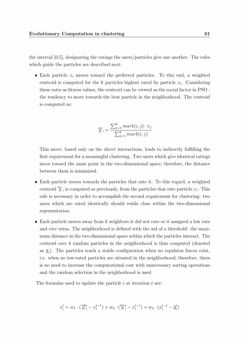
Evolutionary Computation in clustering 61
the interval [0,5], designating the ratings the users/particles give one another. The rules
which guide the particles are described next:
• Each particle xi moves toward the preferred particles. To this end, a weighted
centroid is computed for the k particles highest rated by particle xi. Considering
these rates as fitness values, the centroid can be viewed as the social factor in PSO -
the tendency to move towards the best particle in the neighborhood. The centroid
is computed as:
−→g i =
∑kj=1mark(i, j) · xj∑kj=1mark(i, j)
This move, based only on the direct interactions, leads to indirectly fulfilling the
first requirement for a meaningful clustering. Two users which give identical ratings
move toward the same point in the two-dimensional space; therefore, the distance
between them is minimized.
• Each particle moves towards the particles that rate it. To this regard, a weighted
centroid←−g i is computed as previously, from the particles that rate particle xi: This
rule is necessary in order to accomplish the second requirement for clustering: two
users which are rated identically should reside close within the two-dimensional
representation.
• Each particle moves away from k neighbors it did not rate or it assigned a low rate
and vice versa. The neighborhood is defined with the aid of a threshold: the maxi-
mum distance in the two-dimensional space within which the particles interact. The
centroid over k random particles in the neighborhood is thus computed (denoted
as gi). The particles reach a stable configuration when no repulsion forces exist,
i.e. when no low-rated particles are situated in the neighborhood; therefore, there
is no need to increase the computational cost with unnecessary sorting operations
and the random selection in the neighborhood is used.
The formulas used to update the particle i at iteration t are:
vti = w1 · (−→g ti − xt−1
i ) + w2 · (←−g ti − xt−1
i ) + w3 · (xt−1i − gti)

Evolutionary Computation in clustering 62
xti = xt−1i + wmax · vti
The parameters and the stopping criterion are empirically determined.
The PSO procedure is followed by a single link agglomerative procedure which can
be stopped when a fixed number of clusters is achieved or when the distance between
clusters exceeds some threshold. Since the two-dimensional representation obtained with
PSO can be visually analyzed, the number of clusters can be specified. Anyway, the use
of k-Means algorithm is not recommended: as shown in the experimental section, the
resulted clusters have different shapes and volumes and even some isolated points may
be obtained.
4.3.4 Experiments
Parameters settings
In order to obtain a first empirical setting of PSO parameters, small problem instances
were created; the resulted two-dimensional maps are validated by analyzing the ratings
table. One such instance is represented in Figure 4.7; two maps created using different
initializations are illustrated in Figure 4.8.
Figure 4.7: The graphs representing a community of 14 users; A: the graph containing theexplicit ratings; B: the graph containing both explicit and implicit ratings; thecontinue arcs represent the explicit ratings and the dashed arcs the implicit rat-ings.
The parameters values were set as follows:

Evolutionary Computation in clustering 63
Figure 4.8: Two different mappings corresponding to different initialization
• w1 = 0.5; the direction of any particle is dictated mainly by the particles it rates;
• w2 = 0.15; a small value for this parameter enforces each particle to stay relatively
close to the particles it was rated by;
• w3 = 0.25; a moderate repulsion force active below a threshold (set to 1) which
defines the neighborhood of a particle, determine unrelated particles to stay far
away from one another; the repulsion centroid is computed over at most k = 5
neighbors.
• wmax = 0.15.
A threshold concerning the ratings was used: only ratings greater than 2 denote
strong affinities and consequently attraction forces.
For small instances, as the one illustrated in Figure 4.7, the algorithm reaches a
stable configuration after 50 iterations. For larger communities, more iterations are
required until a stable configuration is reached. As a halting criterion, an average over
velocities vectors may be computed and compared to a scalar threshold: small velocities
correspond to stable configurations. We look for the number of iterations after which
no major changes on the two-dimensional map are observed.
As one can observe in Figure 4.8, the initial configuration influences the orientation
of clusters and, to some extent, their relative positions; on the other hand, the same
clusters are detected in repeated runs (different initializations) and within each cluster
the components are arranged under the same topology.

Evolutionary Computation in clustering 64
These first empirical results are illustrative for the convergence of the algorithm:
repeated runs involving different initial configurations lead (after a limited number of
iterations) to similar stable configurations. The similarity between configurations is
measured in terms of detected clusters: the number of clusters, the constituents of
each cluster and even the shape of the clusters. All these elements illustrate topology
preservation.
A more in-depth analysis is necessary in order to verify the agreement between the
resulted mapping and the graph of ratings. In Figure 4.8, due to the single-directional
high ratings, one linear cluster is formed over particles 1,3,8,11 and 10. Particles 5 and
13 end-up close together due to bi-directional (reciprocal) high ratings; following them at
greater distance particles 6 and 7 are situated. Due to the lack of any evaluations/ratings,
particles 2, 9 and 14 are isolated in different regions of the map.
Data generator
Once empirically tuned on synthetic small data sets, the method needs to be tested on
larger (real) data sets. Unfortunately, existing systems/comunities do not make public
the data and no benchmark is available. Previous studies on local trust metrics report
some tests on data extracted from Epinions community (Massa and Avesani (2007)).
Ziegler (2005) created synthetic data for tests.
In order to simulate real communities, we designed a somewhat complex data genera-
tor. It takes as input an xml file which can be customized to generate different categories
of explicit evaluations. The following parameters are introduced:
• users - the number of users in the community;
• goodUsers - an approximation of the number of ”good” users in the community;
that is, the number of users who receive the majority of good evaluations;
• minMarksCount - the minimum number of evaluations realized by an entity; for a
better observation of the dynamics of spreading the trust each user must interact
with the comunity.
• goodMarksThreshold - the threshold which separates the good evaluations from
the worse ones; this parameter is further used in the clustering procedure;

Evolutionary Computation in clustering 65
• userRatingsDensity - a percentage which represents the density of the community’s
network: how many explicit evaluations are made in the system (from a total of n2
possibilities).
• goodUserMaxDivergence - a percentage representing the number of bad marks that
can be awarded to an user already designated as being ”good”.
Experimental settings
As shown in section 4.3.4, the final mapping is strongly dependent on the initial configu-
ration. Due to random initializations, the stability of the method must be investigated.
This analysis is compulsory for probabilistic heuristics and generally consists in comput-
ing the variance of solutions obtained in repeated runs.
As the main goal of the method is to identify meaningful clusters, we study the
stability of the method with regard to the detected clusters.
On small problem instances, as the one presented in section 4.3.4, the results are easy
to analyze visually. For larger problem instances the analysis we conducted consists of
the following steps:
• run several times PSO-mapping on the same problem instance with random initial-
izations;
• apply a deterministic clustering algorithm on each mapping;
• measure the similarity between the clustering solutions (the partitions) and com-
pute an average.
To perform clustering in the two-dimensional space we designed a single link agglom-
erative clustering procedure; the procedure stops when the distance between classes
exceeds a given threshold.
As measure of similarity between two partitions we used Adjusted Rand Index.
Problem instances were generated for different parameters of the data generator.
Tests were performed on problem instances consisting of 20, 50 and 100 users.
In each case, 5 problem instances were generated; PSO and the subsequent clustering
procedure were applied five times on each problem instance. The similarity measure

Evolutionary Computation in clustering 66
was computed for each pair of the resulted partitions and the average over all pairs is
reported.
Experimental results
Table 4.5 presents the experimental results over several classes of problem instances gen-
erated for different settings of the data generator. The parameters of the data generator
are specified in the following order: users-goodUsers-userRatingsDesity. The minimum
number of evaluations given by a user was set to 1. In all experiments the value for
goodUserMaxDivergence was set to 10% ; this defines a user as beeing ”good” if more
than 90% of the ratings it receives are greater than goodMarksThreshold parameter
value.
As the main purpose of the generator is to simulate real online communities, the
average number of obtained clusters is computed in order to study their dynamics.
PROBLEM INSTANCE ARI NUMBER OF
CLUSTERS
20-15-0.3 0.9611 3
20-10-0.3 0.8553 8
50-35-0.5 0.9376 3
50-20-0.5 0.8853 4
50-35-0.3 0.7969 4
50-20-0.3 0.6872 7
50-35-0.1 0.7694 12
50-20-0.1 0.8753 16
100-65-0.1 0.7832 14
100-50-0.1 0.7634 17
100-35-0.1 0.6323 22
100-35-0.3 0.8251 4
Table 4.5: Average Adjusted Rand Index and the average number of clusters for differentclasses of problem instances
The high ARI values reported in Table 4.5 indicate coherent/similar partitions ob-
tained at repeated runs, which further suggest stable and similar mappings produced

Evolutionary Computation in clustering 67
by the PSO procedure. Anyway, the mapping algorithm is influenced to some extent
by the initial configuration and the stability of the algorithm seem to depend on the
parameters of the problem.
As expected, the stability of the mapping procedure based on PSO generally de-
creases with the size of the problem, as the number of possible configurations grows
exponentially.
One important parameter which acts in the opposite way is the ratings density. When
there are many evaluations in the system, complex interactions dictate the dynamics
of the system and, consequently, of the swarm in the mapping procedure. The PSO
particles are subjected to more restrictions regarding their motion in the two-dimensional
space. To reach a stable configuration a larger number of iterations is needed but the
outputs are less sensitive to the initial configuration.
Increasing the number of good users in the system, some cluster nucleus appear and
well-defined clusters are to be formed. Consequently, the particles concentrate in dense
clusters where the repulsion forces are minimized and the algorithm is more stable for
such configurations.
Some general conclusions regarding the influence of the mentioned parameters on the
number of clusters may be drawn.
The number of good users in the system has a great influence on the number of
clusters. In order to coexist more good users in the system, several users have to rate
them high. This lead to few larger clusters.
The same influence is observed for the userRatingsDensity parameter: few explicit
ratings in the system determine sparse configurations and consequently, many small
clusters.
The method can be used to study further the dynamics of the system. Many scenarios
can be imagined. For example, one interesting case study concerns the impact of a
new user’s evaluations on the system. The structure of clusters and, furthermore, a
visualization of the embedding produced with the proposed algorithm are useful tools
for such analysis.

Evolutionary Computation in clustering 68
4.3.5 Applications to social networks
With minimal modifications, the method can be applied to identify communities in social
networks.
To study its performance, the American Football data set introduced in Girvan and
Newman (2002) is used. The data set can be represented as a graph consisting of
115 nodes and 616 edges: the nodes represent football teams and the edges represent
regular season games between the two teams they connect. The teams are divided into
11 ”conferences”. The teams play an average of about 7 intra-conference games and 4
inter-conference games.
We apply the PSO/clustering method described previously with the aim of identifying
the ”conferences”. In order to benefit from the previous scenario, the original problem
graph is transformed into a weighted digraph: each edge is replaced by two opposite
arcs and equal weights are assigned to all arcs. Under this representation, the second
term in the PSO-mapping algorithm is identical to the first term and therefore, may be
eliminated. Equal weights (0.5) were set for the two remaining terms. A run for the
PSO-mapping procedure consists of 500 iterations; the subsequent single link clustering
procedure is stopped when the cluster inter-distance exceeds 0.75 (3/4 reported to the
activation threshold for the repulsion force which is set to 1).
In order to compare the results obtained by our method with the actual constitution
of the ”conferences”, an average over 10 runs for the Adjusted Rand Index was computed;
the obtained value of 0.7763 indicate a close match between the generated partitions and
the actual partition. The divergence is mainly due to a higher number of detected clusters
(15 on average) and only to a little extent is due to wrong allocations. To illustrate
this, the mapping and the resulted clusters for a low-performance run (ARI=0.71) are
presented in Figure 4.9.
The mapping takes the regular form of rectangular lattice. Clusters 0, 1, 4 and
8 are matched perfectly to the real partition. Each one of the actual classes 2, 3, 6
and 9 are divided by our mapping into two adjacent clusters. One team from class
11 was misclassified. Regarding class 7, along with the correct members, other teams
were incorrectly added; the resulted cluster is sparser, suggesting incorrect matching.
Members of classes 5 and 10 were incorrectly mixed.
The obtained results indicate that the presented method is an appropriate approach
for community detection in social networks.

Evolutionary Computation in clustering 69
Figure 4.9: Mapping for the American College Football network; the teams are representedas points in the two-dimensional space; well-defined clusters are identified; theclusters are specified in brackets followed by the actual membership of the teams.
4.3.6 Concluding Remarks and Future Work
The main aim of this section is to propose a method to get insights into the structure and
dynamics of online communities which operate on mechanisms of trust. An embedding
of the community into a two-dimensional Euclidean space, which reflects affinities among
users, allows by means of simple clustering procedures to identify natural groups. As a
basis of this method, Particle Swarm Optimization is employed: the simple individual
rules which lead to self-organization in complex systems (the emergence process) fit
perfectly to this problem.
The identification of cohesive communities by means of clustering procedures is a
key process in social network analysis. The current approach can be applied to general
social graphs as well.
As future work, the mapping/clustering procedure will be extended by introducing
direct resources evaluations in the current local trust network.
4.4 Genetic-entropic clustering
This section addresses the clustering problem given the similarity matrix of a data
set (Breaban et al.). By representing this matrix as a weighted graph we transform
this problem into a graph clustering/partitioning problem which aims at identifying
groups of strongly inter-connected vertices. We define two distinct criteria with the aim

Evolutionary Computation in clustering 70
of simultaneously minimizing the cut size and obtaining balanced clusters. The first
criterion minimizes the similarity between objects belonging to different clusters and is
an objective generally met in clustering. The second criterion is formulated with the aid
of generalized entropy. The trade-off between these two objectives is explored using a
multi-objective genetic algorithm with enhanced operators. As the experimental results
show, the Pareto front offers a visualization of the trade-off between the two objectives.
4.4.1 Graph clustering
In clustering the data items can occur either as tuples, which are ordered sequences of
categorial or numerical values, or as simple objects for which only pairwise similarities
or dissimilarities are provided. The first kind of layout offers more information and is
suitable to any clustering algorithm once an appropriate metric is chosen. The second
kind cannot be supplied to any clustering algorithm (i.e. k-Means), but eliminates
one difficult step in unsupervised clustering analysis - the definition of an appropriate
similarity measure. The transition from the first kind of layout to the second is trivial
when a similarity function is defined; the backward transition can be performed to some
extent using multi-dimensional scaling algorithms.
When the similarity matrix of a dataset is given, a straightforward representa-
tion of the problem instance is a weighted graph, having the objects as vertices and
weighted edges expressing the similarity between objects. This leads to a graph cluster-
ing/partitioning problem which aims at identifying groups of strongly inter-connected
vertices.
There exist several formal definitions of graph clustering, depending on the practical
application and domain where the problem originates. These variations are reflected in
the graph structure and in the objectives aimed to be optimized. A survey on various
problem definitions and methods for graph clustering is presented in Schaeffer (2007).
The graph clustering problem this section addresses has important applicability in
VLSI circuit design, image processing, and distributing workloads for parallel computa-
tion. A formal definition is given next.
A similarity space is a pair (S,w), where w : S × S[0, 1] is a function such that
(i) w(s, t) = w(t, s) for every t, s ∈ S;
(ii) w(s, s) = 1 for every s ∈ S.

Evolutionary Computation in clustering 71
A similarity space (S,w) can be regarded as a labeled graph G = (S,E,w), referred to
as the similarity graph, where the set of edges E is defined as
E = (xi, xj) | xi, xj ∈ S and w(xi, xj) > 0.
In other words, an edge exists between two vertices only if they have a positive similarity.
If S = x1, ..., xn is a finite set the dissimilarity w is described by a symmetric
matrix W ∈ Rn×n, where wij = w(xi, xj) for 1 ≤ i, j ≤ n.
A k-way clustering of a finite similarity space (S,w) is a partition κ = C1, . . . , Ckof S. The sets C1, . . . , Ck are the clusters of κ. We seek a k-way partition of S, κ such
that
(i) the cut size (i.e. the sum of weights of edges between clusters in the similarity
graph) is minimal, and
(ii) |Cp| ≈ |Cq|, for 1 ≤ p, q ≤ k, which means that the sizes of the clusters are as equal
as possible.
The first objective is generally met in any clustering problem: the elements belonging to
different clusters should be dissimilar. In network applications this would correspond to
minimizing the communication time. The second objective expresses a load balancing
constraint, inherent in network applications.
This multi-objective problem was intensively addressed in literature in the last thirty
years. One of the earliest approaches is the method obtained by Kernighan and Lin
(1970) which refines a given (randomly generated) partition in a greedy manner by
reallocating pairs of nodes between clusters; like all greedy optimizers, this is a local
improvement algorithm. Several improvements with regard to time complexity were
later proposed. The most used methods are recursive algorithms: in a first step a two-
way partitioning is obtained after which, each of the clusters is bisected to obtain a
four-way partitioning and the process continues until the desired number of clusters
is reached. Recursive spectral bisection algorithms (see Simon (1991)) are known to
deliver good solutions but at high computational cost because they require eigenvector
computations.
To deal with large graphs, multilevel algorithms were proposed. They consist ba-
sically of three phases: coarsening, partitioning and uncoarsening. In the coarsening
phase the graph is compressed by successively collapsing nodes. A partitioning proce-

Evolutionary Computation in clustering 72
dure (such as the one obtained by Karypis and Kumar (1998) or a spectral method
presented by Barnardand and Simon (1993)) is applied on the coarsened graph. In the
uncoarsening phase, a partition is built for the original graph by assigning the collapsed
nodes to the same cluster; a costless refining phase may be used at this level.
An extensive state-of-the-art of the methods and comparative studies can be found
in Fjllstrm (1998), Karypis and Kumar (1998) and Alpert (1998).
Because of the multi-objective nature of the problem, we tackle the graph partition-
ing problem with a multi-objective genetic algorithm with enhanced operators. The
benefits of such an approach are obvious: instead of delivering a single solution, a set
of several non-dominated solutions approximating the Pareto front is returned. As the
experimental results show, the Pareto front offers a visualization of the trade-off be-
tween the two objectives; the shape of the Pareto front offers valuable information for
the identification of the optimum solution.
The remaining of this section is structured as follows. Section 4.4.2 examines the two
objectives which have to be optimized as stated in the problem definition. Section 4.4.3
provides a brief survey on the genetic algorithms for clustering with an emphasis on the
multi-objective formulation; the representation and the operators we used are detailed.
Section 4.4.4 presents experimental results.
4.4.2 A multi-objective formulation
Let κ = C1, . . . , Ck a clustering of the objects of the set S = x1, . . . , xn. The matrix
X ∈ Rn×k defined by
xip =
1 if xi ∈ Cp,
0 otherwise,
represents the clustering κ. Note that each row of this matrix contains a single 1 and
that the total number of 1 entries equals the number n of elements of the set S.
The matrix Y = X ′X ∈ Rk×k is given by
ypq =n∑i=1
x′pixiq =n∑i=1
xipxiq (4.2)

Evolutionary Computation in clustering 73
for 1 ≤ p, q ≤ k. Since any two clusters Cp, Cq are disjoint, this is a diagonal matrix. Its
diagonal elements are ypp = |Cp| for 1 ≤ p ≤ k.
Let G = (S,E,w) be the similarity graph of S defined as an undirected graph having
S as its set of vertices. The symmetric matrix W ∈ Rn×n is defined by
wij =
w(si, sj) if i 6= j,
1 if i = j,
for 1 ≤ i, j ≤ n.
Let Z = X ′WX ∈ Rk×k. We have
zpq =n∑i=1
n∑j=1
x′piwijxjq =n∑i=1
n∑j=1
xipwijxjq
for 1 ≤ i, j ≤ n. Therefore, for the distinct clusters Cp, Cq, zpq is precisely the value of
cut(Cp, Cq). Note also that
zpp =n∑i=1
n∑j=1
xipwijxjp
equals the sum of the similarities between the objects of the clusters Cp. Clearly, to
achieve maximal intra-clustering cohesion and minimal inter-clustering dissimilarity it
is necessary that the trace of the matrix Z (that is, the sum of the diagonal elements of
Z) to be maximal and the sum of the off-diagonal elements of Z to be minimal,
Since Z is a non-negative matrix, its norm ‖ Z ‖1=∑k
p=1
∑kq=1 |zpq| coincides with
the sum of its elements. Moreover, ‖ Z ‖1=∑n
i=1
∑nj=1 wij and is constant for a given
similarity matrix W , regardless of the clustering X. Therefore, the total weight of the
inter-cluster cuts equals ‖ Z ‖1 −trace(Z) and minimizing it is equivalent to maximizing
the total within clusters similarity which is given as trace(Z).
We use a novel approach to insure that the clusters of κ are balanced. To this
end, we use the generalized entropy of partitions of finite sets (see Simovici and Djeraba
(2008)).

Evolutionary Computation in clustering 74
For a partition κ = C1, . . . , Ck of a set S and a number β > 1, the β-entropy is
defined by
Hβ(κ) =1
1− 21−β
(1−
k∑p=1
|Cp||S|
β).
Note that limβ→1 Hβ(κ) = −∑k
p=1|Cp||S| log2
|Cp||S| . In other words, the Shannon entropy is
a special case of the generalized entropy.
An important special case of the entropy is obtained for β = 2. We have
H2(κ) = 2
(1−
k∑p=1
|Cp||S|
2),
and this is the well-known Gini index, gini(κ) used frequently in statistics.
The largest value of Hβ(κ) is obtained when κ consists of singletons, that is, when
k = n and κ = si | 1 ≤ i ≤ n and is Hβ(κ) = 11−21−β
(1− |1|
|S|β−1)
; the least value
of Hβ(κ) is obtained for κ = S and equals 0.
For a prescribed number k of blocks (where k is a divisor of |S|), the maximum value
of Hβ(κ) corresponds to a partition having blocks of equal sizes. If k is not a divisor
of S, then the more uniform the sizes of the cluster, the larger is the value of Hβ(κ).
This indicates that maximization of the entropy can be used as a criterion for ensuring
the uniformity of the cluster sizes. We will use the Gini index of κ because it presents
certain computational advantages as shown next.
Theorem 4.4.1 Let κ = C1, . . . , Ck a clustering of the objects of the set S =
x1, . . . , xn and let X ∈ Rn×k be the characteristic matrix of the clustering. We have
gini(κ) = 2(1− trace(X ′XX ′X)).
Proof. The definition of the matrix Y implies trace(X ′XX ′X) = trace(Y 2). Since Y
is a diagonal matrix, we have
trace(Y 2) =k∑p=1
|Cp|2

Evolutionary Computation in clustering 75
by Equality (4.2). Thus,
gini(κ) = 2
(1−
k∑p=1
|Cp||S|
2)
= 2(1− trace(Y 2)) = 2(1− trace(X ′XX ′X)).
Thus, two objectives can be used to find a balanced k-clustering κ:
(i) minimization of the total cut of the clustering partition, which amounts to mini-
mization of
f1(X) =‖ Z ‖1 −trace(Z) =‖ X ′WX ‖1 −trace(X ′WX) (4.3)
(ii) maximization of cluster uniformity, which is equivalent to the maximization of the
Gini index of κ, or to the minimization of
f2(X) = trace(X ′XX ′X) (4.4)
We seek X subjected to the conditions xip ∈ 0, 1 for 1 ≤ i ≤ n and 1 ≤ p ≤ k.
Depending on the aspects we need to emphazise in the clustering we can use a convex
combination of these criteria:
Φa(X) = a f1(X) + (1− a) f2(X)
= a (‖ X ′WX ‖1 −trace(X ′WX)) + (1− a) trace(X ′XX ′X),
where a ∈ [0, 1].
To simultaneously minimize criteria f1 and f2, also a non-linear combination can be
used:
Ψ(X) =f1(X)
n2 − f2(X)=‖ X ′WX ‖1 −trace(X ′WX)
n2 − trace(X ′XX ′X). (4.5)
The criterion Ψ(X) measures the average link between clusters, because the denom-
inator is proportional with the number of pairs of items that occur in distinct clusters.

Evolutionary Computation in clustering 76
4.4.3 The algorithm
We use a genetic algorithm (GA) to deal with the graph clustering problem, because
such algorithms provide a good exploration of the search space and are able to deliver
high-quality solutions.
Real-world problems necessitate most of the times the optimization of several con-
flicting objectives. Usually, this is achieved by combining the objectives into a single
function. However, some objectives may be more important than others for a given prob-
lem and their relative importance cannot be established beforehand. Multi-objective
GAs optimize simultaneously several objectives and return a set of non-dominated solu-
tions which approximate the Pareto front. For a problem involving m objectives denoted
with fi, 1 ≤ i ≤ m which have to be minimized, a solution x is dominated by a solution
x∗ if
fi(x∗) ≤ fi(x), ∀i = 1..m, and ∃1 ≤ j ≤ m s.t. fj(x
∗) < fj(x).
The Pareto optimal set of solutions X∗ consists of all those solutions for which no
improvement in an objective can be made without a simultaneous worsening in some
other objective. In other words, the Pareto front consists of all solutions that are not
dominated by any other solution.
The multi-objective scheme we use to tackle the graph clustering problem is PESA-II
obtained by Corne et al. (2001). The algorithm maintains two populations of solutions.
An external population stores mutually non-dominated clustering solutions, which cor-
respond to different trade-offs between the two objectives. At each iteration an internal
population is created by selecting chromosomes from the external population. This se-
lection phase takes into account the distribution of solutions across the two objectives
by maintaining a hypergrid of equally sized cells in the objective space. The solutions
are selected uniformly from among the populated niches such that highly populated
niches do not contribute more solutions than less populated ones. After selection, the
crossover and mutation operators are applied within the internal population. The exter-
nal population is updated by joining the two populations and eliminating the dominated
solutions. The general scheme of the algorithm is presented in Algorithm 4.10.
This multi-objective algorithm was previously used by han in unsupervised clustering
(when the number of clusters is not fixed and evolve during search) with very good
results. The objectives they optimized were connectivity and the within-cluster deviation

Evolutionary Computation in clustering 77
Figure 4.10: PESA-II
Initialize IP (internal population)Evaluate IPInitialize EP (external population) to include all mutually
non-dominated solutions from IPwhile halting condition not met do
delete the current content of IPfill IP with individuals selected uniformly among the niches from EPapply crossover and mutation in IPEvaluate IPUpdate EP
end while
and because the number of clusters was allowed to vary, a different representation and
consequently different operators were used.
The straightforward representation of a solution for the partitioning problem is a
string, encoding the cluster membership of each data item. This is the representation
used in our GA: an individual is a string of length n (the number of vertices in the
graph), taking values in the set 1, . . . , k, where k is the number of clusters.
If the standard operators would be used, this encoding would suffer from several
drawbacks like redundancy and invalidity and would determine a slow convergence of
the algorithm. However, due to the multi-objective scheme used and the new operators
we propose, this drawbacks are eliminated.
In the initialization phase a minimum spanning tree (MST) is constructed using
Prim’s algorithm. Half of the population is initialized with candidate solutions created
by repeating the following procedure: k− 1 edges are randomly removed from MST and
the connex components are marked as individual clusters. The rest of the population is
filled with chromosomes generated randomly.
The crossover operator takes as input two partitions (individuals in the population)
and computes their intersection. Since the new partition has more than k clusters,
clusters are merged until the required number is reached. The decisions are made with
regard to the two objectives to be optimized and therefore two distinct crossover op-
erators are used. One operator aims at decreasing the cut size and therefore performs
some iterations of the hierarchical agglomerative clustering algorithm using average link-

Evolutionary Computation in clustering 78
age metric. The second operator merges iteratively the two smallest clusters aiming at
balancing the clusters, until a number of k clusters is reached.
The mutation operator takes as input a single partition and reallocates a randomly
chosen vertex and its most similar adjacent vertices to a randomly chosen cluster. The
number of adjacent vertices to be reallocated decreases during the run so that in final
iterations only small perturbations are allowed. This strategy allows for a quick explo-
ration/diversification phase of the search space in first iterations of the algorithm which
degenerates into an exploitation/intensification phase in last iterations.
The fitness functions used in our multi-objective genetic approach are based on the
two objectives presented in Section 4.4.2 and are formulated for minimization. We
maximize the entropy by minimizing the Gini index criterion 4.4 and minimize the
average cut size as expressed by Equation (4.5).
4.4.4 Experiments
Experiments were conducted on synthetic datasets containing well-defined clusters of
various sizes. The synthetic generator designed by Handl and Knowles 3 was used to
create five datasets, each one consisting of 1500 data items grouped into 3 clusters. The
clusters in a data set are built iteratively based on covariance matrices which need to
be symmetric and positive definite. Overlapping clusters are rejected and regenerated,
until a valid set of clusters is found. The datasets are named as n1 − n2 − n3 with np
denoting the size of cluster p.
The size of the internal population was set to 10. The maximum size for the external
population containing non-dominated solutions was set to 500 but in our experiments it
did not exceed 250 elements. The number of iterations was set to 10000.
Figure 4.11 presents the set of non-dominated solutions returned in the last iteration
of the genetic algorithm. The fitness values corresponding to the two criteria to be
optimized are normalized in range [0, 1] and are plotted as follows: the horizontal axis
corresponds to Criterion (4.4) expressing how unbalanced the clusters are and the vertical
axis corresponds to Criterion (4.5) expressing the average cut size. The solution closest
to the real partition of the dataset is marked as a square; in this regard, the Adjusted
Rand Index is used to evaluate the quality of the partitions. The partition corresponding
3http://dbkgroup.org/handl/generators/generators.pdf

Evolutionary Computation in clustering 79
Figure 4.11: The set of non-dominated solutions for various datasets. The horizontal axiscorresponds to criterion 4.4 expressing how unbalanced the clusters are and thevertical axis corresponds to criterion 4.5 expressing the average cut size. Thebest match to the real partition is marked as a square. The partition corre-sponding to the minimum score computed as sum between the two objectivesis shown as a triangle.
to the best/minimum score computed as sum between the two objectives is marked as
a triangle.
The shape of the Pareto front plotted for datasets of various degrees of uniformity
is an indicator of the interaction between the two objectives. Because both objectives
are formulated for minimization, the desirable position of a clustering is towards the
southwestern corner of the diagram. Experimental results show that the average cut size
cannot be lowered indefinitely without severely affecting the balancing of the clusters.

Evolutionary Computation in clustering 80
A gap is recorded for the criterion measuring the uniformity once the optimum solution
(with regard to the true partition) is met. This gap is due to the dependency between
the two objectives: the second criterion measuring the average cut size is built using
both the cut size and the entropy (the first objective).
The best solution with regard to the real partitioning of the dataset is very close
to the solution retrieved as a convex combination between the two objectives. In all
cases the Adjusted Rand Index takes values higher than 0.95, which indicates a very
close match to the real partition. Experimental results show that a convex combination
between the two criteria is able to identify a near-optimum solution if the final set of
non-dominated solutions is normalized within the same range for both objectives.
To highlight the advantages of our multi-objective approach over other graph clus-
tering methods, the well-known recursive partitioning algorithm METIS 4 is used, which
delivers only perfectly-balanced clusters, even though in practice this may not be the
best solution from the point of view of the cut size.
Table 4.6 presents comparative results. The Adjusted Rand Index (ARI) is reported
for the solutions corresponding to: 1) the partitioning with the highest ARI value,
2) the best partitioning under the convex combination (average) over the two criteria
normalized in range [0,1] and 3) the best balanced partitioning from the non-dominated
set of solutions delivered by the genetic algorithm, which corresponds to clusters of equal
size. Also, the ARI is reported for the partition computed with METIS.
Instance best under ARI best convex best balanced METIS
combination
500-500-500 0.9999 0.9880 0.9999 0.9999
500-600-400 0.9909 0.9909 0.8111 0.8118
500-700-300 0.9625 0.9535 0.6588 0.6817
500-800-200 0.9839 0.9839 0.5764 0.5954
500-900-100 0.9950 0.9950 0.5615 0.5493
Table 4.6: Comparative Results
Experimental results show that our algorithm is comparable with METIS with regard
to the quality of the balanced partitioning. However, a near-optimal match with the
true partitioning of the dataset can be extracted from the final the set of non-dominated
4http://glaros.dtc.umn.edu/gkhome/

Evolutionary Computation in clustering 81
solutions in a unsupervised manner, using a convex combination of the two criteria we
use. Furthermore, this set can be explored to extract the most convenient solution for
the problem being solved.
Also Figure 4.11 shows that the non-linear criterion Ψ(X) given by Equality (4.5)
biases the search towards highly balanced clusters and can be successfully used when
a perfectly balanced partition is desired. Its convex combination with the criterion
measuring the balancing degree of the partitioning is necessary to retrieve the true
partitioning.
4.4.5 Concluding Remarks and Future Work
A multi-objective approach to the graph clustering problem was investigated. A novel
criterion was proposed to measure cluster uniformity, based on the generalized entropy.
A multi-objective genetic algorithm that returns a set of non-dominated solutions was
used to study the interaction between the two criteria and to extract the optimum
solution.
Future work will be conducted towards integrating a multi-level strategy within our
approach in order to make it feasible for very large problems from VLSI design. The
formal definition of clustering objectives allows for further hybridizations with pseudo-
boolean programming procedures.

Chapter 5
Metric learning
The goal of clustering is to group objects based on the similarity/dissimilarity between
them. Similar objects - objects that are placed close in the feature space - must reside
in the same cluster; dissimilar objects - objects that are placed far in the feature space
- should reside in different clusters. This informal definition speaks for the necessity of
similarity/dissimilarity measures in cluster analysis.
This chapter illustrates the impact of particular distance metrics on the results of
cluster analysis and the need for metric learning. Popular manifold learning techniques
employed in cluster analysis are revisited. Unsupervised approaches for feature weighting
and selection are surveyed.
5.1 Distance metrics in clustering
In accordance with the definition of clustering in section 3.2.1, let S be a data set
consisting of n data items, each of which is described by m numerical attributes: S =
d1, d2, ..., dn where di = fi1, fi2, ..., fim ∈ =1 × =2 × ... × =m ⊂ <m∀i = 1..n. In
order to measure the similarity between two objects from the set S ⊂ <m, a function
s : S×S → <+ must be defined; high similarity requires high values returned by function
s, which is equivalent with high values for close-placed objects and small values for far-
placed objects. On contrast, under a general distance function, close/similar objects
result in small distance values between them. In this regard, it is more natural to work
with dissimilarity and not similarity functions when performing clustering. To measure
the dissimilarity between two objects, a function d : S × S → <+ is defined with the
following meaning: if d(x, y) < d(x, z)then x is more dissimilar to z than it is to y;
82

Metric learning 83
alternatively, x is more similar to y than it is to z. Additionally, the function d should
have the following properties:
• d(x, y) = 0⇐⇒ x = y (identity)
If two objects are identical than the distance/dissimilarity between them is 0 and
if the distance/dissimilarity between two objects is 0 then the objects are identical.
• d(x, y) = d(y, x),∀x, y ∈ S (reflexivity)
x is dissimilar to y as much as y is dissimilar to x
• d(x, y) + d(y, z) ≥ d(x, z), ∀x, y, z ∈ S (triangle inequality)
If the triangle inequality would not hold, we could have point y similar to points
x and z (therefore a clustering algorithm should put the three points in the same
cluster) while the points x and z are very dissimilar.
The identity, reflexivity and triangle inequality properties above express the requirement
that the dissimilarity between objects in a clustering task should be measured with a
metric.
Because clustering is mainly based on measuring the dissimilarity between objects,
the metric employed for this task has a great impact on the result of a clustering algo-
rithm influencing the shape, the volume and the orientation of clusters. Some frequently
used metrics are mentioned below. The most known metrics can be derived from the
general Minkowski form:
dp(x, y) = (m∑i=1
|xi − yi|p)1p (5.1)
Value 1 for parameter p yields the Manhattan metric, which sums up the dissimilarities
reported in every dimension:
d1(x, y) =m∑i=1
|xi − yi| (5.2)
Value 2 for parameter p yields the widely used Euclidean metric:
d2 =
√√√√ m∑i=1
(xi − yi)2

Metric learning 84
The Chebychev metric computes the distance between two points in the dimension
that discriminates between them the most:
d∞(x, y) = maxi=1..m
|xi − yi| (5.3)
In a learning context, when measuring dissimilarities between two entities, the use of
the Manhattan norm and moreover of fractional norms, reduces the impact of extreme
individual attribute differences when compared to the equivalent Euclidean measure-
ments. Conversely, the higher-order norms emphasize the larger attribute dissimilarities
between the two entities.
The Minkowski metrics are based on summing up or comparing the feature differ-
ences; in this regard, the feature numeric differences are equally important in taking
decisions. This assumption might be correct as far as it gives the features equal impor-
tance when discriminating between classes, but the numeric differences are dependent
on the scales used; consider for example the case of two attributes, one expressing the
temperature in Celsius degrees and the other expressing the geographical coordinates
in meters. Due to different scales, one feature may dominate the others in distance
calculations. In order to eradicate such problems, normalization/scaling is performed in
a preprocessing step. Feature scaling maps the values of a feature variable f ∈ (a, b) to
the values of other variable fs ∈ (A,B):
fs =f − ab− a
· (B − A) + A
However, feature scaling is not always beneficial in clustering. It can be inappropriate
if the spread of values is due to the presence of subclasses. Figure 5.1 shows two well-
separated clusters which are merged into a single one as a consequence of features scaling.
Figure 5.1: Negative effect of scaling on two well-separated clusters.

Metric learning 85
Experience has shown that a rather good strategy is to normalize every feature
dimension f in such a way that the variance of every feature variable becomes the same.
The formula below (known in statistic as the z-score) maps a feature f having mean µ
and variance σ to an attribute fsn having mean 0 and variance 1:
fsn =f − µσ
The z-score standardization is the most used method when preparing data for clus-
tering analysis. Other standardization methods are presented in Gan et al. (2007).
Clusters defined by the Euclidean metric will be invariant to translations or rotations
in feature space; this is not the case for all Minkowski metrics. They will not be invariant
to linear transformations in general, or to other transformations that distort the distance
relationship.
Because of the unsupervised character of clustering, the statistical-based metrics are
widely used; they detect the correlations between features and diminish the redundancy.
The Mahalanobis distance embraces the form of the generalized Euclidean distance mak-
ing use of the covariance matrix computed over the feature variables:
dM =√
(x− y)TΣ−1(x− y)
It is used to remove several limitations of the Minkowski metrics: it simultaneously
performs feature scaling and corrects the correlation between features. Moreover, clus-
ters with elongated form (as illustrated in Fig. 1) are easily detected. From these
perspectives the Mahalanobis distance seems to be the ideal solution for clustering al-
gorithms; nonetheless, one important drawback exists: the computation time grows
quadratically with the number of features due to the difficult calculation of the covari-
ance matrix. However, to get a Mahalanobis metric is equivalent to linearly transform
the input data and take the Euclidean metric in the transformed space.
Figure 5.2 shows the results obtained by the k-Means algorithm using the Manhattan,
Euclidean and Mahalanobis metrics. Although these metrics have common roots and
are mainly based on computing the differences in each of the space coordinates, the
results may be quite different when used within a clustering algorithm. Note that in the
present case-study, the Manhattan and Mahalanobis metric discover the true clusters

Metric learning 86
Figure 5.2: Clusters obtained with k-Means using the Manhattan and Mahalanobis metrics(left) and the Euclidean metric(right).
Figure 5.3: Distance metrics: Manhattan, Euclidean and Chebyshev at left, Mahalanobis atright.
in data; the Euclidean metric, which emphasizes each feature difference by squaring it,
causes the true clusters to get split.
Generally, the metric used to measure the dissimilarity among data items dictates
the shape of the clusters identified in data. Figure 5.3 shows the perimeter drawn by all
points at distance 1 under different metrics. The intuition behind these contours is that
the Euclidean distance determines spherical clusters, the Mahalanobis distance discovers
ellipsoidal clusters while Manhattan and Chebyshev extract rectangular clusters. This
intuition is in agreement with the results in 5.2.
There are several metrics which perform intrinsic normalization. One example is
Canberra distance which normalizes each feature difference. It accounts not only for
the feature differences but also for feature relations to the origins of the feature space;
therefore, this distance has a bias for distances measured around the origin: the closer
the origin, the smallest the distance value.
dC(x, y) = Σmi=1
|xi − yi||xi|+ |yi|

Metric learning 87
Statistical correlation indexes can serve as basis for other distance metrics. The
Pearson correlation index or the Spearman rank correlation can be used as similarity
metrics if the absolute values are considered.
There are distance functions that compute the dissimilarity between two data items
from a trigonometrical perspective. The data items are considered vectors within an m-
dimensional space; two vectors are similar if they point in the same direction, regardless
their length. In this category, the Cosine function computes the similarity between two
vectors as the cosine of their angle:
sCS(x, y) =
∑mi=1(xi · yi)√∑m
i=1 x2i ·∑m
i=1 y2i
As already mentioned, Cosine measures the similarity: high values correspond to
similar data items. In order to transform it into a distance metric, the inverse should
be used:
dCS(x, y) = arccos(sCS(x, y))
Choosing the appropriate metric is very difficult; a correct decision necessitates prior
knowledge on the data. Anyway, some general guidelines can be formulated with regard
to the domain the data come from. The Euclidean distance is appropriate when the spa-
tial/geographical relationships among objects are important in differentiating between
them. Due to its common use in real life (which makes it more intuitive), it is the first
choice in clustering. Thus, the scientific literature on clustering employs the Euclidean
metric in applications derived from a wide range of domains.
The Manhattan distance was found to perform well in clustering with obstacles by
Prak et al. (2007). One important advantage over the Euclidean metric is the reduced
computational time.
Aggarwal et al. (2001) show that in high-dimensional spaces, lower-order metrics
(like Manhattan) and fractional norms are more appropriate to discriminate between
data items. As a consequence, clustering algorithms using fractional norms to measure
the distance between data items of large dimensionality, are more successful.

Metric learning 88
The cosine function and correlation coefficients were experimentally proven to per-
form better than Euclidean distance in documents clustering by Ghosh and Strehl. The
cosine function is also an appropriate choice to cluster binary objects.
Statistical correlation indexes, such as the Pearson correlation coefficient and stan-
dard deviation (SD) - weighted correlation coefficient, are the two most widely used
similarity metrics in clustering microarray data. Beside these, novel correlation coeffi-
cients were proposed by Yao et al. (2008).
New metrics can be formulated based on defining what differences are interesting and
how important a particular set of differences is. Unfortunately, these kinds of assump-
tions necessitate prior domain-specific knowledge on the data. When such information is
available, metric learning can be performed. The next section discusses metric learning,
highlighting the main difficulties which appear in an unsupervised framework in contrast
to the supervised scenario.
5.2 Metric learning contexts
Metric learning is the problem of defining a distance metric for a set of input data
items which reflects/preserves the similarity relations among the training data pairs.
Because many machine learning algorithms rely on computing distances in the input
space, metric learning has been intensively studied in the context of specific machine
learning tasks but also as a stand-alone problem. A good distance metric is crucial for
the performance of some classification and clustering algorithms or even retrieval tasks
such as content-based image retrieval.
Depending on the learning conditions, metric learning algorithms can be divided
into several classes. The most important factor which dictates the learning sce-
nario/mechanism is the type and quantity of prior information available for the data.
This criterion also distinguishes among different machine learning applications within
which metric learning can be involved; in this sense, metric learning also gains different
goals:
• Supervised metric learning is applicable for the case of data items which are grouped
into similarity classes. The typical application is the supervised classification which
is based on a set of labeled data items; based on the class information, a distance
metric can be learned which brings closer data in the same class while increases

Metric learning 89
the distances between data having different labels. Such a metric would increase
considerably the performance of k-NearestNeighbors classifiers.
• Semi-supervised metric learning is based on less information in the form of pairs of
data items that are similar or dissimilar; it is involved in semi-supervised cluster-
ing, where data items must be grouped satisfying some pair-wise constraints. As
a stand-alone approach semi-supervised metric learning can be treated as in the
supervised scenario; as a wrapper approach it is involved in a constrained clustering
procedure.
• Unsupervised metric learning is performed using only intrinsic information from
data; no information regarding similarities/dissimilarities between data items is
available. Because the process is completely unsupervised, the main goal is to
reduce the dimensionality of data while preserving the distance relations under an
already defined metric. In contrast with supervised metric learning which learns
a new distance function, in the unsupervised scenario new features are extracted
into a lower-dimensioned space from the initial high-dimensioned feature space; the
learning aims the feature space while the metric function embrace the same pre-
defined form. Most unsupervised metric learning algorithms are based on statistics
and aim at eliminating redundant attributes/features or noise.
Regarding the flow of the data analysis, metric learning can be performed as:
• a stand-alone procedure in a pre-processing step in order to prepare the data for
further analysis; many dimensionality reduction algorithms fall into this category;
• a wrapper method within a machine learning algorithm; i.e. metric learning and
clustering can be performed simultaneously or the metric is only evaluated using
a specific classification/clustering algorithm; in both cases the results are highly
dependent on the machine learning algorithm used.
Metric learning can be performed to reflect the relations between data items:
• globally - one distance metric is learned for the whole data set;
• locally - one distance metric is evolved for each class; this approach is efficient in
identifying clusters with different volumes and shapes in the unsupervised scenario.

Metric learning 90
5.3 Feature selection/extraction
Feature Selection and Feature Extraction (FE) are particular cases of metric learning.
Feature Selection (FS) generally aims at reducing the representation of data items
with minimum alterations of their significance or descriptive accuracy, in order to reduce
the computational cost of further analysis. It is the simplest approach to dimension-
ality reduction: redundant or irrelevant original features are identified and excluded.
Redundancy is detected using correlation indexes and can be performed independent
of any other form of analysis, in a filter manner. However, irrelevancy is relative to
the investigated task: in supervised classification irrelevant features are those which do
not contribute to discriminating between classes, while in clustering irrelevancy may be
formulated as the absence of any grouping tendency; irrelevant features can be detected
both in a filter and in a wrapper manner.
A more complex approach to dimensionality reduction is Feature Extraction (FE):
new features are extracted as linear or nonlinear functions of the original set of features.
These approaches are more powerful, as they can capture complex relationships between
variables. The main focus of most of these methods is not on retrieving or maintaining
cluster structure, but to provide a lower-dimensional manifold of the original data set.
Such methods are presented in section 5.6.
Feature weighting is a special case of FE: new features are obtained by multiplying
the original features with scalars (the original features are scaled).
5.4 Supervised and semi-supervised metric learning
Metric learning is a problem intensively studied in the supervised framework, mostly
because of its influence in classification tasks. A training dataset is available in this
context, that is used further to derive similarity constraints in the form of an equivalence
class Sim = (di, dj)|di and dj are in the same class and dissimilarity constraints of the
form Diss = (di, dj)|di and dj are in distinct classes. The general problem of learning
a global metric in the supervised or semi-supervised scenario can be formulated as a
convex optimization problem by parameterizing existing metrics such as the Euclidean
or Cosine function:

Metric learning 91
d2A =√
(x− y)TA(x− y)
sCSA(x, y) =xTAy√
xTAX√yTAy
The metric learning problem reduces to identifying a positive semi-definite matrix
A such that the distances between pairs in S are minimized subject to preserving a
threshold on the distances between pairs in D (see Xing et al. (2003)). Yang and Jin
present a probabilistic framework for global distance metric learning which allows for
the incorporation of unlabeled data.
There also exist several methods for learning local distance metrics in the supervised
framework: Bermejo and Cabestany (2001); Domeniconi and Gunopulos (2002); Hastie
and Tibshirani (1996).
Feature selection is a task intensively investigated in the supervised scenario [Guyon
and Elisseeff (2003)]. Filter methods use classifier-independent measures that consider
how well the known classes are reflected by the distribution of feature values. Wrapper
methods measure the fitness of a feature subset relative to the performance of a particular
classifier.
A more comprehensive survey on supervised metric learning can be consulted in Yang
and Jin.
5.5 Unsupervised metric learning
Metric learning is performed in the unsupervised framework with slightly different mean-
ings and goals than in the supervised scenario. The literature usually includes in this
category unsupervised dimensionality reduction methods which perform unsupervised
feature extraction or feature weighting.
Dimensionality reduction generally aims to reduce the size of the representation of
the data items in order to lower the computational cost for further analysis.

Metric learning 92
Filter methods for unsupervised distance metric learning are known as manifold
learning. The main idea is to learn an underlying low-dimensional manifold where geo-
metric relationships (e.g., prior computed distances, topological relations) between most
of the observed data points are preserved. Popular algorithms in this category include
Principal Component Analysis, Multidimensional Scaling, ISOMAP.These methods act
as a pre-processing step, prior to and independent of any other subsequent supervised
or unsupervised method of analysis. The most popular methods from this category are
revisited in section 5.6 dedicated to Manifold learning. Most of these methods, em-
ployed as pre-processing steps, do not influence the outcome of further cluster analysis
because, generally, manifold learning aims at preserving the original similarity relations
among data items. However, dimensionality reduction techniques make possible data
visualization that offers clues on the grouping tendency in data.
Only a few methods were designed to perform metric learning in the context of clus-
tering. Like in manifold learning, they compute a low-dimensional representation of
the data items; however, the aim is not to preserve as faithful as possible the origi-
nal similarity relations among data items, but to obtain a manifold which maximizes
the grouping/clustering tendency in data. This class of methods consists mainly of
FS approaches or its generalization - feature weighting. Existing work in this area is
summarized in section 5.7 dedicated to metric learning for clustering.
5.6 Manifold learning
This section presents unsupervised filter approaches to feature extraction. This class
of methods comprises well-known dimensionality reduction algorithms that extract new
features as linear combinations of the existing ones (i.e. Principal Component Analysis)
or as nonlinear combinations (i.e. Multidimensional Scaling, Nonlinear/Independent
Component Analysis, Isomap, Self-organizing Maps).
5.6.1 Linear methods
Factor Analysis stipulates that behind the observed features underly some hidden vari-
ables: variations in several observed variables may reflect the variations in a single
unobserved variable, or in a reduced number of unobserved variables. A strong correla-
tion among a subset of features can be the result of the influence of some unobserved

Metric learning 93
Figure 5.4: Principal components
variables. The observed features are called dependent variables and are influenced by
the hidden variables which are independent and are called factors. Therefore, linear al-
gebra methods are employed to identify groups of inter-correlated features and construct
independent variables. The result is a lower-dimensional representation which accounts
for the correlations among features.
Principal Components Analysis (PCA) Pearson (1901) is the most used form of
factor analysis. It is widely used to perform dimensionality reduction and eliminate
redundancy in data. It identifies the factors that best preserve the variance in data. The
factors are computed as projections on the eigenvectors of the covariance matrix which
are used as new axes in the feature space. It can be shown that these factors (called
components) are uncorrelated and maximize the variance retained from the original
feature set. The number of components is equal to the number of features, but only
those which correspond to the highest eigenvalues are retained, as they explain much of
the initial variability in data.
To synthesize, PCA rotates the original feature space and projects the feature vectors
onto a limited amount of axes. Figure 5.4 illustrates this process for a data set containing
only two features. As can be seen from the covariance matrix computed for the modified
feature space, the total variance in data is preserved and the new features (components)
are uncorrelated.
In Ding and He (2004) the authors show experimentally and provide theoretical
results that indicate that performing dimensionality reduction via PCA improves con-
sistently the performance of the k-Means algorithm.

Metric learning 94
5.6.2 Nonlinear methods
This section revisits widely used techniques for data visualization, techniques which
create a nonlinear embedding of a data set within a lower dimensional space.
Multi-dimensional scaling (MDS) comprises a set of non-linear techniques which
aim at mapping the data items in the original data set to some points in a low-dimension
space such that the distances between representative points match some given dissimi-
larities between the data items in the original space. MDS is not an exact procedure but
a way to ”rearrange” objects in an efficient manner, so as to arrive at a configuration
that best approximates the observed distances. Two approaches can be differentiated
based on the degree of rigor:
• metric MDS aims at creating a mapping for which the distances are proportional
to the given dissimilarities; e.g. the objective of this approach can be formulated
to minimize∑
1≤i<j≤n(dij − δij)2, where d stands for the observed distance and δ
for the distance computed in the low dimensional space;
• nonmetric MDS aims at creating a mapping assuming that the dissimilarities are
merely ordinal and the rank order of the distances has to be as close as possible to
the rank order of the dissimilarities; the objective can be generally formulated as∑1≤i<j≤n(dij − f(δij))
2.
A well-known approach to metric MDS, known as Sammon’s mapping Sammon
(1969), makes use of a steepest descent procedure to minimize the objective function1∑
1≤i<j≤n dij
∑1≤i<j≤n
(dij−δij)2dij
. However, the procedure is practical only for small data
sets (low values of n). De Backer Backer et al. (1998) proposes a more efficient algorithm
which performs non-metric MDS using Kruskal’s monotone regression procedure.
Generally, dimensionality reduction by metric MDS techniques does not influence
the result of an automated clustering algorithm since the distances between data points
are preserved; however, data visualization can offer valuable information for further
clustering analysis (e.g. the number of clusters, the density/shape of the clusters).
A popular extension of MDS to deal with nonlinear structures in data is Iso-
metric feature Mapping (ISOMAP), proposed by Tenenbaum et al. (2000). This
approach builds on classical MDS but seeks to preserve the intrinsic geometry of the
data, as captured in the geodesic manifold distances between all pairs of data points.
The algorithm consists of three steps: a neighborhood graph is constructed, the geodesic

Metric learning 95
distances are computed based on retrieving shortest paths between any two nodes
and, finally, a metric MDS approach is applied. ISOMAP is usually applied wherever
nonlinear geometry complicates the use of PCA or MDS.
Self Organizing Maps (SOM) proposed by Kohonen (1997) are a special type
of artificial neural network designed to map the items in a data set onto a (usually)
two-dimensional lattice so that neighboring areas in the map represent neighboring areas
in the input space. Unlike MDS, the mapping is not performed in a continuous space;
therefore, instead of trying to reproduce distances they aim at reproducing topology.
Since their introduction in 1995, the literature records more than 7700 1 papers
presenting applications of SOM for clustering, feature extraction, data visualization in
diverse domains.
The SOM architecture consists of two layers completely connected. Each neuron in
the input layer corresponds to an attribute/feature in the data set, the total number
of neurons being equal to the dimensionality m of the feature space. The output layer
consists of neurons organized on a regular grid, each neuron being represented by an
m-dimensional weight vector. The neurons in the output layer are connected to adjacent
neurons by a neighborhood relation and are also connected to all neurons in the input
layer.
The training algorithm initializes randomly the weights in the output layer. An
iterative learning procedure is then designed, each iteration consisting of three processes
: competition, cooperation and adaptation. In the competitive phase a data item is
presented as input and a winning neuron is determined from the output layer as the one
which minimizes the Euclidean distance between the corresponding weight and the input
data. In the cooperative phase several neighboring neurons are selected from the output
layer with the aid of a neighborhood function. In the adaptive phase the weights of the
winning neuron and of its neighbors are adjusted to match the input data; a learning
rate which decreases along the run as the algorithm converges, and the neighborhood
function used to differentiate among the selected neurons are used at this step.
The algorithm presented above performs a sequential training. There exists a batch
version of the training algorithm which performs the adaptive phase after the entire data
set is presented to the network.
1http://www.cis.hut.fi/research/som-bibl/
Metric learning 96
SOMs can be thought of as a spatially constrained form of k-means clustering: every
output neuron corresponds to a cluster, and the number of clusters is defined by the
size of the grid, which typically is arranged in a rectangular or hexagonal fashion.
Dimensionality reduction can also be addressed as a clustering problem: the m
features become objects in a n-dimensional space. The correlation matrix is computed
and a hierarchical algorithm is applied to detect groups of highly correlated features.
The simplest way to merge two groups of features is just to average them (requires
that the features have been scaled so that their numerical ranges are comparable). For
categorial data, the Barthelemy-Montjardet metric is used to measure the distance
between any two attributes by computing the distance between the partitions they
generate [Butterworth et al. (2005)].
5.7 Metric learning in clustering
This section is dedicated to metric learning techniques that aim at extracting an embed-
ding of the data set which maximizes the grouping tendency in data. Most techniques
in this category are designed to perform feature weighting and feature selection in a
wrapper manner.
Feature selection in the unsupervised context of clustering aims at identifying the
features that generate good partitions. Feature weighting and feature ranking are gen-
eralizations of feature selection. Feature weighting aims at numerically quantifying the
contribution of each feature towards the best possible clustering result. Feature ranking
is a relaxation of feature weighting aiming at establishing a hierarchy of features that
can serve further to feature selection.
In view of the definition of clustering stated in section 3.2.1, feature weighting can
be stated as an optimization problem:
find
w∗ = argmaxwQ(S ′)
where
• w = w1, w2, ...wm ∈ [0, 1]m is a vector of weights with:∑m
i=1wi = 1;

Metric learning 97
• S ′ is the data set constructed based on the original set S and the weights vector w
as follows: S ′ = d′1, d′2, ..., d′m, d′i = w1 · fi1, w2 · fi2, ..., wm · fim,∀i = 1...n;
• Q(S ′) is a function which measures the tendency of the data items in set S ′ to
group into well-separated clusters; it can be expressed by means of the entropy
(filter approaches) or of a fitness function which measures the quality of a partition
detected by a clustering algorithm (wrapper approaches); in the latter case feature
weighting reduces to solving the clustering problem in different feature spaces.
The general definition of feature weighting does not modify the feature space but
introduces the weights within the distance which uses it further to discriminate between
features. Since in our study we use the Euclidean distance, the two definitions are
equivalent.
Feature selection can be formulated in this context restricting the weights to binary
values: w ∈ 0, 1m, value 1 meaning that the feature is retained and value 0 that it
is eliminated. Furthermore, a solution to the general feature weighting problem can
be straightforward transformed into a solution to the corresponding feature selection
problem: either the k features with the highest weights are selected or a threshold is
defined and the features corresponding to weights below it are discarded.
Feature ranking is obtained by sorting the features according to their weights.
Unsupervised feature selection is currently performed in clustering by means of:
• filter approaches, that compute some entropy measure in order to assess the group-
ing tendency of the data items in different feature subspaces. The subsequent
unsupervised learning method is completely ignored.
• wrapper approaches which actually search for partitions in different feature sub-
spaces using a clustering algorithm. These approaches give better results but at
higher computational costs.
Feature selection literature includes a higher number of papers than feature weight-
ing; both problems have been addressed only relatively recently in the unsupervised
framework.
Since the search space is exponential in the number of features, unsupervised fea-
ture selection has been initially approached with greedy heuristic methods, in the filter
manner. Such an approach is sequential selection which was implemented in two vari-
ants [Liu and Motoda (1998)]: sequential forward selection starts with the empty set

Metric learning 98
and, iteratively, adds the most rewarding feature among the unselected ones; similarly,
sequential backward selection begins with the whole set of features being selected and,
iteratively, the least rewarding feature among the selected ones is removed until the
stopping criterion is met. Two strategies are used to compute the merit of each feature:
one that aims at removing redundant features and one that scores the relevance of fea-
tures. Redundancy-based approaches hold that mutually-dependent features should be
discarded. On the contrary, there exist approaches in the second category [L.Talavera
(1990); Sndberg-madsen et al. (2003)] that compute relevance accepting that relevant
features are highly dependent on the clusters structure and therefore, they are pairwise
dependent; pairwise dependence scores are computed using mutual information and mu-
tual prediction [Sndberg-madsen et al. (2003)]. Other approaches rank the features
according to their variances or according to their contribution to the entropy calculated
on a leave-one-out basis [Varshavsky et al. (2006)]. Entropy serves as basis for the defini-
tion of impurity and conditional impurity that are used to identify sets of attributes that
have good clustering properties in the case of categorial data (Simovici et al. (2002)).
Unlike most of the filter approaches, wrapper methods evaluate feature subsets and
not simple features. These approaches perform better since the evaluation is based on the
results of the respective exploratory analysis method. However, wrapper approaches have
two drawbacks: high computational time, and bias. In an unsupervised framework, the
objective function which guides the search for good partitions induces some biases on the
size of the feature subspace and the number of clusters. As explained in section 1, there is
no generally accepted objective function for unsupervised clustering and all the functions
proposed in the literature influence to more or less the number of clusters. Furthermore,
all the objective functions are based on computing some distance function for every pair
of data items; the dimensionality influences the distribution of the distances between
data items and thus induces a bias on the size of the feature space. To illustrate this,
consider the case of Minkowski distance functions: the mean of the distribution increases
with the size of the feature space because one more feature introduces one more positive
term into the sum; combined with an objective function which minimizes the intra-
cluster variance, feature selection will be strongly biased towards low dimensionality.
In order to reduce the bias, a few strategies were proposed. Dy and Brodley (2004)
use sequential forward search to search for feature subsets in conjunction with the Ex-
pectation Maximization algorithm to search for the best partition. The search for the
number of clusters is performed for each feature subspace starting with a high num-
ber of clusters and iteratively decrementing by one this number, merging at each step

Metric learning 99
the clusters which produce the minimum difference in the objective function. Two fea-
ture subset selection criteria are tested: the Maximum Likelihood criterion which is
biased towards lower-dimension spaces and the scatter separability which favors higher-
dimensional spaces. In order to counteract these biases when comparing two feature
subsets, cross-projection is introduced: the best partition is determined for each feature
subspace and the resulting partitions are evaluated in the other subspace; the fitness of
each feature subspace is computed with regard to the quality of the optimal partition it
produces, measured in both feature subspaces.
Multi-objective optimization algorithms are a more straightforward way to deal with
biases: the bias introduced in the primary objective function is counterbalanced by a sec-
ond objective function. The approach was initially proposed in Kim et al. (2002) where
a number of four objectives are used within the Evolutionary Local Selection Algorithm
(ELSA). In Morita et al. (2003) only two objectives are used by a multi-objective ge-
netic algorithm: the Non-dominated Sorting GA-II. A more extensive study on the use
of multi-objective optimization for unsupervised feature selection is carried out in Handl
and Knowles (2006a): some drawbacks of the existing methods are outlined and several
objective functions are thoroughly tested on a complex synthetic benchmark. Further-
more, a strategy for automated solution extraction from the Pareto front is proposed.
The clustering algorithm is K-Means.
Feature weighting approaches eliminate the feature cardinality bias by enforcing the
weights in the interval [0,1] to sum up to 1.
In Modha and Spangler the weight vector is optimized according to the generalized
Fisher discriminant criterion; the search for the best partition is performed with k-Means
along different numbers of clusters. Exhaustive search is performed for the optimal
weight vector, over a finite search space defined using a fine grid on the interval [0,
1]; furthermore, in the initialization phase infeasible configurations are detected and
eliminated. The method does not define any mechanism to generate new weight vectors:
if the optimal solution is not included in the initial set which defines the search space,
it will never be found.
In Chen et al. (2006) a double coding scheme in a genetic algorithm is applied to the
fuzzy feature-weighting clustering problem. Each individual consists of two segments
of codes for cluster centers and feature weights and are evolved simultaneously in the
clustering process.

Metric learning 100
The current trend in unsupervised feature weighting is to assign a local weight vector
to each cluster [Ganarski et al. (2008)].
Ensemble unsupervised feature ranking is presented in Hong et al. (2008). Clustering
is performed on random subsets of features and each feature in each subset is ranked
through analyzing the correlations between the features and the clustering solution.
Based on the ensemble of feature rankings, one consensus ranking is constructed.

Chapter 6
Wrapped feature selection by
multi-modal search
Existing feature selection approaches are based on greedy optimizers or on global search
methods that search for a single solution - the best feature subset. This section ap-
proaches feature selection as a multi-modal optimization problem: different feature sub-
spaces may lead to different meaningful partitions of the original data. Once promising
feature subspaces are detected, these can be used in several ways to render improved
partitioning:
• the straightforward way is to return the best among all local optima detected; in the
worst case the approach should perform as well as the global optimizers (because
of improved exploration capabilities);
• all feature subsets can be used to construct one single feature subspace which could
lead further to an improved partitioning;
• good partitions obtained in different feature subspaces may serve as items in en-
semble clustering; this should be an interesting approach since both constraints
required for good clustering ensembles Domeniconi and Al-Razgan (2009) are ful-
filled: high quality and diversity.
This section investigates the feasibility of these scenarios. Part of the results presented
here were published in Breaban (2010a,b); Breaban and Luchian (2009),
101
Wrapped feature selection by multi-modal search 102
6.1 Feature search: the Multi Niche Crowding GA
In order to obtain high quality and diverse feature subsets we need an algorithm that:
maintains stable subpopulations within different niches, maintains diversity through-
out the search and converges to multiple local optima. Among several candidate GAs
that work with subpopulations or implement the crowding mechanism, we chose the
Multi Niche Crowding GA Vemuri and Cedeno (1995). Besides the required properties
mentioned above, the algorithm presents the following advantages:
• it is a steady state algorithm that implements replacement based on pairwise com-
parisons; this strategy allows for testing the cross-projection strategy proposed by
Dy and Brodley Dy and Brodley (2004) in order to counterbalance the feature
cardinality bias; this strategy will be denoted throughout the section as the cross-
projection normalization;
• the few parameters involved can be very easily fine-tuned. Furthermore, there exist
in-depth mathematical results (Vemuri and Cedeno (1995)) that show the dynamic
of the population and offer guidelines about the parameter values to be used in
order to achieve the desired niching pressure during a run.
6.1.1 The algorithm
In MNC GA, both selection and replacement operators implement a crowding mecha-
nism. Mating and replacement among members of the same niche are encouraged while
allowing at the same time some competition among the niches for the population slots.
Selection for recombination has two steps:
• one individual is selected randomly from the population
• its mate is the most similar individual from a group of size s which consists of
randomly chosen individuals from the population; one offspring is created.
The individual to be replaced by the offspring is chosen according to a replacement
policy called worst among most similar :
• f groups are created by randomly picking from the population g (crowding group
size) individuals for each group;
• one individual from each group that is most similar to the offspring is identified;

Wrapped feature selection by multi-modal search 103
• the individual with the lowest fitness value among most similar ones is replaced by
the offspring.
Since in different feature subspaces different groupings can be identified, the algo-
rithm searches for relevant feature subsets in conjunction with the number of clusters
they produce. Therefore, a chromosome is a binary string encoding both the features
(1-selected, 0-unselected) and the number of clusters (4 bits under Gray coding); this
representation was used in several papers: Handl and Knowles (2006a); Kim et al. (2002);
Morita et al. (2003).
Figure 6.1: One iteration in MNC GA for unsupervised feature selection.
One iteration of the MNC algorithm is illustrated in Figure 6.1.
The similarity between two individuals is measured using the Hamming distance;
only the substring which encodes features is considered.
Recombination is performed with uniform crossover and binary mutation (rate
1/numberOfFeatures for genes encoding features and 1/4 for genes encoding the number
of clusters).
In the original MNC-GA algorithm the replacement is always performed, even if the
fitness of the offspring is lower than the fitness of the individual chosen to be replaced.
In our implementation we adopt a Simulated Annealing strategy: lower fitness survival
is accepted with a probability that decreases during the run of the algorithm.

Wrapped feature selection by multi-modal search 104
6.1.2 Parameters
For comparison purposes, many parameter values in our experiments are those reported
in Handl and Knowles (2006a). The maximum number of clusters allowed during the
search is kmax = 17. The search space is restricted to solutions with maximum dmax =
min20, d features from a total of d features. The most time-consuming part of the
algorithm is the evaluation step which mainly consists of determining the best partition
for a given feature set. The number of evaluations is set to be equal to half of the number
of evaluations taken by a greedy forward selection algorithm with a variable number of
clusters; this is equivalent in our steady-state algorithm to dmax·kmax·d2
iterations for a
run.
For a reasonably good exploration of the search space the population size is set equal
with the number of features of the data set under investigation.
The following values give an appropriate balance between exploration/exploitation
and a moderate fitness pressure at replacement: s = 0.10 · pop size, g = 0.15 · pop size,f = 0.10 · pop size.
Lower fitness survivals are allowed at the beginning of the run with probability 0.5
which decreases exponentially during the run by multiplying it with 0.9995 at each
iteration.
6.1.3 Solution evaluation
For each individual in the population of the MNC algorithm, the k-Means algorithm is
run on the feature subset and with the number of clusters k encoded by the individual.
The algorithm starts with k randomly generated centroids and successively assigns the
data items to the nearest centroid and recomputes the centroids as means of the assigned
data items. After the assignment step, centroids with no assigned objects are randomly
re-initialized. The algorithm stops when no re-assignment takes place. The algorithm
performs a local search and, consequently, the result is highly dependent on the initial-
ization step. Therefore, 5 runs with different initial configurations are performed for
each individual and only the best run under sum-of-squared error is kept.
The fitness of each individual in the population of the MNC algorithm is given by
the quality of the k-Means partition produced as explained above. Therefore, a fitness
function able to evaluate partitions with different numbers of clusters is required. We

Wrapped feature selection by multi-modal search 105
used several fitness functions presented in literature as highly unbiased with respect
to the number of clusters: the Davies-Bouldin Index (equation 3.8) and the Silhouette
Width Index(equation 3.9). Also the criterion CritC introduced in chapter 7 (equation
7.3) is used.
6.2 Feature weighting
The solution is built from the entire population at the end of the run: each feature is
assigned a weight based on its presence in the feature subsets encoded by the individuals.
For each feature, the weight is computed as the ratio between the number of chromosomes
which select it and the population size. The motivation of this approach comes from the
properties of the MNC algorithm: at the end of the run, the chromosomes should be
distributed in distinct niches containing relevant features; the size of the niches should
reflect the relative importance of the features.
6.2.1 Solutions to the feature cardinality bias
In the Euclidean space, the fitness functions above are biased towards low-dimensioned
spaces. In order to tackle this bias, in a first scenario, the cross-projection normalization
is tested. It proved to work in the greedy context with Maximum Likelihood and scatter
separability criteria but we found no study to report its use in global optimization
methods in conjunction with other clustering criteria; one of the goals of the present
work is to test if this normalization is still efficient in a more general context.
In a second scenario we test the ability of a multi-modal approach to deliver an ensem-
ble of good feature subsets which lead further to the optimal feature weighting/ranking.
No normalization is used to remove completely the dimensionality bias, but some bounds
on the number of features are enforced. The method counts on the capacity of the algo-
rithm to produce diverse but simultaneously good solutions such that the distribution
of the genes in the population is in accordance with their relevance.
The cross-projection normalization
As Handl and Knowles outline in Handl and Knowles (2006a), the cross-projection nor-
malization can be used for pairwise comparisons between features sets; however, it is

Wrapped feature selection by multi-modal search 106
not transitive, which makes its use in global optimization techniques problematic. The
steady state strategy alleviates this problem. The offspring is evaluated against each
of the f candidates to replacement, using the cross-projection strategy. For each pair
of chromosomes(offspring, candidatei)fi=1, one pair of numerical values is obtained by
evaluating the optimal clustering Coffspring (obtained in the space defined by the off-
spring) and the optimal clustering Ci (obtained in the space defined by candidate i) in
both subspaces:
(Fitnessioffspring, F itnessoffspringi )fi=1 (6.1)
where Fitnesslk = (1 − DB) · F (Ck, k) + DB · F (Ck, l) is the quality of the partition
Ck identified in feature space k and evaluated in feature space k and feature space l
by means of the clustering evaluation criterion F (see section 3.4). Parameter DB is
introduced in order to study the influence of the cross-projection normalization: a value
ranging from 0.5 to 0 reduces the normalization to the case when each individual is
evaluated independently.
In Dy and Brodley (2004) the pair of fitness values is used to decide which of the
two feature spaces is better. We use f pairs of values to decide which candidate to
replacement is the worst. The comparison is done indirectly: for each pair
(offspring, candidatei)fi=1 the fitness gain is computed as the difference
(Fitnessioffspring − Fitnessoffspringi )fi=1. The candidate with the highest fitness
gain will be replaced.
Bounds on the number of features
Clustering criteria which are based on a distance between data items are biased with
respect to dimensionality. In the absence of a function that completely eliminates the
cardinality bias, our algorithm would converge to feature subspaces with very small or
very high numbers of features. Therefore, we impose some bounds and enforce the in-
dividuals to stay within certain limits regarding the feature space dimensionality. Even
if, in the extreme case, all the individuals converge in the end towards the same dimen-
sionality, namely the lowest or the highest allowed, a multi-modal approach is still able
to weight the features according to their relevance. This can be motivated analyzing the
two worst-case situations:

Wrapped feature selection by multi-modal search 107
• in case all individuals in the population converge to the lowest-dimensional feature
spaces due to the biases introduced by the fitness function, the final population
within MNC GA should contain multiple niches formed only around relevant fea-
tures. In this case it is necessary to consider all solutions in order to retrieve as many
as possible of the relevant features. Furthermore, the size of the niche should be
proportional to the fitness of the individuals and the weighting mechanism should
offer a good approximation of the relevance of each feature;
• the property of the MNC GA algorithm to converge towards multiple good solutions
works in the second case as well: good solutions require the presence of relevant
features, while diversity may be obtained through the presence of some irrelevant
features. Thus, in case all individuals converge to a feature space of dimensionality
higher than the number of relevant features due to the biases introduced by the
fitness function, the chromosomes should contain beside (all) the relevant features
some noisy features; these noisy features should be spread around multiple niches
in the final population of MNC GA; then, the counting mechanism used should
lead to lower weights for the noisy features compared to the weights of the relevant
features.
These observations suggest that even if the feature cardinality bias is not completely
removed, an algorithm capable of finding several good niches in the search space is able
to properly approximate the relative importance of features. Experiments are conducted
in order to validate these hypothesis in the context of feature weighting and feature selec-
tion. Because the fitness functions we use are biased towards lower-dimensional spaces,
we enforce bounds on the minimum number of features the individual may encode. The
MNC algorithm returns a vector of weights which implicitly provides a ranking of fea-
tures. We take one step further and perform feature selection in a greedy manner: the
search for the best partition is performed iterating in the reduced feature space made
of subsets containing the first df highest ranked features. In order to decide how many
features to select, the cross-projection normalization is used. This approach in fact re-
duces consistently the search space of the sequential forward search presented in Dy and
Brodley (2004): the search is unidirectional, along the ranking of the features.
6.2.2 Experiments
Experiments were designed in order to answer the following questions:

Wrapped feature selection by multi-modal search 108
1. is the cross-projection technique proposed in Dy and Brodley (2004) feasible in a
wider context?
2. is our method effective in identifying the relevant features?
3. is our feature weighting strategy effective in the clustering context?
4. is the fixed number of features in population a drawback in the context of feature
weighting/selection?
Data suite
Since in the case of real data sets there is no known straight separation between the
relevant and irrelevant features, the synthetic data sets created by Handl and Knowles
Handl and Knowles (2006a) are used. This data is high-dimensional, contains more
dimensions than data points and only few of the features are relevant to the classification
task. Ten data sets of dimensionality d and containing k clusters are created and referred
to as the group of data dd-kc with d ∈ 2, 10 and k ∈ 4, 10; 100 Gaussian noise
variables are introduced in all data sets. In addition, the ’Long’ data set which contains
two elongated-shape clusters that cannot be correctly detected by the k-means algorithm
is used. It contains two relevant features and 100 Gaussian noise variables.
The well-known real data set Iris from the UCI Repository is also used. The Iris
data set consists of 150 data items classified into 3 classes. Among the 4 features which
characterize each data item, only 2 of them are relevant for the classification task.
Since in the general case the features may be expressed using different scales of
measurement, all datasets are normalized to mean 0 and standard deviation 1 for each
feature.
Validation of the results
Results regarding feature selection can be validated from two perspectives: the quality of
the optimal partitions identified in the feature subspace reported to the known partition,
and the quality of the feature set reported to the known relevant features.
The Adjusted Rand Index (ARI - equation 3.11) is used to measure the quality of a
partition.

Wrapped feature selection by multi-modal search 109
The quality of a feature subset is computed with respect to the known relevant feature
set by means of two indices:
recall =#(significant features identified)
#(significant features)(6.2)
precision =#(significant features identified)
#(features identified)(6.3)
Vectors of weights are evaluated running k-Means (with the known number of clus-
ters) in the modified feature space and computing the Adjusted Rand Index for the
resulted partition.
Feature rankings obtained in light of the feature weights are evaluated counting the
number of relevant features present in the ordering up to each rank; charts are used to
visualize the number of relevant features identified across the ranks.
Experimental results
On each data set the following information is recorded at the end of each run of the
MNC algorithm:
• the best solution in the final population. In case of the cross-projection normaliza-
tion, because the fitness evaluation function 6.1 is not transitive, each individual is
subject to population size− 1 pairwise comparisons and the best individual is the
one which records the highest number of successes. When no normalization is used
the individual with the highest fitness value computed by one of the functions in
section 3.4 is returned.
• the vector of feature weights computed with respect to all individuals in the final
population;
• an ordering of the features with respect to their weights which gives a ranking of
features.

Wrapped feature selection by multi-modal search 110
In the first scenario under test (section 6.2.1), because the cross-projection normal-
ization is supposed to fix the dimensionality bias, the individuals are allowed to select
feature subsets of size ranging in [1,20].
In the second scenario (section 6.2.1), because all clustering criteria under test are
not completely unbiased with respect to the number of features and still prefer low-
dimensional feature spaces, a bound on the minimum number of features is enforced.
Two case studies are considered: a bound equal with half of the number of relevant
features and double the number of relevant features. Therefore, the algorithm is run
repeatedly with two different bounds on the minimum number of features minf and the
maximum bound set to maxminf , 20. At the end of the run of the MNC algorithm, a
subset of features is obtained as mentioned in Section 6.2: a greedy search is performed
including at each iteration one new highest ranked feature. A total of 20 feature spaces
are evaluated: feature set i contains the i highest ranked features. For each feature set, k-
means is run using different numbers of clusters and the partition which gives the highest
value for the fitness function is chosen. Then, the feature subsets are evaluated one
against other using the cross-projection normalization to eliminate the feature cardinality
bias.
Cross-projection normalization
The cross-projection normalization is investigated in the context of our multi-modal
optimization algorithm. It was used previously to compare feature spaces which differ in
only one attribute and using the best partitioning they produce. In our context the cross-
projection strategy is used to compare more dissimilar feature sets and using suboptimal
partitions since the number of clusters is variable in population until convergence.
Even if the study conducted in Handl and Knowles (2006a) shows that the Silhou-
ette Width clustering criterion gives the best results in the context of feature selection
approached with multi-objective algorithms, our experimental results showed that it is
not suitable for the cross-projection normalization. The most appropriate clustering cri-
terion proved to be function CritC 7.3 and the results we report further are all obtained
for this evaluation function.
Table 6.1 presents the Adjusted Rand Index (ARI BIP), the number of clusters (k
BIP) and the recall and precision (R/P BIP) corresponding to the best individual in
the final generation of the MNC algorithm and the Adjusted Rand Index of the optimal

Wrapped feature selection by multi-modal search 111
Problem ARI k R/P ARI
BIP BIP BIP W
2d-4c norm 0.6677 3.15 0.80/0.88 0.7290
no norm 0.7066 3.6 0.90/1 0.7801
2d-10c norm 0.6236 7.2 0.90/0.95 0.7226
no norm 0.6241 8.6 0.90/1 0.7502
10d-4c norm 0.7177 3.35 0.29/0.91 0.8228
no norm 0.6449 3.20 0.24/1 0.6556
10d-10c norm 0.2402 2.55 0.15/1 0.5276
no norm 0.2396 2.40 0.15/1 0.4050
Long norm 1 2 0.5/1 1
no norm 1 2 0.5/1 1
Iris norm 0.8856 3 1/1 0.8856
no norm 0.8856 3 1/1 0.8856
Table 6.1: Results for feature selection with and without the cross-projection normalization
partition returned by the K-means algorithm using the known number of clusters and
the vector of weights (ARI W).The results are averages over 10 runs for each problem
instance. The Wilcoxon Signed-Rank non-parametric test is conducted on the pairs of
ARI scores corresponding to each problem for the case when cross-normalization is used
and when it is not used; in cases when the differences are significant (at the level 1%)
the winner is marked in bold.
Analyzing the best individual in population, the results show that the cross-
projection normalization is not able to eliminate completely the dimensionality bias(low
values for recall), and introduced a few noisy features. In case of the problem instances
with only two relevant features, the use of the cross-projection normalization created
lower quality individuals in the population; this conclusion is also sustained by the
lower values of the ARI scores obtained for feature weighting. A significant improve-
ment is recorded with the cross-projection normalization in the case of the data sets
with 10 relevant features. Even if the recall is quite low, the distribution of the relevant
features within the population lead to good feature weighting solutions for the 10d-4c
problem instances. In case of 10d-10c problem instances, the bad performance is mainly
due to the incapability of finding the correct number of clusters.
For the data sets Long and Iris, the method delivers the optimal results.

Wrapped feature selection by multi-modal search 112
Figures 6.2 and 6.3 illustrate the performance of the method in the feature ranking
context for the problem with 10 relevant features: the number of relevant features
identified is plotted over the total number of features. The results are averages over
all rankings (10 for each problem instance, 10 instances for each class of problems).
They indicate that the method ranks correctly almost half of the relevant features: on
average, 5 relevant features are placed on the first 5 positions in the ranking.
Bounds on the number of features
Table 6.2 presents the results obtained when the cross-projection normalization is not
used but bounds are enforced on the number of features: the quality of feature weighting
and subsequent feature selection solutions is recorded.
Problem ARI ARI k R/P
W FS FS FS
10d-4c minf = 5 0.8989 0.8321 3.75 0.82/0.48
minf = 20 0.9594 0.7760 3.1 0.72/0.66
10d-10c minf = 5 0.6497 0.3610 5.21 0.21/0.99
minf = 20 0.7807 0.2306 3.12 0.21/0.99
Table 6.2: Results for feature weighting/selection without cross-projection normalization butwith bounds enforced on the minimum number of feature.
The ’ARI W’ values in Table 6.2, and Figures 6.2 and 6.3 show that the performance
of feature weighting is better in the case of higher bounds enforced on the number of
features.
Regarding the feature selection strategy performed in the last step of the algorithm
based on feature ranking and the cross-projection normalization, the results show good
performance on the problem 10d-4c, but very bad performance on the problem 10d-10c.
These results, obtained in a greedy context on optimal rankings (on average, from the
first 10 highest ranked features 9 are relevant) come to strengthen the conclusion that
the cross-projection normalization is inappropriate in case of data sets with high number
of clusters.

Wrapped feature selection by multi-modal search 113
Figure 6.2: Feature ranking on 10d-4c instances
Figure 6.3: Feature ranking on 10d-10c instances
The quality of the partitions obtained with the feature weighting strategy is compa-
rable with the results reported in Handl and Knowles (2006a); however, our results are
obtained at reduced computational cost.
Discussion
Interpretation of the above results provide straight answers to the questions we have
formulated in the beginning of section 6.2.2.
1. The cross-projection normalization is not suitable to all criteria functions which are
appropriate in clustering. It seems to work for fitness functions which evaluate the
quality of partitions based on the covariance matrices of the clusters. Furthermore, a
comparison between the results obtained with the greedy search on the ranked feature
set (Table 6.2) and the results obtained with the global search provided by the GA (Table
6.1) show that it is more appropriate in a greedy scenario when the search is conducted
towards improving the existent good solution. In both situations, it performed badly

Wrapped feature selection by multi-modal search 114
on the data sets with high number of clusters but satisfactory in all other cases. In the
context of the GA it slowed down the convergence towards the relevant features subsets.
2. A multi-modal algorithm that searches within multiple niches for relevant feature
subsets offers a good approximation of the relative relevance of features for clustering.
Figures 6.2 and 6.3 sustain this conclusion.
3. The best partitions are obtained using the vector of weights, which indicate that
the distribution of features obtained with the multi-modal algorithm are in accordance
with their relevance and therefore their relevance can be numerically quantified.
4. When the fitness function is biased with regard to the dimensionality of the feature
space, the solutions will converge to a fixed-size feature space. The two case-studies
show that the algorithm is still capable to discriminate between the relevent/irrelevant
features even when the individuals are forced to select an improper number of features
as relevant ones. Anyway, the results suggests that a higher bound on the allowed
number of features is preferable to a lower one. Future work will be conducted towards
eliminating the dimensionality bias in the evaluation function.
6.3 From Feature Weighting towards Feature
Selection
This section investigates an extension of the feature weighting/ranking technique de-
scribed previously in the context of unsupervised clustering. The algorithm is extended
here to return the optimal subset of features for clustering, overcoming the initial draw-
back of fixed cardinality imposed over the feature subspace. As a result, the extended
method is able to return the optimum number of features in a completely unsuper-
vised scenario. Additionally, an extension is proposed to deal with the semi-supervised
version of clustering, namely supervised information is incorporated in form of similar-
ity/dissimilarity pairwise constraints.
6.3.1 Extension to the Semi-supervised Scenario
In the semi-supervised scenario for clustering, external information is introduced in the
form of a reduced number of pairwise constraints: similarity constraints indicate pairs

Wrapped feature selection by multi-modal search 115
of data items which must share the same cluster and dissimilarity constraints indicate
pairs of data items which must be put in different clusters. The number of clusters is still
unknown; however, some information with regard to the minimum number of clusters
allowed can be inferred from the constraints.
The semi-supervised problem stands as a junction for supervised learning and unsu-
pervised learning. Therefore, two wrapper scenarios are proposed in literature:
• classifiers are extended to incorporate unlabeled data and
• clustering methods are modified to benefit from guidance provided by the labeled
data.
In the first category, Ren et al. (2008) learn a classifier on the reduced labeled data
and extend it at each iteration introducing randomly-selected unlabeled data; implicitly,
new features are added iteratively in a forward-search manner.
In the second category, Handl and Knowles extend their multi-objective algorithm
proposed for unsupervised feature selection (Handl and Knowles (2006b)). The Adjusted
Rand Index (ARI) is used to measure the consistency with the given constraints or class
labels as a third objective or in a linear and non-linear combination with the unsupervised
clustering criterion. The solution recording the highest consistency reflected by the ARI
score is reported from the final Pareto front.
We investigate two scenarios to introduce external information in the previous un-
supervised approach. In a first scenario, the fitness function is modified to reflect the
consistency of the partition with the labeled data: the product between the unsuper-
vised clustering criterion in equation 7.3 and the ARI score involving the labeled data
is used. In the second scenario we force all partitions to satisfy the given constraints by
employing constrained KMeans [Wagstaff et al. (2001)] as clustering procedure.
6.3.2 Feature Selection
In the previous section feature rankings are derived based on the distribution of the
features encoded in the final population of the algorithm described previously. The
success of this ranking scheme is based on two premises: 1) uniform distribution of the
irrelevant features and 2) high frequency of the relevant features in the final generation
of the genetic algorithm. With regard to the roles of the genetic operators, the mutation

Wrapped feature selection by multi-modal search 116
is responsible for diversity which supports the first premise while the crossover operator
propagates in population the best characteristics, supporting the second premise.
Because of the bias with regard to the number of features introduced by the fit-
ness function, the chromosomes encode feature subspaces of fixed cardinality which is
a parameter of the algorithm. This is an important drawback of the algorithm: if the
number of relevant features is much smaller compared to the cardinality imposed, the
relevant features get suffocated and the partition resulted does not reflect the distri-
bution of values across the relevant features. From this point of view we anticipate
that the ensemble method proposed in Hong et al. (2008) which is based on measuring
the correlation between the variables and the clustering solution suffers form the same
drawback.
To overcome this drawback and to develop a method able to go further and perform
feature selection we propose to vary the cardinality of the feature subspaces along the
run of the genetic algorithm. The main decision factors involved are the variance of
the fitness in population and the distribution of features in population reported to the
cardinality of the encoded feature subspaces.
Regarding the dynamic of the fitness variance in population along the run, the typical
behavior in genetic algorithms is recorded. A small variance in the first iteration is due
to sub-optimal solutions. Once good schemata are retrieved, the variance increases due
to the presence of a small number of high-fitness chromosomes. Then, the variance in
fitness decreases as the population tends to converge. When the variance in fitness is
smaller than the variance recorded in the first iteration and it remains unmodified for
several iterations, the multi-modal genetic algorithm reaches convergence. It is worth
noticing that we do not condition convergence to null variance, for several reasons. First
of all, the multi-modal genetic algorithm is supposed to converge to multiple optima in
the search space which signify different fitness values in the final iteration. Secondly,
the fitness of the chromosomes is computed based on the partitions generated with k-
Means; therefore, two identical chromosomes encoding the same feature subspace and
equal numbers of clusters, could have been assigned different fitness values because of
slightly different partitions generated as result of different initialization of the clustering
algorithm.
When the conditions required for convergence are fulfilled, the distribution of selected
features in population is computed. A heuristic step is employed at this stage: a feature
is considered relevant if its frequency in population exceeds 50% (more than half of the

Wrapped feature selection by multi-modal search 117
chromosomes in population selects it). On this basis, the number of relevant features
is computed; if it is smaller than the cardinality of the feature subspace imposed to
chromosomes, the cardinality is decremented by 1 and the algorithm is restarted. To
benefit from the information gathered throughout the search one new chromosome is
constructed encoding the features marked as relevant and adding random chosen features
to reach the cardinality imposed. To avoid the hitchhiking phenomenon which was shown
to cause premature convergence in GAs, only the 25% best chromosomes are kept and
the rest of the population is randomly generated, encouraging diversity.
When the conditions required for convergence are fulfilled, and the cardinality im-
posed to the feature subsets encoded by chromosomes does not exceed the number of
features computed as relevant, the algorithm returns the features marked as relevant.
6.3.3 Experiments
The experiments are carried out on the artificial data sets created by Handl and Knowles
(2006a), used also in the previous section. Before applying the algorithm, all data sets
are standardized to have mean 0 and variance 1 for each feature. For the semi-supervised
scenario, 5 data items are extracted randomly from each class and are used further as
labeled data.
The parameters of the algorithm are set as follows. The population size was set
to 50. In order to ensure diversity throughout the run in MNC-GA the size of the
group at selection, the size of the group at replacement and the number of groups at
replacement are all set to 10% of the population size. The number of features selected
in each chromosome was set to 20 and then decreased along the run as explained above;
the choice of this specific value was made in order to be consistent with the experiments
presented in Handl and Knowles (2006a) where the cardinality of the candidate feature
subsets varies in the range 1-20.
The performance of our method is evaluated with regard to the quality of the partition
obtained and with regard to the consistency between the feature subset returned and
the relevant feature subset.
The partition reported in our experiments is obtained running k-Means with different
numbers of clusters on the feature subset returned by our method. In the unsupervised
case the best partition is extracted using the clustering criterion CritC in equation
7.3. In the semi-supervised case, in the first scenario the product between ARI and

Wrapped feature selection by multi-modal search 118
Problem ARI k sensitivity specificity F-measure # evaluations
2d-4c 0.6623 3.98 0.89 0.93 0.90 12036
2d-10c 0.70 8.78 0.97 0.99 0.98 11767
10d-4c 0.9374 3.71 0.92 0.93 0.91 7887
10d-10c 0.8055 8.16 0.93 0.99 0.95 8222
Table 6.3: Results for unsupervised feature selection as averages over 10 runs for each dataset: the ARI score and the number of clusters k for the best partition, the sensi-tivity and the specificity of the selected feature subspace.
the clustering criterion is used, while in the second scenario the constrained k-Means is
used in conjunction with the clustering criterion. ARI is used to evaluate the partitions
delivered by our method against the known true partition of the data set.
In order to judge the consistency between the returned feature subset precision (equa-
tion 6.3) and recall (equation 6.2)are used. Also, their combination under the harmonic
mean, known as F-measure, is reported:
FMeasure =2 · precision · recallprecision+ recall
(6.4)
As measure of time-complexity, the number of fitness evaluations required for a com-
plete run of the algorithm is computed.
Table 6.3 presents the results for the unsupervised scenario as averages over 10 runs
for each data set, 10 data sets per problem class.
Figure 6.4 (top) includes for comparison purposes the results presented in Handl
and Knowles (2006a) obtained with the multi-objective genetic algorithm in a wrapper
context and also in a filter scenario based on entropy. These results were obtained in a
supervised manner from the Pareto front; a small decrease in performance is recorded if
an automatic extraction procedure is involved, as shown in Handl and Knowles (2006a).
Figure 6.4 (bottom) presents the results obtained for semi-supervised feature selection.
The results in Table 6.3 show that the method is able to identify the relevant fea-
tures and delivers high-quality partitions. The comparisons with the multi-objective
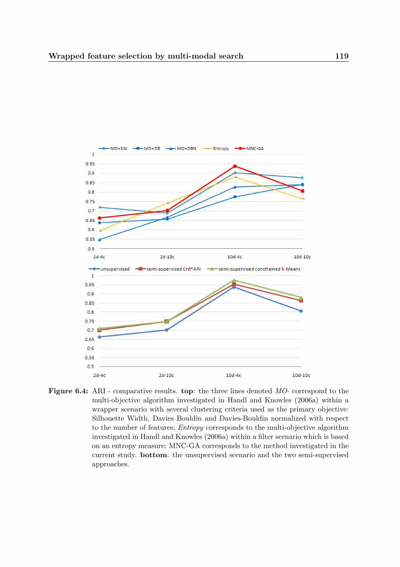
Wrapped feature selection by multi-modal search 119
Figure 6.4: ARI - comparative results. top: the three lines denoted MO- correspond to themulti-objective algorithm investigated in Handl and Knowles (2006a) within awrapper scenario with several clustering criteria used as the primary objective:Silhouette Width, Davies Bouldin and Davies-Bouldin normalized with respectto the number of features; Entropy corresponds to the multi-objective algorithminvestigated in Handl and Knowles (2006a) within a filter scenario which is basedon an entropy measure; MNC-GA corresponds to the method investigated in thecurrent study. bottom: the unsupervised scenario and the two semi-supervisedapproaches.

Wrapped feature selection by multi-modal search 120
algorithm, which is one of the few feasible solutions to unsupervised FS, show that the
multi-modal approach behaves comparable.
Regarding the semi-supervised scenario, the gain in performance is evident compared
to the unsupervised case, especially for the data sets with high numbers of clusters. The
experiments show that constraining the partitions to satisfy the labeled data employing
constrained k-Means generally hastens the retrieval of the relevant features and provides
better results compared to the alternative approach. Additional experiments we have
performed with higher numbers of labeled data items revealed that no significant im-
provements are obtained for the method which incorporates the supervised information
in the fitness function. However, the method which makes use of Constrained k-Means
continues to record performance improvements when increasing the number of labeled
samples because the partitions are guaranteed to satisfy the provided labels.
6.4 Optimized clustering ensembles based on
multi-modal FS
This section proposes unsupervised feature selection as a method to obtain high-quality
partitions in ensemble construction. It can be considered a contribution to two research
directions in unsupervised learning: in ensemble clustering it proposes a new method to
construct both high-quality and diverse clusterings to be used by ensemble methods; in
unsupervised feature selection it proposes a method to deal with the biases inherent due
to the unsupervised nature of the problem.
The current work makes use of the MNC-GA algorithm proposed in section 6.1. As
solution to the dimensionality bias of the unsupervised clustering criteria, we propose
here a new scenario: the solutions of the multi-modal FS algorithm are used to generate
an ensemble of partitions. Then, an ensemble clustering procedure is applied to reach
consensus and to obtain a more accurate partition of the data set. This partition can
be used further to perform FS in a supervised manner; however, this study is beyond
the scope of this work which aims at analyzing the performance of the new ensemble
construction scheme.
The MNC-GA produces optimal partitions in different feature subspaces (conse-
quently with different numbers of clusters), grouped around several optima; the size
of each niche is proportional with the quality of the corresponding partition. We use

Wrapped feature selection by multi-modal search 121
the entire set of partitions obtained at the end of the run of MNC-GA for ensemble
construction. At first glance this seems to be a drawback with regard to diversity. How-
ever, previous studies Domeniconi and Al-Razgan (2009) show that a weighting scheme
which balances the voting mechanism towards the most compact clusters improves con-
siderably the results of ensemble clustering. The MNC-GA algorithm achieves implicitly
such a weighting mechanism through the multiplicity of the partitions obtained.
For each partition in the ensemble, a similarity matrix is computed over the set of data
items, by applying the cosine function on the vectors representing the class assignments
of the data items. The sum over all similarity matrices gives the final similarity matrix
of the data set. The clustering problem reduces then to a graph partitioning problem.
6.4.1 Experiments
The population size in MNC-GA was set to 50. At each iteration the fitness variation
in population is measured and the algorithm is stopped when no significant changes are
recorded during the last 10 iterations, suggesting convergence.
For comparisons with Domeniconi and Al-Razgan (2009), Metis 1 is used to solve the
graph partitioning problem in the final stage of ensemble clustering. Real data sets from
UCI Repository are used; some are modified as in Domeniconi and Al-Razgan (2009)
in order to contain equal-sized classes required by the Metis algorithm. The results are
validated against the known actual partitions and the error rate is computed. Table 1
reports the experimental results as averages and standard deviations over 10 runs.
Problem #items #features(m) # classes(k) k-Means METIS MNC-METIS
Iris 150 4 3 16.46±1.37 16.66 4.33±0.47
LetterAB 1555 16 2 13.16±5.60 10.93 8.04±1.58
satImage 2110 36 2 15.69±0.01 14.83 13.93±1.23
WDBC 424 31 2 20.75±0.00 10.14 9.72±0.42
Table 6.4: Results on real data sets. The average error rate for 10 runs is reported for k-Means and METIS algorithms applied on the original data set and for the ensembleprocedure introduced in this section(MNC-METIS)
1http://glaros.dtc.umn.edu/gkhome/

Wrapped feature selection by multi-modal search 122
6.5 Conclusions
Multi-modal optimization by means of crowding genetic algorithms has been shown to
be a successful scenario in searching for relevant features in clustering. It offers solutions
to the bias induced by the clustering criteria with respect to the cardinality of the feature
subspace and provides high-quality ensembles of partitions.

Chapter 7
A unifying criterion for
unsupervised clustering and feature
selection
Unsupervised feature selection and unsupervised clustering can be successfully ap-
proached as optimization problems by means of global optimization heuristics if an
appropriate objective function is considered. This chapter introduces an objective func-
tion capable of efficiently guiding the search for significant features and simultaneously
for the respective optimal partitions [Breaban and Luchian (2010)]. Experiments con-
ducted on complex synthetic data suggest that the function we propose is unbiased with
respect to both the number of clusters and the number of features.
7.1 Introduction
In view of the definition of clustering, feature selection can be stated as an optimization
problem:
find
w∗ = argmaxwQ(S ′)
where
• w = w1, w2, ...wm ∈ 0, 1m is a binary string;
123

A unifying criterion for unsupervised clustering and feature selection 124
• S ′ is the data set constructed from the original set S and the string w as follows:
S ′ = d′1, d′2, ..., d′n, d′i = w1 · fi1, w2 · fi2, ..., wm · fim,∀i = 1..n;
• Q(S ′) is a function which measures the tendency of data items in set S ′ to group
into well-separated clusters; it can be expressed by means of the entropy (filter
approaches) or of a fitness function which measures the quality of a partition de-
tected by a clustering algorithm (wrapper approaches). In the latter case feature
weighting is akin to solving the clustering problem in different feature spaces.
Our study approaches unsupervised feature selection in a wrapper manner. In this
regard, a new optimization criterion largely unbiased with respect to the number of clus-
ters is introduced in section 7.2. Section 7.3 discusses the normalization of the clustering
criterion with respect to the number of features. Section 7.4 presents a framework for
performing unsupervised feature selection in conjunction with unsupervised clustering
and summarizes the experimental results. Section 7.5 draws conclusions and points to
future work.
7.2 Unsupervised clustering: searching for the
optimal number of clusters
Classical clustering methods, such as k-Means and hierarchical algorithms, are designed
to use prior knowledge on the number of clusters. In k-Means, an iterative process
reallocates data items to the clusters of a k-class partition in order to minimize the
within-cluster variance. Hierarchical clustering adopts a greedy strategy constructing
trees/dendrograms based on the similarity between data items; each level in these den-
drograms corresponds to partitions with a specific number of clusters and the method
offers no guidance regarding the level where the optimal partition is represented (hence,
the optimal number of clusters).
The algorithms mentioned above are local optimizers. In order to design a global
optimizer for the clustering problem, a criterion for ranking all partitions, irrespective of
the number of clusters, is needed. The problem is far for being trivial: with no hint on the
number of clusters, common-sense clustering criteria like minimizing the variance within
clusters and/or maximizing the distance between clusters guide the search towards the
extreme solution - the n-class partition with each class containing exactly one point.

A unifying criterion for unsupervised clustering and feature selection 125
Existing studies in the literature propose and experiment with various clustering
criteria: Bezdek and Pal (1998); Kim and Ramakrishna (2005); Milligan and Cooper
(1985); Raskutti and Leckie (1999). The main concern is the bias these criteria introduce
towards either lower or higher numbers of clusters. Since this bias proved to be hard
to eliminate, multi-objective algorithms were proposed [Handl and Knowles (2005)],
which evaluate the quality of a partition against several criteria. The main drawback
remains the fact that identifying the optimal solution within the final Pareto front is
not straightforward.
The clustering criterion used in the present work originates in the analogy with the
Huygens’ theorem from mechanics, analogy introduced by Diday et al. (1982) and used
further by Luchian (1995). Considering the data set S in the above definitions, the
following notations are used:
W =∑k
i=1
∑d∈Ci δ(ci, d) is the within-cluster inertia computed as the sum of the
distances between all data items d in cluster Ci and their cluster center ci;
B =∑k
i=1 |Ci| · δ(ci, g) is the between-cluster inertia computed as the sum of the
distances between the cluster centers ci and the center of the entire data set g weighted
with the size of each cluster |Ci|.
T =∑n
i=1 δ(di, g) is the total inertia of the data set computed as the sum of the
distances between the data items and the center g of the data set.
In the above center is the gravity center.
The above-mentioned analogy with mechanics can only be applied as an approxima-
tion. The simplest approximation of the Huygens theorem is then
W +B ≈ T (7.1)
According to the above formula, for any partition of the data set, regardless the number
of clusters, the sum W+B is merely constant. Figure 7.1 illustrates this for the case of
a data set with 10 random Gaussian features/variables: W, B, and W+B are computed
for locally optimal partitions of the data set obtained by the k-means algorithm with
the number of clusters varying between 2 and 50.
In view of the Huygens theorem, if the number of clusters is fixed, minimizing W or
maximizing B are equivalent clustering criteria which can be used in general heuristics
[Diday et al. (1982)]. Note that the within-cluster variance is a widely used clustering

A unifying criterion for unsupervised clustering and feature selection 126
Figure 7.1: The within-cluster inertia W, between-cluster inertia B and their sum plottedfor locally optimal partitions obtained with k-means over different numbers ofclusters
criterion in supervised clustering. The Huygens theorem provides an equivalent clus-
tering criterion (namely B), at a lower computational cost, which can be used in a
nearest-neighbor assignment scenario Luchian (1995).
When the number of clusters is unknown both these criteria are useless: they direct
the search towards the extreme n-class partition. However, a corollary of the Huygens
theorem in conjunction with penalties against the increase of the number of clusters
proved to work in unsupervised clustering:(BT
)kis used in Luchian et al. (1994); an
equivalent (in view of the Huygens’ theorem) function(
11+W/B
)kis used in Luchian and
Luchian (1999) in order to use local Mahalanobis distances. Unfortunately, extensive
experiments we conducted recently with these fitness functions, showed that they are
appropriate only for data sets with a small number of features; other penalization factors
may therefore be necessary for higher-dimensional spaces.
Both within-cluster inertia and between-cluster inertia are necessary for a reliable
comparison and evaluation of partitions in different feature subspaces. In this regard,
we minimize the within-cluster inertia and maximize the between-cluster inertia simul-
taneously, through maximizing
F =
(1
1 +W/B
). (7.2)
In order to study the bias this function induces on the number of clusters in unsupervised
clustering, we used the k-Means algorithm to derive partitions for data sets consisting of
between 2 and 20 random Gaussian features. As shown in figure 7.2-left, the function F
is monotonically increasing with respect to the number of clusters, taking smaller values
for higher dimensional data sets. Figure 7.2-right penalizes the increase in the number
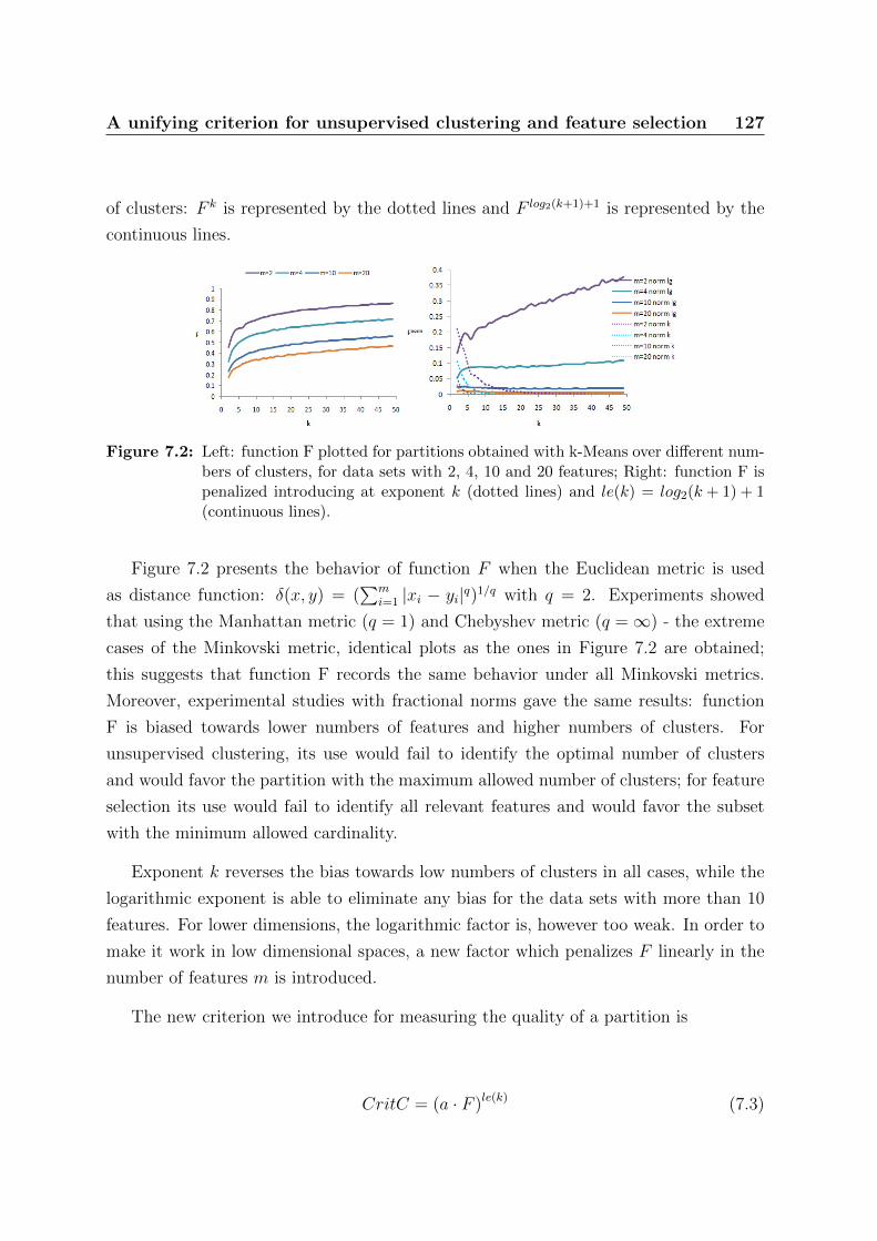
A unifying criterion for unsupervised clustering and feature selection 127
of clusters: F k is represented by the dotted lines and F log2(k+1)+1 is represented by the
continuous lines.
Figure 7.2: Left: function F plotted for partitions obtained with k-Means over different num-bers of clusters, for data sets with 2, 4, 10 and 20 features; Right: function F ispenalized introducing at exponent k (dotted lines) and le(k) = log2(k + 1) + 1(continuous lines).
Figure 7.2 presents the behavior of function F when the Euclidean metric is used
as distance function: δ(x, y) = (∑m
i=1 |xi − yi|q)1/q with q = 2. Experiments showed
that using the Manhattan metric (q = 1) and Chebyshev metric (q =∞) - the extreme
cases of the Minkovski metric, identical plots as the ones in Figure 7.2 are obtained;
this suggests that function F records the same behavior under all Minkovski metrics.
Moreover, experimental studies with fractional norms gave the same results: function
F is biased towards lower numbers of features and higher numbers of clusters. For
unsupervised clustering, its use would fail to identify the optimal number of clusters
and would favor the partition with the maximum allowed number of clusters; for feature
selection its use would fail to identify all relevant features and would favor the subset
with the minimum allowed cardinality.
Exponent k reverses the bias towards low numbers of clusters in all cases, while the
logarithmic exponent is able to eliminate any bias for the data sets with more than 10
features. For lower dimensions, the logarithmic factor is, however too weak. In order to
make it work in low dimensional spaces, a new factor which penalizes F linearly in the
number of features m is introduced.
The new criterion we introduce for measuring the quality of a partition is
CritC = (a · F )le(k) (7.3)

A unifying criterion for unsupervised clustering and feature selection 128
where a = 2·m(2·m+1)
and le(k) = log2(k + 1) + 1 (logarithmic exponent).
CritC takes values in range [0,1] and should be maximized.
This function is studied in the sequel in the context of unsupervised clustering; we test
its capacity of detecting simultaneously the optimal partition and the optimal number
of clusters (see section 4).
7.3 Unsupervised feature selection: searching for
the optimal number of features
Wrapper methods for feature selection evaluate subsets of features based on the qual-
ity of the best partition generated by each subset. In this scenario, an unsupervised
clustering criterion unbiased with respect to the number of clusters and with respect
to the number of features, able to compare different partitions is required in order to
asses the quality of feature subsets. However, existing unsupervised clustering criteria
are not appropriate/fair evaluators in the context of feature subsets of different cardi-
nalities: they are based on computing some distance function for every pair of data
items. Since dimensionality influences the distribution of the distances between data
items, it induces a bias in the objective function with respect to the size of the feature
space. To illustrate this, consider the case of Minkowski distance functions: the mean
of the distribution increases with the size of the feature space because one more feature
introduces one more positive term into the sum; combined with an objective function
which minimizes the between-cluster variance, feature selection will be strongly biased
towards low dimensionality. This example is not unique: it is also the case of the most
popular unsupervised clustering criteria - Davies- Bouldin Index, Sillhouette Width -
which are also biased towards low dimensionality.
The influence of the dimensionality of the data set on distance-based data analy-
sis methods - including clustering techniques, was thoroughly investigated in Aggarwal
et al. (2001). The authors show that in high-dimensional spaces fractional norms are
more appropriate to discriminate between data items. As a consequence, clustering al-
gorithms using fractional norms to measure the distance between data items of large
dimensionality, are more successful. However, fractional norms are not a solution when
a large number of noisy features are present in data.

A unifying criterion for unsupervised clustering and feature selection 129
In the available literature we did not come across an objective function (ranking
criterion) to provide a ranking of partitions with regard to their quality, irrespective
of the number of features. It is the goal of this study to propose a function which, in
the search space defined by all possible subsets of features in conjunction with a variable
number of clusters, assigns a ranking score to each partition that may be defined. The
function we propose may be used by any heuristic searching for the best partition when
both the number of features and the number of clusters vary during the search.
As shown in Figure 7.2, the function CritC (proposed in section 2), monotonically
decreases with the number of features even if factor a penalizes small feature spaces. This
function would point the search towards small feature subsets. In order to eliminate this
bias with respect to the number of features m, we use the factor le(m) = log2(m+1)+1
with the goal of penalizing small values of m. Our new optimization function is:
CritCF = CritC1
le(m) = (a · F )le(k)le(m) (7.4)
Studies we undertook on datasets containing Gaussian features, show that the func-
tion CritCF removes considerably the bias with regard to both the number of clusters
and the number of features, but not completely. Yet, this function is the winner of a
contest with only a few hand-made competitors; a safe assumption would be that better
candidates may exist. We tested this assumption through an automated search process
using Genetic Programming; this search is described in the rest of this section.
Because F is influenced by both the number of features m and the number of clusters
k, we search for a function expressing this dependency. The problem is formulated as fol-
lows: given tuples (m, k, F ), an equation satisfied by them must be determined. We deal
in fact with symbolic regression: the optimization process has to work simultaneously
on the analytical form of the function, the variables involved, and the coefficients.
Using datasets containing only standard Gaussian features, optimal partitions were
constructed with the k-Means algorithm varying the number of clusters k in the range
2-49 and the number of features m in the range 2-20. Then, using formula 7.2 the values
of F were computed for all resulted partitions.
Tuples (m, k, F ), generated in this way, are given as input to a genetic programming
algorithm [Koza (1992)]. The chromosomes are trees which are decoded into functions

A unifying criterion for unsupervised clustering and feature selection 130
over the two variables m and k. The crossover and mutation operators are similar to
those described by Koza. The fitness function computes the ability of each chromosome
to predict the values of F in terms of absolute error of the encoded solution relative
to the input data set. The set of operators is +, -, ·, / ; additionally, the natural
logarithm, the base 2 logarithm and the power function are used.
A chromosome derived from CritCF function was introduced in the initial population
consisting of random generated individuals. CritCF should deliver a constant value for
all the partitions derived in this part of the experiments; however, slight variations exist
and an average denoted by const is computed over all values. Then, F is extracted from
formula 7.3 as shown below and encoded as a GP chromosome.
F =1
a· (const)
le(m)le(k) (7.5)
Several runs of the GP algorithm with different settings were performed, each run
consisting of evaluating about 20 000 new chromosomes derived from the application
of genetic operators. None of the chromosomes generated throughout the run outper-
formed the chromosome encoding formula 7.5. The absolute error obtained by the best
chromosome recorded during the runs of the algorithm was 41% higher compared to the
absolute error recorded by the chromosome encoding formula 7.5.
These first experiments strongly suggest that the function CritCF we propose is a
near-optimal solution; it is largely unbiased with respect to both the number of clusters
and the number of features. It takes values in range [0,1] and should be maximized in
order to simultaneously obtain the best feature subset and partition. This function is
further studied on synthetic complex data sets.
7.4 Experiments
7.4.1 The unsupervised clustering criterion
In order to study the criterion CritC, we undertook comparative studies on complex
synthetic data sets against the most widely used criteria for unsupervised clustering.

A unifying criterion for unsupervised clustering and feature selection 131
The search method
In order to search for the best clustering in a fixed feature space, the K-means algorithm
is run over the given data set with the number of clusters k ranging from 2 to 50. In
order to avoid suboptimal solutions due to unfavorable initialization, K-means is run 10
times and only the best solution with regard to the within-cluster inertia is reported.
This is what we further call one k-Means run.
The data suite
The performance of our clustering criterion CritC in finding the optimal clustering is
evaluated under various scenarios: data sets with lower or higher dimensionality, some
having optimal partitions with a small number of clusters and others having optimal
partitions with a high number of clusters. In this regard the complex benchmark made
available by Julia Handl 1 Handl and Knowles (2005) is used; it represents a standard
cluster model built using multivariate normal distributions. The clusters in a data
set are built iteratively based on covariance matrices which need to be symmetric and
positive definite. Overlapping clusters are rejected and regenerated, until a valid set of
clusters has been found. The covariance matrices are built in such a way to encourage
the production of elongated clusters; this is the reason why k-Means fail to identify in
some test cases the correct partition, as the results in the experimental section show.
Ten data sets of dimensionality d and containing k clusters are created and referred
to as the group of data dd-kc, with d ∈ 2, 10 and k ∈ 4, 10, 20, 40. The size of each
cluster varies uniformly in the range [50,500] for the data sets with 4 and 10 clusters
and in range [10,100] for the data sets with 20 and 40 clusters.
A total of 120 data sets were used in order to study our criterion in the context of
unsupervised clustering.
Validation measures: the Adjusted Rand Index
Each partition returned by k-means is evaluated against the optimal clustering using
the Adjusted Rand Index (ARI) [Hubert (1985)].
1http://dbkgroup.org/handl/generators/

A unifying criterion for unsupervised clustering and feature selection 132
7.4.2 The unsupervised feature selection criterion
Search methods
Wrapper feature selection methods usually involve two distinct heuristics: one for search-
ing the feature space for the optimal feature subset and the other one for searching the
optimal partition, given a feature set. In our approach the latter is performed using
the k-Means algorithm. The former is conducted with two heuristics: a greedy method
named sequential forward selection which is widely used in the context of feature selec-
tion and a global optimization heuristic. Extensive experiments employing two versions
of the greedy algorithm and a multi-modal optimization algorithm provide insight into
the fitness landscape under our criterion.
(A) Sequential forward Selection
Forward selection is a greedy algorithm widely used for feature selection [Dy and
Brodley (2004); Handl and Knowles (2006a); Liu and Motoda (1998)]. In our imple-
mentation it starts with the empty set and iteratively adds the feature which, added to
the already selected features gives the highest value for the CritCF function. For each
candidate feature the k-Means algorithm is run repeatedly with the number of clusters
ranging from 2 to 17 and the best partition is chosen using the CritCF function. The
range of values used for the number of clusters was chosen in order to be consistent with
the genetic algorithm employed in subsection B)as the global search method.
Two versions of this algorithm corresponding to different halting conditions are con-
sidered. In a first scenario, the algorithm is stopped when none of the remaining features
brings any improvement when added to the already selected ones.
A second version of the greedy algorithm is inspired from the experiments described
in Handl and Knowles (2006a) where a fixed number of features are selected and the best
solution is eventually chosen from a Pareto front. As in Handl and Knowles (2006a), the
algorithm selects iteratively up to 20 features which is akin to ranking the most relevant
20 features. The best solution is chosen further based on the fitness values computed
with CritCF for each group of the first i features.
The first algorithm has a reduced time complexity due to the halting condition but
it gets more easily trapped in local optima.

A unifying criterion for unsupervised clustering and feature selection 133
Figure 7.3: Forward Selection 1: Input - the set of all features F ; Output - a subset Scontaining relevant features
bestF itness← 0S ← ∅continue← TRUEwhile continue docontinue← FALSEfor each feature f in F dobestLocalF itness← 0for all nClasses such that 2 ≤ nClasses ≤ 17 do
if (bestLocalF itness < CritCF (kMeans(nClasses, S⋃f))) then
update(bestLocalF itness)end if
end forif (bestF itness < bestLocalF itness) thenbestF itness← bestLocalF itnessfeatureToAdd← fcontinue← TRUE
end ifend forif continue thenS ← S
⋃featureToAdd
F ← F − featureToAddend if
end while

A unifying criterion for unsupervised clustering and feature selection 134
The number of evaluations required by the greedy forward feature selection algorithm
with variable number of clusters is
(kmax − 1) · dmax · d (7.6)
where
• d is the dimensionality of the data set;
• dmax is the maximum cardinality of the feature subsets;
• kmax is the maximum number of clusters allowed while searching for the best par-
tition.
For Handl’s data sets with 100 noisy variables used in this study, the second version of
the greedy algorithm searching for at most 20 relevant features would thus require at
least 32 000 evaluations. The number of evaluations required by the first version of the
algorithm depends on the number of relevant features identified.
(B) A Genetic Algorithm
The Multi-Niche Crowding Genetic Algorithm (MNC GA) presented in section 6.1
of this thesis is used to search for both the optimal feature subset and the respective
optimal number of clusters.
For comparison purposes, many parameter values in our experiments reproduce those
reported in Handl and Knowles (2006a). The maximum number of clusters allowed
during the search is kmax = 17 (only 4 bits encode the number of clusters). The search
space is restricted to solutions with a maximum of dmax = min20, d features from
a total of d features. In addition, in order to speed up the process of identifying the
optimal feature subset, the maximum number of features selected within a chromosome
is gradually increased throughout the run from a maximum of 5 features during the first
generations to 10, then 15 and finally 20 at the end of the run. The risk of getting
trapped in local optima due to this incremental search (specific to greedy algorithms) is
tackled by the crowding GA through maintaining multiple niches in the search space.
The size of the population in MNC-GA is set to pop size = 100 individuals. The
following values give an appropriate balance between exploration/exploitation and a
moderate fitness pressure at replacement: s = 0.10 · pop size, g = 0.15 · pop size,f = 0.10 · pop size.

A unifying criterion for unsupervised clustering and feature selection 135
The most time-consuming part of the algorithm is the evaluation step which mainly
consists of finding the best partition for a given feature set and a given number of clusters.
Each run of the MNC-GA algorithm consisted of 10.000 iterations which correspond to
10.000 evaluations.
At the end of each run of the MNC-GA algorithm a local search was performed
around the best individual in order to avoid sub-optimal numbers of clusters: for the
best feature subset, the k-Means algorithm was run with the number of clusters varying
from k − 2 to k + 2 where k is the number of classes encoded by the best chromosome.
The best partition is chosen to be the one with the best (highest) CritCF value.
The data suite
In order to validate our criterion in the context of unsupervised wrapper feature selection,
a total of 40 data sets were used in this part of the experiments.
Using the multivariate Gaussian cluster model from Section 4.1.3, Handl and Knowles
(2006a) designed small data sets for validating feature selection methods. They created
ten data sets of dimensionality d and containing k clusters, with d ∈ 2, 10 and k ∈2, 4, 10. The size of each cluster is uniformly distributed within the set10,...,50.
Handl and Knowles introduced 100 Gaussian noise variables in each data set in order
to create high-dimensional data, which contain in some cases more dimensions than data
points, a few features being relevant for the classification task. We denote these data
sets by dd-kk-100-gaussian.
We also evaluate the performance of criterion CritCF when other kind of noise than
Gaussian is involved. Therefore, we replaced the Gaussian noisy variables introduced
within the datasets designed by Handl and Knowles with 100 uniform noisy variables
and thus 40 new data sets were created and denoted in the experimental section as
dd-kk-100-uniform.
Tests were also conducted on some real data sets form UCI Repository. The datasets
used represent hand-written digits and letters. The Digits data set has 64 attributes
representing pixels on a 8x8 grid and the Letters data set consist of 16 attributes corre-
sponding to a 4x4 grid. Their values express the intensity of the color.
Since features may be expressed on different scales, all datasets are normalized such
that each feature has mean 0 and standard deviation 1.

A unifying criterion for unsupervised clustering and feature selection 136
Validation measures
Results regarding feature selection can be validated from two perspectives: the quality
of the best found partition reported to the (known) optimal partition, and the quality
of the feature set reported to the (known) relevant features.
The quality of a partition is measured by the Adjusted Rand Index.
The quality of a feature subset is computed with respect to the known relevant
feature set by means of two indexes from information retrieval: precision (equation
6.3) and recall (equation 6.2). Also their combination under harmonic mean known as
F-measure (equation 6.4) is used.
7.4.3 Results
Results for unsupervised clustering
One observation is mandatory for the sake of further discussion: the two criteria CritC
in formula 7.3 and CritCF in formula 7.4 deliver the same ordering on the set of all
partitions in the context of unsupervised clustering in a fixed feature space. Therefore,
the two criteria can be considered as equivalent for the first task investigated in this
chapter which is unsupervised clustering in a fixed feature space; this discussion is
conducted further for the CritCF function.
In order to verify that the clustering criterion does not suffer from any bias with
regard to the number of clusters, tests are made within a larger range. For each data
set, k-Means is run with the number of clusters varying in the range [2, 50].
In case of the data sets dd-kk-100 designed for feature selection, k-Means is run on
the reduced data consisting only of the relevant features. For these test cases, k-Means
is run with the number of clusters varying in range [2, 17], in order to be able to report
these results as upper bounds for feature selection.
Subsequently, the three unsupervised clustering criteria (Davies Bouldin Index, Sil-
houette Width and CritCF) are computed for each of the 49 (respectively 16) partitions
returned by k-Means, in order to select the partition with the optimal number of clus-
ters. The ARI score and the number of clusters k are recorded for the winning partition.

A unifying criterion for unsupervised clustering and feature selection 137
The best partition for each dataset is designated to be the one with the highest ARI
score.
The procedure described above was applied 20 times to each data set. Table 7.1
presents averages and standard deviations over the ARI scores and the numbers of
clusters for best partitions with respect to: 1. the ARI score recorded by k-Means
(Best), 2. Davies-Bouldin Index (DB), 3. Silhouette-Width (SW) and 4. our criterion.
Statistical tests were conducted to verify if the differences of the ARI scores are
significant enough to extract a winner for each type of problem. In this regard, the
3 groups of ARI values corresponding to the 3 clustering criteria, obtained through
repeated independent runs of the algorithm on instances of a given type of problem
(dd-kk) are analyzed. We skip the Kruskal-Wallis test for testing equality of population
medians among the 3 groups because it assumes identically-shaped distributions for all
group. This condition does not hold: the standard deviation is significantly larger in case
of Davies-Bouldin and Silhouette-Width criteria. One reason for the high variance is a
bad performance on one or several test instances. For example, in case of the problem
2d-4c all clustering criteria select partitions with a number of clusters ranging from 3
to 5, except in case of the instance 2d-4c-no5 for which DB and SW criteria select the
partition with only 2 clusters. An opposite example is the problem 10d-4c-100: for
the instance 10d-4c-100-no5 CritCF selects partitions with a number of clusters ranging
from 3 to 5, while SW and mostly DB select partitions with a higher number of clusters,
even up to the maximum allowed value - 17 clusters.
The Wilcoxon Signed-Rank non-parametric test was applied for each problem on the
group of ARI scores determined with CritCF function and the group with the highest
average ARI score among the other two criteria. Where differences are significant (at
the level 1%) the winner is marked in bold.
Table 7.1 shows that the new criterion CritCF achieves the best results in unsuper-
vised clustering in most test cases. In a few cases it is outperformed by the Silhouette
Width Index. However, compared to Silhouette Width Index which has quadratic com-
plexity in the number of data items, CritCF has linear time complexity. The highest
difference in performance between CritCF and the two opponents can be observed in
case of smaller (sparser) data sets dd-4c-100 due to the poor estimation of the number
of clusters by Davies-Bouldin Index and Silhouette Width Index. The high values of
the standard deviation for the number of clusters and, implicitly, for the ARI scores in

A unifying criterion for unsupervised clustering and feature selection 138
Problem Best DB SW CritCF
ARI k ARI k ARI k ARI k
2d-4c 0.9235 4.02 0.8182 3.30 0.8710 3.70 0.8580 4.01
±0.04 ±0.14 ±0.15 ±0.78 ±0.13 ±0.78 ±0.08 ±0.79
2d-10c 0.8359 10.93 0.6869 7.78 0.7800 11.24 0.7945 10.39
±0.07 ±2.09 ±0.14 ±3.35 ±0.10 ±3.37 ±0.08 ±2.44
2d-20c 0.9133 19.63 0.8046 14.17 0.8700 16.71 0.8902 17.45
±0.02 ±2.13 ±0.12 ±3.15 ±0.07 ±2.90 ±0.04 ±2.53
2d-40c 0.8347 39.48 0.7070 25.39 0.8023 34.84 0.7868 30.64
±0.02 ±4.50 ±0.10 ±6.37 ±0.04 ±5.27 ±0.05 ±4.74
10d-4c 0.9711 3.99 0.9158 3.69 0.9044 3.59 0.9327 3.5
±0.02 ±0.07 ±0.14 ±0.64 ±0.14 ±0.66 ±0.04 ±0.50
10d-10c 0.9246 9.21 0.8930 8.62 0.9178 9.03 0.8958 8.36
±0.02 ±0.82 ±0.07 ±1.26 ±0.02 ±0.78 ±0.03 ±1.25
10d-20c 0.9744 20.23 0.9189 17.08 0.9479 18.05 0.9636 20.44
±0.01 ±1.82 ±0.06 ±1.84 ±0.04 ±1.59 ±0.02 ±1.63
10d-40c 0.9582 41.36 0.8849 32.03 0.9282 35.48 0.9459 42.975
±0.01 ±3.25 ±0.05 ±2.89 ±0.03 ±3.12 ±0.02 ±3.23
2d-4c-100 0.8090 3.9 0.6996 3.39 0.6419 2.96 0.7467 4.00
±0.13 ±0.83 ±0.15 ±2.43 ±0.15 ±1.14 ±0.12 ±1.00
2d-10c-100 0.7913 10.7 0.6608 8.44 0.6880 8.945 0.7420 9.65
±0.06 ±2.19 ±0.15 ±4.02 ±0.13 ±4.05 ±0.05 ±2.90
10d-4c-100 0.9610 3.88 0.7963 4.66 0.8600 4.06 0.9263 3.93
±0.05 ±0.32 ±0.26 ±3.52 ±0.22 ±2.53 ±0.12 ±0.44
10d-10c-100 0.8805 9.70 0.8392 8.37 0.8600 9.43 0.8327 8.18
±0.04 ±1.19 ±0.06 ±1.30 ±0.06 ±1.53 ±0.07 ±1.39
Table 7.1: Results on synthetic and real data sets - partitions obtained with the k-Meansalgorithm. The ARI score and the number of clusters k reported here, are com-puted as averages over 20 runs per data set. For each data set, four partitions arereported: the one with the highest ARI value (Best) and the partition found byDavis-Bouldin Index (DB), Silhouette Width (SW) and CritCF function, respec-tively.
case of these latter criteria show that they are more sensitive to minor changes in the
structure of clusters. For a given problem instance, in some experiments these criteria
were able to identify the optimal clustering but in others they showed a bias towards a
higher number of clusters (each experiment consisting of running k-Means with varying

A unifying criterion for unsupervised clustering and feature selection 139
number of clusters). In case of the Silhouette Width index, this sensitivity can be ex-
plained by the fact that it is dependent on each particular assignment (to clusters) of the
data items rather than on cluster representatives. In the case of the k-Means algorithm,
which is highly dependent on the initialization step and yields near-optimal partitions,
this sensitivity is a drawback. CritCF proved to be more robust: in repeated runs on
the same problem instance, it chose partitions with the same number of clusters.
Results for unsupervised wrapper feature selection
Table 7.2 presents the average performance of the genetic algorithm MNC-GA making
use of CritCF as fitness function on the datasets with Gaussian noise: the ARI score
for the best partition obtained in the selected feature space and its number of clusters
k, the size m, the recall and the precision of the selected feature subset. The average
performance over 20 runs of our method is reported for these datasets in order to make
comparisons with the algorithms investigated in Handl and Knowles (2006a). Figure
7.4 shows the comparative results on the performance of CritCF and the algorithms
investigated in Handl and Knowles (2006a) for feature selection:
• the three red lines correspond to the MNC-GA and Forward Selection algorithms
both employing CritCF as evaluation criterion
• the two blue lines correspond to the multi-objective algorithm investigated in Handl
and Knowles (2006a) with Silhouette Width and Davies Bouldin criteria used as
the primary objective;
• the performance of a filter method is represented in yellow. The method was also
investigated in Handl and Knowles (2006a). It returns a Pareto front of solutions
over two objectives: the minimization of an entropy measure and the maximization
of the number of features in order to balance the bias introduced by the first
objective. After the optimal feature subset is extracted the corresponding ARI value
is obtained using k-Means with the optimal number of clusters. This procedure is
quite unfair since the other methods receive no input regarding the number of
clusters.
The gray line corresponds to the best partition that can be obtained using k-Means
with the exact number of clusters, on the optimal standardized feature subset consisting
of the known relevant features. These values provide an upper bound for the methods
under investigation.

A unifying criterion for unsupervised clustering and feature selection 140
All methods implemented in Handl and Knowles (2006a) return a range of solutions
corresponding to different feature cardinalities. The results presented in Handl and
Knowles (2006a) and cited in this chapter are obtained in the following way: for a given
Pareto front, the feature set with the best F-Measure is selected. This procedure requires
supplementary input and thus makes the comparison unfair for the methods which use
the CritCF criterion and work in an entirely unsupervised manner.
Problem ARI k m recall precision F-measure
2d-4c-100-Gaussian 0.5649 6.27 3.85 0.93 0.80 0.86
±0.28 ± 4.77 ± 4.73
2d-10c-100-Gaussian 0.7281 9.52 2 1 1 1
±0.07 ± 3.40 ± 0
10d-4c-100-Gaussian 0.9087 3.95 7.36 0.74 1 0.85
±0.13 ± 0.45 ± 1.33
10d-10c-100-Gaussian 0.8528 8.51 9.20 0.92 1 0.95
±0.07 ± 1.23 ± 0.71
Table 7.2: Results for feature selection obtained with the MNC-GA algorithm using CritCF,on data sets with gaussian noise (100 gaussian features). The ARI score for thebest partition, the number of clusters k, the number of features m, the recall andthe precision of the selected feature space are computed as averages over 20 runson each data set.
Table 7.3 presents the results obtained with the two versions of the Forward Selection
algorithms on the same datasets containing Gaussian noise.
To estimate the real performance of criterion CritCF, an exhaustive search method
should be employed. Because under an exhaustive search the problem becomes in-
tractable, we present in Figure 7.5 the best results (and not averages) obtained by the
genetic algorithm. In this way we obtain a lower bound for the performance of our
criterion if an exhaustive search should be employed. For each problem instance, from
5 runs of MNC-GA on each problem instance, the solution having the highest CritCF
fitness value is retained. For each class of problems (each class consisting of 10 problem
instances) the results are summarized as boxplots over the Adjusted Rand Index. Ex-
periments are performed both for gaussian and uniform noise. For each problem, Figure
7.5 presents the following:

A unifying criterion for unsupervised clustering and feature selection 141
Figure 7.4: Results for the datasets containing Gaussian noise. Adjusted Rand Index (top)and F-Measure (bottom) for the best partition obtained in the feature subspaceextracted with various methods: the three red lines correspond to the MNC-GA and the two versions of Forward selection algorithm using CritCF; the twoblue lines correspond to the multi-objective algorithm investigated in Handl andKnowles (2006a) using Silhouette Widthand Davies Bouldin as the primary ob-jective. The yellow line corresponds to a filter method investigated in Handl andKnowles (2006a) using an entropy measure. The gray line corresponds to the bestpartition that can be obtained with k-Means run on the optimal standardizedfeature subset
• the performance of KMeans over the datasets consisting only of relevant features
and given the correct number of clusters (supervised clustering),
• the performance of KMeans over the datasets consisting only of relevant features
and employing CritCF to determine the correct number of clusters (unsupervised
clustering),
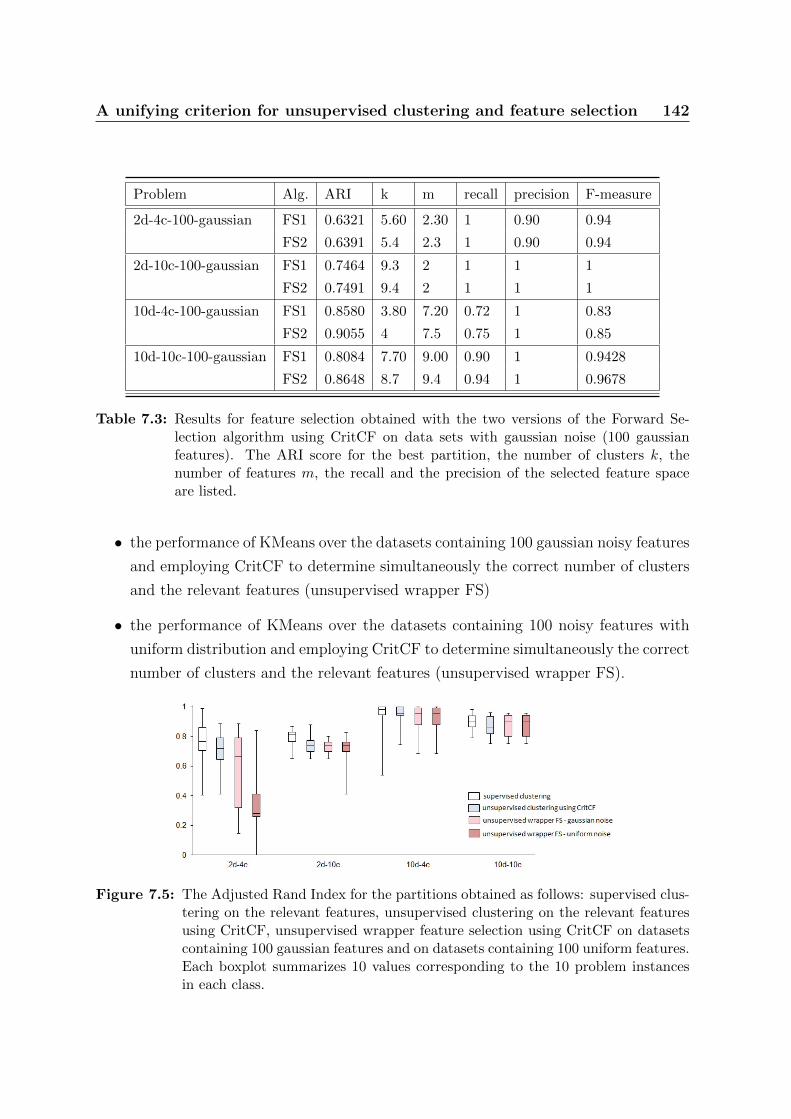
A unifying criterion for unsupervised clustering and feature selection 142
Problem Alg. ARI k m recall precision F-measure
2d-4c-100-gaussian FS1 0.6321 5.60 2.30 1 0.90 0.94
FS2 0.6391 5.4 2.3 1 0.90 0.94
2d-10c-100-gaussian FS1 0.7464 9.3 2 1 1 1
FS2 0.7491 9.4 2 1 1 1
10d-4c-100-gaussian FS1 0.8580 3.80 7.20 0.72 1 0.83
FS2 0.9055 4 7.5 0.75 1 0.85
10d-10c-100-gaussian FS1 0.8084 7.70 9.00 0.90 1 0.9428
FS2 0.8648 8.7 9.4 0.94 1 0.9678
Table 7.3: Results for feature selection obtained with the two versions of the Forward Se-lection algorithm using CritCF on data sets with gaussian noise (100 gaussianfeatures). The ARI score for the best partition, the number of clusters k, thenumber of features m, the recall and the precision of the selected feature spaceare listed.
• the performance of KMeans over the datasets containing 100 gaussian noisy features
and employing CritCF to determine simultaneously the correct number of clusters
and the relevant features (unsupervised wrapper FS)
• the performance of KMeans over the datasets containing 100 noisy features with
uniform distribution and employing CritCF to determine simultaneously the correct
number of clusters and the relevant features (unsupervised wrapper FS).
Figure 7.5: The Adjusted Rand Index for the partitions obtained as follows: supervised clus-tering on the relevant features, unsupervised clustering on the relevant featuresusing CritCF, unsupervised wrapper feature selection using CritCF on datasetscontaining 100 gaussian features and on datasets containing 100 uniform features.Each boxplot summarizes 10 values corresponding to the 10 problem instancesin each class.

A unifying criterion for unsupervised clustering and feature selection 143
Comparing the ARI scores obtained in the original feature space consisting only of
relevant features (Table 7.1) with the ARI scores obtained in the selected normalized
feature space (Table 7.2), a decrease in the computed partition quality can be observed.
Part of this loss can be related to the data normalization performed before feature
selection which, as shown in Duda et al. (2001), can decrease considerably the separa-
bility between clusters making thus more difficult for the algorithm to identify proper
groupings.
In case of the data sets 2d-4c containing gaussian noise, our algorithms using the
criterion CritCF identified the 2 relevant attributes in 7 out of 10 test instances and
delivered partitions with the number of clusters varying between 3 and 5. The poor
average performance reported in Table 7.2 is due to the misleading behavior of our cri-
terion on the remaining 3 test instances. The MNC-GA either selected more features or
chose partitions with a larger number of clusters for these instances. This behavior also
explains the high value of the standard deviation. However, analyzing the chromosomes
in the last generation of the algorithm, we discovered individuals encoding the relevant
features and the right number of clusters; their presence shows that the right configu-
ration constitutes a local optimum in the landscape designed by the CritCF function.
This distorted behavior of our criterion constitutes a drawback for global search meth-
ods; however, the experiments show that it is much reduced in the greedy context: the
two versions of the Forward Selection algorithm added only one irrelevant feature in the
case of these 3 instances determining only on one of them a higher number of clusters
which justifies the high average value for k in Table 7.3.
Regarding the class of problems 2d-10c with gaussian noise, all algorithms selected
the two relevant features for all problem instances as shown by the value of the F-
Measure. The high variance of the number of clusters is due to a higher number of
clusters chosen for two out of ten problem instances. Compared to the results presented
in Table 7.1 for CritCF corresponding to the original relevant feature subset, a loss in
performance is observed because of the normalized features. However, the results are
still better than those obtained with Silhouette Width and Davies-Bouldin criteria in
the original relevant feature space (see Table 7.1).
For the problems with 10 relevant features and gaussian noise, all three algorithms
selected only relevant features but discarded some of them. For the problems with 10
clusters, this seems to be an advantage: the quality of the partitions derived in the
reduced feature space is better, compared to the quality of the partitions derived in the
feature space containing all relevant features (see Table 7.2 vs. Table 7.1).

A unifying criterion for unsupervised clustering and feature selection 144
Even if the F-Measure values in Figure 7.4 bottom corresponding to the criterion
CritCF are lower compared to those reported in Handl and Knowles (2006a), which
were obtained as described above, the ARI scores obtained by our methods are higher
for some problem instances. For example, in case of the problems 10d-4c our methods
obtain the lowest values for the F-measure but outperform most of the algorithms with
regard to the ARI scores. Value 1 for the precision in Tables 7.2 and 7.3 shows that
CritCF manages to remove all the gaussian noisy features. On the other hand, the
recall values show that some relevant features are also discarded. All these observations
suggest the hypotheses that some of the features known to be relevant actually may be
redundant. This hypotheses is suggested as well by experiments reported in Handl and
Knowles (2006a): when the procedure for automated extraction of the optimal solution
from the Pareto front was used, the results concerning F-Measure were significantly
worst while the ARI scores were relatively close.
Unfortunately, analyzing Figure 7.4 no definite winner can be identified: if an algo-
rithm outperforms the others on one class of test instances, there exists an algorithm
which beats it on a different problem. However, when comparing the methods, one must
take into account that the methods based on CritCF function work completely unsu-
pervised while the results reported for the other methods were obtained in a supervised
manner as described above. Moreover, the methods using the function CritCF win with
regard to time-complexity against the other methods presented in the experimental sec-
tion. The first version of the Forward Selection algorithm required an average of 5,000
fitness evaluations for the problem instances with only 2 relevant features and about
17,000 fitness evaluations for the data sets with 10 relevant features. The Multi-Niche
GA was run for only 10,000 fitness evaluations while the second version of the Forward
Selection algorithm and all the methods from Handl and Knowles (2006a) (except the
one based on entropy) employed more than 32,000 fitness evaluations. The quadratic
complexity of the Silhouette Width criterion and the computational effort which must
be payed for post-processing the Pareto front in Handl and Knowles (2006a) must also
be considered.
Regarding the performance of our criterion on datasets with uniform noise, the same
results as for the case of gaussian noise are obtained for the datasets with 10 relevant
features. On the datasets with 2 relevant features and 10 clusters, the algorithm behaved
impeccable on nine out of ten problem instances and selected one irrelevant feature
along with the two relevant features for one problem instance. A significant decrease in
performance can be observed in Figure 7.5 for the class of problems with uniform noise

A unifying criterion for unsupervised clustering and feature selection 145
Problem Alg. ARI k m
Letters AB kMeans 0.7524 2 16
MNC-GA 0.7704 2 8
Digits 56 k-Means 0.9475 2 64
MNC-GA 0.9347 3 6
Table 7.4: Results for feature selection on real data sets. The first line for each data setpresents the performance of k-Means on the initial data set with the correct num-ber of clusters. The second line presents the performance of MNC-GA for unsuper-vised wrapper feature selection: the ARI score, the number of clusters k identifiedand the number of features m selected.
consisting of 2 relevant features and 4 clusters. Only on two problem instances out of
ten in this class, the algorithm selected correctly only the two relevant features. On six
problem instances the algorithm selected the 2 relevant features but also added 1 noisy
features which led to an increasing number of clusters in the selected partition. On the
remaining two problem instances, the algorithm did not identify the relevant features.
However, this class of problem instances seems to be the most difficult one even for the
case of supervised clustering, when k-Means is run on the dataset consisting only of the
relevant features and is supplied with the correct number of clusters; this may be one
reason for the bad performance of the wrapper feature selection method: the clusters
formed in the relevant feature space can not be correctly separated with k-Means, and
the noisy uniform features mislead our criterion towards selecting smaller clusters.
For the Letters and Digits data sets we selected only 2 classes in order to interpret
the results in terms of relevant features: classes A (789 data items) and B (766 data
items) for Letters and classes 5 (376 data items) and 6 (377 data items) for Digits. For
both test cases the MNC-GA was run 5 times each run consisting of 500 iterations; the
best solution under CritCF criterion is reported. The results are presented in Table 7.4.
For the Digits data set the best partition returned with MNC-GA accordingly to CritCF
consisted of 3 clusters with one of the clusters consisting of only 5 data items; a k-Means
run on the selected features with the number of clusters set to 2 returns an ARI score
of 0.9476. The selected features are marked in gray in Figure 7.6.
As shown by the experimental results, CritCF can be used to search for both the most
significant feature subspace and the best partition. The results reported are obtained
on data sets containing more than 90 data items. However, for very small data sets, the

A unifying criterion for unsupervised clustering and feature selection 146
Figure 7.6: Results for MNC-GA on real data. The selected features are marked in gray
between-cluster inertia and within-cluster inertia computed for optimal partitions with
varying number of clusters do not follow the same distribution as the one illustrated in
Figure 7.1, but a more linear one. For this reason, our function was unable to determine
the right number of clusters on most of the test instances in class 2d-2c-100 and 10d-
2c-100. For example, in case of the instances 10d-2c-100-no0 and 10d-2c-100-no8 (which
consist of 118 and respectively 89 data items) CritCF was able to identify the optimum
partition while for the rest of the test instances in the class 10d-2c-100 (which consist
of less than 68 data items) CritCF biased the search process towards higher numbers
of clusters. This phenomenon is common for a wide range of computational problems:
there exist thresholds in the parameter space where certain characteristics of the prob-
lem change dramatically (phase transitions). Therefore, different algorithms may be
appropriate for different instances of the problem. Experiments strongly suggest that
the criterion we propose for unsupervised feature selection and clustering is appropriate
for problem instances (data sets) with more than 70 data items.
7.5 Conclusions
A new clustering criterion was proposed, which is in most cases unbiased with respect
to the number of clusters and which provides at the same time a ranking of partitions
in feature subspaces of different cardinalities. Therefore, this criterion is able to pro-
vide guidance to any heuristic that simultaneously searches for both relevant feature
subspaces and optimal partitions.

Chapter 8
Conclusion and future work
The thesis broke through the main challenges in cluster analysis, by addressing the
following issues:
• dissimilarity measures,
• manifold learning as a preprocessing step prior to clustering,
• algorithms for clustering,
• solution validation,
• feature weighting and selection as methods to improve cluster analysis.
Evolutionary computation techniques applied in clustering were surveyed. New ap-
proaches based on Particle Swarm Optimization and Genetic algorithms were proposed
to tackle some particular clustering problems. Some general-purpose clustering and
feature selection algorithms were designed. An objective function that allows address-
ing unsupervised feature selection and clustering within a unified global optimization
framework was proposed.
As future work, some particular directions with regard to the methods introduced
across the thesis have been already mentioned: i.e. extensions of PSO-kMeans to
the semi-supervised learning scenario, hybridizations between genetic algorithms and
pseudo-boolean programming for the multi-objective graph clustering problem.
A natural path to be followed is to extend wrapper unsupervised feature selection
towards co-clustering in order to identify homogenous groups of objects in different
subspaces of the feature space; the problem is related to local metric learning. An
147

Conclusion and future work 148
important application to be addressed in this context is the analysis of micro-array
data.
Clustering and feature selection are difficult problems with a wide applicability. Evo-
lutionary computation offers powerful optimization techniques. Under these premises, it
is inherent that future studies will successfully approach real-world problems in diverse
domains.


Bibliography
A. Abraham, S. Das, and A. Konar. Document clustering using differential evolution.
In Evolutionary Computation, 2006. CEC 2006. IEEE Congress on, 0 2006.
Ajith Abraham, Swagatam Das, and Sandip Roy. Swarm intelligence algorithms for
data clustering. Soft Computing for Knowledge Discovery and Data Mining, Springer
Verlag, pages 279–313, 2007.
R. L. Ackoff. From data to wisdom. Journal of Applied Systems Analysis, 16:3–9, 1989.
Ada, Wai-Chee Fu, Cheng Chun-Hung, and Cheng Chun-Hung. Entropy-based Subspace
Clustering for Mining Numerical Data. 1999. URL http://citeseerx.ist.psu.edu/
viewdoc/summary?doi=10.1.1.33.1465.
Charu C. Aggarwal, Alexander Hinneburg, and Daniel A. Keim. On the surprising
behavior of distance metrics in high dimensional space. In Lecture Notes in Computer
Science, pages 420–434. Springer, 2001.
Rakesh Agrawal, Johannes Gehrke, Dimitrios Gunopulos, and Prabhakar Raghavan.
Automatic subspace clustering of high dimensional data. Data Min. Knowl. Discov.,
11:5–33, July 2005. ISSN 1384-5810. doi: 10.1007/s10618-005-1396-1. URL http:
//portal.acm.org/citation.cfm?id=1077385.1077386.
Buthainah Al-kazemi and Chilukuri K. Mohan. Multi-phase generalization of the particle
swarm optimization algorithm. In Proceedings of the IEEE Congress on Evolutionary
Computation. IEEE Press, 2002.
Khaled S. Al-Sultana and M. Maroof Khan. Computational experience on four algo-
rithms for the hard clustering problem. Pattern Recogn. Lett., 17:295–308, March
1996. ISSN 0167-8655. doi: http://dx.doi.org/10.1016/0167-8655(95)00122-0. URL
http://dx.doi.org/10.1016/0167-8655(95)00122-0.
150

Bibliography 151
Lenuta Alboaie. Pres - personalized evaluation system in a web community. In IEEE
International Conference on e-Business, pages 64–69, 2008.
Lenuta Alboaie and Tudor Barbu. An automatic user-recognition approach within a
reputation system using a nonlinear hausdorff-derived metric. Numerical Functional
Analysis and Optimization, 29, 2008.
Charles J. Alpert. The ispd98 circuit benchmark suite. In Proc. ACM/IEEE Interna-
tional Symposium on Physical Design, April 98, pages 80–85, 1998.
P. J. Angeline. Using selection to improve particle swarm optimization. In Proceedings
of the IEEE International Conference on Evolutionary Computation, pages 84 – 89.
IEEE Press, 1998. ISBN 0-7803-4869-9.
Mihael Ankerst, Markus M. Breunig, Hans-Peter Kriegel, and J?rg Sander. Optics:
Ordering points to identify the clustering structure. ACM SIGMOD Record, 28(2):
49–60, 1999. ISSN 0163-5808. doi: http://doi.acm.org/10.1145/304181.304187. URL
http://portal.acm.org/citation.cfm?id=304187.
T. Back. Evolutionary Algorithms in Theory and Practice. Oxford University Press,
New York, USA, 1996.
S. De Backer, A. Naud, and P. Scheunders. Non-linear dimensionality reduction tech-
niques for unsupervised feature extraction. Pattern Recognition Letters, 19:711–720,
June 1998. ISSN 0167-8655. doi: http://dx.doi.org/10.1016/S0167-8655(98)00049-X.
URL http://dx.doi.org/10.1016/S0167-8655(98)00049-X.
S. T. Barnardand and H. D. Simon. A fast multilevel implementation of recursive
spectral bisection for partitioning unstructured problems. In Proc. 6ts SIAM Conf.
Parallel Processing for Scientific Computing, pages 711–718, 1993.
Pavel Berkhin. Survey Of Clustering Data Mining Techniques. Technical report, Ac-
crue Software, San Jose, CA, 2002. URL http://citeseerx.ist.psu.edu/viewdoc/
summary?doi=10.1.1.18.3739.
S. Bermejo and J. Cabestany. Large margin nearest neighbor classifiers. In Proceedings
of the 6th International Work-Conference on Artificial and Natural Neural Networks,
page 669676, 2001.
J. C. Bezdek and N. R. Pal. Some new indexes of cluster validity. IEEE Transactions
on Systems, Man, and Cybernetics, 28(3):301–315, 1998.
Bibliography 152
James C. Bezdek. Pattern Recognition with Fuzzy Objective Function Algorithms. Kluwer
Academic Publishers, Norwell, MA, USA, 1981. ISBN 0306406713.
James C. Bezdek, Srinivas Boggavarapu, Lawrence O. Hall, and Amine Bensaid. Genetic
algorithm guided clustering. In International Conference on Evolutionary Computa-
tion, pages 34–39, 1994.
Lon Bottou and Yoshua Bengio. Convergence properties of the k-means algorithms. In
Advances in Neural Information Processing Systems 7, pages 585–592. MIT Press,
1995.
R. Boyd and P. J. Richerson. Culture and the Evolutionary Process. University Of
Chicago Press, 1985.
Mihaela Breaban. Evolving ensembles of feature subsets towards optimal feature se-
lection for unsupervised and semi-supervised clustering. In Proceedings of IEA/AIE,
volume LNAI 6097 of Lecture Notes in Artificial Intelligence, pages 67–76. Springer
Berlin / Heidelberg, 2010a.
Mihaela Breaban. Optimized ensembles for clustering noisy data. In Christian Blum
and Roberto Battiti, editors, Learning and Intelligent Optimization, volume 6073 of
Lecture Notes in Computer Science, pages 220–223. Springer Berlin / Heidelberg,
2010b.
Mihaela Breaban and Henri Luchian. Pso under an adaptive scheme. In Proceedings
of the IEEE Congress on Evolutionary Computation, pages 1212–1217. IEEE Press,
2005.
Mihaela Breaban and Henri Luchian. Feature weighting with multi-niche genetic algo-
rithms. In Proceedings of the 10th Genetic and Evolutionary Computation Conference.
ACM, July 2009.
Mihaela Breaban and Henri Luchian. A unifying criterion for unsuper-
vised clustering and feature selection. Pattern Recognition, In Press, Cor-
rected Proof:–, 2010. ISSN 0031-3203. doi: DOI:10.1016/j.patcog.2010.10.
006. URL http://www.sciencedirect.com/science/article/B6V14-51858T4-1/
2/95eefca58562a45238dd50731f51eb13.
Mihaela Breaban and Silvia Luchian. Shaping up clusters with pso. In Proceedings
of the 2008 10th International Symposium on Symbolic and Numeric Algorithms for
Scientific Computing, pages 532–537, Washington, DC, USA, 2008. IEEE Computer

Bibliography 153
Society. ISBN 978-0-7695-3523-4. doi: 10.1109/SYNASC.2008.70.
Mihaela Breaban, Henri Luchian, and Dan Simovici. Genetic-entropic clustering. In
11eme Confrence Internationale Francophone sur l’Extraction et la Gestion des Con-
naissances EGC 2011, (in press).
Mihaela Breaban, Madalina Ionita, and Cornelius Croitoru. A pso approach to constraint
satisfaction. In Proceedings of the IEEE Congress on Evolutionary Computation, pages
1948–1954. IEEE Press, 2007.
Mihaela Breaban, Lenuta Alboaie, and Henri Luchian. Guiding users within trust net-
works using swarm algorithms. In Proceedings of the Eleventh conference on Congress
on Evolutionary Computation, CEC’09, pages 1770–1777, Piscataway, NJ, USA, 2009.
IEEE Press. ISBN 978-1-4244-2958-5.
H. J. Bremermann. The evolution of intelligence. the nervous system as a model of
its environment. Technical Report No.1, Department of Mathematics, University of
Washington, Seattle.
Richard Butterworth, Gregory Piatetsky-Shapiro, and Dan A. Simovici. On feature
selection through clustering. In ICDM, pages 581–584, 2005.
Duo Chen, Du-Wu Cui, and Chao-Xue Wang. Weighted fuzzy c-means clustering based
on double coding genetic algorithm. Lecture Notes in Computer Science, Intelligent
Computing, 4113/2006:622–633, 2006.
Aaron Clauset, M. E. J. Newman, and Cristopher Moore. Finding community structure
in very large networks. Physical Review, 2004.
M. Clerc. The swarm and the queen: towards a deterministic and adaptive particle
swarm optimization. In Proceedings of the IEEE Congress on Evolutionary Com-
putation, volume 3, pages 1951–1957, 1999. doi: 10.1109/CEC.1999.785513. URL
http://dx.doi.org/10.1109/CEC.1999.785513.
C.A.C. Coello and M.S. Lechunga. Mopso: A proposal for multiple objective particle
swarm optimization. In Proceedings of the IEEE Congress on Evolutionary Computa-
tion, pages 1051–1056. IEEE Press, 2002.
D. W. Corne, N. R. Jerram, J. D. Knowles, and M. J. Oates. Apesa-ii: regionbased selec-
tion in evolutionary multiobjective optimization. In Proc. Genetic and Evolutionary
Computation Conference, pages 283–290, 2001.

Bibliography 154
Xiaohui Cui, Thomas E. Potok, and Paul Palathingal. Document clustering using parti-
cle swarm optimization. In IEEE Swarm Intelligence Symposium, The Westin, 2005.
David L. Davies and Donald W Bouldin. A cluster separation measure. IEEE Transac-
tions on Pattern Analysis and Machine Intelligence, 1(2):224–227, 1979.
Kenneth Alan De Jong. An analysis of the behavior of a class of genetic adaptive systems.
PhD thesis, Ann Arbor, MI, USA, 1975. AAI7609381.
Kalyanmoy Deb and David E. Goldberg. An investigation of niche and species formation
in genetic function optimization. In Proceedings of the 3rd International Conference on
Genetic Algorithms, pages 42–50, San Francisco, CA, USA, 1989. Morgan Kaufmann
Publishers Inc. ISBN 1-55860-066-3. URL http://portal.acm.org/citation.cfm?
id=645512.657099.
D. Defays. An efficient algorithm for a complete link method. Comput. J., 20(4):364–366,
1977.
A. P. Dempster, N. M. Laird, and D. B. Rubin. Maximum Likelihood from Incom-
plete Data via the EM Algorithm. Journal of the Royal Statistical Society. Series B
(Methodological), 39(1):1–38, 1977. ISSN 00359246.
Inderjit S. Dhillon and Dharmendra S. Modha. A data-clustering algorithm on dis-
tributed memory multiprocessors. In Large-Scale Parallel Data Mining, pages 245–
260, 1999.
Inderjit S. Dhillon, Subramanyam Mallela, and Rahul Kumar. Enhanced word cluster-
ing for hierarchical text classification. In Proceedings of the eighth ACM SIGKDD
international conference on Knowledge discovery and data mining, KDD ’02, pages
191–200, New York, NY, USA, 2002. ACM. ISBN 1-58113-567-X. doi: http://doi.acm.
org/10.1145/775047.775076. URL http://doi.acm.org/10.1145/775047.775076.
E. Diday, J. Lemaire, J. POuget, and F. Testu. Elements d’analyse de donnees. Dunod,
1982.
Chris Ding and Xiaofeng He. K-means clustering via principal component analysis. In
Proceedings of the twenty-first international conference on Machine learning, ICML
’04, pages 29–, New York, NY, USA, 2004. ACM. ISBN 1-58113-828-5. doi: http://doi.
acm.org/10.1145/1015330.1015408. URL http://doi.acm.org/10.1145/1015330.
1015408.

Bibliography 155
C. Domeniconi and M. Al-Razgan. Weighted cluster ensembles: Methods and analysis.
ACM Transactions on Knowledge Discovery from Data, 2, 2009.
C. Domeniconi and D. Gunopulos. Adaptive nearest neighbor classification using support
vector machines. IEEE Transactions on Pattern Analysis and Machine Intelligence,
24:1281 – 1285, 2002.
Marco Dorigo and Thomas Stutzle. Ant Colony Optimization. Bradford Company,
Scituate, MA, USA, 2004. ISBN 0262042193.
Richard O. Duda, Peter E. Hart, and David G. Stork. Pattern classification. Wiley, 2
edition, November 2001. ISBN 0471056693. URL http://www.worldcat.org/isbn/
0471056693.
Fridlyand J. Dudoit, S. Bagging to improve the accuracy of a clustering procedure.
Bioinformatics, 9:10901099, 2003.
D. Dumitrescu. Genetic chromodynamics. Studia Universitatis Babes-Bolyai Cluj-
Napoca, Ser. Informatica, 45:39–50, 2000.
D. Dumitrescu and Kroly Simon. Evolutionary prototype selection. In Proceedings of the
International Conference on Theory and Applications of Mathematics and Informatics
ICTAMI, pages 183–190, 2003.
D. Dumitrescu, B. Lazzerini, and L.C. Jain. Fuzzy sets and their application to clustering
and training. CRC Press, Inc., Boca Raton, FL, USA, 2000.
J. C. Dunn. A Fuzzy Relative of the ISODATA Process and Its Use in Detecting
Compact Well-Separated Clusters. Journal of Cybernetics, 3(3):32–57, 1973. doi: 10.
1080/01969727308546046. URL http://dx.doi.org/10.1080/01969727308546046.
J. C. Dunn. Well separated clusters and optimal fuzzy-partitions. Journal of Cybernetics,
4:95–104, 1974.
Jennifer Dy and Carla Brodley. Feature selection for unsupervised learning. Journal of
Machine Learning Research, 5:845–889, 2004.
Martin Ester, Hans-Peter Kriegel, Jrg Sander, and Xiaowei Xu. A density-based algo-
rithm for discovering clusters in large spatial databases with noise. In Proc. of 2nd
International Conference on Knowledge Discovery and, pages 226–231, 1996.
Bibliography 156
Per-Olof Fjllstrm. Algorithms for graph partitioning: A survey. Linkping Electronic
Articles in Computer and Information Science, 3, 1998.
L. J. Fogel, A. J. Owens, and M. J. Walsh. Artifficial Intelligence through Simulated
Evolution. John Wiley, New York, USA, 1966.
E. Forgy. Cluster analysis of multivariate data: Efficiency versus interpretability of
classification. Biometrics, 21(3):768–769, 1965.
Chris Fraley and Adrian E. Raftery. Model-based clustering, discriminant analysis and
density estimation. Journal of the American Statistical Association, 97:611–631, 2002.
Alex S. Fraser. Simulations of genetic systems by automatic digital computers. Austral.
J. Biol. Sci., 10.
A. Fred and A.K. Jain. Combining multiple clustering using evidence accumulation.
IEEE Trans. Pattern Analysis and Machine Intelligence, 6:835850, 2005.
Guojun Gan, Ma Chaoqun, and Wu Jianhong. Data Clustering: Theory, Algorithms,
and Application. ASA-SIAM Series on Statistics and Applied Probability, 2007.
P. Ganarski, Alexandre Blansche, and A. Wania. Comparison between two coevolution-
ary feature weighting algorithms in clustering. Pattern Recognition, 41(3):983–994,
March 2008.
Joydeep Ghosh and Alexander Strehl. Similarity-based text clustering: A comparative
study. In Grouping Multidimensional Data, Recent Advances in Clustering.
M. Girvan and M. E. J. Newman. Community structure in social and biological networks.
In Proceedings of the National Academy of Sciences USA, pages 7821–7826, 2002.
A. Gog, D. Dumitrescu, and B. Hirsbrunner. Community detection in complex networks
using collaborative evolutionary algorithms. Lecture Notes in Computer Science, Ad-
vances in Artificial Life, 2007.
Jennifer Golbeck. Computing and Applying Trust in Web-based Social Networks. PhD
thesis, University of Maryland, 2005.
S. Guha. Cure: an efficient clustering algorithm for large databases. Information Sys-
tems, 26(1):35–58, March 2001. ISSN 03064379. doi: 10.1016/S0306-4379(01)00008-4.
URL http://dx.doi.org/10.1016/S0306-4379(01)00008-4.
Bibliography 157
Isabelle Guyon and Andre Elisseeff. An introduction to variable and feature selection.
Journal of Machine Learning Research, 3:1157–1182, March 2003. ISSN 1532-4435.
S. T. Hadjitodorov, L. I. Kuncheva, and L.P. Todorova. Moderate diversity for better
cluster ensembles. Information Fusion, 7:264–275, 2006.
L. O. Hall, B. Ozyurt, and J. C. Bezdek. Clustering with a genetically optimized ap-
proach. IEEE Transactions on Evolutionary Computation, 3:103–112, 1999.
Julia Handl and Joshua Knowles. Improving the scalability of multiobjective clustering.
In Proceedings of the Congress on Evolutionary Computation, pages 2372–2379. IEEE
Press, 2005.
Julia Handl and Joshua Knowles. Feature subset selection in unsupervised learning
via multiobjective optimization. International Journal of Computational Intelligence
Research, 2(3):217–238, 2006a.
Julia Handl and Joshua Knowles. Semi-supervised feature selection via multiobjective
optimization. In Proceedings of the International Joint Conference on Neural Net-
works, pages 3319–3326, 2006b.
Julia Handl, Joshua Knowles, and Marco Dorigo. Ant-based clustering and topographic
mapping. Artificial Life, 12, 2005.
T. Hastie and R. Tibshirani. Discriminant adaptive nearest neighbor classification. IEEE
Pattern Analysis and Machine Intelligence, 18:607–616, 1996.
J.H. Holland. Adaptation in Natural and Artificial Systems: An Introductory Analysis
with Applications to biology, control and artificial intelligence. 1998.
Yi Hong, Sam Kwong, Yuchou Chang, and Qingsheng Ren. Consensus unsupervised
feature ranking from multiple views. Pattern Recognition Letters, 29:595–602, 2008.
T. Hu, W. Zao, X. Wang, and Z. Li. A comparison of three graph partitioning based
methods for consensus clustering. Rough Sets and Knowledge Technology, LNAI 4062,
page 468475, 2006.
X. Hu and R. C. Eberhart. Tracking dynamic systems with pso: where’s the cheese? In
Proceedings of the workshop on particle swarm optimization, pages 80–83, 2001.
X. Hu and R. C. Eberhart. Multiobjective optimization using dynamic neighborhood
particle swarm optimization. In Proceedings of the IEEE Congress on Evolutionary

Bibliography 158
Computation, pages 1677–1681. IEEE Press, 2002a.
X. Hu and R. C. Eberhart. Solving constrained nonlinear optimization problems with
particle swarm optimization. In Proceedings of the Sixth World Multiconference on
Systemics, Cybernetics and Informatics, 2002b.
X. Hu, R. C. Eberhart, and Y. Shi. Swarm intelligence for permutation optimization:
a case study on n-queens problem. In Proceedings of the IEEE Swarm Intelligence
Symposium, pages 243–246. IEEE Press, 2003.
A. Hubert. Comparing partitions. Journal of Classification, 2:193–198, 1985.
Madalina Ionita, Mihaela Breaban, and Cornelius Croitoru. A new scheme of using
inference inside evolutionary computation techniques to solve csps. In Proc. of 8th
International Symposium on Symbolic and Numeric Algorithms for Scientific Com-
puting, Natural Computing and Applications Workshop, pages 323–329. IEEE Press,
2006a.
Madalina Ionita, Cornelius Croitoru, and Mihaela Breaban. Incorporating inference
into evolutionary algorithms for max-csp. In 3rd International Workshop on Hybrid
Metaheuristics, LNCS 4030, pages 139–149. Springer-Verlag, 2006b.
Madalina Ionita, Mihaela Breaban, and Cornelius Croitoru. Evolutionary computation
in constraint satisfaction. New Achievements in Evolutionary Computation, INTECH
Vienna, 2010.
A. K. Jain and A. Fred. Data clustering using evidence accumulation. In In Proc. 16th
International Conference on Pattern Recognition(ICPR02), page 276280, 2002.
A. K. Jain, M. N. Murty, and P. J. Flynn. Data clustering: a review. ACM Comput.
Surv., 31(3):264–323, September 1999. ISSN 0360-0300.
D. R. Jones and M. A. Beltramo. Solving partitioning problems with genetic algorithms.
In 4th International Conference on Genetic Algorithms, pages 442–45O, 1991.
Kenneth A. De Jong. Evolutionary Computation. A Unified Approach. MIT Press, 2006.
Sepandar D. Kamvar, Dan Klein, and Christopher D. Manning. Interpreting and extend-
ing classical agglomerative clustering algorithms using a model-based approach. In
Proceedings of the Nineteenth International Conference on Machine Learning, ICML
’02, pages 283–290, San Francisco, CA, USA, 2002. Morgan Kaufmann Publishers
Inc. ISBN 1-55860-873-7. URL http://portal.acm.org/citation.cfm?id=645531.

Bibliography 159
656166.
George Karypis and Vipin Kumar. A fast and high quality multilevel scheme for parti-
tioning irregular graphs. SIAM Journal on Scientific Computing, 20:359–392, 1998.
George Karypis, Eui-Hong (Sam) Han, and Vipin Kumar. Chameleon: Hierarchical
clustering using dynamic modeling. Computer, 32:68–75, 1999. ISSN 0018-9162. doi:
http://doi.ieeecomputersociety.org/10.1109/2.781637.
Leonard Kaufman and Peter J. Rousseeuw. Finding Groups in Data: An Introduction
to Cluster Analysis (Wiley Series in Probability and Statistics). Wiley-Interscience,
2005. ISBN 0471735787. URL http://www.worldcat.org/isbn/0471735787.
J. Kennedy. Small worlds and mega-minds: Effects of neighborhood topology on particle
swarm performance. In Proceedings of the IEEE Congress of Evolutionary Computa-
tion, volume 3, pages 931–1938. IEEE Press, 1999. doi: 10.1109/CEC.1999.785513.
J. Kennedy and R.C. Eberhart. Particle swarm optimization. In Proceedings of the 1995
IEEE International Conference on Neural Networks, volume 4, pages 1942–1948. IEEE
Press, 1995.
J. Kennedy and R.C. Eberhart. A discrete binary version of the particle swarm algo-
rithm. In Proceedings of the World Multiconference on Systemics, Cybernetics and
Informatics, pages 4104–4109, 1997.
James Kennedy. Population structure and particle swarm performance. In In: Pro-
ceedings of the Congress on Evolutionary Computation (CEC 2002, pages 1671–1676.
IEEE Press, 2002.
James Kennedy and Rui Mendes. R.: Neighborhood topologies in fully-informed and
best-ofneighborhood particle swarms. In In: Proceedings of the 2003 IEEE SMC
Workshop on Soft Computing in Industrial Applications (SMCia03, pages 45–50. IEEE
Computer Society, 2003.
B. W. Kernighan and S. Lin. An efficient heuristic procedure for partitioning graphs.
The Bell system technical journal, 49(1):291–307, 1970.
Minho Kim and R. S. Ramakrishna. Some new indexes of cluster validity. Pattern
Recognition Letters, 26(15):2353–2363, 2005.
Y. Kim, W. N. Street, and F. Menczer. Evolutionary model selection in unsupervised
learning. Intelligent Data Analysis, 6(6):531–556, 2002.

Bibliography 160
Raymond W. Klein and Richard C. Dubes. Experiments in projection and clustering by
simulated annealing. Pattern Recognition, 22(2):213 – 220, 1989. ISSN 0031-3203.
J. Kleinberg. An impossibility theorem for clustering. In S. Becker, S. Thrun, and
K. Obermayer, editors, Advances in Neural Information Processing Systems, pages
446–453. MIT Press, 2002. ISBN 0-262-02550-7. URL http://citeseer.ist.psu.
edu/kleinberg02impossibility.html.
Teuvo Kohonen. Self-organizing maps. Springer-Verlag New York, Inc., Secaucus, NJ,
USA, 1997. ISBN 3-540-62017-6.
Jan Komorowski, Zdzislaw Pawlak, Lech Polkowski, and Andrzej Skowron. Rough sets:
A tutorial. 1998.
Abdullah Konak, David W. Coit, and Alice E. Smith. Multi-objective optimization using
genetic algorithms: A tutorial. Reliability Engineering & System Safety, 91(9):992–
1007, September 2006. URL http://www.sciencedirect.com/science/article/
B6V4T-4J0NY2F-2/2/97db869c46fc43f457f3d509adaa15b5.
John Koza. Genetic Programming: On the Programming of Computers by Means of
Natural Selection. MIT Press, Cambridge, MA, 1992.
T. Krink, J. S. Vesterstrom, and J. Riget. Particle swarm optimisation with spa-
tial particle extension. In Proceedings of the Evolutionary Computation on 2002.
CEC ’02. Proceedings of the 2002 Congress - Volume 02, CEC ’02, pages 1474–1479,
Washington, DC, USA, 2002. IEEE Computer Society. ISBN 0-7803-7282-4. URL
http://portal.acm.org/citation.cfm?id=1251972.1252447.
K. Krishna and M. Narasimha Murty. Genetic k-means algorithm. Systems, Man, and
Cybernetics, Part B: Cybernetics, IEEE Transactions on, 29(3):433 –439, June 1999.
ISSN 1083-4419. doi: 10.1109/3477.764879.
Ravindra Krovi. Genetic algorithms for. clustering: A preliminary investigation. In
Proceedings of the Twenty-Fifth Hawaii International Conference on System Sciences,
pages 540–544. IEEE Computer Society Press, 1991.
E.C. Laskari and M.N. Vrahatis K.E. Parsopoulos. Particle swarm optimization for inte-
ger programming. In Proceedings of the IEEE Congress on Evolutionary Computation,
pages 1582–1587. IEEE Press, 2002.

Bibliography 161
Huan Liu and Hiroshi Motoda. Feature Selection for Knowledge Discovery and Data
Mining. Kluwer Academic Publishers, Norwell, MA, USA, 1998.
L.Talavera. Feature selection as a preprocessing step for hierarchical clustering. In
Proceedings of the Sixteenth International Conference on Machine Learning, pages
389–398. Morgan Kaufmann, San Francisco, CA, 1990.
S. Luchian. An evolutionary approach to unsupervised automated classification. In Pro-
ceedings of EUFIT’95 - European Forum of Intelligent Techniques. ELITE (European
Laboratory for Intelligent Techniques) and Verlag Mainz, 1995.
S. Luchian and H. Luchian. Three evolutionary approaches to classification problems.
In Evolutionary Algorithms in Computer Science, pages 351–380. John Wiley & Sons,
Chichester-New York-Toronto, 1999.
Silvia Luchian, Henri Luchian, and Mihai Petriuc. Evolutionary automated classification.
In Proceedings of 1st Congress on Evolutionary Computation, pages 585–588, 1994.
Morten Lvbjerg, Thomas Kiel Rasmussen, and Thiemo Krink. Hybrid particle swarm
optimiser with breeding and subpopulations. In Proceedings of the Genetic and Evolu-
tionary Computation Conference (GECCO-2001, pages 469–476. Morgan Kaufmann,
2001.
Paolo Massa and Paolo Avesani. Trust metrics on controversial users: balancing between
tyranny of the majority and echo chambers. International Journal on Semantic Web
and Information Systems (IJSWIS), 2007.
Ujjwal Maulik and Sanghamitra Bandyopadhyay. Genetic algorithm-based clustering
technique. Pattern Recognition, 33(9):1455 – 1465, 2000. ISSN 0031-3203.
G.W. Milligan and M. CJ Cooper. An examination of procedures for determining the
number of clusters in a data set. Psychometrika, 50:159–179, 1985.
Dharmendra S. Modha and W. Scott Spangler. Feature weighting in k-means clustering.
Machine Learning, 52(3):217–237.
M. Morita, R. Sabourin, F. Bortolozzi, and C. Y. Suen. Unsupervised feature selection
using multi-objective genetic algorithms for handwritten word recognition. In Proceed-
ings of the Seventh International Conference on Document Analysis and Recognition,
pages 666–671. IEEE Press, New York, 2003.

Bibliography 162
Olfa Nasraoui, Elizabeth Leon, and Raghu Krishnapuram. Unsupervised niche cluster-
ing: Discovering an unknown number of clusters in noisy data sets. In Ashish Ghosh
and Lakhmi Jain, editors, Evolutionary Computation in Data Mining, volume 163 of
Studies in Fuzziness and Soft Computing, pages 157–188. Springer Berlin / Heidelberg,
2005.
H. Pan, J. Zhu, and D. Han. Genetic algorithms applied to multi-class clustering for
gene expression data. Genomics Proteomics Bioinformatics, 1(4):279–287, November
2003. ISSN 1672-0229.
Zdzislaw Pawlak. Rough sets (abstract). In Proceedings of the 1995 ACM 23rd annual
conference on Computer science, CSC ’95, pages 262–264, New York, NY, USA, 1995.
ACM. ISBN 0-89791-737-5. doi: http://doi.acm.org/10.1145/259526.277421. URL
http://doi.acm.org/10.1145/259526.277421.
Karl Pearson. On lines and planes of closest fit to systems of points in space. Philosoph-
ical Magazine, 2(6):559–572, 1901.
Dan Pelleg and Andrew Moore. X-means: Extending K-means with efficient estima-
tion of the number of clusters. In In Proceedings of the 17th International Conf.
on Machine Learning, pages 727–734, 2000. URL http://citeseerx.ist.psu.edu/
viewdoc/summary?doi=10.1.1.19.3377.
Sang-Ho Prak, Ju-Hong Lee, and Deok-Hwan Kim. Spatial clustering based on moving
distance in the presence of obstacles. Lecture Notes in Computer Science: Advances
in Databases: Concepts, Systems and Applications, 4443:1024–1027, 2007.
Gregorio Toscano Pulido and Carlos A. Coello Coello. A constraint-handling mechanism
for particle swarm optimization. In Proceedings of the 2004 Congess on Evolutionary
Computation, pages 1396–1403. IEEE Press, 2004.
Nicholas J. Radcliffe, Patrick D. Surry, Eh Jz, and Eh Jz. Fitness variance of formae
and performance prediction. Foundations of Genetic Algorithms, pages 51–72, 1995.
Gunther R. Raidl and Jens Gottlieb. Empirical analysis of locality, heritability and
heuristic bias in evolutionary algorithms: A case study for the multidimensional knap-
sack problem. Evolutionary Computation, 13(4):441–475, 2005.
Bhavani Raskutti and Christopher Leckie. An evaluation of criteria for measuring the
quality of clusters. In Proceedings of the 16th international joint conference on Ar-
tificial intelligence - Volume 2, pages 905–910, San Francisco, CA, USA, 1999. Mor-

Bibliography 163
gan Kaufmann Publishers Inc. URL http://portal.acm.org/citation.cfm?id=
1624312.1624348.
Ingo Rechenberg. Evolutionstrategie: Optimierung Technisher Systeme nach Prinzipien
der Biologischen Evolution. Frommann-Holzboog Verlag, Stuttgart, 1973.
Jiangtao Ren, Zhengyuan Qiu, Wei Fan, Hong Cheng, and Philip S. Yu. Forward semi-
supervised feature selection. In Advances in Knowledge Discovery and Data Mining
(LNCS), pages 970–976, May 2008.
J. Riget and J. Vesterstroem. A diversity-guided particle swarm optimizer - the ARPSO.
2002. URL http://citeseerx.ist.psu.edu/viewdoc/summary?doi=10.1.1.19.
2929.
P. J. Rousseeuw. Silhouettes: a graphical aid to the interpretation and validation of
cluster analysis. Journal of Computational and Applied Mathematics, 20(1):53–65,
1987.
J. W. Sammon. A nonlinear mapping for data structure analysis. IEEE Trans. Comput.,
18:401–409, May 1969. ISSN 0018-9340. doi: 10.1109/T-C.1969.222678. URL http:
//portal.acm.org/citation.cfm?id=1310162.1310727.
I. Sarafis, A. M. S. Zalzala, and P. W. Trinder. A genetic rule-based data cluster-
ing toolkit. In Proceedings of the Evolutionary Computation on 2002. CEC ’02.
Proceedings of the 2002 Congress - Volume 02, CEC ’02, pages 1238–1243, Wash-
ington, DC, USA, 2002. IEEE Computer Society. ISBN 0-7803-7282-4. URL
http://portal.acm.org/citation.cfm?id=1251972.1252396.
Satu Elisa Schaeffer. Graph clustering. Computer Science Review, Elsevier, I:27–64,
2007.
Bernhard Scholkopf, Alexander Smola, and Klaus-Robert Muller. Nonlinear component
analysis as a kernel eigenvalue problem. Neural Comput., 10:1299–1319, July 1998.
ISSN 0899-7667. doi: 10.1162/089976698300017467. URL http://portal.acm.org/
citation.cfm?id=295919.295960.
Shokri Z. Selim and K. Alsultan. A simulated annealing algorithm for the cluster-
ing problem. Pattern Recognition, 24(10):1003 – 1008, 1991. ISSN 0031-3203.
doi: DOI:10.1016/0031-3203(91)90097-O. URL http://www.sciencedirect.com/
science/article/B6V14-48MPMB9-132/2/b922f1f481a26f67f4338ea07e3861d0.

Bibliography 164
Yuhui Shi and Russell C. Eberhart. Parameter selection in particle swarm optimization.
In EP ’98: Proceedings of the 7th International Conference on Evolutionary Program-
ming VII, pages 591–600, London, UK, 1998. Springer-Verlag. ISBN 3540648917.
URL http://portal.acm.org/citation.cfm?id=647902.738978.
R. Sibson. Slink: An optimally efficient algorithm for the single-link cluster method.
Computer Journal, 16(1):30–34, 1973.
Horst D. Simon. Partitioning of unstructured problems for parallel processing, 1991.
D. A. Simovici and C. Djeraba. Mathematical Tools for Data Mining – Set Theory,
Partial Orders, Combinatorics. Springer-Verlag, London, 2008.
Dan A. Simovici, Dana Cristofor, and Laurentiu Cristofor. Impurity measures in
databases. Acta Inf., 38(5):307–324, 2002.
Nicolaj Sndberg-madsen, Casper Thomsen, and Jose M. Pena. Unsupervised feature
subset selection. In Proceedings of the Workshop on Probabilistic Graphical Models
for Classification (within ECML 2003), 2003.
M. Steinbach, G. Karypis, and V. Kumar. A comparison of document clustering tech-
niques, 2000. URL http://citeseerx.ist.psu.edu/viewdoc/summary?doi=10.1.
1.34.1505.
R. Storn and K. Price. Differential Evolution: A Simple and Efficient Heuristic for
global Optimization over Continuous Spaces. Journal of Global Optimization, 11(4):
341–359, December 1997. ISSN 09255001. doi: 10.1023/A:1008202821328. URL
http://dx.doi.org/10.1023/A:1008202821328.
A. Strehl and J. Ghosh. Cluster ensembles - a knowledge reuse framework for combining
multiple partitions. Journal of Machine Learning Research, 3:583617, 2002.
Jun Sun, Bin Feng, and Wenbo Xu. Particle swarm optimization with particles having
quantum behavior. In Proceedings of the IEEE Congress on Evolutionary Computa-
tion, pages 325–331. IEEE Press, 2004.
Joshua B. Tenenbaum, Vin Silva, and John C. Langford. A Global Geometric Framework
for Nonlinear Dimensionality Reduction. Science, 290(5500):2319–2323, December
2000. ISSN 00368075. doi: 10.1126/science.290.5500.2319. URL http://dx.doi.
org/10.1126/science.290.5500.2319.
Bibliography 165
A. Topchy, A.K. Jain, and W. Punch. Combining multiple weak clusterings. In Proc.
the IEEE International Conf. Data Mining, page 331338, 2003.
A. Topchy, B. Minaei, A. Jain, and W. Punch. Adaptive clustering ensembles. In Proc.
the International Conf. Pattern Recognition, page 272275, 2004.
Thierry Urruty, Chabane Djeraba, and Dan A. Simovici. Clustering by random projec-
tions. In Industrial Conference on Data Mining, pages 107–119, 2007.
Roy Varshavsky, Assaf Gottlieb, Michal Linial, and David Horn. Novel unsupervised
feature filtering of biological data. Bioinformatics, 22(14):507–513, 2006.
Christian Veenhuis and Mario Koeppen. Data swarm clustering. Swarm Intelligence in
Data Mining, Springer Berlin / Heidelberg, pages 221–241, 2006.
V. Vemuri and W. Cedeno. Multi-niche crowding for multimodal search. Practical
Handbook of Genetic Algorithms: New Frontiers, Ed. Lance Chambers, 2, 1995.
Ellen M. Voorhees. Implementing agglomerative hierarchic clustering algorithms for use
in document retrieval. Inf. Process. Manage., pages 465–476, 1986.
K. Wagstaff, C. Cardie, S. Rogers, and S. Schroedl. Constrained k-means clustering with
background knowledge. In Proceedings of the Eighteenth International Conference on
Machine Learning, pages 577–584, 2001.
J. H. Ward. Hierarchical Grouping to Optimize an Objective Function. Journal of
the American Statistical Association, 58(301):236–244, 1963. ISSN 01621459. doi:
10.2307/2282967. URL http://dx.doi.org/10.2307/2282967.
Darrell Whitley, Soraya Rana, and Robert B. Heckendorn. The island model genetic
algorithm: On separability, population size and convergence. Journal of Computing
and Information Technology, 7:33–47, 1998.
Eric Xing, Andrew Y. Ng, Michael I. Jordan, and Stuart Russell. Distance metric
learning, with application to clustering with side-information. In Advances in Neural
Information Processing Systems 15, volume 15, pages 505–512, 2003. URL http:
//citeseerx.ist.psu.edu/viewdoc/summary?doi=10.1.1.2.6509.
Rui Xu and II Wunsch, D. Survey of clustering algorithms. Neural Networks, IEEE
Transactions on, 16(3):645 –678, May 2005. ISSN 1045-9227. doi: 10.1109/TNN.
2005.845141.

Bibliography 166
Liu Yang and Rong Jin. Distance metric learning: A comprehensive survey. Technical
report, Michigan State University.
Qingyun Yang, Jigui Sun, and Juyang Zhang. IJCSNS International Journal of Com-
puter Science and Network Security.
J. Yao, C. Chang, M. L. Salmi, Y. S. Hung, A. Loraine, and S. J. Roux. Genome-scale
cluster analysis of replicated microarrays using shrinkage correlation coefficient. BMC
Bioinformatics, 9(288), 2008.
D. Zaharie, F. Zamfirache, V. Negru, D. Pop, and H. Popa. A comparison of quality
criteria for unsupervised clustering of documents based on differential evolution. In
Proceedings of the International Conference on Knowledge Engineering,Principles and
Techniques, KEPT2007, pages 25–32, 2007.
Daniela Zaharie. Density based clustering with crowding differential evolution. Symbolic
and Numeric Algorithms for Scientific Computing, International Symposium on, pages
343–350, 2005.
Z.H. Zhou and W. Tang. Clusterer ensemble. Knowledge-Based Systems, 19:7783, 2006.
Cai-Nicolas Ziegler. Towards Decentralized Recommender Systems. PhD thesis, Albert-
Ludwigs-Universitat Freiburg, Freiburg i.Br., Germany, June 2005.
Eckart Zitzler, Kalyanmoy Deb, and Lothar Thiele. Comparison of multiobjective evo-
lutionary algorithms: Empirical results. Evolutionary Computation, 8:173–195, 2000.