clustering - Carnegie Mellon School of Computer Sciencejunmingy/teaching/clustering.pdf• E-step:...
62
Clustering CS294 Practical Machine Learning Junming Yin 10/09/06
Transcript of clustering - Carnegie Mellon School of Computer Sciencejunmingy/teaching/clustering.pdf• E-step:...

Clustering
CS294 Practical Machine Learning
Junming Yin10/09/06

Outline• Introduction
– Unsupervised learning
– What is clustering? Application
• Dissimilarity (similarity) of objects
• Clustering algorithm
– K-means, VQ, K-medoids
– Gaussian mixture model (GMM), EM
– Hierarchical clustering
– Spectral clustering
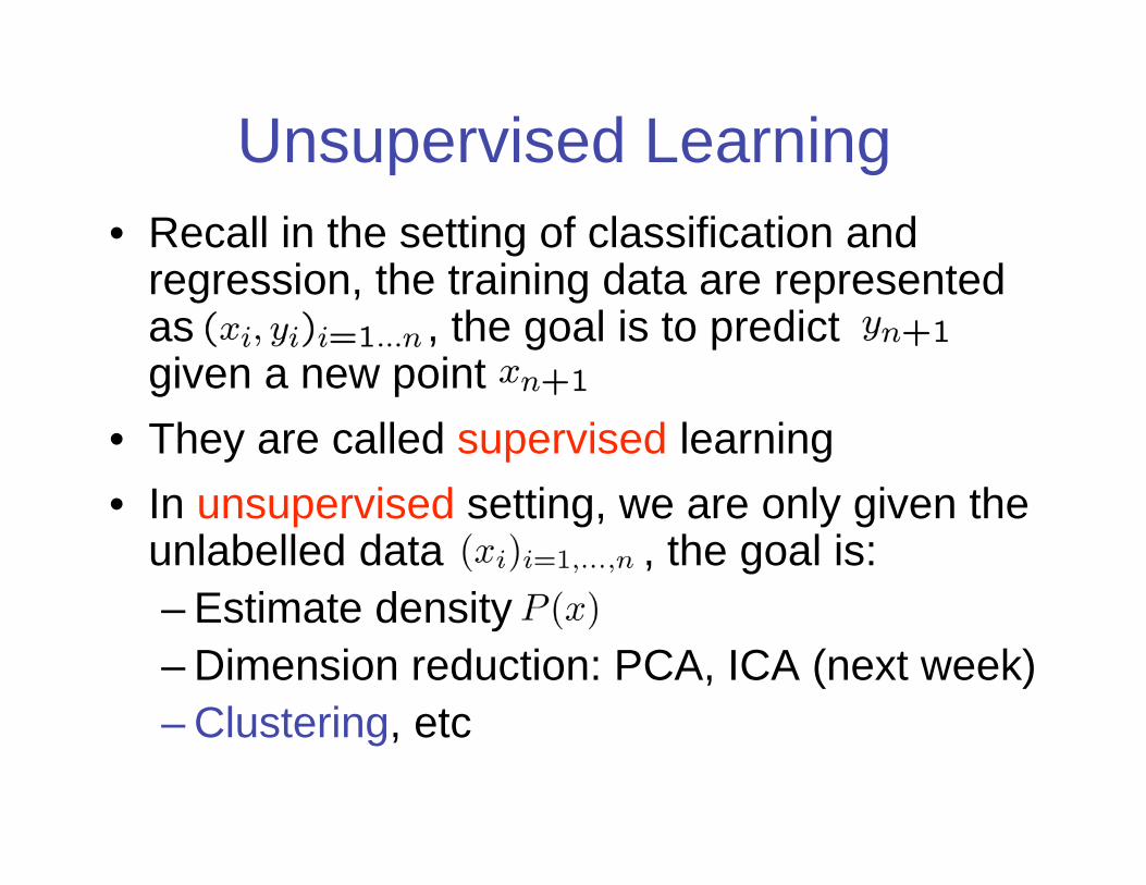
Unsupervised Learning
• Recall in the setting of classification andregression, the training data are representedas , the goal is to predictgiven a new point
• They are called supervised learning
• In unsupervised setting, we are only given theunlabelled data , the goal is:
– Estimate density
– Dimension reduction: PCA, ICA (next week)
– Clustering, etc

What is Clustering?
• Roughly speaking, clustering analysis yields a datadescription in terms of clusters or groups of datapoints that posses strong internal similarity
– a dissimilarity function between objects– an algorithm that operates on the function

What is Clustering?
• Unlike in supervised setting, there is no clear
measure of success for clustering algorithms;
people usually resort to heuristic argument to
judge the quality of the results, e.g. Rand index
(see web supplement for more details)
• Nevertheless, clustering methods are widely used
to perform exploratory data analysis (EDA) in the
early stages of data analysis and gain some
insight into the nature or structure of data

Application of Clustering
• Image segmentation: decompose the image into
regions with coherent color and texture inside them
• Search result clustering: group the search result set
and provide a better user interface (Vivisimo)
• Computational biology: group homologous protein
sequences into families; gene expression data
analysis
• Signal processing: compress the signal by using
codebook derived from vector quantization (VQ)

Outline• Introduction
– Unsupervised learning
– What is clustering? Application
• Dissimilarity (similarity) of objects
• Clustering algorithm
– K-means, VQ, K-medoids
– Gaussian mixture model (GMM), EM
– Hierarchical clustering
– Spectral clustering

Dissimilarity of objects
• The natural question now is: how should we measurethe dissimilarity between objects?
– fundamental to all clustering methods
– usually from subject matter consideration
– not necessarily a metric (i.e. triangle inequalitydoesn’t hold)
– possible to learn the dissimilarity from data (later)
• Similarities can be turned into dissimilarities by
applying any monotonically decreasing transformation

Dissimilarity Based on Attributes
• Most of time, data have measurements onattributes
• Define dissimilarities between attribute values
– common choice:
• Combine the attribute dissimilarities to the objectdissimilarity, using the weighted average
• The choice of weights is also a subject matter
consideration; but possible to learn from data (later)

Dissimilarity Based on Attributes
• Setting all weights equal does not give all attributesequal influence on the overall dissimilarity of objects!
• An attribute’s influence depends on its contribution tothe average object dissimilarity
• Setting gives all attributes equal influencein characterizing overall dissimilarity between objects
average dissimilarity of jth attribute

Dissimilarity Based on Attributes
• For instance, for squared error distance, theaverage dissimilarity of jth attribute is twice thesample estimate of the variance
• The relative importance of each attribute isproportional to its variance over the data set
• Setting (equivalent to standardizing thedata) is not always helpful since attributes mayenter dissimilarity to a different degree
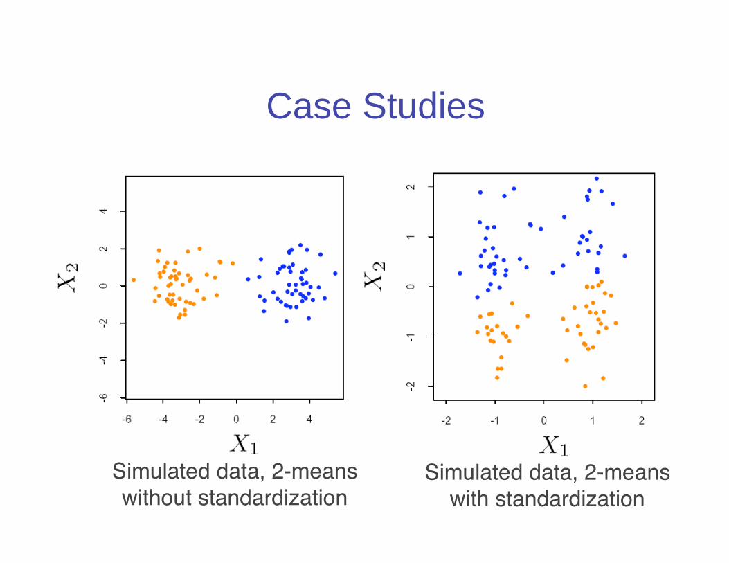
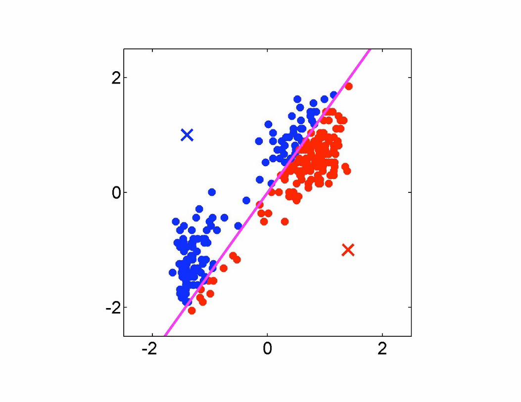
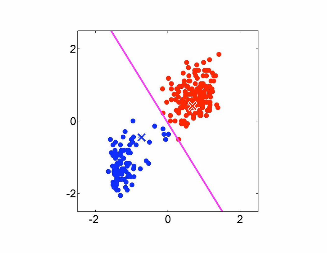
Case Studies
Simulated data, 2-meanswithout standardization
Simulated data, 2-meanswith standardization

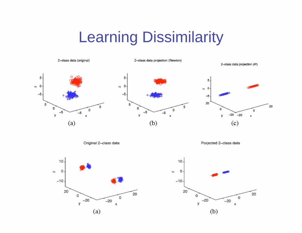
Learning Dissimilarity
• Specifying an appropriate dissimilarity is far more important thanchoice of clustering algorithm
• Suppose a user indicates certain objects are considered by themto be “similar”:
• Consider learning a dissimilarity of form
– If A is diagonal,it corresponds to learn different weights for different
attributes
– Generally, A parameterizes a family of Mahalanobis distance
• Leaning such a dissimilarity is equivalent to finding a rescaling of
data; replace by
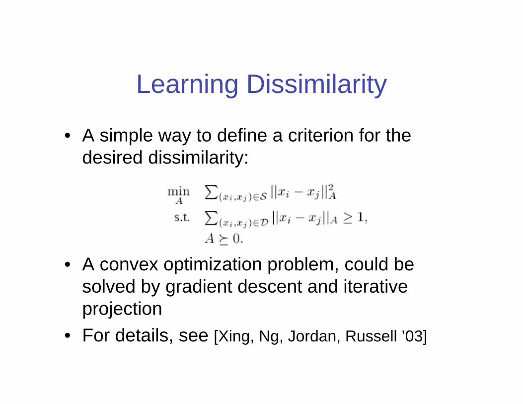
Learning Dissimilarity
• A simple way to define a criterion for the
desired dissimilarity:
• A convex optimization problem, could be
solved by gradient descent and iterative
projection
• For details, see [Xing, Ng, Jordan, Russell ’03]
Learning Dissimilarity

Outline• Introduction
– Unsupervised learning
– What is clustering? Application
• Dissimilarity (similarity) of objects
• Clustering algorithm
– K-means, VQ, K-medoids
– Gaussian mixture model (GMM), EM
– Hierarchical clustering
– Spectral clustering

Old Faithful Data Set
Duration of eruption (minutes)
Time
between
eruptions
(minutes)

K-means
• Idea: represent a data set in terms of K
clusters, each of which is summarized by a
prototype
– Usually applied to Euclidean distance (possibly
weighted, only need to rescale the data)
• Each data is assigned to one of K clusters
– Represented by responsibilities
such that for all data indices i
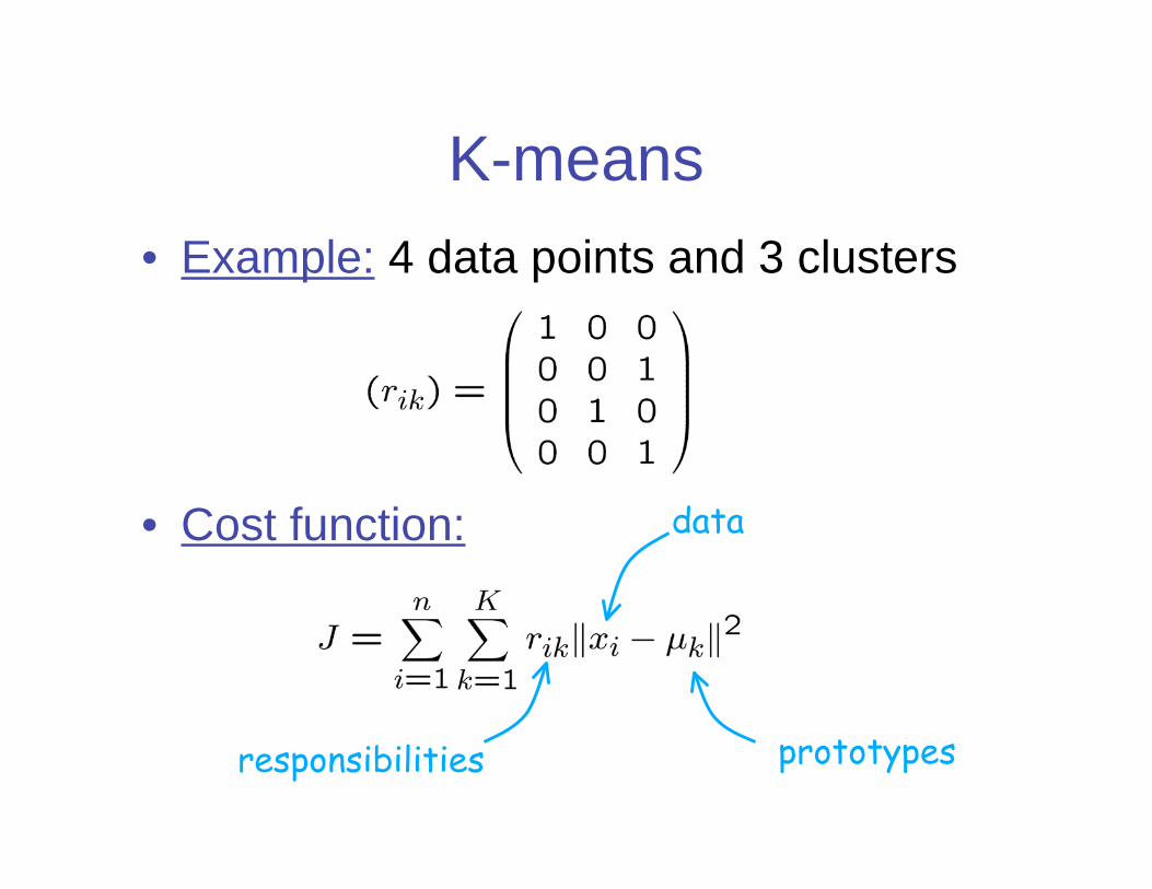
K-means
• Example: 4 data points and 3 clusters
• Cost function:
prototypesresponsibilities
data

Minimizing the Cost Function• Chicken and egg problem, have to resort to iterative
method
• E-step: minimize w.r.t.
– assigns each data point to nearest prototype
• M-step: minimize w.r.t– gives
– each prototype set to the mean of points in thatcluster
• Convergence guaranteed since there is a finite numberof possible settings for the responsibilities
• only finds local minima, should start the algorithm withmany different initial settings


How to Choose K?
• In some cases it is known apriori from problem
domain
• Generally, it has to be be estimate from data and
usually selected by some heuristics in practice
• The cost function J generally decrease with
increasing K
• Idea: Assume that K* is the right number
– We assume that for K<K* each estimated cluster
contains a subset of true underlying groups
– For K>K* some natural groups must be split
– Thus we assume that for K<K* the cost function falls
substantially, afterwards not a lot more

K*
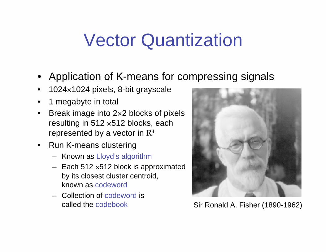
Vector Quantization
• Application of K-means for compressing signals• 1024 1024 pixels, 8-bit grayscale
• 1 megabyte in total
• Break image into 2 2 blocks of pixels
resulting in 512 512 blocks, each
represented by a vector in R4
• Run K-means clustering
– Known as Lloyd’s algorithm
– Each 512 512 block is approximated
by its closest cluster centroid,
known as codeword
– Collection of codeword is
called the codebook Sir Ronald A. Fisher (1890-1962)

Vector Quantization
• Application of K-means for compressing signals• 1024 1024 pixels, 8-bit grayscale
• 1 megabyte in total
• Storage requirement
– K 4 real numbers for the codebook
(negligible)
– log2K bits for storing the code for
each block (can also use variable
length code)
– The ratio is:
– K = 200, the ratio is 0.239K =200
2log /(4 8)K
# pixels per block # bits per pixel inuncompressed image
# bits per block incompressed image

Vector Quantization
• Application of K-means for compressing signals• 1024 1024 pixels, 8-bit grayscale
• 1 megabyte in total
• Storage requirement
– K 4 real numbers for the codebook
(negligible)
– log2K bits for storing the code for
each block (can also use variable
length code)
– The ratio is:
– K = 4, the ratio is 0.063K = 4
2log /(4 8)K
# pixels per block # bits per pixel inuncompressed image
# bits per block incompressed image

K-medoids
• K-means algorithm is sensitive to outliers– An object with an extremely large distance from others
may substantially distort the results, i.e., centroid is notnecessarily inside a cluster
• Idea: instead of using mean of data points within the
clusters, prototypes of clusters are restricted to be
one of the points assigned to the cluster (medoid)– given responsibilities (assignments of points to clusters),
find one of the point within the cluster that minimizes totaldissimilarity to other points in that cluster
• Generally, computation of a cluster prototype
increases from n to n2

Limitations of K-means
• Hard assignments of data points to clusters– Small shift of a data point can flip it to a different
cluster
– Solution: replace hard clustering of K-means withsoft probabilistic assignments (GMM)
• Hard to choose the value of K
– As K is increased, the cluster memberships canchange in an arbitrary way, the resulting clustersare not necessarily nested
– Solution: hierarchical clustering

The Gaussian Distribution
• Multivariate Gaussian
• Maximum likelihood estimation
mean covariance

Gaussian Mixture
• Linear combination of Gaussians
• To generate a data point:– first pick one of the components with probability
– then draw a sample from that component
• Each data is generated by one of K Gaussians, a
latent variable is associated
with each ,
where
parameters to be estimated
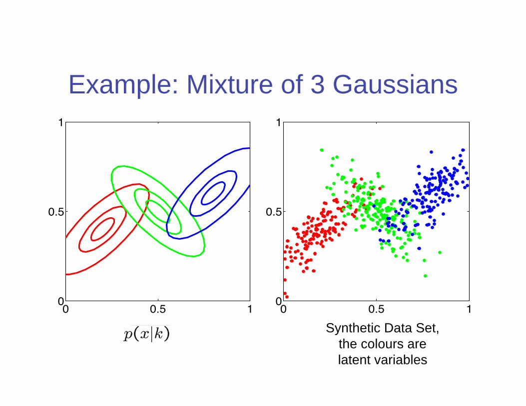
Example: Mixture of 3 Gaussians
0 0.5 10
0.5
1
(a)0 0.5 10
0.5
1
(a)Synthetic Data Set,
the colours are
latent variables
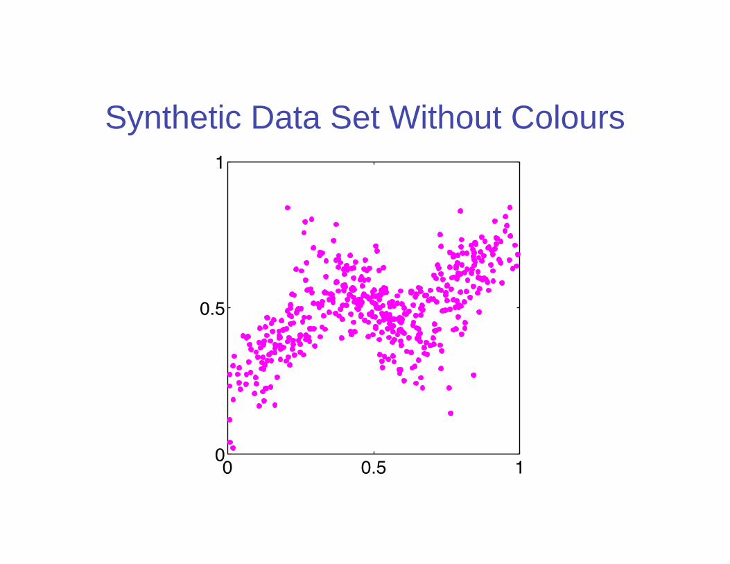
Synthetic Data Set Without Colours
0 0.5 10
0.5
1
(b)

Fitting the Gaussian Mixture• Given the complete data set
– the complete log likelihood
– trivial closed-form solution: fit each component to
the corresponding set of data points
• Without knowing values of latent variables, we
have to maximize the incomplete log likelihood:
– Sum over components appears inside the logarithm,
no closed-form solution
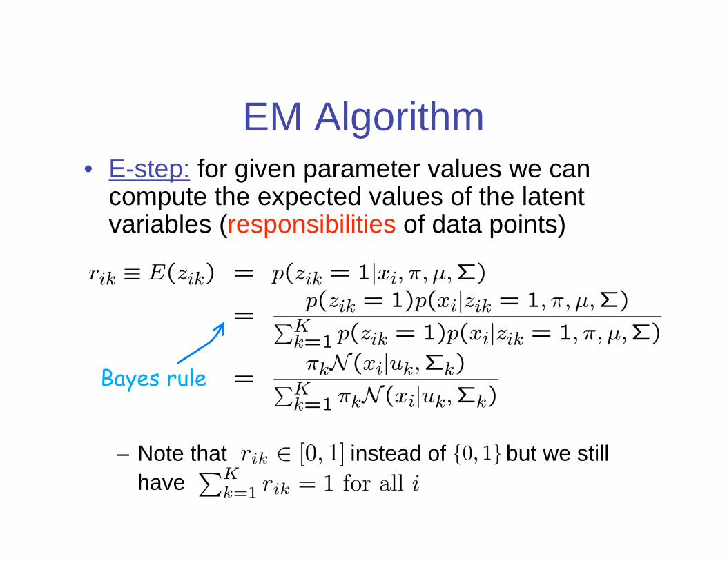
EM Algorithm• E-step: for given parameter values we can
compute the expected values of the latentvariables (responsibilities of data points)
– Note that instead of but we still
have
Bayes rule

EM Algorithm
• M-step: maximize the expected complete log
likelihood
– update parameters:
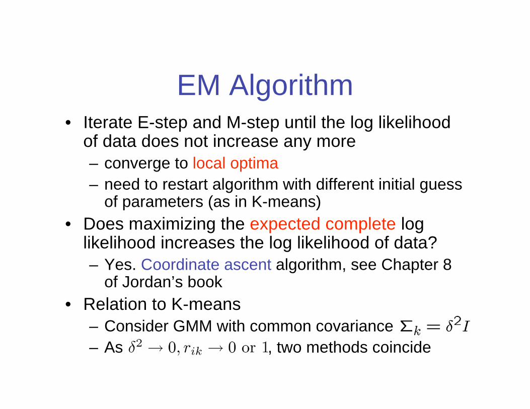
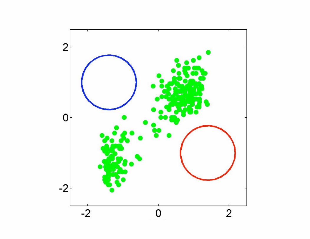
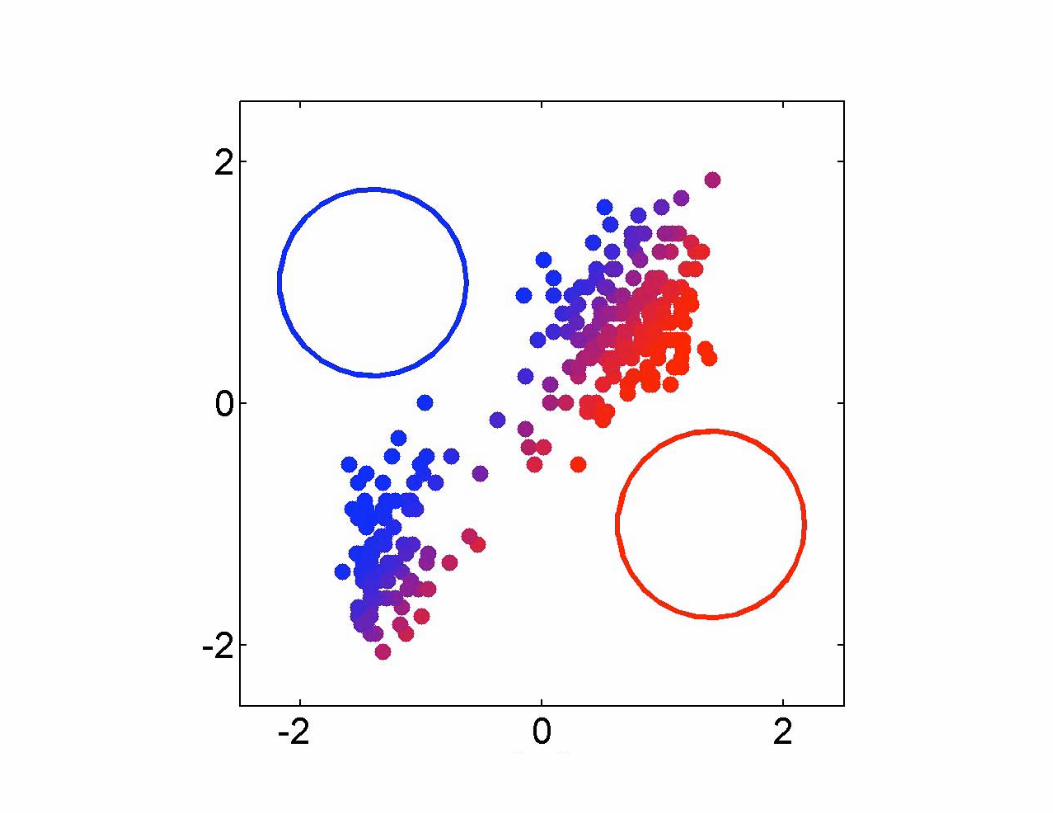
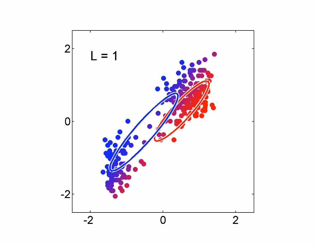
EM Algorithm• Iterate E-step and M-step until the log likelihood
of data does not increase any more
– converge to local optima
– need to restart algorithm with different initial guessof parameters (as in K-means)
• Does maximizing the expected complete loglikelihood increases the log likelihood of data?
– Yes. Coordinate ascent algorithm, see Chapter 8of Jordan’s book
• Relation to K-means
– Consider GMM with common covariance
– As , two methods coincide


Hierarchical Clustering
• Does not require a preset number of clusters
• Organize the clusters in an hierarchical way
• Produces a rooted (binary) tree (dendrogram)
Step 0 Step 1 Step 2 Step 3 Step 4
b
d
c
e
aa b
d e
c d e
a b c d e
Step 4 Step 3 Step 2 Step 1 Step 0
agglomerative
divisive

Hierarchical Clustering• Two kinds of strategy
– Bottom-up (agglomerative): recursively merge two groups with
the smallest between-cluster dissimilarity (defined later on)
– Top-down (divisive): in each step, split a least coherent cluster
(e.g. largest diameter); splitting a cluster is also a clustering
problem (usually done in a greedy way); less popular than
bottom-up way
Step 0 Step 1 Step 2 Step 3 Step 4
b
d
c
e
aa b
d e
c d e
a b c d e
Step 4 Step 3 Step 2 Step 1 Step 0
agglomerative
divisive

Hierarchical Clustering
• User can choose a cut through the hierarchy to
represent the most natural division into clusters
– e.g, choose the cut where intergroup dissimilarity
exceeds some threshold
Step 0 Step 1 Step 2 Step 3 Step 4
b
d
c
e
aa b
d e
c d e
a b c d e
Step 4 Step 3 Step 2 Step 1 Step 0
agglomerative
divisive
3 2
Hierarchical Clustering
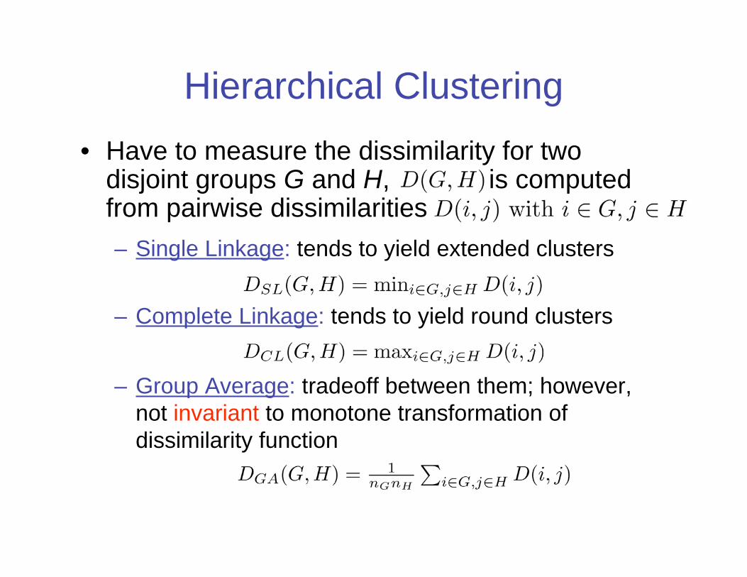
• Have to measure the dissimilarity for twodisjoint groups G and H, is computedfrom pairwise dissimilarities
– Single Linkage: tends to yield extended clusters
– Complete Linkage: tends to yield round clusters
– Group Average: tradeoff between them; however,
not invariant to monotone transformation of
dissimilarity function

Example: Human Tumor Microarray Data
• 6830 64 matrix of real numbers
• Rows correspond to genes,
columns to tissue samples
• Cluster rows (genes) can deduce
functions of unknown genes from
known genes with similar
expression profiles
• Cluster columns (samples) can
identify disease profiles: tissues
with similar disease should yield
similar expression profiles
Gene expression matrix
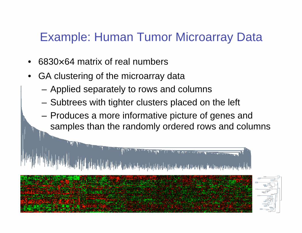
Example: Human Tumor Microarray Data
• 6830 64 matrix of real numbers
• GA clustering of the microarray data
– Applied separately to rows and columns
– Subtrees with tighter clusters placed on the left
– Produces a more informative picture of genes and
samples than the randomly ordered rows and columns

Spectral Clustering
• Idea: use the top eigenvectors of a matrix
derived from distance between data
points
• Too many versions of spectral clustering
algorithms
– has roots in spectral graph partitioning
– only look at one version by Ng, Jordan and
Weiss
– see website for more papers and softwares

Spectral Clustering
• Given a set of points , we’d like tocluster them into k clusters– Form an affinity matrix where
– Define
– Find k largest eigenvectors of L, concatenate them
columnwise to obtain
– Form the matrix Y by normalizing each row of X tohave unit length
– Think of n rows of Y as a new representation oforiginal n data points; cluster them into k clustersusing K-means

Example: Two circles

Example: Two circles

Analysis of algorithm (Ideal case)• In ideal case, say there are 3 clusters that are
infinitely far away from each other, then the affinity
matrix becomes:
• The eigenvalues and eigenvectors of L are the union
of eigenvalues and eigenvectors of its block (the
latter padded appropriately with zeros)
– From spectral graph theory, we know that each block
has a strictly positive principal eigenvector with
eigenvalue 1, the next eigenvalue is strictly less than 1
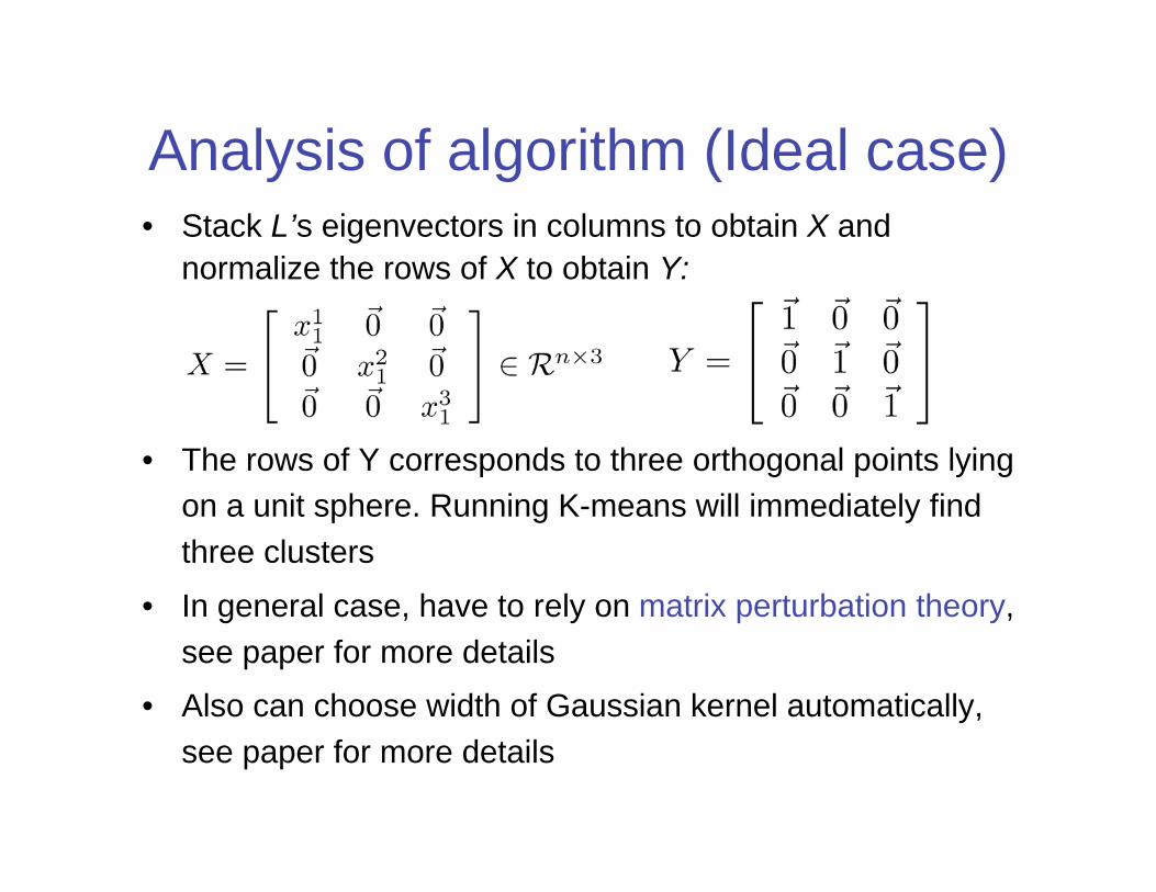
Analysis of algorithm (Ideal case)• Stack L’s eigenvectors in columns to obtain X and
normalize the rows of X to obtain Y:
• The rows of Y corresponds to three orthogonal points lying
on a unit sphere. Running K-means will immediately find
three clusters
• In general case, have to rely on matrix perturbation theory,
see paper for more details
• Also can choose width of Gaussian kernel automatically,
see paper for more details