ARTICLE IN PRESS

Deep-Sea Research II 56 (2009) 554–577

Contents lists available at ScienceDirect

Deep-Sea Research II

0967-06

doi:10.1

� Corr

E-m

journal homepage: www.elsevier.com/locate/dsr2

Climatological mean and decadal change in surface ocean pCO2, and netsea–air CO2 flux over the global oceans

Taro Takahashi a,�, Stewart C. Sutherland a, Rik Wanninkhof b, Colm Sweeney c, Richard A. Feely d,David W. Chipman e, Burke Hales f, Gernot Friederich g, Francisco Chavez g, Christopher Sabine d,Andrew Watson h, Dorothee C.E. Bakker h, Ute Schuster h, Nicolas Metzl i, Hisayuki Yoshikawa-Inoue j,Masao Ishii k, Takashi Midorikawa k, Yukihiro Nojiri l, Arne Kortzinger m, Tobias Steinhoff m,Mario Hoppema n, Jon Olafsson o, Thorarinn S. Arnarson o, Bronte Tilbrook p, Truls Johannessen q,Are Olsen q, Richard Bellerby q, C.S. Wong r, Bruno Delille s, N.R. Bates t, Hein J.W. de Baar u

a Lamont-Doherty Earth Observatory, Columbia University, 61 Route 9W, PO Box 1000, Palisades, NY 10964-8000, USAb Atlantic Oceanographic and Meteorological Laboratory, National Oceanographic and Atmospheric Administration, Miami, FL, USAc Earth System Research Laboratory, National Oceanographic and Atmospheric Administration, Boulder, CO, USAd Pacific Marine Environmental Laboratory, National Oceanographic and Atmospheric Administration, Seattle, WA, USAe 103 Reach Road, Harpswell, ME, USAf College of Oceanic and Atmospheric Sciences, Oregon State University, Corvallis, OR, USAg Monterey Bay Aquarium Research Institute, Moss Landing, CA, USAh School of Environmental Sciences, University of East Anglia, Norwich, UKi Laboratoire d’Oceanographie et du Climat, LOCEAN/IPSL, CNRS, Universite Pierre et Marie Curie, Paris, Francej Graduate School of Environmental Earth Science, Hokkaido University, Sapporo, Japank Meteorological Research Institute, Tsukuba, Japanl National Institute for Environmental Studies, Tsukuba, Japanm Leibniz Institute of Marine Sciences, Kiel, Germanyn Alfred Wegener Institute, Bremerhaven, Germanyo Marine Research Institute and University of Iceland, Reykjavik, Icelandp Wealth from Oceans, CSIRO National Research Flagship, and the Antarctic Climate and Ecosystem Cooperative Research Center, Hobart, Australiaq Bjerknes Centre for Climate Research, University of Bergen, Norwayr Institute of Ocean Sciences, Fisheries and Oceans Canada, Sidney, B.C., Canadas Universite de Liege, Liege, Belgiumt Bermuda Institute of Ocean Studies, Bermudau Royal Netherlands Institute of Sea Research, Den Burg, The Netherlands

a r t i c l e i n f o

Available online 16 December 2008

Keywords:

Carbon dioxide

Partial pressure

Surface ocean

Global ocean

Sea–air flux

45/$ - see front matter & 2008 Elsevier Ltd. A

016/j.dsr2.2008.12.009

esponding author.

ail address: taka@ldeo.columbia.edu (T. Takah

a b s t r a c t

A climatological mean distribution for the surface water pCO2 over the global oceans in non-El Nino

conditions has been constructed with spatial resolution of 41 (latitude) �51 (longitude) for a reference

year 2000 based upon about 3 million measurements of surface water pCO2 obtained from 1970 to

2007. The database used for this study is about 3 times larger than the 0.94 million used for our earlier

paper [Takahashi et al., 2002. Global sea–air CO2 flux based on climatological surface ocean pCO2, and

seasonal biological and temperature effects. Deep-Sea Res. II, 49, 1601–1622]. A time-trend analysis

using deseasonalized surface water pCO2 data in portions of the North Atlantic, North and South Pacific

and Southern Oceans (which cover about 27% of the global ocean areas) indicates that the surface water

pCO2 over these oceanic areas has increased on average at a mean rate of 1.5matm y�1 with basin-

specific rates varying between 1.270.5 and 2.170.4matm y�1. A global ocean database for a single

reference year 2000 is assembled using this mean rate for correcting observations made in different

years to the reference year. The observations made during El Nino periods in the equatorial Pacific and

those made in coastal zones are excluded from the database.

Seasonal changes in the surface water pCO2 and the sea-air pCO2 difference over four climatic zones

in the Atlantic, Pacific, Indian and Southern Oceans are presented. Over the Southern Ocean seasonal ice

zone, the seasonality is complex. Although it cannot be thoroughly documented due to the limited

extent of observations, seasonal changes in pCO2 are approximated by using the data for under-ice

waters during austral winter and those for the marginal ice and ice-free zones.

ll rights reserved.

ashi).

ARTICLE IN PRESS

T. Takahashi et al. / Deep-Sea Research II 56 (2009) 554–577 555

The net air–sea CO2 flux is estimated using the sea–air pCO2 difference and the air–sea gas transfer

rate that is parameterized as a function of (wind speed)2 with a scaling factor of 0.26. This is estimated

by inverting the bomb 14C data using Ocean General Circulation models and the 1979–2005 NCEP-DOE

AMIP-II Reanalysis (R-2) wind speed data. The equatorial Pacific (141N–141S) is the major source for

atmospheric CO2, emitting about +0.48 Pg-C y�1, and the temperate oceans between 141 and 501 in the

both hemispheres are the major sink zones with an uptake flux of �0.70 Pg-C y�1 for the northern

and �1.05 Pg-C y�1 for the southern zone. The high-latitude North Atlantic, including the Nordic Seas

and portion of the Arctic Sea, is the most intense CO2 sink area on the basis of per unit area, with a mean

of �2.5 tons-C month�1 km�2. This is due to the combination of the low pCO2 in seawater and high gas

exchange rates. In the ice-free zone of the Southern Ocean (501–621S), the mean annual flux is small

(�0.06 Pg-C y�1) because of a cancellation of the summer uptake CO2 flux with the winter release

of CO2 caused by deepwater upwelling. The annual mean for the contemporary net CO2 uptake flux over

the global oceans is estimated to be �1.670.9 Pg-C y�1, which includes an undersampling correction to

the direct estimate of �1.470.7 Pg-C y�1. Taking the pre-industrial steady-state ocean source of

0.470.2 Pg-C y�1 into account, the total ocean uptake flux including the anthropogenic CO2 is estimated

to be �2.071.0 Pg-C y�1 in 2000.

& 2008 Elsevier Ltd. All rights reserved.

1. Introduction

Recent rapid accumulation of CO2 in the atmosphere is one ofthe major environmental concerns because of its potentialeffects on the future global climate. Anticipated warming andassociated environmental changes including sea-level rise wouldadversely affect the socio-economic stability of human societyand global terrestrial–marine ecosystems. The results of variousindependent lines of study show that the present net global oceanCO2 uptake (not including the pre-industrial steady-state flux) is1.5–2.0 Pg-C y�1 (Pg ¼ Peta grams ¼ 1015 g ¼ 1 Giga ton), whichcorresponds to about 25% of the industrial emissions of about7 Pg-C y�1 (Bender et al., 2005; Gloor et al., 2003; Gruber andSarmiento, 2002; Gurney et al., 2004; Jacobson et al., 2007a, b;Keeling and Garcia, 2002; Mikaloff-Fletcher et al., 2006; Patraet al., 2005; Quay et al., 2003; Sabine et al., 2004; Sarmiento et al.,2000; Takahashi et al., 2002). Accurate assessment of the sea–airCO2 flux and its time–space variability is important informationfor the improvement of our understanding of the global carboncycle and the prognosis for the future atmospheric CO2 concen-tration. In this paper, we summarize the measurements of partialpressure of CO2 in surface waters made 1970–2006 by a largenumber of international investigators over the global oceans andpresent estimates for the sea–air CO2 flux.

The difference between the partial pressure of CO2 in seawaterand that in the overlying air, DpCO2 ¼ [(pCO2)sw–(pCO2)air], is thethermochemical driving potential for the net transfer of CO2

across the sea surface. For example, when (pCO2)air is greater than(pCO2)sw, DpCO2 is negative and atmospheric CO2 is taken up bythe seawater. The net CO2 flux across sea surface can be estimatedby multiplying the DpCO2 by the CO2 gas transfer coefficient,which depends primarily on the degree of turbulence near theinterface. Using this principle, the first set of global surface waterpCO2 data, consisting of about 0.24 million pCO2 measurements,was assembled and the climatological mean distributions ofDpCO2 and sea–air CO2 flux were estimated (Takahashi et al.,1997) using the time–space interpolation method based on a2-dimensional diffusion–advection transport equation (Takahashiet al., 1995). In the course of the following several years, thedatabase were more than tripled in size to about 0.94 millionmeasurements by 2002, and the second improved version thatincluded the climatological mean monthly distribution of surfacewater pCO2 and sea–air flux in the reference year 1995 waspublished (Takahashi et al., 2002). The database have since beenincreased by another three-fold to 3 million (pCO2)sw measure-ments. As a result, we have been able to obtain a more reliableestimate for interannual changes in surface water pCO2. This

paper presents the new results for the climatological meandistribution of surface water pCO2 and net sea–air CO2 flux overthe global oceans in the reference year of 2000 representing meannon-El Nino conditions.

2. Measurements of surface water pCO2 and database

2.1. Data sources and database

The database used for this study consists of about 3.0 millionmeasurements of surface water pCO2 obtained since the early1970s. About 0.2 million measurements made in the equatorialPacific, 101N–101S, during the five El Nino periods (1982–1983,1986–1987, 1991–1994, 1997–1998, 2002–2003 and 2004–2005)and about 0.2 million made in the coastal waters (within about200 km from the shore) are excluded from the total database of3.4 million. The remaining 3.0 million (pCO2)sw values used forthe analysis represent open-ocean environments during non-ElNino conditions. This is supplemented by an equal number ofother associated data such as SST and salinity. The earlierpublications that describe the data are listed in Takahashi et al.(1993, 2002), and the original data files for more recentobservations are available from the authors of this paper. Sinceinvestigators processed the field observations somewhat differ-ently, we have recomputed all the data using the proceduresdescribed below in order to produce a uniform database. Theentire database including the coastal and El Nino periodequatorial Pacific data (Takahashi et al., 2008) are available atthe Carbon Dioxide Information and Analysis Center at theOak Ridge National Laboratory, Oak Ridge, TN (LDEO database(NDP-088) at http://cdiac.ornl.gov/oceans/doc.html).

Although pCO2 may be computed using TCO2, alkalinity and/orpH, it depends on the choice of dissociation constants used.Therefore, we accepted in the database only the pCO2 valuesmeasured directly using the air–water equilibration method, inwhich two or more standard gas mixtures (not counting purenitrogen or CO2-free air) were used for analyzer calibrations.

2.2. Method for measurements

The (pCO2)sw data used in this study were determined using aturbulent water–air equilibration method modified from the basicdesigns developed during the 1957–1959 International Geophy-sical Year (Takahashi, 1961; Keeling et al., 1965; Broecker andTakahashi, 1966), or of the membrane-equilibrator method (Haleset al., 2004). A volume of carrier gas is equilibrated with seawater

ARTICLE IN PRESS

T. Takahashi et al. / Deep-Sea Research II 56 (2009) 554–577556

(closed or continuously flowing), and the concentration of CO2 inthe equilibrated carrier gas is measured using a CO2 gas analyzer,either by infrared CO2 absorption or gas chromatographicanalyses. The analyzers are calibrated using two or more referencegas mixtures, of which the CO2 molar mixing ratios are traceableto either the WMO standards maintained by C.D. Keeling or thereference gases certified by the Earth System Research Laboratoryof NOAA. When a dried carrier gas is analyzed, the pCO2 inseawater at equilibration temperature, Teq, is computed using

ðpCO2Þsw ¼ XCO2ðPeq � PwÞ (1)

where XCO2 is the mole fraction of CO2 in dry air; Peq is the totalpressure of carrier gas in the equilibration chamber; and Pw is thewater vapor pressure at the temperature of equilibration, Teq, andsalinity. When the CO2 mixing ratios in the wet carrier gas isdetermined, Pw is set at zero. When an equilibrator is located in anenclosed shipboard laboratory and is open to the room air, Peq isthe ambient pressure in the laboratory. In some data sets, Peq isnot reported for an equilibrator operated in an enclosed space. Insuch cases, Peq is assumed to be the reported barometric pressureat sea surface plus 3 mb, that represents an overpressure normallymaintained inside a ship. This correction increases the (pCO2)sw

value by about 1matm.To correct the (pCO2)sw measured at Teq to the in situ seawater

temperature, Tin situ, a constant-chemistry temperature effect,(q ln pCO2/q T) ¼ 0.0433–8.7�10�5T (1C), which was determinedfor a North Atlantic surface water sample (Takahashi et al., 1993),is used. Eq. (2) is an integrated form of the equation above:

ðpCO2Þsw at T in situ ¼ ½ðpCO2Þsw at Teq�Expf0:0433ðT in situ � TeqÞ

� 4:35� 10�5½ðT in situÞ

2� ðTeqÞ

2�g (2)

In our previous publication (Takahashi et al., 2002), a meancoefficient of 0.0423 1C�1 (Takahashi et al., 1993) was used insteadof Eq. (2). If (Tin situ–Teq) is less than 2 1C, Eq. (2) yields pCO2 valuesvirtually indistinguishable from the previous ones. Since tem-perature changes for continuous underway systems are com-monly less than this, the corrections made using the constantcoefficient do not require changes. Only those measured fordiscrete water samples are subject to change up to about 3matm.For the reasons discussed in Section 2.3, we take the reported‘‘bulk’’ water temperature as Tin situ to represent the sea-surfacecondition. The average precision of individual pCO2 measure-ments thus obtained is estimated to be 73matm at a reported‘‘bulk’’ water temperature.

Since the data reported by the participating groups had beenprocessed using different computational schemes, all the data arerecomputed using Eqs. (1) and (2) in order to remove biases. In thecalculation, CO2 gas is treated as ideal in the range of pressuresencountered in this study, and the effects of non-ideal mixingbehaviors of CO2 molecules in air due to CO2–H2O–N2–O2

molecular interactions are neglected since they are small(o1matm) and are inferred from correlations among the heat ofmixing and other thermodynamic parameters for various mole-cular species (Weiss and Price, 1980).

2.3. Temperature of ocean water

The upper several meters of the ocean are thermally stratifieddepending upon heat balance and turbulence. Since pCO2 inseawater depends sensitively on temperature, we need to select aTin situ in Eq. (2), that is critical to the sea–air CO2 gas transfer. Inthe skin layer regime (o500mm), where conductive and diffusiveheat transfer processes are dominant, the layer is cooled due toevaporation; in the sub-skin regime (�1 cm to a few meters),where diffusive and viscous processes are important, the water is

warmed by short-wave solar radiation during the day time; andthe bulk mixing layer (a few to several meters) is governedprimarily by turbulent mixing. Donlon et al. (2002) compared thebulk water temperatures measured at a depth of 5 m concurrentlywith the mean skin temperature observations using a shipboardinfrared radiometer during six cruises between 501N and 501S inthe Atlantic and Pacific Oceans. They observed that, at wind speedsexceeding 6 m s�1, the skin temperatures were cooler than the bulkwater temperatures (measured at 5 m) by �0.1770.07 1C for boththe day- and night-time conditions. At lower wind speeds, skintemperatures of 2 1C or more warmer than bulk temperatures wereobserved during day-time, but not during night-time.

Sarmiento and Sundquist (1992) and Robertson and Watson(1992) proposed that, since skin layer of the oceans is a few tenthsof degree cooler than the bulk water, the skin layer pCO2 should belower by as much as 1% than that at the bulk water temperature,thus increasing the air-to-sea CO2 flux by as much as 30% (or0.1–0.7 Pg-C y�1). On the other hand, McGillis and Wanninkhof(2006) pointed out that, since molecular diffusivities for gases andsalt are nearly two orders of magnitude smaller than the thermaldiffusivity, the thickness of the diffusive layer for gases should bean order of magnitude smaller than that for the thermal diffusivelayer. Hence, the difference between the (CO2)aq (and hence pCO2)in the skin- and sub-skin layers should be an order of magnitudesmaller than that estimated on the basis of the thermal skin layerthickness. The effect of skin cooling on pCO2, therefore, should bemuch smaller than previously proposed. Furthermore, Zhang andCai (2007) consider that, as a result of smaller salt diffusivity thanthermal diffusivity in seawater, the skin cooling caused byevaporation may be accompanied with a much thinner salty-skinlayer. Since the pCO2 of seawater decreases with cooling andincreases with salinity (q ln pCO2/q ln Sal ¼ 0.94, Takahashi et al.,1993), the effect of skin cooling should be nearly cancelled by thatof salty skin. Since the skin layer thickness decreases inverselyproportional to wind speed (Saunders, 1967; Fairall et al., 1996), itseffect on pCO2 should be reduced over high wind speed areas ofthe oceans (such as the southern high wind belt 40–551S).Therefore, the effect of skin layer cooling on seawater pCO2 isconsidered to be negligibly small.

In addition to the effect of skin layer cooling, solar heatingaffects the temperature of the upper few meters of tropical oceans(Fairall et al., 1996). Satellite-borne microwave measurementsshow that, over tropical regions under low wind speed conditions,the day-time temperatures of the upper few meters of waterexceed the bulk water temperatures (those assembled by Reynoldsand Smith (1994)) as much as 2.8 1C (Gentemann et al., 2003). Theday-time warming would influence the net daily sea–air flux ofCO2 especially in tropical oceans (McNeil and Merlivat, 1996; Wardet al., 2004). On the other hand, for this study, most of the pCO2

were measured during day and night continuously for a depthrange of 1–7 m, and the pCO2 and bulk water temperature data areaveraged over a 41�51 box area without differentiating the day-and night-time measurements. Hence, the pCO2 bias resultingfrom the day-time warming is considered minimal.

As discussed above, the pCO2 that represents the interfacelayer with the atmosphere cannot be defined unequivocally on thebasis of the measurements in our database. Nevertheless, basedon the available information, we judge that the effect of thermalskin layer on pCO2 is negligibly small, and that the bias due todiurnal temperature changes is minimized by the averaging oflarge number of day- and night-time measurements. In this study,therefore, the pCO2 value measured at the ‘‘bulk’’ water tempera-ture is taken as that for the sea-surface value. As the surface-layereffects should become further clarified in the future, they shouldbe taken into consideration in order to reduce systematic errors insea–air pCO2 differences.

ARTICLE IN PRESS

T. Takahashi et al. / Deep-Sea Research II 56 (2009) 554–577 557

2.4. Atmospheric pCO2

The atmospheric pCO2, (pCO2)air, in the reference year 2000 iscomputed using:

ðpCO2Þair ¼ XCO2ðPbaro � PswÞ (3)

where Pbaro is the barometric pressure at sea surface, and Psw isthe water vapor pressure at the temperature and salinity formixed layer water. The following values are used: the weeklymean XCO2 data in dry air from the GLOBALVIEW—CO2 Database(2006); for Psw, 100% humidity at SST (temperature of bulk mixedlayer water) and surface water salinity from the NOAA’s Atlas ofSurface Marine Data (1994); and for Pbaro, the climatologicalmonthly mean barometric pressure at sea surface from the NCEPReanalysis data (2001). The sea–air pCO2 difference, DpCO2, isthen computed using

DpCO2 ¼ ½ðpCO2Þsw corrected to the year 2000�

� ½ðpCO2Þair in 2000� (4)

Since CO2 is assumed to be an ideal gas for both (pCO2)sw and(pCO2)air, the small effects of non-ideality should cancel due todifferencing for pCO2. Positive DpCO2 values indicate that the sea

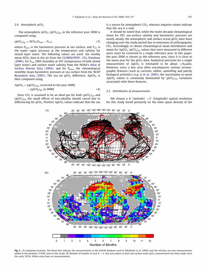
Fig. 1. (A) Sampling locations. The black dots indicate the measurements in the 0.94 M

added to the database (3.0 M) used in this study. (B) Number of months in each 41�51 b

the early 1970s. White areas have no measurements.

is a source for atmospheric CO2, whereas negative values indicatethat the sea is a sink.

It should be noted that, while the multi-decadal climatologicalmean for SST, sea-surface salinity and barometric pressure arenearly steady, the atmospheric and surface ocean pCO2 have beenchanging over the study period due to emissions of anthropogenicCO2. Accordingly, to obtain climatological mean distribution andmean for DpCO2, (pCO2)sw values that were measured in differentyears must be corrected to a single reference year. In this paper,the year 2000 is chosen as the reference year, since it is close tothe mean year for the pCO2 data. Analytical precision for a singlemeasurement of DpCO2 is estimated to be about 74matm.However, since a box area often encompasses various oceano-graphic features (such as currents, eddies, upwelling and patchybiological activities) (e.g. Li et al., 2005), the uncertainty in meanDpCO2 values is commonly dominated by (pCO2)sw variationsassociated with these features.

2.5. Distribution of measurements

We choose a 41 (latitude) �51 (longitude) spatial resolutionfor this study based primarily on the time–space density of the

database used in Takahashi et al. (2002) and the red dots are new measurements

ox area where at least one surface water pCO2 measurement has been made since

ARTICLE IN PRESS

T. Takahashi et al. / Deep-Sea Research II 56 (2009) 554–577558

observations. While smaller box areas would help to resolvenarrow oceanographic features such as the Gulf Stream andequatorial currents, they would reduce the number of observa-tions made in a box during different seasons and hence fail todefine seasonal variation. Even at this box size, observations madein several years have to be combined to define seasonal variability.Multi-year composite maps summarizing the sampling locationsand the number of months, in which at least one measurementwas made since 1970 in each box, are shown in Figs. 1A and B. Thelatter map shows that, of a total of 1759 boxes, about 30% of theboxes have measurements spanning 6 or more months, and 50% ofthe boxes have measurements spanning 3 or less months. Whilemost boxes in the Northern Hemisphere have observations in 6 ormore months, many in the Southern Hemisphere oceans south of201S have data only in 3 or less months. The Drake Passage areasthat are being investigated as part of the Long Term EcosystemResearch (LTER) program along the Antarctic Peninsula are theonly southern high-latitude boxes that have 12-month data.

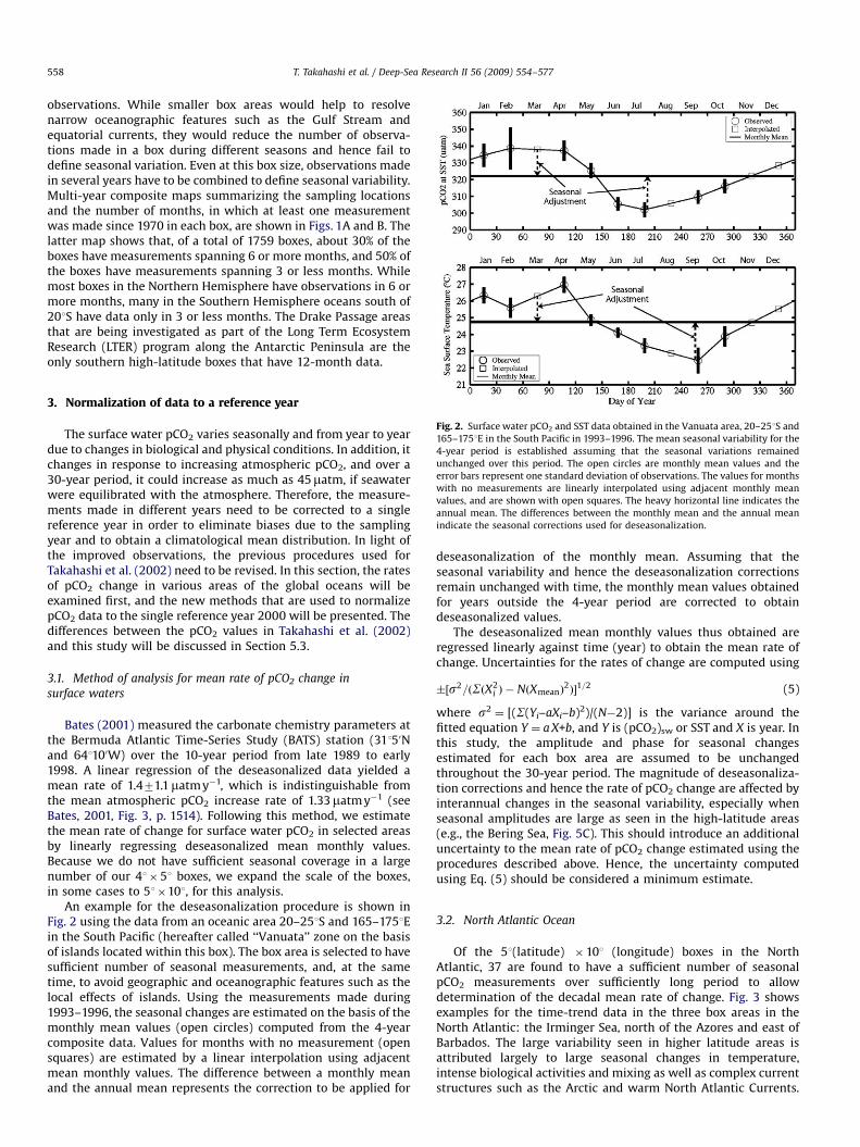
Fig. 2. Surface water pCO2 and SST data obtained in the Vanuata area, 20–251S and

165–1751E in the South Pacific in 1993–1996. The mean seasonal variability for the

4-year period is established assuming that the seasonal variations remained

unchanged over this period. The open circles are monthly mean values and the

error bars represent one standard deviation of observations. The values for months

with no measurements are linearly interpolated using adjacent monthly mean

values, and are shown with open squares. The heavy horizontal line indicates the

annual mean. The differences between the monthly mean and the annual mean

indicate the seasonal corrections used for deseasonalization.

3. Normalization of data to a reference year

The surface water pCO2 varies seasonally and from year to yeardue to changes in biological and physical conditions. In addition, itchanges in response to increasing atmospheric pCO2, and over a30-year period, it could increase as much as 45matm, if seawaterwere equilibrated with the atmosphere. Therefore, the measure-ments made in different years need to be corrected to a singlereference year in order to eliminate biases due to the samplingyear and to obtain a climatological mean distribution. In light ofthe improved observations, the previous procedures used forTakahashi et al. (2002) need to be revised. In this section, the ratesof pCO2 change in various areas of the global oceans will beexamined first, and the new methods that are used to normalizepCO2 data to the single reference year 2000 will be presented. Thedifferences between the pCO2 values in Takahashi et al. (2002)and this study will be discussed in Section 5.3.

3.1. Method of analysis for mean rate of pCO2 change in

surface waters

Bates (2001) measured the carbonate chemistry parameters atthe Bermuda Atlantic Time-Series Study (BATS) station (31150Nand 641100W) over the 10-year period from late 1989 to early1998. A linear regression of the deseasonalized data yielded amean rate of 1.471.1matm y�1, which is indistinguishable fromthe mean atmospheric pCO2 increase rate of 1.33matm y�1 (seeBates, 2001, Fig. 3, p. 1514). Following this method, we estimatethe mean rate of change for surface water pCO2 in selected areasby linearly regressing deseasonalized mean monthly values.Because we do not have sufficient seasonal coverage in a largenumber of our 41�51 boxes, we expand the scale of the boxes,in some cases to 51�101, for this analysis.

An example for the deseasonalization procedure is shown inFig. 2 using the data from an oceanic area 20–251S and 165–1751Ein the South Pacific (hereafter called ‘‘Vanuata’’ zone on the basisof islands located within this box). The box area is selected to havesufficient number of seasonal measurements, and, at the sametime, to avoid geographic and oceanographic features such as thelocal effects of islands. Using the measurements made during1993–1996, the seasonal changes are estimated on the basis of themonthly mean values (open circles) computed from the 4-yearcomposite data. Values for months with no measurement (opensquares) are estimated by a linear interpolation using adjacentmean monthly values. The difference between a monthly meanand the annual mean represents the correction to be applied for

deseasonalization of the monthly mean. Assuming that theseasonal variability and hence the deseasonalization correctionsremain unchanged with time, the monthly mean values obtainedfor years outside the 4-year period are corrected to obtaindeseasonalized values.

The deseasonalized mean monthly values thus obtained areregressed linearly against time (year) to obtain the mean rate ofchange. Uncertainties for the rates of change are computed using

�½s2=ðSðX2i Þ � NðXmeanÞ

2Þ�1=2 (5)

where s2¼ [(S(Yi–aXi–b)2)/(N�2)] is the variance around the

fitted equation Y ¼ a X+b, and Y is (pCO2)sw or SST and X is year. Inthis study, the amplitude and phase for seasonal changesestimated for each box area are assumed to be unchangedthroughout the 30-year period. The magnitude of deseasonaliza-tion corrections and hence the rate of pCO2 change are affected byinterannual changes in the seasonal variability, especially whenseasonal amplitudes are large as seen in the high-latitude areas(e.g., the Bering Sea, Fig. 5C). This should introduce an additionaluncertainty to the mean rate of pCO2 change estimated using theprocedures described above. Hence, the uncertainty computedusing Eq. (5) should be considered a minimum estimate.

3.2. North Atlantic Ocean

Of the 51(latitude) �101 (longitude) boxes in the NorthAtlantic, 37 are found to have a sufficient number of seasonalpCO2 measurements over sufficiently long period to allowdetermination of the decadal mean rate of change. Fig. 3 showsexamples for the time-trend data in the three box areas in theNorth Atlantic: the Irminger Sea, north of the Azores and east ofBarbados. The large variability seen in higher latitude areas isattributed largely to large seasonal changes in temperature,intense biological activities and mixing as well as complex currentstructures such as the Arctic and warm North Atlantic Currents.

ARTICLE IN PRESS

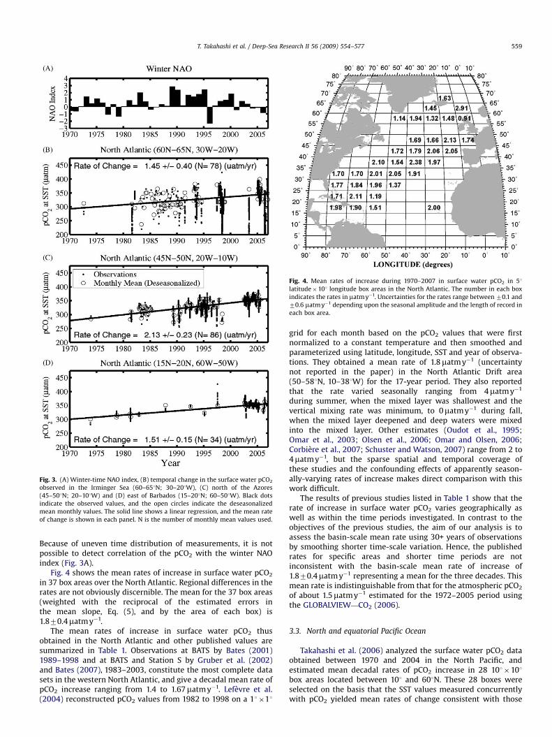
Fig. 3. (A) Winter-time NAO index, (B) temporal change in the surface water pCO2

observed in the Irminger Sea (60–651N; 30–201W), (C) north of the Azores

(45–501N; 20–101W) and (D) east of Barbados (15–201N; 60–501W). Black dots

indicate the observed values, and the open circles indicate the deseasonalized

mean monthly values. The solid line shows a linear regression, and the mean rate

of change is shown in each panel. N is the number of monthly mean values used.

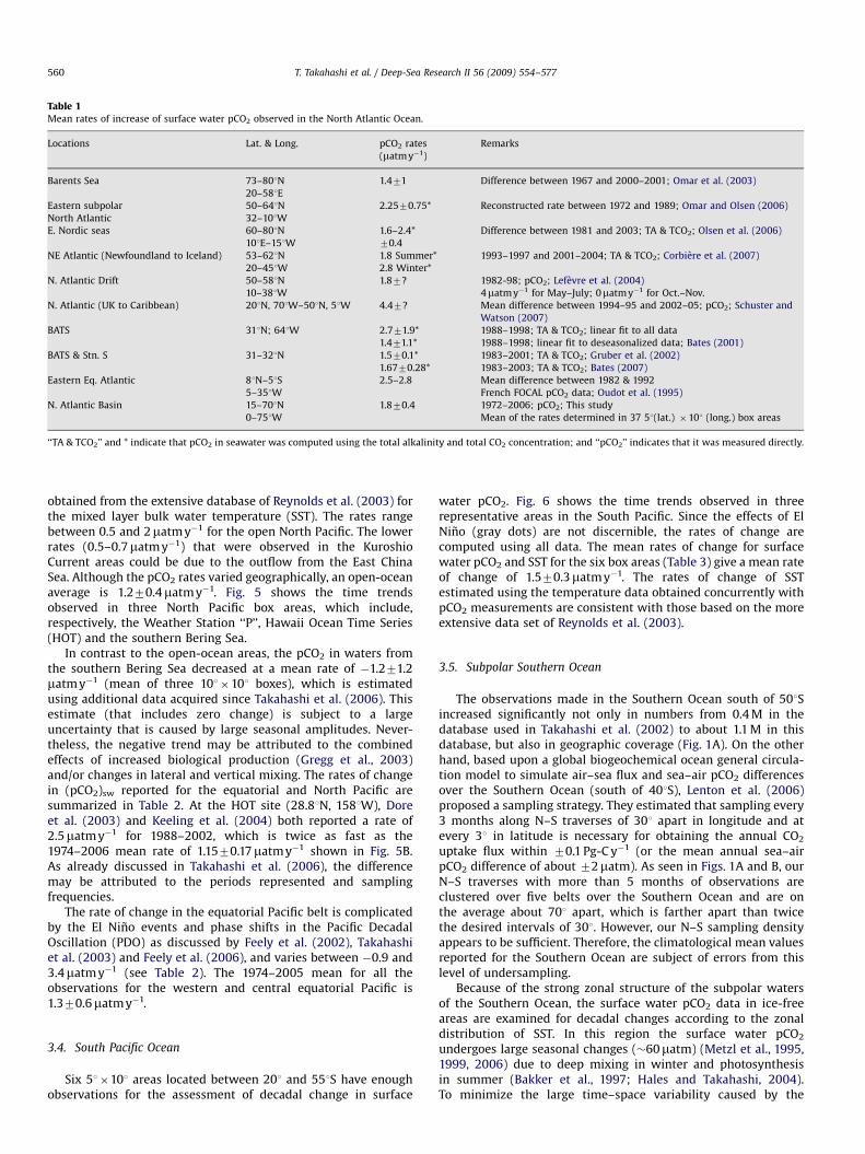
Fig. 4. Mean rates of increase during 1970–2007 in surface water pCO2 in 51

latitude�101 longitude box areas in the North Atlantic. The number in each box

indicates the rates in matm y�1. Uncertainties for the rates range between 70.1 and

70.6 matm y�1 depending upon the seasonal amplitude and the length of record in

each box area.

T. Takahashi et al. / Deep-Sea Research II 56 (2009) 554–577 559

Because of uneven time distribution of measurements, it is notpossible to detect correlation of the pCO2 with the winter NAOindex (Fig. 3A).

Fig. 4 shows the mean rates of increase in surface water pCO2

in 37 box areas over the North Atlantic. Regional differences in therates are not obviously discernible. The mean for the 37 box areas(weighted with the reciprocal of the estimated errors inthe mean slope, Eq. (5), and by the area of each box) is1.870.4matm y�1.

The mean rates of increase in surface water pCO2 thusobtained in the North Atlantic and other published values aresummarized in Table 1. Observations at BATS by Bates (2001)1989–1998 and at BATS and Station S by Gruber et al. (2002)and Bates (2007), 1983–2003, constitute the most complete datasets in the western North Atlantic, and give a decadal mean rate ofpCO2 increase ranging from 1.4 to 1.67matm y�1. Lefevre et al.(2004) reconstructed pCO2 values from 1982 to 1998 on a 11�11

grid for each month based on the pCO2 values that were firstnormalized to a constant temperature and then smoothed andparameterized using latitude, longitude, SST and year of observa-tions. They obtained a mean rate of 1.8matm y�1 (uncertaintynot reported in the paper) in the North Atlantic Drift area(50–581N, 10–381W) for the 17-year period. They also reportedthat the rate varied seasonally ranging from 4matm y�1

during summer, when the mixed layer was shallowest and thevertical mixing rate was minimum, to 0matm y�1 during fall,when the mixed layer deepened and deep waters were mixedinto the mixed layer. Other estimates (Oudot et al., 1995;Omar et al., 2003; Olsen et al., 2006; Omar and Olsen, 2006;Corbiere et al., 2007; Schuster and Watson, 2007) range from 2 to4matm y�1, but the sparse spatial and temporal coverage ofthese studies and the confounding effects of apparently season-ally-varying rates of increase makes direct comparison with thiswork difficult.

The results of previous studies listed in Table 1 show that therate of increase in surface water pCO2 varies geographically aswell as within the time periods investigated. In contrast to theobjectives of the previous studies, the aim of our analysis is toassess the basin-scale mean rate using 30+ years of observationsby smoothing shorter time-scale variation. Hence, the publishedrates for specific areas and shorter time periods are notinconsistent with the basin-scale mean rate of increase of1.870.4matm y�1 representing a mean for the three decades. Thismean rate is indistinguishable from that for the atmospheric pCO2

of about 1.5matm y�1 estimated for the 1972–2005 period usingthe GLOBALVIEW—CO2 (2006).

3.3. North and equatorial Pacific Ocean

Takahashi et al. (2006) analyzed the surface water pCO2 dataobtained between 1970 and 2004 in the North Pacific, andestimated mean decadal rates of pCO2 increase in 28 101�101box areas located between 101 and 601N. These 28 boxes wereselected on the basis that the SST values measured concurrentlywith pCO2 yielded mean rates of change consistent with those

ARTICLE IN PRESS

Table 1Mean rates of increase of surface water pCO2 observed in the North Atlantic Ocean.

Locations Lat. & Long. pCO2 rates

(matm y�1)

Remarks

Barents Sea 73–801N 1.471 Difference between 1967 and 2000–2001; Omar et al. (2003)

20–581E

Eastern subpolar 50–641N 2.2570.75* Reconstructed rate between 1972 and 1989; Omar and Olsen (2006)

North Atlantic 32–101W

E. Nordic seas 60–801N 1.6–2.4* Difference between 1981 and 2003; TA & TCO2; Olsen et al. (2006)

101E–151W 70.4

NE Atlantic (Newfoundland to Iceland) 53–621N 1.8 Summer* 1993–1997 and 2001–2004; TA & TCO2; Corbiere et al. (2007)

20–451W 2.8 Winter*

N. Atlantic Drift 50–581N 1.87? 1982-98; pCO2; Lefevre et al. (2004)

10–381W 4matm y�1 for May–July; 0matm y�1 for Oct.–Nov.

N. Atlantic (UK to Caribbean) 201N, 701W–501N, 51W 4.47? Mean difference between 1994–95 and 2002–05; pCO2; Schuster and

Watson (2007)

BATS 311N; 641W 2.771.9* 1988–1998; TA & TCO2; linear fit to all data

1.471.1* 1988–1998; linear fit to deseasonalized data; Bates (2001)

BATS & Stn. S 31–321N 1.570.1* 1983–2001; TA & TCO2; Gruber et al. (2002)

1.6770.28* 1983–2003; TA & TCO2; Bates (2007)

Eastern Eq. Atlantic 81N–51S 2.5–2.8 Mean difference between 1982 & 1992

5–351W French FOCAL pCO2 data; Oudot et al. (1995)

N. Atlantic Basin 15–701N 1.870.4 1972–2006; pCO2; This study

0–751W Mean of the rates determined in 37 51(lat.) �101 (long.) box areas

‘‘TA & TCO2’’ and * indicate that pCO2 in seawater was computed using the total alkalinity and total CO2 concentration; and ‘‘pCO2’’ indicates that it was measured directly.

T. Takahashi et al. / Deep-Sea Research II 56 (2009) 554–577560

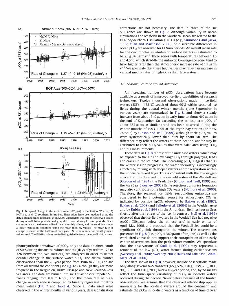
obtained from the extensive database of Reynolds et al. (2003) forthe mixed layer bulk water temperature (SST). The rates rangebetween 0.5 and 2matm y�1 for the open North Pacific. The lowerrates (0.5–0.7matm y�1) that were observed in the KuroshioCurrent areas could be due to the outflow from the East ChinaSea. Although the pCO2 rates varied geographically, an open-oceanaverage is 1.270.4matm y�1. Fig. 5 shows the time trendsobserved in three North Pacific box areas, which include,respectively, the Weather Station ‘‘P’’, Hawaii Ocean Time Series(HOT) and the southern Bering Sea.

In contrast to the open-ocean areas, the pCO2 in waters fromthe southern Bering Sea decreased at a mean rate of �1.271.2matm y�1 (mean of three 101�101 boxes), which is estimatedusing additional data acquired since Takahashi et al. (2006). Thisestimate (that includes zero change) is subject to a largeuncertainty that is caused by large seasonal amplitudes. Never-theless, the negative trend may be attributed to the combinedeffects of increased biological production (Gregg et al., 2003)and/or changes in lateral and vertical mixing. The rates of changein (pCO2)sw reported for the equatorial and North Pacific aresummarized in Table 2. At the HOT site (28.81N, 1581W), Doreet al. (2003) and Keeling et al. (2004) both reported a rate of2.5matm y�1 for 1988–2002, which is twice as fast as the1974–2006 mean rate of 1.1570.17matm y�1 shown in Fig. 5B.As already discussed in Takahashi et al. (2006), the differencemay be attributed to the periods represented and samplingfrequencies.

The rate of change in the equatorial Pacific belt is complicatedby the El Nino events and phase shifts in the Pacific DecadalOscillation (PDO) as discussed by Feely et al. (2002), Takahashiet al. (2003) and Feely et al. (2006), and varies between �0.9 and3.4matm y�1 (see Table 2). The 1974–2005 mean for all theobservations for the western and central equatorial Pacific is1.370.6matm y�1.

3.4. South Pacific Ocean

Six 51�101 areas located between 201 and 551S have enoughobservations for the assessment of decadal change in surface

water pCO2. Fig. 6 shows the time trends observed in threerepresentative areas in the South Pacific. Since the effects of ElNino (gray dots) are not discernible, the rates of change arecomputed using all data. The mean rates of change for surfacewater pCO2 and SST for the six box areas (Table 3) give a mean rateof change of 1.570.3matm y�1. The rates of change of SSTestimated using the temperature data obtained concurrently withpCO2 measurements are consistent with those based on the moreextensive data set of Reynolds et al. (2003).

3.5. Subpolar Southern Ocean

The observations made in the Southern Ocean south of 501Sincreased significantly not only in numbers from 0.4 M in thedatabase used in Takahashi et al. (2002) to about 1.1 M in thisdatabase, but also in geographic coverage (Fig. 1A). On the otherhand, based upon a global biogeochemical ocean general circula-tion model to simulate air–sea flux and sea–air pCO2 differencesover the Southern Ocean (south of 401S), Lenton et al. (2006)proposed a sampling strategy. They estimated that sampling every3 months along N–S traverses of 301 apart in longitude and atevery 31 in latitude is necessary for obtaining the annual CO2

uptake flux within 70.1 Pg-C y�1 (or the mean annual sea–airpCO2 difference of about 72matm). As seen in Figs. 1A and B, ourN–S traverses with more than 5 months of observations areclustered over five belts over the Southern Ocean and are onthe average about 701 apart, which is farther apart than twicethe desired intervals of 301. However, our N–S sampling densityappears to be sufficient. Therefore, the climatological mean valuesreported for the Southern Ocean are subject of errors from thislevel of undersampling.

Because of the strong zonal structure of the subpolar watersof the Southern Ocean, the surface water pCO2 data in ice-freeareas are examined for decadal changes according to the zonaldistribution of SST. In this region the surface water pCO2

undergoes large seasonal changes (�60matm) (Metzl et al., 1995,1999, 2006) due to deep mixing in winter and photosynthesisin summer (Bakker et al., 1997; Hales and Takahashi, 2004).To minimize the large time–space variability caused by the

ARTICLE IN PRESS

Fig. 5. Temporal change in the surface water pCO2 (A) in the Station ‘‘P’’ area, (B)

HOT area and (C) southern Bering Sea. These plots have been updated using the

data obtained since Takahashi et al. (2006). Black dots indicate the observed values

during non-El Nino periods, and gray dots those during El Nino periods. Open

circles indicate the deseasonalized mean monthly values, and the solid line shows

a linear regression computed using the mean monthly values. The mean rate of

change is shown at the bottom of each panel. N is the number of monthly mean

values used. The El Nino values are indistinguishable from the non-El Nino values.

T. Takahashi et al. / Deep-Sea Research II 56 (2009) 554–577 561

photosynthetic drawdown of pCO2, only the data obtained southof 501S during the austral winter months (days of year from 172 to326 between the two solstices) are analyzed in order to detectdecadal change in the surface water pCO2. The austral winterobservations span the 20-year period from 1986 to 2006, and arefrom all around the continent (see Fig. 1A), although they are morefrequent in the Kerguelen, Drake Passage and New Zealand-RossSea areas. The data are binned into six 11C-wide circumpolar SSTzones ranging from 0.8 to 6.5 1C, and the mean rate of pCO2

change in each zone is computed by linearly regressing monthlymean values (Fig. 7 and Table 4). Since all data used wereobserved in the winter months in various years, deseasonalization

corrections are not necessary. The data in three of the sixSST zones are shown in Fig. 7. Although variability in oceancirculations and ice fields in the Southern Ocean are related to theEl Nino/Southern Oscillation (ENSO) (e.g., Simmonds and Jacka,1995; Yuan and Martinson, 2000), no discernible differences inocean pCO2 are observed for El Nino periods. An overall mean ratefor the circumpolar sub-Antarctic surface waters is estimated tobe 2.170.6matm y�1. Three zones with temperatures between 1.5and 4.5 1C, which straddle the Antarctic Convergence Zone, tend tohave higher rates than the atmospheric increase rate of 1.5matmy�1. We speculate that these high values may reflect an increase invertical mixing rates of high-CO2 subsurface waters.

3.6. Seasonal ice zone around Antarctica

An increasing number of pCO2 observations have becomeavailable as a result of improved ice-field capabilities of researchicebreakers. Twelve thousand observations made in ice-fieldwaters (SSTp�1.75 1C) south of about 601S within seasonal icefields during the austral winter months (June–September invarious years) are summarized in Fig. 8, and show a steadyincrease from about 340matm in early June to about 410matm inthe end of September, far exceeding the atmospheric pCO2 ofabout 357matm. A similar trend has been observed during thewinter months of 1993–1995 at the Prydz Bay station (681340S,781550E) by Gibson and Trull (1999), although their pCO2 valueswere systematically lower than ours by about 50matm. Thedifference may reflect the waters at their location, and/or may beattributed to their pCO2 values that were calculated using TCO2

and pH measurements.These data in Fig. 8 represent the under-ice waters, which may

be exposed to the air and exchange CO2 through polynyas, leadsand cracks in the ice fields. The increasing pCO2 suggests that, asthe winter season progresses, the water chemistry is increasinglyaffected by mixing with deeper waters and/or respiration withinthe under-ice mixed layer. This is consistent with the low oxygenconcentrations observed in the ice-field waters of the Weddell Sea(Gordon et al., 1984), the Prydz Bay (Gibson and Trull, 1999) andthe Ross Sea (Sweeney, 2003). Brine rejection during ice formationmay also contribute some high CO2 waters (Nomura et al., 2006).Therefore, the seasonal ice fields surrounding Antarctica areconsidered to be a potential source for atmospheric CO2 asindicated by positive DpCO2 observed by Bakker et al. (1997),Bakker et al. (2008) and Bellerby et al., (2004) in the Weddell gyreand by Rubin et al. (1998) in the Amundsen–Bellingshausen Seasshortly after the retreat of the ice. In contrast, Stoll et al. (1999)observed that the ice-field waters in the Weddell Sea had negativeDpCO2 (30matm below the atmospheric) in early winter ofApril–May 1996, and proposed that the Weddell Sea could be asignificant CO2 sink throughout the winter. The observationspresented in Fig. 8 (i. e. pCO2 4360matm after June) as well as thework cited above do not support their extrapolation of the earlywinter observations into the peak winter months. We speculatethat the observations of Stoll et al. (1999) may represent aremnant of the low pCO2 water formed during earlier seasons(Sweeney et al., 2000; Sweeney, 2003; Hales and Takahashi, 2004;Metzl et al., 2006).

The data shown in Fig. 8, however, include observations madeonly along several N–S transects (65751W, 1707101W, 207101E,907301E and 1207201E) over a 10-year period, and, by no meansreflect the time–space variability of pCO2 in ice-field watersoccurred during the decade. Nevertheless, because of the limitedobservations, we assume that the observed relationship appliesuniversally for the ice-field waters around the continent, andestimate the pCO2 in ice-field waters as a function of time of year

ARTICLE IN PRESS

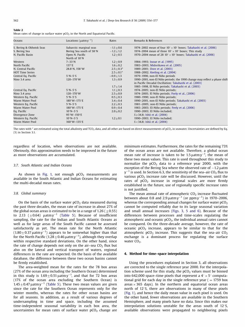
Table 2Mean rates of change in surface water pCO2 in the North and Equatorial Pacific.

Oceans Locations (matm y�1) Rates Remarks & References

S. Bering & Okhotsk Seas Subarctic marginal seas �1.170.6 1974–2002 mean of four 101�101 boxes; Takahashi et al. (2006)

S. Bering Sea Bering Sea south of 581N �1.271.2 1974–2004 mean of three 101�101 boxes; This study

N. Pacific Basin Open N. Pacific 1.270.5 1970–2004 mean of 28 101�101 boxes; Takahashi et al. (2006)

North of 101N

Western 7–331N 1.270.9 1984–1993; Inoue et al. (1995)

North Pacific 1371E 1.670.2 1983–2003; Midorikawa et al. (2005)

N. Central Pacific 28.81N, 1581W 2.570.3* 1989–2001; Dore et al. (2003)

HOT Time Series 2.570.1* 1988–2002; Keeling et al. (2004)

Central Eq. Pacific 51N–51S �0.971.3 1979–1990, non-El Nino periods

Nino 3.4 area 120–1701W 1.370.9 1990–2001, non-El Nino periods; the 1990 change may reflect a phase shift

in Pacific Decadal Oscillation; Takahashi et al. (2003)

1.771.4 1985–1998, El Nino periods; Takahashi et al. (2003)

Central Eq. Pacific 51N–51S 1.170.3 1974–2005; non-El Nino periods;

Nino 3.4 area 120–1701W 2.570.9 1974–2005; El Nino periods; Feely et al., (2006)

Western Eq. Pacific 51N–51S 0.570.3 1980–1990; non-El Nino periods;

Warm Water Pool 1801W–1751E 3.470.4 1990–2001, non-El Nino periods; Takahashi et al. (2003)

Western Eq. Pacific 51N–51S 2.270.3 1981–2005; non-El Nino periods;

Warm Water Pool 1801W–1751E 0.970.4 1983–2003; El-Nino periods; Feely et al. (2006)

Eq. Pacific 101N–51S 2.070.2 1990–2003; El Nino included;

Divergence Zone 951W–1501E SX34.8; Ishii et al. (2004)

Western Eq. Pacific 101N–51S 1.270.1 1990–2003; El Nino included;

Warm Water Pool 1601W–1351E So34.8; Ishii et al. (2004)

The rates with * are estimated using the total alkalinity and TCO2 data, and all other are based on direct measurements of pCO2 in seawater. Uncertainties are defined by Eq.

(5) in Section 3.1.

T. Takahashi et al. / Deep-Sea Research II 56 (2009) 554–577562

regardless of location, when observations are not available.Obviously, this approximation needs to be improved in the futureas more observations are accumulated.

3.7. South Atlantic and Indian Oceans

As shown in Fig. 1, not enough pCO2 measurements areavailable in the South Atlantic and Indian Oceans for estimatingthe multi-decadal mean rates.

3.8. Global summary

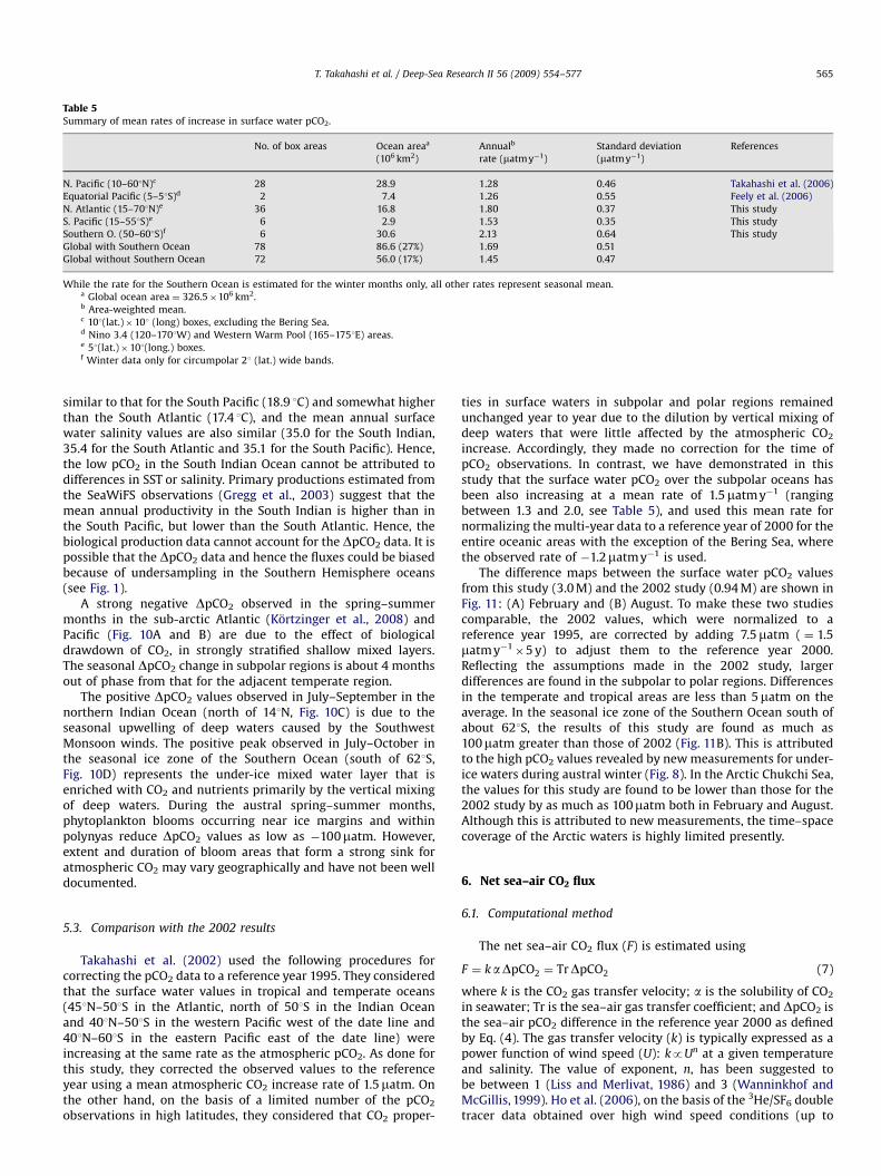
On the basis of the surface water pCO2 data measured duringthe past three decades, the mean rate of increase in about 27% ofthe global ocean areas is estimated to be in a range of 1.26 (70.55)to 2.13 (70.64) matm y�1 (Table 5). Because of insufficientsampling, the rate for the Indian and South Atlantic Oceans aswell as for large areas of the South Pacific cannot be assessedsatisfactorily as yet. The mean rate for the North Atlantic(1.8070.37matm y�1) appears to be somewhat higher than thatfor the North Pacific (1.2870.46matm y�1), although they overlapwithin respective standard deviations. On the other hand, sincethe rate of change depends not only on the air–sea CO2 flux butalso on the lateral and vertical transport of waters, regionaldifferences in the rate are expected. On the basis of the availabledatabase, the difference between these two ocean basins cannotbe firmly established.

The area-weighted mean for the rates for the 78 box areas(27% of the ocean area including the Southern Ocean) determinedin this study is 1.6970.51matm y�1, and that for 72 box areas(17% of the ocean area excluding the Southern Ocean) is1.4570.47matm y�1 (Table 5). These two mean values are givensince the rate for the Southern Ocean represents only for thewinter months, whereas the rates for other ocean basins arefor all seasons. In addition, as a result of various degrees ofundersampling in time and space, including the assumedtime-independent seasonal variability in each box area, theuncertainties for mean rates of surface water pCO2 change are

minimum estimates. Furthermore, the rates for the remaining 73%of the ocean areas are not available. Therefore, a global oceanmean rate of increase is taken to be 1.5matm y�1, the mean ofthese two mean values. This rate is used throughout this study tonormalize the pCO2 data to a reference year 2000, with theexception of the Bering Sea where the observed rate of �1.2matmy�1 is used. In Section 6.3, the sensitivity of the sea–air CO2 flux tovarious pCO2 increase rate will be discussed. However, until therates of pCO2 increase in regional scales are more firmlyestablished in the future, use of regionally specific increase ratesis not justified.

The mean annual rate of atmospheric CO2 increase fluctuatedbetween about 0.8 and 2.9matm y�1 (or ppm y�1) in 1970–2006,whereas the corresponding annual changes for surface water pCO2

cannot be computed reliably due to its large seasonal variationand small annual increases (Figs. 3, 5 and 6). Because of thedifferences between processes and time-scales regulating theatmospheric and oceanic pCO2, the individual annual rates cannotbe compared. On the three-decade average, however, the rate ofoceanic pCO2 increase, appears to be similar to that for theatmospheric pCO2 increase. This suggests that the sea–air CO2

exchange is a dominant process for regulating the surfacewater CO2.

4. Method for time–space interpolation

Using the procedures explained in Section 3, all observationsare corrected to the single reference year 2000. For the interpola-tion scheme used for this study, the pCO2 values must be binnedinto 642,000 space–time pixels that represent a 41�51 computa-tional grid for each day in the single reference year ( ¼ 1759 boxareas�365 days). In the northern and equatorial ocean areasnorth of 121S, there are observations in many of these pixels(Fig. 1), and hence the daily mean value in each pixel is used. Onthe other hand, fewer observations are available in the SouthernHemisphere, and many pixels have no data. Since this makes ourinterpolation solutions unstable for the areas south of 121S,available observations were propagated to neighboring pixels

ARTICLE IN PRESS

Fig. 6. Rates of increase in surface water pCO2 in three areas in the temperate

South Pacific: (A) Vanuata area, (B) Tasmania area and (C) New Zealand area. Solid

dots (black for non-El Nino periods and gray for El Nino periods) indicate

individual measurements, and open circles are the deseasonalized monthly mean

values. The effects of El Nino events are not discernible. The mean annual rate of

change is computed using a linear regression for the deseasonalized mean

monthly values.

T. Takahashi et al. / Deep-Sea Research II 56 (2009) 554–577 563

with no observations by including the values in neighboring areasfor 741 latitude, 751 longitude and 71 day from the center ofa pixel. The mean is computed by weighting a measured valueinversely proportional to its time-space distance from the pixelcenter. This procedure is equivalent of increasing the size of pixelsto four neighboring pixels over 3 days (past, present and future by1 day). After the above procedures are applied, about 50% of thespace–time pixels over the global oceans have measured values.

To estimate pCO2 values in the boxes without observations, aninterpolation equation based on 2-D diffusion–advection trans-port equation for surface waters is used:

dS=dt ¼ Kr2S� ðqS=qx Vxþ qS=qy VyÞ (6)

where r2S ¼ q2S/qx2+q2S/qy2.

S is a scaler quantity, K is lateral eddy diffusivity set at acanonical value of 2000 m2/s for surface waters (Thiele et al.,1986), and Vx and Vy are monthly mean advective velocities forsurface waters. For the advective flow field, the monthly mean ofToggweiler et al. (1989) is used. This equation is discretized onto a51 longitude by 41 latitude spatial grid over the globe, and solvediteratively using a finite difference algorithm (Takahashi et al.,1995, 1997). Material transport across the sea–land interface isassumed to be negligibly small: qS/qx ¼ 0 and qS/qy ¼ 0. Singula-rities at the poles are avoided by the presence of Antarctica in thesouth and by treating the Arctic ice field as land in the north.The surface water pCO2 values are the solutions obtained after500 iterations. This is determined on the basis of behaviors of thetemperature values that are interpolated using the same methoddescribed above.

In this interpolation scheme, the observations are satisfiedexplicitly, and those in pixels that have no observationsare computed by the continuity equation. The effects of internalsources and sinks of CO2, exchange with atmosphere andupwelling of deep waters are considered imbedded in theobserved data, and accordingly, terms for internal source andsink and exchange fluxes are neglected in Eq. (6). While theinterpolation scheme yields daily values, the monthly meanvalues for each box area are presented in this paper.

5. Climatological mean distribution of surface water pCO2

5.1. Global distribution

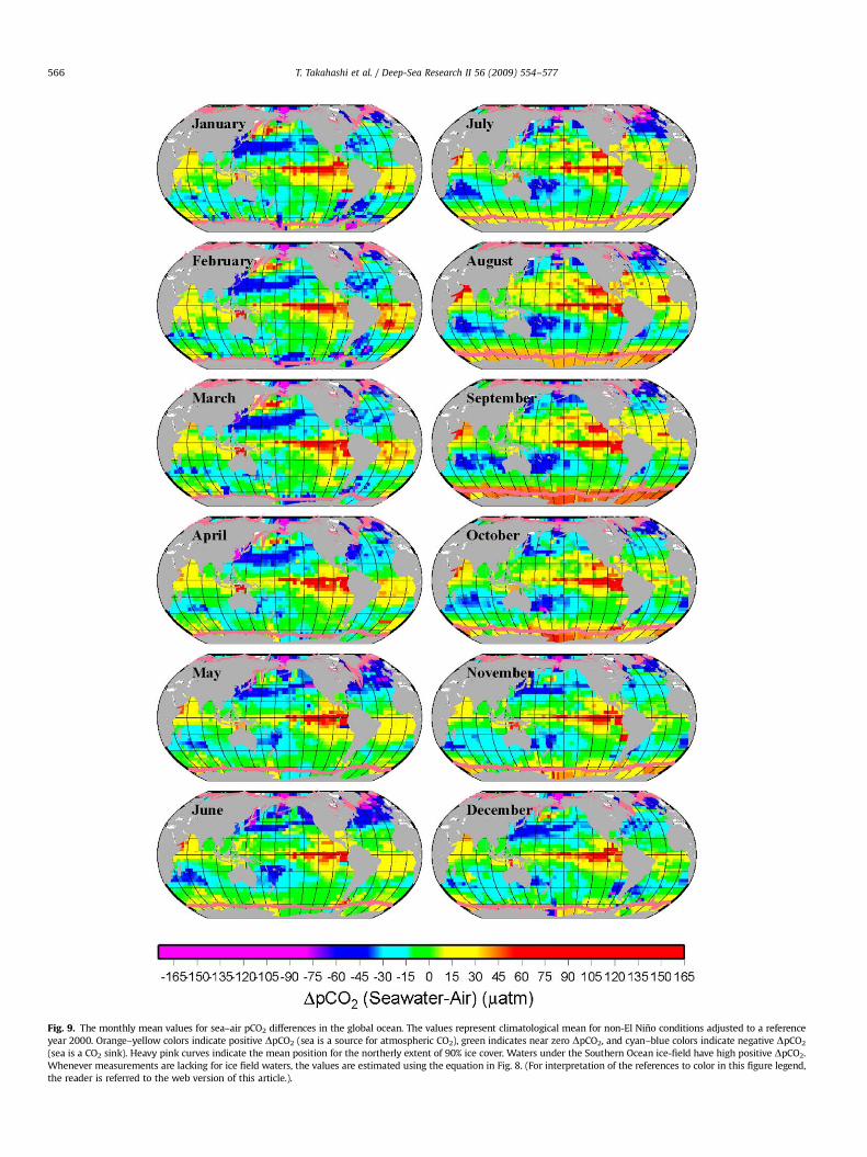
The climatological mean distribution of DpCO2 in each monthfor the reference year 2000 (Fig. 9) is computed using the monthlymean surface water pCO2 values over the global ocean andthe mean monthly atmospheric pCO2 values for the year 2000as described in Section 2. It should be pointed out that anydifferences between the new and the previous maps for thereference years 1990 (Takahashi et al., 1997) and 1995 (Takahashiet al., 2002) do not indicate changes occurred in the oceans from1990 to 2000, but rather reflect primarily the improved databaseas well as the improvements in the normalization method for thereference year as described in Section 3.

5.2. Regional distribution

To show the seasonal and regional changes in DpCO2 moreclearly, monthly mean DpCO2 data are plotted in Fig. 10 for sixclimatic zones in the four ocean basins. The tropical belt(141N–141S) of the oceans has high positive values with littleseasonal variability, indicating that the area is a strong source forCO2 year around. The tropical Pacific (Fig. 10B) has the highestpositive DpCO2 values (annual mean of 27matm), the tropicalAtlantic (Fig. 10A, annual mean of 18matm) next, and the tropicalIndian (Fig. 10C, annual mean of 15matm) the lowest. Thetemperate Atlantic and Pacific (14–501 in the both hemispheres)exhibit large seasonal changes, positive DpCO2 in warm summermonths and negative values in colder winter months reflectingthe dominant effect on (pCO2)sw of seasonal SST changes.However, the peak-to-peak amplitude for the temperate NorthAtlantic is about 42matm, and is somewhat larger than 37matmfor the temperate North Pacific. Since the mean seasonalamplitudes for SST are similar in these two ocean areas (5.7 and5.8 1C), the difference in DpCO2 amplitudes cannot be attributed toSST, and may reflect differences in biological environments suchas a greater supply of nitrate by the nitrification of atmosphericnitrogen in the North Atlantic (Capone et al., 2005). Seasonal

ARTICLE IN PRESS

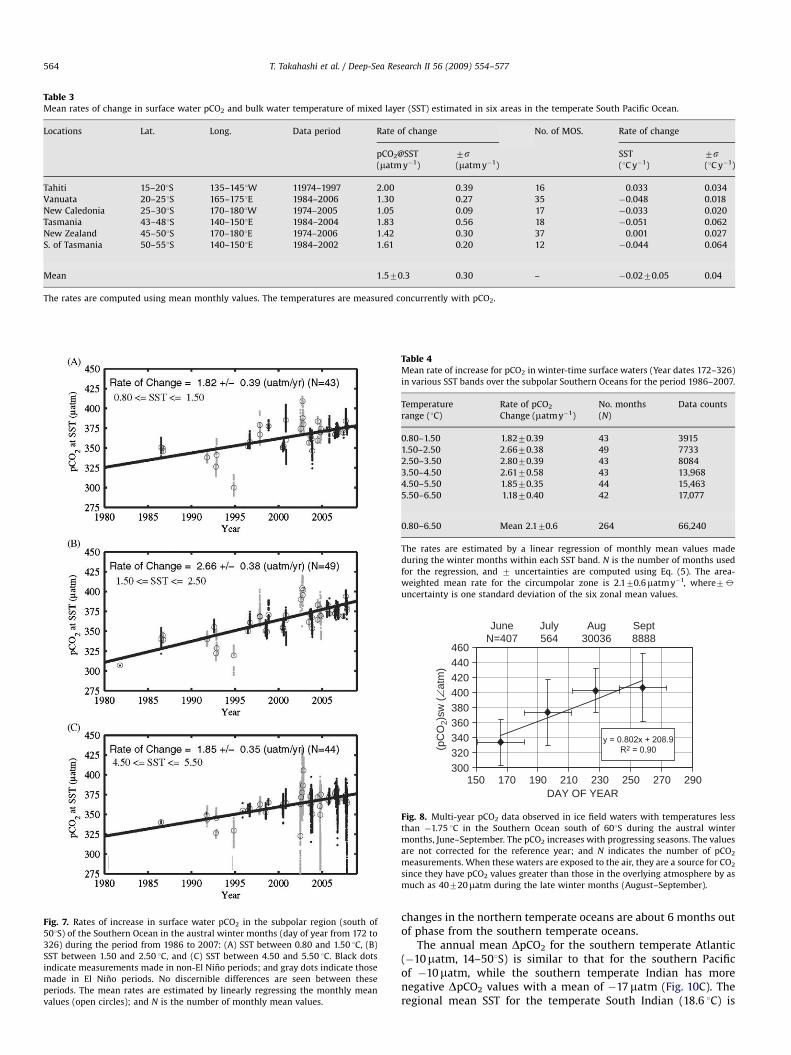
Table 3Mean rates of change in surface water pCO2 and bulk water temperature of mixed layer (SST) estimated in six areas in the temperate South Pacific Ocean.

Locations Lat. Long. Data period Rate of change No. of MOS. Rate of change

pCO2@SST 7s SST 7s(matm y�1) (matm y�1) (1C y�1) (1C y�1)

Tahiti 15–201S 135–1451W 11974–1997 2.00 0.39 16 0.033 0.034

Vanuata 20–251S 165–1751E 1984–2006 1.30 0.27 35 �0.048 0.018

New Caledonia 25–301S 170–1801W 1974–2005 1.05 0.09 17 �0.033 0.020

Tasmania 43–481S 140–1501E 1984–2004 1.83 0.56 18 �0.051 0.062

New Zealand 45–501S 170–1801E 1974–2006 1.42 0.30 37 0.001 0.027

S. of Tasmania 50–551S 140–1501E 1984–2002 1.61 0.20 12 �0.044 0.064

Mean 1.570.3 0.30 – �0.0270.05 0.04

The rates are computed using mean monthly values. The temperatures are measured concurrently with pCO2.

Fig. 7. Rates of increase in surface water pCO2 in the subpolar region (south of

501S) of the Southern Ocean in the austral winter months (day of year from 172 to

326) during the period from 1986 to 2007: (A) SST between 0.80 and 1.50 1C, (B)

SST between 1.50 and 2.50 1C, and (C) SST between 4.50 and 5.50 1C. Black dots

indicate measurements made in non-El Nino periods; and gray dots indicate those

made in El Nino periods. No discernible differences are seen between these

periods. The mean rates are estimated by linearly regressing the monthly mean

values (open circles); and N is the number of monthly mean values.

Table 4Mean rate of increase for pCO2 in winter-time surface waters (Year dates 172–326)

in various SST bands over the subpolar Southern Oceans for the period 1986–2007.

Temperature

range (1C)

Rate of pCO2

Change (matm y�1)

No. months

(N)

Data counts

0.80–1.50 1.8270.39 43 3915

1.50–2.50 2.6670.38 49 7733

2.50–3.50 2.8070.39 43 8084

3.50–4.50 2.6170.58 43 13,968

4.50–5.50 1.8570.35 44 15,463

5.50–6.50 1.1870.40 42 17,077

0.80–6.50 Mean 2.170.6 264 66,240

The rates are estimated by a linear regression of monthly mean values made

during the winter months within each SST band. N is the number of months used

for the regression, and 7 uncertainties are computed using Eq. (5). The area-

weighted mean rate for the circumpolar zone is 2.170.6matm y�1, where7-uncertainty is one standard deviation of the six zonal mean values.

JuneN=407

July564

Aug30036

300320340360380400420440460

150

Sept8888

DAY OF YEAR

(pC

O2)

sw (∠

atm

)

290270250230210190170

Fig. 8. Multi-year pCO2 data observed in ice field waters with temperatures less

than �1.75 1C in the Southern Ocean south of 601S during the austral winter

months, June–September. The pCO2 increases with progressing seasons. The values

are not corrected for the reference year; and N indicates the number of pCO2

measurements. When these waters are exposed to the air, they are a source for CO2

since they have pCO2 values greater than those in the overlying atmosphere by as

much as 40720matm during the late winter months (August–September).

T. Takahashi et al. / Deep-Sea Research II 56 (2009) 554–577564

changes in the northern temperate oceans are about 6 months outof phase from the southern temperate oceans.

The annual mean DpCO2 for the southern temperate Atlantic(�10matm, 14–501S) is similar to that for the southern Pacificof �10matm, while the southern temperate Indian has morenegative DpCO2 values with a mean of �17matm (Fig. 10C). Theregional mean SST for the temperate South Indian (18.6 1C) is

ARTICLE IN PRESS

Table 5Summary of mean rates of increase in surface water pCO2.

No. of box areas Ocean areaa

(106 km2)

Annualb

rate (matm y�1)

Standard deviation

(matm y�1)

References

N. Pacific (10–601N)c 28 28.9 1.28 0.46 Takahashi et al. (2006)

Equatorial Pacific (5–51S)d 2 7.4 1.26 0.55 Feely et al. (2006)

N. Atlantic (15–701N)e 36 16.8 1.80 0.37 This study

S. Pacific (15–551S)e 6 2.9 1.53 0.35 This study

Southern O. (50–601S)f 6 30.6 2.13 0.64 This study

Global with Southern Ocean 78 86.6 (27%) 1.69 0.51

Global without Southern Ocean 72 56.0 (17%) 1.45 0.47

While the rate for the Southern Ocean is estimated for the winter months only, all other rates represent seasonal mean.a Global ocean area ¼ 326.5�106 km2.b Area-weighted mean.c 101(lat.)�101 (long) boxes, excluding the Bering Sea.d Nino 3.4 (120–1701W) and Western Warm Pool (165–1751E) areas.e 51(lat.)�101(long.) boxes.f Winter data only for circumpolar 21 (lat.) wide bands.

T. Takahashi et al. / Deep-Sea Research II 56 (2009) 554–577 565

similar to that for the South Pacific (18.9 1C) and somewhat higherthan the South Atlantic (17.4 1C), and the mean annual surfacewater salinity values are also similar (35.0 for the South Indian,35.4 for the South Atlantic and 35.1 for the South Pacific). Hence,the low pCO2 in the South Indian Ocean cannot be attributed todifferences in SST or salinity. Primary productions estimated fromthe SeaWiFS observations (Gregg et al., 2003) suggest that themean annual productivity in the South Indian is higher than inthe South Pacific, but lower than the South Atlantic. Hence, thebiological production data cannot account for the DpCO2 data. It ispossible that the DpCO2 data and hence the fluxes could be biasedbecause of undersampling in the Southern Hemisphere oceans(see Fig. 1).

A strong negative DpCO2 observed in the spring–summermonths in the sub-arctic Atlantic (Kortzinger et al., 2008) andPacific (Fig. 10A and B) are due to the effect of biologicaldrawdown of CO2, in strongly stratified shallow mixed layers.The seasonal DpCO2 change in subpolar regions is about 4 monthsout of phase from that for the adjacent temperate region.

The positive DpCO2 values observed in July–September in thenorthern Indian Ocean (north of 141N, Fig. 10C) is due to theseasonal upwelling of deep waters caused by the SouthwestMonsoon winds. The positive peak observed in July–October inthe seasonal ice zone of the Southern Ocean (south of 621S,Fig. 10D) represents the under-ice mixed water layer that isenriched with CO2 and nutrients primarily by the vertical mixingof deep waters. During the austral spring–summer months,phytoplankton blooms occurring near ice margins and withinpolynyas reduce DpCO2 values as low as �100matm. However,extent and duration of bloom areas that form a strong sink foratmospheric CO2 may vary geographically and have not been welldocumented.

5.3. Comparison with the 2002 results

Takahashi et al. (2002) used the following procedures forcorrecting the pCO2 data to a reference year 1995. They consideredthat the surface water values in tropical and temperate oceans(451N–501S in the Atlantic, north of 501S in the Indian Oceanand 401N–501S in the western Pacific west of the date line and401N–601S in the eastern Pacific east of the date line) wereincreasing at the same rate as the atmospheric pCO2. As done forthis study, they corrected the observed values to the referenceyear using a mean atmospheric CO2 increase rate of 1.5matm. Onthe other hand, on the basis of a limited number of the pCO2

observations in high latitudes, they considered that CO2 proper-

ties in surface waters in subpolar and polar regions remainedunchanged year to year due to the dilution by vertical mixing ofdeep waters that were little affected by the atmospheric CO2

increase. Accordingly, they made no correction for the time ofpCO2 observations. In contrast, we have demonstrated in thisstudy that the surface water pCO2 over the subpolar oceans hasbeen also increasing at a mean rate of 1.5matm y�1 (rangingbetween 1.3 and 2.0, see Table 5), and used this mean rate fornormalizing the multi-year data to a reference year of 2000 for theentire oceanic areas with the exception of the Bering Sea, wherethe observed rate of �1.2matm y�1 is used.

The difference maps between the surface water pCO2 valuesfrom this study (3.0 M) and the 2002 study (0.94 M) are shown inFig. 11: (A) February and (B) August. To make these two studiescomparable, the 2002 values, which were normalized to areference year 1995, are corrected by adding 7.5matm ( ¼ 1.5matm y�1

�5 y) to adjust them to the reference year 2000.Reflecting the assumptions made in the 2002 study, largerdifferences are found in the subpolar to polar regions. Differencesin the temperate and tropical areas are less than 5matm on theaverage. In the seasonal ice zone of the Southern Ocean south ofabout 621S, the results of this study are found as much as100matm greater than those of 2002 (Fig. 11B). This is attributedto the high pCO2 values revealed by new measurements for under-ice waters during austral winter (Fig. 8). In the Arctic Chukchi Sea,the values for this study are found to be lower than those for the2002 study by as much as 100matm both in February and August.Although this is attributed to new measurements, the time–spacecoverage of the Arctic waters is highly limited presently.

6. Net sea–air CO2 flux

6.1. Computational method

The net sea–air CO2 flux (F) is estimated using

F ¼ kaDpCO2 ¼ TrDpCO2 (7)

where k is the CO2 gas transfer velocity; a is the solubility of CO2

in seawater; Tr is the sea–air gas transfer coefficient; and DpCO2 isthe sea–air pCO2 difference in the reference year 2000 as definedby Eq. (4). The gas transfer velocity (k) is typically expressed as apower function of wind speed (U): kpUn at a given temperatureand salinity. The value of exponent, n, has been suggested tobe between 1 (Liss and Merlivat, 1986) and 3 (Wanninkhof andMcGillis, 1999). Ho et al. (2006), on the basis of the 3He/SF6 doubletracer data obtained over high wind speed conditions (up to

ARTICLE IN PRESS

Fig. 9. The monthly mean values for sea–air pCO2 differences in the global ocean. The values represent climatological mean for non-El Nino conditions adjusted to a reference

year 2000. Orange–yellow colors indicate positive DpCO2 (sea is a source for atmospheric CO2), green indicates near zero DpCO2, and cyan–blue colors indicate negative DpCO2

(sea is a CO2 sink). Heavy pink curves indicate the mean position for the northerly extent of 90% ice cover. Waters under the Southern Ocean ice-field have high positive DpCO2.

Whenever measurements are lacking for ice field waters, the values are estimated using the equation in Fig. 8. (For interpretation of the references to color in this figure legend,

the reader is referred to the web version of this article.).

T. Takahashi et al. / Deep-Sea Research II 56 (2009) 554–577566

ARTICLE IN PRESS

-60

-40

-20

0

20

40

60

1MONTH

N of 50N 14N-50N14N-14S 14S-50S

N of 50N 14N-50N14N-14S 14S-50S

N of14N 14N-14S14S-50S

50S-62SS of 62SGLOBAL MEAN

1312111098765432

ΔpC

O2

(μat

m)

-60

-40

-20

0

20

40

60

1MONTH

1312111098765432

ΔpC

O2

(μat

m)

-60

-40

-20

0

20

40

60

1MONTH

1312111098765432

ΔpC

O2

(μat

m)

-60

-40

-20

0

20

40

60

1MONTH

1312111098765432

ΔpC

O2

(μat

m)

(C) (D)

(A) (B)

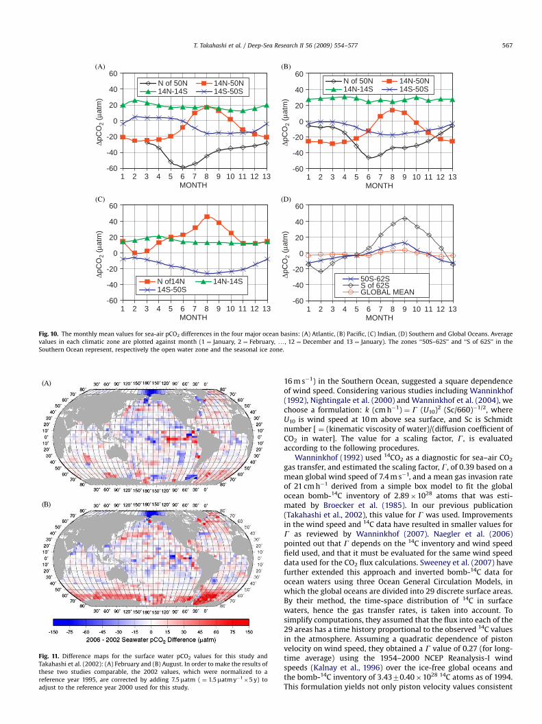
Fig. 10. The monthly mean values for sea-air pCO2 differences in the four major ocean basins: (A) Atlantic, (B) Pacific, (C) Indian, (D) Southern and Global Oceans. Average

values in each climatic zone are plotted against month (1 ¼ January, 2 ¼ February, y, 12 ¼ December and 13 ¼ January). The zones ‘‘50S–62S’’ and ‘‘S of 62S’’ in the

Southern Ocean represent, respectively the open water zone and the seasonal ice zone.

Fig. 11. Difference maps for the surface water pCO2 values for this study and

Takahashi et al. (2002): (A) February and (B) August. In order to make the results of

these two studies comparable, the 2002 values, which were normalized to a

reference year 1995, are corrected by adding 7.5matm ( ¼ 1.5matm y�1�5 y) to

adjust to the reference year 2000 used for this study.

T. Takahashi et al. / Deep-Sea Research II 56 (2009) 554–577 567

16 m s�1) in the Southern Ocean, suggested a square dependenceof wind speed. Considering various studies including Wanninkhof(1992), Nightingale et al. (2000) and Wanninkhof et al. (2004), wechoose a formulation: k (cm h�1) ¼ G (U10)2 (Sc/660)�1/2, whereU10 is wind speed at 10 m above sea surface, and Sc is Schmidtnumber [ ¼ (kinematic viscosity of water)/(diffusion coefficient ofCO2 in water]. The value for a scaling factor, G, is evaluatedaccording to the following procedures.

Wanninkhof (1992) used 14CO2 as a diagnostic for sea–air CO2

gas transfer, and estimated the scaling factor, G, of 0.39 based on amean global wind speed of 7.4 m s�1, and a mean gas invasion rateof 21 cm h�1 derived from a simple box model to fit the globalocean bomb-14C inventory of 2.89�1028 atoms that was esti-mated by Broecker et al. (1985). In our previous publication(Takahashi et al., 2002), this value for G was used. Improvementsin the wind speed and 14C data have resulted in smaller values forG as reviewed by Wanninkhof (2007). Naegler et al. (2006)pointed out that G depends on the 14C inventory and wind speedfield used, and that it must be evaluated for the same wind speeddata used for the CO2 flux calculations. Sweeney et al. (2007) havefurther extended this approach and inverted bomb-14C data forocean waters using three Ocean General Circulation Models, inwhich the global oceans are divided into 29 discrete surface areas.By their method, the time-space distribution of 14C in surfacewaters, hence the gas transfer rates, is taken into account. Tosimplify computations, they assumed that the flux into each of the29 areas has a time history proportional to the observed 14C valuesin the atmosphere. Assuming a quadratic dependence of pistonvelocity on wind speed, they obtained a G value of 0.27 (for long-time average) using the 1954–2000 NCEP Reanalysis-I windspeeds (Kalnay et al., 1996) over the ice-free global oceans andthe bomb-14C inventory of 3.4370.40�1028 14C atoms as of 1994.This formulation yields not only piston velocity values consistent

ARTICLE IN PRESS

T. Takahashi et al. / Deep-Sea Research II 56 (2009) 554–577568

with those obtained from some small-scale deliberate tracerstudies (e.g. Nightingale et al., 2000), but also with the totalbomb-14C inventory obtained for the strato- and troposphere.

For this study, a G value of 0.26 has been computed using the1979–2005 NCEP-DOE AMIP-II Reanalysis 6-h wind speed data(Kanamitsu et al., 2002), which is recast onto the same 41�51 gridas used for this study. The value includes the effect of dilutionof ocean water 14CO2 by the uptake of fossil fuel CO2 (free of 14C).The wind speed data have a mean speed /U10S of 8.06 m s�1 and/U10

2 S//U10S2 of 1.20 for ice-free oceans using the 6-h wind to

calculate /U102 S. The overall error in G is estimated to be 730%

that includes uncertainties in the 14C inventory, ocean models andp14CO2 (Sweeney et al., 2007).

6.2. Distribution of the sea–air CO2 gas transfer coefficient

The product of the first two terms in Eq. (7) represents asea–air CO2 gas transfer rate constant (hereafter called gastransfer coefficient). When monthly mean wind speeds (U10 inthe unit of meters s�1) and a in (mol liter�1 atm�1) (Weiss, 1974)are used, Eq. (8) gives the transfer coefficient (Tr):

Trðg� C m�2 month�1 matm�1Þ ¼ 0:585 � a � ðScÞ�1=2� ðU10Þ

2 (8)

where 0.585 is a unit conversion factor taking into account thescaling factor for the gas transfer rate (0.26), (mol liter�1 atm�1) to(g-C m�3matm�1), (cm h�1 ) to (m month�1) ( ¼ 10�2

�24�365/12),and a reference Schmidt number (6601/2). The Schmidt number(Sc) and the solubility of CO2 in seawater depend sensitively on

0.00

0.02

0.04

0.06

0.08

0.10

0.12

0.14

1MONTH

N of 50N50N-14N14N-14S14S-50S

1312111098765432

TRA

NS

F. C

OE

FF.

(gm

-C m

o-1

m-2

μat

m-1

)

N of 14N 14N-14S14S-50S

0.00

0.02

0.04

0.06

0.08

0.10

0.12

0.14

1MONTH

1312111098765432

TRA

NS

F. C

OE

FF.

(gm

-C m

o-1

m-2

μat

m-1

)

(A)

(C)

Fig. 12. Monthly mean values for the CO2 gas transfer rate coefficient, Tr, in (g-carbon m

each 41�51 box were computed using the 1979–2005 NCEP-DOE AMIP-II Reanalysis da

zone shown in the plots are area-weighted mean values of the box areas within each

13 ¼ January.

the temperature: from 01 to 30 1C, Sc for CO2 decreases by a factorof 5 and a also decreases by a factor of 2.5. Accordingly, theproduct a � (Sc)�1/2 is nearly constant and changes by less than 10%over the temperature range of global surface ocean waters. Hence,the transfer rate coefficient, Tr, is primarily a function of windspeed. Since a product of Tr with DpCO2 gives the net sea–air CO2

flux, the seasonal and geographical variation of Tr is of interest.In Fig. 12, the monthly mean Tr values in six climatic zones are

summarized for the four major ocean basins and the global ocean.The subpolar regions of the North Atlantic (Fig. 12A, northof 501N) and the Southern Ocean (Fig. 12D, 50–21S) have thehighest values for the transfer rate coefficient reaching as high as0.12 g-C m�2 month�1matm�1 (hereafter the unit is omitted) dueto persistent high winds during the regions’ respective wintermonths. During the summer months, however, the Tr valuesdecrease to as low as 0.03 in the sub-arctic Atlantic (Fig. 12A) andto 0.08 in the Southern Ocean (Fig. 12D). In contrast, winter-maximum Tr values reach only to 0.09 in the sub-arctic Pacific.The Antarctic zone (south of 621S, Fig. 12D) has much lower windspeeds and hence shows lower Tr values ranging between 0.07 inwinter and 0.05 in summer. In the temperate zones of the Atlanticand Pacific, the Tr values vary from summer values of about 0.03to winter values of 0.07 (Fig. 12A and B); and the seasonal changesin the northern oceans are 6 months out of phase from theSouthern Hemisphere oceans. The tropical Atlantic and Pacific(Fig. 12A and B, 141N–141S) have Tr values of about 0.03, and showvery small seasonal variability. The northern Indian Ocean issignificantly different from the Atlantic and Pacific. Tr values peakin June–August due to southwest monsoon winds in the tropical

N of 50N 50N-14N14N-14S 14S-50S

0.00

0.02

0.04

0.06

0.08

0.10

0.12

0.14

1MONTH

1312111098765432

TRA

NS

F. C

OE

FF.

(gm

-C m

o-1

m-2

μat

m-1

)

50S-62S S of 62SGLOBAL

0.00

0.02

0.04

0.06

0.08

0.10

0.12

0.14

1MONTH

1312111098765432

TRA

NS

F. C

OE

FF.

(gm

-C m

o-1

m-2

μat

m-1

)

(B)

(D)

�2 month�1matm�1) computed using Eq. (8). The monthly mean values for U10 in

ta (updated version of Kanamitsu et al., 2002). The monthly mean values for each

zone. Months are expressed as 1 ¼ January, 2 ¼ February,y, 12 ¼ December and

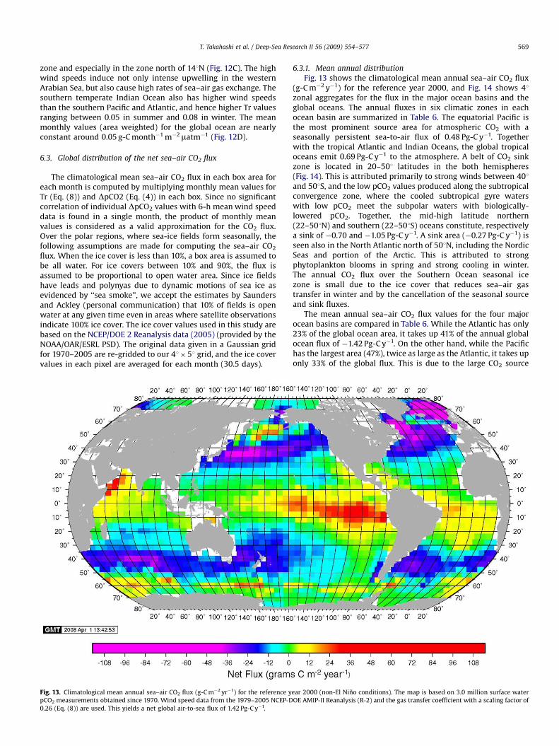
ARTICLE IN PRESS

T. Takahashi et al. / Deep-Sea Research II 56 (2009) 554–577 569

zone and especially in the zone north of 141N (Fig. 12C). The highwind speeds induce not only intense upwelling in the westernArabian Sea, but also cause high rates of sea–air gas exchange. Thesouthern temperate Indian Ocean also has higher wind speedsthan the southern Pacific and Atlantic, and hence higher Tr valuesranging between 0.05 in summer and 0.08 in winter. The meanmonthly values (area weighted) for the global ocean are nearlyconstant around 0.05 g-C month�1 m�2matm�1 (Fig. 12D).

6.3. Global distribution of the net sea–air CO2 flux

The climatological mean sea–air CO2 flux in each box area foreach month is computed by multiplying monthly mean values forTr (Eq. (8)) and DpCO2 (Eq. (4)) in each box. Since no significantcorrelation of individual DpCO2 values with 6-h mean wind speeddata is found in a single month, the product of monthly meanvalues is considered as a valid approximation for the CO2 flux.Over the polar regions, where sea-ice fields form seasonally, thefollowing assumptions are made for computing the sea–air CO2

flux. When the ice cover is less than 10%, a box area is assumed tobe all water. For ice covers between 10% and 90%, the flux isassumed to be proportional to open water area. Since ice fieldshave leads and polynyas due to dynamic motions of sea ice asevidenced by ‘‘sea smoke’’, we accept the estimates by Saundersand Ackley (personal communication) that 10% of fields is openwater at any given time even in areas where satellite observationsindicate 100% ice cover. The ice cover values used in this study arebased on the NCEP/DOE 2 Reanalysis data (2005) (provided by theNOAA/OAR/ESRL PSD). The original data given in a Gaussian gridfor 1970–2005 are re-gridded to our 41�51 grid, and the ice covervalues in each pixel are averaged for each month (30.5 days).

Fig. 13. Climatological mean annual sea–air CO2 flux (g-C m�2 yr�1) for the reference y

pCO2 measurements obtained since 1970. Wind speed data from the 1979–2005 NCEP-D

0.26 (Eq. (8)) are used. This yields a net global air-to-sea flux of 1.42 Pg-C y�1.

6.3.1. Mean annual distribution

Fig. 13 shows the climatological mean annual sea–air CO2 flux(g-C m�2 y�1) for the reference year 2000, and Fig. 14 shows 41zonal aggregates for the flux in the major ocean basins and theglobal oceans. The annual fluxes in six climatic zones in eachocean basin are summarized in Table 6. The equatorial Pacific isthe most prominent source area for atmospheric CO2 with aseasonally persistent sea-to-air flux of 0.48 Pg-C y�1. Togetherwith the tropical Atlantic and Indian Oceans, the global tropicaloceans emit 0.69 Pg-C y�1 to the atmosphere. A belt of CO2 sinkzone is located in 20–501 latitudes in the both hemispheres(Fig. 14). This is attributed primarily to strong winds between 401and 501S, and the low pCO2 values produced along the subtropicalconvergence zone, where the cooled subtropical gyre waterswith low pCO2 meet the subpolar waters with biologically-lowered pCO2. Together, the mid-high latitude northern(22–501N) and southern (22–501S) oceans constitute, respectivelya sink of �0.70 and �1.05 Pg-C y�1. A sink area (�0.27 Pg-C y�1) isseen also in the North Atlantic north of 501N, including the NordicSeas and portion of the Arctic. This is attributed to strongphytoplankton blooms in spring and strong cooling in winter.The annual CO2 flux over the Southern Ocean seasonal icezone is small due to the ice cover that reduces sea–air gastransfer in winter and by the cancellation of the seasonal sourceand sink fluxes.

The mean annual sea–air CO2 flux values for the four majorocean basins are compared in Table 6. While the Atlantic has only23% of the global ocean area, it takes up 41% of the annual globalocean flux of �1.42 Pg-C y�1. On the other hand, while the Pacifichas the largest area (47%), twice as large as the Atlantic, it takes uponly 33% of the global flux. This is due to the large CO2 source

ear 2000 (non-El Nino conditions). The map is based on 3.0 million surface water

OE AMIP-II Reanalysis (R-2) and the gas transfer coefficient with a scaling factor of

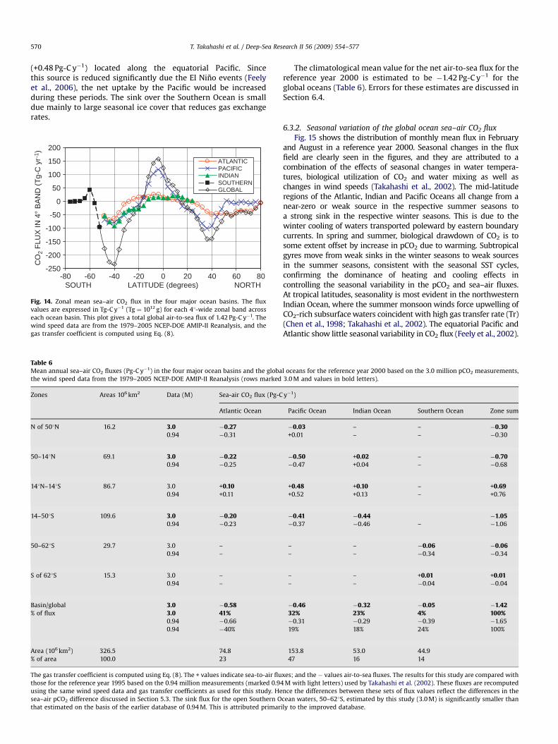
ARTICLE IN PRESS

T. Takahashi et al. / Deep-Sea Research II 56 (2009) 554–577570

(+0.48 Pg-C y�1) located along the equatorial Pacific. Sincethis source is reduced significantly due the El Nino events (Feelyet al., 2006), the net uptake by the Pacific would be increasedduring these periods. The sink over the Southern Ocean is smalldue mainly to large seasonal ice cover that reduces gas exchangerates.

-250

-200

-150

-100

-50

0

50

100

150

200

-80LATITUDE (degrees)

ATLANTICPACIFICINDIANSOUTHERNGLOBAL

CO

2 FL

UX

IN 4

° B

AN

D (T

g-C

yr-1

)

NORTHSOUTH806040200-20-40-60

Fig. 14. Zonal mean sea–air CO2 flux in the four major ocean basins. The flux

values are expressed in Tg-C y�1 (Tg ¼ 1012 g) for each 41-wide zonal band across

each ocean basin. This plot gives a total global air-to-sea flux of 1.42 Pg-C y�1. The

wind speed data are from the 1979–2005 NCEP-DOE AMIP-II Reanalysis, and the

gas transfer coefficient is computed using Eq. (8).

Table 6Mean annual sea–air CO2 fluxes (Pg-C y�1) in the four major ocean basins and the globa

the wind speed data from the 1979–2005 NCEP-DOE AMIP-II Reanalysis (rows marked

Zones Areas 106 km2 Data (M) Sea-air CO2 flux (Pg-C

Atlantic Ocean

N of 501N 16.2 3.0 �0.270.94 �0.31

50–141N 69.1 3.0 �0.220.94 �0.25

141N–141S 86.7 3.0 +0.100.94 +0.11

14–501S 109.6 3.0 �0.200.94 �0.23

50–621S 29.7 3.0 –

0.94 –

S of 621S 15.3 3.0 –

0.94 –

Basin/global 3.0 �0.58% of flux 3.0 41%

0.94 �0.66

0.94 �40%

Area (106 km2) 326.5 74.8

% of area 100.0 23

The gas transfer coefficient is computed using Eq. (8). The + values indicate sea-to-air flu

those for the reference year 1995 based on the 0.94 million measurements (marked 0.94

using the same wind speed data and gas transfer coefficients as used for this study. He

sea–air pCO2 difference discussed in Section 5.3. The sink flux for the open Southern O

that estimated on the basis of the earlier database of 0.94 M. This is attributed primar

The climatological mean value for the net air-to-sea flux for thereference year 2000 is estimated to be �1.42 Pg-C y�1 for theglobal oceans (Table 6). Errors for these estimates are discussed inSection 6.4.

6.3.2. Seasonal variation of the global ocean sea–air CO2 flux

Fig. 15 shows the distribution of monthly mean flux in Februaryand August in a reference year 2000. Seasonal changes in the fluxfield are clearly seen in the figures, and they are attributed to acombination of the effects of seasonal changes in water tempera-tures, biological utilization of CO2 and water mixing as well aschanges in wind speeds (Takahashi et al., 2002). The mid-latituderegions of the Atlantic, Indian and Pacific Oceans all change from anear-zero or weak source in the respective summer seasons toa strong sink in the respective winter seasons. This is due to thewinter cooling of waters transported poleward by eastern boundarycurrents. In spring and summer, biological drawdown of CO2 is tosome extent offset by increase in pCO2 due to warming. Subtropicalgyres move from weak sinks in the winter seasons to weak sourcesin the summer seasons, consistent with the seasonal SST cycles,confirming the dominance of heating and cooling effects incontrolling the seasonal variability in the pCO2 and sea–air fluxes.At tropical latitudes, seasonality is most evident in the northwesternIndian Ocean, where the summer monsoon winds force upwelling ofCO2-rich subsurface waters coincident with high gas transfer rate (Tr)(Chen et al., 1998; Takahashi et al., 2002). The equatorial Pacific andAtlantic show little seasonal variability in CO2 flux (Feely et al., 2002).

l oceans for the reference year 2000 based on the 3.0 million pCO2 measurements,

3.0 M and values in bold letters).

y�1)

Pacific Ocean Indian Ocean Southern Ocean Zone sum

�0.03 – – �0.30+0.01 – – �0.30

�0.50 +0.02 – �0.70�0.47 +0.04 – �0.68

+0.48 +0.10 – +0.69+0.52 +0.13 – +0.76

�0.41 �0.44 �1.05�0.37 �0.46 – �1.06

– – �0.06 �0.06– – �0.34 �0.34

– – +0.01 +0.01– – �0.04 �0.04

�0.46 �0.32 �0.05 �1.4232% 23% 4% 100%�0.31 �0.29 �0.39 �1.65

19% 18% 24% 100%

153.8 53.0 44.9

47 16 14

xes; and the � values air-to-sea fluxes. The results for this study are compared with

M with light letters) used by Takahashi et al. (2002). These fluxes are recomputed

nce the differences between these sets of flux values reflect the differences in the

cean waters, 50–621S, estimated by this study (3.0 M) is significantly smaller than

ily to the improved database.

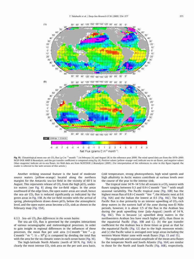
ARTICLE IN PRESS

Fig. 15. Climatological mean sea–air CO2 flux (g-C m�2 month�1) in February (A) and August (B) in the reference year 2000. The wind speed data are from the 1979–2005

NCEP-DOE AMIP-II Reanalysis, and the gas transfer coefficient is computed using Eq. (8). Positive values (yellow–orange–red) indicate sea-to-air fluxes, and negative values

(blue–magenta) indicate air-to-sea fluxes. Ice field data are from NCEP/DOE 2 Reanalysis (2005). (For interpretation of the references to color in this figure legend, the

reader is referred to the web version of this article.).

T. Takahashi et al. / Deep-Sea Research II 56 (2009) 554–577 571

Another striking seasonal feature is the band of moderatesource waters (yellow–orange) located along the northernmargins for the Antarctic sea-ice field in the vicinity of 601S inAugust. This represents release of CO2 from the high pCO2 under-ice waters (see Fig. 8) along the ice-field edges. In the areassouthward of the edge lines, the open water areas are small, hencethe sea–air CO2 flux is reduced significantly as indicated by thegreen areas in Fig. 15B. As the ice field recedes with the arrival ofspring, photosynthesis draws down pCO2 below the atmosphericlevel, and the open water areas become a CO2 sink as shown in theFebruary map (Fig. 15A).

6.3.3. Sea–air CO2 flux differences in the ocean basins

The sea–air CO2 flux is governed by the complex interactionsof various oceanographic and meteorological processes. In orderto gain insight in regional differences in the influences of theseprocesses, the mean flux per unit area (t-C month�1 km�2

¼ g-C month�1 m�2; 1t ¼ 106 g) is computed by dividing the total fluxwith the area for the six climatic zones in each ocean basin (Fig. 16).

The high-latitude North Atlantic (north of 501N, Fig. 16A) isclearly the most intense CO2 sink area on the per unit area basis.

Cold temperature, strong photosynthesis, high wind speeds andhigh alkalinity in Arctic waters contribute at various levels overthe course of the year to the intense sink.

The tropical zone 141N–141S for all oceans is a CO2 source withfluxes ranging between 0.3 and 0.9 t-C month�1 km�2 with smallseasonal variability. The Pacific tropical zone (Fig. 16B) has thehighest mean flux of 0.8 t-C month�1 km�2, the Atlantic next at 0.6(Fig. 16A) and the Indian the lowest at 0.5 (Fig. 16C). The highPacific flux is due primarily to an intense upwelling of CO2-richdeep waters in the eastern half of the zone during non-El Ninoperiods, however, it is about 1/5 of the flux in the Arabian Seaduring the peak upwelling time (July–August) (north of 141N,Fig. 16C). This is because (a) upwelled deep waters in thenorthwestern Arabian Sea have much higher pCO2 than those inthe equatorial Pacific (Figs. 10B and C); (b) the gas transfercoefficient for the Arabian Sea is three times as great as that forthe equatorial Pacific (Fig. 12) due to the high monsoon winds;and (c) the Pacific value is averaged over large areas including thewestern Warm Water zone with weak fluxes (Figs. 13 and 15).

The magnitude and seasonal amplitude of the mean area fluxesfor the temperate North and South Atlantic (Fig. 16A) are similarto those for the North and South Pacific (Fig. 16B), respectively.

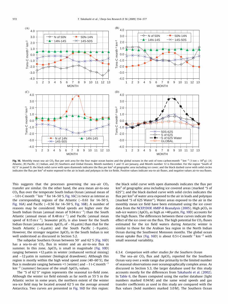
ARTICLE IN PRESS

-4.0

-3.0

-2.0

-1.0

0.0

1.0

2.0

3.0

4.0

1MONTH

N of 50N 50N-14N14N-14S 14S-50S

1312111098765432

Tons

-C m

onth

-1 k

m-2

(A)

N of 50N 50N-14N14N-14S 14S-50S

-4.0

-3.0

-2.0

-1.0

0.0

1.0

2.0

3.0

4.0

1MONTH

1312111098765432

Tons

-C m

onth

-1 k

m-2

(B)

N of 14N 14N-14S14S-50S

-4.0

-3.0

-2.0

-1.0

0.0

1.0

2.0

3.0

4.0

1MONTH

1312111098765432

Tons

-C m

onth

-1 k

m-2

(C)

50S-62SS of 62SS of 62S WaterGLOBAL

-4.0

-3.0

-2.0

-1.0

0.0

1.0

2.0

3.0

4.0

1MONTH

1312111098765432

Tons

-C m

onth

-1 k

m-2

(D)

Fig. 16. Monthly mean sea–air CO2 flux per unit area for the four major ocean basins and the global oceans in the unit of tons-carbon month�1 km�2 (1 ton ¼ 106 g): (A)

Atlantic, (B) Pacific, (C) Indian, and (D) Southern and Global Oceans. Month numbers 1 and 13 are January, and Month number 12 is December. For the region ‘‘South of

621S’’ in panel D, the black solid curve with open diamonds indicates the flux per km2 of geographic area including ice cover; and the black dashed curve with solid circles

indicates the flux per km2 of water exposed to the air in leads and polynyas in the ice fields. Positive values indicate sea-to-air fluxes, and negative values air-to-sea fluxes.

T. Takahashi et al. / Deep-Sea Research II 56 (2009) 554–577572

This suggests that the processes governing the sea–air CO2

transfer are similar. On the other hand, the area mean air-to-seaCO2 flux over the temperate South Indian Ocean (annual mean of�1.0 t-C month�1 km�2 for 14–501S, Fig. 16C) is twice as intense asthe corresponding regions of the Atlantic (�0.61 for 14–501S,Fig. 16A) and Pacific (�0.56 for 14–501S, Fig. 16B). A number ofreasons may be considered. Wind speeds are higher over theSouth Indian Ocean (annual mean of 9.04 m s�1) than the SouthAtlantic (annual mean of 8.48 m s�1) and Pacific (annual meanspeed of 8.15 m s�1). Seawater pCO2 is also lower for the SouthIndian Ocean (annual mean DpCO2 of �16matm) than that for theSouth Atlantic (�6matm) and the South Pacific (�9matm).However, the stronger negative DpCO2 in the South Indian is notwell understood as discussed in Section 5.2.

The subpolar Southern Ocean between 501 and 621S (Fig. 16D)has a sea-to-air CO2 flux in winter and an air-to-sea flux insummer. In this zone, DpCO2 is small in magnitude (Fig. 10D)ranging between +12matm in winter (enhanced vertical mixing)and �12matm in summer (biological drawdown). Although thisregion is mostly within the high wind speed zone (40–601S), theflux is moderate ranging between +1 (winter) and �1 t-C month�1

km�2 (summer) because of the small DpCO2 values.The ‘‘S of 621S’’ region represents the seasonal ice-field zone.

Although the winter ice field extends as far north as 551S in theAtlantic sector in some years, the northern extent of the wintersea-ice field may be located around 621S on the average aroundAntarctica. Two curves are presented in Fig. 16D for this region:

the black solid curve with open diamonds indicates the flux perkm2 of geographic area including ice covered areas (marked ‘‘S of62S’’); and the black dashed curve with solid circles indicates theflux per km2 of water area exposed to the air in leads and polynyas(marked ‘‘S of 62S Water’’). Water areas exposed to the air in themonthly mean ice field have been estimated using the ice coverdata from the NCEP/DOE AMIP-II Reanalysis (2005). High pCO2 insub-ice waters (DpCO2 as high as +40matm, Fig. 10D) accounts forthe high fluxes. The differences between these curves indicate theeffect of the ice cover on the flux. The high potential for CO2 fluxesestimated for the ice field waters during Antarctic winter issimilar to those for the Arabian Sea region in the North IndianOcean during the Southwest Monsoon months. The global oceanmean uptake flux (Fig. 16D) is about 0.5 t-C month�1 km�2 withsmall seasonal variability.

6.3.4. Comparison with other studies for the Southern Ocean

The sea–air CO2 flux and DpCO2 reported for the SouthernOcean vary over a wide range due primarily to the limited numberof seasonal observations over oceanographically complex areas. Asdiscussed in Section 5.3, the larger database used for this studyaccounts mostly for the differences from Takahashi et al. (2002).In Table 6, the fluxes computed using the earlier database (lightnumbers marked 0.94 M) and the same wind speeds and gastransfer coefficients as used in this study are compared with theflux values (bold numbers marked 3.0 M). The Southern Ocean

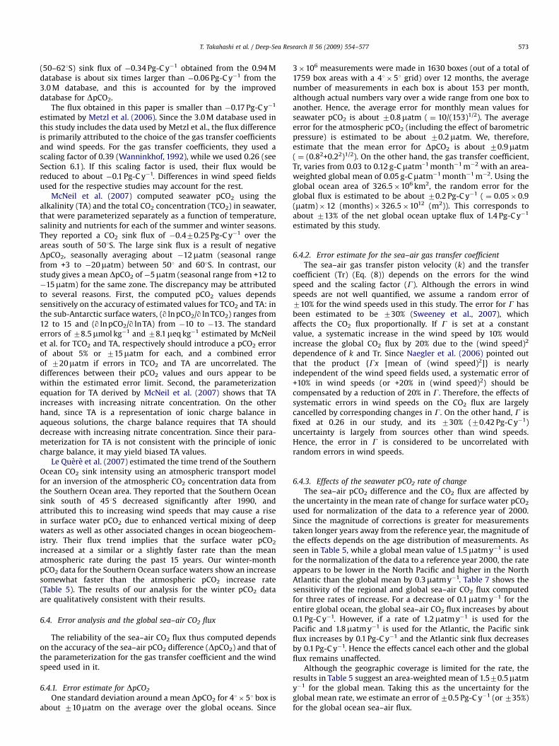
ARTICLE IN PRESS

T. Takahashi et al. / Deep-Sea Research II 56 (2009) 554–577 573

(50–621S) sink flux of �0.34 Pg-C y�1 obtained from the 0.94 Mdatabase is about six times larger than �0.06 Pg-C y�1 from the3.0 M database, and this is accounted for by the improveddatabase for DpCO2.

The flux obtained in this paper is smaller than �0.17 Pg-C y�1

estimated by Metzl et al. (2006). Since the 3.0 M database used inthis study includes the data used by Metzl et al., the flux differenceis primarily attributed to the choice of the gas transfer coefficientsand wind speeds. For the gas transfer coefficients, they used ascaling factor of 0.39 (Wanninkhof, 1992), while we used 0.26 (seeSection 6.1). If this scaling factor is used, their flux would bereduced to about �0.1 Pg-C y�1. Differences in wind speed fieldsused for the respective studies may account for the rest.

McNeil et al. (2007) computed seawater pCO2 using thealkalinity (TA) and the total CO2 concentration (TCO2) in seawater,that were parameterized separately as a function of temperature,salinity and nutrients for each of the summer and winter seasons.They reported a CO2 sink flux of �0.470.25 Pg-C y�1 over theareas south of 501S. The large sink flux is a result of negativeDpCO2, seasonally averaging about �12matm (seasonal rangefrom +3 to �20matm) between 501 and 601S. In contrast, ourstudy gives a mean DpCO2 of �5matm (seasonal range from +12 to�15matm) for the same zone. The discrepancy may be attributedto several reasons. First, the computed pCO2 values dependssensitively on the accuracy of estimated values for TCO2 and TA: inthe sub-Antarctic surface waters, (q ln pCO2/q ln TCO2) ranges from12 to 15 and (q ln pCO2/q ln TA) from �10 to �13. The standarderrors of 78.5mmol kg�1 and 78.1meq kg�1 estimated by McNeilet al. for TCO2 and TA, respectively should introduce a pCO2 errorof about 5% or 715matm for each, and a combined errorof 720matm if errors in TCO2 and TA are uncorrelated. Thedifferences between their pCO2 values and ours appear to bewithin the estimated error limit. Second, the parameterizationequation for TA derived by McNeil et al. (2007) shows that TAincreases with increasing nitrate concentration. On the otherhand, since TA is a representation of ionic charge balance inaqueous solutions, the charge balance requires that TA shoulddecrease with increasing nitrate concentration. Since their para-meterization for TA is not consistent with the principle of ioniccharge balance, it may yield biased TA values.

Le Quere et al. (2007) estimated the time trend of the SouthernOcean CO2 sink intensity using an atmospheric transport modelfor an inversion of the atmospheric CO2 concentration data fromthe Southern Ocean area. They reported that the Southern Oceansink south of 451S decreased significantly after 1990, andattributed this to increasing wind speeds that may cause a risein surface water pCO2 due to enhanced vertical mixing of deepwaters as well as other associated changes in ocean biogeochem-istry. Their flux trend implies that the surface water pCO2

increased at a similar or a slightly faster rate than the meanatmospheric rate during the past 15 years. Our winter-monthpCO2 data for the Southern Ocean surface waters show an increasesomewhat faster than the atmospheric pCO2 increase rate(Table 5). The results of our analysis for the winter pCO2 dataare qualitatively consistent with their results.

6.4. Error analysis and the global sea–air CO2 flux

The reliability of the sea–air CO2 flux thus computed dependson the accuracy of the sea–air pCO2 difference (DpCO2) and that ofthe parameterization for the gas transfer coefficient and the windspeed used in it.

6.4.1. Error estimate for DpCO2

One standard deviation around a mean DpCO2 for 41�51 box isabout 710matm on the average over the global oceans. Since

3�106 measurements were made in 1630 boxes (out of a total of1759 box areas with a 41�51 grid) over 12 months, the averagenumber of measurements in each box is about 153 per month,although actual numbers vary over a wide range from one box toanother. Hence, the average error for monthly mean values forseawater pCO2 is about 70.8matm ( ¼ 10/(153)1/2). The averageerror for the atmospheric pCO2 (including the effect of barometricpressure) is estimated to be about 70.2matm. We, therefore,estimate that the mean error for DpCO2 is about 70.9matm( ¼ (0.82+0.22)1/2). On the other hand, the gas transfer coefficient,Tr, varies from 0.03 to 0.12 g-Cmatm–1 month�1 m�2 with an area-weighted global mean of 0.05 g-Cmatm�1 month�1 m�2. Using theglobal ocean area of 326.5�106 km2, the random error for theglobal flux is estimated to be about 70.2 Pg-C y�1 ( ¼ 0.05�0.9(matm)�12 (months)�326.5�1012 (m2)). This corresponds toabout 713% of the net global ocean uptake flux of 1.4 Pg-C y�1

estimated by this study.

6.4.2. Error estimate for the sea–air gas transfer coefficient

The sea–air gas transfer piston velocity (k) and the transfercoefficient (Tr) (Eq. (8)) depends on the errors for the windspeed and the scaling factor (G). Although the errors in windspeeds are not well quantified, we assume a random error of710% for the wind speeds used in this study. The error for G hasbeen estimated to be 730% (Sweeney et al., 2007), whichaffects the CO2 flux proportionally. If G is set at a constantvalue, a systematic increase in the wind speed by 10% wouldincrease the global CO2 flux by 20% due to the (wind speed)2

dependence of k and Tr. Since Naegler et al. (2006) pointed outthat the product {Gx [mean of (wind speed)2]} is nearlyindependent of the wind speed fields used, a systematic error of+10% in wind speeds (or +20% in (wind speed)2) should becompensated by a reduction of 20% in G. Therefore, the effects ofsystematic errors in wind speeds on the CO2 flux are largelycancelled by corresponding changes in G. On the other hand, G isfixed at 0.26 in our study, and its 730% (70.42 Pg-C y�1)uncertainty is largely from sources other than wind speeds.Hence, the error in G is considered to be uncorrelated withrandom errors in wind speeds.

6.4.3. Effects of the seawater pCO2 rate of change

The sea–air pCO2 difference and the CO2 flux are affected bythe uncertainty in the mean rate of change for surface water pCO2

used for normalization of the data to a reference year of 2000.Since the magnitude of corrections is greater for measurementstaken longer years away from the reference year, the magnitude ofthe effects depends on the age distribution of measurements. Asseen in Table 5, while a global mean value of 1.5matm y�1 is usedfor the normalization of the data to a reference year 2000, the rateappears to be lower in the North Pacific and higher in the NorthAtlantic than the global mean by 0.3matm y�1. Table 7 shows thesensitivity of the regional and global sea–air CO2 flux computedfor three rates of increase. For a decrease of 0.1matm y�1 for theentire global ocean, the global sea–air CO2 flux increases by about0.1 Pg-C y�1. However, if a rate of 1.2matm y�1 is used for thePacific and 1.8matm y�1 is used for the Atlantic, the Pacific sinkflux increases by 0.1 Pg-C y�1 and the Atlantic sink flux decreasesby 0.1 Pg-C y�1. Hence the effects cancel each other and the globalflux remains unaffected.

Although the geographic coverage is limited for the rate, theresults in Table 5 suggest an area-weighted mean of 1.570.5matmy�1 for the global mean. Taking this as the uncertainty for theglobal mean rate, we estimate an error of 70.5 Pg-C y�1 (or 735%)for the global ocean sea–air flux.

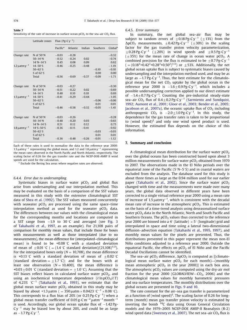
ARTICLE IN PRESS

Table 7Sensitivity of the rate of increase in surface ocean pCO2 to the sea–air CO2 flux.

Latitude zones Flux (Pg-C y�1)

Pacifica Atlantic Indian Southern Globala

Change rate N of 501N �0.03 �0.28 �0.32

50–141N �0.52 �0.24 0.02 �0.74

141N–141S 0.45 0.08 0.09 0.62

1.2matm y�1 14–501S �0.46 �0.25 �0.48 �1.19

50–621S �0.10 �0.10

S of 621S 0.00 0.00

Total �0.56 �0.69 �0.37 �0.09 �1.71

Change rate N of 501N �0.03 �0.27 �0.30

50–141N �0.51 �0.22 0.02 �0.69

14–141S 0.48 0.10 0.10 0.69

1.5matm y�1 14–501S �0.41 �0.29 �0.44 �1.05

50–621S �0.06 �0.06

S of 621S 0.01 0.01

Total �0.46 �0.58 �0.32 �0.05 �1.41

Change rate N of 501N �0.03 �0.26 �0.28

50–141N �0.48 �0.20 0.03 �0.65

141N–141S 0.51 0.12 0.12 0.75

1.8matm y�1 141S–501S �0.36 �0.15 �0.41 �0.92

50–621S �0.03 �0.03

S of 621S 0.01 0.01

Total �0.36 �0.48 �0.26 �0.01 �1.12

Each of these rates is used to normalize the data to the reference year 2000:

1.5matm y�1 representing the global mean, and 1.2 and 1.8matm y�1 representing

the mean rates observed in the North Pacific and North Atlantic, respectively. The

scaling factor of 0.26 for the gas transfer rate and the NCEP-DOE-AMIP II wind

speeds are used for the calculation.a Exclude the Bering Sea areas where negative rates are observed.

T. Takahashi et al. / Deep-Sea Research II 56 (2009) 554–577574

6.4.4. Error due to undersampling

Systematic biases in surface water pCO2 and global fluxarise from undersampling and our interpolation method. Thismay be evaluated on the basis of a comparison of the SST valuesmeasured in this study with the extensive climatological SSTdata of Shea et al. (1992). The SST values measured concurrentlywith seawater pCO2 are processed using the same space–timeinterpolation method as used for the seawater pCO2 data.The differences between our values with the climatological meanfor the corresponding months and locations are computed ina SST range from �1.9 to 30 1C and averaged (see Fig. 3of Takahashi et al., 1997, as an example). For 21,108 pairs ofcomparison for monthly mean values, that include those for boxeswith measurements as well as those interpolated (due to nomeasurements), the mean difference for (interpolated–climatologicalmean) is found to be +0.08 1C with a standard deviationof mean of 70.01 1C ( ¼ (1.4 1C standard deviation)/(21,108)1/2).For the interpolated boxes only (N ¼ 10,708), the mean differenceis +0.13 1C with a standard deviation of mean of 70.02 1C(standard deviation ¼71.7 1C); and for the boxes with atleast one observation (N ¼ 10,400), the mean difference is+0.0370.01 1C (standard deviation ¼71.0 1C). Assuming that theSST biases reflect biases in calculated surface water pCO2, andusing an isochemical temperature dependence (q ln pCO2/qT)of 4.23% 1C�1 (Takahashi et al., 1993), we estimate that theglobal mean surface water pCO2 obtained in this study may bebiased by about +1.3matm ( ¼ 350matm�0.0423 1C�1

�0.08 1C).This corresponds to a flux bias of 20% (or 0.25 Pg-C y�1) when aglobal mean transfer coefficient of 0.05 g-C m�2matm�1 month�1

is used. Accordingly, our global ocean uptake flux of �1.42 Pg-C y�1 may be biased low by about 20%, and could be as largeas �1.7 Pg-C y�1.

6.4.5. Error summary

In summary, the net global sea–air flux may besubject to random errors of 70.18 Pg-C y�1 (713%) from theDpCO2 measurements, 70.42 Pg-C y�1 (730%) in the scalingfactor for the gas transfer piston velocity parameterization,70.28 Pg-C y�1 (720%) in wind speeds and 70.5 Pg-C y�1

(735%) for the mean rate of change in ocean water pCO2. Acombined precision for the flux is estimated to be 70.7 Pg-C y�1

( ¼ (0.182+0.422+0.282+0.502)1/2) or 753%. Additionally, the netglobal ocean uptake flux is subject to systematic biases caused byundersampling and the interpolation method used, and may be aslarge as �1.7 Pg-C y�1. Thus, the best estimate for the climatolo-gical mean for the net CO2 uptake by the global ocean in thereference year 2000 is �1.670.9 Pg-C y�1, which includes apossible undersampling correction applied to our direct estimateof �1.470.7 Pg-C y�1. Counting the pre-industrial steady-statesea–air CO2 flux of 0.470.2 Pg-C y�1 (Sarmiento and Sundquist,1992; Aumont et al., 2001; Gloor et al., 2003; Bender et al., 2005;Jacobson et al., 2007a), the oceanic uptake flux of CO2 includinganthropogenic CO2 is �2.071.0 Pg-C y�1. In this study, thedependence for the gas transfer rates is taken to be proportionalto (wind speed)2 and only one wind speed product is used.However, the estimated flux depends on the choice of thisinformation.

7. Summary and conclusion

A climatological mean distribution for the surface water pCO2

over the global oceans has been constructed based upon about 3million measurements for surface water pCO2 obtained from 1970to 2007. The observations made in the El Nino periods over theequatorial zone of the Pacific (51N–51S) and in coastal waters areexcluded from the analysis. The database used for this study isabout three times as large as the 0.94 million used for our earlierpaper (Takahashi et al., 2002). Since the surface water pCO2

changed with time and the measurements were made over manyyears, the global data observed in different years have beencorrected to a single virtual reference year 2000 using a mean rateof increase of 1.5matm y�1, which is consistent with the decadalmean rate of increase in the atmospheric pCO2. This is estimatedon the basis of a time-trend analysis using deseasonalized surfacewater pCO2 data in the North Atlantic, North and South Pacific andSouthern Oceans. The pCO2 values thus corrected to the referenceyear 2000 are binned into a 41 (latitude) �51 (longitude) grid andinterpolated in space and time using a lateral two-dimensionaldiffusion–advection equation (Takahashi et al., 1995, 1997), andmonthly mean values for the pixels are presented. Thus, thedistributions presented in this paper represent the mean non-ElNino conditions adjusted to a reference year 2000. Outside theequatorial Pacific, the effects on pCO2 of El Nino and the PacificDecadal Oscillations cannot be identified.

The sea–air pCO2 difference, DpCO2 is computed as [(climato-logical mean surface water pCO2 for each month)—(monthlymean atmospheric pCO2 in the year 2000)] in each box area.The atmospheric pCO2 values are computed using the dry-air molfraction for the year 2000 (GLOBALVIEW—CO2, 2006) and theclimatological mean values for monthly barometric pressuresand sea-surface temperatures. The monthly distributions over theglobal oceans are presented in Figs. 9 and 10.

The rate constant for the air–sea gas transfer is parameterizedas a function of (wind speed)2. The scaling factor of 0.26 for long-term (month) mean gas transfer piston velocity is estimated byinverting the bomb 14C data using Ocean General Circulationmodels and the 1979–2005 NCEP-DOE AMIP-II Reanalysis (R-2)wind speed data (Sweeney et al., 2007). The net sea–air CO2 flux is

ARTICLE IN PRESS

T. Takahashi et al. / Deep-Sea Research II 56 (2009) 554–577 575

computed by multiplying the DpCO2 and the gas transfercoefficient. Regional mean sea–air flux per unit area varies amongthe ocean basins (Fig. 16). The high-latitude North Atlantic,including the Nordic seas and portion of the Arctic Sea, is themost intense CO2 sink area on the basis of per unit area, with anannual mean of �2.5 t-C month�1 km�2 as a result of the highlynegative DpCO2 (Fig. 10) and strong winds (Fig. 12). The temperateSouth Indian Ocean 14–501S has an annual mean of �1.1 t-C month�1 km�2, which is twice as intense as the correspondingregions of the Atlantic (�0.61 for 14–501S) and Pacific (�0.56 for14–501S). The ice-free sub-Antarctic zone (501S–621S) has a smallmean annual flux as a result of the summer sink flux cancelingwith the winter source flux. In the seasonal ice-field zone, south of621S, the sea-to-air CO2 flux is very high per unit area of watersexposed to the air, but is small for the ice field area as a wholebecause of the ice cover. As ice fields retreat in springtime, surfacewaters become a strong sink due to locally intense phytoplanktonblooms caused by increased sunlight and abundant nutrients inshallow, low salinity mixed layer. The mean air-to-sea flux for theglobal oceans is about 0.4 t-C month�1 km�2.

The annual mean for the net sea–air CO2 flux over the globaloceans and the geographic distribution are summarized inFigs. 13–16 and in Table 5. Of the major ocean basins, theSouthern Hemisphere oceans, south of 141S to Antarctica, is thelargest CO2 sink taking up about �1.1 Pg-C y�1, while the northernoceans north of 141N take up about �0.7 Pg-C y�1. The equatorialoceans, 141N–141S, emit +0.7 Pg-C y�1 to the atmosphere.The net uptake flux for the global oceans is estimated to be�1.670.9 Pg-C y�1 counting uncertainties in the DpCO2, scalingfactor, wind speeds and rates of change in surface waterpCO2 as well as errors due to undersampling and interpolationmethod. Taking the pre-industrial steady-state flux value of0.470.2 Pg-C y�1 into account, the total ocean uptake flux foranthropogenic CO2 emissions is estimated to be –2.071.0 Pg-C y�1

in a reference year 2000.

Acknowledgments

We thank valuable advice and suggestions from Steve Ackley,Nikki Gruber, Doug Martinson, John Shepherd and ChristopherZappa; and constructive suggestions from two anonymousreviewers. Tobias Naegler pointed out the effect of dilution of14CO2 by the uptake of fossil fuel CO2. This study has beensupported by grants from many national and internationalgovernment agencies and private foundations. We gratefullyacknowledge for the support and encouragements from the USNational Science Foundation, National Oceanographic AtmosphericAdministration, Department of Energy, National Aeronautical andSpace Administration, EXXON Research & Engineering Company,Ford Motor Company and David Packard Foundation, and RaytheonAntarctic Service (the United States); the European Commission(CARBOOCEAN GOCE-511176-1); The Natural Environment Re-search Council (the United Kingdom); the Australian ClimateChange Science Program; and various government agencies andfoundations of Belgium, Canada, France, Germany, Iceland, Japan,Norway and The Netherlands. Without the dedication of the sea-going staff from the participating institutions, this study would notbe possible. This is a LDEO Contribution no. 7062.

References

Atlas of Surface Marine Data, 1994. CD-ROM NODC-56, Ocean Climate Laboratory.NOAA, Washington, DC.

Aumont, O., Orr, J.C., Monfray, P., Ludwig, W., Amiotte-Suchet, P., Probst, J.-L., 2001.Riverine-driven interhemispheric transport of carbon. Glob. Biogeochem.Cycles 15 (2), 393–406.

Bakker, D.C.E., de Baar, H.J.W., Bathmann, U.V., 1997. Changes of carbon dioxide insurface waters during spring in the Southern Ocean. Deep-Sea Res. II 44,91–128.

Bakker, D.C.E., Hoppema, M., Schroder, M., Geibert, W., de Baar, H.J.W., 2008. Arapid transition from ice covered CO2-rich waters to a biologically mediatedCO2 sink in the eastern Weddell Gyre. Biogeosci. Discuss. 5, 1205–1235/http://www.biogeosciences-discuss.net/papers_in_open_discussion.htmlS.

Bates, N.R., 2001. Interannual variability of oceanic CO2 and biogeochemicalproperties in the Western North Atlantic subtropical gyre. Deep-Sea Res. II 48(8–9), 1507–1528.

Bates, N.R., 2007. Interannual variability of the oceanic CO2 sink on the subtropicalgyre of the North Atlantic Ocean over the last 2 decades. J. Geophys. Res. 112.

Bellerby, R.G.J., Hoppema, M., Fahrbach, E., De Baar, H.J.W., Stoll, M.H.C., 2004.Interannual controls on Weddell Sea surface water fCO2 during the autumn–winter transition phase. Deep-Sea Res. I 51, 793–808.

Bender, M.L., Ho, D.T., Hendricks, M.B., Mika, R., Bazttle, M.O., Tans, P.P., Conway,T.J., Sturtevant, B., Cassar, N., 2005. Atmospheric O2/N2 changes, 1993–2002:implications for the partitioning of fossil fuel CO2 sequestration. Glob.Biogeochem. Cycles 19, GB4017.

Broecker, W.S., Takahashi, T., 1966. Calcium carbonate precipitation on the BahamaBanks. J. Geophys. Res. 71, 1575–1602.

Broecker, W.S., Peng, T.-H., Ostlund, G., Stuiver, M., 1985. The distribution of bombradiocarbon in the ocean. J. Geophys. Res. 90, 6953–6970.

Capone, D.G., Burns, J.a., Michaels, A.F., Montoya, J.P., Subramaniam, A., Carpenter,E.J., 2005. Nitrogen fixation by Trichodesmium spp.: an important source ofnew nitrogen to the tropical and subtropical North Atlantic Ocean. Glob.Biogeochem. Cycles 19.

Chen, G.L., Peng, J.H., Xu, W.X., Goyet, C., Millero, F.J., O’Sullivan, D.W., Eischeid, G.,McCue, S.J., Bellerby, R.G.J., 1998. Temporal variations of pCO2 in surfaceseawater of the Arabian Sea in 1995. Deep-Sea Res. I 45, 609–623.

Corbiere, A., Metzl, N., Reverdin, G., Brunet, C., Takahashi, T., 2007. Interannual anddecadal variability of the carbon dioxide and air–sea CO2 fluxes in the NorthAtlantic subpolar gyre. Tellus B 59, 168–179.

Donlon, C.J., Minnett, P.J., Gentemann, C., Nightingale, T.J., Barton, I.J., Ward, B.,Murray, M., 2002. Toward improved validation of satellite sea surface skintemperature measurements for climate research. J. Clim. 15, 353–369.

Dore, J.E., Lukas, R., Sadler, D.W., Karl, D.M., 2003. Climate-driven changes to theatmospheric CO2 sink in the subtrotical North Pacific Ocean. Nature 424,754–757.

Fairall, C.W., Bradley, E.F., Godfrey, J.S., Wick, G.A., Edson, J.B., Young, G.S., 1996.Cool-skin and warm layer effects on sea surface temperature. J. Geophys. Res.101, 1295–1308.

Feely, R.A., Boutin, J., Cosca, C.E., Dandonneau, Y., Etcheto, J., Inoue, H., Ishii, M.,LeQuere, C., Mackey, D.J., McPhaden, M., Metzl, N., Poisson, A., Wanninkhof, R.,2002. Seasonal and interannual variability of CO2 in the equatorial Pacific.Deep-Sea Res. II 49, 2443–2469.

Feely, R.A., Takahashi, T., Wanninkhof, R., McPhaden, M.J., Cosca, C.E., Sutherland,S.C., Carr, M.-E., 2006. Decadal variability of the air–sea CO2 fluxes in theequatorial Pacific Ocean. J. Geophys. Res. 111, C07S03.

Gentemann, C.L., Donlon, C., Stuart-Menteth, A., Wentz, F.J., 2003. Diurnal signalsin satellite sea surface temperature measurements. Geophys. Res. Lett. 30,1140.

Gibson, J.A.E., Trull, T., 1999. Annual cycle of fCO2 under sea-ice and in open oceanwater in Prydz Bay. East Antarctica. Mar. Chem. 66, 187–200.

GLOBALVIEW—CO2, 2006. Cooperative atmospheric data integration project—

carbon dioxide. CD-ROM, NOAA CMDL, Boulder, CO. [Also available on Internetvia anonymous FTP to ftp.cmdl.noaa.gov, Path: ccg/co2/GLOBALVIEW].

Gloor, M., Gruber, N., Sarmiento, J., Sabine, C.L., Feely, R.A., Rodenbeck, C., 2003. Afirst estimate of present and preindustrial air–sea CO2 flux patterns based onocean interior carbon measurements and models. Geophys. Res. Lett. 30.

Gibson, J.A.E., Trull, T., 1999. Annual cycle of fCO2 under sea-ice and in open oceanwater in Prydz Bay. East Antarctica. Mar. Chem. 66, 187–200.

Gordon, A.L., Chen, C.T.A., Metcalf, 1984. Winter mixed layer entrainment ofWeddell deep water. J. Geophys. Res. 89, 637–640.

Gregg, W.W., Conkright, M.E., Ginoux, P., O’Reilly, J.E., Casey, N.W., 2003.Ocean primary production and climate: global decadal changes. Geophys.Res. Lett. 30.

Gruber, N., Sarmiento, J.L., 2002. Large–scale biogeochemical–physical interactionsin elemental cycles. In: Robinson, A.R., McCarthy, J., Rothschild, B.J. (Eds.), TheSea, vol. 12. Wiley, New York, pp. 337–399.

Gruber, N., Keeling, C.D., Bates, N.R., 2002. Interannual variability in the NorthAtlantic Ocean carbon sink. Science 298, 2374–2378.

Gurney, K.R., Law, R.M., Denning, A.S., Rayner, P.J., Pak, B., the TransCom-3L2modelers, 2004. TransCom-3 inversion intercomparison: control results for theestimation of seasonal carbon sources and sinks. Glob. Biogeochem. Cycles 18,GB1010.

Hales, B., Chipman, D.W., Takahashi, T., 2004. High-frequency measurement ofpartial pressure and total concentration of carbon dioxide in seawater usingmicroporous hydrophobic membrane contactors. Limnol. Oceanogr. Methods2, 356–364.

Hales, B., Takahashi, T., 2004. High-resolution biogeochemical investigation of theRoss Sea, Antarctica, during the AESOPS (US JGOFS) Program. Glob. Biogeo-chem. Cycles 18 (3), GB3006.

Ho, D.T., Law, C.S., Smith, MJ., Schlosser, P., Harvey, M., Hill, P., 2006. Measurementsof air–sea gas exchange at high wind speeds in the Southern Ocean:implications for global parameterization. Geophys. Res. Lett. 33, LI6611.

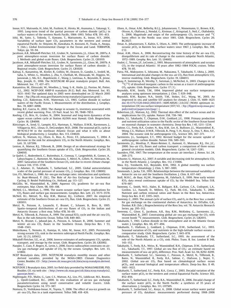
ARTICLE IN PRESS

T. Takahashi et al. / Deep-Sea Research II 56 (2009) 554–577576

Inoue, H.Y., Matsueda, H., Ishii, M., Fushimi, K., Hirota, M., Asanuma, I., Takasugi, Y.,1995. Long-term trend of the partial pressure of carbon dioxide (pCO2) insurface waters of the western North Pacific, 1984–1993. Tellus 47B, 391–413.

Ishii, M., Saito, S., Tokieda, T., Kawano, T., Matsumoto, K., Inoue, H.Y., 2004.Variability of surface layer CO2 parameters in the western and centralequatorial Pacific. In: Shiyomi, M., Kawahata, H., Koizumi, H., Tsuda, A., Awaya,Y. (Eds.), Global Environmental Change in the Ocean and Land. TERRAPUB,Tokyo, pp. 59–94.

Jacobson, A.R., Mikaloff-Fletcher, S.E., Gruber, N., Sarmiento, J.L., Gloor, M., 2007a. Ajoint atmosphere–ocean inversion for surface fluxes of carbon dioxide:1. Methods and global-scale fluxes. Glob. Biogeochem. Cycles 21, GB1019.

Jacobson, A.R., Mikaloff-Fletcher, S.E., Gruber, N., Sarmiento, J.L., Gloor, M., 2007b. Ajoint atmosphere-ocean inversion for surface fluxes of carbon dioxide: 2.Regional results. Glob. Biogeochem. Cycles 21, GB1020.

Kalnay, E., Kanamitsu, M., Kistler, R., Collins, W., Deaven, D., Gandin, L., Iredell, M.,Saha, S., White, G., Woollen, J., Zhu, Y., Chelliah, M., Ebisuzaki, W., Higgins, W.,Janowiak, J., Mo, K.C., Ropelewski, C., Wang, J., Leetmaa, A., Reynolds, R., Jenne,Roy., Joseph, D., 1996. The NCEP/NCAR 40-year reanalysis project. Bull. Am.Meteorol. Soc. 77, 437–471.

Kanamitsu, M., Ebisuzaki, W., Woollen, J., Yang, S.-K., Hnilo, J.J., Fiorino, M., Potter,G.L., 2002. NCEP-DOE AMIP-II reanalysis (R-2). Bull. Am. Meteorol. Soc. 83,1631–1643 The updated data to 2005 were downloaded on 22 March 2005from /ftp://ftp.cdc.noaa.gov/Datasets/ncep.reanalysis2/gaussian.grid/S.

Keeling, C.D., Rakestraw, N.W., Waterman, L.S., 1965. Carbon dioxide in surfacewaters of the Pacific Ocean, 1. Measurements of the distribution. J. Geophys.Res. 70, 6087–6098.

Keeling, R.F., Garcia, H., 2002. The change in oceanic O2 inventory associated withrecent global warming. Proc. US Natl. Acad. Sci. 99, 7848–7853.

Keeling, C.D., Brix, H., Gruber, N., 2004. Seasonal and long-term dynamics of theupper ocean carbon cycle at Station ALOHA near Hawaii. Glob. Biogeochem.Cycles 18, GB4006.

Kortzinger, A., Send, U., Lampitt, R.S., Hartman, S., Wallace, D.W.R., Karstensen, J.,Villagarcia, M.G., Llinas, O., DeGrandpre, M.D., 2008. The seasonal pCO2 cycle at491N/16.51W in the northeast Atlantic Ocean and what it tells us aboutbiological productivity. J. Geophys. Res. 113, C04020.

Lefevre, N., Watson, A.J., Olsen, A., Rios, A., Perez, F.F., Johannessen, T., 2004. Adecrease in the sink for atmospheric CO2 in the North Atlantic. Geophys. Res.Lett. 31, L07306.

Lenton, A., Matear, R.J., Tilbrook, B., 2006. Design of an observational strategy forquantifying the Southern Ocean uptake of CO2. Glob. Biogeocehm. Cycles 20,GB4010.

Le Quere, C., Rodembeck, C., Buitenhuis, E., Conway, T., Langenfelds, R., Gomez, A.,Labuschagne, C., Ramonet, M., Nakazawa, T., Metzl, N., Gillett, N., Heimann, M.,2007. Saturation of the Southern Ocean CO2 sink due to recent climate change.Science 316, 1735–1738.

Li, Z., Adamec, D., Takahashi, T., Sutherland, S.C., 2005. Global autocorrelationscales of the partial pressure of oceanic CO2. J. Geophys. Res. 110, C08002.

Liss, P.S., Merlivat, L., 1986. Air–sea gas exchange rates: introduction and synthesis.In: Buat-Menard, P. (Ed.), The Role of Air–Sea Exchange in GeochemicalCycling. D. Reidel Publishing Co., Holland, pp. 113–127.

McGillis, W., Wanninkhof, R., 2006. Aqueous CO2 gradients for air–sea fluxestimates. Mar. Chem. 98, 100–108.

McNeil, C.L., Merlivat, L., 1996. The warm oceanic surface layer: implications forCO2 fluxes and surface gas measurements. Geophys. Res. Lett. 23, 3575–3578.

McNeil, B.I., Metzel, N., Key, R.M., Matear, R.J., Corbiere, 2007. An empiricalestimate of the Southern Ocean air–sea CO2 flux. Glob. Biogeochem. Cycles 21,GB3011.

Metzl, N., Poisson, A., Louanchi, F., Brunet, C., Schauer, B., Bres, B., 1995.Spatio–temporal distributions of air–sea fluxes of CO2 in the Indian andAntarctic Oceans: a first step. Tellus 47B, 56–69.

Metzl, N., Tilbrook, B., Poisson, A., 1999. The annual fCO2 cycle and the air–sea CO2

flux in the sub-Antarctic Ocean. Tellus 51B, 849–861.Metzl, N., Brunet, C., Jabaud-Jan, A., Poisson, A., Schauer, B., 2006. Summer and

winter air–sea CO2 fluxes in the Southern Ocean. Deep-Sea Res. I 53,1548–1563.

Midorikawa, T., Nemoto, K., Kamiya, H., Ishii, M., Inoue, H.Y., 2005. Persistentlystrong oceanic CO2 sink in the western subtropical North Pacific. Geophys. Res.Lett. 32 (5), L05612.

Mikaloff-Fletcher, S.E., et al., 2006. Inverse estimates of anthropogenic CO2 uptake,transport, and storage by the ocean. Glob. Biogeochem. Cycles 20, GB2002.

Naegler, T., Ciais, P., Rogers, K., Levin, I., 2006. Excess radiocarbon constrains on air-sea gas exchange and uptake of CO2 by the oceans. Geophys. Res. Lett. 33,LI1802.

NCEP Reanalysis data, 2001. NCEP/NCAR reanalysis monthly means and otherderived variables, provided by the NOAA-CIRES Climate DiagnosticsCenter, Boulder, CO /http://www.cdc.noaa.gov/cdc/data/ncep.reanalysis.derived.htmlS.

NCEP/DOE 2 Reanalysis data, 2005. Ice field data provided by NOAA/OAR/ESRL PSD,Boulder, CO, via web site: /http://www.cdc.noaa.gov/cdc/data.ncep.reanalysis2.gaussian.htmlS.

Nightingale, P.D., Malin, G., Law, C.S., Watson, A.J., Liss, P.S., Liddicoat, M.I., Boutin,J., Upsill-Goddard, R.C., 2000. In situ evaluation of air-sea gas exchangeparameterizations using novel conservative and volatile tracers. Glob.Biogeochem Cycles 14, 373–387.

Nomura, D., Yoshikawa-Inoue, H., Toyota, T., 2006. The effect of sea-ice growth onair–sea CO2 flux in a tank experiment. Tellus 58B, 418–426.

Olsen, A., Omar, A.M., Bellerby, R.G.J., Johannessen, T., Ninnemann, U., Brown, K.R.,Olsson, A., Olafsson, J., Nondal, G., Kivimae, C., Kringstad, S., Neil, C., Olafsdottir,S., 2006. Magnitude and origin of the anthropogenic CO2 increase and 13CSuess effect in the Nordic seas since 1981. Glob. Biogeochem. Cycles 20,BG3027.

Omar, A., Johannessen, T., Kaltin, S., Olsen, A., 2003. The anthropogenic increase ofoceanic pCO2 in Barents Sea surface waters since 1967. J. Geophys. Res. 108,C12.

Omar, A.M., Olsen, A., 2006. Reconstructing the time history of the air–sea CO2

disequilibrium and its rate of change in the eastern subpolar North Atlantic,1972–1989. Geophy. Res. Lett. 33, L04602.

Oudot, C., Ternon, J.F., LeComte, J., 1995. Measurements of atmospheric and oceanicCO2 in the tropical Atlantic: 10 years after 1982–1984 FOCAL cruises. Tellus47B, 70–85.

Patra, P.K., Maksyutov, S., Ishizawa, M., Nakazawa, T., Takahashi, T., Ukita, J., 2005.Interannual and decadal changes in the sea–air CO2 flux from atmospheric CO2

inverse modeling. Glob. Biogeochem. Cycles 19, GB4013.Quay, P., Sommerup, R., Westby, T., Sutsman, J., McNichol, A., 2003. Changes in the

13C/12C of dissolved inorganic carbon in the ocean as a tracer of anthropogenicCO2 uptake. Glob. Biogeochem. Cycles 17 (1).

Reynolds, R.W., Smith, T.M., 1994. Improved global sea surface temperatureanalyses using optimum interpolation. J. Clim. 7, 929–948.

Reynolds, R.W., Rayner, N.A., Smith, T.M., Stokes, D.C., Wang, W., 2003. Animproved in situ and satellite SST analysis for climate. J. Clim. 15, 1609–1625doi:10.1175/1520-0442(2002)015/1609:AIISASS2.0.CO2 (NOAA optimum in-terpolation (OI) sea surface temperature (SST) V2, /ftp://ftpprd.ncep.noaa.gov/pub/cmd/sst/papers/oiv2pap/S).

Robertson, J.E., Watson, A.J., 1992. Thermal skin effect of the surface ocean and itsimplications for CO2 uptake. Nature 358, 738–740.

Rubin, S.I., Takahashi, T., Chipman, D.W., Goddard, J.G., 1998. Primary productionand nutrient utilization ratios in the Pacific sector of the Southern Ocean basedon seasonal changes in seawater chemistry. Deep-Sea Res. I 45, 1211–1234.

Sabine, C.L., Feely, R.A., Gruber, N., Key, R.M., Lee, K., Bullister, J.L., Wanninkhof, R.,Wong, C.S., Wallace, D.W.R., Tilbrook, B., Peng, T.-H., Kozyr, A., Ono, T., Rios, A.F.,2004. The oceanic sink for anthropogenic CO2. Science 305, 367–371.

Sarmiento, J.L., Sundquist, E.T., 1992. Revised budget for the oceanic uptake ofanthropogenic carbon dioxide. Nature 356, 589–593.

Sarmiento, J.L., Monfray, P., Maier-Reimer, E., Aumont, O., Murnane, R.J., Orr, J.C.,2000. Sea–air CO2 fluxes and carbon transport: a comparison of three oceangeneral circulation models. Glob. Biogeochem. Cycles 14, 1267–1281.

Saunders, P.M., 1967. The temperature at the ocean–air interface. J. Atmos. Sci. 24,269–273.

Schuster, U., Watson, A.J., 2007. A variable and decreasing sink for atmospheric CO2

in the North Atlantic. J. Geophys. Res. 112, C11006.Shea, D.J., Trenberth, K.E., Reynolds, R.W., 1992. A global monthly sea surface

temperature climatology. J. Clim. 5, 987–1001.Simmonds, I., Jacka, T.H., 1995. Relationships between the interannual variability of

Antarctic sea ice and the Southern Oscillation. J. Clim. 8, 637–647.Stoll, M.H.C., de Baar, H.J.W., Hoppema, M., Fahrbach, E., 1999. New early winter

fCO2 data reveal continuous uptake of CO2 by the Weddell Sea. Tellus 51B,679–687.

Sweeney, C., Smith, W.O., Hales, B., Bidigare, R.R., Carlson, C.A., Codispoti, L.A.,Gordon, L.I., Hansell, D., Millero, F.J., Park, Mi.-O.K., Takahashi, T., 2000.Nutrient and carbon removal ratios and fluxes in the Ross Sea, Antarctica.Deep-Sea Res. II 47, 3395–3421.

Sweeney, C., 2003. The annual cycle of surface CO2 and O2 in the Ross Sea: a modelfor gas exchange on the continental shelves of Antarctica. In: DiTullio, G.R.,Dunbar, R.B. (Eds.), Biogeochemistry of the Ross Sea, vol. 78. Antarctic ResearchSeries, pp. 295–312.

Sweeney, C., Gloor, E., Jacobson, A.R., Key, R.M., McKinley, G., Sarmiento, J.L.,Wanninkhof, R., 2007. Constraining global air–sea gas exchange for CO2 withrecent bomb 14C measurements. Glob. Biogeochem. Cycles 21, GB2015.

Takahashi, T., 1961. Carbon dioxide in the atmosphere and in the Atlantic Oceanwater. J. Geophys. Res. 66, 477–494.

Takahashi, T., Olafsson, J., Goddard, J., Chipman, D.W., Sutherland, S.C., 1993.Seasonal variation of CO2 and nutrients in the high-latitude surface oceans: acomparative study. Glob. Biogeochem. Cycles 7, 843–878.

Takahashi, T., Takahashi, T.T., Sutherland, S.C., 1995. An assessment of therole of the North Atlantic as a CO2 sink. Philos. Trans. R. Soc. London B 348,143–152.

Takahashi, T., Feely, R.A., Weiss, R., Wanninkhof, R.H., Chipman, D.W., Sutherland,S.C., Takahashi, T.T., 1997. Global air–sea flux of CO2: an estimate based onmeasurements of sea–air pCO2 difference. Proc. Natl. Acad. Sci. 94, 8292–8299.

Takahashi, T., Sutherland, S.C., Sweeney, C., Poisson, A., Metzl, N., Tillbrook, B.,Bates, N., Wanninkhof, R., Feely, R.A., Sabine, C., Olafsson, J., Nojiri, Y.,2002. Global sea–air CO2 flux based on climatological surface oceanpCO2, and seasonal biological and temperature effects. Deep-Sea Res. II 49,1601–1622.

Takahashi, T., Sutherland, S.C., Feely, R.A., Cosca, C., 2003. Decadal variation of thesurface water pCO2 in the western and central Equatorial Pacific. Science 302,852–856.

Takahashi, T., Sutherland, S.C., Feely, R.A., Wanninkhof, R., 2006. Decadal change ofthe surface water pCO2 in the North Pacific: a synthesis of 35 years ofobservations. J. Geophys. Res. 111, C07S05.

Takahashi, T., Sutherland, S.C., Kozyr, A., 2008. Global ocean surface water partialpressure of CO2 database: measurements performed during 1968–2006

ARTICLE IN PRESS

T. Takahashi et al. / Deep-Sea Research II 56 (2009) 554–577 577

(Version 1.0). ORNL/CDIAC-152, NDP-088. Carbon Dioxide Information AnalysisCenter, Oak Ridge National Laboratory, US Department of Energy, Oak Ridge, TN,20pp.

Thiele, G., Roether, W., Schlosser, P., Kuntz, R., Siedler, G., Stramma, L., 1986.Baroclinic flow and transient-tracer fields in the Canary-Cape Verde Basin.J. Phys. Ocean. 16, 814–826.

Toggweiler, J.R., Dixon, K., Bryan, K., 1989. Simulations of radiocarbon in a coarseresolution world ocean model I: steady state pre-bomb distributions.J. Geophys. Res. 94, 8217–8242.

Wanninkhof, R., 1992. Relationship between wind speed and gas exchange.J. Geophys. Res. 97, 7373–7382.

Wanninkhof, R., McGillis, W.M., 1999. A cubic relationship between gas transferand wind speed. Geophys. Res. Lett. 26, 1889–1892.

Wanninkhof, R.H., Sullivan, K.F., Top, Z., 2004. Air–sea gas transfer in the SouthernOcean. J. Geophys. Res. 109 (C8), C08S19.

Wanninkhof, R., 2007. The impact of different gas exchange formulations and windspeed products on global air–sea CO2 fluxes. In: Garbe, C.S., Handler, R.A.,Jahne, B. (Eds.), Transport at the Air Sea Interface: Measurements, Models andParameterizations. Springer, Heidelberg, p. 320.

Ward, B., Wanninkhof, R., McGillis, W.R., Jessup, A.T., DeGrandpre, M.D., Hare, J.E.,Edson, J.B., 2004. Biases in the air–sea flux of CO2 resulting from ocean surfacetemperature gradients. J. Geophys. Res. 109, C8S08.

Weiss, R.F., 1974. Carbon dioxide in water and seawater: the solubility of a non-ideal gas. Mar. Chem. 2, 203–215.

Weiss, R.F., Price, B.A., 1980. Nitrous oxide solubility in water and seawater. Mar.Chem. 8, 347–359.

Yuan, X., Martinson, D.G., 2000. Antarctic sea ice extent variability and its globalconnectivity. J. Clim. 13, 1697–1717.

Zhang, X., Cai, W.-J., 2007. On some biases of estimating the global distribution ofair–sea CO2 flux by bulk parameterization. Geophys. Res. Lett. 34, L01608.