PBL/Alterra Note Climate effects of wood used for bioenergy Jan P.M. Ros1 Jelle G. van Minnen1

Eric J.M.M. Arets2

1. PBL Netherlands Environmental

Assessment Agency 2. Alterra, Wageningen University and

Research Centre PBL Publication number: 1182 Alterra report: 2455 August 2013

Climate effects of wood used for bioenergy © PBL Netherlands Environmental Assessment Agency The Hague/Bilthoven, 2013 PBL publication number: 1182 Alterra report: 2455 Corresponding author Jan.ros@pbl.nl Authors Jan P.M. Ros Jelle G. van Minnen Eric J.M.M. Arets Supervisor Pieter A. Boot Acknowledgements For their useful comments we like to thank: Jan Oldenburger – Probos Joop Spijker – Alterra Jan Peter Lesschen – Alterra Kees Boon – AVIH Allesandro Agostini – JRC Guiliana Zanchi – Lund University Patrick Lamers – Utrecht University Martin Junginger – Utrecht University Helena Chum – IEA WG, NREL, United States Annette Cowie – IEA WG, University of New England, Australia Robert Matthews – UK Forest Service Gert-Jan Nabuurs – Alterra Graphics PBL Beeldredactie Production coordination PBL Publishers This publication can be downloaded from: www.pbl.nl/en. Parts of this publication may be reproduced, providing the source is stated, in the form: PBL/Alterra (2013), Climate effects of wood used for bioenergy, PBL publication number 1182, Alterra report 2455. The Hague: PBL Netherlands Environmental Assessment Agency. PBL Netherlands Environmental Assessment Agency is the national institute for strategic policy analyses in the fields of the environment, nature and spatial planning. We contribute to improving the quality of political and administrative decision-making, by conducting outlook studies, analyses and evaluations in which an integrated approach is considered paramount. Policy relevance is the prime concern in all our studies. We conduct solicited and unsolicited research that is both independent and always scientifically sound.

3

Summary Wood growth and natural decay both take time, and this is an important aspect of sustainability assessments of wood used for energy. Wood taken from forests is a carbon-neutral energy source in the long term, but there are many examples of potential sources of wood used for bioenergy for which net emission reductions are not achieved in 10 to 40 years –the time frame for most climate policy mitigation targets. This is caused by two factors. The first factor relates to the fact that the carbon cycles of wood have a long time span. After final felling, CO2 fixation rates are initially relatively low, but increase again as forests regrow. This regrowth takes many years, sometimes more than a century. Wood residues can either be used or left in the forest. By using them, the emissions from the otherwise decaying residues (taking 2 to 30 years) would be avoided. The second factor concerns the fact that, if the wood is used for bioenergy, then fossil-energy emissions are being avoided. However, the direct emission levels from bioenergy are higher than those related to the fossil energy it replaces. These additional emissions also have to be compensated. The carbon debt caused by both factors has to be paid back first, before actual emission reductions can be realised. For wood residues (from harvesting or thinning) that are used to replace coal or oil products, these payback times are relatively short, of the order of 5 to 25 years, mainly depending on location and type of residue (longer if they replace gas). This is also the case when using wood from salvage logging. In most cases, when using wood from final felling directly for energy production, payback times could be many decades to more than a century, with substantial increases in net CO2 emissions, in the meantime. This is especially the case for many forests in Europe, because they are currently an effective carbon sink. Additional felling reduces average growth rates in these forests and thus the sequestration of carbon. The same is likely to be true for managed forests in other temperate regions. If wood from additional felling is used, it would be most effective to use it in products that stay in circulation for a long time, only to be used for energy at the end of its service life. An increase in wood demand may lead to an intensification of forest management, which may temporarily increase carbon sequestration rates and biomass yields. This would eventually reduce the payback times. However, it must be noted that it would still take a substantial amount of time for the intensification of forest management to become effective, especially when it includes drastic measures, such as converting natural forests into plantations. Short rotation plantations with fast growing trees on agricultural land may be another option, but in these cases there are similarities with the direct and indirect land-use change effects related to energy crops. Further analysis is required to enable a clear judgment on the impact of these options. Products are not the only place of storing carbon with a beneficial effect on climate change. The combination of bioenergy and carbon capture and storage (CCS) on large industrial sites where biomass is converted into energy carriers, such as transport fuel and electricity, is projected to be beneficial, as well. Even landfill sites may serve as storage of carbon in wood waste, as pieces of wood hardly degrade.

4

1 Introduction As the transition towards a low-carbon economy moves forward and the share of renewable energy sources within the system is increasing, the future availability of sustainable biomass is receiving more attention. Biomass is generally considered as a ‘carbon neutral’ energy source, because the carbon that is emitted during biomass incineration was only sequestered shortly before, or will be resequestered shortly afterwards. Recent studies, however, have questioned this carbon neutrality and show that this is only true to a certain extent. This is related to two issues that potentially complicate the use of bioenergy. One of which is that of direct and indirect land-use change caused by biomass cultivation, mainly for crops but presumably also for fast growing wood plantations – when established on formerly agricultural land. The other issue relates to the temporal imbalance in the carbon cycle, mainly for wood. Both aspects are crucial in the mitigation of climate change and global warming and should therefore be considered in sustainability criteria for bioenergy. The Dutch Ministry of Infrastructure and the Environment has requested PBL to present an overview of the impact of wood used for bioenergy on greenhouse gas emissions and climate change. At the same time, NL Agency assigned Alterra Wageningen UR to support PBL in this process. The main objective of this publication is to provide the parties involved with information that is relevant in the process of setting sustainability criteria for using wood as a biomass source for energy. This PBL–Alterra Note focuses on the potential effects on CO2 emissions and climate change of using wood from different sources. Current wood use and its actual effects were not evaluated. Other ecological, social or economic impacts that also could be relevant for sustainable development are not discussed here. A short overview of the most important aspects of carbon balances for wood and the resulting CO2 flows is presented, as well as a number of other relevant issues for climate change and their policy implications. The overview is based on the literature, including recent reviews of scientific information, in combination with additional model calculations and analyses. Addressing all details and variations that may occur in practice or presenting a complete review of the consequences of all possible and very specific forest management options was not possible within the scope of this study.

5

2 Problem definition and readers guide In the current framework of European energy policy, biogenic CO2 emissions from the combustion of biomass – wooded biomass included – are set to zero. This assumption of 'carbon neutrality' originates from the national greenhouse gas inventories of the United Nations Framework Convention on Climate Change (UNFCCC). In the case of the dedicated harvesting of wood for bioenergy purposes, this carbon neutrality has been questioned (e.g. Zanchi et al., 2011). In this respect, the term 'carbon debt' has been introduced, which has somewhat negative connotations, but also implies it can be 'paid off', over time (the payback time). Sometimes it is referred to as a 'carbon investment'. Box 1. What is a carbon debt? The carbon debt related to wood depends on two factors: 1) When timber is harvested, the biomass decreases. The amount of regrowth that would be needed to

recover from this decrease takes time. In addition, the growth rates of more mature forests are higher than those of regrowing forests, which temporarily reduces carbon sequestration capacity (see Chapter 3).

2) The CO2 emissions from bioenergy per unit of energy produced are generally higher than those from the replaced fossil fuels (see chapter 4).

This implies that compensating for the additional emissions from bioenergy takes time. In the meantime, the CO2 emitted from burning the harvested wood will remain in the atmosphere, thus contributing to the greenhouse effect The payback time is a way of quantifying this temporal effect, as described in Chapter 4. Often, only the first point is regarded as the carbon debt, but the term is also used in relation to the second point. See Annex A for more information on definitions. This carbon debt or investment is dependent on many factors, such as forest characteristics, tree species, type of forest management and method and timing of harvesting, i.e. whether the wood biomass originates from intermediary thinning, from the final felling of roundwood, or from the use of harvest residues. Carbon balances in forests can be analysed on stand level or landscape level (see Box 1). Additional energy sources are other woody residues, such as sawdust (pellets) from sawmills, and industrial or even household waste. In addition to information reviewed from scientific publications, we included new results based on a modelling experiment (using the EFISCEN model; see Annex C for details on model calculations) to assess potential impacts of increasing wood harvests in a range of contrasting European forest types. The scenarios used include additional harvesting for bioenergy from final felling, thinning and harvest residues (including dead wood). Under a strongly increasing demand for wood to be used for bioenergy and related effects on wood prices, it is not unimaginable that all of these types of wood will be considered as an energy resource, even if not used as such today. Furthermore, we calculated time-dependent emissions and emission reductions with a simple model simulating the use of forest residues and woody waste.

6

Box 2. Landscape level and stand level When assessing carbon balances in forests, a distinction is often made between stand level and landscape level. Stand levels are especially useful for analysing well-defined specific (model) situations and for studying time-dependent processes. Here, the focus is on a single tree or a small well-defined area of (even-aged) trees. Landscape levels are larger in scale and concern a complete forest or even a whole region. These landscapes may include many different stands with different properties, i.e. different species, age classes and management regimes. On stand level, the harvested trees will show a net decrease in carbon stocks for which the carbon debt can be calculated. On landscape level, a net accumulation of carbon in biomass can be realised if the volume of wood that is harvested annually is less than or equal to the annual increment in wood volume. Under such circumstances and on a landscape scale, forests usually act as net carbon sinks. Increased harvesting on a landscape level may still result in increasing carbon stocks, as long as the harvested volumes are lower than the net annual increment. Such increases, however, will result in changes in the equilibrium between harvest and increment and in a decrease in carbon stocks compared to the situation without additional harvesting. Here, we consider the forest on a landscape level as the more appropriate scale to assess effects of using wood as an energy source on greenhouse gas emissions. The EFISCEN model simulates developments in carbon stocks for living biomass pools (i.e. the growing forest), dead biomass (i.e. litter and standing dead trees), soil and wood harvests on landscape level, and allows comparisons between different harvesting scenarios. For analyses and calculations, on landscape level, of the impact of additional wood harvesting, it is important to clearly define the reference situation as well as the criteria. Here, this is illustrated for relatively young European forests (see Annex C for a description of the reference situation and scenarios applied). Section 3 first introduces the effects of using wood from final felling, intermediate thinning, harvest residues and woody wastes on the carbon balances. This subsequently provides information on the potential impact of CO2 emissions under an increasing demand for wood. In addition, the main characteristics of wood production and consumption, from forest to waste treatment, are introduced. Section 4 describes the different options for using this biomass as an energy source, thus substituting fossil fuels, and gives the corresponding fossil carbon displacement factors (expressing the differences in efficiency). In combination with the carbon balance data in Section 3, this information is used to quantify net greenhouse gas balances. Section 5 discusses the main implications for climate policy as well as the sustainability criteria. Section 6 addresses the main conclusions. Different metrics are possible to quantify the effects (see Annex 1). Chapter 3 discusses the ratio between carbon losses from the forest system and harvested carbon. Section 4 describes the issue of 'payback time', which is the time that would be needed to pay off a 'carbon debt'.

7

3 Impact of harvesting woody biomass

3.1 Introduction This chapter assesses the impacts of increased wood harvesting on carbon balances. It is important to note that the starting point for calculations and accounting is the present situation, because current decisions on the use of energy sources will have an effect on future emission reductions and will not affect the amount of carbon that has already been sequestered in tree biomass in the past.

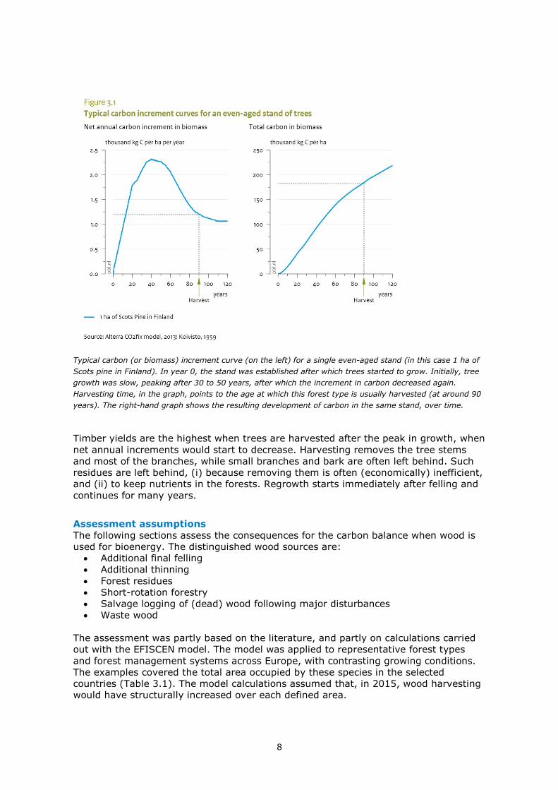
3.2 Forest growth and carbon sequestration Forests store large quantities of carbon, which was one of the reasons to include their state and management in the Kyoto Protocol (UNFCCC, 1997). Forests can act either as a carbon source or sink, depending on the balance between uptake of carbon through photosynthesis and the release of carbon through respiration, decomposition, fires, or removal through harvesting activities. In general, forests are estimated to have acted as sinks over the last decades, on both a European and global scale (Nabuurs et al., 2003; IPCC, 2007; Le Quéré et al., 2013). Different types of forest management can influence its carbon balance (Thornley and Cannell, 2000; Eggers et al., 2007). This is acknowledged in Articles 3.3 and 3.4 of the Kyoto Protocol. Forest management activities can influence carbon pools, fluxes and productivity, either directly, for example, by transferring carbon from 'growing stock' to '‘product' pools (e.g. through thinning or final harvesting), or indirectly, by altering tree growth conditions (e.g. through liming or fertilising). Effects can be immediate (e.g. from thinning) or evolve slowly (e.g. due to fertilisation). Activities may affect current stands (e.g. thinning regime) or future stands (e.g. regeneration), or may be transient (e.g. minimising site preparation, planting). Furthermore, impacts may be observed on stand level, but may also show additional feedback mechanisms on landscape level. Tree growth is one of the main processes that determine a forest's net carbon sequestration potential. This growth is not constant over time (Figure 3.1; the shape of the curve is characteristic for all types of tree species). Small trees in young forest stands sequester relatively little carbon. The rate of net biomass increment in these young forests increases up to a maximum, which is species and site specific. After the peak in growth at intermediary ages, growth rates gradually decrease again. In very old forests, net increment (balance between losses, disturbances and tree mortality, and the growth of individual trees) will further decrease and could become zero. This situation occurs only seldom in European forests, as they are usually harvested in rotations of a certain time span, the length of which depends on species, growth rate and the tree size required for the intended purpose (see also Table 3.1 for some characteristic values of rotation periods).

8

Typical carbon (or biomass) increment curve (on the left) for a single even-aged stand (in this case 1 ha of Scots pine in Finland). In year 0, the stand was established after which trees started to grow. Initially, tree growth was slow, peaking after 30 to 50 years, after which the increment in carbon decreased again. Harvesting time, in the graph, points to the age at which this forest type is usually harvested (at around 90 years). The right-hand graph shows the resulting development of carbon in the same stand, over time. Timber yields are the highest when trees are harvested after the peak in growth, when net annual increments would start to decrease. Harvesting removes the tree stems and most of the branches, while small branches and bark are often left behind. Such residues are left behind, (i) because removing them is often (economically) inefficient, and (ii) to keep nutrients in the forests. Regrowth starts immediately after felling and continues for many years.

Assessment assumptions The following sections assess the consequences for the carbon balance when wood is used for bioenergy. The distinguished wood sources are:

• Additional final felling • Additional thinning • Forest residues • Short-rotation forestry • Salvage logging of (dead) wood following major disturbances • Waste wood

The assessment was partly based on the literature, and partly on calculations carried out with the EFISCEN model. The model was applied to representative forest types and forest management systems across Europe, with contrasting growing conditions. The examples covered the total area occupied by these species in the selected countries (Table 3.1). The model calculations assumed that, in 2015, wood harvesting would have structurally increased over each defined area.

9

Table 3.1

Species selected for the modelling of the effects of different harvesting scenarios on

carbon dynamics

Species Region/

country Total area covered

(1000 ha)

Growth Rotation (in years)

Sitka spruce Scotland 800 Fast 40–60

Beech Germany 1560 Relatively slow 120–140

Norway spruce Germany 2980 Relatively fast 80–120

Scots pine Finland 10560 Slow 76–90

Scots pine Poland 4320 Moderate 80–120

Oak coppice Bulgaria 540 Slow 60–90

Maritime pine France 1360 Fast 45–55

Poplar France 140 Fast 20–25

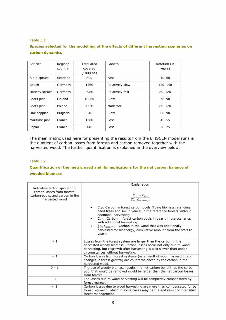
The main metric used here for presenting the results from the EFISCEN model runs is the quotient of carbon losses from forests and carbon removed together with the harvested wood. The further quantification is explained in the overview below. Table 3.2

Quantification of the metric used and its implications for the net carbon balance of

wooded biomass

Indicative factor: quotient of carbon losses from forests,

carbon pools, and carbon in the harvested wood

Explanation

𝐶𝑟(𝑡) − 𝐶𝑠(𝑡)

∑ 𝐶ℎ𝑎𝑟𝑣𝑒𝑠𝑡(𝑡)𝑛𝑡=1

• Cr(t): Carbon in forest carbon pools (living biomass, standing

dead trees and soil in year t, in the reference forests without additional harvesting

• Cs(t): Carbon in forest carbon pools in year t in the scenarios with additional harvesting.

• ∑ 𝐶ℎ𝑎𝑟𝑣𝑒𝑠𝑡(𝑡)𝑛𝑡=1 : Carbon in the wood that was additionally

harvested for bioenergy, cumulative amount from the start to year t.

> 1 Losses from the forest system are larger than the carbon in the

harvested woody biomass. Carbon losses occur not only due to wood harvesting, but regrowth after harvesting is also slower than under circumstances without harvesting.

= 1 Carbon losses from forest systems (as a result of wood harvesting and changes in forest growth) are counterbalanced by the carbon in the harvested wood.

0 – 1 The use of woody biomass results in a net carbon benefit, as the carbon pool that would be removed would be larger than the net carbon losses from forests

0 The losses due to wood harvesting will be completely compensated by forest regrowth

< 1 Carbon losses due to wood harvesting are more than compensated for by forest regrowth, which in some cases may be the end result of intensified forest management

10

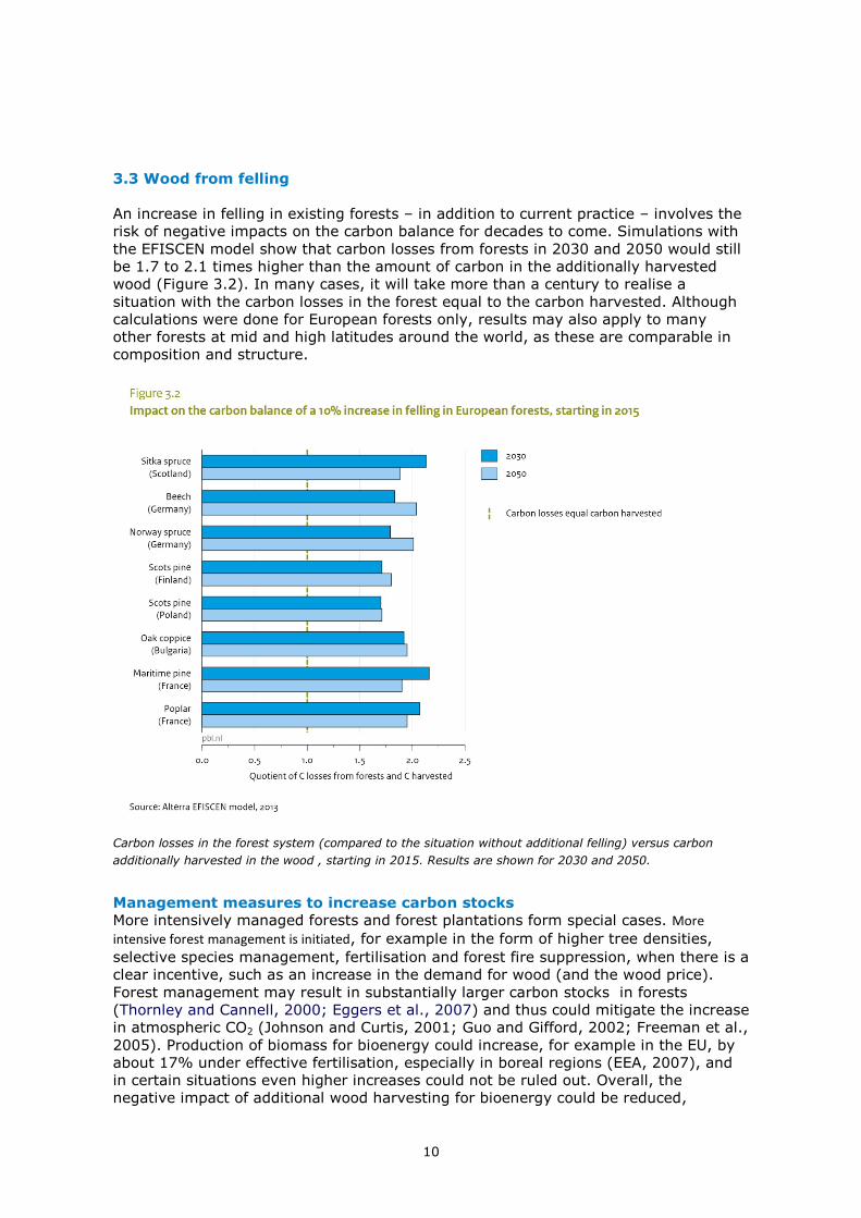
3.3 Wood from felling An increase in felling in existing forests – in addition to current practice – involves the risk of negative impacts on the carbon balance for decades to come. Simulations with the EFISCEN model show that carbon losses from forests in 2030 and 2050 would still be 1.7 to 2.1 times higher than the amount of carbon in the additionally harvested wood (Figure 3.2). In many cases, it will take more than a century to realise a situation with the carbon losses in the forest equal to the carbon harvested. Although calculations were done for European forests only, results may also apply to many other forests at mid and high latitudes around the world, as these are comparable in composition and structure.

Carbon losses in the forest system (compared to the situation without additional felling) versus carbon additionally harvested in the wood , starting in 2015. Results are shown for 2030 and 2050.

Management measures to increase carbon stocks More intensively managed forests and forest plantations form special cases. More intensive forest management is initiated, for example in the form of higher tree densities, selective species management, fertilisation and forest fire suppression, when there is a clear incentive, such as an increase in the demand for wood (and the wood price). Forest management may result in substantially larger carbon stocks in forests (Thornley and Cannell, 2000; Eggers et al., 2007) and thus could mitigate the increase in atmospheric CO2 (Johnson and Curtis, 2001; Guo and Gifford, 2002; Freeman et al., 2005). Production of biomass for bioenergy could increase, for example in the EU, by about 17% under effective fertilisation, especially in boreal regions (EEA, 2007), and in certain situations even higher increases could not be ruled out. Overall, the negative impact of additional wood harvesting for bioenergy could be reduced,

11

considerably, under additional management (Tromberg et al., 2011; Jonker, 2013; JRC, 2013). In the long term, more intensive management in some cases may even lead to both a larger wood harvest and an increase in carbon stocks. Such a development may be driven by an increase in the demand for wood. However, converting natural forests into forest plantations takes time, as well, and does not exclude certain periods in which carbon losses from those forests will be higher than the amounts of carbon removed in wood that is harvested Within the context of the limited timeframe of this study, this could not be quantified more accurately. Furthermore, the conversion of natural forests into forest plantations also has other impacts than those from changes in carbon stocks (i.e. on biodiversity). Those other impacts could also be included in sustainability criteria.

Albedo effect One other aspect of additional final felling has to be mentioned in relation to climate change, specifically in boreal areas; namely that of the albedo effect (i.e. the reflection of sunlight, especially in the case of snow). This effect has an important impact on global warming. Because of final felling, the area of snow-covered land – the reflective area – is temporarily increased. Cherubini et al. (2012) report a relevant positive impact on global warming; in some cases, of the same order of magnitude as the greenhouse effect potentially caused by the CO2 emissions from burning the harvested wood.

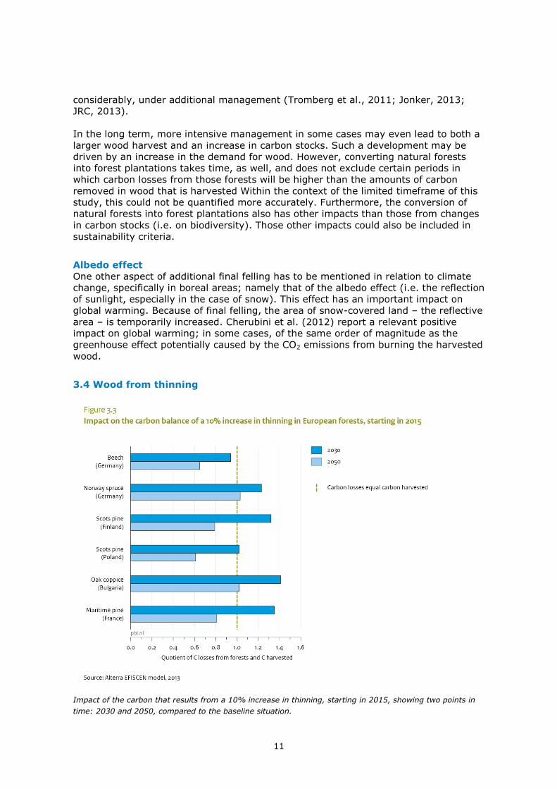
3.4 Wood from thinning

Impact of the carbon that results from a 10% increase in thinning, starting in 2015, showing two points in time: 2030 and 2050, compared to the baseline situation.

12

3.5 Logging and harvest residues Current global wood pellet production is predominantly residue-based (Lamers and Junginger, 2013). Harvest residues consist of remnants and portions of trees, such as tree tops, stumps, branches, foliage and pieces of bark, resulting from silvicultural activities (thinning and final felling). Currently, between 20% and 35% of total felling consists of residues (EUwood, 2010). Up to now, these residues often are left in the forest or burned along roadsides, because of their relatively low economic value. As such, forest residue potentially represents a substantial biomass resource that could be used to replace fossil fuel (Repo, 2012), even though only a part of it is easily accessible and could be harvested, from an ecological and economic perspective (Lippke et al., 2011). On balance, return periods will be short, as most of the carbon in tree harvest residues will be lost to the atmosphere, over a relatively short period of time, as a result of decomposition. The rate of decomposition differs, depending on factors such as climate, shape, size and type of residue (e.g. tree tops, branches, bark, roots, see Table 3.3) (Repo et al., 2012). In some cases, a small percentage of the carbon is released as CH4 (Spath and Mann (2001) report 10% from mulched wood). Table 3.3

Typical half-time values (in years) for the decay of wood residue in forests

Type of residue Half-time value (years)

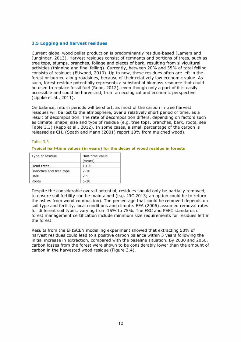
Dead trees 10-35 Branches and tree tops 2-10 Bark 2-5 Roots 5-20 Despite the considerable overall potential, residues should only be partially removed, to ensure soil fertility can be maintained (e.g. JRC 2013; an option could be to return the ashes from wood combustion). The percentage that could be removed depends on soil type and fertility, local conditions and climate. EEA (2006) assumed removal rates for different soil types, varying from 15% to 75%. The FSC and PEFC standards of forest management certification include minimum size requirements for residues left in the forest. Results from the EFISCEN modelling experiment showed that extracting 50% of harvest residues could lead to a positive carbon balance within 5 years following the initial increase in extraction, compared with the baseline situation. By 2030 and 2050, carbon losses from the forest were shown to be considerably lower than the amount of carbon in the harvested wood residue (Figure 3.4).

13

Impact of the carbon that results from a 50% removal of harvest residue, compared to a baseline situation without harvest residue removal; results are shown for two points in time: 2030 and 2050 As indicated above, in some cases, residues are not left in the forest but burned on site. In those cases, valorisation of the energy in the residue as a replacement of fossil fuel could lead to an emission reduction, but only if the extraction, pre-treatment and transport require less energy than the residue could provide.

3.6 Dead wood / salvage logging A special method of harvesting wood residues from forests is salvage logging, in which wood is removed that is damaged, dying or dead, due to for example storms, forest pathogens, insects and diseases. Dead wood includes wood lying on the forest floor (which otherwise would not be extracted), roots, and large stumps. Dead wood that remains in the forest has clear biodiversity benefits, but large amounts of dead wood may increase the risk of forest fires. In some cases, salvaged dead wood and decaying trees can still be used (e.g. after storms). According to the Food and Agriculture Organization (FAO) of the United Nations, the current global amount of dead wood is estimated at 67 Gt (although this figure is only a rough estimate), which is about 11% of the total in wooded biomass (FAO, 2010). Regions with large amounts of dead wood are located in Russia and parts of Africa. On a global level, close to 40 million hectares of forest are adversely affected by insect infestations and diseases, annually, but not all of these areas are equally accessible. The Mountain Pine Beetle in western North America is of special concern, because of the unprecedented magnitude of the infestations. Since the late 1990s, the beetle has devastated more than 11 million hectares of forest in Canada and the western United States, and it is still spreading today. In British Columbia, by 2012, the infestations had killed an estimated 710 million m3 of commercially valuable pine timber (IINAS,

14

2012; MFLNRO 2012; IEA, 2013). Some of this dead wood could be used in energy production (Lamers et al., 2013), resulting in a positive climate effect. Removing the dead trees would enable regrowth and/or replanting, thus increasing the average growth rate of the forest. Without salvage logging and clearing, decomposition in these forests, over time, could be a source of CO2 that is comparable to other residues. If this wood would otherwise be burned at the roadsides or be left in the forest without valorisation of its energy content, then any bioenergy alternative would be beneficial to the climate (Lamers et al. (2013) showed this for beetle-impacted pine forests in British Columbia). An important limitation to the use of salvaged wood from beetle-infested mountain pine forests will be the high costs associated with future harvests, as accessibility decreases and transport strongly increases (Niquidet et al., 2012).

3.7 New natural forests or forest plantations When new forests are planted, the CO2 uptake or carbon credit starts immediately (Mitchell et al., 2012; JRC, 2013). However, this also requires land, and the impact of direct or indirect land-use change has to be included in calculations of the carbon balance, similar to that related to biofuel production based on agricultural crops. Although, for the latter, CO2 emissions from indirect land-use change may be somewhat lower, as the carbon stock in forests is generally greater than in agricultural crops (IPCC, 2003). Indirect deforestation elsewhere also cannot be excluded. No (model) analysis is currently available that quantifies the overall and especially the indirect effect for new forests. It will take a while before new forests are able to provide wood as a resource for bioenergy. This period largely depends on the type of tree species and its rotation period. If, for example, relatively fast growing or short-rotation species (SRC) are selected, such as willow or eucalyptus, biomass becomes available relatively soon and on a regular basis (see also EEA, 2007). Multiple studies have shown that, on average, wood production in willow plantations is in the range of 6 to 15 t DM/ha yr (in energy terms, between 110 and 275 GJ/ha yr), harvested over 2 to 5-year cycles (e.g. Tsarev, 2005; Elbersen et al., 2013). The production range depends on location (production levels are lower in high-latitude countries) and, especially, on management intensity. High production levels are only possible if plantations are built on fertile (agricultural) land and with a high level of management (Dimitriou and Aronsson, 2005; Werner et al., 2012; Elbersen et al., 2013). Such short-rotation cultivation is like an agricultural activity and its level of sustainability should be judged in the same way, including the effects of indirect land-use change (ILUC), and considering the specific carbon stocks on such a plantation. As for other energy crops, willow plantations on marginal or degraded land (with production levels of around 6 to 9 t DM/ha yr) may be an interesting sustainable option to produce wooded biomass, but as business cases these are generally not very attractive, and it is difficult to formulate effective and enforceable criteria (PROBOS, 2009). It should be noted that, in boreal regions, the impact of the albedo effect in this case would be negative. The picture is different when existing, natural forests are converted into fast-growing plantations (Mitchell, et al., 2012), because all of the carbon stored in the original vegetation is lost. Wood production levels for bioenergy may be still high (although less than of plantations on agricultural land, as forested lands are often less fertile). However, the compensation of carbon losses due to the conversion would require a considerable period of time. For example, typical above-ground biomass pools in natural boreal and temperate forests contain, on average, about 60 and 150 t DM/ha, respectively (IPCC, 2003; FORM, 2013), which would equal a period of more than 10

15

years to compensate for the related carbon losses. A situation where more carbon is stored than is lost will seldom be reached, in the short term (Zanchi et al., 2012; JRC, 2013). Furthermore, these conversions often have considerable negative effects on other ecosystem goods and services, such as biodiversity (Brockerhoff et al., 2008).

3.8 Wood products and woody waste

Carbon stored in wood products Wood can be used as a building material, for all kinds of products (e.g. furniture), as well as for paper and cardboard. The carbon contained in these products remains effectively stored during their lifetimes, which vary from 1 to 10 years for most paper products, and between 20 and more than 100 years for some building materials. Even if the wood is burned in the end, the delay of the emission of the carbon that was temporarily stored in these products and materials can be quite relevant. If the carbon is stored in products that last for about 10 years, the impact of the related emissions on global warming 100 years from now will be reduced by almost 10%. If stored for 40 years, the impact will be reduced by about 30% (Cherubini et al., 2012), compared to the impact of an immediate CO2 emission at the time of harvesting. In practice, the use of wood can be optimised by the 'cascading principle', whereby the same wood is used in several successive applications. This is not only the case in paper recycling; wooden materials also can be recycled. Finally, waste wood and other woody residues from industry and households can be used for energy or, possibly, in the chemical industry. Burning the woody materials is the easiest way to use them. However, producing green polymer (e.g. polyethylene) from monomers in the chemical industry, or liquid and gaseous biofuels in the transport sector, or 'green' gas in various applications, may be more advantageous, because of a likely lack of low-carbon alternatives, in the coming decades, in these sectors. For those types of applications, more advanced technologies need to be implemented. CO2 conversion efficiency is about 50% to 60%, whereas carbon capture and storage or reuse would be an option that eliminates most of the emissions from industrial processes. Although, theoretically, the cascading principle is an attractive one, an optimal application of this principle requires that the demand for bioenergy becomes attuned to the use of wood as a resource material. Furthermore, our current society also is a carbon sink. More wooden materials enter the societal system than leave it as waste. An increase in the share of waste wood in the energy system, therefore, requires patience.

Woody waste The emission reduction achieved by using waste wood for energy is determined by the emission levels of the various alternatives, such as using incineration, landfill or composting. In case of waste incineration used for generating energy, the replacement of fossil fuels already leads to emission reductions. Reduction are being realised in many European waste incineration plants, today, but a higher level of efficiency could be reached by developing more dedicated installations. In the landfill option, some parts of the wood (cellulose and hemicellulose) can be degraded under the anaerobic conditions found in landfills. In practice, landfills serve as an effective carbon stock, because even after long periods of time most of the woody materials would still be present. Overall, between 25% and 35% of the carbon in woody forest products in landfills (consisting of large amounts of paper) is emitted (Micales and Skog, 1997; Mann and Spath, 2001). For solid pieces of wood within the waste, only a few per cent of the carbon would be released, even after many decades. The gases emitted from a landfill contain CO2 as well as CH4. Their ratio is strongly determined by local circumstances, such as moisture content, temperature and

16

anaerobic conditions. In practice, in many cases, 50% to 60% of the carbon is released in the form of methane (Micales and Skog, 1997; Mann and Spath, 2001). In some cases, methane partly will be recovered, especially in the first 5 to 20 years. For the greenhouse gas balances, related to woody waste used for energy, the avoidance of these methane emissions would be very relevant and advantageous (see Chapter 4 and Annex B).

17

4 Emission reduction and climate benefits of wood used for energy

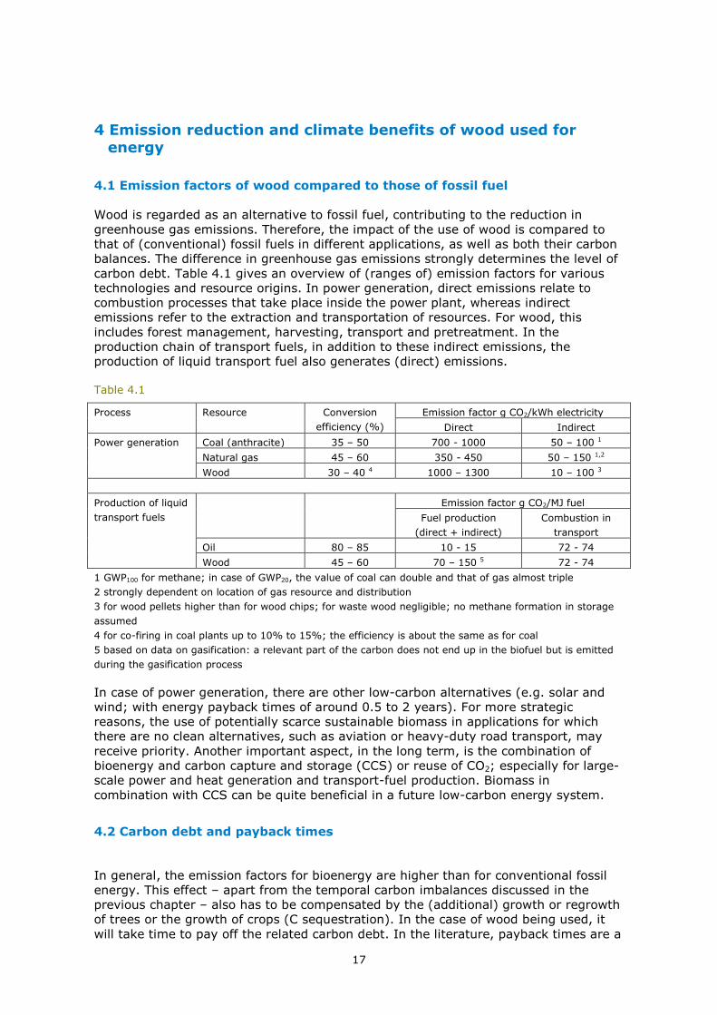
4.1 Emission factors of wood compared to those of fossil fuel Wood is regarded as an alternative to fossil fuel, contributing to the reduction in greenhouse gas emissions. Therefore, the impact of the use of wood is compared to that of (conventional) fossil fuels in different applications, as well as both their carbon balances. The difference in greenhouse gas emissions strongly determines the level of carbon debt. Table 4.1 gives an overview of (ranges of) emission factors for various technologies and resource origins. In power generation, direct emissions relate to combustion processes that take place inside the power plant, whereas indirect emissions refer to the extraction and transportation of resources. For wood, this includes forest management, harvesting, transport and pretreatment. In the production chain of transport fuels, in addition to these indirect emissions, the production of liquid transport fuel also generates (direct) emissions. Table 4.1

Process Resource Conversion efficiency (%)

Emission factor g CO2/kWh electricity Direct Indirect

Power generation Coal (anthracite) 35 – 50 700 - 1000 50 – 100 1 Natural gas 45 – 60 350 - 450 50 – 150 1,2 Wood 30 – 40 4 1000 – 1300 10 – 100 3

Production of liquid transport fuels

Emission factor g CO2/MJ fuel Fuel production

(direct + indirect) Combustion in

transport Oil 80 – 85 10 - 15 72 - 74 Wood 45 – 60 70 – 150 5 72 - 74

1 GWP100 for methane; in case of GWP20, the value of coal can double and that of gas almost triple 2 strongly dependent on location of gas resource and distribution 3 for wood pellets higher than for wood chips; for waste wood negligible; no methane formation in storage assumed 4 for co-firing in coal plants up to 10% to 15%; the efficiency is about the same as for coal 5 based on data on gasification: a relevant part of the carbon does not end up in the biofuel but is emitted during the gasification process In case of power generation, there are other low-carbon alternatives (e.g. solar and wind; with energy payback times of around 0.5 to 2 years). For more strategic reasons, the use of potentially scarce sustainable biomass in applications for which there are no clean alternatives, such as aviation or heavy-duty road transport, may receive priority. Another important aspect, in the long term, is the combination of bioenergy and carbon capture and storage (CCS) or reuse of CO2; especially for large-scale power and heat generation and transport-fuel production. Biomass in combination with CCS can be quite beneficial in a future low-carbon energy system.

4.2 Carbon debt and payback times

In general, the emission factors for bioenergy are higher than for conventional fossil energy. This effect – apart from the temporal carbon imbalances discussed in the previous chapter – also has to be compensated by the (additional) growth or regrowth of trees or the growth of crops (C sequestration). In the case of wood being used, it will take time to pay off the related carbon debt. In the literature, payback times are a

18

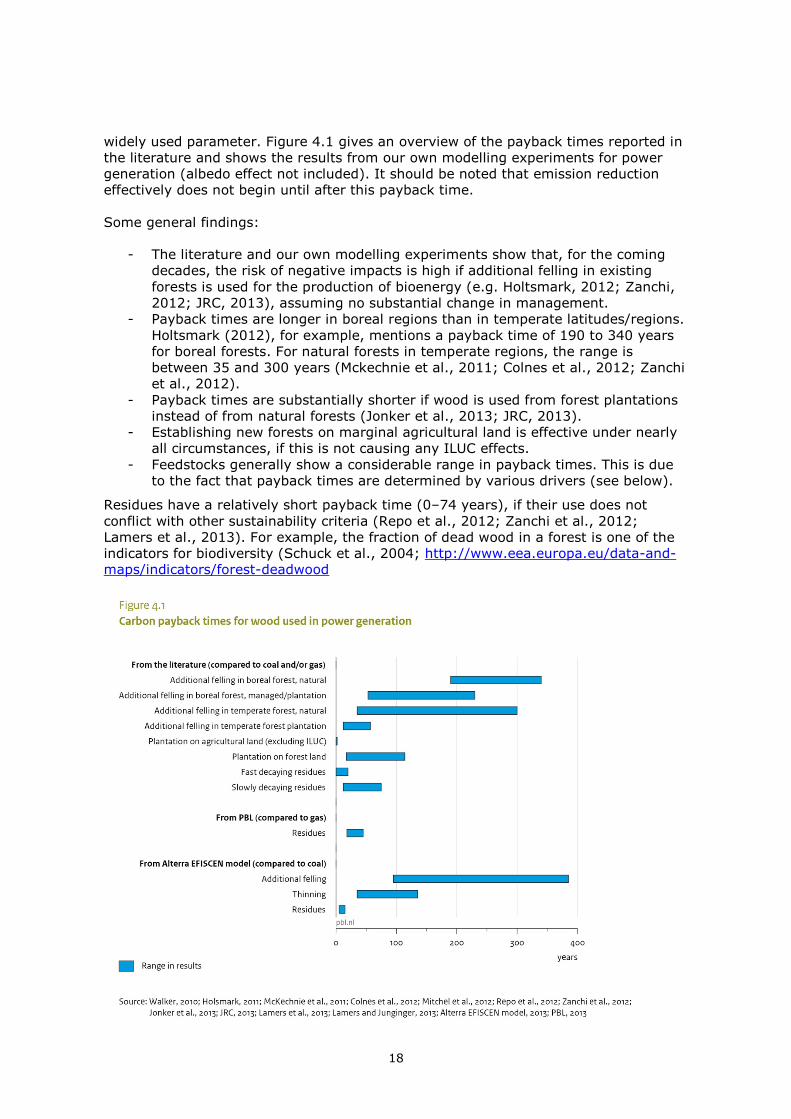
widely used parameter. Figure 4.1 gives an overview of the payback times reported in the literature and shows the results from our own modelling experiments for power generation (albedo effect not included). It should be noted that emission reduction effectively does not begin until after this payback time. Some general findings:

- The literature and our own modelling experiments show that, for the coming decades, the risk of negative impacts is high if additional felling in existing forests is used for the production of bioenergy (e.g. Holtsmark, 2012; Zanchi, 2012; JRC, 2013), assuming no substantial change in management.

- Payback times are longer in boreal regions than in temperate latitudes/regions. Holtsmark (2012), for example, mentions a payback time of 190 to 340 years for boreal forests. For natural forests in temperate regions, the range is between 35 and 300 years (Mckechnie et al., 2011; Colnes et al., 2012; Zanchi et al., 2012).

- Payback times are substantially shorter if wood is used from forest plantations instead of from natural forests (Jonker et al., 2013; JRC, 2013).

- Establishing new forests on marginal agricultural land is effective under nearly all circumstances, if this is not causing any ILUC effects.

- Feedstocks generally show a considerable range in payback times. This is due to the fact that payback times are determined by various drivers (see below).

Residues have a relatively short payback time (0–74 years), if their use does not conflict with other sustainability criteria (Repo et al., 2012; Zanchi et al., 2012; Lamers et al., 2013). For example, the fraction of dead wood in a forest is one of the indicators for biodiversity (Schuck et al., 2004; http://www.eea.europa.eu/data-and-maps/indicators/forest-deadwood

19

As mentioned above, the literature shows a considerable range in payback times. The reasons for this wide range are the following:

- The replacement of fossil fuel. Replacing coal by wooded biomass has a significantly shorter payback time than when replacing natural gas.

- Wood characteristics, such as moisture content. - The forest species and residue type considered. - Current and future forest growth rates. Using wood from relatively young, still

fast growing forests is less attractive. Given the fact that European forests are often in this phase, it would be more efficient, from the perspective of emission reduction, to leave the trees in the forest than to harvest them for energy.

- Management may increase forest growth rates and, thus, may shorten payback times, compared to those of unmanaged forests (see also Chapter 3; and JRC, 2013)

- For forest residues, particular and additional factors determine the payback time, due to differences in pool sizes, types of residues (fast decaying bark, twigs and leaves or slowly decaying dead stem wood or stumps), and alternative residue use (natural decay leads to longer payback times than when residues are burned on site without the energy being used).

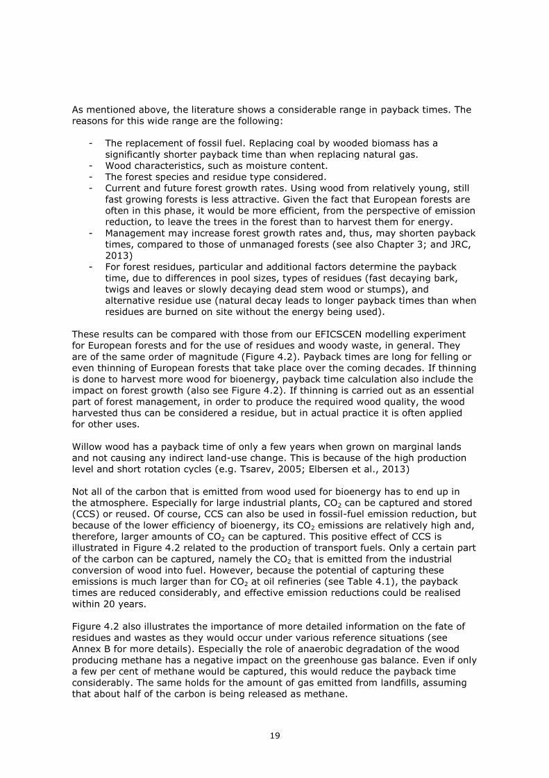
These results can be compared with those from our EFICSCEN modelling experiment for European forests and for the use of residues and woody waste, in general. They are of the same order of magnitude (Figure 4.2). Payback times are long for felling or even thinning of European forests that take place over the coming decades. If thinning is done to harvest more wood for bioenergy, payback time calculation also include the impact on forest growth (also see Figure 4.2). If thinning is carried out as an essential part of forest management, in order to produce the required wood quality, the wood harvested thus can be considered a residue, but in actual practice it is often applied for other uses. Willow wood has a payback time of only a few years when grown on marginal lands and not causing any indirect land-use change. This is because of the high production level and short rotation cycles (e.g. Tsarev, 2005; Elbersen et al., 2013) Not all of the carbon that is emitted from wood used for bioenergy has to end up in the atmosphere. Especially for large industrial plants, CO2 can be captured and stored (CCS) or reused. Of course, CCS can also be used in fossil-fuel emission reduction, but because of the lower efficiency of bioenergy, its CO2 emissions are relatively high and, therefore, larger amounts of CO2 can be captured. This positive effect of CCS is illustrated in Figure 4.2 related to the production of transport fuels. Only a certain part of the carbon can be captured, namely the CO2 that is emitted from the industrial conversion of wood into fuel. However, because the potential of capturing these emissions is much larger than for CO2 at oil refineries (see Table 4.1), the payback times are reduced considerably, and effective emission reductions could be realised within 20 years. Figure 4.2 also illustrates the importance of more detailed information on the fate of residues and wastes as they would occur under various reference situations (see Annex B for more details). Especially the role of anaerobic degradation of the wood producing methane has a negative impact on the greenhouse gas balance. Even if only a few per cent of methane would be captured, this would reduce the payback time considerably. The same holds for the amount of gas emitted from landfills, assuming that about half of the carbon is being released as methane.

20

Payback times calculated for wood waste (compared to storage in landfill) and residues used in the production of transport fuels (based on gasification)

4.3 Substituting wood for other materials Wood can also be used to replace materials such as steel or concrete, thereby avoiding the emissions from producing those materials. Sathre and O’Connor (2010) presented a survey on the impact of carbon emissions from various substitutions. They concluded that, in most cases, for every kilogram of carbon in wood, 1 to 3 kilograms (on average 2.1 kg) of carbon emissions from the production of alternative materials would be avoided. This would imply a short-term carbon credit. However, Figure 3.2 shows the relative carbon losses in European forests after 15 to 35 years also equal around twice the amounts of carbon in the harvested wood, implying a neutral situation for many substitutions over such time periods. This would be an investment in substantial emission reductions in the very long term.

21

5 Policy implications

Emissions related to bioenergy

The assumption that bioenergy would be climate neutral has been one of the reasons for emissions from the use of bioenergy being counted as zero, in turn leading to an increase in the demand for bioenergy. However, the assumption that all of the emitted CO2 from wood burning is reabsorbed by new and existing forests is only valid over very long periods of time – in some cases, over more than a century. For the short term, such an approach could present a wrong picture of the actual net emissions on an annual basis, because in many cases a carbon debt occurs, as also discussed in the previous chapters. However, there are also wooded biomass sources with much shorter payback times (see Chapters 3 and 4).

CO2 emissions from (wood-based) bioenergy are counted as being zero by the energy sector, in the emissions accounting methods of international climate conventions (both UNFCCC and Kyoto Protocol). This is agreed to prevent double counting the carbon emissions related to wood harvested for bioenergy; once under land-use change and again by the energy sectors. Under the United Nations' climate convention (UNFCCC), to which most countries report, these emissions are already counted at the time and place of wood harvesting. Developed countries that have ratified the Kyoto Protocol only report on the CO2 emissions and removals related to land that is subject to deforestation and/or reforestation/afforestation (cleared areas and subsequent regrowth included). In addition, countries can choose to report on forest management activities under Article 3.4 of the Kyoto Protocol if these activities result in changes in carbon stocks. During the first commitment period (2008-2012), forest management reporting was voluntary, whereas for the second commitment period this has become compulsory. Developing countries and developed countries that have not ratified (e.g. United States) or have withdrawn (e.g. Canada) from the protocol, do not have this obligation. As a consequence, there is a loophole in carbon emissions accounting when wood that is harvested in a country that has no obligation under the Kyoto Protocol is then shipped and burned in a country that has ratified the protocol. In those cases, carbon emissions from the use of bioenergy are not accounted for.

A change to the emissions accounting system could be considered. In general, there are two options for the emissions from wood:

1. Assessments could be added, containing data on actual emissions and sinks in non-Kyoto Protocol countries where wood is also being harvested and exported. This means that the wood trade would need to be monitored, and an independent authority would need to perform the necessary assessments.

2. Wood-based bioenergy emissions are only counted as zero if the wood originates from a country that has ratified the Kyoto Protocol; otherwise the actual emissions are counted. It would make the use of this biomass unattractive as a measure to reduce greenhouse gas emissions. This may stimulate exporting countries to join such international agreements.

Sustainability criteria for solid biomass

The certification schemes of sustainable forest management, such as PEFC and FSC, do not include net greenhouse gas emissions. However, there are criteria for forest management, such as whether wood residues are removed from the forest or not, and the setting of sustainable extraction rates of these residues. Large areas of European forests have been certified already. These criteria also can be used to avoid unacceptable forest quality

22

losses. This PBL/Alterra note does not include an evaluation of the impact of these guidelines on the potential of using wood residues in energy generation. Forest plantations of fast growing trees, such as willows, have many similarities with energy crop farming. The direct and indirect effects of land-use change could be included in sustainability criteria, in the same way (at the time of publication, no final decision had been made on ILUC in the sustainability criteria for biofuels), taking into account the specific characteristics of these plantations, especially related to carbon storage, and the impact on agricultural markets.

Greenhouse gas emissions in sustainability criteria for biofuels

The sustainability criteria for transport biofuels in EU policy include a minimum greenhouse gas emission reduction compared to those for fossil fuels. Until recently, the reduction percentage was 35%, but this has meanwhile increased to up to 60%. Also, in this case, the CO2 exhaust emissions from biofuel related to road traffic have been set to zero. Based on this assumption, biofuels (ethanol or biodiesel) produced from wood resources could meet this criterion. However, if time dependency would be included, this is not automatically the case. For land-use change emissions, the criteria refer to a period of 20 years. If the same period is applied for the time dependent emissions related to wood, the expected emission reductions, in many cases, would be much lower (see also Annex B).

However, emission reductions related to wood residues or wood waste are strongly dependent on assumptions with respect to the reference situation, the rate of decay in forests and landfills, and the formation of methane (see Annex B for more details). Emission reductions of 60% or more in relation to biofuels from wood sources would be difficult to guarantee, and would strongly depend on the reference situations. Furthermore, if there are no other clean fuel alternatives for some of the transport modes, from the perspective of climate change, any emission reduction would be an improvement. Therefore, using 60% emission reduction as a criterion for the sustainability of wood residues or wood waste for transport fuels should be reconsidered.

The application of carbon capture and storage (CCS) or reuse of CO2 in biofuel production (such as through a gasification process) is relatively effective, because a considerable fraction of the carbon does not end up in the produced fuel but is captured. The use of forest residues would lead to emission reductions of 50% to 100% in the first 20 years (even if CCS is also assumed for oil refineries in the reference situation).

Forest cultivation with short rotation times, such as that of willows, could provide biomass for transport fuels. Results from sustainability assessments of this type of cultivation should be similar to those of agricultural crops, especially for land-use related emissions. Currently, there are no model simulations available that quantify ILUC effects on a global scale. If willow plantations are started on existing agricultural land, these effects are likely to occur and the impact on the greenhouse gas balance would also be relevant.

23

6 Conclusions

Emissions accounting of wood-based bioenergy provides an inaccurate picture of the net carbon balance between land and atmosphere.

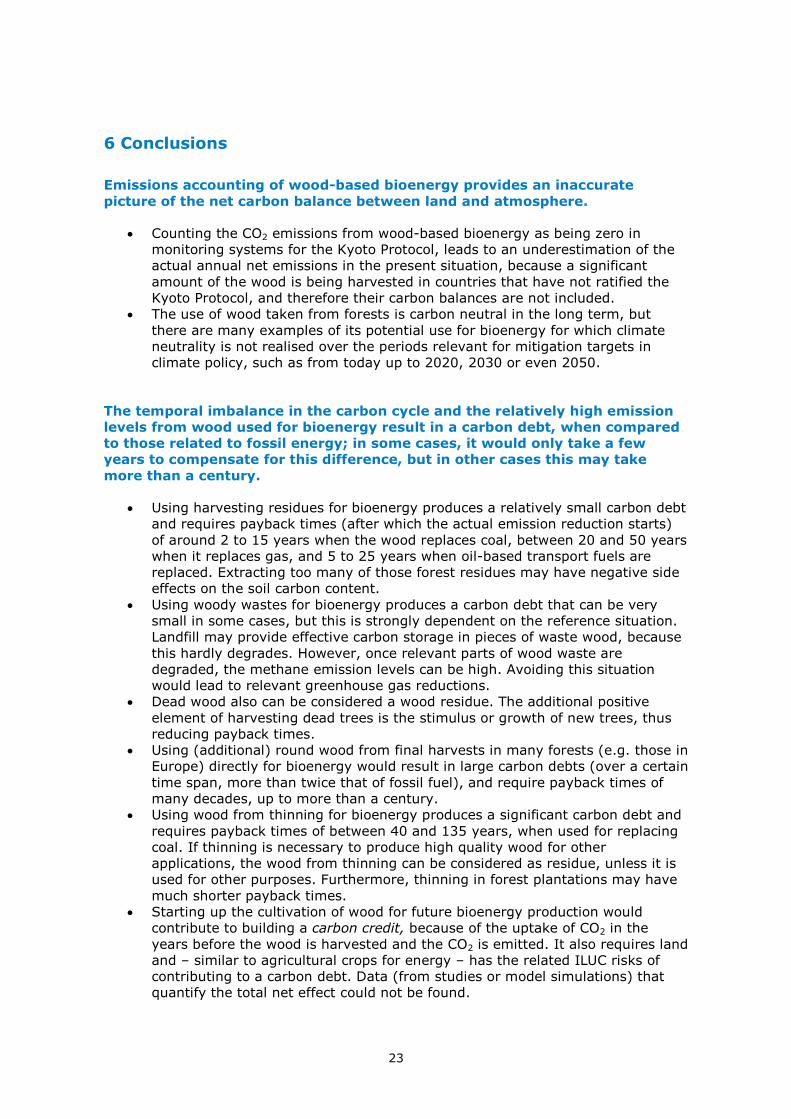
• Counting the CO2 emissions from wood-based bioenergy as being zero in monitoring systems for the Kyoto Protocol, leads to an underestimation of the actual annual net emissions in the present situation, because a significant amount of the wood is being harvested in countries that have not ratified the Kyoto Protocol, and therefore their carbon balances are not included.

• The use of wood taken from forests is carbon neutral in the long term, but there are many examples of its potential use for bioenergy for which climate neutrality is not realised over the periods relevant for mitigation targets in climate policy, such as from today up to 2020, 2030 or even 2050.

The temporal imbalance in the carbon cycle and the relatively high emission levels from wood used for bioenergy result in a carbon debt, when compared to those related to fossil energy; in some cases, it would only take a few years to compensate for this difference, but in other cases this may take more than a century.

• Using harvesting residues for bioenergy produces a relatively small carbon debt and requires payback times (after which the actual emission reduction starts) of around 2 to 15 years when the wood replaces coal, between 20 and 50 years when it replaces gas, and 5 to 25 years when oil-based transport fuels are replaced. Extracting too many of those forest residues may have negative side effects on the soil carbon content.

• Using woody wastes for bioenergy produces a carbon debt that can be very small in some cases, but this is strongly dependent on the reference situation. Landfill may provide effective carbon storage in pieces of waste wood, because this hardly degrades. However, once relevant parts of wood waste are degraded, the methane emission levels can be high. Avoiding this situation would lead to relevant greenhouse gas reductions.

• Dead wood also can be considered a wood residue. The additional positive element of harvesting dead trees is the stimulus or growth of new trees, thus reducing payback times.

• Using (additional) round wood from final harvests in many forests (e.g. those in Europe) directly for bioenergy would result in large carbon debts (over a certain time span, more than twice that of fossil fuel), and require payback times of many decades, up to more than a century.

• Using wood from thinning for bioenergy produces a significant carbon debt and requires payback times of between 40 and 135 years, when used for replacing coal. If thinning is necessary to produce high quality wood for other applications, the wood from thinning can be considered as residue, unless it is used for other purposes. Furthermore, thinning in forest plantations may have much shorter payback times.

• Starting up the cultivation of wood for future bioenergy production would contribute to building a carbon credit, because of the uptake of CO2 in the years before the wood is harvested and the CO2 is emitted. It also requires land and – similar to agricultural crops for energy – has the related ILUC risks of contributing to a carbon debt. Data (from studies or model simulations) that quantify the total net effect could not be found.

24

Good forest management is essential for sustainable wood production

• Using wood from thinning and harvest residues for bioenergy requires a well-functioning forest sector to ensure access to these resources. Thus, wood mobilisation is paramount for an improved access to logging residues as the preferred resource for biomass.

• Intensified management may lead a combined benefit related to wood harvests and carbon stocks. However, the fact remains that payback times are longer than the time periods relevant to policy targets on climate mitigation. Furthermore, other aspects, such as biodiversity, should also be included in sustainability criteria.

• Certification systems, such as PEFC and FSC, include guidelines for the sustainable extraction of forest residues. Large areas of European forests already have such certification.

Postponing or eliminating carbon emissions by using wood is an attractive option for improving carbon balances

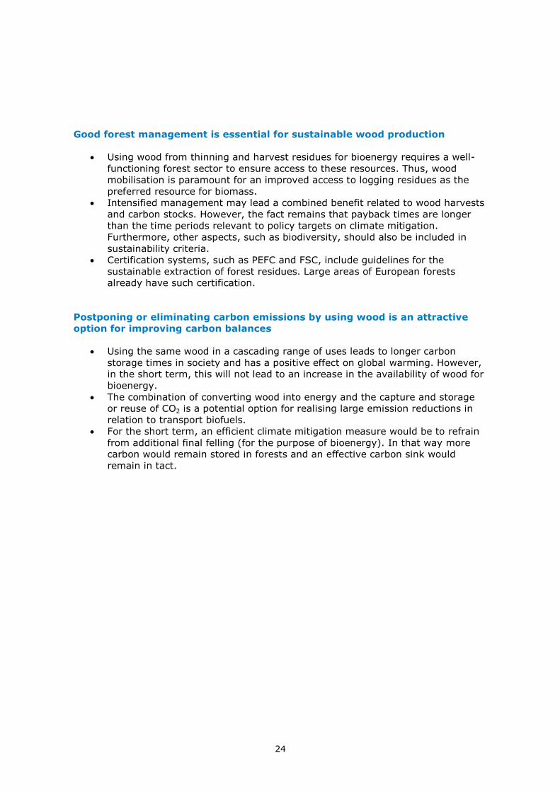
• Using the same wood in a cascading range of uses leads to longer carbon storage times in society and has a positive effect on global warming. However, in the short term, this will not lead to an increase in the availability of wood for bioenergy.

• The combination of converting wood into energy and the capture and storage or reuse of CO2 is a potential option for realising large emission reductions in relation to transport biofuels.

• For the short term, an efficient climate mitigation measure would be to refrain from additional final felling (for the purpose of bioenergy). In that way more carbon would remain stored in forests and an effective carbon sink would remain in tact.

25

References Brockerhoff E.G., Jactel H., Parrotta J.A., Quine, C.O. and.Sayer J. (2008) Plantation

forests and biodiversity: oxymoron or opportunity? Biodivers Conserv 17:925–951. DOI 10.1007/s10531-008-9380-x.

Cherubini F., Bright R.M., Strømman A.H. (2012) Site-specific global warming potentials of biogenic CO2 for bioenergy: contributions from carbon fluxes and albedo dynamics. Env. Res. Let 7:1-11. DOI: doi:10.1088/1748-9326/7/4/045902 .

Colnes, A., K. Doshi, H. Emick, A. Evans, R. Perschel, T. Robards, D. Saah and A. Sherman (2012). Biomass Supply and Carbon Accounting for Southeastern Forests, Biomass Energy Resource Center, Forest Guild, Spatial Informatics Group

Dimitriou I. & Aronsson P. (2005) Willows for energy and phytoremediation in Sweden. Unasylva 56: 47–50

EEA. (2007) Environmentally compatible bioenergy potential from European forests, European Environment Agency, Copenhagen, Denmakr. pp. 54.

Eggers, J., M. Lindner, S. Zudin, S. Zaehle, J. Liski, and G.J. Nabuurs, (2007). Forestry in Europe under changing climate and land use. Proceedings of the OECD Conference ‘Forestry: A Sectoral Response to Climate Change’, 21-23 November 2006. In: P. Freer-Smith (ed.), Forestry Commission, UK

Elbersen B., Fritsche U., Petersen J.-E., Lesschen J.P., Böttcher H., Overmars K. (2013) Assessing the effect of stricter sustainability criteria on EU biomass crop potential. Biofuels, Bioproducts and Biorefining 7:173–192. DOI: 10.1002/bbb.1407.

EUwood (2010) (Mantau, U. et al.) (2010) Real potential for changes in growth and use of EU forests. Final report. Hamburg/Germany, June 2010. 160 p

Guo LB; Gifford RM (2002). Soil carbon stocks and land use change: A meta analysis. Global Change Biology 8:345–360.

FORM (2013) Estimation of global recovery potential of degraded forest areas. Report of Form International, Hattem, the Netherlands; 54p

FAO (2010). Global Forest Resources Assessment 2010. Main report. FAO Forestry Paper No. 163. Rome., Italy, 378p, Available at: www.fao.org/docrep/013/i1757e/i1757e.pdf

Holtsmark, B. (2012). “Harvesting in boreal forests and the biofuel carbon debt.” Climatic Change 112(2): 415-428.

IEA (2013) (S.A. Lloyd & C. T. Smith). Salvage Logging and Wood Pellet Production in British Columbia: A Sustainability Assessment. IEA Bioenergy Task 43. Report 2013:02.; 25p

IINAS. (2012) Sustainability Criteria and Indicators for Solid Bioenergy from Forests, in: U. R. Fritsche, et al. (Eds.), Extending the RED Sustainability Requirements to Solid Bioenergy. pp. 109

IPCC (2003) Good Practice Guidance for Land Use, Land-Use Change and Forestry. Report IPCC National Greenhouse Gas Inventories Programme. 590p

IPCC (2007) Forestry. Chapter 9 in Climate Change 2007: Mitigation. Contribution of Working Group III to the Fourth Assessment Report of the Intergovernmental Panel on Climate Change [B. Metz, O.R. Davidson, P.R. Bosch, R. Dave, L.A. Meyer (eds)], Cambridge University Press, Cambridge, United Kingdom and New York, NY, USA., 540-584

Johnson, D.W., P.S. Curtis. 2001. Effects of forest management on soil C and N storage: meta analysis. Forest Ecology and Management 140 (2‐3):227‐238

Jonker, J.G.G., H.M. Junginger, A. Faaij (2013). “Carbon payback period and carbon offset parity point of wood pellet production in the Southeastern USA”, GCB Bioenergy DOI doi: 10.1111/gcbb.12056

26

JRC (2013) Carbon accounting of forest bioenergy. Conclusions and recommendations from a critical literature review (Eds. Agostini, Giuntoli, Boulamanti), report Joint Research Centre Technical Report nr. 25354, IPSRA, Italy, 90p

Kerr, G., Haufe, J. (2011). Thinning Practice: A Silvicultural Guide. Edinburgh: Forestry Commission. 54 pp

Koivisto, P. (1959). Growth and yield tables; communication institute Forestalis Fenniae. 51: 1-44. Finnish Forest Research Institute, Helsinki.

Lamers P., E. Thiffault, D. Paré and H.M. Junginger (2013). Feedstock specific environmental risk levels related to biomass extraction for energy from boreal and temperate forests. Biomass and Bioenergy (online early view)

Lamers P., Junginer M. (2013). The ‘debt’ is in the detail: a synthesis of recent temporal forest carbon analyses on woody biomass for energy. Biofuels, Bioproducts, and Biorefining, DOI 10.1002/bbb.1407

Lamers P., Junginer M., Dymond C. and Faaij A. (2013). “Damaged forests provide an opportunity to mitigate climate change”. GCB Bioenergy DOI 10.1111/gcbb.12055

Le Quéré C., Andres R.J., Boden T., Conway T., Houghton R.A., House J.I., Marland G., Peters G.P., van der Werf G., Ahlström A., Andrew R.M., Bopp L., Canadell J.G., Ciais P., Doney S.C., Enright C., Friedlingstein P., Huntingford C., Jain A.K., Jourdain C., Kato E., Keeling R.F., Klein Goldewijk K., Levis S., Levy P., Lomas M., Poulter B., Raupach M.R., Schwinger J., Sitch S., Stocker B.D., Viovy N., Zaehle S., Zeng N. (2013) The global carbon budget 1959–2011. Earth Syst. Sci. Data Discuss. 5:166-187. DOI: doi:10.5194/essd-5-165-2013

Lippke, B., E. Oneil, R. Harrison, K. Skog, L. Gustavsson and R. Sathre (2011). “Life cycle impacts of forest management and wood utilization on carbon mitigation: knows and unknowns.” Carbon Management 2(3): 303-333

McKechnie, J., S. Colombo, J. Chen, W. Mabee and H. L. MacLean (2011). “Forest bioenergy or forest carbon? Assessing trade-offs in greenhouse gas mitigation with wood-based fuels.” Environmental Science and Technology 45(2): 789-795.

Mitchell, S. R., M. E. Harmon and K. E. B. O’Connell (2012). “Carbon debt and carbon sequestration parity in forest bioenergy production.” GCB Bioenergy 4(6): 818-827.

MFLNRO (2012): A history of the battle against the mountain pine beetle: 2000 to 2012. Ministry of Forests, Lands and Natural Resources Operations. Available at www.for.gov.bc.ca/hfp/mountain_pine_beetle/Pine%20Beetle%20Response%20Brief%20History%20May%2023%202012.pdf

Niquidet K., Stennes B., and van Kooten, G.C. (2012) Bioenergy from Mountain Pine Beetle Timber and Forest Residuals: A Cost Analysis. Canadian Journal of Agricultural Economics 60:195-210. DOI: 10.1111/j.1744-7976.2012.01246.x

ProBos (2009) (M. Boosten, J. Oldenburger, J. Oorschot, M. Boertjes & J. van den Briel) De logistieke keten van houtige biomassa uit bos, natuur en landschap in Nederland: stand van zaken, knelpunten en kansen. Report Probos Foundation, Wageningen, the Netherlands, 94 p

Repo, A., Känkänen R., Tuovinen J.-P., Antikainen R., Tuomi M., Vanhala P., and Liski J. (2012). “Forest bioenergy climate impact can be improved by allocating forest residue removal.” GCB Bioenergy 4(2): 202-212.

Sathre, R. and Gustavsson L. (2011). “Time-dependent climate benefits of using forest residues to substitute fossil fuels.” Biomass and Bioenergy 35(7): 2506- 2516.

Sathre, R. and J. O’Connor (2010). Meta-analysis of greenhouse gas displacement factors of wood product substitution. Environmental Science and Policy 13 (2010) 104-114.

Schuck, A.; Meyer, P.; Menke, N.; Lier, M. & Lindner, M. (2004). Forest biodiversity indicator: dead wood - a proposed approach towards operationalising the MCPFE indicator. EFI-Proceedings, Vol. 51, 49-77

Thornley J.H.M., Cannell M.G.R. (2000) Managing forests for wood yield and carbon storage: a theoretical study. Tree Physiology 20:477–484.

27

Trømborg E., Sjølie H. K., Bergseng E., Bolkesjø T. F., Hofstad O., Rørstad P., K., Solberg B., Sunde K. (2011). ”Carbon cycle effects of different strategies for utilisation of forest resources – a review”, INA fagrapport 19, Norwegian University of Life Sciences.

Tsarev A.P. (2005). Natural poplar and willow ecosystems on a grand scale: the Russian Federation. Unasylva 55: 10-11

UNFCCC (2007) "Kyoto Protocol." United Nations Framework Convention on Climate Change. Web. 26 Nov. 2009. http://www.unfccc.int .

Werner C., Haas E., Grote R., Gauder M., Graeff-Hönninger S., Claupein W., Butterbach-Bahl K. (2012) Biomass production potential from Populus short rotation systems in Romania. GCB Bioenergy 4:642-653. DOI: 10.1111/j.1757-1707.2012.01180.x.

Zanchi, G., N. Pena and N. Bird (2012). “Is woody bioenergy carbon neutral? A comparative assessment of emissions from consumption of woody bioenergy and fossil fuel.” GCB Bioenergy 4(6): 761-772

28

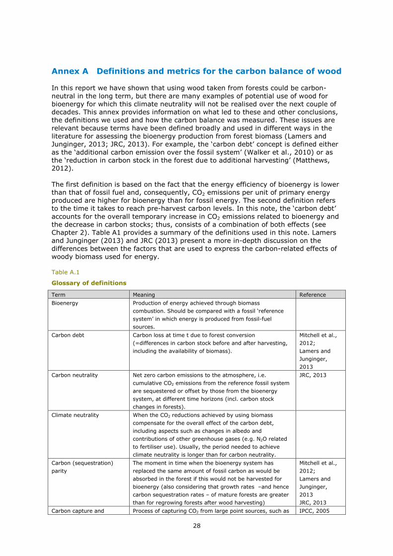
Annex A Definitions and metrics for the carbon balance of wood In this report we have shown that using wood taken from forests could be carbon-neutral in the long term, but there are many examples of potential use of wood for bioenergy for which this climate neutrality will not be realised over the next couple of decades. This annex provides information on what led to these and other conclusions, the definitions we used and how the carbon balance was measured. These issues are relevant because terms have been defined broadly and used in different ways in the literature for assessing the bioenergy production from forest biomass (Lamers and Junginger, 2013; JRC, 2013). For example, the ‘carbon debt’ concept is defined either as the ‘additional carbon emission over the fossil system’ (Walker et al., 2010) or as the ‘reduction in carbon stock in the forest due to additional harvesting’ (Matthews, 2012). The first definition is based on the fact that the energy efficiency of bioenergy is lower than that of fossil fuel and, consequently, CO2 emissions per unit of primary energy produced are higher for bioenergy than for fossil energy. The second definition refers to the time it takes to reach pre-harvest carbon levels. In this note, the ‘carbon debt’ accounts for the overall temporary increase in CO2 emissions related to bioenergy and the decrease in carbon stocks; thus, consists of a combination of both effects (see Chapter 2). Table A1 provides a summary of the definitions used in this note. Lamers and Junginger (2013) and JRC (2013) present a more in-depth discussion on the differences between the factors that are used to express the carbon-related effects of woody biomass used for energy. Table A.1

Glossary of definitions

Term Meaning Reference Bioenergy Production of energy achieved through biomass

combustion. Should be compared with a fossil ‘reference system’ in which energy is produced from fossil-fuel sources.

Carbon debt Carbon loss at time t due to forest conversion (=differences in carbon stock before and after harvesting, including the availability of biomass).

Mitchell et al., 2012; Lamers and Junginger, 2013

Carbon neutrality Net zero carbon emissions to the atmosphere, i.e. cumulative CO2 emissions from the reference fossil system are sequestered or offset by those from the bioenergy system, at different time horizons (incl. carbon stock changes in forests).

JRC, 2013

Climate neutrality When the CO2 reductions achieved by using biomass compensate for the overall effect of the carbon debt, including aspects such as changes in albedo and contributions of other greenhouse gases (e.g. N2O related to fertiliser use). Usually, the period needed to achieve climate neutrality is longer than for carbon neutrality.

Carbon (sequestration) parity

The moment in time when the bioenergy system has replaced the same amount of fossil carbon as would be absorbed in the forest if this would not be harvested for bioenergy (also considering that growth rates –and hence carbon sequestration rates – of mature forests are greater than for regrowing forests after wood harvesting)

Mitchell et al., 2012; Lamers and Junginger, 2013 JRC, 2013

Carbon capture and Process of capturing CO2 from large point sources, such as IPCC, 2005

29

storage (CCS) power plants, transporting and storing it where it will not enter the atmosphere (normally in underground geological formations).

Displacement factor Ratio between the efficiency (here in terms of CO2 emissions) of the use of biomass and that of alternative sources (often fossil fuel)

Sathre and O’Connor, 2010

Emission factor Ratio between the amount of CO2 generated and the outputs from production processes

OECD, 2001

Forest management Stewardship and use of forest land, mainly to increase productivity and timber quality, and maintain other (economic and ecological) services

IEA, 2013; JRC, 2013

Fossil fuel parity The moment that the amount of CO2 emitted into the atmosphere from a bioenergy system and the fossil-fuel reference are the same

JRC, 2013

Harvest residue Wood usually left in the forest after harvesting or thinning (e.g. tops, stumps, branches, foliage, roots).

JRC, 2013

Payback time Time span within which carbon parity is reached JRC, 2013 Thinning Common silvicultural practice in forest management, in

which certain trees are selectively removed. Main objective is to improve stand quality and to generate intermediate economic returns

Kerr and Haufe, 2011; IINAS,2012

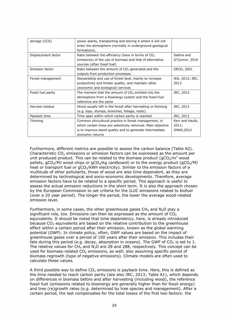
Furthermore, different metrics are possible to assess the carbon balance (Table A2). Characteristic CO2 emissions or emission factors can be expressed as the amount per unit produced product. This can be related to the biomass product (gCO2/m3 wood pellets, gCO2/MJ wood chips or gCO2/kg cardboard) or to the energy product (gCO2/MJ heat or transport fuel or gCO2/kWh electricity). Similar to the emission factors of a multitude of other pollutants, those of wood are also time dependent, as they are determined by technological and socio-economic developments. Therefore, average emission factors have to be related to a specific period. This approach is useful to assess the actual emission reductions in the short term. It is also the approach chosen by the European Commission to set criteria for the ILUC emissions related to biofuel (over a 20 year period). The longer the period, the lower the average wood-related emission level. Furthermore, in some cases, the other greenhouse gases CH4 and N2O play a significant role, too. Emissions can then be expressed as the amount of CO2 equivalents. It should be noted that time dependency, here, is already introduced because CO2 equivalents are based on the relative contribution to the greenhouse effect within a certain period after their emission, known as the global warming potential (GWP). In climate policy, often, GWP values are based on the impact of greenhouse gases over a period of 100 years after their emission. This includes their fate during this period (e.g. decay, absorption in oceans). The GWP of CO2 is set to 1. The relative values for CH4 and N2O are 28 and 288, respectively. This concept can be used for biomass-related CO2 emissions, as well; also assuming specific period of biomass regrowth (type of negative emissions). Climate models are often used to calculate these values. A third possible way to define CO2 emissions is payback time. Here, this is defined as the time needed to reach carbon parity (see also JRC, 2013; Table A1), which depends on differences in biomass before and after harvesting (including wood), the reference fossil fuel (emissions related to bioenergy are generally higher than for fossil energy) and tree (re)growth rates (e.g. determined by tree species and management). After a certain period, the last compensates for the total losses of the first two factors: the

30

payback period. Thus, the payback time not only depends on historical developments in the forest, but also on future growth rate (JRC, 2013). Table A.2

Survey of metrics for the carbon balance of wood

Metrics Explanation Average emission factors of wood and bioenergy

gCO2/MJ wood, or gCO2/m3 wood

A. The total of the net bioenergy-related emissions in a certain period, including emissions forest management, harvesting, transport and pre-treatment

gCO2/MJ (fuel or heat), or gCO2/kWh

B. The same emissions as for A, but also including the efficiency and any additional fossil emissions following the conversion

GWP Relative factor (CO2=1 for fossil emissions)

Greenhouse Warming Potential over a certain period (mostly 100 years); it simulates the temperature rise over this period, after a pulse emission of a specific gas, using model calculations, including the behaviour of the gas within the ecosystem and adding the specific uptake by a similar type of biomass

Carbon parity factor

Dimensionless factor (this study)

Ratio (the carbon emissions related to bioenergy, minus the carbon uptake

in the forest) divided by

(the carbon emissions in the alternative system (mostly fossil energy),

minus the carbon uptake in the same forest without harvesting)

Payback time

Years

Period in which the greenhouse gas emissions related to bioenergy minus the CO2 uptake in the forest due to biomass regrowth equals the greenhouse gas emissions in the alternative system (mostly fossil energy)

31

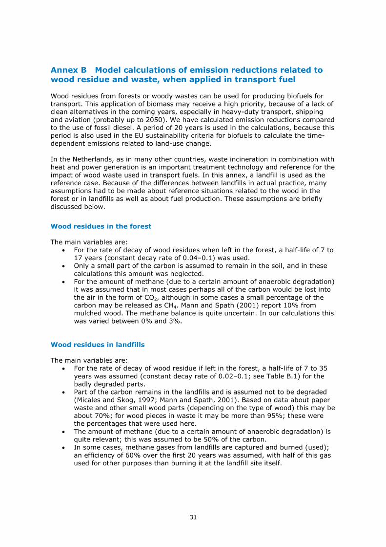
Annex B Model calculations of emission reductions related to wood residue and waste, when applied in transport fuel Wood residues from forests or woody wastes can be used for producing biofuels for transport. This application of biomass may receive a high priority, because of a lack of clean alternatives in the coming years, especially in heavy-duty transport, shipping and aviation (probably up to 2050). We have calculated emission reductions compared to the use of fossil diesel. A period of 20 years is used in the calculations, because this period is also used in the EU sustainability criteria for biofuels to calculate the time-dependent emissions related to land-use change. In the Netherlands, as in many other countries, waste incineration in combination with heat and power generation is an important treatment technology and reference for the impact of wood waste used in transport fuels. In this annex, a landfill is used as the reference case. Because of the differences between landfills in actual practice, many assumptions had to be made about reference situations related to the wood in the forest or in landfills as well as about fuel production. These assumptions are briefly discussed below.

Wood residues in the forest

The main variables are: • For the rate of decay of wood residues when left in the forest, a half-life of 7 to

17 years (constant decay rate of 0.04–0.1) was used. • Only a small part of the carbon is assumed to remain in the soil, and in these

calculations this amount was neglected. • For the amount of methane (due to a certain amount of anaerobic degradation)

it was assumed that in most cases perhaps all of the carbon would be lost into the air in the form of CO2, although in some cases a small percentage of the carbon may be released as CH4. Mann and Spath (2001) report 10% from mulched wood. The methane balance is quite uncertain. In our calculations this was varied between 0% and 3%.

Wood residues in landfills

The main variables are: • For the rate of decay of wood residue if left in the forest, a half-life of 7 to 35

years was assumed (constant decay rate of 0.02–0.1; see Table B.1) for the badly degraded parts.

• Part of the carbon remains in the landfills and is assumed not to be degraded (Micales and Skog, 1997; Mann and Spath, 2001). Based on data about paper waste and other small wood parts (depending on the type of wood) this may be about 70%; for wood pieces in waste it may be more than 95%; these were the percentages that were used here.

• The amount of methane (due to a certain amount of anaerobic degradation) is quite relevant; this was assumed to be 50% of the carbon.

• In some cases, methane gases from landfills are captured and burned (used); an efficiency of 60% over the first 20 years was assumed, with half of this gas used for other purposes than burning it at the landfill site itself.

32

Table B.1

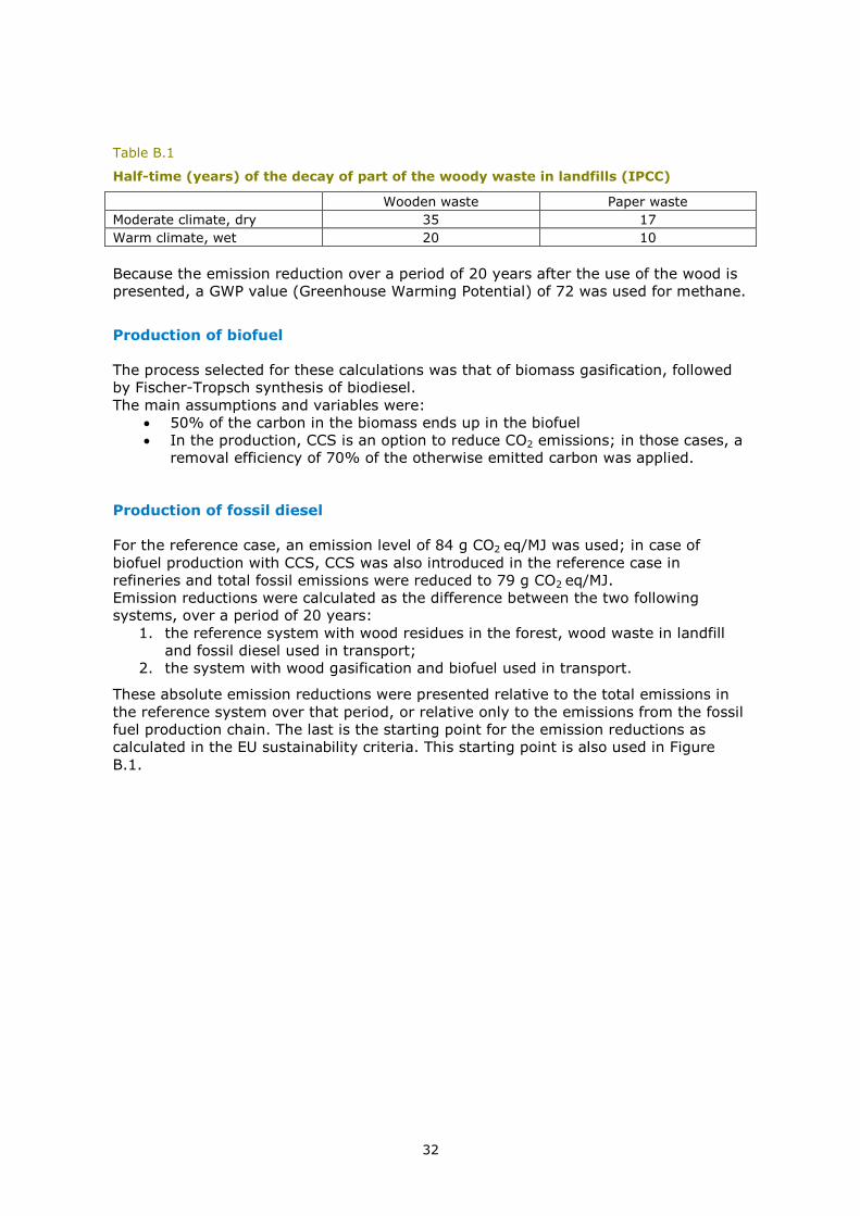
Half-time (years) of the decay of part of the woody waste in landfills (IPCC)

Wooden waste Paper waste Moderate climate, dry 35 17 Warm climate, wet 20 10 Because the emission reduction over a period of 20 years after the use of the wood is presented, a GWP value (Greenhouse Warming Potential) of 72 was used for methane.

Production of biofuel

The process selected for these calculations was that of biomass gasification, followed by Fischer-Tropsch synthesis of biodiesel. The main assumptions and variables were:

• 50% of the carbon in the biomass ends up in the biofuel • In the production, CCS is an option to reduce CO2 emissions; in those cases, a

removal efficiency of 70% of the otherwise emitted carbon was applied.

Production of fossil diesel

For the reference case, an emission level of 84 g CO2 eq/MJ was used; in case of biofuel production with CCS, CCS was also introduced in the reference case in refineries and total fossil emissions were reduced to 79 g CO2 eq/MJ. Emission reductions were calculated as the difference between the two following systems, over a period of 20 years:

1. the reference system with wood residues in the forest, wood waste in landfill and fossil diesel used in transport;

2. the system with wood gasification and biofuel used in transport.

These absolute emission reductions were presented relative to the total emissions in the reference system over that period, or relative only to the emissions from the fossil fuel production chain. The last is the starting point for the emission reductions as calculated in the EU sustainability criteria. This starting point is also used in Figure B.1.

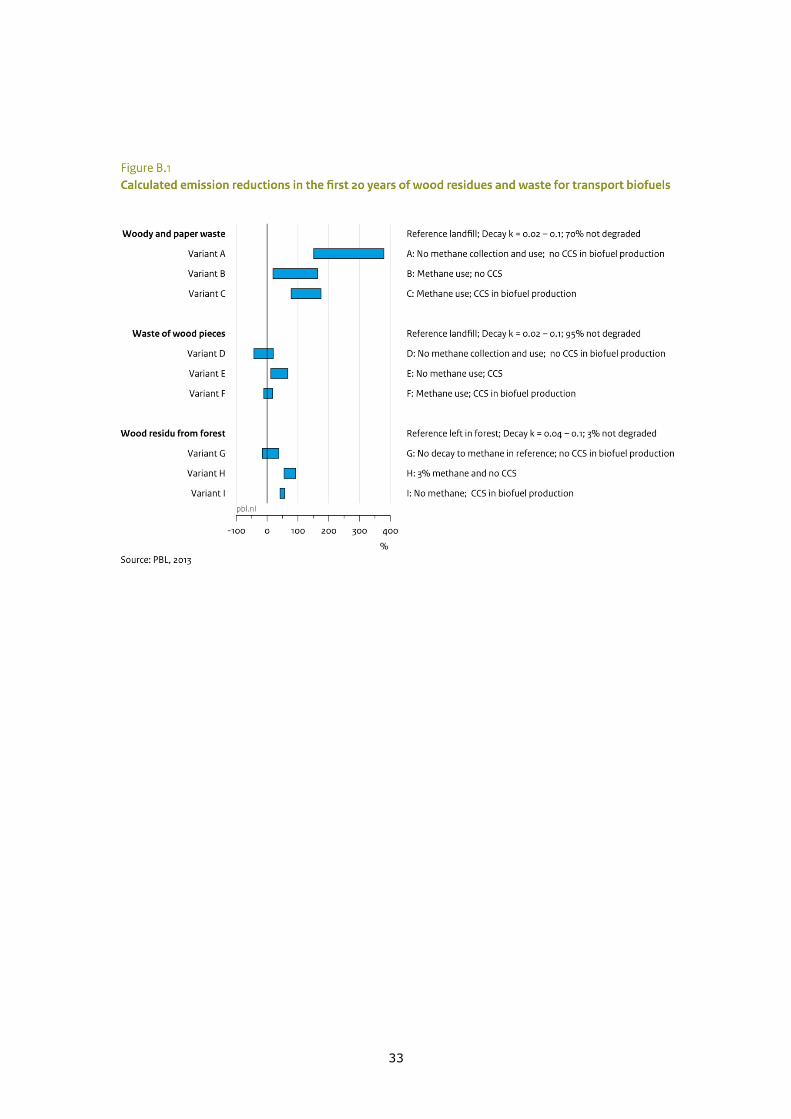
33

34

Annex C Carbon dynamics for different types of European forests, using EFISCEN model calculations

Introduction Currently, most of the wood used for industrial-scale bioenergy applications in the Netherlands is imported in the form of wood pellets made from sawing residues or residue from salvage logging of beetle-infested forests in Canada (Lamers et al., 2013), while only a small amount of wood for bioenergy purposes comes from primary wood sources. Yet, as indicated in several econometric studies, with the strongly increasing demand for wood for bioenergy purposes and its effects on wood prices, it is not entirely unimaginable that this will not happen in the future (e.g. Buongiorno et al., 2011; Moiseyev et al., 2011; Raunikar et al., 2010). Whether primary wood sources eventually will be used on a large scale will largely depend on timber and paper price developments, subsidy levels for woody biomass used in bioenergy applications, and provisions in sustainability criteria for using woody biomass for bioenergy (e.g. Moiseyev et al., 2011). Using the EFISCEN 3.2 model, we assessed the carbon impact of increasing the demand for woody biomass – in this case, for using it as biofuel in electricity generation. The model makes large-scale projections based on current age class distribution and biomass increments and mortality functions, as derived from national forest inventories in Europe. Objective of this modelling experiment was to increase the insight into the total carbon balance if additional wood for bioenergy would be sourced from forests in different ways. We included additional sourcing of round wood from final felling, wood from intermediate thinning, as well as an increase in the use of woody harvest residues. We applied this to 8 types of forests across Europe that differed in terms of species, growing conditions and management, and were considered to cover the full range of growth and management systems in Europe. We chose European forests for this modelling experiment because of model and data availability. However, similar principles would apply to other temperate and boreal regions, with forests characterised by an age distribution towards relatively young mature forests that still act as a net carbon sink, such as in large parts of the forests in the United States. The ‘what if’ types of scenarios with increased sourcing of wood were compared to a reference level with approximately current wood harvesting levels, and were used to obtain a better understanding of the factors underlying potential carbon debts if wood is used for bioenergy. This information may be used in bioenergy policy development and supports the development of sustainability criteria for woody biomass used for bioenergy.

European forests European forests have been a central land-forming and resource-delivering element since the beginning of human settlement. Although heavily exploited in earlier times, forest resources currently prosper; forest in Europe covered around 37% of the land in 2010, and forest area and growing stock increased by 8% between 1990 and 2010. The forest area, however, also has been affected by afforestation, natural reforestation, and larger stocks due to an increase in annual increments that also are not fully harvested (62% of increments were harvested in 2010). This wealth of resources is subject to very different forest management regimes, methods of land-use planning and policy-making. Forests are very heterogeneous, in terms of forest type, and are unequally distributed across Europe (see Figure C.1). Because of current under-harvesting, European

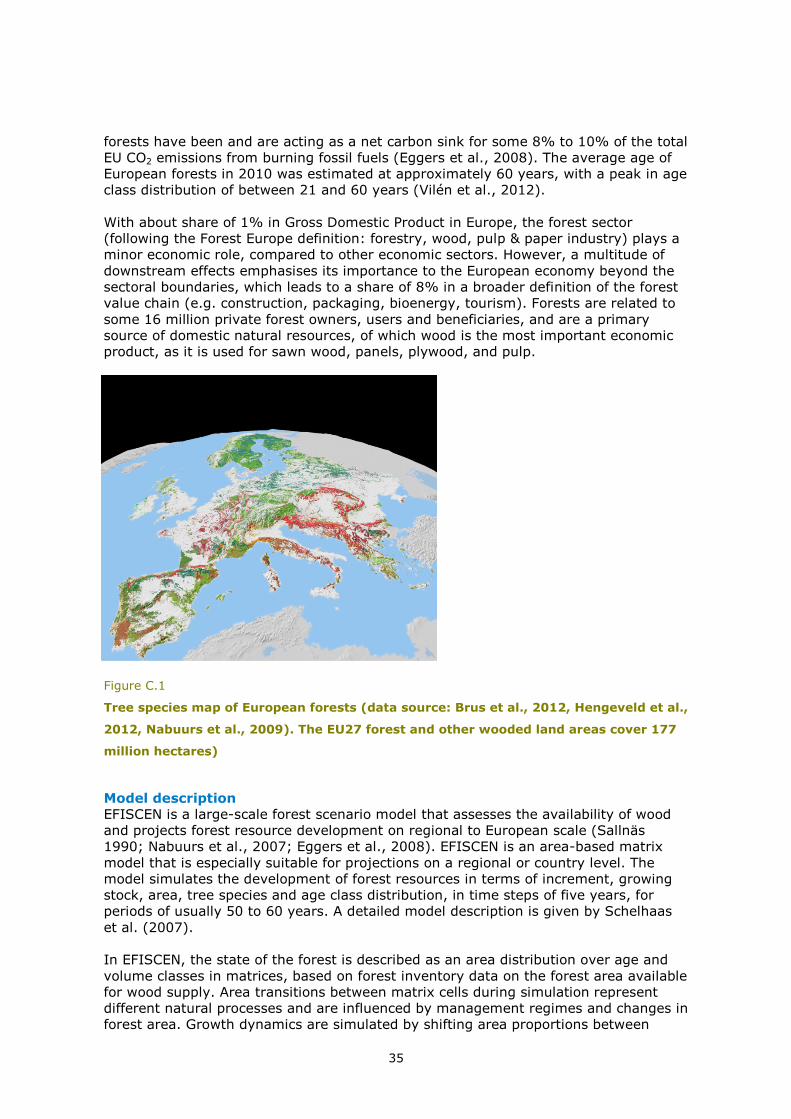
35

forests have been and are acting as a net carbon sink for some 8% to 10% of the total EU CO2 emissions from burning fossil fuels (Eggers et al., 2008). The average age of European forests in 2010 was estimated at approximately 60 years, with a peak in age class distribution of between 21 and 60 years (Vilén et al., 2012). With about share of 1% in Gross Domestic Product in Europe, the forest sector (following the Forest Europe definition: forestry, wood, pulp & paper industry) plays a minor economic role, compared to other economic sectors. However, a multitude of downstream effects emphasises its importance to the European economy beyond the sectoral boundaries, which leads to a share of 8% in a broader definition of the forest value chain (e.g. construction, packaging, bioenergy, tourism). Forests are related to some 16 million private forest owners, users and beneficiaries, and are a primary source of domestic natural resources, of which wood is the most important economic product, as it is used for sawn wood, panels, plywood, and pulp.

Figure C.1

Tree species map of European forests (data source: Brus et al., 2012, Hengeveld et al.,

2012, Nabuurs et al., 2009). The EU27 forest and other wooded land areas cover 177

million hectares)

Model description EFISCEN is a large-scale forest scenario model that assesses the availability of wood and projects forest resource development on regional to European scale (Sallnäs 1990; Nabuurs et al., 2007; Eggers et al., 2008). EFISCEN is an area-based matrix model that is especially suitable for projections on a regional or country level. The model simulates the development of forest resources in terms of increment, growing stock, area, tree species and age class distribution, in time steps of five years, for periods of usually 50 to 60 years. A detailed model description is given by Schelhaas et al. (2007). In EFISCEN, the state of the forest is described as an area distribution over age and volume classes in matrices, based on forest inventory data on the forest area available for wood supply. Area transitions between matrix cells during simulation represent different natural processes and are influenced by management regimes and changes in forest area. Growth dynamics are simulated by shifting area proportions between

36

matrix cells. In each 5-year time step, the area in each matrix cell moves up one age class to simulate ageing. Part of the area of a cell also moves to a higher volume class, thereby simulating volume increment. Growth dynamics are estimated by the model’s growth functions whose coefficients are based on inventory data or yield tables. Management is specified at two levels in the model. Firstly, a basic management regime defines the period during which thinning may take place and a minimum age for final felling. These regimes can be regarded as constraints on the total harvest level. Thinning is implemented by moving an area to a lower volume class. Final felling is implemented by moving an area outside the matrix to a bare-forest-land class, from where it can re-enter the matrix and thereby reflect forest regeneration. Secondly, the demand for wood is specified for thinning and for final felling, separately, and EFISCEN fells the required wood volume, if available. To assess biomass in branches, coarse roots, fine roots and foliage, stemwood volumes are converted to stem biomass by using basic wood density (dry weight per green volume) and to whole-tree biomass using age- and species-specific biomass allocation functions. For carbon, a carbon content of 50% is used. During thinning and final felling harvest residues are formed. These residues consist of stemwood harvest losses (e.g. stem tops), as well as branches and foliage that are separated from the harvested trees. In addition to these harvest residues, there will be dead stumps and dead coarse roots In the model, it is possible to define which share of the residues and stumps/coarse roots are removed from the forest during thinning and final felling. Residues and stumps/roots that are left in the forest will eventually decay, as they become part of the soil module. EFISCEN does not have a wood products module, all harvested wood is assumed to be an emission source of carbon in the same year, except the residues that stay in the forest and decay there. Therefore, the net carbon balance of additional sourcing of wood for bioenergy is calculated in a spreadsheet, including the different forest carbon pools as provided by EFISCEN and all the carbon in the wood harvested since the start of the additional harvesting. The effect of different displacement factors is also assessed in this spread sheet.

Scenarios Here, eight different types of forests across Europe with contrasting growth and management characteristics (Table C.1) were used to assess the impact of increased wood harvesting on total carbon dynamics, the potential of woody biomass from different sources to offset carbon emissions from fossil fuels, and the time needed to reach carbon parity compared to a situation without additional wood harvesting for bioenergy. On a regional level, the EFISCEN model was applied for the eight forest types covering the growth range of systems in Europe. These systems were used as concrete examples to elaborate the effects of increased wood demand on carbon dynamics in European forests. The model runs cover the total area that these species occupy in the selected countries (see Table C.1). Situations to assess in different scenarios:

1. Reference scenario, giving the carbon emissions and carbon sink for the specified forest type and region (based on the EFSOS II B2 baseline scenario, for more details see UNECE/FAO 2012), including reference harvesting levels, but excluding afforestation, reforestation and deforestation. This does not include the removal of harvest residues.

37

2. Moderate level of additional harvesting of round wood for the production of biomass (energy). Increasing total harvests from final felling by 10%, no additional harvest from thinning and no change in the use of harvest residues.

3. High level additional harvest of round wood for the production of biomass (energy). Increasing total harvests from final felling by 50%, no additional harvest from thinning and no change in the use of harvest residues.

4. Moderate level of additional thinning of round wood for the production of biomass (energy). Increasing total harvests from thinning by 10%, no additional harvest from final felling and no change in the use of harvest residues.

5. High level of additional thinning of round wood for the production of biomass (energy). Increasing total harvests from thinning by 50%, no additional harvest from final felling and no change in the use of harvest residues.

6. No additional harvest of round wood compared to the baseline, but 50% of harvest residues are removed for bioenergy

7. No additional harvest of round wood compared to the baseline, but 100% of harvest residues are removed for bioenergy.

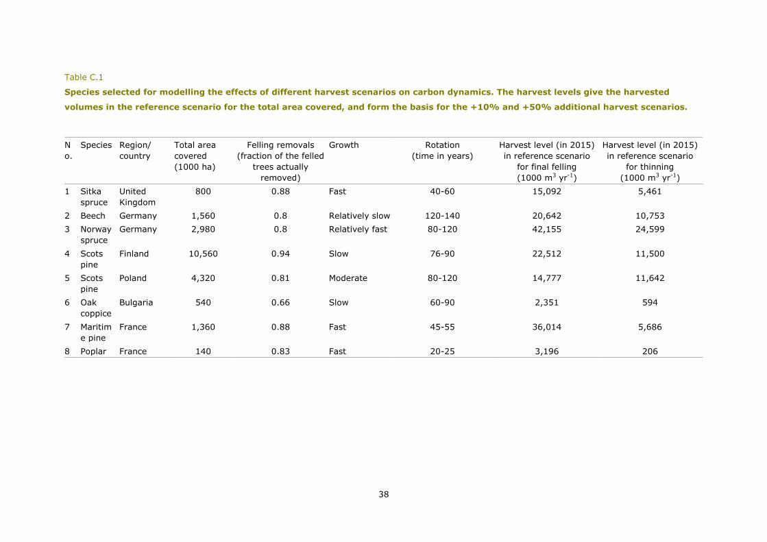
38

Table C.1

Species selected for modelling the effects of different harvest scenarios on carbon dynamics. The harvest levels give the harvested

volumes in the reference scenario for the total area covered, and form the basis for the +10% and +50% additional harvest scenarios.

No.

Species Region/ country

Total area covered (1000 ha)

Felling removals (fraction of the felled

trees actually removed)

Growth Rotation (time in years)

Harvest level (in 2015) in reference scenario

for final felling (1000 m3 yr-1)

Harvest level (in 2015) in reference scenario

for thinning (1000 m3 yr-1)

1 Sitka spruce

United Kingdom

800 0.88 Fast 40-60 15,092 5,461

2 Beech Germany 1,560 0.8 Relatively slow 120-140 20,642 10,753 3 Norway

spruce Germany 2,980 0.8 Relatively fast 80-120 42,155 24,599

4 Scots pine

Finland 10,560 0.94 Slow 76-90 22,512 11,500

5 Scots pine

Poland 4,320 0.81 Moderate 80-120 14,777 11,642

6 Oak coppice

Bulgaria 540 0.66 Slow 60-90 2,351 594

7 Maritime pine

France 1,360 0.88 Fast 45-55 36,014 5,686

8 Poplar France 140 0.83 Fast 20-25 3,196 206

39

First, for each combination of species and country used in the scenarios, the reference levels of harvesting from final felling and thinning by 2015 (see Table C.1) were assessed using the EFSOS II B2 baseline scenario settings for the model. These settings included, per country, an overall demand for wood from final felling and thinning without specification of this demand across the tree species. Based on the availability of the forest area that can be harvested, the model distributes the demand over the species and regions per country. This does not necessarily accurately reflect current harvesting levels for those tree species. In some cases, these reference harvesting levels could not be maintained over longer periods of time, because of a temporary unavailability of forest stands old enough to be harvested. As a result, initial overharvesting will then result, reducing harvest levels in subsequent years, which, for the purpose of this modelling experiment, results in an undesired feedback that would make comparison among scenarios not very meaningful. Therefore, for countries (i.e. Finland and Germany) for which it was not possible to maintain these reference levels or increased harvesting levels over the first 50 years, the reference harvesting levels were reduced to a level that could be maintained over a longer period of time. Using (close to) current levels of harvesting as a reference ensured that forests would not become much older than the oldest forest available in the underlying forest inventories. Most forests will not reach a state with highly increased mortality

Carbon debt metrics calculated Based on the EFISCEN model outputs for the different scenarios, two different yet related metrics were calculated to assess the carbon benefit/debit effect of increasing harvesting of wood for bioenergy production.

Carbon parity Carbon parity is reached when the difference in carbon in the forest system between the reference scenario and the additional sourcing scenario is balanced by the carbon offset. C parity in year t = C (in forest of reference scenario in year t) – C(in forest of scenario in year t) – (C(in wood

removed for bioenergy up until year t) * displacement factor) The model provides output on total carbon in the different carbon pools in the forest system (living biomass, standing dead wood, soil including different litter fractions). These pools were combined to provide the total amount of carbon in the ecosystem. The replacement factor gives information on the effect on emission levels from substituting fossil fuels with wood. This takes into consideration the difference in CO2 emissions per unit of primary energy produced, differences in efficiency of energy conversion (e.g. the conversion from primary energy to electricity) and in some cases differences in emissions along the chain from harvesting to being used in power plants. The replacement factors provided in other studies vary strongly and depend on many factors, such as the type of wood used and the efficiency level of the power plant. Therefore, here, three contrasting replacement factors were estimated: 1 (assumes emissions from burning wood are similar to those from fossil fuels), 0.63 substituting coal with wood and 0.3 for substituting natural gas. The focus of this case study was not on assessing an accurate value for the various replacement factors, as these are very uncertain and power plant-specific. Here, these factors were used to show the range in potential effects.

Carbon offset parity factor The carbon offset factor gives the amount of carbon loss in the forest ecosystem, including carbon in the harvested wood, in relation to the amount of carbon emission prevented by offsetting fossil fuel emissions. This factor indicates how, under

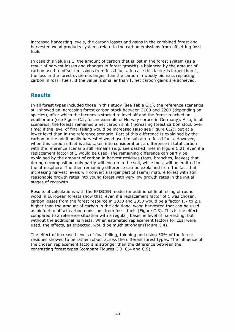
40

increased harvesting levels, the carbon losses and gains in the combined forest and harvested wood products systems relate to the carbon emissions from offsetting fossil fuels. In case this value is 1, the amount of carbon that is lost in the forest system (as a result of harvest losses and changes in forest growth) is balanced by the amount of carbon used to offset emissions from fossil fuels. In case this factor is larger than 1, the loss in the forest system is larger than the carbon in woody biomass replacing carbon in fossil fuels. If the value is smaller than 1, net carbon gains are achieved.

Results In all forest types included those in this study (see Table C.1), the reference scenarios still showed an increasing forest carbon stock between 2100 and 2200 (depending on species), after which the increases started to level off and the forest reached an equilibrium (see Figure C.2, for an example of Norway spruce in Germany). Also, in all scenarios, the forests remained a net carbon sink (increasing forest carbon stock over time) if the level of final felling would be increased (also see Figure C.2), but at a lower level than in the reference scenario. Part of this difference is explained by the carbon in the additionally harvested wood used to substitute fossil fuels. However, when this carbon offset is also taken into consideration, a difference in total carbon with the reference scenario still remains (e.g. see dashed lines in Figure C.2), even if a replacement factor of 1 would be used. The remaining difference can partly be explained by the amount of carbon in harvest residues (tops, branches, leaves) that during decomposition only partly will end up in the soil, while most will be emitted to the atmosphere. The then remaining difference can be explained from the fact that increasing harvest levels will convert a larger part of (semi) mature forest with still reasonable growth rates into young forest with very low growth rates in the initial stages of regrowth. Results of calculations with the EFISCEN model for additional final felling of round wood in European forests show that, even if a replacement factor of 1 was chosen, carbon losses from the forest resource in 2030 and 2050 would be a factor 1.7 to 2.1 higher than the amount of carbon in the additional wood harvested that can be used as biofuel to offset carbon emissions from fossil fuels (Figure C.3). This is the effect compared to a reference situation with a regular, baseline level of harvesting, but without the additional harvests. When estimated replacement factors for coal were used, the effects, as expected, would be much stronger (Figure C.4). The effect of increased levels of final felling, thinning and using 50% of the forest residues showed to be rather robust across the different forest types. The influence of the chosen replacement factors is stronger than the difference between the contrasting forest types (compare Figures C.3, C.4 and C.9).

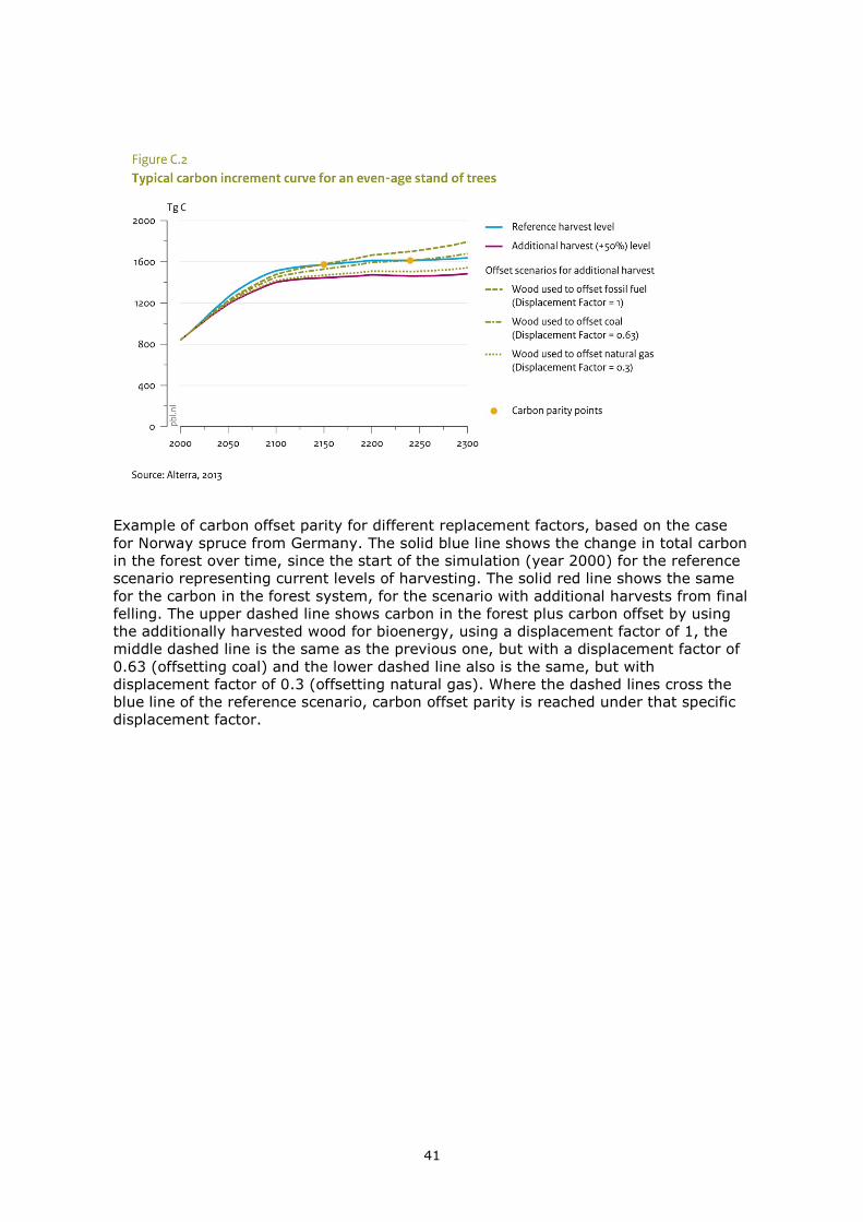
41

Example of carbon offset parity for different replacement factors, based on the case for Norway spruce from Germany. The solid blue line shows the change in total carbon in the forest over time, since the start of the simulation (year 2000) for the reference scenario representing current levels of harvesting. The solid red line shows the same for the carbon in the forest system, for the scenario with additional harvests from final felling. The upper dashed line shows carbon in the forest plus carbon offset by using the additionally harvested wood for bioenergy, using a displacement factor of 1, the middle dashed line is the same as the previous one, but with a displacement factor of 0.63 (offsetting coal) and the lower dashed line also is the same, but with displacement factor of 0.3 (offsetting natural gas). Where the dashed lines cross the blue line of the reference scenario, carbon offset parity is reached under that specific displacement factor.

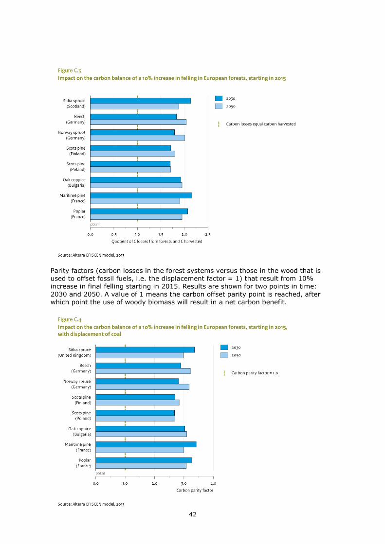
42

Parity factors (carbon losses in the forest systems versus those in the wood that is used to offset fossil fuels, i.e. the displacement factor = 1) that result from 10% increase in final felling starting in 2015. Results are shown for two points in time: 2030 and 2050. A value of 1 means the carbon offset parity point is reached, after which point the use of woody biomass will result in a net carbon benefit.

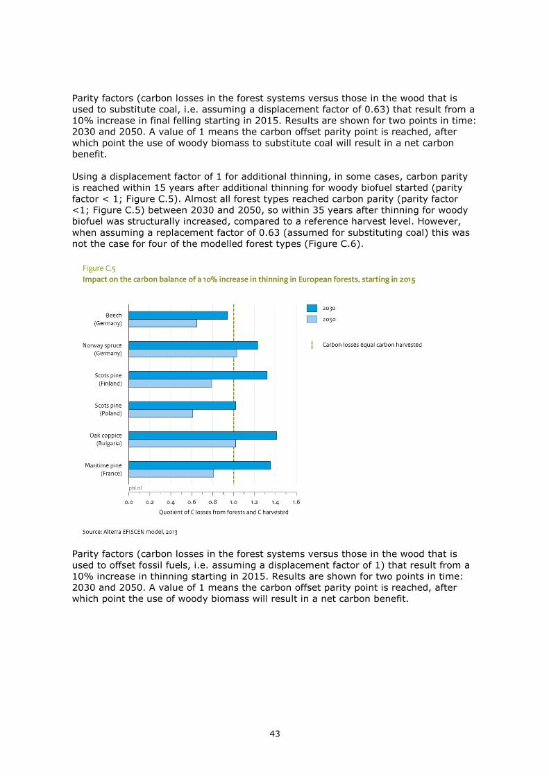
43

Parity factors (carbon losses in the forest systems versus those in the wood that is used to substitute coal, i.e. assuming a displacement factor of 0.63) that result from a 10% increase in final felling starting in 2015. Results are shown for two points in time: 2030 and 2050. A value of 1 means the carbon offset parity point is reached, after which point the use of woody biomass to substitute coal will result in a net carbon benefit. Using a displacement factor of 1 for additional thinning, in some cases, carbon parity is reached within 15 years after additional thinning for woody biofuel started (parity factor < 1; Figure C.5). Almost all forest types reached carbon parity (parity factor <1; Figure C.5) between 2030 and 2050, so within 35 years after thinning for woody biofuel was structurally increased, compared to a reference harvest level. However, when assuming a replacement factor of 0.63 (assumed for substituting coal) this was not the case for four of the modelled forest types (Figure C.6).

Parity factors (carbon losses in the forest systems versus those in the wood that is used to offset fossil fuels, i.e. assuming a displacement factor of 1) that result from a 10% increase in thinning starting in 2015. Results are shown for two points in time: 2030 and 2050. A value of 1 means the carbon offset parity point is reached, after which point the use of woody biomass will result in a net carbon benefit.

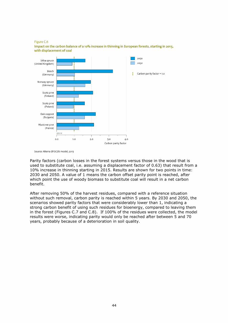
44

Parity factors (carbon losses in the forest systems versus those in the wood that is used to substitute coal, i.e. assuming a displacement factor of 0.63) that result from a 10% increase in thinning starting in 2015. Results are shown for two points in time: 2030 and 2050. A value of 1 means the carbon offset parity point is reached, after which point the use of woody biomass to substitute coal will result in a net carbon benefit. After removing 50% of the harvest residues, compared with a reference situation without such removal, carbon parity is reached within 5 years. By 2030 and 2050, the scenarios showed parity factors that were considerably lower than 1, indicating a strong carbon benefit of using such residues for bioenergy, compared to leaving them in the forest (Figures C.7 and C.8). If 100% of the residues were collected, the model results were worse, indicating parity would only be reached after between 5 and 70 years, probably because of a deterioration in soil quality.

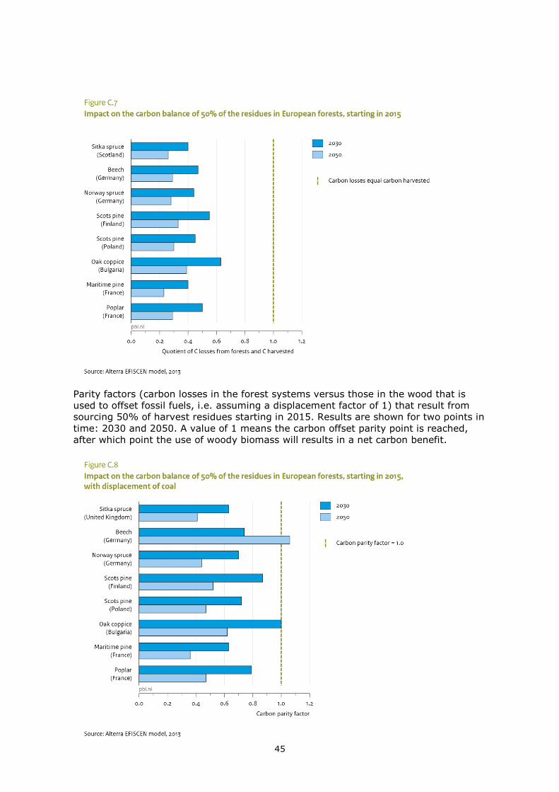
45

Parity factors (carbon losses in the forest systems versus those in the wood that is used to offset fossil fuels, i.e. assuming a displacement factor of 1) that result from sourcing 50% of harvest residues starting in 2015. Results are shown for two points in time: 2030 and 2050. A value of 1 means the carbon offset parity point is reached, after which point the use of woody biomass will results in a net carbon benefit.

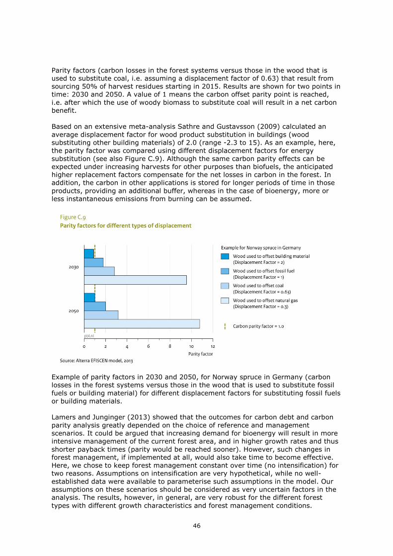
46

Parity factors (carbon losses in the forest systems versus those in the wood that is used to substitute coal, i.e. assuming a displacement factor of 0.63) that result from sourcing 50% of harvest residues starting in 2015. Results are shown for two points in time: 2030 and 2050. A value of 1 means the carbon offset parity point is reached, i.e. after which the use of woody biomass to substitute coal will result in a net carbon benefit. Based on an extensive meta-analysis Sathre and Gustavsson (2009) calculated an average displacement factor for wood product substitution in buildings (wood substituting other building materials) of 2.0 (range -2.3 to 15). As an example, here, the parity factor was compared using different displacement factors for energy substitution (see also Figure C.9). Although the same carbon parity effects can be expected under increasing harvests for other purposes than biofuels, the anticipated higher replacement factors compensate for the net losses in carbon in the forest. In addition, the carbon in other applications is stored for longer periods of time in those products, providing an additional buffer, whereas in the case of bioenergy, more or less instantaneous emissions from burning can be assumed.

Example of parity factors in 2030 and 2050, for Norway spruce in Germany (carbon losses in the forest systems versus those in the wood that is used to substitute fossil fuels or building material) for different displacement factors for substituting fossil fuels or building materials. Lamers and Junginger (2013) showed that the outcomes for carbon debt and carbon parity analysis greatly depended on the choice of reference and management scenarios. It could be argued that increasing demand for bioenergy will result in more intensive management of the current forest area, and in higher growth rates and thus shorter payback times (parity would be reached sooner). However, such changes in forest management, if implemented at all, would also take time to become effective. Here, we chose to keep forest management constant over time (no intensification) for two reasons. Assumptions on intensification are very hypothetical, while no well-established data were available to parameterise such assumptions in the model. Our assumptions on these scenarios should be considered as very uncertain factors in the analysis. The results, however, in general, are very robust for the different forest types with different growth characteristics and forest management conditions.

47

References Brus, D., G. Hengeveld, D. Walvoort, P. Goedhart, A. Heidema, G. Nabuurs and K.

Gunia. (2012). Statistical mapping of tree species over Europe. European Journal of Forest Research 131:145-157.

Buongiorno, J., R. Raunikar and S. Zhu. (2011). Consequences of increasing bioenergy demand on wood and forests: An application of the Global Forest Products Model. Journal of Forest Economics 17:214-229.

Eggers, J., M. Lindner, S. Zudin, S. Zaehle and J. Liski. (2008). Impact of changing wood demand, climate and land use on European forest resources and carbon stocks during the 21st century. Global Change Biology 14 2288-2303.

Lamers, P. and M. Junginger. (2013). The ‘debt’ is in the detail: A synthesis of recent temporal forest carbon analyses on woody biomass for energy. Biofuels, Bioproducts and Biorefining 7:373-385.

Moiseyev, A., B. Solberg, A. M. I. Kallio and M. Lindner. (2011). An economic analysis of the potential contribution of forest biomass to the EU RES target and its implications for the EU forest industries. Journal of Forest Economics 17:197-213.

Raunikar, R., J. Buongiorno, J. A. Turner and S. Zhu. (2010). Global outlook for wood and forests with the bioenergy demand implied by scenarios of the Intergovernmental Panel on Climate Change. Forest Policy and Economics 12:48-56.

Sathre, R. and L. Gustavsson. (2009). A state-of-the-art review of energy and climate effects of wood product substitution. Reports, No. 57. School of Technology and Design, Växjö University, Växjö, Sweden.

UNECE/FAO. (2012). The European Forest Sector Outlook Study II. United Nations Economic Commission for Europe and Food and Agriculture Organisation of the United Nations. UNECE, Geneva, Switzerland.

Vilén, T., K. Gunia, P. J. Verkerk, R. Seidl, M. J. Schelhaas, M. Lindner and V. Bellassen. (2012). Reconstructed forest age structure in Europe 1950–2010. Forest Ecology and Management 286:203-218.