
Climate Characteristics for Winegrape Production in Lake ... · Climate Characteristics for...
59
Gregory V. Jones, PhD Southern Oregon University 12/1/2014 Climate Characteristics for Winegrape Production in Lake County, California
Transcript of Climate Characteristics for Winegrape Production in Lake ... · Climate Characteristics for...

Gregory V. Jones, PhD
Southern Oregon University
12/1/2014
Climate Characteristics for Winegrape Production in
Lake County, California
Table of Contents Summary ................................................................................................................................................................. 1
Importance of Climate to Winegrape Production ................................................................................................... 3
Solar Radiation .................................................................................................................................................... 3
Average Temperatures ........................................................................................................................................ 3
Temperature Extremes ....................................................................................................................................... 4
Heat Accumulation or Bioclimatic Indices .......................................................................................................... 6
Wind .................................................................................................................................................................... 7
Precipitation, Humidity and Water Balance Characteristics ............................................................................... 7
The Lake County Region .......................................................................................................................................... 8
The Lake County Winegrape Industry ................................................................................................................... 11
Climate Structure .................................................................................................................................................. 12
Climate Variability ................................................................................................................................................. 31
Climate Trends ...................................................................................................................................................... 40
Conclusions ........................................................................................................................................................... 43
Acknowledgements ............................................................................................................................................... 46
References ............................................................................................................................................................. 47
Appendix ............................................................................................................................................................... 49
Data and Methods ................................................................................................................................................. 49
Ecoregions ......................................................................................................................................................... 49
Weather and Climate ........................................................................................................................................ 50
Appendix Table 1 ............................................................................................................................................... 56
Climate Characteristics for Winegrape Production in Lake County, California
Page 1
Summary Climate is clearly one of the most important factors in the success of all agricultural systems, influencing
whether a crop is suitable to a given region, largely controlling crop productivity and quality, and ultimately
driving economic sustainability. This fact is never more evident than with viticulture and wine production, in
which climate is arguably the most critical environmental aspect in ripening fruit to its optimum quality to
produce a desired wine style.
The Lake County winegrape growing region is found in the intermountain region of Northern California, north
of San Francisco and inland from the Pacific coast. The county is centered on Clear Lake, the largest natural
freshwater lake in California, and has a Mediterranean-like climate of hot dry summers and cool moist winters.
The county has long focused on agriculture with winegrapes, pears, walnuts, and plums the main crops. The
post-prohibition renaissance of the wine industry started in the 1960s and today includes approximately 200
vineyards representing nearly 8400 acres. The majority of the vineyards in the region are planted within seven
TTB-approved American Viticultural Areas that provide a myriad of grape growing environments: Guenoc
Valley AVA, Clear Lake AVA, High Valley AVA, Benmore Valley AVA, Red Hills Lake County AVA, Big Valley
District Lake County AVA and Kelsey Bench Lake County AVA.
The region is planted with over 40 different winegrape varieties (approximately 65% red and 35% white) with
the top seven varieties grown making up approximately 90% of the acreage and including Cabernet Sauvignon,
Sauvignon Blanc, Zinfandel, Petite Sirah, Chardonnay, Merlot, and Syrah. In most years Cabernet Sauvignon
and Sauvignon Blanc represent 50-70% of the production, ranging from nearly 25000 to over 43000 tons
during 2002-2013 with overall yields averaging 3.5-5.3 tons per acre. While much of the fruit grown in Lake
County is produced into wine outside the region, more and more is being processed by the approximately 35
wineries within the region.
The weather and climate of the North Coast region reflects its latitude and location in the westerly winds and
the associated seasonality of storms coming off the Pacific. Within Lake County the strongest influences are
the distance from the Pacific Ocean, the moderate rain shadow effects of the coastal mountains to the west,
the landscape variations within the county, the moderating winds from Clear Lake, and elevation differences.
Combined these regional effects produce numerous microclimates within the county.
Temperature extremes are low in the Lake County area, with absolute minimums below 20°F occurring
infrequently in the AVAs. Frost pressure is also relatively low, with median last spring frosts from late March
though the third week in April typically. Fall frosts are less of a concern as they tend to occur long after
harvest, ranging from late October into early December. As a result, the frost-free period averages 195 to 248
days, sufficiently long in most years to fully ripen even late season varieties. Maximum temperatures during
the growing season peak from late July through early August with approximately 15-25 days over 95°F each
year, and absolute maximums that can reach over 100°F. The warm, dry summer results in evapotranspiration
rates that climb to 0.20 inches per day by early May and continuing through early September, typically
requiring 4-12 inches of irrigation replenishment for winegrapes annually. Wind flow patterns over the region
are complex due to landscape variations, but do tend to show relatively calm nighttime winds over the entire
year and daytime winds that pick up in and around Clear Lake and the surrounding landscapes that bring
afternoon breezes.

Climate Characteristics for Winegrape Production in Lake County, California
Page 2
From a heat accumulation standpoint, values of growing degree-days (GDD) in Lake County vary mostly due to
elevation, but also generally increase as you head inland. The county as a whole averages 3215 GDD, while the
seven AVAs average 3274. By AVA, the Big Valley District has the lowest median of the seven regions, but is
very similar to Benmore Valley, Kelsey Bench, and Clear Lake. The Red Hills AVA has the highest median GDD
and the lowest range between the coolest and warmest sites within the AVA. GDD values such as those
experienced in Lake County range from a high Region II in the coolest zones (2799 GDD) to high Region IV
(3811 GDD) in the warmest zones of the Clear Lake AVA. From these values the area would be classified as a
largely warm viticultural climate, with the ability to ripen a range of varieties (e.g., Riesling, Chardonnay,
Sauvignon Blanc, etc.) on the cooler sites, to ripening warmer climate varieties such as Cabernet Sauvignon,
Merlot, Syrah, Tempranillo, etc. on the warmer sites. Compared to other wine regions regionally and
worldwide, the Lake County AVAs fall in between the Alexander Valley AVA and the Napa Valley AVA, and is
similar to the average conditions found in the Douro Valley of Portugal and the Chianti region of Italy.
Climate variability in the region can be large, with both vintage to vintage and decadal swings that are tied to
large scale atmospheric and oceanic interactions in the tropical Pacific (El Niño, La Niña and the Southern
Oscillation) and the North Pacific (Pacific Decadal Oscillation). By itself El Niño/La Niña tends to influence
mostly precipitation amounts over the western US; El Niño winters tend to be much wetter and slightly
warmer, while La Niña winters tend to be drier and cooler. However, the Pacific Decadal Oscillation (PDO) is
much more influential in wine region climates over the western US. During the warm phase of the PDO the
western North American fall, winter, and spring tends to be warmer and drier than average, while during the
cold phase of the PDO the region is colder and wetter. However it is specific combinations of El Niño/La Niña
and PDO that present the biggest impacts on wine region climates in the North Coast, with cold phases of the
PDO and La Niña conditions together bringing cooler springs with more spring frost, later frost events, and
cooler growing seasons. Furthermore, when the cold phase of the PDO is in place in combination with neutral
El Niño/La Niña conditions (La Nada as often mentioned in the media), season to season variability becomes
greater, typically producing extremes in precipitation amounts (very wet or dry periods).
Trends in climate in the North Coast are similar to those observed elsewhere, with some locations trending
greater for maximum temperatures, while others are trending more for minimum temperatures. Data for Lake
County as a whole, show similar trends with some warming in maximum temperatures but more significant
warming in minimum temperatures, resulting in a lower diurnal temperature range during the growing season.
Other notable changes due to warmer minimum temperatures include a reduction in the number of days
below freezing (32°F) annually and a significantly longer growing season length. As a result, average
temperatures increased 3.0°F since 1895 and growing degree-days increased by 636 units for Lake County.
Similar to the other locations in the North Coast, growing season precipitation for Lake County has not
changed significantly and the results for the annual period are very similar to those of the growing season.
The Lake County region is a well-established winegrape growing region that is gaining more and more
recognition for quality fruit and wine production. The region’s history of viticulture has demonstrated the
ability to ripen many cool to warm climate grape varieties. A long growing season with relatively low frost risk,
combined with high radiative potential due to elevation, moderately high diurnal temperature ranges and the
truncation of the growing season to cool nights during ripening make it a particularly attractive region to grow
winegrapes. Rapid growth of the industry is likely to continue due to current successes, diverse suitability, and
availability of land appropriate for growing quality winegrapes.

Climate Characteristics for Winegrape Production in Lake County, California
Page 3
Importance of Climate to Winegrape Production Climate is a pervasive factor in the success of all agricultural systems, influencing whether a crop is suitable to
a given region, largely controlling crop production and quality, and ultimately driving economic sustainability.
Climate’s influence on agribusiness is never more evident than with viticulture and wine production where
climate is arguably the most critical aspect in ripening fruit to optimum characteristics to produce a given wine
style. Any assessment of climate for wine production must examine a multitude of factors that operate over
many temporal and spatial scales. Namely climate influences must be considered at the macroscale (synoptic
climate) to the mesoscale (regional climate) to the toposcale (site climate) to the microscale (vine row and
canopy climate). In addition, climate influences come from both broad structural conditions and individual
weather events that result from many different and interactive aspects of temperature, precipitation, and
moisture. To understand climate’s role in growing winegrapes and wine production one must consider 1) the
weather and climate structure of the region, 2) the climate’s suitability to different winegrape cultivars, 3) the
climate’s variability both seasonally and long-term, and 4) the influence of climate change on the structure,
suitability, and variability of climate in the region.
Individual weather/climate factors affecting grape growth, production, and wine quality include solar
radiation, average temperatures, temperature extremes (including winter freezes and spring and fall frosts and
summer heat stress), heat accumulation, wind, and precipitation, humidity, and soil water balance
characteristics. General descriptions of these factors are given below.
Solar Radiation Incoming solar radiation (insolation) provides the energy necessary for grape growth and maturation (Mullins
et al. 1992). Throughout the growth stages of the grapevine (Figure 1), the amount of insolation is critical in
maintaining the proper levels of photosynthesis. The most critical stages come during the development of the
berries starting at bloom and continuing through the harvest. During bloom, high amounts of insolation result
in effective plant tissue differentiation into flowers (Crespin et al. 1987). Low absolute insolation during this
stage can influence “coulure“ or the failure to fully flower and set berries. The relationship between low
amounts of insolation and coulure is not linear, nor predictable, but is more tied to cultivar characteristics.
During the ripening of the berries, insolation mainly acts to control the amount of sugar in the grapes, and
therefore, the wine’s potential alcohol content (Figure 1).
Controls on the amount of insolation include: 1) those that are inherent with Earth/Sun relationships, such as
overall amount received by any point on the surface of the Earth, seasonal variations in the angle of incidence
of the sun’s rays, and the day length, and 2) those that are controlled by variations at or near the Earth’s
surface, such as cloud cover, the reflective nature of the surface of the soil, and the role topographic variations
(slope, aspect, and obstructions) have on the relative amount of insolation received.
Average Temperatures Growing season length and temperatures are a critical aspect because of their major influence on grape
ripening and fruit quality, and therefore cultivar adaptation to specific regions or sites (Gladstones, 1992). It is
in their ideal climates that a given cultivar can achieve optimum ripening profiles of sugar and acid that can be
naturally timed with flavor component development to maximize a given style of wine and the vintage quality.
The growing season necessary for the cultivation of winegrapes varies from region to region but averages
approximately 170-190 days (Mullins et al. 1992). Prescott (1965) notes that an area is suitable for grape

Climate Characteristics for Winegrape Production in Lake County, California
Page 4
production if the mean temperature of the warmest month is more than 66°F and that of the coldest month
exceeds 30°F. The general thermal environment for grapevines has numerous influences, which can be positive
or detrimental depending on the timing with plant growth. Negative influences typically come from extremes
(see below) but can also come from prolonged periods with average temperatures below normal during
growth events such as bloom (Figure 1). Positive influences include how temperatures above 50°F can initiate
plant growth in the spring and how temperatures influence heat accumulation, which in turn drive ripening
potential (see below).
In addition, generally the less variability in the temperature leading up to harvest on a day-to-day basis the
better the wine quality (Gladstones, 1992). This is evident in that the majority of the most renowned and
established vineyards in the world are in regions with the most equable day to day climates. However,
differences do occur where some cultivars ripen better in higher diurnal temperature ranges (moderate days,
cool nights for cool climate cultivars) while others do better in lower diurnal temperature ranges (moderate to
warm days, warm nights for warmer climate cultivars). Overall, the relative amount of insolation, the
composition and color of the soil, the local topography and slope aspect, and drainage capabilities can all be
major factors in the temperature structure of a vineyard, especially at night. In addition to the air temperature,
both within and outside the canopy, the temperature of the soil can have a strong influence on vine growth
and fruitfulness. This is especially important during the spring where warmer soils initiate root growth sooner
and, when combined with warm air temperatures, hastens bud break. During later growth stages warm soil
surfaces, enhanced by heat retention from rocky material, aid in ripening by warming the vine canopy during
the day and into the night. Furthermore, during the dormant stage (from after leaf fall through budbreak the
next year), an average temperature minimum or effective chilling unit (hours below a certain temperature) is
generally needed to effectively set the latent primary buds for the following year.
Temperature Extremes In contrast to average temperature influences on potential vine growth and wine style, some of the most
important individual temperature aspects include the potential of mid-winter low temperature injury, late
spring frosts, and the influence of excessive summer heat on grape quality (Figure 1). In regions that have a
more continental climate, low temperature injury to grapevines during the winter is often a limiting factor to
production viability. Research has also shown that there is a minimum winter temperature that the grapevines
can withstand. This minimum ranges from 23°F to -4°F, with some cultivars and hybrids more cold hardy than
others, and is chiefly influenced by microscale climate variations controlled by location and topography
(Amerine et al. 1980; Winkler et al. 1974). Temperatures below these thresholds will damage plant tissue by
the rupturing of cells, the denaturing of enzymes by dehydration, and the disruption of membrane function
(Mullins et al. 1992).
In the spring prolonged temperatures above 50°F initiate vegetative growth (Amerine and Winkler, 1944).
However, during this stage temperatures below 32°F can adversely affect the growth of the vegetative parts of
the plant, and hard freezes (< 28°F) can reduce the yield significantly. Nearing maturation early frost or freezes
can lead to the rupture of the grapes, which influences disease s and can result in a significant loss of volume.
Frost and/or freeze occurrence during the spring and fall generally comes in two forms: 1) advection frosts and
2) radiation frosts. An advection frost occurs as cold air masses are brought into a region with the passage of a
cold front. Frosts and freezes associated with cold air masses can occur sporadically during the spring and fall
and can cause problems over the majority of a region. Radiation frosts, on the other hand, occur throughout

Climate Characteristics for Winegrape Production in Lake County, California
Page 5
most of the fall, winter, and spring and are a much more common problem in wine regions. Radiation (or
ground) frosts occur as the ground and the air in the lower layers of the atmosphere (within and just above a
grapevine canopy) gives off heat, warming the air in successive layers upward. If the dew point temperature is
low enough, the result is that the air near the ground is cooled to the frost point. As the ground and lower
layers of the atmosphere cool down, the heat energy lost is conveyed upward to form what is called a
radiation inversion (a situation in which temperature increases with height from the surface). On nights when
inversions form, a warmer thermal zone or belt develops upslope that provides a measure of protection from
the coolest valley bottom sites (Jones and Hellman, 2003). The thermal zone varies from region to region, but
is generally found from 100 to 1000 feet off the valley floor (in narrow valleys, vineyards need to be situated
higher up in elevation than in broad valleys). Inversions are common in many grape growing regions globally
and occur most frequently on long, calm, cloud-free nights.
At the other end of the spectrum of temperature influences, extreme heat (temperatures greater than 95°F) in
either the growing season or ripening season, negatively impacts winegrape production through inhibition of
photosynthesis (Gladstones, 1992) and reduction of color development (Kliewer and Torres, 1972) and
anthocyanin production (Mori et al. 2005). While a few days of temperatures greater than 86°F can be
beneficial to ripening potential, prolonged periods can induce heat stress in the plant and lead to premature
“véraison” (color change and start of ripening), a possible abscising of the berries, and partial or total failure of
flavor ripening (McIntyre et al. 1982).
Figure 1 – Weather and climate influences on grapevine development and phenological growth stages (Crespin, 1987; Jones, 1997; Jones et al. 2012).
Climate Characteristics for Winegrape Production in Lake County, California
Page 6
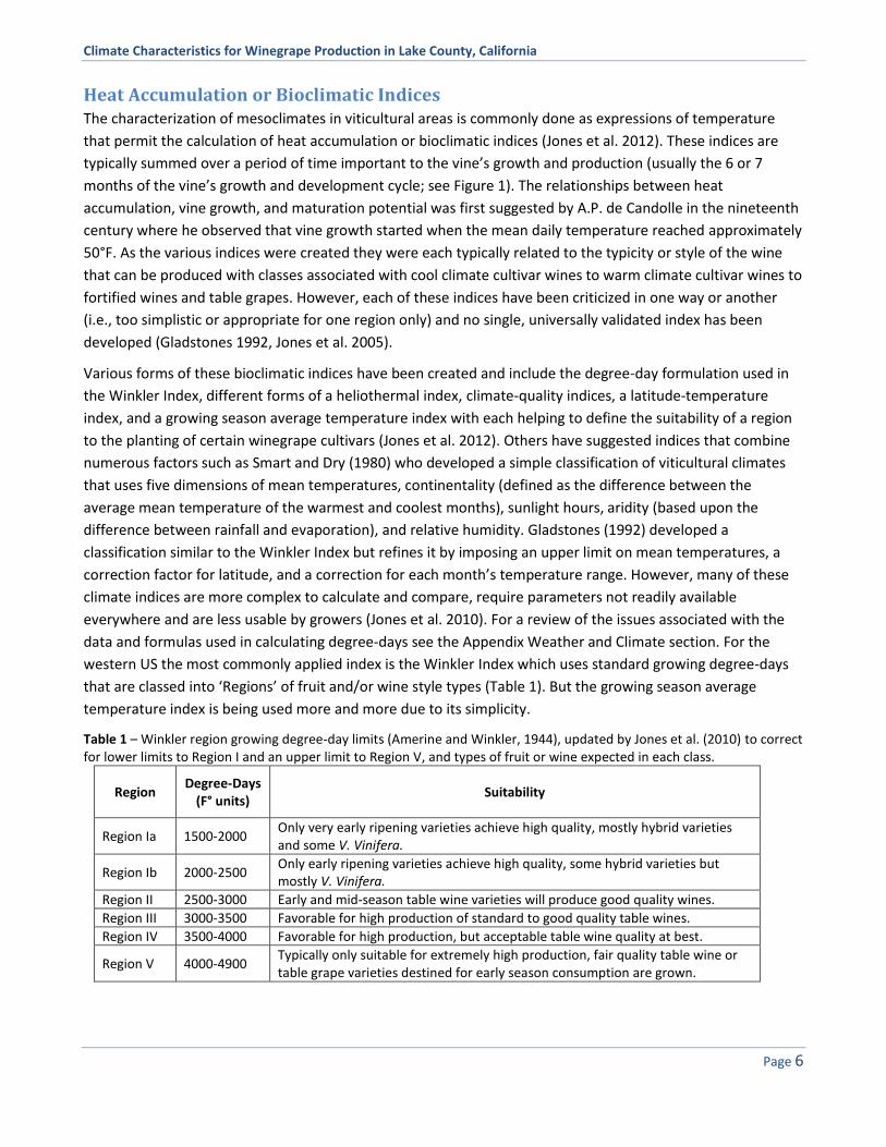
Heat Accumulation or Bioclimatic Indices The characterization of mesoclimates in viticultural areas is commonly done as expressions of temperature
that permit the calculation of heat accumulation or bioclimatic indices (Jones et al. 2012). These indices are
typically summed over a period of time important to the vine’s growth and production (usually the 6 or 7
months of the vine’s growth and development cycle; see Figure 1). The relationships between heat
accumulation, vine growth, and maturation potential was first suggested by A.P. de Candolle in the nineteenth
century where he observed that vine growth started when the mean daily temperature reached approximately
50°F. As the various indices were created they were each typically related to the typicity or style of the wine
that can be produced with classes associated with cool climate cultivar wines to warm climate cultivar wines to
fortified wines and table grapes. However, each of these indices have been criticized in one way or another
(i.e., too simplistic or appropriate for one region only) and no single, universally validated index has been
developed (Gladstones 1992, Jones et al. 2005).
Various forms of these bioclimatic indices have been created and include the degree-day formulation used in
the Winkler Index, different forms of a heliothermal index, climate-quality indices, a latitude-temperature
index, and a growing season average temperature index with each helping to define the suitability of a region
to the planting of certain winegrape cultivars (Jones et al. 2012). Others have suggested indices that combine
numerous factors such as Smart and Dry (1980) who developed a simple classification of viticultural climates
that uses five dimensions of mean temperatures, continentality (defined as the difference between the
average mean temperature of the warmest and coolest months), sunlight hours, aridity (based upon the
difference between rainfall and evaporation), and relative humidity. Gladstones (1992) developed a
classification similar to the Winkler Index but refines it by imposing an upper limit on mean temperatures, a
correction factor for latitude, and a correction for each month’s temperature range. However, many of these
climate indices are more complex to calculate and compare, require parameters not readily available
everywhere and are less usable by growers (Jones et al. 2010). For a review of the issues associated with the
data and formulas used in calculating degree-days see the Appendix Weather and Climate section. For the
western US the most commonly applied index is the Winkler Index which uses standard growing degree-days
that are classed into ‘Regions’ of fruit and/or wine style types (Table 1). But the growing season average
temperature index is being used more and more due to its simplicity.
Table 1 – Winkler region growing degree-day limits (Amerine and Winkler, 1944), updated by Jones et al. (2010) to correct for lower limits to Region I and an upper limit to Region V, and types of fruit or wine expected in each class.
Region Degree-Days
(F° units) Suitability
Region Ia 1500-2000 Only very early ripening varieties achieve high quality, mostly hybrid varieties and some V. Vinifera.
Region Ib 2000-2500 Only early ripening varieties achieve high quality, some hybrid varieties but mostly V. Vinifera.
Region II 2500-3000 Early and mid-season table wine varieties will produce good quality wines.
Region III 3000-3500 Favorable for high production of standard to good quality table wines.
Region IV 3500-4000 Favorable for high production, but acceptable table wine quality at best.
Region V 4000-4900 Typically only suitable for extremely high production, fair quality table wine or table grape varieties destined for early season consumption are grown.
Climate Characteristics for Winegrape Production in Lake County, California
Page 7
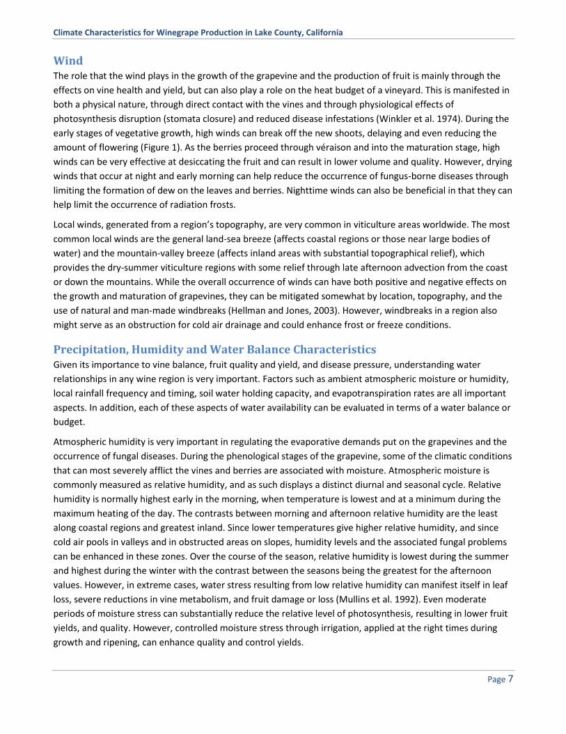
Wind The role that the wind plays in the growth of the grapevine and the production of fruit is mainly through the
effects on vine health and yield, but can also play a role on the heat budget of a vineyard. This is manifested in
both a physical nature, through direct contact with the vines and through physiological effects of
photosynthesis disruption (stomata closure) and reduced disease infestations (Winkler et al. 1974). During the
early stages of vegetative growth, high winds can break off the new shoots, delaying and even reducing the
amount of flowering (Figure 1). As the berries proceed through véraison and into the maturation stage, high
winds can be very effective at desiccating the fruit and can result in lower volume and quality. However, drying
winds that occur at night and early morning can help reduce the occurrence of fungus-borne diseases through
limiting the formation of dew on the leaves and berries. Nighttime winds can also be beneficial in that they can
help limit the occurrence of radiation frosts.
Local winds, generated from a region’s topography, are very common in viticulture areas worldwide. The most
common local winds are the general land-sea breeze (affects coastal regions or those near large bodies of
water) and the mountain-valley breeze (affects inland areas with substantial topographical relief), which
provides the dry-summer viticulture regions with some relief through late afternoon advection from the coast
or down the mountains. While the overall occurrence of winds can have both positive and negative effects on
the growth and maturation of grapevines, they can be mitigated somewhat by location, topography, and the
use of natural and man-made windbreaks (Hellman and Jones, 2003). However, windbreaks in a region also
might serve as an obstruction for cold air drainage and could enhance frost or freeze conditions.
Precipitation, Humidity and Water Balance Characteristics Given its importance to vine balance, fruit quality and yield, and disease pressure, understanding water
relationships in any wine region is very important. Factors such as ambient atmospheric moisture or humidity,
local rainfall frequency and timing, soil water holding capacity, and evapotranspiration rates are all important
aspects. In addition, each of these aspects of water availability can be evaluated in terms of a water balance or
budget.
Atmospheric humidity is very important in regulating the evaporative demands put on the grapevines and the
occurrence of fungal diseases. During the phenological stages of the grapevine, some of the climatic conditions
that can most severely afflict the vines and berries are associated with moisture. Atmospheric moisture is
commonly measured as relative humidity, and as such displays a distinct diurnal and seasonal cycle. Relative
humidity is normally highest early in the morning, when temperature is lowest and at a minimum during the
maximum heating of the day. The contrasts between morning and afternoon relative humidity are the least
along coastal regions and greatest inland. Since lower temperatures give higher relative humidity, and since
cold air pools in valleys and in obstructed areas on slopes, humidity levels and the associated fungal problems
can be enhanced in these zones. Over the course of the season, relative humidity is lowest during the summer
and highest during the winter with the contrast between the seasons being the greatest for the afternoon
values. However, in extreme cases, water stress resulting from low relative humidity can manifest itself in leaf
loss, severe reductions in vine metabolism, and fruit damage or loss (Mullins et al. 1992). Even moderate
periods of moisture stress can substantially reduce the relative level of photosynthesis, resulting in lower fruit
yields, and quality. However, controlled moisture stress through irrigation, applied at the right times during
growth and ripening, can enhance quality and control yields.

Climate Characteristics for Winegrape Production in Lake County, California
Page 8
While high levels of atmospheric moisture allow certain fungal problems to develop, the occurrence of rain
during critical growth stages can lead to devastating effects (Figure 1). While ample precipitation during the
early vegetative stage is beneficial (Jones and Davis, 2000), during bloom it can reduce or retard flowering,
during berry growth it can enhance the likelihood of fungal diseases, and during maturation it can further
fungus maladies, dilute the berries, which reduces the sugar and flavor levels, and severely limit the yield and
quality (Mullins et al. 1992). Examination of the world's viticulture regions suggests that there is no upper limit
on the amount of precipitation needed for optimum grapevine growth and production (Gladstones, 1992). On
the other hand, grapevine viability seems to be limited in some hot climates by rainfall amounts less than 20
inches, although this can be overcome by regular irrigation, if available and allowed. Extreme meteorological
events, such as thunderstorms and hail, while generally rare in most viticultural regions, are extremely
detrimental to the crop. Both events can severely damage the leaves, tendrils, and berries during growth and if
they occur during maturation can split the grapes, causing oxidation, premature fermentation, and a severe
reduction in volume and quality of the yield (Figure 1).
As an integration of many climate parameters, a soil water balance takes into account seasonal variations in
temperature, precipitation, and available soil moisture to give an estimation of water requirements (either
natural or via irrigation). A water balance essentially defines the “water need” by plants and the atmosphere in
any region. In most grape growing regions there is a period of soil water surplus from late fall through late
spring, followed by a period of draw-down of soil moisture through evaporation (by the atmosphere) and
transpiration (by plants) during the summer through the early fall, when precipitation begins replenishing the
soil. Adequate soil moisture recharge during the spring can drive vine growth and result in more effective
bloom and berry set (Williams, 2000). While some soil moisture during the summer growth period can reduce
heat stress, too high soil moisture can drive too much vegetative growth and lead to inadequate ripening
(Matthews and Anderson, 1988) along with delayed leaf fall putting the vines at risk of late fall frost/freeze
events (Figure 1).
From this summary of the importance of climate to winegrape production, the goal of this report is to help
characterize aspects of climate for winegrape production in Lake County, California (Figure 2). The following
sections provide an overview of the Lake County region, its wine industry, and the climate structure, suitability,
variability and trends.
The Lake County Region1 Lake County is found in the intermountain region of Northern California approximately 100 miles north of San
Francisco and 30-50 miles from the coast (Figure 2). The county has a total area over 1300 square miles and
ranges in elevation from approximately 600 feet where the Putah Creek crosses into Napa County in the
southeast, to the 7056 foot Snow Mountain in the wilderness area of the Mendocino National Forest along the
border with Colusa County in the northeast. The county is centered on Clear Lake, the largest natural
freshwater lake in California, with 63 square miles of surface area, and more than 100 miles of shoreline.
Lake County is part of the Southern/Central California Chaparral/Oak Woodlands US Level III ecoregion
(USEPA, 2000) that is found in an elliptical ring around the California Central Valley. It occurs on hills and
mountains ranging from 300 to 3000 ft. It is part of the Mediterranean forests, woodlands, and scrub biome of
1 For detailed information on the data used in this report see the Appendix.

Climate Characteristics for Winegrape Production in Lake County, California
Page 9
Figure 2 – Lake County American Viticultural Areas of Clear Lake, Red Hills Lake County, High Valley, Guenoc Valley, Benmore Valley, Big Valley District Lake County, and Kelsey Bench Lake County. (AVA boundaries drawn from official TTB descriptions; Code of Federal Regulations, 2013). Stars represent the weather stations used in the report (see Appendix).
California with many plant and animal species in this ecoregion adapted to periodic fire (Figure 3). The primary
distinguishing characteristic of this ecoregion is its Mediterranean-like climate of hot dry summers and cool
moist winters, and associated vegetative cover comprising mainly chaparral and oak woodlands. However,

Climate Characteristics for Winegrape Production in Lake County, California
Page 10
grasslands occur in some lower elevations and patches of pine are found at higher elevations within the
ecoregion. At the finer scale Level IV ecoregion designation, the area surrounding the lake is the Clear Lake
Hills and Valleys ecoregion (6i – Figure 4), while the remainder of Lake County shares landscape characteristics
Figure 3 – Level III ecoregions of the conterminous United States. Map Source USEPA, 2000.
Figure 4 – Level IV ecoregions in the North Coast region and Lake County (red border). Data source USEPA (2000) and
Griffith et al. (2011). The main ecoregions of Lake County and the surrounding area are described in the text.
with the Volcanic Highland ecoregion of Napa and Sonoma counties to the south (6k), the Mayacamas
Mountains ecoregion from Sonoma and Mendocino counties to the west (6j), the North Coast Range Eastern
Climate Characteristics for Winegrape Production in Lake County, California
Page 11
Slope ecoregion with Colusa and Glenn counties to the east (6g), the Foothill Ridges and Valleys with Colusa
County to the east (6f), and the High and Outer North Coast Ranges ecoregions with Glenn and Mendocino
counties to north (78q and 78r).
The Lake County Winegrape Industry Lake County has long been known as a farming community with numerous forms of agriculture serving as the
primary source of income for both early settlers and many today. Early farming consisted of cattle operations
and was followed by orchards of pears, walnuts, and plums for the prune market. Vineyards were planted in
the 1870s with varied success in numerous areas of the county and by the early 20th century the area was
earning a reputation for producing some of the world's best wines. However, similar to all other regions at the
time, Prohibition in 1920 ended Lake County's wine production. Most of the vineyards were ripped out and
replanted with walnut and pear farms. A re-emergence of the wine industry began in the 1960s when a few
growers rediscovered the area's grape growing potential and began planting vineyards.
From its early beginnings to today the wine industry in Lake County has grown to approximately 200 vineyards
representing 8253 bearing acres as of 2013 (Lake County Crop Reports). The majority of the vineyards in the
region are planted above 1,500 feet in elevation over seven TTB-approved American Viticultural Areas (AVAs)
(Figure 2). The Guenoc Valley AVA in the southern section of the county was established in 1981 (Code of
Federal Regulations, 2013; §9.26) and covers approximately 4200 acres of land at elevations that range from
nearly 1000 to 1600 ft. (Table 2). Established in 1984, the Clear Lake AVA is the largest AVA in the county at
nearly 220000 acres (Code of Federal Regulations, 2013; §9.99). The Clear Lake AVA encompasses elevations
that range from 1300 ft. to nearly 4000 ft. and is centered over the lake (Figure 2). The High Valley AVA was
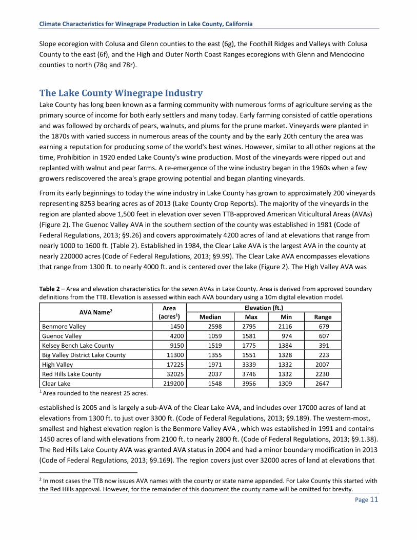
Table 2 – Area and elevation characteristics for the seven AVAs in Lake County. Area is derived from approved boundary definitions from the TTB. Elevation is assessed within each AVA boundary using a 10m digital elevation model.
AVA Name2 Area
(acres1)
Elevation (ft.)
Median Max Min Range
Benmore Valley 1450 2598 2795 2116 679
Guenoc Valley 4200 1059 1581 974 607
Kelsey Bench Lake County 9150 1519 1775 1384 391
Big Valley District Lake County 11300 1355 1551 1328 223
High Valley 17225 1971 3339 1332 2007
Red Hills Lake County 32025 2037 3746 1332 2230
Clear Lake 219200 1548 3956 1309 2647 1 Area rounded to the nearest 25 acres.
established is 2005 and is largely a sub-AVA of the Clear Lake AVA, and includes over 17000 acres of land at
elevations from 1300 ft. to just over 3300 ft. (Code of Federal Regulations, 2013; §9.189). The western-most,
smallest and highest elevation region is the Benmore Valley AVA , which was established in 1991 and contains
1450 acres of land with elevations from 2100 ft. to nearly 2800 ft. (Code of Federal Regulations, 2013; §9.1.38).
The Red Hills Lake County AVA was granted AVA status in 2004 and had a minor boundary modification in 2013
(Code of Federal Regulations, 2013; §9.169). The region covers just over 32000 acres of land at elevations that
2 In most cases the TTB now issues AVA names with the county or state name appended. For Lake County this started with the Red Hills approval. However, for the remainder of this document the county name will be omitted for brevity.
Climate Characteristics for Winegrape Production in Lake County, California
Page 12
range from close to 1300 ft. to over 3700 ft. To compare the areas and elevations of Lake County AVAs to other
California AVAs see Appendix Table 1.
The most recently approved regions are the Big Valley District Lake County and the Kelsey Bench Lake County
AVAs which were both approved in 2013 (Code of Federal Regulations, 2013; §9.232 and §9.233, respectively).
The Big Valley District represents just over 11000 acres of land at elevations from nearly 1300 ft. to 1550 ft.
while the 9150 acre Kelsey Bench is found just upslope at elevations from nearly 1400 ft. to 1775 ft. (Figure 2;
Table 2).
Of the 13646 acres planted to vines, walnuts, and pears in Lake County, vineyards make up 61% of the acreage
(Lake County Crop Reports). Growers have planted over 40 different varieties with bearing acreage reported to
represent approximately 65% red and 35% white varieties. The top seven varieties grown make up
approximately 90% of the acreage and include Cabernet Sauvignon, Sauvignon Blanc, Zinfandel, Petite Sirah,
Chardonnay, Merlot, and Syrah. In most years Cabernet Sauvignon and Sauvignon Blanc represent 50-70% of
the production, with Cabernet Sauvignon representing 30-40% of the total and Sauvignon Blanc 20-30% (Lake
County Crop Reports). Total Production has varied from 24966 to 43620 tons during 2002-2013 with overall
yields ranging from 3.5-5.3 tons per acre. Red grape production has ranged from 13658 to 25319 tons (2002-
2013) with overall yields ranging from 3.1-4.7 tons per acre. White grape production has ranged from 9620 to
18301 tons (2002-2013) with overall yields ranging from 4.3-6.3 tons per acre. While much of the fruit grown
in Lake County is produced into wine outside the region, more and more is being processed by the
approximately 35 wineries within the region.
Climate Structure At the broadest scale the weather and climate of Lake County is driven by its latitude and its location in the
westerly winds and the associated seasonality of storms coming off the Pacific. However, the strongest
regional influences are the distance from the Pacific Ocean, the moderate rain shadow effects of the coastal
mountains to the west, the landscape variations within the county, moderating winds from Clear Lake and
elevation. Combined these regional effects produce numerous microclimates within the county that vary from
other wine regions in the North Coast.
Distance to the coast and the mountains on the western edge of the county tend to limit the coastal
fog/marine influence that makes other valleys to the west cooler. The mountains also produce moderate rain
shadow effects on their leeward side, resulting in zones of lower annual rainfall across the county (see climate
section below). Furthermore the elevation of the county provides for generally higher diurnal temperature
ranges, higher UV radiation influences, and a truncation of the fall season to cool nights during ripening.
Finally, Clear Lake itself provides moderating effects due to the combination of mountain-valley breezes and
lake-land breezes. These breezes are created by temperature gradients that develop over the course of the
day over the terrain and lake, resulting in fairly consistent winds over the much of the region.
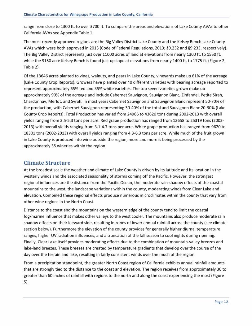
From a precipitation standpoint, the greater North Coast region of California exhibits annual rainfall amounts
that are strongly tied to the distance to the coast and elevation. The region receives from approximately 30 to
greater than 60 inches of rainfall with regions to the north and along the coast experiencing the most (Figure
5).
Climate Characteristics for Winegrape Production in Lake County, California
Page 13
Figure 5 – North Coast of California annual precipitation (1971-2000 Climate Normals). Lake County is shown with a bold red border and detailed in Figure 6. (Data Source: Daly et al. 2008).
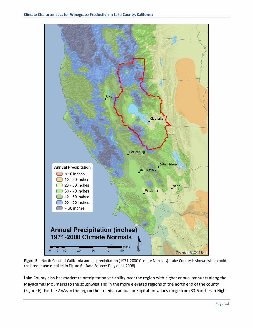
Lake County also has moderate precipitation variability over the region with higher annual amounts along the
Mayacamas Mountains to the southwest and in the more elevated regions of the north end of the county
(Figure 6). For the AVAs in the region their median annual precipitation values range from 33.6 inches in High
Climate Characteristics for Winegrape Production in Lake County, California
Page 14
Valley to 44.6 inches in Benmore Valley. However, wide ranges over the AVAs are seen with some areas in High
Valley, Kelsey Bench, Big Valley District, Clear Lake and Red Hills AVA getting less than 30 inches per year.
These drier zones are in minor rain shadow zones produced by the surrounding mountains.
Figure 6 – Lake County annual precipitation (1971-2000 Climate Normals) with the seven regional AVAs. (Data Source: Daly et al. 2008). The table on the right represents the median, maximum, and minimum values for the seven AVAs, sorted by the lowest to highest median values.
While the spatial summary of climate over Lake County above gives an overall characterization of the region, a
station summary is worth examining to better understand monthly climate parameters. For annual
precipitation the Clearlake and Lakeport stations both show the area’s dominant characteristic of a wet winter
and dry summer regime (Figure 7) averaging 31.4 inches for the 1971-2000 Climate Normals. Seasonally the
majority of the rainfall occurs during the winter with over 80% of the annual amount coming during October
through March. Most months are similar between the two stations however Lakeport shows higher November
precipitation totals while Clearlake has higher December precipitation totals.
AVA Name Median Max Min
Big Valley District 30.6 38.3 28.3
High Valley 33.6 54.1 28.3
Clear Lake 33.9 65.4 25.0
Red Hills 39.4 64.3 25.8
Kelsey Bench 35.1 41.9 29.6
Guenoc Valley 42.8 44.8 40.5
Benmore Valley 44.6 45.6 43.7

Climate Characteristics for Winegrape Production in Lake County, California
Page 15
Figure 7 – Average monthly precipitation for the Clearlake and Lakeport stations. Data for the 1971-2000 Climate
Normals. (Source: WRCC, 2013). For station locations see Figure 1.
For temperatures in the region, the best long term station is Clearlake and data from 1954-2013 provides an
examination of daily maximum and minimum averages and extremes for the location (Figure 8). Average
minimum temperatures for the Clearlake station never drop below 28°F over the year, but values between 28-
32°F occur on average between November 27th and February 11th. However, Figure 8 shows that the location
has experienced extreme minimum temperatures during the spring and fall that have dropped below 30°F into
early May and early October. Furthermore, extreme winter temperatures, dropping below 20°F have occurred
into late March and by mid-November, with the absolute minimum of 6°F occurring on December 22, 1990.
Extreme cold events such as those shown in Figure 8 are typically cold air outbreaks from Alaska or Canada and
commonly affect the entire region.
For maximum temperatures, the warmest period of the year is typically between June 22nd and September 6th,
when the daily average maximum temperatures at the Clearlake station are consistently over 90°F (Figure 8).
During the time period the location has averaged 20 days per summer over 95°F which tend to occur most
commonly between July 22nd and August 11th. Extreme maximum temperatures over 100°F have occurred as
early as May 26th and as late as October 1st, with an absolute maximum of 114°F occurring on June 30, 1977.

Climate Characteristics for Winegrape Production in Lake County, California
Page 16
Figure 8 – Clearlake station average and extreme maximum and minimum temperatures from available data during 1954-
2013 (Source: WRCC, 2013). For station location see Figure 1.
Given that Lake County has a seasonally dry climate, understanding overall water needs for irrigation is
important for sustainable growth and production. Plant water requirements are typically described by the
evapotranspiration rate (ET). ET is the combined amount of evaporation and plant transpiration from the
Earth's land surface to the atmosphere. Factors that affect ET include a given plant's growth stage, the type of
soil, the percentage of soil ground cover, solar radiation, humidity, temperature, and wind. Five year averages
for Kelseyville, Red Hills, and Guenoc Valley show that the locations experience average daily ET rates that
mirror the temperature regime for the region (Figure 9). Averaged over the three locations reference ETo rates
climb above 0.10 inches per day by March 10th and 0.20 inches per day by May 6th and drop below these values
on September 5th (0.20 inches per day) and October 4th (0.10 inches per day) (Figure 9). Onset of these ETo
levels is similar across the three stations although peak ETo during the middle of the summer is slightly higher
in Guenoc Valley. Total growing season (April-October) ETo values average 39.9 inches for the three locations,
ranging from 38.4 inches for Kelseyville, to 39.5 inches for Red Hills, and to 41.9 inches for Guenoc Valley.
From these observations, the theoretical total amount of ET ‘need’ by the climate is roughly 40 inches during
the growing season. However, the ETo is the ‘reference ET’ for the location, meaning that the value needs to
be adjusted to the crop. The adjustment to crop ET is done by a coefficient, which typically changes over the
growing season to account for the growth stage and size of the crop’s canopy. For winegrapes the method
would have the crop coefficient start out at approximately 20% of reference ETo in the spring, increasing to
50% of reference ETo by mid-canopy growth, and then plateauing at 65% of reference ETo until the end of the
Climate Characteristics for Winegrape Production in Lake County, California
Page 17
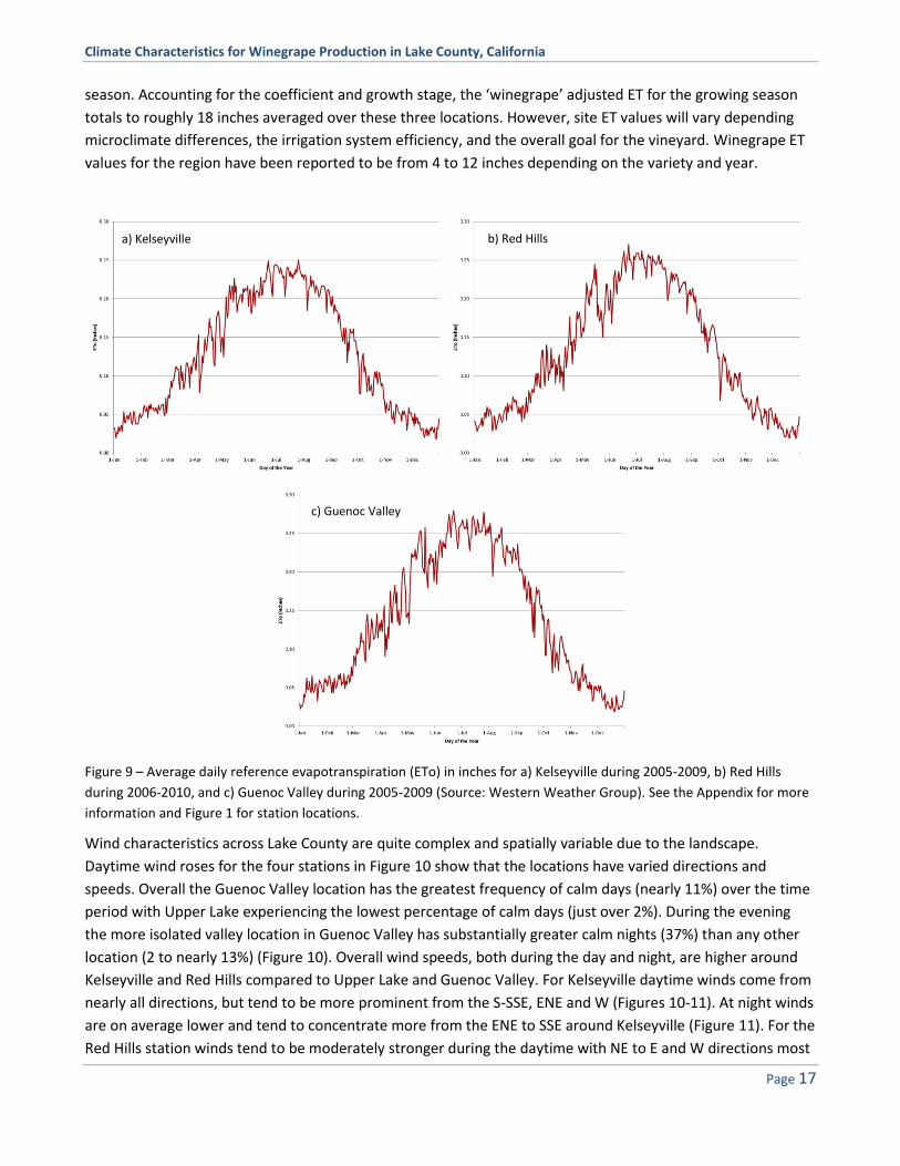
season. Accounting for the coefficient and growth stage, the ‘winegrape’ adjusted ET for the growing season
totals to roughly 18 inches averaged over these three locations. However, site ET values will vary depending
microclimate differences, the irrigation system efficiency, and the overall goal for the vineyard. Winegrape ET
values for the region have been reported to be from 4 to 12 inches depending on the variety and year.
Figure 9 – Average daily reference evapotranspiration (ETo) in inches for a) Kelseyville during 2005-2009, b) Red Hills
during 2006-2010, and c) Guenoc Valley during 2005-2009 (Source: Western Weather Group). See the Appendix for more
information and Figure 1 for station locations.
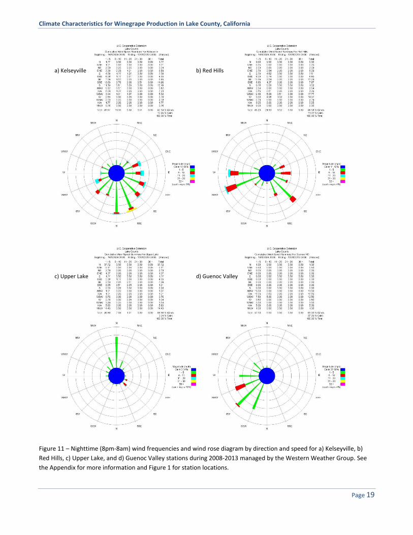
Wind characteristics across Lake County are quite complex and spatially variable due to the landscape.
Daytime wind roses for the four stations in Figure 10 show that the locations have varied directions and
speeds. Overall the Guenoc Valley location has the greatest frequency of calm days (nearly 11%) over the time
period with Upper Lake experiencing the lowest percentage of calm days (just over 2%). During the evening
the more isolated valley location in Guenoc Valley has substantially greater calm nights (37%) than any other
location (2 to nearly 13%) (Figure 10). Overall wind speeds, both during the day and night, are higher around
Kelseyville and Red Hills compared to Upper Lake and Guenoc Valley. For Kelseyville daytime winds come from
nearly all directions, but tend to be more prominent from the S-SSE, ENE and W (Figures 10-11). At night winds
are on average lower and tend to concentrate more from the ENE to SSE around Kelseyville (Figure 11). For the
Red Hills station winds tend to be moderately stronger during the daytime with NE to E and W directions most
a) Kelseyville b) Red Hills
c) Guenoc Valley

Climate Characteristics for Winegrape Production in Lake County, California
Page 18
Figure 10 – Daytime (8am-8pm) wind frequencies and wind rose diagram by direction and speed for a) Kelseyville, b) Red
Hills, c) Upper Lake, and d) Guenoc Valley stations during 2008-2013 managed by the Western Weather Group. See the
Appendix for more information and Figure 1 for station locations.
a) Kelseyville b) Red Hills
d) Guenoc Valley c) Upper Lake
Climate Characteristics for Winegrape Production in Lake County, California
Page 19
Figure 11 – Nighttime (8pm-8am) wind frequencies and wind rose diagram by direction and speed for a) Kelseyville, b)
Red Hills, c) Upper Lake, and d) Guenoc Valley stations during 2008-2013 managed by the Western Weather Group. See
the Appendix for more information and Figure 1 for station locations.
a) Kelseyville b) Red Hills
d) Guenoc Valley c) Upper Lake
Climate Characteristics for Winegrape Production in Lake County, California
Page 20
common, while at night winds tend to be more commonly from the W-WSW and SE. For Upper Lake winds are
typically lower in speed and tend to come mostly from the S-SE or N directions during the daytime. These
relatively low wind speeds are either off the surrounding mountains from the north or off the lake from the
south. Higher daytime winds at Upper Lake are more frequent from the SE (Figure 10). Nighttime winds at
Upper Lake are very low and predominately from the north where cool nighttime air moves southward. For
Guenoc Valley daytime winds come from nearly all directions, but tend to come from the E-ESE most often
(Figure 10). When nighttime winds do occur at the Guenoc Valley location, they are most commonly from
WSW to SSW (Figure 11).
For growing degree-days (GDD), the North Coast region provides a wide range of climates for viticulture. GDD
values below 1500 are typically found right along the coast and in the mountains in the north (Figure 12). On
the other end of the spectrum Region V GDD values (4000-4900) can be seen starting in the western foothills
of the Central Valley. Numerous areas of Region Ia and Ib can be found near the coast and at elevation (Figure
12) while areas with Region III and IV occur in the intermountain valleys throughout the North Coast. To
compare the growing degree-day characteristics of Lake County AVAs to other California AVAs see Appendix
Table 1.

Climate Characteristics for Winegrape Production in Lake County, California
Page 21
Figure 12 – North Coast of California average growing degree-days (F° units, Apr-Oct, base 50°F and no upper limit; 1971-2000 Climate Normals). Note that the class ranges mapped here corresponds to traditional Winkler Regions (Winkler et al. 1974) and updates to the lower Region I class and limits to the Region V class found by Jones et al. (2010) and Hall and Jones (2010). Lake County is shown with a bold red border and detailed in Figure 13. (Data Source: Daly et al. 2008). To examine the growing degree-day spatial characteristics of North Coast and other California AVAs see Appendix Table 1.

Climate Characteristics for Winegrape Production in Lake County, California
Page 22
The magnitude of the effect of both distance from the coast and elevation on both the overall amount and
seasonal structure of growing degree-day values can be seen in a transect of locations going from the coast to
the Sierra Nevadas (Figure 13). Accumulation of GDD starts and ends when the average daily temperatures are
above 50°F and Figure 13 shows the effect of location with more inland and higher elevation locations having
lower values accumulated over a shorter period. A coastal location such as Fort Bragg has a longer
accumulation period than higher elevation and inland locations, but low total amount due to lower year round
temperatures. Two locations in close proximity – Ukiah and Clear Lake – have similar peak GDD, but Ukiah
accumulates more over a broader window of time due to its lower elevation and closer proximity to the coast.
Conversely the growing season ends sooner in Clear Lake with cooler nighttime temperatures during ripening.
Figure 13 – Monthly average growing degree-days (F° units, base 50°F and no upper limit; 1971-2000 Climate Normals) for a transect of climate stations from the coast to the mountains. Legend includes the elevation of the station and the total growing season (Apr-Oct) growing degree-days. (Data Source: WRCC, 2013).
Growing degree-days over Lake County varies mostly due to elevation, but also generally increases as you head
inland (Figure 14). The county as a whole averages 3215 GDD (1971-2000 climate normals) with a standard
deviation of 398 GDD, while the seven AVAs average 3274 (Table in Figure 14). The lowest values are found in
the northern portion of the county with values below 1500 GDD in the higher elevations around Snow
Mountain. The highest GDD in the county is observed along the eastern border with Colusa County where
values over 4300 GDD are experienced. By AVA, the Big Valley District has the lowest median of the seven
regions, but is very similar to Benmore Valley, Kelsey Bench, and Clear Lake. The Red Hills AVA has the highest
median GDD and the lowest range between the coolest and warmest sites within the AVA (Figure 14).
Short-term records from the station network managed by Western Weather Group for the Lake County
Winegrape Commission confirm these values. Three stations on a transect from the southern end of the Kelsey
Bench AVA to the northern end of the Big Valley District AVA show values averaging nearly 3100 GDD from

Climate Characteristics for Winegrape Production in Lake County, California
Page 23
2005 through 2010. In addition, three stations in the Red Hill AVA average nearly 3600 GDD over the same
time period.
GDD values such as those summarized for the Lake County AVAs in Figure 14 range from a high Region II in the
coolest zones (2799 GDD) to high Region IV (3811 GDD) in the warmest zones of the Clear Lake AVA. For the
AVA median GDD values the area would be classed as mostly a Region III or very low Region IV.
Figure 14 – Lake County average growing degree-days (F° units, Apr-Oct, base 50°F and no upper limit; 1971-2000 Climate Normals) with the seven regional AVAs. Note that the class ranges mapped here corresponds to traditional Winkler Regions (Winkler et al. 1974) and updates to the lower Region I class and limits to the Region V class found by Jones et al. (2010) and Hall and Jones (2010). (Data Source: Daly et al. 2008). The table on the right represents the median, maximum, and minimum values for the seven AVAs, sorted by the lowest to highest median values.
Median dates of the last spring frost (32°F) over the North Coast occur before March 1st in Marin County, the
southern portions of Napa and Sonoma counties, surrounding Santa Rosa and Healdsburg and along the coast
(Figure 15). Later last spring frosts can be found inland and with higher elevations in portions of northern Lake
County and Mendocino County.
AVA Name Median Max Min
Big Valley District 3245 3281 3171
Benmore Valley 3248 3332 3155
Kelsey Bench 3250 3593 3189
Clear Lake 3267 3811 2799
Guenoc Valley 3481 3796 3420
High Valley 3548 3755 3139
Red Hills 3595 3753 3155
To compare the growing degree-day
characteristics of Lake County AVAs to other
California AVAs see Appendix Table 1.

Climate Characteristics for Winegrape Production in Lake County, California
Page 24
Figure 15 – North Coast of California median date of the last spring frost (32°F; 1971-2000 Climate Normals). Lake County is shown with a bold red border and detailed in Figure 16. (Data Source: Daly et al. 2008).
Within Lake County last spring frosts range from the second two weeks in March for areas in and around Red
Hills AVA, High Valley AVA, and Guenoc Valley AVA to frosts occurring after April 30th across higher elevations
and most of the northern portion of the county (Figure 16). By AVA, Kelsey Bench and the Big Valley District

Climate Characteristics for Winegrape Production in Lake County, California
Page 25
have the latest average last spring frosts of April 18th due to relatively gradual slopes and pooling of cooler air
from the surrounding hillsides. The Guenoc, Benmore, and High valleys have average last spring frosts in the
early part of April due to areas where cool air pooling is more limited and inversions more common.
Figure 16 – Lake County median date of the last spring frost (32°F; 1971-2000 Climate Normals) with the seven regional AVAs. (Data Source: Daly et al. 2008). The table on the right represents the median, maximum, and minimum values for the seven AVAs, sorted by the latest to earliest median values.
First fall frosts show a prominent valley-first pattern indicating that the onset of frost during the fall is likely
driven by pooling of cooler air influenced by lower wind speeds (Figure 17). The earliest median first fall frosts
are seen in late September and early October in the valleys in northern Mendocino County and surrounding
Clear Lake and the latest in late November or early December along the coast or with elevation in many areas.
AVA Name Median Max Min
Kelsey Bench 18-Apr 21-Apr 5-Apr
Big Valley District 18-Apr 20-Apr 4-Apr
Clear Lake 16-Apr 1-May 22-Mar
Guenoc Valley 7-Apr 10-Apr 18-Mar
Benmore Valley 3-Apr 7-Apr 2-Apr
High Valley 2-Apr 23-Apr 23-Mar
Red Hills 31-Mar 16-Apr 22-Mar

Climate Characteristics for Winegrape Production in Lake County, California
Page 26
Figure 17 – North Coast of California median date of the first fall frost (32°F; 1971-2000 Climate Normals). Lake County is shown with a bold red border and detailed in Figure 18. (Data Source: Daly et al. 2008).
For Lake County the earliest fall frosts show a similar pattern around Clear Lake as compared to the last spring
frost (Figure 18). However, the first fall frost shows a more prominent valley pattern in the north of the county
compared to the widespread areas with similar last spring frosts (Figure 15). Across the broad flatter zones

Climate Characteristics for Winegrape Production in Lake County, California
Page 27
around the Big Valley District AVA, Kelsey Bench AVA, and surrounding Clear Lake the earliest first fall frosts
occur in the last few days of October and the first week in November on average. Guenoc Valley AVA also has a
slightly earlier onset of fall frosts due to its valley location, while Benmore Valley does not appear to have first
fall frost onset until the first to second week in December.
Figure 18 – Lake County median date of the first fall frost (32°F; 1971-2000 Climate Normals) with the seven regional AVAs. (Data Source: Daly et al. 2008). The table on the right represents the median, maximum, and minimum values for the seven AVAs, sorted by the earliest to latest median values.
The frost-free season reflects the difference between the last spring and first fall frosts and mapped over the
North Coast shows that the majority of the wine regions have greater than 180 day periods (Figure 19). The
shortest periods are found in the mountainous region to the north and within some of the intermountain
valleys across the region. The longest periods are found in the Central Valley, in Marin County, the southern
end of Napa County, throughout much of Sonoma County, and along the coast.
AVA Name Median Max Min
Big Valley District 30-Oct 18-Nov 27-Oct
Kelsey Bench 2-Nov 18-Nov 29-Oct
Clear Lake 3-Nov 7-Dec 22-Oct
Guenoc Valley 10-Nov 4-Dec 6-Nov
High Valley 25-Nov 4-Dec 28-Oct
Red Hills 27-Nov 3-Dec 26-Oct
Benmore Valley 8-Dec 8-Dec 6-Dec

Climate Characteristics for Winegrape Production in Lake County, California
Page 28
Figure 19 – North Coast of California median length of the frost-free period (between the median last spring and first fall dates with 32°F; 1971-2000 Climate Normals) with the seven regional AVAs. Lake County is shown with a bold red border and detailed in Figure 20. (Data Source: Daly et al. 2008).
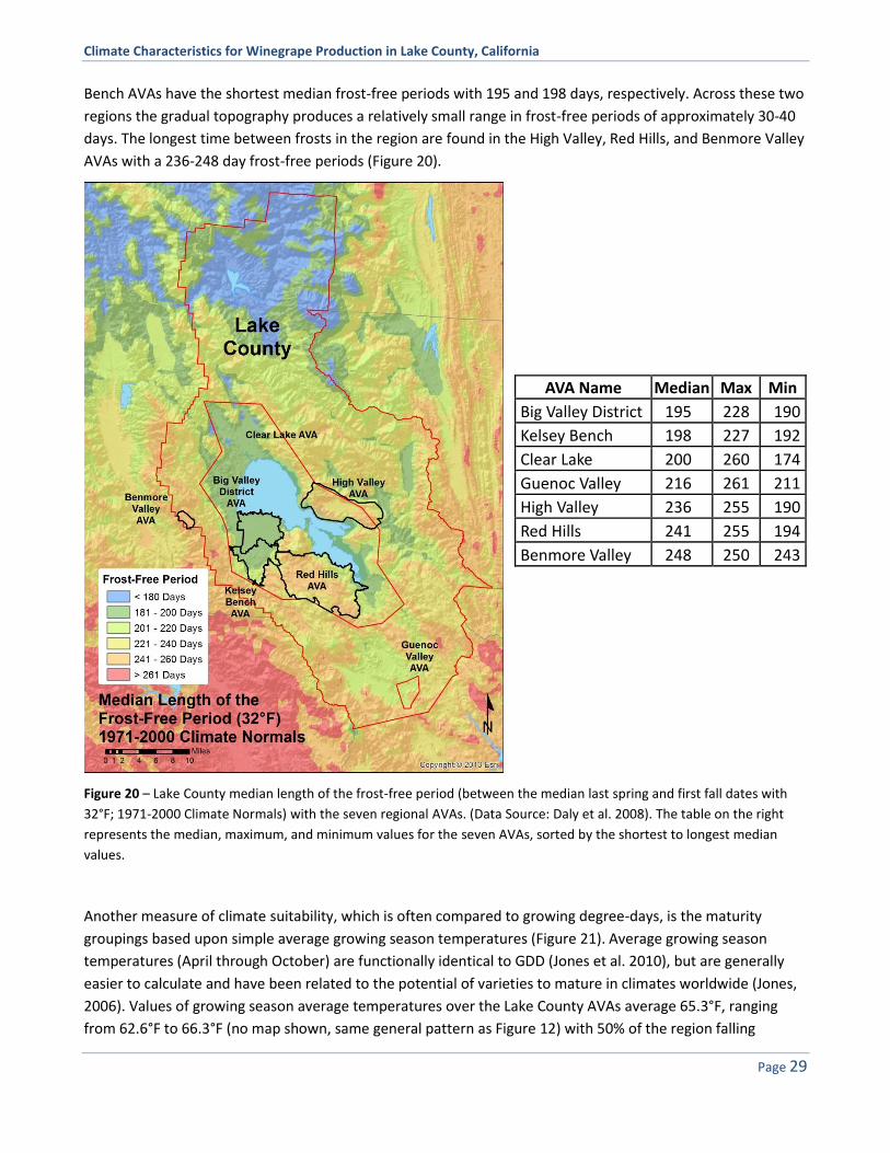
Within Lake County the frost-free period varies from less than 180 days over much of the northern portion of
the county to many zones with 240 days or longer between frosts (Figure 20). The Big Valley District and Kelsey
Climate Characteristics for Winegrape Production in Lake County, California
Page 29
Bench AVAs have the shortest median frost-free periods with 195 and 198 days, respectively. Across these two
regions the gradual topography produces a relatively small range in frost-free periods of approximately 30-40
days. The longest time between frosts in the region are found in the High Valley, Red Hills, and Benmore Valley
AVAs with a 236-248 day frost-free periods (Figure 20).
Figure 20 – Lake County median length of the frost-free period (between the median last spring and first fall dates with
32°F; 1971-2000 Climate Normals) with the seven regional AVAs. (Data Source: Daly et al. 2008). The table on the right
represents the median, maximum, and minimum values for the seven AVAs, sorted by the shortest to longest median
values.
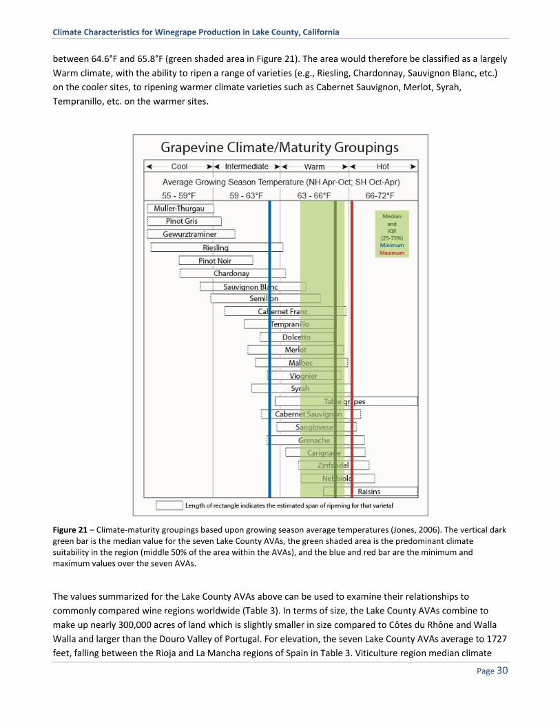
Another measure of climate suitability, which is often compared to growing degree-days, is the maturity
groupings based upon simple average growing season temperatures (Figure 21). Average growing season
temperatures (April through October) are functionally identical to GDD (Jones et al. 2010), but are generally
easier to calculate and have been related to the potential of varieties to mature in climates worldwide (Jones,
2006). Values of growing season average temperatures over the Lake County AVAs average 65.3°F, ranging
from 62.6°F to 66.3°F (no map shown, same general pattern as Figure 12) with 50% of the region falling
AVA Name Median Max Min
Big Valley District 195 228 190
Kelsey Bench 198 227 192
Clear Lake 200 260 174
Guenoc Valley 216 261 211
High Valley 236 255 190
Red Hills 241 255 194
Benmore Valley 248 250 243
Climate Characteristics for Winegrape Production in Lake County, California
Page 30
between 64.6°F and 65.8°F (green shaded area in Figure 21). The area would therefore be classified as a largely
Warm climate, with the ability to ripen a range of varieties (e.g., Riesling, Chardonnay, Sauvignon Blanc, etc.)
on the cooler sites, to ripening warmer climate varieties such as Cabernet Sauvignon, Merlot, Syrah,
Tempranillo, etc. on the warmer sites.
Figure 21 – Climate-maturity groupings based upon growing season average temperatures (Jones, 2006). The vertical dark green bar is the median value for the seven Lake County AVAs, the green shaded area is the predominant climate suitability in the region (middle 50% of the area within the AVAs), and the blue and red bar are the minimum and maximum values over the seven AVAs.
The values summarized for the Lake County AVAs above can be used to examine their relationships to
commonly compared wine regions worldwide (Table 3). In terms of size, the Lake County AVAs combine to
make up nearly 300,000 acres of land which is slightly smaller in size compared to Côtes du Rhône and Walla
Walla and larger than the Douro Valley of Portugal. For elevation, the seven Lake County AVAs average to 1727
feet, falling between the Rioja and La Mancha regions of Spain in Table 3. Viticulture region median climate

Climate Characteristics for Winegrape Production in Lake County, California
Page 31
values (both GST and GDD) place the Lake County AVAs as one of the warmer of the regions examined, falling
in between the Alexander Valley AVA and the Napa Valley AVA. Comparable areas outside the US include the
Douro Valley of Portugal and the Chianti region of Italy, both of which are on average slightly cooler than the
Lake County AVAs. Compared to other AVAs in the western US, the Lake County AVAs are moderately warm,
ranking 81st (Benmore Valley AVA) to 105th (Red Hills AVA) out of 135 AVAs in median GDD with similar regions
being the Oak Knoll District, Chiles Valley, Fiddletown, and Shenandoah Valley AVAs (Jones et al. 2010).
Table 3 – Wine producing region total area and spatial median values for elevation and climate indices for Europe over 1950-2000 (Jones et al. 2009), Australia for 1971-2000 (Hall and Jones 2010), New Zealand wine regions for 1971-2000 (Anderson et al. 2012), and the western United States for 1971-2000 (Jones et al. 2010). Values for Lake County are the total area of all seven AVAs and the median elevation and climate index values across all seven AVAs. Climate indices are growing season average temperature (GST, °F) and growing degree-days (GDD, F° units). The table is sorted by GST.
Country/State Region Area (acres) Elevation (ft.) GST (°F) GDD
Germany Mosel Valley 48927 587 57.9 1804 Germany Rhine Valley 80803 558 58.1 1860 France Champagne 94147 558 58.2 1865 Germany Baden 46703 804 58.8 1901 Oregon Willamette Valley 3428829 400 59.0 1922 New Zealand Wairau Valley (Marlborough) 150981 262 59.2 1946 France Burgundy 64247 866 59.4 2012 Italy Valtellina Superiore 1236 1561 61.2 2403 New Zealand Hawkes Bay 148016 95 61.3 2401 France Bordeaux 363491 164 61.7 2497 Spain Rioja 149499 1660 61.9 2538 Australia Yarra Valley 770968 823 61.9 2417 Washington & Oregon Walla Walla 322719 1040 62.8 2750 France Côtes du Rhône Méridionales 355831 571 63.1 2826 Australia Coonawarra 98842 213 63.3 2720 Italy Barolo 13838 1030 63.5 2880 Italy Vino Nobile di Montepulciano 6919 1007 63.5 2903 Portugal Vinho Verde 15073 623 63.7 2943 Italy Chianti Classico 24958 1053 64.2 3033 Portugal Douro Valley 199414 1433 64.2 3031 California Alexander Valley 78322 485 64.6 3134 California Lake County AVAs 294550 1727 65.3 3274 California Napa Valley 401299 813 65.8 3389 California Paso Robles 608867 1305 66.0 3425 Spain La Mancha 707709 2260 66.0 3442 Australia Barossa Valley 145792 912 66.2 3334 Australia Margaret River 652357 246 66.6 3397 California Lodi 542395 78.7 68.5 3980 Spain Jerez-Xéres-Sherry 31135 187 69.6 4217
Climate Variability While the average climate structure in a region determines the broad suitability of winegrape cultivars, climate
variability influences issues of production and quality risk associated with how equitable the climate is year in
year out. Climate variability in wine regions influences grape and wine production through cold temperature

Climate Characteristics for Winegrape Production in Lake County, California
Page 32
extremes during the winter in some regions, frost frequency and severity during the spring and fall, high
temperature events during the summer, extreme rain or hail events, and broad spatial and temporal drought
conditions. Climate variability mechanisms that influence wine regions are tied to large scale atmospheric and
oceanic interactions that operate at different spatial and temporal scales. The most prominent of these is the
large scale tropical Pacific sector El Niño-Southern Oscillation (ENSO; Figure 22), which has broad influences on
wine region climates in North America, Australia and New Zealand, South Africa, South America, and Europe
(Jones et al. 2012). However, the effects of ENSO on wine region climate variability differs tremendously in
magnitude and has opposite effects depending on the location of the wine region and is often coupled with
other more influential regional mechanisms (Jones and Goodrich, 2008).
Figure 22 – Main phases of the El Niño Southern Oscillation (ENSO), El Niño or warm phase (left) and La Niña or cool phase (right). ). Note that there is a neutral phase as well, it occurs when the SSTs in the Tropical Pacific are near normal. (Image Source: http://www.climate.gov/)
Variability in the climate of the western US wine regions is largely influenced by conditions in the North Pacific
and Tropical Pacific oceans which in turn affect the circulation of the atmosphere (Mantua and Hare, 2002;
Jones and Goodrich, 2008). The two main mechanisms in the Pacific are sea surface temperatures (SSTs) that
drive variations in the Pacific Decadal Oscillation (PDO, North Pacific) and El Niño/La Niña (ENSO, Tropical
Pacific). The main difference between the two, besides location, is that the PDO is long term (multi-decadal
swings) and ENSO is short term (2-5 year swings). Both ENSO and PDO represent measures of variation in the
ocean and atmosphere and are tabulated as an index for comparing conditions during seasons or years.
For temperature, El Niño winters (November to March) tend to be warmer than normal in the PNW while
California is normal to slightly cooler than normal (Figure 23). On the other hand La Niña winters are

Climate Characteristics for Winegrape Production in Lake County, California
Page 33
Figure 23 – Temperature anomalies observed during El Niño (left) and La Niña (right) events for winter (top: November-March) and summer (bottom: May-September) from 1948-2010. Anomalies are based upon the 1971-2000 Climate Normals and boundaries shown are the US climate divisions. Map Source: NOAA/ESRL Physical Sciences Division.
generally cooler than average over the western US. During the summer El Niño effects tend to be minimal over
much of the west, while La Niña years can have lingering cooler than normal conditions into the summer (like
the 2010 and 2011 vintages) and over most of the region (Figure 23). In terms of the risk of extreme warm or
cold years, winter temperatures are 1.5 to 2.0 times more likely to be warmer during El Niño events, while
winter temperature extremes are near normal to 2.0 times more likely to be colder during La Niña events
(Figure 24). For the spring, temperatures are 2.0 times more likely to be warmer during El Niño events but near
normal during La Niña years. During the summer the risk of extreme years is low in the North Coast during El
Niño events and 1.5 times more likely to be warmer during La Niña events. Risk of extreme fall conditions is
minimal during La Niña events but 1.5 times more likely to be cold during El Niño events (Figure 24).
El Niño Winter
El Niño Summer
La Niña Winter
La Niña Summer

Climate Characteristics for Winegrape Production in Lake County, California
Page 34
For precipitation, El Niño winters are much wetter in California and dry into northern Oregon and Washington while La Niña winters are wetter from northern California to the Canadian border and southern California is drier (Figure 25). Summer precipitation variability is not affected much by either El Niño or La Niña conditions. In terms of the risk of wet or dry years, winters in the North Coast are 2.0 times more likely to be wetter than normal during El Niño events and normal during La Niña events. Spring experiences similar risk compared to winter with wet years 1.75 times more likely with El Niño and normal with La Niña (Figure 26). During the
El Niño La Niña
El Niño La Niña
El Niño La Niña
El Niño La Niña
El Niño
Figure 24 – Winter (Dec-Jan-Feb; top row), spring (Mar-Apr-May; 2nd row), summer (Jun-Jul-Aug; 3rd row), and fall (Sep-Oct-Nov; bottom row) risk of temperature extremes with ENSO conditions preceding the season. Results are based on the US climate division dataset for 1896-1995. Extreme is defined as being in the highest or lowest 20% of the 100 year record. ENSO is defined as the top 20 El Niño years (left panel) and top 20 La Niña years (right panel). Map Source: NOAA/ESRL Physical Sciences Division.

Climate Characteristics for Winegrape Production in Lake County, California
Page 35
summer, La Niña events are 1.75 times more likely to produce dry conditions while El Niño events are normal. For the North Coast, the risk of dry or wet falls is normal for both ENSO conditions.
Figure 25 – Precipitation anomalies observed during El Niño (left) and La Niña (right) events for winter (top: November-March) and summer (bottom: May-September) from 1948-2010. Anomalies are based upon the 1971-2000 Climate Normals and boundaries shown are the US climate divisions. Map Source: NOAA/ESRL Physical Sciences Division.
El Niño Winter
El Niño Summer
La Niña Winter
La Niña Summer

Climate Characteristics for Winegrape Production in Lake County, California
Page 36
As the dominant long term climate variability mechanism for western North American, the Pacific Decadal
Oscillation (PDO; Figure 27) is a result of low-frequency variability in sea surface temperatures (SSTs) in the
North Pacific Ocean (Frauenfeld et al. 2005). Like ENSO, the PDO is an index representing the main variability
structure in mean monthly SSTs in the Pacific Ocean north of 20°N latitude (Mantua and Hare, 2002) and is
related to the circulation of the atmosphere across the mid-latitudes. Positive (warm phase) values of the PDO
refer to above normal SSTs along the west coast of North America and below normal SSTs in the central and
El Niño La Niña
El Niño La Niña
El Niño La Niña
El Niño La Niña
Figure 26 – Winter (Dec-Jan-Feb; top row), spring (Mar-Apr-May; 2nd row), summer (Jun-Jul-Aug; 3rd row), and fall (Sep-Oct-Nov; bottom row) risk of precipitation extremes with ENSO conditions preceding the season. Results are based on the US climate division dataset for 1896-1995. Extreme is defined as being in the highest or lowest 20% of the 100 year record. ENSO is defined as the top 20 El Niño years (left panel) and top 20 La Niña years (right panel). Map Source: NOAA/ESRL Physical Sciences Division.
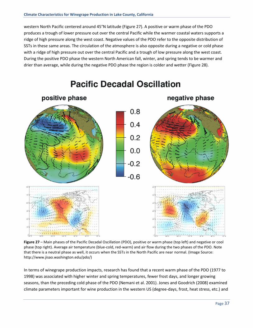
Climate Characteristics for Winegrape Production in Lake County, California
Page 37
western North Pacific centered around 45°N latitude (Figure 27). A positive or warm phase of the PDO
produces a trough of lower pressure out over the central Pacific while the warmer coastal waters supports a
ridge of high pressure along the west coast. Negative values of the PDO refer to the opposite distribution of
SSTs in these same areas. The circulation of the atmosphere is also opposite during a negative or cold phase
with a ridge of high pressure out over the central Pacific and a trough of low pressure along the west coast.
During the positive PDO phase the western North American fall, winter, and spring tends to be warmer and
drier than average, while during the negative PDO phase the region is colder and wetter (Figure 28).
Figure 27 – Main phases of the Pacific Decadal Oscillation (PDO), positive or warm phase (top left) and negative or cool phase (top right). Average air temperature (blue-cold, red-warm) and air flow during the two phases of the PDO. Note that there is a neutral phase as well, it occurs when the SSTs in the North Pacific are near normal. (Image Source: http://www.jisao.washington.edu/pdo/)
In terms of winegrape production impacts, research has found that a recent warm phase of the PDO (1977 to
1998) was associated with higher winter and spring temperatures, fewer frost days, and longer growing
seasons, than the preceding cold phase of the PDO (Nemani et al. 2001). Jones and Goodrich (2008) examined
climate parameters important for wine production in the western US (degree-days, frost, heat stress, etc.) and
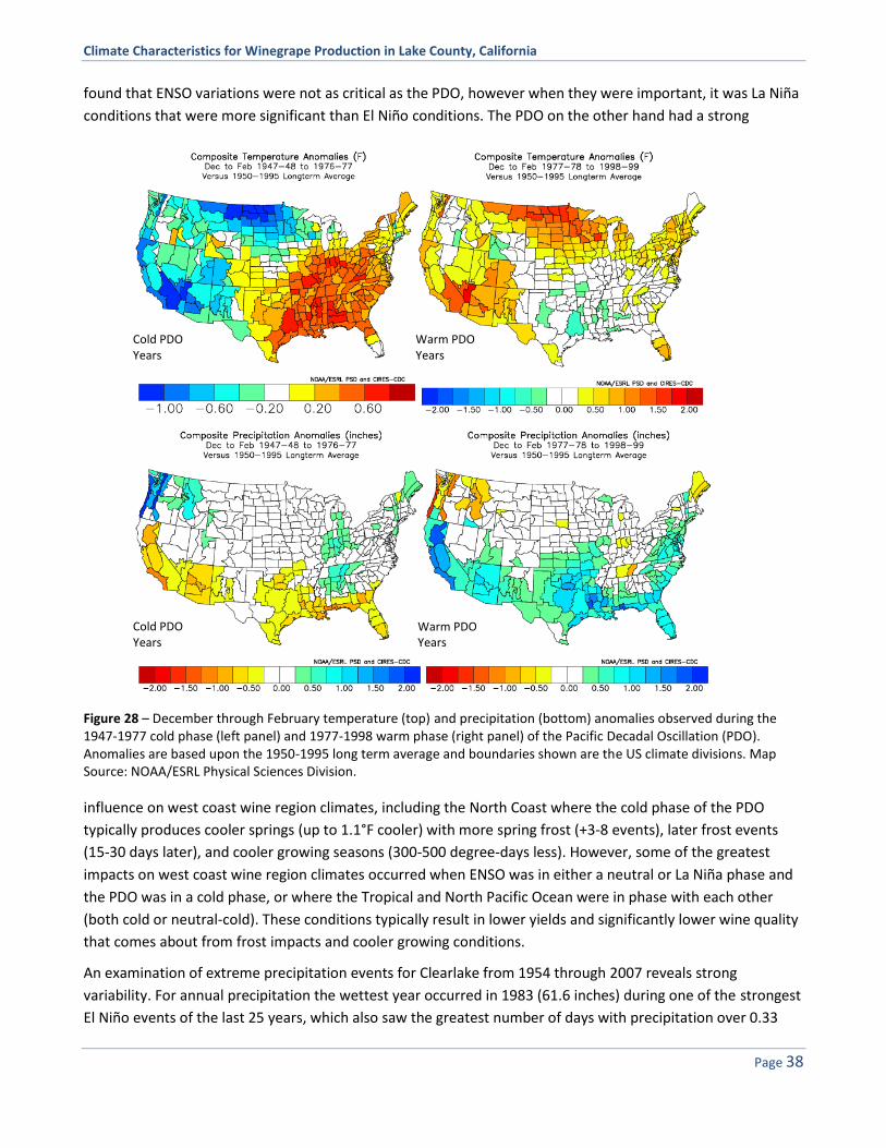
Climate Characteristics for Winegrape Production in Lake County, California
Page 38
found that ENSO variations were not as critical as the PDO, however when they were important, it was La Niña
conditions that were more significant than El Niño conditions. The PDO on the other hand had a strong
Figure 28 – December through February temperature (top) and precipitation (bottom) anomalies observed during the 1947-1977 cold phase (left panel) and 1977-1998 warm phase (right panel) of the Pacific Decadal Oscillation (PDO). Anomalies are based upon the 1950-1995 long term average and boundaries shown are the US climate divisions. Map Source: NOAA/ESRL Physical Sciences Division.
influence on west coast wine region climates, including the North Coast where the cold phase of the PDO
typically produces cooler springs (up to 1.1°F cooler) with more spring frost (+3-8 events), later frost events
(15-30 days later), and cooler growing seasons (300-500 degree-days less). However, some of the greatest
impacts on west coast wine region climates occurred when ENSO was in either a neutral or La Niña phase and
the PDO was in a cold phase, or where the Tropical and North Pacific Ocean were in phase with each other
(both cold or neutral-cold). These conditions typically result in lower yields and significantly lower wine quality
that comes about from frost impacts and cooler growing conditions.
An examination of extreme precipitation events for Clearlake from 1954 through 2007 reveals strong
variability. For annual precipitation the wettest year occurred in 1983 (61.6 inches) during one of the strongest
El Niño events of the last 25 years, which also saw the greatest number of days with precipitation over 0.33
Cold PDO Years
Warm PDO Years
Cold PDO Years
Warm PDO Years

Climate Characteristics for Winegrape Production in Lake County, California
Page 39
inches (47 days) or 1.0 inch (19 days). Conversely the driest year occurred in 1976 (7.9 inches) which occurred
at the onset of the last cold PDO period, while the longest period of consecutive dry days was 169 days in 2002
during a combined La Niña-cold PDO year. Table 4 shows the complexities of these relationships for growing
season (April through October) climate characteristics for the Clearlake station during 1954-2007. Cool growing
Table 4 – The Clearlake station’s general growing season climate characteristics within ENSO/PDO phases from 1954-2007. ENSO-PDO phases as detailed in Jones and Goodrich (2008). Note that not all differences here are statistically significant.
Years with ENSO/PDO
State
Average Temperature
(°F)
Maximum Temperature
(°F)
Minimum Temperature
(°F)
Growing Degree-Days (F°
units)
Precipitation (inches)
# of Days Temperature
> 95°F
# of Days Temperature
< 32°F
Warm PDO - El Niño 1977, 1980 1983, 1987 1988, 1992 1995, 1998 2003, 2004 2005
64.7 81.4 48.1 3315 5.2 27 2
Cold PDO - El Niño 1958, 1964 1966, 1969 1970, 1973 2007
65.1 84.3 46.0 3290 2.8 45 11
Warm PDO - La Niña 1985, 1986 1989
64.8 82.0 47.6 3175 5.4 26 1
Cold PDO - La Niña 1965, 1968 1971, 1972 1974, 1976 1999, 2000
64.1 82.7 45.3 3110 3.1 34 10
Warm PDO – Neutral 1978, 1979 1981, 1982 1984, 1990 1991, 1993 1994, 1996 1997
64.9 81.9 47.8 3225 4.8 29 2
Cold PDO – Neutral 1959, 1960 1961, 1962 1963, 1967 1975, 2001 2002, 2006
65.2 83.1 46.3 3220 5.1 37 5

Climate Characteristics for Winegrape Production in Lake County, California
Page 40
seasons are more commonly found during cold PDO years when a La Niña occurs. Interesting differences
between maximum and minimum temperatures are seen between phases. Years with lower maximum
temperatures and higher minimum temperatures tend to occur when both the North Pacific and tropics are
warmer than normal, which both occur from higher atmospheric humidity. Lower minimum temperatures tend
to occur in cold PDO years, when humidity levels off the North Pacific are lower, resulting in the greatest
number of days below freezing and the highest number of days above 95°F in the growing season (Table 4).
Heat accumulation tends to be the highest during El Niño-Warm PDO and lowest during La Niña-Cold PDO
years. Precipitation during the growing season does not differ much between phases, although cold PDO years
tend to be slightly drier.
Climate Trends In addition to the discussion above on the climate structure, suitability, and variability associated with Lake
County wine production it is important to consider long term changes in climate and their role in the
sustainability of the region’s industry. What is clear is that viticultural regions worldwide are located in
relatively narrow geographical and climatic ranges (Jones et al. 2012). In addition, winegrapes have relatively
large cultivar differences in climate suitability further limiting some winegrapes to even smaller areas that are
appropriate for their cultivation (Jones and Webb, 2010). These narrow ‘niches’ for optimum quality and
production put the cultivation of winegrapes at greater risk from both short-term climate variability and long-
term climate changes than more other more broad acre crops (Jones et al. 2012). In general, the overall wine
style that a region produces is a result of the baseline climate, while climate variability determines vintage
yield and quality differences. Climatic changes, which influence both variability and average conditions,
therefore have the potential to bring about changes in wine production and wine styles (Jones et al. 2012). Our
understanding of climate change and the potential impacts on viticulture and wine production has become
increasingly important as the earth system undergoes natural cycles and fluctuations and changing levels of
greenhouse gases and alterations in Earth surface characteristics bring about changes in the Earth’s radiation
budget, atmospheric circulation, and hydrologic cycle (IPCC, 2007; Schultz and Jones, 2010). Observed warming
trends over the last hundred years have been found to be asymmetric with respect to seasonal and diurnal
cycles with greatest warming occurring during the winter and spring and at night (Karl et al. 1993; Easterling et
al. 2000). The observed trends in temperatures have been related to agricultural production viability by
impacting winter hardening potential, frost occurrence, and growing season lengths (Carter et al. 1991;
Easterling et al. 2000; Nemani et al. 2001; Moonen et al. 2002; Jones, 2005).
Recent research of the impacts of climate change on wine quality by Jones et al. (2005) analyzed growing
season temperatures in 27 of arguably the best wine producing regions in the world and found that average
growing season temperatures warmed 2.3°F during 1950-2000. However, the warming was not uniform across
all regions with greater magnitudes in the western U.S. and Europe and less warming in Chile, South Africa,
and Australia. The greatest warming was seen in the Iberian Peninsula, Southern France, and parts of
Washington and California with warming more than 4.5°F. More regionally specific analyses concur with the
global observations of wine region temperature trends with many of the world’s wine regions experiencing a
decline in frost frequency, shifts in the timing of frosts, and warmer growing seasons with greater heat
accumulation (Jones et al. 2012). During 1948-2004 in the main grape growing regions of California, Oregon,
and Washington growing seasons warmed by 1.6°F, driven mostly by changes in minimum temperatures, with
greater heat accumulation, a decline in frost frequency that is most significant in the dormant period and

Climate Characteristics for Winegrape Production in Lake County, California
Page 41
spring, earlier last spring frosts, later first fall frosts, and longer frost-free periods (Jones, 2005). Changes since
1930 in the Napa Valley (Jones and Goodrich, 2008) show that heat accumulation is over 630 units higher
today (degree-days in °F units) and has been the result of significant warming at night where the minimum
temperatures have climbed up to 3.0°F while daytime temperatures have not changed as significantly.
Precipitation amounts and timing are highly variable in the western U.S., being more tied to larger scale
climate variability mechanisms such as El Niño or the Pacific Decadal Oscillation than structural trends (Jones
and Goodrich, 2008).
In the United States Historical Climatology Network (USHCN) there are no qualified stations within Lake County
in the USHCN database. However, four stations surrounding the region have monthly data that covers the
1893 to 2012 time period: Ukiah, Marysville, Davis, and Healdsburg (Table 5). Examining growing season (April
through October) characteristics in maximum, minimum, and average temperatures, growing degree-days,
Table 5 – Trends in growing season climate parameters for four locations in the USHCN database (Menne et al. 2013) and an overall spatial trend assessment for Lake County from the Westmap project (http://www.cefa.dri.edu/Westmap/). Note that NS denotes those variables that the trend is ‘not significant’ while all others listed are statistically significant.
Station Time Period Variable R2 Decadal Trend (°F) Overall Trend (°F)
Ukiah 1893-2012
Maximum Temperature 0.28 0.26 3.1
Minimum Temperature NS
Average Temperature 0.23 0.15 1.8
Growing Degree-Days 0.24 33 395
Precipitation NS
Marysville 1893-2012
Maximum Temperature 0.31 0.26 3.1
Minimum Temperature 0.12 0.10 1.2
Average Temperature 0.13 0.12 1.4
Growing Degree-Days 0.19 23 268
Precipitation
Davis 1893-2012
Maximum Temperature 0.20 0.21 2.5
Minimum Temperature 0.58 0.31 3.7
Average Temperature 0.49 0.26 3.1
Growing Degree-Days 0.49 56 661
Precipitation NS
Healdsburg 1893-2012
Maximum Temperature 0.12 0.19 2.3
Minimum Temperature 0.42 0.25 3.0
Average Temperature 0.32 0.22 2.6
Growing Degree-Days 0.32 47 561
Precipitation NS
Lake County* 1895-2012
Maximum Temperature NS
Minimum Temperature 0.15 0.17 2.1
Average Temperature 0.42 0.25 3.0
Growing Degree-Days 0.43 54 636
Precipitation NS
and precipitation finds statistically significant trends in many parameters at the stations. Maximum
temperatures have increased at all four stations, ranging from 2.3 to 3.1°F and averaging an increase of 2.8°F
during the 1893 to 2012 time period (Table 5). Minimum temperatures increased at 3 of the 4 stations,
trending 1.2°F at Marysville, 3.0°F at Healdsburg, and 3.7°F at Davis. Minimum temperatures did not change at
Ukiah during the time period. As a result of changes in maximum and minimum temperatures, average values
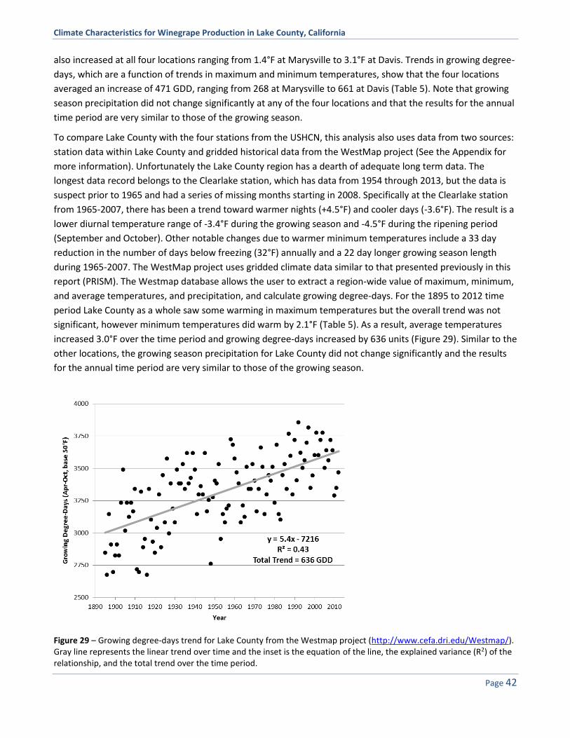
Climate Characteristics for Winegrape Production in Lake County, California
Page 42
also increased at all four locations ranging from 1.4°F at Marysville to 3.1°F at Davis. Trends in growing degree-
days, which are a function of trends in maximum and minimum temperatures, show that the four locations
averaged an increase of 471 GDD, ranging from 268 at Marysville to 661 at Davis (Table 5). Note that growing
season precipitation did not change significantly at any of the four locations and that the results for the annual
time period are very similar to those of the growing season.
To compare Lake County with the four stations from the USHCN, this analysis also uses data from two sources:
station data within Lake County and gridded historical data from the WestMap project (See the Appendix for
more information). Unfortunately the Lake County region has a dearth of adequate long term data. The
longest data record belongs to the Clearlake station, which has data from 1954 through 2013, but the data is
suspect prior to 1965 and had a series of missing months starting in 2008. Specifically at the Clearlake station
from 1965-2007, there has been a trend toward warmer nights (+4.5°F) and cooler days (-3.6°F). The result is a
lower diurnal temperature range of -3.4°F during the growing season and -4.5°F during the ripening period
(September and October). Other notable changes due to warmer minimum temperatures include a 33 day
reduction in the number of days below freezing (32°F) annually and a 22 day longer growing season length
during 1965-2007. The WestMap project uses gridded climate data similar to that presented previously in this
report (PRISM). The Westmap database allows the user to extract a region-wide value of maximum, minimum,
and average temperatures, and precipitation, and calculate growing degree-days. For the 1895 to 2012 time
period Lake County as a whole saw some warming in maximum temperatures but the overall trend was not
significant, however minimum temperatures did warm by 2.1°F (Table 5). As a result, average temperatures
increased 3.0°F over the time period and growing degree-days increased by 636 units (Figure 29). Similar to the
other locations, the growing season precipitation for Lake County did not change significantly and the results
for the annual time period are very similar to those of the growing season.
Figure 29 – Growing degree-days trend for Lake County from the Westmap project (http://www.cefa.dri.edu/Westmap/). Gray line represents the linear trend over time and the inset is the equation of the line, the explained variance (R2) of the relationship, and the total trend over the time period.

Climate Characteristics for Winegrape Production in Lake County, California
Page 43
Another way to examine change is by spatial differences between climate normal periods. Figure 30 shows the
1971-2000 period (left panel) and the preliminary 1981-2010 data (right panel) for the North Coast region of
California. The general patterns show differences in areas that have warmed and areas that have cooled. Some
cooling has occurred in the western central valley foothills of Yolo, Colusa, and Glenn counties, and some of
the mountainous areas in northern Lake County and Mendocino County. Areas of warming cover more of the
region with notable coastal and inland warming and slight to moderate warming across most of the
intermountain valleys where grapes are grown (Figure 30).
Figure 30 – North Coast of California average growing degree-days (F° units, Apr-Oct, base 50°F and no upper limit) for the 1971-2000 Climate Normals (left panel) and the preliminary 1981-2010 Climate Normals (right panel). Note that the class ranges mapped here corresponds to traditional Winkler Regions (Winkler et al. 1974) and updates to the lower Region I class found by Jones et al. (2010) and Hall and Jones (2010). (Data Source: Daly et al. 2008).
Conclusions The geography of wine is closely tied to climate. The climate structure of the various winegrowing regions
worldwide are critical determinants of the suitability of these regions to different winegrape cultivars, the
region’s overall productivity and potential wine style. While our understanding of the role climate structure
and suitability plays in viticulture and wine production is generally well developed, regional assessments of

Climate Characteristics for Winegrape Production in Lake County, California
Page 44
climate influences, risks, variability and trends is important to further our knowledge of how regional
suitability evolves over time. This report has examined these issues for the Lake County winegrowing region of
California.
Lake County is found in the intermountain region of Northern California approximately 100 miles north of San
Francisco and 30-50 miles from the coast (Figure 2). The county is centered on Clear Lake, the largest natural
freshwater lake in California, and is part of the chaparral and oak woodlands ecoregion found in the inland
landscapes surrounding much of the Central Valley. The region experiences a Mediterranean-like climate of
hot dry summers and cool moist winters.
Lake County has rich agricultural heritage starting with cattle operations in the early to mid-1800s and
followed by orchard operations that mainly included pears, walnuts, and plums for the prune market.
Vineyards were planted in the 1870s in numerous areas of the county and by the early 20th century the area
was earning a reputation for producing some of the world's best wines. However, similar to all other regions at
the time, Prohibition in 1920 ended Lake County's wine production. Most of the vineyards at the time were
ripped out and replanted with walnut and pear farms. A re-emergence of the wine industry began in the 1960s
when a few growers rediscovered the area's grape growing potential and began planting vineyards again.
From its early beginnings to today the wine industry in Lake County has grown to approximately 200 vineyards
representing nearly 8400 acres. The majority of the vineyards in the region are planted within seven TTB-
approved American Viticultural Areas (Figure 2). These AVAs encompass varying sizes and elevations of the
Lake County landscape providing a myriad of grape growing environments. The Guenoc Valley AVA in the
southern section of the county was the first AVA established in the county in 1981 and covers approximately
4200 acres of land at elevations that range from nearly 1000 to 1600 ft. Established in 1984, the Clear Lake
AVA is the largest AVA in the county at nearly 220000 acres, is centered over the lake, and has elevations that
range from 1300 ft. to nearly 4000 ft. The western-most, smallest and highest elevation region is the Benmore
Valley AVA, which was established in 1991 and contains 1450 acres of land with elevations from 2100 ft. to
nearly 2800 ft. The Red Hills Lake County AVA was approved in 2004 (with a minor boundary modification in
2013) and covers just over 32000 acres of land at elevations that range from close to 1300 ft. to over 3700 ft.
The High Valley AVA followed in 1985 and is largely a sub-AVA of the Clear Lake AVA, including over 17000
acres of land at elevations from 1300 ft. to just over 3300 ft. The most recently approved regions are the Big
Valley District Lake County AVA and the Kelsey Bench Lake County AVA which were both established in 2013.
The Big Valley District represents just over 11000 acres of land at elevations from nearly 1300 ft. to 1550 ft.
while the 9150 acre Kelsey Bench is found just upslope at elevations from nearly 1400 ft. to 1775 ft. (Figure 2).
Of the nearly 15000 acres planted to vines, walnuts, and pears in Lake County, vineyards make up
approximately 61% of the acreage. Growers have planted over 40 different winegrape varieties with bearing
acreage reported to represent approximately 65% red and 35% white varieties. The top seven varieties grown
make up approximately 90% of the acreage and include Cabernet Sauvignon, Sauvignon Blanc, Zinfandel,
Petite Sirah, Chardonnay, Merlot, and Syrah. In most years Cabernet Sauvignon and Sauvignon Blanc represent
50-70% of the production, with Cabernet Sauvignon representing 30-40% of the total and Sauvignon Blanc 20-
30%. Total production has varied from nearly 25000 to over 43000 tons during 2002-2013 with overall yields
ranging from 3.5-5.3 tons per acre. Red grape yields average 3.1-4.7 tons per acre while white grape yields are
higher at 4.3-6.30 tons per acre. While much of the fruit grown in Lake County is produced into wine outside
the region, more and more is being processed by the approximately 35 wineries within the region.

Climate Characteristics for Winegrape Production in Lake County, California
Page 45
From a weather and climate perspective, Lake County is influenced by its latitude and its location in the
westerly winds and the associated seasonality of storms coming off the Pacific. However, the strongest within
region influences are the distance from the Pacific Ocean, the moderate rain shadow effects of the coastal
mountains to the west, the landscape variations within the county, the moderating winds from Clear Lake, and
elevation differences. Combined these regional effects produce numerous microclimates within the county
that vary from other wine regions in the North Coast. The North Coast region receives from approximately 30
to greater than 60 inches of rainfall with regions to the north and along the coast experiencing the most.
Temperature extremes are low in the Lake County area, with absolute minimums below 20°F occurring
infrequently in the AVAs. Frost pressure is relatively low, with median last spring frosts from late March though
the third week in April. However, low-lying areas with less air flow and/or situated in isolated valleys, and
across portions of the Kelsey Bench, can experience frost into late May. Fall frosts are less of a concern as they
tend to occur long after harvest, ranging from late October into early December. As a result, the frost-free
period averages 195 to 248 days, sufficiently long in most years to fully ripen even late season varieties.
Maximum temperatures during the growing season peak from late July through early August with
approximately 15-25 days over 95°F each year, and absolute maximums that can reach over 100°F regularly.
The warm, dry summer results in evapotranspiration rates that climb to 0.20 inches per day by early May and
continuing through early September, requiring 18 inches or more of irrigation replenishment annually for the
average crop. However, winegrape ET values for the region have been reported to be from 4 to 12 inches
depending on the variety and year (McGourty et al. 2014). Wind flow patterns over the region are complex due
to landscape variations, but do tend to show relatively calm nighttime winds over the entire year and daytime
winds that pick up in and around Clear Lake and the surrounding landscapes, bringing afternoon breezes.
From a heat accumulation standpoint, values of growing degree-days (GDD) in Lake County vary mostly due to
elevation, but also generally increase as you head inland. The county as a whole averages 3215 GDD (1971-
2000 climate normals), while the seven AVAs average 3274. By AVA, the Big Valley District has the lowest
median of the seven regions, but is very similar to Benmore Valley, Kelsey Bench, and Clear Lake. The Red Hills
AVA has the highest median GDD and the lowest range between the coolest and warmest sites within the AVA.
GDD values such as those experienced in the Lake County range from a high Region II in the coolest zones
(2799 GDD) to high Region IV (3811 GDD) in the warmest zones of the Clear Lake AVA. For the AVA median
GDD values the area would be classed as mostly a Region III or very low Region IV. Simple average growing
season temperatures (April through October) over the Lake County AVAs average 65.3°F, ranging from 62.6°F
to 66.3°F. From these values the area would be classified as a largely Warm climate, with the ability to ripen a
range of varieties (e.g., Riesling, Chardonnay, Sauvignon Blanc, etc.) on the cooler sites, to ripening warmer
climate varieties such as Cabernet Sauvignon, Merlot, Syrah, Tempranillo, etc. on the warmer sites. Compared
to other wine regions regionally and worldwide, the Lake County AVAs fall in between the Alexander Valley
AVA and the Napa Valley AVA, and is similar to the average conditions found in the Douro Valley of Portugal
and the Chianti region of Italy.
Climate variability in the region can be large, with both vintage to vintage and decadal swings that are tied to
large scale atmospheric and oceanic interactions in the tropical Pacific (El Niño, La Niña and the Southern
Oscillation) and the North Pacific (Pacific Decadal Oscillation). By itself El Niño/La Niña tends to influence
mostly precipitation amounts over the western US, but can also play a minor role in seasonal temperature
variations. For the North Coast region of California, El Niño winters tend to be much wetter and slightly
warmer, while La Niña winters tend to be drier and cooler. While El Niño/La Niña is typically short-lived

Climate Characteristics for Winegrape Production in Lake County, California
Page 46
(seasonal to a few years) and receives much of the press, the Pacific Decadal Oscillation (PDO) is longer-lived
(decadal) and much more influential in wine region climates over the western US. During the positive PDO
phase the western North American fall, winter, and spring tends to be warmer and drier than average, while
during the negative PDO phase the region is colder and wetter. Research has found that when the negative
PDO (cold phase) is in place in combination with La Niña conditions, the North Coast experiences the coolest
springs with more spring frost, later frost events, and cooler growing seasons (e.g., 2009 and 2010).
Furthermore, when the negative PDO (cold phase) is in place in combination with neutral El Niño/La Niña
conditions (La Nada as often mentioned in the media), season to season variability becomes greater, typically
producing extremes in precipitation amounts (e.g., 2012-present).
Observations worldwide have shown that wine regions climates have changed over time and the trends in
temperatures have been related to vine growth, production, and wine characteristics through impacting
winter hardening potential, altering frost occurrence and growing season lengths, and increasing heat
accumulation and heat stress during the summer. California has seen changes in climate, but the nature of
these changes varies due to coastal versus inland and northern versus southern location differences. For
stations surrounding Lake County, trends from the 1890s through today show some locations trending greater
for maximum temperatures (Ukiah and Marysville), while others are trending more for minimum temperatures
(Davis and Healdsburg). Averaged over these four stations, average growing season temperatures have
increased 2.2°F since the 1890s while growing degree-days have increased 471 units. Precipitation does not
show significant trends for these locations. Within Lake County, Clearlake is the best long-term station and has
exhibited a trend toward warmer nights and cooler days, resulting in a lower diurnal temperature range during
the growing season and the ripening period (September and October). Other notable changes due to warmer
minimum temperatures include a 33 day reduction in the number of days below freezing (32°F) annually and a
22 day longer growing season length during 1965-2007. For Lake County as a whole, gridded climate data
shows a similar trend to the other regional stations with some warming in maximum temperatures but more
significant warming in minimum temperatures from 1985 to 2012. As a result, average temperatures increased
3.0°F over the time period and growing degree-days increased by 636 units for Lake County. Similar to the
other locations, growing season precipitation for Lake County did not change significantly and the results for
the annual time period are very similar to those of the growing season.
The Lake County region is a well-established winegrape growing region that is gaining more and more
recognition for quality fruit and wine production. The region’s history of viticulture has shown the potential to
ripen many cool to warm climate grape varieties. A long growing season with relatively low frost risk,
combined with high radiative potential due to elevation, moderately high diurnal temperature ranges and the
truncation of the growing season to cool nights during ripening make it a particularly attractive region to grow
winegrapes. Rapid growth of the industry is likely to continue due to current successes, diverse suitability, and
availability of land appropriate for growing quality winegrapes. Through the temporal and spatial analysis of
climate this research has hopefully helped to further characterize the structure and potential of grape growing
in region.
Acknowledgements Funding for this research was provided by the Lake County Winegrape Commission. I would like to thank Peter
Molnar, Debra Summerfield, and Sue Peters of the Lake County Winegrape Commission for all of their

Climate Characteristics for Winegrape Production in Lake County, California
Page 47
encouragement and support for this work. I would also like to thank Don Schukraft, of the Western Weather
Group for providing some of the climate data for the report.
References
Amerine, M. A. and A. J. Winkler. (1944). Composition and quality of musts and wines of California grapes.
Hilgardia, 15:493-675.
Amerine, M. A., H. W. Berg, R. E. Kunkee, C. S. Ough, V. L. Singleton, and A. D. Webb (1980). The Technology of
Wine Making, (4th ed.), AVI Publishing Company, Inc., Westport, Connecticut. 795 pp.
Anderson, J.D., Jones, G.V., Tait, A., Hall, A. and M.T.C. Trought (2012). Analysis of viticulture region climate
structure and suitability in New Zealand. International Journal of Vine and Wine Sciences, 46(3):149-165.
Carter, T. R., M. L. Parry, and J. H. Porter. (1991). Climatic change and future agroclimatic potential in Europe.
International Journal of Climatology. 11:251-269.
Code of Federal Regulations (2013): Alcohol, Tobacco Products, and Firearms (Title 27, Parts 1-646), Part 9 –
American Viticultural Areas, Subpart C - Approved American Viticultural Areas pp. 119-332.
Crespin, Y., M. LeBerre, and P. Uvietta. (1987). The system climate-vine-vinegrower: example of a dynamic
model. Bulletin de l’OIV, 60:5-26.
Daly, C., M. Halbleib, J.I. Smith, W.P. Gibson, M.K. Doggett, G.H. Taylor, J. Curtis, and P.A. Pasteris (2008).
Physiographically-sensitive mapping of temperature and precipitation across the conterminous United
States. International Journal of Climatology, 28(15):2031-2064.
Easterling, D. R. et al. (2000). Observed variability and trends in extreme climate events: A brief review, Bull.
Am. Meteorol. Soc. 81, 417-425.
Frauenfeld O.W., Davis R.E., Mann M.E. (2005) A distinctly interdecadal signal of Pacific Ocean–Atmosphere
interaction. J Clim 18:1709–1718
Gladstones, J., (1992). Viticulture and Environment. WineTitles: Adelaide, Australia, 310 p.
Griffith, G.E., Omernik, J.M., Smith, D.W., Cook, T.D., Tallyn, E., Moseley, K., and Johnson, C.B., (2011 draft),
Ecoregions of California (color poster with map, descriptive text, and photographs): Menlo Park, California,
U.S. Geological Survey (map scale 1:1,100,000).
Hall, A. and G.V. Jones (2010). Spatial analysis of climate in winegrape growing regions in Australia. Australian
Journal of Grape and Wine Research, 16:389-404.
IPCC (2007). Alley R. et al. Climate Change 2007: The Physical Science Basis. Summary for Policymakers.
Contribution of the Working Group I to the Fourth Assessment of the Intergovernmental Panel on Climate
Change. IPCC Secretariat (http://www.ipcc.ch/).
Jones, G.V. (1997). A Synoptic Climatological Assessment of Viticultural Phenology. Dissertation, University of
Virginia, Department of Environmental Sciences, 394 pp.
Jones, G.V., (2005). Climate change in the western United States grape growing regions. Acta Horticulturae
(ISHS), 689:41-60.
Climate Characteristics for Winegrape Production in Lake County, California
Page 48
Jones, G.V. (2006). Climate and Terroir: Impacts of Climate Variability and Change on Wine. In Fine Wine and
Terroir - The Geoscience Perspective. Macqueen, R. W., and L. D. Meinert, (eds.), Geoscience Canada
Reprint Series Number 9, Geological Association of Canada, St. John's, Newfoundland, 247 pages.
Jones, G.V. and Davis, R.E. (2000). Using A Synoptic Climatological Approach to Understand Climate/Viticulture
Relationships, International Journal of Climatology, 20:813-837.
Jones, G.V. and E. Hellman. (2003). Site Assessment: in “Oregon Viticulture” Hellman, E. (ed.), 5th Edition,
Oregon State University Press, Corvallis, Oregon, p 44-50.
Jones, G.V. and Goodrich, G.B., (2008). Influence of Climate Variability on Wine Region in the Western USA and
on Wine Quality in the Napa Valley. Climate Research, 35: 241-254.
Jones, G.V. and Webb, L.B. (2010). Climate Change, Viticulture, and Wine: Challenges and Opportunities.
Journal of Wine Research, 21: 2(103-106).
Jones, G.V., M. A. White, O. R. Cooper, and K. Storchmann. (2005). Climate Change and Global Wine Quality.
Climatic Change, 73(3): 319-343.
Jones, G.V., M. Moriondo, B. Bois, A. Hall, and A. Duff. (2009). Analysis of the spatial climate structure in
viticulture regions worldwide. Le Bulletin de l'OIV 82(944,945,946):507-518.
Jones, G.V., Duff, A.A., Hall, A. and Myers, J.W., (2010). Spatial analysis of climate in winegrape growing regions
in the western United States. American Journal of Enology and Viticulture, 61(3), 313-326.
Jones, G.V., Reid, R., and A. Vilks (2012). Climate, Grapes, and Wine: Structure and Suitability in a Variable and
Changing Climate pp 109-133 in The Geography of Wine: Regions, Terrior, and Techniques, edited by P.
Dougherty. Springer Press, 255 pp.
Karl, T. R., P. D. Jones, R. W. Knight, G. Kukla, N. Plummer, V. Razuvayev, K. P. Gallo, J. Lindseay, R. J. Charlson
and T. C. Peterson. (1993). A new perspective on global warming: asymmetric trends of daily maximum
and minimum temperature. Bulletin of the American Meteorological Society, 74:1007–1023.
Kliewer, W. M. and R. E. Torres. (1972). Effect of controlled day and night temperatures on grape coloration.
American Journal of Enology and Viticulture, 23:71-77.
Lake County Department of Agriculture (2003-2013): Crop Reports. Steve Hajik, Agricultural Commissioner.
Mantua N.J., and Hare S.R. (2002). The Pacific Decadal Oscillation. J Oceanogr 58:35–44.
Matthews, M. A. and M. M. Anderson. (1988). Fruit ripening in Vitis vinifera L.: responses to seasonal water
deficits. American Journal of Enology and Viticulture, 39(4):313-320.
McGourty, G., Keiffer, R., and B. Zoller. (2014). Vineyard Water Use in Lake County, California. University of
California Agriculture and Natural Resources. UC Cooperative Extension document.
McIntyre, G. N., L. A. Lider, and N. L. Ferrari. (1982). The chronological classification of grapevine phenology,
Amer. J. Enology and Viticulture, 33(2):80-85.
McMaster, G.S., and W. Wilhelm. (1997). Growing degree-days: one equation, two interpretations. Agric.
Forest Meteorol. 87(4):291-300.
Menne, M. J., Williams, Jr., C. N., and R. S. Vose, (2013). United States Historical Climatology Network Daily
Temperature, Precipitation, and Snow Data. Carbon Dioxide Information Analysis Center, Oak Ridge
National Laboratory, Oak Ridge, Tennessee.

Climate Characteristics for Winegrape Production in Lake County, California
Page 49
Moonen, A. C., L. Ercoli, M. Mariotti, and A. Masoni. (2002). Climate change in Italy indicated by
agrometeorological indices over 122 years. Agricultural and Forest Meteorology. 111:13-27.
Mori, K., Sugaya, S. and H. Gemma. (2005). Decreased anthocyanin biosynthesis in grape berries grown under
elevated night temperature condition. Scientia Horticulturae, 105:319-330.
Mullins, M. G., A. Bouquet, and L. E. Williams. (1992). Biology of the Grapevine, Cambridge University Press,
Great Britain. 239 pp.
Nemani, R.R., White, M.A., Cayan, D.R., Jones, G.V., Running, S.W., and J.C. Coughlan, (2001). Asymmetric
climatic warming improves California vintages. Climate Research, Nov. 22, 19(1):25-34.
Prescott, J. A. (1965). The climatology of the vine (Vitis Vinifera L.) the cool limits of cultivation. Transcriptions
of the Royal Society of Southern Australia, 89:5-23.
Schultz, H.R. and Jones, G.V. (2010). Climate Induced Historic and Future Changes in Viticulture. Journal of
Wine Research, 21:2(137-145).
Smart, R. E. and P. R. Dry. (1980). A climatic classification for Australian viticultural regions: Australian
Grapegrower and Winemaker, 17:8-16.
U.S. Environmental Protection Agency (2000). Level III ecoregions of the continental United States (revision of
Omernik, 1987): Corvallis, Oregon, USEPA – National Health and Environmental Effects Research
Laboratory, Map M-1, various scales.
Western Regional Climate Center (WRCC, 2013), National Oceanic and Atmospheric Administration (NOAA),
Reno, NV –http://www.wrcc.sage.dri.edu/
Williams, L. E. (2000). Grapevine water relations. In: L.P. Christensen (ed.) Raisin Production Manual. DANR
Publications, Univ. California, Oakland, CA. pp. 121-126.
Winkler, A. J., Cook, J. A., Kliewer, W. M. and Lider, L. A., (1974). General Viticulture, (4th ed.), University of
California Press, Berkeley. 740 pp.
Appendix
Data and Methods
Ecoregions One of the most common and useful means to categorize the landscapes of the United States is through the
dominant ecoregion (Omernik et al. 2000; Griffith et al. 2011). Ecoregions denote and describe regions with
general similarities in the type, quality, and quantity of environmental resources which in turn provide a means
for research, assessment, management, and monitoring of ecosystems by federal, state and local agencies.
Ecoregions for the United States have been developed based upon the spatial patterns and composition of
biotic and abiotic phenomena including geology, physiography, vegetation, climate, soils, land use, wildlife,
and hydrology. These ecoregions vary from the coarse, national scale Level I (15 regions) to the finer, regional
scale Level IV regions (hundreds of regions) (USEPA, 2000).

Climate Characteristics for Winegrape Production in Lake County, California
Page 50
Weather and Climate Various sources of climate data were used in this assessment and include:
PRISM
To characterize and depict the spatial climate characteristics in the North Coast and Lake County AVAs this
assessment utilizes a climate dataset called PRISM (Parameter-elevation Relationships on Independent Slopes
Model) that is the official spatial climate data set of the United States Department of Agriculture (Daly et al.
2008). The 1971-2000 climate normals data are created as 15 arc-second (~400 m, 1312 ft.) grids through an
interpolation method that reflects the current state of knowledge of spatial climate patterns in the United
States. In general, PRISM calculates a climate-elevation regression for each digital elevation model (DEM) grid
cell, and stations entering the regression are assigned weights based primarily on the physiographic similarity
of the station to the grid cell.
PRISM takes into account the location, elevation, coastal proximity, topographic facet orientation (aspect),
vertical atmospheric layer, topographic position, and orographic effectiveness of the terrain. The PRISM grids
are constructed from a comprehensive collection of stations from many networks, including the National
Weather Service Cooperative Network, USDA Snow Telemetry, US Forest Service Remote Automatic Weather
Stations, local networks, snow courses, and others (16615 precipitation sites and over 11500 temperature sites
were used in the United States). In addition to the dense station network, the PRISM data set underwent a
comprehensive peer review procedure that incorporated local knowledge and data into the development
process. Furthermore, PRISM has been validated using remote vineyard locations (Jones unpublished data),
successfully applied in viticulture zoning studies (Jones et al. 2004; Jones et al. 2006), and used by Jones et al.
(2010) to characterize the climate of each of 135 AVAs in the western United States.
The PRISM climate data used in this report include monthly precipitation, maximum and minimum
temperatures, and the median dates of the first fall and last spring frosts (www.prism.oregonstate.edu/).
Caveats with the PRISM data are that it is clearly a model and estimates the climate parameters over the
landscape using known relationships between topography and climate. As such, unique local conditions could
cause the model to over or under estimate the climate grids, but large discrepancies are not expected due to
the strong validation and quality control of the data (Daly et al., 2008). While the PRISM data is the highest
resolution climate data product in the United States and is the USDA standard, the resolution of approximately
16 hectares is such that capturing the exact within site or block variations in GDD and frost potential is difficult.
USHCN
The longest term climate data available in the US is the United States Historical Climatology Network (USHCN),
which is a subset of the U.S. Cooperative Observer Network operated by NOAA's National Weather Service
(NWS). The approximately 1200 USHCN stations were originally selected according to factors such as record
longevity, percentage of missing values, spatial coverage as well as the number of station moves and/or other
station changes that may affect data quality. Most USHCN stations are situated in rural areas or small towns;
however, a smaller number of stations are also part of the NOAA NWS synoptic network, whose stations are
generally located at airports in more urbanized environments (Menne et al. 2013).
Unfortunately there are no qualified stations within Lake County in the USHCN database. However, four
stations surrounding the region have monthly data that covers the 1893 to 2012 time period: Ukiah,
Marysville, Davis, and Healdsburg and are used for comparative purposes with other Lake County data.
Climate Characteristics for Winegrape Production in Lake County, California
Page 51
WRCC & Westmap
The US Regional Climate Centers (RCC) deliver climate services at national, regional and state levels working
with NOAA partners in the National Climatic Data Center, National Weather Service, the American Association
of State Climatologists, the Regional Sciences and Assessment Program, and other NOAA Research Institutes.
The WRCC also partners with the Department of Interior Climate Science Centers and Landscape Conservation
Cooperatives and is administered by the National Oceanic and Atmospheric Administration. Specific oversight
is provided by the National Climatic Data Center (NCDC) of the National Environmental Satellite, Data, and
Information Service (NESDIS). For this assessment data and information was accessed from the Western
Regional Climate Center ([email protected]) and includes long-term daily and monthly data for the Clearlake 4 SE
COOP station (041806) along with summary statistics on extremes. Additional monthly data for the Lakeport
station (044701) was used to summarize precipitation.
Clearlake 4 SE, 1350 ft. in elevation at 38° 54'N and 122° 36'W
Lakeport, 1340 ft. in elevation at 39° 02'N and 122° 55'W
To compare Lake County with the four stations from the USHCN (see above), this analysis uses data from
WestMap project (www.cefa.dri.edu/Westmap/), using gridded climate data (PRISM) similar to that presented
previously in this report. WestMap is the Western Climate Mapping Initiative, a collaborative effort being
undertaken by the WestMap Consortium. The WestMap Consortium is a group of stakeholders from public and
private sectors who share a common interest in regional climate variability and fine-scale mapping of this
climate. The initial fundamental data that went into Westmap is monthly PRISM temperature (maximum,
mean, minimum) and precipitation at 4 km resolution and the period of record is 1895 to the present. The
Westmap database allows the user to extract a region-wide (county, climate division, state, etc.) value of
maximum, minimum, and average temperatures, and precipitation, and calculate growing degree-days.
Western Weather Group
To augment the long term climate station data from the USHCN and the WRCC (see above), this report uses
data from a network of stations managed by the Western Weather Group (WWG). The WWG is a team of
scientists working with others in agriculture, industry, power generation, recreation and consulting to address
their weather risks with both weather and climate product solutions. They also supply and install industrial
grade meteorological and environmental monitoring systems and custom weather forecasting services.
Furthermore they incorporate data from automated weather stations into weather forecasts and other useful
products (www.westernweathergroup.com).
In Lake County the Winegrape Commission has worked with WWG to develop a network of 12 stations in the
county and WWG augments the stations with a few others just outside the county, to provide the wine
industry and others daily to weekly to annual summaries along with forecast products.
For this report, WWG supplied hourly and daily data for four stations for various time periods from 2005
through 2013. Hourly data for a six year period from 2008-2013 was used to develop wind roses for Kelseyville,
Red Hills, Upper Lake, and Guenoc Valley (See list below and Figure 1 for station locations). Wind roses are
diagrams that use hourly wind-speed and wind-direction data to construct a frequency histogram of wind
speed data in polar coordinates that correspond to the wind direction with bars that indicate both frequency

Climate Characteristics for Winegrape Production in Lake County, California
Page 52
and speed. For this report wind roses were created for the six year period for daytime (8am to 8 pm) and
nighttime (8pm to 8am) along with summary statistics and a table of frequencies.
Kelseyville, 1386 ft. in elevation, 39° 00' 22"N and 122° 50' 47"W
Upper Lake, 1377 ft. in elevation, 39° 10' 08.5"N and 122º 55' 06.2"W
Red Hills, 2000 ft. in elevation, 38° 54' 52"N and 122° 43' 58"W
Guenoc Valley, 950 ft. in elevation, 38° 44' 28"N and 122° 30' 50"W
Daily data from WWG was used to develop climatology of evapotranspiration (ET). ET is the loss of water to
the atmosphere by the combined processes of evaporation (from soil and plant surfaces) and transpiration
(from plant tissues). It is an indicator of how much water crops or other vegetated surfaces need for healthy
growth and productivity. Three of the stations had daily ‘reference’ crop evapotranspiration (ETo), which is
typically either grass or alfalfa surfaces whose biophysical characteristics have been studied extensively. For an
annual daily summary of ETo this report used Kelseyville during 2005-2009, Red Hills during 2006-2010, and
Guenoc Valley during 2005-2009 (See Figure 1 for station locations). Daily ETo values were averaged over the
five year period for each station to produce the annual climatology.
ETCCDI
Of course quality control is an important aspect of analyzing climate station data. Climate data are the records
of observed climate conditions taken at specific sites and times with particular instruments under a set of
standard procedures. A climate dataset therefore contains climate information at the observation sites, as well
as other non-climate-related factors such as the environment of the observation station, and information
about the instruments and observation procedures under which the records were taken. An assumption is
made that the station records are representative of climate conditions over a region when the data are used in
climate analysis. This is, unfortunately, not always the case (Peterson et al. 1998). Station moves, instrument
changes, calibration issues, recorder errors, etc. can all cause issues with climate station data. To account for
potential issues with station data, numerous tools have been developed to manage and/or correct these
issues. This climate assessment uses one such tool created by the CCI/CLIVAR/JCOMM Expert Team (ET) on
Climate Change Detection and Indices (ETCCDI). The main goal of the tool is to check for data homogeneity and
the quality control of outliers (unrealistic values, bad data points, etc.). The aim of climate data
homogenization is to adjust observations, if necessary, so that the temporal variations in the adjusted data are
caused only by climate processes. An authoritative review on climate data homogenization can be found in
Peterson et al. (1998).
The CCI/CLIVAR/JCOMM Expert Team (ET) on Climate Change Detection and Indices (ETCCDI) has also
developed a suite of indices for understanding the behavior of climate at a given station (Karl et al. 1999; Wang
et al. 2003; Peterson 2005). The analysis of average climate conditions, while important, may not be as critical
as understanding the change in the frequency or severity of extreme climate events. However, little
standardization of appropriate indices for developing a global picture of conditions and trends has been done
until ETCCDI developed a suite of 27 core indices. These indices provide a common framework by which the
frequency or severity of extreme climate events can be assessed worldwide. Therefore, the 27 indices are
Climate Characteristics for Winegrape Production in Lake County, California
Page 53
calculated for the Clearlake station for 1954-2007 after data quality control and homogenization has been
properly assessed. Only those index values with significant trends are reported here.
Calculating and Using Degree-Days
The use of climate to describe and/or compare regions within the US and worldwide is inadequate and mostly
inappropriately done (Jones et al. 2010). The numerous issues concerning the comparison of climate indices
from other sources results from the historic use of station data, using data from different time periods, and
using different methods of calculating the indices, especially degree-days. While many governments and
organizations recognize the 30 year climate normal period (1971-2000) as the standard (e.g., the World
Meteorological Organization), not all published climate data (e.g., temperatures, degree-days, etc.) is
summarized similarly. Some data may include the entire period of record (i.e., tens of years to over a hundred
years), while others might include a shorter subset of years. Using the same time period is important, as both
climate variability and trends will result in changes in the statistical distribution of the data. For example, in the
western United States GST and GDD have standard deviations of 1.3-2.2°F and 200-400 units, respectively
(Jones and Goodrich 2008). However, the variability over differing time periods can vary by as much as 50%
depending on the length of the data record. In addition, warming trends in GST and GDD in the western US
during 1948-2004 have been 1.6-3.1°F and 200-600 units, respectively, revealing how important it is to know
the time period the climate indices represent (Jones 2005, Jones and Goodrich 2008).
As an example, Jones et al. (2010) compared their results with the map and data originally published
by Winkler et al. (1974; their Figure 12 and Table 3, pages 62-66). The comparison reveals some significant
differences due to the use of stations, the time period of the data used, and the available mapping technology
used at the time. First, Winkler et al. (1974) used data from multiple sources without specifying the time
period of the data or the exact method of calculation for the degree-days reported (i.e., simple average GDD,
and daily, multi-day, or monthly formulations). These issues alone make the comparison of the values less than
ideal. Second, the use of individual stations and the construction of a map from the few sites in each region
resulted in a more or less correct general depiction of the climate in California at the time but with marginal
accuracy (Winkler et al. 1974; their Figure 12). Winkler et al. (1974) showed that broad areas have similar
levels of suitability, whereas the spatial data used in Jones et al. (2010) and this Lake County report depicts
much more pronounced within-region variation. Third, using published data from a sample of 30 stations
across the western United States given by Winkler et al. (1974; their Table 3) reveal GDD values across the
stations that are 300 units or 10% less on average (a range of 3 to 23% across the 30 stations) than the same
stations from the 1971-2000 climate normals (Western Regional Climate Center; www.wrcc.dri.edu). Changes
in climate such as this example and others (Jones 2005) highlight the need to use values from a current and
similar time period to properly compare wine region climates.
Another important issue in considering comparable climate information comes from how the data was
averaged (i.e., hourly, daily, or monthly). While the advent of better weather station instrumentation and
software to calculate climate indices has helped many develop their own site-specific data from hourly or
shorter time periods, often this data is compared to historical information that comes from daily maximum
and minimum observations or monthly data. Hourly data, which arguably better reflects the true thermal
effects on the crops, results in heat accumulation values that tend to be lower than both daily and monthly
approximations, while monthly data can slightly underestimate heat accumulation during the first and last

Climate Characteristics for Winegrape Production in Lake County, California
Page 54
months of the growing season (Jones et al. 2010). Therefore, one must be careful to compare similar time
period averaged data. Furthermore, the use of readily accessible daily maximum and minimum temperature
data to derive heat accumulation values has been criticized for not representing the diurnal structure of
temperature (Jones et al. 2012). Various methods have been proposed (e.g., sine wave, triangle, etc.) to
improve the simple averaging method and have achieved some success. However, these methods 1) do not
produce tremendous differences in heat accumulation indices that would affect general suitability studies for
viticulture, 2) are much more applicable for scientific field applications such as phenological modeling, 3) are
not readily available or user friendly for the average grape grower, and 4) are not comparable to commonly
published climate index values.
Another significant methodological difference exists between simple average growing degree-days
formulations that are standard practice in viticulture studies (Winkler et al. 1974, Gladstones 1992, Jones
2006) versus the so-called ‘corn’ degree-days (McMaster and Wilhelm 1997). The main difference is in how the
base temperature is dealt with in the formula. For the simple average method any day with an average
temperature below the base of 50°F for winegrapes, there is no accumulation. The ‘corn’ degree-day method,
however, adjusts all minimum temperatures to the base, therefore artificially adjusting the average
temperature and resulting in spring and fall monthly values 50-400% higher than simple average degree-days
or April-October total accumulations 28-33% higher. Calculations for a sample of wine regions in the western
US found the ‘corn’ degree-day formulation to be 10-15% higher than the simple average formulation (Jones et
al. 2010). Furthermore, while ‘corn’ degree-days may be the standard for broadacre crops (McMaster and
Wilhelm 1997), ‘corn’ degree-days have a set upper limit of 86°F, which along with artificially adjusting the
base temperature, may or may not be appropriate for winegrapes (see below) and is not commonly applied in
historic degree-day calculations for viticulture (Jones 2006). Furthermore, because the ‘corn’ method has been
implemented in many pieces of weather station software (e.g., HOBOware, Onset Computer Corporation) it
can confound any comparison with published data using the simple average method.
While Winkler et al. (1974) and McIntyre et al. (1987) have both suggested that refinements to
understanding wine region climate indices are needed; no large scale work in this area has been attempted.
Additional issues that need to be addressed through research include optimizing the lower and upper
temperature thresholds for degree-day formulations. While these thresholds have typically been defined by
their influence on phenological event timing, they are commonly derived from photosynthetic activity limits.
For example, in terms of the lower temperature threshold, research has shown that very little photosynthesis
occurs in grapevine leaves when temperatures are below 41°F (Mullins et al. 1992). Furthermore, while other
research has found strong evidence for a 40-41°F base temperature for grapevines in Australia and Europe,
little has been done to confirm these thresholds across other wine regions and for a wider range of varieties
(Jones et al. 2012). In addition, from the discussion of ‘early’ versus ‘late’ budding varieties (Winkler et al.
1974), the base temperature threshold for accumulation is likely strongly cultivar specific. There is also some
evidence that grapevines have a maximum temperature threshold of approximately 90 to 95°F (Jones et al.
2012), however others have found that optimum net photosynthesis occurs over a wide range of temperature
(77-95°F), making it difficult to pinpoint a universal upper temperature threshold.
The development of any index also requires the creation of classes for distinguishing between
categories. Two important issues involved in the classification of quantitative data include the number of
classes and the specific way the data is divided. These decisions are important for depicting climate indices for
viticulture suitability because they can include or exclude sites/regions and are often being based upon

Climate Characteristics for Winegrape Production in Lake County, California
Page 55
convenience (i.e., rounded numbers). For example, Amerine and Winkler (1944, p 504) specified their five
‘region’ concept in order to “reduce the size of the tables and differentiate among the recommendations”, not
necessarily to provide clear demarcations between climate class suitability. In addition, the classes specified by
these authors did not give specific lower and upper limits to Regions I and V, respectively. The authors only
mentioned that the limits appear to be 950 and 2778 based upon anecdotal evidence from a short list of
climate stations worldwide, not stations in the western US or California. Jones et al. (2010), Anderson et al.
(2012) and others have shown that the lower limit for viticulture is 1500 GDD (WI Region I). Furthermore, this
same research in the western US, New Zealand, and Europe (Jones et al. 2012) has shown that the WI Region I
should be split into a Region Ia (1500-2000, hybrid and only the earliest ripening V. Vinifera) and Region Ib
(2000-2500, later ripening hybrid and most cool climate V. Vinifera) to better discriminate sufficiently between
cooler climate zones. Jones et al. (2010 and 2012) also found an upper limit of 4900 GDD (WI Region V) based
on the spatial climate characteristics of the warmest V. Vinifera growing zones worldwide, including the
Madera AVA in the central valley of California. Finally, the class limits applied to climate indices should be
thought of as general demarcations between broad ‘regions’ or maturity groups whereby some varieties
clearly overlap from one class type to another (e.g., GST maturity classes; Jones 2006).
Take home messages with using degree-days:
1) When comparing growing degree-day numbers from any source know the;
a) Time period of the data and preferably use a common 30 year climate normal period.
b) Time interval, is the data from hourly, daily, or monthly observations or averaging. Always use the
same interval.
c) Months that the data is accumulated over, the norm is April through October (Northern
Hemisphere) even if
d) Base temperature used in the calculation, 50°F is the norm, whether it is the correct value or not
for that variety.
e) If an upper cut-off is used, this commonly occurs with either weather software or web tools that
may not specify the form being used.

Climate Characteristics for Winegrape Production in Lake County, California
Page 56
Appendix Table 1 – Selected California American Viticultural Area (AVA) from Jones et al. (2010). Shown are total
area (acres), elevation statistics (feet), and 1971-2000 quantile statistics for the growing season average temperature (GSTavg) and growing degree-days (GDD) that occur spatially over the AVAs.
AVA Name Area1
(acres)
Elevation (ft) GSTavg (°F) GDD
Median Max Min Range Min 25% Median 75% Max Min 25% Median 75% Max
Alexander Valley 78300 485 2447 157 2289 62.7 64.3 64.6 65.0 66.4 2738 3069 3134 3213 3523
Anderson Valley 58300 712 1758 197 1561 60.5 61.8 62.9 63.7 64.9 2257 2520 2759 2934 3191
Atlas Peak 12400 1512 2470 856 1614 62.1 63.9 64.5 64.8 66.6 2601 2983 3098 3164 3562
Benmore Valley 1400 2598 2795 2116 679 64.7 65.1 65.1 65.2 65.5 3155 3242 3248 3257 3332
Bennett Valley 8300 705 1568 249 1319 62.3 63.2 63.3 63.6 64.3 2637 2831 2860 2909 3069
Big Valley District 11300 1355 1551 1328 223 64.8 64.9 65.0 65.1 65.4 3171 3230 3245 3253 3281
Calistoga 12800 469 1273 282 991 64.9 65.7 66.0 66.2 66.4 3193 3362 3422 3467 3517
Capay Valley 99100 1007 2926 197 2729 63.8 67.4 68.0 69.0 70.1 2963 3730 3866 4065 4318
Central Coast 5473400 1066 5478 0 5478 55.7 61.7 64.1 65.8 70.7 1213 2516 3019 3379 4444
Chalk Hill 22600 338 403 338 66 62.9 63.4 63.7 64.1 65.8 2768 2882 2941 3029 3386
Chalone 7700 1574 1981 1092 889 63.7 64.1 64.3 64.4 65.5 2939 3031 3061 3091 3328
Chiles Valley 6400 1027 1633 797 836 64.1 65.0 65.5 66.0 66.6 3019 3222 3312 3429 3555
Clear Lake 219200 1548 3956 1309 2647 63.1 65.0 65.2 66.0 67.8 2799 3209 3267 3442 3811
Cole Ranch 200 1555 1719 1496 223 64.3 64.3 64.4 64.5 64.5 3062 3065 3084 3103 3103
Covelo 40000 1597 2699 1397 1302 62.9 63.8 64.1 64.5 65.2 2772 2965 3020 3101 3258
Diamond Mountain 5000 1004 2083 531 1551 63.8 65.3 65.6 65.9 66.3 2952 3272 3343 3409 3501
Dos Rios 16700 1460 2726 823 1902 63.3 63.7 63.8 64.0 65.4 2848 2929 2963 3002 3308
Dry Creek Valley 77900 794 2326 82 2244 62.2 64.1 64.5 64.8 65.3 2617 3020 3103 3163 3280
Dunnigan Hills 67000 197 400 46 354 69.1 69.6 69.7 69.8 70.3 4093 4192 4217 4243 4343
Edna Valley 24200 279 692 131 561 59.4 60.6 60.9 61.3 63.0 2005 2279 2344 2411 2785
El Dorado 408800 2375 4992 528 4464 61.8 65.1 65.9 66.5 68.8 2574 3238 3416 3546 4037
Fair Play 23200 2211 3385 1647 1738 65.7 65.8 66.0 66.0 66.0 3375 3391 3422 3434 3438
Fiddletown 12100 1801 2411 1246 1164 65.9 66.2 66.3 66.4 66.8 3411 3474 3496 3526 3602
Guenoc Valley 4200 1059 1581 974 607 66.0 66.2 66.2 66.7 67.7 3420 3465 3481 3580 3796
Hames Valley 12300 768 1227 561 666 65.8 66.5 66.9 67.2 67.6 3384 3544 3632 3685 3778
High Valley 17200 1971 3339 1332 2007 64.6 66.1 66.5 66.9 67.5 3139 3447 3548 3618 3755
Howell Mountain 13100 1745 2552 1027 1525 63.5 63.9 64.1 64.4 66.5 2894 2986 3015 3092 3537
Kelsey Bench 9200 1519 1775 1384 391 64.9 65.1 65.2 65.3 66.2 3189 3210 3250 3325 3593
Knights Valley 37300 843 3890 213 3677 58.5 63.8 65.0 65.3 66.5 1903 2959 3218 3287 3541
Livermore Valley 238700 768 3372 171 3201 61.7 64.4 64.9 65.4 68.4 2502 3092 3193 3296 3935
Lodi 542200 79 495 0 499 67.9 68.3 68.6 68.7 69.2 3839 3915 3980 4005 4122
Los Carneros 37400 95 1246 0 1246 62.6 63.4 63.8 64.3 67.0 2695 2867 2947 3069 3649
Madera 457200 213 485 125 361 70.2 70.6 71.1 71.3 72.6 4336 4410 4520 4567 4835
McDowell Valley 2200 804 1036 604 433 64.6 65.0 65.1 65.2 65.4 3134 3217 3244 3269 3305
Mendocino 176700 1230 3736 407 3329 62.5 64.4 64.9 65.3 67.2 2680 3083 3193 3283 3683
Mendocino Ridge 83900 1407 2558 459 2099 59.1 61.6 62.6 63.0 64.3 1951 2479 2701 2795 3069
Monterey 603200 377 2568 0 2568 57.2 60.6 62.1 64.3 68.0 1541 2275 2594 3058 3861
Mount Harlan 7800 2342 3047 1430 1617 60.6 61.3 62.5 63.2 64.2 2273 2416 2687 2835 3035

Climate Characteristics for Winegrape Production in Lake County, California
Page 57
Appendix Table 1 Continued:
AVA Name Area1
(acres)
Elevation (ft) GSTavg (°F) GDD
Median Max Min Range Min 25% Median 75% Max Min 25% Median 75% Max
Mt. Veeder 17000 1115 2549 367 2181 61.5 64.9 65.7 66.2 67.1 2468 3186 3370 3465 3667
Napa Valley 401100 813 3854 0 3854 59.2 64.7 65.8 66.5 68.8 2036 3155 3389 3546 4023
North Coast 3269500 981 5330 0 5330 53.4 62.4 63.7 65.0 68.8 736 2655 2938 3224 4034
North Yuba 22200 1738 2758 646 2112 64.7 66.3 66.6 67.3 70.3 3146 3487 3564 3704 4345
Northern Sonoma 323200 633 3890 82 3808 58.5 62.9 64.0 64.7 66.5 1903 2758 3002 3157 3541
Oak Knoll District 9900 92 886 23 863 64.2 64.8 65.2 65.5 66.3 3040 3170 3253 3312 3501
Oakville 6900 167 912 157 754 65.1 65.9 66.0 66.2 66.7 3240 3410 3434 3479 3584
Pacheco Pass 9200 390 1404 144 1260 63.4 64.5 64.9 65.2 65.8 2880 3105 3193 3267 3386
Paso Robles 608700 1305 2444 577 1866 61.4 64.9 66.0 66.6 68.3 2450 3202 3425 3560 3919
Potter Valley 29000 1155 3021 892 2129 63.0 63.9 64.3 65.0 65.3 2779 2981 3076 3206 3278
Red Hills Lake County 31000 2037 3611 1381 2230 64.5 66.0 66.8 67.2 67.6 3114 3434 3596 3683 3776
Redwood Valley 32200 1148 2404 797 1607 62.5 63.6 64.2 65.0 65.5 2675 2916 3035 3211 3332
Rockpile 14700 1401 2227 800 1427 63.8 64.2 64.3 64.5 65.2 2952 3044 3074 3116 3254
Russian River Valley 156000 203 1437 49 1387 61.3 62.5 62.8 62.9 65.1 2425 2686 2736 2770 3233
Rutherford 7500 180 912 157 754 65.7 65.8 65.9 66.1 66.7 3364 3388 3411 3449 3575
San Francisco Bay 1894600 554 3506 0 3506 57.0 62.2 63.5 64.4 68.3 1494 2608 2894 3091 3924
San Ysidro District 2500 223 367 157 210 63.9 64.9 65.5 65.8 65.9 2974 3200 3328 3382 3402
Santa Clara Valley 318700 223 1456 0 1456 62.7 63.9 64.3 64.6 66.1 2729 2974 3069 3125 3445
Santa Cruz Mountains 410300 1105 3506 16 3490 57.7 62.2 63.0 63.7 65.3 1643 2610 2795 2930 3281
Santa Maria Valley 102700 771 2936 210 2726 59.8 61.3 62.8 65.1 68.8 2095 2412 2732 3242 4025
Santa Rita Hills 33400 544 1512 194 1319 61.0 62.2 62.6 62.9 66.3 2365 2619 2693 2758 3488
Santa Ynez Valley 181800 863 2982 197 2785 61.0 62.8 63.3 65.7 69.5 2365 2734 2844 3364 4174
Shenandoah Valley 13300 1450 1968 820 1148 66.0 66.5 66.9 67.2 67.9 3438 3537 3616 3685 3845
Sierra Foothills 2669300 1542 5579 177 5402 57.5 66.2 67.6 68.6 72.8 1814 3467 3776 3992 4892
Solano Co Green Valley 14000 453 2011 16 1994 64.9 66.7 67.5 68.1 68.8 3202 3568 3746 3868 4021
Sonoma Co Green Valley 19100 289 810 92 718 61.9 62.5 62.6 62.6 62.9 2560 2669 2693 2707 2774
Sonoma Coast 524600 249 2145 0 2145 54.0 60.7 62.1 62.9 65.9 850 2304 2596 2754 3404
Sonoma Mountain 5800 876 1784 479 1305 63.3 64.6 65.1 65.5 65.9 2848 3125 3245 3311 3404
Sonoma Valley 116100 738 2398 0 2398 61.5 63.4 64.1 64.7 66.0 2468 2878 3017 3139 3431
South Coast 2116000 810 5448 0 5448 61.4 66.5 67.4 68.2 71.0 2453 3546 3724 3908 4504
Spring Mountain District 8500 1358 2293 531 1761 63.7 64.5 65.0 65.9 66.5 2936 3098 3213 3413 3541
St. Helena 9200 292 646 194 453 65.7 65.8 65.9 66.1 66.8 3366 3377 3413 3460 3595
Stags Leap District 3100 112 417 66 351 65.5 66.2 66.5 66.7 67.9 3321 3461 3532 3583 3845
Susiun Valley 16500 79 518 3 515 66.1 66.6 66.9 67.6 68.8 3449 3549 3624 3762 4027
Wild Horse Valley 4000 1223 1620 830 790 65.1 66.4 66.9 67.1 68.2 3244 3510 3631 3672 3895
Willow Creek 10200 754 1594 413 1181 63.3 64.4 64.7 64.9 65.3 2862 3096 3155 3200 3289
York Mountain 6400 1332 1814 1086 728 60.6 61.1 61.5 62.3 62.9 2277 2371 2464 2633 2772
Yorkville Highlands 45300 1351 3041 797 2244 62.3 63.0 63.4 64.4 66.1 2639 2797 2882 3087 3456
Yountville 8300 266 1174 59 1115 65.0 65.7 65.9 66.2 66.7 3218 3355 3416 3469 3587
1 Area is rounded to the nearest 100 acres and is approximate due to the grid-based estimation procedure.


