CLEVER Clean Vehicle Research WP2 - Belgian Science … WP2.pdf · CLEVER Clean Vehicle Research...

CLEVER Clean Vehicle Research

WP2

WP 2 LCA report ............................................................................................................................... 2

WP 2.1 LCA software selection ........................................................................................................... 85

http://www.belspo.be/belspo/ssd/science/Reports/CLEVER%20WP2%20LCA%20report.pdf

http://www.belspo.be/belspo/ssd/science/Reports/CLEVER%20WP2.1%20LCA%20software%20selection.pdf

`

Clean Vehicles Research: LCA and Policy Measures

Boureima Fayçal

Prof. Dr. ir. Van Mierlo Joeri

Vrije Universiteit Brussel

Department of Electrical Engineering and Energy Technology (ETEC)

Mobility and automotive technology research group (MOBI)

CLEVER Clean Vehicles Research: LCA and Policy Measures

LCA report

Boureima Fayçal-Siddikou

Wynen Vincent

Sergeant Nele

Rombaut Heijke

Messagie Maarten

Prof. Dr. ir. Van Mierlo Joeri



Mobility and automotive technology research group (MOBI)

`

Clean Vehicles Research: LCA and Policy Measures


2

Table of contents

LCA report ............................................................................................................................. 1

Table of contents .................................................................................................................... 2

Table of tables ........................................................................................................................ 3

ACRONYMS, ABBREVIATIONS AND UNITS ................................................................. 6

Introduction ........................................................................................................................... 8

I. Goal of the study ................................................................................................................. 9

II. Scope of the study ............................................................................................................. 9

II.1 Functional unit ................................................................................................................ 9

II.2 Data quality requirements ............................................................................................. 11

II.3 Data uncertainties ......................................................................................................... 19

III. The CLEVER LCA tool ................................................................................................ 20

III.1 Range based modelling system .................................................................................... 20

III.2 Vehicle fleet segmentation .......................................................................................... 21

IV. Inventory and data Collection ....................................................................................... 22

IV.1. Manufacturing ............................................................................................................ 22

IV.2. Fuel Cell Electric Vehicles (FCEV) ............................................................................ 23

IV.3. Exhaust after treatment systems ................................................................................. 24

IV.4. Electricity .................................................................................................................. 25

IV.5. The Electrabel electricity mix (main Belgian electricity provider) .............................. 26

IV.6. Oil and Natural gas .................................................................................................... 26

IV.7. Hydrogen ................................................................................................................... 28

IV.8. Diesel and Petrol ........................................................................................................ 30

IV.9. LPG (Liquefied Petroleum Gas) ................................................................................. 32

IV.10. CNG (Compressed Natural Gas) .............................................................................. 33

IV.11. Bio-fuels .................................................................................................................. 34

IV.12. Battery Ellectric Vehicles, Fuel Cell Electric Vehicle and Hybrid Electric Vehicles . 40

IV.13. Maintenance ............................................................................................................. 41

IV.14. End-of-life ............................................................................................................... 41

IV.15. Tank to Wheel (TTW) data....................................................................................... 43

IV.16 Conclusion ................................................................................................................ 47

V. Life Cycle Impact Assessment ........................................................................................ 47

VI. The RangeLCA software ............................................................................................... 51

VII. Results and discussion .................................................................................................. 52

VIII. Scientific validation of the Ecoscore approach .......................................................... 56

VIII.1 Introduction .............................................................................................................. 56

VIII.2 Ecoscore methodology.............................................................................................. 57

VIII.2 Vehicle selection ...................................................................................................... 58

VIII.3 Comparison of Total Impact (Ecoscore) and LCA results ......................................... 59

IX. Optimal time for replacement ....................................................................................... 63

IX.1 Introduction ................................................................................................................ 63

IX.2 Methodology ............................................................................................................... 63

IX.3 Inventory..................................................................................................................... 64

IX.4 Results ........................................................................................................................ 66

X. Applicability of the methodology for other transport modes ........................................ 75

XI. Main conclusions of the LCA ........................................................................................ 76

References ............................................................................................................................ 80

3

Table of tables

Table 1: Datasets used to model the bodyshell of the different vehicles and the fuel

production ............................................................................................................. 13

Table 2: Datasets used to model the manufacturing of the assumed fuel cell ................. 14

Table 3: Datasets used to model the manufacturing of the NiCd battery ........................ 14

Table 4: Datasets used to model the manufacturing of the Li-ion battery ...................... 15

Table 5: Dataset used to model the manufcaturing of the lead-acid battery ................... 15

Table 6: Datasets used to model the manufacturing of the NiMH battery ....................... 16

Table 7: Datasets used model the manufacturing of the hydrogen tank ......................... 16

Table 8: Datasets used to model the hydrometallurgical recycling process of the Li-ion

battery ................................................................................................................. 17

Table 9: Datasets used to model the pyrometallurgical recycling process of the NiMH

battery ................................................................................................................. 17

Table 10: Datasets used to model the campine recycling process of lead-acid battery ..... 17

Table 11: Datasets used to model the pyrometallurgical recycling process of NiCd battery

............................................................................................................................ 18

Table 12: basic uncertainty factors .......................................................................... 19

Table 13: Default uncertainty factors applied with the pedigreed matrix ....................... 20

Table 14: Vehicle segmentation in Belgium ................................................................ 21

Table 15: Manufacturing data of the theoretical vehicle .............................................. 22

Table 16: Manufacturing data of the assumed fuel cell [27, 28] ................................... 23

Table 17: Manufacturing data of the assumed hydrogen tank [27, 28] .......................... 23

Table 18: Needed resources for the Manufacturing of 1 kg of carbon fibre [29] .............. 24

Table 19: Manufacturing data of a sedan-specific catalytic converter exhaust system .... 24

Table 20: After treatment efficiency of the catalytic converter ..................................... 25

Table 21: Belgian electricity supply mix: of 1 kWh ..................................................... 25

Table 22: Emissions induced by the production and the distribution of 1 Electrabel kWh []

............................................................................................................................ 26

Table 23: Belgian oil suppliers in 2007 [34] ............................................................... 27

Table 24: Belgium natural gas suppliers in 2007 ....................................................... 27

Table 25: Main input for the onshore production of 1 Nm3 of natural gas in the Netherlands

............................................................................................................................ 27

Table 26: Main input for the offshore production of 1 Nm3 of natural gas in Norway [35]. 27

Table 27: Main inputs for the onshore production of 1 Nm3 of natural gas in Algeria [35]. 28

Table 28: Main inputs for the onshore production of 1 Nm3 of natural gas in Russia [35]. 28

Table 29: WTT data of SMR hydrogen including the hydrogen production and the

compression [36] ................................................................................................... 29

Table 30: Needed resources to produce 1 kg of liquid hydrogen via fossil fuel cracking

process ................................................................................................................ 30

Table 31: Main input of the production of 1 kg of normal diesel [38]. ............................ 31

Table 32: Main input for the production of 1 kg unleaded petrol [38]. ........................... 32

4

Table 33: Main input for the production of 1 kg of propane/butane [38]. ....................... 33

Table 34: Energy consumption during the liquefaction and the distribution of 1 GJ of LPG

[40]. .................................................................................................................... 33

Table 35: Main input for the production of 1liter of LPG [38, 40]. ................................. 33

Table 36: Main input for the production of 1 kg of rye ethanol [43]. ............................. 35

Table 37: Ship transport of 1 kg of sugar cane ethanol from Brazil to Europe [43]. ........ 35

Table 38: Main inputs for the production of 1 kg of sugar cane ethanol [43]. ................. 35

Table 39: Main inputs for the production of 1 kg of sugar beet ethanol [43] .................. 36

Table 40: Main inputs for the production of 1 kg of grass ethanol [43] .......................... 36

Table 41: Main inputs for the production of 1 kg of wood ethanol [43] .......................... 37

Table 42: Main input for the production of 1 kg of synthetic gas from wood [43]. ........... 37

Table 43: Main input for the production of 1 kg of methanol from synthetic gas [43]. ..... 38

Table 44: Main input for the extraction of 1 kg of rape oil [43]..................................... 38

Table 45: Main inputs for the production of 1 kg of rape methyl ester [43]. ................... 38

Table 46: Main inputs for the extraction of 1 kg of soybean oil [43]. ............................. 39

Table 47: Main inputs for the production of 1 kg of soybean methyl ester [43] .............. 39

Table 48: Main input for the production of 1 kg of waste cooking oil methyl ester [43]. .. 39

Table 49: Energy consumption for the production of 1Nm3 of biogas from biowaste [43]. 40

Table 50: Theoretical maintenance process. [47, 48]. ................................................. 41

Table 51: Non-exhaust emissions of passenger vehicle [49] ........................................ 41

Table 52: Material breakdown of a tire [47, 48] ......................................................... 41

Table 53: Main inputs for the production of 1 kg of lubricant oil [38]. ........................... 41

Table 54: Recovery rates of end-of -life vehicle materials [10]. .................................... 42

Table 55: Hydrometallurgical recycling of Lithium Ion battery [51] ............................... 42

Table 56: Pyrometallurgical recycling of NiMH battery [51] .......................................... 43

Table 57: Campine Lead acid battery recycling [51] ................................................... 43

Table 58: Pyrometallurgical recycling of NiCd battery [51]........................................... 43

Table 59: heavy metal emissions of passenger car [49] .............................................. 45

Table 60: TTW emissions of bio-fuel vehicles [43]. ..................................................... 46

Table 61: TTW emissions of the Citroen C4 using different blends of diesel. ................... 46

Table 62: TTW emissioons of the Saab 9.5 BioPower using different blends of petrol [53] 46

Table 63: TTW emissions of the Volvo F50 using different blends of petrol [53] .............. 46

Table 64: TTW emissions of 2 prototype hydrogen vehicles ......................................... 47

Table 65: Pre-selection of characterisation models for further analysis [60] ................... 48

Table 66: IPCC 2007 (100a) including biogenic CO2 and CO2 uptake from the air [61] .... 49

Table 67: CML 2001 Air acidification [62] .................................................................. 50

Table 68: CML 2001 eutrophication [62] ................................................................... 50

Table 69: Non renewable energy (BUWAL/RDC) ......................................................... 50

Table 70: Renewable energy (BUWAL/RDC) ............................................................... 51

5

Table 71: Impact 2002+ respiratory inorganics (endpoints) [64] .................................. 51

Table 72: Eco-indicator 99 Hieratchist, Resources, Mineral extraction damage (midpoints)

[63] ..................................................................................................................... 51

Table 73: Selected vehicles with their fuel consumption, emissions, Ecoscore and Total

Impact (TI). .......................................................................................................... 58

Table 74: Overview of the tailpipe emissions, fuel consumption and weight. .................. 65

Table 75: Overview of total life cycle impact of the considered vehicle technologies ........ 66

Table 76: Overview of the different environmental impacts of the manufacturing phase .. 69

Table 77: Overview of the different environmental impacts of the use phase ................. 69

Table 78: Overview of the different environmental impacts of the End-of-Life treatment . 69

Table 79: Environmental breakeven point for the greenhouse effect when replacing a

vehicle in column i with vehicle in row j .................................................................... 71

Table 80: Environmental breakeven point for acidification when replacing a vehicle in

column i with vehicle in row j ................................................................................... 72

Table 81: Environmental breakeven point for eutrophication when replacing a vehicle in


Table 82: Environmental breakeven point for energy when replacing a vehicle in column i

with vehicle in row j ............................................................................................... 72

Table 83: Environmental breakeven point for respiratory effects when replacing a vehicle in


Table 84: Environmental breakeven point for mineral extraction damage when replacing a

vehicle in column i with vehicle in row j .................................................................... 73

6

ACRONYMS, ABBREVIATIONS AND UNITS ABS Acrylonitrile Butadiene Styrene

Ag Silver

Al2O3 Aluminum Oxide

BEV Battery Electric Vehicle

BIOSES BIOfuel Sustainable End uSe

BTL Biomass-to-Liquid

CaCl2 Calcium Chloride

CeO2 Cerium Oxide

Cd Cadmium

CHCL3 Trichloromethane

CLEVER Clean Vehicle Research: LCA and Policy Measures

CNG Compressed natural Gas

CRT Continuously Regenerated Trap

Cu O Copper Onoxide

DfE Design for Environment

ECE (UDC) Urban Driving Cycle

EoL End-of-Life

ETBE Ethyl Tert-Butyl Ether

ETEC Department of Electrotechnical Engineering and Energy Technology

EuroNcap: European New Car Assessment Program

FCAI: Federal Chamber of Automotive Industry of Australia

FCEV Fuel Cell Engine Vehicle

FISITA: International Federation of Automotive Engineering Societies

GJ Giga Joule

HCl Hydrogen Choride

HEV Hybrid Electric Vehicle

HF Hydrogen Fluoride

n.a not available

NH3 Ammonia

HNO3 Nitric acid

kg kilogram

ICEV Internal Combustion Engine Vehicle

LCA Life Cycle Assessment

LCI Life Cycle Inventory

Li-ion Lithium-ion

7

LPG Liquefied Petroleum Gas

LTDD Life Time Driven Distance

m meter

Mo Molybdenum

MTBE Methyl Tert-Butyl Ether

NEDC New European Driving Cycle

NG Natural Gas

NiMH Nickel Metal Hydride

NiCd Nickel Cadmium

Nm3 Normal cubic meter

O2 Oxygen

OVAM Openbare Vlaamse Afvalstoffen Maatschappij – Public Flemish Waste Company

Pb Lead

PGM Platinum Group Metals

PM Particulate Mater

ppm parts per million

PVDF Polyvinilidene Fluoride

RDC Research, Development and Consulting

RME Rape Methyl Ester

SCR Selective Catalytic Reduction

SBR Styrene Butadiene Rubber

SME Soybean Methyl Ester

SMR Steam reforming

SUV Sports Utility Vehicle

SUBAT SUStainable BATtery

tkm ton-kilometer

TiO2 Titanium Dioxide

TTW Tank-to-Wheel

UCTE Union for the co-ordination of transmission of electricity

VSP Vehicle Simulation Program

VUB Vrije Universiteit Brussel

WTT Well-to-Tank

WTW Well-to-Wheel

Zn Zinc

ZrO2 Zirconium Oxide

8

Introduction The CLEVER project aims at fulfilling the following objectives:

• Create an objective image of the environmental impact of vehicles with conventional

and alternative fuels and/or drive trains;

• Investigate which price instruments and other policy measures are possible to realize a

sustainable vehicle choice;

• Examine the external costs and verify which barriers exist for the introduction of clean

vehicle technologies on the Belgian market;

• Analyse the global environmental performances of the Belgian car fleet;

• Formulate recommendations for the Belgian government to stimulate the purchase and

use of clean vehicles

For the environmental part of the CLEVER project, an LCA methodology has been used. To

perform the LCA, an input and output data gathering process called Life Cycle Inventory (LCI)

has been done. The LCI step provides information on all the inputs and outputs from and to the

environment from all the unit processes involved in the product system with respect to the

functional unit which is a lifetime driven distance of 230,500 km. In other words, the life cycle

inventory is the compilation of all the needed materials, chemicals, energies and all the

emissions related to the fulfillment of the functional unit. In the CLEVER project, a special data

gathering strategy has been developed and executed for that issue. A literature review has been

performed and a list of all the relevant European and Belgian projects (CONCAWE [1],

ExternE [2], Libiofuels [3], PREMIA [4], SGS-INGENIEURE [5], SenterNovem [6], Camden

LCA [7], VITO & 3E [8]…) was established. All the relevant data from those projects were

analysed and centralized in a specific data gathering template.

When specific Belgian data are not available, average European data are considered.

As the CLEVER project aims at developing a per-model applicable LCA, the Belgian fleet has

been classified into nine different categories (see chapter I). This categorization has enabled to

adapt the Tank-to-Wheel emissions from the Ecoscore database to the different Belgian market

segments. For the other life cycle phases, the Ecoinvent database has been used to calculate LCI

of materials, manufacturing processes, energy production, fuel production and distribution for

both conventional and alternative vehicles. Detailed LCI data of different battery technologies

for hybrid electric (HEV) and battery electric vehicles (BEV) have been collected from the

SUBAT project [9]. The use of supercapacitors in HEV has been included as well. Thanks to

the OVAM study on the vehicles’ end-of-life in Belgium, all the recycling and energy recovery

9

rates per material with respect to the real efficiency of Belgian recycling plants were collected

[10]..

Notice: For reminding the Ecoinvent Data v2.01 [11] is the reference LCI database of the

CLEVER project. It contains about 4000 datasets of products and services covering energy,

transport, building materials, wood, chemicals, electronics, mechanical engineering, paper and

pulp, plastics, renewable fibers, metals, waste treatment and agricultural products. Each dataset

contains all the resources and all the emissions (towards soil, air and water) linked to the

production of the corresponding product or service. Thereby it is important to keep in mind that

the information contained in all the tables of this report is just summarizing the main inputs

(materials, energy and chemicals) for the production of the corresponding products or services.

Unit processes, such as waste treatment, transport, industrial plants, etc. are taken into account

even if they don’t appear explicitly in the tables (for convenience reasons). The complete

Ecoinvent datasets have been checked and are used in the CLEVER LCA model.

I. Goal of the study The Clever LCA study has been commissioned by the Belgian Science Policy (BELSPO) and

its intended purpose is to perform a comparative assessment of different vehicles (conventional

and alternative) in order to provide policy makers with outcomes which will allow them taking

the appropriate measures to promote the purchase and the use of clean vehicles.

The assessment will cover the following aspects:

- Evaluate and compare the life cycle impact of different vehicles within a same vehicle

category

- Evaluate the environmental benefit of replacing conventional vehicles by alternative

ones.

- Evaluate the environmental impact of the life cycles of fuels (well-to-wheel) and

vehicles (cradle-to grave).

- Integrate manufacturing and end-of-life phases in environmental vehicle assessments.

All the relevant parameters of the assessment (mass, fuel consumption, emissions…) will be

modeled as a range of value instead of a single average value. This modeling system will allow

taking into account the diversity of different situations by using statistical variables for

environmental data.

II. Scope of the study The LCA model includes all vehicle segments and technologies available in the Belgian fleet.

The assessment describes the current situation of the Belgian fleet and compare the

environmental impacts of vehicles with different conventional (diesel, petrol) and alternative

fuels (LPG, CNG, alcohols, bio-fuels, biogas, hydrogen) and/or drive trains (internal

combustion engines and battery, hybrid and fuel cell electric vehicles. The results include all

the life cycle steps (production, transport, use phase, maintenance and end-of-life) of a vehicle

in a Belgian context.

II.1 Functional unit The functional unit is a quantified description of the performance of product systems, for use as

a reference unit. It allows comparing two or several product systems on the basis of a common

provided service. In this study, the functional unit will be defined in such a way that all the life

cycle phases of vehicles will be taken into account in the analysis and in a Belgian context. To

calculate the average lifetime of a Belgian vehicle, the variation from 2002 to 2006 of the ages

of all the Belgian end-of-life vehicles treated in Belgian authorized recycling plants have been

10

assessed by FEBELAUTO (Figure 1) [13] and an average lifespan of 13.7 years has been

obtained. Next to the average lifespan, an annual mileage of 15000 km [12] vehicle has been

into account. The multiplication of the average lifespan and the annual mileage gave a driven

distance of 205,500 km. However, the Functional unit has been extended to 230,500 km

because the statistics show an increase of both the lifespan and the annual mileage from 2007

[12], [13]. Additionally, a range of life time driven distance is defined in a Belgian context as a

normal distribution function with a standard deviation of 70,074.52 and a geometric mean of

230500 (Functional unit) which will be the comparison basis of all the vehicles (see figure 2).

Thereby, the effectively driven distance of the vehicles will range from approximately 50,000

km (e.g. total loss car) to 400,000 km (e.g. collection car) (Figure 2).This will allow assessing

the relative contribution of the production phase to the overall environmental impact regarding

the use phase. In order to take into account the needed number of vehicles to cover the F.U., the

manufacturing step of vehicles is multiplied by the quotient of the F.U. over the effectively

driven distance.

With such an approach, the average LCA results will always correspond to the F.U but al the

alternative scenarios between the minimum and the maximum driven distances can be assessed

without performing new LCA models

Figure 1: variation of the lifespan of Belgian end-of-life vehicles [13]

11

Figure 2: Distribution function of the life time driven distance

II.2 Data quality requirements The LCA model includes all vehicle segments and technologies available in the Belgian fleet.

The assessment describes the current situation of the Belgian fleet. Two main quality criteria

have been chosen: the time period and the location. For the time period, dataset which are valid

from year 2000 onward are used. Foe the location, a priority order has been defined: Belgian

specific dataset are always preferred. When a Belgian dataset is not available a European one is

used. And when both Belgian and European datasets are not available, a global one is then

used. Close, to the time period and the location, datasets with mature and recent technology are

preferred. However, for recent products such as second generation biofuels, pilot scale

technologies are sometimes chosen. Details of all the ecoivent processes used in this study are

summarised in Table 1 to Table 11. The time periods of datasets which do not fulfil the time

criteria are put in red.

Whenever possible, the most recent Belgian data have been used. They are completed with

European data when specific data for Belgium are not available. The raw material production,

transport, manufacturing, use, maintenance and end-of-life of all the vehicles are taken into

account. The vehicle specific data such as the segment, technology, fuel type, fuel consumption,

euro standard, weight and direct emissions are retrieved from the Ecoscore database [14]. The

Ecoscore database is a compilation of vehicle technical and environmental data mainly gathered

from the Belgian Federal service in charge of vehicle registration (DIV) and the Belgian

federation of automotive manufacturers and importers (FEBIAC). Direct emissions and fuel

consumption are gathered from homologation data which are available for all road vehicles on

the European market and giving the advantage of assessing all the vehicles on the same basis.

Homologation data are measured according to the New European Driving Cycle (NEDC) [15].

It includes the regulated direct emissions, namely CO (carbon monoxide), NOx (nitrogen

oxides), HC (hydrocarbons) and PM10 (particulate matter), expressed in g/km. Close to these

emissions, non regulated emissions such as CO2 (carbon dioxide), SO2 (sulphur dioxide), N2O

(nitrous oxide) and CH4 (methane). CO2 and SO2 are calculated on the basis of the fuel

consumption and the fuel characteristics. The N2O and CH4 direct emissions are specific to the

12

vehicle technology [16].However, the testing conditions under NEDC does not include the

additional fuel consumption of the cooling and the heating devices [17]. The considered weight

for the vehicle is the ‘in running order’ mass including coolant, oils, fuel, spare wheels, tools

and the driver (75 kg) [18].

For most vehicles, material production, energy, manufacturing, production plants, waste

treatment and transport are derived from the version 2.01 of the ecoinvent database [11]. For

ecoinvent multi-output processes, allocation factors are attributed to each input and output of

unit processes [19]. The ecoinvent and the Ecoscore databases are considered to reflect the

current Belgian situation.

Allocation criteria such as energy content, exergy, weight and unit price are used from the

ecoinvent database according to the considered multi-output process. The CO2 emissions of

bio-fuels are allocated on the basis of their carbon balance (Centre of Life Cycle Inventory,

2009). In this study, ecoinvent default allocation is always used.

The transport, shredding and further separation processes of EoL vehicles are based on the

state-of-the art of the Belgian recycling activities (OVAM, 2009). No explicit cut-off criteria

have been defined. Whenever possible, all vehicle materials and life cycle steps have been

taken into account.

Table 1: Datasets used to model the bodyshell of the different vehicles and the fuel production

Material/Process Used Ecoinvent process Location Time Period manufacturing of the body shell passenger car, RER, [unit] (#1936) Europe 2000 Belgian Electricity Supply mix electricity mix, BE, [kWh] (#696) Belgium 2004 natural gas produced in the Netherlands natural gas, at production onshore, NL, [Nm3] (#1422) The Netherlands 2000 natural gas produced in Norway natural gas, at production offshore, NO, [Nm3] (#1416) Norway 2000 natural gas produced in Algeria natural gas, at production onshore, DZ, [Nm3] (#1419) Algeria 1 natural gas produced in Russia natural gas, at production onshore, RU, [Nm3] (#1421) Russia 1

natural gas at Belgian consumer natural gas, high pressure, at consumer, BE, [MJ] (#1321) Belgium 2000 hydrogen produced by cracking hydrogen, cracking, APME, at plant, RER, [kg] (#285) Europe 1999-2001 normal Diesel diesel, at regional storage, RER, [kg] (#1543) Europe 2000 low sulphur Petrol petrol, low-sulphur, at regional storage, RER, [kg] (#1567) Europe 2000 unleaded Petrol petrol, unleaded, at refinery, RER, [kg] (#1571) Europe 2000 diesel diesel, at refinery, RER, [kg] (#1541) Europe 2000 low sulphur Diesel diesel, low-sulphur, at regional storage, RER, [kg] (#1548) Europe 2000 propane/Butane propane/ butane, at refinery, RER, [kg] (#1576) Europe 2000 ethanol from Rye ethanol, 99.7% in H2O, from biomass, at distillation, RER, [kg] (#6544) Europe 2002-2006 ethanol from Sugar cane ethanol, 95% in H2O, from sugar cane, at fermentation plant, BR, [kg] (#6259) Brazil 2000-2006 ethanol from Sugar beets ethanol, 95% in H2O, from sugar beets, at fermentation plant, CH, [kg] (#6226) Switzerland 2000-2004 ethanol from Grass ethanol, 95% in H2O, from grass, at fermentation plant, CH, [kg] (#6223) Switzerland 2000-2004 ethanol from wood ethanol, 95% in H2O, from wood, at distillery, CH, [kg] (#6542) Switzerland 1999-2006 BTL methanol methanol, from synthetic gas, at plant, CH, [kg] (#6244) Switzerland 1995-2004 rape methyl ester rape methyl ester, at esterification plant, RER, [kg] (#6573) Europe 1996-2003 soybean methyl ester soybean methyl ester, production US, at service station, CH, [kg] (#6664) U.S./Switzerland 2004-2008 vegetable oil methyl ester vegetable oil methyl ester, at esterification plant, FR, [kg] (#6592) France 1996-2003 biogas from biowaste biogas, from biowaste, at storage, CH, [Nm3] (#6164) Switzerland 1999-2004 methane from biogas methane, 96 vol-%, from biogas, at purification, CH, [Nm3] (#6176) Switzerland 2004-2005

1Modelled with mixture of data from different periods and different countries

14

Table 2: Datasets used to model the manufacturing of the assumed fuel cell

Material/Process Used Ecoinvent process Location Time Period

trichloromethane trichloromethane, at plant, RER, [kg] (#452) Europe 1998-1999

hydrogen fluoride hydrogen fluoride, at plant, GLO, [kg] (#283) Global 1979-2006

oxygen oxygen, liquid, at plant, RER, [kg] (#301) Europe 1997-2001

white fuming nitric acid nitric acid, 50% in H2O, at plant, RER, [kg] (#299) Europe 1990-2001

platinum platinum, at regional storage, RER, [kg] (#1133) Europe 2002

carbon black carbon black, at plant, GLO, [kg] (#261) Global 2000

hydrogen chloride hydrogen fluoride, at plant, GLO, [kg] (#283) Global 1979-2006

nitric acid nitric acid, 50% in H2O, at plant, RER, [kg] (#299) Europe 1990-2001

ammonia ammonia, liquid, at regional storehouse, RER, [kg] (#246) Europe 2000

carbon fiber Modelled with Ecoinvent unit processes and values from IDEMAT 2001

oil cokes heavy fuel oil, at refinery, RER, [kg] (#1550) Europe 2000

oil pitch heavy fuel oil, at refinery, RER, [kg] (#1550) Europe 2000

phenol formaldehyde resin phenolic resin, at plant, RER, [kg] (#1673) Europe 2000

silicone rubber silicone product, at plant, RER, [kg] (#324) Europe 1997-2001

steel steel, low-alloyed, at plant, RER, [kg] (#1154) Europe 2000-2002

naphtha naphtha, at refinery, CH, [kg] (#1563) Switzerland 2000

electricity electricity, medium voltage, production UCTE, at grid, UCTE, [kWh] (#664) UCTE 1992-2004

steam steam, for chemical processes, at plant, RER, [kg] (#1988) Europe 1992-1995

fuel oil heavy fuel oil, at refinery, RER, [kg] (#1550) Europe 2000

Table 3: Datasets used to model the manufacturing of the NiCd battery


Nickel nickel, 99.5%, at plant, GLO, [kg] (#1121) Global 1994-2003

Nickel Hydroxide nickel, primary, from platinum group metal production, RU, [kg] (#1125) Russia 1995-2002

Cadmium hydroxide cadmium, primary, at plant, GLO, [kg] (#7163) Global 2000-2005

Cobalt Hydroxide cobalt, at plant, GLO, [kg] (#5836) Global 2000

KOH potassium hydroxide, at regional storage, RER, [kg] (#6122) Europe 1998-2004

NAOH sodium hydroxide, 50% in H2O, production mix, at plant, RER, [kg] (#336) Europe 2000

Lithium hydroxide lithium hydroxide, at plant, GLO, [kg] (#7222) Global 2000-2006

H2O tap water, at user, RER, [kg] (#2288) Europe 2000

Polypropylene polypropylene, granulate, at plant, RER, [kg] (#1834) Europe 1999-2001

Steel steel, low-alloyed, at plant, RER, [kg] (#1154) Europe 2000-2002

Polyethylene polyethylene, HDPE, granulate, at plant, RER, [kg] (#1829) Europe 1999-2001

Assembly energy electricity, medium voltage, at grid, UCTE, [kWh] (#664) UCTE 1992-2004

15

Table 4: Datasets used to model the manufacturing of the Li-ion battery


Carbon carbon black, at plant, GLO, [kg] (#261) Global 2000

Lithium Metal (Co/Ni/Mn)

oxide(LiMO2)

electrode, positive, LiMn2O4, at plant, GLO, [kg] (#7064) Global 2002-2006

Polyvinilidene Fluoride PVDF polyvinylidenchloride, granulate, at plant, RER, [kg] (#1844) Europe 1994-2001

Styrene butadiene rubber (SBR) synthetic rubber, at plant, RER, [kg] (#1847) Europe 1995-2003

Propylene carbonate PC solvents, organic, unspecified, at plant, GLO, [kg] (#443) Global 2000

Ethylene carbonate EC solvents, organic, unspecified, at plant, GLO, [kg] (#443) Global 2000

Dimethyl carbonate DMC solvents, organic, unspecified, at plant, GLO, [kg] (#443) Global 2000

Lithium hexafluoro phosphate modelled with unit processes from ecoinvent

Other polypropylene, granulate, at plant, RER, [kg] (#1834) Europe 2000-2002

Aluminum aluminium, production mix, at plant, RER, [kg] (#1056) Europe 2002

Copper copper, at regional storage, RER, [kg] (#1074) Europe 1994-2003


Table 5: Dataset used to model the manufcaturing of the lead-acid battery


Antimony Antimony as ressource ( direclty added as elementary flow)

Arsenic Arsenic as ressource (directly added as elementary flow)


lead lead, at regional storage, RER, [kg] (#1103) Europe 2000-2005

oxygen oxygen, liquid, at plant, RER, [kg] (#301) Europe 1997-2001

Sulphuric acid sulphuric acid, liquid, at plant, RER, [kg] (#350) Europe 1990-2000


Glass flat glass, uncoated, at plant, RER, [kg] (#806) Europe 1996-2001




16

Table 6: Datasets used to model the manufacturing of the NiMH battery


Nickel nickel, 99.5%, at plant, GLO, [kg] (#1121) Global 1994-2003

Rare earth lanthanum oxide, at plant, CN, [kg] (#6944), China 2000-2005

Rare earth cerium concentrate, 60% cerium oxide, at plant, CN, [kg] (#6949) China 2000-2005

Rare earth praseodymium oxide, at plant, CN, [kg] (#6951) China 2000-2005

Rare earth neodymium oxide, at plant, CN, [kg] (#6950) China 2000-2005

Nickel Hydroxide nickel, primary, from platinum group metal production, RU, [kg] (#1125) Russia 1995-2002

Cobalt cobalt, at plant, GLO, [kg] (#5836) Global 2000

KOH potassium hydroxide, at regional storage, RER, [kg] (#6122) Europe 1998-2004

NaOH sodium hydroxide, 50% in H2O, production mix, at plant, RER, [kg] (#336) Europe 2000





Other polypropylene, granulate, at plant, RER, [kg] (#1834) Europe 1999-2001

Steel steel, low-alloyed, at plant, RER, [kg] (#1154) Europe 2000-2002


Table 7: Datasets used model the manufacturing of the hydrogen tank

Material/Process Used Ecoinvent process Location Time Period Polyeheytlene polyethylene, HDPE, granulate, at plant, RER, [kg] (#1829) Europe 1999-2001 Carbon fiber Modelled with Ecoinvent unit processes and values from IDEMAT 2001 Epoxy resin epoxy resin, liquid, at plant, RER, [kg] (#1802) Europe 1994-1995 Aluminum aluminium, production mix, at plant, RER, [kg] (#1056) Europe 2002 Stainless steel chromium steel 18/8, at plant, RER, [kg] (#1072) Europe 2000-2002 Electricity electricity, medium voltage, production UCTE, at grid, UCTE, [kWh] (#664) UCTE 1992-2004

17

Table 8: Datasets used to model the hydrometallurgical recycling process of the Li-ion battery

Material/Process Used Ecoinvent process Location Time Period reagent chemicals inorganic, at plant, GLO, [kg] (#264) Global 2000 electricity electricity, medium voltage, production UCTE, at grid, UCTE, [kWh] (#664) UCTE 1992-2004 industrial Water tap water, at user, RER, [kg] (#2288) RER 2000 sulphuric acid sulphuric acid, liquid, at plant, RER, [kg] (#350) Europe 1990-2000 lime lime, hydrated, loose, at plant, CH, [kg] (#486) Switzerland 2000-2002 cobalt cobalt, at plant, GLO, [kg] (#5836) Global 2000 lithium lithium carbonate, at plant, GLO, [kg] (#7241) Global 2000-2007 iron and steel steel, electric, un- and low-alloyed, at plant, RER, [kg] (#1153) Europe 2001 non ferrous metals aluminium, production mix, at plant, RER, [kg] (#1056) Europe 2002

Table 9: Datasets used to model the pyrometallurgical recycling process of the NiMH battery

Material/Process Used Ecoinvent process Location Time Period active carbon carbon black, at plant, GLO, [kg] (#261) Global 2000 electricity electricity, medium voltage, production UCTE, at grid, UCTE, [kWh] (#664) UCTE 1992-2004 natural gas and propane propane/ butane, at refinery, RER, [kg] (#1576) Europe 2000 process water tap water, at user, RER, [kg] (#2288) Europe 2000 nickel-cobalt-iron steel, electric, un- and low-alloyed, at plant, RER, [kg] (#1153) Europe 2001

Table 10: Datasets used to model the campine recycling process of lead-acid battery


limestone limestone, milled, loose, at plant, CH, [kg] (#468) Switzerland 2000-2002

iron scrap iron scrap, at plant, RER, [kg] (#1101) Europe 2002

Sodium hydroxide sodium hydroxide, 50% in H2O, production mix, at plant, RER, [kg] (#336) Europe 2000

sodium nitrate chemicals inorganic, at plant, GLO, [kg] (#264) Global 2000

sulphur secondary sulphur, at refinery, RER, [kg] (#318) Europe 2000

iron chloride iron (III) chloride, 40% in H2O, at plant, CH, [kg] (#292) Switzerland 1995-2001

electricity electricity, medium voltage, production UCTE, at grid, UCTE, [kWh] (#664) UCTE 1992-2004

natural gas natural gas, high pressure, at consumer, RER, [MJ] (#1320) Europe 2000

coke petroleum coke, at refinery, RER, [kg] (#1574) Europe 2000

process water tap water, at user, RER, [kg] (#2288) Europe 2000

lead lead, primary, at plant, GLO, [kg] (#10777) Global 2000-2005

sulphuric acid sulphuric acid, liquid, at plant, RER, [kg] (#350) Europe 1990-2000

18

Table 11: Datasets used to model the pyrometallurgical recycling process of NiCd battery

Material/Process Used Ecoinvent process Location Time Period active carbon carbon black, at plant, GLO, [kg] (#261) Global 2000 electricity electricity, medium voltage, production UCTE, at grid, UCTE, [kWh] (#664) UCTE 1992-2004 propane/butane propane/ butane, at refinery, RER, [kg] (#1576) Europe 1980-2000 Process Water tap water, at user, RER, [kg] (#2288) Europe 2000 cadmium cadmium, primary, at plant, GLO, [kg] (#7163) Global 2000-2005 nickel-iron steel, electric, un- and low-alloyed, at plant, RER, [kg] (#1153) Europe 2001

II.3 Data uncertainties In the Ecoinvent database, the inputs and outputs involved in a unit process are expressed with

single values. According to how the inventory data have been measured or collected, different

types of uncertainty may exist on these data. When the inputs and outputs are from a

measurement campaign, the uncertainty is measured and expressed in quantitative term. Four

types of uncertainty distributions are taken into account in the Ecoinvent software namely

normal, lognormal, triangular and uniform distributions. However, lognormal distribution has

been used for almost all the unit processes. The amounts of inputs and outputs involved in the

different product or processes are expressed as the geometric mean of a lognormal distribution

of data comprised between a minimum and a maximum. The uncertainty on the geometric mean

is then expressed as the square of the standard deviation of the distribution within a confidence

interval of 95%. When uncertainty information is not available for average data coming from

one single source, a qualitative approach, the pedigree matrix, is used. Within this approach,

uncertainty factors (Table 12) based on expert judgement are attributed to products, processes

and pollutants. The uncertainty on the data sources are then assessed according to 7 parameters

which are the reliability, the completeness, the temporal correlation, the geographical

correlation, the technological correlation, the sample size, and the basic uncertainty factor

(Table 13). The different parameters are ranked between 1 and 5 according to the default

attributed uncertainty factors. The uncertainty on the data source is then calculated as the square

of the standard deviation according to the following formula:

22

6

2

5

2

4

2

3

2

3

2

3

2

2

2

1

2 )][ln()][ln()][ln()][ln()][ln()][ln()][ln()][ln()][ln(exp buuuuuuuuu ++++++++=δ

With:

U1: uncertainty factor of reliability

U2: uncertainty factor of completeness

U3: uncertainty factor of temporal correlation

U4: uncertainty factor of geographical correlation

U5: uncertainty factor of other technological correlation

U6: uncertainty factor of sample size

Ub: basic uncertainty factor

Table 12: basic uncertainty factors [20]

input/output c p a Input/output group c p a

demand of : thermal energy , electricity, semi

-finished products, 1.05

1.05 1.05 Pollutants emitted to air

working material , waste treatment services

transport services (tkm) 2

CO2 1.05 1.1

2 2 SO2 1.05

infrastructure 3 3 3 NMVOC total 1.5

ressources : NOx, N2O 1.5 1.4

primary energy carriers, metals , salts, 1.05 1.05 1.05 CH4, NH2 1.5 1.2

land use, occupation 1.5 1.5 1.1 Individual hydrocarbons 1.5 1.2

land use, trasnformation 2 2 1.2 PM>10 1.5 1.5

Pollutants emitted to soil: PM 10 2 2

oil, hydrocarbon total 1.5 PM 2.5 3 3

heavy metals 1.5 1.5 Polycyclic aromatic HC 3

pesticides 1.2 CO, heavy metals 5

inorganic emissions, others 1.5

radionucleides 3

20

p: process emissions, c: combustion emissions, a: agricultural emissions

Table 13: Default uncertainty factors applied with the pedigreed matrix [20

Indicator 1 2 3 4 5

Reliability 1.00 1.05 1.10 1.20 1.50

Completeness 1.00 1.02 1.05 1.10 1.20

Temporal correlation 1.00 1.03 1.10 1.20 1.50

Geographical correlation 1.00 1.01 1.02 1.10

Further technological correlation 1.00 1.20 1.50 2.00

Sample size 1.00 1.02 1.05 1.10 1.20

III. The CLEVER LCA tool

III.1 Range based modelling system

The different vehicle technologies are modeled in one single LCA tree (Figure 3). For each

specific vehicle technology, the fuel consumption, the weight and the different emissions are

written as statistical distributions. The data analysis methodology has allowed attributing to

each range of data the most relevant distribution. A preliminary calculation has shown that the

fuel consumption is the most important parameter of the model and it has almost a perfect

correlation with the greenhouse effect which is one of the most important impact categories in

LCA of vehicles. So it has been decided to write the distribution of all the other parameters

(weight and emissions) in function of the distribution of the fuel consumption. As a

consequence, when running the LCA model, all the parameters will vary in function of the

variation of the fuel consumption instead of varying independently. This will create a dynamic

model in which every change in one part of the model will influence the other parts allowing a

permanent and automatic sensitivity analysis.

The range-based modeling system allows comparing two systems with simultaneously varying

parameters. In fact, while comparing two different systems within an LCA, two types of

variations could happen:

• Variation of the results due to the variation of the parameters which are

common to the two systems

• Variation of the results due to the variation of parameters which are specific to one

given system.

Thus, to achieve a real comparison of the two systems one should identify and assess the

variability of system specific parameters which allow distinguishing the specificities of each

system. Furthermore, this will allow situation specific evaluation of the system for their eco-

friendliness.

21

Figure 3: Range-based modelling system used in CLEVER.

III.2 Vehicle fleet segmentation

In contrast to several other vehicle LCA studies, the CLEVER project is developing an LCA

methodology allowing per-model applicability instead of an average vehicle LCA. This

methodology allows taking into account all the segments of the Belgian car market and

producing LCA results per vehicle segments, technology, fuels and Euro emission standards..

Thus the authorities are able to take the right measure for promoting the right segment and the

consumer getting the detailed information required for his/her vehicle choice.Several vehicle

segmentation systems already exist. In this framework, the main issue is the choice of the

segmentation parameters. For example, the FCAI (Federal Chamber of Automotive Industry of

Australia) uses the displacement [21], while the EuroNCAP (European New Car Assessment

Program) uses the vehicle’s length [22]. The FISITA (International Federation of Automotive

Engineering Societies) system seems to be the most exhaustive since it takes into account the

displacement, the power and the weight [23]. The assessment of all those systems reveals that

none of them exactly correspond to the Belgian market segments.

After several meetings and discussions, the CLEVER team decided to develop a new

classification system based on the Ecoscore [14] and on the FEDERAUTO (The Belgian

confederation of car traders and mechanics) approach [24], combining the weight and the length

of the vehicles. The classification criteria come from the Ecosocore database [25]. The

innovation of this proposal is the split-up of some vehicle categories of the Ecoscore database

into two others, e.g. the ‘small car’ category in the Ecoscore database into ‘city car’ and

‘supermini’. Indeed the cars of these two categories present large differences in terms of

emissions. Table 14: Vehicle segmentation in Belgium

Segments Examples

superminis Citroen C1, Peugeot 106, Smart FORTWO

city cars Fiat Punto

small family cars Ford Focus, Opel Astra, Honda Civic

family cars Volvo V50, Toyota PRIUS,

small monovolumes Ford Focus C-MAX, Opel Zafira,

monovolumes Ford Galaxy, Peugeot 807

exclusive cars Mercedes S-KLASSE, Lexus LS

sport cars Porsche 911

SUV Lexus RX, Mercedes M KLASSE

22

IV. Inventory and data Collection

IV.1. Manufacturing

Gathering all the inputs and outputs involved in the manufacturing of all the vehicles

considered in this study is a challenging task. Because of confidentiality reasons, vehicle

manufacturers do not publish the detailed material breakdown of their different vehicles.

To solve this problem and to avoid modeling several times the life cycle stages which are

common to all the considered vehicles, a theoretical car has been modeled. The model of this

car [13] includes the raw materials, the manufacturing processes and energy consumption

(Table 15) and the transport by rail and truck.

This theoretical car will be used as a parameter to model the manufacturing and transport

phases for all the vehicle categories according to the following equation:

[ ]ltheoretica

w

wwVehicle

ltheoritica

cat *, maxmin= (1.)

Where

Vehiclecat : Manufacturing and transport within a category

wmin: Minimum vehicle weight per category

wmax: Maximum vehicle weight per category

wtheoretical: Weight of the theoretical car

theoritical: Theoretical car

Table 15: Manufacturing data of the theoretical vehicle [26]

Uncertainty

(Standard deviation 95%)

Amount

Units

Raw materials and chemicals

reinforcing steel 1.20 891.00 E00 kg

steel low alloyed 1.20 99.00 E00 kg

aluminum 1.24 51.80 E00 kg

polyvinylchloride 1.24 16.00 E00 kg

zinc 1.24 5.89 E00 kg

chromium 1.24 2.40 E00 kg

nickel 1.24 1.40 E00 kg

palladium 1.24 3.00 E-04 kg

platinum 1.24 1.6 0 E-03 kg

sulphuric acid 1.24 8.00 E-01 kg

alkyd paint 1.24 4.16 E00 kg

polyethylene 1.24 102.00 E00 kg

synthetic rubber 1.24 44.10 E00 kg

flat glass 1.24 30.10 E0 kg

copper 1.24 10.10 E00 kg

polypropylene 1.24 49.00 E00 kg

total 1306.95 E00 kg

Manufacturing

copper wire drawing 1. 20 10.10 E00 kg

steel sheet rolling 1. 20 541.00 E00 kg

steel section bar rolling 1. 20 203.00 E00 kg

electricity 1. 24 2140.00 E00 kWh

light fuel oil 1. 24 63.00 E00 MJ

heat, natural gas 1. 24 2220.00 E00 (MJ)

water 1. 24 3220.00 E00 kg

23

IV.2. Fuel Cell Electric Vehicles (FCEV)

Because of the use of special materials during the production of the fuel cell and the hydrogen

tank of FCEV, the manufacturing data of this vehicle technology have been gathered and

treated separately. The Honda FCX Clarity has been considered as a reference car for this

technology. Material breakdown and energy consumption for the production of the fuel cell

(Table 16) and the hydrogen tank (Table 17) have been gathered from [27]. The technical

specifications of the Honda FCX Clarity [28] have been used to adapt the weight of the fuel

cell, the tank, the electric motor and the controller. The material breakdown and the production

processes of the theoretical car (Table 15) is considered for the body shell.

Carbon fiber which is a component of both the fuel cell and the hydrogen tank doesn’t exist in

the Ecoinvent database. To solve this problem, the LCI data of the carbon fiber (Table 18) has

been imported from the IDEMAT 2001 database [29]

Table 16: Manufacturing data of the assumed fuel cell [27, 28]

Inputs

Uncertainty

(Standard deviation

95%)

Amount Units

trichloromethane n.a 1.92 kg

hydrogen fluoride n.a 0.65 kg

oxygen n.a 0.09 kg

white fuming nitric acid n.a 0.22 kg

platinum n.a 0.09 kg

carbon black n.a 0.09 kg

hydrogen chloride n.a 0.29 kg

nitric acid n.a 0.05 kg

ammonia n.a 0.02 kg

carbon fiber n.a 10.87 kg

oil cokes n.a 26.14 kg

oil pitch n.a 10.56 kg

phenol formaldehyde resin n.a 7.12 kg

silicone rubber n.a 1.81 kg

steel n.a 16.17 kg

naphtha n.a 13.10 kg

electricity n.a 2338.60 kWh

steam n.a 182.23 kg

fuel oil n.a 2.73 kg

n.a: not available

Table 17: Manufacturing data of the assumed hydrogen tank [27, 28]

Inputs

Uncertainty

(Standard deviation

95%)

n.a

Units

polyethylene n.a n.a kg

carbon fibre n.a 71.4 kg

epoxy resin n.a 30.6 kg

aluminum n.a 6 kg

24

stainless steel n.a 9 kg

electricity n.a 4.5 kWh

Table 18: Needed resources for the Manufacturing of 1 kg of carbon fibre [29]

Inputs

Uncertainty

(Standard deviation

95%)

Amount Units

bauxite n.a 7.77E-01 kg

clay n.a 1.11E-04 kg

coal n.a 2.19E+00 kg

natural gas n.a 2.06E+00 kg

crude oil n.a 4.49E-01 kg

energy, unspecified n.a 1.79E-01 MJ

energy from coal n.a 5.55E-01 MJ

energy from hydro power n.a 2.91E-01 MJ

energy from natural gas n.a 1.24E+01 MJ

energy from oil n.a 1.72E+02 MJ

energy from uranium n.a 3.94E-02 MJ

iron ore n.a 5.70E-04 kg

limestone n.a 5.17E-05 kg

sodium chloride n.a 5.18E-04 kg

uranium ore n.a 7.97E-03 kg

water n.a 7.86E-02 kg

IV.3. Exhaust after treatment systems

Different exhaust control technologies exist on the automotive market. We can cite for instance

the TWC (Three Way Catalytic converter), the CRT (Continuously Regenerated Trap), the Urea

technology, the PM filter, the urea-SCR (Selective Catalytic Reduction)… In the CLEVER

project, a typical sedan-specific catalytic converter will be considered. The LCI will include all

the materials of the converter (Table 19) and all the manufacturing processes. The included

processes are the ceramic brick manufacturing, the ceramic brick firing, the ceramic brick

coating with Platinum Group Metals (PGM), the steel manufacturing and the exhaust system

manufacturing [30]. The other technologies are not modeled due to lack of data. However, the

influence on the LCA results will be less since the raw materials’ production and the

manufacturing phase contribution to the overall impact vary between 6 to 8% according to our

preliminary results and the exhaust after treatment system makes up a small share of the total

weight of the vehicle. Additionally, it is important to mention that a catalytic converter can

reduce simultaneously the emissions of different pollutants (Table 20) while the other

technologies are specific to one or two pollutants.

Table 19: Manufacturing data of a sedan-specific catalytic converter exhaust system [30]

Inputs

Uncertainty

(Standard

deviation 95%)

Amount Units

steel n.a 25.20 kg

talc n.a 1.40 kg

platinum, rhodium, palladium n.a 6.50 g

Al2O3 (10%); CeO2 (20%);ZrO2 (70%) n.a 0.20 kg kg

textile n.a 0.20 kg

plastics (not specified) n.a 0.10 kg

coal n.a 710.00 kg

crude oil n.a 427.00 kg

25

natural gas n.a 50.3 kg

The after treatment efficiency rates of the catalytic converter per pollutant (Table 20) will be

used to compare the environmental impact of a car with catalytic converter and a car without

catalytic converter. Table 20: After treatment efficiency of the catalytic converter [31]

Relative reduction

(with catalyst) %

CO -95

NOx -90

HC -95

CH4 -70

CO2 +0.5

SO2 +0.5

IV.4. Electricity

In this paragraph, it is important to mention the difference between the production mix and the

supply mix. The production mix is electricity which is really produced in Belgium when the

supply mix is the electricity supplied to the end user including electricity from Belgium and

abroad In addition, the shares of the different types of electricity per type of feedstock are

different for the production and the supply mixes. In the CLEVER project, the supply mix will

be considered since the electricity will be used at the end user side. The life cycle inventory of

the Belgian electricity supply mix includes the shares of electricity production per type of

technology (Table 21). The production shares are based on the yearly average for 2004. The

nuclear electricity production is considered to be the average of UCTE (Union for the Co-

ordination of Transmission of Electricity) countries other than Switzerland, Germany and

France, since Belgium is still importing nuclear electricity. The wind electricity is a European

average. The remaining electricity technologies are specific to Belgium.

Table 21: Belgian electricity supply mix: of 1 kWh [32]

Electricity type Uncertainty

(Standard deviation

95%)

Amount

(kWh)

hard coal 1.05 9.11 E-02

Oil 1.05 1.67 E-02

natural gas 1.05 2.14 E-01

industrial gas 1.05 2.33 E-02

hydropower 1.05 3.08 E-03

hydropower, at pumped storage 1.05 1.34 E-02

nuclear 1.05 4.66 E-01

wind 1.21 1.45 E-03

wood cogeneration 1.21 5.10 E-03

cogeneration with biogas engine 1.21 2.32 E-03

production mix France 1.05 7.96 E-02

production mix Luxembourg 1.05 2.47 E-02

production mix the Netherlands 1.05 4.71 E-02

26

IV.5. The Electrabel electricity mix (main Belgian electricity provider)

After a detailed assessment and comparison of parameters of the Ecoinvent power plants and

the Electrabel ones, some differences have been noticed. In the Ecoinvent inventory model, the

conversion emissions are expressed per type of burned feedstock while in the Electrabel

approach the conversion emissions are expressed per type of power plant. Additionally, because

of the progressive installation of filters on Electrabel’s plant, the conversion emissions have

been relatively lowered. Also, the feedstock combustion efficiencies appear to be higher than

the Ecoinvent ones. For all these reasons, the WTT emissions of the Electrabel electricity have

been recalculated with input from Electrabel and the Ecoinvent tool.

In order to produce Electrabel specific emissions, the production and the transport to Belgium

of the different feed stocks have been adapted to the Electrabel situation. Furthermore, the

benefit of the filter installation programme on the different power plants of Electrabel has been

taken into account. The Ecoinvent European average efficiencies of the power plants are

replaced by the Electrabel specific ones. The emissions induced by the conversion step are

calculated with respect to the share of the different feedstocks per type of power plant and the

contribution of the different power plants to the Electrabel production mix. Additionally the

variation of the Electrabel production mix during day and night times (Table 22) has been taken

into account. Network losses during the electricity distribution are also taken into account.

Table 22: Emissions induced by the production and the distribution of 1 Electrabel kWh [33]

Day Night Average

g CO2 fossil/kWh 226.35 191.61 207.27

mg CO fossil/kWh 70.46 59.64 64.51

mg CH4 fossil/kWh 143.14 111.99 126.02

mg SO2/kWh 210.19 165.00 185.35

mg NOx/kWh 303.05 246.36 271.90

mg N2O/kWh 1.65 1.36 1.49

mg PM/kWh 57.07 46.48 51.25

mg HC/kWh 10.10 2.61 2.95

mg NMVOC/kWh 22.87 18.90 20.68

IV.6. Oil and Natural gas

For natural gas and oil, their exploration and the production from their country of origin (Table

23 and Table 24) and the transport to Europe are considered. For most part of the suppliers, a

multi-output process combining gas and oil production is considered. The energy consumption

(Table 25 to Table 28) due to the drying, the liquefaction (for Algeria), and the transport of the

natural gas to Europe by pipeline or freight ship is also taken into account. The well for the

exploration and the production, the onshore/offshore plant, the use of chemicals (Table 25 to

Table 28) and the use of water are included as well. The share of natural gas and oil per supplier

(Table 23 and Table 24) as well as their transport to Europe are taken into account. However in

the CLEVER LCA model, European diesel and petrol are considered because oil based fuels

available in the refueling stations in Belgium are not necessarily produced in Belgium but

somewhere in Europe. Additionally, the considered natural gas supplying countries of Belgium

and their contribution to the Belgian mix considered in the ecoinvent database are sometimes

different from the one mentioned in the Belgian statistics [34]. For this reason the LCA results

of the CNG vehicle will be presented with respect to different natural gas scenario specifying

the supplying country(ies).

27

Table 23: Belgian oil suppliers in 2007 [34]

Oil suppliers for Belgium Share

(%)

Near and Middle east 25.4

West Europe 11.8

Africa 4.20

East Europe 44.80

Norway 9.30

Latin America 4.4

Others 0.10

Table 24: Belgium natural gas suppliers in 2007 [34]

Natural gas suppliers for Belgium Belgian statistics 2006

(%)

Near and Middle east 12.60

Africa 2.20

Russia 4.50

Norway 33.20

The Netherlands 39.60

United Kingdom 5.30

Trinidad and Tobago 0.4

Others 2.20

Table 25: Main input for the onshore production of 1 Nm3 of natural gas in the Netherlands [35].

Uncertainty


Amount Units

Chemicals 1.1069 1.02 E-06 kg

chemicals organic, at plant 1.1069 2.17 E-05 kg

ethylene glycol, at plant 1.1069 3.51 E-05 kg

methanol, at regional storage 1.1069 1.34 E-06 kg

chemicals inorganic, at plant 1.1069 1.02 E-06 kg

Energy

sweet gas burned in gas turbine 1.2321 44.95 E-04 Nm3

diesel burned in engine 1.2321 79.92 E-04 MJ

electricity, medium voltage, at grid 1.2321 116.55 E-04 kWh

Production

well for exploration and production 1.2321 1.20 E-06 m

Table 26: Main input for the offshore production of 1 Nm

3 of natural gas in Norway [35].

Uncertainty


Amount Units

Chemicals

chemicals organic, at plant 1.2423 1.39 E-04 kg

chemicals inorganic, at plant 1.2423 1.84 E-04 kg

Energy

diesel, at regional storage 1.0714 1.44 E-04 kg

diesel, burned in engine 1.2152 479.37 E-04 MJ

sweet gas, burned in gas turbine 1.0714 12.98 E-03 Nm3

natural gas, sweet, burned in flare 1.0714 28.67 E-04 Nm3

drying, natural gas 1.0714 5954.25 E-04 Nm3

Production

well for exploration and production, 1.2152 2.18 E-06 m

28

Table 27: Main inputs for the onshore production of 1 Nm3 of natural gas in Algeria [35].

Uncertainty


Amount Units

Energy

sweet gas, burned in gas turbine 1.24 0.01 E00 Nm3


drying, natural gas 1.4 1.00 E00 Nm3

diesel, burned in engine 1.24 0.04 E00 MJ

Production

well for exploration and production, 1.33 3.2 E-06 m

Table 28: Main inputs for the onshore production of 1 Nm3 of natural gas in Russia [35].

Uncertainty


Amount Units

Energy

sour gas, burned in gas turbine 1.24 0.2 E-2 Nm3

sweet gas, burned in gas turbine 1.24 0.8 E-2 Nm3

diesel, burned in engine 1.33 0.04 E00 MJ


natural gas, sour, burned in flare 1.24 0.05 E-02 Nm3

drying, natural gas 1.27 1.00 E00 Nm3

sweetening, natural gas 1.27 0.2 E00 Nm3

Production

well for exploration and production 1.24 3.20 E-06 m

IV.7. Hydrogen

For the hydrogen production, no specific Belgian data were found. The main hydrogen

production routes in Europe are steam methane reforming (SMR), partial oxidation

(gasification) of heavy oil fractions, gasification of coke/coal, cracking of oil and water

electrolysis. In this study, hydrogen production via steam reforming of natural gas is considered

[36] since it accounts for more than 90 % of worldwide hydrogen production. The production of

the natural gas, the electricity production, the construction and the decommissioning of the

reforming plant and the construction of the natural gas pipeline are taken into account in the

LCI (Table 29).

Additionnaly, hydrogen production data via fossil fuel cracking process have been gathered

from the ecoinvent database (

29

Table 30) for sensitivity analysis purpose. These data are from the Eco-profiles of the European

plastics industry (PlasticsEurop).

Table 29: WTT data of SMR hydrogen including the hydrogen production and the compression [36]

CO2 (g/kg H2)

N2O

(g/kg H2)

CH4

(g/kg H2)

CO

(g/kgH2)]

NOx

(g/kgH2)

NMHC

(g/kg H2)

SO2

(g/kg H2)

PM

(g/kg H2)

10620.6 0.04 59.8 5.7 12.3 16.8 9.5 2

30

Table 30: Needed resources to produce 1 kg of liquid hydrogen via fossil fuel cracking process [37]

Resources Uncertainty

(Standard

deviation 95%)

Amount Units

gas, natural, in ground n.a 9.21E-01 Nm3

coal, hard, unspecified, in ground n.a 4.88E-02 kg

coal, brown, in ground n.a 2.80E-08 kg

uranium, in ground n.a 2.62E-06 kg

barite, 15% in crude ore, in ground n.a 3.01E-08 kg

aluminium, 24% in bauxite, 11% in crude ore, in ground n.a 3.70E-07 kg

clay, bentonite, in ground n.a 1.10E-04 kg

anhydrite, in ground n.a 1.10E-05 kg

calcite, in ground n.a 3.74E-04 kg

clay, unspecified, in ground n.a 1.90E-10 kg

chromium, 25.5% in chromite, 11.6% in crude ore, in ground n.a 3.70E-13 kg

copper, 0.99% in sulfide, Cu 0.36% and Mo 8.2E-3% in

crude ore, in ground n.a 9.97E-12 kg

dolomite, in ground n.a 4.64E-06 kg

iron, 46% in ore, 25% in crude ore, in ground n.a 3.78E-04 kg

feldspar, in ground n.a 3.41E-16 kg

manganese, 35.7% in sedimentary deposit, 14.2% in crude

ore, in ground n.a 4.87E-07 kg

fluorspar, 92%, in ground n.a 1.88E-07 kg

granite, in ground n.a 1.64E-15 kg

gravel, in ground n.a 1.39E-06 kg

cinnabar, in ground n.a 8.40E-10 kg

magnesite, 60% in crude ore, in ground n.a 5.42E-28 kg

nickel, 1.98% in silicates, 1.04% in crude ore, in ground n.a 4.74E-13 kg

olivine, in ground n.a 3.54E-06 kg

lead, 5.0% in sulfide, Pb 3.0%, Zn, Ag, Cd, In, in ground n.a 1.83E-07 kg

Phosphorus, 18% in apatite, 12% in crude ore, in ground n.a 1.24E-12 kg

sylvite, 25 % in sylvinite, in ground n.a 4.45E-09 kg

TiO2, 95% in rutile, 0.40% in crude ore, in ground n.a 3.82E-34 kg

sulfur, in ground n.a 9.09E-05 kg

sand, unspecified, in ground n.a 7.13E-05 kg

shale, in ground n.a 3.11E-05 kg

sodium chloride, in ground n.a 5.36E-04 kg

sodium nitrate, in ground n.a 1.63E-27 kg

talc, in ground n.a 3.93E-28 kg

zinc, 9.0% in sulfide, Zn 5.3%, Pb, Ag, Cd, In, in ground n.a 6.67E-09 kg

peat, in ground n.a 3.95E-04 kg

wood, unspecified, standing n.a 4.04E-09 m3

energy, gross calorific value, in biomass n.a 1.32E-01 MJ

energy, potential (in hydropower reservoir), converted n.a 5.73E-02 MJ

water, unspecified natural origin n.a 7.23E-04 m3

water, river n.a 5.61E-04 m3

water, salt, ocean n.a 7.85E-04 m3

water, well, in ground n.a 9.01E-11 m3

water, cooling, unspecified natural origin n.a 7.32E-02 m3

IV.8. Diesel and Petrol

For diesel and petrol production, all the processes on the refinery are taken into account except

for the emissions from combustion facilities. It includes the waste water treatment, process

emissions and direct discharges into rivers. Diesel and petrol are co-products of the multi-

output process ‘crude oil, in refinery’ delivering petrol, unleaded petrol/diesel, bitumen, diesel,

31

light fuel oil, heavy fuel oil, kerosene, naphtha, propane/butane, refinery gas, secondary sulphur

and electricity. Major indicators like energy use have been estimated based on a survey in

European refineries [38]. As the list of all the inputs (chemicals, water, washing agents,

transport system, oil, energy, etc.) and all the waste treatment processes during the production

of diesel and petrol is very large, only a list of the chemicals, energy and crude oil input are

given in Table 31 and Table 32. However, all the input and output related to the diesel and

petrol production are taken into account in the CLEVER LCA model. An additional energy use

(6% of the energy use for diesel and petrol production in the refinery) has been estimated for

the production of low sulphur diesel and petrol which should have less than 50 part-per-million

(ppm) sulphur content.

Table 31: Main input of the production of 1 kg of normal diesel [38].

Amount Uncertainty


Units

Chemicals

calcium chloride 1.56 E-05 1.10 kg

hydrochloric acid 8.54 E-05 1.14 kg

nitrogen, liquid, at plant 7.91 E-04 1.14 kg

sodium hypochlorite, 15% in water, 4.80 E-05 1.34 kg

sulphuric acid 1.14 E-05 1.10 kg

ammonia 1.93 E-06 1.34 kg

lubricating oil 2.38 E-05 1.14 kg

chemicals organic 4.27 E-04 1.19 kg

washing agents

zeolite 3.37 E-06 1.34 kg

soap 2.57 E-06 1.10 kg

Oil production

crude oil 0.97 E00 1.07 kg

refinery gas, burned in flare 836.28 E-04 1.34 MJ

Energy

electricity, medium voltage 245.23 E-04 1.10 kWh

refinery gas 1.98 E00 1.10 MJ

heavy fuel oil 0.68 E00 1.10 MJ

naphtha 0.038 E00 1.10 kg

32

Table 32: Main input for the production of 1 kg unleaded petrol [38].

Amount Uncertainty


Units

Chemicals

MTBE 4.93 E-03 1.09 kg

lubricating oil, at plant 2.37 E-05 1.14 kg


propylene glycol 1.97 E-05 1.26 kg


hydrochloric acid, 30% in water, 8.49 E-05 1.14 kg

nitrogen, liquid, at plant 7.86 E-04 1.14 kg

sodium hypochlorite, 15% in water, 4.77 E-05 1.34 kg



chlorine 1.31 E-04 1.14 kg

Washing agents

soap 2.56 E-06 1.1 kg


Oil production

crude oil production 0.94 E00 1.07 kg


Energy

electricity, medium voltage, 553.57 E-04 1.1 kWh

refinery gas, burned in furnace 3.55 E00 1.09 MJ

heavy fuel oil 1.22 E00 1.09 MJ

naphtha 0.04 E00 1.1 kg

IV.9. LPG (Liquefied Petroleum Gas)

Liquefied petroleum gas (LPG) is a mixture of several hydrocarbons. The main constituents are

propane, ethane and butane. It is produced directly during the extraction of natural gas and

indirectly as a by-product of refining petroleum. One can convert 250 volumes of gas into one

volume of liquid [39]. So 4 liters of LPG can be produced with one normal cubic meter of

propane/butane. As the LCI of LPG doesn’t exist in the Ecoinvent database, the liquefaction,

the distribution and the compression (in the refueling station) [40] processes of LPG have been

combined with the production process of propane/butane (Table 33, Table 34 and Table 35).

This assumption was validated by Niels Jungbluth from the Swiss Centre for Life Cycle

inventories. The LCI includes all the processes on the refinery site (excluding the emissions

from combustion facilities), the waste water treatment and direct discharges to rivers. As the

complete list of all the inputs and outputs is very long, only the main input will be shown in

table 16. However, the complete LCI is considered in the CLEVER LCA model. The

composition of LPG might vary from one European country to another. However, 60% propane

and 40% butane is the more common mixture rate in Europe [39]. In Belgium, the composition

of the LPG is 50% propane and 50% butane [41]. LPG originates from crude oil refining (40%)

and natural gas processing (60%) [42]

33

Table 33: Main input for the production of 1 kg of propane/butane [38].

Amount Uncertainty

(Standard deviation 95%) Units

Crude oil

crude oil 9.64 E-01 1.07 kg

Chemicals

sodium hydroxide, 50% in water 8.66 E-03 1.10 kg


hydrochloric acid, 30% in water 8.49 E-05 1.14 kg

nitrogen, liquid 7.86 E-04 1.34 kg

sodium hypochlorite, 15% in water 4.77 E-05 1.10 kg



chlorine 6.83 E-06 1.14 kg


chemicals organic 1.8 2E-04 1.26 kg

propylene glycol 5.51 E-07 1.10 kg

Washing agents


soap 2.56 E-06 1.10 kg

Energy


refinery gas, burned in furnace 2.96 E00 1.10 MJ

heavy fuel oil, burned in refinery furnace 1.02 E00 1.10 MJ

naphtha, at regional storage 3.83 E-02 1.10 kg


water 1.45 E-02 1.10 kg

Table 34: Energy consumption during the liquefaction and the distribution of 1 GJ of LPG [40].

processes energy consumption

(MJ/GJ of LPG )

liquefaction 10

distribution 20

compression 10

Table 35: Main input for the production of 1liter of LPG [38, 40].

inputs amount

propane/butane 0.55 kg

natural gas burned in gas motor 1.01 MJ

IV.10. CNG (Compressed Natural Gas)

Like LPG, CNG is not available in the Ecoinvent database. As the LCI of natural gas already

exists in the Ecoinvent database, an assumption has been made to calculate the energy

consumption due to the compression step. In the Well-to-Wheel study of the CONCAWE

project [40], an energy consumption of 60MJ/GJ of CNG has been considered for the

compression of CNG. The same assumption has been used in the CLEVER project to calculate

the LCI of CNG. So, 1 GJ of natural gas and 60MJ of natural gas burned in a gas motor are

needed to produce 1 GJ of CNG. The main inputs for the production of natural gas are

described in the paragraph IV.

34

IV.11. Bio-fuels

After the acquisition of the second version (v2.0) of the Ecoinvent database, a complete and

detailed well-to-tank assessment of bio-fuels has been performed. A detailed overview of the

most important bio-fuels and their production stages has been made on the basis of the

information contained in the Ecoinvent report entitled “Life Cycle Inventories of Bioenergy”

[43] and the Ecoinvent website (www.ecoinvent.org). In general, three stages of production can

be distinguished: feedstock production, conversion to fuel and distribution. Most of the time,

the transport phase between the feedstock production and the conversion is included in the

conversion stage. According to the type of feedstock, the bio-fuels have been classified into

first and second generation bio-fuels. The first generation bio-fuels are produced from food

crops such as sugar cane, sugar beet, corn, rye and wheat, while bio-fuels from the second

generation are produced from the residual non-food part of crops and different types of waste

such as waste cooking oil, whey, manure, etc. Three groups of bio-fuels have been assessed: the

oil-based bio-fuels (fatty acid methyl ester or biodiesel), biogas, ethanol and methanol.

Typical bio-fuel production routes or pathways have been assessed. The most important ones

are:

• Oil-based bio-fuels: feedstock production, solvent and cold-press oil extraction,

esterification and distribution

• Biogas: feedstock production, gasification or digestion, purification and distribution

• Ethanol: feedstock production, fermentation, distillation and distribution

• Biomass to-Liquid (BTL) methanol (Fischer-Tropsch): synthetic gas from wood

gasification, full-methanol steam reforming and distribution

The assessment takes into account the location (country or continent), farming machines and

treatment, transport distances and conversion technologies. To produce the different blends of

fuel, bio-fuels and fossil fuels are produced separately and mixed in the refueling stations. For

this raison, WTT emissions of all the possible blends can be calculated by summing up the

WTT emissions of the bio-fuel and the fossil fuel, multiplied by their corresponding share in the

blend.

Beside Well-to-Tank data, some bio-fuels’ Tank-to-Wheel (TTW) data will be included as well.

The TTW data available in Ecoinvent v2.0 correspond to the ‘small family car’ category

according to the classification made in the CLEVER project. It will cover the use phase of:

• E5 (5% ethanol, 95 % petrol),

• M100 (100 % methanol),

• Methane from biogas,

• Diesel with 5% Rape Methyl Ester (RME),

• Petrol with 4% ethyl tert-butyl ether (ETBE) and petrol with 15% ETBE.

Additionally, TTW emissions from the Volvo V50 FFV, the Saab 9.5 BioPower and the Citroen

C4 have been provided by the BIOSES project.

A. Bio-ethanol

A1. First generation bio-ethanol

Within the category of first generation bio-fuels, two sugar based ethanols (sugar beet and sugar

cane) and one starch based ethanols (rye) have been assessed. Four main steps of the production

route of the bio-ethanols are assessed: the feedstock production, the fermentation, the

distillation or dewatering and the distribution to the end-user

35

Ethanol from rye is one of the most produced bio-ethanol in Europe besides ethanol from sugar

beet and wheat. For sugar beet ethanol, only a Swiss LCI is available. The LCI of wheat ethanol

is not directly available in the Ecoinvent database, but the one of rye ethanol is enough since the

conversion processes of wheat and rye ethanols are very similar. Ethanol from sugar cane

produced in Brazil has been considered. Sugar cane ethanol represents about 52% of the world

production in 2003 [43].

For the rye-based ethanol (Table 36), the cultivation of rye in Europe, including materials,

energy use and infrastructure, is taken into account as well as the transport of the seed and its

treatment (pre-cleaning, cleaning, eventually drying, chemical dressing and bag filling). The

transport of rye grains to the distillery, the processing of rye grains to hydrated ethanol (95%)

and the dehydratation of hydrated ethanol to anhydrous ethanol (99.7%) are also included.

Table 36: Main input for the production of 1 kg of rye ethanol [43].

Amount Uncertainty


Unit

Feedstock

rye grains conventional 3.34 E00 1.21 kg

Water

water 4.18 E00 1.21 kg

Chemicals


soda 3.74 E-02 1.21 kg

ammonium sulphate 9.97 E-03 1.21 kg

diammonium phosphate 9.97 E-03 1.21 kg

Energy

heat, natural gas, at industrial furnace 4.68 E00 1.21 MJ


For the sugar cane based ethanol (Table 38), the LCI covers cultivation of sugar cane in Brazil,

including use of diesel, machines, fertilizers and pesticides, as well as the fermentation of sugar

cane including materials, energy use and infrastructure. The dewatering of ethanol (95%) to

increase the ethanol content to 99.7% has been taken into account as well. The supply (Table

37) of ethanol from Brazilian production plants to Europe has also been included.

Table 37: Ship transport of 1 kg of sugar cane ethanol from Brazil to Europe [43].

Amount Uncertainty


Unit

transport, transoceanic tanker 9.72 2 tkm

transport, barge tanker 0.84 2 tkm

Table 38: Main inputs for the production of 1 kg of sugar cane ethanol [43].

Amount Uncertainty


Unit

Feedstock

sugar cane 1.49 E01 1.1249 kg

Chemicals


ammonia 2.23 E-07 2.0809 kg

chlorine 8.93 E-06 2.0809 kg

sodium 1.12 E-04 2.0809 kg



Water

water, decarbonised 2.14E-02 2.0809 kg

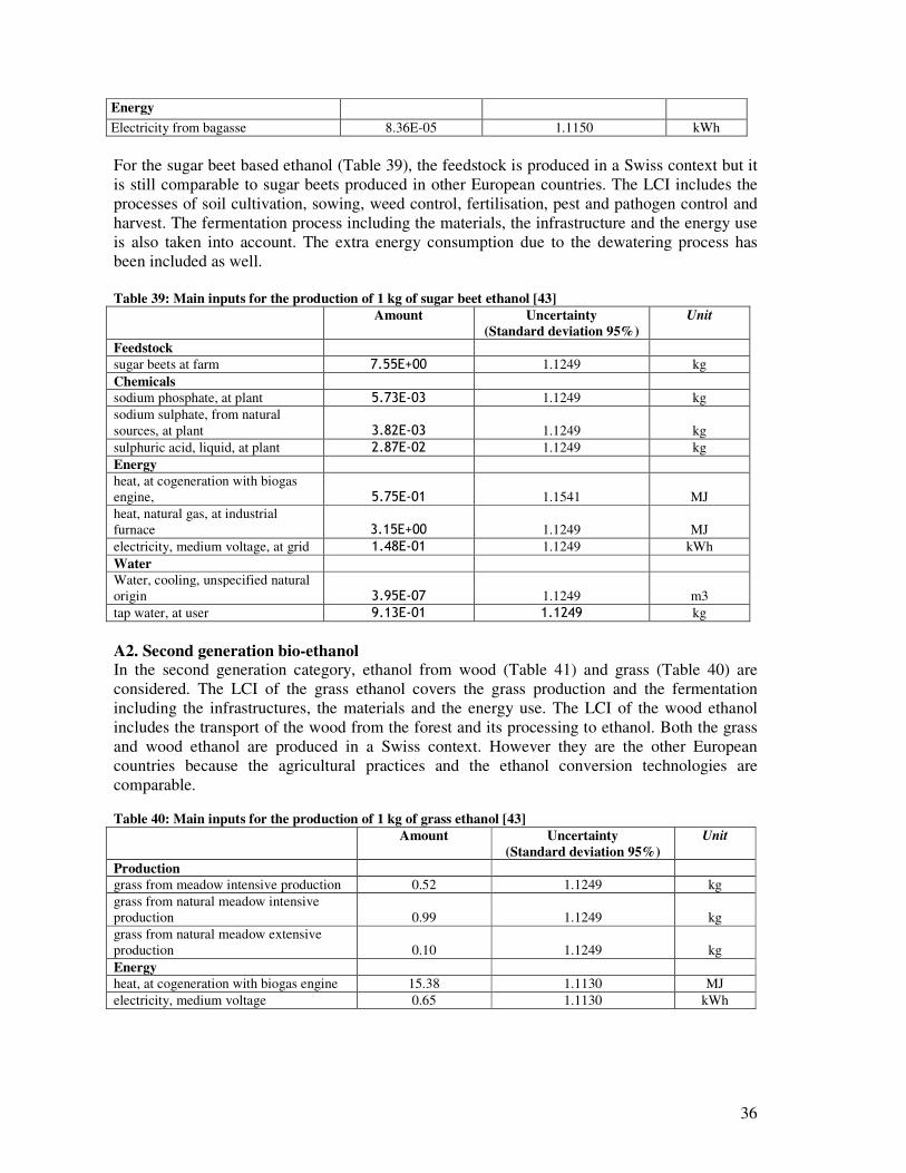
36

Energy Electricity from bagasse 8.36E-05 1.1150 kWh

For the sugar beet based ethanol (Table 39), the feedstock is produced in a Swiss context but it

is still comparable to sugar beets produced in other European countries. The LCI includes the

processes of soil cultivation, sowing, weed control, fertilisation, pest and pathogen control and

harvest. The fermentation process including the materials, the infrastructure and the energy use

is also taken into account. The extra energy consumption due to the dewatering process has

been included as well.

Table 39: Main inputs for the production of 1 kg of sugar beet ethanol [43]

Amount Uncertainty


Unit

Feedstock

sugar beets at farm 7.55E+00 1.1249 kg

Chemicals

sodium phosphate, at plant 5.73E-03 1.1249 kg

sodium sulphate, from natural

sources, at plant 3.82E-03 1.1249 kg

sulphuric acid, liquid, at plant 2.87E-02 1.1249 kg

Energy

heat, at cogeneration with biogas

engine, 5.75E-01 1.1541 MJ

heat, natural gas, at industrial

furnace 3.15E+00 1.1249 MJ

electricity, medium voltage, at grid 1.48E-01 1.1249 kWh

Water

Water, cooling, unspecified natural

origin 3.95E-07 1.1249 m3

tap water, at user 9.13E-01 1.1249 kg

A2. Second generation bio-ethanol In the second generation category, ethanol from wood (Table 41) and grass (Table 40) are

considered. The LCI of the grass ethanol covers the grass production and the fermentation

including the infrastructures, the materials and the energy use. The LCI of the wood ethanol

includes the transport of the wood from the forest and its processing to ethanol. Both the grass

and wood ethanol are produced in a Swiss context. However they are the other European

countries because the agricultural practices and the ethanol conversion technologies are

comparable.

Table 40: Main inputs for the production of 1 kg of grass ethanol [43]

Amount Uncertainty


Unit

Production

grass from meadow intensive production 0.52 1.1249 kg

grass from natural meadow intensive

production 0.99 1.1249 kg

grass from natural meadow extensive

production 0.10 1.1249 kg

Energy

heat, at cogeneration with biogas engine 15.38 1.1130 MJ

electricity, medium voltage 0.65 1.1130 kWh

37

Table 41: Main inputs for the production of 1 kg of wood ethanol [43]

Amount Uncertainty

(Standard deviation 95%) Unit

Feedstock wood chips, hardwood, at forest 1.61E-02 1.2229 m3

Chemicals

maize starch, at plant 2.64E-02 1.2229 kg

Chemicals sulphuric acid, liquid, at plant 8.26E-02 1.2229 kg

ammonia, liquid, at regional storehouse 6.59E-02 1.2229 kg

magnesium sulphate, at plant 5.43E-04 1.2229 kg

calcium chloride, CaCl2, at regional

storage 1.20E-03 1.2229 kg

chlorine, liquid, production mix, at plant 5.81E-06 1.3241 kg

sodium chloride, powder, at plant 7.26E-05 1.3241 kg

ammonium sulphate, as Nitrogen, at

regional storehouse 1.18E-03 1.2229 kg

diammonium phosphate, as N, at regional

storehouse 1.67E-03 1.2229 kg

chemicals organic, at plant 2.39E-04 1.2229 kg

lubricating oil, at plant 5.81E-05 1.3241 kg

urea, as Nitrogen, at regional storehouse 4.74E-04 1.3241 kg

Water

tap water, at user 8.03E+00 1.2229 kg

water, decarbonised, at plant 1.39E-02 1.3241 kg

B. Methanol (Fischer-Tropsch) Bio-methanol can be produced from ‘wood synthetic gas’ (Table 42) which is a gasified wood.

The production process is a full-methanol steam reforming. The LCI of the methanol (Table 43)

includes the production of synthetic gas from wood chips and the production of methanol

derived from the synthetic gas. The extra hydrogen produced during the steam reforming is

burned in the furnace of the plant. The processing energy as well as the use of catalysts is taken

into account.

Table 42: Main input for the production of 1 kg of synthetic gas from wood [43].

Amount Uncertainty


Units

Energy


Wood

wood chips, mixed at forest 1.71 E-03 1.3120 m3

wood chips, mixed, from industry, 5.88 E-04 1.3120 m3

waste wood chips, mixed, from industry, 3.74 E-04 1.3120 m3

Water

tap water 0.14 E00 1.3960 kg

washing agents

zeolite 20.80 E-04 1.3960 kg

Chemicals

sodium hydroxide, 50% in water 82.80 E-05 1.3279 kg


38

Table 43: Main input for the production of 1 kg of methanol from synthetic gas [43].

Amount Uncertainty


Unit

Chemicals

aluminium oxide 2.40 E-04 2.1586 kg

copper oxide 9.00 E-05 2.1586 kg

Production

synthetic gas 7.13 E00 1.5226 Nm3

Energy

electricity, medium voltage 0.28 E00 1.6512 kWh

Water

water, deionised, 0.85 E00 1.5319 kg

C. Biodiesel

C1. First generation biodiesel Two first generation biodiesels will be considered in the CLEVER project:

• Rape methyl ester (RME) which is the most developed biodiesel in Europe (2000

kilotons in 2004 [43])

• Soybean methyl ester (SME) produced in the US and imported to Europe.

The inventory of RME (Table 45) includes the processes of soil cultivation, sowing, weed

control, fertilization, pest and pathogen control, harvest and drying of the grains, transport, oil

extraction (Table 44) and the esterification processes. The machine infrastructure and sheds for

machine sheltering are also included.

Table 44: Main input for the extraction of 1 kg of rape oil [43].

Amount Uncertainty


Unit

Production

rape seed 1.91 E00 1.0722 kg

Chemicals

hexane 20.92 E-04 1.0913 kg

phosphoric acid, 85% in water 6.76 E-04 1.0913 kg

Energy



Table 45: Main inputs for the production of 1 kg of rape methyl ester [43].

Amount Uncertainty (Standard deviation 95%)

Unit

Production

rape oil 0.89 E00 1.2090 kg

Chemicals

phosphoric acid, 85% in water 39.98 E-04 1.0913 kg

potassium hydroxide 98.66 E-04 1.0913 kg

methanol 986.92 E-04 1.0722 kg

Energy


heat, natural gas, at industrial furnace 8025.42 E-04 1.0722 MJ

Water

tap water 237.38 E-04 1.5642 kg

For the SME, the cultivation of soybeans in the US, the use of machines, fertilizers and

pesticides, as well as the transport to the oil mill, the oil extraction (Table 46) and the

39

esterification (Table 47) are included in the LCI. The transport of the final product from the US

to Europe has been taken into account as well.

Table 46: Main inputs for the extraction of 1 kg of soybean oil [43].

Amount Uncertainty


Unit

Production

soybeans 1.83 E00 1.1130 kg

Water

tap water 0.16 E00 1.1668 kg

Chemicals

hexane 39.24 E-04 1.1668 kg

phosphoric acid, industrial grade 3.09 E-04 1.0752 kg

Energy


heat, at hard coal industrial furnace 0.15 E00 1.1668 MJ

heat, light fuel oil, at industrial furnace 565.96 E-04 1.1668 MJ


Table 47: Main inputs for the production of 1 kg of soybean methyl ester [43]

Amount Uncertainty


Unit

Production

soybean oil 0.95 E00 1.2093 kg

Chemicals

hydrochloric acid, 30% in water 42.36 E-04 1.0913 kg

phosphoric acid,, 85% water 104.53 E-04 1.0913 kg

methanol 1045.64 E-04 1.0722 kg

Energy


heat, at hard coal industrial furnace 960.86 E-04 1.0722 MJ

heat, light fuel oil, at industrial furnace 374.13 E-04 1.0722 MJ

heat, natural gas, at industrial furnace 7167.91 E-04 1.0722 MJ

Water

tap water 251.50 E-04 1.5642 kg

C2. Second generation biodiesel The most developed second generation biodiesel in Europe is the waste cooking oil methyl ester

(Table 48). Waste vegetable oil is collected and treated in dedicated plants in which all the

impurities and water are removed. At the end of the process a treated vegetable oil consisting of

93.7% triglycerides and 6.7 % fatty acid methyl ester is obtained. The process refers to the

catalyzed estherification of free fatty acids. The LCI covers the collection, the treatment, the

conditioning, the storage and the treatment of the effluents.

Table 48: Main input for the production of 1 kg of waste cooking oil methyl ester [43].

Amount Uncertainty


Unit

Energy

electricity, medium voltage 508.0 4E-4 1.6211 kWh


Chemicals

methanol 2.69 E-02 1.5955 kg

glycerin, from vegetable oil, 10.56 E-02 1.5955 kg


40

D. Biogas Biogases are produced from miscellaneous substrates. The major production routes are

fermentation of bio-waste, sewage sludge, whey, grass, liquid manure and co-fermentation of

liquid manure and bio-waste. In all the cited biogases, only biogas from bio-waste is further

upgraded to natural gas quality which can be used as a transportation fuel for natural gas

vehicles [26], the other biogases are being used for heat and electricity co-generation. For the

CLEVER project, biogas from bio-waste fermentation (Table 49) will be considered. Bio-waste

contains biogenous household waste, garden waste and food waste.

The LCI covers the pre-treatment (including the disposal of contaminants), the digestion and

post-composting of digested matter. The emissions to soil due to the use of presswater and

digested matter as a fertilizer in agriculture are taken into account. The spreading of the

fertilizer as well as the transport from the bio-waste plant to farms is also taken into account.

The electricity consumption during the biogas upgrading (raw gas compression, H2S removal,

gas conditioning and methane enrichment of biogas) is included in the LCI as well. 1.5 Nm3 of

raw biogas is needed to produce 1 Nm3 of methane with a purity of 96% and 0.5 kWh of

electricity is used for this purification.

Table 49: Energy consumption for the production of 1Nm

3 of biogas from biowaste [43].

Amount Uncertainty (Standard deviation 95%)

Unit

Energy

heat, natural gas, at boiler 1.08 E00 1.2335 MJ

electricity, low voltage 7.3 E-02 1.2335 kWh

IV.12. Battery Ellectric Vehicles, Fuel Cell Electric Vehicle and Hybrid Electric Vehicles

LCI data of batteries were collected from the SUBAT project [44] in which ETEC-VUB was

involved. The LCI covers both Hybrid Electric Vehicles (HEV) and Battery Electric Vehicles

(BEV). The material breakdown as well as the assembly energy of the different battery

technologies is included. Manufacturing data of supercapacitors were provided by the Maxwell

company which is a partner of the HyHEELS [45] project in which ETEC-VUB is involved as

well.

For the specific cases of BEV and FCEV, the Tesla Roadster and the Honda FCX Clarity have

been respectively chosen. The ratio between the life time driven distance (230500 km) and the

cycle life of the lithium-ion battery (100000 miles or 160934.4 km) [46] has been used to

calculate the number of the needed batteries for the BEV. On the basis of this calculation, 1.43

batteries are used during the lifetime of the vehicle. The weight of the battery is approximately

408 kg (900 pounds) [46]. In the case of the FCEV, a lifespan of 5000 hours (typical value for

fuel cells in automotive application) has been considered for the fuel cell. As a consequence,

only one fuel cell stack is considered for the FCEV.

Inventory data of parts and components (body shell, tires, lead acid batteries…) which are

common to all the vehicle technologies are collected and adapted as a parameter to each vehicle

according to its specifications. Data for specific parts of specific vehicle technologies such as

Nickel-Metal hydride (NIMH) batteries, Lithium-ion batteries (, fuel cells, hydrogen tanks…etc

are gathered separately for the corresponding vehicles and included in the model. For each

vehicle, common parts and specific parts are combined with respect to their weight percentages

to model the manufacturing step.

For alternative vehicles such as BEV and FCEV, the LCI of the Golf A4 has been used to

model only the body shell. Inventory data of specific parts of the cars such as hydrogen tanks

and fuel cells (see paragraph IV.2) have been gathered from [27].

41

IV.13. Maintenance

As for the manufacturing phase, a theoretical maintenance (Table 50) process has been

modeled. It will contain oil (Table 53) consumption, tires (Table 52), batteries for hybrid or

electric vehicles and washing water during the lifespan of the vehicle. The theoretical

maintenance process corresponds to a Golf A4 diesel which weighs 1181 kg and is used to

fulfill the functional unit (230500 km). The calculations are based on the assumptions of the

IMPRO-car project [47] and the Life Cycle Inventory for the Golf A4 [48]. The equation (1)

used for the manufacturing phase will be used to extend that maintenance process to the other

vehicles.

Close to the spare parts, the emitted particles from the abrasion of tire wear and break wear

(Table 51) will also be taken into account [49]

Table 50: Theoretical maintenance process. [47, 48].

Amount (230500 km)

tires 165.96 kg

lead-acid batteries 64.54 kg

oil 67.61 kg

washing water 12.29 m3

Table 51: Non-exhaust emissions of passenger vehicle [49]

PM 10-PM2.5 PM2.5

g/km g/km

tire wear emitted particles 0.0037 0.0027

brake wear emitted particles 0.0043 0.0031

Table 52: Material breakdown of a tire [47, 48]

Materials Weight%

rubber 48.00

carbon black 22.00

steel 15.00

textile 5.00

zinc oxide 1.00

Sulphur 1.00

additives (xylene, benzene, phenol) 8.00

Table 53: Main inputs for the production of 1 kg of lubricant oil [38].

Amount Uncertainty (Standard

deviation 95%)

Unit

Oil

diesel 1.33 1.20 kg

Energy

electricity, medium voltage 0.33 1.90 kWh

heat, natural gas, at industrial furnace 2.00 1.90 MJ

IV.14. End-of-life

End-of-life data have been provided by RDC-Environment, which has performed a study on

end-of-life vehicles for the Flemish public waste management organization (OVAM). The

global recycling rate of vehicles and consumption of resources during the recycling process

have been included, as well as the range of recycling rates per type of material (Table 54). The

efficiency of recycling processes and the real capacity of recycling plants were taken into

42

account as well. As for the manufacturing and the maintenance phases, the end-of-life phase of

the body shell has been modelled as a parameter which will be adapted to all the vehicles

according to their weight. An energy consumption of 66kWh/ton [50] is considered for the

shredding and the further separation processes. As batteries in end-of-life vehicles should be

removed and treated separately during the depollution step of end-life vehicles, their treatment

has been assessed separately. Different recycling processes have been considered according to

the battery technology: Hydrometalurgical process for lithium ion technology (Table 55),

pyrometalurgical for NiMH and NiCd technologies (Table 56 and Table 58)and the Campine

process for Lead acid technology(Table 57) [51]. These processes are modelled within this

study on an input/output basis with respect to the energy and chemical consumption at the input

side and to the recycling efficiency per type of material at the output side. The recycling rates

per type of materials of EoL vehicles are the ones from the OVAM/RDC study (Table 54).

Non-recyclable chemicals are landfilled since most of them are not accepted in the incineration

process. For supercapacitors, the aluminum, the ABS, the copper and the steel are considered to

be recyclable. Since we have no energy consumption for the recycling of supercapacitors, the

battery recycling process with the highest energy consumption has been considered for it (4.72

MJ/Kg).

Table 54: Recovery rates of end-of -life vehicle materials [10].

Material

Average recycling rate

(%)

Average energetic valorisation rate

(%)

Total recovery rate

(%)

ferro-metals 99.82 0.00 99.82

aluminium 93.20 0.00 93.20

copper 88.53 0.00 88.53

zinc 93.49 0.00 93.49

lead 91.43 0.00 91.43

polypropylene 51.99 2.47 54.47

polyethylene 51.99 2.47 54.47

PMMA 3.00 29.49 32.49

ABS 49.27 4.95 54.21

PET 0.73 35.53 36.26

EPP 2.93 0.01 2.94

PP-EPDM 5.55 2.47 8.02

polyurethane 5.58 1.03 6.61

rubber 3.47 28.56 32.03

textile 6.19 2.10 8.29

Table 55: Hydrometallurgical recycling of Lithium Ion battery [51]

Amount Unit

Inputs

EoL battey 1000 kg

reagent 25 kg

electricity 140 kWh

industrial water 0.72 m3

sulphuric acid 126 L

lime 116 kg

Recycling efficiency

cobalt 1.00

lithium 1.00

iron and steel 0.75

non ferrous metals 0.94

43

Table 56: Pyrometallurgical recycling of NiMH battery [51]

Amount Unit

Inputs

EoL battey 1000 kg

active carbon 1.67 kg

electricity 310 kWh

natural gas and propane 94.7 kg

process water 240 l

Recyccling efficiency

nickel-cobalt-iron 0.73

Table 57: Campine Lead acid battery recycling [51]

Amount Unit

Inputs

EoL battery 1000 kg

limestone 5.8 kg

iron scrap 4.0 kg

sodium hydroxide 350 kg

sodium nitrate 0.4 kg

sulphur 0.9 kg

iron chloride 0.9 kg

slag 150 kg

electricity 35.2 kg

natural gas 16.2 kg

coke 20.0 kg

process water 770 kg

Recycling efficiency

lead 1.00

sulphuric acid for reuse 0.44

Table 58: Pyrometallurgical recycling of NiCd battery [51]

Amount Unit Inputs EoL battey 1000 kg active carbon 1.67 kg electricity 1545 kWh propane/butane 170.6 kg process water 240 kg Recycling efficiency cadmium 0.90 nickel-iron 0.95

IV.15. Tank to Wheel (TTW) data

The Ecoscore database is the reference database for direct or Tank to-Wheel (TTW) emission

data for the CLEVER project. It contains fuel/energy consumption and emission data resulting

from the vehicle’s homologation procedure. The average CO2 emissions (g/km) as well as the

HC, SO2, NOx, CO, PM, CH4, N2O emissions (g/km) for each specific vehicle are contained in

the Ecoscore database. The consumption of liquid fuels is expressed in l/100 km, of gases in

m3/100 km and of electric energy in kWh/km. As the emissions are measured with the New

European Driving Cycle (NEDC) combining urban and extra-urban driving cycles, only

average emissions and fuel consumption are available in the Ecoscore database. Therefore

splitting up direct emissions into urban and extra-urban conditions is not possible. However, the

CLEVER LCA model is developed to assess the environmental impact of both urban and extra-

urban driving when the needed data will be available. The testing conditions under NEDC do

not include the additional fuel consumption of the cooling and the heating devices (Chasserot

M. 2007). The considered weight for the vehicle is

coolant, oils, fuel, spare wheels, tools and the driver (75 kg).(Directive 92/21/EEC

The Ecoscore database contains different vehicle technologies (petrol, diesel, battery electric,

hybrid electric, and flexi-fuel) and different vehicle

The modelling parameters of the life cycle of the different vehicles are extracted from the

Ecoscore database. A data analysis was performed to extract these parameters from the raw data

available in the Ecoscore database. Since the

modelling parameters are not fixed values but ranges. In the model, all the possible variations

of these parameters are taken into account, resulting in a variation of the considered impacts.

When including the frequencies of these values, one can match a triangular or uniform

distribution with the real distribution of the values.

this approach for a Euro 4 family car using petrol.

There are strong correlations between fuel consumption and vehicle weight, carbon dioxide and

sulphur dioxide. These parameters can be described as a linear function of fuel consumption,

multiplied with an ‘error’ distribution, expressing the difference between the linear equation

and the real distribution of the parameter. For the other emissions (HC, NOx, CO, PM,

and N2O), no satisfying correlation with fuel consumption was found. These emissions are

modelled as a triangular or a uniform distribution, matching the reality as closely as possible.

The chosen distributions have an important impact on the overall

conclusions of the data analysis are therefore interesting to discuss.

Fuel consumption, weight, CO2 and SO

other side, the Euro standard does not influence these parameters. Impacts o

and well-to-tank emissions do not change by introducing newer Euro standards. Tank

(TTW) emissions of CO2 and SO2 will also not change by introducing newer euro standards. On

the other hand it is noticeable that the Euro standard i

emissions. The higher the Euro standard, the lower HC, NO

are.

Figure 4: Range of the fuel consumption of the family petrol Euro 4 car


M. 2007). The considered weight for the vehicle is the ‘in running order’ mass including

nt, oils, fuel, spare wheels, tools and the driver (75 kg).(Directive 92/21/EEC) The Ecoscore database contains different vehicle technologies (petrol, diesel, battery electric,

fuel) and different vehicle segment (see chapter I) of the Belgian fleet.



available in the Ecoscore database. Since the Belgian fleet includes a large variety of cars, the



ng the frequencies of these values, one can match a triangular or uniform

distribution with the real distribution of the values. Figure 4 and Figure 5 give an example of

this approach for a Euro 4 family car using petrol.


hese parameters can be described as a linear function of fuel consumption,


and the real distribution of the parameter. For the other emissions (HC, NOx, CO, PM,



The chosen distributions have an important impact on the overall result, preliminary

conclusions of the data analysis are therefore interesting to discuss.

and SO2 are highly dependent of the chosen segment. On the

other side, the Euro standard does not influence these parameters. Impacts of manufacturing

tank emissions do not change by introducing newer Euro standards. Tank

will also not change by introducing newer euro standards. On

the other hand it is noticeable that the Euro standard influences highly the other regulated TTW

emissions. The higher the Euro standard, the lower HC, NOx, CO, PM, CH4 and N2O emissions

: Range of the fuel consumption of the family petrol Euro 4 car


the ‘in running order’ mass including

The Ecoscore database contains different vehicle technologies (petrol, diesel, battery electric,

of the Belgian fleet.



Belgian fleet includes a large variety of cars, the



ng the frequencies of these values, one can match a triangular or uniform

give an example of


hese parameters can be described as a linear function of fuel consumption,


and the real distribution of the parameter. For the other emissions (HC, NOx, CO, PM, CH4



result, preliminary

are highly dependent of the chosen segment. On the

f manufacturing

tank emissions do not change by introducing newer Euro standards. Tank-to-wheel

will also not change by introducing newer euro standards. On

nfluences highly the other regulated TTW

O emissions

Figure 5: Distribution of the fuel consumption of the family petrol Euro 4 car

As heavy metal emissions are not available in the Ecoscore database, emission factors in terms

of mg of substance per kg of burned fuel are gathered from the EMEP

inventory guidebook [49] for petrol and diesel cars (

Next to the Ecoscore database, some bio

Ecoinvent v2.0 have been collected as well. These emissions correspond to a range of vehicles

with a weight between 1300 and 1500 kg [

family car’ category according to the classification made in the CLEVER project. The

phases of E5 (petrol with 5% ethanol), methane from biogas, diesel with 5% RME, methanol,

petrol with 4% ETBE and petrol with 15% ETBE are included. The emission measurements

have been done with the New European Driving Cycle.

Furthermore, bio-fuel TTW emissions of the Volvo

C4 have been provided by the BIOSES project (

Table 59: heavy metal emissions of passenger car [

mg/kg burned petrol

cadmium 0.01

copper 1.70

chromium 0.05

nickel 0.07

selenium 0.01

zinc 1.00

lead 2.00E

mercury 7.00E

chromium IV 1.00E

Note: 0.2% of the emitted chrome is emitted as Chromium (IV

: Distribution of the fuel consumption of the family petrol Euro 4 car


of mg of substance per kg of burned fuel are gathered from the EMEP/CORINAIR emission

] for petrol and diesel cars (Table 59).

Next to the Ecoscore database, some bio-fuels’ Tank-to-Wheel data (Table 60) available in

have been collected as well. These emissions correspond to a range of vehicles

with a weight between 1300 and 1500 kg [52]. This range of vehicles corresponds to the ‘small

family car’ category according to the classification made in the CLEVER project. The



have been done with the New European Driving Cycle.

TW emissions of the Volvo F50, the Saab 9.5 BioPower and the Citroen

C4 have been provided by the BIOSES project (Table 61, Table 62and Table 63)

missions of passenger car [49]

mg/kg burned petrol mg/kg burned diesel

0.01

1.70

0.05

0.07

0.01

1.00

2.00E-03 1.10E-07

7.00E-05 2.00E-05

1.00E-04 1.00E-04

Note: 0.2% of the emitted chrome is emitted as Chromium (IV)


/CORINAIR emission

) available in

have been collected as well. These emissions correspond to a range of vehicles

]. This range of vehicles corresponds to the ‘small

family car’ category according to the classification made in the CLEVER project. The use



and the Citroen

46

Table 60: TTW emissions of bio-fuel vehicles [43].

Biomethane

(g/km)

E5

(g/km)

M100

(g/km)

B5

(g/km)

Petrol/ETBE15

(g/km)

Petrol/ETBE4

(g/km)

CO fossil 0.00E00 8.75E-04 0.00E00 6.09E-04 7.22E-04 7.47E-04

CO bio 4.46E-01 2.95E-02 9.31E-01 2.86E-02 3.31E-02 8.63E-03

CO2 fossil 0.00E00 189.00E00 0.00E00 166.00E00 177.00E00 183.00E00

CO2 bio 172.00E00 6.36E00 177.00E00 7.80E00 8.09E00 2.12E00

CH4 fossil 0.00E00 4.79E-03 0.00E00 3.37E-03 5.26E-03 5.44E-03

CH4 bio 4.51E-02 1.61E-04 1.44E-03 1.58E-04 2.41E-04 6.29E-05

NOx 2.06E-02 5.84E-05 3.84E-02 5.05E-01 3.56E-02 3.56E-02

PM 6.67E-04 1.98E-03 0.00E00 3.16E-02 1.00E-01 1.00E-01

N2O 8.66E-04 2.57E-03 2.60E-03 5.58E-03 1.33E-03 1.33E-03

SO2 8.95E-04 5.99E-03 0.00E00 5.25E-03 5.13E-03 5.04E-03

NMVOC 1.05E-02 5.84E-02 5.18E-02 1.29E-01 9.33E-02 9.33E-02

Benzene 7.62E-04 1.88E-03 2.74E-03 1.80E-03 8.89E-03 8.89E-03

Toluene 5.25E-03 8.71E-03 5.56E-03 4.15E-04 7.68E-03 7.68E-03

Xylene 5.39E-03 9.31E-03 5.28E-04 1.04E-03 7.68E-03 7.68E-03

Table 61: TTW emissions of the Citroen C4 using different blends of diesel [53].

Fuel consumption (l/100 km)

CO2 (g/km)

CO (g/km)

NOx (g/km)

HC (g/km)

diesel 5.79 152.4 3.4E-2 0.64 1.3 E-2

B5 6.03 159.1 2.8E-2 0.61 1.0 E-2

B10 5.94 156.0 2.3 E-2 0.58 1.0 E-2

B30 5.85 151.3 1.4 E-2 0.63 0.9 E-2

B100 6.07 149.7 1.2 E-2 0.71 1.6 E-2

Table 62: TTW emissioons of the Saab 9.5 BioPower using different blends of petrol [53]

Fuel consumption

(l/100 km)

CO2

(g/km)

CO

(g/km)

NOx

(g/km)

HC

(g/km)

diesel 10.49 247.74 0.26 3.66E-03 5.36E-03

E5 10.43 240.78 0.31 2.85E-03 5.40E-03

E10 10.67 239.71 0.18 2.92E-03 4.48E-03

E30 10.44 222.11 0.08 2.84E-03 2.27E-03

E85 13.30 212.97 0.05 2.61E-03 2.15E-03

Table 63: TTW emissions of the Volvo F50 using different blends of petrol [53]

Fuel consumption

(l/100 km)

CO2

(g/km)

CO

(g/km)

NOx

(g/km)

HC

(g/km)

Euro 95 7.40 175.63 0.21 17,33E-3 0.76E-3

E5 7.63 176.31 0.19 16.52E-3 0.69E-3

E10 7.93 178.07 0.21 20.02E-3 0.87E-3

E20 8.56 181.71 0.25 18.73E-3 0.99E-3

E85 12.16 192.90 0.15 18.73E-3 1.05E-3

Additionally, tailpipe emissions (Table 64) of two hydrogen vehicles have been collected from

[54, 55]. It is important to mention that contrarily to the other vehicle technologies, the

considered FCEV vehicle in this study is not yet homologated in Europe. Thus, an NEDC based

fuel consumption is not available for this vehicle. So, an US EPA (Environmental Protection

Agency) combined cycle based fuel economy of 60 miles (96.56 km) per kg has been

considered for the FCEV (Honda 2010). The Honda FCX Clarity has a driving range of 240

miles (386.23 km).

47

Table 64: TTW emissions of 2 prototype hydrogen vehicles [54], [55]

Air conditioning systems

According to [56], the use of an air conditioning system increases the vehicle’s fuel

consumption by 17.8 %, but this could vary according to the technology, the meteorological

conditions and the driving style. For example the extra consumption due to the air conditioning

ranges from 12 to 43% in an urban driving context according to the type of engine and the

driving behavior. Additionally, the extra consumption due to the weight of the air conditioning

system is about 8.2%.

IV.16 Conclusion

The LCI step of the CLEVER project has been performed thanks to a special data gathering

strategy. A list of all the relevant data sources and projects has been made during a detailed

literature review. Priority has been given to specific Belgian and European data. The Ecoinvent

v2.0 and Ecoscore databases have been the main data sources. Raw material production,

manufacturing, transport, fuel, energy, maintenance and Well-to-Wheel data are collected for

conventional and alternative vehicles. However, some adaptations have been made to avoid

repetition and to solve the problem with lack of data. Thus, for the manufacturing phase

complete LCI data of the VW Golf have been used to model a theoretical car which is used as a

parameter to model the other cars proportionately to their weight. For the emission control

technologies, only LCI data of a sedan catalytic converter are obtained. It is also important to

note that average Tank-to-Wheel data are considered instead of urban and extra-urban data

since the direct emissions come from the New European Driving Cycle.

Finally, the gathering of direct emissions of bio-fuel cars has been completed by the emission

measurement campaign which has been performed by the BIOSES project.

V. Life Cycle Impact Assessment After the completion of the LCI, the different elementary flows that are linked to a product

system need to be converted into environmental indicators. These indicators allow quantifying

and comparing the potential environmental impacts of the different product systems. This step

of the LCA is called Life Cycle Impact Assessment (LCIA). The LCIA has mandatory and

optional elements. The mandatory elements include the selection of impact categories, the

assignment of the elementary flows to the categories (classification) and the attribution of

factors to each elementary flow according to its relative contribution to the category

(Characterisation). The optional elements are the calculation of the magnitude of an impact

category relative to reference information (normalization) and the grouping of the different

impact indicators into a single score (weighting).[57]. However, weighting shall not be used for

comparative LCA studies intended to be disclosed to the public [58].

As required by [58], LCIA category indicators and characterisation models based on

international agreement should be used. In this perspective, the European commission via the

Vehicle Technology storage Fuel

[kg H2/km]

NOx

[g/km]

CO

[g/km]

CO2

[g/km]

NMHC

[g/km]

Ford P2000 H2-ICEV 1,5 kg at 248

bar 4.40E-03 4.60E-01 5.10E-03 8.70E-01 4.70E-03

Honda FCX

Clarity FCEV

3.92 kg at

345 bar 1.04E-02 0.00E+00 0.00E+00

0.00E+0

0

0.00E+0

0

48

Joint Research Centre (JRC) has initiated the International Reference Life Cycle Data System

(ILCD) in order to ‘provide governments and businesses with a basis for assuring quality and

consistency of life cycle data, methods and assessments’ [59]. In the framework of the ILCD activities,

an analysis of the existing LCIA methods has been performed [60]. In this analysis, the main existing

methodologies are described regarding the documentation, the general principals, the consistency across

a list of predefined impact categories and the interesting innovative aspects [60]. Finally, a list of

preselected LCIA methods has been produced (Table 65). These preselected LCIA methods will be

assessed in details by the ILCD team and a final list is expected for 2011.

Table 65: Pre-selection of characterisation models for further analysis [60]

49

In this study, it has been decided to use only LCIA methods preselected in the framework

of the ILCD activities and which are relevant for the specific context of automotive LCA.

The selected methods are:

• IPCC 2007 [61]

• Air acidification [62]

• Eutrophication [62]

• Mineral extraction [63]

• renewable and non renewable energy demand

• Respiratory effects (inorganics) [64]

As it can be noticed in Table 66 to Table 72, the most important and relevant elementary flows

are considered in the selected impact calculation methods. Endpoint methods, excepted

respiratory inorganics, have been used for all the selected impact categories.

For the specific cases of renewable and non renewable energy demand, the calculation method

has been developed by RDC-ENVIRONMENT with inputs from themselves and from the

Swiss Agency for the Environment, Forests and Landscape (BUWAL). The energy demand

(Table 69 and Table 70) includes all the types of primary energy involved in a product system.

It also includes the heating value of products, resources and materials.

The respiratory inorganics impact on human health (

Table 71) is particularly interesting in this study because it includes particulates, carbon

monoxide and nitrogen and sulphur based emissions. These emissions are among the pollutants

allowing clear differenction between vehicle technologies and fuels.

The IPCC 2007 (100a) method has been extended to biogenic CO2 and the CO2 uptake from the

air during the synthesis of the organic matter. A negative factor is attributed to the CO2 uptake.

The air acidification (Table 67) and eutrophication (Table 68) calculation expressed

respectively in kg SO2eq/kg and kg PO4eq/kg are from the CML 2001 methodology [62]. It

includes mainly nitrogen, sulphur and phosphorus based emissions. These two methods allow

performing a comprehensive assessment of the effect of the fertilizers for biofuels on one hand

and assessing the impact of the use of products and resources containing sulphur (e.g. crude

oil), phosphorus or nitrogen.

The mineral extraction damage (Table 72) expressed in MJ surplus/kg allows assessing the

additional energy requirement for further mining of the mineral resources in the future due to

the lower resource concentration. This method is particularly interesting for the manufacturing

phase of vehicles in general and the manufacturing of specific components ( battery, fuel cell,

hydrogen tank…) in particular.

Table 66: IPCC 2007 (100a) including biogenic CO2 and CO2 uptake from the air [61]

Elementary flows

Characterisation factor

(kg CO2 eq/kg)

CFC 12 (CCl2F2) 10900 CFC 113 (CFCl2CFCl2) 6130 HFC 23 (CHF3) 14800 HCFC 21 (CHCl2F) 210 CFC 11 (CFCl3) 4750 Chloroform (CHCl3) 756

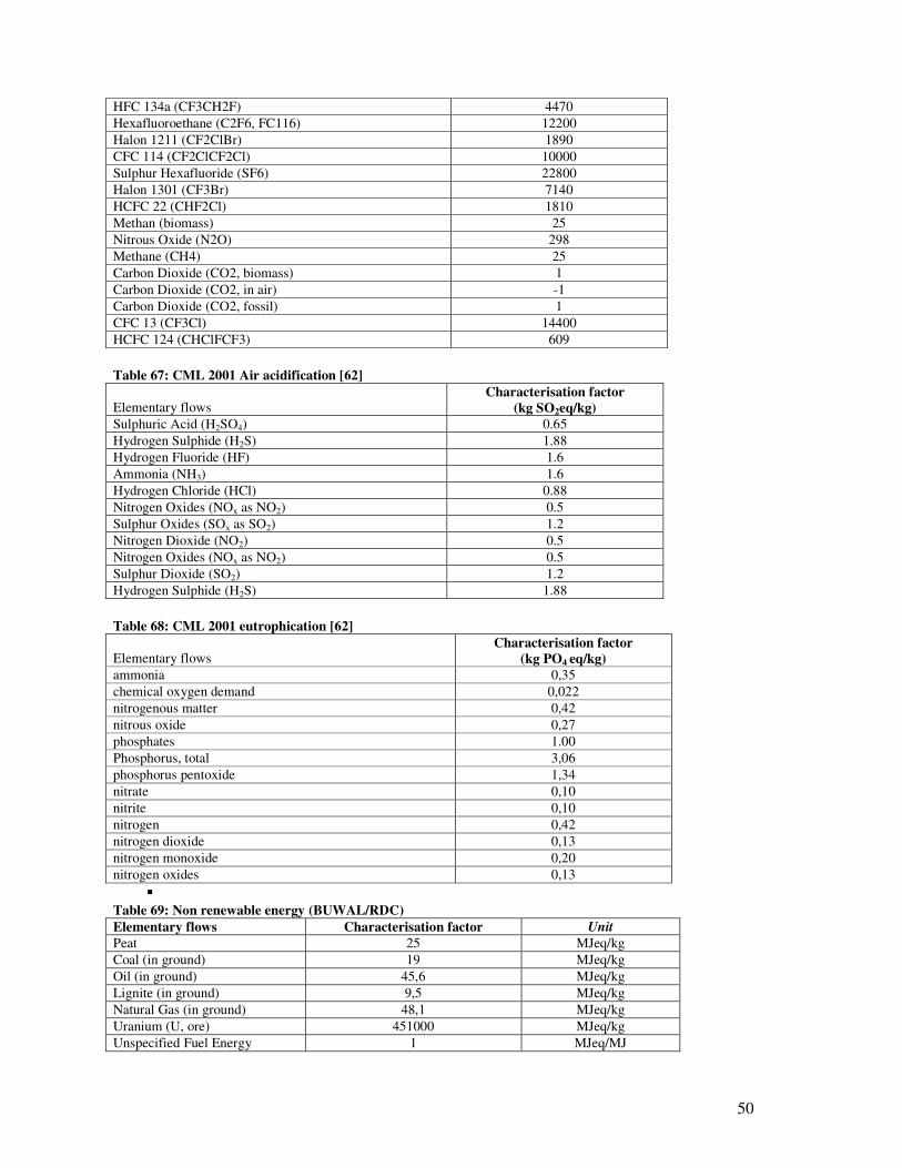
50

HFC 134a (CF3CH2F) 4470 Hexafluoroethane (C2F6, FC116) 12200 Halon 1211 (CF2ClBr) 1890 CFC 114 (CF2ClCF2Cl) 10000 Sulphur Hexafluoride (SF6) 22800 Halon 1301 (CF3Br) 7140 HCFC 22 (CHF2Cl) 1810 Methan (biomass) 25 Nitrous Oxide (N2O) 298 Methane (CH4) 25 Carbon Dioxide (CO2, biomass) 1 Carbon Dioxide (CO2, in air) -1 Carbon Dioxide (CO2, fossil) 1 CFC 13 (CF3Cl) 14400 HCFC 124 (CHClFCF3) 609

Table 67: CML 2001 Air acidification [62]

Elementary flows Characterisation factor

(kg SO2eq/kg)

Sulphuric Acid (H2SO4) 0.65 Hydrogen Sulphide (H2S) 1.88 Hydrogen Fluoride (HF) 1.6 Ammonia (NH3) 1.6 Hydrogen Chloride (HCl) 0.88 Nitrogen Oxides (NOx as NO2) 0.5 Sulphur Oxides (SOx as SO2) 1.2 Nitrogen Dioxide (NO2) 0.5 Nitrogen Oxides (NOx as NO2) 0.5 Sulphur Dioxide (SO2) 1.2 Hydrogen Sulphide (H2S) 1.88

Table 68: CML 2001 eutrophication [62]

Elementary flows Characterisation factor

(kg PO4 eq/kg)

ammonia 0,35

chemical oxygen demand 0,022

nitrogenous matter 0,42

nitrous oxide 0,27

phosphates 1.00

Phosphorus, total 3,06

phosphorus pentoxide 1,34

nitrate 0,10

nitrite 0,10

nitrogen 0,42

nitrogen dioxide 0,13

nitrogen monoxide 0,20

nitrogen oxides 0,13

�

Table 69: Non renewable energy (BUWAL/RDC)

Elementary flows Characterisation factor Unit

Peat 25 MJeq/kg

Coal (in ground) 19 MJeq/kg

Oil (in ground) 45,6 MJeq/kg

Lignite (in ground) 9,5 MJeq/kg

Natural Gas (in ground) 48,1 MJeq/kg

Uranium (U, ore) 451000 MJeq/kg

Unspecified Fuel Energy 1 MJeq/MJ

51

Table 70: Renewable energy (BUWAL/RDC)

Elementary flows Characterisation factor Unit

Wood 20 MJeq/kg

Water Potential energy 1 MJeq/MJ

Non fossil Fuel Energy 1 MJeq/MJ

Solar energy 1 MJeq/MJ

Wind enery 1 MJeq/MJ

Geothermal energy 1 MJeq/MJ

Table 71: Impact 2002+ respiratory inorganics (endpoints) [64]

Elementary flows Normalised damage factors

(Impact 2002+ point)

Ammonia (NH3) 1.20E-02

Carbon Monoxide (CO) 1.03E-04

Nitrogen Dioxide (NO2) 1.25E-02

Nitrogen Oxides (NOx as NO2) 1.25E-02

Sulphur Oxides (SOx as SO2) 7.69E-03

Sulphur Dioxide (SO2) 7.69E-03

Particulates (PM 2.5) 9.86E-02

Carbon monoxide (biomass) 1.03E-04

Table 72: Eco-indicator 99 Hieratchist, Resources, Mineral extraction damage (midpoints) [63]

Elementary flows MJ surplus/kg Aluminum in bauxite 2.38 Chromium (Cr, ore) 0.9165 Copper (Cu, ore) 36.7 Iron (Fe, ore) 0.051 Lead (Pb, ore) 7.35 Manganese (Mn, ore) 0.313 Mercury (Hg, ore) 165.5 Molybdenum (Mo, ore) 41 Nickel (Ni, ore) 23.75 Tin (Sn, ore) 600 Zinc (Zn, ore) 4.09

VI. The RangeLCA software The range-based modeling system possesses some innovative attributes which allow improving

the reliability of the results. In statistical viewpoint, this approach employs the use of random

variables instead of average values .Compared to a classic LCA tool; it allows assessing all the

possible cases instead of one single case. The random values are modeled with parameters

which include all the values between the extreme values by giving an occurrence probability to

each data. According to the situation to be modeled different type of distribution functions can

be chosen. One of the main assets of the RangeLCA software is the possibility to express a link

between two life cycle steps by the prior links in such away that each variation or change in the

previous steps will be automatically taken into account and all different situations will be

included in one single model. Thus the sensitivity analysis of all the parameters will be

systematically incorporated.

Furthermore, the range-based modeling system allows comparing two systems with

simultaneously varying parameters. In fact, while comparing two different systems within an

LCA, two types of variations could happen: Variation of the results due to the variation of

common parameters to the two systems and another variation of the results due to the variation

of parameters which are specific to each system. Thus, to achieve a real comparison of the two

52

systems one should identify and assess the variability of system specific parameters which

allow distinguishing the specificities of each system. It produced results integrate a set of

possible combinations for the various parameters and data in order to take into account possible

synergy and compensation effects

VII. Results and discussion The LCA results of this study should be interpreted with caution. The objective of this study is

not to compare different technological options (hybrid, FCEV, BEV, ICE…) of one single

vehicle but to compare different existing vehicle technologies of the Belgian fleet. More

specifically, the compared vehicles do not have the same size or the same energy consumption

but they are from the same market segment and are being used for the same purpose by the end-

user. The comparison of different family car technologies shows that the climate impact is

highly influenced by the vehicle technology, the type of fuel and the type of feedstock used to

produce the fuel (Figure 6). One can notice in the Figure 6 that the sugar cane based E85

vehicle has the lowest greenhouse effect. This is due essentially to the benefit of the CO2 uptake

from the air during the production of the sugar cane. Additionally, the electricity used in the

sugar cane fermentation plant is produced with the bagasse obtained after the crushing of the

sugar cane. However this good score of the E85 highly depends on the feedstock type and e.g

shifting from sugar cane to sugar beets will increase by more than three times the impact of the

E85 vehicle (Figure 6). After the sugar cane based E85 vehicle, the BEV using the Belgian

supply mix electricity has the lowest greenhouse effect. This good score of the BEV can be

explained by the fact that 55% of the Belgian production mix electricity is nuclear and the fact

that BEV is an exhaust emission free vehicle. Despite the low greenhouse effect of the BEV,

the contribution of the lithium ion battery to the overall impact is still higher. However, a big

share of the impact of the lithium battery is balanced by the benefit of the recycling. Like the

BEV, the FCEV is also an exhaust emission free vehicle but it has a greenhouse effect higher

than the BEV and comparable to the B100 (RME) one (Figure 6). The difference between the

FCEV and the BEV is due essentially to the fact that the hydrogen is produced with natural gas

when more than the half of the Belgian electricity is nuclear. Contrarily to the sugar cane based

E85, the B100 (RME) production is almost greenhouse neutral. Indeed, the benefit of the CO2

uptake from the air during the rape production is balanced by the effect of the intensive

agricultural practices such as the fertilizing and the machinery.

Another interesting finding of this study is the good climate impact score of CNG vehicles in

comparison to alternative vehicles such as hybrid and LPG. In fact, the natural gas production is

less energy intensive and pollutes less than the production of petrol and propane/butane based

LPG. Additionally, natural gas also has a good combustion efficiency. However, the benefit of

fuel saving of hybrid cars (lower TTW impact) compared to ICE vehicles is clearly identified in

the Figure 6. The relatively higher greenhouse effect of the LPG car can be explained by the

fact that the LPG is modeled with propane/butane combined with a liquefaction process. The

use of flare gas to produce LPG would reduce this impact. In general, for alternative vehicles

such as FCEV and BEV the recycling of specific components such as the fuel cell or the lithium

battery has a big environmental benefit. Furthermore the type of feedstock and the conversion

technology for alternative fuels (bio-fuel, hydrogen…) have a strong influence on the GHE of

the vehicles.

In order to have a deeper understanding of the results of this study, the LCA model has been

run 1000 times with different values chosen randomly between the minimum and the maximum

of all parameters modeled as a range. However extreme values corresponding to 2% of the

iterations have been excluded. Thanks to this approach, the effect of the simultaneous variation

of the vehicle weight, the energy consumption and the emissions has been assessed. No weight

53

variation has been considered for specific cases (FCEV, BEV, E 85, CNG and B100) where

only one vehicle is available. However, the errors on the measurements of the fuel consumption

and the direct emissions have been included for these vehicles. As a consequence, vehicle

technologies with large variety of brands and models (Petrol, Diesel, LPG and Hybrid) will

have a wide spread of LCA results. With such an approach, stronger conclusions are drawn

because the worst case of a given technology can be compared to the most favorable case of

another one. For example, one can notice on the Figure 6 that the considered BEV powered

with the Belgian electricity is not only better than the other fossil fuel vehicles in average but

also better than the smallest fossil fuel vehicles of its segment. Thanks to this iterative

approach, the overlaps between the different technologies are identified. On a policy

perspective, the decision makers can use these kinds of results to determine for which groups of

vehicles they can take the same policy measures or on the contrary to identify for which groups

specific measures are necessary.

Figure 6: Comparative GHE assessment of family car technologies

On the Figure 7, different scenarios of BEV using different types of electricity have been

compared to assess the influence of the electricity production technology on the LCA results of

BEVs. The BEVs powered with windpower, hydropower or nuclear power appear to have very

low greenhouse effect. They are followed by the scenarios of the Belgian mix electricity and the

natural gas electricity which also have very low greenhouse effect in comparison to diesel and

petrol vehicles. However, extreme scenarios in which BEVs are powered with oil or coal

electricity appears to have climate impacts which are comparable to the ones of diesel cars. In

average, the greenhouse effect of petrol cars is still higher than the one of BEVs powered with

oil or coal electricity. Nevertheless, The error bars (Figure 7) show that small petrol cars within

the family car segment can have greenhouse effect which is comparable to a BEV powered with

coal or oil electricity.

Family car: GHE ( ton CO2eq/lifetime driven distance)

-60

-40

-20

0

20

40

60

80

100

BEV

(BE m

ix)

FCEV

(SM

R)

CN

G, E

uro

4

Hyb

rid, E

uro

4

E85 (S

.can

e)

LPG ,

Euro 4

Die

sel,

Euro 4

Die

sel,

Euro

5

B10

0 (RM

E)

Petro

l, Eur

o 4

Petro

l, Eur

o 5

E85 (S

.bee

ts)

Hydrogen Tank

Fuel Cell

Lithium Ion

batteryNiMH battery

TTW

WTT

Raw Materials

Assembly eq.car

Maintenance

Lead battery

Transport

Eof lead battery

End of life (EoL)

EoL NiMH

BatteryEoL Li battery

EoL Fuel Cell

GHE Total

54

Figure 7: Sensitivity of the GHE impact of BEV to the type of electricity production

Close to the GHE, the respiratory effects of the different family car technologies have been

compared (Figure 8). Contrarily to the GHE, the E85 sugar cane technology has the worst score

for the respiratory effects (inorganics). This is due mainly to the burning of the sugar cane field

before the harvest. The main pollutants emitted during the field burning are Carbone monoxide,

methane and particles [65]. However, a regulation allowing a progressive shift from manual

harvesting (with field burning) to automatic harvesting (without field burning) is being

implemented in Sao Paolo by 2021 [66]. It is then followed by the RME vehicle. This high

respiratory effect of the RME is due mainly to the emission of ammonia and nitrogen oxides

which are directly linked to the use of nitrogen based mineral fertilizers. Additionally, the bio-

diesel vehicle emits more nitrogen oxides than the corresponding diesel vehicle.

The best score in this impact category goes to the CNG vehicle. The production of the natural

gas has relatively low emission for all the considered pollutants in this category. This is also

true for the direct emissions of the CNG vehicle. The CNG technology is followed by the BEV.

The FCEV has a respiratory effect lower than the ICE vehicles but slightly higher than the

BEV. Without recycling of the fuel cell, the FCEV would have the worst score for this impact

after the E85 and the RME vehicles.

GHE (ton CO2eq)

-1.E+01

0.E+00

1.E+01

2.E+01

3.E+01

4.E+01

5.E+01

6.E+01

7.E+01

8.E+01

9.E+01

BEV, w

ind

BEV, h

ydro

BEV, n

ucle

arBE

V, BE m

ix

BEV,B

E mix

(NiC

d)BE

V, gas

BEV, o

ilBE

V, coal

Die

sel E

uro 5

Die

sel E

uro 4

Petrol E

uro 5

Petrol E

uro 4

NiCd battery

EOF NiCd

WTT

TTW

Transport

Raw Materials

Maintenance

Lithium Ion battery

Lead acid battery

EOL Li battery

Eof lead acid battery

End of life

Assembly eq.car

GHE Total

55

Figure 8: Respiratory effects of different family car technologies

After the overall vehicle technology comparison within the family car segment, a list of

reference vehicles which are considered to be more representative of their respective segment

has been made. The aim is to perform a fair comparison between equivalent vehicles because

sometimes a limited number of vehicles with high weight or high fuel consumption can

influence the average result of a full segment for a given technology. The individual

comparison of the reference vehicle for GHE (Figure 9) gives the same ranking trend as in the

Figure 6 for the different vehicle technologies. However, the Figure 9 shows that the

differences between the different technologies, especially the difference between petrol and

diesel, are smaller than in the overall comparison. Moreover, the Figure 9 shows that the

segment also has a big influence on the LCA results. For example, a petrol family car will have

a lower GHE than a hybrid SUV.

Repiratory effect (inorganics)

-3

-2

-1

0

1

2

3

4

5

6

7

BE

V (B

E m

ix)

FCE

V S

MR

CN

G, E

uro 4

Hybri

d, Euro

4

E85

(S.c

ane)

LPG

, Euro

4

Die

sel,

Euro

4

Die

sel,

Euro

5

B100

(RM

E)

Petro

l, Euro

4

Petro

l, Euro

5

E85

(S.b

eets

)

Imp

ac

t 2

00

2+

po

ints

Tire/Brake abrasion

Hydrogen Tank

Fuel Cell

Lithium Ion battery

NiMH battery

TTW

WTT

Raw Materials

Assembly eq.car

Maintenance

Lead battery

Transport

Eof lead battery

End of life (EoL)

EoL NiMH Battery

EoL Li battery

EoL Fuel Cell

Total

56

Figure 9: GHE of different comparable individual vehicle technologies and segments

VIII. Scientific validation of the Ecoscore approach

VIII.1 Introduction

The Vrije Universiteit Brussel, ULB and VITO have developed the Ecoscore methodology [14],

a well-to-wheel environmental vehicle rating tool. This tool has been developed to apply in

different policy measures for the Flemish government to promote the purchase and use of

cleaner vehicles. Since this tool had to be transparent and easily applicable on a policy level,

emission and fuel consumption data had to be available for all vehicles on the Belgian market.

The LCA methodology however, requires an extensive set of emission data per vehicle, which

is not always easy to retrieve. The more pragmatically Ecoscore tool is therefore based on a

‘simplified’ LCA methodology, where only the airborne well-to-wheel emissions are taken into

account, but which allows the calculation of an environmental impact for each individual

vehicle.

In this chapter, a comparison will be made between the Ecoscore and LCA results of different

vehicle technologies and vehicles of different ages, to assess the influence of neglecting the

impact of the manufacturing, maintenance and end-of-life phases of a vehicle and hence

validate the Ecoscore approach.

GHE (reference Vehicles)

0

10

20

30

40

50

60

70

80

90

City

, Pun

to, C

NG

City

, Pun

to, D

iese

l

City

, Pun

to, L

PG

City

, Pun

to, p

etro

l

Niss

an L

eaf ,

ele

ctric

Smal

l Fam

ily ,

Ford F

ocus,

Die

sel

Smal

l Fam

ily ,

Ford F

ocus,

LPG

Smal

l Fam

ily ,

Ford F

ocus, p

etro

l

Fam

ily c

ar, T

oyot

a pr

ius, h

ybrid

fam

ily c

ar, V

olvo

S40, D

iese

l

fam

ily c

ar, V

olvo

S40, L

PG

fam

ily c

ar, V

olvo

S40, p

etro

l

SUV

, Lex

us, H

ybrid

SUV

, Mer

cedes

, LPG

SUV

, Mer

cedes

,Die

sel

SUV

, Mer

cedes

, Pet

rol

ton

ne

CO

2q

/life

tim

e

57

VIII.2 Ecoscore methodology

The Ecoscore methodology has been developed with the aim to calculate the environmental

impact for every individual vehicle and to compare different vehicle technologies in an

objective way. Ecoscore is an environmental score, in which different damage effects are taken

into account: climate change, air quality depletion (health impairing effects and effects on

ecosystems) and noise pollution. The methodology is based on a well-to-wheel analysis, which

means that besides tailpipe emissions, also the air pollution caused by the production and

distribution of the fuel is taken into account. This allows a comparison of different vehicle fuels

and technologies.

The Ecoscore methodology can be considered as a simplified LCA, since only the well-to-

wheel environmental impact is considered, while the impacts of the production and end-of-life

stages of the vehicle itself are neglected. The environmental evaluation of a vehicle through this

methodology is being done according to a sequence of five steps, similar to those used in a

standardised LCA: inventary, classification, characterisation, normalisation and weighting.

In the first step of the inventary, the direct (associated with the use of the vehicle) and indirect

emissions (due to production and distribution of the fuel) associated with the vehicle are

collected. Direct of tank-to-wheel emission and fuel consumption data are based on

homologation data collected by Febiac and DIV (Federal service for vehicle registrations) and

which can be consulted on www.ecoscore.be. Indirect or well-to-tank emission data have been

obtained from the MEET 1995 study [67], complemented with Electrabel data for electricity

production. In the calculation of the total impact of the vehicle, the exposition of the receptors

is taken into account by giving the indirect emissions a smaller weight than the direct emissions

(with an exception for greenhouse gases, since they have a global effect). Once the emissions

have been calculated, their contribution to the different damage categories (climate change, air

quality depletion and noise) are analysed in the classification and characterisation step. The

contributions of the different greenhouse gases to global warming are calculated using global

warming potentials (GWP), as defined by the Intergovernmental Panel on Climate Change

(IPCC). External costs, based on the EU ExternE project [68], are used for the inventoried air

quality depleting emissions. Noise pollution is expressed in dB(A), a decibel scale with A-

weighting to take the sensitivity of human hearing into account. To quantify the relative

severity of the evaluated damages of each damage category, a normalisation step based on a

specific reference value is performed. The reference point is the damage associated with a

theoretical passenger vehicle of which the emission levels correspond with the Euro 4 emission

target levels for petrol vehicles, a CO2 emission level of 120 g/km and a noise level of 70

dB(A). In a final step, the normalised damages are weighted before they can be added to

become the “total environmental impact”. These weighting factors reflect policy priorities and

decision maker’s opinions. An overview of the methodology is presented in . To obtain results

situated between 0 (infinitely polluting) and 100 (emission free and silent vehicle), the total

environmental impact (TI or Total Impact) is rescaled to the final Ecoscore indicator. The

reference vehicle corresponds to an Ecoscore value of 70. The transformation is based on an

exponential function, so it cannot deliver negative scores:

Ecoscore = 100*exp(-0,00357*TI)

58

Figure 10: Overview of the Ecoscore methodology [14].

VIII.2 Vehicle selection

Three types of comparisons were made to validate the Ecoscore approach. For both petrol and

diesel cars, the environmental performance was followed over the different Euro standards and

hence vehicle ages. Another analysis includes the comparison of different vehicle technologies

which are available on the market, all complying with the latest Euro 5 standard: petrol, diesel,

LPG, CNG, petrol hybrid and BEV.

Based on the Ecoscore database of January 2010, a selection was made of comparable vehicles

from different vehicle technologies (Table 73). The Volkswagen Golf was used as a reference

model since it is available since Euro 2 and is still a popular car on the Belgian market. When

no VW Golf model was available, comparable cars have been chosen from the database. For

CNG the Opel Zafira was used, for BEV the Nissan Leaf and for the petrol hybrid the Toyota

Prius. For these vehicles, the LCA results were calculated, making a distinction between the

different life cycle phases, as well as the Total Impact. This was done for three impact

categories: greenhouse effect, impact on human health and impact on ecosystems.

Table 73: Selected vehicles with their fuel consumption, emissions, Ecoscore and Total Impact (TI).

Fuel/

Technology

Euro

standard

Car model Fuel

consumption

[l/100km]

CO2

[g/km]

CO

[g/km]

HC

[g/km]

NOx

[g/km]

SO2

[g/km]

PM

[g/km]

N2O

[g/km]

CH4

[g/km]

Ecoscore TI

Euro 1 Chrysler Stratus 8,2 196 2,720 0,530 0,440 0,00124 0 0,027 0,020 48,93 200,42

Euro 2 Volkswagen Golf 8,9 213 2,200 0,275 0,225 0,00134 0 0,013 0,020 52,36 181,39




Euro 1 Jeep Cherokee 9,5 251 2,720 0,100 0,870 0,00162 0,14 0,002 0,010 20,96 438,12

Euro 2 Volkswagen Golf 6,2 164 1,000 0,070 0,630 0,00105 0,08 0,005 0,010 36,81 280,22




LPG Euro 5 Volkswagen Golf 7,1 169 0,330 0,032 0,012 0,00117 0 0,005 0,020 71,19 95,29

CNG Euro 5 Opel Zafira 7,8 139 0,215 0,065 0,022 0 0 0,005 0,124 73,56 86,10

Hybrid Euro 5 Toyota Prius 3,9 89 0,258 0,058 0,006 0,00059 0 0,005 0,020 77,40 71,81

BEV Euro 5 Nissan Leaf 0,15 kWh/km 0 0,000 0,000 0,000 0 0 0 0,000 85,96 42,42

Petrol

Diesel

59

VIII.3 Comparison of Total Impact (Ecoscore) and LCA results

In the following figures, a comparison is made between Total Impact and LCA results for three

impact categories: greenhouse effect, impact on human health and impact on ecosystems.

Figure 11 shows the results of this comparison for petrol cars of different ages according to the

Euro standard. For the three assessed impact categories, the same trend is seen for TI as for

LCA. The impact on human health and ecosystems decreases with the age of the petrol car, if

assessed with LCA or TI. For greenhouse effect, the Euro 2 and Euro 3 petrol car have a higher

impact than Euro 1, 4 and 5 due to the higher TTW emissions of these cars, which is directly

related to the higher fuel consumption and hence CO2 emissions of these vehicles (see Table

73). Since their regulated emissions (CO, NOx, HC) decrease according to the emission

standards, their impact on human health and ecosystems is lower than for the Euro 1 petrol car.

Between these different vehicles, the impact due to manufacture, maintenance and end-of-life

remains almost constant. The differences are almost entirely due to the well-to-wheel emissions

of the vehicle.

Figure 12 gives a similar comparison as was shown in Figure 11, but this time for diesel cars of

different ages. Again the LCA and TI results display the same trend between the different cars.

The impact on greenhouse effect, health and ecosystems decreases towards more recent cars.

This can be almost entirely assigned to the well-to-wheel emissions, since the contribution of

the manufacture, maintenance and end-of-life phases remains quite stable over time.

The last set of graphs (Figure 13) gives a comparison between different vehicle

technologies/fuels, all complying with the Euro 5 emission standard. The impact on greenhouse

effect is the lowest for the BEV, followed by the hybrid vehicle. The same ranking of vehicle

technologies results from the LCA and TI analysis. The WTT and TTW phases are the largest

contributors for this impact category. For the impact on human health and ecosystems, the other

life cycle phases play a more important role, especially for the alternative vehicle technologies.

The larger impact of the manufacturing phase for the CNG car is due to the higher weight of

this car compared to the VW Golf. The larger impact on health and ecosystems of the

manufacturing and end-of-life of the hybrid and BEV are due to the impact of the battery of

these cars. This change in the contribution of the different life cycle phases has created some

changes in the relative position of the vehicles, especially for human health. The CNG car has

the lowest impact (TI and LCA) on human health due to the very low WTW emissions. Also for

the impact on ecosystems, the CNG car has the lowest impact, together with the BEV.

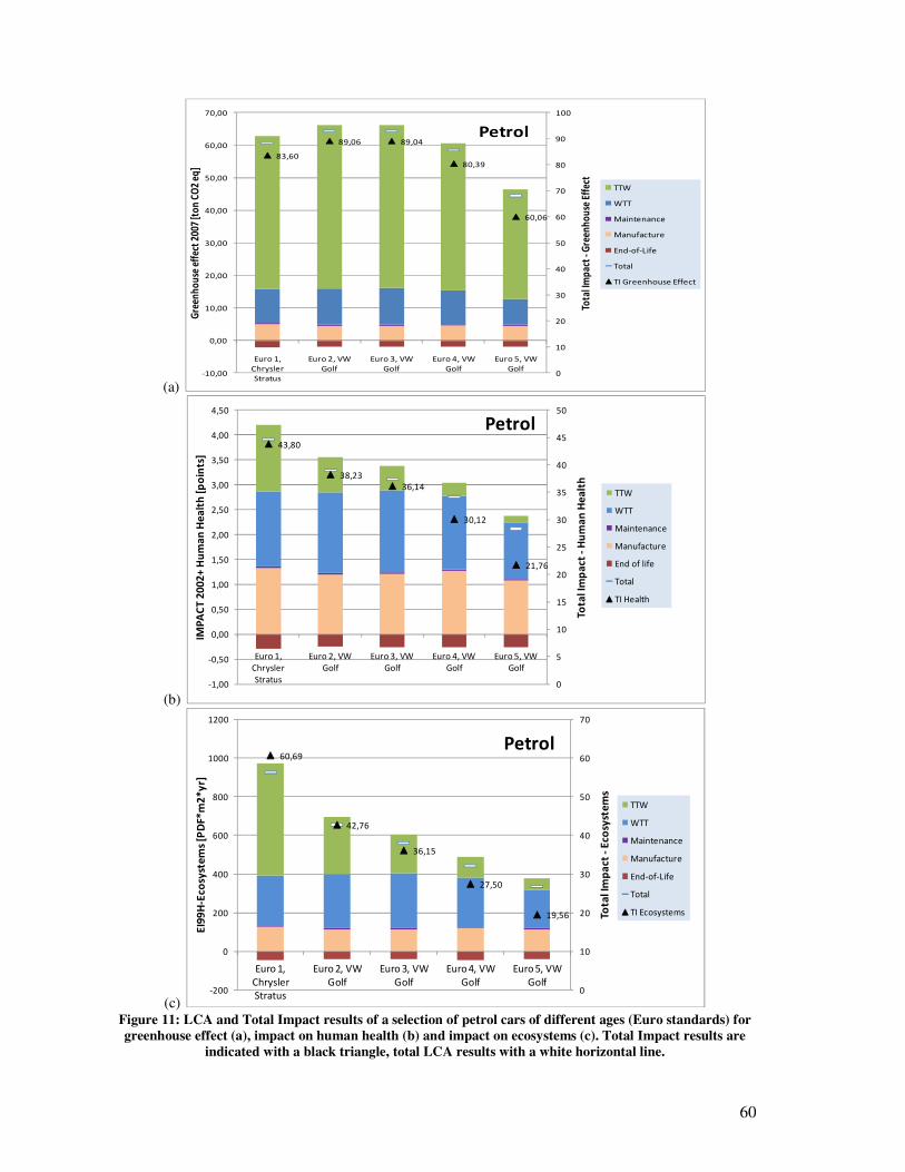
60

(a)

(b)

(c) Figure 11: LCA and Total Impact results of a selection of petrol cars of different ages (Euro standards) for

greenhouse effect (a), impact on human health (b) and impact on ecosystems (c). Total Impact results are

indicated with a black triangle, total LCA results with a white horizontal line.

83,60

89,06 89,04

80,39

60,06

0

10

20

30

40

50

60

70

80

90

100

-10,00

0,00

10,00

20,00

30,00

40,00

50,00

60,00

70,00

Euro 1,

Chrysler

Stratus

Euro 2, VW

Golf

Euro 3, VW

Golf

Euro 4, VW

Golf

Euro 5, VW

Golf

Tota

l Im

pac

t -G

reen

ho

use

Eff

ect

Gre

enh

ou

se e

ffec

t 20

07 [t

on

CO

2 eq

]TTW

WTT

Maintenance

Manufacture

End-of-Life

Total

TI Greenhouse Effect

Petrol

43,80

38,23

36,14

30,12

21,76

0

5

10

15

20

25

30

35

40

45

50

-1,00

-0,50

0,00

0,50

1,00

1,50

2,00

2,50

3,00

3,50

4,00

4,50

Euro 1,

Chrysler

Stratus

Euro 2, VW

Golf

Euro 3, VW

Golf

Euro 4, VW

Golf

Euro 5, VW

Golf

Tota

l Im

pa

ct -

Hu

ma

n H

ea

lth

IMP

AC

T 2

00

2+

Hu

ma

n H

ea

lth

[p

oin

ts]

TTW

WTT

Maintenance

Manufacture

End of life

Total

TI Health

Petrol

60,69

42,76

36,15

27,50

19,56

0

10

20

30

40

50

60

70

-200

0

200

400

600

800

1000

1200

Euro 1,

Chrysler

Stratus

Euro 2, VW

Golf

Euro 3, VW

Golf

Euro 4, VW

Golf

Euro 5, VW

Golf

Tota

l Im

pa

ct -

Eco

syst

em

s

EI9

9H

-Eco

syst

em

s [P

DF*

m2

*y

r]

TTW

WTT

Maintenance

Manufacture

End-of-Life

Total

TI Ecosystems

Petrol

61

(a)

(b)

(c)

Figure 12: LCA and Total Impact results of a selection of diesel cars of different ages (Euro standards) for greenhouse effect (a), impact on human health (b) and impact on ecosystems (c). Total Impact results are

indicated with a black triangle, total LCA results with a white horizontal line.

100,50

66,09

58,0255,65

52,10

-50

-30

-10

10

30

50

70

90

110

-10

0

10

20

30

40

50

60

70

80

Euro 1, Jeep

Cherokee

Euro 2, VW Golf Euro 3, VW Golf Euro 4, VW Golf Euro 5, VW Golf

Tota

l Im

pa

ct -

Gre

en

ho

use

Eff

ect

[p

oin

ts]

Gre

en

ho

use

Eff

ect

20

07

[to

n C

O2

eq

]TTW

WTT

Maintenance

Manufacture

End-of-Life

Total

Diesel

224,62

131,41

86,55

40,77

13,37

-50

0

50

100

150

200

250

-1

0

1

2

3

4

5

6

7

Euro 1, Jeep

Cherokee

Euro 2, VW Golf Euro 3, VW Golf Euro 4, VW Golf Euro 5, VW Golf

Tota

l Im

pa

ct -

Hu

ma

n h

ea

lth

[p

oin

ts]

IMP

AC

T 2

00

2+

Hu

ma

n H

ea

lth

[p

oin

ts]

TTW

WTT

Maintenance

Manufacture

End-of-Life

Total

TI Health

Diesel

100,66

71,39

57,72

33,21

23,30

0

20

40

60

80

100

120

-200

0

200

400

600

800

1000

1200

1400

1600

1800

Euro 1, Jeep

Cherokee

Euro 2, VW

Golf

Euro 3, VW

Golf

Euro 4, VW

Golf

Euro 5, VW

Golf

Tota

l Im

pac

t -E

cosy

stem

s [p

oin

ts]

EI99

H-E

cosy

stem

s [P

DF*

m2*

yr]

TTW

WTT

Maintenance

Manufacture

End-of-Life

Total

TI Ecosystems

Diesel

62

(a)

(b)

(c) Figure 13: LCA and Total Impact results of a selection of different vehicle technologies for greenhouse

effect (a), impact on human health (b) and impact on ecosystems (c). Total Impact results are indicated with

a black triangle, total LCA results with a white horizontal line.

60,06

52,10

66,35

60,63

37,47

15,18

-15

-5

5

15

25

35

45

55

65

-10

0

10

20

30

40

50

60

Petrol (Golf) Diesel (Golf) LPG (Golf) CNG (Zafira) Hybrid (Prius) EV (Leaf)

To

tal Im

pa

ct

-G

ree

nh

ou

se E

ffe

ct

[po

ints

]

Gre

en

ho

use

Eff

ect

20

07

[to

n C

O2

eq

]

TTW

WTT

Maintenance

Manufacture

End-of-Life

Total

TI Greenhouse

Effect

21,76

13,37

8,477,17

14,41

8,44

-20

-10

0

10

20

30

40

50

-1

-1

0

1

1

2

2

3

3

Petrol (Golf) Diesel (Golf) LPG (Golf) CNG (Zafira) Hybrid (Prius) EV (Leaf)

Tota

l Im

pa

ct -

Hu

ma

n H

ea

lth

[p

oin

ts]

IMP

AC

T 2

00

2+

Hu

ma

n H

ea

lth

[p

oin

ts]

TTW

WTT

Maintenance

Manufacture

End-of-Life

Total

TI Health

19,56

23,30

9,81

6,96

10,26

8,80

-10

-5

0

5

10

15

20

25

-200

-100

0

100

200

300

400

500

Petrol (Golf) Diesel (Golf) LPG (Golf) CNG (Zafira) Hybrid (Prius) EV (Leaf) Tota

l Im

pa

ct

-E

co

syst

em

s [p

oin

ts]

EI9

9H

-E

co

syst

em

s [P

DF*

m2

*y

r]

TTW

WTT

Maintenance

Manufacture

End-of-Life

Total

TI Ecosystems

63

IX. Optimal time for replacement

IX.1 Introduction

The energy consumption and the exhaust emissions of new vehicles have decreased

considerably the last years, driven by European emission standards, technological exhaust

treatment improvements and efficient engine technologies. These technological transitions

towards a more sustainable transportation system are encouraged by two main drivers: the

availability of energy sources (political and economical dependence on oil producing countries

and the depletion of the reserve base of fossil fuels) and the negative environmental aspects of

the current transport system [69].

A persistent transition towards a more sustainable transportation sector will involve a mixture

of several options such as: encouraging modal shifts (walking, cycling, public transport), cleaner

vehicle technologies, changing driving behaviour, and controlling the need for motorized

transportation [14].

A way to improve the environmental impact of the transport sector is by replacing old

inefficient vehicles by newer ones. A passenger car in Belgium has a lifetime driven distance

(LTDD) of 230,500 km, which corresponds to 13.7 years [13]. To cover this distance, a smaller

impact on the environment could be obtained by replacing this car before its lifetime with an

environmentally friendlier car. Vehicle replacement is normally driven by economic concerns.

This chapter gives insights in how to introduce environmental aspects in automobile

replacement policies. These policies aim at accelerating the adoption of cleaner vehicles by

taking old vehicles out of the fleet, while supporting the vehicle industry. A scrappage policy

must take the whole life cycle of a vehicle into account. Scrapping an old vehicle and

manufacturing a new one creates additional environmental impacts which must be taken into

consideration. Results of a Life Cycle Assessment (LCA) will be used to check how the Belgian

fleet can evolve towards a greener composition.

IX.2 Methodology

Life Cycle Assessment is a cradle-to-grave approach to determine the total environmental

impact of a product during its life cycle. It includes the extraction of raw materials,

manufacturing, transportation, use and disposal. Since the 90s, LCA is a standardized

methodology [57], [58]. It consists of four phases: goal definition and scoping, inventory

analysis, impact assessment and interpretation.

The goal of this study is to adapt the vehicle fleet to a more ecological composition, in function

of the LCA results. This analysis will be based on the comparison of the well-to-wheel

emissions with the cradle-to-grave (manufacturing, dismantling, recycling and waste treatment)

emissions for vehicles with different ages, Euro standards and technologies. Optimizing

vehicle’s LTDD causes an LCA challenge, combining two contradictory environmental

engineering concepts. Letting a vehicle have a longer use phase avoids specific impacts during

manufacturing, such as mineral extraction damage and energy usage. Product life extension is a

well known DfE (design for environment) strategy [70], [71]. To expand the LTDD the focus

will lie on durability and maintenance. In this case the policy advise would be to replace the old

vehicle as late as possible.

64

Conversely, replacement of an old vehicle with a new, more efficient one, can lower the

impacts introduced during the use phase. Depending on the level of benefit, the policy advise

would be to replace the old car as soon as possible. In this case, the focus will lie on the

development of cleaner vehicle technologies [72].

The optimal time to replace a car depends highly on the market availability of cleaner vehicles.

If an optimization, is to tackle greenhouse gases and there is no car on the market which

consumes considerately less fuel, there is no reason to replace the old vehicle. Moreover, the

CO2 emissions introduced during scrapping an old car and manufacturing a new one would

increase the overall impact on global warming.

To calculate in this case the optimal time of replacement [72] developed a methodology which

takes future developments of cleaner vehicles into account. Today there are cleaner, energy

efficient vehicle technologies available [73]. In this chapter it is discussed what can be done to

optimize the environmental impact of a vehicle today. To differentiate between vehicle

technologies it is investigated how long it takes a new car to have an environmental return on

investment. If we replace an old car today, how fast are we going to feel the benefits? This

period is the environmental breakeven point, the driven distance (or time) at which the

investment of launching a new vehicle starts to have an environmental benefit.

The scope of the study is the Belgian family car fleet. A selection was made of comparable

vehicles with different vehicle technologies (Table 74. LCA seeks to compare the impacts of

different products throughout their lifetime. A functional unit is used to have a comparable

analysis. The chosen functional unit is the use of a passenger car in Belgium over a lifetime

driven distance of 230,500 km corresponding to a vehicle lifespan of 13.7 years [13], [74]. In

this assessment, Ecoinvent [11] default allocation criteria such as energy content, exergy,

weight and unit price are always used for the background system.

Different environmental impacts are considered in this assessment: acidification [62],

eutrophication [62], mineral extraction [63], energy [75], greenhouse effect [61] and respiratory

effects of inorganics [64]. For each specific impact calculation method, only the pollutants

involved in the method are taken into account with respect to the characterization factor

attributed to each pollutant. Of course other impacts will have different results, but the aim is to

develop a theoretical framework to deal with the environmental breakeven point.

IX.3 Inventory

In this study, detailed environmental impacts of the different vehicle technologies are assessed

for the small family car segment. A selection was made of comparable vehicles with different

vehicle technologies (Table 74). The Volkswagen Golf was used as a reference model as it is

available since Euro 2 and is still a popular car on the Belgian market. When no VW Golf

model was available, comparable cars have been chosen from the database. For the CNG

technology, the Opel Zafira was used, for BEV the Nissan Leaf and for petrol hybrid the Toyota

Prius. The Nissan Leaf is considered to have a Lithium battery of 300kg. The Toyota Prius has

a NiMH battery of 56kg.

A far-reaching life cycle inventory step has been elaborated covering all the inputs and outputs

from and to the environment from all the unit processes involved in the product system. No

explicit cut-off criteria have been defined. Whenever possible, all vehicle materials and life

cycle steps have been taken into account. The inventory is, in other words, a broad list of all the

needed materials, chemicals, energies and all the emissions related to the fulfilment of the

functional unit. The life cycle inventory, which was created in the framework of the ‘CLEVER’

project, covers all the life cycle phases of conventional and alternative vehicles [76]. It includes

65

the extraction of raw materials, the manufacturing of components, the assembly, the use phase

(on a well-to-wheel basis) and the end-of-life treatment. When specific Belgian data are not

available, average European data are considered.

Manufacturing

The LCI data of the ‘Golf A4, 1,4l Otto’ [48] used in the ecoinvent database [26] have been

adapted to model the manufacturing phase of all vehicles with respect to their specific weights.

For the hybrid and BEV, the LCI of the Golf A4 has been used to model only the body shell.

Detailed LCI data of different battery technologies for hybrid electric (HEV) and battery

electric vehicles (BEV) have been collected from the SUBAT project [77]. The manufacturing

phase considered in this assessment contains material production, component production,

assembly and transportation to the end-users.

Use phase

The use phase of the vehicles is split up into Well-to-Tank (WTT) and Tank-to-Wheel (TTW).

The WTT part covers the production and the distribution of the fuel while the TTW phase

covers the use of this fuel by the vehicle. Data concerning petrol, diesel and the Belgian

electricity supply mix are gathered from the Ecoinvent database [11]. At the TTW side, the

major part of the data is from the Ecoscore database [14]. It includes technology, weight, fuel

consumption and homologation emissions of all the registered vehicles in Belgium.

Beside the homologation data, heavy metal emissions and non-exhaust particle emissions [49]

are added to the TTW model. Table 74 gives an overview of the tailpipe emissions, fuel

consumption and weight of the different vehicle technologies. The maintenance phase is

modelled as a part of the use phase to calculate the environmental breakeven point. This phase

includes the tyres, the washing water and the lead-acid battery and has been modelled with

inputs from the LCI of the Golf A4 combined with assumptions from the IMPRO-CAR project

[47].

Table 74: Overview of the tailpipe emissions, fuel consumption and weight.

Fuel/

Technology

Euro

standard

Fuel

consumption

[l/100km]

CO2

[g/km]

CO

[g/km]

HC

[g/km]

NOx

[g/km]

SO2

[g/km]

PM

[g/km]

N2O

[g/km]

CH4

[g/km]

Weight

[kg]

Petrol Euro 2 8.9 213 2.200 0.275 0.225 0.00134 0 0.013 0.020 1197

Petrol Euro 5 6.2 144 0.286 0.028 0.045 0.00094 0 0.005 0.020 1215

Diesel Euro 2 6.2 164 1.000 0.070 0.630 0.00105 0.08 0.005 0.010 1333

Diesel Euro 5 4.9 128 0.245 0.040 0.136 0.00083 0.001 0.008 0.010 1264

LPG Euro 5 7.1 169 0.330 0.032 0.012 0.00117 0 0.005 0.020 1247

CNG Euro 5 7.8 139 0.215 0.065 0.022 0 0 0.005 0.124 1660

Hybrid Euro 5 3.9 89 0.258 0.058 0.006 0.00059 0 0.005 0.020 1370

BEV Euro 5 0,15 kWh/km 0 0.000 0.000 0.000 0 0 0 0.000 1587

End-of-life phase

An end-of-life scenario including the transport to the recycling plant, depollution, shredding

and the sorting has been defined in this study. As specified in the EU directive for EoL vehicles

(2000/53/EC), batteries are removed during the depollution step and treated separately. For the

specific case of NiMH and lithium batteries, a pyrometallurgical process has been used to

recover nickel and lithium oxides [51]. Specific rates of material and energy recovery per type

of material which were collected in the framework of the OVAM survey on Belgian recycling

plants, are used [10]. The OVAM survey data reflect the state-of-the-art in Belgium. The

66

recycling efficiency and the recycling process’ energy consumption are taken into account in

the model.

IX.4 Results

Environmental breakeven point

The overall LCA results for a full lifetime driven distance of 230,500 km is given in Table 75

for the different considered impact categories: acidification, eutrophication, mineral extraction,

energy, greenhouse effect and respiratory effects of inorganics. In Table 76, Table 77 and Table

78 this data are subdivided in different life phases (manufacturing, usage, end-of-life treatment)

these tables are used to calculate the environmental breakeven point with equation 3. The

results are divided in the different life phases and the results of the use phase are given per km.

Table 75: Overview of total life cycle impact of the considered vehicle technologies

TOTAL Petrol

Euro 2

Petrol

Euro 5

Diesel

Euro 2

Diesel

Euro 5

CNG

Euro 5

LPG Euro

5

HEV

Euro 5

BEV

Acidification [g SO2 eq.] 1.82E+05 1.20E+05 2.06E+05 1.11E+05 5.68E+04 9.31E+04 9.56E+04 7.93E+04

Eutrophication [g PO4 eq.] 1.93E+04 1.05E+04 2.83E+04 1.21E+04 4.65E+03 8.07E+03 7.35E+03 7.49E+03

Mineral extraction

damage [MJ]

2.02E+03 2.02E+03 2.20E+03 2.08E+03 2.69E+03 2.05E+03 2.35E+03 2.75E+03

Energy [MJ] 9.63E+05 6.95E+05 7.36E+05 5.95E+05 9.12E+05 5.98E+05 4.99E+05 5.26E+05

Greenhouse effect [g CO2

eq.]

6.43E+07 4.45E+07 4.77E+07 3.82E+07 3.98E+07 4.89E+07 3.04E+07 1.67E+07

Respiratory effects

[points]

2.69E+00 1.57E+00 3.33E+00 1.54E+00 9.40E-01 1.34E+00 1.36E+00 1.09E+00

Figure 14: Overview of the impact on climate change for the different vehicle technologies,

after a full lifetime of 230,500kmFigure 15: Cumulative burden on climate change for the

different vehicle technologies give a detailed overview of the impact on climate change for the

different vehicle technologies, after a full lifetime of 230,500km (13.7 years). Figure 14:

Overview of the impact on climate change for the different vehicle technologies, after a full

lifetime of 230,500km shows the division of the LCA results into the different life phases. The

use phase is divided in a well-to-tank (WTT), tank-to-wheel (TTW) and maintenance step. The

petrol Euro 2 vehicle has the largest impact on the greenhouse effect. The petrol vehicle has the

highest fuel consumption, which explains the high WTT and TTW emissions. Thanks to the

hybridization of the drive train, the hybrid vehicle manages to decrease fuel consumption and

accordingly the impact on the greenhouse effect. As a consequence, the hybrid vehicle has the

lowest impact of all internal combustion engine vehicles, considered in this assessment. The

BEV has overall the lowest impact on the greenhouse effect. Figure 15: Cumulative burden on

climate change for the different vehicle technologies gives an insight in the cumulative

environmental burden of a specific vehicle. The first impact at zero driven distance is due to the

manufacturing process. During the usage of a vehicle the cumulative environmental burden

grows per kilometre. The negative values are avoided impacts due to the recovery of materials

in the end-of-life (EoL) recycling step.

67

Figure 14: Overview of the impact on climate change for the different vehicle technologies, after a full

lifetime of 230,500km

Figure 15: Cumulative burden on climate change for the different vehicle technologies

The environmental breakeven point is introduced as the driven distance (or time) at which the

investment producing a new vehicle starts to have an environmental benefit. The environmental

breakeven point (Db) will be dissimilar for each pair of cars and is shown in Figure 16:

Environmental breakeven point of the replacement of a vehicle.. Each impact category will also

give a different set of environmental breakeven points.

Figure 16: Environmental breakeven point of the replacement of a vehicle. shows four choices

when dealing with the replacement of a car, the environmental burden is shown in function of

64

4448

38 40

49

30

17

-10

0

10

20

30

40

50

60

70

Petrol

Euro 2

Petrol

Euro 5

Diesel

Euro 2

Diesel

Euro 5

CNG

Euro 5

LPG Euro

5

HEV

Euro 5

BEV

GH

E [

ton

CO

2e

q]

End-of-Life

Maintenance

TTW

WTT

Manufacturing

Materials

Total

0

10

20

30

40

50

60

70

0 50000 100000 150000 200000 250000

Cu

mu

lati

ve

GH

E [

ton

CO

2e

q]

km driven

Petrol Euro 2

Petrol Euro 5

Diesel Euro 2

Diesel Euro 5

CNG Euro 5

LPG Euro 5

HEV Euro 5

BEV

Production

Recycling

Well-to-wheel (use phase)

68

the time. At time zero the decision is made to replace the car or not. Line 1 (black) shows the

cumulative environmental burden of the decision to keep on using the old vehicle, at the end of

its lifetime it will be recycled. The old car was already manufactured, so the impacts during

manufacturing are not changed by the decision. Therefore, the cumulative environmental

burden of line 1 is only function of the maintenance and the well-to-wheel emissions. Line 2

represents the replacement with a cleaner vehicle, at distance Db the environmental benefit of

replacing the old vehicle starts. The offset of the environmental burden is due to the impact

during manufacturing of the new vehicle, taking the end-of-life treatment and its negative (or

avoided) impacts into account of the old vehicle. In situation 3 the benefit of use phase of the

new vehicle is not big enough to have an environmental return on investment in an appropriate

time frame. In situation 4 the impact of the manufacturing is too big to be compensated by the

use phase, this is especially true when investigating impacts like mineral extraction damage.

The manufacturing of the old car is not allocated to the environmental burden of this car, as it is

not influenced by the replacement decision. The transport, shredding and further separation

processes the old vehicle are allocated to decision 2, 3 and 4. The End-of-Life (EoL) treatment

is based on the state-of-the-art of the Belgian recycling activities [10].

Figure 16: Environmental breakeven point of the replacement of a vehicle.

The environmental breakeven point distance (Db), described in Figure 16: Environmental

breakeven point of the replacement of a vehicle., can be calculated by expressing that the

impact (Ino replacement, Db) of decision 1 (no replacement) is the same as decision 2 (replacement

after Db km) and solving it for Db.

The environmental burden for the “no replacement” scenario at distance Db is given by equation

1.

1, vehicleUsebDbtreplacemenno iDI ⋅= (1)

The environmental burden for the “replacement” scenario at distance Db is given by equation 2.

122., vehicleEoLvehicleUsebvehicleManDbtreplacemen IiDII +⋅+= (2)

With:

Ino replacement, Db the impact for the scenario “no replacement” after Db km”

Ireplacement, Db the impact for the scenario “replacement” after Db km

69

Db environmental breakeven point, expressed in km

iUse, vehicle j the impact per km on the use phase (Well-to-wheel and

maintenance) of vehicle j

IMan, vehicle j the impact of the manufacturing phase of vehicle j

IEoL, vehicle j the impact of the End-of-life treatment phase of vehicle j

The environmental breakeven point can be calculated with equation 3.

kmDb

2 vehicleUse,1 vehicleUse,

1 vehicleEoL,2 vehicleMan,

i - i

I I +=

(3)

In Table 76: Overview of the different environmental impacts of the manufacturing phase,

Table 77: Overview of the different environmental impacts of the use phaseand Table 78:

Overview of the different environmental impacts of the End-of-Life treatment these data are

subdivided in different life phases (manufacturing, usage, EoL treatment). These tables are used

to calculate the environmental breakeven point with equation 3. The results of the use phase are

given per km.

Table 76: Overview of the different environmental impacts of the manufacturing phase

Manufacturing

(IMan, vehicle j)

Petrol

Euro 2

Petrol

Euro 5

Diesel

Euro 2

Diesel

Euro 5

CNG

Euro 5

LPG Euro

5

HEV Euro

5

BEV

Acidification [g SO2

eq.]

4.28E+04 4.34E+04 4.75E+04 4.51E+04 5.89E+04 4.45E+04 7.77E+04 6.71E+04

Eutrophication [g PO4

eq.]

2.95E+03 2.99E+03 3.28E+03 3.11E+03 4.07E+03 3.07E+03 3.98E+03 6.07E+03

Mineral extraction

[MJ]

2.14E+03 2.17E+03 2.38E+03 2.26E+03 2.94E+03 2.23E+03 2.84E+03 2.47E+03


Greenhouse effect [g

CO2 eq.]

4.46E+06 4.53E+06 4.96E+06 4.71E+06 6.16E+06 4.64E+06 6.48E+06 7.56E+06

Respiratory effects

[points]

5.61E-01 5.69E-01 6.23E-01 5.91E-01 7.73E-01 5.84E-01 9.41E-01 8.93E-01

Table 77: Overview of the different environmental impacts of the use phase

Use phase per km

(iUse, vehicle j)

Petrol

Euro 2

Petrol

Euro 5

Diesel

Euro 2

Diesel

Euro 5

CNG

Euro 5

LPG Euro

5

HEV

Euro 5

BEV

Acidification [g SO2 eq.] 6.56E-01 3.81E-01 7.44E-01 3.37E-01 5.89E-02 2.63E-01 2.27E-01 1.86E-01

Eutrophication [g PO4 eq.] 7.66E-02 3.79E-02 1.15E-01 4.49E-02 1.01E-02 2.74E-02 2.17E-02 1.44E-02

Mineral extraction

damage [MJ]

5.71E-04 4.60E-04 4.13E-04 3.70E-04 3.15E-04 3.67E-04 3.66E-04 3.00E-03


Greenhouse effect [g CO2

eq.]

2.68E+02 1.81E+02 1.94E+02 1.54E+02 1.57E+02 2.00E+02 1.14E+02 5.65E+01

Respiratory effects

[points]

9.96E-06 5.05E-06 1.25E-05 4.89E-06 1.70E-06 4.03E-06 3.53E-06 3.18E-06

Table 78: Overview of the different environmental impacts of the End-of-Life treatment

End-of-life

(IEoL, vehicle j)

Petrol

Euro 2

Petrol

Euro 5

Diesel

Euro 2

Diesel

Euro 5

CNG Euro

5

LPG Euro

5

HEV Euro

5

BEV

Acidification [g

SO2 eq.]

-1.15E+04 -1.17E+04 -1.27E+04 -1.21E+04 -1.57E+04 -1.20E+04 -3.45E+04 -3.06E+04

Eutrophication

[g PO4 eq.]

-1.26E+03 -1.28E+03 -1.41E+03 -1.33E+03 -1.75E+03 -1.32E+03 -1.63E+03 -1.89E+03

70

Mineral

extraction

damage [MJ]

-2.53E+02 -2.56E+02 -2.73E+02 -2.63E+02 -3.20E+02 -2.60E+02 -5.81E+02 -4.08E+02

Energy [MJ] -4.05E+04 -4.11E+04 -4.50E+04 -4.27E+04 -5.59E+04 -4.21E+04 -4.96E+04 -7.65E+04

Greenhouse

effect [g CO2

eq.]

-1.84E+06 -1.87E+06 -2.05E+06 -1.94E+06 -2.54E+06 -1.92E+06 -2.29E+06 -3.84E+06

Respiratory

effects [points]

-1.65E-01 -1.67E-01 -1.82E-01 -1.73E-01 -2.25E-01 -1.71E-01 -3.89E-01 -5.40E-01

The environmental breakeven point (Db) for climate change is calculated and presented in

Figure 17: Environmental breakeven points for climate change.. The lines represent the ‘old’

vehicles that are replaced by the new vehicle. The squares represent the environmental

breakeven points. This is where the cumulative impact of the new vehicle crosses the line

representing the old vehicle. As the BEV has the lowest impact on climate change, no other

vehicle has a breakeven point with the cumulative line of the BEV, in the figure this is

represented by the green line without squares. When replacing a petrol Euro 2 vehicle (grey

line) the benefit of the replacement on GHE is obtained after only 5000 kilometres for all types

of vehicles. The replacement of the petrol EURO2 vehicle with a Diesel Euro 5 vehicle has the

earliest benefit, followed by the BEV and the HEV. This is due to the extra impact of the

production of the battery of a BEV. However, after 5000 kilometres, the BEV (green square)

reaches already his breakeven point with the Diesel Euro 5 vehicle (brown line).

Figure 17: Environmental breakeven points for climate change.

0

10

20

30

40

50

0 50000 100000 150000 200000

GH

E [

ton

CO

2e

q]

km driven

Petrol

Euro 2Petrol

Euro 5Diesel

Euro 2Diesel

Euro 5CNG

Euro 5LPG

Euro 5HEV

Euro 5BEV

71

The detailed information of the breakeven points for climate change are given in Table 79. The

environmental breakeven points are given for the replacement of a vehicle in column i with

vehicle in row j. Only positive values are withheld. Values higher than the total lifetime driven

distance (230,500 km) are not in bold, since a higher value means that the replacement will

have no positive effect during the vehicles’ lifetime. For instance, in column 4 the breakeven

points for replacing a diesel Euro 2 vehicle with another vehicle technology are given.

Replacing a diesel Euro 2 vehicle with a diesel Euro 5 vehicle will have a benefit on the GHE

after 65,151 kilometres.

Each impact category will also give a different set of environmental breakeven points, all

impact categories and their corresponding sets of breakeven points are given in Table 79:

Environmental breakeven point for the greenhouse effect when replacing a vehicle in column i

with vehicle in row j and Table 84: Environmental breakeven point for mineral extraction

damage when replacing a vehicle in column i with vehicle in row j.

Table 79: Environmental breakeven point for the greenhouse effect when replacing a vehicle in column i

with vehicle in row j

km Petrol Euro

2

Petrol Euro

5

Diesel Euro

2

Diesel Euro

5

CNG Euro 5 LPG Euro 5 HEV Euro 5 BEV

Petrol Euro

2

- - - - - - - -

Petrol Euro

5

31,150 - 191,292 - - 137,740 - -

Diesel Euro

2

42,587 - - - - 508,445 - -

Diesel Euro

5

25,123 101,888 65,151 - 621,813 59,607 - -

CNG Euro 4 39,083 176,170 110,228 - - 98,011 - -

LPG Euro 4 41,674 - - - - - - -

HEV Euro 5 30,158 68,201 55,011 114,109 91,035 52,715 - -

BEV 27,074 45,512 39,943 57,784 49,823 39,189 91,723 -

72

Table 80: Environmental breakeven point for acidification when replacing a vehicle in column i with vehicle

in row j

km Petrol

Euro 2

Petrol

Euro 5

Diesel

Euro 2

Diesel Euro

5

CNG Euro

5

LPG Euro 5 HEV Euro 5 BEV

Petrol

Euro 2

- - 340,354 - - - - -

Petrol

Euro 5

116,111 - 84,512 - - - - -

Diesel

Euro 2

- - - - - - - -

Diesel

Euro 5

105,203 748,727 79,429 - - - - -

CNG Euro

4

79,321 146,435 67,323 168,411 - 230,052 145,039 223,010

LPG Euro 4 83,971 277,467 66,038 439,597 - - - -

HEV Euro 5 154,384 428,783 125,660 599,945 - 1,846,966 - -

BEV 118,131 283,313 97,274 364,292 - 714,586 785,335 -

Table 81: Environmental breakeven point for eutrophication when replacing a vehicle in column i with vehicle in row j

km Petrol

Euro 2

Petrol

Euro 5

Diesel

Euro 2

Diesel Euro

5

CNG Euro

5


Petrol

Euro 2

- - 40,348 - - - - -

Petrol

Euro 5

44,720 - 20,634 237,445 - - - -

Diesel

Euro 2

- - - - - - - -

Diesel

Euro 5

58,349 - 24,401 - - - - -

CNG Euro

4

42,268 100,246 25,482 78,678 - 159,180 209,852 510,963

LPG Euro 4 36,734 169,876 19,040 99,178 - - - -

HEV Euro 5 49,453 166,163 27,618 113,933 - 467,370 - -

BEV 77,295 203,170 46,466 155,074 - 364,283 602,813 -

Table 82: Environmental breakeven point for energy when replacing a vehicle in column i with vehicle in

row j

km Petrol Euro

2

Petrol Euro

5

Diesel Euro

2

Diesel Euro

5

CNG Euro 5 LPG Euro 5 HEV Euro 5 BEV

Petrol Euro

2

- - - - - - - -

Petrol Euro

5

55,242 - 398,045 - 58,531 - - -

Diesel Euro

2

73,334 - - - 85,991 - - -

Diesel Euro

5

42,642 153,657 108,052 - 41,562 3,912,627 - -

CNG Euro 4 311,664 - - - - - - -

LPG Euro 4 42,190 156,428 108,744 - 40,977 - - -

HEV Euro 5 49,172 106,293 88,880 188,732 49,588 184,042 - -

BEV 75,344 161,543 137,264 284,150 80,402 276,830 8,175,660 -

73

Table 83: Environmental breakeven point for respiratory effects when replacing a vehicle in column i with

vehicle in row j

km Petrol

Euro 2

Petrol

Euro 5

Diesel

Euro 2

Diesel Euro

5

CNG Euro

4


Petrol

Euro 2

- - 146,643 - - - - -

Petrol

Euro 5

82,389 - 51,635 - - - - -

Diesel

Euro 2

- - - - - - - -

Diesel

Euro 5

84,202 2,643,539 53,482 - - - - -

CNG Euro

4

73,634 180,869 54,468 187,981 - 258,582 210,341 157,340

LPG Euro 4 70,654 407,547 47,153 476,083 - - - -

HEV Euro 5 120,642 508,012 84,130 563,224 - 1,538,163 - -

BEV 107,495 388,539 75,960 421,328 - 852,869 1,456,648 -

Table 84: Environmental breakeven point for mineral extraction damage when replacing a

vehicle in column i with vehicle in row j illustrates the environmental breakeven points for the

mineral extraction damage. It is clear that the replacement of a vehicle never has a positive

effect on this impact category, as the manufacturing of a new vehicle will introduces mineral

depletion. Letting a vehicle have a longer use phase avoids this specific impact.

Table 84: Environmental breakeven point for mineral extraction damage when replacing a vehicle in

column i with vehicle in row j

km Petrol

Euro 2

Petrol

Euro 5

Diesel

Euro 2

Diesel Euro

5

CNG Euro

4


Petrol

Euro 2

- - - - - - - 715,58

3

Petrol

Euro 5

17,347,463 - - - - - - 696,52

2

Diesel

Euro 2

13,453,860 45,025,263 - - - - - 762,25

4

Diesel

Euro 5

9,961,716 22,115,730 45,702,721 - - - - 704,54

1

CNG Euro

4

10,478,971 18,436,577 27,089,235 48,688,107 - 51,078,645 46,069,104 943,66

5

LPG Euro 4 9,695,172 21,202,544 42,558,825 779,247,90

2

- - - 692,76

3

HEV Euro

5

12,622,405 27,412,255 54,392,402 681,426,81

5

- 2,046,808,70

4

- 925,29

9

BEV - - - - - - - -

Last distance for replacement

Another interesting point in time to calculate is the ‘Last distance for replacement’, point DL in

Figure 18: Last distance for replacement. DL is defined as the last possible distance to replace

the old vehicle (red line) with a new vehicle (blue line), without polluting more than in the case

of no replacement. This can be seen as the average lifespan of a Belgian vehicle minus the

breakeven point (Db). This approach is only applicable if it is considered that the lifespan of the

particular vehicle is the same as the average lifespan. Beyond DL it is not interesting anymore to

replace the old vehicle because the environmental benefit will be beyond the considered

lifespan. The larger the difference in environmental performance between the old vehicle

(polluter) and its successor (cleaner vehicle) the closer DL can lie to the lifespan. This means

74

one can wait longer to replace the old vehicle, while still having a positive environmental

impact after 13.7 (230,500 km) years. DL can be calculated with equation 4.

Figure 18: Last distance for replacement

bL DkmD −= 500,230 (4)

The total environmental burden after a lifetime driven distance of 230,500 km for the

replacement of an old vehicle (vehicle 1) at distance Dx by a newer vehicle (vehicle 2) is given

by equation 5.

222.111., ) - 500,230( vehicleEoLvehicleUsexvehicleManvehicleEoLvehicleUsexvehicleManDxtotal IiDIIiDII +⋅+++⋅+= (5)

The environmental benefit of replacing an old vehicle at distance Dx is given by ∆IDx. This is

represented in Figure 18: Last distance for replacement by the difference between the

environmental impact of the old vehicle (red line compared to the replacement scenario (green

line). The environmental benefit can be calculated with equation 6.

Dx ,111. 500,230 totalvehicleEoLvehicleUsevehicleManDx IIiII −+⋅+=∆ (6)

With:

Itotal, Dx the total life cycle impact of the decision of replacing a vehicle

after Dx km

Dx distance x, when the replacement is executed

iUse, vehicle j the impact per km on the use phase (Well-to-wheel and

maintenance) of vehicle j

IMan, vehicle j the impact of the manufacturing phase of vehicle j

IEoL, vehicle j the impact of the End-of-life treatment phase of vehicle j

∆IDx environmental benefit of replacing a vehicle at distance Dx,

compared to no replacement.

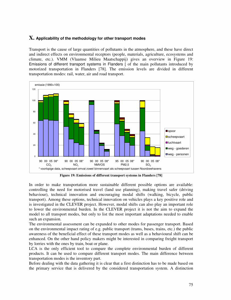
75

X. Applicability of the methodology for other transport modes

Transport is the cause of large quantities of pollutants in the atmosphere, and these have direct

and indirect effects on environmental receptors (people, materials, agriculture, ecosystems and

climate, etc.). VMM (Vlaamse Milieu Maatschappij) gives an overview in Figure 19:

Emissions of different transport systems in Flanders [ of the main pollutants introduced by

motorized transportation in Flanders [78]. The emission levels are divided in different

transportation modes: rail, water, air and road transport.

Figure 19: Emissions of different transport systems in Flanders [78]

In order to make transportation more sustainable different possible options are available:

controlling the need for motorised travel (land use planning), making travel safer (driving

behaviour), technical innovation and encouraging modal shifts (walking, bicycle, public

transport). Among these options, technical innovation on vehicles plays a key positive role and

is investigated in the CLEVER project. However, modal shifts can also play an important role

to lower the environmental burden. In the CLEVER project it is not the aim to expand the

model to all transport modes, but only to list the most important adaptations needed to enable

such an expansion.

The environmental assessment can be expanded to other modes for passenger transport. Based

on the environmental impact rating of e.g. public transport (trams, buses, trains, etc.) the public

awareness of the beneficial effect of these transport modes as well as a behavioural shift can be

enhanced. On the other hand policy makers might be interested in comparing freight transport

by lorries with the ones by train, boat or plane.

LCA is the only efficient tool to compare the complete environmental burden of different

products. It can be used to compare different transport modes. The main difference between

transportation modes is the inventory part.

Before dealing with the data gathering it is clear that a first distinction has to be made based on

the primary service that is delivered by the considered transportation system. A distinction

0

20

40

60

80

100

120

90 00 05 08* 90 00 05 08* 90 00 05 08* 95 00 05 08* 90 00 05 08*

emissie (1990=100)

spoor

scheepvaart

luchtvaart

weg - goederen

weg - personen

CO2 NOx NMVOS PM2,5 SO2

* voorlopige data, scheepvaart omvat zowel binnenvaart als scheepvaart tussen Noordzeehavens

76

between passenger and freight transportation is needed, because this will influence the

Functional Unit. The Functional Unit is a quantified description of the performance of product

systems, for use as a reference unit. It allows comparing two or several product systems on the

basis of a common provided service. In the Clever framework, the functional unit is defined as

driving with a passenger vehicle for a full Life Time Driven Distance (LTDD) of 230,500 km.

When comparing different transport modes for passengers, this LTDD is not solely applicable

anymore as Functional Unit. When comparing different passenger transport modes (car, train,

air plane, bus metro, tram) it is necessary to take the occupancy into account. The Functional

unit should be written passenger kilometres (p.km). For freight transport the Functional Unit

should include the weight of the goods that are transported (ton.km).

Since the methodology defined in the CLEVER project also includes background processes,

such as the production of fuel (petrol, diesel, electricity, …) and materials (steel, copper,

plastics, …) and their respective emissions the methodology can be extended to other transport

modes.

When the BOM (Bill-of-Material) is available for the considered vehicles (e.g. train, urban

busses) the cradle-to-grave emissions (related directly and indirectly to vehicle production and

end-of-life processing of the vehicle) can be modelled in the same way as a passenger car.

The Well-to-Tank (WTT) part is already available from the inventory made in the CLEVER

project, but must be completed with the specific energy usage and tailpipe emissions from the

Tank-to-Wheel part of the use phase of a vehicle.

For the impact calculation itself it is suggested to use the same impact categories as in the

CLEVER report. Retained classes are acidification, eutrophication, greenhouse gases, chemical

toxicity indicators, depletion of the ozone layer, consumption of renewable and non-renewable

energy and depletion of minerals.

XI. Main conclusions of the LCA

Comparing the environmental impact of conventional vehicles (diesel, petrol) has already

shown to be a difficult exercise. Diesel cars for example are more fuel efficient and emit less

greenhouse gases than petrol cars, but on the other hand emit more particulate matter and NOx,

which have a strong impact on human health. Many environmental rating tools exist which are

able to give an environmental score to different vehicle technologies, but which provide

different results due to the many methodologies and weighting parameters that can be used. The

Ecoscore methodology is an example of such a rating tool, which is based on a well-to-wheel

approach, implying that both tailpipe and indirect emissions due to the fuel or electricity

production and distribution are taken into account.

The comparison becomes even more complex with the introduction of so-called ‘alternative’

fuels and drive trains (LPG, CNG, HEV, BEV, FCEV, biofuels, hydrogen). To make a fair

comparison of all these fuels and technologies, not only the well-to-wheel emissions should be

considered, but also the emissions due to the production, maintenance and end-of-life phase of

the vehicle. In electric vehicles for instance, large batteries or a fuel cell are used, which are not

present in conventional ICE vehicles and which can have a significant environmental impact.

To take all these life cycle phases and emissions into account, a Life Cycle Assessment (LCA)

has been performed on a wide range of vehicles which are available on the Belgian market.

LCA is an ISO-certificated methodology, which is generally used to compare products or

services on a comparable basis. In the CLEVER project, an LCA methodology has been

developed with a per-model applicability instead of an average vehicle LCA. This allows taking

77

into account all segments of the Belgian passenger car market (family car, SUV, city car, etc.)

and producing LCA results per vehicle technology and category. These vehicles were compared

on the basis of the same provided service to the user, which has been defined as the use of a

passenger car in Belgium during 13, 7 years and a lifetime driven distance of 230.500 km.

Because of the large variety of environmental impact categories, it is almost impossible and

sometimes misleading to claim that a vehicle is better than the others from all viewpoints. In

this project, a list of relevant environmental impact categories has been made in order to have a

good appreciation of the environmental score of conventional and alternative vehicles. The

impact calculation methods used in this project are: the IPCC 2007 Greenhouse Effect, The

respiratory effect from Impact 2002+, air acidification and eutrophication from ‘Centrum voor

Milieukunde Leiden’ (CML), the mineral extraction damage from Eco-indicator and the

consumption of renewable and non-renewable energy.

When dealing with climate impact, conventional vehicles have the highest impact. On average,

diesel vehicles always score better than petrol vehicles but the sensitivity analysis reveals a

strong overlap between these two technologies. BEV powered with the Belgian supply mix

electricity, with the exception of the sugar cane based E85 vehicle, has a lower greenhouse

effect than all the registered family cars in Belgium. However, extreme scenarios, where

electricity produced from 100% coal or oil is considered, give higher eutrophication and

acidification impacts to the BEV. Moreover, the climate benefit of the use of nuclear and

renewable electricity in BEV as well as the maintaining of this benefit when the energy

consumption increases has been demonstrated.

In general, biofuels have lower CO2 emissions due to the CO2 uptake during the photosynthesis

of the organic matter. However, this benefit of the CO2 uptake can be balanced by N2O

emissions deriving from nitrogen contained in fertilizers. So the type of feedstock used to

produce biofuels and the agricultural practices have a strong influence on the climate impact of

biofuels. Contrarily to climate impact, first generation bio-fuels have a bad respiratory effect

(Sugar cane ethanol and RME) and bad acidification (RME) scores because of nitrogen-based

emissions (NH3 and NOx) and/or sometimes PM emissions. However, a vehicle using sugar

beet ethanol will have a respiratory effect and an acidification impact which are comparable to

conventional cars. Again, the type of feedstock used to produce the biofuel is the main

influencing parameter of its environmental score. Close to the feedstock type, the agricultural

practices also influence the environmental score of biofuel vehicles. For example, the

respiratory effect score of sugar cane ethanol can be highly improved by avoiding burning the

sugar cane before the harvest. This is why the development and production of second

generation biofuels need to be encouraged. It is important to notice that petrol and diesel

vehicles are better than respectively ethanol and biodiesel vehicles for respiratory effects

(inorganics). For the acidification impact, petrol and ethanol vehicles are comparable while

diesel vehicles are clearly better than RME vehicles.

The use of mineral resources is also a key issue in the manufacturing, the use and the

maintenance of vehicles. For this impact category, the size of a vehicle and the use of specific

components requiring specific materials are the influencing parameters. Hybrid vehicles and

FCEV will have a higher impact for this indicator because of the use of specific and rare

materials to produce components like the NiMH battery, fuel cell and hydrogen tank. The BEV

has slightly lower mineral resource damage but the contribution of the battery is still high.

Another finding for this indicator is the high contribution of the transport and distribution of the

electricity used to power the BEV. This is essentially due to the use of copper in the electric

78

cables. It is important to mention that an increase of the size of a BEV will quickly increase its

mineral extraction damage. The RME vehicle has an impact higher than petrol and diesel and

comparable to hybrid and FCEV. This is mainly due to the use of mineral fertilizers during the

rape production. Petrol, diesel and ethanol vehicles have comparable results and have the best

scores after BEV and CNG.

This study has also revealed how important recycling is especially for heavy and precious

metals contained in specific components such as batteries and fuel cells (FCEV, Hybrid,

BEV…).

For the different impact categories considered in this study, the impacts of LPG technology are

comparable to diesel. However, better environmental scores are possible for LPG by using for

example flare gas instead butane/propane from oil refinery to produce LPG.

FCEV are more interesting than petrol and diesel vehicles for greenhouse effect, respiratory

effect and acidification. This is mainly due to the fact that the FCEV is a TTW emission-free

(except water vapour) vehicle and the fact that the hydrogen is produced with natural gas via

steam methane reforming. In fact natural gas has a very low acidification impact and respiratory

effect. However, the steam reforming process used to produce the hydrogen is energy intensive.

As a consequence, the FCEV has a bigger WTT greenhouse effect despite its interesting overall

greenhouse score. The above mentioned environmental benefits of a FCEV are only applicable

when producing hydrogen from methane. Producing hydrogen through electrolysis has a high

environmental impact due to the energy intensity of this reforming step.

Another interesting finding of this study is that CNG vehicles appear to be an interesting

alternative for conventional vehicles. It has a low climate impact (comparable to hybrid

technology) and the best score for respiratory effects and acidification. It also has the lowest

mineral extraction damage after BEV. However CNG is produced with a fossil fuel. So, CNG

vehicles will become more interesting with the development of the biomethane sector.

Finally, it appears in this study that the vehicle segment has a strong influence on the LCA

results. In general, the bigger the segment (e.g. from supermini to large family car), the worse

the environmental score. Additionally, when comparing the results for the different vehicle

segments, the trends between the different vehicle technologies remain the same.

The results of the LCA were compared with the results of the Ecoscore methodology

(calculated as Total Impact) for different vehicle technologies and different ages within the

same technology. Since the Ecoscore has to be calculated for all available vehicles, it is limited

by the fact that only the emissions due to the well-to-wheel phases of the vehicle are readily

available and can be used as a basis to calculate their environmental impact. The LCA

methodology on the other hand, is not limited by these restrictions and offers the possibility to

show very detailed results and this for a large range of impact categories. Therefore LCA can

give a more profound image of the actual environmental impact of a vehicle.

Taking into account these considerations, the Ecoscore methodology has proven to be a good

approach to estimate a vehicle’s environmental impact, since the ranking of vehicles regarding

their environmental performance will not be altered between both assessment methodologies.

The influence of neglecting the impact of the manufacturing, maintenance and end-of-life

phases has shown to be very small, especially for the conventional vehicle technologies (petrol,

diesel, LPG). For hybrid and battery electric vehicles, the manufacturing and end-of-life of the

battery also plays an important role, which is mainly displayed in the impact on human health

79

and ecosystems. However, since the impact on global warming counts for 50 % in the final

Ecoscore, these differences will play a smaller role and still lead to the same ranking of the

vehicle technologies as in the LCA results for greenhouse effect.

This proves that the well-to-wheel approach used in the Ecoscore methodology is a solid basis

for the environmental assessment of different vehicle technologies. The LCA methodology is

an ideal tool to go deeper into these results and provide a thorough insight into the different

impacts of a vehicle.

The environmental breakeven point is introduced as the driven distance (or time) at which the

investment of launching a new vehicle starts to have an environmental benefit. The

environmental breakeven point will be dissimilar for each pair of cars. A methodology and data

is provided to calculate the environmental breakeven point for different types of vehicle

technologies and impact categories. The included impact categories are: acidification,

eutrophication, mineral extraction, energy, greenhouse effect and respiratory effects of

inorganics.

The considered electric vehicle has the lowest impact on climate change and consequently it

can replace every considered car when dealing with this impact category and have a positive

effect after a distance ranging from 27,000 km (when replacing a Petrol Euro 2 vehicle) to

91,000 km (when replacing a fuel efficient hybrid Euro 5 vehicle). It is clear that in this

situation the environmental breakeven point falls in the Life Time Driven Distance of 230,500

km (average life time of a vehicle in Belgium). Hybrid vehicles can replace all other

technologies (except BEV) and still have a positive influence before the end-of-life.

Each impact category will give a different set of environmental breakeven points. The CNG

vehicle has the best performance when dealing with respiratory effects. Nonetheless, the

environmental breakeven point is mostly to far away in time to really provide an environmental

benefit when replacing an old vehicle. This is especially true when trying to replace cleaner

vehicle technologies such as LPG, hybrid and electric vehicles. Old Diesel Euro 2 vehicles, do

not have a particulate filter. Due to their high PM and NOx emissions, it is always beneficial to

replace such a vehicle with another vehicle technology.

When introducing automobile replacement policies in order to accelerate the adoption of

cleaner vehicles by taking old vehicles out of the fleet, one must bear in mind that such a

scrappage policy is focussing on reducing environmental impacts introduced during the use

phase. The policy advise would be to replace the old vehicle as soon as possible with a cleaner

vehicle technology in order to maximise the environmental benefits.

Conversely, letting a vehicle have a longer use phase avoids specific impacts during

manufacturing, such as mineral extraction damage. It is clear that the replacement of a vehicle

cannot have a positive effect on this impact category, as the manufacturing of a new vehicle

will always introduces mineral usage and depletion. Letting a vehicle have a longer use phase

avoids this specific impact. To expand the LTDD the focus will lie on durability and

maintenance. In this case the policy advise would be to replace the old vehicle as late as

possible.

The ‘Last distance for replacement’, is introduced and defined as the last possible distance to

replace an old vehicle with a new vehicle, without polluting more than in the case of no

replacement. This can be seen as the average lifespan of a Belgian vehicle minus the breakeven

point. Beyond the ‘Last distance for replacement’ it is not interesting anymore to replace the old

vehicle because the environmental benefit will not take place in the considered lifespan.

Finally, the environmental benefit of replacing an old vehicle at a certain moment during its

lifecycle is being defined by the difference between the environmental impact of the old vehicle

compared to the replacement scenario.

References

[1] EUCAR/JRC/CONCAWE, Well-to-Wheels analysis of future automotive fuels and powertrains in the

European context, 2006.

[2] European Commission, Directorate-General for Research/IER University of Stuttgart, Extern E-

Externality of Energy, 2005.

[3] De Ruyck J., Lavric D., Bram S., Navak A., Jossart J-M., Remacle M-S., Palmers G., Dooms G.,

Hamelinck C., Liquid Bio-fuels in Belgium in a global Bio-energy context, January 2005.

[4] European Comission, PREMIA: Measures for the promotion of bio-fuels, May 2007.

[5] SGS-Ingenieure,Okologischer vergleich voor rapsöl mit RME und Stellungnahme, October 2001.

[6] SenterNovem, Particpative LCA on Bio-fuels, Report 2 GAVE-05.08, 2005.

[7] Lane B., Life Cycle Assessment of vehicle fuels and technologies, March 2006.

[8] VITO & 3E, Biobrandstoffen in Vlaanderen, February 2006.

[9] SUBAT, « Sustainable batteries », project funded by the European Commission http://www.battery-

electric.com/documents.php , 2004

[10] OVAM, IBGE/BIM, OWD en RDC Environment, Validation of the recycling rates of end-of life

vehicles, June 2008.

[11] Swiss Centre for Life Cycle, ecoinvent Data V2.01, CD-ROM, ISBN 3-905594-38-2, Dubendorf, 2007

[12 ] http://statbel.fgov.be/fr/statistiques/chiffres/circulation_et_transport/circulation/distances/index.jsp,

visited on July 22, 2010

[13] FEBELAUTO, rapport annuel 2006.

[14] Timmermans J-M. Matheys J., Van Mierli J., Lataire P., Environmental rating of vehicles with different

fuels and drive trains: a univocal and applicable methodology, European

journal of transport and infrastructure research, 6(4), pp. 313-334, 2006

[15] The European Parliament and the Council of the European Union, Directive 98/69/EC relating to

measures to be taken against air pollution by emissions from motor vehicles, 1998.

[16] Sergeant N. 1, Boureima F.-S., Matheys J., Timmermans J.-M. & Van Mierlo J., An environmental

analysis of FCEV and H2-ICE vehicles using the Ecoscore methodology, World Electric Vehicle

Journal Vol. 3, ISSN 2032-6653, 2009

[17] Chasserot M., Integrated approach to mobile air conditioning testing and labeling, European

Commission’s Public Consultation: reaching the 130 g/km objective through vehicle technology,

July 2007

[18 ] Council of the European Communities, Directive 92/21/EEC on Masses and dimensions of motor

vehicles of category M1, March 1992

[19] Frischknecht R., Jungbluth N., Althaus H-J., Doka G., Dones R., Heck T., Hellweg S., Hischier R.,

Nemecek T., Rebitzer G. and Spielmann M., The ecoinvent Database: Overview and methodological

framework, International Journal of LCA, 2004

[20] Frischknecht R., Niels Jungbluth N., Althaus H-J., Doka G., Dones R., Heck T., Hellweg S., Hischier

R., Nemecek T., Rebitzer G.; Spielmann M.; Wernet G.,Overview and methodology, ecoinvent report

No.1; 2007

[21] http://www.fcai.com.au/, Visited on 09 September ,2008

[22] www.euroncap.com visited on July 25, 2007

[23] www.fisita.com, Visited on September 9, 2008

[24] Reniers J., FEDERAUTO Magazine, Aout/September 2007

[25] www.ecoscore.be, visited on 3rd

Jully 2010

[26] Spielmann M., Bauer C., Dones R., Tuchschmid M., Ecoinvent report no 14 : Transport services, Data

V2.0, Villigen and Uster, December 2007.

[27] Kudoh Y., Nansai K., Kondo Y., Tahara K., Life Cycel CO2 emissions of FCEV, BRV and GV in

actual use, EVS 23 proceedings, Anaheim, 2007

[28] http://automobiles.honda.com/fcx-clarity/specifications.aspx, visited on March 9, 2009

[29] Product ecology consultants, SimaPro 7.1.8, 2008, The Netherlands

[30] Strauss k., Brent A. C., Hietkamp S., Characterization and Normalization factors for life cycle impact

assessment –Mined Abiotic Resources Categories in South Africa-The manufacturing of catalytic

converter exhaust system as a case study, International journal of LCA , November 2006

[31] Amatayakul W, Ramnäs O, Life cycle assessment of a catalytic converter for passenger cars , Journal of

Cleaner Production , September 2001

82

[32] Dones R., Bauer C., Bolliger R., Burger B., Roder A., Faist-Emmenegger M., Frischnecht R, Jungbluth

N., Tuchschmid M., Ecoinvent report No 5: Life cycle inventories of energy systems: results for current

systems in switzerland and other UCTE countries, Villigen and Uster, December 2007.

[33] Boureima F., Sergeant N., Messagie M., Wynen V., Well-to-Wheel analysis of new vehicle

technologies for future vehicle markets, Study performed by ETEC for Electrabel, Confidential,

December 2009

[34] http://economie.fgov.be/energy/energy_statistics/Statistics_fr_005.htm , visited on 29 July 2008

[35] Faist-Emmenegger M., Heck T, Jungbluth N., Tuchschmid M.,Ecoinvent report No 6 : Erdgas, Data

V2.0, Villingen ,December 2007.

[36] Prieur A., Favreau D., Vinot S., Well-to-Tank technology pathways and carbon balance, Deliverable

4.3, Roads2hycom project, January 2009

[37] Althaus H.-J., Chudacoff M., Hischier R., Jungbluth N., Osses M., Primas A.,Helleweg S., Ecoinvent

report No 8, Life cyle invsntories of chemicals,Dubendorf, December 2007

[38] Jungbluth N,, Ecoinvent report No 6, Part 4, Erdoel, Data V2.0, Uster, 2007

[39] www.wikipedia.org , visited on 31 July 2008

[40] CONCAWE, EUCAR, JRC, 2007, Well-to-Wheels analysis of future automotive fuels and power trains

in the European context”, Well-to-Wheels Report, version 2c

[41] http://wps.com/LPG/WVU-review.html , visited on 5 August 5 2008

[42] AEGPL-Europe, Automotive LPG-Autogas: A competitive alternative fuel for improving air quality,

2004

[43] Niels Jungbluth N., Faist-Emmenegger M ,Dinkel F., Doka G., Chudacoff M., Dauriat A.,Spielmann

M., Sutter J., Kljun N., Keller M., Schleiss k., Ecoinvent report No.17: Life Cycle Inventories of

Bioenergy, Uster , December 2007

[44] Van Den Bossche P., Vergels F., Van Mierlo J., Matheys J., Van Autenboer W., SUBAT: an assessment

of sustainable battery technology, Journal of power sources, Volume 162. Issue 2, November 2006

[45] HyHeels – Hybrid High Energy Electrical Storage, EC 6th Framework Programme, , coordinated by

Siemens VDO Automotive and 11 partners.

[46] Teslamotors, http://www.teslamotors.com/blog2/?p=39, accessed on September 16, 2010

[47] Nemry F., Leduc G., Mongelli I.,Uihlen A., Environmental Improvement of Passenger cars(IMPRO-

car), JRC-European Comission, 2008

[48] Schweimer G. W, Levin M., Life Cycle Inventory for the Golf A4, 2000

[49] European Environment Agency, CORINAIR: the Core Inventory of Air Emission in Europe,

Atmospheric Emission Inventory Guidebook, December 2006

[50] Hischier R., Ecoinvent report no 18, part V: Disposal of electronic and electric equipment, Swiss centre

for life cycle inventories, St-Gallen, 2007

[51] Fisher k:, Wallén E:, Laenen P-P; Collins M.; Battery Waste Management Life Cycle Assessment;

final report for publication; commissioned by the UK department for environment, food and rural

affairs (Defra), October 2006

[52] Michael S, Hans-Jörg A, Can a prolonged use of passenger reduced environmental burdens?, Journal of

Cleaner Production, 2007

[53] Biofuel Sustainable End Uses (BIOSES), funded by the Belgian science policy in the framework of

science for sustainable development (SSD), 2007-2010

[54] Szwabowski S J., Hashemi S., Stockhausen W F., Natkin R J., Reams l., Kabat D M., Potts C., ‘ Ford

Hydrogen Engine Powered P2000 Vehicle’ SAE technical paper series, Ford Motor Co., World

Congress, Detroit Michigan, 2002

[55] http://automobiles.honda.com/fcx-clarity/specifications.aspx , visited on September 10, 2008

[56] IBGE-BIM/Guignard Aude, Timmermans Jean Marc, « Coûts financiers directs et indirects engenders

par l’installation de systèmes d’air climatisé dans les voitures particulières », february 2005

[57] International; Standardisation Organisation, Environmental management - Life cycle assessment -

Principles and framework (ISO 14040:2006), Geneva, 2006

[58] International; Standardisation Organisation, Environmental management - Life cycle assessment -

Requirements and Guidelines (ISO 14044:2006), Geneva, 2006

[59] European Commission, Joint Research Centre, ILCD Handbook, International Reference Lifce Cycle

Data System,: General Guide for Life Cycle Assessment-Detailed Guidance, Ispra, 2010

[60] European Commission, Joint Research Centre, ILCD Handbook, International Reference Lifce Cycle

Data System,: Analysis of Existing Environmental Impact Assessment Methodologies for Use in Life

Cycle Assessment , Ispra, 2010

[61] IPCC Fourth Assessment Report. Climate Change 2007. The Physical Science Basis.

http://www.ipcc.ch/ipccreports/ar4-wg1.htm

83

[62] Guinée J. B., Gorrée M., Heijungs R., Huppes G., Kleijn R., de Koning A., van Oers L., Wegener

Sleeswijk A., Suh S., Udo de Haes H. A., de Bruijn H., van Duin R., Huijbregts M. A. J., Lindeijer E.,

Roorda A. A. H., Weidema B. P., Life cycle assessment; An operational guide to the ISO standards;

Parts 1 and 2. Ministry of Housing, Spatial Planning and Environment (VROM) and Centre of

Environmental Science (CML), Den Haag and Leiden, The Netherlands, retrieved

from:http://www.leidenuniv.nl/cml/ssp/projects/lca2/lca2.html.

[63] Goedkoop M. Spriensma R. (1999a) The Eco-indicator 99: A damage oriented method for life cycle

impact assessment. PRé Consultants, Amersfoort, 1999 [64] Jolliet O., Margni M., Charles R., Humbert S., Payet J., Rebitzer G., Rosenbaum R., IMPACT 2002+: A

New Life Cycle Impact Assessment Methodology, International Journal of Life Cycle Assessment, 8(6),

pp.324-330, 2003

[65] Moreira J. R., Sugarcane for energy, recent results and progress in Brazil, Energy for sustainable

development, 200

[66] Estado Sao Paolo, Lei 11241/02 | Lei nº 11.241, de 19 de setembro de 2002 de São Paulo, Dispõe sobre

a eliminação gradativa da queima da palha da cana-de-açúcar e dá providências correlatas, 2002.

[67] European Commission (1999). Methodolgy for calculating transport emissions and energy consumption

(MEET). Transport research, Fourth Framework Programme, Strategic Research, DG VII – 99,

Luxembourg.

[68] ExternE project (1997). Externalities of Energy, fol. 2 – Methodology. A report produced for the

European Commission, DG XII, Luxembourg.

[69] Van Mierlo J. & Macharis C. (2005). Goederen- en Personenvervoer: Vooruitzichten en Breekpunten,

(Freight and passenger transport: prospects and breaking points), Garant, ISBN 90-441-4908-7, 579p

[70] Keoleian G., Menerey D. (1993). Life Cycle Design Guidance Manual: Environmental Requirements

and The Product System; U.S. Government Printing Office: Washington, DC, EPA600-R-92-226.

[71] Stahel, W. R. (1994). In The Greening of Industrial Ecosystems; Allenby, B. R., Richards, D. J., Eds.;

NationalAcademyPress: Washington, DC, pp 178-190.

[72] Kim H. C., Keoleian G., Grande D., Bean J. (2003). Life cycle optimization of automobile replacement:

model and application, Environ. Sci. Technol. 5407-5413.

[73] Messagie M., Boureima F., Sergeant N., Matheys J., Turcksin L., Macharis C. and Van Mierlo J.

(2010). ‘Life Cycle Assessment of conventional and alternative small passenger vehicles in Belgium’,

IEEE VPPC 2010, Vehicle Power and Propulsion Conference, Lille, France, 1-3 September 2010.

[74] FPS Economy (2010).

http://statbel.fgov.be/fr/statistiques/chiffres/circulation_et_transport/circulation/distances/index.jsp,

accessed on July 22, 2010

[75] VDI. (1997), "Cumulative Energy Demand - Terms, Definitions, Methods of Calculation." VDI-

Richtlinien 46000.

[76] Van Mierlo J., Boureima F., Sergeant N., Wynen V. , Messagie M.,Govaerts L., Denys T.,

Vanderschaeghe M.,Macharis C., Turcksin L., Hecq W., Englert M.,Lecrombs F.,Klopfert F.,De Caevel

B., De Vos M. Clean Vehicle Research: LCA and policy measures (Clever), Final report Phase two.

Brussels, Belgium: Belspo:

'http://www.belspo.be/belspo/ssd/science/Reports/CLEVER_Finalreport_phaseI_ML.pdf', 2011.

[77] Matheys J., Timmermans J., Van Mierlo J., Meyer S., Van Den Bossche P., Comparison of the

environmental impact of 5 electric vehicle battery technolgies using LCA., International Journal of

sustainable manufacturing, pp 318-329, ISBN-ISSN: 1742-7223, 2009.

[78] VMM (2007). Milieurapport Vlaanderen MIRA. Achtergronddocument sector transport.

Clean Vehicle Research: LCA and Policy Measures (CLEVER)

(Report of task 2.1)

LCA software selection

Department of Electrotechnical Engineering and Energy Technology (ETEC)


Authors:

Study realised by: Faycal-Siddikou Boureima,

Nele Sergeant

Vincent Wynen

Under the supervision of Prof .Dr. Ir. Joeri Van Mierlo June, 2007

Table of contents

1. Introduction ............................................................................................................................................................. 1

2. The preselection ....................................................................................................................................................... 1

3. The selection............................................................................................................................................................. 1

3.1. The questionnaire ........................................................................................................................ 2

3.2. Synthesis of the answers .............................................................................................................. 3

3.3. Demonstrations ............................................................................................................................ 7 3.3.1. Gabi ......................................................................................................................................... 7 3.3.2. SimaPro ................................................................................................................................... 7 3.3.3. TEAM ..................................................................................................................................... 7 3.3.4. RangeLCA .............................................................................................................................. 7

4. Conclusion ................................................................................................................................................................ 8

Appendix: Questionnaire ................................................................................................................................................. 9

1. Overview ................................................................................................................................................................ 10

2. Supported ............................................................................................................................................................... 10

2.1. Supported, updated .................................................................................................................... 10 2.1.1. Gabi 4 .................................................................................................................................... 10 2.1.2. SimaPro 7 .............................................................................................................................. 10 2.1.3. TEAM 4.0 ............................................................................................................................. 10 2.1.4. RangeLCA 2.1 ...................................................................................................................... 10

2.2. Service hotline ........................................................................................................................... 10 2.2.1. Gabi 4 .................................................................................................................................... 10 2.2.2. SimaPro 7 .............................................................................................................................. 10 2.2.3. TEAM 4.0 ............................................................................................................................. 11 2.2.4. 1.2.4 RangeLCA 2. ............................................................................................................... 11

2.3. The training ............................................................................................................................... 11 2.3.1. Gabi 4 .................................................................................................................................... 11 2.3.2. SimaPro 7 .............................................................................................................................. 11 2.3.3. TEAM 4.0 ............................................................................................................................. 12 2.3.4. RangeLCA 2.1 ...................................................................................................................... 12

3. Functionality .......................................................................................................................................................... 12

3.1. Minimal requirements ................................................................................................................ 12 3.1.1. Gabi 4 .................................................................................................................................... 12 3.1.2. SimaPro 7 .............................................................................................................................. 13 3.1.3. TEAM 4.0 ............................................................................................................................. 13 2.1.4 RangeLCA 2.1 ............................................................................................................................ 14

3.2. Microsoft Windows operation system ........................................................................................ 14 3.2.1. Gabi 4 .................................................................................................................................... 14 3.2.2. SimaPro 7 .............................................................................................................................. 14 3.2.3. TEAM 4.0 ............................................................................................................................. 14 3.2.4. RangeLCA 2.1 ...................................................................................................................... 14

3.3. The size and the complexity of the process model...................................................................... 14 3.3.1. Gabi 4 .................................................................................................................................... 14

9

3.3.2. SimaPro 7 .............................................................................................................................. 14 3.3.3. TEAM 4.0 ............................................................................................................................. 15 2.3.4 RangeLCA 2.1 ............................................................................................................................ 15

3.4. Inventory and impact assessment ............................................................................................... 15 3.4.1. Gabi 4 .................................................................................................................................... 15 3.4.2. SimaPro 7 .............................................................................................................................. 15 3.4.3. TEAM 4.0 ............................................................................................................................. 15 3.4.4. RangeLCA 2.1 ...................................................................................................................... 15

3.5. Graphical interface .................................................................................................................... 15 3.5.1. Gabi 4 .................................................................................................................................... 15 3.5.2. SimaPro 7 .............................................................................................................................. 15 3.5.3. TEAM 4.0 ............................................................................................................................. 15 3.5.4. RangeLCA 2.1 ...................................................................................................................... 16

3.6. Import and export possibilities (from/to MS Office tools? Others?).......................................... 16 3.6.1. Gabi 4 .................................................................................................................................... 16 3.6.2. SimaPro 7 .............................................................................................................................. 16 3.6.3. TEAM 4.0 ............................................................................................................................. 16 3.6.4. RangeLCA 2.1 ...................................................................................................................... 16

3.7. Possibility to change impact factors .......................................................................................... 16 3.7.1. Gabi 4 .................................................................................................................................... 16 3.7.2. SimaPro 7 .............................................................................................................................. 17 3.7.3. TEAM 4.0 ............................................................................................................................. 17 3.7.4. RangeLCA 2.1 ...................................................................................................................... 17

3.8. Possibility to change weighting factors ..................................................................................... 17 3.8.1. Gabi 4 .................................................................................................................................... 17 3.8.2. SimaPro 7 .............................................................................................................................. 17 3.8.3. TEAM 4.0 ............................................................................................................................. 17 3.8.4. RangeLCA 2.1 ...................................................................................................................... 17

3.9. Possibility to change reference value (normalisation) .............................................................. 17 3.9.1. Gabi 4 .................................................................................................................................... 17 3.9.2. SimaPro 7 .............................................................................................................................. 18 3.9.3. TEAM 4.0 ............................................................................................................................. 18 2.9.4 RangeLCA 2.1 ............................................................................................................................ 18

3.10. The speed of calculation ............................................................................................................ 18 3.10.1. Gabi 4 ............................................................................................................................... 18 3.10.2. SimaPro 7 ......................................................................................................................... 18 3.10.3. TEAM 4.0 ........................................................................................................................ 18 2.10.4 RangeLCA 2.1 .......................................................................................................................... 18

3.11. Time to master the software ....................................................................................................... 19 3.11.1. Gabi 4 ............................................................................................................................... 19 3.11.2. SimaPro 7 ......................................................................................................................... 19 3.11.3. TEAM 4.0 ........................................................................................................................ 19 3.11.4. RangeLCA 2.1 .................................................................................................................. 19

3.12. Other types of analysis (costs, socio-economic impacts...) ........................................................ 19 3.12.1. Gabi 4 ............................................................................................................................... 19 3.12.2. SimaPro 7 ......................................................................................................................... 19 3.12.3. TEAM 4.0 ........................................................................................................................ 19 3.12.4. RangeLCA 2.1 .................................................................................................................. 19

3.13. User-friendliness ........................................................................................................................ 20 3.13.1. Gabi 4 ............................................................................................................................... 20 3.13.2. SimaPro 7 ......................................................................................................................... 20

10

3.13.3. TEAM 4.0 ........................................................................................................................ 20 3.13.4. RangeLCA 2.1 .................................................................................................................. 20

4. Database ................................................................................................................................................................. 20

4.1. The data collection..................................................................................................................... 20 4.1.1. Gabi 4 .................................................................................................................................... 20 4.1.2. SimaPro 7 .............................................................................................................................. 21 4.1.3. TEAM 4.0 ............................................................................................................................. 22 4.1.4. RangeLCA 2.1 ...................................................................................................................... 22

4.2. Up-to-date .................................................................................................................................. 22 4.2.1. Gabi 4 .................................................................................................................................... 22 4.2.2. SimaPro 7 .............................................................................................................................. 22 4.2.3. TEAM 4.0 ............................................................................................................................. 23 4.2.4. RangeLCA 2.1 ...................................................................................................................... 23

4.3. European and International validity? ........................................................................................ 23 4.3.1. Gabi 4 .................................................................................................................................... 23 4.3.2. SimaPro 7 .............................................................................................................................. 23 4.3.3. TEAM 4.0 ............................................................................................................................. 23 4.3.4. RangeLCA 2.1 ...................................................................................................................... 23

4.4. Adjustable .................................................................................................................................. 23 4.4.1. Gabi 4 .................................................................................................................................... 23 4.4.2. SimaPro 7 .............................................................................................................................. 23 4.4.3. TEAM 4.0 ............................................................................................................................. 24 4.4.4. ‘RangeLCA 2.1 ..................................................................................................................... 24

5. Similar LCA ........................................................................................................................................................... 24

5.1. Gabi 4 ........................................................................................................................................ 24

5.2. SimaPro 7 .................................................................................................................................. 24

5.3. TEAM 4.0 ................................................................................................................................... 24

5.4. RangeLCA 2.1 ............................................................................................................................ 24

6. Organizations using the software? ....................................................................................................................... 24

6.1. Gabi 4 ........................................................................................................................................ 24

6.2. SimaPro 7 .................................................................................................................................. 24

6.3. TEAM 4.0 ................................................................................................................................... 25

6.4. RangeLCA 2.1 ............................................................................................................................ 25

7. Reference tool ........................................................................................................................................................ 25

7.1. Gabi 4 ........................................................................................................................................ 25

7.2. SimaPro 7 .................................................................................................................................. 25

7.3. TEAM 4.0 ................................................................................................................................... 25

7.4. RangeLCA 2.1 ............................................................................................................................ 25

8. The main assets of the software compared with the other softwares found on the market

(TEAM, Gabi 4, SimaPro 5 and RangeLCA 2.1)? ....................................................................................................... 25

8.1. Gabi 4 ........................................................................................................................................ 25

11

8.2. SimaPro 7 .................................................................................................................................. 26

8.3. TEAM 4.0 ................................................................................................................................... 27

8.4. RangeLCA 2.1 ............................................................................................................................ 27

9. The main drawbacks/problems encountered using the other softwares on the market .................................. 28

9.1. Gabi 4 ........................................................................................................................................ 28

9.2. SimaPro 7 .................................................................................................................................. 28

9.3. TEAM 4.0 ................................................................................................................................... 29

9.4. RangeLCA 2.1 ............................................................................................................................ 29

10. Estimation for an academic license and multi-user of the software and various packs (database,

training, service hotline, upcoming version upgrade...) ............................................................................................... 29

10.1. Gabi 4 ........................................................................................................................................ 29

10.2. SimaPro 7 .................................................................................................................................. 29

10.3. TEAM 4.0 ................................................................................................................................... 30

10.4. RangeLCA 2.1 ............................................................................................................................ 30

Table of tables Table 1: Answers to the questions about « service » (+: yes) ____________________________________ 3 Table 2 Answers to the questions about « functionality » (+: yes, - : no and nc: not communicated) _____ 3 Table 3: Answers to the questions about the « database » (+: yes) ________________________________ 4 Table 4: Answers to the questions about the « similar LCA study, users references » (+: yes and nc: not

communicated) ________________________________________________________________________ 4 Table 5: Answers to the question about « the main assets » _____________________________________ 5 Table 6: Answers to the question about « the drawbacks» (nc: not communicated) ___________________ 6 Table 7: License cost estimation (2007) ____________________________________________________ 6 Table 8: Final cost estimation of the softwares (na: not asked; include a one day in-house training for the

CLEVER project, travel costs not included). _________________________________________________ 8

The software selection

1

1. Introduction

CLEVER (Clean Vehicle Research) is a research project sponsored by the Belgian Science Policy which

aims at promoting the purchase and use of clean vehicles in a Belgian context. In this project, an overall

assessment will be carried out on the basis of the results of several assessments:

-A life cycle assessment will allow quantifying the environmental impacts of different vehicles types from

cradle-to-grave

-A life cycle cost assessment will determine the cost per kilometre for the life cycle of the car and will

include purchase cost, estimated salvage value, costs of licenses and inspection, insurance, taxes and

estimated maintenance costs.

-The social barriers and the fleet analysis will reveal the obstacles confronting new vehicle technologies

and limiting the purchase and/or use of clean vehicles.

-The influence of fiscal and other policy measures will be assessed in order to investigate possible policies

towards a more sustainable car choice.

To achieve the life cycle assessment it’s necessary to use software which can accommodate all of the

project requirements. The objective of this report is to describe the selection process of an LCA software

that will be able to carry out a full environmental assessment of vehicles with alternative and conventional

fuels (LPG, CNG, alcohols, biofuels, biogas, hydrogen) and/or propulsion systems (battery, hybrid and fuel

cell electric vehicles). The Vrije Universiteit Brussel, ULB and VITO have already developed the

Ecoscore, a well-to-wheel environmental vehicle rating tool. The Ecoscore methodology is a pragmatic

LCA tool, which only takes into account the environmental impact associated with the production,

distribution and use of the fuel or energy in the vehicle. In the CLEVER project, the Ecoscore method will

be extended to the cradle-to-grave emissions (including production and end-of-life of the vehicle). Recent

developments in fuel production processes and new vehicle technologies will be taken into account.

A first important step in the development of this LCA tool is the selection of the LCA software.

The selection has been carried out in two stages. The first stage allows to remove a series of software tools

not considered in conformity with our study, according to a list of criteria. The second stage allows

choosing among four preselected software tools, more in adequacy with the needs of this LCA study. The

selection concerns in particular the time to master the software, its intuitive use as well as its user-

friendliness.

2. The preselection

The first step of the selection of the LCA software is a preselection of different software tools, according to

the following criteria:

• Is the software commercially available?

• Is the software developed in a European country?

• Is the software specialized for a specific product category? Or it is a general tool?

• Is the software already used by some companies? Universities? Consultants?

After this preselection, four software tools were retained: Gabi (PE Consulting group), SimaPro (PRé

Consultants), TEAM (PricewaterhouseCoopers - Ecobilan) and RangeLCA (RDC-Environment). Further

selection will be carried out between these preselected tools.

3. The selection

The selection of the LCA software has been carried out after an analysis consisting of a questionnaire, a

thorough testing of the demonstration versions and comments from some software users.

2

3.1. The questionnaire A questionnaire was sent to the four software providers (SimaPro, Gabi, TEAM and RangeLCA). It was

built on three sets of technical questions, namely: service (maintenance and training), functionality and

database content, and on specific questions related to the use of the software for similar LCA studies, the

reference users, the principal assets of the software and an estimation of the license cost.

Fields covered by the questions:

• Service provided :

o Does the software provider offer after sales services (e-mail support, hotline service,

and update)?

o Do you propose a training (via seminar or personalised)? What would be the cost of the

training? Are the trainings being organized on a regular base? Weekly? Monthly?

Yearly? What is the maximal waiting period between the trainings?

• Functionality :

o Compatibility with PC and capacities required of the computer (processor, RAM...)?

o working under Microsoft Windows operation system?

o Are the size and the complexity of the models a limit to the software performance?

o supporting inventory and impact assessment?

o Does the software have a graphical editor or is the graphical interface implemented?

o Import and export possibilities (from/to MS Office tools? Others?)

o possibility to change impact factors?

o possibility to change reference value (normalization)?

o possibility to change weighing factors?

o Speed of calculation according to capacities of the computer?

o Time to master the software?

o Possibility to carry out other types of analysis (costs, socio-economic impacts...)?

o User-friendliness?

• Database :

o Are data on raw materials, power generation, transport and disposal included in

databases?

o Are the data regularly up-dated?

o Do the data have a European and international validity?

o Are databases adjustable?

• Has this software been used for a similar LCA study as ours? Could you provide us with a few

examples of some organisations using your software? Is your software widely accepted as a

reference tool?

• Which are the main assets of your software compared with the other software tools suggested

on the market (SimaPro, TEAM, Gabi 4 and RangeLCA)? What are the main

disadvantages/problems encountered using the other software tools on the market?

• A full estimation of the price for an academic multi-user license of the software and

possibilities of various “packs” (database, training, service hotline, upcoming version

upgrade...)

3

3.2. Synthesis of the answers Regarding the services (table 1), the four preselected companies provide more or less the same services. An

important difference exists for the TEAM software: the first year of the service is not free and is limited to

8 hours. The four companies propose a training at home. A wide range of prices for these trainings is

displayed (see appendix).

Table 1: Answers to the questions about « service » (+: yes)

Service

Gabi 4 SimaPro 7 TEAM 4 RangeLCA 2.1

Updating Free Service contract (free the first

year)

Contract

maintenance

Free

Service hotline Free Service contract (free the first

year)

Contract

maintenance

(8h)

Free

Training + + + +

Regarding the functionality of these four software tools (table 2), they are almost similar. Large differences

appear nevertheless in the type of files which can be imported and exported and, in the other types of

impact studies which each software can carry out. RangeLCA and TEAM, make it possible to carry out a

cost analysis.

Table 2 Answers to the questions about « functionality » (+: yes, - : no and nc: not communicated)

Functionality


Recommended

requirements

PC 400 MHz PC Pentium IV 2 GHz PC Pentium

class

P III 800 MHz

128 RAM 96- 288 RAM 128 RAM or

more

128 MB RAM

100 MB free hard

disk

1 GB free hard disk 20 GB free hard disk

(included the Database)

Compatibility

with Microsoft

operation system

Windows

95,NT,2000,XP

Windows 98,ME, NT 4,

2000, XP,2003 server

Windows 95

or NT 3.51,

NT 4.0, 2000,

XP

Windows 98, 2000,

Millenium, XP

Limitation in

size and

complexity

no limit no limit no limit no limit

Inventory and

impact

assessment

+ + + +

Import/export

options

I Import: Excel I Import: CSV (create

via Excel), Spold99,

SimaPro database

I Import:

txt files

(TEAM and

Spold format),

Ecoinvent

2000

formatted data

I Import:

Excel, Ecoinvent

Format xml (will be

available in summer

2007)

4

I Export: Excel I Export: CSV, txt,

Spold99, SimaPro

database format,

Copy and paste of

results to Office

applications

I Export:

txt files

(TEAM and

Spold format)

• Export:

Excel, Ecoinvent

Format xml (will be

available in summer

2007)

Changes in

impact factors

+ + + +

Changes in

reference value

(normalisation)

+ + + +

Time to master

the software

Depends on the

complexity of the

models analysed

2 days to one week 2 days to one

week

3 days to one week

Other types of

analysis

+ - + +

(cost consideration

and social

conditions)

(cost analysis:

fixed and

variable)

(Cost analysis)

User-friendly + + ± +

Concerning the databases (table 3), each provider offers a great choice. Moreover, they all have an interface

with the Ecoinvent database. The Ecoinvent database costs 1200€ (plus VAT)

Table 3: Answers to the questions about the « database » (+: yes)

Database


Type of data (raw

materials, power

generation, transport and

disposal)

+ (see appendix) + (see appendix) + (see

appendix)

+ (see appendix)

Updating + + + +

Valid for Europe + + + +

Adjustability + + + +

Concerning the reference users (table 4), it seems that various studies were undertaken with each software.

The reference users listed hereafter comprise only the companies quoted in the answers. In the appendix,

other names of companies coming from the website of each software are shown.

Table 4: Answers to the questions about the « similar LCA study, users references » (+: yes and nc:

not communicated)

LCA study – reference

Gabi 4 SimaPro 7 TEAM 4 Range LCA

Similar study to

CLEVER

Life Cycle

Assessment for the

Environmental

Certificate of the

Mercedes-Benz S-

Class (7 pp)

nc +

(studies are confidential) Several

vehicles

component

LCA

In many LCAs

performed by RDC-

Environment, Range

LCA was used to

model the using phase

of vehicles

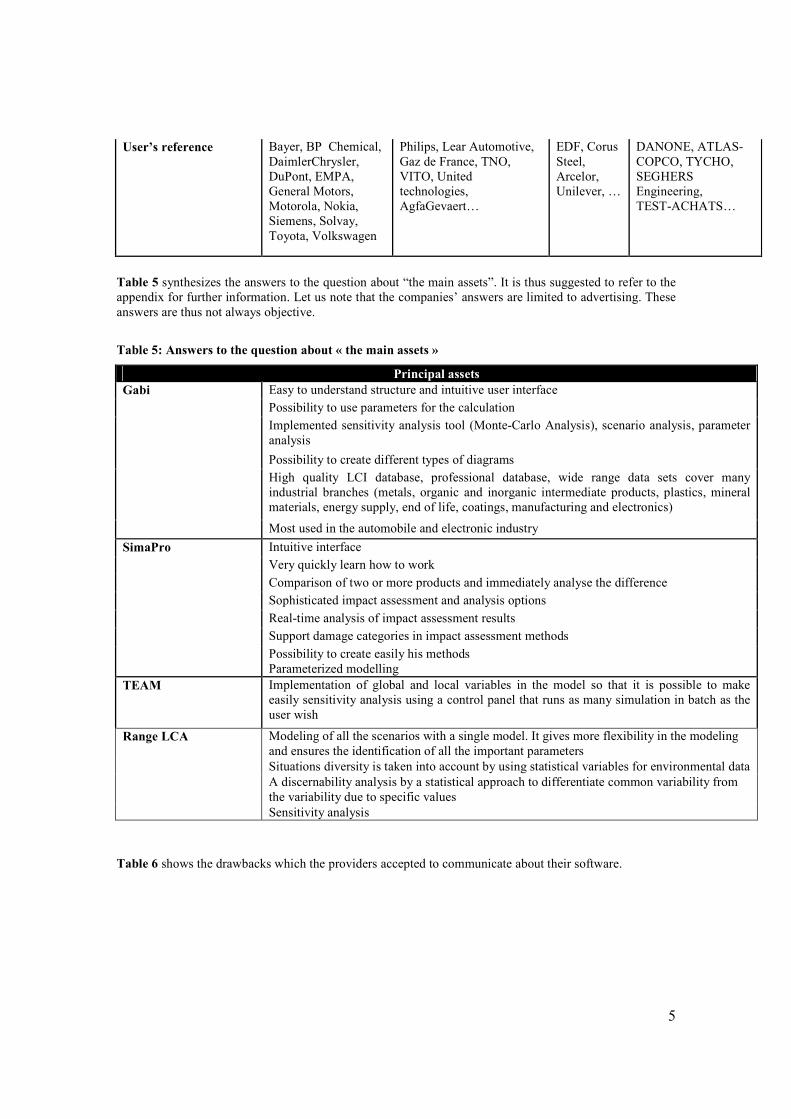
5

User’s reference Bayer, BP Chemical,

DaimlerChrysler,

DuPont, EMPA,

General Motors,

Motorola, Nokia,

Siemens, Solvay,

Toyota, Volkswagen

Philips, Lear Automotive,

Gaz de France, TNO,

VITO, United

technologies,

AgfaGevaert…

EDF, Corus

Steel,

Arcelor,

Unilever, …

DANONE, ATLAS-

COPCO, TYCHO,

SEGHERS

Engineering,

TEST-ACHATS…

Table 5 synthesizes the answers to the question about “the main assets”. It is thus suggested to refer to the

appendix for further information. Let us note that the companies’ answers are limited to advertising. These

answers are thus not always objective.

Table 5: Answers to the question about « the main assets »

Principal assets

Gabi Easy to understand structure and intuitive user interface

Possibility to use parameters for the calculation

Implemented sensitivity analysis tool (Monte-Carlo Analysis), scenario analysis, parameter

analysis

Possibility to create different types of diagrams

High quality LCI database, professional database, wide range data sets cover many

industrial branches (metals, organic and inorganic intermediate products, plastics, mineral

materials, energy supply, end of life, coatings, manufacturing and electronics)

Most used in the automobile and electronic industry

SimaPro Intuitive interface

Very quickly learn how to work

Comparison of two or more products and immediately analyse the difference

Sophisticated impact assessment and analysis options

Real-time analysis of impact assessment results

Support damage categories in impact assessment methods

Possibility to create easily his methods

Parameterized modelling

TEAM Implementation of global and local variables in the model so that it is possible to make

easily sensitivity analysis using a control panel that runs as many simulation in batch as the

user wish

Range LCA Modeling of all the scenarios with a single model. It gives more flexibility in the modeling

and ensures the identification of all the important parameters

Situations diversity is taken into account by using statistical variables for environmental data

A discernability analysis by a statistical approach to differentiate common variability from

the variability due to specific values

Sensitivity analysis

Table 6 shows the drawbacks which the providers accepted to communicate about their software.

6

Table 6: Answers to the question about « the drawbacks» (nc: not communicated)

Drawbacks

Gabi multi user capability of the software not available

SimaPro scenario analysis not supported

TEAM nc

RangeLCA nc

The cost of the various software tools shows strong differences between the purchase of an academic

license “university” (education, small-scale research project) and a professional license (consulting

companies, large-scale research project, etc.)

For SimaPro, an academic license for one year and one user costs 900 € for the PhD version and 1800 euros

for the faculty version. The classroom version (40 users client version) costs 1500 € per year. Educational

versions may only be used by academic institutes for teaching purposes and cannot be used for commercial

activities or paid research.

A One year license for one user costs 5300 € for TEAM. The cost for the same product is intermediate for

Gabi. A Four years license including updates and service costs 10000 € for RangeLCA.

The prices are also very different for the professional license. For one user and one year of service, the least

expensive remains SimaPro with 4800 € (developer version), followed by Gabi with 7 500 €. The cost for

one professional license for TEAM and for the service is 10 000 € per year! For TEAM, the prices for two

licenses haven’t been asked because of the high price of one license.

After consultations with the providers, the license necessary for our study is a professional one.

Table 7: License cost estimation (2007)

Estimation (taxes not included)


Academic license 3750€ 900€(PhD),

1500€ (classroom,)

2000 €

1800€(Faculty)

Additional license Free nc 1000 €

Service Free Free the first year 2300 €

(contract

maintenance)

400€ (single user)

800€ (multi user) Free

Professional license 7500€ 1800€ (compact),

3000€ (analyst)

10000 €

(consultant)

4800€ (Developer) per year 10 000 €/ 4 years

Additional license Free 1800€ nc

Service Free Free the first year Included (first

year)

1200€ (1800 € for 2 and

600€ for each extra user)

Free

From the results of the questionnaire, it appears that the four software tools show many similarities but

they also comprise some specific characteristics. The major differences are the possibility to carry out other

types of analyses than environmental ones, the type of file for import and export and the cost of the

software tools.

As a conclusion, at this stage, it is difficult to select an LCA software on the basis of the answers to the

questionnaire only. The test of the software’s demonstration versions and the comments must allow to

determine the most adequate software and to improve judgement.

7

3.3. Demonstrations

Besides the questionnaire, the selection of the software has been based on the test of the software

demonstration versions. The comparison is not easy since each demonstration software possesses its own

characteristics.

Some demonstrations, like Gabi and SimaPro, propose to conceive an LCA following a specific tutorial.

The software’s demonstration provided by SimaPro presents a complete study of a simple wooden shed

(time of the realisation: more than two hours) and an exploration of an example of LCA. The Gabi’s demo

on the other hand is much briefer (time of using is approximately 20 minutes).However The TEAM

software’s demonstration doesn’t allow undertaking an LCA. It only shows the stages of an LCA’s

realisation.

As RangeLCA is developed for internal use; it doesn’t have a demonstration version. We made a trial with

the complete software.

Thus, no unbiased comparison could emerge from the use of the three demonstrations tests. Moreover, any

comparison starting from a random and easy LCA, imagined at the ETEC department, could not be

realised. Indeed, each demonstration exercise has specific limitations of use.

In spite of these restrictions, some comments can be proposed. They can sometimes refute the answers to

the question related to the “principal assets” (see table 5).

3.3.1. Gabi

• no intuitive use

• good visibility of the process tree

• lack of visibility in the fitting of the running windows

• no modification existence in the event of error in the architecture of the processes?

3.3.2. SimaPro

• intuitive use

• good visibility of the fitting of the running windows


• construction of the software seems rigid

3.3.3. TEAM

• intuitive use



• seems to have an important series of tools for the study

3.3.4. RangeLCA

• intuitive use



• very good statistical skills

• high reliability of the outcomes

• recognition of the diversity of the individual cases

• automatic sensitivity analysis of all the parameters

8

From this test, the selection focuses on three software tools: SimaPro, TEAM and RangeLCA.

4. Conclusion

The selection of the LCA software is not easy to achieve. After a preselection, four software tools

(SimaPro, TEAM, Gabi and RangeLCA) were held and analyzed on the basis of the responses to the

questionnaires, as well as on the demonstration version tests proposed by the companies.

After the preselection, RangeLCA seems to be the most adequate software for this study. Indeed,

RangeLCA has innovating characteristics and many assets, compared to other LCA softwares. The

outcomes show the diversity of the individual cases and integrate automatically the sensitivity analysis of

the parameters. Its produced results integrate a set of possible combinations for the various parameters and

data in order to take into account possible synergy and compensation effects. However, it is important to

note that Gabi has interesting references in the automotive industry (Daimler Chrysler, General motors and

Toyota) but it was eliminated due to the lack of user-friendliness. TEAM also has interesting features .but

they are less appropriate for the project.

Cost estimation was requested at Price Waterhouse Coopers-Ecobilan for TEAM, at PRé Consultants for

SimaPro and at RDC-Environment for RangeLCA.

Table 8: Final cost estimation of the softwares (na: not asked; include a one day in-house training for

the CLEVER project, travel costs not included).

Cost estimation (tax not included)

SimaPro TEAM RangeLCA

Professional License (1

user) + database

4800€ 10000€ 10000€/4 years

Service (one year) included included Included

Ecoinvent database Included 1200€ 1200€

One day in house

training

5000€ 1160€ free€

Total for 1 license 9800€ 12360€ * 11200€/4 years

After the comparison of the main assets of the three software packages and after cost consideration,

RangeLCA remains the most adequate software. RangeLCA includes a powerful statistical tool which

allows taking the diversity of all the analysed situations into account. Moreover as the duration of the

project will be 4 years, RangeLCA has the lowest license and service costs, and the location of the

company makes interactions much easier during the course of the project.

9

Appendix: Questionnaire

10

1. Overview

The appendix contains the responses to the questionnaire sent to the LCA software developers. The

questions asked to them include the after-sales services provided (online and phone support, training), the

software functionality and the databases quality (the Content, the Updating options, European and

international validity). A few examples of organizations using the different software packages and having

performed LCA studies similar to ours with the software the different software packages were also asked to

the program developers.

2. Supported

2.1. Supported, updated The question: Does the software provider offer after sales services (e-mail support, hotline service, and

update)?

2.1.1. Gabi 4

Software updates are released if required and are free of charge. Updates can be downloaded from our

website. Naturally the Gabi software is prepared for all future updates of process data and impact

assessment data.

2.1.2. SimaPro 7

Software and database updates are included in the service contract; this also applies to new versions. A free

first year service contract is included in indefinite licenses.

At the beginning of the summer a new version is expected to be released.

2.1.3. TEAM 4.0

Yes, if the customer subscribes to the maintenance contract (2300 euros). The contract includes 8 hours hot

line and updates (if any) for one year.

2.1.4. RangeLCA 2.1

Software update and service are included in the license contract.

2.2. Service hotline

2.2.1. Gabi 4

As a Gabi customer you have free access to email and hotline support from PE Europe. No additional fee

has to be paid.

2.2.2. SimaPro 7

Hotline, e-mail, phone and fax support are included in the service contract.

11

2.2.3. TEAM 4.0 See 2.1.3

2.2.4. RangeLCA 2. Included in the license contract.

2.3. The training The question: “Do you propose a training (via seminar or personalised)? What would be the cost of the

training? Are the trainings being organized on a regular base? Weekly? Monthly? Yearly? What is the

maximal waiting period between the training(s)?”

2.3.1. Gabi 4

We offer our customers training on site as well as training sessions at PE Europe. The price is depending on

the content of the training within the range of 400€ for one day training to 1100€ for a 2 days expert

training at PE Europe.

Training sessions at the customer’s office are charged with 900€ per day excluding expenses. The content

of an on site training is variable from introduction courses to personalized training sessions regarding

specific questions.

2.3.2. SimaPro 7

PRé Consultants can organize in-company trainings. A major benefit of the in-company training is the

freedom to modify the content of the training to meet your individual needs.

Customization allows you the flexibility to emphasize the most relevant issues and to minimize those not as

relevant. It is an excellent occasion for the persons involved to share the same knowledge at the same time.

The kick-off of a LCA program might be a good example.

The fee for a one day in-house training is 5000 Euro. For two or three days the fee will be 8000 Euro or

10.000 Euro respectively.

This fee includes a review of one LCA study (taking maximum 8 hours of our consulting staff). Travel

costs and VAT (where applicable) are not included.

We assume the in-company training will be attended by 5 people maximum.

We organize regular training courses in Amsterdam, about every 3-4 months, dependent also on the

interest. The next training is scheduled at the end of May (2007) Personalized courses can be arranged but

are more expensive.

a. Topics

The training will contain the following elements:

- Introduction in LCA terminology: what is goal and scope, system boundary, allocation etc?

- Structure of SimaPro: libraries and projects.

- Modelling in SimaPro: processes and product stages, waste scenarios.

- Documentation.

- Backgrounds of inventory data and methods in SimaPro.

- Introduction in inventory (data collection).

- How to analyze results.

- Using Wizards.

- Data management: import/export, append substance names.

- LCA in practice, including your own specific questions.

Further we will give a preview of new SimaPro features you can expect soon.

12

b. Trainers

The training will be given by two of our experienced consultants, who have done numerous LCA projects

and use SimaPro on a daily basis.

c. Optional LCA support and review package

We offer an optional follow-up module where we provide you with 8 hours extended support and reviews

of your LCA project within a 6 month period.

d. Date and Location

The next training day is Wednesday 9 May 2007. The location of the course is the NH Barbizon Palace, in

the center of Amsterdam opposite Central Station.

e. Prerequisites

The attendees need a basic understanding of LCA and the operation of Windows software. Further they are

expected to have read the SimaPro demo manual as well as part of the SimaPro user manual.

f. Conditions

All training sessions and documentation are in English.

The maximum number of participants for each training is 10. If the course is fully booked you can be put

on a waiting list.

PRé Consultants reserves the right to make changes in the program, date, location and trainers or to cancel

the training if enrolment criteria are not met or when conditions beyond its control prevail. In such cases,

every effort will be made to contact each trainee and an alternative will be offered. If training is cancelled

for any reason, PRé Consultants is limited to refund the training fee only.

g. Next training

Date: Monday/Tuesday May 24-25, 2007.

Location: NH Barbizon Palace in the centre of Amsterdam, opposite Central Station.

Costs:

- 1500 Euro for 2 days training, including lunch and evening event, excluding VAT, travel.

arrangements and insurance.

- 1200 Euro for optional LCA review package.

2.3.3. TEAM 4.0

Tutorials are organised on customers demand. There is no waiting period except if no engineer is available

at the time.

2.3.4. RangeLCA 2.1

Trainings are organised when e-mail and telephone supports can’t solve the problem. It is included in the

license contract. Trainings are organised in the week on the demand of customers unless the engineers are

not available.

3. Functionality

3.1. Minimal requirements The question: “Is the software compatible with PC and which are the capacities required of our computer

(processor, RAM...)?”

3.1.1. Gabi 4

13

The system requirements of Gabi are: PC with at least 400 MHz, 128 MB RAM, 100 MB free hard disk

space (the actual hard disk storage depends on the size of the databases created).

3.1.2. SimaPro 7

SimaPro is developed to run optimally on Windows PC's with a Pentium 4 processor.

You may run SimaPro on a Macintosh/Unix computer using Windows emulation software. We regret that

however we cannot give technical support for these systems.

Processor

Minimum requirement: Pentium III or equivalent. For optimal performance we recommend Pentium 4

(equivalent) 2.0 GHz or better.

Internal memory

The table below shows the minimum and recommended memory requirements for the operating system

plus SimaPro.

Operating system Recommended (MB RAM)

Windows 2003 server 512

Windows XP 512

Windows 2000 512

Windows NT 4 256

Windows ME 256

Windows 98 256

If you use other software applications simultaneously with SimaPro, add the required memory for these

applications.

Hard disk

A minimum of 1 GB of free hard disk space is required. For larger databases you will need more space.

Monitor

SimaPro can be run at a resolution of 800 x 600. A higher resolution is recommended.

CD-ROM

A CD-ROM drive is needed to install the software. No installation on diskettes is available. As alternative

you may download and register the full demo version to install as a single user.

Internet

An internet connection is needed to check for availability of software and database updates on-line. See in

the SimaPro menu bar under Help, Check for update.

3.1.3. TEAM 4.0

The software is compatible with PC (memory: minimum 64 MB of RAM, recommended 128 MB or more,

processor: Pentium class processor).

14

2.1.4 RangeLCA 2.1

Technical requirements of the software:

Minimum P III 800 MHz, PIV 2GHz is recommended

Minimum 128 MB RAM, 512 to 1024 MB are recommended

20 GB of hard disk (included database)

3.2. Microsoft Windows operation system The question: “Intend to work under Microsoft Windows operation system?”

3.2.1. Gabi 4

Gabi 4 is a 32-bit application that was developed for Windows95™, Windows.NET™, Windows2000™

and Windows™.

3.2.2. SimaPro 7

SimaPro 7 is a 32-bit Windows application which runs under Windows 98, Windows ME, Windows NT

4.0, Windows 2000, Windows XP and Windows 2003 server. It is recommended to have the latest service

packs installed.

Under certain circumstances the Administrator right may be required for installation under Windows 2000,

XP, and 2003 server.

Multi-user version

The multi-user version runs as a client-server system over TCP/IP networks. The SimaPro Server must be

installed on a computer with a Windows operating system, Novell servers are not supported.

Multi-user installation should be done by your system administrator/IT department.

3.2.3. TEAM 4.0

Yes

3.2.4. RangeLCA 2.1

Range LCA runs under Windows 98, 2000, Millennium and XP.

3.3. The size and the complexity of the process model The question: “Is the process model unlimited in size and complexity?”

3.3.1. Gabi 4

Yes, within Gabi you can model systems with a huge number of sub-systems and used processes. One of

our biggest systems is built up out of more than 25.000 plans containing about 300.000 processes and is

still easy to understand due to the Gabi structure.

3.3.2. SimaPro 7

Yes, note that non-linear functions are not supported.

15

3.3.3. TEAM 4.0

The maximum size of the database depends of your machine capacity. We work on large-size databases

(for more detail contact Anis Ghoumidh) and have no problem. There is no limit to the complexity of the

database (from our experience). The tool is intended for life cycle assessment and is compatible with ISO

14040-41-42-43 standards.

2.3.4 RangeLCA 2.1

There is no size limit for system modelling. Models of 400 processes have already been performed.

3.4. Inventory and impact assessment The question: “Does the software support inventory and impact assessment?”

3.4.1. Gabi 4

Yes, Gabi supports inventory as well as impact assessment.

3.4.2. SimaPro 7

Yes

3.4.3. TEAM 4.0

Yes, the tool supports inventory and impact assessments.

3.4.4. RangeLCA 2.1

Yes

3.5. Graphical interface

3.5.1. Gabi 4

Processes are arranged in Sankey diagrams, allowing a quick overview of mass, energy or even cost flows

shown as proportional to quantity. It is up to the user to determine which additional flow quantities one

wishes to depict in this sophisticated manner. Furthermore the process names and quantities can be

displayed. The display of user defined process images makes the presentation and the understanding of

complex processes easier.

3.5.2. SimaPro 7

From the graphics (results) you can get to the editors, but we do not have a graphical editor. As the models

we work with can get very complicated, a graphical interface does not make much sense. However the

system as it is implemented will give you full access to all you could need and works as good as a graphical

editor. If you need further explanation let me know.

3.5.3. TEAM 4.0

16

Yes

3.5.4. RangeLCA 2.1 Yes

3.6. Import and export possibilities (from/to MS Office tools? Others?)

The question: Is it possible to import and export data from/to MS Office tools? Others.

3.6.1. Gabi 4

Export to Excel:

Exporting Gabi processes to Excel is completed just as simply and quickly as importing. With the simple

copy and paste function, such as known from Microsoft, you can copy a Gabi process in an Excel table

sheet. Further you have the possibility to drag & drop any kind of database object (balances, plans,

processes, flows, quantities or whole projects) from one Gabi 4 database to another via the Drag-and Drop-

functionality

Import from Excel:

To be able to import processes from MS Excel, the table format can be adapted to the requirements of Gabi.

Hence the import of data from Excel is very easy. The export and import to/from Excel is also possible to

other Gabi objects, such as flows and balances for example.

3.6.2. SimaPro 7

Import via CSV, Spold99, ECOSpold (soon) and SimaPro database format. CSV file can be created via

Excel. Export to CSV, txt, XLS, Spold99, SimaPro database format and various graphical formats for

graphs. Copy and paste of results to Office applications is fully supported.

3.6.3. TEAM 4.0

Yes via txt files (TEAM format and SPOLD format), import of any Ecoinvent 2000 formatted data. From

MS office, copy and cut, and save (as Excel format) are available.

3.6.4. RangeLCA 2.1

Yes Import/export via excel files. Import/export via XML files option will be available in the summer of

2007.

3.7. Possibility to change impact factors

3.7.1. Gabi 4

Gabi 4 allows users to create individual performance indicators for the evaluation of the systems. Impacts

of substances with respect to internationally discussed impact categories such as global warming potential,

acidification potential, toxicity potentials, ozone depletion potential and more comply with

recommendations of ISO, SETAC, WMO and IPCC. These features provide quick and transparent

17

evaluation of the environmental, technical, economic or social performance of your plants, processes,

services or products.

Changing impact factor view on results:

In Gabi it is very easy to switch between mass or energy balance and even impact results or one-point

indicators. You can change the displayed impact factors within a Gabi balance with just one click.

Edit impact factors:

The open structure of Gabi gives you a maximum freedom of changing, creating and deleting all kinds of

objects used in Gabi.

If you want to add flows to an impact factor or delete flows, create your own impact factor.

3.7.2. SimaPro 7

Yes.

3.7.3. TEAM 4.0

Yes.

3.7.4. RangeLCA 2.1

Yes it is possible to change impact and normalization factors. For the moment it is done by RDC-

Environment on customer’s demand.

3.8. Possibility to change weighting factors

3.8.1. Gabi 4

You can change the displayed impact factors within a Gabi balance with just one click.

3.8.2. SimaPro 7

Yes. Our impact assessment methods are fully flexible. You can also copy a method and change it, or

create your own methods. SimaPro is the only tool to support damage assessment.

3.8.3. TEAM 4.0

You can change the reference flow and the reference value for the functional unit. Normalisation methods

can be created and applied but do not exist as such.

3.8.4. RangeLCA 2.1

Yes, see 2.7.4.

3.9. Possibility to change reference value (normalisation)

3.9.1. Gabi 4

18

As easy as the change of weighting factors, you can apply different normalisations to your results with one

click. As a matter of fact, it is also possible to edit these normalisation factors as explained for the impact

factors.

3.9.2. SimaPro 7

Yes.

3.9.3. TEAM 4.0

If it is for normalisation, see 2.8.3.

2.9.4 RangeLCA 2.1

Yes see 2.7.4

3.10. The speed of calculation

3.10.1. Gabi 4

If you work with a computer fitting to the system requirements, Gabi is able to handle very huge systems at

a very comfortable calculation time.

We run some calculations to test the performance of Gabi:

A computer running Win XP, with 2.4 GHz and 512 MB needs only 32 seconds (!) to calculate a balance

out of 19.500 systems and 310.000 processes. A system with 7.000 plans and 115.000 processes needs

approximately 17 seconds, and a smaller system with 16 plans and 330 processes need about 1 second to

calculate a balance.

Within a Gabi balance you can do several kinds of analysis. For example applying a parameter variation

within a Monte-Carlo analysis of a medium sized system structure of about 100 modelled processes takes

in a Monte-Carlo simulation (1000 simulation runs) about 60 seconds to calculate all possible impact

systems.

3.10.2. SimaPro 7

This cannot be answered as it is not only dependent on the PC configuration but also on the model you are

analysing.

3.10.3. TEAM 4.0

It depends on the machine.

2.10.4 RangeLCA 2.1

One of RangeLCA’s main assets is its calculation speed. To calculate 300 processes, Range LCA will need

45 seconds and that for 1000 calculation iterations.

Better calculation speeds are expected with Intel Core 2 Duo processor and high speed RAM (667 MHz

and more).

19

3.11. Time to master the software

3.11.1. Gabi 4

This depends on the complexity of the models you want to analyze. For a non complex modelled system it

is possible to get results after the first day. Hence the complexity of modelling in Gabi can be increased to a

maximum level of detail, if the problem you want to solve requires so. Developing complex process models

Gabi provides several modelling possibilities which need some experience in the work with Gabi. Due to

the complexity of the modelling, your experience will increase and Gabi will never set any border to the

possibility of modelling.

3.11.2. SimaPro 7

2-5 Days. We offer a tutorial to learn the basics of the operation of SimaPro. See 1.3.1.

3.11.3. TEAM 4.0

Two days to one week.

3.11.4. RangeLCA 2.1

3 days to one week.

3.12. Other types of analysis (costs, socio-economic impacts...)

3.12.1. Gabi 4

Cost Considerations:

Gabi4 enables consideration of different cost factors connected to the processes or the lifecycle of products.

Users are supported by advanced wizards when keying in various cost types. Gabi 4 then automatically

computes costs related to individual processes, material or energy flows from the user’s details.

Social Conditions:

The quality of work environment can be computed and evaluated along the value chains by newly

developed features.

3.12.2. SimaPro 7

No, if you are looking for predefined methods and a ready made setup. Yes, if you are prepared to put some

effort in defining the methods to do so. Note we are working on these issues.

3.12.3. TEAM 4.0

Cost analysis can be carried out if costs data are available. TEAM takes into account both fixed and

variable costs.


20

Since 2004, RDC-Environment is working on Impact monetarisation.

3.13. User-friendliness

3.13.1. Gabi 4

The user-friendly Windows interface of the Gabi 4 system makes it easier to handle thanks to the flexible

and graphical user screen windows. The multiple windows technology provides you with flexibility,

allowing you to have your own individual working style. Clear dialog boxes, drag & drop technology and

the use of symbols improve one’s ability to operate the system in terms of software ergonomics.

The structure of Gabi is geared towards the use of the functionality of the Windows™ Explorer. So the user

will be very familiar with the usage of the Gabi software.

3.13.2. SimaPro 7

A hint: in SimaPro you need only a few mouse clicks to define a flow, and it is very easy to analyse the

results in detail. Further we have an LCA Wizard that will help you modelling (see the guided tour in our

demo).

3.13.3. TEAM 4.0

Many customer say yes. Other thinks it is a bit complicated (as life cycle assessment is!)


Range LCA is developed for internal use, so there is no users guide or manual. Modelling on Range LCA is

done by process tree, which makes it user-friendly. The fact that you can model several systems in one

model avoids you to repeat the modelling of common parts.

4. Database

4.1. The data collection

The question: “Does the database contain data on raw materials, power generation, transport and

disposal?”

4.1.1. Gabi 4

The Gabi database have a clear and comprehensible structure and can be extended easily by the user.

Metals, plastics, energy carriers, auxiliary substances, transport processes, chemical intermediates, mineral

substances, building materials, parts and papers, etc. may not be everything, but in comparison with

competitors, they offer a convincingly high coverage off the most important fields and a high level of data

quality – this makes up the difference.

GaBi 4 Professional database includes approx. 650 sets of data (cradle to gate), generated by IKP/PE. This

data is based on information from patent/specialist literature and industry which makes GaBi 4 to one of the

leading databases in the world. These data sets include the decisive areas of the pre-chains to metals (steel,

aluminium and non-ferrous metals), organic and non-organic pre-products, synthetics, mineral materials,

provision of energy (steam, thermal energy, electricity mixes and power stations), end of life and disposal

and processing with.

Nevertheless, specific data demand may exist. Your own inquiries are often time consuming and therewith

21

quite expensive. PE Europe can provide you with individual customized data on demand, either from our

stock or individually generated.

4.1.2. SimaPro 7

• ETH-ESU 96

Focus: Energy. Electricity generation and related processes like transport, processing, waste treatment.

Includes 1200 unit processes and 1200 system (results) processes. Extensive documentation provided.

Source: ETH-ESU. Licensed database.

Availability: Included in standard database (commercial and educational versions).

• Dutch Input-Output database

Focus: Economic Input-Output database, for us on its own or in hybrid LCA studies.

Starting point was an overview of how the average consumer distributes its spending over 350 categories,

such as buying tomatoes, driving to work and maintaining the garden. A link was made between these

categories and the economic sectors. The economic input output table was used to trace the trade flows

between these sectors.

We also introduced foreign input-output tables for the OECD and non-OECD regions. This allows us to

actually trace the impact of goods produced outside the Netherlands.

Source: own data collection, as part of a project


• BUWAL 250 database

Focus: Packaging materials (plastic, carton, paper, glass, tin plated steel and aluminium), energy, transport,

waste treatments.

Source: BUWAL 250, 2nd edition. Fully documented and licensed database.


• INDUSTRY DATA

Focus: Inventory data provided by industry associations. Mostly cradle to grave data.

Source: various, APME.


• IDEMAT 2001 database

Focus: Engineering materials (metals, alloys, plastics, wood), energy and transport.

Source: Data collection from various sources supervised by Dr. Han Remmerswaal, Faculty of Industrial

Design Engineering, Delft Technical University, The Netherlands.


• FRANKLIN US LCI database

Focus: North-American inventory data for energy, transport, steel, plastics, processing.

Source: Data collected by Franklin Associates, USA. Fully documented and licensed database.

Availability: Included in commercial versions. Must be purchased separately for educational versions.

• Data archive

Focus: Materials, energy, transport, processing, waste treatment.

Source: Variety of older public sources (PWMI, BUWAL 132, ETH, SPIN, Chalmers, Kemna).


• Dutch Concrete database and scripts

Focus: Dutch data related to all aspects of concrete production and use. Can be used in combination with

scripts. Data and scripts are in Dutch.

Source: Betonplatform, the Netherlands.

22

Availability: Free for Dutch users with service contract. Available on request for other customers with

service contract, however no language support is given. This database is protected against copying and

export.

• IVAM 4.0 database

Focus: Materials, transport, energy and waste treatments. Mostly focused on Dutch data.

Source: Data collected by IVAM Environmental Research, Amsterdam, the Netherlands. Also

ETH/BUWAL and PRé data included.

Availability: Purchase from IVAM Environmental Research. The price is 1575 Euro, excluding VAT.

• FEFCO database and scripts

Focus: European data on corrugated board production, partially based on BUWAL 250. Includes scripts to

model the production and life cycle of corrugated board.

Source: FEFCO, European Association of Corrugated Board Manufacturers, Belgium.

Availability: Only together with SimaPro Light license through FEFCO. The accompanying report is

available free of charge.

• Eco-invent data

The ecoinvent 2000 database is an up-to-date, consistent dataset of 2500+ generic processes for the Swiss

and Western European area. With the release of this database by the Swiss Centre for Life Cycle

Inventories, a major update for the BUWAL 250 and ETH-ESU 96 databases has been delivered.

PRé Consultants recognizes the value of this database and had become reseller of ecoinvent licenses.

Currently we are making the database available in SimaPro format.

The ecoinvent 2000 database covers a broad range of processes in the following sectors:

- Energy

- Transportation

- Waste Management

- Building Materials

- Chemicals

- Washing agents

- Paper & board

- Agriculture

4.1.3. TEAM 4.0

Yes. Basic data are available in the TEAM package. Specific ones can be ordered.

4.1.4. RangeLCA 2.1

Yes. RDC-Environment developed its own database based on the different LCA projects they have

performed. They continue to develop this database with the results of their new projects. It is recommended

to buy the Ecoinvent Database for RangeLCA.

4.2. Up-to-date

4.2.1. Gabi 4

The professional database is based on the years 2002 to 2004. The new land use databases, released in

spring 2007, will be delivered free of charge to all current Gabi users and will be an integral part of the

standard Gabi package for new users.

4.2.2. SimaPro 7

23

The ecoinvent V2 version will be available in the summer of 2007.

4.2.3. TEAM 4.0

We depend on public data and project availability

4.2.4. RangeLCA 2.1

The RangeLCA database is under development.

4.3. European and International validity? The question: Do the data contained in the databases have an European and International validity?

4.3.1. Gabi 4

• The database documentation format conforms to the ELCD (European Reference Life Cycle Data system)

standards and all documentation is now based on the standards defined for European LCI database.

60 additional country specific power grid mix modules and the possibility to set up individual power grid

mixes make GaBi 4 the most comprehensive LCA database on energy systems world-wide.

• All 110 ELCD data sets of the first European LCI database are included. The basis of these data is

information from the participating industry (EAA, ECI, EUROFER, FEFCO and PlasticsEurope) and

PE/LBP background data. PE International, LBP (University of Stuttgart) and other their partners enjoyed

the confidence of the EU Commission in being chosen to set up of the first European LCI database.

4.3.2. SimaPro 7

Yes

4.3.3. TEAM 4.0

Most data are valid for Europe as most data are published in Europe.

4.3.4. RangeLCA 2.1

Yes

4.4. Adjustable

4.4.1. Gabi 4

All datasets using parameters are free for new settings entered by the user. As a matter of that any database

object can be edited by the user.

4.4.2. SimaPro 7

Yes

24

4.4.3. TEAM 4.0

Yes, a module can be copied and pasted and the copy can be modified.

4.4.4. ‘RangeLCA 2.1

Yes, a process can be removed from the database and it can be modified afterwards.

5. Similar LCA

The question: “Has this software been used by a similar LCA study as ours?”

5.1. Gabi 4 The Gabi software was especially designed for the use of LCA studies. Therefore Gabi has been used for

LCA studies of all kinds of products (also vehicles) during the last 10 years.

5.2. SimaPro 7 We do not keep track of SimaPro by our users, often studies are confidential.

5.3. TEAM 4.0 Yes we modelled the life cycle of a vehicle, electronics equipment, eco-design etc.

5.4. RangeLCA 2.1

Yes, but only for the using phase of a vehicle

6. Organizations using the software?

The question: “Could you provide us with a few examples of some organisations using your software?”

6.1. Gabi 4

Clients come from all branches with a focus on materials, chemical, energy, automobile and electronics

industry, e.g. Alcan, Asahi Kasei, Bayer, BP Chemical, DaimlerChrysler, DuPont, EMPA, General Motors,

Motorola, Nokia, Rio Tinto, Siemens, Solvay, Sydney Waters, Toyota, Volkswagen, etc.

Universities using Gabi: Ecole Polytechnique de Montreal, Universität Jena, Norwegian University of

Science and Technology, Forschungszentrum Karlsruhe, RWTH Aachen, Universität Wien, Deakin

University, Tokyo University, National Taipei University etc.

6.2. SimaPro 7 Philips, Lear Automotive, VITO Belgium, AkzoNobel, Sara Lee, United Technologies, Gaz de France,

TNO, TU Delft, AgfaGevaert, Heineken, FEFCO, Pfizer and various universities in Belgium.

25

6.3. TEAM 4.0 EDF, Corus-Steel, Arcelor, some construction products manufacturers, FAT (Research project),

Unilever...etc.

6.4. RangeLCA 2.1 RangeLCA is used by RDC-Environment engineers.LCA of air compressors, LCA study on Raychem &

competitive telephone splice closures, Comparative LCA of different elimination options of sewage sludge,

LCA of consumable goods (Passenger car, white goods, Household detergent and packaging) and

development of a formula for calculating the environmental performance of these products are LCA

projects performed by RDC-Environment.

7. Reference tool

The question: “Is your software widely accepted as a reference tool?”

7.1. Gabi 4

As you can see in the reference list above, many leaders of different branches use Gabi as their standard

LCA tool.

7.2. SimaPro 7 They have hundreds of users in more than 45 countries, making SimaPro the most widely used LCA

software.

7.3. TEAM 4.0

Not communicated

7.4. RangeLCA 2.1 RangeLCA has been used to perform some studies for several Belgian and international companies.

8. The main assets of the software compared with the other

softwares found on the market (TEAM, Gabi 4, SimaPro 5

and RangeLCA 2.1)?

8.1. Gabi 4

Gabi is a comprehensive tool. Due to the easy to understand structure and intuitive user interface, very

complex and individual modelling is possible. One more time the comparison with the car you can quickly

and easily learn how to drive a car, but understanding the complex structure and the background needs

some time.

Parameters:

Compared to other available LCA tools one of the unique selling points is the possibility to use parameters

for your calculation. Parameterised process models allow the definition of non-linear equations (e.g. non-

26

linear input-output relations) which are the basis for parameter variation and scenario balances. Therefore

the set-up of one parameterized process can simulate thousands of different process characteristics (e.g.

different operation modes etc.) The Gabi 4 Analyst facilitates this. Other new analysis features

implemented in Gabi 4 are the Sensitivity Analysis and the user-friendly and Monte-Carlo Analysis.

Gabi 4 is the only software available on the market that can handle parameters.

Handling:

Gabi supports you with a lot of useful tools e.g. the consistency check helps to minimize systematic error

possibilities.

Within the weak point analysis you can highlight or hide values that differ an entered percentage.

Presentation of results:

Several new easy-to-use balance-exploring functions and flexible filters for categories like "country" or the

weak-point analysis helps you to analyze your results without the need of entering complicated settings.

In Gabi you can create different types of diagrams (bar, column, pie, scatter point or line charts) from each

balance view. The charts relate to the current representation in the input or the output table, which is, by

means of an appropriate switch of the balance view you can create diagrams of inventories, normalised

balances or evaluated balances. The diagrams are created separately from the input and the output table.

The diagrams can be transposed and stacked. The user has a lot of possibilities to customise the diagram.

Furthermore the diagram can be copied into several Microsoft applications like Word and PowerPoint.

Like in Excel it is possible to mark an area in the balance and create a diagram out of it.

Database:

A further unique selling point is the high quality LCI database delivered with the software. The standard

database delivered with the Gabi 4 software is the professional database. This database contains 638

processes out of different branches and is an optimal basis to apply LCA.

Furthermore twelve extension databases are available for the Gabi 4 software. The wide range of the Gabi 4

data sets cover many industrial branches including metals (steel, aluminium and non-ferrous metals),

organic and inorganic intermediate products, plastics, mineral materials, energy supply (steam, thermal

energy, power grid mixes), end-of-life, coatings, manufacturing and electronics.

We are an official re-seller of the Swiss ecoinvent database which contains more than 2500 processes from

different sectors including energy supply, building materials and building processes, chemicals, detergent

ingredients, graphic papers, transport, disposal, agricultural products and processes. Purchasing the

ecoinvent database includes a license of ecoinvent allowing full access to the ecoinvent download website.

8.2. SimaPro 7 -LCI model in SimaPro

In SimaPro, creating a model is easy compared to many competitors, due to the intuitive user interface.

Linking a process with another process or a substance can be done with a few clicks, whereas in other

software tools you need to follow a rather complex procedure. As a result, new users very quickly learn

how to work in SimaPro. To further improve the learning curve, we offer extensive documentation

including a User Manual and Tutorial (you can find these via Help in the menu of your SimaPro demo).

We also support advanced modelling for the assembly and disposal of complex products, via the product

stages. This allows you to assign different product parts (assemblies) of product to different waste streams

(disposal scenarios), with semi-automatic modelling of the waste treatments of the individual materials

used in your product model. This will save you the time assigning each material to an individual waste

treatment.

Furthermore we offer LCA wizards to help you start building your model in SimaPro, in the demo these

can be found in the automatic Guided Tour script.

Indeed SimaPro does not support variables. Apart from practical and technical reasons, we feel that one

needs to analyze the differences between different products, and analyzing a product one by one with

different variables does not give you the desired comparison in one convenient overview. In SimaPro you

can compare two or more products and immediately analyse the differences.

27

To make sure you can quickly adjust your model, we implemented various copy options for individual

processes and partial or full models.

-Analysis of models in SimaPro

Generic model analysis is easily done in SimaPro using the process tree or network. Here you have the

option to show various material or substance flows, use a cut-off to hide less important processes. Various

navigation, find, and analysis options are given.

In the new SimaPro we will implement Monte-Carlo analysis. This works optimally in combination with

the new ecoinvent database (www.pre.nl/ecoinvent) where uncertainty data are available in the Unit

processes. We will support both analysis of a single model or a comparison of 2 models (with process

coupling to make sure that processes that are used in both models are varied in the same way) and detailed

graphs and tables will be available. Scenario analysis is not supported.

-Impact assessment in SimaPro

SimaPro is well known for its sophisticated impact assessment and analysis options. All results are

presented in one convenient window. Impact assessment is possible on any part of your model, on any

process or product stage, at any stage in your modelling.

Comparisons are possible on 2 or more processes (basically unlimited but 20 or more processes will not

produce useful graphs). In the new SimaPro we will have further improved calculation times, in order to

cope with the increasing complexity of models, such as those used in the ecoinvent database.

We are the only tool to support real-time analysis of impact assessment results, either via graphs, tables or

the process tree via double click or right mouse button. This way it is possible to trace the origins of any

result down to individual substances or processes. We offer an extensive range of filtering options both on

impact assessment results, inventory results, process contribution as well as the process tree/network.

SimaPro is the only tool yet to support damage categories in impact assessment methods, such as with the

Eco-indicator 99 method. To my knowledge SimaPro is also the only tool that shows process contributions,

and shows you which substances in a model are not included in the selected impact assessment method.

Creating your own methods in SimaPro can be done easily. Furthermore for each method you can create

new normalisation and weighting sets. Copying a method to adjust it to your own needs is very simple.

-Data collection

All software vendors offer data collection services, including PRé Consultants. With hundreds of users

worldwide we can always try to bring you in contact with users that work in the same area.

With SimaPro you also get a free membership of the SimaPro e-mail user group where you can ask

questions about data availability (similar to the open Eco-indicator user group). Further we offer our

exclusive LCA search tool, see www.pre.nl/lcasearch.

-Maintenance

SimaPro comes with a free first year service contract included. This will give you both software and

database updates, including new versions like SimaPro 6.0. Pricing of the service contract is competitive;

please see our overview on www.pre.nl/simapro/simapro_prices.htm. Our in-house development team and

experienced consultants make sure your problems or questions are solved quickly.

8.3. TEAM 4.0

The main advantage is the implementation of global and local variables in the model so that it is possible to

easily make sensitivity analysis using a control panel that runs as many simulations in batch as you wish.

One example is the FILMM syndicate (mineral wool), using the model and a control panel, the

environmental manager can produce the Environmental Product Datasheet of any product in a short time.

We can also develop a specific web interface also (for example the Unilever tool)/

8.4. RangeLCA 2.1

28

The RangeLCA software, developed by RDC-Environment, has innovating characteristics and much assets,

compared to other LCA softwares, allowing to improve the reliability (and the credibility) of the outcomes.

The basic concept is that the outcomes must show the diversity of the individual cases (instead of

summarizing the average of possible cases and some alternative scenarios) and to integrate automatically

the sensitivity analysis of the parameters. From a mathematical point of view, this concept results in the use

of random variables (with probability distributions) instead of fixed values by producing a range of

different values for which several iterations of calculation are carried out in order to produce statistical

results. For the parameters with strongly variable data, we have taken all the values between two known

extreme values by giving a probability of occurrence to each value. The produced results integrate a set of

possible combinations for the variability of the various parameters and data in order to take into account

possible synergy and compensation effects (simultaneous variation of all the variables). The classification

of the results according to the parameter’s value allows identifying the sensitivity of the result to this

parameter. In the practice, it is possible to determine to which parameters the results are most sensitive.

Thus, the software makes it possible to determine the sensitivity of the different results to each variable

parameter of the model and all the other variable parameters remaining variable (and not, classically, all the

other parameters being fixed). For the data inventory, this software also makes it possible to automatically

calculate the contribution of each elementary flow (emissions in the air, water, soil...) and/or of each

process to the total impacts. This allows focusing on key data searching.

9. The main drawbacks/problems encountered using the other

softwares on the market

9.1. Gabi 4 One feature some users may miss is the multi-user capability of Gabi. The reasons for this are as follows:

PE Europe and IKP took the strategic decision during the development of Gabi4, not to make a multi-user

version of the Gabi software, as the disadvantages of a multi-user database could be compensated to a high

degree and the advantages can be fully applied.

Several reasons for this decision exist:

- The high performance of Gabi4 is based on the non-multi-user function. This performance will decrease,

if more than one user is working with the database at the same time.

- The complexity of the Gabi4 database does not allow an easy multi- user functionality.

- Basically the database of Gabi4 can be used by two or more users at the same time. But if two users

would work on the same process, this will cause inconsistencies in the modelling.

The advantages out of the non-multi-user capability of Gabi 4 are as follows:

- The Gabi database needs less effort for maintenance and has an easier handling than a multi-user

database.

- The ultimate ambition of the Gabi LCA database is to provide a database with the highest quality.

Checking the quality of the database entries is easier in a single user database.

- The exchange of data between two databases is quite easy in Gabi4.

- The first possibility is to exchange the data via drag-and-drop from one database to another database.

Gabi notes all exchanged flows, processes and plans in a log file for an easy check-up, which files have

other contents and different saving dates.

The second possibility is to export the data to Excel and import them again into another Gabi database.

9.2. SimaPro 7 Not communicated: They did the same remarks as with the main assets.

29

9.3. TEAM 4.0

Not communicated

9.4. RangeLCA 2.1 Not communicated.

10. Estimation for an academic license and multi-user of the

software and various packs (database, training, service

hotline, upcoming version upgrade...)

10.1. Gabi 4

a) Basically we sell two versions of Gabi professional:

• Gabi 4 professional is intended for consulting and research facilities and commercial projects with

the industry. Gabi 4 professional includes our professional database with BUWAL, APME and large

IKP/PE-Data. The price for a Gabi 4 professional license is 7500€. The price for an additional license is

1500€.

• The Gabi 4 lean provides a basic database which contains APME, BUWAL and selected IKP/PE

data. The price of a Gabi 4 lean license is 2900€. The price of the second and any further licenses is 1500€.

b) Gabi academy versions:

• Gabi 4 professional academy is intended for use in thesis, seminar paper, and dissertation and is

provided with a 50 % discount. The functionality and the data are the same as in the regular professional

version. The price for Gabi4 professional academy license is 3750€. The price for a second license is 750€.

• The Gabi 4 lean academy provides a basic database which contains APME, BUWAL and selected

IKP/PE data. The price of a Gabi 4 lean license is 1450€. The price of the second and any further licenses is

750€.

By purchasing the Gabi 4 software no additional fees for software updates or for the support by phone and

mail from PE Europe have to be paid. All Gabi licenses are valid indefinitely. There is no time limit for the

use of any Gabi product.

10.2. SimaPro 7 Note that academic licenses cannot be used for commercial activities, including consultancy type of work

or research projects with industry.

SimaPro Multi-user educational (indefinite license): 2400€.

Ecoinvent license for Multi-user educational: 1200€.

Franklin US LCI database: 500€.

Free first year service contract

One year service contract renewal after one year: 600€.

Two years service contract renewal after one year: 1140€. (-5%)

Three years service contract renewal after one year: 1620€. (-10%)

Service contracts are optional. If you order SimaPro together with SimaPro training we can offer 10%

discount on the training.

30

10.3. TEAM 4.0 License “pro” (for consultant): 10 000 Euro per year, included a contract maintenance (8 hours).

10.4. RangeLCA 2.1 License for 4 years contract including service costs 10000€. The purchase of the Ecoinvent database is

highly recommended and costs 1200€.

CLEVER Clean Vehicle Research WP2 - Belgian Science … WP2.pdf · CLEVER Clean Vehicle Research...

Documents

Transcript of CLEVER Clean Vehicle Research WP2 - Belgian Science … WP2.pdf · CLEVER Clean Vehicle Research...