Evaluating a Job Offer & Differences to Expect Presenters: John Hillmann Jeff Mowris.

Difference-in-Differences Estimation
Jeff WooldridgeMichigan State University
Programme Evaluation for Policy AnalysisInstitute for Fiscal Studies
June 2012
1. The Basic Methodology2. How Should We View Uncertainty in DD Settings?3. Inference with a Small Number of Groups4. Multiple Groups and Time Periods5. Individual-Level Panel Data6. Semiparametric and Nonparametric Approaches7. Synthetic Control Methods for Comparative Case Studies
1

1. The Basic Methodology
∙ Standard case: outcomes are observed for two groups for two time
periods. One of the groups is exposed to a treatment in the second
period but not in the first period. The second group is not exposed to
the treatment during either period. Structure can apply to repeated cross
sections or panel data.
∙With repeated cross sections, let A be the control group and B the
treatment group. Write
y 0 1dB 0d2 1d2 dB u, (1)
where y is the outcome of interest.
2

∙ dB captures possible differences between the treatment and control
groups prior to the policy change. d2 captures aggregate factors that
would cause changes in y over time even in the absense of a policy
change. The coefficient of interest is 1.
∙ The difference-in-differences (DD) estimate is
1 yB,2 − yB,1 − yA,2 − yA,1. (2)
Inference based on moderate sample sizes in each of the four groups is
straightforward, and is easily made robust to different group/time
period variances in regression framework.
3

∙ Can refine the definition of treatment and control groups.
∙ Example: Change in state health care policy aimed at elderly. Could
use data only on people in the state with the policy change, both before
and after the change, with the control group being people 55 to 65 (say)
and and the treatment group being people over 65. This DD analysis
assumes that the paths of health outcomes for the younger and older
groups would not be systematically different in the absense of
intervention.
4

∙ Instead, use the same two groups from another (“untreated”) state as
an additional control. Let dE be a dummy equal to one for someone
over 65 and dB be the dummy for living in the “treatment” state:
y 0 1dB 2dE 3dB dE 0d2 1d2 dB 2d2 dE 3d2 dB dE u
(3)
5

∙ The OLS estimate 3 is
3 yB,E,2 − yB,E,1 − yB,N,2 − yB,N,1
− yA,E,2 − yA,E,1 − yA,N,2 − yA,N,1
(4)
where the A subscript means the state not implementing the policy and
the N subscript represents the non-elderly. This is the
difference-in-difference-in-differences (DDD) estimate.
∙ Can add covariates to either the DD or DDD analysis to (hopefully)
control for compositional changes. Even if the intervention is
independent of observed covariates, adding those covariates may
improve precision of the DD or DDD estimate.
6

2. How Should We View Uncertainty in DD Settings?
∙ Standard approach: All uncertainty in inference enters through
sampling error in estimating the means of each group/time period
combination. Long history in analysis of variance.
∙ Recently, different approaches have been suggested that focus on
different kinds of uncertainty – perhaps in addition to sampling error in
estimating means. Bertrand, Duflo, and Mullainathan (2004), Donald
and Lang (2007), Hansen (2007a,b), and Abadie, Diamond, and
Hainmueller (2007) argue for additional sources of uncertainty.
∙ In fact, in the “new” view, the additional uncertainty swamps the
sampling error in estimating group/time period means.
7
∙ One way to view the uncertainty introduced in the DL framework – a
perspective explicitly taken by ADH – is that our analysis should better
reflect the uncertainty in the quality of the control groups.
∙ ADH show how to construct a synthetic control group (for California)
using pre-training characteristics of other states (that were not subject
to cigarette smoking restrictions) to choose the “best” weighted average
of states in constructing the control.
8

∙ Issue: In the standard DD and DDD cases, the policy effect is just
identified in the sense that we do not have multiple treatment or control
groups assumed to have the same mean responses. So, for example, the
Donald and Lang approach does not allow inference in such cases.
∙ Example from Meyer, Viscusi, and Durbin (1995) on estimating the
effects of benefit generosity on length of time a worker spends on
workers’ compensation. MVD have the standard DD before-after
setting.
9

. reg ldurat afchnge highearn afhigh if ky, robust
Linear regression Number of obs 5626F( 3, 5622) 38.97Prob F 0.0000R-squared 0.0207Root MSE 1.2692
------------------------------------------------------------------------------| Robust
ldurat | Coef. Std. Err. t P|t| [95% Conf. Interval]-----------------------------------------------------------------------------
afchnge | .0076573 .0440344 0.17 0.862 -.078667 .0939817highearn | .2564785 .0473887 5.41 0.000 .1635785 .3493786
afhigh | .1906012 .068982 2.76 0.006 .0553699 .3258325_cons | 1.125615 .0296226 38.00 0.000 1.067544 1.183687
------------------------------------------------------------------------------
10

. reg ldurat afchnge highearn afhigh if mi, robust
Linear regression Number of obs 1524F( 3, 1520) 5.65Prob F 0.0008R-squared 0.0118Root MSE 1.3765
------------------------------------------------------------------------------| Robust
ldurat | Coef. Std. Err. t P|t| [95% Conf. Interval]-----------------------------------------------------------------------------
afchnge | .0973808 .0832583 1.17 0.242 -.0659325 .2606941highearn | .1691388 .1070975 1.58 0.114 -.0409358 .3792133
afhigh | .1919906 .1579768 1.22 0.224 -.117885 .5018662_cons | 1.412737 .0556012 25.41 0.000 1.303674 1.5218
------------------------------------------------------------------------------
11

3. Inference with a Small Number of Groups
∙ Suppose we have aggregated data on few groups (small G) and large
group sizes (each Mg is large). Some of the groups are subject to a
policy intervention.
∙ How is the sampling done? With random sampling from a large
population, no clustering is needed.
∙ Sometimes we have random sampling within each segment (group) of
the population. Except for the relative dimensions of G and Mg, the
resulting data set is essentially indistinguishable from a data set
obtained by sampling entire clusters.
12

∙ The problem of proper inference when Mg is large relative to G – the
“Moulton (1990) problem” – has been recently studied by Donald and
Lang (2007).
∙ DL treat the parameters associated with the different groups as
outcomes of random draws.
13
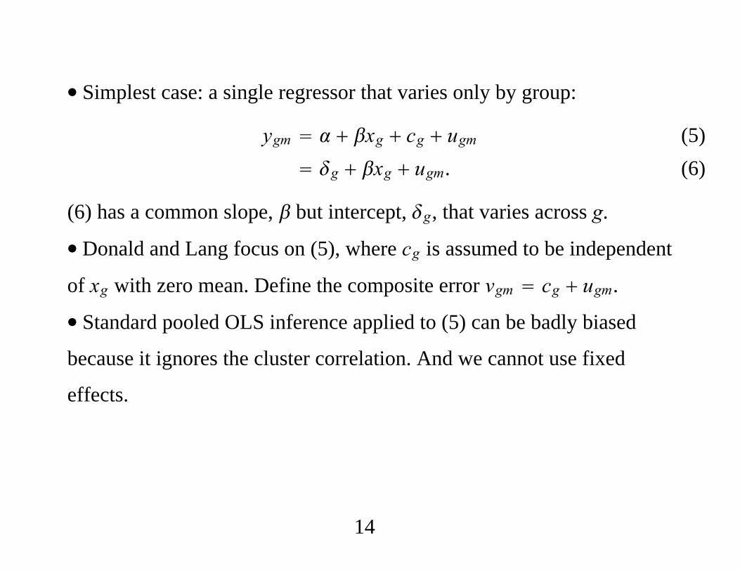
∙ Simplest case: a single regressor that varies only by group:
ygm xg cg ugm g xg ugm.
(5) (6)
(6) has a common slope, but intercept, g, that varies across g.
∙ Donald and Lang focus on (5), where cg is assumed to be independent
of xg with zero mean. Define the composite error vgm cg ugm.
∙ Standard pooled OLS inference applied to (5) can be badly biased
because it ignores the cluster correlation. And we cannot use fixed
effects.
14

∙ DL propose studying the regression in averages:
yg xg vg,g 1, . . . ,G. (7)
If we add some strong assumptions, we can perform inference on (7)
using standard methods. In particular, assume thatMg M for all g,
cg|xg Normal0,c2 and ugm|xg,cg Normal0,u2. Then vg is
independent of xg and vg Normal0,c2 u2/M. Because we assume
independence across g, (7) satisfies the classical linear model
assumptions.
15

∙ So, we can just use the “between” regression,
yg on 1, xg, g 1, . . . ,G. (8)
With same group sizes, identical to pooled OLS across g and m.
∙ Conditional on the xg, inherits its distribution from
vg : g 1, . . . ,G, the within-group averages of the composite errors.
∙We can use inference based on the tG−2 distribution to test hypotheses
about , provided G 2.
∙ If G is small, the requirements for a significant t statistic using the
tG−2 distribution are much more stringent then if we use the
tM1M2...MG−2 distribution (traditional approach).
16
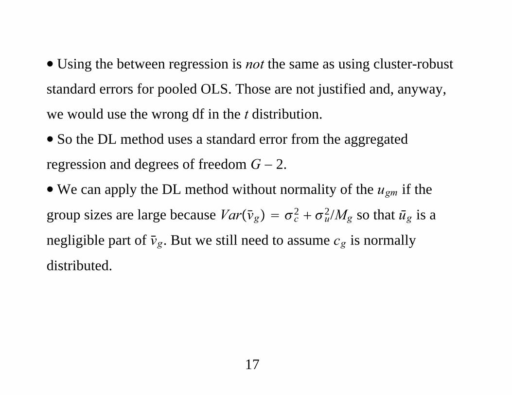
∙ Using the between regression is not the same as using cluster-robust
standard errors for pooled OLS. Those are not justified and, anyway,
we would use the wrong df in the t distribution.
∙ So the DL method uses a standard error from the aggregated
regression and degrees of freedom G − 2.
∙We can apply the DL method without normality of the ugm if the
group sizes are large because Varvg c2 u2/Mg so that ūg is a
negligible part of vg. But we still need to assume cg is normally
distributed.
17
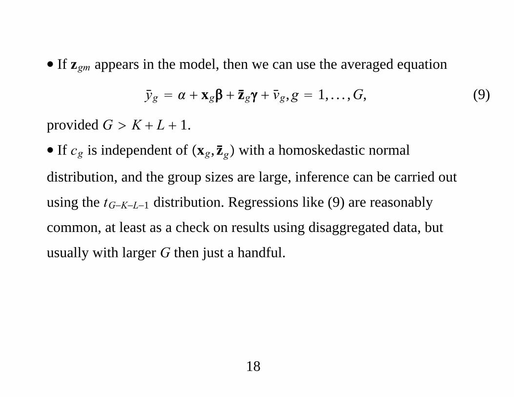
∙ If zgm appears in the model, then we can use the averaged equation
yg xg zg vg,g 1, . . . ,G, (9)
provided G K L 1.
∙ If cg is independent of xg, zg with a homoskedastic normal
distribution, and the group sizes are large, inference can be carried out
using the tG−K−L−1 distribution. Regressions like (9) are reasonably
common, at least as a check on results using disaggregated data, but
usually with larger G then just a handful.
18
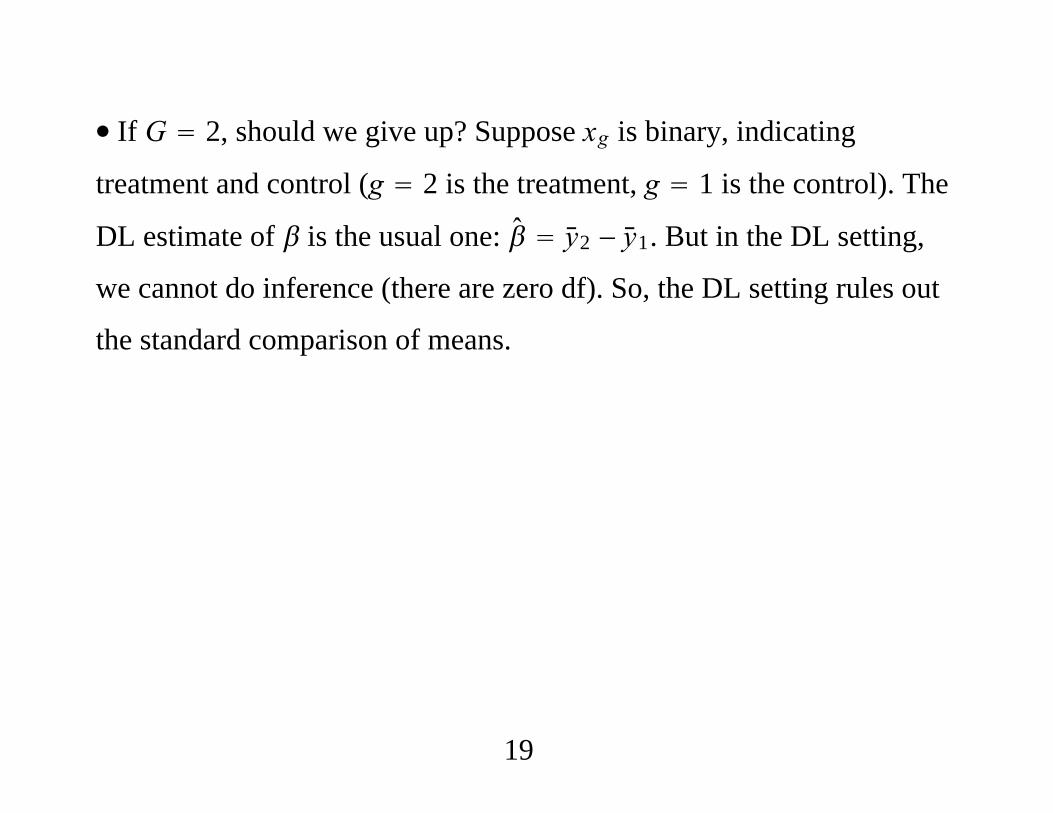
∙ If G 2, should we give up? Suppose xg is binary, indicating
treatment and control (g 2 is the treatment, g 1 is the control). The
DL estimate of is the usual one: y2 − y1. But in the DL setting,
we cannot do inference (there are zero df). So, the DL setting rules out
the standard comparison of means.
19

∙ Can we still obtain inference on estimated policy effects using
randomized or quasi-randomized interventions when the policy effects
are just identified? Not according the DL approach.
∙ If ygm Δwgm – the change of some variable over time – and xg is
binary, then application of the DL approach to
Δwgm xg cg ugm,
leads to a difference-in-differences estimate: Δw2 − Δw1. But
inference is not available no matter the sizes ofM1 and M2.
20
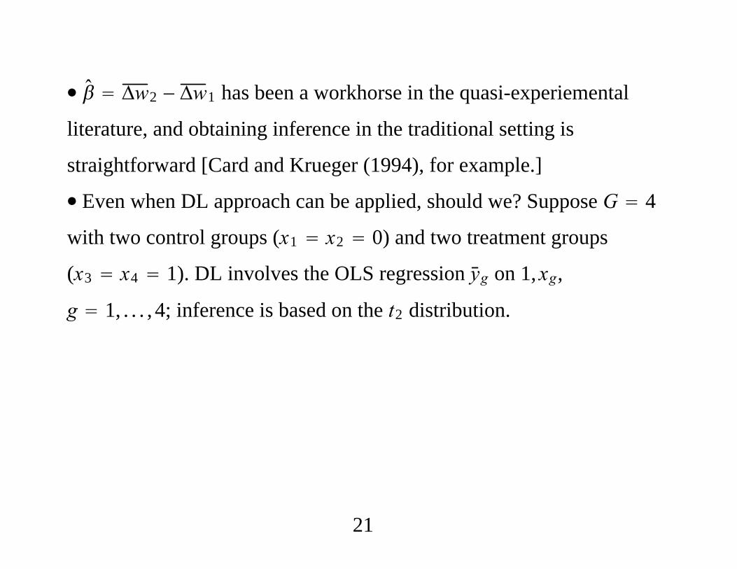
∙ Δw2 − Δw1 has been a workhorse in the quasi-experiemental
literature, and obtaining inference in the traditional setting is
straightforward [Card and Krueger (1994), for example.]
∙ Even when DL approach can be applied, should we? Suppose G 4
with two control groups (x1 x2 0) and two treatment groups
(x3 x4 1). DL involves the OLS regression yg on 1,xg,
g 1, . . . , 4; inference is based on the t2 distribution.
21

∙ Can show the DL estimate is
y3 y4/2 − y1 y2/2. (10)
∙With random sampling from each group, is approximately normal
even with moderate group sizes Mg. In effect, the DL approach rejects
usual inference based on means from large samples because it may not
be the case that 1 2 and 3 4.
22
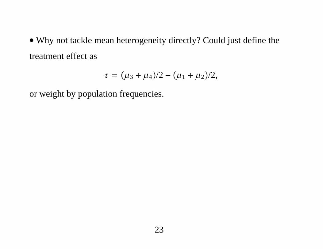
∙Why not tackle mean heterogeneity directly? Could just define the
treatment effect as
3 4/2 − 1 2/2,
or weight by population frequencies.
23
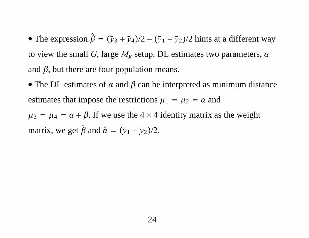
∙ The expression y3 y4/2 − y1 y2/2 hints at a different way
to view the small G, large Mg setup. DL estimates two parameters,
and , but there are four population means.
∙ The DL estimates of and can be interpreted as minimum distance
estimates that impose the restrictions 1 2 and
3 4 . If we use the 4 4 identity matrix as the weight
matrix, we get and y1 y2/2.
24

∙With large group sizes, and whether or not G is especially large, we
can put the problem into an MD framework, as done by Loeb and
Bound (1996), who had G 36 cohort-division groups and many
observations per group.
∙ For each group g, write
ygm g zgmg ugm. (11)
Assume random sampling within group and independence across
groups. OLS estimates within group are Mg -asymptotically normal.
25
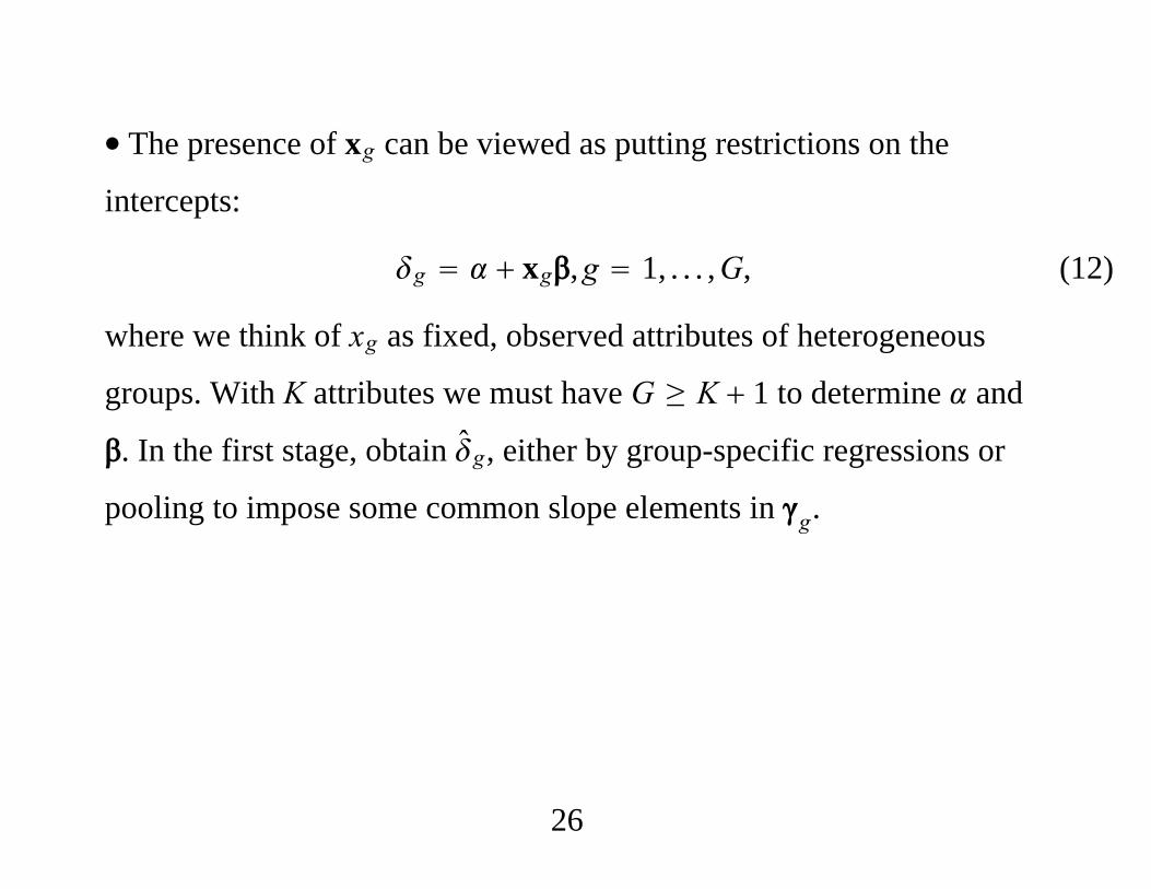
∙ The presence of xg can be viewed as putting restrictions on the
intercepts:
g xg,g 1, . . . ,G, (12)
where we think of xg as fixed, observed attributes of heterogeneous
groups. With K attributes we must have G ≥ K 1 to determine and
. In the first stage, obtain g, either by group-specific regressions or
pooling to impose some common slope elements in g.
26

∙ Let V be the G G estimated (asymptotic) variance of . Let X be the
G K 1 matrix with rows 1,xg. The MD estimator is
X′V−1X−1X′V−1 (13)
∙ Asymptotics are as theMg get large, and has an asymptotic normal
distribution; its estimated asymptotic variance is X′V−1X−1.
∙When separate group regressions are used, the g are independent and
V is diagonal.
∙ Estimator looks like “GLS,” but inference is with G (number of rows
in X) fixed with Mg growing.
27

∙ Can test the overidentification restrictions. If reject, can go back to
the DL approach, applied to the g. With large group sizes, can analyze
g xg cg,g 1, . . . ,G (14)
as a classical linear model because g g OpMg−1/2, provided cg is
homoskedastic, normally distributed, and independent of xg.
∙ Alternatively, can define the parameters of interest in terms of the g,
as in the treatment effects case.
28

4. Multiple Groups and Time Periods
∙With many time periods and groups, setup in BDM (2004) and
Hansen (2007a) is useful. At the individual level,
yigt t g xgt zigtgt vgt uigt,
i 1, . . . ,Mgt,
(15)
where i indexes individual, g indexes group, and t indexes time. Full set
of time effects, t, full set of group effects, g, group/time period
covariates (policy variabels), xgt, individual-specific covariates, zigt,
unobserved group/time effects, vgt, and individual-specific errors, uigt.
Interested in .
29

∙ As in cluster sample cases, can write
yigt gt zigtgt uigt, i 1, . . . ,Mgt; (16 )
a model at the individual level where intercepts and slopes are allowed
to differ across all g, t pairs. Then, think of gt as
gt t g xgt vgt. (17)
Think of (17) as a model at the group/time period level.
30

∙ As discussed by BDM, a common way to estimate and perform
inference in the individual-level equation
yigt t g xgt zigt vgt uigt
is to ignore vgt, so the individual-level observations are treated as
independent. When vgt is present, the resulting inference can be very
misleading.
∙ BDM and Hansen (2007b) allow serial correlation in
vgt : t 1, 2, . . . ,T but assume independence across g.
∙We cannot replace t g a full set of group/time interactions
because that would eliminate xgt.
31

∙ If we view in gt t g xgt vgt as ultimately of interest –
which is usually the case because xgt contains the aggregate policy
variables – there are simple ways to proceed. We observe xgt, t is
handled with year dummies,and g just represents group dummies. The
problem, then, is that we do not observe gt.
∙ But we can use OLS on the individual-level data to estimate the gt in
yigt gt zigtgt uigt, i 1, . . . ,Mgt
assuming Ezigt′ uigt 0 and the group/time period sample sizes, Mgt,
are reasonably large.
32

∙ Sometimes one wishes to impose some homogeneity in the slopes –
say, gt g or even gt – in which case pooling across groups
and/or time can be used to impose the restrictions.
∙ However we obtain the gt , proceed as if Mgt are large enough to
ignore the estimation error in the gt; instead, the uncertainty comes
through vgt in gt t g xgt vgt.
∙ The minimum distance (MD) approach effectively drops vgt and
views gt t g xgt as a set of deterministic restrictions to be
imposed on gt. Inference using the efficient MD estimator uses only
sampling variation in the gt.
33
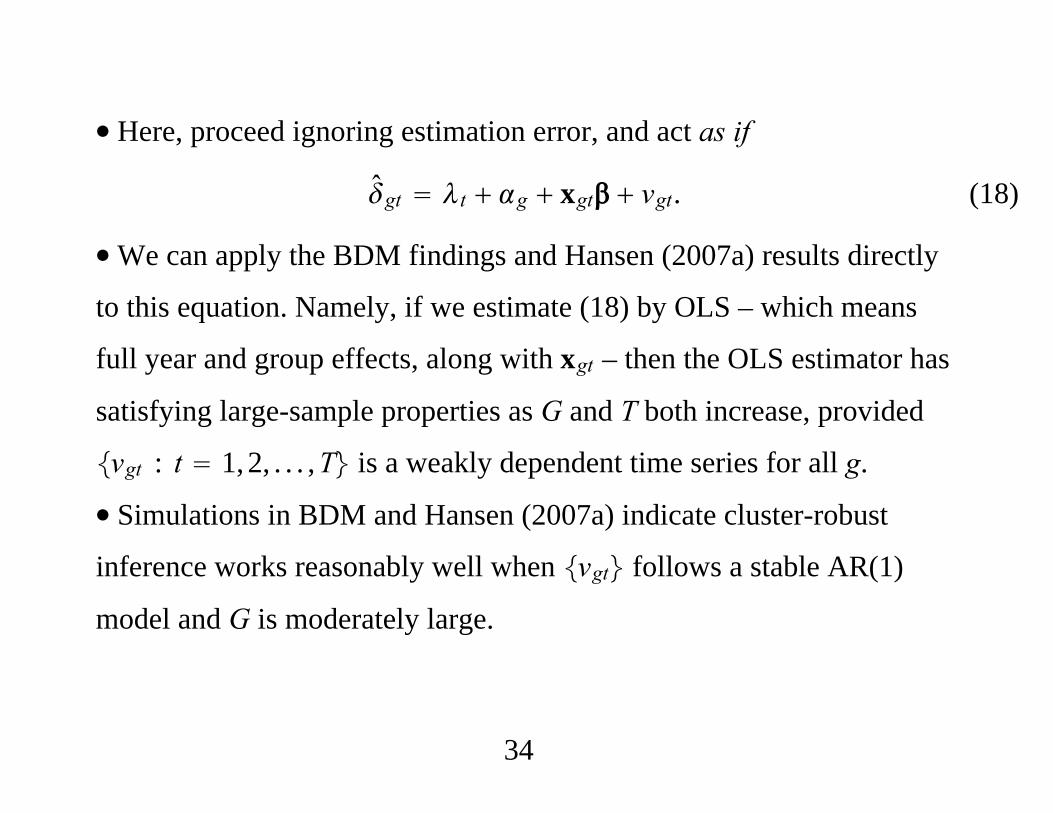
∙ Here, proceed ignoring estimation error, and act as if
gt t g xgt vgt. (18)
∙We can apply the BDM findings and Hansen (2007a) results directly
to this equation. Namely, if we estimate (18) by OLS – which means
full year and group effects, along with xgt – then the OLS estimator has
satisfying large-sample properties as G and T both increase, provided
vgt : t 1, 2, . . . ,T is a weakly dependent time series for all g.
∙ Simulations in BDM and Hansen (2007a) indicate cluster-robust
inference works reasonably well when vgt follows a stable AR(1)
model and G is moderately large.
34

∙ Hansen (2007b) shows how to improve efficiency by using feasible
GLS – by modeling vgt as, say, an AR(1) process.
∙ Naive estimators of are seriously biased due to panel structure with
group fixed effects. Can remove much of the bias and improve FGLS.
∙ Important practical point: FGLS estimators that exploit serial
correlation require strict exogeneity of the covariates, even with large
T. Policy assignment might depend on past shocks.
35
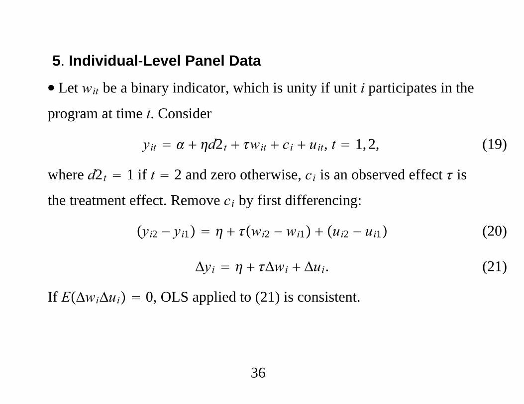
5. Individual-Level Panel Data
∙ Let wit be a binary indicator, which is unity if unit i participates in the
program at time t. Consider
yit d2t wit ci uit, t 1, 2, (19)
where d2t 1 if t 2 and zero otherwise, ci is an observed effect is
the treatment effect. Remove ci by first differencing:
yi2 − yi1 wi2 − wi1 ui2 − ui1 (20)
Δyi Δwi Δui. (21)
If EΔwiΔui 0, OLS applied to (21) is consistent.
36
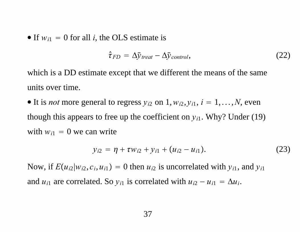
∙ If wi1 0 for all i, the OLS estimate is
FD Δytreat − Δycontrol, (22)
which is a DD estimate except that we different the means of the same
units over time.
∙ It is not more general to regress yi2 on 1,wi2,yi1, i 1, . . . ,N, even
though this appears to free up the coefficient on yi1. Why? Under (19)
with wi1 0 we can write
yi2 wi2 yi1 ui2 − ui1. (23)
Now, if Eui2|wi2,ci,ui1 0 then ui2 is uncorrelated with yi1, and yi1and ui1 are correlated. So yi1 is correlated with ui2 − ui1 Δui.
37

∙ In fact, if we add the standard no serial correlation assumption,
Eui1ui2|wi2,ci 0, and write the linear projection
wi2 0 1yi1 ri2, then can show that
plimLDV 1u12 /r2
2
where
1 Covci,wi2/c2 u12 .
∙ For example, if wi2 indicates a job training program and less
productive workers are more likely to participate (1 0), then the
regression yi2 (or Δyi2) on 1, wi2, yi1 underestimates the effect.
38
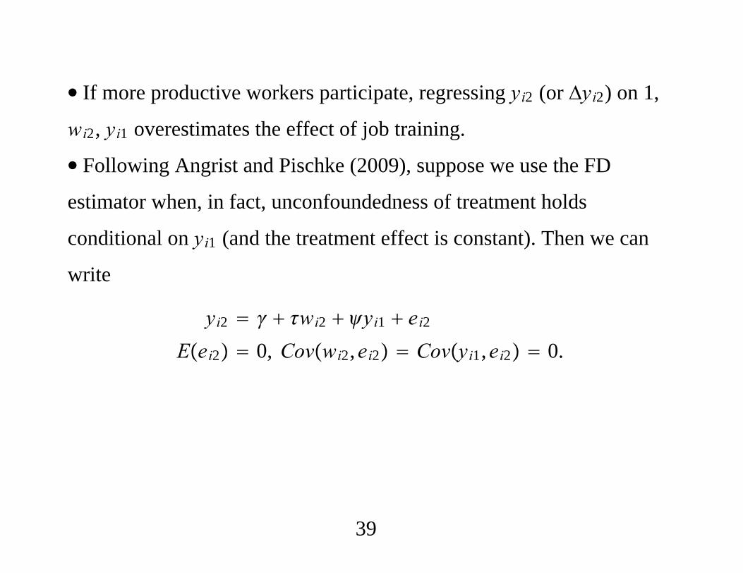
∙ If more productive workers participate, regressing yi2 (or Δyi2) on 1,
wi2, yi1 overestimates the effect of job training.
∙ Following Angrist and Pischke (2009), suppose we use the FD
estimator when, in fact, unconfoundedness of treatment holds
conditional on yi1 (and the treatment effect is constant). Then we can
write
yi2 wi2 yi1 ei2Eei2 0, Covwi2,ei2 Covyi1,ei2 0.
39

∙Write the equation as
Δyi2 wi2 − 1yi1 ei2≡ wi2 yi1 ei2
Then, of course, the FD estimator generally suffers from omitted
variable bias if ≠ 1. We have
plimFD Covwi2,yi1Varwi2
∙ If 0 ( 1) and Covwi2,yi1 0 – workers observed with low
first-period earnings are more likely to participate – the plimFD ,
and so FD overestimates the effect.
40

∙We might expect to be close to unity for processes such as
earnings, which tend to be persistent. ( measures persistence without
conditioning on unobserved heterogeneity.)
∙ As an algebraic fact, if 0 (as it usually will be even if 1) and
wi2 and yi1 are negatively correlated in the sample, FD LDV. But this
does not tell us which estimator is consistent.
∙ If either is close to zero or wi2 and yi1 are weakly correlated, adding
yi1 can have a small effect on the estimate of .
41
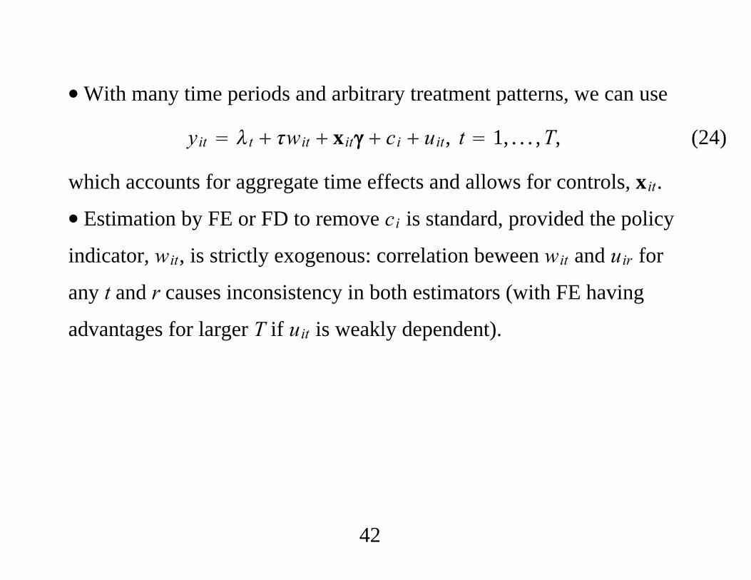
∙With many time periods and arbitrary treatment patterns, we can use
yit t wit xit ci uit, t 1, . . . ,T, (24)
which accounts for aggregate time effects and allows for controls, xit.
∙ Estimation by FE or FD to remove ci is standard, provided the policy
indicator, wit, is strictly exogenous: correlation beween wit and uir for
any t and r causes inconsistency in both estimators (with FE having
advantages for larger T if uit is weakly dependent).
42
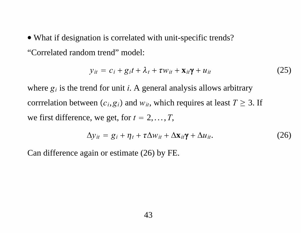
∙What if designation is correlated with unit-specific trends?
“Correlated random trend” model:
yit ci git t wit xit uit (25)
where gi is the trend for unit i. A general analysis allows arbitrary
corrrelation between ci,gi and wit, which requires at least T ≥ 3. If
we first difference, we get, for t 2, . . . ,T,
Δyit gi t Δwit Δxit Δuit. (26)
Can difference again or estimate (26) by FE.
43

∙ Can derive panel data approaches using the counterfactural
framework from the treatment effects literature.
For each i, t, let yit1 and yit0 denote the counterfactual outcomes,
and assume there are no covariates. Unconfoundedness, conditional on
unobserved heterogeneity, can be stated as
Eyit0|wi,ci Eyit0|ciEyit1|wi,ci Eyit1|ci,
(27) (28)
where wi wi1, . . . ,wiT is the time sequence of all treatments.
Suppose the gain from treatment only depends on t,
Eyit1|ci Eyit0|ci t. (29)
44

Then
Eyit|wi,ci Eyit0|ci twit (30)
where yi1 1 − wityit0 wityit1. If we assume
Eyit0|ci t0 ci0, (31)
then
Eyit|wi,ci t0 ci0 twit, (32)
an estimating equation that leads to FE or FD (often with t .
45

∙ If add strictly exogenous covariates and allow the gain from treatment
to depend on xit and an additive unobserved effect ai, get
Eyit|wi,xi,ci t0 twit xit0
wit xit − t ci0 ai wit,
(33)
a correlated random coefficient model because the coefficient on wit is
t ai. Can eliminate ai (and ci0. Or, with t , can “estimate” the
i ai and then use
N−1∑i1
N
i. (34)
46

∙With T ≥ 3, can also get to a random trend model, where git is added
to (25). Then, can difference followed by a second difference or fixed
effects estimation on the first differences. With t ,
Δyit t Δwit Δxit0 Δwit xit − t ai Δwit gi Δuit. (35)
∙Might ignore aiΔwit, using the results on the robustness of the FE
estimator in the presence of certain kinds of random coefficients, or,
again, estimate i ai for each i and form (34).
47

∙ As in the simple T 2 case, using unconfoundedness conditional on
unobserved heterogeneity and strictly exogenous covariates leads to
different strategies than assuming unconfoundedness conditional on
past responses and outcomes of other covariates.
∙ In the latter case, we might estimate propensity scores, for each t, as
Pwit 1|yi,t−1, . . . ,yi1,wi,t−1, . . . ,wi1,xit.
48

6. Semiparametric and Nonparametric Approaches
∙ Consider the setup of Heckman, Ichimura, Smith, and Todd (1997)
and Abadie (2005), with two time periods. No units treated in first time
period. Without an i subscript, Ytw is the counterfactual outcome for
treatment level w, w 0, 1, at time t. Parameter: the average treatment
effect on the treated,
att EY11 − Y10|W 1. (36)
W 1 means treatment in the second time period.
49
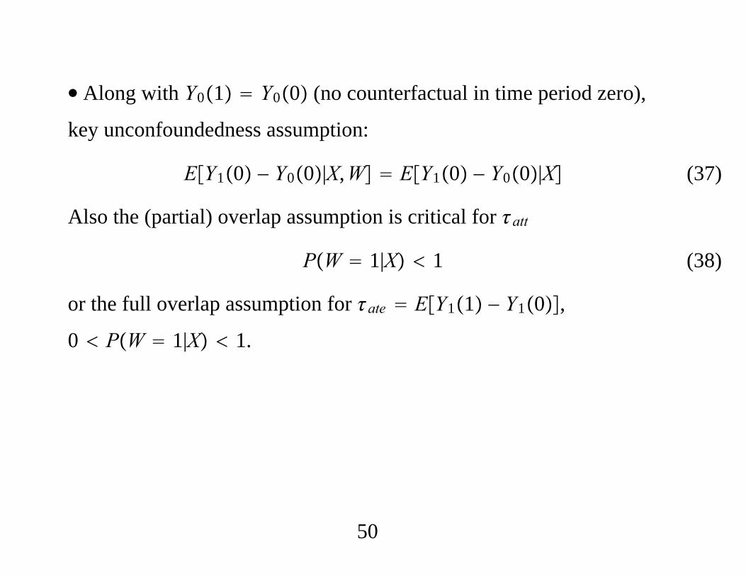
∙ Along with Y01 Y00 (no counterfactual in time period zero),
key unconfoundedness assumption:
EY10 − Y00|X,W EY10 − Y00|X (37)
Also the (partial) overlap assumption is critical for att
PW 1|X 1 (38)
or the full overlap assumption for ate EY11 − Y10,
0 PW 1|X 1.
50

Under (37) and (38),
att EW − pXY1 − Y0
1 − pX (39)
where Yt, t 0, 1 are the observed outcomes (for the same unit),
PW 1 is the unconditional probability of treatment, and
pX PW 1|X is the propensity score.
51
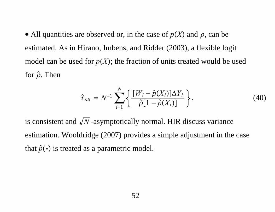
∙ All quantities are observed or, in the case of pX and , can be
estimated. As in Hirano, Imbens, and Ridder (2003), a flexible logit
model can be used for pX; the fraction of units treated would be used
for . Then
att N−1∑i1
NWi − pXiΔYi1 − pXi
. (40)
is consistent and N -asymptotically normal. HIR discuss variance
estimation. Wooldridge (2007) provides a simple adjustment in the case
that p is treated as a parametric model.
52

∙ If we add
EY11 − Y01|X,W EY11 − Y01|X, (41)
a similar approach works for ate.
ate N−1∑i1
NWi − pXiΔYipXi1 − pXi
(42)
53

7. Synthetic Control Methods for Comparative Case Studies
∙ Abadie, Diamond, and Hainmueller (2007) argue that in policy
analysis at the aggregate level, there is little or no estimation
uncertainty: the goal is to determine the effect of a policy on an entire
population, and the aggregate is measured without error (or very little
error). Application: California’s tobacco control program on state-wide
smoking rates.
∙ ADH focus on the uncertainty with choosing a suitable control for
California among other states (that did not implement comparable
policies over the same period).
54

∙ ADH suggest using many potential control groups (38 states or so) to
create a single synthetic control group.
∙ Two time periods: one before the policy and one after. Let yit be the
outcome for unit i in time t, with i 1 the treated unit. Suppose there
are J possible control units, and index these as 2, . . . ,J 1. Let xi be
observed covariates for unit i that are not (or would not be) affected by
the policy; xi may contain period t 2 covariates provided they are not
affected by the policy.
55

∙ Generally, we can estimate the effect of the policy as
y12 −∑j2
J1
wjyj2, (43)
where wj are nonnegative weights that add up to one. How to choose
the weights to best estimate the intervention effect?
56

∙ ADH propose choosing the weights so as to minimize the distance
between y11,x1 and∑j2J1wj yj1,xj, say. That is, functions of the
pre-treatment outcomes and the predictors of post-treatment outcomes.
∙ ADH propose permutation methods for inference, which require
estimating a placebo treatment effect for each region, using the same
synthetic control method as for the region that underwent the
intervention.
57