CLEARINGHOUSE FOR FEDERAL SCIENTIFIC AND TECHNICAL INFORMATION CFSTI DOCUMENT MANAGEMENT BRANCH 410.11

LIMITATIONS IN REPRODUCTION QUALITY

ACCESSION # RD C^¥ J76

n t WE REGRET THAT LEGIBILITY OF THIS DOCUMENT IS IN PART ^ UNSATISFACTORY. REPRODUCTION HAS BEEN MADE FROM BEST

AVAILABLE CGPY.

0 2. A PORTION OF THE ORIGINAL DOCUMENT CONTAINS FINE DETAIL WHICH MAY MAKE READING OF PHOTOCOPY DIFFICULT.

□ S. THE ORIGINAL DOCUMENT CONTAINS COLOR, BUT DISTRIBUTION COPIES ARE AVAILABLE IN BLACK-AND-WHITE REPRODUCTION ONLY.

n 4. THE INITIAL DISTRIBUTION COPIES CONTAIN COLOR WHICH WILL BE SHOWN IN BLACK-AND-WHITE WHEN IT IS VECESSARY TO REPRINT.

S. LIMITED SUPPLY ON HAND: WHEN EXHAUSTED, DOCUMENT WILL BE AVAILABLE IN MICROFICHE ONLY.

I. LIMITED SUPPLY ON UlANO: WHEN EXHAUSTED DOCUMENT WILL NOT BE AVAILABLE.

□ 7. DOCUMENT IS AVAILABLE IN MICROFICHE ONLY.

□ 8. DOCUMENT AVAILABLE ON LOAN FROM CFSTI ( TT DOCUMENTS ONLY).

□ s. NU S/M PROCESSOR: CM&J

CO a DO

to

I z'

REVISIONS AND EXTENSIONS TO THE SIMPLEX METHOD

(With Side-lights on Proyranaing Techniques)

Nn. Orchard-Hays

P-562 V y

2 Septeaber 1954 I

\

Approved for OXS

nsyy /nop ^L

HARD COPY MICROFICHE

DDC

QQC-lfiA 0

-7^ ßiJflD ßvtßwuiU** WOO MAIN ST. • SANTA MONICA • CAUVOINIA

)

• •

■

■

P-562 9-2-54

SDMARY - 1 -

The tiaplex tlgoritha for solving lineir progranning

probleat aay bt aodifled la varioat «ays to provide algorithas

for various aaxiliary purposes. la partiealar, the use of the

dial systea allows arbitrary changes to be aade in the right

hand aoabors of the restraiat equations. Aa allied algoritha —

called paraaetric linear prograaaing — allows desired changes

to be introduced gradually in such a way as to aaintain feasi-

bility aad optiaality at all tiaes. Siailarly, changes in the

optiaiiing fora can be aade either arbitrarily or in such a way

as to aaintain optiaality. If the siaplex aethod is viewed as

being coaposed of certain rather coaprehensive operations, then

all these variations can be stated in teras of the following set

of those abstract or pseudo-operations, where the order of oxe-

cation aay vary for difforoat purposes.

(1> Developaoat of a pricing vector or vectors.

(2) Choice of aa Index s of soae coluan vector P. not v S

in the present basis.

(3) Representation of the vector P in teras of the s

present basis.

(4) Choice of aa iadex r of soae coluan P. in the Jr

present basis.

(5) Change of basis, with P replacing P. , or change Jr

of the right head aeabers of the restraint

equations.

It is suggested that a breakdown of this type has iaportant

iaplications for flexibility and adaptability in a coaputer code.

REVISIONS AND EXTENSIONS TO THE SIMPLEX METHOD

(With Side-lights on Progranning Techniques)

*

Since this session enphisizes coaputing techniques, I

will tike • little tine to explain a problen which I believe

should be wore widely understood by people who require large-

scale computations« As this concerns the economics of machine

utilization, it is perhaps not entirely inappropriate.

When the original formulator of a large problem — usually,

and hereafter, called the 'customer* — brings his monstrous

brain child to be prepared for machine calculation, he is full

of assurances that this example is the forerunner of several

entirely similar ones for which the same program can be used.

The customer is entirely honest in this but unfortunately what

usually happens is the following. Just as the routine is nearly

finished, the customer rushes down with some 'trivial* last-minute

changes. These having been more or less graciously accommodated

and the code finally checked out on the machine, it turns out

that certain numerical difficulties crop up. Change is piled

on change and eventually an acceptable set of answers is obtained

but the code has lost all elegance or clarity which it may ever

have possessed. In the meantime, of course, the customer has

been pondering deeply over the imperfections in his method v-hich

these difficulties have revealed and, when he presents the next

example, he has changed a few formulas, refined a few rules,

but these he suggests are mere details which the coder can

incorporate in the program before running the next case. At

this point, the programmer must consider whether it is not

cheaper to start all over.

P-562 9-2-54

Page »2

No« having played both the role of prograaaer and, in part,

of cuftoaer, I have repeatedly been faced with the problen of

aaking extensive changes in a large code. One atteapt at

■aking these less painful and less expensive has coae about

as a result of considerable experience in coding up routines *

for linear prograaaing probleas to be solved with the simplex

aethod oa the IBM 701 Qe,fJ. Since such a code aay involve -

upwards of 5000 individual coaaands in its entirety, the prob-

lea is by no aeans a simple one.

One iaportaat phase of the prograaaing art is the use of

what are called asseably routines. Since, for aany reasons,

it is virtually iapossible, in practice, to write down the

required list of coaaands in aachine code, soae sort of con-

venient language interaediate between ordinary written in-

strnctions and aachine coaaands is devised. Then a program

is prepared — at considerable initial cost — which can

'read* the interaediate language and translate it into

aachine code. Subsequent probleas are then coded in the

interaediate language and, as a preliminary step in the com-

putations, the code is processed by the asseably routine.

Everytiae it is necessary to re-asseable the code, the cost

of the code is increased by aachine tiae as well as programmers'

time.

In all prograas which are to be assembled, the notion of

regions is proainent. A region is a group of consecutive aeaory

P-S62 9-2-54 Page »3

cells set aside for soae more or less well-defined set of

quantities — connands or numbers or sometinei both. Regions

are usually simply created at mill as need arises« the reason

that they are needed at all being that the logical layout of

a complex procedure can be conceptualized only in terms of

functional parts that make up the whole. Once a region has

been coded up and checked out (with of course appropriate

devices for implementing its use), it takes on a new character

— it becomes in fact an abstract, or pseudo-operation which

is henceforth available for use in future problems. By a

pseudo-operation is meant some arithmetic, logical, or utility

activity which requires more than one actual machine order.

For semantic purposes, let us denote adjustments in a

program necessitated by coding errors as corrections, and those

necessitated by procedural changes as modifications. Then once

a particular region — i.e. a pseudo-operation — has been

checked out, there are no more corrections to be made provided,

of course, that the assumptions on which it is based are always

observed. Now procedural changes do not usually involve any

modification in lower order pseudo-operations such, for example,

as adding two vectors together. The modifications occur — or

should do so if proper planning is done — in what are called

control regions, the higher order abstractions which control

the order and frequency of use of the subservient regions. The

big difficulty is that there is often not a sufficiently compre-

hensive picture of the whole problem shared by the customer and

P-562 9-2-54

Page *4

coder at the outset to allow proper planning, that is, the

control regions do not bear the proper relationship to the prob-

leas at hand.

At this point I aust mention that it is possible to use a

pseudo-code which is never assembled into machine language at

all but which requires the use of an interpretive routine for

the actual running of a problem — a method widely practiced.

This interpretive routine usually recognises some fairly com-

prehensive list of commands but requires that a great deal be

explicitly specified and is very time-consuming in operation

for large, special-purpose codes. Moreover, extensive changes

axe nearly as difficult in a universal pseudo-code as in machine

code. What is needed is a pseudo-code which takes advantage

of the extensive background of conventions which inevitably

arises in protracted computations and calculations along fixed

lines. However, it should be possible to couple together var-

ious parts of the code on demand. Just as an interpretive

routine does. In short, the code should be analogous to the

mathematician's thought processes. In this way variations in

the structure of the main procedure are easily arranged with a

minimum of coding and check-out time, and time is not wasted in

repeatedly interpreting the same thing while running the Job.

We now have a 701 code based on this philosophy. The pseudo-

operations mentioned below reflect its major structure.

Time limitations force me to make the seemingly reason-

able assumption that those interested in this paper are already

familiar with the simplex method. However, since we use a

P-562 9-2-54

Page *5

slightly different elgorithn than nost others, let ne Just

briefly sketch the way in which we set up the coaputttions

Qa.c.e.fl. There is, first of all, a linear form to be

optimized, and I will convene that, as written, it is to be

ninimized.

(6) J =

a0|xj - min*

This is to be done subject to two classes of restraints on the

n variables xj.

(7) Xj ^ 0 , J = 1, .. .t fti

(6) n y ajiX« = bi , i = 1, •••, m, J=l J J

where the ajj and bj (i = 0, 1, ..., m; J s 1, ..., n) are

specified and we further assume, without loss of generality,

that all the b* > 0.

Let us assemble all the a^j from (6) and (0) into one

(m-M)X(n-fl) matrix P whose first column we make a unit vector.

(9) P=

1

0

ol

'11

'ml

• • •

• • •

on

In

'mn

" [/o* Pl* ,*,, PBJ*

The columns we have called Pj (J =0, 1, .... n) where P0 is

the unit vector. With P0 we will associate a new variable x0

and form the column of variables

(10) X = J x0, X] xn ̂ •

•Braces will be used to denote column vectors and parentheses to denote rows.

P-562 9-2-54 Ptge »6

The right hand side will be denoted by the colunn vector

(11) Q =j 0, bj b, -.

Now the problem way be stated as:

Maximize x0 subject to (7) and the matrix equation

(12) PX ■ Q.

I will ignore the questions of determining the rank of P

and obtaining some feasible solution to (12), i.e. oae which

satisfies (7). All this is taken care of by phase one of the

simplex method, when necessary ria,c:2j. Let us merely assume

that P has rank »»-1 and that a basic feasible solution is at

hand which consists of a non-singular basis matrix B and an

associated solution vector V * B-^Q where

<13) •"['V'JI PJ.] V'.' is formed from a subset of the columns Pi. Let the values of

the corresponding variables x. (i = 0, 1, ..., m) be V|, with

all other xj s 0. That is,

(v0 = x0)

by /3ik.

(14) V = |v0, vj, ..., vB

Further denote the elements of B~'

(15) B-l = {fiik)

and any particular row of B~* by^.,

(16) /tfj = (>*|0t ^jjt •••! *im)»

Note that the first column of B"1 is also a unit vector, that is,

The ÜXIi row ^o of the inver»0 *• called a pricing vector.

If we define

(17) S. s >» P = /^Ir«! J • J ^ ^ok'kj J ~1| * • ■ i n

I

P-562 9-2-54

Page »7

then the flnt ilaplex criterion it stated at follows:

J

If £. < 0 for snyj, then the value of x0 «ill

(10) be increased (or at least not decreased) if P

is introduced into B.

If all S. 2. 0, then x s TA is max. j o o

If some s < 0, the usual rule if to choose an index s by

(19) S = min £. < 0 taking saallest iadex in case S J J

of ties.

Then P, is introduced into B. !■ erder to choose an index r of

lone vector P. in B which P( is to replace, we express Pf in

leras of B.

0) B-1Pf = Y = jy0, yl yl .

e second siiplex criterion (in its-'sinplifled for») is

(20)

Th

now expressed as:

If «ny y^ 0 for i j* 0.

let Oi = ^i/yi for those y|> 0 and i> 0

= -♦• oo otherwise.

(21) Then Q - min 0. taking snallest index in case r i *

of ties.

If all y,^ 0, then the value of xA has no i o

upper bound.

Assuming that x0 is bounded, then P. is eliwinated fron B and

replaced by Pg giving, after the change of basis, the new

solution

(22) B(V - ©ry) * •rP$ = BV = Q,

with a new value of x ,

(23) vo= vo * «r^. i v0.

P-562 9-2-54

Page »8

Those fenlliir with the sinplex theory will note that,

in using the siaplified second criterion, I have ignored the

possibility of endless cycling through a recurring series of

bases — a natter which has been discussed at considerable

length in various papers ["la, 2, 3, 4l . We feel, however,

that this is a very iaprobable eventuality there being, to date,

only two extrenely synthetic exanples (by Alan Hoffman and

Philip Volfe) in which cycling has occurred. It is my view

that non-convergence of the sinplex iterative process is only

the Uniting case of slow convergence. Until we understand

nore clearly why sone problens converge quickly and others —

which appear to be of sinilar structure — take nore iterations,

there seens little point in conplicating a code to provide for

the unlikely case while ignoring the nore frequent difficulty of

slow convergence. While either Dantzig's or Charnes* method

[jit2l for rigorously resolving ties in choosing the index r

will prevent absolute degeneracy — and hence avoid cycling —

they still pernit an inpossible nunber of iterations, fron a

practical standpoint, in bad cases.

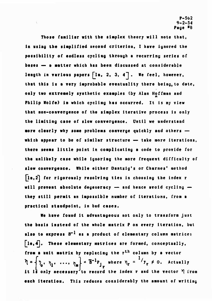
We have found it advantageous not only to transform Just

the basis instead of the whole natrix P on every iteration, but

also to express B"^ as a product of elenentary colunn natrices

rie(4l. These elenentary natrices are forned, conceptually,

fron a unit natrix by replacing the rth colunn by a vector

^ s J 7 , >| *lmf*~l?} "here ^r = 'if * 0. Actually

it is only necessary to record the index r and the vector *! iron

each iteration. This reduces considerably the amount of writing

P-562 9-2-54

Ptge »9

necessary to record B"^ and requires less rending for the

first several iterations. This form of the inverse is also

convenient for several other purposes, including calculating

the effects of various transformations on a systen and facili-

tating checking and restarting procedures — the latter being

extreaely important in practice. This product form has been

written up and circulated rather widely r5 ; so that I shall not

develop the details of it here. It seemed necessary to remark

on it however, since it requires the redevelopment of the

pricing vector /^0 on each iteration and certain statements to

follow night not be clear unless this fact were understood.

Similarly, when a P is chosen, it is still in its original

form and must actually be transformed into the vector Y by

applying B~ .

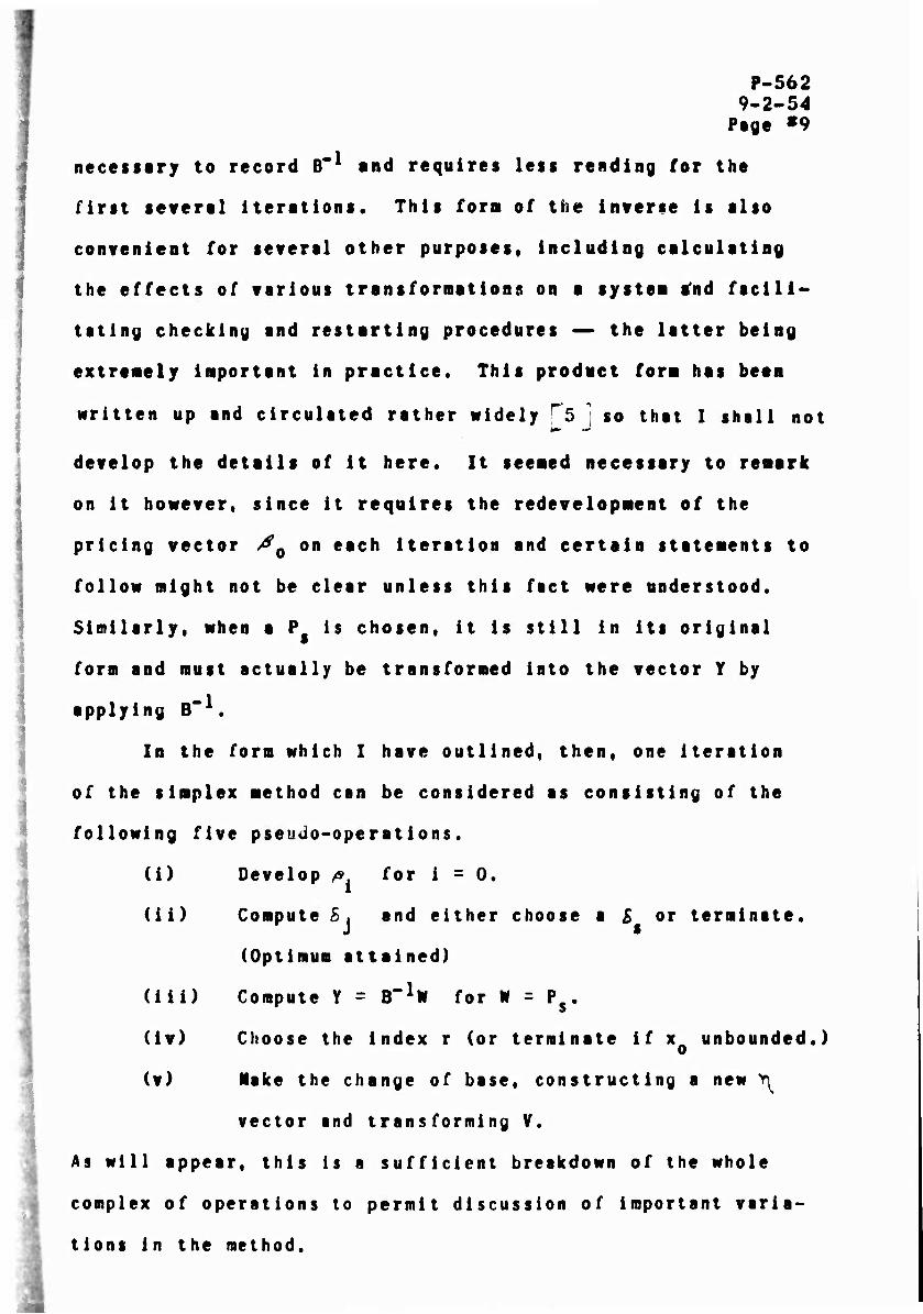
In the form which I have outlined, then, one iteration

of the simplex method can be considered as consisting of the

following five pseudo-operations.

(i)

(ii) Compute S. and either choose a £ or terminate

(Optimum attained)

Develop /» for i = 0.

(iii)

(iv)

(v)

Compute Y = B"1* for W = Ps.

Choose the index r (or terminate if xA unbounded.) o Make the change of base, constructing a new ^

vector and transforming V.

As will appear, this is a sufficient breakdown of the whole

complex of operations to permit discussion of important varia-

tions in the method.

P-562 9-2-54

Ptge '10

The solution m( a linear prograaning problea is often

merely the first step in the investigation of a larger economic

or administrative problea. As one example, a linear program

may contain a parameter which can be changed to give different

linear approximations to some non-linear relationship among the

variables. If the non-linear function is continuous, then it

is expected that optimal programs »ill differ only slightly for

small changes in the parameter. It is clearly desirable to be

able to introduce slight variations using a previous optimal

solution as a starting point, rather than to consider each

parametric chaage as a whole new programming problem.

There are three essentially distinct questions of this

kind each of which can be approached in two ways. Of the result-

ing six problems, the following four are the most amenable to

automatic computing schemes. We refer to these as post-opti-

mality problems and the techniques for handling them as para-

metric linear programming or PLP.

Given an optimal solution BV = Q to the problem of maxi-

mising x0 subject to (7) and (12), then:

Pr.l) How much can Q be changed in some specified way before

the basis B is non-feasible, i.e. before the necessary

change in V makes some v. ^ 0?

Pr.2) If an arbitrary change is made in Q and the basis becomes

non-feasible, how can this be corrected or it be deter-

mined that the whole new problem is non-feasible?

Pr.3) How much can the form (6) be changed in some specified

way before the solution is no longer optimal, i.e. before

P-562 9-2-54

Page »11

i

I

the necessary change in fi makes some %. < 0? o J

Pr.4) If some arbitrary change is made in the «Q.*«. how can this

be accounted for in B"1 (more particularly in 4 ) so that o

vectors not in the basis — or even in the original system

— can be priced out?

We could also ask a pair of similar questions about changes in

the original system (8), i.e. in the matrix P with the zero-th

row and the iero-th column excepted. However, for changes

outside the basis B, the problems are trivial whereas, for

changes within B, the general case is quite messy. It is

better to improvise tricks for the particular model at hand or

else start all over, in the latter case. Consequently, we will

make no further mention of parameters in the left members of

the restraint equcfions although they are used fairly frequently.

Pr. 2 can be answered very quickly. Simply make the

desired change in Q and re-solve for V. If the resulting V

contains no negative elements, all is well since, in any event,

the pricing vector /s remains unchanged. Hence we still have

all &j Z 0 and the solution remains optimal as well as feasible.

If some vj *■ 0, then apply the dual simplex algorithm to regain

feasibility, making the necessary changes of basis. If this

cannot be done, then no feasible solution exists for the new

right hand side.

The dual algorithm, as the name implies, operates on the

dual problem, but does so in terms of «he primal system so that

all computations can still be carried out in (ir*-l)-space instead

P-562 9-2-54

Page '12

of (n+l)-tpace which is typically much larger Qb.fJ. Without

attenpting to reconstruct the theory of the dual, let us note

the following pertinent facts concerning the complete dualized

system with notation consistent with the above.

PRIMAL DUAL n ■

Objective: naxinize x0 = - 2lZ 1oJxJ ■inl"lze z ~ Z bi^"<

Feasibility: Vj a 0 for i ^ 0 Sj 2 0 for J ?t 0

Optinality: 6, ^ 0 for J ^ 0

Criterion for inprovewent: S = win £. << 0

Criterion for 6 - win Tl/y (1/0) elinination: y^O

Vj i 0 for i >* 0

vr = win v < 0

oJ o 1 © - «In —* - Bin -*-*-

V0 rJ r J

Unbounded case: All y. < 0 is

All )rrJ>

The dual algorithn can now also be stated in terms of five pseudo-

operations which I number in a manner analagous to those for the

regular primal algorithm.

(iva) Choose the index r, or terminate. (Optimum attained)

(i) Compute /^j for 1 = 0 and r.

(iia) Choose 0 , or terminate if no ^.P.< 0. (Optimum • •' unbounded)

(iii) Compute Y = B-1* for W = Pf.

(v) Make the change of base, constructing a new 7) vector

and transforming V.

Pr.l is handled by a very similar algorithm but with

somewhat more finesse. Let q be the vector of changes which

it is desired to make in Q. Then assume that an optimum

solution BV = 0 has been obtained for the restraints

P-562 9-2-54

Page * 13

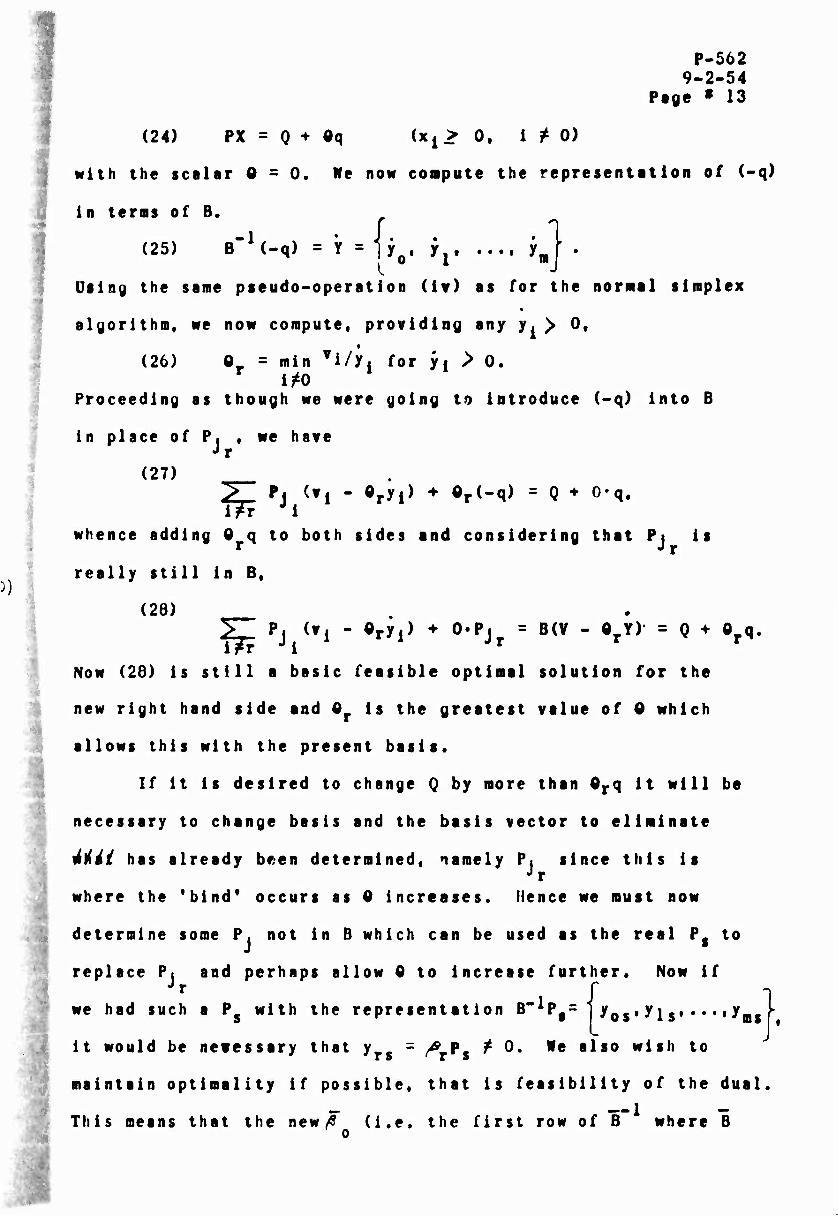
(24) PX = 0 + öq (xj > 0. i ^ 0)

with the scalar 0=0. We now compute the representation of (-q)

in terms of B.

(25) iT^-q) = if = jyo. ^ y^

Using the same pseudo-operation (iv) as for the normal simplex

algorithm, we now compute, providing any y. > 0,

(26) 0_ = min vi/yi for yj > 0. i^O

Proceeding as though we were going to introduce (-q) into B

in place of P. , we have Jr

(27)

whence adding 0 q to both sides and considering that Pi is r j j

really still in B,

(28) Zjl Pj <vi - «ryi> * 0-Pjr = B(V - OrY) = 0 ^ Orq.

Now (28) is still a basic feasible optimal solution for the

new right hand side and Qr is the greatest value of 0 which

allows this with the present basis.

If it is desired to change Q by more than Orq it will be

necessary to change basis and the basis vector to eliminate

4lt4i has already been determined, namely Pi since this is Jr

where the 'bind* occurs as 0 increases. Hence we must now

determine some P. not in B which can be used as the real Ps to

replace P, and perhaps allow Q to increase further. Now if Jr

we had such a Ps with the representation B" Pfs ' y0f•Xi

it would be netessary that y.. = A.P. t 0. Me also wish to

maintain optimality if possible, that is feasibility of the dual.

This means that the new ^ (i.e. the first row of B where B o

, .. • i OS ft

■

P-562 9-2-54

Page »14

it formed fron B by replacing P, with P ) must have the Jr s

property that>5"0Pj^ 0 for J = 1, .... n. The rules for

elimination give

y /*P

Jr Jr 7rs r s

Hence we should choose y < 0 since y = £ ^ 0. From this it rs os * is easy to show that the index s is chosen by the same rule (iia)

as was used in the straight dual algorithm above.' Hence the PLP

algorithm for changes in the right hand side goes as follows,

where a new pseudo-operation (vi) is needed,

(iii) Compute Y = B'1* for W = (-q).

(iv) Choose the index r, or terminate, (max Q unbounded

with present B.)

(vi) Subtract 0rY from V and add 0rq to Q.

(i) Computed, for i = 0 and r.

(iia) Choose 0 . or terminate. (max x0 unbounded with

present 0.)

(ili) Compute Y = B"1« for W = Ps.

(v) Make the change of base, constructing a new /|

vector and transforming V.

/ The following theorem is of considerable interest t^r \ ^ this type of PLP.

Theorem; If the choice of r in (26) is unique (assuming

same y^ > 0) and

(a) if ^-Pj < 0 for some J s 1» ..., n,

then there exists a finite range of 0. « *© ^6Tt£f

P-562 9-2-54

Page »15

for which the »olutlon obttlned by replacing

P. in B by Pf (chosen by (11a)) if both feasible r

and optimal; or

(b) if all a P > 0, then there is no feasible solution "r j -

lor 0 > 0 . r A constructive proof of this theorem is quite straightforward

and even provides a formula for the value of 6 , This proof can

be found in another paper which I prepared about a year ago

and will be omitted here fll.

In order to consider Prs. 3 and 4, let us denote the top

row of P — i.e. the coefficients of x and the ■inimizing form —

by

^o ~ (1» ■ol* Äo2, •••• •on^

If certain (or all) of the a0. are to be altered by proportionate

amounts cr, of a parameter 0, let J

«r= (O.^j,^ <rn)

and consider the matriA F as having \tt top row given by

Let a given basic feasible optimal solution to the

original problem be BY = Q which is then a solution for 0=0.

Now if 0 is increased, Bt and hence B , is changed. But due

to the special structure of B — i.e. with its first column

a unit vector — the only change in B will also be in its

top row/tf0( or as n economist would say, in the shadow prices«

This can be seen from the following schematic diagram of B'1

compared with B. The matrix A is simply B with its first row

and first column deleted.

P-562 9-2-54

Page »16

1 (•.•••••. OJi "J.

0

0

-1 (£ .... A )'

ol on

.-1

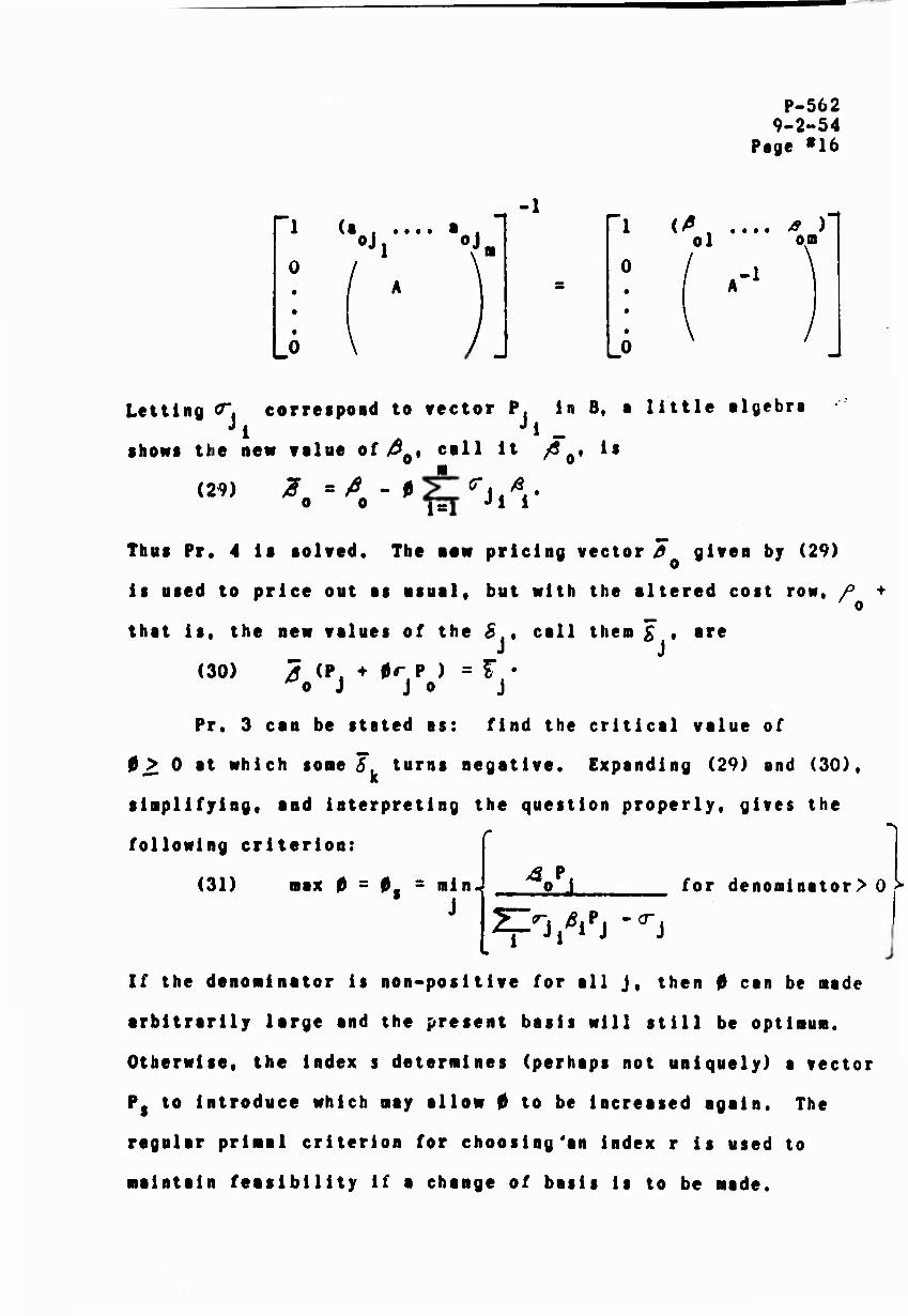
Letting cr correspond to vector P. in B, a little algebra Ji Jl -

shows the new value o(/$0, call it /S 0, is

(29) J = A - 0 1 = Ji i

Thus Pr, 4 is solved. The now pricing vector 0 given by (29) o

is used to price out as usual, but with the altered cost row, /> + o

that is, the new values of the £ , call them £ , are

(30) 7 (P. *• 0r P ) = F • ^o J Jo J

Pr. 3 can be stated as: find the critical value of

0^ 0 at which some J turns negative. Expanding (29) and (30),

siaplifying, and interpreting the question properly, gives the

following criterion:

(31) wax 0=0.= min J

Vi for denoninator> 0

Vipj "^ J i Ji

If the denominator is non-positive for all J, then 0 can be made

arbitrarily large and the present basis will still be optimum.

Otherwise, the index s determines (perhaps not uniquely) a vector

Ps to introduce which may allow 0 to be increased again. The

regular primal criterion for choosing'an index r is used to

maintain feasibility if a change of basis is to be made.

P-562 9-2-54

Pige »17

I might remark in passing that the use of the product

form of the inverse in machine computations is ideal for

computing the row vector^g in (29) or the sum vector > ^j ß^

for use in the denominator of (31).

The algorithm for Pr. 4 is the same as the one for the

regular simplex method once the specified amount 0 of cT* has «I

been added to each a . and the correction (29) made in the

inverse. For Pr. 3, we need only to substitute the computations

involved in (31) for the pseudo-operations (i) and (ii), i.e.

we replace the first simplex criterion with (31). This is only

to be expected, of course, for once an optimum solution has been

obtained to the original problem, the first simplex criterion

has nothing more to offer -— its function is completed.

In summary, let me again re-emphasize that organizing

computational sehr es in terms if fairly comprehensive pseudo-

operations, such as have been indicated, is advantageous for

the coder, the mathematician, and the economist. There is,

of course, nothing new in the notion either of regional coding

or of abstract or pseudo-code. My complaint is that the organi-

zation of codes into regions or blocks — and the devices used

to couple them together and execute them — is all too often

based on short-view expediency or established usage rather than

on the true nature of the problem? for which the program is

designed. Furthermore, I suspect that this is also true for

many problem formulations, apart from whether machine codes are

written or not. Mathematicians, economists, and others who are

potential customers for the services of a machine computing

group should be interested in being as much as possible in

P-562 9-2-54

Page »10

rapport with all those engaged in solving their problems. All

variations to date on the basic simplex algorithm, for instance,

can be expressed in terns of Just a few of our pseudo-operations,

very few more than we have already mentioned. Consequently, if

everyone's work is organixed and planned along these lines, then

modifications involve only a reshuffling of large blocks of

already proven code. Furthermore, this sort of breakdown enhances

the clarity of one's insight into the theory which underlies all

these linear programming techniques — namely that of a system

of linear inequalities in non-negative variables and its dual.

(Actually, in applying the simplex method, the systems are sets

of linear equalities.) For example, the parameters Q and 0 which

we have discussed are really variables which are involved implicitl

— but intimately — in any optimization problem with linear

restraints in non-negative variables. When working with feasible

solutions of the primal system, the variable 9 is made as large

as it is possible to do and still maintain feasibility; the

variable 0 plays the same role for feasible solutions of the dual.

In fact, as already noted, the change in the maximand x0 for the

former case is -0£ > 0, whereas the change in the minimand z

— which is really the same variable in the complete dualized

system -* is given by 0vr £ 0 in the latter case. Both Q and 0

are quotients with the pivot element, yrg, for denominator in

either the regular primal or straight dual algorithms. When

both systems are feasible, i.e. when the whole dualized system

is optimal, then any desirable change in basis can only give

another optimal solution, both 9 and 0 being zero and yr$ being

any non-iero number. If changes are made in the right-hand

P-562 9-2-54

Page «19

side 0 or the cost row y0 . then parametric programming provides

slightly different formulas for 0 or 0 to maintain optimality,

as discussed above.

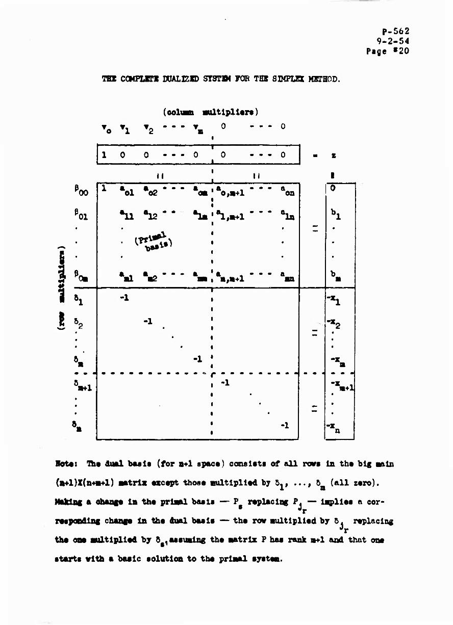
To conclude, the complete dualized system is displayed

in a form consistent with the preceding notation and arrange-

ment of the original problem. For simplicity, it has been

assumed that the basis B consists of the first m+1 columns

of P. It is hoped that a careful perusal of this tableau

will be as helpful to those readers who have not yet consider-

ed it as it has been to me in observing the remarkable

relationships that exist in the type of problems with which

we have been concerned. A full explanation of these relation-

ships which the tableau is intended to display can be found

in reference Nl .

.

p.562 9-2-54

Page »20

TBK COMPLET DÜALEXD STSTBf TOB THB SIMPLEX METHOD.

( COIUM aalt Ipl Urt)

To Tl T2 ••- ^ ^ o --. 0

1 0 0 - - - 0 0 - - - 0 ■ t

II I M 1

"oo 1 aol •o2--- •o.;fto^i--- ann 0

eoi •u •la-- •ta»*!^!'-- ha bl •

•

•

•

•

•

•

•

•

•

1l,fl" •i v- •ilV^i"" a«n b.

S »i -i -*i

1^ • • •

-i •

• •

- -»2 • • •

». -x • -X

8«1 •

mmfmmmmmm

1 'I

i

•

• |

-1

•

"a

Wot«; Th« dual bMlt (for n+l spao«) oooaltti of all roirs in tht big aale

(a+DXfa+a+l) aatrla «scopt thoao aultlpllod hj 5., ,... 5 (all zoro). x a

Maklsc a ohaafo la tho prlaal baal« — P raplaclog ?- ■— lapllet a eor- " Jr

rtapoBdlac cbaafo la tho dual baals — the rent aultlpllod by &. roplaelng Jr

tho oao aultlpllod by ö .afiuolng tho aatrlz P hat rank BH-I aod that oat

■tarts vlth a basic •olutloa to tho prlaal oyitoa.

P-562 <)-2-54

Paye »21

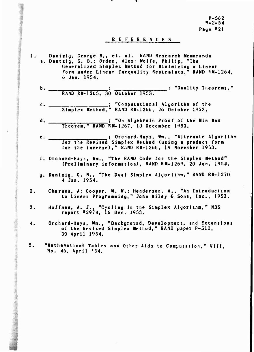
R E F ERE N C E S

Dantzig, George B., et. al. RAND Research Memoranda a. Dantzig, G. B.; Orden, Alex; Wolfe, Philip, "The

Generalized Simplex Method for Minimizing a Linear Form under Linear Inequality Restraints," RAND RM-1264, 6 Jan. 1954.

b. .-.— • 'Duality Theorems," RAND RM.1265, 30 October 1953.

c.

d.

; ^Computational Algorithm of the Simplex Method,** RAND RM-1266, 26 October 1953.

; "On Algebraic Proof of the Min Max Theorem," RAND RM-1267, 10 December 1953.

e. ; Orchard-Hays, Wm., "Alternate Algorithm for the Revised SimpJex Method (using a product form for the inverse)," RAND RM-1266, 19 November 1953.

f. Orchard-Hays, Wm., "The RAND Code for the Simplex Method" (Preliminary information), RAND RM-1269, 20 Jan. 1954.

g. Dantzig, G. B., "The Dual Simplex Algorithm," RAND RM-1270 4 Jan. 1954.

t 2. Chimes, A; Cooper, N. W.; Henderson, A., "An Introduction

to Linear Programming," John Wiley £ Sons, Inc., 1953.

3. Hoffmaa, A. J., "Cycling in the Simplex Algorithm," NBS report »2974, 16 Dec. 1953.

4. Orchard-Hays, Wm., "Background, Development, and Extensions of the Revised Simplex Method," RAND paper P-51Ü, 30 April 1954.

5. "Mathematical Tables and Other Aids to Computation," VIII, No. 46, April '54.