Classnotes - MA1101

Functions of Several Variables

Arindama SinghDepartment of Mathematics

Indian Institute of Technology Madras

Contents

1 Differential Calculus 41.1 Regions in the plane . . . . . . . . . . . . . . . . . . . . . . . . . . . . . . . . . . 41.2 Level curves and surfaces . . . . . . . . . . . . . . . . . . . . . . . . . . . . . . . 51.3 Continuity . . . . . . . . . . . . . . . . . . . . . . . . . . . . . . . . . . . . . . . 101.4 Partial Derivatives . . . . . . . . . . . . . . . . . . . . . . . . . . . . . . . . . . . 121.5 Increment Theorem . . . . . . . . . . . . . . . . . . . . . . . . . . . . . . . . . . 151.6 Chain Rules . . . . . . . . . . . . . . . . . . . . . . . . . . . . . . . . . . . . . . 181.7 Directional Derivative . . . . . . . . . . . . . . . . . . . . . . . . . . . . . . . . . 211.8 Normal to Level Curve and Tangent Planes . . . . . . . . . . . . . . . . . . . . . 241.9 Taylor’s Theorem . . . . . . . . . . . . . . . . . . . . . . . . . . . . . . . . . . . 261.10 Extreme Values . . . . . . . . . . . . . . . . . . . . . . . . . . . . . . . . . . . . 291.11 Lagrange Multipliers . . . . . . . . . . . . . . . . . . . . . . . . . . . . . . . . . 341.12 Review Problems . . . . . . . . . . . . . . . . . . . . . . . . . . . . . . . . . . . 36

2 Multiple Integrals 402.1 Volume of a solid of revolution . . . . . . . . . . . . . . . . . . . . . . . . . . . . 402.2 The Cylindrical Shell Method . . . . . . . . . . . . . . . . . . . . . . . . . . . . 442.3 Approximating Volume . . . . . . . . . . . . . . . . . . . . . . . . . . . . . . . . 462.4 Riemann Sum in Polar coordinates . . . . . . . . . . . . . . . . . . . . . . . . . . 512.5 Triple Integral . . . . . . . . . . . . . . . . . . . . . . . . . . . . . . . . . . . . . 552.6 Triple Integral in Cylindrical coordinates . . . . . . . . . . . . . . . . . . . . . . . 582.7 Triple Integral in Spherical coordinates . . . . . . . . . . . . . . . . . . . . . . . 602.8 Change of Variables . . . . . . . . . . . . . . . . . . . . . . . . . . . . . . . . . . 622.9 Review Problems . . . . . . . . . . . . . . . . . . . . . . . . . . . . . . . . . . . 66

3 Vector Integrals 743.1 Line Integral . . . . . . . . . . . . . . . . . . . . . . . . . . . . . . . . . . . . . 743.2 Line Integral of Vector Fields . . . . . . . . . . . . . . . . . . . . . . . . . . . . . 783.3 Conservative Fields . . . . . . . . . . . . . . . . . . . . . . . . . . . . . . . . . . 793.4 Green’s Theorem . . . . . . . . . . . . . . . . . . . . . . . . . . . . . . . . . . . 843.5 Curl and Divergence of a vector field . . . . . . . . . . . . . . . . . . . . . . . . . 893.6 Surface Area of solids of Revolution . . . . . . . . . . . . . . . . . . . . . . . . . 913.7 Surface area . . . . . . . . . . . . . . . . . . . . . . . . . . . . . . . . . . . . . . 943.8 Integrating over a surface . . . . . . . . . . . . . . . . . . . . . . . . . . . . . . . 99

2

3.9 Surface Integral of a Vector Field . . . . . . . . . . . . . . . . . . . . . . . . . . . 1033.10 Stokes’ Theorem . . . . . . . . . . . . . . . . . . . . . . . . . . . . . . . . . . . 1063.11 Gauss’ Divergence Theorem . . . . . . . . . . . . . . . . . . . . . . . . . . . . . 1113.12 Review Problems . . . . . . . . . . . . . . . . . . . . . . . . . . . . . . . . . . . 115

Bibliography 120

Appendix A One Variable Summary 121A.1 Graphs of Functions . . . . . . . . . . . . . . . . . . . . . . . . . . . . . . . . . . 121A.2 Concepts and Facts . . . . . . . . . . . . . . . . . . . . . . . . . . . . . . . . . . 126A.3 Formulas . . . . . . . . . . . . . . . . . . . . . . . . . . . . . . . . . . . . . . . 133

Index 138

3

Chapter 1

Differential Calculus

1.1 Regions in the planeLet D be a subset of the plane R2 and let (a, b) ∈ R2 be any point.An ε-disk around (a, b) is the set of all points (x, y) ∈ R2 whose distance from (a, b) is less than ε .(a, b) is an interior point of D iff some ε-disk around (a, b) is contained in D.

(a, b) ∈ D is an isolated point of D iff (a, b) is the only point of D that is contained in some ε-diskaround (a, b).(a, b) is a boundary point of D iff every ε-disk around (a, b) contains points from D and pointsnot from D.

R is an open subset of R2 iff all points of D are its interior points.D is a closed subset of R2 iff it contains all its boundary points.D = D∪ the set of boundary points of D; It is the closure of D.

D is a bounded subset of R2 iff D is contained in some ε-disk. (around some point)

An interior point A boundary point

4

D is called a iff it contains all its interior points, possibly some of its boundary points, and satisfiesthe property of connectedness that any two points in D can be joined by a polygonal line entirelylying in D. A region is sometimes called a domain.

Let D be a region in the plane. Let f : D → R be a function.The graph of f is {(x, y, z) ∈ R3 : z = f (x, y), (x, y) ∈ D}.The graph here is also called the surface z = f (x, y).The domain of f is D.The co-domain of f is R.The range of f is {z ∈ R : z = f (x, y) for some (x, y) ∈ D}.

Sometimes, we do not fix the domain D of f but ask you to find it.

The function f (x, y) =√y − x2

has domain D = {(x, y) : x2 ≤ y}.

Its range is the set of all non-negative reals.What is its graph?Some examples of surfaces are here:

1.2 Level curves and surfacesLet f (x, y) be a function of two variables. That is, f : D → R, where D is a region in R2.

A contour curve of f is the curve of intersection of the surface z = f (x, y) and the plane z = c forsome constant c in the range of f . It is the curve f (x, y) = c for some constant c in the range of f .The union of all contour curves is the surface z = f (x, y); it is also the graph of f .

5

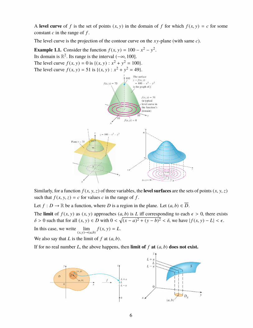
A level curve of f is the set of points (x, y) in the domain of f for which f (x, y) = c for someconstant c in the range of f .

The level curve is the projection of the contour curve on the xy-plane (with same c).

Example 1.1. Consider the function f (x, y) = 100 − x2 − y2.

Its domain is R2. Its range is the interval (−∞, 100].The level curve f (x, y) = 0 is {(x, y) : x2 + y2 = 100}.The level curve f (x, y) = 51 is {(x, y) : x2 + y2 = 49}.

Similarly, for a function f (x, y, z) of three variables, the level surfaces are the sets of points (x, y, z)such that f (x, y, z) = c for values c in the range of f .

Let f : D → R be a function, where D is a region in the plane. Let (a, b) ∈ D.

The limit of f (x, y) as (x, y) approaches (a, b) is L iff corresponding to each ε > 0, there existsδ > 0 such that for all (x, y) ∈ D with 0 <

√(x − a)2 + (y − b)2 < δ, we have | f (x, y) − L | < ε.

In this case, we write lim(x,y)→(a,b)

f (x, y) = L.

We also say that L is the limit of f at (a, b).

If for no real number L, the above happens, then limit of f at (a, b) does not exist.

6

The intuitive understanding of the notion of limit is as follows:The distance between f (x, y) and L can be made arbitrarily small by making the distance between(x, y) and (a, b) sufficiently small but not necessarily zero.It is often difficult to show that limit of a function does not exist at a point. We will come back tothis question soon. When limit exists, we write it in many alternative ways:

The limit of f (x, y) as (x, y) approaches (a, b) is L.

f (x, y) → L as (x, y) → (a, b).

lim(x,y)→(a,b)

f (x, y) = L.

limx→ay→b

f (x, y) = L.

Example 1.2. Determine if lim(x,y)→(0,0)

4xy2

x2 + y2 exists.

Observe that the region D of f is R2 \ {(0, 0)}. And f (0, y) = 0 for y , 0; f (x, 0) = 0 for x , 0.We guess that if the limit exists, it would be 0. To see that it is the case, we start with any ε > 0.We want to choose a δ > 0 such that the following sentence becomes true:

If 0 <√

x2 + y2 < δ, then ���4xy2

x2 + y2��� < ε.

Since |y2 | = y2 ≤ x2 + y2 and |x2 | = x2 ≤ x2 + y2, we have

�����4xy2

x2 + y2

�����≤ 4|x | ≤ 4

√x2 + y2.

So, we choose δ = ε/4. Let us verify whether our choice is all right.Assume that 0 <

√x2 + y2 < δ. Then

�����4xy2

x2 + y2 − 0�����≤ 4

√x2 + y2 < 4δ = ε .

Hencelim

(x,y)→(0,0)

4xy2

x2 + y2 = 0.

Observation: Suppose we have obtained a δ corresponding to some ε . If we take ε1 which islarger than the earlier ε , then the same δ will satisfy the requirement in the definition of the limit.Thus while showing that the limit of a function is such and such at a point, we are free to choose apre-assigned upper bound for our ε .

Similarly, suppose for some ε , we have already obtained a δ such that the limit requirement issatisfied. If we choose another δ, say δ1, which is smaller than δ, then the limit requirement is alsosatisfied. Thus, we are free to choose a pre-assigned upper bound for our δ provided it is convenientto us and it works.

Example 1.3. Consider f (x, y) =√

1 − x2 − y2 where D = {(x, y) : x2 + y2 ≤ 1}.We guess that limit f (x, y) is 1 as (x, y) → (0, 0).

7

To show that the guess is right, let ε > 0. Observe that 0 ≤ f (x, y) ≤ 1 on D.Using our observation, assume that 0 < ε < 1. Choose δ =

√1 − (1 − ε )2. Let |(x, y) − (0, 0) | < δ.

Then 0 < x2 + y2 < 1 − (1 − ε )2 ⇒ 1 − x2 − y2 > (1 − ε )2 ⇒ f (x, y) > 1 − ε .That is, | f (x, y) − 1| = 1 − f (x, y) < ε. Therefore, f (x, y) → 1 as (x, y) → (0, 0).

Theorem 1.1. (Uniqueness of limit) Let f (x, y) be a real valued function defined on a regionD ⊆ R2. Let (a, b) ∈ D. If limit of f (x, y) as (x, y) approaches (a, b) exists, then it is unique.

Proof: Suppose f (x, y) → ` and also f (x, y) → m as (x, y) → (a, b). Let ε > 0. For ε/2, we haveδ1 > 0, δ2 > 0 such that

0 < (x−a)2+(y−b)2 < δ21 ⇒ | f (x, y)−` | < ε/2, 0 < (x−a)2+(y−b)2 < δ2

2 ⇒ | f (x, y)−m | < ε/2.

Choose a point (α, β) so that both 0 < (α − a)2 + (β − b)2 < δ21, 0 < (α − a)2 + (β − b)2 < δ2

2hold. Then

| f (α, β) − ` | < ε/2 and | f (α, β) − m | < ε/2.

Now, |` − m | ≤ |` − f (α, β) | + | f (α, β) − m | < ε/2 + ε/2 = ε . That is, for each ε > 0, we have|` − m | < ε . Hence ` = m. �

For a function of one variable, there are only two directions for approaching a point; from leftand from right. Whereas for a function of two variables, there are infinitely many directions, andinfinite number of paths on which one can approach a point. The limit refers only to the distancebetween (x, y) and (a, b). It does not refer to any specific direction of approach to (a, b). If the limitexists, then f (x, y) must approach the same limit no matter how (x, y) approaches (a, b). Thus, ifwe can find two different paths of approach along which the function f (x, y) has different limits,then it follows that limit of f (x, y) as (x, y) approaches (a, b) does not exist.

Theorem 1.2. Suppose that f (x, y) → L1 as (x, y) → (a, b) along a path C1 and f (x, y) → L2as (x, y) → (a, b) along a path C2. If L1 , L2, then the limit of f (x, y) as (x, y) → (a, b) does notexist.

Example 1.4. Consider f (x, y) =x2 − y2

x2 + y2 for (x, y) , (0, 0).What is its limit at (0, 0)?

When y = 0, limit of f (x, y) as x → 0 is limx→0

x2

x2 = limx→0

(1) = 1.

That is, f (x, y) → 1 as (x, y) → (0, 0) along the x-axis.

When x = 0, limit of f (x, y) as y → 0 is limy→0

−y2

y2 = −1.

That is, f (x, y) → −1 as (x, y) → (0, 0) along the y-axis.Hence lim

(x,y)→(0,0)f (x, y) does not exist.

8

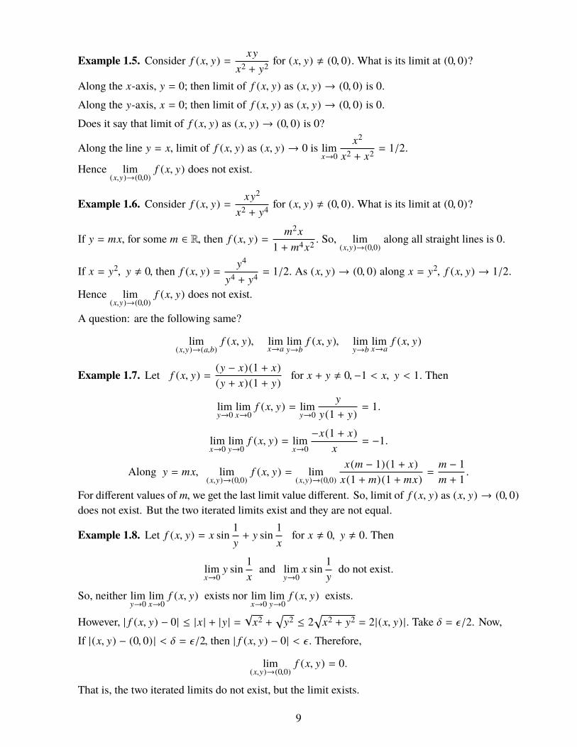
Example 1.5. Consider f (x, y) =xy

x2 + y2 for (x, y) , (0, 0).What is its limit at (0, 0)?

Along the x-axis, y = 0; then limit of f (x, y) as (x, y) → (0, 0) is 0.Along the y-axis, x = 0; then limit of f (x, y) as (x, y) → (0, 0) is 0.Does it say that limit of f (x, y) as (x, y) → (0, 0) is 0?

Along the line y = x, limit of f (x, y) as (x, y) → 0 is limx→0

x2

x2 + x2 = 1/2.

Hence lim(x,y)→(0,0)

f (x, y) does not exist.

Example 1.6. Consider f (x, y) =xy2

x2 + y4 for (x, y) , (0, 0).What is its limit at (0, 0)?

If y = mx, for some m ∈ R, then f (x, y) =m2x

1 + m4x2 . So, lim(x,y)→(0,0)

along all straight lines is 0.

If x = y2, y , 0, then f (x, y) =y4

y4 + y4 = 1/2. As (x, y) → (0, 0) along x = y2, f (x, y) → 1/2.

Hence lim(x,y)→(0,0)

f (x, y) does not exist.

A question: are the following same?

lim(x,y)→(a,b)

f (x, y), limx→a

limy→b

f (x, y), limy→b

limx→a

f (x, y)

Example 1.7. Let f (x, y) =(y − x)(1 + x)(y + x)(1 + y)

for x + y , 0,−1 < x, y < 1. Then

limy→0

limx→0

f (x, y) = limy→0

y

y(1 + y)= 1.

limx→0

limy→0

f (x, y) = limx→0

−x(1 + x)x

= −1.

Along y = mx, lim(x,y)→(0,0)

f (x, y) = lim(x,y)→(0,0)

x(m − 1)(1 + x)x(1 + m)(1 + mx)

=m − 1m + 1

.

For different values of m, we get the last limit value different. So, limit of f (x, y) as (x, y) → (0, 0)does not exist. But the two iterated limits exist and they are not equal.

Example 1.8. Let f (x, y) = x sin1y+ y sin

1x

for x , 0, y , 0. Then

limx→0

y sin1x

and limy→0

x sin1y

do not exist.

So, neither limy→0

limx→0

f (x, y) exists nor limx→0

limy→0

f (x, y) exists.

However, | f (x, y) − 0| ≤ |x | + |y | =√

x2 +√y2 ≤ 2

√x2 + y2 = 2|(x, y) |. Take δ = ε/2. Now,

If |(x, y) − (0, 0) | < δ = ε/2, then | f (x, y) − 0| < ε. Therefore,

lim(x,y)→(0,0)

f (x, y) = 0.

That is, the two iterated limits do not exist, but the limit exists.

9

Hence existence of the limit of f (x, y) as (x, y) → (a, b) and the two iterated limits have noconnection.

The usual operations of addition, multiplication etc have the expected effects as the followingtheorem shows. Its proof is analogous to the single variable limits.

Theorem 1.3. Let L, M, c ∈ R; lim(x,y)→(a,b)

f (x, y) = L; lim(x,y)→(a,b)

g(x, y) = M . Then

1. Constant Multiple : lim(x,y)→(a,b)

c f (x, y) = cL.

2. Sum : lim(x,y)→(a,b)

( f (x, y) + g(x, y)) = L + M .

3. Product : lim(x,y)→(a,b)

( f (x, y) g(x, y)) = LM .

4. Quotient : If M , 0 and g(x, y) , 0 in an open disk around the point (a, b), thenlim

(x,y)→(a,b)( f (x, y)/g(x, y)) = L/M

5. Power : If r ∈ R, Lr ∈ R and lim(x,y)→(a,b)

f (x, y) = L, then lim(x,y)→(a,b)

( f (x, y))r = Lr .

1.3 ContinuityLet f (x, y) be a real valued function defined on a subsets D ofR2.We say that f (x, y) is continuousat a point (a, b) ∈ D iff for each ε > 0, there exists δ > 0 such that for all points (x, y) ∈ D with√

(x − a)2 + (y − b)2 < δ we have | f (x, y) − f (a, b) | < ε .Observe that if (a, b) is an isolated point of D, then f is continuous at (a, b). When D is a region,(a, b) is not an isolated point of D; and then f is continuous at (a, b) ∈ D iff the following aresatisfied:

1. f (a, b) is well defined, that is, (a, b) ∈ D;

2. lim(x,y)→(a,b)

f (x, y) exists; and

3. lim(x,y)→(a,b)

f (x, y) = f (a, b).

The function f (x, y) is said to be continuous on a subset of D iff f (x, y) is continuous at all pointsin the subset.Therefore, constant multiples, sum, difference, product, quotient, and rational powers of continuousfunctions are continuous whenever they are well defined.Polynomials in two variables are continuous functions.Rational functions, i.e., ratios of polynomials, are continuous functions provided they are welldefined.

Example 1.9. f (x, y) =

3x2yx2+y2 if (x, y) , (0, 0)

0 if (x, y) = (0, 0)is continuous on R2.

10

At any point other than the origin, f (x, y) is a rational function; therefore, it is continuous. Tosee that f (x, y) is continuous at the origin, let ε > 0 be given. Take δ = ε/3. Assume that√

x2 + y2 < δ. Then

���3x2y

x2 + y2 − f (0, 0)��� ≤���3(x2 + y2)y

x2 + y2��� ≤ 3|y | ≤ 3

√x2 + y2 < 3δ = ε .

Example 1.10. f (x, y) =

xy(x2−y2)x2+y2 if (x, y) , (0, 0)

0 if (x, y) = (0, 0)is continuous on R2.Why?

Being a rational function, it is continuous at all nonzero points. For the point (0, 0), let ε > 0 begiven. Choose δ =

√ε . Notice that xy ≤ x2 + y2 and x2 − y2 ≤ x2 + y2.

For all (x, y) with√

x2 + y2 < δ, we have

| f (x, y) − 0| ≤(x2 + y2)(x2 + y2)

x2 + y2 < δ2 = ε .

Hence lim(x,y)→(0,0)

f (x, y) = 0 = f (0, 0).

Example 1.11. f (x, y) =x2 − y2

x2 + y2 is continuous on D = R2 \ {(0, 0)}.

f (x, y) is not continuous at (0, 0) since (0, 0) < D.

What about the function g(x, y), where

g(x, y) =

x2−y2

x2+y2 if (x, y) , (0, 0)

0 if (x, y) = (0, 0)

By Example 1.4, lim(x,y)→(0,0)

g(x, y) does not exist. Hence g(x, y) is not continuous at (0, 0).

As in the single variable case, composition of continuous functions is continuous:

Let f : D → R be continuous at (a, b) with f (a, b) = c. Let g : I → R be continuousat c ∈ I for some interval I in R. Then g( f (x, y)) from D to R is continuous at (a, b).

Proof of this fact is left to you as an exercise.For example,

ex−y is continuous at all points in the plane.

cosxy

1 + x2 and ln(1 + x2 + y2) are continuous on R2.

At which points is tan−1(y/x) continuous?Well, the function y/x is continuous everywhere except when x = 0.The function tan−1 is continuous everywhere on R.So, tan−1(y/x) is continuous everywhere except when x = 0.The function (x2 + y2 + z2 − 1)−1 is continuous everywhere except on the sphere x2 + y2 + z2 = 1,where it is not defined.

11

1.4 Partial DerivativesLet f (x, y) be a real valued function defined on a region D ⊆ R2. Let (a, b) ∈ D.

If C is the curve of intersection of the surface z = f (x, y) with the plane y = b, then the slope ofthe tangent line to C at (a, b, f (a, b)) is the partial derivative of f (x, y) with respect to x at (a, b).In the figure take x0 = a, y0 = b. A formal definition of the partial derivative follows.The partial derivative of f (x, y) with respect to x at the point (a, b) is

f x (a, b) =∂ f∂x

���(a,b)=

df (x, b)dx

���x=a= lim

h→0

f (a + h, b) − f (a, b)h

,

provided this limit exists. Notice that f (x, b) must be continuous at x = a.The partial derivative of f (x, y) with respect to y at the point (a, b) is

f y (a, b) =∂ f∂y

���(a,b)=

df (a, y)dy

���y=b= lim

k→0

f (a, b + k) − f (a, b)k

,

provided this limit exists. Again, f (a, y) must be continuous at y = b.

Example 1.12. Find f x (1, 1) where f (x, y) = 4 − x2 − 2y2.

f x (1, 1) = limh→0

(4 − (1 + h)2 − 2) − (4 − 1 − 2)h

= limh→0

−2h − h2

h= −2.

That is, treat y as a constant and differentiate with respect to x.

f x (1, 1) = f x (x, y)��(1,1) = −2x��(1,1) = −2.

12

The vertical plane y = 1 crosses the paraboloid in the curve C1 : z = 2 − x2, y = 1. The slopeof the tangent line to this parabola at the point (1, 1, 1) (which corresponds to (x, y) = (1, 1)) isf x (1, 1) = −2.

Example 1.13. Find f x and f y, where f (x, y) = y sin(xy).

Treating y as a constant and differentiating with respect to x, we get f x . Similarly, f y .

f x (x, y) = y cos(xy) y, f y (x, y) = yx cos(xy) + sin(xy).

Example 1.14. Find ∂z/∂x and ∂z/∂y where z = f (x, y) is defined by x3 + y3 + z3 − 6xyz = 1.

Differentiate x3 + y3 + z3 − 6xyz − 1 = 0 with respect to x treating y as a constant:

3x2 + 0 + 3z2 ∂z∂x− 6y

(z + x

∂z∂x

)− 0 = 0.

Solving this for ∂z/∂x, we have

∂z∂x

(3z2 − 6xy) + (3x2 − 6yz) = 0, that is,

∂z∂x= −

x2 − 2yzz2 − 2xy

.

Similarly,∂z∂y= −

y2 − 2xzz2 − 2xy

.

Example 1.15. The plane x = 1 intersects the surface z = x2 + y2 in a parabola. Find the slope ofthe tangent to the parabola at the point (1, 2, 5).

The asked slope is ∂z/∂y at (1, 2). It is

∂(x2 + y2)∂y

(1, 2) = (2y)(1, 2) = 4.

Alternatively, the parabola is z = x2 + y2, x = 1 OR, z = 1 + y2. So, the slope at (1, 2, 5) is

dzdy

���y=2=

d(1 + y2)dy

���y=2= (2y) |y=2 = 4.

For a function f (x, y), partial derivatives of second order are:

f xx = ( f x)x =∂

∂x∂ f∂x=∂2 f∂x2 .

f xy = ( f x)y =∂ f x

∂y=

∂

∂y

∂ f∂x=

∂2 f∂y∂x

.

f yx = ( f y)x =∂ f y∂x=

∂

∂x∂ f∂y=

∂2 f∂x∂y

.

f yy = ( f y)y =∂

∂y

∂ f∂y=∂2 f∂y2 .

13

Similarly, higher order partial derivatives are defined. For example,

f xxy =∂

∂y

∂

∂x∂ f∂x=

∂3 f∂y∂x∂x

.

Observe that f x (a, b) is not the same as lim(x,y)→(a,b)

f x (x, y). To see this, let

f (x, y) =

1 if x > 00 if x ≤ 0.

Then f x (x, y) = 0 for all x > 0. Also, f x (x, y) = 0 for all x < 0. Now, lim(x,y)→(0,0)

f x (x, y) = 0. But

f x (0, 0) does not exist. Reason?

f x (0, 0) = limh→0

f (h, 0) − f (0, 0)h

= limh→0

1 or 0h

does not exist

On the other hand, f x (a, b) can exist though lim(x,y)→(a,b)

f x does not.

However, if f x (x, y) is continuous at (a, b), then

f x (a, b) = lim(x,y)→(a,b)

f x (x, y).

Similarly, f xy need not be equal to f yx . See the following example.

Example 1.16. Consider f (x, y) =xy(x2 − y2)

x2 + y2 for (x, y) , (0, 0), and f (0, 0) = 0.

f (x, 0) = f (0, y) = f (0, 0) = 0.f x (x, 0) = f y (0, y) = f xx (0, 0) = f yy (0, 0) = 0.

f x (0, y) = limh→0

f (h, y) − f (0, y)h

= −y, f y (x, 0) = limk→0

f (x, k) − f (x, 0)k

= x.

f xy (0, 0) = limk→0

f x (0, k) − f x (0, 0)k

= limk→0

−k − 0k

= −1.

f yx (0, 0) = limh→0

f y (h, 0) − f y (0, 0)h

= limh→0

h − 0h= 1.

That is, f xy , f yx .

But continuity of both of f xy and f yx implies their equality.

Theorem 1.4. (Clairaut) Let D be a region in R2. Let the function f : D → R have continuousfirst and second order partial derivatives on D. Then f xy = f yx .

Proof: Let (a, b) ∈ D. Let h , 0.Write g(x) = f (x, b + h) − f (x, b). Then

φ( f ) := g(a + h) − g(a) = [ f (a + h, b + h) − f (a + h, b)] − [ f (a, b + h) − f (a, b)].

14

By MVT, we have c between a and a + h such that

φ( f ) = g′(c)h = h[ f x (c, b + h) − f x (c, b)].

Again, by MVT (on f x with the second variable), we have d between b and b + h such that

φ( f ) = h · h · f xy (c, d) = h2 f xy (c, d).

Due to continuity of f xy, we have

limh→0

φ( f )h2 = lim

(c,d)→(a,b)f xy (c, d) = f xy (a, b).

Writeφ( f ) = [ f (a + h, b + h) − f (a, b + h)] − [ f (a + h, b) − f (a, b)]

and apply MVT twice as above to get f yx (a, b) = limh→0φ( f )

h2 . But the two limits withφ( f )/h2 are equal. So, f xy (a, b) = f yx (a, b). �

In one variable, f ′(t) exists at t = a implies that f (t) is continuous at t = a.We have seen similarlythat existence of f x (a, b) and f y (a, b) guarantees continuity of f (x, b) and of f (a, y) at (a, b).But for f (x, y), even both f x (x, y) and f y (x, y) exist at (a, b), the function f (x, y) need not becontinuous at (a, b). See the following example.

Example 1.17. Let f (x, y) =

xyx2+y2 if (x, y) , (0, 0)

0 if (x, y) = (0, 0).

Here, f (x, 0) = 0 = f (0, y). So, f x (0, 0) = 0 = f y (0, 0). And limit of f (x, y) as (x, y) → (0, 0)does not exist. Hence f (x, y) is not continuous at (0, 0).

Further, we find that f xx (x, 0) = 0 = f yy (0, y).What about f xy (0, 0)?

f x (0, y) = limh→0

f (h, y) − f (0, y)h

= limh→0

y

h2 + y2 =1y.

f x (0, y) is not continuous at y = 0.Notice that the second partial derivatives f xy (0, 0) and f yx (0, 0) do not exist.

1.5 Increment TheoremIn order to see the connection between continuity of a function and the partial derivatives, theassociated geometry may help.

Let S be the surface z = f (x, y), where f x, f y are continuous on the region D, the domain of f . Let(a, b) ∈ D. Let C1 and C2 be the curves of intersection of the planes x = a and of y = b with S.

15

Let T1 and T2 be tangent lines to the curves C1 and C2 at the point P(a, b, f (a, b)). The tangentplane to the surface S at P is the plane containing T1 and T2.

The tangent plane to S at P consists of all possible tangent lines at P to the curves C that lie on Sand pass through P. This plane approximates S at P most closely.Write the z-coordinate of P as c. Then P = (a, b, c). Equation of any plane passing through P isz− c = A(x− a)+ B(y− b).When y = b, the tangent plane represents the tangent to the intersectedcurve at P. Thus, A = f x (a, b), the slope of the tangent line. Similarly, B = f y (a, b). Henceequation of the tangent plane to the surface z = f (x, y) at the point P(a, b, c) on S is

z − c = f x (a, b)(x − a) + f y (a, b)(y − b)

provided that f x, f y are continuous at (a, b).

Example 1.18. Find the equation of the tangent plane to the elliptic paraboloid z = 2x2 + y2 at(1, 1, 3).

Here, zx = 4x, zy = 2y. So, zx (1, 1) = 4, zy (1, 1) = 2. Then the equation of the tangent plane isz − 3 = 4(x − 1) + 2(y − 1). It simplifies to z = 4x + 2y − 3.The tangent plane gives a linear approximation to the surface at that point. Why?Write the equation as f (x, y) − f (a, b) = f x (a, b)(x − a) + f y (a, b)(y − b). Then

f (x, y) = f (a, b) + f x (a, b)(x − a) + f y (a, b)(y − b).

This formula holds true for all points (x, y, f (x, y)) on the tangent plane at (a, b, f (a, b)). Forapproximating f (x, y) for (x, y) close to (a, b), we may take

f (x, y) ≈ f (a, b) + f x (a, b)(x − a) + f y (a, b)(y − b).

The RHS is called the standard linear approximation of f (x, y, z).Writing in the increment form,

f (a + h, b + k) ≈ f (a, b) + f x (a, b)h + f y (a, b)k .

This gives rise to the total increment f (a + h, b + k) − f (a, b).

The total increment can be written in a more suggestive form. Towards this, write

∆ f := f (a + h, b + k) − f (a + h, b) + f (a + h, b) − f (a, b).

16

By MVT, there exist c ∈ [a, a + h] and d ∈ [b, b + k] such that

f (a + h, b) − f (a, b) = h[ f x (c, b) − f x (a, b)] + h f x (a, b)

f (a + h, b + k) − f (a + h, b) = k[ f y (a + h, d) − f y (a, b)] + k f y (a, b)

Write ε1 = f x (d, b) − f x (a, b) and ε2 = f y (a + h, c) − f y (a, b).When both h → 0, k → 0, we seethat c → a and d → b. Since f x and f y are assumed to be continuous, we have ε1 → 0 and ε2 → 0.Then the total increment can be written as

∆ f = f (a + h, b + k) − f (a, b) = h f x (a, b) + k f y (a, b) + ε1h + ε2k,

where ε1 → 0 and ε2 → 0 as both h → 0, k → 0.We also write the increments h, k in x, y as ∆x, ∆y respectively.From the above rewriting of ∆ f it is also clear that f (x, y) is a continuous function. Let us notedown what we have proved.

Theorem 1.5. (Increment Theorem) Let D be a region in R2. Let the function f : D → R havecontinuous first order partial derivatives on D. Then f (x, y) is continuous on D and the totalincrement ∆ f = f (a + ∆x, b + ∆y) − f (a, b) at (a, b) ∈ D can be written as

∆ f = f x (a, b)∆x + f y∆y + ε1∆x + ε2∆y,

where ε1 → 0 and ε2 → 0 as both ∆x → 0 and ∆y → 0.

Recall that for a function g of one variable, its differential is defined as dg = g′(t)dt.

Let f (x, y) be a given function. The differential of f , also called the total differential, is

df = f x (x, y)dx + f y (x, y)dy.

Here, dx = ∆x and dy = ∆y are the increments in x and y, respectively. Then df is a linearapproximation to the total increment ∆ f .

Example 1.19. The dimensions of a rectangular box are measured to be 75cm, 60cm, and 40 cm,and each measurement is correct to within 0.2cm. Use differentials to estimate the largest possibleerror when the volume of the box is calculated from these measurements.

The volume of the box is V = xyz. So,

dV =∂V∂x

dx +∂V∂y

dy +∂V∂z

dz.

Given that |∆x |, |∆y |, |∆z | ≤ 0.2cm, the largest error in cubic cm is

|∆V | ≈ |dV | = 60 × 40 × 0.2 + 40 × 75 × 0.2 + 75 × 60 × 0.2 = 1980.

Notice that the relative error is 1980/(75 × 60 × 40) which is about 1%.

17

Remark: Let D be a region in R2. A function f : D → R is called differentiable at a point(a, b) ∈ D if the total increment ∆z = f (a + ∆x, b + ∆y) − f (a, b) in f with respect to increments∆x,∆y in x, y, can be written as

∆z = f x (a, b)∆x + f y (a, b)∆y + ε1∆x + ε2∆y

where ε1 → 0 and ε2 → 0 as both ∆x → 0 and ∆y → 0.The following statements give some connections between differentiability, continuity and the partialderivatives.

• Let D be a region in R2. Let f : D → R be such that both f x and f y exist on D and at leastone of them is continuous at (a, b) ∈ D. Then f is differentiable at (a, b).

• Let D be a region in R2. Let f : D → R be differentiable at (a, b) ∈ D. Then f is continuousat (a, b).

Notice that the first statement strengthens the increment theorem. Instead of increasing the loadon terminology, we will continue with the increment theorem. Note that whenever we assumethat f x and f y are continuous, you may replace this with the weaker assumption: “ f (x, y) isdifferentiable”.Remember that we formulate and discuss our results for a function f (x, y) of two variables.Analogously, all the notions and the results can be formulated for a function f (x1, . . . , xn) of nvariables for n ≥ 2.

1.6 Chain RulesWe apply the increment theorem to partially differentiate composite functions.

Theorem 1.6. (Chain Rule 1) Let x(t) and y(t) be differentiable functions. Let f (x, y) havecontinuous first order partial derivatives. Then

dfdt=∂ f∂x

dxdt+∂ f∂y

dydt.

Proof: Using the increment theorem (Theorem 1.5) at a point P we obtain

∆ f∆t=∂ f∂x∆x∆t+∂ f∂y

∆y

∆t+ ε1∆x∆t+ ε2∆y

∆t.

As ∆t → 0, we have ∆x → 0,∆y → 0, ε1 → 0, ε2 → 0. Then the result follows. �

For example, if z = xy and x = sin t, y = cos t, then

dzdt=∂z∂x

x′(t) +∂z∂y

y′(t) = cos2 t − sin2 t .

Check: z(t) = sin t cos t = 12 sin 2t. So, z′(t) = cos 2t = cos2 t − sin2 t.

18

Theorem 1.7. (Chain Rule 2) Let f (x, y) have continuous first order partial derivatives. Supposex = x(s, t) and y = y(s, t) are functions such that xs, xt, ys and yt are also continuous. Then

∂ f∂s=∂ f∂x

∂x∂s+∂ f∂y

∂y

∂s,

∂ f∂t=∂ f∂x

∂x∂t+∂ f∂y

∂y

∂t.

Proof of this follows a similar line to that of Chain Rule - 1. The pattern is clearer if you use thesubscript notation:

f s = f x xs + f yys, f t = f x xt + f yyt .

Example 1.20. Let z = ex sin y, x = st2, y = s2t. Then

∂z∂s= (ex sin y)t2 + (ex cos y)2st = test2

(t sin(s2t) + 2s cos(s2t)).

∂z∂t= (ex sin y)2st + (ex cos y)s2 = sest2

(2t sin(s2t) + s cos(s2t)).

Substitute expressions for x and y to get z = z(s, t) and then check that the results are correct.

Example 1.21. Given that z = f (x, y) has continuous second order partial derivatives and thatx = r2 + s2, y = 2rs, find zrr .

We have xr = 2r, yr = 2s. Then

zr = 2r zx + 2szy .

zxr = zxx xr + zxyyr = 2r zxx + 2szxy .

zyr = zyx xr + zyyyr = 2r zyx + 2szyy .

zrr =∂zr

∂r=

∂

∂r(2r zx + 2szy) = 2zx + 2r zxr + 2szyr

= 2zx + 2r (2r zxx + 2szxy) + 2s(2r zyx + 2szyy)

= 2zx + 4r2zxx + 8rszxy + 4s2zyy .

Functions can be differentiated implicitly. If F is defined within a sphere S containing a point(a, b, c), where F (a, b, c) = 0, Fz (a, b, c) , 0, and Fx, Fy, Fz are continuous inside the sphere,then the equation F (x, y, z) = 0 defines a function z = f (x, y) in a sphere containing (a, b, c) andcontained in the sphere S. Moreover, the function z = f (x, y) can now be differentiated partiallywith zx = −Fx/Fz, zy = −Fy/Fz .

It is easier to differentiate implicitly than remembering the formula.

Example 1.22. Find zx and zy if x3 + y3 + z3 + 6xyz = 1.

We differentiate ‘the equation’ with respect to x and y as follows:

3x2 + 3z2zx + 6y(z + xzx) = 0⇒ zx = −(x2 + 2yz)z2 + 2xy

.

3y2 + 3z2zy + 6x(z + xzy) = 0⇒ zy = −(y2 + 2xz)z2 + 2xy

.

19

Example 1.23. Find dydx

if y = y(x) is given by y2 = x2 + sin(xy).

2ydydx− 2x − cos(xy)(y + x

dydx

) = 0⇒dydx=

2x + y cos(xy)2y − x cos(xy)

.

Example 1.24. Find wx if w = x2 + y2 + z2 and z = x2 + y2.

As it looks,∂w

∂x= 2x.

However, since z = x2 + y2, we have w = x2 + y2 + (x2 + y2)2. Then

∂w

∂x= 2x + 4x3 + 4xy2.

Notice that, here we take z as the dependent variable and x, y as independent variables. But supposewe know that x and z are the independent variables and y is the dependent variable. Then thesecond equation says that y2 = z − x2. Then w = x2 + (z − x2) + z2 = z + z2. Thus

∂w

∂x= 0.

The correct procedure to get ∂w/∂x is :

1. w must be dependent variable and x must be independent variable.

2. Decide which of the other variables are dependent or independent.

3. Eliminate the dependent variables from w using the constraints.

4. Then take the partial derivative ∂w/∂x.

Example 1.25. Given that w = x2 + y2 + z2 and z(x, y) satisfies z3 − xy + yz + y3 = 1, evaluate∂w/∂x at (2,−1, 1).

It is now clear that z,w are dependent variables and x, y are independent variables. So,

∂w

∂x= 2x + 2z

∂z∂x, 3z2 ∂z

∂x− y + y

∂z∂x= 0.

These two together give ∂w∂x = 2x + 2yz

y+3z2 . Evaluating it at (2,−1, 1) gives ∂w∂x (2,−1, 1) = 3.

A function f (x, y) is called homogeneous of degree n in a region D ⊆ R2 if for all (x, y) ∈ D,and for each positive λ, f (λx, λy) = λn f (x, y).

For example, f (x, y) = x1/3y−4/3 tan−1(y/x) is homogeneous of degree −1 in the region D, whichis any quadrant without the axes.f (x, y) = (

√x2 + y2)3 is homogeneous of degree 3 in the whole plane.

Theorem 1.8. (Euler) Let D be a region in R2. Let f : D → R have continuous first order partialderivatives. Then f is a homogeneous function of degree n iff x f x + y f y = n f .

20

Proof: Differentiate f (λx, λy) − λn f (x, y) = 0 partially with respect to λ to obtain:

x f x (λx, λy) + y f y (λx, λy) = nλn−1 f (x, y).

Then set λ = 1 to get x f x (x, y) + y f y (x, y) = n f (x, y).Conversely, let (a, b) ∈ D. Define φ(λ) = f (λa, λb). Differentiate with respect to λ to get

λφ′(λ) = a f x (λa, λb) + b f y (λa, λb).

However,

n f (λa, λb) = a f x (λa, λb) + b f y (λa, λb) = λa f x (λa, λb) + λb f y (λa, λb).

That is,λφ′(λ) = nφ(λ).

Now, differentiate λ−nφ(λ) with respect to λ to obtain

[φ(λ)λ−n]′ = φ′(λ)λ−n − nφ(λ)λ−n−1 = 0.

Therefore, φ(λ)λ−n = c for some constant c. Set λ = 1 to get c = f (a, b). Then

f (λa, λb) = λn f (a, b).

Since (a, b) is any arbitrary point in D, we have f (λx, λy) = λn f (x, y). �

For our earlier examples, you can check that

x∂[x1/3y−4/3 tan−1(y/x)]

∂x+ y

∂[x1/3y−4/3 tan−1(y/x)]∂y

+ x1/3y−4/3 tan−1(y/x) = 0.

x∂[(

√x2 + y2)3]∂x

+ y∂[(

√x2 + y2)3]∂y

= 3[(√

x2 + y2)3].

1.7 Directional DerivativeRecall that if f (x, y) is a function, then f x (x0, y0) is the rate of change in f with respect to changein x, at (x0, y0), that is, in the direction ı. Similarly, f y (x0, y0) is the rate of change at (x0, y0) inthe direction . How do we find the rate of change of f (x, y) at (x0, y0) in the direction of any unitvector u?

21

Consider the surface S with the equation z = f (x, y). Let z0 = f (x0, y0). The point P(x0, y0, z0)lies on S. The vertical plane that passes through P in the direction of u (containing u) intersects Sin a curve C. The slope of the tangent line T to the curve C at the point P is the rate of change of zin the direction of u.

Let f (x, y) be a function defined in a region D. Let (x0, y0) ∈ D. The directional derivative off (x, y) in the direction of a unit vector u = aı + b at (x0, y0) is given by

(Du f )(x0, y0) =(

dfds

)u

���(x0,y0)= lim

h→0

f (x0 + ha, y0 + hb) − f (x0, y0)h

.

Example 1.26. Find the derivative of z = x2 + y2 at (1, 2) in the direction u = (1/√

2)ı+ (1/√

2) .

Duz(1, 2) = limh→0

f(1 + h/

√2, 2 + h/

√2)− f (1, 2)

h= lim

h→0

2h/√

2 + 2 · 2h/√

2h

=6√

2.

Notice that f x (1, 2)(1/√

2) + f y (1, 2)(1/√

2) = (2 + 2(2)) · (1/√

2) = 6/√

2.

Theorem 1.9. Let f (x, y) have continuous first order partial derivatives. Then f (x, y) has adirectional derivative at (x, y) in any direction u = aı + b ; and it is given by

Du f (x, y) = f x (x, y)a + f y (x, y)b.

Proof: Let (x0, y0) be a point in the domain of definition of f (x, y). Define the function g(·) byg(h) = f (x0 + ah, y0 + bh). Then g(h) is a continuously differentiable function of h. Now,

g′(h) = f xdxdh+ f y

dydh= f x a + f y b.

Then g′(0) = f x (x0, y0) a + f y (x0, y0) b. Also,

g′(0) = limh→0

g(h) − g(0)h

= Du f (x0, y0).

Hence Du f (x0, y0) = g′(0) = f x (x0, y0)a + f y (x0, y0)b. �

Example 1.27. Find the directional derivative of f (x, y) = x3 − 3xy + 4y2 in the direction of theline that makes an angle of π/6 with the x-axis.

Here, the direction is given by the unit vector u = cos(π/6)ı + sin(π/6) =

√3

2ı +

12. Thus

Du f (x, y) =

√3

2f x +

12

f y =

√3

2(3x2 − 3y) +

12

(−3x + 8y) =12

[3√

3x2 − 3x + (8 − 3√

3)y].

The formula for the directional derivative in the direction of the unit vector u = aı + b can bewritten as

Du f = f xa + f yb = ( f x ı + f y ) · (aı + b ).

22

The vector operator ∇ :=∂

∂xı +

∂

∂y is called the gradient and the gradient of f (x, y) is

∇ f := grad f :=∂ f∂xı +

∂ f∂y

.

Therefore, Du f = grad f · u. That is, at (x0, y0), the directional derivative is given by

Du f |(x0,y0) = grad f |(x0,y0) · u.

For example, for the function f (x, y) = xey + cos(xy), grad f |(2,0) = ı + 2 . Thus, the directionalderivative of f in the direction of 3ı − 4 is grad f |(1,2) · ((3/5)ı − (4/5) ) = −1.Caution: To apply this formula, we have assumed that f x, f y are continuous at (x0, y0), and u is aunit vector.

Example 1.28. How much the value of y sin x + 2yz change if the point (x, y, z) moves 0.1 unitsfrom (0, 1, 0) toward (2, 2,−2)?

Let f (x, y, z) = y sin x + 2yz. P(0, 1, 0), Q(2, 2,−2). #»v =# »PQ = 2ı+ − 2k . The unit vector in the

direction of #»v is u = 13

#»v .We find Du at P which requires grad f .

grad f = (y cos x)ı + (sin x + 2z) + 2y k .

ThenDu(P) = grad f |(0,1,0) ·

#»u = (ı + 2k) · u = −23.

The change df in the direction of #»u in moving ds = 0.1 units is approximately

df ≈ Du(P) ds = −23

(0.1) = −0.067 units.

Theorem 1.10. Let f (x, y) have continuous first order partial derivatives. The maximum value ofthe directional derivative Du f (x, y) is |grad f | and it is achieved when the unit vector u has thesame direction as that of grad f .

This is obvious since Du f = grad f · u says that the directional derivative is the scalar projectionof the gradient in the direction of u.

Proof: Du f = grad f · u = |grad f | |u| cos θ = |grad f | cos θ, where θ is the angle between grad fand u. Since maximum of cos θ is 1,maximum of Du f is |grad f |. The maximum is achieved whenθ = 0, that is, when the directions of grad f and u coincide. �

This also says the following:f (x, y) increases most rapidly in the direction of its gradient.f (x, y) decreases most rapidly in the opposite direction of its gradient.f (x, y) remains constant in any direction orthogonal to its gradient.

23

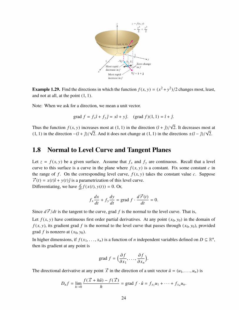
Example 1.29. Find the directions in which the function f (x, y) = (x2+ y2)/2 changes most, least,and not at all, at the point (1, 1).

Note: When we ask for a direction, we mean a unit vector.

grad f = f x ı + f y = xı + y . (grad f )(1, 1) = ı + .

Thus the function f (x, y) increases most at (1, 1) in the direction (ı + )/√

2. It decreases most at(1, 1) in the direction −(ı + )/

√2. And it does not change at (1, 1) in the directions ±(ı − )/

√2.

1.8 Normal to Level Curve and Tangent PlanesLet z = f (x, y) be a given surface. Assume that f x and f y are continuous. Recall that a levelcurve to this surface is a curve in the plane where f (x, y) is a constant. Fix some constant c inthe range of f . On the corresponding level curve, f (x, y) takes the constant value c. Suppose#»r (t) = x(t)ı + y(t) is a parametrization of this level curve.Differentiating, we have d

dt f (x(t), y(t)) = 0. Or,

f xdxdt+ f y

dydt= grad f ·

d #»r (t)dt

= 0.

Since d #»r /dt is the tangent to the curve, grad f is the normal to the level curve. That is,Let f (x, y) have continuous first order partial derivatives. At any point (x0, y0) in the domain off (x, y), its gradient grad f is the normal to the level curve that passes through (x0, y0), providedgrad f is nonzero at (x0, y0).In higher dimensions, if f (x1, . . . , xn) is a function of n independent variables defined on D ⊆ Rn,

then its gradient at any point is

grad f =( ∂ f∂x1

, . . . ,∂ f∂xn

).

The directional derivative at any point #»x in the direction of a unit vector u = (u1, . . . , un) is

Du f = limh→0

f ( #»x + hu) − f ( #»x )h

= grad f · u = f x1u1 + · · · + f xnun.

24

The algebraic rules for the gradient are as follows:1. Constant multiple: grad (k f ) = k (grad f ) for k ∈ R.2. Sum: grad ( f + g) = grad f + grad g.

3. Difference: grad ( f − g) = grad f − grad g.

4. Product: grad ( f g) = f (grad g) + g(grad f ).

5. Quotient: grad ( f /g) =g(grad f ) − f (grad g)

g2 .

In R3, let #»r (t) = x(t)ı + y(t) + z(t) k be a smooth curve on the level surface f (x, y, z) = c. Thenf (x(t), y(t), z(t)) = c for all t. Differentiating this we get

grad f · #»r ′(t) = 0.

Look at all such smooth curves that pass through a point P on the level surface. The velocityvectors #»r ′(t) to all these smooth curves are orthogonal to the gradient at P.

Let f (x, y, z) have continuous partial derivatives f x, f y, and f z . The tangent plane at P(x0, y0, z0)on the level surface f (x, y, z) = c is the plane through P which is orthogonal to grad f at P. Itsequation is

f x (x0, y0, z0)(x − x0) + f y (x0, y0, z0)(y − y0) + f z (x0, y0, z0)(z − z0) = 0.

The normal line to the level surface f (x, y, z) = c at P(x0, y0, z0) is the line through P parallel tograd f . Its parametric equation is

x = x0 + f x (x0, y0, z0) t, y = y0 + f y (x0, y0, z0) t, z = z0 + f z (x0, y0, z0) t.

The equation of the tangent plane to the surface z = f (x, y) at (a, b) can be obtained as follows:Write the surface as F (x, y, z) = 0,where F (x, y, z) = f (x, y)− z. Then Fx = f x, Fy = f y, Fz = −1.Then the equation of the tangent plane is

f x (a, b)(x − a) + f y (a, b)(y − b) − (z − f (a, b)) = 0.

Example 1.30. Find the tangent plane and the normal line of the surface x2 + y2 + z − 9 = 0 at thepoint (1, 2, 4).

First, check that the point (1, 2, 4) lies on the surface. Next, f x (1, 2, 4) = 2, f y (1, 2, 4) = 4 andf z (1, 2, 4) = 1. The tangent plane is given by

2(x − 1) + 4(y − 2) + (z − 4) = 0.

The normal line at (1, 2, 4) is given by

x = 1 + 2t, y = 2 + 4t, z = 4 + t.

Example 1.31. Find the tangent plane to the surface z = x cos y − yex at the origin.

f x (0, 0) = 1, f y (0, 0) = −1. The tangent plane is

x − y − z = 0.

25

Example 1.32. Find the tangent line to the curve of intersection of the surfacesf (x, y, z) := x2 + y2 − 2 = 0 and g(x, y, z) := x + z − 4 = 0 at the point (1, 1, 3).

The tangent line is orthogonal to both grad f and grad g at (1, 1, 3). So, it is parallel to

grad f × grad g = (2ı + 2 ) × (ı + k) = 2ı − 2 − 2k .

Thus the tangent line is x = 1 + 2t, y = 1 − 2t, z = 3 − 2t.

1.9 Taylor’s TheoremFor a function of one variable, a polynomial approximation is given by the Taylor’s formula.Observe that it is a generalization of the Mean value theorem.

Theorem1.11. (Taylor’s Formula for one variable) Let n ∈ N. Suppose that f (n) (x) is continuouson [a, b] and is differentiable on (a, b). Then there exists a point c ∈ (a, b) such that

f (x) = f (a) + f ′(a)(x − a) +f ′′(a)

2!(x − a)2 + · · · +

f (n) (a)n!

(x − a)n +f (n+1) (c)(n + 1)!

(x − a)n+1.

Proof: For x = a, the formula holds. So, let x ∈ (a, b]. For any t ∈ [a, x], let

p(t) = f (a) + f ′(a)(t − a) +f ′′(a)

2!(t − a)2 + · · · +

f (n) (a)n!

(t − a)n.

Here, we treat x as a certain point, not a variable; and t as a variable. Write

g(t) = f (t) − p(t) −f (x) − p(x)(x − a)n+1 (t − a)n+1.

We see that g(a) = 0, g′(a) = 0, g′′(a) = 0, . . . , g(n) (a) = 0, and g(x) = 0.By Rolle’s theorem, there exists c1 ∈ (a, x) such that g′(c1) = 0. Since g(a) = 0, apply Rolle’stheorem once more to get a c2 ∈ (a, c1) such that g′′(c2) = 0.Continuing this way, we get a cn+1 ∈ (a, cn) such that g(n+1) (cn+1) = 0.

26

Since p(t) is a polynomial of degree at most n, p(n+1) (t) = 0. Then

g(n+1) (t) = f (n+1) (t) −f (x) − p(x)(x − a)n+1 (n + 1)!.

Evaluating at t = cn+1 we have f (n+1) (cn+1) −f (x) − p(x)(x − a)n+1 (n + 1)! = 0. That is,

f (x) − p(x)(x − a)n+1 =

f (n+1) (cn+1)(n + 1)!

.

Consequently, g(t) = f (t) − p(t) −f (n+1) (cn+1)

(n + 1)!(t − a)n+1.

Evaluating it at t = x and using the fact that g(x) = 0, we get

f (x) = p(x) +f (n+1) (cn+1)

(n + 1)!(x − a)n+1.

Since x is an arbitrary point in (a, b], this completes the proof. �

We have a similar result for functions of several variables.

Theorem 1.12. (Taylor) Let D ⊆ R2 be a region. Let (a, b) be an interior point of D. Letf : D → R have continuous partial derivatives of order up to n + 1 in some open disk D0 centeredat (a, b) and contained in D. Then for any (a + h, b + k) ∈ D0, there exists θ ∈ [0, 1] such that

f (a + h, b + k) = f (a, b) +n∑

m=1

1m!

(h∂

∂x+ k

∂

∂y

)m

f (a, b)

+1

(n + 1)!

(h∂

∂x+ k

∂

∂y

)n+1f (a + θh, b + θk).

For example, m = 2 on the right gives 12! (h2 f xx + 2hk f xy + k2 f yy).

Proof: Let φ(t) = f (a + th, b + tk). For any t ∈ [0, 1],

φ′(t) = f x (a + th, b + tk)h + f y (a + th, b + tk)k = (h ∂∂x + k ∂

∂y ) f (a + th, b + tk).

φ(2) (t) = ( f xx h + f xyk)h + ( f yx h + f yyk)k = (h ∂∂x + k ∂

∂y )2 f (a + th, b + tk).

By induction, it follows that

φ(m) (t) =(h∂

∂x+ k

∂

∂y

)m f (a + th, b + tk).

Using Taylor’s formula for the single variable function φ(t), we have

φ(1) = φ(0) +n∑

m=1

φ(m) (0)m!

+φ(n+1) (θ)(n + 1)!

for some θ ∈ [0, 1].

Substituting the expressions for φ(1), φ(0), φ(m) (0) and φ(n+1) (θ), we get the required result. �

27

Example 1.33. Let f (x, y) = x2 + xy − y2, a = 1, b = −2.Here, f (1,−2) = −5, f x (1,−2) = 0, f y (1,−2) = 5, f xx = 2, f xy = 1, f yy = −2. Then

f (x, y) = −5 + 5(y + 2) +12[2(x − 1)2 + 2(x − 1)(y + 2) − 2(y + 2)2] .

This becomes exact, since third (and more) order derivatives are 0.

Recall that the standard linearization (linear approximation) of f (x, y) at (a, b) is

L(x, y) = f (a, b) + f x (a, b)(x − a) + f y (a, b)(y − b).

The error in the standard linearization at (a, b) can now be written as

E(x, y) = f (x, y) − L(x, y) =12!

((x − a)2 f xx + 2(x − a)(y − b) f xy + (y − b)2 f yy)���(c,d)

where c = a + θ(x − a), d = b + θ(y − b) for some θ ∈ [0, 1].

Theorem 1.13. Let D ⊆ R2 be a region. Let f : D → R have continuous first and second orderpartial derivatives. Let R be a rectangle centered at (a, b) and contained in D. Suppose there existsan M ∈ R such that | f xx |, | f xy |, | f yy | ≤ M for all points in R. Then

|E(x, y) | ≤12

M(|x − a | + |y − b|

)2.

Proof: Taylor’s formula says that f (x, y) = L(x, y) + E(x, y), where

E(x, y) =12

[(x − a)2 f xx (c, d) + 2(x − a)(y − b) f xy (c, d) + (y − b)2 f yy (c, d)

].

for some c in between x and a, and some d in between y and b. Since | f xx | ≤ M, | f xy | ≤ M, and| f yy | ≤ M for all points in R,

|E(x, y) | ≤M2|(x − a)2 + 2(x − a)(y − b) + (y − b)2 | ≤

M2

(|(x − a | + |y − b|)2. �

Example 1.34. Find the standard linearization of f (x, y) = x2 − xy + y2/2 + 3 at (3, 2). Also findan upper bound of the error in the linearization in the rectangle |x − 3| ≤ 0.1, |y − 2| ≤ 0.1.

The standard linearization (linear approximation) of f (x, y) at (a, b) is

L(x, y) = f (a, b) + f x (a, b)(x − a) + f y (a, b)(y − b).

Now, f (3, 2) = 8, f x (3, 2) = (2x − y) |(3,2) = 4 and f y (3, 2) = (−x + y) |(3,2) = −1. Thus

L(x, y) = 8 + 4(x − 3) − (y − 2) = 4x − y − 2.

The error in this linearization is

E(x, y) = f (x, y) − L(x, y) = x2 − xy + y2/2 + 3 − 4x + y + 2.

The rectangle is R : |x − 3| ≤ 0.1, |y − 2| ≤ 0.1. Here, f xx = 2, f xy = −1, f yy = 1.So, we take M = 2 as an upper bound for their absolute values. Then

|E(x, y) | ≤ |x − 3|2 + |y − 2|2 ≤ (0.1 + 0.1)2 = 0.04.

28

Example 1.35. Find the linearization and the maximum error incurred for the functionf (x, y, z) = x2 − xy + 2 sin z at P(2, 1, 0) in the cuboid |x − 2| ≤ 0.01, |y − 1| ≤ 0.02, |z | ≤ 0.01.

f (P) = f (2, 1, 10) = 4 − 2 = 2, f x (P) = (2x − y) |(2,1,0) = 3, f y (P) = (−x) |(2,1,0) = −2 andf z (P) = (2 cos z) |(2, 1, 0) = 2. Thus

L(x, y, z) = f (P) + f x (P)(x − 2) + f y (P)(y − 1) + f z (P)z = 3x − 2y + 2z − 2.

All double derivatives are bounded above by 2. So,

E(x, y, z) |P ≤22(|x − 2| + |y − 1| + |z |

)2≤ 0.0016.

1.10 Extreme ValuesWe extend the notions of local maxima and local minima to a function of two variables.Let D be a region in R2, (a, b) be an interior point of D, and let f : D → R.

Wesay that f (x, y) has a localmaximum at (a, b) iff f (x, y) ≤ f (a, b) for all (x, y) ∈ D near (a, b).That is, for all (x, y) in some open disk centered at (a, b) and contained in D, f (x, y) ≤ f (a, b).The number f (a, b) is then called a local maximum value of f (x, y); and the point (a, b) is calleda point of local maximum of f (x, y).

We say that f has an absolute maximum at (a, b) ∈ D iff for all (x, y) ∈ D, f (x, y) ≤ f (a, b).The number f (a, b) is called the absolute maximum value of f ; and the point (a, b) is called apoint of absolute maximum of f (x, y).

Replace all ≤ by ≥ in the above definitions; and call all those minimum instead of maximum.Let D be a region in R2; f : D → R. Let (a, b) ∈ D. The function f (x, y) has a local extremumat (a, b) iff f (x, y) has a local maximum or a local minimum at (a, b).

Notice that a local extremum point must be an interior point whereas an absolute extremum pointneed not be an interior point; it is allowed to be any point from D.An interior point (a, b) of D is a critical point of f (x, y) iff either f x (a, b) = 0 = f y (a, b) or atleast one of f x (a, b), f y (a, b) does not exist.

Theorem 1.14. Let D be a region in R2; f : D → R. Let (a, b) be an interior point of D.If f (x, y) has a local extremum at (a, b), then (a, b) is a critical point of f (x, y).

Proof: Suppose f has a local maximum at an interior point (a, b) of D. Suppose f x (a, b) exists.The function g(x) = f (x, b) has a local maximum at x = a. Then g′(a) = 0. That is, f x (a, b) = 0.

29

Similarly, consider h(y) = f (a, y) and conclude that f y (a, b) = 0. Give similar argument if f hasa local minimum at (a, b). �

Geometrically, it says that if at an interior point (a, b), there exists a tangent plane to the surfacez = f (x, y), and if this point (a, b) happens to be an extremum point, then there exists a horizontaltangent plane to the surface at (a, b).

Let D be a region in R2. Let f : D → R have continuous partial derivatives f x and f y . Let (a, b) bea critical point of f (x, y). The point (a, b, f (a, b)) on the surface is called a saddle point of f (x, y)if in every open disk centered at (a, b) and contained in D, there are points (x1, y1), (x2, y2) suchthat f (x1, y1) < f (a, b) < f (x2, y2).

At a saddle point, the function has neither a local maximum nor a local minimum; the surfacecrosses its tangent plane.

For a function f (x, y), its Hessian is defined by

H ( f ) :=�����

f xx f xy

f xy f yy

�����= f xx f yy − f 2

xy .

Suppose that the function f (x, y) has second order continuous partial derivatives in an open diskcentered at a point (a, b) inside its domain of definition. If H ( f )(a, b) > 0, then the surfacez = f (x, y) curves the same way in all directions near (a, b).

We will not prove this geometrical fact. We rather prove one of its corollaries which will help usin determining the local maxima and local minima.

Theorem 1.15. Let f : D → R have continuous first and second order partial derivatives in anopen disk centered at (a, b) ∈ D. Suppose (a, b) is a critical point of f (x, y).

1. If H ( f )(a, b) > 0 and f xx (a, b) < 0, then f (x, y) has a local maximum at (a, b).

2. If H ( f )(a, b) > 0 and f xx (a, b) > 0, then f (x, y) has a local minimum at (a, b).

3. If H ( f )(a, b) < 0 then f (x, y) has a saddle point at (a, b).

4. If H ( f )(a, b) = 0, then nothing can be said, in general.

Proof: Let (a + h, b + k) be in an open disk centered at (a, b) and contained in D. By Taylor’sformula,

f (a + h, b + k) = ( f + h f x + k f y)���(a,b)+

12

(h2 f xx + 2hk f xy + k2 f yy)���(a+θh,b+θk)

30

Since (a, b) is a critical point of f , f x (a, b) = 0 = f y (a, b). Then

f (a + h, b + k) − f (a, b) =12

(h2 f xx + 2hk f xy + k2 f yy)���(a+θh,b+θk)(1.1)

(1) Let H ( f )(a, b) > 0 and f xx (a, b) < 0. Multiply both sides of Equation 1.1 by 2 f xx, add andsubtract ( f xy)2k2, and rearrange to get (All of f xx, f xy, f yy are evaluated at (a + θh, b + θk).)

2 f xx[ f (a + h, b + k) − f (a, b)] = (h f xx + k f xy)2 + ( f xx f yy − ( f xy)2)k2.

By continuity of functions involved, f xx (a + θh, b + θk) < 0. The RHS is positive. Therefore,f (a + h, b + k) − f (a, b) < 0. That is, (a, b) is a local maximum point.(2) Let H ( f )(a, b) > 0 and f xx (a, b) > 0, By continuity again, f xx (a + θh, b + θk) > 0. So,f (a + h, b + k) − f (a, b) > 0. That is, (a, b) is a local minimum point.(3) Let H ( f )(a, b) < 0. We want to show that f (a + h, b + k) − f (a, b) has opposite signs atdifferent points in any small disk around (a, b).We break this case into three sub-cases:

(3A) f xx (a, b) , 0. (3B) f yy (a, b) , 0, (3C) f xx (a, b) = f yy (a, b) = 0.

(3A) Let H ( f )(a, b) < 0 and f xx (a, b) , 0.First, set h = t, k = 0 in Equation 1.1 and evaluate the following limit:

limt→0

f (a + h, b + k) − f (a, b)t2 = lim

t→0

t2 f xx (a + t, b)2t2 =

f xx (a, b)2

.

Next, set h = −t f xy (a, b), k = t f xx (a, b). Use Equation (1.1) to obtain

limt→0

f (a + h, b + k) − f (a, b)t2 = lim

t→0

12

( f 2xy f xx − 2 f xx f 2

xy + f 2xx f yy) =

f xx (a, b)2

H ( f )(a, b).

Since H ( f )(a, b) < 0, these two limits have opposite signs. Due to continuity,f (a + h, b + k) − f (a, b) will have opposite signs in any neighborhood of (a, b).

(3B) Let H ( f )(a, b) < 0 and f yy (a, b) , 0. This is similar to (3A).(3C) Let H ( f )(a, b) < 0 and f xx (a, b) = f yy (a, b) = 0.First, set h = k = t. Use Equation (1.1) to get

limt→0

f (a + h, b + k) − f (a, b)t2 = lim

t→0

12

( f xx + 2 f xy + f yy) |(a+t,b+t) = f xy (a, b).

Next, set h = t, k = −t. Using Equation (1.1) again, we have

limt→0

f (a + h, b + k) − f (a, b)t2 = lim

t→0

12

( f xx − 2 f xy + f yy) |(a+t,b+t) = − f xy (a, b).

As in (3A), f (a + h, b + k) − f (a, b) will have opposite signs in any neighborhood of (a, b). �

Notice that the case H ( f )(a, b) > 0 and f xx (a, b) = 0 is not possible. Moreover, Under the condi-tion that H ( f )(a, b) > 0, both f xx (a, b) and f yy (a, b) have the same sign. Thus, in Theorem 1.15,the sign condition on f xx (a, b) can be replaced by the corresponding sign condition on f yy (a, b).It also says that if f xx (a, b) and f yy (a, b) have the opposite signs, then the critical point (a, b) is asaddle point of f (x, y).

31

Example 1.36. Find the extreme values of f (x, y) = xy − x2 − y2 − 2x − 2y + 4.

Domain of f is R2 having no boundary points. The first and second order partial derivatives of fare continuous. Its extreme values are all local extrema. The critical points are those where bothf x and f y vanish. Now,

f x = y − 2x − 2, f y = x − 2y − 2.

The critical points satisfy f x = 0 = f y . That is, x = y = −2.f xx (−2,−2) = −2, f xy (−2,−2) = 1, f yy (−2,−2) = −2.Then H ( f )(−2,−2) = 3 > 0, f xx < 0.Thus, f has local maximum at (−2,−2).

Here also f has absolute maximum and the maximum value is f (−2,−2) = 8.

Example 1.37. Investigate f (x, y) = x4 + y4 − 4xy + 1 for extreme values.

The function has continuous first and second partial derivatives everywhere.The critical points are at (x, y) where f x = 4x3 − 4y = 0 = f y = 4y3 − 4x.

That is, when x3 = y and y3 = x. Giving x9 = x which has solutions x = 0, 1,−1 in R. Thecorresponding y values are 0, 1,−1.Now, f xx = 12x2, f xy = −4, f yy = 12y2. Thus H ( f ) = 144x2y2 − 16.At x = 0, y = 0, H ( f ) = −16. Thus f has a saddle point at (0, 0).

At x = 1, y = 1, H ( f ) > 0, f xx > 0. Thus f has a local minimum at (1, 1).

At x = −1, y = −1, H ( f ) > 0, f xx > 0. Thus f has a local minimum at (−1,−1).

The local minimum values are f (1, 1) = −1 and f (−1,−1) = −1. Both are absolute minima.

Example 1.38. Find absolute extrema of f (x, y) = 2+ 2x + 2y − x2 − y2 defined on the triangularregion bounded by the straight lines x = 0, y = 0, and x + y = 9.

1. The critical points are solutions of f x = 2 − 2x = 0 = f y = 2 − 2y. That is, x = 1, y = 1.This accounts for the interior points of the region.2. Draw the picture. The vertices of the triangle are A(0, 0), B(0, 9), C(9, 0). These are possibleextremum points. This accounts for the vertices which are on the boundary.3. Next, we should consider the boundary in detail.3(a). On the line segment AB, f is given by (x = 0):g(y) = f (0, y) = 2 + 2y − y2 for 0 ≤ y ≤ 9. Then g′(y) = 0⇒ y = 1.Thus, a possible extremum point is (0, 1).

3(b). Similarly, on the line segment AC, f is given by (y = 0):g(x) = f (x, 0) = 2 + 2x − x2 for 0 ≤ x ≤ 9. Now, g′(x) = 0⇒ x = 1.Thus (1, 0) is a possible extremum point.3(c). On the line segment BC, f is given by (x + y = 9):g(x) = f (x, 9 − x) = 2 + 2x + 2(9 − x) − x2 − (9 − x)2 = −61 + 18x − 2x2 for 0 ≤ x ≤ 9.g′(x) = 0⇒ 18 − 4x = 0⇒ x = 9/2, y = 9 − x = 9/2.

32

Thus (9/2, 9/2) is a possible extremum point.The values at these possible extrema are

f (1, 1) = 4, f (0, 0) = 2, f (0, 9) = −61, f (9, 0) = −61, f (1, 0) = 3, f (0, 1) = 3, f (9/2, 9/2) = −41/2.

Therefore, f (x, y) has absolute minimum at (0, 9) and (9, 0) and its minimum value is −61.It has absolute maximum at (1, 1) and its maximum value is 4.

Example 1.39. Maximize the volume of a box of length x, width y and height z subject to thecondition that x + 2y + 2z = 108.

V = xyz = (108 − 2y − 2z)yz. Take f (y, z) = (108 − 2y − 2z)yz. Then

f y = (108 − 4y − 2z)z, f z = (108 − 2y − 4z)y.

The equations f y = 0 = f z imply that

(z = 0 or 108 − 4y − 2z = 0) and (y = 0 or 108 − 2y − 4z = 0)

We have four possibilities:(a) z = 0, y = 0.(b) z = 0, 108 − 2y − 4z = 0⇒ z = 0, y = 54.(c) 108 − 4y − 2z = 0, y = 0⇒ z = 54, y = 0.(d) 108 − 4y − 2z = 0, 108 − 2y − 4z = 0. Subtracting, −2y + 2z = 0⇒ y = z ⇒ z = 18, y = 18.Therefore, the critical points (y, z) are (0, 0), (0, 54), (54, 0) and (18, 18).

At the first three points, f (y, z) is 0, which is clearly not the maximum value of f (y, z). The onlypossibility is (18, 18). To see that this a point where f (y, z) is maximum, consider

f yy = −4z, f yz = 108 − 4y − 2z − 2z = 108 − 4y − 4z, f zz = −4y.

At (18, 18), f yy < 0, and H ( f ) = f yy f zz − f 2yz = 16 × 18 × 18 − 16(−9)2 > 0.

Hence the volume of the box is maximum when its length is 108 − 36 − 36 = 36, width is 18 andheight is 18 units. The maximum volume is 11664 cubic units.

Example 1.40. Find the points closest to the origin on the hyperbolic cylinder x2 − z2 = 1.

33

We seek a point (x, y, z) that minimizes f (x, y, z) = x2 + y2 + z2 subject to x2 − z2 = 1.As earlier, taking z2 = x2 − 1, we seek (x, y) that minimizes

g(x, y) := f(x, y,±

√x2 − 1

)= x2 + y2 + x2 − 1 = 2x2 + y2 − 1

Now, gx = 4x, gy = 2y. Equating them to zero gives x = 0 and y = 0. But x = 0 does notcorrespond to any point on the surface x2 − z2 = 1. So, the method fails!Instead of eliminating z, suppose we eliminate x. In that case, we seek to minimize

g(y, z) := f (±√

1 + z2, y, z) = 1 + z2 + y2 + z2 = y2 + 2z2 + 1.

Then gy = 0 = gz implies that 2y = 0 = 4z. The point so obtained is y = 0, z = 0. This correspondsto the points (±1, 0, 0) on the surface.Now, of course, we can proceed as earlier for minimizing g(y, z).

Here, gyy = 2, gyz = 0, gzz = 4.At y = 0, z = 0, we have H (g)(0, 0) = gyygzz − g

2yz = 8 > 0.

Since gyy (0, 0) > 0, we conclude that g(y, z) has a local minimum at (0, 0).

These points (±1, 0, 0) of local minima give the minimum value of the distance f (x, y, z) as 1.But how do we know eliminating which variable would result in a solution?We would rather look for alternative ways of solving extremum problems with constraints.

1.11 Lagrange MultipliersOur requirement is to minimize or maximize a certain function f (x, y, z) subject to the constraintg(x, y, z) = 0. The constraint represents a surface in three dimensional space. Let S be a surfacegiven by g(x, y, z) = 0. Let f (x, y, z) have an extreme value at P(x0, y0, z0) on the surface S. LetC be a curve given by #»r (t) = x(y)ı + y(t) + z(t) k that lies on S and passes through P. Supposefor t = t0, we get the point P, that is, P = #»r (t0).

The composite function h(t) = f ◦ g = f (x(t), y(t), z(t)) represents the values that f takes on C.Since f has an extreme value at P(t = t0), the function h(t) has an extreme value at t = t0. Thenh′(t0) = 0. That is,

0 = h′(t0) = f x (P)x′(t0) + f y (P)y′(t0) + f z (P)z′(t0) = (grad f )(P) · #»r ′(t0).

For every such curve C, (grad g)(P) is orthogonal to #»r ′(t0). Thus, (grad f )(P) is parallel to(grad g)(P). If (grad g)(P) , 0, then

(grad f + λ grad g)(x0, y0, z0) = 0 for some λ ∈ R.

Breaking into components, we have, at (x0, y0, z0)

f x + λgx = 0, f y + λgy = 0, f z + λgz = 0, g = 0.

We mention the result as our next theorem.

34

Theorem 1.16. Let D ⊆ R2 be a region. Let f , g : D → R2 have continuous first order partialderivatives. If g2

x + g2y > 0 for all (x, y) ∈ D, then each point (a, b) on the curve g(x, y) = 0, where

f (x, y) has maxima or minima corresponds to a solution (a, b, λ) of the system of equations

f x (a, b) + λgx (a, b) = 0, f y (a, b) + λgy (a, b) = 0, g(a, b) = 0.

Similar equations hold when there are more than one constraint.Example 1.40 Contd.: We see that

f (x, y, z) = x2 + y2 + z2, g(x, y, z) = x2 − z2 − 1.

The necessary equations at a possible extremum point (x0, y0, z0) are

f x + λgx = 2x + λ2x = 0, f y + λgy = 2y = 0,

f z + λgz = 2z − λ2z = 0, g = x2 − z2 − 1 = 0.

It gives x0 = 0 or λ = −1; y0 = 0; z0 = 0 or λ = 1.From these options, x0 = 0 is not possible for any z since x2 − z2 = 1. λ = 1 gives x = 0, which isagain not possible. We are left with λ = −1, y0 = 0, z0 = 0. Now, x2

0 − z20 − 1 = 0 gives x0 = ±1.

The corresponding points are (±1, 0, 0). f (x, y, z) at these extremum points has value 1. Sincef (x, y, z) is unbounded above, it does not have a maximum. Therefore, f (x, y, z) at these points isminimum. Thus the points closest to the origin on the cylinder are (±1, 0, 0).

Notice that if we set F (x, y, z, λ) := f (x, y, z) + λg(x, y, z) = 0, then

Fx = f x + λgx = 0, Fy = f y + λgy = 0, Fz = f z + λgz = 0.

Moreover, g(x, y, z) = 0 also comes from Fλ = 0.We can now formulate the method of solving a constrained optimization problem.Requirement: Find extrema of the function f (x1, . . . , xn) subject to the conditions

g1(x1, . . . , xn) = 0, · · · , gm(x1, . . . , xn) = 0.

Method: Set the auxiliary function:

F (x1, . . . , xn, λ1, . . . , λm) := f (x1, . . . , xn) + λ1g1(x1, . . . , xn) + · · · λmgm(x1, . . . , xn).

Equate to zero the partial derivatives of F with respect to x1, . . . , xn, λ1, . . . , λm. It results in m+ nequations in x1, . . . , xn, λ1, . . . , λm.

Determine x1, . . . , xn λ1, . . . , λm from these equations.The required extremum points may be found from among these values of x1, . . . , xn, λ1, . . . , λm.

Remember that the method succeeds under the condition that such extreme values exist wheregrad g j , 0 for any j . Further, the points of extremum thus obtained are only possible pointsof extremum. They need not be points of extremum. Other considerations may be required todetermine whether any of such points is an actual maximum or minimum of f (x, y) while (x, y)varies over the curve g(x, y) = 0.

35

Example 1.41. Find the maximum value of f (x, y, z) = x + 2y + 3z on the curve of intersection ofthe plane g(x, y, z) := x − y + z − 1 = 0 and the cylinder h(x, y, z) := x2 + y2 − 1 = 0.

The auxiliary function is

F (x, y, z, λ, µ) := f + λg + µh = x + 2y + 3z + λ(x − y + z − 1) + µ(x2 + y2 − 1).

Setting Fx = Fy = Fy = Fλ = Fµ = 0, for (x0, y0, z0), we have

1 + λ + 2x0µ = 0, 2 − λ + 2y0µ = 0, 3 + λ = 0, x0 − y0 + z0 − 1 = 0, x20 + y2

0 − 1 = 0.

We obtain: λ = −3, x0 = 1/µ, y0 = −5/(2µ), 1/µ2 + 25/(4µ2) = 1. That is, µ2 = 29/4. Then thepossible extreme points are

x0 = ±2/√

29, y0 = ∓5/√

29, z0 = 1 ± 7/√

29.

The corresponding values of f (x0, y0, z0) show that the maximum value of f is 3 +√

29.Notice that if µ = 0, then 1 + λ = 0 = 2 − λ leads to inconsistency. Also the conditions thatgrad g , 0 and grad h , 0 are satisfied automatically for the given constraints.

1.12 Review ProblemsProbelm 1: Where is the function f (x, y) = 2xy

x2+y2 continuous? What are the limits of f at thepoints of discontinuity?f (x, y) is defined everywhere in the plane except at the origin. When (x, y) , (0, 0), the functionsg(x) = 2xy and h(x, y) = x2 + y2 are continuous. Hence f (x, y) is continuous everywhere exceptat the origin.The only point of discontinuity is possibly the origin. We show that as (x, y) → (0, 0), f (x, y) hasno limit. On the contrary, suppose f (x, y) has the limit L at (0, 0). Then

L = limy=x,x→0

f (x, y) = limx→0

2x2

2x2 = 1

and alsoL = lim

y=−x,x→0f (x, y) = lim

x→0

−2x2

2x2 = −1

It is a contradiction.Problem 2: Find the total increment ∆z and the total differential dz of the function z = xy at (2, 3)for ∆x = 0.1, ∆y = 0.2.At (2, 3) with ∆x = 0.1, ∆y = 0.2, we have

∆z = (x + ∆x)(y + ∆y) − xy = y∆x + x∆y + ∆x∆y = 3 × 0.1 + 2 × 0.2 + 0.1 × 0.2 = 0.72.

dz = zxdx + zydy = ydx + xdy = y∆x + x∆y. = 3 × 0.1 + 2 × 0.2 = 0.7.

Problem 3: It is known that in computing the coordinates of a point (x, y, z, t) certain (small) errorssuch as ∆x,∆y,∆z,∆t might have been committed. Find the maximum absolute error so committed

36

when we evaluate a function f (x, y, z, t) at that point.Let ∆u = f (x + ∆x, y + ∆y, z + ∆z, t + ∆t) − f (x, y, z, t). We want to find max∆u. By Taylor’sformula,

∆u = ( f x∆x + f y∆y + f z∆z + f t∆t)(a, b, c, d)

where (a, b, c, d) lies on the line segment joining (x, y, z, t) to (x + ∆x, y + ∆y, z + ∆z, t + ∆t).Therefore,

|∆u| ≤ | f x | |∆x | + | f y | |∆y | + | f z | |∆z | + | f t | |∆t |.

Problem 4: Determine the directions in which the function f (x, y) = xy2

x2+y4 for (x, y) , (0, 0) andf (0, 0) = 0 has directional derivatives at (0, 0).Consider a unit vector u = aı + b . At (0, 0), the directional derivative of f (x, y) is

limh→0

f (ah, bh) − f (0, 0)h

= limh→0

ab2

a2 + bh2 =

b2/a for a , 00 for a = 0.

Hence directional derivatives of f (x, y) at (0, 0) exist in all directions.Notice that grad f |(0, 0) = 0ı + 0 . If you use the formula for the directional derivative at (0, 0)blindly, then it would give the wrong result that in every direction, the directional derivative off (x, y) is 0. What is the reason for this anomaly?Problem 5: The hypotenuse c and the side a of a right angled triangle ABC determined withmaximum absolute errors |∆c| = 0.2, |∆a | = 0.1 are, respectively, c = 75, a = 32. Determine theangle A and determine the maximum absolute error ∆A in the calculation of the angle A.

A(a, c) = sin−1 ac

gives∂A∂a=

1√

c2 − a2,∂A∂c=

−a

c√

c2 − a2. Then

|∆A| ≤ 1√(75)2−(32)2

× 0.1 + 3275√

(75)2−(32)2× 0.2 = 0.00273.

Therefore sin−1 3275 − 0.00273 ≤ A ≤ sin−1 32

75 + 0.00273.

Problem 6: Let f (x, y, z) = x2 + y2 + z2. Find( ∂ f∂s

)v (1, 1, 1), where #»v = 2ı + + 3k .

The unit vector in the direction of #»v is u = 2√14ı + 1√

14 + 3√

14k . The gradient of f at (1, 1, 1) is

grad f (1, 1, 1) = ( f x ı + f y + f z k)(1, 1, 1) = 2ı + 2 + 2k . Then

(∂ f∂s

)v (1, 1, 1) = (grad f · u)(1, 1, 1) =

12√

14.

Problem 7: Find a point in the plane where the function f (x, y) = 12 − sin(x2 + y2) has a local

maximum.We see that at (0, 0), the function has a maximum value of 1

2 . To prove this, consider the neighbor-hood B = {(x, y) : x2 + y2 ≤ π/9} of (0, 0). Now, for any point (a, b) ∈ B other than (0, 0), wehave

f (a, b) =12− sin(a2 + b2) ≤

12= f (0, 0).

Problem 8: Decompose a given positive number a into three parts to make their product maximum.

37

Let a = x + y + (a − x − y), for 0 ≤ x, y, a − x − y ≤ a. Then x and y can take values from theregion D bounded by the straight lines x = 0, y = 0 and x + y = a. The function to be maximized is

f (x, y) = xy(a − x − y)

defined from D to R. The partial derivatives of f are continuous everywhere on D. They are

f x = y(a − 2x − y), f y = x(a − x − 2y).

The critical points satisfy y(a − 2x − y) = 0, x(a − x − 2y) = 0.

The solutions of these equations give:

P1 = (0, 0), P2 = (0, a), P3 = (a, 0), P4 = (a3,

a3

).

Of these, the points P1, P2, P3 are on the boundary of D, where the value of f (x, y) is zero. Theonly interior point is P4, where the value of f (x, y) = a3

27, which is the maximum value of f (x, y, z).Comparing f (P1), f (P2), f (P3), f (P4), we get the required decomposition of a as a = a

3 +a3 +

a3 .

Problem 9: Test for maxima-minima the function z = x3 + y3 − 3xy.

Here, zx and zy are continuous. Thus the critical points are obtained by solving

zx = 3x2 − 3y = 0, zy = 3y2 − 3x = 0.

These are P1 = (1, 1) and P2 = (0, 0).

The second derivatives are zxx = 6x, zxy = −3, zyy = 6y.For P1, H (P1) = (zxx zyy − z2

xy)(P1) = 36 − 9 = 27 > 0, zxx (P1) = 6 > 0. Thus, P1 is a minimumpoint and zmin = −1.For P2, H (P2) = (zxx zyy − z2

xy)(P2) = −9 < 0. Hence P2 is a saddle point.Problem 10: Find the maximum of w = xyz given that xy + zx + yz = a for a given positivenumber a, and x > 0, y > 0, z > 0.The auxiliary function is

F (x, y, z, λ) = xyz + λ(xy + zx + yz − a).

Equating its partial derivatives to zero, we have

yz + λ(y + z) = 0, xz + λ(x + z) = 0, xy + λ(x + y) = 0.

Multiply the first by x, the second by y, and subtract to obtain:

λx(y + z) − λy(x + z) = 0⇒ λz(x − y) = 0.

If λ = 0, then xy+ λ(x+ y) = 0 would imply x = 0 or y = 0. But x > 0 and y > 0. So, λ , 0. Also,z > 0. Therefore, x = y. Similarly, using the second and third equations, we get y = z. Therefore,x = y = z. Then

xy + zx + yz = a gives x = y = z =√

a/3.

38

The corresponding value of w cannot be minimum, since by reducing x, y close to 0, and taking zclose to a so that xy + zx + yz = a is satisfied, w can be made as small as possible. Hence w has amaximum at (

√a/3,√

a/3,√

a/3). The maximum value of w is (a/3)3.

Problem 11: Determine the maximum value of z = (x1 · · · xn)1/n provided that x1 + · · · + xn = a,where a is a given positive number.Maximizing z is equivalent to maximizing f (x1, . . . , xn) = zn = x1x2 · · · xn. Set up the auxiliaryfunction

F (x1, . . . , xn, λ) = x1x2 · · · xn + λ(x1 + · · · xn − a).

Equate the partial derivatives Fxi to zero to obtain

x1 · · · xi−1xi+1 · · · xn + λ = 0 for i = 1, 2, . . . , n.

Notice that λ , 0. Then multiplying by xi, we see that λxi = x1x2 · · · xn for each i. Therefore,x1 = x2 = · · · = xn = a/n. In that case, f = (a/n)n and z = a/n. This value is not a minimumvalue of z since z can be made arbitrarily small by choosing x1 close to 0. Thus, the maximum ofz is a/n.

This gives an alternative proof that the geometric mean of n positive numbers is no more than thearithmetic mean of those numbers.

39

Chapter 2

Multiple Integrals

2.1 Volume of a solid of revolutionThe solid obtained by rotating a plane region about a straight line in the same plane is called a solidof revolution. The line is called the axis of revolution

Suppose the region is bounded above by the curve y = f (x) and below by the x-axis, wherea ≤ x ≤ b. To find the volume of the solid so generated, we divide the interval [a, b] into n equalparts. Let the partition be

a = x0 < x1 < · · · < xn−1 < xn = b.

On the ith subinterval we approximate the slice of the solid by π[ f (x∗i )]2(xi − xi−1) for a pointx∗i ∈ [xi−1, xi]. Reason: the slice is a portion of a cylinder whose cross section with a plane verticalto its axis is a circle. Then the volume of the solid of revolution is approximated by the sum

n∑i=1

π[ f (x∗i )]2(xi − xi−1).

Then the volume of the solid of revolution is the limit of the above sum where n → ∞. Observethat the cross sectional area for x ∈ [a, b] is A(x) = π( f (x))2. If A(x) is a continuous function ofx, then the limit of the above sum is the required volume; that is,

V =∫ b

aA(x) dx =

∫ b

aπ[ f (x)]2 dx.

If the axis of revolution is a straight line other than the x-axis, similar formulas can be obtained forthe volume.

40

Example 2.1. The region between the curve y =√

x, 0 ≤ x ≤ 4 and the x-axis is revolved aroundx-axis. Find the volume of the solid of revolution.

As shown in the above figure, the required volume is

V =∫ 4

0π(√

x)2 dx =∫ 4

0π x dx = π

[ x2

2]4

0= 8π.

Example 2.2. Find the volume of the sphere x2 + y2 + z2 = a2, a > 0.

We think of the sphere as the solid of revolution of the region bounded by the upper semi-circlex2 + y2 = a2, y ≥ 0. Here, −a ≤ x ≤ a. The curve is thus y =

√a2 − x2. Then the volume of the

sphere is

V =∫ a

−aπ(

√a2 − x2)2 dx =

∫ a

−aπ(a2 − x2) dx = π

[a2x −

x3

3] a

−a=

43πa3.

Example 2.3. Find the volume of the solid obtained by revolving the region bounded by y =√

xand the lines y = 1, x = 4 about the line y = 1.

The required volume is

V =∫ 4

1π[R(x)]2 dx =

∫ 4

1π(√

x − 1)2 dx =∫ 4

1π(x − 2

√x + 1) dx =

7π6.

Example 2.4. Find the volume of the solid generated by revolving the region between the y-axisand the curve xy = 2, 1 ≤ y ≤ 4, about the y-axis.

The volume is

V =∫ 4

1π[R(y)]2 dy = π

∫ 4

1

4y2 dy = 3π.

41

Example 2.5. Find the volume of the solid generated by revolving the region between the parabolax = y2 + 1 and the line x = 3 about the line x = 3.

Notice that the cross sections are perpendicular to the axis of revolution: x = 3.The volume is

V =∫ √

2

−√

2π[R(y)]2dy =

∫ √2

−√

2π[2 − y2]2dy =

64π√

215

.

If the region which revolves does not border the axis of revolution, then there are holes in the solid.

In this case, we subtract the volume of the hole to obtain the volume of the solid of revolution.Look at the figure. In this case, the volume of the the solid of revolution is given by

V =∫ b

aA(x) dx =

∫ b

aπ[(R(x))2 − (r (x))2] dx.

Example 2.6. The region bounded by the curve y = x2 + 1 and the line x + y = 3 is revolved aboutthe x-axis to generate a solid. Find the volume of the solid.

The outer radius of the washer is R(x) = −x + 3 and theinner radius is r (x) = x2 + 1. The limits of integration areobtained by finding the points of intersection of the givencurves:

x2 + 1 = −x + 3⇒ x = −2, 1.

The required volume is

V =∫ 1

−2π[(−x + 3)2 − (x2 + 1)2] dx =

117π5

.

Example 2.7. Find the volume of the solid obtained by revolving the region bounded by the curvesy = x2 and y = 2x, about the y-axis.

42

The given curves intersect at y = 0 and y = 4. The required volume is

V =∫ 4

0π[(R(y))2 − (r (y))2] dy =

∫ 4

0π[(√y)2 − (y/2)2] dy =

8π3.

Example 2.8. Find the volume of the solid generated by revolving about the x-axis the regionbounded by the curve y = 4/(x2 + 4) and the lines x = 0, x = 2, y = 0.

The volume is V =∫ 2

0π

16(x2 + 4)2 dx.

Substitute x = 2 tan t. dx = 2 sec2 t dt, (x2 + 4)2 = 16 sec4 t for 0 ≤ t ≤ π/4. So,

V =∫ π/4

016π

2 sec2 t16 sec4 t

dt =∫ π/4

02π cos2 t dt = π

(π4+

12).

Example 2.9.

In the figure is shown a solid with a circular baseof radius 1. Parallel cross sections perpendicularto the base are equilateral triangles. Find thevolume of the solid.Take the base of the solid as the disk x2+ y2 ≤ 1.The solid, its base, and a typical triangle at adistance x from the origin are shown in the figurebelow.

The point B lies on the circle y =√

1 − x2. So, the length of AB is 2√

1 − x2. Since the triangle isequilateral, its height is

√3√

1 − x2. The cross sectional area is

A(x) =12

2√

1 − x2√

3√

1 − x2 =√

3 (1 − x2).

43

Thus, the volume of the solid is

V =∫ 1

−1A(x) dx =

∫ 1

−1

√3 (1 − x2) dx =

4√

3.

Example 2.10.

A wedge is cut out of a circular cylinder of radius 4 bytwo planes. One plane is perpendicular to the axis of thecylinder. The other intersects the first at an angle of 30◦

along a diameter of the cylinder. Find the volume of thewedge.If we place the x-axis along the diameter where the planesmeet, then the base of the solid is the semicircle withequation

y =√

16 − x2, −4 ≤ x ≤ 4.A cross-section perpendicular to the x-axis at a distance x from the origin is the triangle ABC,whose base is y =

√16 − x2; its height is |BC | = y tan 30◦ =

√16 − x2/

√3. Thus the cross sectional

area is

A(x) =12

√16 − x2

√16 − x2√

3=

16 − x2

2√

3.

Then the required volume of the wedge is

V =∫ 4

−4A(x) dx =

∫ 4

−4

16 − x2

2√

3dx =

1283√

3.

2.2 The Cylindrical Shell MethodLet S be a solid obtained by revolving about the y-axis the region bounded by y = f (x) and thelines y = 0, x = a, x = b, where f (x) > 0, 0 < a < b.

We can approximate the volume of the solid by slicing into cylindrical shells. And finally, whenthe width of the cylindrical shells approach zero, as in the Riemann sums, we would obtain thevolume as a limit.

44

The volume of each cylindrical shell may be obtained eas-ily. Look at the figure.V = V2 − V1 = πr2

2 h − πr21 h = 2πrh∆r

where r = (r1 + r2)/2 and ∆r = r2 − r1.

Now, for computing the volume of the solid, we divide theinterval [a, b] into n subintervals [xi−1, xi] of equal width∆x and take xi as the mid-point of the subinterval. If the rectangle with base [xi−1, xi] and heightf (xi) is revolved about the y-axis, the result is a cylindrical shell with average radius xi, heightf (xi) and thickness ∆x. Thus the volume of the shell is Vi = (2πxi) f (xi) ∆x. Therefore, theapproximation to the volume V is given by

n∑i=1

Vi =

n∑i=1

(2πxi) f (xi) ∆x.

By taking n approach∞, we get the required volume as

V = limn→∞

n∑i=1

Vi =

∫ b

a2πx f (x) dx.

Instead of taking the axis of revolution as the y-axis, we may take the vertical line x = `. In thatcase, the shell radius will be x − ` instead of x = x − 0. With the assumptions used, we may statethe result as follows:

The volume of the solid generated by revolving the region between the x-axis and thegraph of a continuous function y = f (x) with f (x) ≥ 0 and ` ≤ a ≤ x ≤ b, about avertical line x = ` is

V =∫ b

a2π(x − `) f (x) dx =

∫ b

a2π(shell radius)(shell height) dx.

Example 2.11. Find the volume of the solid generated by revolving the region bounded by theparabola y = 3x − x2 and the x-axis, about the line x = −1.

The parabola intersects the x-axis at x = 0 and x = 3. The required volume is

V =∫ 3

02π(x + 1)(3x − x2) dx = 2π

∫ 3

0(2x2 + 3x − x3) dx =

45π2.

45

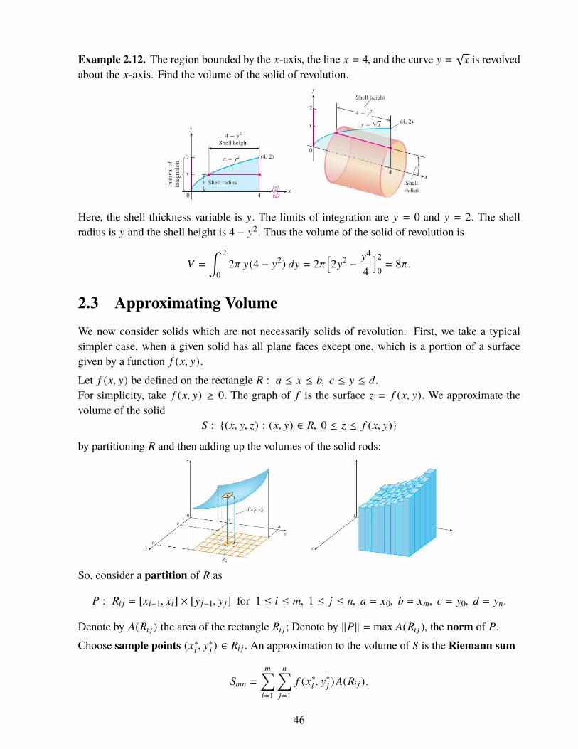
Example 2.12. The region bounded by the x-axis, the line x = 4, and the curve y =√

x is revolvedabout the x-axis. Find the volume of the solid of revolution.

Here, the shell thickness variable is y. The limits of integration are y = 0 and y = 2. The shellradius is y and the shell height is 4 − y2. Thus the volume of the solid of revolution is

V =∫ 2

02π y(4 − y2) dy = 2π

[2y2 −

y4

4]2

0= 8π.

2.3 Approximating VolumeWe now consider solids which are not necessarily solids of revolution. First, we take a typicalsimpler case, when a given solid has all plane faces except one, which is a portion of a surfacegiven by a function f (x, y).

Let f (x, y) be defined on the rectangle R : a ≤ x ≤ b, c ≤ y ≤ d.For simplicity, take f (x, y) ≥ 0. The graph of f is the surface z = f (x, y). We approximate thevolume of the solid

S : {(x, y, z) : (x, y) ∈ R, 0 ≤ z ≤ f (x, y)}

by partitioning R and then adding up the volumes of the solid rods:

So, consider a partition of R as

P : Ri j = [xi−1, xi] × [y j−1, y j] for 1 ≤ i ≤ m, 1 ≤ j ≤ n, a = x0, b = xm, c = y0, d = yn.

Denote by A(Ri j ) the area of the rectangle Ri j ; Denote by ‖P‖ = max A(Ri j ), the norm of P.

Choose sample points (x∗i , y∗j ) ∈ Ri j . An approximation to the volume of S is the Riemann sum

Smn =

m∑i=1

n∑j=1

f (x∗i , y∗j ) A(Ri j ).

46

If limit of Smn exists as ‖P‖ → 0, then this limit is called the double integral of f (x, y). It isdenoted by

!R f (x, y)dA. Whenever the integral exists, it is also enough to consider uniform

partitions, that is, xi − xi−1 = (b − a)/m = ∆x and y j − y j−1 = (d − c)/n = ∆y. In this case, wewrite A(Ri j ) = ∆A = ∆x∆y. Then"

Rf (x, y)dA = lim

‖P‖→0Smn = lim

m→∞limn→∞

m∑i=1

n∑j=1

f (x∗i , y∗j )∆x∆y.

Since f (x, y) ≥ 0, the value of this integral is the volume of the solid S bounded by the rectangleR and the surface z = f (x, y).

When the integral of f (x, y) exists, we say that f is Riemann integrable or just integrable.Riemann sum is well defined even if f is not a positive function. However, the double integralcomputes the signed volume. Analogous to the single variable case, we have the following result;we omit its proof.

Theorem 2.1. Each continuous function defined on a closed bounded rectangle is integrable.

Volumes of solids can also be calculated by using iterated integrals. For example, to find thevolume V of the solid raised over the rectangle R : [0, 2] × [0, 1] and bounded above by the planez = 4 − x − y, we proceed as follows (similar to solids of revolution):

Suppose A(x) is the cross sectional are at x. Then V =∫ 2

0 A(x)dx. Now, A(x) =∫ 1

0 (4− x − y)dy.

Thus, V =∫ 2

0

∫ 10 (4 − x − y)dydx. Therefore,"

R(4 − x − y)dA =

∫ 2

0

∫ 1

0(4 − x − y)dydx.

The expression on the left is a double integral and on the right is an iterated integral.

Theorem 2.2. (Fubini) Let R be the rectangle [a, b] × [c, d]. Let f : R → R be a continuousfunction. Then "

Rf (x, y)dA =

∫ b

a

∫ d

cf (x, y)dydx =

∫ d

c

∫ b

af (x, y)dxdy.

47

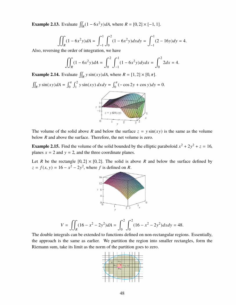
Example 2.13. Evaluate!

R(1 − 6x2y)dA, where R = [0, 2] × [−1, 1].

"R

(1 − 6x2y)dA =∫ 1

−1

∫ 2

0(1 − 6x2y)dxdy =

∫ 1

−1(2 − 16y)dy = 4.

Also, reversing the order of integration, we have"R

(1 − 6x2y)dA =∫ 2

0

∫ 1

−1(1 − 6x2y)dydx =

∫ 2

02dx = 4.

Example 2.14. Evaluate!

R y sin(xy)dA, where R = [1, 2] × [0, π].!R y sin(xy)dA =

∫ π

0

∫ 21 y sin(xy) dxdy =

∫ π

0 (− cos 2y + cos y)dy = 0.

The volume of the solid above R and below the surface z = y sin(xy) is the same as the volumebelow R and above the surface. Therefore, the net volume is zero.

Example 2.15. Find the volume of the solid bounded by the elliptic paraboloid x2 + 2y2 + z = 16,planes x = 2 and y = 2, and the three coordinate planes.

Let R be the rectangle [0, 2] × [0, 2]. The solid is above R and below the surface defined byz = f (x, y) = 16 − x2 − 2y2, where f is defined on R.

V ="

R(16 − x2 − 2y2)dA =

∫ 2

0

∫ 2

0(16 − x2 − 2y2)dxdy = 48.

The double integrals can be extended to functions defined on non-rectangular regions. Essentially,the approach is the same as earlier. We partition the region into smaller rectangles, form theRiemann sum, take its limit as the norm of the partition goes to zero.

48

The double integral of f over such a bounded region R can also be evaluated using iterated integrals.Look at R bounded by two continuous functions g1(x) and g2(x); or, as a region bounded by twocontinuous functions h1(y) and h2(y).

Theorem 2.3. Let f (x, y) be a continuous real valued function on a region R.

1. If R is given by a ≤ x ≤ b, g1(x) ≤ y ≤ g2(x), where g1, g2 : [a, b] → R are continuous,then "

Rf (x, y)dA =

∫ b

a

∫ g2(x)

g1(x)f (x, y)dydx.

2. If R is given by c ≤ y ≤ d, h1(y) ≤ x ≤ h2(y), where h1, h2 : [c, d] → R are continuous,then "

Rf (x, y)dA =

∫ d

c

∫ h2(y)

h1(y)f (x, y)dxdy.

Example 2.16. Find the volume of the prism whose base is the triangle in the xy-plane boundedby the lines y = 0, x = 1 and y = x, and whose top lies in the plane z = 3 − x − y.

V =∫ 1

0

∫ x

0(3 − x − y)dydx =

∫ 1

0(3x − 3x2/2)dx = 1.

Also,

V =∫ 1

0

∫ 1

y

(3 − x − y)dxdy =∫ 1

0(5/2 − 4y + 3y2/2)dy = 1.

Example 2.17. Suppose R is the region bounded by the line x + y = 1 and the portion of the circlex2 + y2 = 1 in the first quadrant. We require to evaluate

!R f (x, y) dA.

49

Sketch it, find the limits, and then write the appropriate integrals. :

"R

f (x, y)dA =∫ 1

0

∫ √1−x2

1−xf (x, y)dydx =

∫ 1

0

∫ √1−y2

1−yf (x, y)dxdy.

For evaluating a double integral as an iterated integral, choose some order: first x, next y. If it doesnot work, or if it is complicated, you may have to choose the reverse order.

Example 2.18. Evaluate!

Rsin x

x dA, where R is the triangle in the xy-plane bounded by the linesy = 0, x = 1, and y = x.

Here, the triangular region R can be expressed as {(x, y) : 0 ≤ y ≤ 1, y ≤ x ≤ 1}.

So, "R

sin xx

dA =∫ 1

0

∫ 1

y

sin xx

dxdy.

We are stuck. No way to proceed further.On the other hand, we express the same R in a different way: {(x, y) : 0 ≤ y ≤ x, 0 ≤ x ≤ 1}. Then

"R

sin xx

dA =∫ 1

0

∫ x

0

sin xx

dydx =∫ 1

0

( sin xx

∫ x

0dy

)dx =

∫ 1

0sin xdx = − cos(1) + 1.

Example 2.19. Evaluate the iterated integral∫ 1

0

∫ 1x sin(y2)dydx.

Write D : 0 ≤ x ≤ 1, x ≤ y ≤ 1.We plan to change the order of integration.

50

∫ 1

0

∫ 1

xsin(y2)dydx =

"D

sin(y2)dA

=

∫ 1

0

∫ y

0sin(y2)dxdy

=

∫ 1

0y sin(y2)dy =

12

(1 − cos(1).

Properties of double integrals with respect to addition, multiplication etc. are as follows.

Theorem 2.4. Let f (x, y) and g(x, y) be continuous on a region D. Let c be a constant.

1. (Constant Multiple):!

D c f (x, y)dA = c!

D f (x, y)dA.

2. (Sum-Difference):!

D[ f (x, y) ± g(x, y)]dA =!

D f (x, y)dA ±!

D g(x, y)dA.

3. (Additivity):!

D∪R f (x, y)dA =!

D f (x, y)dA +!

R f (x, y)dA,provided f (x, y) is continuous on a region R also, and D and R are non-overlapping.

4. (Domination): If f (x, y) ≤ g(x, y) in D, then!

D f (x, y)dA ≤!

D g(x, y)dA.

5. (Area):!

D 1 dA = ∆(D) = Area of D.

6. (Boundedness): If m ≤ f (x, y) ≤ M in D, then m∆(D) ≤!

D f (x, y)dA ≤ M∆(D).

2.4 Riemann Sum in Polar coordinatesSuppose R is one of the following regions in the plane:

It is easy to describe such regions in polar coordinates. Using polar coordinates, we define a polarrectangle as a region given in the form:

R = {(r, θ) : a ≤ r ≤ b, α ≤ θ ≤ β, β − α ≤ 2π}.

We can divide a polar rectangle into polar subrectangles as in the following:

51

Ri j = {(r, θ) : ri−1 ≤ r ≤ ri, θ j−1 ≤ θ ≤ θ j }.

Suppose f is a real valued function defined on a polar rectangle R. Let P be a partition of R intosmaller polar rectangles Ri j . The area of Ri j is

∆(Ri j ) =12

(r2i − r2

i−1)(θ j − θ j−1).

Take a uniform grid dividing r into m equal parts and θ into n equal parts. Write ri − ri−1 = ∆rand θ j − θ j−1 = ∆θ. Also write the mid-point of ri−1 and ri as r∗i =

12 (ri + ri−1), similarly,

θ∗j =12 (θ j−1 + θ j ). Then the Riemann sum for f (r, θ) can be written as

S =m∑

i=1

n∑j=1

f (r∗i , θ∗j )∆(Ri j ) =

m∑i=1

n∑j=1

f (r∗i , θ∗j )r∗i ∆r∆θ.

Therefore, if f (r, θ) is continuous on the polar rectangle R, then"R

f (r, θ)dA ="

Rf (r, θ) r dr dθ

If f (x, y), in Cartesian coordinates, is continuous on the polar rectangle R, then converting thisinto polar form, we have"

Rf (x, y)dA =

∫ β

α

∫ b

af (r cos θ, r sin θ) r dr dθ.

The double integral in polar form can be generalized to functions defined on regions other thanpolar rectangles. Let f be a continuous function defined over a region bounded by the raysθ = α, θ = β and the continuous curves r = g1(θ), r = g2(θ).

Then "R

f (r, θ)dA =∫ β

α

∫ g2(θ)

g1(θ)f (r, θ) r dr dθ.

Caution: Do not forget the r on the right hand side.

Example 2.20. Find the limits of integration for integrating f (r, θ) over the region R that liesinside the cardioid r = 1 + cos θ and outside the circle x2 + y2 = 1.

52

Better write the circle as r = 1. Now, R is the region:

"R

f (r, θ)dA =∫ π/2

−π/2

∫ 1+cos θ

1f (r, θ)r dr dθ.

Example 2.21. Evaluate I =∫ 1

0

∫ √1−x2

0 (x2 + y2)dydx.

The limits of integration say that the region is the quarter of the unit disk in the first quadrant:

The region in polar coordinates is R : 0 ≤ r ≤ 1, 0 ≤ θ ≤ π/2.Changing to polar coordinates, we have x = r cos θ, y = r sin θ and then

I =∫ 1

0

∫ π/2

0r2 r dr dθ =

∫ π/2

0

14

dθ =π

8.

Example 2.22. Evaluate I =∫ 1−1

∫ √1−x2

0 ex2+y2dydx.

The region is the upper semi-unit-disk, whose polar description is

R = {(r, θ) : 0 ≤ r ≤ 1, 0 ≤ θ ≤ π}.

Then I =!

R ex2+y2dA. Using integration in polar form,

I =∫ π

0

∫ 1

0er2

r dr dθ =∫ π

0

[ 12

er2 ]1

0dθ =

∫ π

0

e − 12

dθ =π

2(e − 1).

Example 2.23. Evaluate!

R(3x + 4y2)dA, where R is the region in the upper half plane boundedby the circles x2 + y2 = 1 and x2 + y2 = 4.

53

R = {(r, θ) : 1 ≤ r ≤ 2, 0 ≤ θ ≤ π}. Therefore,"R

(3x + 4y2)dA =∫ π

0

∫ 2

1(3r cos θ + 4r2 sin2 θ)r dr dθ

=

∫ π

0

[r3 cos θ + r4 sin2 θ

]2

1dθ =

∫ π

0(7 cos θ + 15 sin2 θ) dθ =

15π2.

Example 2.24. Find the area enclosed by one of the four leaves of the curve r = cos(2θ).

The region is R = {(r, θ) : −π/4 ≤ θ ≤ π/4, 0 ≤ r ≤ cos(2θ)}.

Then the required area is"R

dA =∫ π/4

−π/4

∫ cos(2θ)

0r dr dθ =

∫ π/4

−π/4

cos2(2θ) − 12

dθ =∫ π/4

−π/4

cos(4θ) − 14

dθ =π

8.

Example 2.25. Find the volume of the solid that lies under the paraboloid z = x2 + y2, above thexy-plane, and inside the cylinder x2 + y2 = 2x.

The solid lies above the disk D whose boundary has equation x2 + y2 = 2x, or in polar coordinates,r2 = 2r cos θ, or r = 2 cos θ.

The disk D = {(r, θ) : −π/2 ≤ θ ≤ π/2, 0 ≤ r ≤ 2 cos θ}.Then the required volume V is given by

V ="

D

(x2+y2)dA =∫ π/2

−π/2

∫ 2 cos θ

0r2 r dr dθ =

∫ π/2

−π/24 cos4 θ dθ =

∫ π/2

−π/2(3+cos 4θ+4 cos 2θ) dθ =

3π2.

54

2.5 Triple IntegralLet f (x, y, z) be a real valued function defined on a bounded region D in R3. As earlier we dividethe region into smaller cubes enclosed by planes parallel to the coordinate planes. The set of thesesmaller cubes is called a partition P. The norm of the partition is the maximum volume enclosedby any smaller cube. Then form the Riemann sum S and take its limit as the cubes become smallerand smaller. If the limit exists, we say that the limit is the triple integral of the function over theregion D.$

Df (x, y, z)dV = lim

‖P‖→0

∑f (x∗i , y

∗j , z∗k )(xi − xi−1)(y j − y j−1)(zk − zk−1),

where (x∗i , y∗j , z∗k ) is a point in the (i, j, k)-th cube in the partition.

As earlier, Fubuni’s theorem says that for continuous functions, if the region D can be written as

D = {(x, y, z) : a ≤ x ≤ b, g1(x) ≤ y ≤ g2(x), h1(x, y) ≤ z ≤ h2(x, y)},

then the triple integral can be written as an iterated integral:$D

f (x, y, z)dV =∫ b

a

∫ g2(x)

g1(x)

∫ h2(x,y)

h1(x,y)f (x, y, z)dz dy dx.

To find the limits of integration, we first sketch the region D along with its shadow on the xy-plane.Next, we find the z-limits, then y-limits and then x-limits.

Observe that the volume of D is#

D 1 dV .

All properties for double integrals hold analogously for triple integrals.

Example 2.26. Find the volume of the solid enclosed by the surfaces z = x2 + 3y2 andz = 8 − x2 − y2.

55

Eliminating z from the two equations, we get the projection of the solid on the xy-plane, whichis x2 + 2y2 = 4. This gives the limits of integration for y as ±

√(4 − x2)/2. Clearly, −2 ≤ x ≤ 2.

Therefore,

V =

$D

dV =∫ 2

−2

∫ √(4−x2)/2

−√

(4−x2)/2

∫ 8−x2−y2

x2+3y2dz dy dx

=

∫ 2

−2

∫ √(4−x2)/2

−√

(4−x2)/2(8 − 2x2 − 4y2) dy dx

=

∫ 2

−2

[(8 − 2x2)y −

43y3

] y=√

(4−x2)/2

y=−√

(4−x2)/2dx

=

∫ 2

−2

[8(4 − x2

2)3/2−

83(4 − x2

2)3/2

]dx

=4√

23

∫ 2

−2(4 − x2)3/2 dx = 8π

√2.

Notice that changing the order of integration involves expressing the region by choosing differentorder of the limits of values in the axes.

Example 2.27. Write the integral of f (x, y, z) over a tetrahedron with vertices at (0, 0, 0), (1, 1, 0),(0, 1, 0), and (0, 1, 1) as an iterated integral.

First, sketch the region D to see the limits geometrically. The right hand side bounding surface ofD lies in the plane y = 1. The left hand side bounding surface lies in the plane y = z + x. Theprojection of D on the zx-plane is R. The upper boundary of R is the line z = 1 − x. The lowerboundary of R is the line z = 0.To find the y-limits for D, we consider a typical point (x, z) in R and a line through this pointparallel to y-axis. It enters D at y = x + z and leaves at y = 1.To find the z-limits for D, we find that the line L through (x, z) parallel to z-axis enters R at z = 0and leaves R at z = 1 − x.

56

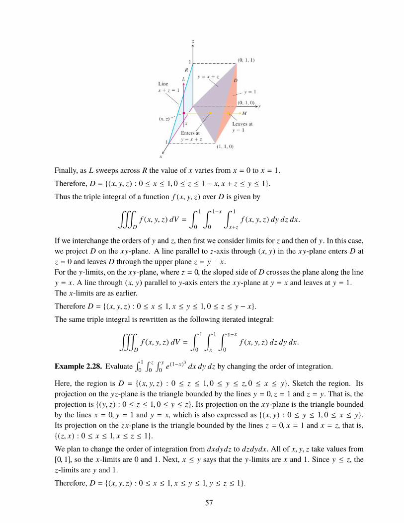
Finally, as L sweeps across R the value of x varies from x = 0 to x = 1.Therefore, D = {(x, y, z) : 0 ≤ x ≤ 1, 0 ≤ z ≤ 1 − x, x + z ≤ y ≤ 1}.Thus the triple integral of a function f (x, y, z) over D is given by$

Df (x, y, z) dV =

∫ 1

0

∫ 1−x

0

∫ 1

x+zf (x, y, z) dy dz dx.

If we interchange the orders of y and z, then first we consider limits for z and then of y. In this case,we project D on the xy-plane. A line parallel to z-axis through (x, y) in the xy-plane enters D atz = 0 and leaves D through the upper plane z = y − x.For the y-limits, on the xy-plane, where z = 0, the sloped side of D crosses the plane along the liney = x. A line through (x, y) parallel to y-axis enters the xy-plane at y = x and leaves at y = 1.The x-limits are as earlier.Therefore D = {(x, y, z) : 0 ≤ x ≤ 1, x ≤ y ≤ 1, 0 ≤ z ≤ y − x}.

The same triple integral is rewritten as the following iterated integral:$D

f (x, y, z) dV =∫ 1

0

∫ 1

x

∫ y−x

0f (x, y, z) dz dy dx.

Example 2.28. Evaluate∫ 1

0

∫ z0

∫ y

0 e(1−x)3dx dy dz by changing the order of integration.

Here, the region is D = {(x, y, z) : 0 ≤ z ≤ 1, 0 ≤ y ≤ z, 0 ≤ x ≤ y}. Sketch the region. Itsprojection on the yz-plane is the triangle bounded by the lines y = 0, z = 1 and z = y. That is, theprojection is {(y, z) : 0 ≤ z ≤ 1, 0 ≤ y ≤ z}. Its projection on the xy-plane is the triangle boundedby the lines x = 0, y = 1 and y = x, which is also expressed as {(x, y) : 0 ≤ y ≤ 1, 0 ≤ x ≤ y}.

Its projection on the zx-plane is the triangle bounded by the lines z = 0, x = 1 and x = z, that is,{(z, x) : 0 ≤ x ≤ 1, x ≤ z ≤ 1}.We plan to change the order of integration from dxdydz to dzdydx. All of x, y, z take values from[0, 1], so the x-limits are 0 and 1. Next, x ≤ y says that the y-limits are x and 1. Since y ≤ z, thez-limits are y and 1.Therefore, D = {(x, y, z) : 0 ≤ x ≤ 1, x ≤ y ≤ 1, y ≤ z ≤ 1}.

57

∫ 1

0

∫ z

0

∫ y

0e(1−x)3

dx dy dz =∫ 1

0

∫ 1

x

∫ 1

y

e(1−x)3dz dy dx

=

∫ 1

0

∫ 1

x(1 − y)e(1−x)3

dy dx =∫ 1

0

(1 − x)2

2e(1−x)3

dx

= −

∫ 0

(1−0)3

et

6dt =

e − 16

. with t = (1 − x)3

2.6 Triple Integral in Cylindrical coordinatesCylindrical coordinates express a point P in space as a triple (r, θ, z), where (r, θ) is the polarrepresentation of the projection of P on the xy-plane.

If P has Cartesian representation (x, y, z) and cylindrical representation (r, θ, z), then

x = r cos θ, y = r sin θ, z = z, r2 = x2 + y2, tan θ = y/x.

In cylindrical coordinates,r = a describes a cylinder with axis as z-axis.θ = α describes a plane containing the z-axis.z = b describes a plane perpendicular to z-axis.

The Riemann sum of f (r, θ, z) uses a partition of D into cylindrical wedges:

The volume element dV = r dr dθdz. Thus the triple integral is$D

f (r, θ, z)dV =$

Df (r, θ, z)r dr dθ dz.

Its conversion to iterated integrals uses a similar technique of determining the limits of integration.

Example 2.29. Find the limits of integration in cylindrical coordinates for integrating a functionf (r, θ, z) over the region D bounded below by the plane z = 0, laterally by the circular cylinderx2 + (y − 1)2 = 1, and above by the paraboloid z = x2 + y2.

58

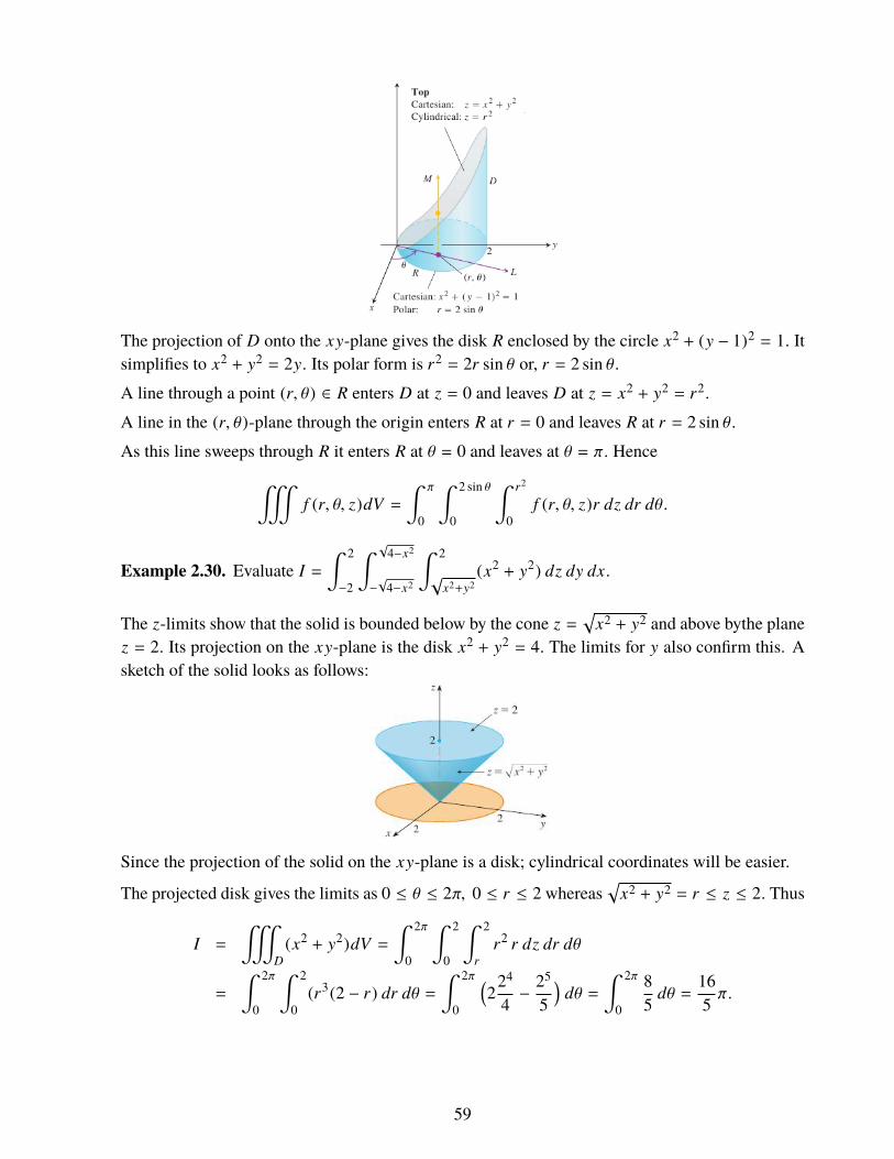
The projection of D onto the xy-plane gives the disk R enclosed by the circle x2 + (y − 1)2 = 1. Itsimplifies to x2 + y2 = 2y. Its polar form is r2 = 2r sin θ or, r = 2 sin θ.A line through a point (r, θ) ∈ R enters D at z = 0 and leaves D at z = x2 + y2 = r2.

A line in the (r, θ)-plane through the origin enters R at r = 0 and leaves R at r = 2 sin θ.As this line sweeps through R it enters R at θ = 0 and leaves at θ = π. Hence$

f (r, θ, z)dV =∫ π

0

∫ 2 sin θ

0

∫ r2

0f (r, θ, z)r dz dr dθ.

Example 2.30. Evaluate I =∫ 2

−2

∫ √4−x2

−√

4−x2

∫ 2

√x2+y2

(x2 + y2) dz dy dx.

The z-limits show that the solid is bounded below by the cone z =√

x2 + y2 and above bythe planez = 2. Its projection on the xy-plane is the disk x2 + y2 = 4. The limits for y also confirm this. Asketch of the solid looks as follows:

Since the projection of the solid on the xy-plane is a disk; cylindrical coordinates will be easier.

The projected disk gives the limits as 0 ≤ θ ≤ 2π, 0 ≤ r ≤ 2 whereas√

x2 + y2 = r ≤ z ≤ 2. Thus

I =$

D(x2 + y2)dV =

∫ 2π

0

∫ 2

0

∫ 2

rr2 r dz dr dθ

=

∫ 2π

0

∫ 2

0(r3(2 − r) dr dθ =

∫ 2π

0

(2

24

4−

25

5)

dθ =∫ 2π

0

85

dθ =165π.

59

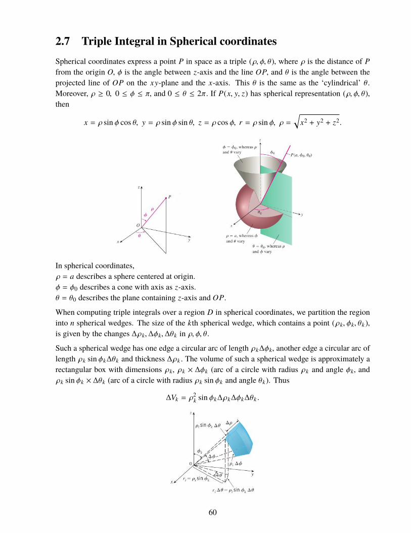
2.7 Triple Integral in Spherical coordinatesSpherical coordinates express a point P in space as a triple (ρ, φ, θ), where ρ is the distance of Pfrom the origin O, φ is the angle between z-axis and the line OP, and θ is the angle between theprojected line of OP on the xy-plane and the x-axis. This θ is the same as the ‘cylindrical’ θ.Moreover, ρ ≥ 0, 0 ≤ φ ≤ π, and 0 ≤ θ ≤ 2π. If P(x, y, z) has spherical representation (ρ, φ, θ),then

x = ρ sin φ cos θ, y = ρ sin φ sin θ, z = ρ cos φ, r = ρ sin φ, ρ =√

x2 + y2 + z2.

In spherical coordinates,ρ = a describes a sphere centered at origin.φ = φ0 describes a cone with axis as z-axis.θ = θ0 describes the plane containing z-axis and OP.

When computing triple integrals over a region D in spherical coordinates, we partition the regioninto n spherical wedges. The size of the kth spherical wedge, which contains a point (ρk, φk, θk ),is given by the changes ∆ρk,∆φk,∆θk in ρ, φ, θ.

Such a spherical wedge has one edge a circular arc of length ρk∆φk, another edge a circular arc oflength ρk sin φk∆θk and thickness ∆ρk . The volume of such a spherical wedge is approximately arectangular box with dimensions ρk, ρk × ∆φk (arc of a circle with radius ρk and angle φk, andρk sin φk × ∆θk (arc of a circle with radius ρk sin φk and angle θk). Thus

∆Vk = ρ2k sin φk∆ρk∆φk∆θk .

60

The corresponding Riemann sum is S =∑n

k=1 f (ρk, φk, θk )ρ2k sin φk∆ρk∆φk∆θk . Accordingly,$

Df (ρ, φ, θ)dV =

$D

f (ρ, φ, θ)ρ2 sin φ dρ dφ dθ.

The procedure in computing a triple integral in spherical coordinates is similar to that in cylindricalcoordinates:Sketch the region D and its projection on the xy-plane. Then find the ρ limit, φ limit and θ limit.

$D

f (ρ, φ, θ)dV =∫ β

α

∫ φ−max

φ−min

∫ g2(φ,θ)

g1(φ,θf (ρ, φ, θ)ρ2 sin φ dρ dφ dθ.

Example 2.31. Find the volume of the solid D cut from the ball ρ ≤ 1 by the cone φ = π/3.

Draw a ray M through D from the origin making an angle φwith the z-axis. Draw also its projectionL on the xy-plane. The line L makes an angle θ with the x-axis. Let R be the projected region ofD in the xy-plane.

M enters D at ρ = 0 and leaves D at ρ = 1.Angle φ runs through 0 to π/3, since D is bounded by the cone φ = π/3.L sweeps through R as θ varies from 0 to 2π. Thus

V =

$Dρ2 sin φ dV =

∫ 2π

0

∫ π/3

0

∫ 1

0ρ2 sin φ dρ dφ dθ

=

∫ 2π

0

∫ π/3

0

13

sin φ dφ dθ =∫ 2π

0

[− cos φ3

]π/30=

16

2π =π

3.

61

Example 2.32. Evaluate I =∫ 1

−1

∫ √1−x2

−√

1−x2

∫ √1−x2−y2

−√

1−x2−y2e(x2+y2+z2)3/2

dz dy dx.

Notice that I =#

D e(x2+y2+z2)3/2dV, where D is the unit ball.

Writing in spherical coordinates, I =#

D eρ3dV . Then converting to iterated integral,

I =∫ 1

0

∫ π

0

∫ 2π

0eρ

3ρ2 sin φ dρ dφ dθ.

Since the integrand is a product of separate functions of ρ, of φ, of θ,

I =∫ 1

0eρ

3ρ2 dρ

∫ π

0sin φ dφ

∫ 2π

0dθ =

[ eρ3

3]1

0

[− cos φ

]π0

(2π) =4π3

(e − 1).

2.8 Change of VariablesThe change of coordinate system from Cartesian to Cylindrical or to Spherical are examples ofchange of variables. Let us consider what happens when a different type of change of variablesoccurs.Suppose f maps a region D in R2 onto a region R in R2 in a one-one manner. For convenience,we say that D is a region in the uv-plane and R is a region in the xy-plane; and f maps (u, v) to(x, y). Then f can be thought of as a pair of maps: ( f1, f2). That is, x = f1(u, v) and y = f2(u, v).We often show this dependence implicitly by writing

x = x(u, v), y = y(u, v).

Example 2.33. What is the image of D = {(u, v) : 0 ≤ u ≤ 1, 0 ≤ v ≤ 1} under the the map givenby x = u2 − v2, y = 2uv ?

Let us see the boundaries of the square D : 0 ≤ u ≤ 1, 0 ≤ v ≤ 1.The lower boundary is the line segment 0 ≤ u ≤ 1, v = 0. It is transformed to the line segmentx = u2, y = 0 or in the xy-plane it is the line segment 0 ≤ x ≤ 1, y = 0.The left boundary of D is the line segment u = 0, 0 ≤ v ≤ 1. It is transformed to x = −v2, y = 0.This is the line segment joining (0, 0) to (−1, 0) in the xy-plane.The upper boundary line of D is the line segment 0 ≤ u ≤ 1, v = 1. This is transformed tox = u2 − 1, y = 2u. Eliminating u from these equations, we get the arc of the curve x = y2

4 − 1joining the points (−1, 0) to (0, 2) in the xy-plane.The right hand side boundary of D is the line segment u = 1 and v varying from 1 to 0. This istransformed to x = 1− v2, y = 2v. Eliminating v from these equations we have the arc of the curvex = 1 − y2

4 joining the points (0, 2) to (1, 0).

The interior of D is mapped onto the interior of the so obtained region R in the xy-plane whoseboundary are the line segments and the arcs. This transformation is shown is the picture below.

62

If (u, v) 7→ (x, y), then how does area of a small rectangle change?A typical small rectangle with sides ∆u and ∆v has corners at the points

A1 = (a, b), A2 = (a + ∆u, b), A3 = (a, b + ∆v), A4 = (a + ∆u, b + ∆v).

Let the images of Ak under (u, v) 7→ (x, y) be Bk = (ak, bk ) for k = 1, 2, 3, 4. Thena1 = x(a, b)a2 = x(a + ∆u, b) ≈ x(a, b) + xu∆ua3 = x(a, b + ∆v) ≈ x(a, b) + xv∆va4 = x(a + ∆u, b + ∆v) ≈ x(a, b) + xu∆u + xv∆v

Here, xu = xu(a, b) and xv = xv (a, b). Similar approximations hold for b1, b2, b3, b4.

Now, Area of the image of the rectangle A1 A2 A3 A4 is approximately equal to the area of theparallelogram B1B2B3B4 in xy-plane, which is twice the area of the triangle B1B2B4 and is

|(a4 − a1)(b4 − b2) − (a4 − a2)(b4 − b1) | =�����det

[xu xvyu yv

] �����(a, b)∆u∆v.

This determinant is called theJacobianof themap (u, v) 7→ (x, y); and is denoted by J (x(u, v), y(u, v)).

The Jacobian is also written as J = J (x(u, v), y(u, v)) =∂(x, y)∂(u, v)

.

We write this as Area of image of a rectangle with one corner at (a, b) and sides of length ∆u and∆v is approximately |J (x(u, v), y(u, v) |∆u∆v, where the Jacobian J (·, ·) is evaluated at (a, b).

In deriving this approximation, we have assumed that xu, xv, yu, yv are continuous.Assume that x = x(u, v) and y = y(u, v) have continuous partial derivatives with respect to u andv. Assume also that a region D in the uv-plane is in one-one correspondence with a region R inthe xy-plane by the map (u, v) 7→ (x, y). Let f (x, y) be a real valued continuous function on theregion R. Then we have the map f (u, v) = f (x(u, v), y(u, v)).

To see how the integrals of f over R and integral of f over D are related, divide D in the uv-planeinto smaller rectangles. Now, the images of the smaller rectangles are related by

Area of R = |J |Area of D = ���∂(x, y)∂(u, v)

��� Area of D.

By forming the Riemann sum and taking the limit, we obtain:"R

f (x, y)dA ="

Df (u, v) |J (x(u, v), y(u, v) | dA =

"D

f (u, v) ���∂(x, y)∂(u, v)

��� dA.

63

For example, in the case of polar coordinates, we have

x = x(r, θ) = r cos θ, y = y(r, θ) = r sin θ.

Thus, the Jacobian is

J (x(r, θ), y(r, θ)) = xr yθ − xθ yr = cos θ(r cos θ) − (−r sin θ) sin θ = r .

Therefore, the double integral in polar coordinates for a function f (x, y) takes the form"R

f (x, y)dA ="

Df (r cos θ, r sin θ) r dA.

as we had seen earlier.For x = x(u, v,w), y = y(u, v,w), z = z(u, v,w), we write the Jacobian as

J = J (x(u, v,w), y(u, v,w), z(u, v,w)) =∂(x, y, z)∂(u, v,w)

= det

xu xv xwyu yv ywzu zv zw

.

If R is the region in R3 on which f has been defined and D is the region in the uvw-space so thatthe functions x, y, z map D onto R in a one-one manner, then$

Rf (x, y, z)dV =

$D

f (x(u, v,w), y(u, v,w), z(u, v,w))�����∂(x, y, z)∂(u, v,w)

�����du dv dw.

In the case of cylindrical coordinates, x = r cos θ, y = r sin θ, z = z. The absolute value of theJacobian is

�����∂(x, y, z)∂(r, θ, z)

�����=

��������det

xr xθ xz

yr yθ yz

zr zθ zz

��������= r .

$R

f (x, y, z)dV =$

Df (r cos θ, r sin θ, z) r dr dθ dz.

For the spherical coordinates, we see that

x = ρ sin φ cos θ, y = ρ sin φ sin θ, z = ρ cos φ.

The triple integral looks like$R

f (x, y, z)dV =$

Df (ρ sin φ cos θ, ρ sin φ sin θ, ρ cos φ)ρ2 sin φ dρ dφ dθ.

We had already derived these results independently.These formulas help us in evaluating double and triple integrals in x, y, z as integrals in u, v,w bychoosing a transformation (u, v,w) 7→ (x, y, z) suitably.

Example 2.34. Evaluate the double integral!

R(y − x)dA, where R is the region bounded by thelines y − x = 1, y − x = −3, 3y + x = 7, 3y + x = 15.

64

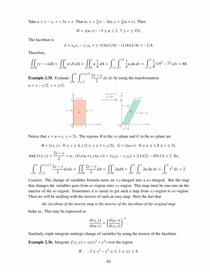
Take u = y − x, v = 3y + x. That is, x = 14 (v − 3u), y = 1

4 (u + v). Then

D = {(u, v) : −3 ≤ u ≤ 1, 7 ≤ v ≤ 15}.

The Jacobian isJ = xuyv − xvyu = (−3/4)(1/4) − (1/4)(1/4) = −1/4.

Therefore,"R

(y − x)dA ="

Du |J | dA =

"D

u14

dA =∫ 1

−3

∫ 15

7

14

u du dv =∫ 1

−3

18

(152 − 72) dv = 88.

Example 2.35. Evaluate∫ 4

0

∫ 1+y/2

y/2

2x − y

2dx dy by using the transformation

u = x − y/2, v = y/2.

Notice that x = u + v, y = 2v. The regions R in the xy-plane and G in the uv-plane are

R = {(x, y) : 0 ≤ y ≤ 4, y/2 ≤ x ≤ 1 + y/2}, G = {(u, v) : 0 ≤ u ≤ 1, 0 ≤ v ≤ 2}.

And f (x, y) =2x − y

2= u, |J (x(u, v), y(u, v) | = |xuyv − xvyu | = |(1)(2) − (0)(1) | = 2. So,

∫ 4

0

∫ 1+y/2

y/2

2x − y

2dxdy =

"R

2x − y

2dA =

"G

2udA =∫ 2

0

∫ 1

02u du dv =

∫ 2

012 dv = 2.

Caution: The change of variables formula turns an xy-integral into a uv-integral. But the mapthat changes the variables goes from uv-region onto xy-region. This map must be one-one on theinterior of the uv-region. Sometimes it is easier to get such a map from xy-region to uv-region.Then we will be tackling with the inverse of such an easy map. Here the fact that

the Jacobian of the inverse map is the inverse of the Jacobian of the original map

helps us. This may be expressed as

∂(x, y)∂(u, v)

=

(∂(u, v)∂(x, y)

)−1.

Similarly, triple integrals undergo change of variables by using the inverse of the Jacobian.

Example 2.36. Integrate f (x, y) = xy(x2 + y2) over the region

R : −3 ≤ x2 − y2 ≤ 3, 1 ≤ xy ≤ 4.

65

There is a simple map that goes in the wrong direction: u = x2 − y2, v = xy. Then the image of R,which we denote as D in the uv-plane is the rectangle

D : −3 ≤ u ≤ 3, 1 ≤ v ≤ 4.

We have F : D → R defined by F (x, y) = (u, v) = (x2 − y2, xy). And its inverse is G = F−1, whereG : R→ D.

We need not compute the map G. Instead, we go for the Jacobian.

∂(u, v)∂(x, y)

= det[ux uy

vx vy

]= det

[2x −2yy x

]= 2(x2 + y2).

Therefore,∂(x, y)∂(u, v)

=1

2(x2 + y2). Then

"R

xy(x2 + y2) dA ="

D

[xy(x2 + y2)

�����1

2(x2 + y2)

�����

]dA.

Notice that the integral on the right side is in the uv-plane and the bracketed term inside [ · ] is afunction of (u, v). Since the bracketed term simplifies to xy/2 which is equal to v/2, we have theintegral as"

D

v

2dA =

12

∫ 3

−3

∫ 4

1v dv du =

12

∫ 3

−3

42 − 12

2du =

154

[3 − (−3)

]=

452.

2.9 Review ProblemsProblem 1: Find the area of the region bounded by the curves y = x and y = 2 − x2.

The points of intersection of the curves satisfy y = x and x = 2 − x2. The last equation is same as(x + 2)(x − 1) = 0. Thus the points of intersection are (−2,−2) and (1, 1). Hence the area is

���

∫ 1

−2

∫ 2−x2

xdydx��� =

���

∫ 1

−2(2 − x2 − x)dx��� =

���[2x −

x3

3−

x2

2]1

−2��� =

92.

Since the significant portion of the curve y = 2 − x2 lies above the portion of the line y = x, thereis no need to take the absolute value. The calculation also confirms this.

Problem 2: Evaluate I =!

D (4 − x2 − y2) dA if D is the region bounded by the straight linesx = 0, x = 1, y = 0 and y = 3/2.

66

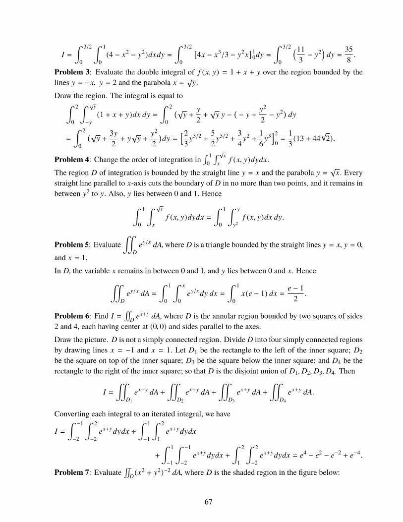
I =∫ 3/2

0

∫ 1

0(4 − x2 − y2)dxdy =

∫ 3/2

0

[4x − x3/3 − y2x

]10dy =

∫ 3/2

0

(113− y2

)dy =

358.

Problem 3: Evaluate the double integral of f (x, y) = 1 + x + y over the region bounded by thelines y = −x, y = 2 and the parabola x =

√y.

Draw the region. The integral is equal to∫ 2

0

∫ √y

−y

(1 + x + y)dx dy =∫ 2

0

(√y +

y

2+√y y −

(− y +

y2

2− y2) dy

=

∫ 2

0

(√y +

3y2+ y√y +

y2

2)dy =

[23y3/2 +

52y5/2 +

34y2 +

16y3

]2

0=

13

(13 + 44√

2).

Problem 4: Change the order of integration in∫ 1

0

∫ √xx f (x, y)dydx.

The region D of integration is bounded by the straight line y = x and the parabola y =√

x. Everystraight line parallel to x-axis cuts the boundary of D in no more than two points, and it remains inbetween y2 to y. Also, y lies between 0 and 1. Hence∫ 1

0

∫ √x

xf (x, y)dydx =

∫ 1

0

∫ y

y2f (x, y)dx dy.

Problem 5: Evaluate"

Dey/x dA,where D is a triangle bounded by the straight lines y = x, y = 0,

and x = 1.In D, the variable x remains in between 0 and 1, and y lies between 0 and x. Hence"

Dey/x dA =

∫ 1

0

∫ x

0ey/xdy dx =

∫ 1

0x(e − 1) dx =

e − 12

.

Problem 6: Find I =!

D ex+y dA, where D is the annular region bounded by two squares of sides2 and 4, each having center at (0, 0) and sides parallel to the axes.Draw the picture. D is not a simply connected region. Divide D into four simply connected regionsby drawing lines x = −1 and x = 1. Let D1 be the rectangle to the left of the inner square; D2be the square on top of the inner square; D3 be the square below the inner square; and D4 be therectangle to the right of the inner square; so that D is the disjoint union of D1, D2, D3, D4. Then

I ="

D1

ex+y dA +"

D2

ex+y dA +"

D3

ex+y dA +"

D4

ex+y dA.

Converting each integral to an iterated integral, we have

I =∫ −1

−2

∫ 2

−2ex+ydydx +

∫ 1

−1

∫ 2

1ex+ydydx

+

∫ 1

−1

∫ −1

−2ex+ydydx +

∫ 2

1

∫ 2

−2ex+ydydx = e4 − e2 − e−2 + e−4.

Problem 7: Evaluate!

D (x2 + y2)−2 dA, where D is the shaded region in the figure below:

67

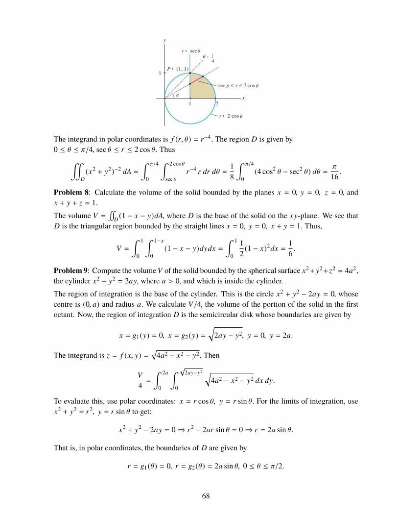
The integrand in polar coordinates is f (r, θ) = r−4. The region D is given by0 ≤ θ ≤ π/4, sec θ ≤ r ≤ 2 cos θ. Thus"

D(x2 + y2)−2 dA =

∫ π/4

0

∫ 2 cos θ

sec θr−4 r dr dθ =

18

∫ π/4

0(4 cos2 θ − sec2 θ) dθ =

π

16.

Problem 8: Calculate the volume of the solid bounded by the planes x = 0, y = 0, z = 0, andx + y + z = 1.The volume V =

!D (1 − x − y)dA, where D is the base of the solid on the xy-plane. We see that

D is the triangular region bounded by the straight lines x = 0, y = 0, x + y = 1. Thus,

V =∫ 1

0

∫ 1−x

0(1 − x − y)dydx =

∫ 1

0

12

(1 − x)2dx =16.

Problem 9: Compute the volumeV of the solid bounded by the spherical surface x2+y2+ z2 = 4a2,the cylinder x2 + y2 = 2ay, where a > 0, and which is inside the cylinder.The region of integration is the base of the cylinder. This is the circle x2 + y2 − 2ay = 0, whosecentre is (0, a) and radius a. We calculate V/4, the volume of the portion of the solid in the firstoctant. Now, the region of integration D is the semicircular disk whose boundaries are given by

x = g1(y) = 0, x = g2(y) =√

2ay − y2, y = 0, y = 2a.

The integrand is z = f (x, y) =√

4a2 − x2 − y2. Then

V4=

∫ 2a

0

∫ √2ay−y2

0

√4a2 − x2 − y2 dx dy.

To evaluate this, use polar coordinates: x = r cos θ, y = r sin θ. For the limits of integration, usex2 + y2 = r2, y = r sin θ to get:

x2 + y2 − 2ay = 0⇒ r2 − 2ar sin θ = 0⇒ r = 2a sin θ.

That is, in polar coordinates, the boundaries of D are given by

r = g1(θ) = 0, r = g2(θ) = 2a sin θ, 0 ≤ θ ≤ π/2.

68

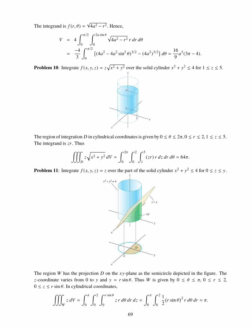
The integrand is f (r, θ) =√

4a2 − r2. Hence,

V = 4∫ π/2

0

∫ 2a sin θ

0

√4a2 − r2 r dr dθ

=−43

∫ π/2

0

[(4a2 − 4a2 sin2 θ)3/2 − (4a2)3/2] dθ =

169

a3(3π − 4).

Problem 10: Integrate f (x, y, z) = z√

x2 + y2 over the solid cylinder x2 + y2 ≤ 4 for 1 ≤ z ≤ 5.

The region of integration D in cylindrical coordinates is given by 0 ≤ θ ≤ 2π, 0 ≤ r ≤ 2, 1 ≤ z ≤ 5.The integrand is zr . Thus$

Dz√

x2 + y2 dV =∫ 2π

0

∫ 2

0

∫ 5

1(zr) r dz dr dθ = 64π.

Problem 11: Integrate f (x, y, z) = z over the part of the solid cylinder x2 + y2 ≤ 4 for 0 ≤ z ≤ y.

The region W has the projection D on the xy-plane as the semicircle depicted in the figure. Thez-coordinate varies from 0 to y and y = r sin θ. Thus W is given by 0 ≤ θ ≤ π, 0 ≤ r ≤ 2,0 ≤ z ≤ r sin θ. In cylindrical coordinates,$

Wz dV =

∫ π

0

∫ 2

0

∫ r sin θ

0z r dθ dr dz =

∫ π

0

∫ 2

0

12(r sin θ

)2 r dθ dr = π.

69

Problem 12: Compute#

D z dV, where D is the solid lying above the cone x2+ y2 = z2 and belowthe unit sphere.

The upper branch of the cone, which is relevant to D, has the equation φ = π/4 in sphericalcoordinates. The sphere has the equation ρ = 1. Thus D is given by

D : 0 ≤ θ ≤ 2π, 0 ≤ φ ≤ π/4, 0 ≤ ρ ≤ 1.

Since z = ρ cos φ, the required integral is$D

z dV =

∫ 2π

0

∫ π/4

0

∫ 1

0(ρ cos φ)ρ2 sin φ dρ dφ dθ

= 2π∫ π/4

0

∫ 1

0ρ3 cos φ sin φ dρ dφ =

π

2

∫ π/4

0cos φ sin φ dφ =

π

8.

Problem 13: Evaluate I =∫ ∞−∞

e−x2dx.

I2 = lima→∞

( ∫ a

−ae−x2

dx)2= lim

a→∞

[( ∫ a

−ae−x2

dx) ( ∫ a

−ae−y

2dy

)]

= lima→∞

[ ∫ a

−a

∫ a

−ae−x2−y2

dx dy]= lim

a→∞

"R

e−x2−y2dA

where R is the square [−a, a] × [−a, a] for a > 0.Let D = B(0, a) and S = B(0,

√2 a), the balls centred at 0 and with radii a and

√2 a, respectively.

Then D ⊆ R ⊆ S. Since e−x2−y2> 0 for all (x, y) ∈ R2, we have"

De−x2−y2

dA ≤"

Re−x2−y2

dA ≤"

Se−x2−y2

dA.

Now, "D

e−x2−y2dA =

∫ 2π

0

∫ a

0e−r2

r dr dθ = −12

∫ 2π

0(e−a2

− 1) dθ = π(1 − e−a2).

Similarly,"

Se−x2−y2

dA = π(1 − e−2a2).We see that

lima→∞

"D

e−x2−y2dA = π, lim

a→∞

"S

e−x2−y2dA = π.

Therefore, by sandwich theorem, we have

I2 = lima→∞

"R

e−x2−y2dA = π ⇒ I =

√π.

70

Problem 14: Compute the volume of the ellipsoidx2

a2 +y2

b2 +z2

c2 = 1.

Projection of this solid on the xy-plane is the ellipsex2

a2 +y2

b2 = 1. Therefore, the required volumeis

V =∫ a

−a

∫ b√

1− x2a2

−b√

1− x2a2

∫ c

√1− x2

a2 −y2

b2

−c

√1− x2

a2 −y2

b2

dz dy dx = 2c∫ a

−a

∫ b√

1− x2a2

−b√

1− x2a2

√1 −

x2

a2 −y2

b2 dy dx.

Substitute y = b(1 − x2/a2)1/2 sin t. Then dy = b(1 − x2/a2) cos t dt and−π/2 ≤ t ≤ π/2. Therefore,

V = 2c∫ a

−a

∫ π/2

−π/2

[(1 −

x2

a2)−

(1 −

x2

a2)

sin2 t]1/2

b(1 −

x2

a2)

cos t dt dx

=bcπa2

∫ a

−a(a2 − x2) dx =

4πabc3

.

Problem 15: Evaluate∫ ∞

0

e−ax − e−bx

xdx for a > 0, b > 0.

∫ ∞

0

e−ax − e−bx

xdx =

∫ ∞

0

∫ b

ae−yxdy dx

=

∫ b

a

∫ ∞

0e−yxdx dy =

∫ b

a

1y

dy = lnba.

Notice the change in order of integration above.

Problem 16: Evaluate∫ 9

1

∫ 3

√y

xey dx dy.

The region of integration is given by 1 ≤ y ≤ 9, √y ≤ x ≤ 3.

The same is expressed as 1 ≤ x ≤ 3, 1 ≤ y ≤ x2. Changing the order of integration, we have∫ 9

1

∫ 3

√y

xey dx dy =∫ 3

1

∫ x2

1xey dx dy =

∫ 3

1(xex2

− e x)dx =12

(e9 − 9e).

Problem 17: Show thatπ

3≤

"D

dA√x2 + (y − 2)2

≤ π, where D is the unit disc.

71

The quantity f (x, y) =√

x2 + (y − 2)2 is the distance of any point (x, y) from (0, 2).For (x, y) ∈ D, maximum of f (x, y) is thus 3 and minimum is 1. Therefore,

13≤

1√x2 + (y − 2)2

≤ 1.

Integrating over D, we have"D

13

dA ≤"

D

1√x2 + (y − 2)2

dA ≤"

D1 dA.

Since!

D dA = area of D, we obtain

π

3≤

"D

dA√x2 + (y − 2)2

≤ π.

Problem 18: Evaluate#

W z dV, where W is the solid bounded by the planes x = 0, y = 0,x + y = 1, z = x + y, and z = 3x + 5y in the first octant.W lies over the triangle D in the xy-plane defined by 0 ≤ x ≤ 1, 0 ≤ y ≤ 1 − x. Hence

$D

z dV =

∫ 1

0

∫ 1−x

0

∫ 3x+5y

x+yz dz dy dx

=

∫ 1

0

∫ 1−x

0(4x2 + 14xy + 12y2) dy dx =

∫ 1

0(4 − 5x + 2x2 − x3) dx =

2312.

Fun Problem: The n-dimensional cube with side a has volume an. What is the volume of ann-dimensional ball?

72

Denote by Vn(r) the volume of the n-dimensional ball with radius r . Also, write An = Vn(1). Forn = 1, we have the interval [−1, 1], whose volume we take as its length, that is, A1 = 2, V1 = 2π.For n = 2, we have the unit disk, whose volume is its area; that is, A2 = π, V2 = πr2. For n = 3, weknow that A3 = 4π/3 and V3(r) = 4πr3/3.Exercise 1: Show by induction that Vn(r) = An rn.

Suppose Vn−1(r) = An−1rn−1. The slice of the n-dimensional ball x21 + · · · x

2n−1 + x2

n = rn at theheight xn = c, has the equation

x21 + · · · x

2n−1 + c2 = r2.

This slice has the radius√

r2 − c2. Thus

Vn(r) =∫ r

−rVn−1

√r2 − x2

n dxn = An−1

∫ r

−r(√

r2 − x2n)n−1 dxn.

Substitute xn = r sin θ. So, dxn = r cos θ and −π/2 ≤ θ ≤ π/2. Then

Vn(r) = An−1rn∫ π/2

−π/2cosn θ dθ = An−1Cnrn,

where Cn =∫ π/2−π/2 cosn θ dθ. This says that An = An−1Cn.

Exercise 2: Prove that C3 = 4/5,C4 = 3π/8 and Cn =n−1

n Cn−2.

Exercise 3: Prove that A2m =πm

m!and A2m+1 =

2m+1πm

1 · 3 · · · (2m + 1).

This sequence of numbers have a curious property: An increases up to n = 5 and then it decreasesto 0 as n → ∞.

73

Chapter 3

Vector Integrals

3.1 Line IntegralLine integrals are single integrals which are obtained by integrating a function over a curve insteadof integrating over an interval.

Let f (x, y, z) be a real valued function with region D as its domain. Let C be a curve that lies inD given in parametric form as

#»r (t) = x(t) ı + y(t) + z(t) k, a ≤ t ≤ b.

The values of f on the curve C are given by the composite function f (x(t), y(t), z(t)).We want tointegrate this composite function on the curve C.

Partition C into n sub-arcs. Choose a point (xk, yk, zk ) on the kth subarc. Suppose the kth subarchas length ∆sk . Form the Riemann sum

Sn =

n∑k=1

f (xk, yk, zk )∆sk .

When n approaches ∞, the length sk approaches 0. In such a case, if limn→∞ Sn exists, then thislimit is called the line integral of f over the curve C.∫

Cf (x, y, z)ds = lim

n→∞Sn.

In practice, the line integral is computed by parameterizing the curve C.

74

Theorem 3.1. Let C : x(t) ı + y(t) + z(t) k be a parametrization of the curve C lying in aregion D ⊆ R3. Let f : D → R be continuous and the component functions x(t), y(t), z(t) havecontinuous first order partial derivatives. Then the line integral of f over C exists and is given by∫

Cf (x, y, z)ds =

∫ b

af (x(t), y(t), z(t))

√(dxdt

)2+

(dydt

)2+

(dzdt

)2dt.

We also write ds = | #»r ′(t) |dt =

√(dxdt

)2+

(dydt

)2+

(dzdt

)2dt.

Example 3.1. Integrate f (x, y, z) = x − 3y2 + z over the line segment from (0, 0, 0) to (1, 1, 1).

Parametrize the curve C : #»r (t) = t ı + t + t k, 0 ≤ t ≤ 1.Then x(t) = y(t) = z(t) = t. So, | #»r ′(t) | =

√12 + 12 + 12 =

√3.

∫C

f ds =∫ 1

0

[x(t) − 3y2(t) + z(t)

]√3 dt =

∫ 1

0[t − 3t2 + t]

√3 dt =

√3

[t2 − t3

]1

0= 0.

Example 3.2. Evaluate∫

C(2 + x2y) ds,where C is the upper half of the unit circle in the xy-plane.

Here, f = f (x, y) is a function of two variables.Parametrize the curve. C : x(t) = cos t, y(t) = sin t, 0 ≤ t ≤ π. Then∫

C(2 + x2y) ds =

∫ π

0(2 + cos2 t sin t)

√(x′(t))2 + (y′(t))2 dt = 2π +

23.

If C is a piecewise smooth curve, i.e., it is a join of finite number of smooth curves, written asC = C1 ∪ · · · ∪ Cm, then we define∫

Cf (x, y, z)ds =

∫C1

f (x, y, z) ds + · · · +∫

Cm

f (x, y, z) ds.

Example 3.3. LetC be the curve consisting of line segments joining (0, 0, 0) to (1, 1, 0) and (1, 1, 0)

to (1, 1, 1). Evaluate∫

C(x − 3y2 + z) ds.

C is the join of C1 and C2, whose parametrization are given by

C1 : #»r (t) = t ı + t , 0 ≤ t ≤ 1; C2 : #»r (t) = ı + + t k, 0 ≤ t ≤ 1.

75

Then On C1, |#»r ′(t) | =

√2 and on C2, |

#»r ′(t) | = 1. Now,∫C

(x − 3y2 + z) ds =∫

C1

(x − 3y2 + z) ds +∫

C2

(x − 3y2 + z) ds

=

∫ 1

0f (t, t, 0)

√2 dt +

∫ 1

0f (1, 1, t) 1 dt

=

∫ 1

0(t − 3t2 + 0)

√2 dt +

∫ 1

0(1 − 3 + t) dt =

−3 −√

22

.

Example 3.4. Evaluate∫

C2x ds, where C is the arc of the parabola y = x2 from (0, 0) to (1, 1)

followed by the line segment joining (1, 1) to (1, 2).

Parametrize: C = C1 ∪ C2, where

C1 : x = x, y = x2, 0 ≤ x ≤ 1; C2 : x = 1, y = y, 1 ≤ y ≤ 2.

Choosing x = t for C1 and y = t for C2, we have

C1 : x = t, y = t2, 0 ≤ t ≤ 1; C2 : x = 1, y = t, 1 ≤ t ≤ 2.

On C1, dx = 1 dt, dy = 2t dt, ds =√

1 + 4t2 dt. Similarly, on C2, ds = dt. Then∫C

2x ds =∫

C1

2x ds +∫

C2

2x ds =∫ 1

02t

√1 + 4t2 dt +

∫ 2

12(1) dt

=(1 + 4t2)3/2

6�����

1

0+ 2 =

5√

5 − 16

+ 2.

Example 3.5. Evaluate∫

Cy sin z ds, where C is the circular helix given by

x(t) = cos t, y(t) = sin t, z(t) = t, 0 ≤ t ≤ 2π.

76

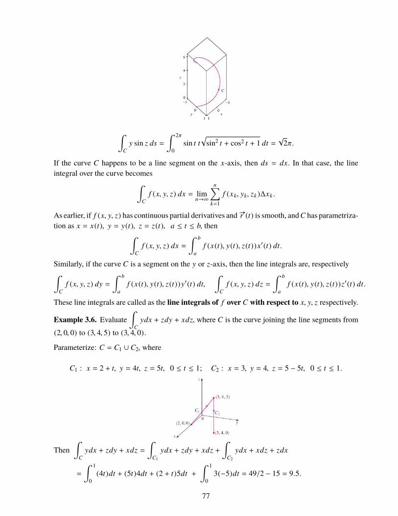
∫Cy sin z ds =

∫ 2π

0sin t t

√sin2 t + cos2 t + 1 dt =

√2π.

If the curve C happens to be a line segment on the x-axis, then ds = dx. In that case, the lineintegral over the curve becomes∫

Cf (x, y, z) dx = lim

n→∞

n∑k=1

f (xk, yk, zk )∆xk .

As earlier, if f (x, y, z) has continuous partial derivatives and #»r (t) is smooth, andC has parametriza-tion as x = x(t), y = y(t), z = z(t), a ≤ t ≤ b, then∫

Cf (x, y, z) dx =

∫ b

af (x(t), y(t), z(t))x′(t) dt.

Similarly, if the curve C is a segment on the y or z-axis, then the line integrals are, respectively∫C

f (x, y, z) dy =∫ b

af (x(t), y(t), z(t))y′(t) dt,

∫C

f (x, y, z) dz =∫ b

af (x(t), y(t), z(t))z′(t) dt.

These line integrals are called as the line integrals of f over C with respect to x, y, z respectively.

Example 3.6. Evaluate∫

Cydx + zdy + xdz, where C is the curve joining the line segments from

(2, 0, 0) to (3, 4, 5) to (3, 4, 0).

Parameterize: C = C1 ∪ C2, where

C1 : x = 2 + t, y = 4t, z = 5t, 0 ≤ t ≤ 1; C2 : x = 3, y = 4, z = 5 − 5t, 0 ≤ t ≤ 1.

Then∫

Cydx + zdy + xdz =

∫C1

ydx + zdy + xdz +∫

C2

ydx + xdz + zdx

=

∫ 1

0(4t)dt + (5t)4dt + (2 + t)5dt +

∫ 1

03(−5)dt = 49/2 − 15 = 9.5.

77

3.2 Line Integral of Vector FieldsWe want to generalize line integrals to vector fields.A vector field is a function defined on a region D in the plane or space that assigns a vector to eachpoint in D. If D is a region in space, a vector field on D may be written as

#»F (x, y, z) = M (x, y, z) ı + N (x, y, z) + P(x, y, z) k .

Vectors in a gravitational field point toward the center of mass that gives the source of the field.The velocity vectors on a projectile’s motion make a vector field along the trajectory.

Let #»F (x, y, z) be a continuous vector field defined over a curve C given by

#»r (t) = x(t) ı + y(t) + z(t) k for a ≤ t ≤ b.

The line integral of #»F along C, also called the work done by moving a particle on C under the

force field #»F is ∫

C

#»F · d #»r =

∫C

#»F ( #»r (t)) · #»r ′(t) dt =

∫C

#»F ·

#»T ds,

where #»T (t) =

#»r ′(t)| #»r ′(t) |

is the unit tangent vector at a point on C.

Example 3.7. Evaluate the line integral of the vector field #»F (x, y, z) = x2 ı − xy along the first

quarter unit circle in the first quadrant.

The curve C is given by #»r (t) = cos t ı + sin t , 0 ≤ t ≤ π/2. Then

#»F ( #»r (t)) = cos2 t ı − cos t sin t , #»r ′ = − sin t ı + cos t .

The work done is ∫C

#»F · d #»r =

∫ π/2

0

#»F ( #»r ) · #»r ′ dt =

−23.

78

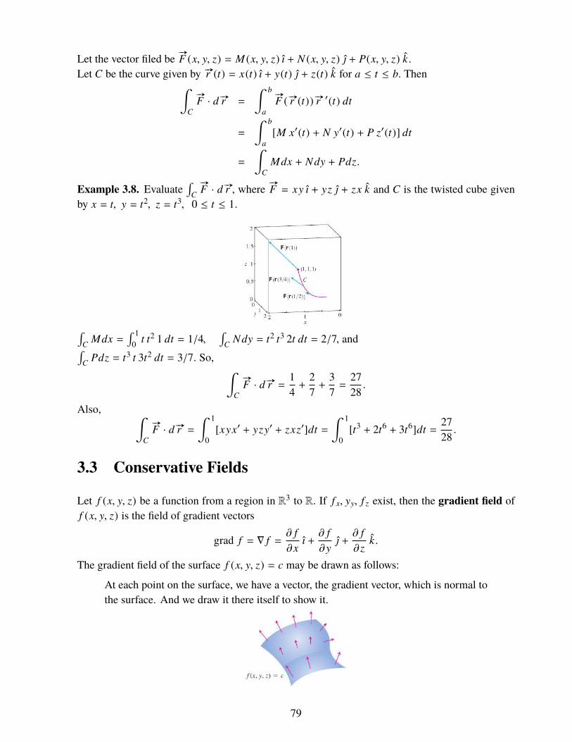
Let the vector filed be #»F (x, y, z) = M (x, y, z) ı + N (x, y, z) + P(x, y, z) k .

Let C be the curve given by #»r (t) = x(t) ı + y(t) + z(t) k for a ≤ t ≤ b. Then∫C

#»F · d #»r =

∫ b

a

#»F ( #»r (t)) #»r ′(t) dt

=

∫ b

a[M x′(t) + N y′(t) + P z′(t)] dt

=

∫C

Mdx + Ndy + Pdz.

Example 3.8. Evaluate∫

C#»F · d #»r , where #»

F = xy ı + yz + zx k and C is the twisted cube givenby x = t, y = t2, z = t3, 0 ≤ t ≤ 1.

∫C Mdx =

∫ 10 t t2 1 dt = 1/4,

∫C Ndy = t2 t3 2t dt = 2/7, and∫

C Pdz = t3 t 3t2 dt = 3/7. So, ∫C

#»F · d #»r =

14+

27+

37=

2728.

Also, ∫C

#»F · d #»r =

∫ 1

0[xyx′ + yzy′ + zxz′]dt =

∫ 1

0[t3 + 2t6 + 3t6]dt =

2728.

3.3 Conservative Fields

Let f (x, y, z) be a function from a region in R3 to R. If f x, yy, f z exist, then the gradient field off (x, y, z) is the field of gradient vectors

grad f = ∇ f =∂ f∂x

ı +∂ f∂y

+∂ f∂z

k .

The gradient field of the surface f (x, y, z) = c may be drawn as follows:

At each point on the surface, we have a vector, the gradient vector, which is normal tothe surface. And we draw it there itself to show it.

79

For example, the gradient field of f (x, y, z) = xyz is

grad f = yz ı + zx + xy k .

Notice that f (x, y, z) has a continuous gradient iff f x, f y, f z are continuous on the domain ofdefinition of f .

A vector field #»F is called conservative if there exists a scalar function f such that #»

F = grad f .In such a case, the scalar function f is called the potential of the vector field #»

F .

For example, consider the gravitational force field #»F = −

mMG|r |3

#»r . It is also written in the form:

#»F (x, y, z) = −

mMG(x2 + y2 + z2)3/2 [x ı + y + z k]

Here, #»F is a conservative field. Reason?

Define f (x, y, z) =mMG

(x2 + y2 + z2)1/2 . Then

grad f =∂ f∂x

ı +∂ f∂y

+∂ f∂z

k =#»F .

Physically, the law of conservation of energy holds in every conservative field.

Recall:∫ b

a f ′(t)dt = f (b) − f (a) for a function f (t). In case of line integrals, the gradient acts asa sort of derivative.

Theorem 3.2. Let C be a smooth curve given by #»r (t) = x(t) ı + y(t) + z(t) k for a ≤ t ≤ b.Suppose C joins points (x1, y1, z1) to (x2, y2, z2). That is,

#»r (a) = x1 ı + y1 + z1 k and #»r (b) = x2 ı + y2 + z2 k .

Let f (x, y, z) be a function whose gradient vector is continuous on a region containing C. Then∫C∇ f · d #»r = f ( #»r (b)) − f ( #»r (a)) = f (x2, y2, z2) − f (x1, y1, z1).

Proof:∫C∇ f · d #»r =

∫ b

a∇ f ( #»r (t)) · #»r ′(t) dt

=

∫ b

a

[∂ f∂x

dxdt+∂ f∂y

dydt+∂ f∂z

dzdt

]dt

=

∫ b

a

ddt

f ( #»r (t)) dt = f ( #»r (t))���b

a= f ( #»r (b)) − f ( #»r (a)). �

Theorem 3.2 says that if #»F is a conservative vector field with potential f , then the line integral over

any smooth curve joining points A to B can be evaluated from the potential by:∫C

#»F · d #»r = f (B) − f (A).

80

In such a case, the line integral is independent of path of C; it only depends on the initial point andthe end point of C.

We say that a line integral∫

C#»F · d #»r is independent of path iff for any curve C′ that is lying in

the domain of #»F, and having the same initial and end points as that of C, we have∫

C

#»F · d #»r =

∫C ′

#»F · d #»r .

Thus, if #»F is conservative, then the line integral

∫C

#»F · d #»r is path independent.

Example 3.9. Find the line integral of the field #»F = yz ı + zx + xy k along any smooth curve

joining the points A(−1, 3, 9) to B(1, 6,−4).

Notice that #»F is conservative since #»

F = grad (xyz) = ∇ f , where f = xyz. Let C be any suchcurve. Then ∫

C

#»F · d #»r =

∫ B

A∇ f · d #»r = f (B) − f (A) = 3.

The following result is a corollary to Theorem 3.2.

Theorem 3.3. Let #»F be a continuous vector field defined on a region D. Let C be any smooth curve

lying in D. The line integral∫

C#»F · d #»r is path independent iff

∫C ′

#»F · d #»r = 0 for every closed

curve C′ lying in D.

Remark: A closed curve is a curve having the same initial and end points. “Smooth curve” maybe replaced by “Piecewise smooth curve” everywhere. When C is a closed curve, the line integralover C is written as

∮C

#»F · d #»r .

Path independence implies that the field is conservative. We state this theorem without proof.

Theorem 3.4. Let #»F be a continuous vector field defined on a region D. If

∫C

#»F · d #»r is path

independent for each smooth curve C lying in D, then #»F is conservative.

If #»F (x, y) = M (x, y) ı + N (x, y) is conservative, then we have a scalar function f (x, y) such

that f x = M, f y = N . Then using Clairaut’s theorem, we have f xy = My = f yx = Nx . That is, if#»F = M ı + N is conservative, then My = Nx . Similar result holds in three dimensions.

Theorem 3.5. Let #»F (x, y, z) = M (x, y, z) ı + N (x, y, z) + P(x, y, z) k, where the gradients of the

component functions M, N, P are continuous on a region D. If #»F is conservative, then we have

My = Nx, Nz = Py, Px = Mz on D.

Example 3.10. Are the following vector fields conservative?

(a) #»F (x, y) = (x − y) ı + (x − 2)

(b) #»F (x, y) = (3 + 2xy) ı + (x2 − 3y2) .

(c) #»F (x, y, z) = (2x − 3) ı + z + cos z k .

81

(a) #»F = M ı + N , where M = x − y, N = x − 2. My = −1, Nx = 1. Since My , Nx, the vector

field F is not conservative.(b) Here, M = 3 + 2xy, N = x2 − 3y2. My = 2x = Nx . The vector filed is defined on R2, which isa simply connected region. The partial derivatives of M and N are continuous. Therefore, #»

F is aconservative field.(c) #»

F = M ı + N + P k, where M = 2x − 3, N = z, P = cos z.My = 0, Nx = 0, Nz = 1, Py = 0, Px = 0, Mz = 0.Since Nz , Py, the field

#»F is not conservative.

The converse of Theorem 3.5 holds if the region of #»F is a simply connected region.

A simple curve is a curve which does not intersect itself. A connected region D is said to be asimply connected region iff every simple closed curve lying in D encloses only points from D.

Theorem 3.6. Let #»F = M ı + N + P k be a vector field on a simply connected region D, where

gradients of M, N, P are continuous. If My = Nx, Nz = Py, and Px = Mz hold on D, then #»F is

conservative.

Proof of this can be done here, but it follows from Green’s theorem in the plane and from Stokes’theorem in space, which we will do later.These equations help in determining the potential function of a conservative field.

Example 3.11. Find a potential for the vector field #»F = (3 + 2xy) ı + (x2 − 3y2) . Then evaluate∫

C#»F · d #»r , where C is given by #»r (t) = et sin t ı + et cos t , 0 ≤ t ≤ π.

To determine a scalar function f (x, y, z) such that #»F = grad f , we start with

f x = 3 + 2xy, f y = x2 − 3y2.

Integrate the first one with respect to x and integrate the second with respect to y to obtain:

f (x, y) = 3x + x2y + g(y), f (x, y) = x2y − y3 + h(x).

Taking g(y) = −y3 + const. and h(x) = 3x + const., we have

f (x, y) = 3x + x2y − y3 + k for any constant k .

Verify to see that f is a potential for F.Next,

∫C

#»F · d #»r = f (x(π), y(π)) − f (x(0), y(0)) = e3π + 1.

82

Example 3.12. Find a potential for the vector field #»F = y2 ı + (2xy + e3z) + 3ye3z k .

Denote the potential by f (x, y, z). Then

f x = y2, f y = 2xy + e3z, f z = 3ye3z .

Integrate with respect to suitable variables:

f = xy2 + g(y, z), f = xy2 + ye3z + h(x, z), f = ye3z + φ(x, y).

Taking g(y, z) = ye3z, φ(x, y) = xy2, h(x, z) = k, a constant, we get one such f .

Sometimes matching may not be obvious. So, differentiate the first:

f y = 2xy + gy (y, z) = 2xy + e3z .

Thus, gy (y, z) = e3z . Integrate: g(y, z) = ye3z + ψ(z). Then

f = xy2 + ye3z + ψ(z).

This gives f z = 3e3z + ψ′(z) = 3y3z . Thus, ψ(z) = k, a const. Therefore,

f (x, y, z) = xy2 + ye3z + k .

Example 3.13. Show that the vector field #»F = (ex cos y + yz) ı + (xz − ex sin y) + (xy + z) k is

conservative by finding a potential for it.

Let the potential be f (x, y, z). Then

f x = ex cos y + yz, f y = xz − ex sin y, f z = xy + z.

Integrate the first w.r.t. x to get

f = ex cos y + xyz + g(y, z).

Differentiate w.r.t. y to get

f y = −ex sin y + xz + gy (y, z) = xz − ex sin y ⇒ gy (y, z) = 0.

Thus g(y, z) = h(z). And then f = ex cos y + xyz + h(z). Differentiate w.r.t. z to obtain

f z = xy + h′(z) = xy + z ⇒ h′(z) = z ⇒ h(z) = z2/2 + k .

Then f (x, y, z) = ex cos y + xyz + z2/2 + k .

If M, N, P are functions of x, y, z, on a region D in space, then the expression

M (x, y, z)dx + N (x, y, z)dy + P(x, y, z)dz

Is called a differential form. The differential form is called exact iff there exists a functionf (x, y, z) such that

M (x, y, z) =∂ f∂x, N (x, y, z) =

∂ f∂y, P(x, y, z) =

∂ f∂z.

83

Notice that if the differential form is exact, then

M (x, y, z)dx + N (x, y, z)dy + P(x, y, z)dz = df ,

which is an exact differential. In that case, if C is any curve joining points A to B in the region D,then ∫ B

A[Mdx + Ndy + Pdz] =

∫C∇ f · d #»r =

∫ B

Adf = f (B) − f (A).

Therefore, the differential form is exact iff #»F = M ı + N + P k is conservative. Then the scalar

function f (x, y, z) is the potential of the field #»F .

Example 3.14. Show that the differential form ydx + xdy + 4dz is exact. Then evaluate theintegral

∫C (ydx + xdy + 4dz) over the line segment C joining the points (1, 1, 1) to (2, 3,−1).

M = y, N = x, P = 4. Then My = 1 = Nx, Nz = 0 = Py, Px = 0 = Mz .

Therefore, the differential form is exact.Also, notice that ydx + xdy + 4dz = d(xy + 4z + k). Hence it is exact.In case, f is not obvious, we can determine it as earlier by differentiating and integrating etc. Next,∫

C(ydx + xdy + 4dz) =

∫ (2,3,−1)

(1,1,1)d(xy + 4z + k) = (xy + 4z + k)���

(2,3,−1)

(1,1,1)= −3.

3.4 Green’s TheoremLet C be a simple closed curve in the plane. The positive orientation of C refers to a singlecounter-clockwise traversal of C. If C is given by #»r (t), a ≤ t ≤ b, then its positive orientationrefers to a traversal of C keeping the region D bounded by the curve to the left.

Theorem 3.7. (Green’s Theorem) Let C be a positively oriented simple closed piecewise smoothcurve in the plane. Let D be the region bounded by C. (That is, C = ∂D.) If M (x, y) and N (x, y)have continuous partial derivatives on an open region containing D, then

1.∮

C(Mdx + Ndy) =

"D

(∂N∂x−∂M∂y

)dA.

2.∮

C(Mdy − Ndx) =

"D

(∂M∂x+∂N∂y

)dA.

84

Green’s theorem helps in evaluating an integral of the type∫ b

a#»F · d #»r in a non-conservative vector

field #»F . It gives a relationship between a line integral around a simple closed curve C and the

double integral over the plane region D bounded by this closed curve.

Proof: We only prove for a special kind of regions to give an idea of how it is proved.Consider the region D = {(x, y) : a ≤ x ≤ b, f (x) ≤ y ≤ g(x)}. Assume that f , g are continuousfunctions. Then"

D

∂M∂y

dA =∫ b

a

∫ g(x)

f (x)Mydydx =

∫ b

a[M (x, g(x)) − M (x, f (x))]dx.

Now we compute∫

C Mdx by breaking C into four parts C1,C2,C3 and C4.

The curve C1 is given by x = x, y = f (x), a ≤ x ≤ b. Thus∫C1

Mdx =∫ b

aM (x, f (x))dx.

On C2 and also on C4, the variable x is a single point. So,∫C2

Mdx =∫

C4

Mdx = 0.

As x increases, C3 is traversed backward. That is, −C3 is given by x = x, y = g(x), a ≤ x ≤ b. So,∫C3

Mdx = −∫

C3

Mdx = −∫ b

aM (x, g(x))dx.

Therefore,"

D

∂M∂y

dA = −∫

CMdx. Similarly, express D using the variable of integration as y.

Then we have"

D

∂N∂x

dA =∫

CNdy. Next, add the two results obtained to get

∫C

(Mdx + Ndy) ="

D

(∂N∂x−∂M∂y

)dA.

The second form follows similarly. �

Example 3.15. Verify Green’s theorem for the field #»F = (x − y) ı + x , where C is the unit circle

oriented positively.

85

Here, we have C : #»r (t) = x ı + y = cos t ı + sin t , 0 ≤ t ≤ 2π. The region D is the unit disk.

M = cos t − sin t, N = cos t, dx = − sin t dt, dy = cos t dt.

Mx = 1, My = −1, Nx = 1, Ny = 0.

Now, ∮C

(Mdy − Ndx) =∫ 2π

0[(cos t − sin t) cos t − cos t(− sin t)]dt = π."

D(Mx + Ny)dA =

"D

(1 + 0)dA = Area of D = π.

Similarly, ∮C

(Mdx + Ndy) =∫ 2π

0[(cos t − sin t)(− sin t) + cos2 t]dt = 2π."

D(Nx − My)dA =

"D

(1 − (−1))dA = 2 × Area of D = 2π.

Example 3.16. Evaluate the integral I =∮

C xy dy + y2 dx, where C is the square cut from the firstquadrant by the lines x = 1 and y = 1, with positive orientation.

Take M = y2, N = xy, D as the region bounded by C. Then

I =∮

C(Mdx + Ndy) =

"D

(Nx − My)dA =∫ 1

0

∫ 1

0(y − 2y)dxdy = −1/2.

Also, taking M = xy, and N = −y2, we have

I =∮

C(Mdy − Ndx) =

"D

(Mx + Ny)dA =∫ 1

0

∫ 1

0(y − 2y)dxdy = −1/2.

Example 3.17. Evaluate the integral I =∮

C (3y − esin x)dx + (7x +√

1 + y4)dy,

where C is the positively oriented circle x2 + y2 = 9.

Take D as the disk x2 + y2 ≤ 9. Then by Green’s theorem,

I ="

D

[(7x +

√1 + y4)x − (3y − esin x)y

]dA =

"D

(7 − 3)dA = 36π.

Example 3.18. Evaluate I =∮

C x4 dx + xy dy, where C is the triangle with vertices at (0, 0), (0, 1)and (1, 0); its orientation being from (0, 0) to (1, 0) to (0, 1) to (0, 0).

86

The triangle is positively oriented. Let D be the region bounded by the triangle.Take M = x4, N = xy. Then

I ="

D[(xy)x − (x4)y]dA =

∫ 1

0

∫ 1−x

0y dy dx =

12

∫ 1

0(1 − x2)dx =

16.

Example 3.19. Evaluate∫

C (xdy − y2dx), where C is the positively oriented square bounded bythe lines x = ±1 and y = ±1.

Here, M = x, N = y2, and D is the region bounded by C. By Green’s theorem,∮C

(Mdy − Ndx) ="

D(Mx + Ny)dA =

∫ 1

−1

∫ 1

−1(1 + 2y)dxdy = 4.

Observation: Consider the formula!

D (Nx − My)dA =∮

C (Mdx + Ndy).

1. Take M = 0 and N = x. Then Nx − My = 1 so that

Area of D ="

D(Nx − My)dA =

∮C

(Mdx + Ndy) =∮

Cxdy.

2. Take M = −y and N = 0. Then Nx − My = 1 so that

Area of D ="

D(Nx − My)dA =

∮C

(Mdx + Ndy) = −∮

Cydx.

3. Combining the two above, we also have

Area of D =12

∮C

(x dy − y dx).

For example, to compute the area enclosed by the ellipse C :x2

a2 +y2

b2 = 1, we parameterize C

as x = a cos t, y = b sin t, 0 ≤ t ≤ 2π. And then the area is

12

∮C

(x dy − y dx) =12

∫ 2π

0[(a cos t b cos t) − (b sin t (−b sin t))]dt =

12

∫ 2π

0ab dt = π ab.

Example 3.20. Evaluate∮

C (y2 dx + xy dy), where C is the boundary of the semi- annular regionbetween the semicircles x2 + y2 = 1 and x2 + y2 = 4 in the upper half plane.

87

Write, in polar coordinates, D = {(r, θ) : 1 ≤ r ≤ 2, 0 ≤ θ ≤ π}. Then∮C

(y2 dx + xy dy) ="

D

[ ∂∂x

(xy) −∂

∂y(y2)

]dA = −

"Dy dA

= −

∫ 2

1

∫ π

0r sin θr dr dθ = −

∫ 2

1r2dr

∫ π

0sin θ dθ = −

143.

In fact, Green’s theorem can be applied to regions having holes, provided the region can be dividedinto simply connected regions.

The boundary C of the region D consists of two simple closed curves C1 (Outer) and C2 (inner).Assume that these boundary curves are oriented so that the region D is always on the left as thecurve C is traversed.

Thus the positive direction is counterclockwise for the outer curve C1 but clockwise for the innercurve C2. Divide D into two regions D′ and D′′ as shown in the figure. Green’s theorem on D′ andD′′ gives"

D(Nx − My)dA =

"D′

(Nx − My)dA +"

D′′(Nx − My)dA

=

∫∂D′

(Mdx + Ndy) +∫∂D′′

(Mdx + Ndy) =∫

C(Mdx + Ndy).

This is the general version of Green’s Theorem.

Example 3.21. Show that ifC is any positively oriented simple closed path that encloses the origin,then ∮

C

−y

x2 + y2 dx +x

x2 + y2 dy = 2π,

No idea how to show it for every such curve. So, take a positively oriented circle C′, of radius a,around origin that lies entirely in the region bounded by C. Let D be the annular region boundedby C and C′. Take #»

F (x, y) = (−y ı + x )/(x2 + y2).

Then the positively oriented boundary of D is ∂D = C ∪ (−C′). Here, #»F = M ı + N gives

Nx = My = (y2 − x2)/(x2 + y2)2. Green’s theorem on D gives∮C

(Mdx + Ndy) +∮−C ′

(Mdx + Ndy) ="

D(Nx − My)dA = 0.

88

Then ∮C

(Mdx + Ndy) =∮

C ′(Mdx + Ndy).

But C′ is parameterized by x(t) = a cos t, y(t) = a sin t, 0 ≤ t ≤ 2π. So,∮C

(Mdx + Ndy) =∫

C ′(Mdx + Ndy) =

∫ 2π

0

#»F (a cos t ı+ a sin t ) · (a cos t ı+ a sin t )′dt = 2π.

Generalize this example by taking the constraint Nx = My on the vector field.

3.5 Curl and Divergence of a vector fieldIf #»

F = M ı + N + P k is a vector field in R3, where the partial derivatives of the componentfunctions exist, then curl #»

F is a vector field given by

curl #»F =

(∂P∂y−∂N∂z

)ı +

(∂M∂z−∂P∂x

) +

(∂N∂x−∂M∂y

)k .

Writing in operator notation, recall that grad = ∇ = ı∂

∂x+

∂

∂y+ k

∂

∂z.

Then curl #»F = ∇ ×

#»F =

��������

ı k∂∂x

∂∂y

∂∂z

M N P

��������.

For example, if #»F = zx ı + xyz − y2 k, then curl #»

F = −y(2 + x) ı + x + yz k .

Theorem 3.8. Let #»F be a vector field defined over a simply connected region D whose component

functions have continuous second order partial derivatives. Then #»F is conservative iff curl #»

F = 0.

Proof of⇒: If #»F is conservative, then #»

F = ∇ f for some f ,where f is some scalar function definedon D. Now,

curl ∇ f = ∇ × (∇ f ) =

��������

ı k∂∂x

∂∂y

∂∂z

f x f y f z

��������= ( f yz − f zy) ı + ( f zx − f xz) + ( f xy − f yx) k = 0.

The converse follows from Stokes’ theorem, which we will discuss later. �

Remember: The curl of gradient of any scalar function is zero:

curl grad f = 0.

Example 3.22. Is the vector field #»F = zx ı + xyz − y2 k conservative?

Here, curl #»F = −y(2 + x) ı + x + yz k , 0. So, #»

F is not conservative.

Example 3.23. Is the vector field #»F = y2z3 ı + 2xyz3 + 3xy2z2 k conservative?

89

Here, #»F is defined on R2 and

curl #»F =

��������

ı k∂∂x

∂∂y

∂∂z

y2z3 2xyz3 3xy2z2

��������=

(6xy2z2 − 6xy2z2) ı−(3y2z2 − 3y2z2) +(2yz3 − 2yz3) k

= 0.

Hence #»F is conservative. In fact, #»

F = grad f , where f (x, y, z) = xy2z3.

The name game: curl #»F measures how quickly a tiny peddle (at a point) in some fluid in a vector

field moves around itself. If curl #»F = 0, then there is no rotation of such a tiny peddle.

If #»F = M ı + N + P k is a vector field defined on a region, where its component functions have

first order partial derivatives, then

div #»F = ∇ ·

#»F =

∂M∂x+∂N∂y+∂P∂z

.

The divergence is also called flux or flux density.For example, if #»

F = zx ı + xyz − y2 k, then div #»F = z + xz.

The divergence of the vector field #»F = (x2 − y) ı + (xy − y2) is

∂(x2 − y)∂x

+∂(xy − y2)

∂y= 3x − 2y.

Intuitively, div #»F measures the tendency of the fluid to diverge from the point (a, b).When the gas

(fluid) is expanding, divergence is positive; and when it is compressing, the divergence is negative.The fluid is said to be incompressible iff div #»

F = 0.

Theorem 3.9. Let #»F = M ı + N + P k be a vector field defined on a simply connected region

D ⊆ R3, where M, N, P have continuous second order partial derivatives. Then div curl #»F = 0.

Proof: div curl #»F = ∇ · (∇ ×

#»F ) =

∂

∂x

(∂P∂y−∂N∂z

)+∂

∂y

(∂M∂z−∂P∂x

)+∂

∂z

(∂N∂x−∂M∂y

)This is equal to zero, due to Clairaut’s Theorem. �

Example 3.24. Does there exist a vector field G such that #»F = zx ı + xyz − y2 k = curl G?

div #»F = z + xz , 0. Hence there is no such G.

Divergence of grad f is the Laplacian of a scalar function f since

div grad f = ∇ · (∇#»F ) =

∂2 f∂x2 +

∂2 f∂y2 +

∂2 f∂z2 := ∇2 f .

The operator ∇2 = ∂2

∂x2 +∂2

∂y2 +∂2

∂z2 is called the Laplacian.

Green’s Theorem - Tangent formLet D be a simply connected region whose boundary is the simple closed curve C.Let #»

F = M ı + N be a vector field defined on D.

90

Let C be parameterized by #»r (t) = x(t) ı + y(t) .Let #»

T (t) be the unit tangent vector to C at the point (x(t), y(t)). Then

#»F ·

#»T (t)ds =

#»F · d #»r = Mdx + Ndy.

The line integral of #»F over C is∮

#»F ·

#»T (t)ds =

∮C

#»F · d #»r =

∮C

(M dx + N dy).

Consider #»F as a vector field on R3 with P = 0. Then

curl #»F = (Nx − My) k ⇒ curl #»

F · k = Nx − My .

Thus Green’s theorem takes the form∮C

#»F ·

#»T (t) ds =

∮C

#»F · d #»r =

"D

(curl #»F · k) dA.

Green’s Theorem - Normal formLet C be given by #»r (t) = x(t) ı + y(t) . Then

#»T =

x′(t)| #»r ′(t) |

ı +y′(t)| #»r ′(t) |

, n(t) =y′(t)| #»r ′(t) |

ı −x′(t)| #»r ′(t) |

.

Then #»F · n = [M y′(t) − N x′(t)]/| #»r ′(t) |.

Now,∮

C#»F · n ds =

∫ ba

#»F · n | #»r ′(t) | dt =

∮C (Mdy − Ndx).

Also,!

D div #»F dA =

!D (Mx + Ny)dA.

Hence Green’s theorem takes the form∮C

#»F · n ds =

"D

div #»F dA.

The tangent form of Green’s theorem is also called the circulation-curl form and the normal formis called flux-divergence form. Both the tangent form and the normal form of Green’s theorem aretogether referred to as vector forms of Green’s theorem.

3.6 Surface Area of solids of RevolutionSuppose a smooth curve is given by y = f (x), where f (x) ≥ 0. Its arc when a ≤ x ≤ b is revolvedabout the x-axis to generate a solid. How do we compute the area of the surface of this solid?We follow a strategy similar to computing the volume of revolution. Partition [a, b] into n subin-tervals [xk−1, xk]. When each ∆xk is small, the surface area corresponding to this subinterval isapproximately same as the area on the frustum of a right circular cone.

91

If a right circular cone has base radius R and slant height `, then its surface area is given by πR`.Now, for the frustum, we subtract the smaller cone surface area from the larger. Look at the figure.The area of the frustum is

A = πr2(`1 + `) − πr1`1 = π[(r2 − r1)`1 + r2`].

Using similarity of triangles, we have`1r1=`1 + `

r2.

This gives r2`1 = r1`1 + r1` ⇒ (r2 − r1)`1 = r1`. Therefore,

A = π(r1` + r2`) = 2π r `, where r =r1 + r2

2.

To use this this formula on the frustum obtained on the subinterval [xk−1, xk],we notice that the slantheight ` is approximated by

√(∆xk )2 + (∆yk )2,where∆xk = xk−xk−1 and∆yk = f (xk )− f (xk−1).

Next, the average radius r = r1+r22 is f (xk−1)+ f (xk )

2 . Thus the area of the frustum is

Ak = 2πf (xk−1) + f (xk )

2

√(∆xk )2 + (∆yk )2.

Due to MVT, we have ck ∈ [xk−1, xk] such that

∆yk = f (xk ) − f (xk−1) = f ′(ck )(xk − xk−1) = f ′(ck )∆xk .

So,√

(∆xk )2 + (∆yk )2 =√

1 + ( f ′(ck ))2 ∆xk . The surface of revolution is approximated byn∑

k=1Ak = 2π

f (xk−1) + f (xk )2

√1 + ( f ′(ck ))2 ∆xk .

Its limit as n → ∞ is the Riemann sum of an integral, which is the required area:

S =∫ b

a2π f (x)

√1 + ( f ′(x))2 dx =

∫ b

a2πy

√1 + ( f ′(x))2 dx.

We summarize.

1. If the arc of the curve y = f (x) for a ≤ x ≤ b is revolved about the x-axis, then writeds =

√1 + ( f ′(x))2dx. The area of the surface of the solid of revolution is given by

S =∫

2πy ds =∫ b

a2πy

√1 + ( f ′(x))2 dx.

92

2. If the arc of the curve x = g(y) for c ≤ y ≤ d is revolved about the y-axis, then writeds =

√1 + (g′(y))2 dy. The area of the surface of the solid of revolution is given by

S =∫

2πx ds =∫ d

c2πx

√1 + (g′(y))2 dy.

For parameterized curves, suppose the smooth curve is given by x = x(t), y = y(t) for a ≤ t ≤ b.If the curve is traversed exactly once while t increases from a to b, then the surface area of the solidgenerated by revolving the curve about the coordinate axes are as follows:

1. Revolution about the x-axis (y ≥ 0) : S =∫ b

a2π y(t)

√(x′(t))2 + (y′(t))2 dt.

2. Revolution about the y-axis (x ≥ 0) : S =∫ b

a2π x(t)

√(x′(t))2 + (y′(t))2 dt.

Example 3.25. Find the surface area of the solid obtained by revolving about x-axis, the arc of thecurve y = 2

√x, 1 ≤ x ≤ 2.

Since y = 2√

x, y′ = 1/√

x,√

1 + (y′)2 =√

1 + 1/x. Then

S =∫ 2

12πy

(1 + [y′]2

)1/2dx =

∫ 2

12π 2√

x

√1 +

1x

dx =8π3

(3√

3 − 2√

2).

Example 3.26. The arc of the parabola y = x2, 1 ≤ x ≤ 2 is revolved about the y-axis. Find thesurface area of revolution.

Since y′ = 2x, the surface area is

S =

∫ 2

12π x

√1 + (y′)2 dx = 2π

∫ 2

1x√

1 + 4x2 dx

= π ·23·

14

∫ 2

1

√1 + 4x2 d(1 + 4x2) =

π

6[1 + 4x2

]2

1=π

6(17√

17 − 5√

5)

93

Example 3.27.

The circle of radius 1 centered at (0, 1) is revolved aboutthe x-axis. Find the surface area of the solid so generated.The circle can be parameterized as

x = cos t, y = 1 + sin t, 0 ≤ t ≤ 2π.

Then (x′(t))2 + (y′(t))2 = 1. Thus the area is

S =∫ 2π

02π (1 + sin t) dt = 4π2.

3.7 Surface areaAs we know, smooth surfaces can be given by a function such as z = f (x, y). More generally,a smooth surface is given parametrically by x = x(u, v), y = y(u, v), z = z(u, v), where (u, v)varies over a given parameter region. Normally, we say that the point (u, v) varies over a region inuv-plane. The parametric equation is also written in vector form as

#»r = x(u, v)ı + y(u, v) + z(u, v) k .

Some examples:

The cone z =√

x2 + y2, 0 ≤ z ≤ 1 can be parametrized by

x = r cos θ, y = r sin θ, z = r, where 0 ≤ r ≤ 1 and 0 ≤ θ ≤ 2π.

Then its vector form is#»r (r, θ) = r cos θ ı + r sin θ + r k .

The sphere x2 + y2 + z2 = a2 can be parametrized by

x = a cos θ sin φ, y = a sin θ sin φ, z = a cos φ for 0 ≤ θ ≤ 2π, 0 ≤ φ ≤ π.

In vector form the parametrization is

#»r (θ, φ) = a cos θ sin φ ı + a sin θ sin φ + a cos φ k .

The cylinder x2 + y2 = a2, 0 ≤ z ≤ 5 can be parametrized by

#»r (θ, z) = a cos θ ı + a sin θ + z k, for 0 ≤ θ ≤ 2π.

Let S be a smooth surface given parametrically by x = x(u, v), y = y(u, v), z = z(u, v), where(u, v) ranges over a parameter region D in the uv-plane. Suppose that S is covered exactly once as(u, v) varies over D. For simplicity, assume that D is a rectangle. We write S in vector form:

#»r = x(u, v)ı + y(u, v) + z(u, v) k .

94

Divide D into smaller rectangles Ri j with the lower left corner point as Pi j = (ui, v j ). For simplicity,let the partition be uniform with u-lengths as ∆u and v-lengths as ∆v. The part Si j of S thatcorresponds to Ri j has the corner Pi j with position vector #»r (ui, v j ). The tangent vectors to S at Pi j

are given by#»r ∗u := #»r u(ui, v j ) = xu(ui, v j )ı + yu(ui, v j ) + zu k (ui, v j )#»r ∗v := #»r v (ui, v j ) = xv (ui, v j )ı + yv (ui, v j ) + zv k (ui, v j )

The tangent plane to S is the plane that contains the two tangent vectors #»r u(ui, v j ) and #»r v (ui, v j ).The normal to S at Pi j is the vector #»r u(ui, v j ) × #»r v (ui, v j ). Notice that since S is assumed to besmooth, the normal vector is non-zero.The part Si j is a curved parallelogram on S whose sides can be approximated by the vectors #»r ∗u∆uand #»r ∗v∆v. Then the area of Si j can be approximated by

Area of Si j ' |#»r ∗u ×

#»r ∗v |∆u∆v.

Then an approximation to the area of S is obtained by summing over both indices i and j:

Area of S '∑

j

∑i

| #»r ∗u ×#»r ∗v |∆u∆v.

We thus define the surface area by taking the limit of the above approximated quantity. It is asfollows:Let S be a smooth surface given parametrically by

#»r = x(u, v)ı + y(u, v) + z(u, v) k,

where (u, v) ∈ D, a region in the uv-plane. Suppose that S is covered exactly once as (u, v) variesover D. Then the surface area of S is given by

Area of S ="

D| #»r u ×

#»r v | dA

where #»r u = xuı + yu + zu k and #»r v = xv ı + yv + zv k .

In case, the surface S is given by the graph of a function such as z = f (x, y), where (x, y) ∈ D,then we take the parameters as u = x, v = y and z = z(u, v) = f (x, y). That is, S is given by

#»r = uı + v + zk .

95

We see that#»r u = ı + zu k = ı + f x k, #»r v = + zv k = + f y k .

#»r u ×#»r v =

��������

ı k1 0 f x

0 1 f y

��������= − f x ı − f y + k .

Therefore,Area of S =

"D| #»r u ×

#»r v | dA ="

D

√f 2

x + f 2y + 1 dA.

This formula can also be derived from the first principle as we had done for the parametric form.For this, suppose that S is given by the equation z = f (x, y) for (x, y) ∈ D. Divide D into smallerrectangles Ri j with area ∆(Ri j ) = ∆x∆y. For the corner (xi, y j ) in Ri j, closest to the origin, let Pi j

be the point (xi, y j, f (xi, y j )) on the surface. The tangent plane to S at Pi j is an approximation toS near Pi j .

The area Ti j of the portion of the tangent plane that lies above Ri j approximates the area of Si j, theportion of S that is directly above Ri j . Therefore, we define the area of the surface S as

∆(S) = limm→∞

limn→∞

m∑i=1

n∑j=1

Ti j .

Let #»a and #»

b be the vectors that start at Pi j and lie along the sides of the parallelogram whose areais Ti j . Then Ti j = |

#»a ×#»

b |. However, f x (xi, y j ) and f y (xi, y j ) are the slopes of the tangent linesthrough Pi j in the directions of #»a and #»

b , respectively. Therefore,

#»a = ∆x ı + f x (xi, y j )∆x k,#»

b = ∆y + f y (xi, y j )∆y k .

Ti j = | #»a ×#»

b | = | − f x (xi, y j ) ı − f y (xi, y j ) + k | ∆(Ri j )

=

√f 2

x (xi, y j ) + f 2y (xi, y j ) + 1 ∆(Ri j ).

Summing over these Ti j and taking the limit, we obtain:

Area of S ="

D

√f 2

x + f 2y + 1 dA.

Example 3.28. Find the surface area of the part of the surface z = x2 + 2y that lies above thetriangular region in the xy-plane with vertices (0, 0), (1, 0) and (1, 1).

96

T = {(x, y) : 0 ≤ x ≤ 1, 0 ≤ y ≤ x}, f (x, y) = x2 + 2y.

The required surface area is"T

√(2x)2 + 22 + 1 dA =

∫ 1

0

∫ x

0

√4x2 + 5 dydx =

112

(27 − 5√

5).

Surface Area - a generalized form

Recall that for a surface S which is given by f (x, y) = z, the surface area is"

D

√f 2

x + f 2y + 1dA.

Here, D is the rectangle on the xy-plane obtained by projecting S onto the plane.Look at this surface as f (x, y) − z = 0. Then ∇ f = f x ı + f y − 1 k . If #»p is the unit normal to theprojected rectangle, then #»p = k . Then

|∇ f ||∇ f · #»p |

=

√f 2

x + f 2y + 1

12 ,

which is the integrand in the surface area formula.Warning: ∇ f · #»p must not be ZERO.A derivation similar to the surface area formula gives the following:Let the surface S be given by f (x, y, z) = c. Let R be a closed bounded region which is obtainedby projecting the surface to a plane whose unit normal is #»p . Suppose that ∇ f is continuous on Rand ∇ f · #»p , 0 on R. Then

The surface area of S ="

R

|∇ f ||∇ f · #»p |

dA.

Of course, whenever possible, we project onto the coordinate planes.

Example 3.29. Find the area of the surface cut from the bottom of the paraboloid x2 + y2 = z bythe plane z = 4.

97

Surface S is given by f (x, y, z) = x2 + y2 − z = 0. Project it onto xy-plane to get the region R asx2 + y2 ≤ 4. Then ∇ f = 2x ı + 2y − k . |∇ f | =

√1 + 4x2 + 4y2.

#»p = k . |∇ f · #»p | = 1.

R is given by x = r cos θ, y = r sin θ, 0 ≤ θ ≤ 2π, 0 ≤ r ≤ 2. So, the surface area is"R

√1 + 4x2 + 4y2 dA =

∫ 2π

0

∫ 2

0

√1 + 4r2 r drdθ =

π

6(17√

17 − 1).

Example 3.30. Find the surface area of the cap cut from the hemisphere x2 + y2 + z2 = 2, z ≥ 0by the cylinder x2 + y2 = 1.

The surface projected on xy-plane gives R as the disk x2 + y2 ≤ 1. The surface is f (x, y, z) = 2,where f (x, y, z) = x2 + y2 + z2. Then

∇ f = 2x ı + 2y + 2z k, |∇ f | = 2√

x2 + y2 + z2 = 2√

2.

#»p = k . |∇ f · #»p | = |2z | = 2z. Thus the surface area is

∆ =

"R

2√

22z

dA =√

2"

Rz−1 dA =

√2"

R(2 − x2 − y2)−1/2 dA.

R is given by x = r cos θ, y = r sin θ, 0 ≤ θ ≤ 2π, 0 ≤ r ≤ 1. So,

∆ =√

2∫ 2π

0

∫ 1

0

r dr dθ√

2 − r2= 2π(2 −

√2).

98

3.8 Integrating over a surfaceSuppose a function g(x, y, z) is defined over a surface S given by f (x, y, z) = c. To compute theintegral of g, where the area elements are taken over the surface, we look at the region R on whichthis surface is defined as a function. Divide the region R into smaller rectangles ∆Ak . Consider thecorresponding surface areas ∆σk .

Then ∆σk ≈( |∇ f ||∇ f · #»p |

)k∆Ak . Assuming that g is nearly constant on the smaller surface frag-

ment σk, we form the sum∑k

g(xk, yk, zk )∆σk ≈ g(xk, yk, zk )( |∇ f ||∇ f · #»p |

)k∆Ak .

If this sum converges to a limit, then we define that limit as the integral of g over the surface S.

Let S be a surface S given by f (x, y, z) = c. Let the projection of S onto a plane with unit normal#»p be the region R. Let g(x, y, z) be defined over S. Then the surface integral of g over S is"

Sg dσ =

"Rg(x, y, z)

|∇ f ||∇ f · #»p |

dA.

Also, we write the surface differential as

dσ =|∇ f ||∇ f · #»p |

dA.

Warning: |∇ f · #»p | must not be ZERO.If the surface S can be represented as a union of non-overlapping smooth surfaces S1, . . . , Sn, then"

Sg dσ =

"S1

g dσ + · · · +"

Sng dσ.

If g(x, y, z) = g1(x, y, z) + · · · + gm(x, y, z) over the surface S, then"Sg dσ =

"Sg1 dσ + · · · +

"Sgm dσ.

Similarly, if g(x, y, z) = k h(x, y, z) holds for a constant k, over S, then"Sg(x, y, z) dσ =

"S

k h(x, y, z) dσ.

99

Example 3.31. Integrate g(x, y, z) = xyz over the surface of the cube cut from the first octant bythe planes x = 1, y = 1, and z = 1.

We integrate g over the six surfaces and add the results. As g = xyz is zero on the coordinateplanes, we need integrals on sides A, B and C.

Side A is the surface defined on the region RA : 0 ≤ x ≤ 1, 0 ≤ y ≤ 1 on the xy-plane. For thissurface and the region,

#»p = k, ∇ f = k, |∇ f | = 1, |∇ f · #»p | = | k · k | = 1, g(x, y, z) = xyz��z=1 = xy.

Therefore, "Ag(x, y, z) dσ =

"R1

xy|∇ f ||∇ f · #»p |

dA =∫ 1

0

∫ 1

0xydxdy =

∫ 1

0

y

2=

14.

Similarly, "Bg(x, y, z) dσ =

14=

"Cg(x, y, z) dσ.

Thus,"

Sg dσ =

34.

Example 3.32. Evaluate the surface integral of g(x, y, z) = x2 over the unit sphere.

S can be divided into the upper hemisphere and the lower hemisphere. Let S be the upper hemispheref (x, y, z) := x2 + y2 + z2 = 1, z ≥ 0. Its projection on the xy-plane is the region

R : x = r cos θ, y = r sin θ, 0 ≤ r ≤ 1, 0 ≤ θ ≤ 2π.

Here,#»p = k, |∇ f | = 2

√x2 + y2 + z2 = 2,

|∇ f · #»p | = 2|z | = 2√

1 − (x2 + y2) = 2√

1 − r2.

Hence "S

x2 dσ =

"R

x2 |∇ f ||∇ f · #»p |

dA ="

R

x2√

1 − r2dA

=

∫ 2π

0

∫ 1

0

r2 cos2 θ√

1 − r2r dr dθ

∫ 2π

0cos2 θ dθ

∫ 1

0

r3√

1 − r2dr =

2π3.

100

Since the integral of x2 on the upper hemisphere is equal to that on the lower hemisphere, therequired integral is 2 ×

2π3=

4π3.

Recall that when #»p = k, that is, when the region R is obtained by projecting the surface S onto thexy-plane,

|∇ f ||∇ f · #»p |

=

√1 + z2

x + z2y . Now, if the surface f (x, y, z) = c can be written explicitly by

z = h(x, y), then the surface integral takes the form"Sg(x, y, z) dσ =

"Rg(x, y, h(x, y))

√1 + h2

x + h2y dx dy.

Similarly, if the surface can be written as y = h(x, z) and R is obtained by projecting S onto thexz-plane, then "

Sg(x, y, z) dσ =

"Rg(x, h(x, z), z)

√1 + h2

x + h2z dx dz.

If the surface can be written as x = h(y, z) and R is obtained by projecting S onto the yz-plane,then "

Sg(x, y, z) dσ =

"Rg(h(y, z), y, z)

√1 + h2

y + h2z dy dz.

Example 3.33. Evaluate!

S y dσ, where S is the surface z = x + y2, 0 ≤ x ≤ 1, 0 ≤ y ≤ 2.

Projecting the surface onto xy-plane, we obtain the region R as the rectangle

R : 0 ≤ x ≤ 1, 0 ≤ y ≤ 2.

Here, the surface is given by z = h(x, y) = x + y2. So,"Sy dσ =

"Ry

√1 + 1 + (2y)2 dA =

∫ 1

0

∫ 2

0

√2y

√(1 + 2y2) dy dx =

13√

23

.

Suppose the surface S is given in a parameterized form:

#»r (u, v) = x(u, v) ı + y(u, v) + z(u, v) k,

where (u, v) ranges over the region D in the uv-plane. Here, a change of variable happens. TheJacobian is simply #»r u ×

#»r v . Then

dσ = | #»r u ×#»r v | dA,

where #»r u = xu ı + yu + zu k and #»r v = xv ı + yv + zv k . Then"S

f (x, y, z) dσ ="

Df ( #»r (u, v)) | #»r u ×

#»r v | dA.

101

Also this formula can directly be derived as we had done for computing surface area when a surfaceis given parametrically. It is as follows.Suppose the smooth surface S has the parametric equation in vector form as

#»r = x(u, v)ı + y(u, v) + z(u, v) k .

Assume that the parameter region D is a rectangle. Divide D into smaller rectangles Ri j by takinggrid lengths ∆u and ∆v.

Then the surface S is divided into corresponding patches Si j . We evaluate f at a point Pi j in Si j

and form the Riemann sum∑

i∑

j f (Pi j )∆Si j, where ∆Si j is the area of the patch Si j . Taking limitas the number of sub-rectangles approach∞, we obtain the surface integral of f over S as"

Sf (x, y, z) dσ = lim

m→∞limn→∞

n∑i=1

m∑j=1

f (Pi j )∆Si j .

However, ∆Si j = |#»r u(Pi j ) × #»r v (Pi j ) |∆u∆v. Therefore, the surface integral is given by"

Sf (x, y, z) dσ =

"D

f ( #»r (u, v)) | #»r u ×#»r v | dA.

Observe that the surface area of S is simply!

S 1 dσ as it should be. The relation between a surfaceintegral and surface area is much the same as that between a line integral and the arc length of acurve.

Example 3.34. Evaluate!

S z dσ, where S is the surface whose sides S1 are given by the cylinderx2+ y2 = 1, bottom S2 is the disk x2+ y2 ≤ 1, z = 0, and whose top S3 is part of the plane z = 1+ xthat lies above S2.

102

S1 is given by #»r = x ı+ y + z k with x = cos θ, y = sin θ, z = z, where D is given by 0 ≤ θ ≤ 2πand 0 ≤ z ≤ 1 + x = 1 + cos θ. Then

| #»r θ ×#»r z | = | cos θ ı + sin θ | = 1;"

S1

z dσ ="

Dz | #»r θ ×

#»r z | dA =∫ 2π

0

∫ 1+cos θ

0z dz dθ =

∫ 2π

0

(1 + cos θ)2

2dθ =

3π2.

S2 lies in the plane z = 0. Hence!

S2z dσ = 0.

S3 lies above the unit disk and lies in the plane z = 1 + x.Here, u = x, v = y and #»r = xı + y + z(x, y) . Then

| #»r u ×#»r v | = |(ı + zx k) × ( + zy k) | =

√z2

x + z2y + 1.

So, "S3

z dσ =

"D

(1 + x)√

1 + z2x + z2

y dA

=

∫ 2π

0

∫ 1

0(1 + r cos θ)

√1 + 1 + 0 r dr dθ =

√2π.

Hence, "S

z dσ ="

S1

z dσ +"

S2

z dσ +"

S3

z dσ =3π2+√

2π.

3.9 Surface Integral of a Vector FieldA smooth surface is called orientable iff it is possible to define a vector field of unit normal vectorsn to the surface which varies continuously with position. Once such normal vectors are chosen, thesurface is considered an oriented surface.

If the surface S is given by z = f (x, y), then we take its orientation by considering the unit normal

vectors n =− f x ı − f y + k√

1 + f 2x + f 2

y

.

If S is a part of a level surface g(x, y, z) = c, then we may take n =∇g

|∇g |.

If S is given parametrically as #»r (u, v) = x(u, v) ı + y(u, v) + z(u, v) k, then n =#»r u ×

#»r v

| #»r u ×#»r v |

.

Sometimes we may take negative sign if it is preferred. Conventionally, the outward direction istaken as the positive direction.

103

Let #»F be a continuous vector field defined over an oriented surface S with unit normal n. The

surface integral of #»F over S, also called, the flux of #»

F across S is"S

#»F · n dσ.

The flux is the integral of the scalar component of #»F along the unit normal to the surface. Thus

in a flow, the flux is the net rate at which the fluid is crossing the surface S in the chosen positivedirection.

If S is part of a level surface g(x, y, z) = c,which is defined over the region D, then dσ =|∇g |

|∇g. #»p |dA.

So, the flux across S is"S

#»F · n dσ =

"S

#»F ·±∇g

|∇g |dσ =

"D

#»F ·

±∇g

|∇g · #»p |dA.

If S is parametrized by #»r (u, v), where D is the region in uv-plane, thendσ = | #»r u ×

#»rv | du dv. So, flux across S is"S

#»F · n dσ =

"S

#»F ·

#»r u ×#»rv

| #»r u ×#»rv |

dσ ="

D

#»F ( #»r (u, v)) · ( #»r u ×

#»rv ) du dv.

Example 3.35. Find the flux of #»F = yz + z2 k outward through the surface S which is cut from

the cylinder y2 + z2 = 1, z ≥ 0 by the planes x = 0 and x = 1.

S is given by g(x, y, z) := y2 + z2 − 1 = 0, defined over the rectangle R = Rxy as in the figure.

The outward unit normal is n = +∇g

|∇g |= y + z k .

Here, #»p = k . So, dσ =|∇g |

|∇g · k |dA =

√y2 + z2

z=

1z

dA.

#»F · n on S is y2z + z3 = z(y2 + z2) = z. Therefore, outward flux through S is"

S

#»F · n dσ =

"R

z1z

dA ="

RdA = Area of R = 2.

Example 3.36. Find the flux of the vector field #»F = z ı + y + x k across the unit sphere.

If no direction of the normal vector is given and the surface is a closed surface, we take n in thepositive direction, which is directed outward.

104

Using the spherical coordinates, the unit sphere S is parametrized by

#»r (φ, θ) = sin φ cos θ ı + sin φ sin θ + cos φ k,

where 0 ≤ φ ≤ π and 0 ≤ θ ≤ 2π give the region D. Then#»F ( #»r (φ, θ)) = cos φ ı + sin φ sin θ + sin φ cos θ k .

#»r φ ×#»r θ = sin2 φ cos θ ı + sin2 φ sin θ + sin φ cos θ k .

Consequently,"S

#»F · #»n dσ =

"D

#»F · ( #»r φ ×

#»r θ ) dφ dθ

=

∫ 2π

0

∫ π

0(2 sin2 φ cos φ cos θ + sin2 φ sin2 θ) dφ dθ =

4π3.

Example 3.37. Find the surface integral of the vector field#»F = yz ı + x − z2 k

over the portion of the parabolic cylinder given by

y = x2, 0 ≤ x ≤ 1, 0 ≤ z ≤ 4.

We assume the positive direction of the normal n. Onthe surface, we have x = x, y = x2, z = z giving theparametrization as #»r (x, z) = x ı + x2 + z k where D isgiven by 0 ≤ x ≤ 1, 0 ≤ z ≤ 4.

On the surface #»F = x2z ı + x − z2 k . So,"

S

#»F · n dσ =

"D

#»F · ( #»r x ×

#»r z) dx dz

=

"D

(x2z ı + x − z2 k) · (2x ı − ) dx dz

=

∫ 4

0

∫ 1

0(2x3z − x) dx dz =

∫ 4

0

z − 12

dz = 2.

If S is given by z = f (x, y), then think of x, y as the parameters u and v.We have#»F = M (x, y) ı + N (x, y) + P(x, y) k and #»r = x ı + y + f (x, y) k .

Then #»r x ×#»r y = ( ı + f x k) × ( + f y k) = − f x ı − f y + k .

Therefore, the flux is"S

#»F · n dσ =

"D

#»F · ( #»r x ×

#»r y) dxdy ="

D(−M f x − N f y + P) dxdy.

Example 3.38. Evaluate!

S#»F · n dσ, where #»

F = y ı+ x + z k and S is the boundary of the solidenclosed by the paraboloid z = 1 − x2 − y2 and the plane z = 0.

105

The surface S has two parts: the top portion S1 and the base S2. Since S is a closed surface, weconsider its outward unit normal n. Projections of both S1 and S2 on xy-plane are D, the unit disk.By the simplified formula for the flux, we have"

S1

#»F · n dσ =

"D

(−M f x − N f y + P)dxdy

=

"D

[−y(−2x) − x(−2y) + 1 − x2 − y2]dxdy

=

∫ 2π

0

∫ 1

0(1 + 4r2 cos θ sin θ − r2) r dr dθ

=

∫ 2π

0

(14+ cos θ sin θ

)dθ =

π

2.

The disk S2 has positive direction, when n = − k . Thus"S2

#»F · n dσ =

"S2

(−#»F · k) dσ =

"D

(−z)dxdy = 0

since on D = S2, z = 0. Then"S

#»F · n dσ =

"S1

#»F · n dσ +

"S2

#»F · n dσ =

π

2.

3.10 Stokes’ TheoremConsider an oriented surface with a unit normal vector n. Call the boundary curve of S as C. Theorientation of S induces an orientation on C.

We say that C is positively oriented iff whenever you walk in the positive direction of C keepingyour head pointing towards n, S will be to your left.Recall that Green’s theorem relates a double integral in the plane to a line integral over its boundary.We will have a generalization of this to 3 dimensions. Write the boundary curve of a given smoothsurface as ∂S. The boundary is assumed to be a closed curve, positively oriented unless specifiedotherwise.

106

Theorem 3.10. (Stokes’ Theorem) Let S be an oriented piecewise-smooth surface that is boundedby a simple, closed, piecewise-smooth boundary curve ∂S with positive orientation.Let F = M ı+ N + P k be a vector field with M, N, P having continuous partial derivatives on anopen region in space that contains S. Then∮

∂S

#»F · d #»r =

"S

curl #»F · n dσ.

In particular, if S is a bounded region D in the xy-plane, ∂S = C, the smooth boundary of D, thenn = k and dσ = dA.We obtain∮

C

#»F · d #»r =

"D

curl #»F · k dA =

"D

(Nx − My) dx dy.

as Green’s theorem states. In fact, we can use Green’s theorem to prove Stokes’ theorem in case Sis the graph of a smooth function z = f (x, y) with a smooth boundary, and the vector field #»

F issmooth.

Proof: Let #»F = M ı + N + P k .We see that∮

∂S

#»F · d #»r =

∮∂S

M dx + N dy + P dz.

And "S

curl #»F · n dσ =

"S

curl (M ı) · n dσ

+

"S

curl (N ) · n dσ +"

Scurl (P k) · n dσ.

We show that the M-, N- and P- components in both are equal.Suppose S is given by z = f (x, y) for (x, y) ∈ D. Orient ∂D positively, i.e., counter-clock-wise.Choose a parameterization for this. Suppose ∂D is given by

#»r (t) = x(t) ı + y(t) for a ≤ t ≤ b.

Then ∂S has the parameterization as

#»r (t) = x(t) ı + y(t) + f (x(t), y(t)) for a ≤ t ≤ b.

107

Thus ∮∂S

M (x, y, z) dx =∫ b

aM (x(t), y(t), f (x(t), y(t))

dxdt

dt.

Or that ∮∂S

M (x, y, z) dx =∫∂D

M (x, y, z) dx.

Next, we apply Green’s theorem on the integral on the right to obtain:∮∂S

M (x, y, z) dx = −"

DMy (x, y, f (x, y)) dA.

Apply Chain rule on the right side integrand to obtain∮∂S

My (x, y, z) dx = −"

D

[My (x, y, f (x, y)) + Mz (x, y, f (x, y)) f y

]dA.

We now compute!

S curl (M ı)dσ. For this, notice that S has the parameterization:

#»r (t) = x(t) ı + y(t) + f (x, y) k .

So, n =− f x ı − f y + k

c, where c = | − f x ı − f y + k |. Then

curl (M ı) · n = (0 ı + Mz + My k) · n = [−Mz f y − My]/c."S

curl (M ı) · n dσ = −"

D

[My (x, y, f (x, y))dy + Mz (x, y, f (x, y))

]/c (c dA),

since c = |∇(z − f (x, y)) |/|∇(z − f (x, y)) · k |. Therefore,"S

curl (M ı) · n =∮∂S

M (x, y, z) dx.

Similarly, other components become respectively equal. �

Example 3.39. Consider S as the hemisphere x2 + y2 + z2 = 9, z ≥ 0. Let #»F ( #»r ) = y ı − x .

The bounding curve for S in the xy-plane is ∂S given by x2 + y2 = 9, z = 0.Parameterization of ∂S is #»r (θ) = 3 cos θ ı + 3 sin θ for 0 ≤ θ ≤ 2π. Then∮

∂S

#»F · d #»r =

∫ 2π

0[(3 sin θ) ı − (3 cos θ) ] · [(−3 sin θ) ı + (3 cos θ) ] dθ

=

∫ 2π

0[−9 sin2 θ − 9 cos2 θ] dθ = −18π.

This is the line integral in Stokes’ theorem. For the surface integral, we have

curl #»F = (Py − Nz) ı + (Mz − Px) + (Nx − My) k = −2 k .

Since on the surface g := x2 + y2 + z2 − 9, we have

n =∇g

|∇g |=

13

(x ı + y + z k).

108

#»p = k, dσ =|∇g |

|∇g · #»p |dA =

2 × 32z

dA =3z

dA,

where dA is the differential in the projected area D : x2 + y2 ≤ 9. Then"S

curl #»F · n dσ =

"S

−2z3

dσ ="

D

−2z3

3z

dA ="

D(−2) dA = −18π.

Example 3.40. Evaluate∮

C ((x2 − y) ı+ 4z + x2 k) · d #»r ,where C is the intersection of the plane z = 2 and the conez =

√x2 + y2.

Parameterize the cone as (Instead of usual r use ρ.)

#»r (ρ, θ) = ρ cos θ ı + ρ sin θ + ρ k

for 0 ≤ ρ ≤ 2, 0 ≤ θ ≤ 2π. Then

#»F = (x2 − y) ı + 4z + x2 k .

n =

#»r ρ ×#»r θ

| #»r ρ ×#»r θ |=

1√

2(− cos θ ı − sin θ + k).

curl #»F = (Py − Nz) ı + (Mz − Px) + (Nx − My) k = −4 ı − 2r cos θ + k .

curl #»F · n =

1√

2(4 cos θ + ρ sin(2θ) + 1)

dσ = ρ√

2 dρ dθ.

By Stokes’ theorem,∮C

#»F · d #»r =

"S

curl #»F · n dσ =

∫ 2π

0

∫ 2

0(4 cos θ + ρ sin(2θ) + 1)ρ

√2 dρ dθ = 4π.

Example 3.41. Evaluate∮

C (−y2 ı + x + z2 k) · d #»r , where C is the curve of intersection of theplane y + z = 2 and the cylinder x2 + y2 = 1, oriented counter-clock-wise when looked from above.

#»F = M ı + N + P k, where M = −y2, N = x, P = z2.

curl #»F = (Py − Nz) ı + (Mz − Px) + (Nx − My) k = (1 + 2y) k .

Here, there are many surfaces with boundary C.We choose a convenient one: the surface S on the

109

plane y + z = 2 with boundary as C. Its projection on the xy-plane is the disc D : x2 + y2 ≤ 1.Then #»p = k . With g(x, y) = y + z − 2, we have n = (∇g)/|∇g | = ( + k)/

√2, ∇g · #»p = 1, and

dσ =√

2 dA. Stokes’ theorem gives∮C

#»F · d #»r =

"S

curl #»F · n dσ =

"D

1 + 2y√

2

√2 dA

=

∫ 2π

0

∫ 1

0(1 + 2r sin θ) r dr dθ =

∫ 2π

0

(12+

23

sin θ)

dθ = π.

Example 3.42. Compute!

S curl #»F · n dσ, where #»

F = xz ı + yz + xy k and S is the part of thesphere x2 + y2 + z2 = 4 that lies inside the cylinder x2 + y2 = 1 and above the xy-plane.

The boundary curve C is obtained by solving the two equations to get z2 = 3. Since z > 0, we havethe curve C as x2 + y2 = 1, z =

√3. In vector parametric form,

C : #»r (θ) = cos θ ı + sin θ +√

3 k for 0 ≤ θ ≤ 2π.

Then#»F ( #»r (θ)) =

√3 cos θ ı +

√3 sin θ + cos θ sin θ k .

By Stokes’ theorem,"S

curl #»F · n dσ =

∮C

#»F · d #»r =

∫ 2π

0

#»F · #»r ′(θ) dθ

=

∫ 2π

0(−√

3 cos θ sin θ +√

3 sin θ cos θ) dθ = 0.

Stokes’ theorem can be generalized to piecewise smooth surfaces like union of sides of a polyhedra.Here, we take the integral over the sides as the sum of integrals over each individual side.Similarly, Stokes’ theorem can be generalized to surfaces with holes. The line integrals are to betaken over all the curves which form the boundaries of the holes.The surface integral over S of the normal component of curl #»

F is equal to the sum of the lineintegrals around all the boundary curves of the tangential component of #»

F . Here, the curves aretraced in the direction induced by the orientation of S.

Recall that a conservative field is one which can be expressed as a gradient of another scalar field.In such a case, curl #»

F = 0. Then from Stokes’ theorem, it follows that∮

C#»F · d #»r = 0.

Theorem 3.11. If curl #»F = 0 at each point of an open simply connected region D in space, then

on any piecewise smooth closed path C lying in D,∮

C#»F · d #»r = 0.

110

3.11 Gauss’ Divergence TheoremWe have seen how to relate an integral of a function over a region with the integral of possiblysome other related function over the boundary of the region.For definite integrals on intervals:

∫ ba f ′(t) dt = f (b) − f (a).

For a path from a point P to a point Q in R3,∫

C ∇ f · ds = f (Q) − f (P).

For a region D in R2,!

D (Ny − Mx) dA =∫∂D

#»F · d #»r .

For a surface S in R3,!

S curl #»F · n dσ =

∫C

#»F · d #»r .

It suggests a generalization to three dimensions; and we use the divergence of a vector field for thispurpose.Recall that div #»

F = ∇ ·#»F . That is, the divergence of a vector field #»

F = M (x, y, z) ı+ N (x, y, z) +P(x, y, z) k is the scalar function div #»

F = Mx + Ny + Pz .

Our generalization is#

D div #»F dV =

!S

#»F · n dσ.

Theorem3.12. (Gauss’ Divergence Theorem) Let S be a piecewise smooth simple closed boundedsurface that encloses a solid region D in R3. Suppose S has been oriented positively by its outwardnormals. Let #»

F be a vector field whose component functions have continuous partial derivativeson an open region that contains D. Then"

S

#»F · n dσ =

$D

div #»F dV .

Proof: We prove this in the special case that D is a box in R3 given by D = [a, b] × [c, d] × [e, f ].Let #»

F = M ı + N + P k . Then

$D

div #»F dV =

$D

div M dV +$

Ddiv N dV +

$D

div #»F dV ."

S

#»F · n dσ =

"S

M · n dσ +"

SN · n dσ +

"S

P · n dσ.

We prove that the respective components are equal. We thus consider only the ı-component. Thatis, we take #»

F = M ı and prove the divergence theorem in this case.

111

So, let #»F = M ı. The solid has six faces. The surface integral over S is the sum of integrals over

these faces. A simplification occurs. #»F = M ı we have #»

F · = F · k = 0. That is, #»F is orthogonal

to the normals of the top, bottom, and the two side faces.Writing the remaining faces as S f and Sb, we have"

S

#»F · n dσ =

"Sf

#»F · n dσ +

"Sb

#»F · n dσ.

Parameterization of these faces give

S f : #»r = b ı + y + z k, Sb : #»r = a ı + y + z k .

for c ≤ y ≤ d, e ≤ z ≤ f . The outward normal to S f is ı, and to Sb is − ı. Then

"S

#»F · n dσ =

∫ f

e

∫ d

cM (b, y, z) dydz −

∫ f

e

∫ d

cM (a, y, z) dydz

=

∫ f

e

∫ d

c[M (b, y, z) − M (a, y, z)] dydz

=

∫ f

e

∫ d

c

∫ b

aMx (x, y, z) dxdydz

=

$D

div #»F dV,

since #»F = M ı⇒ div #»

F = div M = Mx . �

Example 3.43. Consider the field #»F = x ı + y + z k over the sphere S : x2 + y2 + z2 = a2.

The outer unit normal to S computed from ∇ f , with f = x2 + y2 + z2 − a2, is

n =2(x ı + y + z k)√

4(x2 + y2 + z2)=

1a

(x ı + y + z k).

Hence on the given surface,

#»F · n dσ =

1a

(x2 + y2 + z2) dσ = a dσ.

Therefore, "S

#»F · n dσ =

"S

a dσ = a × Area of S = 4πa3.

112

Now, for the triple integral,

div #»F = Mx + Ny + Pz =

∂x∂x+∂y

∂y+∂z∂z= 3.

Therefore, with D as the ball bounded by S,$D

div #»F dV =

$D

3 dV = 3 × Volume of D = 4πa3.

Example 3.44. Find the outward flux of the vector field xy ı + yz + zx k through the surface cutfrom the first octant by the planes x = 1, y = 1 and z = 1.

The solid D is a cube having six faces. Call the surface of the cube as S. Instead of computing thesurface integral, we use Divergence theorem.With #»

F = xy ı + yz + zx k, we have

div #»F =

∂xy∂x+∂yz∂y+∂zx∂z= y + z + x.

Therefore the required flux is"S

#»F · n dσ =

$D

div #»F dV =

∫ 1

0

∫ 1

0

∫ 1

0(y + z + x) dxdydz =

32.

Example 3.45. Evaluate!

S#»F · n dσ, where #»

F = xy ı+ y2 + exz2+ sin(xy) k and S is the surface

of the solid D bounded by the parabolic cylinder z = 1 − x2, and the planes y = 0, z = 0, andy + z = 2.

S has four sides. Instead of computing the surface integrals, we use Divergence theorem. We have

div #»F = (xy)x + (y2 + exz2

)y + (sin(xy))z = 3y.

And D is given by −1 ≤ x ≤ 1, 0 ≤ z ≤ 1 − x2, 0 ≤ y ≤ 2 − z.

Therefore,"S

#»F · n dσ =

$D

div #»F dV =

$D

3y dV

=

∫ 1

−1

∫ 1−x2

0

∫ 2−z

03y dy dz dx =

∫ 1

−1

∫ 1−x2

0

(2 − z)2

2dz dx

= −12

∫ 1

−1[(x2 + 1)3 − 8] dx =

18435

.

113

Example 3.46. Find the outward flux of the vector field #»F across the boundary of the solid D

where #»F =

x ı + y + z k(x2 + y2 + z2)3/2 and D : 0 < a2 ≤ x2 + y2 + z2 ≤ b2.

Write ρ =√

x2 + y2 + z2. Thendρdx=

xρ.With #»

F = M ı + N + P k, we have

Mx =∂(xρ−3)∂x

= ρ−3 − 3xρ−4 ∂ρ

∂x=

1ρ3 −

3x2

ρ5 .

Similarly, Ny =1ρ3 −

3y2

ρ5 and Pz =1ρ3 −

3z2

ρ5 .

Then div #»F =

3ρ3 −

3x2 + 3y2 + 3z2

ρ5 = 0.

Thus the required flux is#

D div #»F dV = 0.

In fact, flux through the inner surface and flux through the outer surface are in opposite directions.Are their magnitudes equal?

Example 3.47. Consider the vector field #»F =

1a3 (x ı + y + z k) on the sphere S of radius a

centered at the origin. Show that the flux through S is a constant.

We compute the flux directly. Let S be the sphere x2 + y2 + z2 = a2 for any a > 0. The gradientcomputed from f = x2 + y2 + z2 − a2 gives the outward unit normal to S as

n =2x ı + 2y + 2z k√

4x2 + 4y2 + 4z2=

x ı + y + z ka

.

Therefore, on the sphere S with #»F = (x ı + y + z k)/(x2 + y2 + z2)3/2,

#»F · n =

x2 + y2 + z2

a4 =1a2 .

Then "S

#»F · n dσ =

"S

1a2 dσ =

1a2 × Area of S = 4π.

114

3.12 Review ProblemsProblem 1: Compute the line integral of the vector function x3 ı+ 3zy2 − x2y k along the straightline segment L from the point (3, 2, 1) to (0, 0, 0).

The parametric equation of the line segment joining these points is

x = −3t, y = −2t, z = −t for − 1 ≤ t ≤ 0.

The derivatives of these with respect to t are

xt = −3, yt = −2, zt = −1.

Then the required line integral is∫L

x3 dx +3zy2 dy− x2y dz =∫ 0

−1[(−3t)3(−3)+3(−t)(−2t)2(−2)− (−3t)2(−2t)(−1)] dt =

−874.

Problem 2: Let C be the portion of the curve y = x3 from (1, 1) to (2, 8). Compute∫C

(6x2y dx + 10xy2 dy).

C is parametrized as x = t, y = t3, 1 ≤ t ≤ 2. Then xt = 1, yt = 3t2. The line integral is∫C

(6x2y dx + 10xy2 dy) =∫ 2

1(6t5 · 1 + 10t7 · 3t2) dt = 3132.

Problem 3: Evaluate∫

C (−y ı − xy ) · d #»r , where C is the circular arc joining (1, 0) to (0, 1) of acircle centered at the origin.Prameterize C by #»r (θ) = cos θ ı + sin θ , for 0 ≤ θ ≤ π/2. Thus x(θ) = cos θ, y(θ) = sin θ. Then∫

C

#»F · d #»r =

∫ π/2

0

#»F ( #»r (θ)) · #»r ′(θ) dθ

=

∫ π/2

0(− sin θ ı − cos θ sin θ ) · (− sin θ ı + cos θ ) dθ

=

∫ π/2

0(sin2 θ − cos2 θ sin θ) dθ =

π

4−

13.

Problem 4: Let #»F = 5z ı + xy + x2z k . Is

∫C

#»F · d #»r the same if C is a curve joining (0, 0, 0) to

(1, 1, 1), given by(a) #»r (t) = t ı + t + t k for 0 ≤ t ≤ 1; (b) #»r (t) = t ı + t + t2 k for 0 ≤ t ≤ 1?(a) #»

F ( #»r (t)) = 5t ı + t2 + t3 k . d #»r (t) = ı + + k . Thus∫C

#»F · d #»r =

∫ 1

0(5t + t2 + t3)dt =

3712.

(b) #»F ( #»r (t)) = 5t ı + t2 + t3 k . d #»r (t) = ı + + 2t k . Thus∫

C

#»F · d #»r =

∫ 1

0(5t2 + t2 + 2t5)dt =

2812.

115

As we see the line integral is not path-independent.Problem 5: Let D be a simply connected region containing a smooth curve C from (0, 0, 0) to(1, 1, 1). Evaluate

∫C (2xdx + 2ydy + 4zdz).

#»F = 2x ı + 2y + 4z k = ∇ f , where f = x2 + y2 + 2z2. Therefore, the line integral is independentof path C. Hence its value is f (1, 1, 1) − f (0, 0, 0) = 4.Problem 6: Evaluate

!S (7x ı − z k) · n dσ over the surface S : x2 + y2 + z2 = 4.

div #»F = div (7x ı − z k) = 7 − 1 = 6. So, the integral = 6 × volume of S = 64π.

Problem 7: Evaluate I =∫

C (3x2 dx + 2yz dy + y2 dz), where C is a smooth curve joining (0, 1, 2)to (1,−1, 7) by showing that #»

F has a potential.In order that #»

F = ∇ f , we should have

f x = M = 3x2, f y = N = 2yz, f z = P = y2.

To obtain such a possible f , we use integration and differentiation:

f = x3 + g(y, z), f y = gy = 2yz, g = y2z + h(z),

f z = y2 + h′(z) = y2, h′(z) = 0, h(z) = 0, say.

Then f = x3 + y2z.We verify that #»F = ∇ f . Therefore, I =

#»F (1,−1, 7) − f (0, 1, 2) = 6.

Problem 8: Determine whether I =∫

C (2xyz2 dx+ (x2z2+ z cos(yz)) dy+ (2x2yz+ y cos(yz) dz)is independent of path. Evaluate I, where C is the line segment joining (0, 0, 1) to (1, π/4, 2).

Here, M = 2xyz2, N = x2z2 + z cos(yz), P = 2x2yz + y cos(yz). Then

My = 2xz2 = Nx, Nz = 2x2z + cos(yz) − yz sin(yz) = Py, Px = 4xyz = Mz .

Hence the line integral is independent of path. We find f such that #»F = ∇ f . Now,

f =∫

Ndy = x2z2y + sin(yz) + g(x, z), f x = 2xz2y + gx = M = 2xyz2.

gx = 0, g = h(z), f z = 2x2yz + y cos(yz) + h′(z) = P = 2x2yz + y cos(yz), h′(z) = 0.

Taking h(z) = 0, we get f (x, y, z) = x2yz2 + sin(yz) as a possible potential. Then

I = f (1, π/4, 2) − f (0, 0, 1) = π + 1.

Problem 9: Use Green’s theorem to compute the area of the region(a) bounded by the ellipse x2/a2 + y2/b2 = 1.(b) bounded by the cardioid r = a(1 − cos θ) for 0 ≤ θ ≤ 2π.(a) Recall: Green’s theorem gave Area of D = 1

2

∮∂D (x dy − y dx). The ellipse x2/a2 + y2/b2 = 1

has the parameterization x(t) = a cos t, y = b sin t for 0 ≤ t ≤ 2π. Then its area is

12

∫ 2π

0(xy′ − yx′) dt =

12

∫ 2π

0(ab cos2 t − (−ab sin2 t)) dt = πab.

116

(b) In polar form, x = r cos θ, y = r sin θ. Then dx = cos θ dr − sin θ dθ and dy = sin θ dr +r cos θ dθ. Consequently the area is equal to

12

∮∂D

(x dy − y dx) =12

∮∂D

r2 dθ =a2

2

∫ 2π

0(1 − cos θ)2 dθ =

3π2

a2.

Problem 10: Compute the flux of the water through the parabolic cylinder S : y = x2, 0 ≤ x ≤ 2,0 ≤ z ≤ 3 if the velocity vector #»

F = 3z2 ı + 6 + 6zx k, speed being measured in m/sec.Write x = u, z = v.We have y = x2 = u2. The surface is

S : #»r = u ı − u2 + v k, for 0 ≤ u ≤ 2, 0 ≤ v ≤ 3.

Then#»n = #»r u ×

#»r v = ( ı + 2 ) × k = 2u ı − .

On S,#»F ( #»r (u, v)) = 3v2 ı + 6 + 6uv k .

Hence #»F ( #»r (u, v)) · #»n = 6uv2 − 6. Consequently the flux is"

S

#»F · #»n dσ =

∫ 3

0

∫ 2

0(6uv2 − 6) du dv =

∫ 3

0(12v2 − 12) dv = 72m3/sec.

Problem 11: Find the area of the portion of the surface of the cylinder x2 + y2 = a2 which is cutout by the cylinder x2 + z2 = a2.

One-eighth of the required surface area is in the first octant. This portion of the surface has theequation y =

√a2 − x2. This gives

∂y

∂x= −

x√

a2 − x2,∂y

∂z= 0 ⇒

√1 + y2

x + y2z =

√1 +

x2

a2 − x2 =a

√a2 − x2

.

The region of integration is a quarter of a disk given by

x2 + x2 ≤ a2 ≤ a2, x ≥ 0, z ≥ 0.

Therefore, the required area is

8 ×∫ a

0

[ ∫ √a2−x2

0

a√

a2 − x2dz

]dx = 8a

∫ a

0dx = 8a2.

Problem 12: A torus is generated by rotating a circle C about a straight line L in space so thatC does not intersect or touch L. If L is the z-axis and C has radius b and its centre has distancea (> b) from L, then compute the surface area of the torus.The surface S of the torus is represented by

#»r (u, v) = (a + b cos v) cos u ı + (a + b cos v) sin u + b sin v k .

117

Here, v is the angle in describing the circle and u is the angle of rotation. Thus 0 ≤ u, v ≤ 2π.Projection onto the uv-plane shows that

#»r (u) = −(a + b cos v) sin u ı + (a + b cos v) cos u #»r (v) = −b sin v cos u ı − b sin v sin u + b cos v k

#»r (u) × #»r (v) = b(a + b cos v)(cos u cos v ı + sin u cos v + sin v k)

Hence | #»r (u) × #»r (v) | = b(a + b cos v) and the area is"C| #»r (u) × #»r (v) | du dv =

∫ 2π

0

∫ 2π

0b(a + b cos v) du dv = 4π2ab.

Problem 13: Let S be the closed surface consisting of the cylinder x2 + y2 = a2, 0 ≤ z ≤ b andthe circular disks x2 + y2 ≤ a2 one with z = 0 and the other with z = b. By transforming to a tripleintegral evaluate I =

!S (x3 dy dz + x2y dz dx + x2z dx dy).

#»F = M ı + N + P k, where M = x3, N = x2y, P = x2z. Then div #»

F = 5x2. Let D be the solidbounded by S. In cylindrical coordinates, using Gauss’ divergence theorem,

I =$

D5x2dV = 5

∫ b

0

∫ a

0

∫ 2π

0r2 cos2 θ r dr dθ dz =

54πa4b.

Problem 14: Compute the flux of the vector field #»F = (z2 + xy2) ı + cos(x + z) + (e−y − zy2) k

through the boundary of the surface given in the following figure:

div (F) =∂

∂x(z2 + xy2) +

∂

∂ycos(x + z) +

∂

∂z(e−y − zy2) = 0.

Let D be the region enclosed by S. By the Divergence theorem,

Flux through S =$

Ddiv #»

F dV = 0.

Problem 15: Let a closed smooth surface S be such that any straight line parallel to the z-axis cutsit in no more than two points. Let n3 denote the z-component of the unit outward normal n to thesurface S. Then what is

!S zn3 dσ?

In this case, S has an upper part and a lower part. Suppose they are given, respectively, by theequations

z = fu(x, y), z = fb(x, y).

118

Let D be the projection of S on the xy-plane. Then"S

z n3 dσ ="

Dfu(x, y) dA −

"D

fb(x, y) dA.

This is equal to the volume of the solid B bounded by S.

Alternatively, take #»F = zk . Then div #»

F = 1. By the Divergence theorem,"S

z n3 dσ ="

S

#»F · n dσ =

$B

div #»F dV = volume of B.

Problem 16: Prove that the integral of the Laplacian over a planar region is the same as theintegral, over the boundary curve, of the directional derivative in the direction of the unit normalto the boundary curve.We rephrase: Let f (x, y) be a function defined over a simply connected region D in the xy-plane.Let C be the boundary curve of D. Denote by Dn f (x, y) the directional derivative of f in thedirection of the unit outer normal n to C. Show that

!D ( f xx + f yy)dA =

∫C Dn f ds.

Let θ be the angle between n and ı, the x-axis. Then n = cos θ ı+ sin θ . If α is the angle betweenthe tangent line to C and the x-axis, then cos α = − sin θ and sin α = cos θ. Then

dx = cos α ds = − sin θ ds and dy = sin α ds = cos θ ds.

Consequently, the directional derivative Dn f is given by

Dn f (x, y) = ( f x ı + f y ) · n = f x cos θ + f y sin θ.

For the vector function #»F = f x ı + f y , by Green’s theorem, we obtain"

D( f xx + f yy)dA =

∫C

f xdy − f ydx =∫

C( f x cos θ + f y sin θ)ds =

∫C

Dn f ds.

Problem 17: Let f and g be functions with continuous partial derivatives up to second order ona region D in space, which has a smooth boundary ∂D. Denote by ∆ f and ∆g their Laplacians.Prove the Green’s formula:$

D(g∆ f − f∆g)dV =

"∂D

(g∂ f∂ n− f

∂g

∂ n

)dσ.

Let #»F = M ı + N + P k . Gauss’ divergence theorem says that$

Ddiv #»

F dV ="

∂D

#»F · n dσ.

Suppose the unit normal n has the components a, b, c in the x, y, z-directions, respectively. Then$D

(Mx + Ny + Pz) dV ="

∂D(aM + bN + cP) dσ.

Substitute M = g f x − f gx, N = g f y − f gy, P = g f z − f gz . Then

Mx + Ny + Pz = g( f xx + f yy + f zz) − f (gxx + gyy + gzz) = g∆ f − f∆g.

aM + bN + cP = g(a f x + b f y + c f z) − f (agx + bgy + cgz) = g∂ f∂ n− f

∂g

∂ n.

Now Green’s formula follows from Gauss’ divergence theorem.

119

Bibliography

[1] Advanced Engineering Mathematics, 10th Ed., E. Kreyszig, John Willey & Sons, 2010.

[2] Basic Multivariable Calculus, J.E. Marsden, A.J. Tromba, A. Weinstein, Springer Verlag,1993.

[3] Differential and Integral Calculus, Vol. I and II, N. Piskunov, Mir Publishers, 1974.

[4] Calculus, G. Strang, Wellesley-Cambridge Press, 2010.

[5] Thomas Calculus, G.B. Thomas, Jr, M.D. Weir, J.R. Hass, Pearson, 2009.

120

Appendix A

One Variable Summary

This appendix is devoted to summarizing some results and formulas from calculus of functionsof one real variable that we may use in the class. For details, see Functions of One Variable - ASurvival Guide.

A.1 Graphs of Functions

The absolute value of x ∈ R is defined as |x | =

x if x ≥ 0−x if x < 0

Thus |x | =√

x2. And | − a | = a or a ≥ 0; |x − y | is the distance between real numbers x and y.

Moreover, if a, b ∈ R, then

| − a | = |a |, |ab| = |a | |b|, ���ab

��� =|a ||b|

if b , 0, |a + b| ≤ |a | + |b|, | |a | − |b| | ≤ |a − b|.

Let x ∈ R and let a > 0. The following are true:

1. |x | = a iff x = ±a.

2. |x | < a iff −a < x < a iff x ∈ (−a, a).

3. |x | ≤ a iff −a ≤ x ≤ a iff x ∈ [−a, a].

4. |x | > a iff −a < x or x > a iff x ∈ (−∞,−a) ∪ (a,∞) iff x ∈ R − [−a, a].

5. |x | ≥ a iff −a ≤ x or x ≥ a iff x ∈ (−∞,−a] ∪ [a,∞) iff x ∈ R − (−a, a).

Therefore, for a ∈ R, δ > 0, |x − a | < δ iff a − δ < x < a + δ.

The following statements are useful in proving equalities from inequalities:

Let a, b ∈ R.

1. If for each ε > 0, |a | < ε, then a = 0.

2. If for each ε > 0, a < b + ε, then a ≤ b.

121

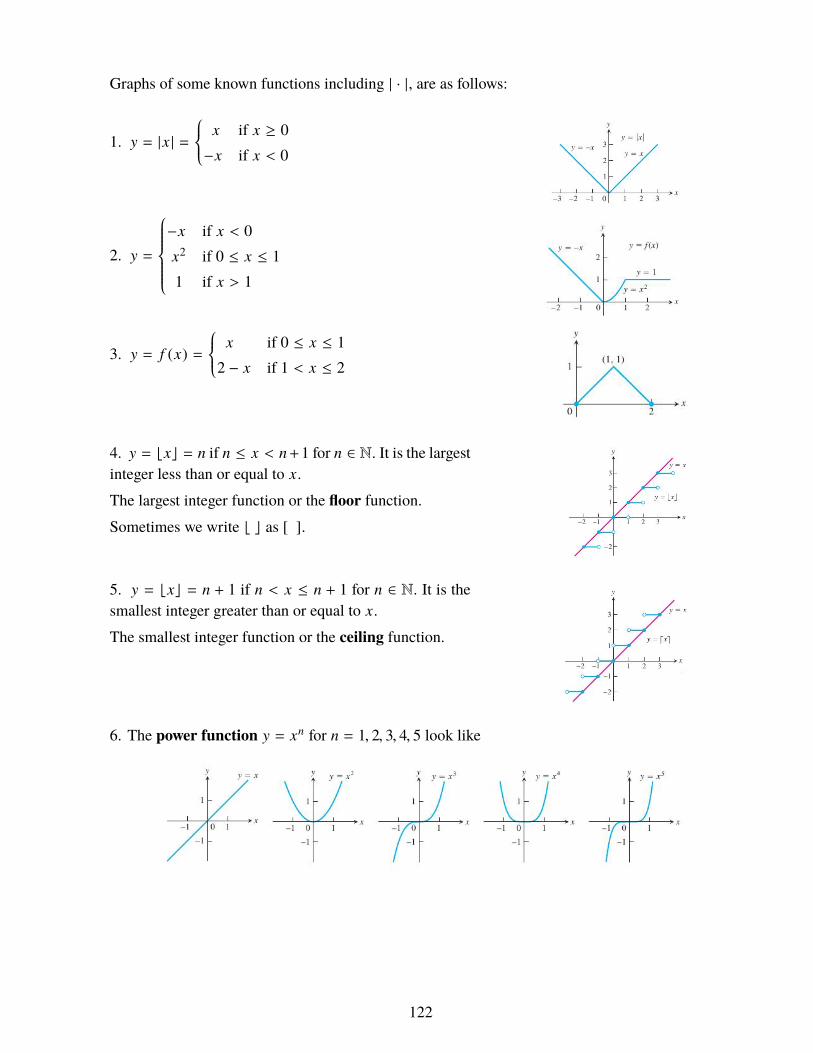
Graphs of some known functions including | · |, are as follows:

1. y = |x | =

x if x ≥ 0−x if x < 0

2. y =

−x if x < 0x2 if 0 ≤ x ≤ 11 if x > 1

3. y = f (x) =

x if 0 ≤ x ≤ 12 − x if 1 < x ≤ 2

4. y = bxc = n if n ≤ x < n+1 for n ∈ N. It is the largestinteger less than or equal to x.

The largest integer function or the floor function.Sometimes we write b c as [ ].

5. y = bxc = n + 1 if n < x ≤ n + 1 for n ∈ N. It is thesmallest integer greater than or equal to x.

The smallest integer function or the ceiling function.

6. The power function y = xn for n = 1, 2, 3, 4, 5 look like

122

7. The power function y = xn for n = −1 and n = −2 look like

8. The graphs of the power function y = xa for a = 12,

13,

32 and a = 2

3 are

9. Polynomial functions are y = f (x) = a0+ a1x+ a2x2+ · · · anxn for some n ∈ N∪ {0}. Here, thecoefficients of powers of x are some given real numbers a0, . . . , an and an , 0. The highest powern in the polynomial is called the degree of the polynomial. Graphs of some polynomial functionsare as follows:

123

10. A rational function is a ratio of two polynomials; f (x) = p(x)q(x), where p(x) and q(x) are

polynomials, may or may not be of the same degree. Graphs of some rational functions are asfollows:

11. Algebraic functions are obtained by adding subtracting, multiplying, dividing or taking rootsof polynomial functions. Rational functions are special cases of algebraic functions. Some graphsof alhebraic functions:

12. Trigonometric functions come from the ratios of sides of a right angled triangle. The anglesare measured in radian. The trigonometric functions have a period. That is, f (x + p) = f (x)happens for some p > 0. The period of f (x) is the minimum of such p. The period for sin x is 2π.

The functions cos x and sec x are even functions and all others are odd functions. Recall that f (x)is even if f (−x) = f (x) and it is odd if f (−x) = − f (x) for each x in the domain of the function.Some of the useful inequalities are

−|x | ≤ sin x ≤ |x | for all x ∈ R.

−1 ≤ sin x, cos x ≤ 1 for all x ∈ R.

0 ≤ 1 − cos x ≤ |x | for all x ∈ R.

sin x ≤ x ≤ tan x for all x ∈ (0, π/2).

In fact, if x , 0, then sin x < |x |.

Graphs of the trigonomaetric functions are as follows:

124

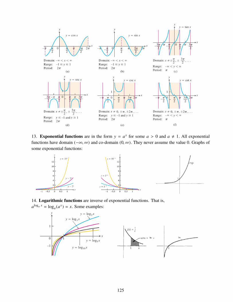
13. Exponential functions are in the form y = ax for some a > 0 and a , 1. All exponentialfunctions have domain (−∞,∞) and co-domain (0,∞). They never assume the value 0. Graphs ofsome exponential functions:

14. Logarithmic functions are inverse of exponential functions. That is,aloga x = loga (ax) = x. Some examples:

125

15. Trigonometric inverse functions:

Functions that are not algebraic are called transcendental functions. Trigonometric functions,exponential functions, logarithmic functions and inverse trigonometric functions are examples oftranscendental functions.

A.2 Concepts and FactsLet a < c < b. Let f : D → R be a function whose domain D contains the union (a, c) ∪ (c, b).Let ` ∈ R.We say that the limit of f (x) as x approaches c is ` and write it as

limx→c

f (x) = `

iff for each ε > 0, there exists a δ > 0 such that for each x ∈ (a, c) ∪ (c, b) with 0 < |x − c| < δ,

we have | f (x) − ` | < ε.

126

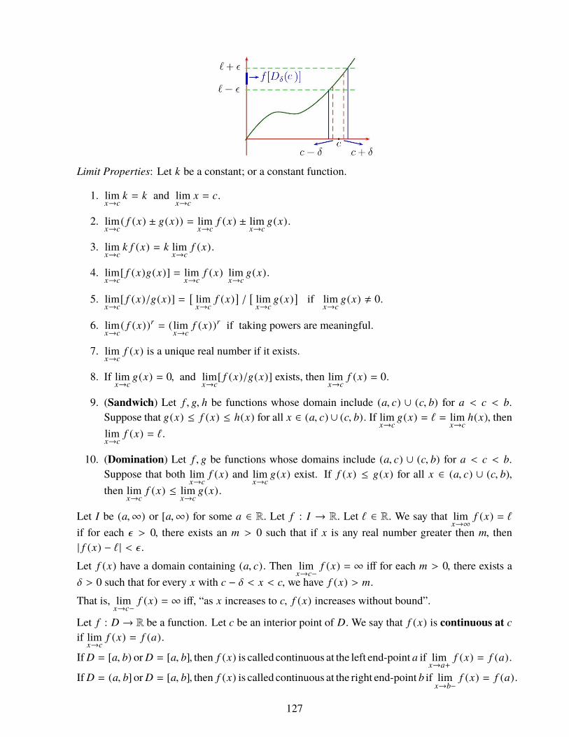
Limit Properties: Let k be a constant; or a constant function.

1. limx→c

k = k and limx→c

x = c.

2. limx→c

( f (x) ± g(x)) = limx→c

f (x) ± limx→c

g(x).

3. limx→c

k f (x) = k limx→c

f (x).

4. limx→c

[ f (x)g(x)] = limx→c

f (x) limx→c

g(x).

5. limx→c

[ f (x)/g(x)] =[

limx→c

f (x)]/[

limx→c

g(x)]

if limx→c

g(x) , 0.

6. limx→c

( f (x))r = (limx→c

f (x))r if taking powers are meaningful.

7. limx→c

f (x) is a unique real number if it exists.

8. If limx→c

g(x) = 0, and limx→c

[ f (x)/g(x)] exists, then limx→c

f (x) = 0.

9. (Sandwich) Let f , g, h be functions whose domain include (a, c) ∪ (c, b) for a < c < b.Suppose that g(x) ≤ f (x) ≤ h(x) for all x ∈ (a, c) ∪ (c, b). If lim

x→cg(x) = ` = lim

x→ch(x), then

limx→c

f (x) = `.

10. (Domination) Let f , g be functions whose domains include (a, c) ∪ (c, b) for a < c < b.Suppose that both lim

x→cf (x) and lim

x→cg(x) exist. If f (x) ≤ g(x) for all x ∈ (a, c) ∪ (c, b),

then limx→c

f (x) ≤ limx→c

g(x).

Let I be (a,∞) or [a,∞) for some a ∈ R. Let f : I → R. Let ` ∈ R. We say that limx→∞

f (x) = `if for each ε > 0, there exists an m > 0 such that if x is any real number greater then m, then| f (x) − ` | < ε.

Let f (x) have a domain containing (a, c). Then limx→c−

f (x) = ∞ iff for each m > 0, there exists aδ > 0 such that for every x with c − δ < x < c, we have f (x) > m.

That is, limx→c−

f (x) = ∞ iff, “as x increases to c, f (x) increases without bound”.

Let f : D → R be a function. Let c be an interior point of D.We say that f (x) is continuous at cif lim

x→cf (x) = f (a).

If D = [a, b) or D = [a, b], then f (x) is called continuous at the left end-point a if limx→a+

f (x) = f (a).

If D = (a, b]or D = [a, b], then f (x) is called continuous at the right end-point b if limx→b−

f (x) = f (a).

127

f (x) is called continuous if it is continuous at each point of its domain D.

The sum, multiplication by a constant, and product of continuous functions is continuous. Inaddition, the following are some properties of continuous functions:

1. Let f (x) be continuous at x = c, where the domain of f (x) includes a neighborhood of c. Iff (c) > 0, then there exists a neighborhood (c − δ, c + δ) such that f (x) > 0 for each pointx ∈ (c − δ, c + δ).

2. Let f (x) be a continuous function, whose domain contains [a, b] for a < b. Then there existα, β ∈ R such that { f (x) : x ∈ [a, b]} = [α, β].

3. (Extreme Value Theorem) Let f (x) be continuous on a closed bounded interval [a, b]. Thenthere exist numbers c, d ∈ [a, b] such that f (c) ≤ f (x) ≤ f (d) for each x ∈ [a, b].

4. (Intermediate Value Theorem) Let f (x) be continuous on a closed bounded interval [a, b].Let d be a number between f (a) and f (b). Then there exists c ∈ [a, b] such that f (c) = d.

Let f (x) be a function whose domain includes an open interval (a, b). Let c ∈ (a, b). If the limit

limh→0

f (c + h) − f (c)h

exists, we say that f (x) is differentiable at x = c; and we write the limit as f ′(c) and call it thederivative of f (x) at x = c. If f ′(c) exists for each c ∈ (a, b), then we write f ′(x) as df

dx .

Also, derivative of f defined on a closed interval [a, b] at the end-point a is taken as the left handderivative, where in the defining limit of the derivative we take h → a − . Similarly, derivative at bis taken as the limit of that ratio for h → 0 + .Let f (x) be a function defined on an interval I .We say that f (x) is increasing on I if for all s < t ∈ I, f (s) < f (t).Similarly, we say that f (x) is decreasing on I if for all s < t ∈ I, f (s) > f (t).A monotonic function on I is one which either increases on I or decreases on I .

The sum, multiplication by a constant, and product of differentiable functions is differentiable. Inaddition, the following are some properties of differentiable functions:

1. Each function differentiable at x = c is continuous at x = c.

2. Derivatives of Sum, product etc. are respectives equal to sum, product etc of derivatives.

3. (Chain Rule) dg( f (x))dx =

dg( f (x))df (x) ·

df (x)dx .

4. (Rolle’s Theorem) Suppose that f : [a, b]→ R is continuous, f (x) is differentiable on (a, b),and f (a) = f (b). Then f ′(c) = 0 for some c ∈ (a, b).

5. (Mean value Theorem) Suppose that f : [a, b] → R is continuous and f (x) is differentiableon (a, b). Then there exists c ∈ (a, b) such that f (b) − f (a) = f ′(c)(b − a).

6. Let I be an interval containing at least two points. Let f : I → R be differentiable. Iff ′(x) = 0 for each x ∈ I, iff f (x) is a constant function.

128

7. (Cauchy Mean Value Theorem) Let f (x) and g(x) be continuous on [a, b] and differentiableon (a, b). If g′(x) , 0 on (a, b), then there exists c ∈ (a, b) such that f ′(c)

g′(c) =f (b)− f (a)g(b)−g(a) .

8. (L’Hospital’s Rule) Let f (x) and g(x) be differentiable on a neighborhood of a point x = a.Suppose f (a) = g(a) = 0 but g(x) , 0, g′(x) , 0 in the deleted neighborhood of x = a. If

limx→a

f ′(x)g′(x)

exists, then limx→a

f (x)g(x)

= limx→a

f ′(x)g′(x)

.

9. Let f (x) be continuous on [a, b] and differentiable on (a, b).

(a) If f ′(x) > 0 on (a, b), then f (x) is increasing on [a, b].

(b) If f ′(x) < 0 on (a, b), then f (x) is decreasing on [a, b].

Let a function f (x) have domain D. The function f (x) has a local maximum at a point d ∈ D iff (x) ≤ f (d) for every x in some neighborhood of d contained in D. in such a case, we also saythat the point x = d is a point of local maximum of the function f (x).

Similarly, f (x) has an local minimum at b ∈ D if f (b) ≤ f (x) for every x in some neighborhoodof b contained in D. In this case, we say that the point x = b is a point of local minimum of thefunction f (x).

The points of local maximum and local minimum are commonly referred to as local extremumpoints; and the function is said to have local extrema at those points.Let f (x) have domain D. A point c ∈ D is called a critical point of f (x) if c is not an interiorpoint of D, or if f (x) is not differentiable at x = c, or if f ′(c) = 0.If f (x) has an extremum at x = c, then c is a critical point of f (x).

Test for Local Extrema:Let c be an interior point of the domain of f (x) with f ′(c) = 0.

f ′(x) changes sign from + to − at x = c iff x = c is a point of local maximum of f (x).

If f ′′(c) < 0, then x = c is a point of local maximum of f (x).

f ′(x) changes sign from − to + at x = c iff x = c is a point of local minimum of f (x).

If f ′′(c) > 0, then x = c is a point of local minimum of f (x).

Let x = c be a left end-point of the domain of f (x).

f ′(x) < 0 on the immediate right of x = c iff x = c is a point of local maximum of f (x).

f ′(x) > 0 on the immediate right of x = c iff x = c is a point of local minimum of f (x).

Let x = c be a right end-point of the domain of f (x).

f ′(x) > 0 on the immediate left of x = c iff x = c is a point of local maximum of f (x).

f ′(x) < 0 on the left of x = c iff x = c is a point of local minimum of f (x).

129

The graph of a function y = f (x) is concave up on an open interval I if f ′(x) is increasing on I .The graph of y = f (x) is concave down on an open interval I if f ′(x) is decreasing on I .A point of inflection is a point where y = f (x) has a tangent and the concavity changes.

Second derivative test for concavity:Let y = f (x) be twice differentiable on an interval I .

If f ′′(x) > 0 on I, then the graph of y = f (x) is concave up over I .

If f ′′(x) < 0 on I, then the graph of y = f (x) is concave down over I .

If f ′′(x) is positive on one side of x = c and negative on the other side, then the point(c, f (c)) on the graph of y = f (x) is a point of inflection.

Let f : [a, b]→ R. Divide [a, b] into smaller sub-intervals by choosing the break points as

a = x0 < x1 < . . . < xn = b.

The set P = {x0, x1, . . . , xn} is called a partition of [a, b].Now P divides [a, b] into n sub-intervals: [x0, x1], · · · , [xn−1, xn]. Here, the kth sub-interval is[xk−1, xk]. The area under the curve y = f (x) raised over the kth sub-interval is approximated byf (ck )(xk − xk−1) for some choice of the point ck ∈ [xk−1, xk].Write the choice points (also called sample points) as a set C = {c1, . . . , cn}.

Then the Riemann sum

S( f , P,C) =n∑

k=1f (ck )(xk − xk−1)

is an approximation to the whole area raised over [a, b] and lying between the curve y = f (x) andthe x-axis. By taking the norm of the partition as ‖P‖ = max

k(xk − xk−1), we would say that when

the norm of the partition approaches 0, the Riemann sum would approach the required area. Thus,we define the area of the region bounded by the lines x = a, x = b, y = 0, and y = f (x) as

lim‖P‖→0

n∑k=1

f (ck )(xk − xk−1)

provided that this limit exists. We define this limit (which is the mentioned area here) as the definiteintegral of f on the interval [a, b]. That is,∫ b

af (x) dx = lim

‖P‖→0

n∑k=1

f (ck )(xk − xk−1).

Let f : [a, b]→ R be a continuous function. Then∫ b

a f (x) dx exists.The definite integral has the following properties:

130

(Properties of Definite Integral)

1. Let f (x) have domain [a, b]. Let c ∈ (a, b). Then f (x) is integrable on [a, b] iff f (x) isintegrable on both [a, c] and [c, b]. In this case,∫ b

af (x)dx =

∫ c

af (x)dx +

∫ b

cf (x)dx.

2. Let f (x) and g(x) be integrable on [a, b]. Then ( f + g)(x) is integrable on [a, b] and∫ b

a( f + g)(x)dx =

∫ b

a( f (x) + g(x)) dx =

∫ b

af (x) dx +

∫ b

ag(x) dx.

3. Let f (x) be integrable on [a, b]. Let c ∈ R. Then (c f )(x) is integrable on [a.b] and∫ b

a(c f )(x) dx =

∫ b

ac f (x) dx = c

∫ b

af (x) dx.

4. Let f (x) and g(x) be integrable on [a, b]. If for each x ∈ [a, b], f (x) ≤ g(x), then∫ b

af (x) dx ≤

∫ b

ag(x) dx.

5. Let f (x) be integrable on [a, b]. If m ≤ f (x) ≤ M for all x ∈ [a, b], then

m(b − a) ≤∫ b

af (x) dx ≤ M (b − a).

6. (Average Value Theorem) Let f (x) be continuous on [a, b]. Then there exists c ∈ [a, b] suchthat

f (c) =1

b − a

∫ b

af (x) dx.

7. Let f (x) be continuous on [a, b]. If f (x) has the same sign on [a, b] and∫ b

af (x) dx = 0,

then f (x) is the zero function, i.e., f (x) = 0 for each x ∈ [a, b].

We extend the integral even when a ≮ b by the following:

If a = b, then we take∫ b

af (x) dx = 0.

If a > b, then we take∫ b

af (x) dx = −

∫ a

bf (x) dx.

Also, for any real number c; even when c is outside the interval (a, b) we have∫ b

af (x) dx =

∫ c

af (x) dx +

∫ b

cf (x) dx

In all these extensions, we assume that the definite integrals exist.The main result that shows that differentiation and integration are reverse processes is the following:

131

(Fundamental Theorem of Calculus) Let f (x) be continuous on [a, b].

1. If F (x) is an antiderivative of f (x), then∫ b

a f (x) dx = F (b) − F (a).

2. The function g(x) =∫ x

a f (t) dt is continuous on [a, b] and differentiable on (a, b).Moreover,g′(x) = d

dx

∫ xa f (t) dt = f (x).

The chain rule for differentiation is translated to integration as follows:(Substitution)

1. Let u = g(x) be a differentiable function whose range is an interval I . Let f (x) be continuouson I . Then ∫

f (g(x))g′(x) dx =∫

f (u) du.

2. Let u = g(x) be a continuously differentiable function on [a, b] whose range is an interval I .Let f (x) be continuous on I . Then∫ b

af (g(x))g′(x) dx =

∫ g(b)

g(a)f (u) du.

The rpoduct rule for differntiation gives the integration by parts formula.∫f (x)h(x) dx = f (x)

∫h(x) dx −

∫ [f ′(x)

∫h(x) dx

]dx + C.

We remember it as follows (Read F as first and S as second):

Integral of F × S = F× integral of S − integral of (derivative of F × integral of S).

The natural logarithm ln x is defined as follows:

ln x =∫ x

1

1t

dt for x > 0.

The exponential function is the inverse of the natural logarithm. That is,

exp : R→ (0,∞); y = exp(x) iff x = ln y.

Since exp(x) exp(y) = exp(x + y) and exp(0) = 1, we write

exp(x) = ex, where e = exp(1).

Then hyperbolic functions are defined by

sinh x =ex − e−x

2, cosh x =

ex + e−x

2, tanh x =

ex − e−x

ex + e−x .

sinh−1 x = ln(x +√

x2 + 1), cosh−1 x = ln(x +√

x2 − 1), tanh−1 x =12

ln(1 + x1 − x

).

132

Notice that cosh−1 has domain as x ≥ 1 and tanh−1 has domain as −1 < x < 1.Let C be a curve given parametrically by x = f (t), y = g(t), a ≤ t ≤ b. Assdume that both f (t)and g(t) are continuously differentiable.

Length of the curve = L =∫ b

a

√[ f ′(t)]2 + [g′(t)]2 dt.

If the curve is given as a function y = f (x), a ≤ x ≤ b, then take x = t and y = f (t) as itsparameterization. We then have the length as

L =∫ b

a

√1 + [ f ′(x)]2 dx =

∫ b

a

√1 + (y′)2 dx.

Notice that this formula is applicable when f ′(x) is continuous on [a, b].

We write L =∫ b

a ds with limits a and b for the variable of integration, which may be x, y or t.Here,

ds =√

[x ′(t)]2 + [y′(t)]2 dt =√

(dx)2 + (dy)2 =

√1 +

( dydx

)2dx =

√1 +

( dxdy

)2dy.

Suppose that a curve is given in polar coordinates by r = f (θ) for a continuous function f (θ),where α ≤ θ ≤ β. Then the area of the sector and the arc length of the curve are

Area =∫ β

αr2 dθ, Length =

∫ β

α

√r2 + (r′)2 dθ.

A.3 FormulasHere are some formulas for the exponential and the logarithm functions:

limt→∞

tp

at = 0 for p ∈ N and a > 1.

ln e = 1 = e0, eln x = x, ln(ex) = x, ax = ex ln a,

limx→∞

ln x = ∞, limx→0+

ln x = −∞, limx→∞

ex = ∞, limx→−∞

ex = 0,

(ln x)′ =1x, (ex)′ = ex, (ax)′ = (ln a)ax,

∫ e

1

1t

dt = 1,∫

ex dx = ex .

limh→0

ln(1 + xh)xh

= 1 for x , 0, limh→0

eh − 1h= 1, lim

h→0(1 + xh)1/h = ex,

Below are given some integrals, from which you should get the derivatives by following the simplerule that if

∫f (x) dx = g(x) + c, then g′(x) = f (x).

133

134

135

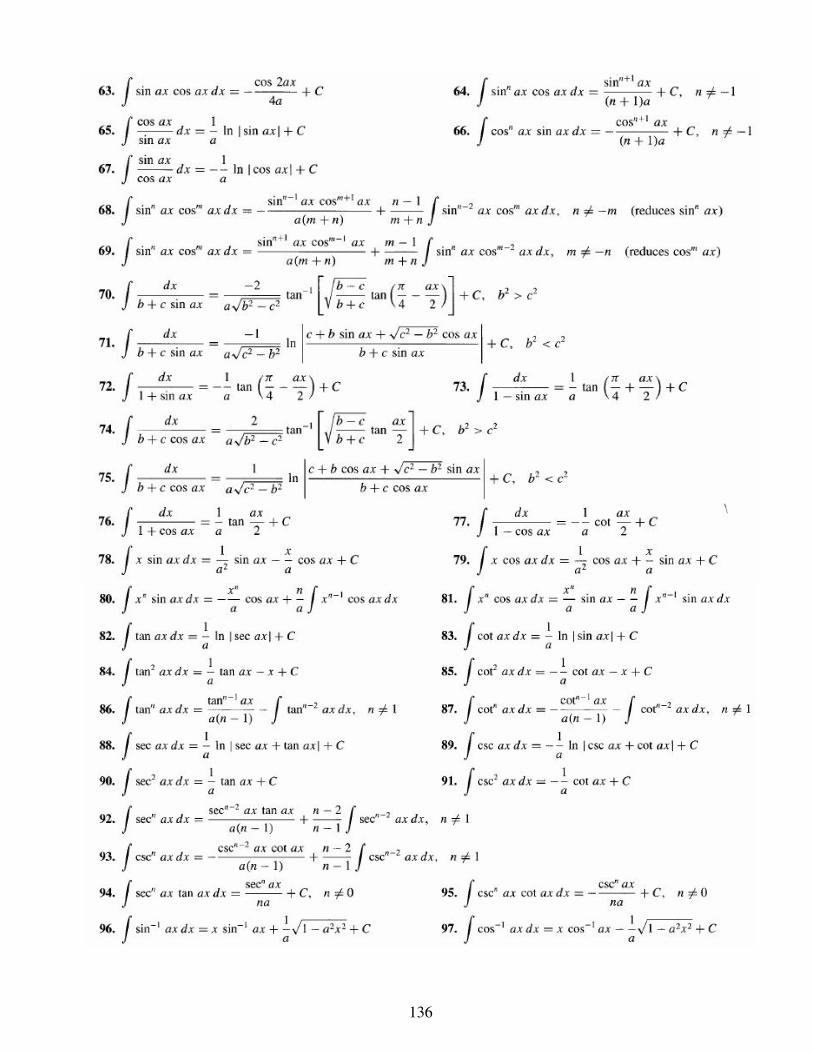
136

137

Index

absolute maximum, 29absolute maximum value, 29absolute value, 121algebraic functions, 124area of surface, 96auxiliary function, 35average value theorem, 131axis of revolution, 40

boundary point, 4bounded subset, 4

Cauchy MVT, 129ceiling function, 122closed curve, 81closed subset, 4closure, 4co-domain, 5concave down, 130concave up, 130conservative, 80continuous, 10, 127continuous on, 10contour curves, 5critical point, 29, 129curl of #»

F , 89

decreasing, 128degree of polynomial, 123differentiable, 18differentiable at a point, 128differential, 17differential form, 83directional derivative, 22disk, 4

divergence, 90, 111domain of f , 5domination limit, 127double integral, 47

error, 28even function, 124exact form, 83exponential functions, 125Extreme value theorem, 128

floor function, 122flux, 90, 104flux density, 90fundamental theorem of calculus, 132

gradient, 23gradient field, 79graph, 5Green’s theorem-1, 90Green’s theorem-2, 91

Hessian, 30homogeneous, 20

incompressible fluid, 90increasing, 128independent of path, 81integrable, 47integration by parts, 132interior point, 4intermediate value theorem, 128isolated point, 4iterated integral, 47

Jacobian, 63

138

L’Hospital’s rule, 129Laplacian, 90level curve, 6level surfaces, 6limit, 6limit of f (x), 126linear approximation, 16line integral, 74, 78line integrals, 77local extrema, 129local extremum, 29local extremum points, 129local maximum, 29, 129local maximum value, 29local minimum, 129logarithmic functions, 125

mean value theorem, 128minimum, 29monotonic, 128

norm, 46, 130normal line, 25

odd function, 124open subset, 4orientable surface, 103oriented surface, 103

partial derivative, 12partition, 46, 130period of f (x), 124point of absolute maximum, 29point of inflection, 130point of local maximum, 29, 129point of local minimum, 129polar rectangle, 51polynomial functions, 123

positive orientation, 84potential, 80power function, 122properties of definite integral, 131

range, 5rational function, 124region, 5Riemann integrable, 47Riemann sum, 46, 130Rolle’s theorem, 128

saddle point, 30sample points, 46, 130sandwich theorem, 127simple curve, 82simply connected region, 82solid of revolution, 40substitution theorem, 132surface, 5surface area, 95surface integral, 99surface integral over S, 104

tangent plane, 16, 25Taylor’s formula one variable, 26tests for concavity, 130tests for local extrema, 129total differential, 17total increment, 16, 17trigonometric functions, 124

uniform partition, 47

vector field, 78Vector forms of Green’s Theorem, 91volume of solids with holes, 42

work, 78

139