CLASSIFICATION OF SYNTHETIC APERTURE RADAR...
64
CLASSIFICATION OF SYNTHETIC APERTURE RADAR IMAGES USING PARTICLE SWARM OPTIMIZATION TECHNIQUE A THESIS SUBMITTED IN PARTIAL FULFILLMENT OF THE REQUIREMENTS FOR THE DEGREE OF Master of Technology In Electronic Systems and Communications By VEDAVRATH LAKIDE Reg. No: 207EE111 Department of Electrical Engineering National Institute of Technology Rourkela-769008 (2007-2009)
Transcript of CLASSIFICATION OF SYNTHETIC APERTURE RADAR...
CLASSIFICATION OF SYNTHETIC APERTURE RADAR IMAGES USING PARTICLE SWARM
OPTIMIZATION TECHNIQUE
A THESIS SUBMITTED IN PARTIAL FULFILLMENT
OF THE REQUIREMENTS FOR THE DEGREE OF
Master of Technology
In
Electronic Systems and Communications
By
VEDAVRATH LAKIDE
Reg. No: 207EE111
Department of Electrical Engineering
National Institute of Technology
Rourkela-769008
(2007-2009)

CLASSIFICATION OF SYNTHETIC APERTURE RADAR IMAGES USING PARTICLE SWARM
OPTIMIZATION TECHNIQUE
A THESIS SUBMITTED IN PARTIAL FULFILLMENT
OF THE REQUIREMENTS FOR THE DEGREE OF
Master of Technology
In
Electronic Systems and Communications
By
VEDAVRATH LAKIDE Reg. No: 207EE111
Under the Guidance of
Prof. DIPTI PATRA
Department of Electrical Engineering
National Institute of Technology
Rourkela-769008
(2007-2009)

National Institute Of Technology
Rourkela
CERTIFICATE
This is to certify that the thesis entitled, “Classification Of Synthetic Aperture Radar
Images Using Particle Swarm Optimization Technique” submitted by Mr.
VEDAVRATH LAKIDE in partial fulfillment of the requirements for the award of Master
of Technology Degree in Electrical Engineering with specialization in “ELECTRONIC
SYSTEMS AND COMMUNICATIONS” at the National Institute of Technology, Rourkela
is an authentic work carried out by him under my supervision and guidance.
To the best of my knowledge, the matter embodied in the thesis has not been submitted to any
other University / Institute for the award of any Degree or Diploma.
Date: Prof. Dipti Patra
Department of Electrical Engineering
National Institute of Technology
Rourkela-769008

ACKNOWLEDGEMENTS
This project is by far the most significant accomplishment in my life and it would be
impossible without people who supported me and believed in me.
I would like to extend my gratitude and my sincere thanks to my honorable, esteemed
supervisor Prof. Dipti Patra, Department of Electrical Engineering. She is not only a great
lecturer with deep vision but also most importantly a kind person. I sincerely thank for her
exemplary guidance and encouragement. Her trust and support inspired me in the most
important moments of making right decisions and I am glad to work under her supervision.
I am very much thankful to our Head of the Department, Prof. Bidyadhar Subudhi,
for providing us with best facilities in the department and his timely suggestions. I am very
much thankful to Prof. P. K. Nanda for providing valuable suggestions during my thesis
work and all my teachers Prof. J. K. Satapathy, Prof. S. Das, Prof. P. K. Sahu, Prof. K. R.
Subhashini and Prof. S. Mohanthy for providing a solid background for my studies. They
have been great sources of inspiration to me and I thank them from the bottom of my heart.
I would like to thank all my friends and especially my classmates for all the
thoughtful and mind stimulating discussions we had, which prompted us to think beyond the
obvious. I‘ve enjoyed their companionship so much during my stay at NIT, Rourkela.
I would like to thank all those who made my stay in Rourkela an unforgettable and
rewarding experience.
Last but not least I would like to thank my parents, who taught me the value of hard
work by their own example. They rendered me enormous support being apart during the
whole tenure of my stay in NIT Rourkela.
Vedavrath Lakide
CONTENTS
ABSTRACT I
LIST OF FIGURES II
LIST OF TABLES III
ABBREVIATIONS USED IV
CHAPTER 1 INTRODUCTION 1
1.1 INTRODUCTION 1
1.1.1 Synthetic Aperture RADAR (SAR) 1
1.1.2 Basic Principles of Sar 3
1.1.3 Image Processing and Analysis 4
1.1.4 Features of SAR 5
1.1.5 Applications 5
1.2 Motivation 6
1.3 Literature Review 6
1.4 Contribution of Thesis Work 7
1.5 Organization of Thesis 8
CHAPTER 2 BACKGROUND OF K-MEANS AND FUZZY C-MEANS
ALGORITHM 1
2.1 Introduction 9
2.1.1. Fuzzy Sets and Membership Function 9
2.2 Data Clustering Algorithms 10
2.3. K Means Clustering Algorithm 10
2.4. Hierarchical Clustering Algorithm 12
2.5. The Fuzzy C-Means Algorithm 13
2.5.1. FCM Optimization Model 13
2.5.2. Conditions for Optimality 14
2.5.3 Fuzzy C-Means Algorithm 15
2.5.4. Fuzzy Factor 16
2.5.5. Ideal Number of Clusters ‗c‘ 16
2.5.6. Significance of Membership Function in Cluster Analysis 16
2.6. STUDY OF FUZZY C-MEANS ALGORITHM 17
2.6.1. Analysis of FCM Model 19
2.6.2. Strengths 20
2.6.3. Weaknesses 20

CHAPTER3 SYNTHETIC APERTURE RADAR IMAGE CLASSIFICATION
USING PARTICLE SWARM OPTIMIZATION TECHNIQUE 10
3.1. Introduction 21
3.1.1. Particle Swarm Optimization Technique 21
3.2. Social behavior 23
3.2.1Co-operation 23
3.3. Rate of convergence improvements 23
3.3.1. Inertia Weight 23
3.3.2 Acceleration constants 24
3.4. Classification of SAR Image Using PSO 24
3.4.1. PSO technique steps for image classification 24
3.4.2. Conclusion 25
CHAPTER 4 CLASSIFICATION ACCURACY ASSESSMENT 21
4.1. Introduction 26
4.1.1 Accuracy Assessment 26
4.2 Confusion Matrix 26
4.2.1 Overall Accuracy 27
4.3. Kappa Coefficient 28
CHAPTER 5 SIMULATIONS AND RESULTS 27
CHAPTER 6 CONCLUSION 31
6.1 Conclusions 46
6.2 Future Work 46
REFERENCES 47
I
ABSTRACT
The prime objective of this thesis work is to devise novel methodologies for
classification of Synthetic Aperture Radar (SAR) images. Classification of SAR images has
extensive applications in national economy and military field. An analyst attempts to classify
features in an SAR image by using the elements of visual interpretation to identify
homogeneous groups of pixels that represents various features or land cover classes of
interest. The SAR images, totally different from optical images, i.e. photographs, and their
visual interpretation is not straightforward. Therefore, there is need to devise novel strategies
for classification of SAR images.
Common classification procedures can be broken down into two broad subdivisions
based on the method used such as supervised classification and unsupervised classification.
SAR image classification based on unsupervised learning usually requires optimization of
some metrics. Local optimization techniques frequently fail because functions of these
metrics with respect to transformation parameters are generally nonconvex and irregular and,
therefore, global methods are often required.
In this thesis, SAR image classification problem is considered as an optimization
problem various clustering techniques are addressed in literature for SAR image
classification. This thesis focuses on an evolutionary based stochastic optimization technique
that is Particle Swarm Optimization (PSO) technique for classification of SAR images. This
technique composes of three main processes: firstly, selecting training samples for every
region in the SAR image. Secondly, training these samples using PSO, and obtain cluster
center of every region. Finally, the classification of SAR image with respect to cluster center
is obtained. To show the effectiveness of this approach, classified SAR images are obtained
and compared with other clustering techniques such as K-means algorithm and Fuzzy C-
means algorithm (FCM). The performance of PSO is found to be superior than other
techniques in terms of classification accuracy and computational complexity. The result is
validated with various SAR images.
II
LIST OF FIGURES
Figure No. Page No.
1.1(a) A radar pulse is transmitted From the Antenna to the ground 2
1.1(b) The radar pulse is scattered by the Ground targets back to the antenna 2
1.2 Resolution Improvement along Track 3
2.1 Membership Function for FCM Algorithm 16
2.2 A 10-point data set with two clusters and two outlying points 17
2.3 Distance of the Points from centroids 19
5.1.1 Three different textures of original Reo Grande River SAR image 30
5.1.2(a) The Reo Grande River SAR Image 31
5.1.2(b) The PSO classified Image 31
5.1.2(c) The FCM classified Image 31
5.1.2(d) The K-means classified Image 31
5.1.3(a) PSO classified Image pdf with cluster centers 32
5.1.3(b) FCM classified Image pdf with cluster centers 33
5.1.3(c) K-means classified Image pdf with cluster centers 33
5.2.1. Three different textures of original RADARSAT-1 SAR image 35
5.2.2(a) RADARSAT-1 SAR image 36
5.2.2(b) The PSO classified Image 36
5.2.2(c) The FCM classified Image 36
5.2.2(d) The K-means classified Image 36
5.2.3(a) PSO classified Image pdf with cluster centers 37
5.2.3(b) FCM classified Image pdf with cluster centers 38
5.2.3(c) K-means classified Image pdf with cluster centers 38
5.3.1 Three different textures of original L-band San Francisco SAR image 40
5.3.2(a) San Francisco SAR image 41
5.3.2(b) The PSO classified Image 41
5.3.2(c) The FCM classified Image 41
5.3.2(d) The K-means classified Image 41
5.3.3(a) PSO classified Image pdf with cluster centers 42
5.3.3(b) FCM classified Image pdf with cluster centers 42
5.3.3(c) K-means classified Image pdf with cluster centers 43
III
LIST OF TABLES
Table No. Page No.
2.1 Membership values of the data 18
4.1 Confusion matrix 27
4.2 Interpretation of K-values 29
5.1.4(a) Confusion matrix 34
5.1.4(b) Accuracy Assessment 35
5.2.4(a) Confusion matrix 39
5.2.4(b) Accuracy Assessment 40
5.3.4(a) Confusion matrix 44
5.3.4(b) Accuracy Assessment 45

IV
ABBREVIATIONS USED
SAR Synthetic Aperture Radar
FCM Fuzzy c-means algorithm
ML Maximum Likelihood
NN Neural Networks
RAR Real Aperture Radar
PSO Particle Swarm Optimization

CHAPTER 1
INTRODUCTION
1
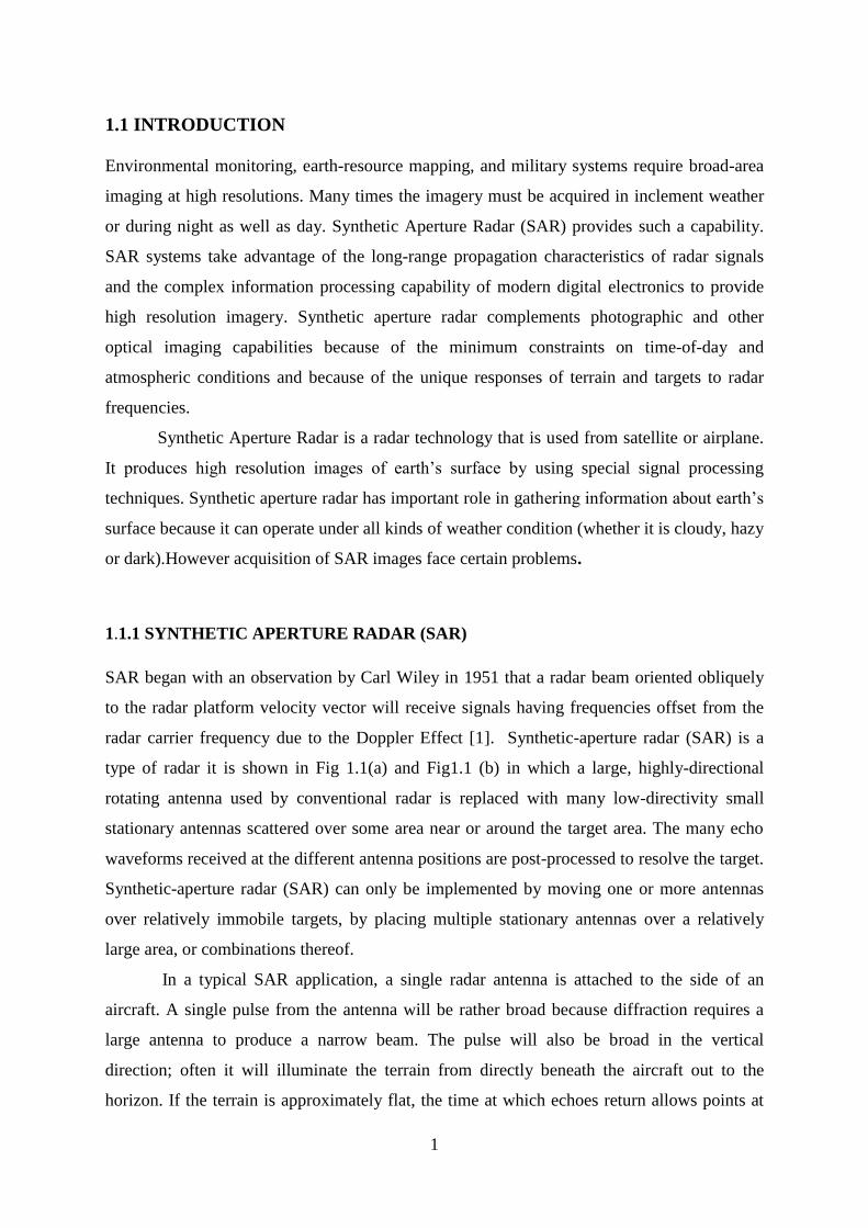
1.1 INTRODUCTION
Environmental monitoring, earth-resource mapping, and military systems require broad-area
imaging at high resolutions. Many times the imagery must be acquired in inclement weather
or during night as well as day. Synthetic Aperture Radar (SAR) provides such a capability.
SAR systems take advantage of the long-range propagation characteristics of radar signals
and the complex information processing capability of modern digital electronics to provide
high resolution imagery. Synthetic aperture radar complements photographic and other
optical imaging capabilities because of the minimum constraints on time-of-day and
atmospheric conditions and because of the unique responses of terrain and targets to radar
frequencies.
Synthetic Aperture Radar is a radar technology that is used from satellite or airplane.
It produces high resolution images of earth‘s surface by using special signal processing
techniques. Synthetic aperture radar has important role in gathering information about earth‘s
surface because it can operate under all kinds of weather condition (whether it is cloudy, hazy
or dark).However acquisition of SAR images face certain problems.
1.1.1 SYNTHETIC APERTURE RADAR (SAR)
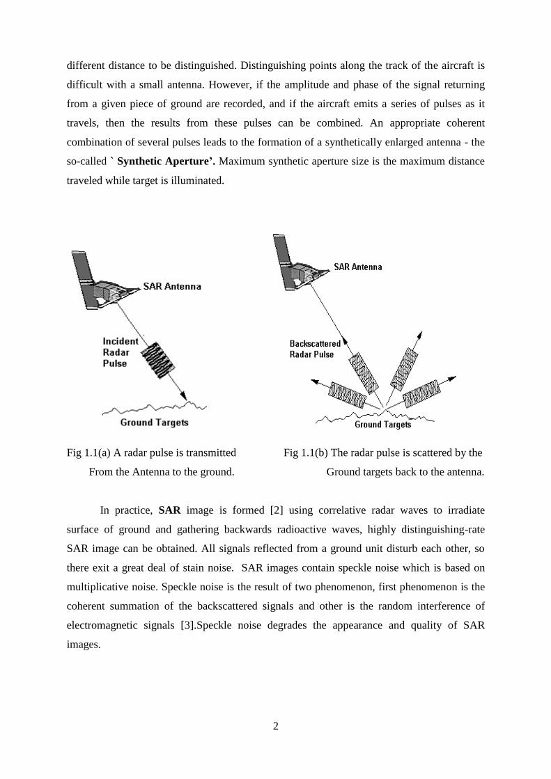
SAR began with an observation by Carl Wiley in 1951 that a radar beam oriented obliquely
to the radar platform velocity vector will receive signals having frequencies offset from the
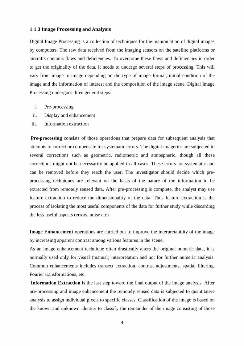
radar carrier frequency due to the Doppler Effect [1]. Synthetic-aperture radar (SAR) is a
type of radar it is shown in Fig 1.1(a) and Fig1.1 (b) in which a large, highly-directional
rotating antenna used by conventional radar is replaced with many low-directivity small
stationary antennas scattered over some area near or around the target area. The many echo
waveforms received at the different antenna positions are post-processed to resolve the target.
Synthetic-aperture radar (SAR) can only be implemented by moving one or more antennas
over relatively immobile targets, by placing multiple stationary antennas over a relatively
large area, or combinations thereof.
In a typical SAR application, a single radar antenna is attached to the side of an
aircraft. A single pulse from the antenna will be rather broad because diffraction requires a
large antenna to produce a narrow beam. The pulse will also be broad in the vertical
direction; often it will illuminate the terrain from directly beneath the aircraft out to the
horizon. If the terrain is approximately flat, the time at which echoes return allows points at
2
different distance to be distinguished. Distinguishing points along the track of the aircraft is
difficult with a small antenna. However, if the amplitude and phase of the signal returning
from a given piece of ground are recorded, and if the aircraft emits a series of pulses as it
travels, then the results from these pulses can be combined. An appropriate coherent
combination of several pulses leads to the formation of a synthetically enlarged antenna - the
so-called ` Synthetic Aperture‟. Maximum synthetic aperture size is the maximum distance
traveled while target is illuminated.
Fig 1.1(a) A radar pulse is transmitted Fig 1.1(b) The radar pulse is scattered by the
From the Antenna to the ground. Ground targets back to the antenna.
In practice, SAR image is formed [2] using correlative radar waves to irradiate
surface of ground and gathering backwards radioactive waves, highly distinguishing-rate
SAR image can be obtained. All signals reflected from a ground unit disturb each other, so
there exit a great deal of stain noise. SAR images contain speckle noise which is based on
multiplicative noise. Speckle noise is the result of two phenomenon, first phenomenon is the
coherent summation of the backscattered signals and other is the random interference of
electromagnetic signals [3].Speckle noise degrades the appearance and quality of SAR
images.
3
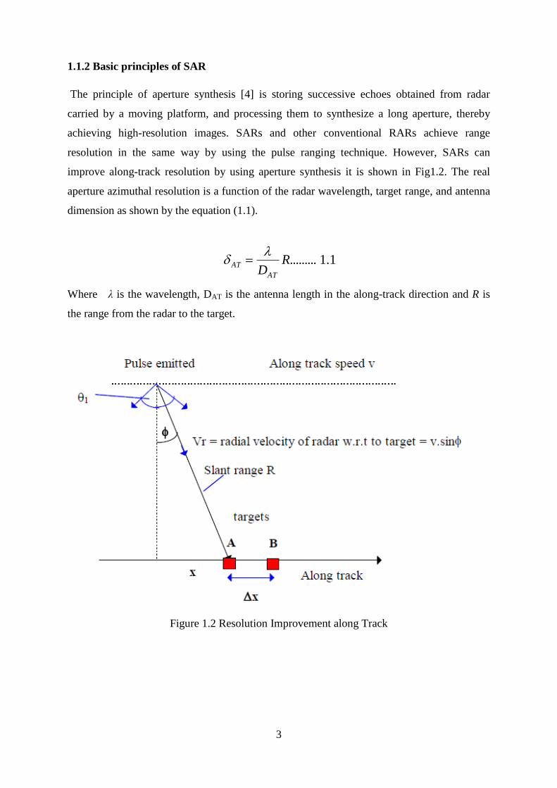
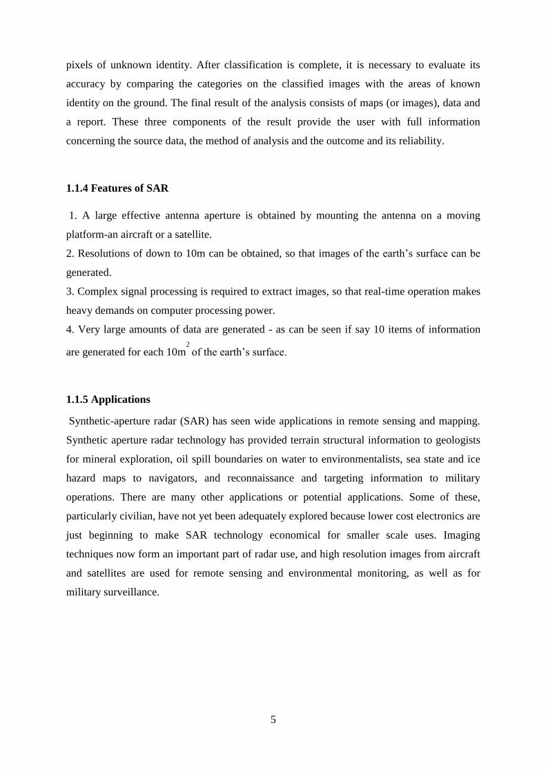
1.1.2 Basic principles of SAR
The principle of aperture synthesis [4] is storing successive echoes obtained from radar
carried by a moving platform, and processing them to synthesize a long aperture, thereby
achieving high-resolution images. SARs and other conventional RARs achieve range
resolution in the same way by using the pulse ranging technique. However, SARs can
improve along-track resolution by using aperture synthesis it is shown in Fig1.2. The real
aperture azimuthal resolution is a function of the radar wavelength, target range, and antenna
dimension as shown by the equation (1.1).
1.1.........RDAT
AT
Where λ is the wavelength, DAT is the antenna length in the along-track direction and R is
the range from the radar to the target.
Figure 1.2 Resolution Improvement along Track
4
1.1.3 Image Processing and Analysis
Digital Image Processing is a collection of techniques for the manipulation of digital images
by computers. The raw data received from the imaging sensors on the satellite platforms or
aircrafts contains flaws and deficiencies. To overcome these flaws and deficiencies in order
to get the originality of the data, it needs to undergo several steps of processing. This will
vary from image to image depending on the type of image format, initial condition of the
image and the information of interest and the composition of the image scene. Digital Image
Processing undergoes three general steps:
i. Pre-processing
ii. Display and enhancement
iii. Information extraction
Pre-processing consists of those operations that prepare data for subsequent analysis that
attempts to correct or compensate for systematic errors. The digital imageries are subjected to
several corrections such as geometric, radiometric and atmospheric, though all these
corrections might not be necessarily be applied in all cases. These errors are systematic and
can be removed before they reach the user. The investigator should decide which pre-
processing techniques are relevant on the basis of the nature of the information to be
extracted from remotely sensed data. After pre-processing is complete, the analyst may use
feature extraction to reduce the dimensionality of the data. Thus feature extraction is the
process of isolating the most useful components of the data for further study while discarding
the less useful aspects (errors, noise etc).
Image Enhancement operations are carried out to improve the interpretability of the image
by increasing apparent contrast among various features in the scene.
As an image enhancement technique often drastically alters the original numeric data, it is
normally used only for visual (manual) interpretation and not for further numeric analysis.
Common enhancements includes transect extraction, contrast adjustments, spatial filtering,
Fourier transformations, etc.
Information Extraction is the last step toward the final output of the image analysis. After
pre-processing and image enhancement the remotely sensed data is subjected to quantitative
analysis to assign individual pixels to specific classes. Classification of the image is based on
the known and unknown identity to classify the remainder of the image consisting of those
5
pixels of unknown identity. After classification is complete, it is necessary to evaluate its
accuracy by comparing the categories on the classified images with the areas of known
identity on the ground. The final result of the analysis consists of maps (or images), data and
a report. These three components of the result provide the user with full information
concerning the source data, the method of analysis and the outcome and its reliability.
1.1.4 Features of SAR
1. A large effective antenna aperture is obtained by mounting the antenna on a moving
platform-an aircraft or a satellite.
2. Resolutions of down to 10m can be obtained, so that images of the earth‘s surface can be
generated.
3. Complex signal processing is required to extract images, so that real-time operation makes
heavy demands on computer processing power.
4. Very large amounts of data are generated - as can be seen if say 10 items of information
are generated for each 10m2
of the earth‘s surface.
1.1.5 Applications
Synthetic-aperture radar (SAR) has seen wide applications in remote sensing and mapping.
Synthetic aperture radar technology has provided terrain structural information to geologists
for mineral exploration, oil spill boundaries on water to environmentalists, sea state and ice
hazard maps to navigators, and reconnaissance and targeting information to military
operations. There are many other applications or potential applications. Some of these,
particularly civilian, have not yet been adequately explored because lower cost electronics are
just beginning to make SAR technology economical for smaller scale uses. Imaging
techniques now form an important part of radar use, and high resolution images from aircraft
and satellites are used for remote sensing and environmental monitoring, as well as for
military surveillance.
6
1.2 MOTIVATION
Synthetic Aperture Radar (SAR) image classification is becoming increasingly important in
military or scientific research. SAR image processing is commonly recognized as a hard task
because of high dynamics and multiplicative noise takes place, which prevent the use of
classical image processing tools. Classification methods based on thresholding of gray levels
are generally inefficient when applied to speckled images, due to the high degree of overlap
between the distributions of the different classes. Speckle is caused by the constructive and
destructive interference between waves returned from elementary scatterers within each
resolution cell. It is generally modeled as a multiplicative random noise [4], [3].
The model based approaches are used to classify the SAR images are 1.supervised
approach, 2.unsupervised approach. In supervised frame work, the associated model
parameters are assumed to be known apriori. In unsupervised frame work the parameters
assumed to be unknown. The motivation of this dissertation is to develop a classification
algorithm for clustering which can be used to classify the SAR images and improving overall
accuracy. To show the improvement of classification accuracy the PSO classified results are
compared with standard K-means algorithm and FCM algorithm. The advantage of PSO
algorithm is initial conditions are not required and it performs a globalized searching for
solutions whereas most other partitional clustering procedures perform a localized searching.
1.3 LITERATURE REVIEW
Both visual interpretation and automatic analysis of data from imaging radars are complicated
by a fading effect called speckle, which manifests itself as a strong granularity in detected
images (amplitude or intensity). For example, simple classification methods based on
thresholding of gray levels are generally inefficient when applied to speckled images, due to
the high degree of overlap between the distributions of the different classes. Speckle is
caused by the constructive and destructive interference between waves returned from
elementary scatterers within each resolution cell. It is generally modeled as a multiplicative
random noise [4], [3]. Compared with optical image, SAR image has more legible outline,
better contrast and more plentiful texture information [2]. The objects of different shape and
physical feature take on different texture character, which is a critical technique of identifying
objects by radar. At present, there are many approaches to image classification, but there is
not an approach to suit all kinds of images. During the past years, different methods were
employed for classification of synthetic aperture radar (SAR) data [5-6], based on the
7
Maximum Likelihood (ML) [5], artificial Neural Networks (NN) [7], fuzzy methods [8, 9] or
other approaches [6-9]. The NN classifier depends only on the training data and the
discrimination power of the features. Fukuda and Hirosawa [10] applied wavelet-based
texture feature sets for classification of multi frequency polarimetric SAR images. The
Classification accuracy depends on quality of features and the employed classification
algorithm.
For a high resolution SAR image classification, there is a strong need for statistical
models of scattering to take into account multiplicative noise and high dynamics. For
instance, the classification process needs to be based on the use of statistics. Clutter in SAR
images becomes non-Gaussian when the resolution is high or when the area is man-made.
Many models have been proposed to fit with non-Gaussian scattering statistics (Weibull, Log
normal, Nakagami Rice, etc.), but none of them is flexible enough to model all kinds of
surfaces in our context [11].
For SAR image classification problem many fuzzy models have been proposed,
Fuzzy c-means clustering (FCM) algorithm [12] is widely applied in various areas such as
image processing and pattern recognition. Co-occurrence matrix and entropy calculations are
used to extract transition region for an image. This transition region approach [12] is used to
classify the SAR images.
1.4 CONTRIBUTION OF THESIS WORK
The contribution of this thesis can be summarized as follows. The thesis presents a different
approach, to solve the classification problem of SAR images. SAR image classification based
on unsupervised learning usually requires optimization of some metrics. Local optimization
techniques frequently fail because functions of these metrics with respect to transformation
parameters are generally nonconvex and irregular and, therefore, global methods are often
required. The traditional clustering methods are very sensitive to the initial value and the
number of clusters. The accurate initial value and number of clusters are important
parameters to get the accurate result. The traditional algorithm of FCM applies directly SAR
image to get the ideal result difficultly. So a novel algorithm, particle swarm optimization is
used for SAR image classification. To show the effectiveness of this approach, simulation
results of classified SAR images are considered and compared with K means algorithm
According to the overall accuracy, PSO has high classification precision and can be used in
SAR images classification efficiently.
8
1.5 ORGANIZATION OF THESIS
The thesis is organized into the following chapters
Chapter 1 (Introduction): deals with the formal description of the SAR image
formation, basics of SAR image processing and analysis and problem of SAR image
classification and the related research work already carried out in this direction. The
addressed problem is also included here.
Chapter 2 (Background of K-means and Fuzzy C-Means Algorithm): introduces the
basic definitions and concepts of fuzzy data sets and Fuzzy c-means clustering technique that
will be needed in the further chapters. It also includes the fuzzy c-means algorithm with its
examples, strengths and weakness.
Chapter 3 (Synthetic aperture radar Image classification using particle swarm
optimization technique): This chapter mainly focuses on the Particle Swarm Optimization
Technique, classification of Synthetic Aperture Radar images using Particle Swarm
Optimization and PSO algorithm steps for image classification.
Chapter 4 (Classification accuracy assessment): In this chapter accuracy assessment
procedure is described.
Chapter 5 (Simulations and Results): covers discussions on the simulation results of
SAR images.
Chapter 6 (Conclusion): includes the conclusion and the discussion for future
research.

CHAPTER2
BACKGROUND OF K-MEANS AND FUZZY C-MEANS ALGORITHM
9
2.1 INTRODUCTION
In this Chapter, the basic K-means algorithm and Fuzzy C-means (FCM) algorithms are
described. Both K-means and Fuzzy c-means algorithms are clustering algorithms.
Clustering can be considered as the most important unsupervised learning problem. So, as
every other problem of this kind, it deals with finding a structure in a collection of unlabeled
data.
A classical set is a set that has a crisp boundary. For example, a classical set X of real
numbers greater than 6 is expressed as
A= {x│x > 6}
In this set of real numbers there is a clear unambiguous boundary 6 such that if x is
greater than this number. In this case x either belongs to this set ‘A’ or it does not belong to
this set. These types of sets are called Classical Sets and the elements in this set are a part of
the set or they are not a part of the set. Classical sets are an important tool in mathematics and
computer science but they do not reflect the nature of human concepts and thought.
In contrast to a classical set, a fuzzy set is a set without crisp boundaries. That is, the
process of an element ―belongs to a set‖ to ―does not belong to a set‖ is gradual. This
transition is decided by the membership function of a fuzzy dataset. Real life problems have
data which most of the time has a degree of ―trueness‖ or ―falseness‖ that is the data cannot
be expressed in terms of classical set. A good example of this is; the same set A is a set of tall
basketball players. According to the classical set logic a player 6.01 ft tall is considered to be
tall whereas a player 5.99 ft tall is considered to be short.
2.1.1. Fuzzy Sets and Membership Function
Membership functions give fuzzy sets the flexibility in modeling commonly used linguistic
terms such as ―the water is hot‖ or ―the temperature is high.‖ Zadeh (1965) points out that,
this imprecise data set information plays an important role in human approach to problem
solving. It is important to note that fuzziness in a dataset comes does not come from the
randomness of the elements of the set, but from the uncertain and imprecise nature of the
abstract thoughts and concepts.
If X is a collection of objects denoted by x, then a fuzzy set ‘A’ in ‘X’ is defined as a set of
ordered pairs
A= {(x, μ A (x)) │ x X},

Where μ A (x) is called the membership function (MF) for the fuzzy set A. The membership
function maps each element of X to a membership grade between 0 and 1. If the value of the
membership function is restricted to either 0 or 1, then A is reduced to a classical set and μ A
(x) is the characteristic function of A. Usually X is referred to as the universe of discourse and
may consist of discrete objects or continuous space.
2.2 DATA CLUSTERING ALGORITHMS
A loose definition of clustering could be ―the process of organizing objects into groups whose
members are similar in some way‖. A cluster is therefore a collection of objects which are
―similar‖ between them and are ―dissimilar‖ to the objects belonging to other clusters.
Clustering of numerical data forms the basis of various classification and system modeling
algorithms. The purpose of clustering is to identify natural groupings of data from a large
data set to produce a concise representation of a system's behavior. Clustering algorithms are
not only used to organize and categorize data, but are helpful in data compression and model
construction.
The clustering algorithms can be categorized into two groups: hierarchical and
Partitional [13], [14]. In hierarchical clustering, the output is ―a tree showing a sequence of
clustering with each clustering being a partition of the data set‖. The partitional clustering
algorithms partition the data set into a specified number of clusters. These algorithms try to
minimize certain criteria (e.g. a square error function); therefore, they can be treated as an
optimization problem.
2.3. K MEANS CLUSTERING ALGORITHM
The K-means clustering, also known as C-means clustering, has been applied to variety of
areas, including image and speech data compression. The k-means clustering was invented in
1956. This technique is based on randomly choosing k initial cluster centers, or means. These
initial cluster centers are updated in such a way that after a number of cycles they represent
the clusters in the data as much as possible. The K-means algorithm starts with K- cluster
centers or centriodes. Cluster centriodes can be initialized to random values or can be derived
from a priori information. Each data point then assigned to the closest cluster (i.e. closest
centroide). Finally, the centriodes are recalculated according to the associated data. This
process is repeated until convergence.
11
K-means clustering groups‘ data vectors into a predefined number of clusters, based
on Euclidean distance as similarity measure. Data vectors within a cluster have small
Euclidean distances from one another, and are associated with one centroide vector, which
represents the "midpoint" of that cluster. The centroide vector is the mean of the data vectors
that belong to the corresponding cluster.
1. The algorithm starts out with initializing Ci this is achieved by randomly Selecting C
points from among all the data points.
2. The algorithm starts out with initializing Ci this is achieved by randomly Selecting C
points from among all the data points.
3. Determine the membership matrix U, where the element uij is 1 if the jth data point xj
belongs to the group 1 and 0 otherwise.
4. Compute the cost function by the equation given below. Stop if the value of cost
function is below a certain threshold value.
5. Assign each data point to the cluster closest centroide.
6. Update the clusters center centers Ci by re calculating the clusters centriodes as mean
of all data points within the each cluster and determine the new U matrix.
Parameters and options for the k-means algorithm: Number of classes,
Initialization, Distance measure, Termination.
Drawbacks of the k-means algorithm are that the number of clusters is fixed; once k is
chosen it always remains k cluster centers. The K-means algorithm circumvents the problem
by removing the redundant clusters. Whenever a cluster centre is not assigned enough
samples, it may be removed. In this way one is left with a more or less optimal number of
clusters. The problem of choosing the initial number of clusters still remains unsolved, but by
taking k large enough this will usually not be a problem. For the analysis of large datasets—
the method is computationally inefficient. Each step of the procedure requires calculation of
the distance between every possible pair of data points and comparison of all the distances. It
is a greedy algorithm that depends on the initial conditions, which may cause the algorithm to
converge to suboptimal solutions.
12
2.4. HIERARCHICAL CLUSTERING ALGORITHM
In hierarchical clustering the data is not partitioned into a particular cluster in a single step.
Instead, a series of partitions takes place that run from a single cluster containing all objects
to N clusters each containing a single object. Hierarchical clustering is further classified as
agglomerative method, which proceed by series of fusions of the N objects into groups, and
divisive method, which separate N objects successively into finer groupings. Hierarchical
clustering may be represented by a two-dimensional diagram known as dendrogram, which
illustrates the fusion or divisions made at each successive stage of analysis. Given a set of N
items to be clustered, and an NxN distance matrix, the basic process of Johnson's (1967)
hierarchical clustering is briefly explained below.
1. The algorithm starts by assigning each item to its own cluster, such that for N items,
we have N clusters, each containing just one item. Let the distances between the
clusters equal the distances between the items they contain.
2. Find the closest (most similar) pair of clusters and merge them into a single cluster, so
that we have one less cluster.
3. Compute distances between the new cluster and each of the old clusters.
4. Repeat steps 2 and 3 until all items are clustered into a single cluster of size N.
Step 3 can be done in different ways, which is what distinguishes single-link from
complete-link and average-link clustering. In single-link, clustering (also called the
connectedness or minimum method); we consider the distance between one cluster and
another cluster to be equal to the shortest distance from any member of one cluster to any
member of the other cluster. If the data consist of similarities, we consider the similarity
between one cluster and another cluster to be equal to the largest similarity from any member
of one cluster to any member of the other cluster. In complete-link, clustering (also called the
diameter or maximum method); we consider the distance between one cluster and another
cluster to be equal to the longest distance from any member of one cluster to any member of
the other cluster. In average-link clustering, we consider the distance between one cluster and
another cluster to be equal to the average distance from any member of one cluster to any
member of the other cluster.
Today, Synthetic Aperture Radar (SAR) image classification is becoming increasingly
important in military or scientific research. The large amount of data involved necessitates
the identification or segmentation of the objects of interest before further analysis can be
made. The result of this segmentation or classification process is the labeling or grouping of
pixels into meaningful regions or classes. There is a very strong intuitive similarity between
13
clustering and segmentation; both processes share the goal of finding accurate classification
of their input. Fuzzy clustering, therefore, has been used for image segmentation for the past
twenty years. FCM‘s objective function has been generalized and extended as well as
changed in several ways. For this reason, FCM is sometimes described as a model for fuzzy
clustering. Our aim in this Chapter will be to define and describe the FCM model. We also
highlight the strengths and shortcomings that this algorithm. In the next Chapter, we propose
our particle swarm optimization technique for SAR image classification.
2.5. THE FUZZY C-MEANS ALGORITHM
Fuzzy C-means clustering (FCM) algorithm, also known as fuzzy Isodata, is a data clustering
algorithm in which each data point belongs to a cluster to a degree specified by a membership
grade. Bezdek proposed this algorithm in 1973 as an improvement to K means algorithm
also known as the hard C-means algorithm. Hard k-means algorithm executes a sharp
classification, in which each object is either assigned to a class or not. The application of
fuzzy clustering to the dataset function allows the class membership to have several classes at
the same time but with different degrees of membership function ranging from 0 to 1. Fuzzy
c-means (FCM) is a method of clustering which allows one piece of data to belong to two or
more clusters. It is based on minimization of the objective function
2.5.1. FCM Optimization Model
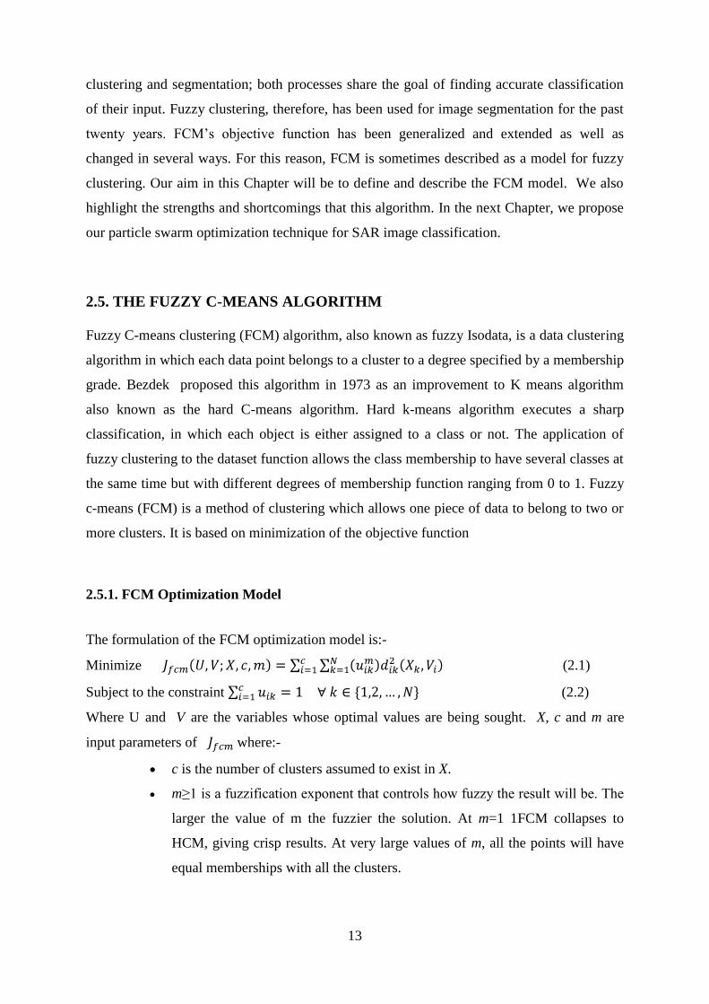
The formulation of the FCM optimization model is:-
Minimize (2.1)
Subject to the constraint (2.2)
Where U Pand V Uare the variables whose optimal values are being sought. X, c and m are
input parameters of where:-
c is the number of clusters assumed to exist in X.
m≥1 is a fuzzification exponent that controls how fuzzy the result will be. The
larger the value of m the fuzzier the solution. At m=1 1FCM collapses to
HCM, giving crisp results. At very large values of m, all the points will have
equal memberships with all the clusters.
14
uik describes the degree of membership of feature vector xkwith the cluster
represented by . is the c x N Fuzzy partition matrix satisfying the
constraint stated in (2.2).
N is the total number of feature vectors.
is the distance between feature vector xkand prototype The original
formulation of FCM uses point prototypes and an inner-product induced-norm
metric for given by
(2.3)
A : is any positive definite matrix which in the case of Euclidean distance is the
identity matrix.
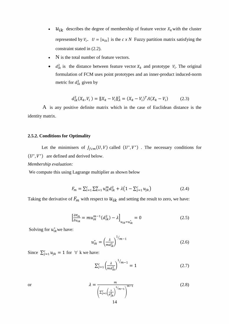
2.5.2. Conditions for Optimality
Let the minimisers of J called . The necessary conditions for
( Pare defined and derived below.
Membership evaluation:
We compute this using Lagrange multiplier as shown below
(2.4)
Taking the derivative of with respect to and setting the result to zero, we have:
(2.5)
Solving for we have:
(2.6)
Since for k we have:
(2.7)
or (2.8)

15
Substituting the above equation into (2.6), the zero-gradient condition for the membership
estimator can be rewritten as:
(2.9)
Cluster prototype updating:
Taking the derivative of with respect to and setting the result to zero, we have:
(2.10)
(2.11)
(2.12)
Solving for , we have:
(2.13)
The FCM algorithm is a sequence of iterations through the equations (2.9), (2.13), which are
referred to as the update equations. When the iteration converges, a fuzzy c-partition matrix
and the pattern prototypes are obtained.
2.5.3 Fuzzy C-Means Algorithm
1.fix c, 2≤c≤N,m,1≤m≤∞ initialize The class prototypes V
2. Compute the partition matrix using (2.9).
3. Update fuzzy cluster centers V using (2.13).
4. Compare the change in the cluster centers values using a appropriate norm; if the change is
Small, stop. Else return to 2.
16
2.5.4. Fuzzy Factor
The fuzzy factor ‗m‘ was introduced by Bezdek and is also known as ‗fuzzifier‘ As the value
of m approaches 1 the clusters formed tend to be hard and as the value of m tends to infinity
the obtained clusters tend to go in a the fuzziest state. There is no theoretical justification on
the value of ‗m‘ but is usually set to 2 and in a more generalized form tends to be between 1.5
and 3 (Zimmermann, 1990).
2.5.5. Ideal Number of Clusters „c‟
From the research on decision of ideal number of clusters for the FCM algorithm, they find
out that there is nothing called as an ideal number of clusters (Zimmermann, 1990). The
number of clusters for a certain type of data will vary based on the data partition desired. The
number of clusters can vary between 2 to infinity.
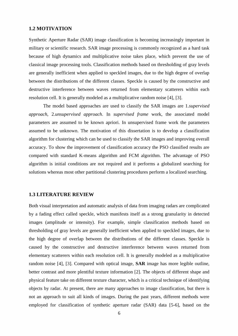
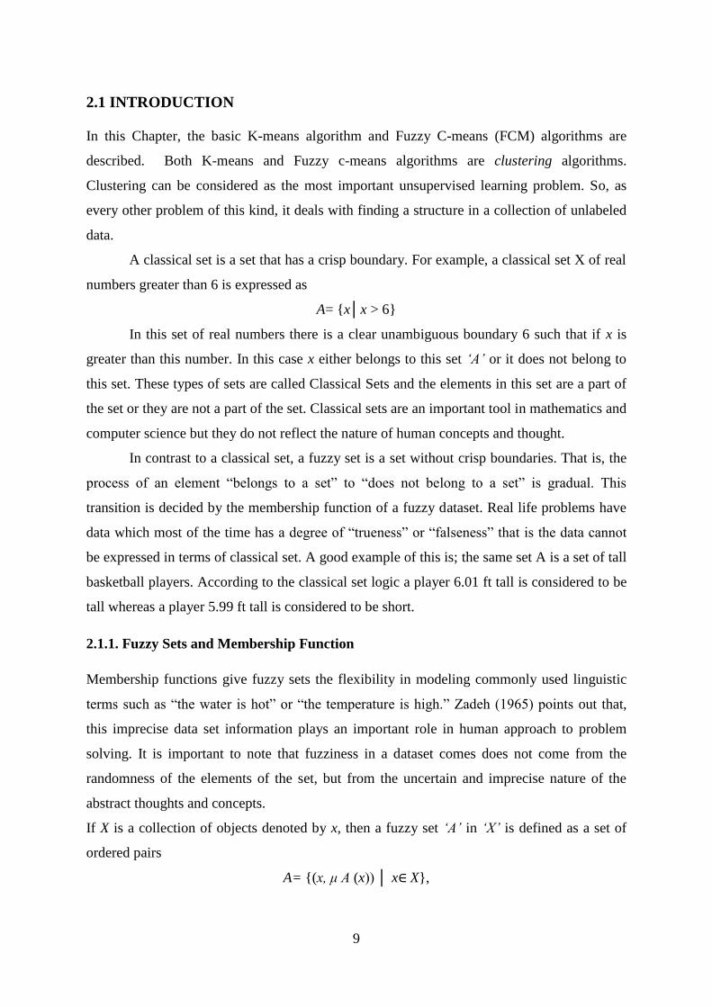
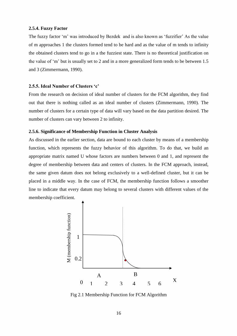
2.5.6. Significance of Membership Function in Cluster Analysis
As discussed in the earlier section, data are bound to each cluster by means of a membership
function, which represents the fuzzy behavior of this algorithm. To do that, we build an
appropriate matrix named U whose factors are numbers between 0 and 1, and represent the
degree of membership between data and centers of clusters. In the FCM approach, instead,
the same given datum does not belong exclusively to a well-defined cluster, but it can be
placed in a middle way. In the case of FCM, the membership function follows a smoother
line to indicate that every datum may belong to several clusters with different values of the
membership coefficient.
0.2
Fig 2.1 Membership Function for FCM Algorithm
A B
1 2 3 4 5 6
……………………
X
1
0
M (
mem
ber
ship
funct
ion
)
17
In Fig 2.1 (George and Yuan, 1995), the datum shown as a red marked spot belongs more to
the cluster B rather than the cluster A. The value 0.2 of membership function indicates the
degree of membership to A for such datum. Now, instead of using a graphical representation,
we introduce a matrix whose factors are the ones taken from the membership functions.
The number of rows and columns depends on how many data and clusters we are
considering. Here C (columns) is the total number of clusters and N (rows) is the total data
points.
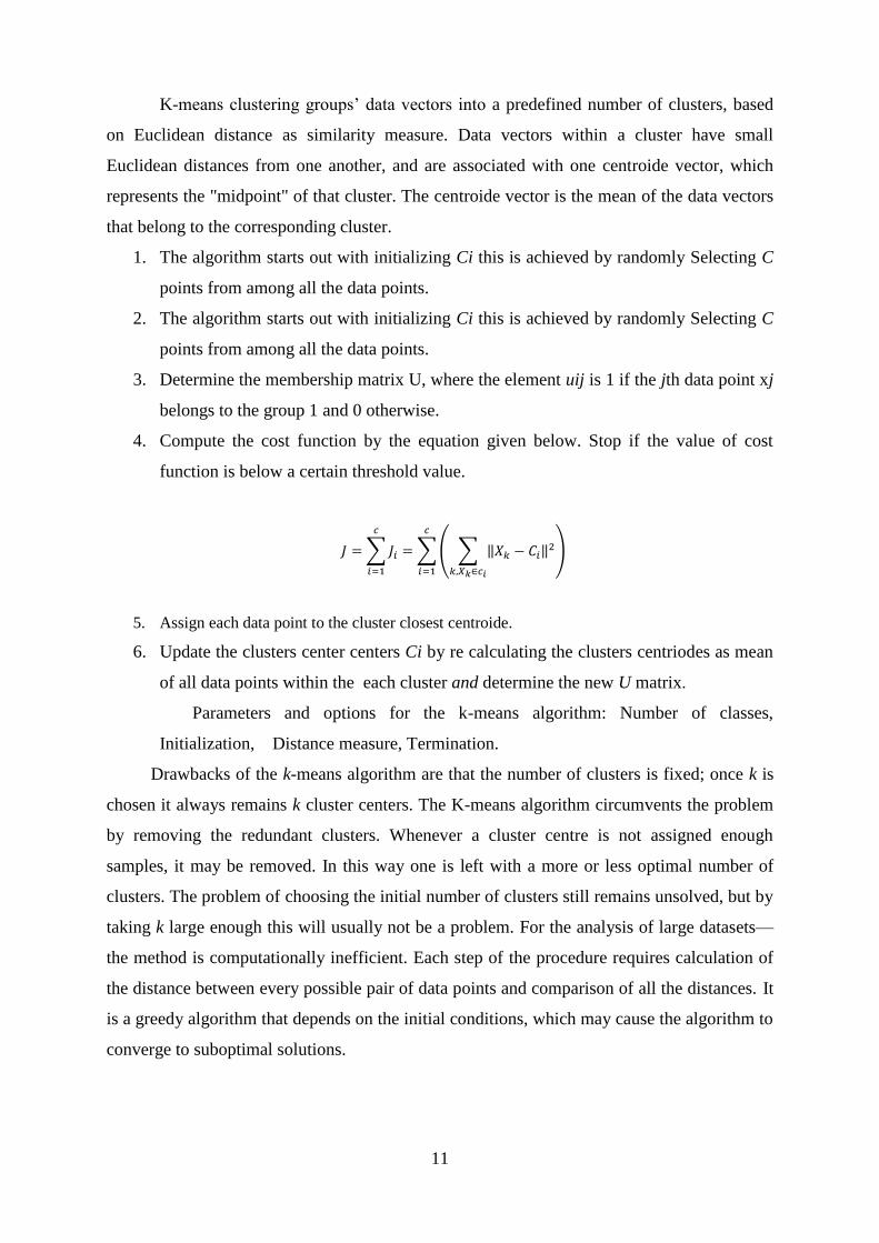
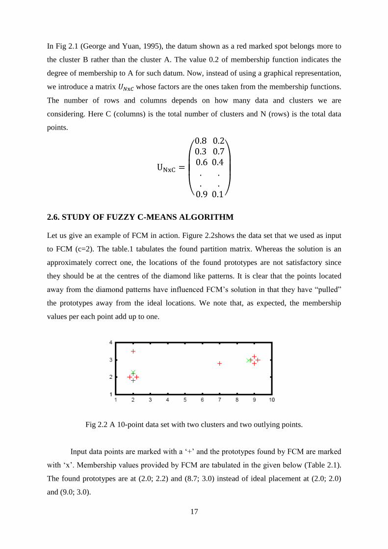
2.6. STUDY OF FUZZY C-MEANS ALGORITHM
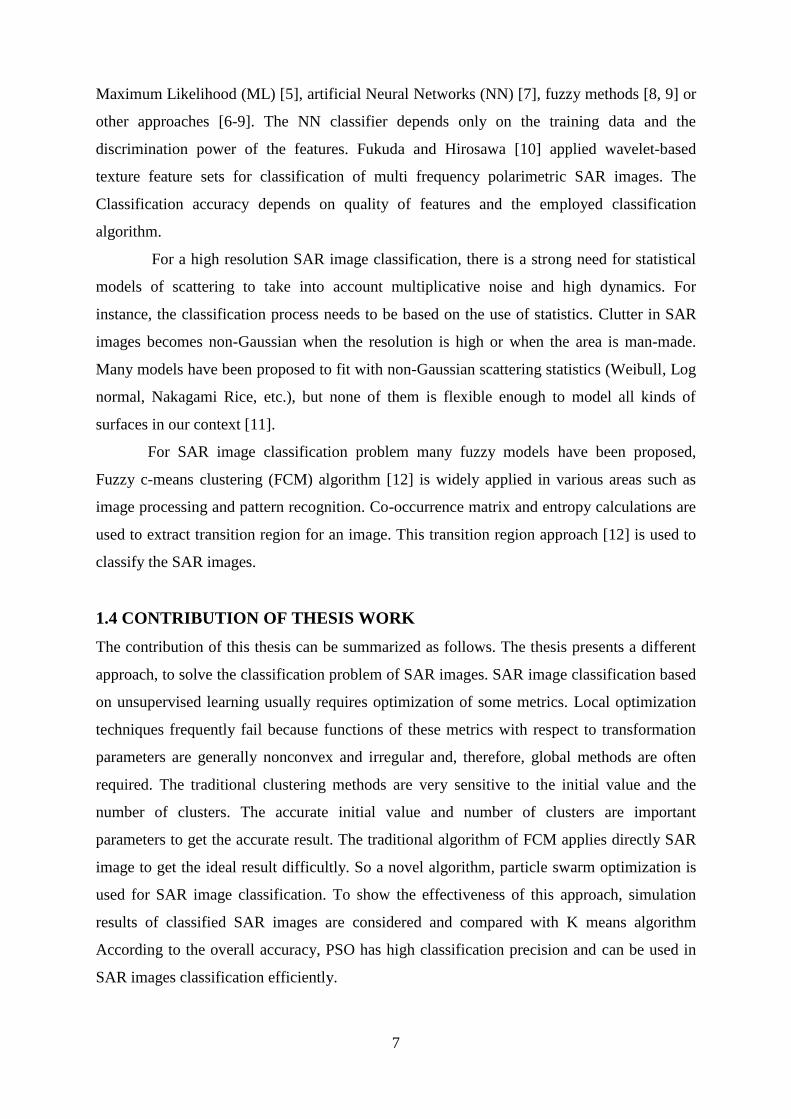
Let us give an example of FCM in action. Figure 2.2shows the data set that we used as input
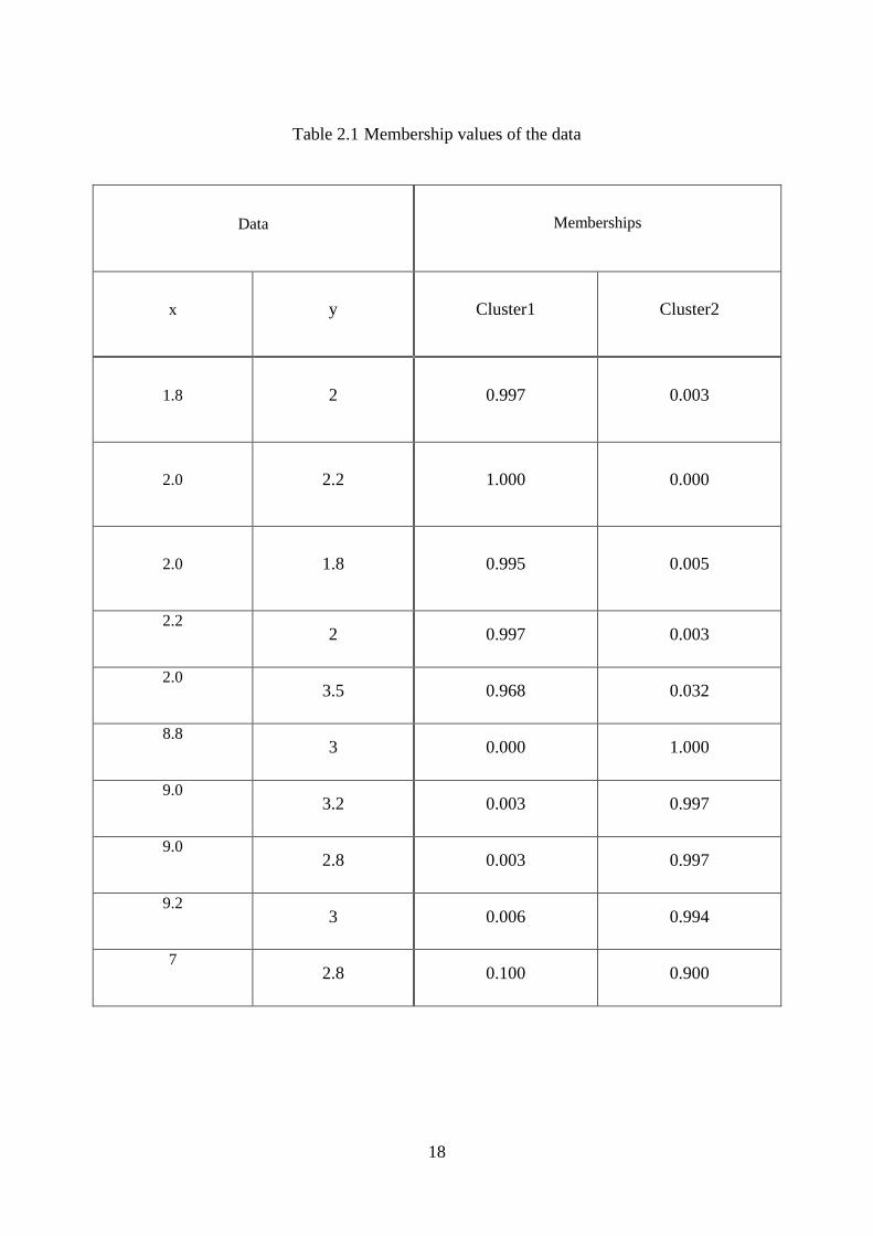
to FCM (c=2). The table.1 tabulates the found partition matrix. Whereas the solution is an
approximately correct one, the locations of the found prototypes are not satisfactory since
they should be at the centres of the diamond like patterns. It is clear that the points located
away from the diamond patterns have influenced FCM‘s solution in that they have ―pulled‖
the prototypes away from the ideal locations. We note that, as expected, the membership
values per each point add up to one.
Fig 2.2 A 10-point data set with two clusters and two outlying points.
Input data points are marked with a ‗+‘ and the prototypes found by FCM are marked
with ‗x‘. Membership values provided by FCM are tabulated in the given below (Table 2.1).
The found prototypes are at (2.0; 2.2) and (8.7; 3.0) instead of ideal placement at (2.0; 2.0)
and (9.0; 3.0).
18
Table 2.1 Membership values of the data
Data
Memberships
x
y Cluster1 Cluster2
1.8
2 0.997 0.003
2.0
2.2 1.000 0.000
2.0
1.8 0.995 0.005
2.2
2 0.997 0.003
2.0
3.5 0.968 0.032
8.8
3 0.000 1.000
9.0
3.2 0.003 0.997
9.0
2.8 0.003 0.997
9.2
3 0.006 0.994
7
2.8 0.100 0.900
19
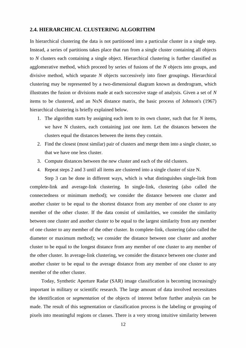
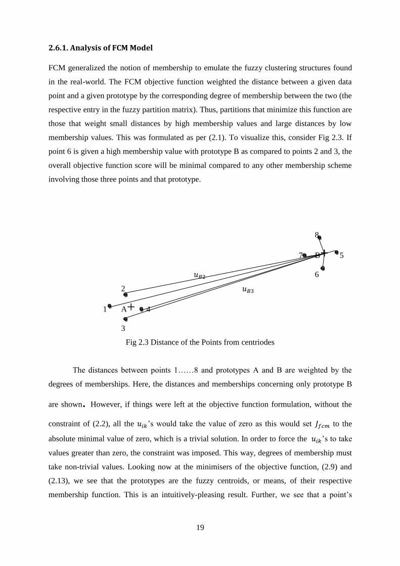
2.6.1. Analysis of FCM Model
FCM generalized the notion of membership to emulate the fuzzy clustering structures found
in the real-world. The FCM objective function weighted the distance between a given data
point and a given prototype by the corresponding degree of membership between the two (the
respective entry in the fuzzy partition matrix). Thus, partitions that minimize this function are
those that weight small distances by high membership values and large distances by low
membership values. This was formulated as per (2.1). To visualize this, consider Fig 2.3. If
point 6 is given a high membership value with prototype B as compared to points 2 and 3, the
overall objective function score will be minimal compared to any other membership scheme
involving those three points and that prototype.
8
7 B+ 5
6
2
1 A+ 4
3 Fig 2.3 Distance of the Points from centriodes
The distances between points 1……8 and prototypes A and B are weighted by the
degrees of memberships. Here, the distances and memberships concerning only prototype B
are shown. However, if things were left at the objective function formulation, without the
constraint of (2.2), all the ‘s would take the value of zero as this would set to the
absolute minimal value of zero, which is a trivial solution. In order to force the ‘s to take
values greater than zero, the constraint was imposed. This way, degrees of membership must
take non-trivial values. Looking now at the minimisers of the objective function, (2.9) and
(2.13), we see that the prototypes are the fuzzy centroids, or means, of their respective
membership function. This is an intuitively-pleasing result. Further, we see that a point‘s
20
membership with a given prototype is affected by how far that same point is to the other
prototypes. This is illustrated in Fig 2.3, where
(2.14)
This may cause counter-intuitive behavior in real-world data. If we observe Figure 2.3, we
notice that a point‘s membership degree is not a function of anything but its relative distances
to each prototype.
2.6.2. Strengths
The FCM algorithm has proven a very popular method of clustering for many reasons. In
terms of programming implementation, it is relatively straightforward. It employs an
objective function that is intuitive and easy-to-grasp. For data sets composed of hyper
spherically-shaped well-separated clusters, FCM discovers these clusters accurately.
Furthermore, because of its fuzzy basis, it performs robustly: it always converges to a
solution, and it provides consistent membership values.
2.6.3. Weaknesses
FCM technique has been used for classification of SAR images. But this method introduced
some errors in the classification results and was found to be very sensitive to initial cluster
centers.
CHAPTER3
SYNTHETIC APERTURE RADAR IMAGE CLASSIFICATION USING
PARTICLE SWARM OPTIMIZATION TECHNIQUE
21
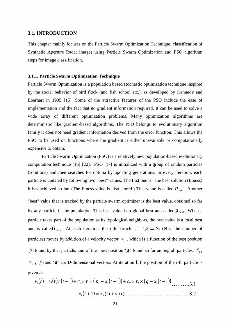
3.1. INTRODUCTION
This chapter mainly focuses on the Particle Swarm Optimization Technique, classification of
Synthetic Aperture Radar images using Particle Swarm Optimization and PSO algorithm
steps for image classification.
3.1.1. Particle Swarm Optimization Technique
Particle Swarm Optimization is a population based stochastic optimization technique inspired
by the social behavior of bird flock (and fish school etc.), as developed by Kennedy and
Eberhart in 1995 [15]. Some of the attractive features of the PSO include the ease of
implementation and the fact that no gradient information required. It can be used to solve a
wide array of different optimization problems. Many optimization algorithms are
deterministic like gradient-based algorithms. The PSO belongs to evolutionary algorithm
family it does not need gradient information derived from the error function. This allows the
PSO to be used on functions where the gradient is either unavailable or computationally
expensive to obtain.
Particle Swarm Optimization (PSO) is a relatively new population-based evolutionary
computation technique [16] [22]. PSO [17] is initialized with a group of random particles
(solutions) and then searches for optima by updating generations. In every iteration, each
particle is updated by following two "best" values. The first one is the best solution (fitness)
it has achieved so far. (The fitness value is also stored.) This value is called bestP . Another
"best" value that is tracked by the particle swarm optimizer is the best value, obtained so far
by any particle in the population. This best value is a global best and called bestg . When a
particle takes part of the population as its topological neighbors, the best value is a local best
and is called bestl . At each iteration, the i-th particle i = 1,2,.....N, (N is the number of
particles) moves by addition of a velocity vector iv , which is a function of the best position
ip found by that particle, and of the best position ‗g‘ found so far among all particles. ix ,
iv , ip and ‗g‘ are D-dimensional vectors. At iteration t, the position of the i-th particle is
given as
111 2211 txgrctxprctvtwtv iiiii ……….3.1
)()(1 tvtxtx iii ……………….……………..3.2

22
Where )(tw is the inertial weight, the 1c and 2c are acceleration constants, and the r (0,
1) are uniformly distributed random numbers. To keep the ix within reasonable bounds,
velocities are often clamped to a maximum velocity m axv : iv [- m axv m axv ]. The algorithm
makes use of two independent random sequences, )1,0(, 21 rr these sequences used to
affect the stochastic nature of the algorithm.
111 2211 txgrctxprctvtwtv iiiii ………3.3
The values of are scaled by constants 2,0 21 CC these constants are called the
acceleration coefficients, and they influence the maximum size of the step that a particle can
take in a single iteration. From the definition of the velocity update equation is clear that 2c
regularates the maximum step size in the direction of the global best particle, and 1c
regularates the maximum step size in the direction of the personal best of the particle. The
velocity is clamped to the range [- m axv m axv ], to reduce the likelihood that the particle might
leave the search space. if the search space is defined by the bounds maxmax, XX , then the
value of the maxV is typically set so that maxV =K* maxX where 0.11.0 K . The position of
each particle is updated using the velocity vector for that particle, so that
)()(1 tvtxtx iii
…………………3.4
It is important to realize that the velocity term models the rate of change in the position of the
particle. The change induced by the velocity update equation (3.3) there represents
acceleration, which explains why the constants 1c and 2c are called acceleration
coefficients. A brief description of how the algorithm works is as follows: Initially, some
particles are identified as the best particles in a neighborhood of particles, based on its fitness.
All the particles accelerated in the direction of this particle, but also in the direction of their
own best solutions that they have discovered previously. Occasionally the particles will
overshoot their target, exploring the search space beyond the current best particle. All
particles also have the opportunity to discover better particle en route, in which case the other
particles change direction and head towards the new ‗best’ particle. Since most functions
have some continuity, chances are that a good solution will be surrounded by equally, or
better, solutions. By approaching the current best solution from different solutions in search
space, the chances are good that these neighboring solutions will be discovered by some of
the particles.

23
3.2. SOCIAL BEHAVIOR
The velocity update equation is
111 2211 txgrctxprctvtwtv iiiii …….3.5
The third term in the velocity update equation, 122 txgrc i , represents the
social interaction between the particles. Social interaction between the particles is a form of
cooperation.
3.2.1 Co-operation
Clearwater et al. define cooperation as follows: ―Cooperation involves a collection of
agents that interact by communicating information to each other while solving a problem.‖
They further state that ―The information exchanged between agents may be incorrect, and
should sometimes alter the behavior of the agent receiving it.‖
3.3. RATE OF CONVERGENCE IMPROVEMENTS
Several techniques have been proposed for improving the rate of convergence of the PSO.
These proposals usually involve changes to the PSO update equations, without changing the
structure of the algorithm otherwise. This usually results in better local optimization
performance, sometimes with a corresponding decrease in performance on functions with
multiple local minima.
3.3.1. Inertia Weight
One of the most widely used improvements is the introduction of the ‗inertia weight’ by Shi
and Eberhart [18]. The ‗inertia weight’ is a scaling factor associated with the velocity during
the previous time step, resulting in a new velocity update equation, so that
111 2211 txgrctxprctvtwtv iiiii ….3.6
The original PSO velocity update equation can be obtained by setting w=1. Shi and Eberhart
investigated the effect of w values in the range [0, 1.4], as well as varying w over time [18].
Their results indicate that choosing w range [0.8 1.2] results in faster convergence, but that
larger w values (>1.2) result in more failures to convergence.
The inertia weight can be likened to the temperature parameter encountered in
simulated annealing algorithm. The simulated annealing algorithm has a process called the
temperature schedule that is used to gradually decrease the temperature of the system. The
24
higher the temperature, the greater the probability that the algorithm will explore a region
outside of basin of attraction of the current local minima. Therefore an adaptive inertia
weight can be seen as the equalent of a temperature schedule in the simulated annealing
algorithm.
3.3.2 Acceleration constants
The acceleration coefficients, 1c and 2c control how far a particle will move in a
single iteration. Typically these are both set to a value of 2.0, although it has been shown that
setting 21 cc can lead to improved performance.
The performance of PSO is dependent on the parameter settings: inertial weight )(tw
acceleration constants 1c and 2c , the maximum number of iterations T, and the
initialization of the population. The inertial weight is usually a monotonically decreasing
function of the iteration T.
3.4. CLASSIFICATION OF SAR IMAGE USING PSO
Omran [19] proposed the first clustering algorithm based on Particle Swarm Optimization
(PSO). In the PSO algorithm, the birds in a flock are symbolically represented as particles.
These particles can be considered as simple agents ―flying‖ through a problem space. A
particle‘s location in the multi-dimensional problem space represents one solution for the
problem. When a particle moves to a new location, a different problem solution is generated.
This solution is evaluated by a fitness function that provides a quantitative value of the
solution‘s utility.
3.4.1. PSO technique steps for image classification
The Particle Swarm Optimization technique composes of three main processes:
(1) Selecting training samples for every region in the SAR image.
(2) Training these samples using PSO, and obtain clustering center of every region.
(3) Finally, output the classification result of SAR image according to clustering
center obtained.
The new method can be implemented as follows:
Step 1: Selecting training samples for every region in the image according to the
number of classes.
Step 2: Generate the initial swarm, ,)0()......0(),0()0( 21 mxxxX generate the initial
25
velocity. Set t=0, bestii pfbest , ,,.....2,1 mi bestgfbest .
Step 3: Calculate the fitness of all the particles in )(tX as follows.
For SAR image classification problem, the clustering center
mcccC ,....., 21 is the mean value of all particles. The fitness of particle
,)()......(),()( 21 txtxtxtx n is defined as:
7.3......................)(1
i
n
i
i ctxtxfitness
Step 4: Update position and velocity of all the particles as equation (3.1) and (3.2) and
set )1( tX to be the resulting swarm
Step 5: For all the particles in )1( tX , if ii fbesttxfitness ,then set
))(( txfitnessfbest ii , );1( txp ii
if fbesttxfitness i then ))(( txfitnessfbest i , 1 txg i .
Step 6: If stop condition is satisfied, export )1( tX as the output of the algorithm,
Stop.
Otherwise, t=t+1, go to Step 3. Here the stop condition is to set as the maximum number
of iterations T.
Step 7: Get the optimal clustering center, which is the center of last swarm obtained.
Step 8: Repeat Step 2 to Step 7 for every class, get the optimal clustering center for
every class.
Step 9: After training all the regions, calculate the distance between all pixels and
Clustering centers, assign every pixel to one class with the least distance.
3.4.2. CONCLUSION
The objective of the PSO clustering algorithm is to obtain the proper centroids of clusters for
minimizing the intra-cluster distance as well as maximizing the distance between clusters.
The PSO algorithm performs a globalized searching for solutions whereas most other
partitional clustering procedures perform a localized searching [20]. In localized searching,
the solution obtained is usually located in the vicinity of the solution obtained in the previous
step.
CHAPTER 4
CLASSIFICATION ACCURACY ASSESSMENT
26
4.1. INTRODUCTION
In this Chapter, accuracy assessment procedure is described. The accuracy of spatial data has
been defined as ―The closeness of results of observations, computations, or estimates to the
true values or the values accepted as being true".
4.1.1 Accuracy Assessment
Accuracy assessment is an important step in the process of analyzing remote sensing
data. Remote sensing products can serve as the basis for economical decisions. Potential
users have to know about the reliability of the data when confronted with maps derived from
remote sensing data. Accuracy defines "correctness"; it measures the agreement between a
standard assumed to be correct and a classified image of unknown quality. If the image
classification corresponds closely with the standard, it is said to be accurate. There are two
forms of measuring accuracy; the first one is the using of reference map that is assumed to be
the "correct" map and to be compared with the map to be evaluated. We have used the second
form of accuracy, site-specific accuracy that is based on the detailed assessment between two
maps at specific locations; it is possible to compile an error matrix that is necessary for any
serious study of accuracy. The most common way to express classification accuracy is the
preparation of an error matrix also known as confusion matrix or contingency matrix. Such
matrices show the cross tabulation of the classified land cover and the actual land cover
revealed by sample site results. Different measures and statistics can be derived from the
values in an error matrix. The basic form of an error matrix and non statistical measures are
described in 4.2.
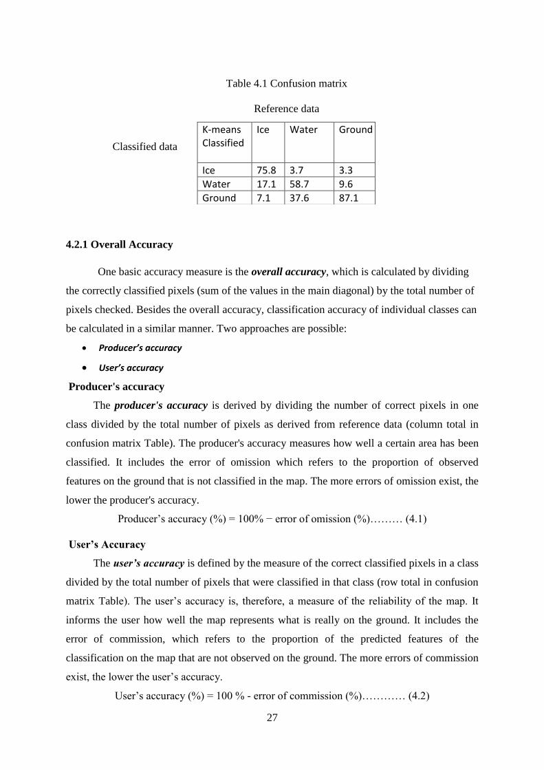
4.2 CONFUSION MATRIX
A confusion matrix lists the values of known cover types of the reference data in the
columns and of the classified data in the rows (Table 4.1). The main diagonal of the matrix
lists the correctly classified pixels. One benefit of a confusion matrix is that it is easy to see if
the system is confusing two classes (i.e. commonly mislabeling one as another). A confusion
matrix contains information about actual and predicted classifications done by a classification
system. Performance of such systems is commonly evaluated using the data in the matrix.
27
Table 4.1 Confusion matrix
Reference data
Classified data
4.2.1 Overall Accuracy
One basic accuracy measure is the overall accuracy, which is calculated by dividing
the correctly classified pixels (sum of the values in the main diagonal) by the total number of
pixels checked. Besides the overall accuracy, classification accuracy of individual classes can
be calculated in a similar manner. Two approaches are possible:
Producer’s accuracy
User’s accuracy
Producer's accuracy
The producer's accuracy is derived by dividing the number of correct pixels in one
class divided by the total number of pixels as derived from reference data (column total in
confusion matrix Table). The producer's accuracy measures how well a certain area has been
classified. It includes the error of omission which refers to the proportion of observed
features on the ground that is not classified in the map. The more errors of omission exist, the
lower the producer's accuracy.
Producer‘s accuracy (%) = 100% − error of omission (%)……… (4.1)
User‟s Accuracy
The user’s accuracy is defined by the measure of the correct classified pixels in a class
divided by the total number of pixels that were classified in that class (row total in confusion
matrix Table). The user‘s accuracy is, therefore, a measure of the reliability of the map. It
informs the user how well the map represents what is really on the ground. It includes the
error of commission, which refers to the proportion of the predicted features of the
classification on the map that are not observed on the ground. The more errors of commission
exist, the lower the user‘s accuracy.
User‘s accuracy (%) = 100 % - error of commission (%)………… (4.2)
K-means Classified
Ice Water Ground
Ice 75.8 3.7 3.3
Water 17.1 58.7 9.6
Ground 7.1 37.6 87.1
28
4.3. KAPPA COEFFICIENT
The Kappa coefficient was introduced to the remote sensing community in the early
1980s (Congalton and Mead, 1983) and has become a widely used measure for classification
accuracy. It was recommended as a standard by Rosenfield and Fitzpatrick-Lins (1986). The
kappa coefficient is a measure of overall agreement of a matrix. In contrast to the overall
accuracy the ratio of the sum of diagonal values to total number of cell counts in the matrix
the Kappa coefficient takes also non-diagonal elements into account (Rosenfield and
Fitzpatrick, 1986). Kappa coefficient is a statistical measure of inter-rater reliability (Cohen,
1960). It measures the proportion of agreement after chance agreements have been removed
from considerations. It is generally thought to be a more reliable measure than simple percent
agreement calculation, since К takes into account the agreement occurring by chance.
The equation for the kappa coefficient is given as
r
ii
Xi
XN
r
ii
Xr
ii
Xii
XN
K
1
2
1 1ˆ ……………. (4.3)
Where
r = number of rows and columns in error matrix,
N = total number of observations,
iiX = observation in row i and column i,
iX = marginal total of row i, and
iX = marginal total of column i.
Another formula to find kappa coefficient is
ep
ep
op
K
1ˆ ……………. .…………………………(4.4)
Where
o
p Accuracy of the observed agreement, N
X ii
e
p Estimate of chance agreement, 2N
XX ii
A table for interpreting К values is given by Landis & Koch (1977). Although it is based on
personal opinion and by no means universally accepted, it is presented here (Table 4.2), as

29
many studies refer to it (Altmann, 1991; Kulbach, 1997; Ortiz et al., 1997; Komagata, 2002;
Oehmichen, 2007).
Table - 4.2 Interpretation of K-values
For example a Kappa coefficient value of 0.67 can be thought of as an indication that an
observed classification is 67 percent one resulting from chance.
Kappa value[%] Interpretation
<0 Poor agreement
0 to 20 Slight agreement
20 to 40 Fair agreement
40 to 60 Moderate agreement
60 to 80 Substantial agreement
80 to 100 Almost perfect agreement

CHAPTER 5
SIMULATIONS AND RESULTS
30
In this thesis work, we have considered synthetic aperture radar images. The SAR images
are classified by using 3 different algorithms, namely Particle Swarm Optimization (PSO),
Fuzzy C-Means algorithm (FCM) and K-means algorithm. The performance of these three
algorithms is compared using ―Confusion Matrix‖ or error matrix, overall accuracy and
Kappa coefficient. The obtained results showed that, among these three algorithms the PSO
algorithm gives better classification results over the FCM and K-means classification
algorithms.
The fig 5.1.2(a) shows the SAR image courtesy of The Reo Grande River at Albuquerque,
New Mexico; which was taken from Sandia National Laboratories SAR imagery. The survey
area is part of river, and the primary objective of this survey was to discriminate various
objects. The observed image was expected to fall into three classes: river, vegetation and
crop. The corresponding PSO classified, FCM classified and K-means classified images are
shown in figures 5.1.2(b), 5.1.2(c) and 5.1.2(d) respectively. Each simulation took 100
iterations to get successful results.
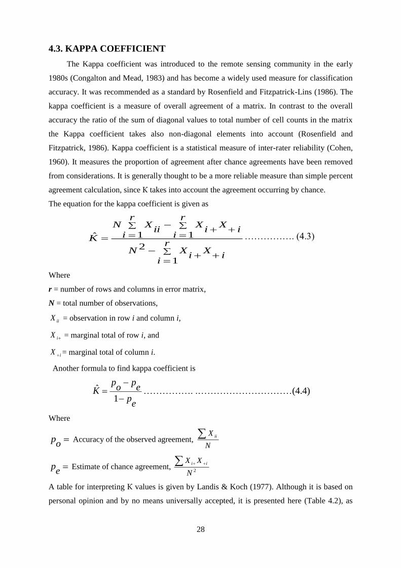
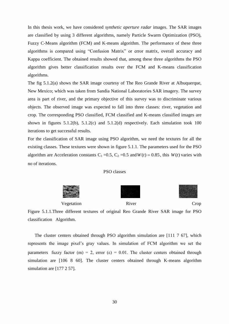
For the classification of SAR image using PSO algorithm, we need the textures for all the
existing classes. These textures were shown in figure 5.1.1. The parameters used for the PSO
algorithm are Acceleration constants C1 =0.5, C2 =0.5 and 85.0)( tW , this )(tW varies with
no of iterations.
PSO classes
Vegetation River Crop
Figure 5.1.1.Three different textures of original Reo Grande River SAR image for PSO
classification Algorithm.
The cluster centers obtained through PSO algorithm simulation are [111 7 67], which
represents the image pixel‘s gray values. In simulation of FCM algorithm we set the
parameters fuzzy factor (m) = 2, error (ε) = 0.01. The cluster centers obtained through
simulation are [106 8 60]. The cluster centers obtained through K-means algorithm
simulation are [177 2 57].

31
Figure5.1.2 (a) The Reo Grande River SAR Figure 5.1.2(b) The PSO classified Image
Image
Figure 5.1.2(c) The FCM classified Image Figure 5.1.2(d) The K-means classified Image
Vegetation River Crop
SAR image PSO - Classified Image
FCM - Classified Image K-means Classified Image
32
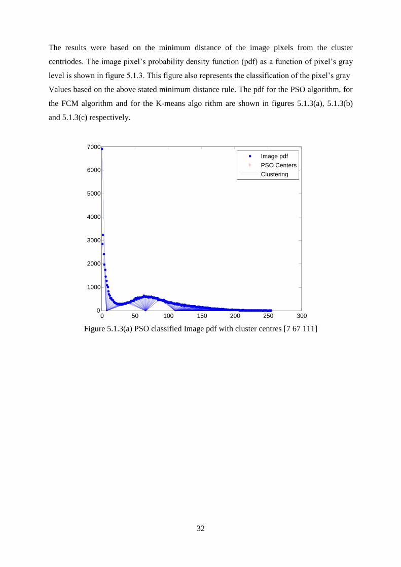
The results were based on the minimum distance of the image pixels from the cluster
centriodes. The image pixel‘s probability density function (pdf) as a function of pixel‘s gray
level is shown in figure 5.1.3. This figure also represents the classification of the pixel‘s gray
Values based on the above stated minimum distance rule. The pdf for the PSO algorithm, for
the FCM algorithm and for the K-means algo rithm are shown in figures 5.1.3(a), 5.1.3(b)
and 5.1.3(c) respectively.
Figure 5.1.3(a) PSO classified Image pdf with cluster centres [7 67 111]
0 50 100 150 200 250 300 0
1000
2000
3000
4000
5000
6000
7000
Image pdf PSO Centers Clustering
33
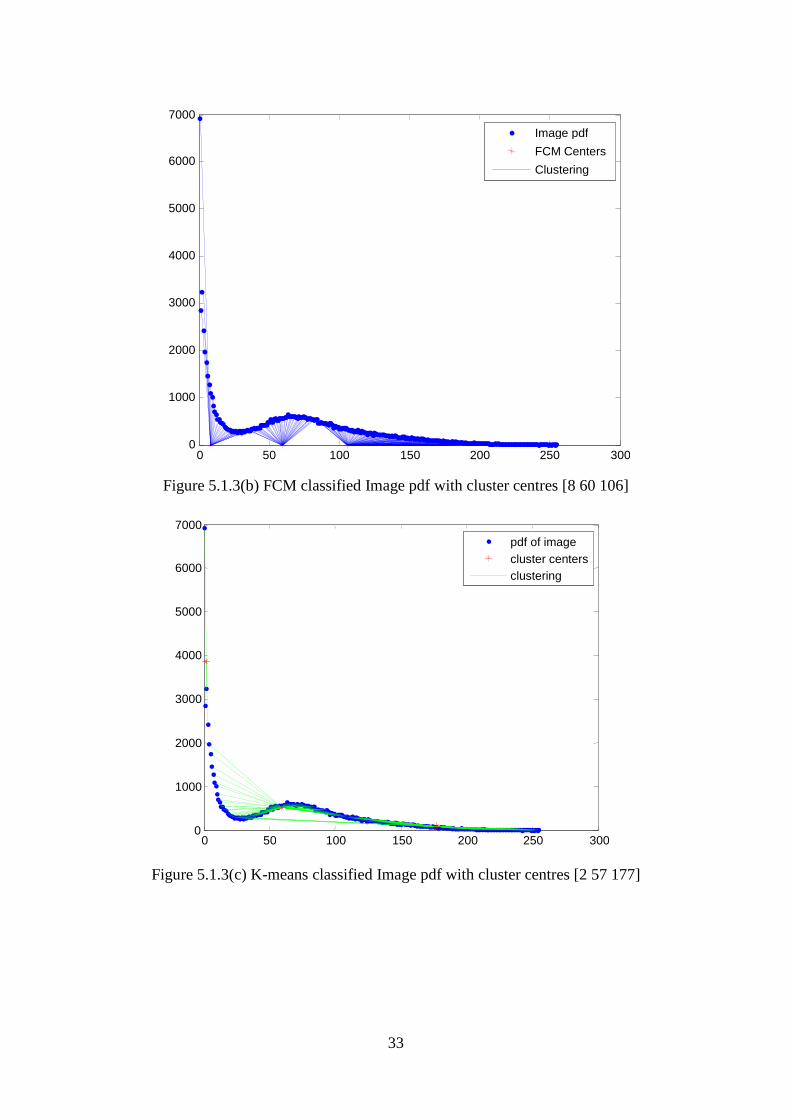
Figure 5.1.3(b) FCM classified Image pdf with cluster centres [8 60 106]
Figure 5.1.3(c) K-means classified Image pdf with cluster centres [2 57 177]
0 50 100 150 200 250 300 0
1000
2000
3000
4000
5000
6000
7000
pdf of image cluster centers clustering
0 50 100 150 200 250 300 0
1000
2000
3000
4000
5000
6000
7000
Image pdf FCM Centers Clustering
34
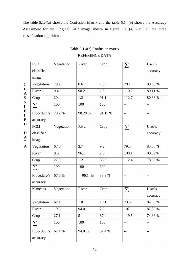
The table 5.1.4(a) shows the Confusion Matrix and the table 5.1.4(b) shows the Accuracy
Assessment for the Original SAR image shown in figure 5.1.1(a) w.r.t. all the three
classification algorithms.
Table 5.1.4(a) Confusion matrix
REFERENCE DATA
PSO
classified
image
Vegetation River Crop User‘s
accuracy
Vegetation 70.2 0.6 7.3 78.1 89.88 %
River 9.4 98.2 2.6 110.2 89.11 %
Crop 20.4 1.2 91.1 112.7 80.83 %
100 100 100 -- --
Procedure‘s
accuracy
70.2 % 98.20 % 91.10 % -- --
FCM
classified
image
Vegetation River Crop User‘s
accuracy
Vegetation 67.6 2.7 9.2 79.5 85.00 %
River 9.5 96.1 2.5 108.1 88.89%
Crop 22.9 1.2 88.3 112.4 78.55 %
100 100 100 -- --
Procedure‘s
accuracy
67.6 % 96.1 % 88.3 % -- --
K-means Vegetation River Crop User‘s
accuracy
Vegetation 62.4 1.0 10.1 73.5 84.89 %
River 10.5 94.0 2.5 107 87.85 %
Crop 27.1 5 87.4 119.5 74.38 %
100 100 100 -- --
Procedure‘s
accuracy
62.4 % 94.0 % 97.4 % -- --
C
L
A
S
S
I
F
I
E
D
D
A
T
A
35
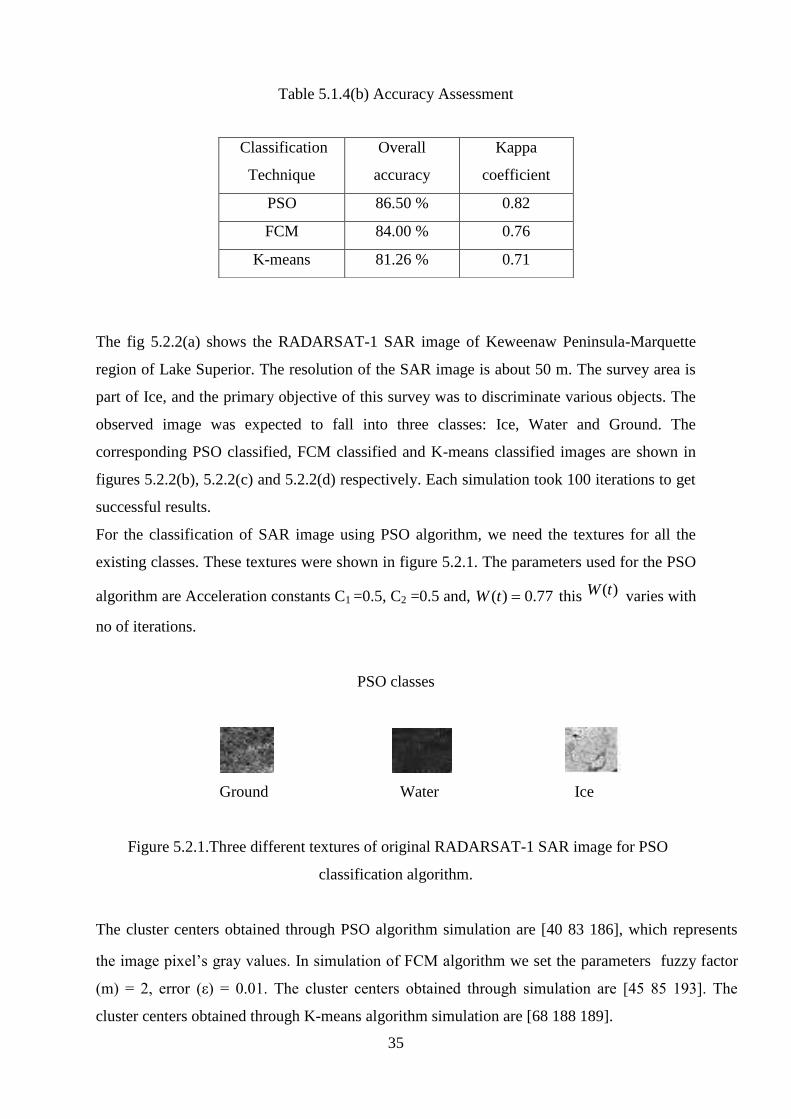
Table 5.1.4(b) Accuracy Assessment
The fig 5.2.2(a) shows the RADARSAT-1 SAR image of Keweenaw Peninsula-Marquette
region of Lake Superior. The resolution of the SAR image is about 50 m. The survey area is
part of Ice, and the primary objective of this survey was to discriminate various objects. The
observed image was expected to fall into three classes: Ice, Water and Ground. The
corresponding PSO classified, FCM classified and K-means classified images are shown in
figures 5.2.2(b), 5.2.2(c) and 5.2.2(d) respectively. Each simulation took 100 iterations to get
successful results.
For the classification of SAR image using PSO algorithm, we need the textures for all the
existing classes. These textures were shown in figure 5.2.1. The parameters used for the PSO
algorithm are Acceleration constants C1 =0.5, C2 =0.5 and, 77.0)( tW this )(tW varies with
no of iterations.
PSO classes
Ground Water Ice
Figure 5.2.1.Three different textures of original RADARSAT-1 SAR image for PSO
classification algorithm.
The cluster centers obtained through PSO algorithm simulation are [40 83 186], which represents
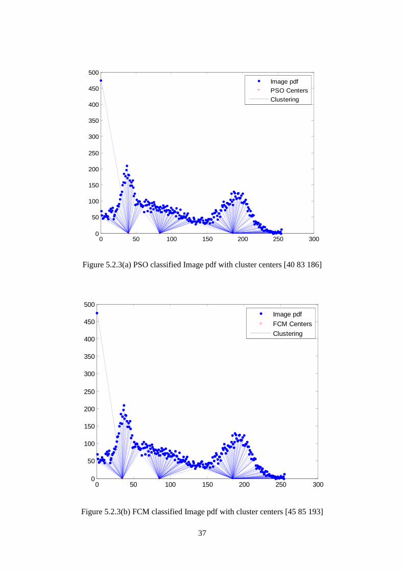
the image pixel‘s gray values. In simulation of FCM algorithm we set the parameters fuzzy factor
(m) = 2, error (ε) = 0.01. The cluster centers obtained through simulation are [45 85 193]. The
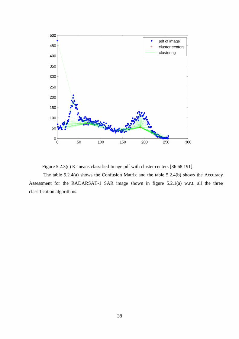
cluster centers obtained through K-means algorithm simulation are [68 188 189].
Classification
Technique
Overall
accuracy
Kappa
coefficient
PSO 86.50 % 0.82
FCM 84.00 % 0.76
K-means 81.26 % 0.71

36
Figure 5.2.2(a) RADARSAT-1 SAR image Figure 5.2.2(b) The PSO classified Image
Figure 5.2.2 (c) The FCM classified Image Figure 5.2.2(d) The K-means classified Image
Ground Water Ice
The image pixel‘s probability density function (pdf) as a function of pixel‘s gray level is
shown in figure 5.2.3. This figure also represents the classification of the pixel‘s gray values
based on the above stated minimum distance rule. The pdf for the PSO algorithm, for the
FCM algorithm and for the K-means algorithm are shown in figures 5.2.3(a), 5.2.3(b) and
5.2.3(c) respectively.
PSO - Classified Image SAR image
FCM- Classified Image K-means Classified Image
37
Figure 5.2.3(a) PSO classified Image pdf with cluster centers [40 83 186]
Figure 5.2.3(b) FCM classified Image pdf with cluster centers [45 85 193]
0 50 100 150 200 250 3000
50
100
150
200
250
300
350
400
450
500
Image pdf
PSO Centers
Clustering
0 50 100 150 200 250 3000
50
100
150
200
250
300
350
400
450
500
Image pdf
FCM Centers
Clustering
38
Figure 5.2.3(c) K-means classified Image pdf with cluster centers [36 68 191].
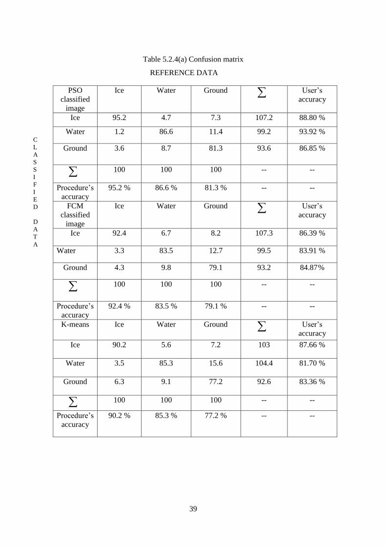
The table 5.2.4(a) shows the Confusion Matrix and the table 5.2.4(b) shows the Accuracy
Assessment for the RADARSAT-1 SAR image shown in figure 5.2.1(a) w.r.t. all the three
classification algorithms.
0 50 100 150 200 250 3000
50
100
150
200
250
300
350
400
450
500
pdf of image
cluster centers
clustering
39
Table 5.2.4(a) Confusion matrix
REFERENCE DATA
PSO
classified
image
Ice Water Ground User‘s
accuracy
Ice 95.2 4.7 7.3 107.2 88.80 %
Water 1.2 86.6 11.4 99.2 93.92 %
Ground 3.6 8.7 81.3 93.6 86.85 %
100 100 100 -- --
Procedure‘s
accuracy
95.2 % 86.6 % 81.3 % -- --
FCM
classified
image
Ice Water Ground User‘s
accuracy
Ice 92.4 6.7 8.2 107.3 86.39 %
Water 3.3 83.5 12.7 99.5 83.91 %
Ground 4.3 9.8 79.1 93.2 84.87 %
100 100 100 -- --
Procedure‘s
accuracy
92.4 % 83.5 % 79.1 % -- --
K-means Ice Water Ground User‘s
accuracy
Ice 90.2 5.6 7.2 103 87.66 %
Water 3.5 85.3 15.6 104.4 81.70 %
Ground 6.3 9.1 77.2 92.6 83.36 %
100 100 100 -- --
Procedure‘s
accuracy
90.2 % 85.3 % 77.2 % -- --
C
L
A
S
S
I
F
I
E
D
D
A
T
A

40
Table 5.2.4(b) Accuracy Assessment
Technique Overall
accuracy
Kappa coefficient
PSO 87.70 % 0.81
FCM 85.00 % 0.77
K-means 84.23 % 0.76
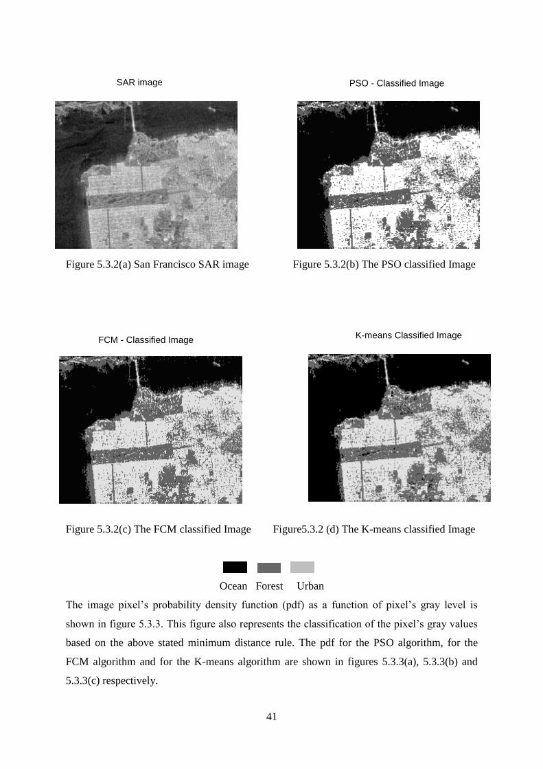
The fig 5.3.2(a) shows the L-band San Francisco SAR image. The survey area is part of
Ocean, and the primary objective of this survey was to discriminate various objects. The
observed image was expected to fall into three classes: Ocean, Forest and Urban. The
corresponding PSO classified, FCM classified and K-means classified images are shown in
figures 5.3.2(b), 5.3.2(c) and 5.3.2(d) respectively. Each simulation took 100 iterations to get
successful results.
For the classification of SAR image using PSO algorithm, we need the textures for all the
existing classes. These textures were shown in figure 5.3.1. The parameters used for the PSO
algorithm are Acceleration constants C1 =0.5, C2 =0.5 and, 79.0)( tW this )(tW varies with
no of iterations.
PSO classes
Ocean Forest Urban
Figure 5.3.1.Three different textures of original L-band San Francisco SAR image for PSO
classification algorithm.
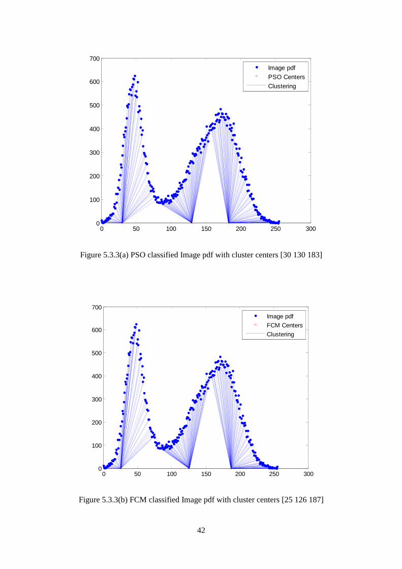
The cluster centers obtained through PSO algorithm simulation are [30 130 183], which
represents the image pixel‘s gray values. In simulation of FCM algorithm we set the
parameters fuzzy factor (m) = 2, error (ε) = 0.01. The cluster centers obtained through
simulation are C= [25 126 187]. The cluster centers obtained through K-means algorithm
simulation are [83 127 232].
41
SAR image
Figure 5.3.2(a) San Francisco SAR image Figure 5.3.2(b) The PSO classified Image
Figure 5.3.2(c) The FCM classified Image Figure5.3.2 (d) The K-means classified Image
Ocean Forest Urban
The image pixel‘s probability density function (pdf) as a function of pixel‘s gray level is
shown in figure 5.3.3. This figure also represents the classification of the pixel‘s gray values
based on the above stated minimum distance rule. The pdf for the PSO algorithm, for the
FCM algorithm and for the K-means algorithm are shown in figures 5.3.3(a), 5.3.3(b) and
5.3.3(c) respectively.
PSO - Classified Image
FCM - Classified Image K-means Classified Image
42
Figure 5.3.3(a) PSO classified Image pdf with cluster centers [30 130 183]
Figure 5.3.3(b) FCM classified Image pdf with cluster centers [25 126 187]
0 50 100 150 200 250 3000
100
200
300
400
500
600
700
Image pdf
PSO Centers
Clustering
0 50 100 150 200 250 3000
100
200
300
400
500
600
700
Image pdf
FCM Centers
Clustering
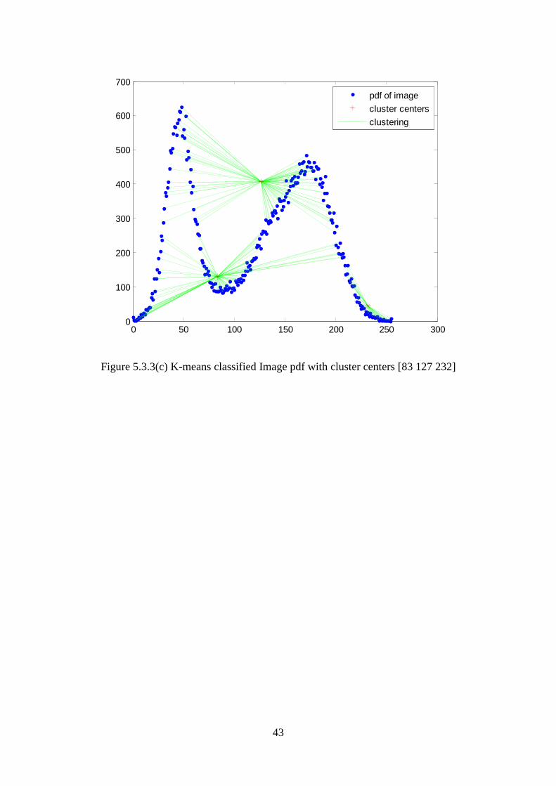
43
Figure 5.3.3(c) K-means classified Image pdf with cluster centers [83 127 232]
0 50 100 150 200 250 3000
100
200
300
400
500
600
700
pdf of image
cluster centers
clustering
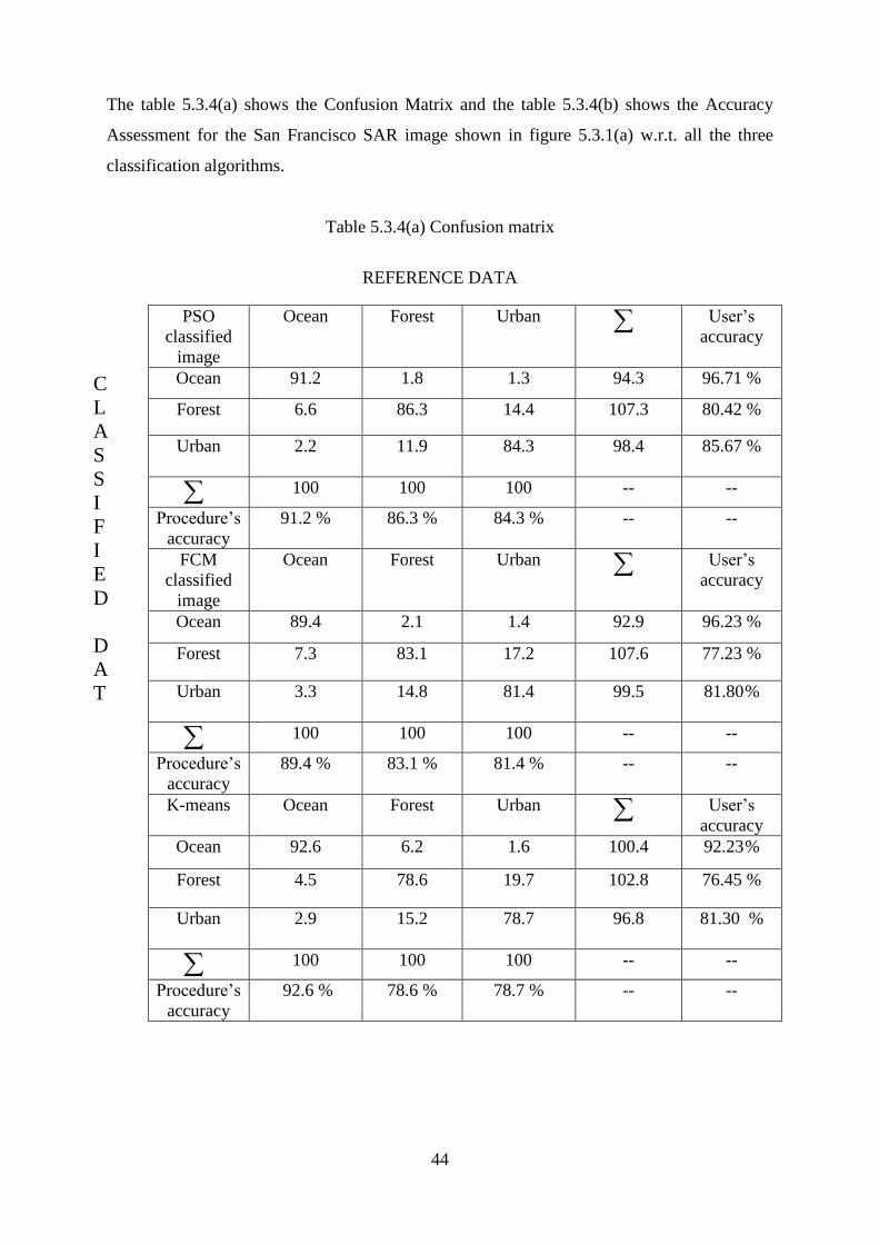
44
The table 5.3.4(a) shows the Confusion Matrix and the table 5.3.4(b) shows the Accuracy
Assessment for the San Francisco SAR image shown in figure 5.3.1(a) w.r.t. all the three
classification algorithms.
Table 5.3.4(a) Confusion matrix
REFERENCE DATA
PSO
classified
image
Ocean Forest Urban
User‘s
accuracy
Ocean 91.2 1.8 1.3 94.3 96.71 %
Forest 6.6 86.3 14.4 107.3 80.42 %
Urban
2.2 11.9 84.3 98.4 85.67 %
100 100 100 -- --
Procedure‘s
accuracy
91.2 % 86.3 % 84.3 % -- --
FCM
classified
image
Ocean Forest Urban
User‘s
accuracy
Ocean 89.4 2.1 1.4 92.9 96.23 %
Forest 7.3 83.1 17.2 107.6 77.23 %
Urban
3.3 14.8 81.4 99.5 81.80 %
100 100 100 -- --
Procedure‘s
accuracy
89.4 % 83.1 % 81.4 % -- --
K-means Ocean Forest Urban
User‘s
accuracy
Ocean 92.6 6.2 1.6 100.4 92.23 %
Forest 4.5 78.6 19.7 102.8 76.45 %
Urban
2.9 15.2 78.7 96.8 81.30 %
100 100 100 -- --
Procedure‘s
accuracy
92.6 % 78.6 % 78.7 % -- --
C
L
A
S
S
I
F
I
E
D
D
A
T
A

45
Table 5.3.4(b) Accuracy Assessment
Technique Overall
accuracy
Kappa coefficient
PSO 87.26 % 0.80
FCM 84.63 % 0.76
K-means 83.30 % 0.74

CHAPTER 6
CONCLUSION
46
6.1 CONCLUSIONS
This chapter summarizes and concludes the investigation of SAR image classification
presented in this thesis. It emphasizes the main points of the theoretic and practical work
performed during this project and presents conclusions that can be drawn from the results.
Some image classification methods have been studied. All are given acceptable results.
In this thesis a novel algorithm based on the Particle Swarm Optimization, was
designed for SAR images classification. The new algorithm is successfully applied for
classification of SAR images. The experimental results consistently show that the proposed
algorithm has high classification precision. When compared with other two classifiers, K-
means, and FCM, the average performance of PSO is better than them. The performance is
evaluated by accuracy assessment.
In terms of image classification accuracy evaluation, attention was mainly focused on
subjective methods of evaluation. Confusion matrix, overall accuracy and Kappa coefficient
are the main considerations in organizing and running subjective tests for method of image
classification accuracy evaluation.
The PSO clustering algorithm is used to obtain the proper centroids of clusters for
minimizing the intra-cluster distance as well as maximizing the distance between clusters.
The effectiveness of PSO algorithm was evaluated by accuracy assessment. We achieved
more accuracy with PSO because it is a global searching technique. The performance of PSO
technique is found to be satisfactory and the performance of outperformed FCM and K-
means technique. The classification results are validated with various SAR images.
6.2 FUTURE WORK
Classification of SAR images using PSO technique requires training sample of every
region in the image. So the number of classes is assumed to be known. Hence this problem
can be considered to semi-supervised. Future work can be extended by considering the
classification problem to be completely unsupervised where the no. of classes are unknown
this problem is both pursuing and computational burden is to be considered along with other
subjective tests for performance measurement.
47
REFERENCES
[1] C. W. Sherwin, J. P. Ruina, and R. D. Rawcliffe, ―Some early developments in synthetic
aperture radar systems,‖ IRE Trans .Mil. Electron. Vol. MIL-6, pp. 111-1 15, Apr. 1962.
[2] Gao Lan, Zhan Jianqiang, Lu Ling, Song Wenwu, ―Segmentation of SAR image in
electromagnetic environment based on fractal theory‖ Asia-Pacific Conference on
Environmental Electromagnetics, CEEM‘ NOV 4-7,2003 Hangzhou, CHINA.
[3] Saevarsson, B.B, Sveinsson, J.R, Benediktsson J.A, ―Combined Wavelet and Curvelet
denoising of SAR Images‖, IEEE Transactions on Geosciences and Remote Sensing, Vol6,
pp. 4235-4238, Sept 2004.
[4] Zheng-Wen Xu, JianWu and Zhen-Sen Wu, “A survey of ionospheric effects on space-
based radar” Institute of Physics Publishing, Waves Random Media 14 (2004) S189–
S273.[5] Lee J S, Grunes M R, Kwok R. ―Classification of multi-look polarimetric SAR
imagery based on complex Wishart distribution‖, Int. J. Remote Sensing, 1994, 15(11): 2299-
2311.
[6] Van Zyl J J. ―Unsupervised classification of scattering behavior using radar polarimetry
data‖,IEEE Trans. Geosci. Remote Sensing, 1989, 27(1): 36-45.
[7] Bischof H, Schneider W, Pinz A J. ―Multispectral classification of landsat-images using
neural networks‖, IEEE Trans. Geosci. Remote Sensing, 1992, 30(3): 482-490.
[8] Chen C T, Chen K S, Lee J S. ―The use of fully polarimetric information for the fuzzy
neural classification of SAR images‖, IEEE Trans. Geosci. Remote Sensing, 2003, 41(9 Part
I): 2089-2100.
[9] Du L, Lee J S. ―Fuzzy classification of earth terrain covers using complex polarimetric
SAR data‖, International Journal of Remote Sensing, 1996, 17(4): 809-826.
[10] Fukuda S, Hirosawa H. ―A wavelet-based texture feature set applied to classification of
multi frequency polarimetric SAR images‖. IEEE Trans. Geosci. Remote Sensing, 1999,
37(5): 2282-2286.
[11] Céline Tison, Jean-Marie Nicolas, Florence Tupin, and Henri Maître.―A new Statistical
Model for Markovian Classification of Urban Areas in High-Resolution SAR Images‖ IEEE
Trans. Geoscience and Remote sensing, Vol. 42, No. 10, October 2004.
[12] Lan Gao, Feng pan, XiaoQuan Li.A ―New Fuzzy Unsupervised Classification Method
for SAR Images‖ IEEE Trans.2006.
[13] H. Frigui and R. Krishnapuram, ―A robust competitive clustering algorithm with
applications in computer vision,‖ IEEE Transactions on Pattern Analysis and Machine
Intelligence, vol. 21, no. 5, pp. 450–465, 1999.

48
[14] J. Zhang Y. Leung and Z. Xu, ―Clustering by space-space filtering,‖ IEEE Transactions
on Pattern Analysis and Machine Intelligence, vol. 22, no. 12, pp. 1396–1410, 2000.
[15] Russ C.Eberhart, J.kennedy, ―A new optimizer using Particle Swarm Theory‖, In
proceedings of the Sixth International Symposium on Micro Machine and Human Science,
Pages 39-43, Nagoya, Japan, 1995.
[16] J. Kennedy, R. C. Eberhart, "Particle swarm optimization", Proc. IEEE Int. Conf
Neural Networks, vol. 4, Perth, Australia, Dec. 1995, pp. 1942-1948.
[17] J. Kennedy, R. C. Eberhart, ―Swarm Intelligence‖, Morgan Kaufman, San Mateo, Ca,
2001.
[18] Y.Shi, Russ C.Eberhart, ―A Modified Particle Swarm Optimizer‖, IEEE International
Conference of Evolutionary Computation, Anchorage, Alaska, May 1998.
[19] A. Salman M. Omran and A. Engelbrecht, ―Image classification using particle swarm
optimization,‖ in Conference on Simulated Evolution and Learning, Singapore, 2002, vol. 1,
pp. 370–374.
[20] Xiaohui Cui, Thomas E. Potok, Paul Palathingal, ―Document Clustering using Particle
Swarm Optimization‖, Applied Software Engineering Research Group Computational
Sciences and Engineering Division Oak Ridge National Laboratory.