Classification of Sperm Whale Clicks (Physeter ...

Algorithms 2009, 2, 1232 - 1247; doi:10.3390/a2031232

OPEN ACCESS

algorithmsISSN 1999-4893

www.mdpi.com/journal/algorithmsArticle

Classification of Sperm Whale Clicks (Physeter Macrocephalus)with Gaussian-Kernel-Based NetworksMike van der Schaar 1,?, Eric Delory 2 and Michel Andre 1,?

1 Laboratori d’Aplicacions Bioacustiques, Universitat Politecnica de Catalunya, Rambla Exposicio s/n,08800 Vilanova i la Geltru, Spain

2 ETIS, UMR 8051 (CNRS, ENSEA, UCP), Avenue du Ponceau 6, BP 44, F-95014 Cergy-PontoiseCedex, France; E-Mail: [email protected]

? Author to whom correspondence should be addressed; E-Mails: [email protected] (M.V.);[email protected] (M.A.); Tel.: (34) 938967227; Fax: (34) 938967201.

Received: 9 July 2009; in revised form: 31 August 2009 / Accepted: 15 September 2009 /Published: 22 September 2009

Abstract: With the aim of classifying sperm whales, this report compares two methods thatcan use Gaussian functions, a radial basis function network, and support vector machineswhich were trained with two different approaches known as C-SVM and ν-SVM. The meth-ods were tested on data recordings from seven different male sperm whales, six containingsingle click trains and the seventh containing a complete dive. Both types of classifiers coulddistinguish between the clicks of the seven different whales, but the SVM seemed to havebetter generalisation towards unknown data, at the cost of needing more information andslower performance.

Keywords: classification; sperm whale; radial basis function; support vector machine

1. Introduction

Sperm whales (Physeter macrocephalus), when living in a social community, often forage in smallgroups. During their feeding dive, which may be to depths up to 2 kilometres [1], they start producingsonar signals fairly soon after the start of a dive and generally continue until the ascent back to thesurface. Usually one click per second is produced on average, but at times this frequency is increased(presumably when they have found prey) and up to fifty signals per second may be produced [2]. This

Algorithms 2009, 2 1233

sequence of very rapid clicks is called a creak, and the period from the start of a click sequence to acreak, or a prolonged moment of silence, is called a click train. The recording of these diving groupsresults in a mixture of signals, and the manual assignment of a click from a click train to the animal thatproduced it is often a difficult and arduous task. To this end, we want to build an automated methodthat can distinguish between clicks from different animals using primarily characteristic information inthe clicks themselves. This could then be combined with, for example, time delays of arrival at thehydrophones to reliably reconstruct the original click trains for the individual whales.

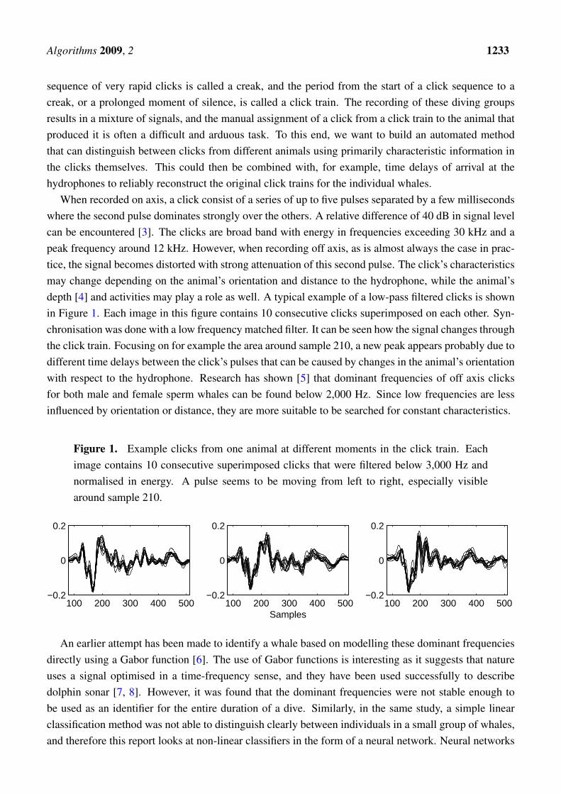
When recorded on axis, a click consist of a series of up to five pulses separated by a few millisecondswhere the second pulse dominates strongly over the others. A relative difference of 40 dB in signal levelcan be encountered [3]. The clicks are broad band with energy in frequencies exceeding 30 kHz and apeak frequency around 12 kHz. However, when recording off axis, as is almost always the case in prac-tice, the signal becomes distorted with strong attenuation of this second pulse. The click’s characteristicsmay change depending on the animal’s orientation and distance to the hydrophone, while the animal’sdepth [4] and activities may play a role as well. A typical example of a low-pass filtered clicks is shownin Figure 1. Each image in this figure contains 10 consecutive clicks superimposed on each other. Syn-chronisation was done with a low frequency matched filter. It can be seen how the signal changes throughthe click train. Focusing on for example the area around sample 210, a new peak appears probably due todifferent time delays between the click’s pulses that can be caused by changes in the animal’s orientationwith respect to the hydrophone. Research has shown [5] that dominant frequencies of off axis clicksfor both male and female sperm whales can be found below 2,000 Hz. Since low frequencies are lessinfluenced by orientation or distance, they are more suitable to be searched for constant characteristics.

Figure 1. Example clicks from one animal at different moments in the click train. Eachimage contains 10 consecutive superimposed clicks that were filtered below 3,000 Hz andnormalised in energy. A pulse seems to be moving from left to right, especially visiblearound sample 210.

100 200 300 400 500−0.2

0

0.2

100 200 300 400 500−0.2

0

0.2

Samples100 200 300 400 500

−0.2

0

0.2

An earlier attempt has been made to identify a whale based on modelling these dominant frequenciesdirectly using a Gabor function [6]. The use of Gabor functions is interesting as it suggests that natureuses a signal optimised in a time-frequency sense, and they have been used successfully to describedolphin sonar [7, 8]. However, it was found that the dominant frequencies were not stable enough tobe used as an identifier for the entire duration of a dive. Similarly, in the same study, a simple linearclassification method was not able to distinguish clearly between individuals in a small group of whales,and therefore this report looks at non-linear classifiers in the form of a neural network. Neural networks


have been used in the past for marine mammal classification with some success [9, 10]. The distributionof the characteristics from the sperm whale clicks suggested the use of a Gaussian model, and thereforea radial basis function network (RBF) architecture was used in [11] to separate sperm whales. Here, wecompare the performance of radial basis functions with support vector machines (SVM) [12, 13]. SVMuse a similar network architecture, but follow a different underlying approach and are trained differently.Training of the SVM was done in the standard approach, known as C-SVM, and a second approachknown as ν-SVM [14, 15]. An advantage of the latter method is that there is a more direct control on thenumber of support vectors used by the machine.

2. Data Acquisition, Preparation and Feature Selection

2.1. Data acquisition

The sperm whale data were collected from an inflatable boat during four field seasons spanning fourto ten weeks each (from 1997 to 1999) at Kaikoura, New Zealand [16]. Recordings were made of solitarydiving male sperm whales using an omni-directional hydrophone (Sonatech 8,178; frequencyresponse 100 Hz to 30 kHz ± 5 dB) lowered to a depth of 20 m. This hydrophone was first connected toa fixed gain amplifier (flat response from 0 to 45 kHz) and then to one channel of a Sony TCD-D10PROIIDigital Audio Tape recorder (frequency response 20 Hz to 22 kHz ± 1 dB with an anti-alias filterat 22 kHz). The recordings were digitized at 48 kHz and 16 bits. The use of data from solitary div-ing whales guarantees that no data from different animals were mixed, thus helping to obtain optimalresults. The typical duration of the recorded click trains was around 2.5 mins. The 30 mins complete divewas a sequence of such click trains. The dive was divided in 10 data segments to ease data handling andmanual analysis, but these did not exactly cover 10 click trains as the trains themselves are not alwaysvery well defined. A pause in the click production is sometimes too short to consider the continuationto be a new click train, but rather it can indicate that a few signals were not detected. Generally, a clicktrain ends with a creak where it is assumed the animal is capturing a prey, but this is not always heard ona recording as the signal can be too weak.

2.2. Data preparation and feature selection

In preparation for the classification algorithm, the clicks were manually detected, filtered for echoes,and checked for acceptable noise levels. These clicks were then denoised using a standard soft-thresholdingalgorithm, available in Wavelab [17], and synchronised using a matched filter on the low dominantfrequency with a typical example click. Initially, the data were band-pass filtered between 100 and20,000 Hz.

Data from seven different animals were available for this study, comprised of six single click trainsand a complete dive. This dive was considered to be especially interesting as it allowed to see theperformance of the algorithm, and validity of features, for the duration of an entire dive. Therefore, thedive was split up in two unequal parts. One click train early in the dive was separated and joined togetherwith the other six available click trains used for training. The remainder of the dive was put in its ownset and was only used to test the classifier, it was never used for training or parameter selection. Thisapproach simulated the situation where a classifier would have to be trained with data at the start of a


recording and allowed to assess its capacity to generalise to patterns much later in the dive sequence,that may have undergone changes as in Figure 1.

The seven click trains were used to train the classifiers. As the objective of the classification isthat a classifier can be trained with only the start of a recording and then autonomously classify theremainder, only the first 50 clicks were used from the start of each click train, which corresponds toroughly 50 seconds. The other available patterns in the click trains were used for validation, but werenever considered for training.

The features were selected using a local discriminant basis [18, 19] for the seven classes. The exactsame procedure was followed as in [6]. First, each click in the training set was expressed in a waveletpacket table. Where the usual wavelet filter retains the high-pass wavelet coefficients and continuesfiltering the low-pass scale coefficients, the wavelet packet table filters both outputs again, creating aredundant library of bases that can be selected for reconstruction of the signal (a detailed discussionabout the relationship between wavelets and filter banks can be found in [20]). With each pass throughthe wavelet filter the frequency band of the input signal is split in two, producing low and high frequencyoutputs. These outputs are stored and passed through the filter again. In this paper these recursive stepswill be called the splitting level, e.g., at level 3 the signal has been passed through the filter twice. Ata splitting level l there will be 2l−1 band limited signals, each with a bandwidth of Fs/2

l with Fs thesampling frequency. These signals will be called frequency bins (holding the energy of their respectivefrequency bands) and indexed with k. The coefficients inside each bin will be indexed by m. After thecreation of the packet table, a basis is selected that emphasises the differences between the classes. Thisdifference is measured with the help of a time-frequency energy map, defined as follows:

Γc(j, k, m) =Nc∑i

(xci(j, k, m))2/

Nc∑i

||xci ||2 (1)

where (j, k, m) denotes the position in the packet table, at splitting level j, frequency band k and co-efficient m within the bin; xc

i(j, k, m) denotes the wavelet coefficient of click sample i and class c atposition (j, k, m); xc

i the click sample i of class c; Nc the number of training samples in class c. Thismap basically sums the packet tables of the clicks within one class and allows the comparison of theenergy in a specific bin (j, k, ·) between different classes. This discrepancy can be measured with thefollowing function,

D(j, k, ·) =∑m

C−1∑p=1

C∑q=p+1

D(Γp(j, k,m), Γq(j, k, m))

Here the difference between every pair of classes is measured through an additive discriminant func-tion D, for which we used the squared l2-norm. A high value for D means that that specific bin maybe able to separate at least 2 classes that lie far apart. The local basis can now be selected using thefollowing rule, if the measure on a bin D(j, k, ·), is higher than the sum of the measures over the twobins it splits into, D(j + 1, 2k, ·) + D(j + 1, 2k + 1, ·), then it is selected, otherwise it is split. Afterthe local discriminant basis was created, we selected the 15 strongest coefficients, according to Fisher’s


discriminant given by :

FD =

∑c (sc

i −meanc(sci))

2

∑c vari(sc

i)(2)

where s are coefficients taken from a specific entry in the discriminating basis, and both the bar andvari take the mean and variance over all samples si in class c and meanc takes the mean over all classes.Essentially, this expression measures the distance between the class means and their common centrewith respect to their widths, leading to high values when samples in a class lie tightly around theirclass centre.

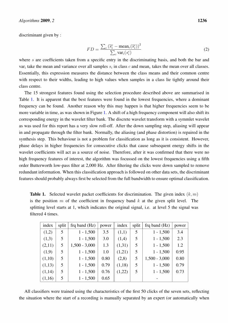
The 15 strongest features found using the selection procedure described above are summarised inTable 1. It is apparent that the best features were found in the lowest frequencies, where a dominantfrequency can be found. Another reason why this may happen is that higher frequencies seem to bemore variable in time, as was shown in Figure 1. A shift of a high frequency component will also shift itscorresponding energy in the wavelet filter bank. The discrete wavelet transform with a symmlet waveletas was used for this report has a very slow roll-off. After the down sampling step, aliasing will appearin and propagate through the filter bank. Normally, the aliasing (and phase distortion) is repaired in thesynthesis step. This behaviour is not a problem for classification as long as it is consistent. However,phase delays in higher frequencies for consecutive clicks that cause subsequent energy shifts in thewavelet coefficients will act as a source of noise. Therefore, after it was confirmed that there were nohigh frequency features of interest, the algorithm was focussed on the lowest frequencies using a fifthorder Butterworth low-pass filter at 2,000 Hz. After filtering the clicks were down sampled to removeredundant information. When this classification approach is followed on other data sets, the discriminantfeatures should probably always first be selected from the full bandwidth to ensure optimal classification.

Table 1. Selected wavelet packet coefficients for discrimination. The given index (k, m)

is the position m of the coefficient in frequency band k at the given split level. Thesplitting level starts at 1, which indicates the original signal, i.e. at level 5 the signal wasfiltered 4 times.

index split frq band (Hz) power index split frq band (Hz) power(1,2) 5 1 - 1,500 3.5 (1,1) 5 1 - 1,500 3.4(1,3) 5 1 - 1,500 3.0 (1,4) 5 1 - 1,500 2.3

(2,11) 5 1,500 - 3,000 1.3 (1,31) 5 1 - 1,500 1.2(1,9) 5 1 - 1,500 1.0 (1,21) 5 1 - 1,500 0.95

(1,10) 5 1 - 1,500 0.80 (2,8) 5 1,500 - 3,000 0.80(1,13) 5 1 - 1,500 0.79 (1,18) 5 1 - 1,500 0.79(1,14) 5 1 - 1,500 0.76 (1,22) 5 1 - 1,500 0.73(1,16) 5 1 - 1,500 0.65 -

All classifiers were trained using the characteristics of the first 50 clicks of the seven sets, reflectingthe situation where the start of a recording is manually separated by an expert (or automatically when


possible), and the remaining data would be processed automatically by the computer. The other clickswithin the sets, and the eighth set, were then used for validation.

Figure 2. Scatter plots of the four most discriminating features for five animals. Thecombination of these four characteristics already shows possible separation of five ani-mals. Moreover, the features show a strong clustering tendency that suggests the use of aGaussian model.

Feature 1

Fea

ture

2

Feature 3F

eatu

re 4

Figure 3. Variability in the two strongest features (first feature on top, second on bottom)from Table 1 during the dive.

0 200 400 600 800 1000 1200−0.5

0

0.5

Click number

Mag

nitu

de

0 200 400 600 800 1000 1200−0.5

0

0.5

Click number

Mag

nitu

de

Figure 2 shows a combination of two graphics with the four strongest features, measured usingFisher’s power of discrimination with Equation (2), from five animals that allows some insight in thefeature space. The combination of just these four features already shows some possibility of separatingthe animals. Three animals are already separated in the left figure, while two are completely mixed.Combination with the two other characteristics in the right figure allows these two to be separated aswell. An important observation in these figures, and one that we used to design the classifier, was thatthe data showed a strong clustering tendency. This suggested the application of a RBF network whichhas a natural way of modelling these clusters in its hidden layer, or a SVM which does not model theclusters themselves but their borders. Another reason we decided to use RBF and SVM based classifiersis because these methods have a local response defined by the distance of a sample to the cluster centresor support vectors. This is different from, for example, multi-layer perceptron networks, where a nodein the first layer will give the same response for all points on a specific hyperplane. Although, as a result,perceptron networks may have better generalisation in areas of the feature space that are poorly sampled,


we preferred the local properties that allowed more accurate modelling of the feature space as it is pre-sented in Figure 2. To have an idea about the variability of the features, Figure 3 shows the two strongestfeatures during the whole dive. From this figure it can be suspected that 50 consecutive samples may notalways be sufficient to characterise the variance of the feature.

3. Classification Description

3.1. Radial basis function network

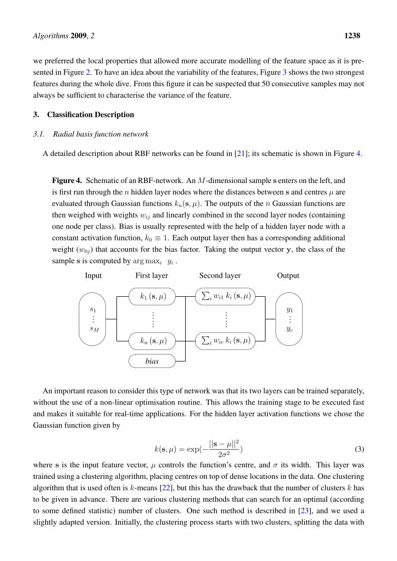
A detailed description about RBF networks can be found in [21]; its schematic is shown in Figure 4.

Figure 4. Schematic of an RBF-network. An M -dimensional sample s enters on the left, andis first run through the n hidden layer nodes where the distances between s and centres µ areevaluated through Gaussian functions kn(s, µ). The outputs of the n Gaussian functions arethen weighed with weights wij and linearly combined in the second layer nodes (containingone node per class). Bias is usually represented with the help of a hidden layer node with aconstant activation function, k0 ≡ 1. Each output layer then has a corresponding additionalweight (w0j) that accounts for the bias factor. Taking the output vector y, the class of thesample s is computed by arg maxi yi .

Input

'

&

$

%

s1...sM

First layerº

¹

·

¸......º

¹

·

¸¶µ

³´

k1 (s, µ)

kn (s, µ)

bias

Second layerº

¹

·

¸......º

¹

·

¸

∑i wi1 ki (s, µ)

∑i wic ki (s, µ)

Output

'

&

$

%

y1...yc

An important reason to consider this type of network was that its two layers can be trained separately,without the use of a non-linear optimisation routine. This allows the training stage to be executed fastand makes it suitable for real-time applications. For the hidden layer activation functions we chose theGaussian function given by

k(s, µ) = exp(−||s− µ||22σ2

) (3)

where s is the input feature vector, µ controls the function’s centre, and σ its width. This layer wastrained using a clustering algorithm, placing centres on top of dense locations in the data. One clusteringalgorithm that is used often is k-means [22], but this has the drawback that the number of clusters k hasto be given in advance. There are various clustering methods that can search for an optimal (accordingto some defined statistic) number of clusters. One such method is described in [23], and we used aslightly adapted version. Initially, the clustering process starts with two clusters, splitting the data with


k-means. A cluster was accepted and removed from the feature space when its projection in the directionof its principal component resembled a normal distribution, where normality was measured using theAnderson-Darling statistic [24, 25]. The value for k was then adjusted for the removed clusters andincreased by one. The remaining clusters were combined and clustered again. This process was repeateduntil all clusters were accepted. To prevent random outcomes, k-means was always initialised by placingan additional centre in a cluster on the feature vector furthest away from the data’s centre [26]. In orderto take advantage of class information in the clustering process, the clustering was done on the individualclasses, instead of on all the data as a whole.

Once the first layer has been defined by the clusters, training of the second layer is trivial; the numberof nodes was set to the number of classes, using binary encoding for the targets (e.g., a sample from class1 has target [1 0 0]t, and a sample from class 3 has target [0 0 1]t). Calculation of the weights, using asum-of-squares error function, is then a fast linear process [21].

3.2. Support vector machine classification

Another popular network model that uses Gaussian functions are support vector machines (SVM).SVM generally solve the two class problem with a network structure that is similar to the RBF structurein Figure 4. Since there are only two classes, SVM only have one output. The main difference betweenthe two networks relies on the underlying approach and in the way they are trained. Where the RBFnetwork places Gaussian kernels on the cluster centres formed by the features in the feature space,the SVM network places the Gaussian kernels on those samples that define the boundary between twoclasses. These points are found by creating a separating hyperplane inside a higher dimensional featurespace. A reason to consider SVM is that they tend to show strong generalisation performance [22]. In thecase of SVM, the interpretation of the first layer is that it projects the data to a feature space where thetwo classes can be separated by a hyperplane. The position of the hyperplane is decided by those pointsthat lie within a certain margin between the two classes (the support vectors). The projected feature spaceis allowed (or preferred) to have a higher dimension, as there is no penalty in the form of computationaldrawbacks or the ’curse of dimensionality’ since the actual mapping is never performed. All necessarycalculations in the projected feature space are evaluated through inner products, which can be done witha kernel function. In our case this was the Gaussian function (3) that was also used for the RBF network.

The training stage for SVM both defines the number of nodes in the hidden layer and calculates theoutput layer weights at the same time. There several approaches to train the network in the case ofnon-separable classes. First we looked at C-SVM, which aims at solving the following optimisationproblem [27]:

minw,ξ,b

||w||2 + C

N∑i=1

ξi (4)

under the constraint that the training data should classify correctly, and where w is the direction of thenormal vector on the separating plane, N the number of samples, ξ are the slack vectors which are non-zero for the samples that lie within the margin, and C is the pre-defined penalty on these points. Thisproblem has a straightforward optimal solution wo using Lagrange multipliers [27], expressed as follows


wo =N∑

i=1

αitiφ(si) (5)

where ti are the targets of mapped inputs si. Only a few of the Lagrange multipliers αi will be non-zero,and those define both the first layer support vectors (si) and the second layer weights. It should be notedthat wo is never actually evaluated as the classification function given by

f(s) = wTo φ(s) + bo =

∑i ∈ sv

αitiφ(si) · φ(s) + bo (6)

evaluates the inner product directly though the kernel function.A second training method that trains a SVM network regulating classification errors is ν-SVM [15].

The optimisation problem that is solved is then given by

minw,ξ,b,ρ

1

2||w||2 − νρ +

1

N

N∑i=1

ξi (7)

under the constraint of correct classification, and where ρ is the margin in the mapped feature space andis left as a free variable. The fixed constant ν gives some control over both the error rate on the trainingset (Pe, the ratio between misclassifications and number of training patterns) and the number of supportvectors (Ns) from the optimisation through the relationships [22] :

Pe ≤ ν; and Nν ≤ Ns. (8)

This can be a useful property as the number of support vectors play a large role on the speed ofthe network.

The SVM network only separates two classes, but the same algorithm can easily be extended to severalclasses, for example by using a one-against-one approach. For this classification method a separatemachine is created for every combination of two classes, meaning that when there are n classes thisresults in n(n−1)

2machines. A new pattern is then presented to all the machines, and the class that occurs

most frequently in the outcome is chosen. In the case when there are two or more classes with identicalfrequencies, the pattern is defined as unclassifiable.

4. Classification Results

In order to classify the patterns, the 15 strongest features according to equation (2) were selectedfrom the local discriminant basis. The C-SVM results were obtained using a toolbox from [28]; customcode in Matlab was written to obtain the ν-SVM results. For both SVM approaches a total numberof 21 support vector machines was used to classify the seven classes; every support vector machine wastrained with 100 patterns. Each machine has two parameters that can be tuned, the width and either theparameter C or ν. To simplify the training stage, their values were kept identical over all machines. Inorder to select suitable parameters, the machines were trained while varying one parameter and keepingthe other one fixed. At each value the classifier was trained 10 times with noise added to the data.The noise was drawn from a zero-mean normal distribution with the standard deviation taken from thestandard deviation of the features.


Parameter selection for C-SVM is shown in Figure 5. The values were based on the second set whichproved more problematic than the others. On the left side the error penalty C is varied between 0.1 to2. The top left graph shows the true positive and false positive rates. In order to create these values,all other classes were combined into the negative class. It has to be kept in mind that the classifierwas not especially trained to improve performance on this set, which means that for some parameters theclassifier as a whole might have had better performance, while set 2 performed worse. Bottom left showsthe total number of support vector machines that were used for each C. As can be seen, a low penaltyallowed many patterns to reside inside the margin, leading to many support vectors, while increasing thepenalty discouraged this. On the right side variation of the kernel width is shown. In this case, a narrowwidth did not cover the feature space very well, and many support vectors were used (the maximum totalnumber of support vectors that could be used were 21× 100 for 21 machines with 100 training patternseach), increasing the width and coverage in feature space required less vectors. A high true positive ratewas often combined with a high number of support vectors. A reasonable value for C would be around1.0 and for the width around 0.30.

Figure 5. Performance of the C-svm classifier on problem set 6. The top row images plotthe false positive rate (FPR) versus the true positive rate (TPR). On the left the regularisationparameter C is varied between the values on the colour bar with fixed kernel width σ = 0.30.The right image varies the kernel width between the values on the colour bar with fixedC = 1.1.

2 3 4 5 665

70

75

FPR (%)

TP

R (

%)

0.5

1

1.5

2

0.5 1 1.5 2500

1000

C

# S

V

3 4 5 665

70

75

FPR (%)

TP

R (

%)

0.1

0.2

0.3

0.4

0.1 0.2 0.3 0.4500

2000

σ

# S

V

In the case of ν-SVM similar figures were made to decide on reasonable parameter values inFigure 6. The affect of varying ν is seen on the left side, in this case increasing ν (and thus increas-ing the width of the margin) will also increase the lower bound given in Equation (8) leading to a highernumber of support vectors. Here, a narrow margin was preferred with ν around 0.13 and σ around 0.25.

The left side of Table 2 shows the complete classification results using C-SVM with σ = 0.30 andC = 1.1. The machines used 337 support vectors in total, 141 of which were unique (training patternsfrom one class can be used by multiple machines). The classification values are the percentages ofcorrectly classified clicks. The undecided row contains the percentages of patterns that could not beclassified by the voting mechanism of the SVM classifiers. The generalisation to the validation set is


quite good except for the second set. In particular, the eighth set classifies very well. Analysing theerrors in this set showed that there was one particular noisy time period during which many clicks weremisclassified. Removing this period left 993 clicks, 82% of which were correctly classified. In this casethe percentage of undecided patterns was somewhat high for a few data sets. Perhaps combining theinformation from the SVM in a different, more sophisticated, way may lead to improved results.

Figure 6. As in Figure 5, but with the ν-svm classifier. On the left the regularisationparameter ν is varied between the values on the colour bar with fixed kernel width σ = 0.24.The right image varies the kernel width between the values on the colour bar with fixedν = 0.13.

4 4.5 5 5.565

70

75

FPR (%)

TP

R (

%)

0.1

0.2

0.3

0 0.1 0.2 0.3500

1000

ν

# S

V

3 3.5 4 4.5 5 5.540

60

80

FPR (%)

TP

R (

%)

0.1

0.2

0.3

0.4

0.1 0.2 0.3 0.4500

2000

σ

# S

V

In the centre of Table 2 the results are shown when using ν-SVM. While ν gave good control over thenumber of support vectors in use, it did not lead to both a low number and good performance. For givenparameters the algorithm used 464 SV (of which 153 were unique), with roughly the same performanceas C-SVM. Especially the generalisation in set 8 had somewhat improved. In this case, removing thenoisy segment improved classification of set 8 to 84%. The number of undecided samples was lowerthan for C-SVM, but it may still be worth to look for a better way to combine machines in order tohandle multiple classes.

The radial basis function method also had two parameters that could be tuned. In our case, theclustering algorithm determined the number of nodes in the hidden layer, leaving only the widths to beadjusted, which were again set identical for all Gaussian kernels. Clustering led to a total of 15 clusters,or nodes in the hidden layer (plus the additional bias node). The use of this clustering algorithm, insteadof trying k-means for different values of k, gave better results on these data, while using less centres.Figure 7 shows the effect of varying the width with the fixed number of hidden nodes on set two. Tominimise the false positives, a value over 0.15 seems adequate.

The complete classification results with the RBF network are shown in the most right part of Table2. The width was set to 0.34 with 15 hidden nodes. Classification of the validation set was comparableto SVM, although generalisation to the entire dive was slightly worse. Removal of the noisy data seg-ment in the eighth set led to 79% correct classification, compared to the 82% and 84% that were foundwith SVM.


Table 2. Classification results using the different classifiers. The left and centre of thetable shows the outcome using C-SVM and ν-SVM, the right side the outcome using RBF.It can be seen that both SVM approaches generalise slightly better towards unknown data atthe cost of using more information, as under given parameters the SVM used 337 and 464support vectors respectively, while RBF used only 15 centres. The last row are the undecidedpatterns for the SVM classifiers.

C-SVM σ = 0.30 C = 1.1 ν-SVM σ = 0.24 ν = 0.15 RBF σ = 0.34

Set 1 2 3 4 5 6 7 8 1 2 3 4 5 6 7 8 1 2 3 4 5 6 7 8

1 83 5 12 3 0 0 0 4 78 5 12 3 0 0 0 3 86 5 6 3 0 4 0 6

2 8 66 0 0 0 0 1 6 9 69 0 0 0 0 1 6 3 67 0 0 0 0 2 7

3 1 0 79 1 0 0 0 2 3 0 79 1 1 0 0 2 9 3 91 1 1 2 1 5

4 0 0 0 80 1 0 0 1 0 0 0 85 3 0 0 1 0 0 0 92 3 0 0 1

5 0 2 3 15 97 0 0 3 0 2 3 10 96 0 0 1 1 8 3 3 96 0 2 2

6 1 13 3 1 0 100 1 8 1 13 3 1 0 100 1 8 1 8 0 0 0 87 1 7

7 5 9 0 1 0 0 98 73 8 8 0 1 0 0 98 79 1 9 0 1 0 7 94 72

und 2 5 3 0 1 0 0 3 2 2 3 0 0 0 0 1

Figure 7. Classification performance on set two using RBF. The kernel width was variedalong values of the colour bar.

0 1 2 3 4 5 6 755

60

65

FPR (%)

TP

R (

%)

0.10.20.3

Comparing the results of the classifiers in Table 2, there are considerable differences in performanceon for example class 3 between SVM and RBF, but most validation sets, except the long dive, wereclassified better. It suggests that the data were better described by their class centres than their bound-aries. It could be that to cover the variability in the features the margins in the SVM need to be widened.However, this also greatly increased the number of support vectors as shown in Figures 5 and 6 whichis undesirable. More full dives need to be collected to understand the variability in the features andto determine which of the two approaches, class centres or class boundaries, will perform better. Thepoor performance of all classifiers on the second class could be caused by a drop in the signal to noiseratio towards the end of the click train, perhaps combined with changes in the orientation of the ani-mal. It should be noted that when the training set of 50 clicks was created with random draws from thewhole click train, all classifiers performed considerably better on this set (SVM could reach 98% correct,


RBF 88%, without attempting to further optimise these numbers). While this is not directly useful in apractical situation, it does show the capability of the classifiers.

The RBF network took very little time to be trained and classify all available data, an average of only 2seconds was needed. In contrast, the ν-SVM trained and classified all data in 10 seconds, while C-SVMtook 15 (our configuration consisted of 32-bit Matlab running on an AMD 64 X2 4200+ with 2 GB RAM;just a single core was used by Matlab). These timings should only be considered as a rough indication ofthe speed differences between the algorithms, as the code was not especially optimised for Matlab. Forexample, initially C-SVM took 43 seconds to execute, but vectorizing a critical loop took off almost halfa minute. The times do indicate that real-time execution is possible. An optimised C implementation willlikely bring the performances closer together, but the SVM algorithms will still remain slower simplybecause they use more information (support vectors) and the optimisation routines in the learning phasetake more time than the clustering routine for RBF. Since the RBF network contained considerablyless information and executed faster than the SVM, RBF could be, based on these data, considered toperform better.

5. Conclusion

We showed that separation of sperm whale sonar clicks using a Gaussian kernel with support vectormachines, or radial basis functions, has the potential to work well on single click trains. It is not yetclear if the features are constant enough to allow their use during an entire dive. While we found goodperformance on the single dive we had available, this may not be the case when this type of data is avail-able from all whales. It also has to be kept in mind that these data came from individually diving whales,and not from a group. Unfortunately, we did not have group data available that allowed separation ofthe individual animals with certainty. If the features evolve during the dive then it may be necessary tolook for a method that can adapt itself to these gradual changes. In the case of SVM, drawbacks forreal-time usage may be the use of optimisation routines for learning, as well as the amount of neces-sary support vectors and the number of machines which slow down its execution. On the other hand,radial basis function classification required less information to obtain similar results and its fast trainingstage may allow it to adapt more easily to a changing environment. However, it showed slightly worsegeneralisation capacity.

An important detail of the proposed classification methods is that they have to be trained with alreadyseparated training data. This is not necessarily a problem when classification is done off-line and thetraining sets can be manually selected, but when used in real-time this part needs to be done automaticallyas well. This would require at least an estimate of the number of animals diving at that instant, whichcould be done with unsupervised clustering methods. Results to this end were obtained by [29], usingspectral clustering on the first two cepstral coefficients and the slope of the onset of a click. Anotherstudy [30] used a self organising map to cluster data using sperm whale codas. While these are neveremitted during a foraging dive, a similar technique might be applicable on regular clicks.

The classification process itself could be improved in various ways. The local discriminant basisis selected on the requirement that it can reconstruct a signal. However, we are not interested in thereconstructed signal, and therefore we can use a much wider range of wavelets (e.g., non-orthogonal)and different time-frequency bin selection procedures. Other issues are the synchronisation of the clicks,


which generally presented a small error that can affect the wavelet coefficients, and the selection of thecharacteristics. The strongest features are now chosen with Fisher’s discriminant, but the classificationitself is based on non-linear dependencies between the features. A similar non-linear measure for thefeature strength might result in a better selection.

It is possible that other data sets cannot use the same local basis. Different noise patterns and environ-ments may lead to a different LDB selection. Even when the basis is the same, the strongest coefficientsmay not be the same as ones selected in this study. Therefore, it is probably not possible to define afixed basis with features that can be universally applied, and these will have to be re-evaluated for everyrecording. More data will also be necessary to gain better insights into the variability of the click featuresduring an entire dive, and especially to investigate the possibility of using similar algorithms for uniqueidentification of an animal at different times and in different environments.

Acknowledgements

The authors want to thank Natalie Jaquet for providing the recordings. This study was funded by theBBVA (Banco Bilbao Vizcaya Argentaria) Foundation.

References

1. Whitehead, H. Sperm Whales: Social Evolution in the Ocean, 1st Ed.; University Of Chicago Press:Chicago, IL, USA, 2003; pp. 79-81.

2. Miller, P.; Johnson, M.; Tyack, P. Sperm whale behaviour indicates the use of echolocation clickbuzzes ’creaks’ in prey capture. Proc. R. Soc. Lond. B Biol. Sci. 2004, 271, 2239-2247.

3. Møhl, B.; Wahlberg, M.; Madsen, P.; Heerfordt, A.; Lund, A. The monopulsed nature of spermwhale clicks. J. Acoust. Soc. Am. 2003, 114, 1143-1154.

4. Thode, A.; Mellinger, D.; Stienessen, S.; Martinez, A.; Mullin, K. Depth-dependent acoustic fea-tures of diving sperm whales (Physeter macrocephalus) in the Gulf of Mexico. J. Acoust. Soc. Am.2002, 112, 308-321.

5. Goold, J.; Jones, S. Time and frequency domain characteristics of sperm whale clicks. J. Acoust.Soc. Am. 1995, 98, 1279-1291.

6. van der Schaar, M.; Delory, E.; van der Weide, J.; Kamminga, C.; Goold, J.; Jaquet, N.; Andre,M. A comparison of model and non-model based time-frequency transforms for sperm whale clickclassification. J. Mar. Biol. Assoc. 2007, 87, 27-34.

7. Kamminga, C.; Cohen Stuart, A. Wave shape estimation of delphinid sonar signals, a parametricmodel approach. Acoust. Lett. 1995, 19, 70-76.

8. Kamminga, C.; Cohen Stuart, A. Parametric modelling of polycyclic dolphin sonar wave shapes.Acoust. Lett. 1996, 19, 237-244.

9. Huynh, Q.; Cooper, L.; Intrator, N.; Shouval, H. Classification of underwater mammals usingfeature extraction based on time-frequency analysis and BCM theory. IEEE T. Signal Proces. 1998,46, 1202-1207.

10. Murray, S.; Mercado, E.; Roitblat, H. The neural network classification of false killer whale (Pseu-dorca crassidens) vocalizations. J. Acoust. Soc. Am. 1998, 104, 3626-3633.


11. van der Schaar, M.; Delory, E.; Catala, A.; Andre, M. Neural network based sperm whale clickclassification. J. Mar. Biol. Assoc. 2007, 87, 35-38.

12. Scholkopf, B.; Sung, K.K.; Burges, C.; Girosi, F.; Niyogi, P.; Poggio, T.; Vapnik, V. Comparingsupport vector machines with gaussian kernels to radial basis function classifiers. IEEE T. SignalProces. 1997, 45, 2758-2765.

13. Debnath, R.; Takahashi, H. Learning Capability: Classical RBF Network vs. SVM with GaussianKernel. In Proceedings of Developments in Applied Artificial Intelligence: 15th International Con-ference on Industrial and Engineering. Applications of Artificial Intelligence and Expert Systems,IEA/AIE 2002, Cairns, Australia, June 17-20, 2002; Vol. 2358.

14. Scholkopf, B.; Smola, A.; Williamson, R.; Bartlett, P. New support vector algorithms. NeuralComput. 2000, 12, 1207-1245.

15. Chen, P.; Lin, C.; Scholkopf, B. A Tutorial on ν-Support Vector Machines. 2003; Available online:http://www.csie.ntu.edu.tw/˜cjlin/papers/nusvmtutorial.pdf, accessed April 12, 2007.

16. Jaquet, N.; Dawson, S.; Douglas, L. Vocal behavior of male sperm whales: Why do they click? J.Acoust. Soc. Am. 2001, 109, 2254-2259.

17. Donoho, D.; Duncan, M.; Huo, X.; Levi, O. Wavelab 850. 2007; Available online: ˜wavelab/,accessed September 28, 2007.

18. Saito, N.; Coifman, R. Local discriminant bases. In Proceedings of Mathematical Imaging: WaveletApplications in Signal and Image Processing II, San Diego, CA, USA, July 27-29, 1994; Vol. 2303.

19. Delory, E.; Potter, J.; Miller, C.; Chiu, C.-S. Detection of blue whales A and B calls in the northeastPacific Ocean using a multi-scale discriminant operator. In Proceedings of the 13th Biennial Con-ference on the Biology of Marine Mammals,b Maui, Hawaii, USA, 1999; published on CD-ROM(arl.nus.edu.sg).

20. Strang, G.; Nguyen, T. Wavelets and Filter Banks. Wellesley-Cambridge: Wellesley, MA, USA,1997.

21. Bishop, C. Neural Networks for Pattern Recognition; Oxford University: Oxford, UK, 1995.22. Theodoridis, S.; Koutroumbas, K. Pattern Recognition, 3rd Ed.; Academic Press: Maryland

Heights, MO, USA, 2006.23. Hamerly, G.; Elkan, C. Learning the k in k-means. In Proceedings of the 17th Annual Conference

on Neural Information Processing Systems (NIPS), Vancouver, Canada, December 2003.24. D’Agostino, R.; Stephens, M. Goodness-Of-Fit Techniques (Statistics, a Series of Textbooks and

Monographs). Marcel Dekker: New York, NY, USA, 1986.25. Romeu, J. Anderson-Darling: A Goodness of Fit Test for Small Samples Assumptions; Technical

Report 3; RAC START, 2003.26. Katsavounidis, I.; Kuo, C.; Zhang, Z. A new initialization technique for generalized lloyd iteration.

IEEE Signal Proc. Let. 1994, 1, 144-146.27. Cortes, C.; Vapnik, V. Support-vector networks. Mach. Learn. 1995, 20, 273-297.28. Gunn, S. Matlab Support Vector Machine Toolbox; 2001; Available online: http://www.isis.ecs.soton.

ac.uk/resources/svminfo/, accessed September 27, 2006.


29. Halkias, X.; Ellis, D. Estimating the number of marine mammals using recordings from one mi-crophone. In Proceedings of the IEEE International Conference on Acoustics, Speech, and SignalProcessing ICASSP-06, Toulouse, France, May 14-19, 2006.

30. Ioup, J.; Ioup, G. Self-organizing maps for sperm whale identification. In Proceedings ot Twenty-Third Gulf of Mexico Information Transfer Meeting; McKay, M., Nides, J., Eds.; U.S. Depart-ment of the Interior, Minerals Management Service: New Orleans, LA, USA, January 11, 2005;pp. 121-129.

c© 2009 by the authors; licensee Molecular Diversity Preservation International, Basel, Switzerland.This article is an open-access article distributed under the terms and conditions of the Creative CommonsAttribution license http://creativecommons.org/licenses/by/3.0/.

Classification of Sperm Whale Clicks (Physeter ...

Documents

Transcript of Classification of Sperm Whale Clicks (Physeter ...