Classification of patterns of EEG synchronization for ...nin/Courses/Seminar14a/Epilepsy.pdf ·...
14
Classification of patterns of EEG synchronization for seizure prediction q Piotr Mirowski a, * , Deepak Madhavan b , Yann LeCun a , Ruben Kuzniecky c a Courant Institute of Mathematical Sciences, New York University, 719 Broadway, New York, NY 10003, USA b Department of Neurological Sciences, 982045 University of Nebraska Medical Center, Omaha, NE 68198, USA c New York University Comprehensive Epilepsy Center, 223 East 34th St., New York, NY 10016, USA article info Article history: Accepted 2 September 2009 Available online 17 October 2009 Keywords: Seizure prediction Feature extraction Classification Pattern recognition Machine learning Neural networks abstract Objective: Research in seizure prediction from intracranial EEG has highlighted the usefulness of bivariate measures of brainwave synchronization. Spatio-temporal bivariate features are very high-dimensional and cannot be analyzed with conventional statistical methods. Hence, we propose state-of-the-art machine learning methods that handle high-dimensional inputs. Methods: We computed bivariate features of EEG synchronization (cross-correlation, nonlinear interde- pendence, dynamical entrainment or wavelet synchrony) on the 21-patient Freiburg dataset. Features from all channel pairs and frequencies were aggregated over consecutive time points, to form patterns. Patient-specific machine learning-based classifiers (support vector machines, logistic regression or con- volutional neural networks) were trained to discriminate interictal from preictal patterns of features. In this explorative study, we evaluated out-of-sample seizure prediction performance, and compared each combination of feature type and classifier. Results: Among the evaluated methods, convolutional networks combined with wavelet coherence suc- cessfully predicted all out-of-sample seizures, without false alarms, on 15 patients, yielding 71% sensitiv- ity and 0 false positives. Conclusions: Our best machine learning technique applied to spatio-temporal patterns of EEG synchroni- zation outperformed previous seizure prediction methods on the Freiburg dataset. Significance: By learning spatio-temporal dynamics of EEG synchronization, pattern recognition could capture patient-specific seizure precursors. Further investigation on additional datasets should include the seizure prediction horizon. Ó 2009 International Federation of Clinical Neurophysiology. Published by Elsevier Ireland Ltd. All rights reserved. 1. Introduction Recent multi-center clinical studies showed evidence of pre- monitory symptoms in 6.2% of 500 patients with epilepsy (Schu- lze-Bonhage et al., 2006). Another interview-based study found that 50% of 562 patients felt ‘‘auras” before seizures (Rajna et al., 1997). Such clinical observations give an incentive to search for premonitory changes on EEG recordings from the brain, and to implement a device that would automatically forewarn the pa- tient. However, and despite decades of research, research in sei- zure prediction is still qualified as a ‘‘long and winding road” (Mormann et al., 2007). Most current seizure prediction approaches (Arnhold et al., 1999; Iasemidis et al., 2005; Lehnertz and Litt, 2005; Lehnertz et al., 2007; Le Van Quyen et al., 2005; Litt and Echauz, 2002; Mor- mann et al., 2006, 2007) can be summarized into (1) extracting measurements from EEG over time and (2) classifying them into a preictal or interictal state. The ictal and postictal states are dis- carded from the classification, because the task is not to detect undergoing seizures, but eventually to warn the patient about fu- ture ones, so that the patient, the clinician, or an implanted device can act accordingly. The method described in this article follows a similar method- ology: (1) feature extraction, followed by (2) binary classification of patterns of features into preictal or interictal states. Section 1.1 of the Introduction overviews existing techniques for feature extraction from EEG (1), while Section 2.2 and Appendix A detail specific features used in the proposed method. The breakthrough of our technique lies in the pattern recogni- tion and machine learning-powered classification of features (2). The proposed pattern-based classification is described in Sections 2.3 through 2.5. As can be seen in Section 1.2, the proposed method 1388-2457/$36.00 Ó 2009 International Federation of Clinical Neurophysiology. Published by Elsevier Ireland Ltd. All rights reserved. doi:10.1016/j.clinph.2009.09.002 q Portions of this manuscript were presented at the 2008 American Epilepsy Society annual meeting and at the 2008 IEEE Workshop on Machine Learning for Signal Processing. * Corresponding Author. Address: Courant Institute of Mathematical Sciences, New York University, 719 Broadway, 12th Floor, New York, NY 10003, USA. Tel.: +1 203 278 1803; fax: +1 212 263 8342. E-mail address: [email protected] (P. Mirowski). Clinical Neurophysiology 120 (2009) 1927–1940 Contents lists available at ScienceDirect Clinical Neurophysiology journal homepage: www.elsevier.com/locate/clinph
Transcript of Classification of patterns of EEG synchronization for ...nin/Courses/Seminar14a/Epilepsy.pdf ·...
Clinical Neurophysiology 120 (2009) 1927–1940
Contents lists available at ScienceDirect
Clinical Neurophysiology
journal homepage: www.elsevier .com/locate /c l inph
Classification of patterns of EEG synchronization for seizure prediction q
Piotr Mirowski a,*, Deepak Madhavan b, Yann LeCun a, Ruben Kuzniecky c
a Courant Institute of Mathematical Sciences, New York University, 719 Broadway, New York, NY 10003, USAb Department of Neurological Sciences, 982045 University of Nebraska Medical Center, Omaha, NE 68198, USAc New York University Comprehensive Epilepsy Center, 223 East 34th St., New York, NY 10016, USA
a r t i c l e i n f o
Article history:Accepted 2 September 2009Available online 17 October 2009
Keywords:Seizure predictionFeature extractionClassificationPattern recognitionMachine learningNeural networks
1388-2457/$36.00 � 2009 International Federation odoi:10.1016/j.clinph.2009.09.002
q Portions of this manuscript were presented atSociety annual meeting and at the 2008 IEEE WorkshSignal Processing.
* Corresponding Author. Address: Courant InstitutNew York University, 719 Broadway, 12th Floor, New203 278 1803; fax: +1 212 263 8342.
E-mail address: [email protected] (P. M
a b s t r a c t
Objective: Research in seizure prediction from intracranial EEG has highlighted the usefulness of bivariatemeasures of brainwave synchronization. Spatio-temporal bivariate features are very high-dimensionaland cannot be analyzed with conventional statistical methods. Hence, we propose state-of-the-artmachine learning methods that handle high-dimensional inputs.Methods: We computed bivariate features of EEG synchronization (cross-correlation, nonlinear interde-pendence, dynamical entrainment or wavelet synchrony) on the 21-patient Freiburg dataset. Featuresfrom all channel pairs and frequencies were aggregated over consecutive time points, to form patterns.Patient-specific machine learning-based classifiers (support vector machines, logistic regression or con-volutional neural networks) were trained to discriminate interictal from preictal patterns of features. Inthis explorative study, we evaluated out-of-sample seizure prediction performance, and compared eachcombination of feature type and classifier.Results: Among the evaluated methods, convolutional networks combined with wavelet coherence suc-cessfully predicted all out-of-sample seizures, without false alarms, on 15 patients, yielding 71% sensitiv-ity and 0 false positives.Conclusions: Our best machine learning technique applied to spatio-temporal patterns of EEG synchroni-zation outperformed previous seizure prediction methods on the Freiburg dataset.Significance: By learning spatio-temporal dynamics of EEG synchronization, pattern recognition couldcapture patient-specific seizure precursors. Further investigation on additional datasets should includethe seizure prediction horizon.� 2009 International Federation of Clinical Neurophysiology. Published by Elsevier Ireland Ltd. All rights
reserved.
1. Introduction
Recent multi-center clinical studies showed evidence of pre-monitory symptoms in 6.2% of 500 patients with epilepsy (Schu-lze-Bonhage et al., 2006). Another interview-based study foundthat 50% of 562 patients felt ‘‘auras” before seizures (Rajna et al.,1997). Such clinical observations give an incentive to search forpremonitory changes on EEG recordings from the brain, and toimplement a device that would automatically forewarn the pa-tient. However, and despite decades of research, research in sei-zure prediction is still qualified as a ‘‘long and winding road”(Mormann et al., 2007).
f Clinical Neurophysiology. Publish
the 2008 American Epilepsyop on Machine Learning for
e of Mathematical Sciences,York, NY 10003, USA. Tel.: +1
irowski).
Most current seizure prediction approaches (Arnhold et al.,1999; Iasemidis et al., 2005; Lehnertz and Litt, 2005; Lehnertzet al., 2007; Le Van Quyen et al., 2005; Litt and Echauz, 2002; Mor-mann et al., 2006, 2007) can be summarized into (1) extractingmeasurements from EEG over time and (2) classifying them intoa preictal or interictal state. The ictal and postictal states are dis-carded from the classification, because the task is not to detectundergoing seizures, but eventually to warn the patient about fu-ture ones, so that the patient, the clinician, or an implanted devicecan act accordingly.
The method described in this article follows a similar method-ology: (1) feature extraction, followed by (2) binary classificationof patterns of features into preictal or interictal states. Section1.1 of the Introduction overviews existing techniques for featureextraction from EEG (1), while Section 2.2 and Appendix A detailspecific features used in the proposed method.
The breakthrough of our technique lies in the pattern recogni-tion and machine learning-powered classification of features (2).The proposed pattern-based classification is described in Sections2.3 through 2.5. As can be seen in Section 1.2, the proposed method
ed by Elsevier Ireland Ltd. All rights reserved.
1928 P. Mirowski et al. / Clinical Neurophysiology 120 (2009) 1927–1940
takes advantage of decade of research in image processing and vi-sion, but is also a novelty in the field of seizure prediction. More-over, Section 3 shows that our method achieves superior seizureprediction results on the Freiburg EEG dataset (described in Section2.1). Finally, Section 4 discusses the limitations of the proposedmethod.
1.1. Feature extraction from EEG
Seizure prediction methods have in common an initial buildingblock consisting of the extraction of EEG features. All EEG featuresare computed over a short time window of a few seconds to a fewminutes. One can distinguish between univariate measures, com-puted on each EEG channel separately, and bivariate (or multivar-iate) measures, which quantify some relationship, such assynchronization, between two or more EEG channels. Although aplethora of univariate features has been investigated for seizureprediction (Esteller et al., 2005; Harrison et al., 2005; Jerger et al.,2005; Jouny et al., 2005), none of them has succeeded in that task,as illustrated in an extensive study comparing most univariate andbivariate techniques (Mormann et al., 2005), which also confirmedthe superiority of bivariate measurements for seizure prediction.
In parallel to comparative study (Mormann et al., 2005), and de-spite the current lack of a complete neurological understanding ofthe preictal brain state, researchers increasingly hypothesize thatbrainwave synchronization patterns might differentiate interictal,preictal and ictal states (Le Van Quyen et al., 2003). From clinicalobservations on the synchronization of neural activity, it has beensuggested that interictal phases correspond to moderate synchro-nization within the brain at large frequency bands, and that thereis a preictal decrease in the beta range synchronization betweenthe epileptic focus and other brain areas, followed by a subsequenthyper-synchronization at the seizure onset. These considerationsmotivated our choice of bivariate EEG features.
As described in Section 2.2 and Appendix A, this article evalu-ates four kinds of EEG synchronization (bivariate) features: onesimple linear feature called Maximum Cross-Correlation (Mor-mann et al., 2005; Appendix A.1) and three nonlinear features.The first and popular nonlinear measure is Nonlinear Interdepen-dence, which measures the distance, in state-space, betweentime-delay embedded trajectories of two EEG channels (Arnholdet al., 1999; Mormann et al., 2005) (see Appendix A.2). The secondmeasure, also called Dynamical Entrainment, is based on the mea-sure of chaos in the EEG. It estimates from any two observed timeseries, the difference of their largest Lyapunov exponents, i.e. theexponential rates of growth of an initial perturbation (see Appen-dix A.3). Finally, a third type of nonlinear bivariate measures thattakes advantage of the frequency content of EEG signals is phasesynchronization. First, two equivalent techniques can be employedto extract the frequency-specific phase of EEG signal: band-pass fil-tering followed by Hilbert transform or Wavelet transform (Le VanQuyen et al., 2001). Then, statistics on the difference of phases be-tween two channels (such as phase-locking synchrony) are com-puted for specific combinations of channels and frequencies (LeVan Quyen et al., 2005).
1.2. Feature classification for seizure prediction
Once univariate or bivariate, linear or nonlinear measurementsare derived from EEG, the most common approach for seizure pre-diction is the simple binary classification of a single variable (Lehn-ertz et al., 2007; Mormann et al., 2005). Their hypothesis is thatthere should be a preictal increase or decrease in the values of anEEG-derived feature. Statistical methods consist in an a-posterioriand in-sample tuning of a binary classification threshold (e.g.pre-ictal vs. interictal) on that unique measure extracted from EEG.
The usage of a simple binary threshold has limitations detailedin Section 4.2. Essentially, it does not allow using high-dimensionalfeatures. By contrast, machine learning theory (sometimes alsocalled statistical learning theory) easily handles high-dimensionaland spatio-temporal data, as illustrated in its countless applica-tions such as video or sound recognition.
Most importantly, machine learning provides both with a meth-odology for learning by example from data, and for quantifying theefficiency of the learning process (Vapnik, 1995). The available dataset is divided into a training set (‘‘in-sample”) and a testing set(‘‘out-of-sample”). Training consists in iteratively adjusting theparameters of the machine in order to minimize the empirical er-ror made on in-sample data, and a theoretical risk related to thecomplexity of the machine (e.g. number of adjustable parameters).The training set can be further subdivided into training and cross-validation subsets, so that training is stopped before over-fittingwhen the cross-validation error starts to increase.
As a paramount example of machine learning algorithms, feed-forward Neural Networks (NN) can learn a mapping betweenmulti-dimensional inputs and corresponding targets. The archi-tecture of a neural network is an ensemble of interconnected pro-cessing units, organized in successive layers. Learning consists intuning the connection weights by back-propagating the gradientof classification errors through the layers of the NN (Rumelhartet al., 1986). Convolutional networks are a further specializedarchitecture able to extract distortion-invariant patterns such asfor handwriting recognition. One such convolutional networkarchitecture, called LeNet5, is currently used in the verificationof handwriting on most bank checks in the United States (LeCunet al., 1998a) and has been more recently shown to enable auton-omous robot navigation from raw images coming from two (ste-reoscopic) cameras (LeCun et al., 2005). This sophisticatedneural network successfully learnt a large collection of highlynoisy visual patterns and was capable of avoiding obstacles in un-known terrain.
Another machine learning algorithm used for multi-dimen-sional classification is called Support Vector Machines (SVM).SVMs first compute a metric between all training examples, calledthe kernel matrix, and then learn to associate the right target out-put to a given input, by solving a quadratic programming problem(Cortes and Vapnik, 1995; Vapnik, 1995).
Machine learning techniques have been applied, in a very lim-ited scope, mostly to select subsets of features and correspondingEEG channels for further statistical classification, but rarely tothe classification task itself. Examples of such algorithms for chan-nel selection included Quadratic Programming (Iasemidis et al.,2005), K-means (Iasemidis et al., 2005; Le Van Quyen et al.,2005), and Genetic Optimization (D’Alessandro et al., 2003,2005). An example of a more sophisticated machine learning pro-cedure for seizure prediction (Petrosian et al., 2000) consisted infeeding raw EEG time series and their wavelet transform coeffi-cients into a Recurrent Neural Network (RNN), i.e. a neural networkthat maintains a ‘‘memory” of previous inputs and thus learns tem-poral dependencies between consecutive samples. The RNN wastrained to classify each EEG channel separately as being in an inter-ictal or preictal state. That RNN however did not take advantage ofbivariate measurements from EEG. Most importantly, the datasetwas very short (minutes before a seizure) and the technique hasnot been validated on large case studies.
Our article compares three types of machine learning classifi-ers: logistic regression, SVMs and convolutional networks, all de-scribed in Section 2.4. Instead of relying on one-dimensionalfeatures, the classifiers were trained to handle high-dimensionalpatterns (detailed in Section 2.3) and managed to select subsetsof features (channels and frequencies) during the learning process(see Section 2.5).
P. Mirowski et al. / Clinical Neurophysiology 120 (2009) 1927–1940 1929
2. Methods
Our entire seizure prediction methodology can be decom-posed as following: selection of training and testing data, as wellas EEG filtering (Section 2.1), computation of bivariate features ofEEG synchronization (Section 2.2), aggregation of features intospatio-temporal, or spatio-temporal and frequency-based, pat-terns (Section 2.3), machine learning-based optimization of aclassifier that inputs patterns of bivariate features and outputsthe preictal or interictal category (Section 2.4) and retrospectivesensitivity analysis to understand the importance of each EEGchannel and frequency band within the patterns of features (Sec-tion 2.5).
2.1. Data and preprocessing
We developed and evaluated our seizure prediction methodol-ogy on the publicly available EEG database at the Epilepsy Centerof the University Hospital of Freiburg, Germany (https://epi-lepsy.uni-freiburg.de/freiburg-seizure-prediction-project/eeg-database/), containing invasive EEG recordings of 21 patients sufferingfrom medically intractable focal epilepsy. Previous analysis ofthis dataset (Aschenbrenner-Scheibe et al., 2003; Maiwald et al.,2004; Schelter et al., 2006a,b; Schulze-Bonhage et al., 2006)yielded at best a seizure prediction performance of 42% sensitivityand an average of 3 false positives per day. These EEG datahad been acquired from intracranial grid-, strip-, and depth-electrodes at a 256 Hz sampling rate, and digitized to 16 bit byan analogue-to-digital converter. In the source dataset, a certifiedepileptologist had previously restricted the EEG dataset to 6channels, from three focal electrodes (1–3) involved in early ictalactivity, and three electrodes (4–6) not involved during seizurespread.
Each of the patients’ EEG recordings from the Freiburg databasecontained between 2 and 6 seizures and at least 50 min of pre-ictaldata for most seizures, as well as approximately 24 h of EEG-recordings without seizure activity and spanning the full wake-sleep cycle. We set apart preictal samples preceding the last 1 or2 seizures (depending on that patient’s total number of seizures)and 33% of the interictal samples: these were testing (out-of-sam-ple) data. The remaining samples were training (in-sample) data.Further 10% or 20% of training data were randomly selected forcross-validation. The training procedure (Section 2.4) would bestopped either after a fixed number of iterations, or we woulduse cross-validation data to select the best model (and stop thetraining procedure prematurely). In summary, we trained the clas-sifiers on the earlier seizures and on wake-sleep interictal data, andevaluated these same classifiers on later seizures and on differentwake-sleep interictal data.
We further applied Infinite Impulse Response (IIR) elliptical fil-ters, using code from EEGLab (Delorme and Makeig, 2004) to cleansome artifacts: a 49–51Hz band-reject 12th-order filter to removepower line noise, a 120 Hz cutoff low-pass 1st-order filter, and a0.5 Hz cutoff high-pass 5th-order filter to remove the dc component.All data samples were scaled on a per patient basis, to either zeromean and unit variance (for logistic regression and convolutionalnetworks) or between �1 and 1 (for support vector machines). Atthis stage, let us denote xi(t) the time series representing the i-thchannel of the preprocessed EEG.
2.2. Extraction of bivariate features
A bivariate feature is a measure of a certain relationship be-tween two signals. Bivariate features presented in this sectionand used in this study have the following common points:
(a) Bivariate features are computed on 5 s windows (N = 1280samples at 256 Hz) of any two EEG channels xa and xb.
(b) For EEG data consisting of M channels, one computes fea-tures on M � ðM � 1Þ=2 pairs of channels (e.g. 15 pairs forM = 6 in the Freiburg EEG dataset).
Some features are also specific to a frequency range.We investigated in our study six types of bivariate features
known in the literature, and which we explain in details in AppendixA. The simplest feature was cross-correlation C, a linear measure ofdependence between two signals (Mormann et al., 2005) that alsoallows fixed delays between two spatially distant EEG signals toaccommodate potential signal propagation. The second featurewas nonlinear interdependence S (Arnhold et al., 1999), which mea-sures the distance in state-space between the trajectories of twoEEG channels. The third feature was dynamical entrainment DSTL(Iasemidis et al., 2005) i.e. the difference of short-term Lyapunovexponents, based on a common measure of the chaotic nature of asignal. Finally, the last three features that we investigated werebased on phase synchrony (Le Van Quyen et al., 2001, 2005). First,frequency-specific and time-dependent phase ua,f(t) and ub,f(t) wereextracted from the two respective EEG signals xa(t) and xb(t) usingWavelet Transform. Then, three types of statistics on the differenceof phases between two channels were made: phase-locking syn-chrony SPLV, entropy H of the phase difference and coherence Coh.
2.3. Aggregation of bivariate features into spatio-temporal patterns
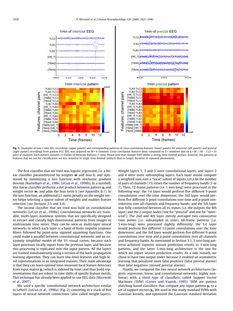
We define in this article a pattern as a structured collection offeatures described in previous section. A pattern groups featuresalong the spatial, time and frequency dimensions. A simplisticanalogy is that a feature is like the color of a pixel at a specific loca-tion in an image. In this article, we formed 2D patterns by aggre-gating features from all 15 pairs of channels (across rows) andover several consecutive time frames (across columns). Specifi-cally, we formed 1 or 5 min-long patterns of 12 or 60 frames,respectively. In the case of frequency-based features, we alsostacked patterns, row-wise and from all frequency ranges intoone pattern. The dimensionality of the feature patterns rangedfrom 180 (e.g. cross-correlation on 1 min windows, Fig. 1), to6300 (e.g. wavelet phase-locking synchrony on 5 min windows).As mentioned in Section 3.1 and 5 min-long patterns achievedsuperior results to 1 min-long patterns, and the article thereforereports seizure prediction results on 5 min-long patterns only.
Throughout the article, we denote as yt a pattern at time t (i.e. asample of bivariate features), and zt the associated label (�1 forpreictal, 1 for interictal). yt can either be one long vector or a ma-trix indexed by time and by channel pair and frequency band.
2.4. Machine learning classification of patterns of bivariate features
Bivariate patterns yt described in previous sections and repre-senting a ‘‘snapshot” of EEG synchronization around time t wereinput into a decision system that would classify them as preictalor interictal. The parameters of that classifier were learned onthe training subset of the dataset using machine learning. Let usnote zt the label of pattern yt (�1 for preictal, 1 for interictal)and �zt the output of the classifier. Although we used three differenttypes of classifiers, with their respective machine learning algo-rithms, all training algorithms had in common minimizing, forevery training sample yt, the error between output �zt and targetzt. The error between the output and the target is one term ofthe loss function: we explain in Section 2.5 the second term (reg-ularization). Finally, and most importantly, test data were set apartduring the training phase: in other words, we validated the perfor-mance of the classifiers on out-of-sample data.
1min of interictal EEG 1min of preictal EEG
1min interictal pattern 1min preictal patternTLB3 TLC2TLB2 TLC2
[HR_7] TLC2[TBB6] TLC2[TBA4] TLC2
TLB2 TLB3[HR_7] TLB3[TBB6] TLB3[TBA4] TLB3[HR_7] TLB2[TBB6] TLB2[TBA4] TLB2
[TBB6] [HR_7][TBA4] [HR_7][TBA4] [TBB6]Fe
atur
es: c
hann
el p
airs
TLB3 TLC2TLB2 TLC2
[HR_7] TLC2[TBB6] TLC2[TBA4] TLC2
TLB2 TLB3[HR_7] TLB3[TBB6] TLB3[TBA4] TLB3[HR_7] TLB2[TBB6] TLB2[TBA4] TLB2
[TBB6] [HR_7][TBA4] [HR_7][TBA4] [TBB6]Fe
atur
es: c
hann
el p
airs
[TBA4]
[TBA6]
[HR_7]
TLB2
TLB3
TLC2
[TBA4]
[TBA6]
[HR_7]
TLB2
TLB3
TLC2
0 2 4 6 8 10 12Time (frames)
0 2 4 6 8 10 12Time (frames)
Fig. 1. Examples of two 1-min EEG recordings (upper panels) and corresponding patterns of cross-correlation features (lower panels) for interictal (left panels) and preictal(right panels) recordings from patient 012. EEG was acquired on M = 6 channels. Cross-correlation features were computed on 5 s windows and on p = M � (M � 1)/2 = 15pairs of channels. Each pattern contains 12 frames of bivariate features (1 min). Please note that channel TLB3 shows a strong, time-limited artifact; however, the patterns offeatures that we use for classification are less sensitive to single time-limited artifacts than to longer duration or repeated phenomena.
1930 P. Mirowski et al. / Clinical Neurophysiology 120 (2009) 1927–1940
The first classifier that we tried was logistic regression, i.e. a lin-ear classifier parameterized by weights w and bias b, and opti-mized by minimizing a loss function with stochastic gradientdescent (Rumelhart et al., 1986; LeCun et al., 1998b). In a nutshell,this linear classifier performs a dot product between pattern yt andweight vector w, and adds the bias term b (see Appendix B.1). Inthe loss function, an additional L1-norm penalty on the weight vec-tor helps selecting a sparse subset of weights and enables featureselection (see Sections 2.5 and 3.4).
The second classifier that we tried was built on convolutionalnetworks (LeCun et al., 1998a). Convolutional networks are train-able, multi-layer, nonlinear systems that are specifically designedto extract and classify high-dimensional patterns from images ormultivariate time series. They can be seen as multi-layer neuralnetworks in which each layer is a bank of finite-impulse responsefilters followed by point-wise sigmoid squashing functions. Onecould make a parallel between convolutional networks and an ex-tremely simplified model of the V1 visual cortex, because eachlayer processes locally inputs from the previous layer, and becausethis processing is replicated over the input pattern. All the layersare trained simultaneously using a version of the back-propagationlearning algorithm. They can learn low-level features and high-le-vel representations in an integrated manner. Their main advantageis that they can learn optimal time-invariant local feature detectorsfrom input matrix yt (which is indexed by time) and thus build rep-resentations that are robust to time shifts of specific feature motifs.This technique has already been applied to raw EEG data (Mirowskiet al., 2007).
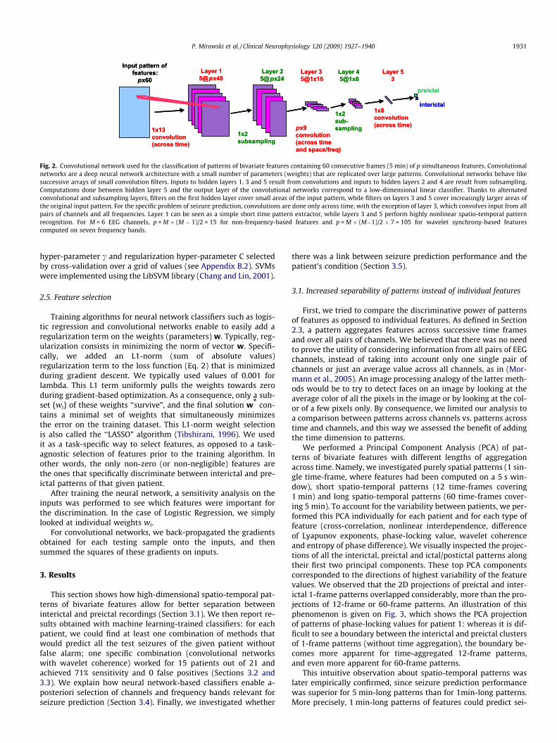
We used a specific convolutional network architecture similarto LeNet5 (LeCun et al., 1998a) (Fig. 2) consisting in a stack of fivelayers of neural network connections (also called weight layers).
Weight layers 1, 3 and 5 were convolutional layers, and layers 2and 4 were mere subsampling layers. Each layer would computea weighted sum over a ‘‘local” subset of inputs. Let p be the numberof pairs of channels (15) times the number of frequency bands (1 or7). Then, 12-frame patterns (i.e. 1 min-long) were processed in thefollowing way: the 1st layer would perform five different 5-pointconvolutions over the time dimension; the 3rd layer would per-form five different 3-point convolutions over time and p-point con-volutions over all channels and frequency bands; and the 5th layerwas fully connected between all its inputs (i.e. the outputs the 4thlayer) and the 2 output nodes (one for ‘‘preictal” and one for ‘‘inter-ictal”). The 2nd and 4th layer merely averaged two consecutivetime points (i.e. subsampled in time). 60-frame patterns (i.e.5 min-long) were processed slightly differently: the 1st layerwould perform five different 13-point convolutions over the timedimension; and the 3rd layer would perform five different 9-pointconvolutions over time and p-point convolutions over all channelsand frequency bands. As mentioned in Section 3.1, 5 min-long pat-terns achieved superior seizure prediction results to 1 min-longpatterns, and the latter 5 min-long architecture is the one forwhich we report seizure prediction results. As a side remark, wechose to have two output nodes because it enabled an asymmetriclearning that penalized more false positives (false preictal alarms)than false negatives (missed preictal alarms).
Finally, we compared the two neural network architectures (lo-gistic regression, linear, and convolutional networks, highly non-linear) with a third type of classifiers, called Support VectorMachines (SVM) (Cortes and Vapnik, 1995). SVM are patternmatching-based classifiers that compare any input pattern yt to aset of support vectors ys. We used in this study standard SVMs withGaussian kernels, and optimized the Gaussian standard deviation
Input pattern of features:px60
Layer 15@px48
Layer 25@px24
Layer 35@1x16
Layer 45@1x8
Layer 53
1x13convolution(across time)
px9convolution(across timeand space/freq)
1x8convolution(across time)
1x2subsampling
1x2sub-sampling
preictal
interictal
Input pattern of features:px60
Layer 15@px48
Layer 25@px24
Layer 35@1x16
Layer 45@1x8
Layer 53
1x13convolution(across time)
px9convolution(across timeand space/freq)
1x8convolution(across time)
1x2subsampling
1x2sub-sampling
preictal
interictal
Fig. 2. Convolutional network used for the classification of patterns of bivariate features containing 60 consecutive frames (5 min) of p simultaneous features. Convolutionalnetworks are a deep neural network architecture with a small number of parameters (weights) that are replicated over large patterns. Convolutional networks behave likesuccessive arrays of small convolution filters. Inputs to hidden layers 1, 3 and 5 result from convolutions and inputs to hidden layers 2 and 4 are result from subsampling.Computations done between hidden layer 5 and the output layer of the convolutional networks correspond to a low-dimensional linear classifier. Thanks to alternatedconvolutional and subsampling layers, filters on the first hidden layer cover small areas of the input pattern, while filters on layers 3 and 5 cover increasingly larger areas ofthe original input pattern. For the specific problem of seizure prediction, convolutions are done only across time, with the exception of layer 3, which convolves input from allpairs of channels and all frequencies. Layer 1 can be seen as a simple short time pattern extractor, while layers 3 and 5 perform highly nonlinear spatio-temporal patternrecognition. For M = 6 EEG channels, p = M � (M � 1)/2 = 15 for non-frequency-based features and p = M � (M�1)/2 � 7 = 105 for wavelet synchrony-based featurescomputed on seven frequency bands.
P. Mirowski et al. / Clinical Neurophysiology 120 (2009) 1927–1940 1931
hyper-parameter c and regularization hyper-parameter C selectedby cross-validation over a grid of values (see Appendix B.2). SVMswere implemented using the LibSVM library (Chang and Lin, 2001).
2.5. Feature selection
Training algorithms for neural network classifiers such as logis-tic regression and convolutional networks enable to easily add aregularization term on the weights (parameters) w. Typically, reg-ularization consists in minimizing the norm of vector w. Specifi-cally, we added an L1-norm (sum of absolute values)regularization term to the loss function (Eq. 2) that is minimizedduring gradient descent. We typically used values of 0.001 forlambda. This L1 term uniformly pulls the weights towards zeroduring gradient-based optimization. As a consequence, only a sub-set {wi} of these weights ‘‘survive”, and the final solution w* con-tains a minimal set of weights that simultaneously minimizesthe error on the training dataset. This L1-norm weight selectionis also called the ‘‘LASSO” algorithm (Tibshirani, 1996). We usedit as a task-specific way to select features, as opposed to a task-agnostic selection of features prior to the training algorithm. Inother words, the only non-zero (or non-negligible) features arethe ones that specifically discriminate between interictal and pre-ictal patterns of that given patient.
After training the neural network, a sensitivity analysis on theinputs was performed to see which features were important forthe discrimination. In the case of Logistic Regression, we simplylooked at individual weights wi.
For convolutional networks, we back-propagated the gradientsobtained for each testing sample onto the inputs, and thensummed the squares of these gradients on inputs.
3. Results
This section shows how high-dimensional spatio-temporal pat-terns of bivariate features allow for better separation betweeninterictal and preictal recordings (Section 3.1). We then report re-sults obtained with machine learning-trained classifiers: for eachpatient, we could find at least one combination of methods thatwould predict all the test seizures of the given patient withoutfalse alarm; one specific combination (convolutional networkswith wavelet coherence) worked for 15 patients out of 21 andachieved 71% sensitivity and 0 false positives (Sections 3.2 and3.3). We explain how neural network-based classifiers enable a-posteriori selection of channels and frequency bands relevant forseizure prediction (Section 3.4). Finally, we investigated whether
there was a link between seizure prediction performance and thepatient’s condition (Section 3.5).
3.1. Increased separability of patterns instead of individual features
First, we tried to compare the discriminative power of patternsof features as opposed to individual features. As defined in Section2.3, a pattern aggregates features across successive time framesand over all pairs of channels. We believed that there was no needto prove the utility of considering information from all pairs of EEGchannels, instead of taking into account only one single pair ofchannels or just an average value across all channels, as in (Mor-mann et al., 2005). An image processing analogy of the latter meth-ods would be to try to detect faces on an image by looking at theaverage color of all the pixels in the image or by looking at the col-or of a few pixels only. By consequence, we limited our analysis toa comparison between patterns across channels vs. patterns acrosstime and channels, and this way we assessed the benefit of addingthe time dimension to patterns.
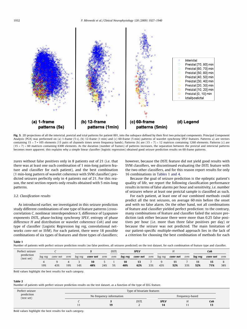
We performed a Principal Component Analysis (PCA) of pat-terns of bivariate features with different lengths of aggregationacross time. Namely, we investigated purely spatial patterns (1 sin-gle time-frame, where features had been computed on a 5 s win-dow), short spatio-temporal patterns (12 time-frames covering1 min) and long spatio-temporal patterns (60 time-frames cover-ing 5 min). To account for the variability between patients, we per-formed this PCA individually for each patient and for each type offeature (cross-correlation, nonlinear interdependence, differenceof Lyapunov exponents, phase-locking value, wavelet coherenceand entropy of phase difference). We visually inspected the projec-tions of all the interictal, preictal and ictal/postictal patterns alongtheir first two principal components. These top PCA componentscorresponded to the directions of highest variability of the featurevalues. We observed that the 2D projections of preictal and inter-ictal 1-frame patterns overlapped considerably, more than the pro-jections of 12-frame or 60-frame patterns. An illustration of thisphenomenon is given on Fig. 3, which shows the PCA projectionof patterns of phase-locking values for patient 1: whereas it is dif-ficult to see a boundary between the interictal and preictal clustersof 1-frame patterns (without time aggregation), the boundary be-comes more apparent for time-aggregated 12-frame patterns,and even more apparent for 60-frame patterns.
This intuitive observation about spatio-temporal patterns waslater empirically confirmed, since seizure prediction performancewas superior for 5 min-long patterns than for 1min-long patterns.More precisely, 1 min-long patterns of features could predict sei-
a) 1-framepatterns (5s)
b) 12-framepatterns (1min)
c) 60-framepatterns (5min)
d) Legenda) 1-framepatterns (5s)
b) 12-framepatterns (1min)
c) 60-framepatterns (5min)
d) Legend) ) ) )
Fig. 3. 2D projections of all the interictal, preictal and ictal patterns for patient 001, into the subspace defined by their first two principal components. Principal ComponentAnalysis (PCA) was performed on (a) 1-frame (5 s), (b) 12-frame (1 min) and (c) 60-frame (5 min) patterns of wavelet synchrony SPLV features. Patterns a) are vectorscontaining 15 � 7 = 105 elements (15 pairs of channels times seven frequency bands). Patterns (b) are (15 � 7) � 12 matrices containing 1260 elements. Patterns (c) are(15 � 7) � 60 matrices containing 6300 elements. As the duration (number of frames) of patterns increases, the separation between the preictal and interictal patternsbecomes more apparent; this explains why a simple linear classifier (logistic regression) obtained good seizure prediction results on 60-frame patterns.
1932 P. Mirowski et al. / Clinical Neurophysiology 120 (2009) 1927–1940
zures without false positives only in 8 patients out of 21 (i.e. thatthere was at least one such combination of 1 min-long pattern fea-ture and classifier for each patient), and the best combination(1 min-long pattern of wavelet coherence with SVM classifier) pre-dicted seizures perfectly only in 4 patients out of 21. For this rea-son, the next section reports only results obtained with 5 min-longpatterns.
3.2. Classification results
As introduced earlier, we investigated in this seizure predictionstudy different combinations of one type of feature patterns (cross-correlation C, nonlinear interdependence S, difference of Lyapunovexponents DSTL, phase-locking synchrony SPLV, entropy of phasedifference H and distribution or wavelet coherence Coh) and onetype of classifier (Logistic Regression log reg, convolutional net-works conv-net or SVM). For each patient, there were 18 possiblecombinations of six types of features and three types of classifiers;
Table 1Number of patients with perfect seizure prediction results (no false positives, all seizures
Perfect seizureprediction(test set)
C S DSTL
log reg conv net svm log reg conv net svm svm log
4 9 4 3 10 5 1 119% 43% 19% 14% 48% 24% 5% 4
Bold values highlight the best results for each category.
Table 2Number of patients with perfect seizure prediction results on the test dataset, as a functi
Perfect seizureprediction(test set)
No frequency information
C S11 19
Bold values highlight the best results for each category.
however, because the DSTL feature did not yield good results withSVM classifiers, we discontinued evaluating the DSTL feature withthe two other classifiers, and for this reason report results for only16 combinations in Tables 1 and 4.
Because the goal of seizure prediction is the epileptic patient’squality of life, we report the following classification performanceresults in terms of false alarms per hour and sensitivity, i.e. numberof seizures where at least one preictal sample is classified as such.
For each patient, at least one of our combined methods couldpredict all the test seizures, on average 60 min before the onsetand with no false alarm. On the other hand, not all combinationsof feature and classifier yielded perfect prediction: to the contrary,many combinations of feature and classifier failed the seizure pre-diction task either because there were more than 0.25 false posi-tives per hour (i.e. more than three false positives per day) orbecause the seizure was not predicted. The main limitation ofour patient-specific multiple-method approach lies in the lack ofa criterion for choosing the best combination of methods for each
predicted) on the test dataset, for each combination of feature type and classifier.
SPLV H Coh
reg conv net svm log reg conv net svm log reg conv net svm
0 13 7 9 11 7 11 15 88% 62% 33% 43% 52% 33% 52% 71% 38%
on of the type of EEG feature.
Type of bivariate features
Frequency-based
DSTL SPLV H Coh2 14 11 13
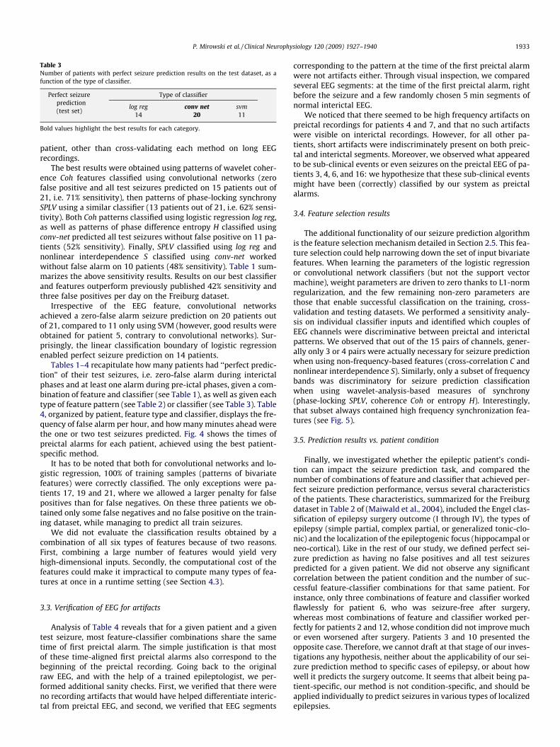
Table 3Number of patients with perfect seizure prediction results on the test dataset, as afunction of the type of classifier.
Perfect seizureprediction(test set)
Type of classifier
log reg conv net svm14 20 11
Bold values highlight the best results for each category.
P. Mirowski et al. / Clinical Neurophysiology 120 (2009) 1927–1940 1933
patient, other than cross-validating each method on long EEGrecordings.
The best results were obtained using patterns of wavelet coher-ence Coh features classified using convolutional networks (zerofalse positive and all test seizures predicted on 15 patients out of21, i.e. 71% sensitivity), then patterns of phase-locking synchronySPLV using a similar classifier (13 patients out of 21, i.e. 62% sensi-tivity). Both Coh patterns classified using logistic regression log reg,as well as patterns of phase difference entropy H classified usingconv-net predicted all test seizures without false positive on 11 pa-tients (52% sensitivity). Finally, SPLV classified using log reg andnonlinear interdependence S classified using conv-net workedwithout false alarm on 10 patients (48% sensitivity). Table 1 sum-marizes the above sensitivity results. Results on our best classifierand features outperform previously published 42% sensitivity andthree false positives per day on the Freiburg dataset.
Irrespective of the EEG feature, convolutional networksachieved a zero-false alarm seizure prediction on 20 patients outof 21, compared to 11 only using SVM (however, good results wereobtained for patient 5, contrary to convolutional networks). Sur-prisingly, the linear classification boundary of logistic regressionenabled perfect seizure prediction on 14 patients.
Tables 1–4 recapitulate how many patients had ‘‘perfect predic-tion” of their test seizures, i.e. zero-false alarm during interictalphases and at least one alarm during pre-ictal phases, given a com-bination of feature and classifier (see Table 1), as well as given eachtype of feature pattern (see Table 2) or classifier (see Table 3). Table4, organized by patient, feature type and classifier, displays the fre-quency of false alarm per hour, and how many minutes ahead werethe one or two test seizures predicted. Fig. 4 shows the times ofpreictal alarms for each patient, achieved using the best patient-specific method.
It has to be noted that both for convolutional networks and lo-gistic regression, 100% of training samples (patterns of bivariatefeatures) were correctly classified. The only exceptions were pa-tients 17, 19 and 21, where we allowed a larger penalty for falsepositives than for false negatives. On these three patients we ob-tained only some false negatives and no false positive on the train-ing dataset, while managing to predict all train seizures.
We did not evaluate the classification results obtained by acombination of all six types of features because of two reasons.First, combining a large number of features would yield veryhigh-dimensional inputs. Secondly, the computational cost of thefeatures could make it impractical to compute many types of fea-tures at once in a runtime setting (see Section 4.3).
3.3. Verification of EEG for artifacts
Analysis of Table 4 reveals that for a given patient and a giventest seizure, most feature-classifier combinations share the sametime of first preictal alarm. The simple justification is that mostof these time-aligned first preictal alarms also correspond to thebeginning of the preictal recording. Going back to the originalraw EEG, and with the help of a trained epileptologist, we per-formed additional sanity checks. First, we verified that there wereno recording artifacts that would have helped differentiate interic-tal from preictal EEG, and second, we verified that EEG segments
corresponding to the pattern at the time of the first preictal alarmwere not artifacts either. Through visual inspection, we comparedseveral EEG segments: at the time of the first preictal alarm, rightbefore the seizure and a few randomly chosen 5 min segments ofnormal interictal EEG.
We noticed that there seemed to be high frequency artifacts onpreictal recordings for patients 4 and 7, and that no such artifactswere visible on interictal recordings. However, for all other pa-tients, short artifacts were indiscriminately present on both preic-tal and interictal segments. Moreover, we observed what appearedto be sub-clinical events or even seizures on the preictal EEG of pa-tients 3, 4, 6, and 16: we hypothesize that these sub-clinical eventsmight have been (correctly) classified by our system as preictalalarms.
3.4. Feature selection results
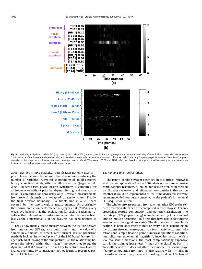
The additional functionality of our seizure prediction algorithmis the feature selection mechanism detailed in Section 2.5. This fea-ture selection could help narrowing down the set of input bivariatefeatures. When learning the parameters of the logistic regressionor convolutional network classifiers (but not the support vectormachine), weight parameters are driven to zero thanks to L1-normregularization, and the few remaining non-zero parameters arethose that enable successful classification on the training, cross-validation and testing datasets. We performed a sensitivity analy-sis on individual classifier inputs and identified which couples ofEEG channels were discriminative between preictal and interictalpatterns. We observed that out of the 15 pairs of channels, gener-ally only 3 or 4 pairs were actually necessary for seizure predictionwhen using non-frequency-based features (cross-correlation C andnonlinear interdependence S). Similarly, only a subset of frequencybands was discriminatory for seizure prediction classificationwhen using wavelet-analysis-based measures of synchrony(phase-locking SPLV, coherence Coh or entropy H). Interestingly,that subset always contained high frequency synchronization fea-tures (see Fig. 5).
3.5. Prediction results vs. patient condition
Finally, we investigated whether the epileptic patient’s condi-tion can impact the seizure prediction task, and compared thenumber of combinations of feature and classifier that achieved per-fect seizure prediction performance, versus several characteristicsof the patients. These characteristics, summarized for the Freiburgdataset in Table 2 of (Maiwald et al., 2004), included the Engel clas-sification of epilepsy surgery outcome (I through IV), the types ofepilepsy (simple partial, complex partial, or generalized tonic-clo-nic) and the localization of the epileptogenic focus (hippocampal orneo-cortical). Like in the rest of our study, we defined perfect sei-zure prediction as having no false positives and all test seizurespredicted for a given patient. We did not observe any significantcorrelation between the patient condition and the number of suc-cessful feature-classifier combinations for that same patient. Forinstance, only three combinations of feature and classifier workedflawlessly for patient 6, who was seizure-free after surgery,whereas most combinations of feature and classifier worked per-fectly for patients 2 and 12, whose condition did not improve muchor even worsened after surgery. Patients 3 and 10 presented theopposite case. Therefore, we cannot draft at that stage of our inves-tigations any hypothesis, neither about the applicability of our sei-zure prediction method to specific cases of epilepsy, or about howwell it predicts the surgery outcome. It seems that albeit being pa-tient-specific, our method is not condition-specific, and should beapplied individually to predict seizures in various types of localizedepilepsies.
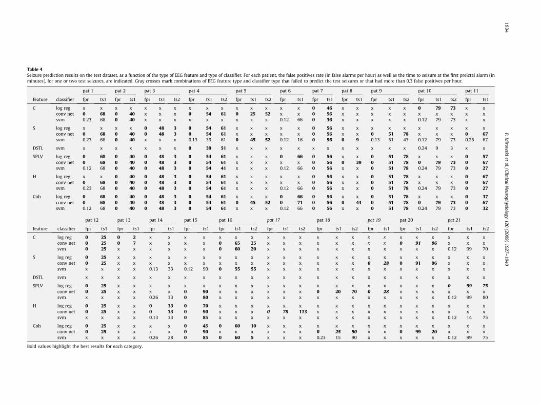
Table 4Seizure prediction results on the test dataset, as a function of the type of EEG feature and type of classifier. For each patient, the false positives rate (in false alarms per hour) as well as the time to seizure at the first preictal alarm (inminutes), for one or two test seizures, are indicated. Gray crosses mark combinations of EEG feature type and classifier type that failed to predict the test seizures or that had more than 0.3 false positives per hour.
pat 1 pat 2 pat 3 pat 4 pat 5 pat 6 pat 7 pat 8 pat 9 pat 10 pat 11
feature classifier fpr ts1 fpr ts1 fpr ts1 ts2 fpr ts1 ts2 fpr ts1 ts2 fpr ts1 fpr ts1 fpr ts1 fpr ts1 ts2 fpr ts1 ts2 fpr ts1
C log reg x x x x x x x x x x x x x x x 0 46 x x x x x 0 79 73 x xconv net 0 68 0 40 x x x 0 54 61 0 25 52 x x 0 56 x x x x x x x x x xsvm 0.23 68 0 40 x x x x x x x x x 0.12 66 0 36 x x x x x 0.12 79 73 x x
S log reg x x x x 0 48 3 0 54 61 x x x x x 0 56 x x x x x x x x x xconv net 0 68 0 40 0 48 3 0 54 61 x x x x x 0 56 x x 0 51 78 x x x 0 67svm 0.23 68 0 40 x x x 0.13 39 61 0 45 52 0.12 16 0 56 0 9 0.13 51 43 0.12 79 73 0.25 67
DSTL svm x x x x x x x 0 39 51 x x x x x x x x x x x x 0.24 9 3 x x
SPLV log reg 0 68 0 40 0 48 3 0 54 61 x x x 0 66 0 56 x x 0 51 78 x x x 0 57conv net 0 68 0 40 0 48 3 0 54 61 x x x x x 0 56 0 39 0 51 78 0 79 73 0 67svm 0.12 68 0 40 0 48 3 0 54 41 x x x 0.12 66 0 56 x x 0 51 78 0.24 79 73 0 27
H log reg x x 0 40 0 48 3 0 54 61 x x x x x 0 56 x x 0 51 78 x x x 0 67conv net 0 68 0 40 0 48 3 0 54 61 x x x x x 0 56 x x 0 51 78 x x x 0 67svm 0.23 68 0 40 0 48 3 0 54 61 x x x 0.12 66 0 56 x x 0 51 78 0.24 79 73 0 27
Coh log reg 0 68 0 40 0 48 3 0 54 61 x x x 0 66 0 56 x x 0 51 78 x x x 0 37conv net 0 68 0 40 0 48 3 0 54 61 0 45 52 0 71 0 56 0 44 0 51 78 0 79 73 0 67svm 0.12 68 0 40 0 48 3 0 54 61 x x x 0.12 66 0 56 x x 0 51 78 0.24 79 73 0 32
pat 12 pat 13 pat 14 pat 15 pat 16 pat 17 pat 18 pat 19 pat 20 pat 21
feature classifier fpr ts1 fpr ts1 fpr ts1 fpr ts1 fpr ts1 ts2 fpr ts1 ts2 fpr ts1 ts2 fpr ts1 fpr ts1 ts2 fpr ts1 ts2
C log reg 0 25 0 2 x x x x x x x x x x x x x x x x x x x x xconv net 0 25 0 7 x x x x 0 65 25 x x x x x x x x 0 91 96 x x xsvm 0 25 x x x x x x 0 60 20 x x x x x x x x x x x 0.12 99 70
S log reg 0 25 x x x x x x x x x x x x x x x x x x x x x x xconv net 0 25 x x x x x x x x x x x x x x x 0 28 0 91 96 x x xsvm x x x x 0.13 33 0.12 90 0 55 55 x x x x x x x x x x x x x x
DSTL svm x x x x x x x x x x x x x x x x x x x x x x x x x
SPLV log reg 0 25 x x x x x x x x x x x x x x x x x x x x 0 99 75conv net 0 25 x x x x 0 90 x x x x x x 0 20 70 0 28 x x x x x xsvm x x x x 0.26 33 0 80 x x x x x x x x x x x x x x 0.12 99 80
H log reg 0 25 x x 0 33 0 70 x x x x x x x x x x x x x x x x xconv net 0 25 x x 0 33 0 90 x x x 0 78 113 x x x x x x x x x x xsvm x x x x 0.13 33 0 85 x x x x x x x x x x x x x x 0.12 14 75
Coh log reg 0 25 x x x x 0 45 0 60 10 x x x x x x x x x x x x x xconv net 0 25 x x x x 0 90 x x x x x x 0 25 90 x x 0 99 20 x x xsvm x x x x 0.26 28 0 85 0 60 5 x x x 0.23 15 90 x x x x x 0.12 99 75
Bold values highlight the best results for each category.
1934P.M
irowski
etal./Clinical
Neurophysiology
120(2009)
1927–1940
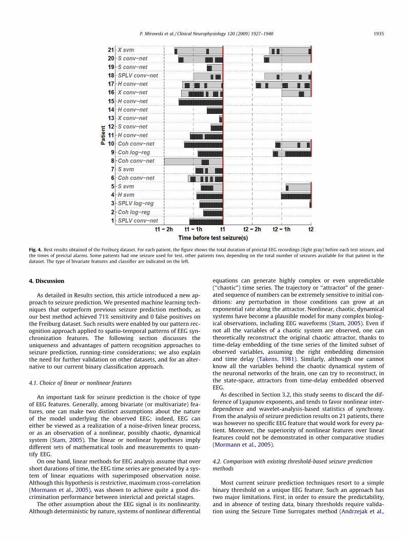
Fig. 4. Best results obtained of the Freiburg dataset. For each patient, the figure shows the total duration of preictal EEG recordings (light gray) before each test seizure, andthe times of preictal alarms. Some patients had one seizure used for test, other patients two, depending on the total number of seizures available for that patient in thedataset. The type of bivariate features and classifier are indicated on the left.
P. Mirowski et al. / Clinical Neurophysiology 120 (2009) 1927–1940 1935
4. Discussion
As detailed in Results section, this article introduced a new ap-proach to seizure prediction. We presented machine learning tech-niques that outperform previous seizure prediction methods, asour best method achieved 71% sensitivity and 0 false positives onthe Freiburg dataset. Such results were enabled by our pattern rec-ognition approach applied to spatio-temporal patterns of EEG syn-chronization features. The following section discusses theuniqueness and advantages of pattern recognition approaches toseizure prediction, running-time considerations; we also explainthe need for further validation on other datasets, and for an alter-native to our current binary classification approach.
4.1. Choice of linear or nonlinear features
An important task for seizure prediction is the choice of typeof EEG features. Generally, among bivariate (or multivariate) fea-tures, one can make two distinct assumptions about the natureof the model underlying the observed EEG; indeed, EEG caneither be viewed as a realization of a noise-driven linear process,or as an observation of a nonlinear, possibly chaotic, dynamicalsystem (Stam, 2005). The linear or nonlinear hypotheses implydifferent sets of mathematical tools and measurements to quan-tify EEG.
On one hand, linear methods for EEG analysis assume that overshort durations of time, the EEG time series are generated by a sys-tem of linear equations with superimposed observation noise.Although this hypothesis is restrictive, maximum cross-correlation(Mormann et al., 2005), was shown to achieve quite a good dis-crimination performance between interictal and preictal stages.
The other assumption about the EEG signal is its nonlinearity.Although deterministic by nature, systems of nonlinear differential
equations can generate highly complex or even unpredictable(‘‘chaotic”) time series. The trajectory or ‘‘attractor” of the gener-ated sequence of numbers can be extremely sensitive to initial con-ditions: any perturbation in those conditions can grow at anexponential rate along the attractor. Nonlinear, chaotic, dynamicalsystems have become a plausible model for many complex biolog-ical observations, including EEG waveforms (Stam, 2005). Even ifnot all the variables of a chaotic system are observed, one cantheoretically reconstruct the original chaotic attractor, thanks totime-delay embedding of the time series of the limited subset ofobserved variables, assuming the right embedding dimensionand time delay (Takens, 1981). Similarly, although one cannotknow all the variables behind the chaotic dynamical system ofthe neuronal networks of the brain, one can try to reconstruct, inthe state-space, attractors from time-delay embedded observedEEG.
As described in Section 3.2, this study seems to discard the dif-ference of Lyapunov exponents, and tends to favor nonlinear inter-dependence and wavelet-analysis-based statistics of synchrony.From the analysis of seizure prediction results on 21 patients, therewas however no specific EEG feature that would work for every pa-tient. Moreover, the superiority of nonlinear features over linearfeatures could not be demonstrated in other comparative studies(Mormann et al., 2005).
4.2. Comparison with existing threshold-based seizure predictionmethods
Most current seizure prediction techniques resort to a simplebinary threshold on a unique EEG feature. Such an approach hastwo major limitations. First, in order to ensure the predictability,and in absence of testing data, binary thresholds require valida-tion using the Seizure Time Surrogates method (Andrzejak et al.,
Time (frames)
intrafocal
focal-extrafocal
extrafocal
focal-extrafocal
extrafocal
0 10 20 30 40 50 60
5
10
15
0
TLB3 TLC2TLB2 TLC2
[HR_7] TLC2[TBB6] TLC2[TBA4] TLC2
TLB2 TLB3[HR_7] TLB3[TBB6] TLB3[TBA4] TLB3[HR_7] TLB2[TBB6] TLB2[TBA4] TLB2
[TBB6] [HR_7][TBA4] [HR_7][TBA4] [TBB6]
(a)
δ (< 4Hz)
0 10 20 30 40 50 60
2
3
4
1
0
θ (4Hz – 7Hz)
α(7Hz – 13Hz)
Low β (13Hz – 15Hz)
High β (14Hz – 30Hz)
Low γ (31-45Hz)
High γ (55-100Hz)
Time (frames)(b)
Fig. 5. Sensitivity analysis for patient 012 (top panel a) and patient 008 (bottom panel b). Both images represent the input sensitivity of convolutional networks performed on5 min patterns of nonlinear interdependence (a) and wavelet coherence (b), respectively. Wavelet coherence in (b) is the only frequency-specific feature. Classifier (a) appearssensitive to interdependence features measure between two extrafocal EEG channels TLB2 and TLB3, whereas classifier (b) appears sensitive mostly to synchronizationfeatures in the high gamma range and in the alpha range.
1936 P. Mirowski et al. / Clinical Neurophysiology 120 (2009) 1927–1940
2003). Besides, simple statistical classification not only uses sim-plistic linear decision boundaries, but also requires reducing thenumber of variables. A typical shortcoming of an ill-designedbinary classification algorithm is illustrated in (Jerger et al.,2005). Hilbert-based phase-locking synchrony is computed forall frequencies without prior band-pass filtering, and cross-corre-lation is computed for zero delay only. Bivariate measurementsfrom several channels are collapsed to single values. Finally,the final decision boundary is a simple line in a 2D spacecovered by the two bivariate measurements. Unsurprisingly,the seizure prediction performance of (Jerger et al., 2005) is veryweak. We believe that the explanation for such unsatisfying re-sults is that relevant seizure-discriminative information has beenlost as the dimensionality of the features has been reduced totwo.
Let us now make a crude analogy between the feature derivedfrom one or two EEG signals around time t, and the value of a‘‘pixel” in a ‘‘movie” at time t. Most current seizure predictionmethods look at ‘‘individual pixels” of the EEG-based feature ‘‘im-age” instead of looking at the ‘‘full picture”, i.e. the relationship be-tween the ‘‘pixels” within that ‘‘image”; moreover they forego thedynamics of that ‘‘movie”, i.e. do not try to capture how featureschange over time. By contrast, our method learns to recognize pat-terns of EEG features.
4.3. Running-time considerations
The patent-pending system described in this article (Mirowskiet al., patent application filed in 2009) does not require extensivecomputational resources. Although our seizure prediction methodis still under evaluation and refinement, we consider in this sectionwhether it could be implemented as real-time dedicated softwareon an embedded computer connected to the patient’s intracranialEEG acquisition system.
The whole software process, from raw numerical EEG to the sei-zure prediction alarm can be decomposed in three stages: EEG pre-processing, feature computation and pattern classification. Thefirst stage (EEG preprocessing) is implemented by four standardInfinite Impulse Response (IIR) filters that have negligible runtimeeven in real-time signal processing. The third stage (pattern classi-fication) is done only every minute or every 5 min (depending onthe pattern size) and corresponds to a few matrix-vector multipli-cations and simple floating-point numerical operations (addition,multiplication, exponential, logarithm), involving vectors with afew thousand dimensions. The most computationally expensivepart is the training (parameter fitting) of the classifier, but it isdone offline and thus does not affect the runtime. The second stage(feature computation from EEG) is also relatively fast: it takes inthe order of seconds to process a 5 min-long window of 6-channel
P. Mirowski et al. / Clinical Neurophysiology 120 (2009) 1927–1940 1937
EEG and extract features such as wavelet-analysis-based syn-chrony (SPLV, Coh or H), nonlinear interdependence S or cross-cor-relation C. However, since the 5 min patterns are not overlapping,stage 2 is only repeated every minute or 5 min (like stage 3). It hasto be noted that this running-time analysis was done on a softwareprototype that could be further optimized for speed.
The software for computing features from EEG was imple-mented in MatlabTM and can be run under its free open-sourcecounterpart, OctaveTM. Support vector machine classification wasperformed using LibSVMTM (Chang and Lin, 2001) and its Matlab/Octave interface. Convolutional networks and logistic regressionwere implemented in LushTM, an open-source programming envi-ronment (Bottou and LeCun, 2002) with extensive machine learn-ing libraries.
4.4. Overcoming high number of EEG channels through featureselection
In addition to real-time capabilities during runtime, the trainingphase of the classifier has an additional benefit. Our seizure predic-tion method enables further feature selection through sensitivityanalysis, namely the discovery of subsets of channels (and if rele-vant, frequencies of analysis), that have a strong discriminativepower for the preictal versus interictal classification task.
This capability could help the system cope with a high numberof EEG channels. Indeed, the number of bivariate features growsquadratically with the number of channels M, and this quadraticdependence on the number of EEG channels becomes problematicwhen EEG recordings contain many channels, e.g. one or two 64-channel grids with additional strip electrodes. This limitationmight slow down both the machine learning (training) and eventhe runtime (testing) phases. Through sensitivity analysis, onecould narrow down the subset of EEG channels necessary for agood seizure prediction performance. One could envision the fol-lowing approach: first, long and slow training and evaluationphases using all the EEG channels, followed by channel selectionwith respect to their discriminative power, and a second, faster,training phase, with, as end product, a seizure prediction classifierrunning on a restricted number of EEG channels. The main advan-tage of this approach is that the channel selection is done a-poste-riori with respect to the seizure prediction performance, and not apriori as in previous studies (D’Alessandro et al., 2003; Le Van Quy-en et al., 2005). In our method, the classifier decides by itself whichsubset of channels is the most appropriate.
4.5. Statistical validity
One of the recommended validation methods for seizure predic-tion algorithms is Seizure Time Surrogates (STS) (Andrzejak et al.,2003). As stated in the introduction, STS is a necessary validationstep required by most current statistical seizure prediction meth-ods, which use all available data to find the boundary thresholds(in-sample optimization using the ROC curve) without properout-of-sample testing. STS consists in repeatedly scrambling thepreictal and interictal labels and checking that the subsequent fakedecision boundaries are statistically different from the true deci-sion boundary.
Such surrogate methods are however virtually unknown in theabundant machine learning literature and its countless applica-tions, because the validation of machine learning algorithms reliesinstead on the Statistical Learning Theory (Vapnik, 1995). The lat-ter consists in regularizing the parameters of the classifier (as de-scribed in Section 2.5), and in separating the dataset into atraining and cross-validation set for parameter optimization, anda testing set that is unseen during the optimization phase (as de-scribed in details in Section 2.1).
On one hand, the use of a carefully designed separate and un-seen testing set verifies that the classifier works well in the generalcase, within the limits of the testing dataset. Given the long timerequired to train a machine learning classifier, such an approachis less computationally expensive than surrogate methods.
On the other hand, the regularization permits to choose, amongthe infinity of configurations of parameter values (e.g. the ‘‘synap-tic” connection weights of a convolutional network or the matrix oflogistic regression), the ‘‘simplest” one, generally satisfying a crite-rion such as choosing the feasible parameter vector with the small-est norm. The regularized classifier does not overfit the trainingdataset (e.g. it does not learn the training set patterns ‘‘by heart”)but has instead good generalization properties, i.e. a low theoreti-cal error on unseen testing set patterns. Moreover, regularizationenables to cope with datasets where the number of inputs is great-er than the number of training instances. This is for instance thecase with machine learning-based classification of biological data,where very few micro-array measurements (each micro-arraybeing a single instance in the learning dataset) contain tens ofthousands of genes or protein expression levels.
Nevertheless, let us devise the following combinatorial verifica-tion of the results. Since our study focused on non-overlapping5 min-long patterns, and since our patient-specific predictorswould ignore the time stamp of each pattern, we consider a ran-dom predictor that gives independent predictions every 5 min onone patient’s data, and emits a preictal alarm with probability p.Each patient’s recording consists of at least 24 h of interictal data(out of which, at least 8 h are set apart for testing), which contain,respectively, at least ni = 288 or ni = 96 patterns, and m preictalrecordings of at most 2 h each (out of which, one or two are setapart for testing), with at most np = 24 patterns per preictal record-ing. Using binomial distributions, we can compute the probability:AðpÞ ¼ f ð0; ni; pÞ of not emitting any alarm during the interictalphase, as well as the probability of emitting at least one alarm be-fore each seizure: BðpÞ ¼ 1� f ð0; np; pÞ. The probability of predict-ing each seizure of a patient, without false alarm, is a function ofthe predictor’s p: CðpÞ ¼ AðpÞBðpÞm.
After maximization with respect to the random predictor ‘‘firingrate” p, the optimal random predictor could predict, without falsealarm during the 8 h of out-of-sample interictal recording, one testseizure with over 8% probability and two test seizures with over2% probability. In our study, we evaluated 16 different combinationsof features and classifiers. If one tried 16 different random predictorsfor a given patient, and using again binomial distributions, the ex-pected number of successful predictions would be computed as1.3 for one test seizure, and 0.4 for two test seizures. Consideringthat the random predictor also needs to correctly classify patternsfrom the training and cross-validation dataset, in other words tocorrectly predict the entire patient’s dataset (this was the case ofthe successful classifiers reported in Table 1), then, by a similar argu-ment, this expected number of successful predictions goes downfrom 0.05 for a 2-seizures dataset to 10�4 for a 6-seizures dataset.
Although the above combinatorial analysis only gives an upperbound on the number of ‘‘successful” random predictors for a givenpatient, it motivates a critical look at the results reported in Table4. Specifically, seizure prediction results obtained for certain pa-tients where only 1 or 2 classifiers (out of 16) succeeded in predict-ing without false alarm should be considered with reserve (such isthe case for patients 13, 17, 19 and 21).
4.6. Limitations of binary classification for seizure prediction
A second limitation of our method lies in our binary classifica-tion approach. When attempting seizure prediction, binary classi-fication is both a simplification and an additional challenge fortraining the classifier. In our case, 2-h-long preictal periods imply
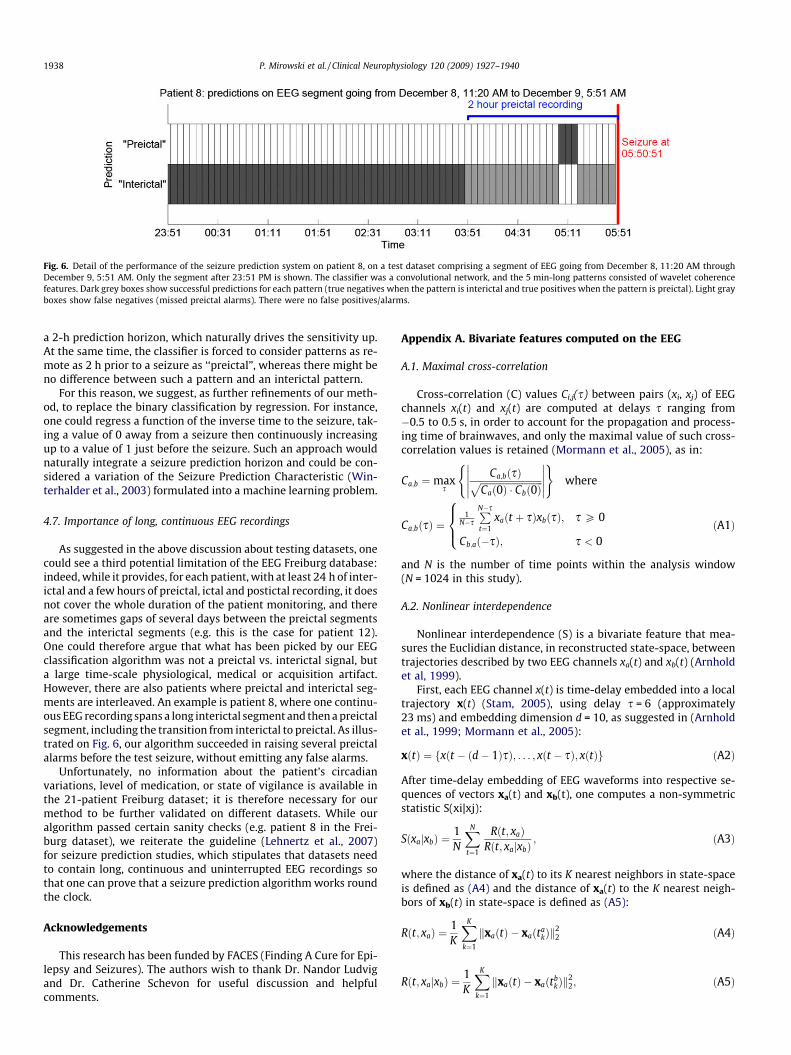
Fig. 6. Detail of the performance of the seizure prediction system on patient 8, on a test dataset comprising a segment of EEG going from December 8, 11:20 AM throughDecember 9, 5:51 AM. Only the segment after 23:51 PM is shown. The classifier was a convolutional network, and the 5 min-long patterns consisted of wavelet coherencefeatures. Dark grey boxes show successful predictions for each pattern (true negatives when the pattern is interictal and true positives when the pattern is preictal). Light grayboxes show false negatives (missed preictal alarms). There were no false positives/alarms.
1938 P. Mirowski et al. / Clinical Neurophysiology 120 (2009) 1927–1940
a 2-h prediction horizon, which naturally drives the sensitivity up.At the same time, the classifier is forced to consider patterns as re-mote as 2 h prior to a seizure as ‘‘preictal”, whereas there might beno difference between such a pattern and an interictal pattern.
For this reason, we suggest, as further refinements of our meth-od, to replace the binary classification by regression. For instance,one could regress a function of the inverse time to the seizure, tak-ing a value of 0 away from a seizure then continuously increasingup to a value of 1 just before the seizure. Such an approach wouldnaturally integrate a seizure prediction horizon and could be con-sidered a variation of the Seizure Prediction Characteristic (Win-terhalder et al., 2003) formulated into a machine learning problem.
4.7. Importance of long, continuous EEG recordings
As suggested in the above discussion about testing datasets, onecould see a third potential limitation of the EEG Freiburg database:indeed, while it provides, for each patient, with at least 24 h of inter-ictal and a few hours of preictal, ictal and postictal recording, it doesnot cover the whole duration of the patient monitoring, and thereare sometimes gaps of several days between the preictal segmentsand the interictal segments (e.g. this is the case for patient 12).One could therefore argue that what has been picked by our EEGclassification algorithm was not a preictal vs. interictal signal, buta large time-scale physiological, medical or acquisition artifact.However, there are also patients where preictal and interictal seg-ments are interleaved. An example is patient 8, where one continu-ous EEG recording spans a long interictal segment and then a preictalsegment, including the transition from interictal to preictal. As illus-trated on Fig. 6, our algorithm succeeded in raising several preictalalarms before the test seizure, without emitting any false alarms.
Unfortunately, no information about the patient’s circadianvariations, level of medication, or state of vigilance is available inthe 21-patient Freiburg dataset; it is therefore necessary for ourmethod to be further validated on different datasets. While ouralgorithm passed certain sanity checks (e.g. patient 8 in the Frei-burg dataset), we reiterate the guideline (Lehnertz et al., 2007)for seizure prediction studies, which stipulates that datasets needto contain long, continuous and uninterrupted EEG recordings sothat one can prove that a seizure prediction algorithm works roundthe clock.
Acknowledgements
This research has been funded by FACES (Finding A Cure for Epi-lepsy and Seizures). The authors wish to thank Dr. Nandor Ludvigand Dr. Catherine Schevon for useful discussion and helpfulcomments.
Appendix A. Bivariate features computed on the EEG
A.1. Maximal cross-correlation
Cross-correlation (C) values Ci,j(s) between pairs (xi, xj) of EEGchannels xi(t) and xj(t) are computed at delays s ranging from�0.5 to 0.5 s, in order to account for the propagation and process-ing time of brainwaves, and only the maximal value of such cross-correlation values is retained (Mormann et al., 2005), as in:
Ca;b ¼ maxs
Ca;bðsÞffiffiffiffiffiffiffiffiffiffiffiffiffiffiffiffiffiffiffiffiffiffiffiffiffiffiffiCað0Þ � Cbð0Þ
p�����
�����( )
where
Ca;bðsÞ ¼1
N�sPN�s
t¼1xaðt þ sÞxbðsÞ; s P 0
Cb;að�sÞ; s < 0
8><>: ðA1Þ
and N is the number of time points within the analysis window(N = 1024 in this study).
A.2. Nonlinear interdependence
Nonlinear interdependence (S) is a bivariate feature that mea-sures the Euclidian distance, in reconstructed state-space, betweentrajectories described by two EEG channels xa(t) and xb(t) (Arnholdet al, 1999).
First, each EEG channel x(t) is time-delay embedded into a localtrajectory x(t) (Stam, 2005), using delay s = 6 (approximately23 ms) and embedding dimension d = 10, as suggested in (Arnholdet al., 1999; Mormann et al., 2005):
xðtÞ ¼ fxðt � ðd� 1ÞsÞ; . . . ; xðt � sÞ; xðtÞg ðA2Þ
After time-delay embedding of EEG waveforms into respective se-quences of vectors xa(t) and xb(t), one computes a non-symmetricstatistic S(xi|xj):
Sðxa xbj Þ ¼1N
XN
t¼1
Rðt; xaÞRðt; xa xbj Þ
; ðA3Þ
where the distance of xa(t) to its K nearest neighbors in state-spaceis defined as (A4) and the distance of xa(t) to the K nearest neigh-bors of xb(t) in state-space is defined as (A5):
Rðt; xaÞ ¼1K
XK
k¼1
kxaðtÞ � xaðtakÞk
22 ðA4Þ
Rðt; xa xbj Þ ¼1K
XK
k¼1
kxaðtÞ � xaðtbkÞk
22; ðA5Þ
P. Mirowski et al. / Clinical Neurophysiology 120 (2009) 1927–1940 1939
where:
fta1; t
a2; . . . ; ta
Kg are the time indices of the K nearest neighbors ofxaðtÞ and
ftb1; t
b2; . . . ; tb
Kg are the time indices of the K nearest neighbors ofXbðtÞ: ðA7Þ
In this research, K = 5. The nonlinear interdependence feature is asymmetric measure:
Sa;b ¼Sðxa xbj Þ þ Sðxb xaj Þ
2ðA8Þ
A.3. Difference of short-term Lyapunov exponents
The difference of short-term Lyapunov exponents (DSTL), alsocalled dynamical entrainment, is based on chaos theory (Takens,1981). First, one estimates the largest short-time Lyapunov coeffi-cients STLmax on each EEG channel x(t), by using moving windowson time-delay embedded time series x(t). STLmax is a measure ofthe average exponential rates of growth of perturbations dx(t)(Winterhalder et al., 2003; Iasemidis et al., 1999):
STLmaxðxÞ ¼1
NDt
XN
t¼1
log2dxðt þ DtÞ
dxðtÞ
��������; ðA9Þ
where Di is the time after which the perturbation growth is mea-sured. Positive values of the largest Lyapunov exponent are an indi-cation of a chaotic system, and this exponent increases with theunpredictability. In this research, where EEG is sampled at256 Hz, time delay is s = 6 samples or 20 ms, embedding dimensionis d = 7 and evolution time Dt = 12 samples or 47 ms, as suggestedin (Iasemidis et al., 1999, 2005). The bivariate feature is the differ-ence of STLmax values between any two channels:
DSTLa;b ¼ STLmaxðxaÞ � STLmaxðxbÞj j: ðA10Þ
A.4. Wavelet-based measures of synchrony
Three additional frequency-specific features are investigated inthis study, based on wavelet-analysis measures of synchrony (LeVan Quyen et al., 2001, 2005). First, frequency-specific and time-dependent phase ui,f(t) and uj,f(t) are extracted from the tworespective EEG signals xi(t) and xj(t) using wavelet transform. Then,three types of statistics on these differences of phase are com-puted: phase-locking synchrony SPLV (Eq. (A11)), entropy H ofthe phase difference (Eq. (A12)) and coherence Coh. For instance,phase-locking synchrony SPLV at frequency f is:
SPLVa;bðf Þ ¼1N
XN
t¼1
ei½/a;f ðtÞ�/b;f ðtÞ�
���������� ðA11Þ
Ha;bðf Þ ¼lnðMÞ �
PMm¼1pm lnðpmÞ
lnðMÞ ; ðA12Þ
where
pm ¼ Pr½ðua;f ðtÞ �ua;f ðtÞÞ 2 Um�
is the probability that the phase difference falls in bin m and M isthe total number of bins.
Synchrony is computed and averaged in seven different fre-quency bands corresponding to EEG rhythms: delta (below 4 Hz),theta (4–7 Hz), alpha (7–13 Hz), low beta (13–15 Hz), high beta(14–30 Hz), low gamma (30–45 Hz) and high gamma (65–120 Hz), given that the EEG recordings used in this study is sam-pled at 256 Hz. Using 7 different frequency bands increased the
dimensionality of 60-frame, 15-pair synchronization patterns from900 to 6300 elements.
Appendix B. Bivariate features computed on the EEG
B.1. Logistic regression
Logistic regression is a fundamental algorithm for training linearclassifiers. The classifier is parameterized by weights w and bias b(Eq. (B1)), and optimized by minimizing loss function (Eq. (B2)). Ina nutshell, this classifier performs a dot product between patternyt and weight vector w, and adds the bias term b. The positive or neg-ative sign of the result (Eq. (B1)) decides whether pattern yt is inter-ictal or preictal. By consequence, this algorithm can be qualified as alinear classifier: indeed, each feature yt,i of the pattern is associatedits own weight wi and the dependency is linear. Weights w and bias bare adjusted during the learning phase, through stochastic gradientdescent (Rumelhart et al., 1986; LeCun et al., 1998a).
�zt ¼ signðwT yt þ bÞ ðB1Þ
Lðyt ; zt ;w; bÞ ¼ 2 log 1þ e�ztðwT ytþbÞ� �
þ kjwj ðB2Þ
B.2. Support Vector Machines with Gaussian kernels
Support Vector Machines (SVM) (Cortes and Vapnik, 1995) arepattern matching-based classifiers that compare any input patternyt to a set of support vectors ys. Support vectors are a subset of thetraining dataset and are chosen during the training phase. Thefunction used to compare two patterns yt and ys is called the kernelfunction K(yt, ys) (Eq. (B3)). The decision function (Eq. (B4)) is aweighted combination of the kernel functions. We used in thisstudy SVMs with Gaussian kernels (Eq. (B3)). The set S of supportvectors ys, the Lagrange coefficients a and bias b were optimizedusing Quadratic Programming. Gaussian standard deviationparameter c and regularization parameter were selected bycross-validation over a grid of values. The whole classifier andtraining algorithm was implemented using the LibSVM library(Chang and Lin, 2001).
Kðyt ; ysÞ ¼ expð�ðyt � ysÞ2=cÞ ðB3Þ
�zt ¼ signXs2S
asKðyt ; ysÞ þ b
!ðB4Þ
References
Andrzejak RG, Mormann F, Kreuz T, Rieke C, Kraskov A, Elger CE, et al. Testing thenull hypothesis of the non-existence of the pre-seizure state. Phys Rev E2003:67.
Arnhold J, Grassberger P, Lehnertz K, Elger CE. A robust method for detectinginterdependence. applications to intracranially recorded EEG. Physica D1999;134:419–30.
Aschenbrenner-Scheibe R, Maiwald T, Winterhalder M, Voss HU, Timmer J. Howwell can epileptic seizures be predicted? An evaluation of a nonlinear method.Brain 2003;126:2616–26.
Bottou L, LeCun Y. Lush: Lisp universal shell programming language; 2002.Available from: http://lush.sourceforge.net/index.html.
Chang CC, Lin CJ. LIBSVM: a library for support vector machines; 2001. Availablefrom: http://www.csie.nyu.edu.tw/cjlin/libsvm.
Cortes C, Vapnik V. Support-vector networks. Mach Learn 1995;20(3):273–97.D’Alessandro M, Esteller R, Vachtsevanos G, Hinson A, Echauz J, Litt B. Epileptic
seizure prediction using hybrid feature selection over multiple EEG electrodecontacts: a report of four patients. IEEE Trans Biomed Eng 2003;50(5):603–15.
D’Alessandro M, Vachtsevanos G, Esteller R, Echauz J, Cranstoun S, Worrell G, et al. Amulti-feature and multi-channel univariate selection process for seizureprediction. Clin Neurophy 2005;116:505–16.
Delorme A, Makeig S. EEGLab: an open-source toolbox for analysis of single-trialEEG dynamics including ICA. J Neurosci Method 2004;134(1):9–21.
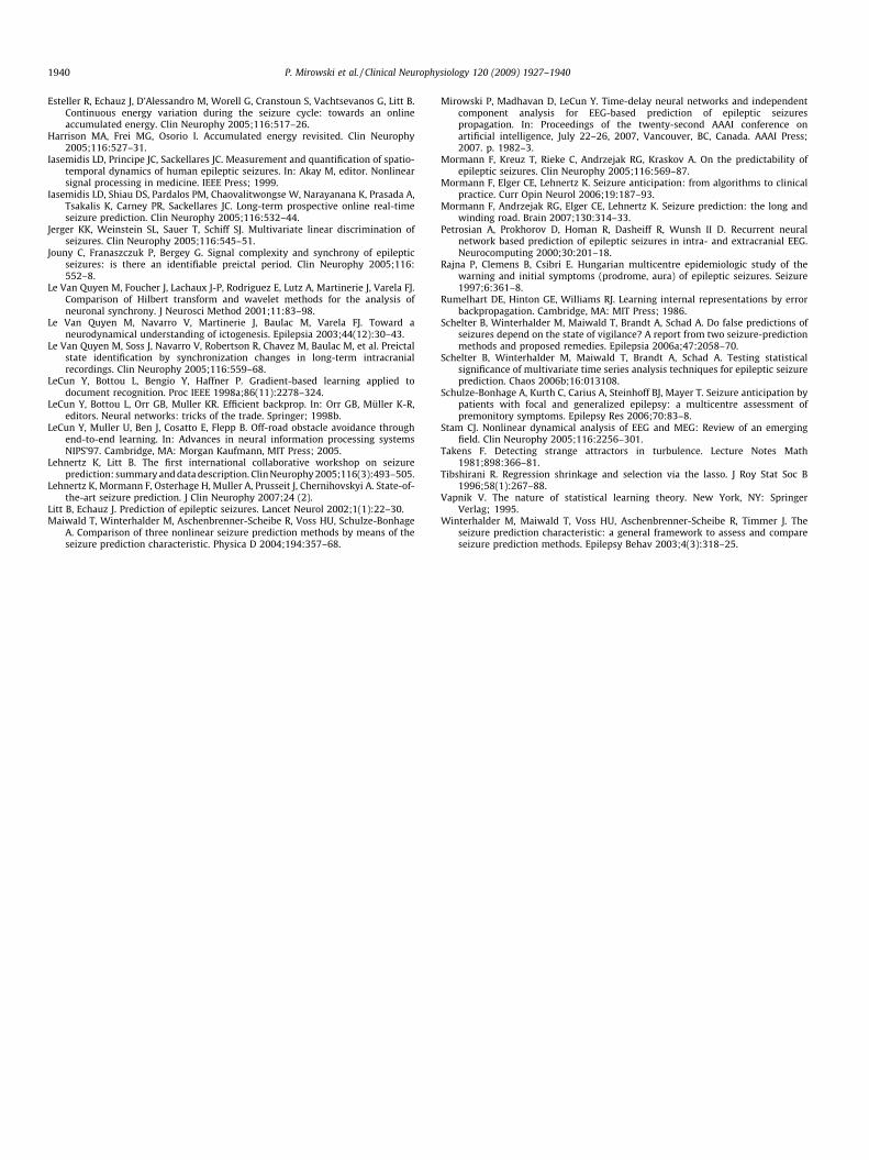
1940 P. Mirowski et al. / Clinical Neurophysiology 120 (2009) 1927–1940
Esteller R, Echauz J, D’Alessandro M, Worell G, Cranstoun S, Vachtsevanos G, Litt B.Continuous energy variation during the seizure cycle: towards an onlineaccumulated energy. Clin Neurophy 2005;116:517–26.
Harrison MA, Frei MG, Osorio I. Accumulated energy revisited. Clin Neurophy2005;116:527–31.
Iasemidis LD, Principe JC, Sackellares JC. Measurement and quantification of spatio-temporal dynamics of human epileptic seizures. In: Akay M, editor. Nonlinearsignal processing in medicine. IEEE Press; 1999.
Iasemidis LD, Shiau DS, Pardalos PM, Chaovalitwongse W, Narayanana K, Prasada A,Tsakalis K, Carney PR, Sackellares JC. Long-term prospective online real-timeseizure prediction. Clin Neurophy 2005;116:532–44.
Jerger KK, Weinstein SL, Sauer T, Schiff SJ. Multivariate linear discrimination ofseizures. Clin Neurophy 2005;116:545–51.
Jouny C, Franaszczuk P, Bergey G. Signal complexity and synchrony of epilepticseizures: is there an identifiable preictal period. Clin Neurophy 2005;116:552–8.
Le Van Quyen M, Foucher J, Lachaux J-P, Rodriguez E, Lutz A, Martinerie J, Varela FJ.Comparison of Hilbert transform and wavelet methods for the analysis ofneuronal synchrony. J Neurosci Method 2001;11:83–98.
Le Van Quyen M, Navarro V, Martinerie J, Baulac M, Varela FJ. Toward aneurodynamical understanding of ictogenesis. Epilepsia 2003;44(12):30–43.
Le Van Quyen M, Soss J, Navarro V, Robertson R, Chavez M, Baulac M, et al. Preictalstate identification by synchronization changes in long-term intracranialrecordings. Clin Neurophy 2005;116:559–68.
LeCun Y, Bottou L, Bengio Y, Haffner P. Gradient-based learning applied todocument recognition. Proc IEEE 1998a;86(11):2278–324.
LeCun Y, Bottou L, Orr GB, Muller KR. Efficient backprop. In: Orr GB, Müller K-R,editors. Neural networks: tricks of the trade. Springer; 1998b.
LeCun Y, Muller U, Ben J, Cosatto E, Flepp B. Off-road obstacle avoidance throughend-to-end learning. In: Advances in neural information processing systemsNIPS’97. Cambridge, MA: Morgan Kaufmann, MIT Press; 2005.
Lehnertz K, Litt B. The first international collaborative workshop on seizureprediction: summary and data description. Clin Neurophy 2005;116(3):493–505.
Lehnertz K, Mormann F, Osterhage H, Muller A, Prusseit J, Chernihovskyi A. State-of-the-art seizure prediction. J Clin Neurophy 2007;24 (2).
Litt B, Echauz J. Prediction of epileptic seizures. Lancet Neurol 2002;1(1):22–30.Maiwald T, Winterhalder M, Aschenbrenner-Scheibe R, Voss HU, Schulze-Bonhage
A. Comparison of three nonlinear seizure prediction methods by means of theseizure prediction characteristic. Physica D 2004;194:357–68.
Mirowski P, Madhavan D, LeCun Y. Time-delay neural networks and independentcomponent analysis for EEG-based prediction of epileptic seizurespropagation. In: Proceedings of the twenty-second AAAI conference onartificial intelligence, July 22–26, 2007, Vancouver, BC, Canada. AAAI Press;2007. p. 1982–3.
Mormann F, Kreuz T, Rieke C, Andrzejak RG, Kraskov A. On the predictability ofepileptic seizures. Clin Neurophy 2005;116:569–87.
Mormann F, Elger CE, Lehnertz K. Seizure anticipation: from algorithms to clinicalpractice. Curr Opin Neurol 2006;19:187–93.
Mormann F, Andrzejak RG, Elger CE, Lehnertz K. Seizure prediction: the long andwinding road. Brain 2007;130:314–33.
Petrosian A, Prokhorov D, Homan R, Dasheiff R, Wunsh II D. Recurrent neuralnetwork based prediction of epileptic seizures in intra- and extracranial EEG.Neurocomputing 2000;30:201–18.
Rajna P, Clemens B, Csibri E. Hungarian multicentre epidemiologic study of thewarning and initial symptoms (prodrome, aura) of epileptic seizures. Seizure1997;6:361–8.
Rumelhart DE, Hinton GE, Williams RJ. Learning internal representations by errorbackpropagation. Cambridge, MA: MIT Press; 1986.
Schelter B, Winterhalder M, Maiwald T, Brandt A, Schad A. Do false predictions ofseizures depend on the state of vigilance? A report from two seizure-predictionmethods and proposed remedies. Epilepsia 2006a;47:2058–70.
Schelter B, Winterhalder M, Maiwald T, Brandt A, Schad A. Testing statisticalsignificance of multivariate time series analysis techniques for epileptic seizureprediction. Chaos 2006b;16:013108.
Schulze-Bonhage A, Kurth C, Carius A, Steinhoff BJ, Mayer T. Seizure anticipation bypatients with focal and generalized epilepsy: a multicentre assessment ofpremonitory symptoms. Epilepsy Res 2006;70:83–8.
Stam CJ. Nonlinear dynamical analysis of EEG and MEG: Review of an emergingfield. Clin Neurophy 2005;116:2256–301.
Takens F. Detecting strange attractors in turbulence. Lecture Notes Math1981;898:366–81.
Tibshirani R. Regression shrinkage and selection via the lasso. J Roy Stat Soc B1996;58(1):267–88.
Vapnik V. The nature of statistical learning theory. New York, NY: SpringerVerlag; 1995.
Winterhalder M, Maiwald T, Voss HU, Aschenbrenner-Scheibe R, Timmer J. Theseizure prediction characteristic: a general framework to assess and compareseizure prediction methods. Epilepsy Behav 2003;4(3):318–25.


![An Optimal EEG-based Emotion Recognition Algorithm ......system based on EEG signals such as event-related synchronization [11] and event-related desynchronization [12]. A number of](https://static.fdocuments.net/doc/165x107/60591d1867969b0f56154721/an-optimal-eeg-based-emotion-recognition-algorithm-system-based-on-eeg-signals.jpg)