
Classification of Human Whole-Body Motion using … Conclusion 55. Page 1 1 Introduction Human...
70
KIT — University of the State of Baden-Wuerttemberg and National Research Center of the Helmholtz Association www.kit.edu Karlsruhe Institute of Technology Classification of Human Whole-Body Motion using Hidden Markov Models Bachelor’s Thesis of Matthias Plappert At the Department of Informatics Institute for Anthropomatics and Robotics (IAR) High Perfomance Humanoid Technologies Lab (H 2 T) Primary referee: Prof. Dr.-Ing. Tamim Asfour Secondary referee: Prof. Dr.-Ing. Rüdiger Dillmann Advisor: Dipl.-Inform. Christian Mandery Duration: May 1 st , 2015 – August 31 th , 2015
Transcript of Classification of Human Whole-Body Motion using … Conclusion 55. Page 1 1 Introduction Human...

KIT — University of the State of Baden-Wuerttemberg and National Research Center of the Helmholtz Association www.kit.edu
Karlsruhe Institute of Technology
Classification of Human Whole-Body
Motion using Hidden Markov Models
Bachelor’s Thesisof
Matthias Plappert
At the Department of InformaticsInstitute for Anthropomatics and Robotics (IAR)
High Perfomance Humanoid Technologies Lab (H2T)
Primary referee: Prof. Dr.-Ing. Tamim AsfourSecondary referee: Prof. Dr.-Ing. Rüdiger Dillmann
Advisor: Dipl.-Inform. Christian Mandery
Duration: May 1st, 2015 – August 31th, 2015
arX
iv:1
605.
0156
9v1
[cs
.LG
] 5
May
201
6


Erklärung:
Ich versichere hiermit, dass ich die Arbeit selbstständig verfasst habe, keine anderen als die angegebe-nen Quellen und Hilfsmittel benutzt habe, die wörtlich oder inhaltlich übernommenen Stellen als solchekenntlich gemacht habe und die Satzung des Karlsruher Instituts für Technologie zur Sicherung guterwissenschaftlicher Praxis beachtet habe.
Karlsruhe, den 31. August 2015
Matthias Plappert


Kurzzusammenfassung:
Diese Bachelorarbeit befasst sich mit der Klassifikation menschlicher Ganzkörperbewegung mittels Hid-den Markov Modellen (HMMs). Die menschlichen Bewegungen wurden mittels eines optisches Motion-Capture-Systems mit passiven Markern aufgenommen. Im Laufe der Arbeit werden zunächst Merk-male (features) erläutert, die die so aufgenommenen menschlichen Ganzkörperbewegungen beschrei-ben. Weiterhin wurden neue Merkmale aus den vorhandenen Rohdaten abgeleitet. Ein weiterer Schwer-punkt der Arbeit findet sich in der Diskussion von verschiedenen Ansätzen zur Lösung des Multi-Label-Klassifikationsproblems, also der Zuweisung von mehreren Klassen auf eine Bewegung. Hierbei wurdenzwei grundsätzliche Ansätze erarbeitet: Beim ersten Ansatz wird das Multi-Label-Problem zu einemMulti-Class-Problem transformiert, welches sich dann einfach lösen lässt. Der zweite Ansatz beschäftigtsich mit Möglichkeiten, das Multi-Label-Problem ohne vorhergehende Transformation zu lösen, indemdie Bewertungen einer unbekannten Bewegung durch die HMMs zu einer Gesamtvorhersage zusammen-gesetzt werden. Alle Aspekte des Klassifikators wurden anschließend auf einem aus 454 Bewegungenbestehenden Datensatz evaluiert. Hierbei wurden verschiedene Parameter und Konfigurationen vergli-chen. Weiterhin fand ein Vergleich zwischen HMMs und Factorial Hidden Markov Modellen (FHMMs)statt. Die zwei zuvor genannten Ansätze wurden in zwei verschiedenen Systemen realisiert und quanti-tativ miteinander verglichen. Hierbei erkannte das erste System 98,02% und das zweite System 93,39%der menschlichen Bewegungen auf dem Testdatensatz korrekt.


Contents
1 Introduction 1
2 Related Work 3
3 Basics 53.1 Motion Capture . . . . . . . . . . . . . . . . . . . . . . . . . . . . . . . . . . . . . . . 53.2 Master Motor Map . . . . . . . . . . . . . . . . . . . . . . . . . . . . . . . . . . . . . 63.3 KIT Whole-Body Human Motion Database . . . . . . . . . . . . . . . . . . . . . . . . 73.4 Hidden Markov Models . . . . . . . . . . . . . . . . . . . . . . . . . . . . . . . . . . . 83.5 Factorial Hidden Markov Models . . . . . . . . . . . . . . . . . . . . . . . . . . . . . . 11
4 Features 134.1 Marker Representation . . . . . . . . . . . . . . . . . . . . . . . . . . . . . . . . . . . 134.2 Joint Angle Representation . . . . . . . . . . . . . . . . . . . . . . . . . . . . . . . . . 144.3 Derived Features . . . . . . . . . . . . . . . . . . . . . . . . . . . . . . . . . . . . . . 164.4 Smoothing . . . . . . . . . . . . . . . . . . . . . . . . . . . . . . . . . . . . . . . . . . 184.5 Scaling . . . . . . . . . . . . . . . . . . . . . . . . . . . . . . . . . . . . . . . . . . . 18
5 Classification 215.1 Motion Recognition . . . . . . . . . . . . . . . . . . . . . . . . . . . . . . . . . . . . . 21
5.1.1 Emission Distribution . . . . . . . . . . . . . . . . . . . . . . . . . . . . . . . 215.1.2 Topologies . . . . . . . . . . . . . . . . . . . . . . . . . . . . . . . . . . . . . 215.1.3 Parameter Initialization . . . . . . . . . . . . . . . . . . . . . . . . . . . . . . . 225.1.4 Training and Recognition . . . . . . . . . . . . . . . . . . . . . . . . . . . . . . 235.1.5 Extension to Factorial Hidden Markov Models . . . . . . . . . . . . . . . . . . 23
5.2 Single-Label Classification . . . . . . . . . . . . . . . . . . . . . . . . . . . . . . . . . 255.3 Multi-Label Classification . . . . . . . . . . . . . . . . . . . . . . . . . . . . . . . . . 26
5.3.1 Power Set Method . . . . . . . . . . . . . . . . . . . . . . . . . . . . . . . . . 265.3.2 Binary Relevance Method . . . . . . . . . . . . . . . . . . . . . . . . . . . . . 275.3.3 Modified Algorithms . . . . . . . . . . . . . . . . . . . . . . . . . . . . . . . . 28
6 Evaluation 296.1 Tools . . . . . . . . . . . . . . . . . . . . . . . . . . . . . . . . . . . . . . . . . . . . . 29
6.1.1 dataset Module . . . . . . . . . . . . . . . . . . . . . . . . . . . . . . . . . 296.1.2 hmm Module . . . . . . . . . . . . . . . . . . . . . . . . . . . . . . . . . . . . 306.1.3 misc Module . . . . . . . . . . . . . . . . . . . . . . . . . . . . . . . . . . . 30
6.2 Dataset . . . . . . . . . . . . . . . . . . . . . . . . . . . . . . . . . . . . . . . . . . . 306.3 Feature Selection . . . . . . . . . . . . . . . . . . . . . . . . . . . . . . . . . . . . . . 336.4 Hidden Markov Models . . . . . . . . . . . . . . . . . . . . . . . . . . . . . . . . . . . 39
6.4.1 Hyperparameters . . . . . . . . . . . . . . . . . . . . . . . . . . . . . . . . . . 396.4.2 Parameter Initialization . . . . . . . . . . . . . . . . . . . . . . . . . . . . . . . 406.4.3 Factorial Hidden Markov Models . . . . . . . . . . . . . . . . . . . . . . . . . 42
6.5 Decision Makers . . . . . . . . . . . . . . . . . . . . . . . . . . . . . . . . . . . . . . 426.5.1 Logistic Regression . . . . . . . . . . . . . . . . . . . . . . . . . . . . . . . . . 446.5.2 Support Vector Machine . . . . . . . . . . . . . . . . . . . . . . . . . . . . . . 446.5.3 Decision Tree . . . . . . . . . . . . . . . . . . . . . . . . . . . . . . . . . . . . 46

6.5.4 Random Forest . . . . . . . . . . . . . . . . . . . . . . . . . . . . . . . . . . . 476.6 Classification Systems . . . . . . . . . . . . . . . . . . . . . . . . . . . . . . . . . . . 48
6.6.1 Power Set System . . . . . . . . . . . . . . . . . . . . . . . . . . . . . . . . . 496.6.2 Multi-Label System . . . . . . . . . . . . . . . . . . . . . . . . . . . . . . . . 526.6.3 Comparison . . . . . . . . . . . . . . . . . . . . . . . . . . . . . . . . . . . . . 53
7 Conclusion 55

Page 1
1 Introduction
Human whole-body motion plays an important role in many fields, including sports, medicine, entertain-ment, computer graphics and robotics. Motion capture technologies are readily available to relativelyeasily record vast amounts of data. Today, whole characters in movies and video games are created usingcomputer-generated imagery (CGI) and the recorded movements of an actor. An impressive exampleis the completely computer-generated character Gollum from the Lord of the Rings movies. In sportsand medicine, motion data can be used for gait analysis of humans. For example, stroke patients havebeen recorded using motion capture techniques to analyze their disease-induced walking disorders. Theinsights from this analysis can be used to better understand the symptoms of the patient and potentiallyallows the development of new rehabilitation therapies. Gait analysis is also used in professional sportsto analyze the performance of athletes and to optimize their training. In humanoid robotics, humanwhole-body motion plays an important role in the construction and control of biped humanoid robots.The use of motion in the field of robotics will be discussed in-depth in the Related Works chapter.
Given the interest in human motion and the availability of the recording equipment, a growing numberof motion data is recorded. A number of human whole-body motion databases exist today to makethis data available to artists, physicians and researchers. Retrieval of information from these databases isoften realized through so-called tags which are associated with a motion record. A motion can potentiallyhave many tags that describe it. For example, a motion of a human playing tennis might be labeled withthe tags tennis, forehand and right hand. These tags can be used to query the database for motion data ofinterest. However, annotating a motion with these tags is usually done by hand which is both an error-prone and slow process. The results are highly subjective since different annotators will use differenttags to label the same data. This may be because different annotators have a different understanding ofa tag or simply because they are not aware of the full set of available tags. Additionally, labeling everymotion by hand becomes infeasible as more data is recorded.
Autonomous motion recognition and classification can be used to automatically label new motionswithout human involvement. This approach solves the two main problems of labeling by hand. Firstly,the classification algorithm produces objective and reproducible results. Secondly, the system can bescaled to handle more and more data by increasing the available computational resources. The objectiveof this thesis is to develop a system that can be used to perform such autonomous classification of humanwhole-body motion.
This thesis is organized as follows: Chapter 2 provides a brief overview of the relevant literature andimportant authors in the field. Some fundamental concepts are introduced in chapter 3 which forms thebasis for all following chapters. This includes an in-depth discussion of motion capture systems and waysto represent this recorded data. The KIT Whole-Body Human Motion Database is introduced since thesystem developed during this thesis will be used to classify motions stored in this database. Additionally,the foundations of Hidden Markov Models (HMMs) and Factorial Hidden Markov Models (FHMMs)are discussed since they play a key role for the devised classifier. Chapter 4 discusses possible featuresto discriminate motions. The discussion includes different representations of motion data, the extractionof additional features from the data and important preprocessing steps before the features can be usedin a classifier. Chapter 5 is concerned with the problem of classification. In the chapter the previouslydiscussed basics of Hidden Markov Models are extended so that they can be used for motion recognition.The remainder of the chapter is devoted to the use of multiple HMMs for the classification of humanmotion. The theoretical concepts discussed in the previous chapters are then evaluated in chapter 6.Besides a description of the used tools and dataset, the evaluation includes the selection of features, acomparison between different HMM configurations as well as the evaluation of different classificationapproaches. Finally, the best results from each area are used to perform an end-to-end evaluation of theentire system. Chapter 7 summarizes the work and describes possible improvements for future work.
Classification of Human Whole-Body Motion using Hidden Markov Models


Page 3
2 Related Work
In robotics, a promising idea is to use human motion as an intuitive way to instruct and program machines.This approach is commonly referred to as Programming by Demonstration (PbD) [DRE+00, BCDS08].In PbD, a human instructor teaches a machine how to complete a given task by performing the necessarysteps themselves. The machine then observes the instructor and attempts to also complete the task byimitating what it perceives. Human motion can also be used to gain a better understanding of howdifferent parts of the human body work together to complete a task or goal. For example, observing howa human reacts to counter balance perturbations can potentially be used to transfer this knowledge tobiped humanoid robots [MBJA15, BPPŠ14]. Since motion plays a key role in humanoid robotics mostof the hereafter mentioned literature has a background in this area of research.
Different approaches exist for representing motions. Ogata et al. [OST05] used Recurrent NeuralNetworks (RNNs) for interactive learning. In their work, RNNs were used in a cooperative navigationtask with a humanoid robot and a human partner. Taylor et al. [THR06, TH09] proposed ConditionalRestricted Boltzmann Machines (CRBMs) to learn from and then generate human whole-body motion.The proposed model is capable of generating continuous motion sequences (e.g. walking) and alsoallows to smoothly transition between them by adding higher-order layers to the model. NonlinearOscillators were used by Nakanishi et al. [NME+04] in a framework for learning biped locomotion.Breazeal et al. [BBG+05] represented motion as a path through a directed weighted graph where eachnode represents a pose. The edges of the graph define transitions between poses that are physicallypossible and safe. Calinon et al. [CGB07] used a Mixture Model of Gaussian and Bernoulli distributions(GMM/BMM) to encode motion data. Yamane et al. [YYN09] represented continuous motions in binarytrees which can be used for motion recognition and generation. Lastly, Hidden Markov Models (HMMs)have been a popular choice to represent human whole-body motion. Since this work is concerned withHidden Markov Models, the following paragraphs review some works in this domain in greater detail.
Takano at al. [TYS+06] developed a system for recognizing and generating human motion for prim-itive nonverbal communication. Their approach uses a hierarchy of Hidden Markov Models for humanwhole-body motion recognition and motion generation. The lower layer represents motion primitives,also referred to as proto symbols, whereas the upper layer models the transitions between the motionprimitives and therefore represents higher-level interactions. The lower layer of the system was trainedon joint angle data recorded with an optical motion capture system. Multi-dimensional scaling was usedto construct a multi-dimensional space of proto symbols (the proto symbol space) on which the Hid-den Markov Model in the upper layer was trained. The authors evaluated their approach by recording akickboxing match between two humans. One of the human subjects was then replaced with a humanoidrobot. The model trained on the recorded data was used by the robot to generate and perform motions inresponse to the actions of its human counterpart.
Kulic et al. [KTN07b, KTN07a, KTN08] proposed a system for learning, clustering and hierarchy for-mation of human whole-body motion in humanoid robots. The authors used Hidden Markov Models andFactorial Hidden Markov Models to represent motion as a sequence of motion primitives. Additionally,the system described by the authors is capable of on-line learning. This was achieved by two essentialproperties of the devised system: sequential training of FHMMs and incremental hierarchical formationof the motion primitives by clustering. The sequential training algorithm allowed Kulic et al. to initiallyencode an observed motion into a simple Hidden Markov Model. As more and more data is observed,additional chains can be added and trained on-line, transforming the HMM into an FHMM. Secondly,newly observed motions are dynamically organized into an hierarchical tree structure, the motion symboltree. This can be done efficiently by performing a tree search and placing the new motion into the nodethat is most similar. Local clustering is performed to split groups into new subgroups as new knowledgeis added. As a result, specialized motions are placed at the leaves of the tree, whereas more generalized
Classification of Human Whole-Body Motion using Hidden Markov Models
Page 4 Chapter 2. Related Work
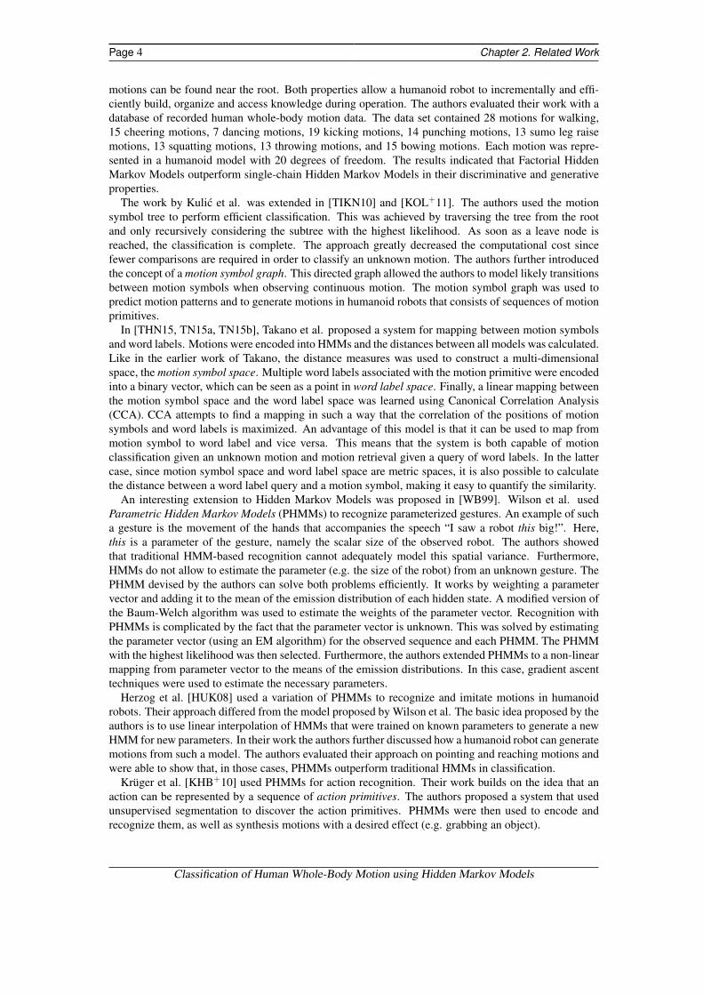
motions can be found near the root. Both properties allow a humanoid robot to incrementally and effi-ciently build, organize and access knowledge during operation. The authors evaluated their work with adatabase of recorded human whole-body motion data. The data set contained 28 motions for walking,15 cheering motions, 7 dancing motions, 19 kicking motions, 14 punching motions, 13 sumo leg raisemotions, 13 squatting motions, 13 throwing motions, and 15 bowing motions. Each motion was repre-sented in a humanoid model with 20 degrees of freedom. The results indicated that Factorial HiddenMarkov Models outperform single-chain Hidden Markov Models in their discriminative and generativeproperties.
The work by Kulic et al. was extended in [TIKN10] and [KOL+11]. The authors used the motionsymbol tree to perform efficient classification. This was achieved by traversing the tree from the rootand only recursively considering the subtree with the highest likelihood. As soon as a leave node isreached, the classification is complete. The approach greatly decreased the computational cost sincefewer comparisons are required in order to classify an unknown motion. The authors further introducedthe concept of a motion symbol graph. This directed graph allowed the authors to model likely transitionsbetween motion symbols when observing continuous motion. The motion symbol graph was used topredict motion patterns and to generate motions in humanoid robots that consists of sequences of motionprimitives.
In [THN15, TN15a, TN15b], Takano et al. proposed a system for mapping between motion symbolsand word labels. Motions were encoded into HMMs and the distances between all models was calculated.Like in the earlier work of Takano, the distance measures was used to construct a multi-dimensionalspace, the motion symbol space. Multiple word labels associated with the motion primitive were encodedinto a binary vector, which can be seen as a point in word label space. Finally, a linear mapping betweenthe motion symbol space and the word label space was learned using Canonical Correlation Analysis(CCA). CCA attempts to find a mapping in such a way that the correlation of the positions of motionsymbols and word labels is maximized. An advantage of this model is that it can be used to map frommotion symbol to word label and vice versa. This means that the system is both capable of motionclassification given an unknown motion and motion retrieval given a query of word labels. In the lattercase, since motion symbol space and word label space are metric spaces, it is also possible to calculatethe distance between a word label query and a motion symbol, making it easy to quantify the similarity.
An interesting extension to Hidden Markov Models was proposed in [WB99]. Wilson et al. usedParametric Hidden Markov Models (PHMMs) to recognize parameterized gestures. An example of sucha gesture is the movement of the hands that accompanies the speech “I saw a robot this big!”. Here,this is a parameter of the gesture, namely the scalar size of the observed robot. The authors showedthat traditional HMM-based recognition cannot adequately model this spatial variance. Furthermore,HMMs do not allow to estimate the parameter (e.g. the size of the robot) from an unknown gesture. ThePHMM devised by the authors can solve both problems efficiently. It works by weighting a parametervector and adding it to the mean of the emission distribution of each hidden state. A modified version ofthe Baum-Welch algorithm was used to estimate the weights of the parameter vector. Recognition withPHMMs is complicated by the fact that the parameter vector is unknown. This was solved by estimatingthe parameter vector (using an EM algorithm) for the observed sequence and each PHMM. The PHMMwith the highest likelihood was then selected. Furthermore, the authors extended PHMMs to a non-linearmapping from parameter vector to the means of the emission distributions. In this case, gradient ascenttechniques were used to estimate the necessary parameters.
Herzog et al. [HUK08] used a variation of PHMMs to recognize and imitate motions in humanoidrobots. Their approach differed from the model proposed by Wilson et al. The basic idea proposed by theauthors is to use linear interpolation of HMMs that were trained on known parameters to generate a newHMM for new parameters. In their work the authors further discussed how a humanoid robot can generatemotions from such a model. The authors evaluated their approach on pointing and reaching motions andwere able to show that, in those cases, PHMMs outperform traditional HMMs in classification.
Krüger et al. [KHB+10] used PHMMs for action recognition. Their work builds on the idea that anaction can be represented by a sequence of action primitives. The authors proposed a system that usedunsupervised segmentation to discover the action primitives. PHMMs were then used to encode andrecognize them, as well as synthesis motions with a desired effect (e.g. grabbing an object).
Classification of Human Whole-Body Motion using Hidden Markov Models

Page 5
3 Basics
Classification of human whole-body motion first and foremost requires motion data. This chapter there-fore starts with a brief discussion of motion capture (section 3.1) and the Master Motor Map as a frame-work for representing motion (section 3.2). Section 3.3 gives an overview of the KIT Whole-BodyHuman Motion Database, which plays an important role in this work since it stores all motion data andalso provides structures for labeling motions. Hidden Markov Models are introduced in section 3.4,which are used to learn and recognize motions in this work. Lastly, an extension of HMMs, FactorialHidden Markov Models, are discussed (section 3.5).
3.1 Motion Capture
For recording motion data, the VICON MX motion capture system can be used. The system uses passiveoptical markers that can be attached to both humans and objects. Cameras that are positioned at multiplelocations around the scene record the position of the markers within line of sight. To do so, each camerafeatures a ring of LEDs that surrounds its lens. The LEDs emit light in the infrared spectrum, whichis then reflected by the markers. Each camera records this reflected light and (depending on the modeof operation) reports the 2D coordinates of the markers. The final 3D coordinates for each marker arecalculated by triangulation using the data from each camera [vic].
Figure 3.1: Marker placement on the human body [MTD+15].
The motions are recorded by eight stationary and two portable VICON T10 cameras. Each camerarecords with a sampling rate of 100Hz. A total of 56 markers are placed onto the human as depicted infigure 3.1.
All recorded motion data is stored in the C3D format. The C3D format is a binary file format underpublic domain and is considered an industry standard. Besides storing marker coordinates in 3D space, it
Classification of Human Whole-Body Motion using Hidden Markov Models

Page 6 Chapter 3. Basics
also allows to store information about the human (e.g. body size and weight), the experiment setup (e.g.marker positions) as well as additional data (e.g. data from additional sensors like force sensors) [c3d].
3.2 Master Motor Map
Master Motor Map (MMM) [TUM+14, AAD07] is a framework for representation, mapping and repro-duction of human motions on humanoid robots. The fundamental goal of MMM is to map and unifydifferent motions performed by different humans and recorded with different motion capture systemsto the MMM reference model. Motions represented under this reference model can then be convertedto different outputs, e.g. to map a human motion onto a humanoid robot like ARMAR-III [ARA+06].The architecture of the MMM framework is depicted in figure 3.2. The framework includes differentcommand-line and graphical user interface (GUI) tools and is open source1.
RobotEditor
Master Motor Map
Reference Model
Motion Capturen
Converter n
dynamic dataforce data
...
MarkerlessMotion Capture1
Converter 1
object datahand poses
...
DataFormat
Marker‐based Motion Capture2
Converter 2
subject datajoint data
......
MotionDB
ConverterMMM ‐> RobotB
Robot B
ConverterMMM ‐> Visual.
Rendering
ConverterMMM ‐> AR
Action Recognition
ConverterMMM ‐> RobotA
Robot A
...ConverterMMM ‐> MA
Motion Analysis
Figure 3.2: Architecture of the Master Motor Map framework [TUM+14].
At the core of the framework is the MMM reference model. It consists of a model of the human bodywith a normalized height and weight, as well as kinematic and dynamic properties. These propertiesare based on the research conducted by Winter et al. [Win79, Win09] and Buchholz et al. [BAG92].The kinematics of the MMM model consist of 104 degrees of freedom (DoF): 6 DoF cover the modelpose, 23 DoF are assigned to each hand, and the remaining 52 DoF are distributed on arms, legs, head,eyes and body. The reference coordinate system in every joint is chosen in such a way that the x-axispoints to the right of the model, the y-axis to the front and the z-axis upwards. If a joint has multipleDoF it is split into multiple joints with a single DoF each. The MMM reference model also specifiesupper and lower limits for each joint. It is important to note that not all joints in the model must beused to represent motion. For example, the movement of individual fingers might not be of interest whenrecording a whole-body walking motion. In this case, the unspecified joints will simply remain in theirinitial positions [TUM+14].
The command-line tool MMMConverter can be used to convert data recorded with a motion capturesystem to the MMM reference model, i.e. reconstruct joint angles of the MMM model from motiondata. This is accomplished by placing virtual markers onto the reference model and finding a mappingfrom the position of the physical markers (as recorded by the motion capture system) to virtual markers.The optimization problem can be solved efficiently by minimizing the distance between the position of
1http://h2t.anthropomatik.kit.edu/752.php
Classification of Human Whole-Body Motion using Hidden Markov Models

Section 3.3: KIT Whole-Body Human Motion Database Page 7
physical and virtual markers for each frame. Details on this mapping procedure are given in [TUM+14].The converted motion is then stored in a XML-based file format. Such a XML file can contain multiplemotions, which is useful for scenes where a human interacts with objects or scenes with multiple humansin them. Each motion is referenced by a unique name and consists of two parts: a preamble and theactual motion data. The preamble specifies a model (e.g. the MMM reference model or a model of anobject) and can contain additional information about the human or object (e.g. body size and weight).The motion data is encoded in a list of frames. Each frame has a relative time step in seconds (the firstframe starts at time step t = 0) and contains values for all properties that are specified by the model.For example, each frame of human motion under the MMM reference model contains the root position(x, y, z coordinates), the root rotation (roll, pitch, yaw angles) and a list of joint angles. Additionally,the velocity and acceleration information for each of the above properties as well as dynamic data (e.g.center of mass, angular momentum) can be stored for each frame [mmm].
The GUI tool MMMViewer can be used to visualize motions. The whole motion can be played backor each frame can be inspected individually. The camera can be moved freely to view the motion fromdifferent angles. Additionally, the joint angles of the currently visible frame are displayed. Figure 3.3shows the tool during a visualization.
Figure 3.3: Visualization of a walking motion in MMMViewer.
3.3 KIT Whole-Body Human Motion Database
The KIT Whole-Body Human Motion Database2 contains motion data of both humans and objects thathave been recorded using a marker-based approach as described in section 3.1. Each entry in the databasehas a unique ID, belongs to a project, and references the subjects and objects that participated in therecording. When recording motions, multiple trials are usually performed. For each trial, the raw motiondata is stored in the C3D format (see section 3.1) and uploaded. Recorded data of additional sensors (e.g.force measurements for push recovery) as well as video footage can be uploaded as well. The databasesystem automatically converts the C3D files to a subject-independent representation under the MMMmodel (see section 3.2) and, optionally, estimates dynamic properties like the center of mass. Log filesgrant insight into the conversion process. Furthermore, the database is capable of storing data relatedto subjects and objects. Size, weight, gender and other anthropometric measurements can be stored in
2https://motion-database.humanoids.kit.edu
Classification of Human Whole-Body Motion using Hidden Markov Models

Page 8 Chapter 3. Basics
the record for each subject. For objects, a 3D model of the object alongside a custom description can besaved [MTD+15].
locomotion
bipedal
climb
...
manipulation
drop
pull
...
direction
forward
left
...
speed
fast
medium
slow
perturbation
result
source
gesticulation
bow
clap
...
sport
cartwheel
dance
...
walk
jump
...
failing
recovery
active
passive
(root)
Figure 3.4: The Motion Description Tree (excerpt) [MTD+15].
Each motion is classified within the Motion Description Tree. The tree consists of a hierarchical dec-laration of tags describing motion types (e.g. walk, kick, run) and additional tags for other properties likethe direction of a movement (e.g. left, right, forward, backward). The tree is organized in such a way thatthe parent of a node has a broader semantic meaning than its children. For example, the tags clap andbow are both child nodes of the tag gesticulation. An excerpt of the Motion Description Tree is depictedin figure 3.4. An important property of this classification approach is that a motion can be associatedwith an arbitrary number of nodes of the Motion Description Tree. For example, a motion of a humanthat trips while walking to the left with high speed can be categorized using the following tags: (1) loco-motion→ bipedal→ walk, (2) speed→ fast, (3) direction→ left, (4) perturbation→ result→ failing,and (5) perturbation→ source→ passive. The whole tree is managed by the KIT Whole-Body HumanMotion Database and can be extended if necessary [MTD+15].
The database can be accessed through a web interface or an application programming interface (API).The web interface and the API are available publicly. For each motion the raw files as well as theprocessed files can be downloaded. For convenience, bulk download options are available. The webinterface is also used to modify existing or upload new motions. These operations are restricted toregistered accounts. The API allows direct access to the database. This allows the integration of thedatabase into existing tools. The API is build on top of the Internet Communications Engine (Ice) [ice].Ice is a remote procedure call (RPC) framework and allows for easy integration with a wide variety ofplatforms and programming languages [MTD+15].
At the time of this writing, the database contains 4457 motions performed by 49 different subjects.All motions in total have a length of approximately 9 hours and 20 minutes, with the average length of arecording being approximately 7.56 seconds.
3.4 Hidden Markov Models
A Hidden Markov Model (HMM) [EAM08, Rab89] is a statistical model popular for learning sequentialdata. This is due to the fact that HMMs have the ability to have some degree of invariance to local warping(compression and stretching) of the time axis [B+06]. The methods discussed in this section are applica-ble to all forms of sequential data. However, since this work deals with temporal sequences, this sectionand all following chapters use notation and phrases that imply temporal sequences. Concretely, a tempo-
Classification of Human Whole-Body Motion using Hidden Markov Models

Section 3.4: Hidden Markov Models Page 9
ral sequence of length T is denoted by o1,o2, . . . ,oT , where each ot is a multi-dimensional observation.The following discussion of HMMs and the underlaying concepts are based on Bishop et al. [B+06].
ot−1 ot ot+1
Figure 3.5: Graphical representation of a first-order Markov chain. Each observation ot is only dependenton the previous observation [B+06].
To understand Hidden Markov Models, it is helpful to first consider a simpler Markov model: theMarkov chain. In a Markov chain (of first order), given a sequence o1, . . . ,oT , the conditional probabilityof an observation ot (that is the observation at time t) is assumed to be independent of all past (and, ofcourse, future) observations except for observation ot−1. The conditional distribution in a such a modelis given by
p(ot | o1, . . . ,ot−1) = p(ot | ot−1). (3.1)
Consequently, the joint distribution is given by
p(o1, . . . ,oT ) = p(o1)T
∏t=2
p(ot | ot−1). (3.2)
A graphical representation of a first-order Markov chain is depicted in figure 3.5. The assumption thatan observation is only dependent on its previous observation is rather strong. This can be easily seen byconsidering an example: If one attempts to predict the weather for the next hour by only considering thecurrent weather situation instead of using the data of the last 24 hours, the prediction would be severelylimited. The assumption can be relaxed by generalizing the Markov chain to be of M-th order. Here,each observation in a sequence is dependent on the past M observations. However, in such a model thenumber of parameters grows exponentially with M, so that this approach becomes impractical for largevalues of M.
zt−1 zt zt+1
ot−1 ot ot+1
Figure 3.6: Graphical representation of a Hidden Markov Model. Each observation ot (in blue) is condi-tioned on the state of its respective hidden variable zt (in red). The hidden variables form afirst-order Markov chain [B+06].
To solve this problem, hidden (sometimes also referred to as latent) variables are introduced. Con-cretely, each observation variable ot is conditioned on the state of its hidden variable zt . The hiddenvariables form a first-order Markov chain. Such a model is known as a state space model, which isvisualized in figure 3.6. The joint distribution for this model is given by
p(o1, . . . ,oT ,z1, . . . ,zT ) = p(z1)T
∏t=2
p(zt | zt−1)T
∏t=1
p(ot | zt). (3.3)
An important property of this model is that any pair of observed variables oi and o j are connected via thehidden variables. It can be shown that the predictive distribution p(ot+1 | o1, . . . ,ot) for observation ot+1is dependent on all past observations o1, . . . ,ot . This model is therefore not constrained by the strong
Classification of Human Whole-Body Motion using Hidden Markov Models

Page 10 Chapter 3. Basics
independence assumption of a Markov chain. If the hidden variables in a space state model as describedabove are discrete, the Hidden Markov Model is obtained.
Formally, a Hidden Markov Model is defined by the set of parameters that govern the model [B+06,Rab89]:
• K is the number of the individual hidden states. The appropriate number of states depends onthe problem at hand. The current state at time t is denoted by qt and the set of possible statesis S = {s1, . . . ,sK}. Notice the relationship of K and the hidden variables: Each of the K statesdescribes a possible value for the hidden variables zt . One way to represent this is through the1-of-K coding scheme, hence zt ∈ {0,1}K and ‖zt‖1 = 1 for each t. For example, the notationqt = s2 is equivalent to zt = (0,1,0, . . . ,0).
• A = (ai j) ∈ [0,1]K×K is a matrix that consists of transition probabilities. Concretely, each entrydefines the probability to transition to state s j given the current state si:
ai j = p(qt+1 = s j | qt = si). (3.4)
Since A is a probability distribution, it must hold that ∀ j : ∑k ak j = 1. By setting ai j = 0, it ispossible to “disable” that specific transition from si to s j.
• πππ = (π1, . . . ,πK) ∈ [0,1]K is the initial state distribution where
πi = p(q1 = si). (3.5)
It must hold that ‖πππ‖1 = 1.
• φ describes the parameters of the conditional distributions of the observed variables:
p(ot | zt ,φ). (3.6)
These probabilities are known as emission probabilities and can be given by different distribu-tions. For example, if the observed values are discrete, a conditional probability table can be used.For observations with continuous values, a Gaussian distribution is a often a good choice. Otherdistributions are possible and picking an appropriate distribution depends on the observations.
Since K is already encoded by the shape of A, an HMM is fully described by the following set ofparameters: θ = {A,πππ,φ}. In this work, an HMM with parameters θ is denoted by λθ .
Three fundamental problems can be identified when working with HMMs: (1) The evaluation prob-lem, (2) the decoding problem, and (3) the optimization problem. The problems and their description areall based on the work of Rabiner et al. [Rab89]. The first problem, the evaluation problem, is concernedwith calculating the probability of a given sequence under a given model. Formally, given a sequenceO = (o1, . . . ,oT ), how can p(O | λθ ) be calculated efficiently. This can also be viewed as scoring howwell a model matches the given observations. The forward-backward algorithm [BE+67, BS+68] canbe used to solve this problem (strictly speaking, only the forward pass is necessary to solve this firstproblem). The second problem, the decoding problem, is concerned with finding the state sequence ofthe hidden variables. Formally, given a sequence O = (o1, . . . ,oT ) and a model λθ , find a sequenceZ = (z1, . . . ,zT ) of hidden states that is optimal. Different criteria of an optimal state sequence exist, e.g.choosing the states that are individually most likely. The most popular criterion is to find the single beststate sequence. This is equivalent to maximizing p(Z |O,λθ ), which is solved efficiently by the Viterbialgorithm [Vit67]. The third problem, the optimization problem, is concerned with adjusting the param-eters of the model. Formally, given a sequence O = (o1, . . . ,oT ), find parameters θ such that p(O | λθ ) ismaximized. Solving this problem corresponds with learning the parameters, that is “training” the model.The Baum-Welch algorithm [BPSW70] solves this problem efficiently. However, since Baum-Welch isa specific case of the expectation maximization algorithm (EM algorithm), it does not necessarily find aglobal maximum.
Classification of Human Whole-Body Motion using Hidden Markov Models

Section 3.5: Factorial Hidden Markov Models Page 11
On a final note, another important property of HMMs is that they are generative models. This meansthat a model that has been trained on some data can be used to generate new samples. This is especiallyinteresting for human motions and humanoid robots. Here, a motion can be learned by observation andlater be reproduced in a robot by sampling from the model [TYS+06].
3.5 Factorial Hidden Markov Models
A sever limitation of HMMs is that they cannot represent a lot of information about the history of atime sequence. Factorial Hidden Markov Models (FHMMs) are a generalization of HMMs and offer away to overcome this limitation. For example, representing 30 bit of information about the history re-quires 230 hidden states in a standard HMM whereas an FHMM can represent the same information withonly 30 binary state variables [GJ97]. The discussion in this section is based on the work of Ghahra-mani et al. [GJ97].
z(1)t−1 z(1)t z(1)t+1
z(2)t−1 z(2)t z(2)t+1
z(3)t−1 z(3)t z(3)t+1
ot−1 ot ot+1
Figure 3.7: Graphical representation of a Factorial Hidden Markov Model. Each observation ot (in blue)is conditioned on the state of all its respective hidden variables z(1)t (in red), z(2)t (in green)and z(3)t (in purple). The hidden variables z(m)
t form a first-order Markov chain each. [GJ97].
In an FHMM, the current state is generalized by letting the state be represented by a collection of Mstate variables:
zt = (z(1)t , . . . ,z(M)), (3.7)
where each state variable z(m)t can take on K different values. Each state variable is constrained in such
a way that it evolves according to its own dynamics and is therefore uncoupled from the other statevariables:
p(zt | zt−1) =M
∏m=1
p(z(m)t | z(m)
t−1). (3.8)
This can be seen as M independent first-order Markov chains that all contribute to the observation. Thedistribution of the observed variable ot is conditional on the states of all hidden variables z(1)t , . . . ,z(M)
t foreach time step t. A simple way to represent this dependency for continuous observations is a multivariateGaussian. Concretely, given that each z(m)
t uses the 1-of-K coding scheme as described in section 3.4 and
Classification of Human Whole-Body Motion using Hidden Markov Models
Page 12 Chapter 3. Basics
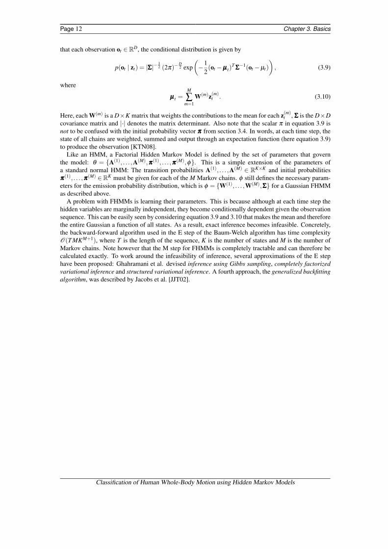
that each observation ot ∈ RD, the conditional distribution is given by
p(ot | zt) = |ΣΣΣ|−12 (2π)−
D2 exp
(−1
2(ot −µµµ t)
TΣΣΣ−1(ot −µt)
), (3.9)
where
µµµ t =M
∑m=1
W(m)z(m)t . (3.10)
Here, each W(m) is a D×K matrix that weights the contributions to the mean for each z(m)t , ΣΣΣ is the D×D
covariance matrix and |·| denotes the matrix determinant. Also note that the scalar π in equation 3.9 isnot to be confused with the initial probability vector πππ from section 3.4. In words, at each time step, thestate of all chains are weighted, summed and output through an expectation function (here equation 3.9)to produce the observation [KTN08].
Like an HMM, a Factorial Hidden Markov Model is defined by the set of parameters that governthe model: θ = {A(1), . . . ,A(M),πππ(1), . . . ,πππ(M),φ}. This is a simple extension of the parameters ofa standard normal HMM: The transition probabilities A(1), . . . ,A(M) ∈ RK×K and initial probabilitiesπππ(1), . . . ,πππ(M) ∈RK must be given for each of the M Markov chains. φ still defines the necessary param-eters for the emission probability distribution, which is φ = {W(1), . . . ,W(M),ΣΣΣ} for a Gaussian FHMMas described above.
A problem with FHMMs is learning their parameters. This is because although at each time step thehidden variables are marginally independent, they become conditionally dependent given the observationsequence. This can be easily seen by considering equation 3.9 and 3.10 that makes the mean and thereforethe entire Gaussian a function of all states. As a result, exact inference becomes infeasible. Concretely,the backward-forward algorithm used in the E step of the Baum-Welch algorithm has time complexityO(T MKM+1), where T is the length of the sequence, K is the number of states and M is the number ofMarkov chains. Note however that the M step for FHMMs is completely tractable and can therefore becalculated exactly. To work around the infeasibility of inference, several approximations of the E stephave been proposed: Ghahramani et al. devised inference using Gibbs sampling, completely factorizedvariational inference and structured variational inference. A fourth approach, the generalized backfittingalgorithm, was described by Jacobs et al. [JJT02].
Classification of Human Whole-Body Motion using Hidden Markov Models

Page 13
4 Features
As already mentioned in section 3.1, motions can be recorded using an optical marker-based motioncapture system. The following section discusses different approaches to represent such motions anddescribes possible features that are used to recognize and classify them in later chapters.
4.1 Marker Representation
A natural and obvious way to represent the recorded data is in 3-dimensional Cartesian space. For eachtime sample t, the system records the location of each marker n:
r(n)t = (x(n)t ,y(n)t ,z(n)t ) ∈ R3. (4.1)
A complete motion or observation sequence O is then represented by the all marker locations for allsampled time steps. A way to write this is to “unroll” all marker locations for a given time step t into thet-th row of an observation matrix:
Ocartesian =
x(1)1 y(1)1 z(1)1 . . . x(N)
1 y(N)1 z(N)
1
x(1)2 y(1)2 z(1)2 . . . x(N)2 y(N)
2 z(N)2
......
.... . .
......
...x(1)T y(1)T z(1)T . . . x(N)
T y(N)T z(N)
T
∈ RT×3N , (4.2)
where T is the number of time samples and N is the number of markers. A visualization of a motion andthe respective marker locations is depicted in figure 4.1.
Figure 4.1: Five key frames of a squatting motion with the location of the individual markers visualized.The subject looks to the left and is depicted from the side.
A problem with this representation is that an absolute coordinate system is used. Consider for exampletwo running motions. Assume that in the first case the subject moves towards a defined point and inthe second case turns 45 degrees and repeats the motion almost identically. However, since an absolutecoordinate system is used, the values in the observation matrix O will be very different for the two almostidentical motions. The same problem occurs if the start location of two motions is offset. Again, similarmotions will have different marker positions in the observation matrix. In short, the representation in anabsolute Cartesian coordinate system is neither invariant to translation nor rotation. A coordinate systemthat is relative to the recorded subject is desirable to allow for robust motion recognition.
Classification of Human Whole-Body Motion using Hidden Markov Models

Page 14 Chapter 4. Features
4.2 Joint Angle Representation
The Master Motor Map (MMM, [TUM+14]) framework (see also section 3.2) uses a relative coordinatesystem. This is achieved by mapping the position of the physical markers onto virtual markers on areference model. To do so, the squared error between the physical and virtual markers is minimizedby varying the pose of the subject (as defined by its position and rotation in space as well as its jointangles) while maintaining the constraints of the reference model. The optimization problem is solved bythe reimplementation of the Subplex algorithm as provided by the NLOpt library [MBJA15]. Figure 4.2depicts the kinematics and shows the location and labels of all joints.
Figure 4.2: The kinematics of the MMM reference model [TUM+14].
Some joints have multiple degrees of freedom (DoF). Take, for example, the body lower neck (BLN)joint that has 3 DoF (to convince yourself that this is indeed the case, nod, shake your head and move yourhead from shoulder to shoulder). In robotics, this is usually handled by splitting a joint with multipledegrees of freedom into multiple joints with a single DoF each. In the case of the exemplary BLNjoint, this means that the joints BLNx, BLNy and BLNz will replace it. After this step, each joint has asingle DoF and can therefore be represented as a scalar value that defines the joint angle in radians. Thecomplete joint configuration at time step t can therefore be written as
θθθ t = (θ(1)t ,θ
(2)t , . . . ,θ
(N)t ) ∈ RN , (4.3)
where N is the number of joints with a single DoF each. Similar to a representation in Cartesian space, a
Classification of Human Whole-Body Motion using Hidden Markov Models

Section 4.2: Joint Angle Representation Page 15
complete observation sequence can then be written as:
Ommm =
θ(1)1 θ
(2)1 . . . θ
(N)1
θ(1)2 θ
(2)2 . . . θ
(N)2
......
. . ....
θ(1)T θ
(2)T . . . θ
(N)T
∈ RT×N , (4.4)
where T denotes the number of time samples.It is important to stress again that the the joint angle representation is relative to the subject. However,
some important information is lost: the position of the subject in space. To overcome this, the absoluteroot position and the root rotation at each time step t are included in the MMM framework as well:
r(root)t = (xt ,yt ,zt) ∈ R3, (4.5)
θθθ(root)t = (θ
(roll)t ,θ
(pitch)t ,θ
(yaw)t ) ∈ R3. (4.6)
However, these properties are once again given in an absolute coordinate system, suffering from the sameproblem described above. Luckily, this is resolved easily by an affine transformation of the coordinatesystem translating it such that the root position at t = 0 starts at the origin and rotating it such that they axis points away from the front of the subject. The following two equations describe the necessarycalculations for each time step t:
∆r(root)t = r(root)
t − r(root)0 , (4.7)
r(root)t = R−1
∆r(root)t . (4.8)
The first equation describes the translation, whereas the second equation describes the rotation. A rotationmatrix for roll, pitch and yaw angles is given in [Cra05]:
R =
cosα cosβ cosα sinβ sinγ− sinα cosγ cosα sinβ cosγ + sinα sinγ
sinα cosβ sinα sinβ sinγ + cosα cosγ sinα sinβ cosγ− cosα sinγ
−sinβ cosβ sinγ cosβ cosγ
, (4.9)
where α := θ(yaw)0 , β := θ
(pitch)0 and γ := θ
(roll)0 .
Figure 4.3 plots the root position of two motions where the subject runs forward. The same movementsare depicted once before any normalization has been applied and once after normalization. Notice thatwithout normalization, the features are neither translation nor rotation invariant. This can be especiallywell seen in figure 4.3(a): Although the subject is running only forward, the movement is split betweenthe x and y components. This is because the subject moves at an approximately 45 degree angle betweenthe x and y axis of the absolute coordinate system. After normalization (figure 4.3(c)), the movementdirection happens only in the direction of the y axis of the transformed and now relative coordinatesystem. Hence rotation and translation invariant features are obtained after normalization.
The root rotation must be normalized as well to make it comparable. Since the rotation is given inangles, the normalization is straightforward:
θθθ(root)t = θθθ
(root)t −θθθ
(root)0 . (4.10)
Notice that this work assumes that the roll, pitch and yaw angles are not limited to the interval [−π,π].If necessary, this is easily achieved by correcting overflows by adding 2π to all following angles (andsimilarly subtracting 2π for underflows).
Another interesting usage of the MMM reference model is that it allows normalization of the markerpositions. Recall that the marker positions were previously given in an absolute coordinate system (seesection 4.1). However, since the initial pose of the subject is known in the MMM reference model, this
Classification of Human Whole-Body Motion using Hidden Markov Models

Page 16 Chapter 4. Features
0 50 100 150 200 250time steps
2500
2000
1500
1000
500
0
500
1000
1500
root
posi
tion
xyz
(a) The first running motion without normalization.
0 50 100 150 200 250 300 350time steps
2500
2000
1500
1000
500
0
500
1000
root
posi
tion
xyz
(b) The second running motion without normalization.
0 50 100 150 200 250time steps
500
0
500
1000
1500
2000
2500
3000
3500
4000
root
posi
tion
xyz
(c) The first running motion with normalization.
0 50 100 150 200 250 300 350time steps
500
0
500
1000
1500
2000
2500
3000
root
posi
tion
xyz
(d) The second running motion with normalization.
Figure 4.3: Comparison between the root positions of two different running motions before and afternormalization.
information can be used to normalize the marker positions as well. This is done analogously to thenormalization of the root position for the position of each marker (see equation 4.8).
4.3 Derived Features
Multiple additional features are computed under the MMM reference model. Firstly, an obvious exten-sion is to calculate the velocities and accelerations of all features that describe positions in Cartesiancoordinate space. Given that the velocity is the first derivative of the position and the acceleration isthe first derivative of the velocity, both properties are easily calculated by approximating the respectivederivatives:
vt =rt+1− rt−1
2∆tand at =
vt+1−vt−1
2∆t, (4.11)
where v denotes the velocity, a the acceleration and ∆t is the time difference between two subsequentsamples (which is assumed to be equidistant over all samples). The velocity and acceleration must benormalized as well. The normalization works similarly to equation 4.8 but normalizes each sample withthe current pose of the respective segment instead of normalizing each sample with the initial root pose.An interesting modification of the velocities and accelerations is to reduce them to simple scalar valuesby using their norm instead, e.g. the Euclidean one.
Secondly, since the MMM reference model provides additional information about the subject, moreadvanced features are computed as well. Two interesting dynamic properties are the center of mass
Classification of Human Whole-Body Motion using Hidden Markov Models

Section 4.3: Derived Features Page 17
0 50 100 150 200 250 300 350time steps
120
100
80
60
40
20
0
20
root
posi
tion
xyz
0 50 100 150 200 250 300 350time steps
200
150
100
50
0
50
100
150
cente
r of
mass
xyz
Figure 4.4: Comparison between the root position (left) and center of mass (right) of the same bowingmotion.
(CoM) and the angular momentum [PE04]. The CoM is conceptually similar to the root position dis-cussed earlier in the sense that it describes the position of a subject in 3-dimensional Cartesian space.However, while the root position is always at a fixed point on the reference model, the center of massis the barycenter of the subject. More concretely, the center of mass is the average over the CoM po-sitions of body segments weighted by their respective masses. To clarify this, consider a motion wherethe subject performs a deep bow. A bowing motion is interesting in this case since the lower body re-mains mostly fixed in space while the upper body moves down. Figure 4.4 plots the root position and theCoM of such a motion. Notice that the z component of the root position remains approximately constantalthough the upper body moves down during the bow. The z component of the CoM on the other handfirst decreases while the subject bows down and then increases again as the subject comes back up. Nowconsider the y component of the root position: It decreases as the subject bows down since the hip ofthe subject moves backwards. Compare this to the y component of the CoM that instead increases asthe subject bows down since that shifts the center of mass forward. Like the root position, the CoM isgiven in an absolute coordinate system. The normalization to a coordinate system relative to the subjectis done analogous to the normalization of the root position. The velocity and acceleration of the CoMare computed as well.
The angular momentum is a physical measure for the rotational configuration of an object or a systemin 3D space. In the MMM framework, the the angular momentum is calculated with respect to thecenter of mass at each time step t in all three spatial directions. The whole-body angular momentum iscalculated as follows:
Lt =M
∑i=1
(m(i)(r(i)t ×v(i)t )+ I(i)t ωωω
(i)t
)∈ R3, (4.12)
withr(i)t = r(CoMi)
t − r(CoM)t and v(i)t = r(CoMi)
t − r(CoM)t . (4.13)
The first part of the sum considers the angular momenta created by the orbital rotation of each segmentaround the whole-body center of mass. For each segment i ∈ {1, . . . ,M}, m(i) describes its mass, r(i)t itsposition at time step t w.r.t. the CoM and v(i)t its velocity at time step t w.r.t. the CoM. The cross productis denoted as ×. The second part of the sum takes the spin of each segment into account by computingthe product of its inertia tensor I(i)t and its angular velocity ωωω
(i)t . The velocity v(i)t and the difference in
CoM r(i)t must be normalized as previously described.Thirdly, the position of body segments are used as features as well. Consider for example a waving
motion. In this case, the positions of the hands are an interesting feature. Similarly, the position of thefeet are interesting for other motions, e.g. a kick. The positions of the extremities must be normalized.The velocities and accelerations are computed as previously described.
Classification of Human Whole-Body Motion using Hidden Markov Models

Page 18 Chapter 4. Features
4.4 Smoothing
The described features can be noisy or contain errors. For example, noise is introduced during the record-ing process. In addition, approximating the derivative for the computation of velocities and accelerationscan amplify errors and inaccuracies in the recorded data. Smoothing is used to reduce the impact of theseinterferences. A signal can be smoothed using a wide variety of different filters. For a more completediscussion, see [Sim12].
In this work, only a simple filter is briefly discussed: the moving average or sliding window filter. Insuch a filter of length W , the mean of the surrounding W data points is used instead of the individual datapoint:
xt =1
W +1
W/2
∑j=−W/2
xt+ j, (4.14)
where xt denotes a (potentially multi-dimensional) data point at time step t and x is the smoothed versionthereof. Including future samples into the average avoids introducing a time delay in the signal. Noticethat averaging over future samples is possible if the smoothing is applied off-line.
0 50 100 150 200 250 300 350time steps
20000
15000
10000
5000
0
5000
10000
15000
20000
root
acc
ele
rati
on
xyz
0 50 100 150 200 250 300 350time steps
20000
15000
10000
5000
0
5000
10000
15000
20000
root
acc
ele
rati
on
xyz
Figure 4.5: The components of a subject’s root acceleration during a running motion before (left) andafter (right) a moving average filter with W = 3 was applied.
Figure 4.5 compares the root acceleration of a subject before and after applying a moving average filter.Notice that the the original signal is very noisy. The smoothed signal maintains the overall structure ofthe signal but reduces the amount of jitter. Smoothing is a useful preprocessing step before feeding thefeatures into a model.
4.5 Scaling
Feature scaling is another preprocessing step. Take for example the joint angles and the root positionfrom the previous sections. The joint angles are physically constrained to a very narrow value range,whereas the root position can potentially grow very large if the subject travels a large distance from thestart position. It should be obvious from this example that features are on very different scales. Thisdifference in scale becomes a problem if k-means clustering is used to initialize an HMM’s emissiondistribution parameters. If the data is on very different scales across dimensions, k-means will not findclusters that properly fit the data because the same distance measure is minimized across dimensions.This, in turn, results in bad estimates of the emission distribution parameters which results in vanishingprobabilities and numerical instabilities during inference. To counter this, feature scaling is performed.A very simple but effective strategy is to scale the features such that each feature’s values are in the samerange, e.g. [−1,1]. This is achieved by applying the following equation to each individual feature x over
Classification of Human Whole-Body Motion using Hidden Markov Models

Section 4.5: Scaling Page 19
all T time steps:
xt = 2 ·xt − min
i∈{1,...,T}xi
maxi∈{1,...,T}
xi− mini∈{1,...,T}
xi−1. (4.15)
Notice that each feature needs to be scaled over all samples, not per-sample. Furthermore, if featurescaling is used, the computation of the minimum and maximum are computed on the training data. Newsamples (e.g. from the test dataset when evaluating or unknown motions when used productively) arethen simply scaled using the previously computed values. Otherwise the features that were used to trainthe model and the features that are used to recognize unknown motions would end up on a differentscales.
Classification of Human Whole-Body Motion using Hidden Markov Models


Page 21
5 Classification
This chapter discusses methods to recognize and classify motions represented by features as described inthe previous chapter. In the first section, the general concepts of Hidden Markov Models introduced inchapter 3.2 are concretely discussed for the case of motion recognition. In motion recognition, the goalis to encode a motion into a Hidden Markov Model and compute a measure that describes how likely anunknown motion is under the model. In the second section, motion recognition is extended to performmulti-class classification. In contrast to motion recognition, the goal is now to assign an unknown motionexactly one class out of a (potentially large) set of possible classes. Lastly, methods for performing multi-label classification are introduced. In contrast to the multi-class classification task, an unknown motioncan have many labels that assign it to multiple classes.
To avoid confusion and to emphasize the distinction between multi-class (where one label assigns eachmotion one class) and multi-label (where multiple labels assign each motion multiple classes), multi-classclassification is referred to as single-label classification hereinafter.
5.1 Motion Recognition
Hidden Markov Models are a popular choice for encoding human whole-body motions [TYS+06, KTN07a,KTN08]. This section describes some properties of HMMs in depth and discusses properties and prob-lems that are especially relevant when dealing with motions.
5.1.1 Emission Distribution
Recall that the emission distribution models the observed data. Since in this case motions are observed,and all previously discussed features are continuous, the emission distribution must also be continuous.Typically, a Gaussian distribution or a mixture model thereof is used to model this case [KTN08]. Sincethis work uses a multivariate Gaussian distribution, the following discussion focuses on this distribution.
A multivariate Gaussian or normal distribution is defined by two parameters, its mean vector µµµ ∈ RD
and its covariance matrix ΣΣΣ ∈ RD×D, where D is the dimension of the feature vector. The probabilitydensity function (pdf) is then given by
f (x) = |ΣΣΣ|−12 (2π)−
D2 exp
(−1
2(x−µµµ)T
ΣΣΣ−1(x−µµµ)
). (5.1)
In an HMM, the emission of each state k is governed by its mean vector µµµk and its covariance matrixΣΣΣk. When dealing with motions, the covariance matrices are often constrained to be diagonal to avoidnumerical problems [KTN07a, KTN07b].
5.1.2 Topologies
An important property of a Hidden Markov Models is that it uses hidden states. The transition probabil-ities between the K states are given by the transition matrix A ∈ [0,1]K×K , while πππ ∈ [0,1]K defines thestart probabilities for each state. By constraining the transition matrix (and as a result the start probabili-ties), different topologies can be realized. This is easily done by initializing the transition matrix and thestart probabilities with some entries set to zero. During training, all probabilities that were initially set tozero will remain at zero [Rab89].
If the transition matrix is not constrained, a transition from any given state to every other state canoccur. Such an HMM is usually referred to as fully connected or ergodic. Another popular topology
Classification of Human Whole-Body Motion using Hidden Markov Models

Page 22 Chapter 5. Classification
Figure 5.1: Illustration of a 4-state ergodic HMM (left) and a 4-state left-to-right HMM with with ∆ = 2(right) [Rab89].
is the left-to-right topology or Bakis topology [Bak76]. In such a topology, the states are thought to bealigned sequentially from left to right. At each state, only a transition to a state that is right of the currentstate or a self-transition is allowed. The model can thus only be traversed from left to right, hence thename. In a left-to-right model, the start probabilities are set to πππ = (1,0, . . . ,0) while the transition matrixtakes the following shape:
A =
a1,1 a1,2 . . . a1,(K−1) a1,K0 a2,2 . . . a2,(K−1) a2,K...
.... . .
......
0 0 . . . a(K−1),(K−1) a(K−1),K0 0 . . . 0 aK,K
. (5.2)
The left-to-right constraint can thus be written as:
ai, j = 0, j < i. (5.3)
To avoid skipping too many states while traversing from left to right, an additional constraint is intro-duced:
ai, j = 0, j > i+∆. (5.4)
∆ limits the maximum number of allowed skips [Rab89]. The left-to-right topology is frequently usedfor the recognition of motions [TYS+06, KTN07a]. Both, the ergodic and the left-to-right topology arevisualized in figure 5.1. Note that, due to the variate of possible constraints for the transition matrix,other topologies are possible which are not discussed here.
5.1.3 Parameter Initialization
An interesting problem that arises is how to initialize the values of the transition matrix and the startprobabilities as well as the means and covariance matrices of the emission distributions. Since theBaum-Welch algorithm does not necessarily converge to a global maximum but rather to a local one (seechapter 3.2), a proper initial estimate is important to increase the chances of finding the global maximumduring training. According to [Rab89], the start probabilities and transition matrix can either be initial-ized by a random (while maintaining the constraint that the respective probabilities must sum to one) oruniform estimation. Note that the constraints imposed by the topology choice must also be maintained.
The initialization of the mean vectors and covariance matrices of the emission distribution is morecomplicated. While a random initialization is possible, it is beneficial to perform an initial estimate ofthe underlaying distribution. A popular approach works as follows: The basic idea is to find K clustersthat correspond to the K states of the Hidden Markov Model. The mean µµµk and covariance matrix ΣΣΣk
Classification of Human Whole-Body Motion using Hidden Markov Models

Section 5.1: Motion Recognition Page 23
for each state k are then estimated over the respective k-th cluster [Rab89]. The necessary clustering canbe performed by hand. Alternatively an unsupervised clustering algorithm like the k-means algorithmcan be used to automatically cluster the data. The k-means algorithm works by alternately assigning datasamples to a cluster given the current parameters and then updating the cluster center means such that thedistance from the previously associated samples is minimized. Lloyd’s algorithm is often used to solvethe clustering problem efficiently [KMN+02].
5.1.4 Training and Recognition
After deciding on the hyperparameters of the model (namely the number of states, the topology andthe initialization method for the parameters of the model), the model can be trained. The training of anHMM is performed efficiently using the Baum-Welch algorithm [BPSW70]: For each training sequenceO the parameters of the model are updated by first computing the expected likelihood given the currentparameters (expectation step) and then updating the parameters such that the expected quantity fromthe expectation step is maximized (maximization step). When performed iteratively, the likelihood ismaximized. The E and M steps are repeated until convergence or until a fixed number of iterations havebeen performed.
A common problem when using the Baum-Welch algorithm are numerical instabilities. This is dueto the fact that the probabilities during the forward or backward pass can become extremely small sincethey are multiplied at each time step. This becomes worse as the sequences grow longer. Since motionsare usually at least a couple of hundred samples long, this becomes a very real problem when trainingHMMs on motions. The problem is mitigated by either using a scaling technique [Rab89] or by adaptingthe algorithm such that it uses the logarithm of the probabilities instead [Man06].
Another important property is that the training is unsupervised. This means that no target value like alabel is necessary to learn the parameters of the HMM. However, if multiple HMMs are used to classifymotions into classes, supervised learning becomes important. This will be discussed in the next section.Finally, HMMs can be trained off-line and on-line. In off-line training, the HMM is trained only once andthe parameters are kept fixed even if previously unseen observation sequences become available. Mostdiscussion in the literature assume off-line learning, e.g. [Rab89]. In on-line learning on the other hand,the HMMs are trained incrementally as new data becomes available. Kulic et al. [KOL+11] describesuch a system. This work only considers the off-line approach.
After the model has been trained, recognition is performed by calculating the likelihood under themodel λ for an unknown observation sequence O:
p(O | λ ). (5.5)
This is done efficiently by the forward algorithm [Rab89]. Since the forward algorithm is used duringtraining as well, the same underflow issues as discussed earlier apply. Notice that the likelihood canbecome larger than 1 by definition, hence 0≤ p(O | λ )< ∞. Since the likelihood can become both verysmall (that is, very close to zero but not negative) and very large, the logarithmic likelihood (loglikeli-hood) is usually computed and presented. A strongly positive loglikelihood thus indicates a motion thathas been strongly recognized by the model whereas a strongly negative loglikelihood indicates that themotion has not been recognized by the model at at. Finding such a decision boundary will be discussedlater in this chapter.
5.1.5 Extension to Factorial Hidden Markov Models
The previously discussed concepts apply equally to Factorial Hidden Markov Models. However, threeadditional considerations are of interest: the number of Markov chains as an additional hyperparameter,efficient training of the FHMM and computation of the likelihood under the model.
Firstly, the number of chains is an important hyperparameter since it directly controls the complexityof time series that an FHMM can represent. However it also comes at the cost of increasing the compu-tational complexity of both the training and the evaluation given an unknown observation sequence (see
Classification of Human Whole-Body Motion using Hidden Markov Models

Page 24 Chapter 5. Classification
chapter 3.5). In the literature, few chains are usually used. For example, Kulic et al. [KTN08] use onlytwo chains in their work. This does not seem like a lot at first. However, assume that an FHMM with15 states and 2 chains is used. This results in 152 = 225 possible state combinations. Compared to anHMM with 15 states, even such a relatively small FHMM can already represent vastly more history thanits HMM counterpart.
Exact training of FHMMs is computationally very expensive and can be, depending on the parameters,even infeasible. Four different approximations were already briefly discussed in chapter 3.5. However,Kulic et al.[KTN08] proposed a fifth approach that the authors used to train FHMMs on motion data.The authors further showed that their approach is at least as good as and in most cases even betterthan the exact inference algorithm when using it to train FHMMs on motion data. This makes theirapproach especially interesting for this work. The algorithm devised by the authors works as follows:The FHMM is trained sequentially. This means that each FHMM starts with a single chain. Inferenceis then performed using the standard Baum-Welch algorithm on the training data. For the next chain m,the residual error between the previously trained chains and the n-th training sample O(n) ∈ RT×D iscomputed for each time step t ∈ {1, . . . ,T}:
e(n)t =1
W
(o(n)t −
m−1
∑i=1
Wc(i)t
)∈ RD, (5.6)
where e(n)t is the residual error between the frame at time step t of the n-th training sample and thesummed contributions of the previous m−1 chains. Each chain’s contribution is weighted by W = 1/M,where M is the number of all chains. Finally, the contribution for each chain m at time step t is computedas follows:
c(m)t =
K
∑k=1
µµµ(m)k γ
(m)t,k ∈ RD, (5.7)
where K denotes the number of states, µµµ(m)k is the D-dimensional mean vector of the emission distribution
of the already trained chain m in state k. Furthermore, γ(m)t,k denotes the probability that state k in chain
m is active at time step t. Algorithm 1 summarizes the described training procedure.
initialize first chaintrain first chain on time series O(n) = (o(n)t ) using the Baum-Welch algorithmfor m = 2, . . . ,M do
initialize next chain mcompute residual errors e(n)1 , . . . ,e(n)T
train chain m on time series E(n) = (e(n)t ) using the Baum-Welch algorithmend
Algorithm 1: The sequential training algorithm for FHMMs in pseudo code [KTN08].
A noteworthy and convenient property of the sequential training algorithm is that it uses proceduresthat are already used when training HMMs. More concretely, the training of each chain is done by anunmodified version of the well-known Baum-Welch algorithm. Computing γ
(m)t,k for the residual error is
achieved just as easily by using the standard forward-backward algorithm.Lastly, the likelihoods under the FHMM must be calculated as well. This is done using the exact
algorithm given in [GJ97]. In the more concrete case of the sequential training algorithm, the necessarymeans and covariances are computed as follows:
µµµk1,...,kM=W
M
∑m=1
µµµ(m)km
and ΣΣΣk1,...,kM =W 2M
∑m=1
ΣΣΣ(m)km
. (5.8)
Classification of Human Whole-Body Motion using Hidden Markov Models

Section 5.2: Single-Label Classification Page 25
Notice that this must be done for each possible combination of states across all M chains, as indicatedby the index k1, . . . ,kM . Take, for example, an FHMM with 3 states and 2 chains. This would result in32 = 9 combinations, with the following mean vectors:
µµµ1,1 =W(
µµµ(1)1 +µµµ
(2)1
), µµµ1,2 =W
(µµµ(1)1 +µµµ
(2)2
), µµµ1,3 =W
(µµµ(1)1 +µµµ
(2)3
), (5.9)
µµµ2,1 =W(
µµµ(1)2 +µµµ
(2)1
), µµµ2,2 =W
(µµµ(1)2 +µµµ
(2)2
), µµµ2,3 =W
(µµµ(1)2 +µµµ
(2)3
), (5.10)
µµµ3,1 =W(
µµµ(1)3 +µµµ
(2)1
), µµµ3,2 =W
(µµµ(1)3 +µµµ
(2)2
), µµµ3,3 =W
(µµµ(1)3 +µµµ
(2)3
). (5.11)
The 9 covariance matrices would be calculated analogously. The emission distribution for each statecombination is then given by a multivariate Gaussian distribution with mean µµµk1,...,kM
and covarianceΣΣΣk1,...,kM [JJT02, KTN08].
5.2 Single-Label Classification
In the previous chapter motion recognition was discussed. This discussion is now extended to a classi-fication problem. In a classification problem an unknown observation sequence, in this case a motion,must be assigned to a finite set of classes L . For example, assume that the set of classes is run, jumpand kick. The goal is then to find the correct label y ∈L = {run, jump,kick} for an unknown motion Oby making a prediction p. The classification is correct if y = p. Figure 5.2 provides an overview of theclassification process. This process is used throughout this work, not just for single-label classification.
O . . .
λ2
λ1
λM−1
λM
. . .
p(O | λ2)
p(O | λ1)
p(O | λM−1)
p(O | λM)
Dec
isio
nM
aker
prediction
Figure 5.2: Overview of the classification process. For an unknown observation sequence O (in red),the likelihood under each HMM (in green) is computed. Each HMM corresponds to a singleclass. The likelihoods (in purple) are then fed into a decision maker (in orange) that computesthe prediction (in blue).
If only a single label is assigned to a motion, the classification is straightforward. Instead of usingwords, y is encoded by natural numbers where each number corresponds to a class:
y ∈ {1, . . . ,M}, (5.12)
where M is the number of classes that need to be recognized. The mapping between word and class
Classification of Human Whole-Body Motion using Hidden Markov Models

Page 26 Chapter 5. Classification
can be chosen arbitrarily as long as it is bijective. In the above example, a possible mapping would berun→ 1, jump→ 2 and kick→ 3.
Additionally, assume that M HMMs have been trained per class: λ1, . . . ,λM . The first HMM was onlytrained with motions of class 1, the second one only with motions of class 2 and so on. In contrast tothe learning algorithm described in the previous chapter, the labels of the training data are now used toselect the appropriate HMM during training. While the training of the HMM itself is still unsupervised,the selection happens in supervised fashion.
After training, the prediction of an unknown motion O must be computed. To do so, the likelihoods ofthe motion under each individual HMM are evaluated. The last step is then performed by what this workrefers to as a decision maker. The job of a decision maker is to find a mapping from the likelihoods ofthe HMMs to the prediction p. In case of the single-label classification problem, the prediction is doneby a very simple decision maker that chooses the label that corresponds to the HMM with the maximumlikelihood:
p = argmaxm∈{1,...,M}
p(O | λm). (5.13)
5.3 Multi-Label Classification
Let us now extend the classification problem to a problem where multiple labels can be assigned to amotion. This can be motivated by recalling the Motion Description Tree (see chapter 3.3): A motionis specified by the leave nodes of the tree, e.g. (1) locomotion → bipedal → walk, (2) speed → fast,(3) direction→ left, (4) perturbation→ result→ failing, and (5) perturbation→ source→ passive. Itshould be obvious from this example that most motions cannot be adequately described by a single class.However, if a motion can have multiple labels, the simple classification described by equation 5.13 doesnot work anymore since it only computes the single label with the maximum likelihood.
To work around this problem, two different approaches can be identified: problem transformationusing the power set method or the use of more advanced decision makers. In the latter case, the decisionmaker needs to truly handle multi-label classification. This can either be done by using the binaryrelevance method or algorithm modification [RPHF11].
5.3.1 Power Set Method
A first attempt to solve this problem is to simply treat each possible combination of labels as a singleclass. More formally, if L is the set of all labels, compute the power set as the substitute label set:
L = P(L ) = {U |U ⊆L }\ /0. (5.14)
If each element in L is then mapped to a natural number, the multi-label problem has been transformedinto a single-label problem. This means that equation 5.13 can be used to predict the substitute labelwith the maximum likelihood. Since the substitute label represents multiple labels internally, reversingthe transformation after the classification step solves the multi-label problem using the already discussedapproach for single-label classification. In the literature, this idea is usually referred to as the power-setmethod [BLSB04, RPHF11].
The power set method, however, has several downsides. Firstly, the number of possible label combi-nations is 2M−1, where M is the number of classes. Recall that for each class a Hidden Markov Modelmust be trained. However, having sufficient training data now becomes a problem. If, for example, 200walking motions exist but of those 200 motions only a single a has the labels walk and fast whereasall others have the labels walk and slow, the HMM for the fast walking motion would only be trainedon a single training sample. This is inefficient since the HMM would benefit from the samples of thesimilar slow walking motion. Secondly, to perform classification, the likelihood under each model mustbe calculated. It can be easily seen that, for the worst case, this requires O(2M) computations of theloglikelihood for each unknown motion, which makes this approach infeasible for even moderately largeM.
Classification of Human Whole-Body Motion using Hidden Markov Models

Section 5.3: Multi-Label Classification Page 27
5.3.2 Binary Relevance Method
Instead of treating all possible combinations of labels as a single label, an approach where a motion cantruly have multiple labels is interesting. One way to achieve this is to encode the label as a binary vector:
y ∈ {0,1}M, (5.15)
where ym is set to 1 if the m-th label is active and set to 0 otherwise. To give an explanatory example,assume that the classes walk, fast and slow exist. The label of a fast walking motion would then beencoded as y = (1,1,0) whereas motion where the subject walks slowly would would be encoded asy = (1,0,1).
The training then works as follows: M HMMs are initialized, one for each class. Given a trainingsequence O, use it to train all HMMs which correspond to the set classes in the sequence’s label y. If, forexample, y = (1,0,1), train λ1 and λ3 on the same sequence. An advantage over the previously describedmethod is that only M instead of 2M − 1 HMMs (worst case) must be kept in memory. Additionally,the utilization of the available training data is vastly improved. In the above example, the HMM thatcorresponds to the walk class now benefits from both, the slow and fast walks. In the previously describedapproach, both would only be considered in isolation. However, this can also become a problem if classesare too generic. Take for example motion of a throw performed with the left hand and a kick with theleft foot. If both would be associated with the same class left, it is unlikely that common patterns canbe learned properly. Instead, hand-left and foot-left can be used to distinguish the two, which is a morereasonable choice in this case.
However, it is unclear how the decision maker can be realized in this case. The previous approachwhere the class with the maximum likelihood was selected cannot be used anymore. One way to per-form classification in this case is to use some fixed value as the decision boundary. Let xm be such adecision boundary for the m-th label. The multi-label classification is then achieved by computing alllikelihoods of the unknown motion O under each HMM and selecting all that are equal to or greater thanthe respective decision boundary:
pm =
{1, if p(O | λm)≥ xm
0, otherwisem = 1, . . . ,M, (5.16)
where ym denotes the m-th element of the prediction p. This approach is promising, but unfortunately itall depends on a good choices of xm.
Instead of trying to find good values for all xm by hand, it would be preferable if the decision boundariescould be determined automatically. Since the approach described in this work is supervised, the asso-ciation between the likelihoods and the corresponding class is actually known for the training dataset.It seems like a good idea to use this knowledge to learn a decision boundary from the training data in-stead of finding it by hand. This has the advantage that the model easily adapts to the current datasetat hand without the need to fine-tune the decision boundary manually. The problem can indeed be seenas binary classification: For each class, the features for the binary classifier are the likelihoods whichshould be classified into two half-spaces that correspond to the labels 0 and 1 respectively. Since in thiscase, the feature space is 1-dimensional (just a scalar likelihood under one specific model), the hyper-plane that separates the two half-spaces is a simple point and corresponds to the decision boundary xmdescribed previously. This means that any binary classifier like Logistic Regression [Jor02] or SupportVector Machines [HDO+98] can be used to learn a mapping from the likelihoods to ym for each class.
Instead of only considering the m-th likelihood, in a slightly more advanced version of this basicidea the binary classifier considers all likelihoods for its binary decision. This approach is commonlyreferred to as the binary relevance method [RPHF11]. More concretely, multi-label motion classificationis realized with this method as follows:
Classification of Human Whole-Body Motion using Hidden Markov Models

Page 28 Chapter 5. Classification
1. Given the training data O(1), . . . ,O(N) and respective labels y(1), . . . ,y(M), calculate the likelihoodsfor each motion under each model:
x(n) = (p(O(n) | λ1), p(O(n) | λ2), . . . , p(O(n) | λM)), n ∈ {1, . . . ,N}. (5.17)
2. Train M binary classifiers. For each classifier, the features are x(1), . . . ,x(N). However, the labelsare varied across classifiers, with the m-th classifier using labels y(1)m , . . . ,y(N)
m .
3. Given an unknown motion O, calculate the likelihoods x under each of the M models analogouslyto equation 5.17. Afterwards, perform M predictions using the previously trained classifiers toobtain the complete multi-label prediction:
p = (h(1)(x), . . . ,h(M)(x)), (5.18)
where h(m)(x) ∈ {0,1} denotes a function that computes the prediction of the m-th classifier.In this case, the decision maker uses multiple binary classifiers internally to learn a mapping from the
likelihoods of the HMMs to the multi-label prediction using the binary relevance method. It is importantto stress again that the ability to use any binary classifier for multi-label predictions is a big advantage ofthis method since a wide and well-understood variety of such classifiers exist.
However, this approach also has a downside: Each class is considered in isolation. This means thatinformation is lost since the correlation between classes in the label vector y carries information aswell. More concretely, it is likely that certain label combinations correspond to certain patterns in thelikelihoods. Such patterns cannot be detected by the approach described above, since each classifier only“sees” a single class [RPHF11].
5.3.3 Modified Algorithms
Some learning algorithms have been modified to support multi-label classification “out of the box”. Insuch a case, the multi-label classification is straightforward: Similarly to the previous approaches, thelikelihoods under each model are calculated for each of the N training motions and the likelihood vectorsx(1), . . . ,x(N) are obtained (compare equation 5.17). In contrast to the binary relevance method, theclassifier can now be trained on the entire label vector y instead of training individual classifiers on theindividual classes. This potentially allows the learning algorithm to find patterns between the likelihoodsand the classes since the correlation between classes can now also be considered. In this case the decisionmaker is thus simply a classifier that is capable of learning multi-label classification.
Multiple algorithms exist that have been adopted to the multi-label problem. Decision Trees havebeen extended to work in multi-label classification problems [VSS+08]. With this extension, RandomForests [Bre01] can also be used to perform multi-label classification since a Random Forest is an en-semble classifier that uses multiple Decision Trees internally. While this work focuses on the mentionedalgorithms, it should be noted that other algorithms have been modified as well to support multi-labelpredictions, e.g. AdaBoost [SS00] or k-Nearest Neighbors [ZZ07].
Classification of Human Whole-Body Motion using Hidden Markov Models

Page 29
6 Evaluation
The evaluation of the previously discussed concepts is challenging. This is due to the fact that a hugenumber of system parameters can be identified: A set of features must be selected, the hyperparametersof the Hidden Markov Models must be chosen, a comparison between FHMMs and HMMs is neces-sary and a variety of different classifiers that perform the mapping from likelihoods to final labels areavailable which also potentially have many hyperparameters that need fine-tuning. It should be clear thatevaluating all those DoFs simultaneously is impossible due to the large number of combinations. Instead,the problem is split into smaller problems that are evaluated and optimized individually. Only a smallsubset of the best parameter choices is then used in the next problem, and so on.
The structure of this chapter is based on this idea: To get started, a brief overview of the tools usedand developed for this work is given. The next section describes the used evaluation dataset. For the firstevaluation step, feature selection is performed to find a “good” subset of the wide variety of availablefeatures (see chapter 4). Next, Hidden Markov Models and their set of hyperparameters are evaluated (seechapter 5.1). The discussion is continued by a comparison between Hidden Markov Models and FactorialHidden Markov Models (see chapter 5.1.5). Different approaches to predict the labels are evaluated (seechapter 5.3). Finally, an end-to-end evaluation of two classifier systems is conducted using the resultsfrom the previous sections.
6.1 Tools
A toolkit was developed to help to evaluate this work. The toolkit is mostly written in Python with somemodules using C and C++ either for speed or for interoperability. Additionally, the excellent scikit-learnframework [PVG+11] was used throughout the toolkit. The toolkit is used via multiple command-linescripts. This allows to easily automate long-running tasks and handles the wide variety of differentactions and parameters efficiently. Areas of responsibility are split into 3 main modules which are eachbriefly covered in the remainder of this section.
6.1.1 dataset Module
The dataset module provides classes and functions to load motion from different file formats (MMMand C3D files). Furthermore, the derived features described in chapter 4.3 can be computed as well.The functionality of the Simox1 and MMMTools2 libraries are used to aid in the computation of moreadvanced features like the angular momentum. SWIG3 is used to bridge between Python and the C++API of the two mentioned libraries4,5. The module also provides functionality to normalize features toobtain rotation and translation invariant representations. Features can also be smoothed by applying amoving average filter and transformed to have similar scales across features. In short, the datasetmodule implements everything that was discussed in chapter 4.
Another important responsibility of the dataset module is the handling of datasets. A dataset isdefined by a simple manifest. The manifest is realized as a JSON file that contains an array of folders.Each folder can be label with multiple classes to perform supervised learning. A dataset can be loadedfrom such a JSON manifest file. Multiple file formats (MMM and C3D) can be merged into a combined
1http://simox.sourceforge.net2https://gitlab.com/mastermotormap/mmmtools3http://swig.org4https://gitlab.com/cmandery/pySimox5https://gitlab.com/cmandery/pyMMM
Classification of Human Whole-Body Motion using Hidden Markov Models

Page 30 Chapter 6. Evaluation
dataset. A dataset can be checked for inconsistencies (e.g. missing files), a report can be generated (e.g.the number of samples and the labels present in the dataset), selected features can be plotted to visualizethe data and the entire dataset can be exported into a single file (different file formats are supported).Especially the export functionality is important since the computation of the derived features and thenormalization is computationally expensive. All evaluation steps therefore load such an exported datasetinstead of computing the dataset from scratch every time.
Lastly, the dataset module also provides functionality that helps with splitting the dataset into twoseparate (and disjunct) datasets: one for training, one for testing. This is done using stratified k-foldfor multi-label data as proposed by Sechidis et al. [STV11]. The basic idea of a k-fold evaluation is tosplit the dataset into k disjunct subsets or folds. k rounds can then be performed by using k− 1 foldsfor training and the remaining fold for testing. In a stratified k-fold, each fold attempts to have the samedistribution of data across classes as the entire dataset.
6.1.2 hmm Module
The hmm module implements everything necessary to train and evaluate Hidden Markov Models. Thebasic HMM functionality is provided by the hmmlearn library6. Other libraries were considered aswell, namely pomegranate7 and GHMM8. However, hmmlearn proved to be the most reliable and fastestlibrary.
For this evaluation, a fork9 of the hmmlearn library was created and used. It fixes some issues and,more importantly, implements functionality to use and train Factorial Hidden Markov Models. The im-plementation allows to compute exact likelihoods as described by Ghahramani et al. [GJ97]. Addition-ally, it supports the sequential training algorithm developed by Kulic et al. [KTN08] (see chapter 5.1.5)
The module also provides functionality to combine the individual HMMs into an ensemble of HMMs.It allows training of the individual HMMs on labeled training data as well as computing the loglikeli-hoods of unknown motions under each model (see chapter 5.2 and 5.3). The training and evaluation oflikelihoods is performed in parallel for each model to maximize performance.
Lastly, the hmm module provides utility functions to compute the initial transition matrix and startprobabilities using different topologies (see chapter 5.1.2). Functions to estimate the initial means andcovariance matrices using different strategies and constraints as described in chapter 5.1.3 are includedas well.
6.1.3 misc Module
The misc module is a collection of smaller components. The most important one are the decisionmakers. A decision maker is a classifier that performs the mapping from the likelihoods as calculated bythe HMM ensemble to the binary label vector. As described in chapter 5.3, different approaches exist.The misc module implements a decision maker that always picks the maximum likelihood (chapter 5.2)and one that uses a fixed decision boundary (chapter 5.3.2). Additionally, decision makers that useLogistic Regression and Support Vector Machines are implemented using the binary relevance method(chapter 5.3.2). Decision Trees and Random Forests are used with adapted learning algorithms to handlethe multi-label problem directly (chapter 5.3.3). The decision makers make especially heavy use of thescikit-learn framework.
6.2 Dataset
Each motion in the dataset was recorded using the motion capture system described in chapter 3.1. Theraw positions of the motion markers were stored in a C3D file. Each motion was recorded using the KIT
6https://github.com/hmmlearn/hmmlearn7https://github.com/jmschrei/pomegranate8http://ghmm.org9https://github.com/matthiasplappert/hmmlearn
Classification of Human Whole-Body Motion using Hidden Markov Models

Section 6.2: Dataset Page 31
reference marker set consistent of 56 markers placed at well-defined anatomical locations and a samplingrate of 100Hz. The C3D files are converted to the MMM reference model using 40 joints (each with asingle DoF) and a non-linear optimization algorithm (see chapter 3.2). The joint angles as well as theroot position and root rotation were stored in an XML file. The C3D and XML files are used to extractand compute all features described in chapter 4. For all features, the normalized or unnormalized formcan be used. During normalization, the root rotation of the first frame was constrained such that the rolland pitch angles were set to zero. This is because a small error in either of the two angles can causean improperly rotated coordinate system. The features can also be smoothed using a moving averagefilter with W = 3 (compare chapter 4.4). Table 6.1 lists all 29 available features without differentiatingbetween normalized/unnormalized and smoothed/not smoothed.
Dimension Feature Name Description
40 joint_pos angles of all 40 joints40 joint_vel velocities of each joint
1 joint_vel_norm Euclidean norm of the joint velocities40 joint_acc acceleration of each joint
1 joint_acc_norm combined Euclidean norm of the joint accelera-tions
3 root_pos root position of the subject in Cartesian space3 root_vel directed root velocity1 root_vel_norm Euclidean norm of the root velocity3 root_acc directed root acceleration1 root_acc_norm Euclidean norm of the directed root acceleration3 root_rot pitch, roll and yawn angles of the subject’s root1 root_rot_norm Euclidean norm of the root rotation
12 extremities_pos position of the hands and feet in Cartesian space12 extremities_vel directed velocities of the hands and feet
4 extremities_vel_norm Euclidean norm of the directed extremity veloci-ties per hand/foot
12 extremities_acc directed accelerations of the hands and feet4 extremities_acc_norm Euclidean norm of the directed extremity veloci-
ties per hand/foot3 com_pos position of the center of mass in Cartesian space3 com_vel directed velocity of the center of mass1 com_vel_norm Euclidean norm of the CoM’s velocity3 com_acc directed acceleration of the center of mass1 com_acc_norm Euclidean norm of the CoM’s acceleration3 angular_momentum whole-body angular momentum in x, y and z di-
rection1 angular_momentum_norm Euclidean norm of the whole-body angular mo-
mentum168 marker_pos position of all 56 markers in Cartesian space168 marker_vel directed velocities of all markers
1 marker_vel_norm Euclidean norm of all markers’ velocities168 marker_acc directed acceleration of all markers
1 marker_acc_norm Euclidean norm of all markers’ accelerations
Table 6.1: List of all 29 available features with a total of 702 dimensions.
Classification of Human Whole-Body Motion using Hidden Markov Models

Page 32 Chapter 6. Evaluation
A total of 454 motions were selected from the motion database. 10 different human subjects performedthe motions. Of those 10 subjects, 3 are female and 7 are male. Each motion was performed by a singlehuman subject. If a motion involves an object (e.g. playing the guitar), the object was not physicallypresent but instead imagined by the subject. The only exception to this is a set of upwards walkingmotions where actual stairs were used since it is quite hard to climb imaginary ones. Each recording inthe dataset contains only a single motion. Additionally, each subject begins the motion in an upward-standing pose similar to the zero-pose of the MMM model and finishes the motion in the same pose. Forperiodic motions such as walking, stirring or dancing, a fixed number of repetitions were selected acrossthe dataset. The motions in the dataset were manually labeled with 49 different labels. Table 6.2 lists alllabels and the number of samples in the dataset that are assigned to each label. Since motions can havemultiple labels, table 6.3 lists all label combinations that are present in the evaluation dataset.
Motions Attributes
Samples Label Samples Label
180 walk 31 turn-right35 push-recovery 28 turn-left41 run 9 speed-fast28 kick 10 speed-normal10 throw 10 speed-slow10 bow 84 direction-forward
5 squat 14 direction-backward10 punch 15 direction-left10 stomp 12 direction-right25 jump 15 direction-upward11 golf 35 direction-circle20 tennis 27 direction-slalom15 wave 10 bend-right11 play-guitar 10 bend-left10 play-violin 18 counter-clockwise11 stir 17 clockwise11 wipe 23 foot-right11 dance 15 foot-left
45 hand-right48 hand-left5 hand-both5 deep5 slight
10 high10 low5 putting6 drive
10 smash10 forehand6 waltz5 chachacha
Table 6.2: List of all 49 different labels used in the dataset.
Classification of Human Whole-Body Motion using Hidden Markov Models

Section 6.3: Feature Selection Page 33
Samples Label Combination Samples Label Combination
10 walk, direction-forward, speed-normal 5 stomp, foot-right10 walk, direction-forward, speed-slow 5 stomp, foot-left
9 walk, direction-forward, speed-fast 5 jump, direction-forward31 walk, turn-right 5 jump, direction-backward28 walk, turn-left 5 jump, direction-right10 walk, bend-left 5 jump, direction-upward10 walk, bend-right 5 jump, direction-left18 walk, direction-circle, counter-clockwise 5 golf, putting17 walk, direction-circle, clockwise 6 golf, drive27 walk, direction-slalom 5 tennis, hand-right, smash10 walk, direction-upward 5 tennis, hand-right, forehand
9 push-recovery, direction-forward 5 tennis, hand-left, smash9 push-recovery, direction-backward 5 tennis, hand-left, forehand7 push-recovery, direction-right 5 wave, hand-right
10 push-recovery, direction-left 5 wave, hand-left41 run, direction-forward 5 wave, hand-both
8 kick, foot-right 5 play-guitar, hand-right5 kick, foot-right, high 6 play-guitar, hand-left5 kick, foot-right, low 5 play-violin, hand-right5 kick, foot-left, high 5 play-violin, hand-left5 kick, foot-left, low 5 stir, hand-right5 throw, hand-right 6 stir, hand-left5 throw, hand-left 5 wipe, hand-right5 bow, deep 6 wipe, hand-left5 bow, slight 6 dance, waltz5 squat 5 dance, chachacha5 punch, hand-right5 punch, hand-left
Table 6.3: All 54 label combinations used in the dataset.
6.3 Feature Selection
In feature selection, the goal is to find a subset of features that are relevant to the problem at hand. Theselection process is a crucial first step. This is due to the fact that any classifier can only compute pre-dictions from the features it receives. If those features do not contain the relevant features, the classifierobviously cannot produce optimal results. Additionally, a reduction of the feature dimensionality hasseveral advantages: Firstly, the computational complexity is usually proportional to the dimensionalityof the feature space. Secondly, if the feature space has very high dimensionality but the dataset is rela-tively small, overfitting becomes more likely. Lastly, reducing the feature set can also bring interestinginsights to better understand a problem at hand [GE03].
Unfortunately, the optimal feature set cannot be computed directly by evaluating all possible subsets.This is due to the fact that, for a feature set with N different features, 2N − 1 non-empty subsets exist.
Classification of Human Whole-Body Motion using Hidden Markov Models

Page 34 Chapter 6. Evaluation
As previously described, a set of N = 29 different features can be identified in this work with resultsin 229− 1 = 536870911 subsets. Evaluating each of these subsets is infeasible. In the literature, threepopular heuristics can be identified to solve this problem: the filter method, the wrapper method andthe embedded method. The filter method selects features by ranking them with correlation coefficients.The wrapper method evaluates the usefulness of a subset using a classifier. The embedded method workssimilarly to the wrapper method in the sense that it uses a predictor. However, while the wrapper methodsrelies on an external measure to assess the quality of the feature set, the embedded method relies onfeature selection that is inherent to the learning algorithms. To give a concrete example, Support VectorMachines with L1 regularization can be used to perform feature selection using the embedded method.This is possible because L1 regularization yields sparse weights. The selection can then be done bysimply picking all features that correspond to non-zero weights without the need of an externally definedmeasure [GE03].
In this work, feature selection is performed using the wrapper method with backwards elimination. Inbackwards elimination, one starts with the full feature set. Each feature is temporarily excluded fromthe set once and a model is trained on each of the subsets. For each subset, the model is evaluated onthe test set and a measure is computed. The feature with the least effect on the measure is then removedfrom the feature set. This process is repeated until the feature set is empty (or until a stopping criterionis reached). The feature selection was performed on the dataset described in section 6.2. Of the 29 avail-able features, the features marker_pos, marker_vel and marker_acc were initially excluded. This is dueto the very high dimensionality of the three mentioned features (168 dimensions each) that resulted innumerical problems. The three excluded features will be revisited later. Additionally, to avoid too muchcomplexity, all features under consideration were normalized, smoothed (using the previously describedmoving average with W = 3) and scaled to be in range [−1,1]. The reasoning behind this decision is thatit seems very unlikely that unnormalized features perform well since they are, as previously discussed,neither invariant to translation nor rotation. Another concern was that the unnormalized features cancause overfitting. The smoothed features were selected as the default for similar reasons since it seemsunlikely that an error-prone signal with strong jitter performs better than a slightly smoothed representa-tion thereof. Scaling is important to ensure a good initialization when using k-means clustering. Sincethe dataset contains 49 different classes, 49 HMM models with 5 states each and the left-to-right topol-ogy with ∆ = 1 were used. Each model was trained using the Baum-Welch algorithm for 10 iterations.The transition matrix and start probabilities were initialized uniformly whereas k-means clustering wasused to initialize the means and covariance matrices. The covariance matrix was further constrained to bediagonal and the diagonal elements were constrained to be larger than 0.0001 to avoid numerical instabil-ities. The entire dataset was initially shuffled to break correlations between nearby training samples. Astratified 3-fold was used to train and evaluate the HMMs three times per feature subset. In each round,the likelihoods under each model were calculated for the test split. The likelihoods were additionally splitinto a set of positive and negative likelihoods. The positive set contains all likelihoods of the motions thatshould have been recognized by the respective model whereas the negative set contains the likelihoodsof the motions that should have been rejected. Since 49 different HMMs are used this results in 98 setsof likelihoods: 49 sets of positive instances and 49 sets of negative instances. The mean and standarddeviation were then calculated per set over all three rounds, resulting in 98 means of the likelihoods andtheir respective standard deviations.
A possible way to measure the results in each round is to compute the distance between the distributionof positive and negative likelihoods on a per-class basis. The Wasserstein metric [GS+84, was] can beused to compute the distance between two Gaussian distributions:
mi =
√|µposi − µnegi |+
(σ2
posi+ σ2
negi−2√
σ2posi
σ2negi
), (6.1)
where i denotes the i-th class, µposi is the mean over all positive and µnegi the mean over all negativelikelihoods for the i-th class. σposi and σnegi denote the respective standard deviations. It was furtherassumed that the positive and negative likelihood distributions are Gaussian. This assumption is notformally proven here but seems likely to hold given the central limit theorem.
Classification of Human Whole-Body Motion using Hidden Markov Models
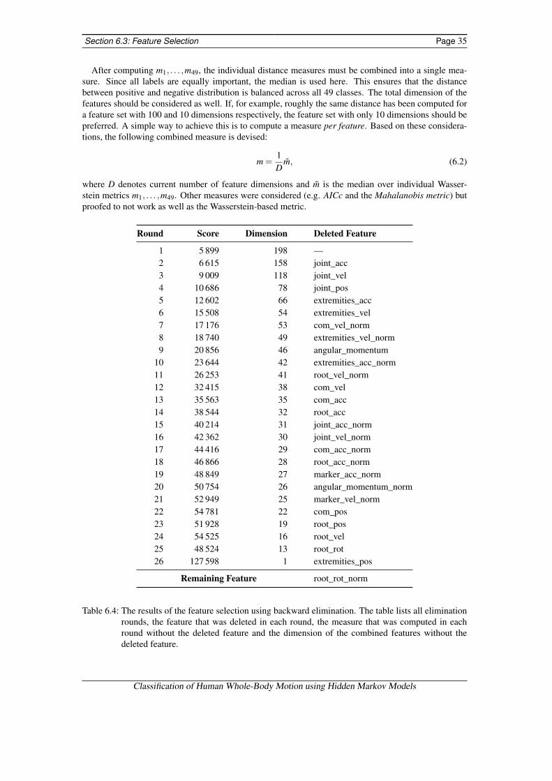
Section 6.3: Feature Selection Page 35
After computing m1, . . . ,m49, the individual distance measures must be combined into a single mea-sure. Since all labels are equally important, the median is used here. This ensures that the distancebetween positive and negative distribution is balanced across all 49 classes. The total dimension of thefeatures should be considered as well. If, for example, roughly the same distance has been computed fora feature set with 100 and 10 dimensions respectively, the feature set with only 10 dimensions should bepreferred. A simple way to achieve this is to compute a measure per feature. Based on these considera-tions, the following combined measure is devised:
m =1D
m, (6.2)
where D denotes current number of feature dimensions and m is the median over individual Wasser-stein metrics m1, . . . ,m49. Other measures were considered (e.g. AICc and the Mahalanobis metric) butproofed to not work as well as the Wasserstein-based metric.
Round Score Dimension Deleted Feature
1 5 899 198 —2 6 615 158 joint_acc3 9 009 118 joint_vel4 10 686 78 joint_pos5 12 602 66 extremities_acc6 15 508 54 extremities_vel7 17 176 53 com_vel_norm8 18 740 49 extremities_vel_norm9 20 856 46 angular_momentum
10 23 644 42 extremities_acc_norm11 26 253 41 root_vel_norm12 32 415 38 com_vel13 35 563 35 com_acc14 38 544 32 root_acc15 40 214 31 joint_acc_norm16 42 362 30 joint_vel_norm17 44 416 29 com_acc_norm18 46 866 28 root_acc_norm19 48 849 27 marker_acc_norm20 50 754 26 angular_momentum_norm21 52 949 25 marker_vel_norm22 54 781 22 com_pos23 51 928 19 root_pos24 54 525 16 root_vel25 48 524 13 root_rot26 127 598 1 extremities_pos
Remaining Feature root_rot_norm
Table 6.4: The results of the feature selection using backward elimination. The table lists all eliminationrounds, the feature that was deleted in each round, the measure that was computed in eachround without the deleted feature and the dimension of the combined features without thedeleted feature.
Classification of Human Whole-Body Motion using Hidden Markov Models

Page 36 Chapter 6. Evaluation
Table 6.4 lists the results per elimination round. The best feature was found in the last round: root_rot_norm.However, the individual likelihoods reveal that the single feature does not capture enough information torecognize all motion types. For example, the stir motion had a mean loglikelihood of −12046±43080,which clearly indicates that this motion cannot be recognized using only the normalized norm of the rootrotation. Some direction labels achieve similarly bad results. The label clockwise and counter-clockwisefor example achieved a loglikelihood score of −311± 67 and −275± 103 respectively. However, themean loglikelihoods for motions that should not be recognized by the models are 401±701 and 405±725respectively. This feature set was therefore discarded as an outlier.
The second best result was achieved in round 22 with the following set of features: root_pos, root_vel,extremities_pos, root_rot and root_rot_norm. This is a more reasonable result. The velocity of thesubject’s root certainly is important to detect the direction the subject moves in and to decide if themotion is of stationary or dynamic nature. The position of the extremities proved to be an especiallyimportant feature since it survived all elimination rounds until the last one. This also makes sense: Alot of motions in the dataset involve the subject’s hands or feet. Examples are stirring, waving, throwinga ball, playing the guitar or violin and kicks. The position of the extremities presumably also helpwith identifying which hand or foot was used to perform the motion. Including the root rotation andits norm makes sense as well: Since the root position and the root rotation are both included, it shouldbe possible to adequately determine the subject’s position and rotation in space from the feature set.This is obviously important information. An interesting observation is that the joint angles are not thatimportant to recognize motions. The joint angles were already discarded in the fourth round. This ispresumably due to the relatively low information contents per feature. While some joints might carryimportant information, this information is also redundantly present in other features like the position ofthe extremities. Since other feature sets achieved similar scores, they will be revisited in the last sectionduring the end-to-end evaluation.
All things considered, the selected features seem like a good choice. This claim is backed by thedata in table 6.6 (at the very end of this section) which lists the mean likelihoods and their standarddeviation per label over the entire test dataset for HMMs that were trained using the previously mentionedfeature set from elimination round 22. The likelihoods of positive samples are consistently high with areasonable standard deviation. Additionally, the models only respond to the motions that they weretrained to recognize. The only exception is the model that represents walking motions, which seemslikely to produce false positives. This is presumably due to the fact that very different walking motions(e.g. walking and making a 90 degree turn vs. walking forward) were used to train the same model. Thehigh standard deviation of the negative likelihoods can be explained by the fact that an extremely widevariety of very different motions were all combined into a single score. In other words: The positivelikelihoods were only computed for motions of the same type whereas the negative likelihoods combinesmotion of all other types into a single score.
Score Dimension Additional Feature
54 781 22 —
4 456 181 marker_pos
4 459 181 marker_vel
NaN 181 marker_acc
Table 6.5: Comparison between the baseline feature set and the previously excluded features. Each ofthe previously excluded features is added once to the baseline set and the performance isevaluated.
Recall that three features were excluded from the previous feature selection process: marker_pos,marker_vel and marker_acc. This was necessary because of numerical problems when including thesefeatures in the initial feature set during backwards elimination. More concretely, the probabilities during
Classification of Human Whole-Body Motion using Hidden Markov Models

Section 6.3: Feature Selection Page 37
inference would become so small that an underflow occurred even though the HMM implementationused during the evaluation already uses logarithmic probabilities to counter the problem. However, thesefeatures are now revisited. To do so, the best feature set as previously determined was used as a baseline.Each of the three left out features was then added once. The achieved scores (using the same measureand training procedure as before) are listed in table 6.5.
It is quite obvious from the data that the marker positions, velocities and accelerations do not contributeanything to the feature set; instead the scores worsen significantly. Notice that the marker accelerationseven cause numerical instabilities due to vanishing probabilities, hence a score cannot be computed in thiscase. The three temporarily excluded features are thus excluded permanently from further consideration.
Classification of Human Whole-Body Motion using Hidden Markov Models

Page 38 Chapter 6. Evaluation
Class Positive Loglikelihood Negative Loglikelihood
walk 12858±4924 10095±16747push-recovery 84073±26271 −830206±1314193run 13655±3937 −161784±344406kick 24898±5235 −207653±422938throw 25122±6796 −4982845±8584547bow 31251±4014 −5946674±9198336squat 32149±6640 −2198971±3600540punch 35073±11606 −1828241±3125022stomp 34982±3633 −3409349±5592487jump 24124±6256 −293847±612549golf 37559±8758 −1880819±3414369tennis 34408±3933 −303574±551566wave 58801±7035 −14784535±21892345play-guitar 49155±4275 −3531256±6955093play-violin 55510±3780 −6878584±10443505stir 28269±52856 −5574138±8338055wipe 48898±4734 −8223779±13225863dance 33981±5709 −178554±259631turn-right 18467±3158 −58574±111112turn-left 18594±7066 −36449±69685speed-fast 20673±3640 −333766±531406speed-normal 27002±8508 −393349±618222speed-slow 28689±2372 −410014±559746direction-forward 20472±17043 −159039±328429direction-backward 54408±24864 −720136±1467702direction-left 86904±52238 −949005±1478147direction-right 50982±24431 −1271632±1879763direction-upward 27477±4773 −194048±366744direction-circle 17183±6479 −24067±75746direction-slalom 23776±4992 −38560±106968bend-right 28950±3030 −191518±237383bend-left 23457±4346 −206328±262216counter-clockwise 21281±5297 −50763±115171clockwise 20271±8250 −45160±83697foot-right 25384±5914 −229056±472367foot-left 31525±2765 −1583832±2753615hand-right 39043±11234 −457165±819820hand-left 40720±11209 −380057±723547hand-both 62305±4304 −8376056±12155675deep 29047±2347 −5173123±7942443slight 31561±6827 −3272445±6239772high 29758±4651 −1173850±2088698low 27388±3102 −1653420±2928772putting 39531±4220 −4056969±6825540drive 36932±11987 −1846573±3369606smash 35313±4018 −328343±665057forehand 31963±4084 −826177±1417883waltz 36618±10136 −396325±634596chachacha 29362±8173 −797359±1213353
Table 6.6: The mean positive and negative loglikelihoods under each of the 49 classes for the feature setselected during round 22.
Classification of Human Whole-Body Motion using Hidden Markov Models

Section 6.4: Hidden Markov Models Page 39
6.4 Hidden Markov Models
As discussed in chapter 5.1, Hidden Markov Models can be used to perform motion recognition. How-ever, HMMs have multiple hyperparameters that need to be selected, namely the number of states andthe topology. Additionally, different initialization strategies can be used. As mentioned in chapter 5.1.3,proper initialization is a crucial step before training. Moreover, a comparison between the performanceof HMMs and FHMMs makes sense. FHMMs have another important hyperparameter, the number ofchains.
Throughout this section, the experimental setup from the previous feature selection section was usedagain. More concretely, the same dataset was used. To make the results comparable between this andthe previous section, the same permutation was used to shuffle the dataset. 3-fold cross-validation wasused with 49 HMMs, one for each class. Each HMM was trained for 10 iterations. The best feature setfrom the previous section was used throughout the following experiments: root_pos, root_vel, extrem-ities_pos, root_rot and root_rot_norm. All features were normalized, smoothed and scaled. The sameWasserstein-based metric (equation 6.2) from the previous chapter was used to score the results. Thedefault parameters of the HMMs were as follows: 5 states, left-to-right topology with ∆ = 1, uniforminitialization of the transition & start probabilities and k-means initialization of the Gaussian emissiondistribution parameters with the covariance matrices constrained to be diagonal. Notice that these areonly defaults. Each experiment will vary either one or multiple of these parameters, which will beclearly stated in each subsection.
6.4.1 Hyperparameters
The optimal number of states and topology are found using grid search. In grid search, each possiblecombination of hyperparameters is used to train a model on the training dataset which is then evaluatedon the test dataset. A measure is computed per combination and the best combination is selected. Sucha search is feasible in this case since only two different hyperparameters are evaluated.
In theory any natural number can be used for the number of states and countless different topologies arepossible. In practice however, it makes sense to limit the number of states K to be between 5 and 20 stateswhen recognizing human motions [KTN07a, KTN08]. In this evaluation K ∈ {3, . . . ,20}, resulting in18 different values for the number of states. The topologies (chapter 5.1.2) under consideration are thefollowing:
• fully-connected,
• left-to-right without a ∆ constraint,
• left-to-right with ∆ = 1, and
• left-to-right with ∆ = 2.
The left-to-right topologies proved to be especially well-suited for motion recognition [KTN08]. Dif-ferent variations of this topology are evaluated by varying the ∆ parameter. For completeness, the fully-connected topology is considered as well.
Hence 18 different values for the number of states and 4 different topologies were under evaluation.This results in a total of 18 · 4 = 72 combinations, making the grid search easily feasible. The previouslydescribed experimental setup was used, with all parameters fixed and set to their default values exceptfor the number of states and the topology. The results are depicted in figure 6.1.
As can be seen from the results, it is indeed desirable to have a low number of states. Good choices arebetween 5 and 8 states, depending on the topology. Another interesting observation is that the left-to-righttopology with ∆ = 1 is the only topology that performed consistently without large jumps. However, thebest result was achieved by the left-to-right topology without a ∆ constraint and with 8 states. The resultsupport the claim that a low number of states is preferable for motion recognition and that the left-to-righttopology is a good choice when dealing with motions. However, except for a few cases, the performanceacross topologies was similar.
Classification of Human Whole-Body Motion using Hidden Markov Models

Page 40 Chapter 6. Evaluation
3 4 5 6 7 8 9 10 11 12 13 14 15 16 17 18 19 20
number of states
25000
30000
35000
40000
45000
50000
55000
60000
scor
e
fully-connectedleft-to-right without ∆ constraintleft-to-right with ∆ = 1
left-to-right with ∆ = 2
Figure 6.1: The results of the hyperparameter grid search. The four different topologies are plotted indi-vidually. For each topology the number of states are plotted against the respectively achievedscore.
6.4.2 Parameter Initialization
Different strategies can be used to initialize the parameters of a Hidden Markov Model before startingthe training (see chapter 5.1.3). To quickly recap, the transition matrix and the start probabilities caneither be initialized uniformly or by randomization. The implementation of a uniform initialization istrivial. The randomization can be easily achieved as well: The transition and start probabilities areinitialized uniformly. Next, each element from the transition matrix is multiplied by a pseudo-randomnumber (in this case the random number was drawn uniformly from the interval [0,1]). Notice that foreach multiplication a new random number must be used. After randomization, the probabilities needto be normalized such that they sum to 1. This can be easily done by summing over each row of thetransition matrix and dividing each element in that row by the the respective sum. The randomizationof the start probabilities vector works analogously. This randomization automatically ensures that thedesired topology is maintained.
The means and covariance matrices can either be randomized or estimated using the k-means clusteringalgorithm. The randomization of the mean vectors is straightforward: D pseudo-random numbers (in thiscase drawn uniformly from [−1,1] to match the feature scaling) are combined to form the mean vector(D denotes the number of features). This is repeated for each state to obtain K random mean vectors.The randomization of the covariance matrix is a bit more complicated since a covariance matrix is bydefinition symmetric and positive semi-definite. However, this can be easily achieved as well: First,initialize a randomized matrix R of the desired dimension (that is D×D). A symmetric and positivesemi-definite matrix is then be obtained as follows [psd]:
ΣΣΣ = RRT . (6.3)
Again, this is repeated K times to obtain one covariance matrix per state.In contrast, the initialization using k-means is done as follows: First K clusters are found in the training
dataset using the k-means algorithm as implemented by scikit-learn (the implementation uses Lloyd’salgorithm [KMN+02]). More concretely, all training observation sequences are “stacked” vertically.The clustering algorithm is then run on this stacked matrix. Also recall that K is the number of states,in this case K = 5. Next, the mean vectors of each state are simply set to their respective D-dimensionalcluster centers. The computation of the covariance matrix is a bit more complicated: For each state, eachrow of the stacked observation sequences is assigned to a cluster. This is simply done by computing theEuclidean distance between each cluster center and the current sample and selecting the cluster with the
Classification of Human Whole-Body Motion using Hidden Markov Models

Section 6.4: Hidden Markov Models Page 41
smallest distance. Next, a maximum likelihood covariance estimator is used to estimate the K covariancematrices. In this case, the EmpiricalCovariance estimator as implemented by scikit-learn wasused.
Finally, the covariance matrices can be constrained to be diagonal. This is done during initialization bysimply setting every element to 0 except for the ones on the diagonal. During training, the maximizationof the covariance is adopted to the diagonal case as described in [HAHR01]. The hmmlearn libraryimplements this approach.
To summarize, the following different initializations can be identified: The transition and start prob-abilities can be randomized or initialized uniformly. The means and covariances of the emission distri-bution can be randomized as well or estimated using the k-means clustering algorithm. The covariancematrices can be unconstrained (“full”) or constrained to be diagonal. This results in 2 ·2 ·2 = 8 differentcombinations. Similarly to the previous subsection, grid search was used to evaluate each possible com-bination. The previously described experimental setup was used again, with all parameters fixed and setto their default values except for the initialization strategies. The results are given in table 6.7.
Loglikelihood
Transition & Start Emission Covariance Score Positive Negative
randomized randomized full NaN — —randomized randomized diagonal 10 117 29587±5495 −102020±226759randomized k-means full 641 257 −24822±60461 −9623115±14139634randomized k-means diagonal 54 782 31268±5299 −721413±1213389uniform randomized full NaN — —uniform randomized diagonal 9 392 30444±6038 −130813±211034uniform k-means full 658 865 −24746±60202 −9594632±14526834uniform k-means diagonal 54 781 31242±5302 −782554±1213368
Table 6.7: The achieved scores and median loglikelihoods across all classes for each possible combina-tion of initialization strategies.
A first conclusion that can be drawn from the results is that a randomizing the emission distributionparameters is not a good initialization strategy. If the covariance matrices are unconstrained, the scorecannot even be computed due to vanishing probabilities and resulting numerical underflows. If the co-variance matrices are constrained to be diagonal, a score can be computed. Notice however that theachieved score is significantly worse than the scores achieved using k-means initialization. This nicelyillustrates that Baum-Welch does not necessary converge to a global maximum. Having a good initialestimate is therefore indeed a crucial step, as previously claimed. Another interesting conclusion is thatthe initialization of the transition and start probabilities is less important. Take for example the resultsof the fourth and last row: The achieved scores and loglikelihoods are almost identical. Lastly, considerthe difference between full and constrained covariance matrices for the emission distribution. While thescores for the full covariance matrices are higher, the mean loglikelihood scores plummet. Comparedto the previously achieved results (table 6.6) using diagonally constrained matrices, the full covariancematrices deliver far worse results overall.
It therefore is clear that the best choice is to uniformly initialize the transition and start probabilitieswith k-means-based estimations for the means and covariances of the emission distribution. Additionally,the covariance matrices needs to be constrained to be diagonal.
Classification of Human Whole-Body Motion using Hidden Markov Models

Page 42 Chapter 6. Evaluation
6.4.3 Factorial Hidden Markov Models
Factorial Hidden Markov models are an important extension to HMMs when dealing with motions.However, this benefit comes at the cost of being computationally more expensive than regular HMMs. Ittherefore makes sense to not only consider the score that FHMMs achieve but to also consider the timeit takes to train and evaluate them.
During this evaluation, a total of 4 different models were evaluated:
• regular HMM with 5 states,
• FHMM with 5 states and 2 chains,
• FHMM with 5 states and 3 chains, and
• FHMM with 5 states and 4 chains
The FHMMs were trained using the sequential training algorithm (see chapter 5.1.5). Each chain wastrained for 10 Baum-Welch iterations. The emission distribution parameters of the subsequent chainswere initialized on the residual error using the already discussed k-means approach. All other parameterswere set to the default values as defined above. The duration of each round was recorded as well sincecomputational feasibility should also be a consideration. For reference, the training was performed on amachine with an 8-core Intel Core i7-4770 CPU clocked at 3.40GHz. The results are listed in table 6.8.
Model Loglikelihood
Type Chains Score Duration Positive Negative
HMM — 54 782 49 sec 31256±5296 −722971±1213360FHMM 2 29 369 741 sec 32663±5189 −356975±656688FHMM 3 18 404 5 137 sec 28829±3873 −208319±410939FHMM 4 12 369 34 890 sec 25317±3572 −132873±276476
Table 6.8: Results of the comparison between FHMMs and HMMs. The given durations measure thetime it took to train and evaluate the models over 3 rounds each.
The results are somewhat surprising: The scores of the models decrease as more chains are added.However, the FHMM with 2 chains shows promise. The median loglikelihood has increased significantlywhile the standard deviation has decreased. This indicates that the model is capable of better fitting thedata at hand. FHMMs with more than 2 chains, however, are not a good option. First, they do not seemto provide a significant benefit over an HMM or an FHMM with 2 chains. Additionally, the training andevaluation times increase significantly. A possible explanation for this result is that only very few statesare required to discriminate motions (see section 6.4.1). The additional history information that can beencoded by FHMMs with more than two chains appears to be counter-productive in this case.
6.5 Decision Makers
Recall that decision makers are used to find a mapping from the likelihoods of the (F)HMMs to the finalpredictions. Since decision makers are usually classifiers, their hyperparameters must be selected aswell. This section therefore focuses on each individual decision maker whereas the next section focuseson covering the entire classification process as a whole.
In the following subsections, four different decision makers will be evaluated: Logistic Regression andSupport Vector Machines are two binary classifiers that can be used with the binary relevance method(chapter 5.3.2). In contrast, Decision Trees and Random Forests can directly be trained on the multi-label
Classification of Human Whole-Body Motion using Hidden Markov Models
Section 6.5: Decision Makers Page 43
problem and are therefore instances of models that use a modified learning algorithm (chapter 5.3.3).Notice that simpler decision makers like always picking the model with the maximum likelihood are notconsidered in this section since they are parameter-free. They will be, however, considered during theend-to-end evaluation that follows in the next section. Since all decision makers are evaluated similarly,this section starts by describing the general evaluation process. This includes the definition of newmeasure since now a classification problem is considered. The four decision makers are discussed duringthe remainder of this section.
The evaluation was performed on the usual dataset (section 6.2). A different permutation was usedto shuffle the dataset. The best set of features (section 6.3) were then used to train 49 Factorial HiddenMarkov Models: root_pos, root_vel, extremity_pos, root_rot and root_rot_norm. All features were nor-malized, smoothed and scaled as previously described. For each FHMM, the optimal configuration asdescribed in section 6.4 was used: each FHMM used 8 states and 2 chains with the unconstrained left-to-right topology. The initialization for the transition and start probabilities was uniform, with the meansand covariances of the emission distribution being initialized with the k-means method. The covariancematrices were constrained to be diagonal. Each FHMM was trained using the sequential training algo-rithm with each chain being trained for 100 Baum-Welch iterations. Stratified 3-fold was used to split thedataset into three training and test datasets. The loglikelihoods under each model were then computedfor each of the test and train splits. This data forms the basis for the following evaluation: Each deci-sion maker is trained on the train loglikelihoods and then evaluated on the respective test loglikelihoods.Since a 3-fold was used to split the dataset, the same split applies to the loglikelihoods; hence a total of3 rounds can be performed. In each round, the decision maker is first trained on the train loglikelihoods.After training, the decision maker is evaluated on the corresponding test loglikelihoods. The correspond-ing labels of the dataset are available as well. Notice that the FHMMs were only trained and evaluatedonce for every label. This re-using of loglikelihoods significantly speeds up the evaluation of the decisionmakers.
The evaluation of the decision makers can thus simply be seen as a 3-fold evaluation of a supervisedclassifier where the loglikelihoods are the features and the labels of the motions can be re-used as thetargets. It therefore makes sense to use metrics that are commonly used for classification problems tomeasure the results. To define measures, it is useful to first define the following quantities:
• The number of true positives is the number of samples that were correctly classified as positive.To give an example, if the label of a samples is y = 1 and the classifier predicts p = 1, the sampleis counted as true positive. The number of true positives is denoted as TP.
• In contrast to a true positive, a sample is counted as a true negative if it is correctly classified asnegative. This would be the case for a sample with label y = 0 and prediction p = 0. The numberof true negatives is denoted as TN.
• If a sample is wrongly classified as positive but is actually labeled as negative, a false positiveoccurs. To give an example, a sample with y = 0 and p = 1 would be counted as such. The numberof false positives is denoted as FP.
• Lastly, if a sample is wrongly classified as negative but is actually positive, a false negative occurs.An example for this case would be a sample with y = 1 and p = 0. The number of false negativesis denoted as FN.
These four quantities cover every possible outcome for binary classification (which is applicable here aswell since each label is encoded as a binary vector). Using these quantities, a couple of measures can bedefined.
Firstly, the accuracy is an extremely common measure. It is defined as:
accuracy =TP+TN
TP+FP+TN+FN. (6.4)
The accuracy simply measures the percentage of correctly classified samples. However, while beingintuitive, the accuracy also has a severe flaw. To illustrate this, consider the following example: Assume
Classification of Human Whole-Body Motion using Hidden Markov Models

Page 44 Chapter 6. Evaluation
that a dataset with 100 samples is classified. Of the 100 samples, only 1 have a positive and the remaining99 have a negative label. Now consider a classifier that always predicts p = 0 regardless of the sample’sfeatures. In this case, the classifier would achieve an accuracy of 99
100 = 0.99. It should be obvious that,in this case, the accuracy is not a good metric to measure to quality of the classifier.
To overcome the shortcomings of the accuracy, the precision and recall are popular metrics:
precision =TP
TP+FPand recall =
TPTP+FN
. (6.5)
Precision and recall are often combined into a single metric called the F1 score:
F1 = 2precision · recall
precision+ recall. (6.6)
Like the accuracy, precision, recall and F1 score are in the interval [0,1]. Generally speaking, a valueclose to 1 for all three scores is desirable [vR79]. In the remainder of this section, the F1 score is usedto assess the decision makers. Since the F1 score, precision and recall are computed per class, a possibleway to combine the individual scores is to take the mean over all classes per metric.
6.5.1 Logistic Regression
Logistic Regression is a very simple but popular binary classifier. It essentially combines linear regres-sion and the logistic function to perform binary classification. The reader is referred to other works (e.g.[B+06]) for a full discussion.
In this work, the LogisticRegression implementation found in scikit-learn with the liblinearsolver [FCH+08] is used. Multi-label classification is achieved using the binary relevance method. SinceLogistic Regression is a rather simple model, the only hyperparameters considered in this work are thosethat control regularization. More concretely, Logistic Regression can be used with L1 or L2 regulariza-tion. Regularization is essentially an additional term in the cost function that penalizes large weightsto avoid overfitting. The difference between L1 and L2 regularization lies in the way the penalty termis calculated: For L1 regularization, this happens using the || · ||1 norm whereas L2 regularization uses|| · ||2 instead. A coefficient C controls the “strength” of the regularization. In case of the scikit-learnimplementation, a small (that is close to zero) coefficient corresponds to strong regularization whereas alarger coefficient relaxes it. To summarize, the following hyperparameters and values are considered:
• L1 vs. L2 regularization
• C ∈ {10−5,10−4, . . . ,104,105}
This results in a total of 2 ·11 = 22 combinations, which were evaluated using grid search. Each param-eter combination was evaluated using a 3-fold as described above. The F1 score was computed per classand then combined by taking the mean over all classes. Figure 6.2 depicts the results.
As can be seen from the diagram, L1 regularization yields better results in this case. More concretely,the best result with Logistic Regression is achieved with said regularization and C = 10−3. This makessense since L1 regularization allows that many weights can become zero making it more suitable forsparse signals. This is the case for this dataset since only a few labels will be set to 1. Overall, LogisticRegression works very well, indicating that the problem is linearly separable.
6.5.2 Support Vector Machine
Support Vector Machines [HDO+98] are another very popular binary classifier. Only the very basics ofSupport Vector Machines are discussed here. Like Logistic Regression, SVMs try to fit a hyperplanethat separates the positive and negative samples in the feature space. The hyperplane is fitted suchthat the distance between it and the samples that are close to it is maximized (large margin classifier).Additionally, only the feature vectors of close-by samples (so-called support vectors) must be considered
Classification of Human Whole-Body Motion using Hidden Markov Models

Section 6.5: Decision Makers Page 45
10−5 10−4 10−3 10−2 10−1 100 101 102 103 104 105
C
0.60
0.65
0.70
0.75
0.80
0.85
0.90
0.95
1.00
scor
e
L1 regularizationL2 regularization
Figure 6.2: The results of the hyperparameter grid search for Logistic Regression. For each regularizationtype, the regularization coefficient is plotted against the achieved F1 score.
when fitting the hyperplane which makes SVMs especially efficient on large datasets (since the majorityof the samples can be ignored). Lastly, SVMs use what is commonly referred to as the “kernel trick”to fit problems that are not linearly separable. The fundamental idea here is to transform the features toa very high-dimensional space. If the dimension is high enough, the samples will eventually be linearlyseparable. However, such a transformation is computationally infeasible. The kernel trick uses kernelfunctions which enables the classifier to operate in high-dimensional space without the need to actuallycompute the coordinates [B+06].
In this work, the linear SVM implementation found in scikit-learn is used: LinearSVC. Under thehood, LinearSVC uses the already mentioned liblinear solver. Notice that LinearSVC only supportsa linear kernel. In this case, however, this is very much sufficient since Logistic Regression alreadyachieves very good results, indicating that the data is linearly separable. The binary classifier is appliedto the multi-label problem using the binary relevance method. The following hyperparameters are underconsideration:
• L1 vs. L2 regularization
• C ∈ {10−5,10−4, . . . ,104,105}
Notice the similarity to the hyperparameter of Logistic Regression. Furthermore, the squared hinge losswas used instead of the more common hinge loss. This is necessary because the hinge loss cannot beused with L1 regularization in the scikit-learn implementation. The results of the grid search are depictedin figure 6.3.
The results for the Support Vector Machine are very similar to the results achieved with Logistic Re-gression, although Logistic Regression performed slightly better. The best hyperparameter combinationas measured by the F1 score is achieved for L1 regularization with C = 10−2. As already discussed dur-ing the evaluation of Logistic Regression, the L1 regularization allows sparse weights making it a goodchoice for the dataset at hand.
Classification of Human Whole-Body Motion using Hidden Markov Models

Page 46 Chapter 6. Evaluation
10−5 10−4 10−3 10−2 10−1 100 101 102 103 104 105
C
0.60
0.65
0.70
0.75
0.80
0.85
0.90
0.95
1.00
scor
e
L1 regularizationL2 regularization
Figure 6.3: The results of the hyperparameter grid search for Support Vector Machine with a linear ker-nel. For each regularization type, the regularization coefficient is plotted against the achievedF1 score.
6.5.3 Decision Tree
Decision Trees can be used to perform classification. In this case, the leaves of the tree represent theclasses and the inner nodes correspond to an input variable. The branches between nodes representdecisions that are based on the input variables. A Decision Tree can then be traversed from the root whilea decision needs to be made at each inner node (e.g. if input variable x is greater than some thresholdfollow the left branch; follow the right branch otherwise) until a leaf node is reached. The learning ofsuch a model is performed by splitting the set of training samples at each node. The relevant attribute andthe threshold to make this decision are selected using a criterion, e.g. the maximum information gain.This process is then repeated recursively for each child node until either all samples belong to the sameclass (in which case the node turns into a leaf) or until some other stopping criterion is reached (e.g. a setmaximum depth) [B+06]. Decision Trees can be extended to support multi-label classification, whichmakes them an instance of a modified algorithm [VSS+08].
In this case, the scikit-learn implementation is used: DecisionTreeClassifier. The imple-mentation uses the CART algorithm [BFSO84] to perform learning, which has been modified to alsosupport multi-label problems. The following important hyperparameters can be identified:
• The criterion that measures the quality of a split. The implementation supports the Gini impurityand the information gain.
• The maximum depth that the Decision Tree can reach. In this case, the following values wereconsidered: {1,2, . . . ,40}.
The 2 · 40 = 80 possible combinations were explored using grid search. The evaluation was performedas previously described and the averaged F1 score was used as a measure. Figure 6.4 depicts the results.
As can be seen from the results, the Decision Tree does not need to be very deep to work properly.Trees that use the information gain splitting criterion required less depth than trees where the Gini impu-rity was used. However, both criteria eventually converge to approximately the same score of F1 = 0.8.
Classification of Human Whole-Body Motion using Hidden Markov Models

Section 6.5: Decision Makers Page 47
5 10 15 20 25 30 35 40
maximum depth
0.0
0.2
0.4
0.6
0.8
1.0
scor
e
Gini impurity criterioninformation gain criterion
Figure 6.4: The results of the hyperparameter grid search for Decision Tree. For each splitting criterionthe maximum allowed depth is plotted against the achieved F1 score.
Since the information gain criterion reaches this convergence faster, it should be preferred. In either case,a tree with a maximum depth of 15 is sufficient to consistently learn the problem at hand. However, theDecision Tree classifier is outperformed by Logistic Regression and SVMs on this dataset.
6.5.4 Random Forest
The last classifier that is discussed here is called Random Forest [Bre01]. A Random Forest is a so-called ensemble classifier: This means that it uses multiple, potentially weak, classifiers internally andcombines their predictions into a final prediction. Random Forests do this by using multiple DecisionTrees internally. The final prediction is then computed by taking a majority vote over the predictionof each tree. To avoid ending up with almost identical trees, randomness is introduced during training.More concretely, this is achieved by two factors: Bootstrapping [Efr79] is used to fit trees on re-sampledtraining examples. Additionally, Decision Trees do not select the best split but randomize this processby only considering a random subset of the available features. Since Random Forests use Decision Treesinternally, they can be used to perform multi-label classification as well if the trees support it.
In this case, the scikit-learn implementation is used: RandomForestClassifier. The implemen-tation uses DecisionTreeClassifiers internally using the same training algorithm as describedabove. As already mentioned, the splitting decision is now randomized. Since Decision Trees were al-ready considered in the previous section, a maximum depth of 15 was selected. However, the followingadditional hyperparameters are considered:
• The criterion that measures the quality of a split. The implementation supports the Gini impurityand the information gain. This is re-evaluated since the splitting decision is now randomized.
• The number of Decision Trees that are grown in the Random Forest classifier: {1,2, . . . ,100}.
The 2 ·100 = 200 possible combinations were explored using grid search. The evaluation was performedas previously described and the averaged F1 score was used as a measure. Figure 6.5 depicts the results.
Classification of Human Whole-Body Motion using Hidden Markov Models

Page 48 Chapter 6. Evaluation
20 40 60 80 100
number of trees
0.0
0.2
0.4
0.6
0.8
1.0
scor
e
Gini impurity criterioninformation gain criterion
Figure 6.5: The results of the hyperparameter grid search for Random Forest. For each splitting criterion,the number of internally used Decision Trees is plotted against the achieved F1 score.
As can be seen from the data, Random Forests improve as more and more Decision Trees are useduntil they eventually converge to a similar F1 score. A couple of interesting conclusions can be drawnfrom the results: Firstly, the information gain splitting criterion generally performs better than the Giniimpurity on this problem. This was already the case during the evaluation of the individual DecisionTrees. Secondly, a Random Forest that uses a single Decision Tree internally is worse than a singleDecision Tree although they share the same parameters. This nicely illustrates that trees in a RandomForest are, well, randomized. However, as more and more suboptimal trees are added, the Random Forestsuddenly outperforms the best Decision Tree from the previous section. This is the crucial property thatmakes ensemble methods so successful. Still, Logistic Regression and SVMs achieved better results onthis dataset.
6.6 Classification Systems
After having evaluated the individual components of the system in the previous sections, this sectionbrings it all together by evaluating the entire system end-to-end. To do so, two fundamental approachesmust be distinguished first. Recall from chapter 5.3 that the multi-label classification problem can eitherbe transformed to a single-label problem by treating each combination of labels as a single substitutelabel. In this case, each HMM represents such a substitute class and the classification is then simply amatter of selecting the class that corresponds to the model with the maximum likelihood. The secondoption truly handles the multi-label problem by using one HMM per label. This means that a singlemotion is potentially used to train multiple HMMs. However, in this case a more advanced decisionmaker is needed to map the likelihoods of the different HMMs to the multi-label prediction since simplypicking the maximum is not an option anymore. Since these two approaches are inherently different theyare treated as two distinct systems: The system that uses the former method is referred to as the power setsystem while the latter system is referred to as the multi-label system. Notice however that both systemscan be used to solve the same multi-label classification problem.
This section also makes use of an additional measure: the total accuracy. In contrast to the accuracy
Classification of Human Whole-Body Motion using Hidden Markov Models

Section 6.6: Classification Systems Page 49
and the F1 score which are computed on a per-class basis, the total accuracy measures how often theentire binary label vector y was correctly predicted. If, for example, the prediction is p = (1,0,0,1,1,1)and the correct label is y = (1,0,0,1,1,0), the total accuracy would be 0 despite the fact that the classifier“almost” got it right. It should be obvious from this example that the total accuracy is a rather harsh andunforgiving measure. Only the total accuracy is used in this chapter.
During this section, the results of the two systems are first considered individually with a direct com-parison following subsequently. Both systems were evaluated on the same dataset that was already usedfor all other evaluations. A new permutation was used to initially shuffle the dataset. However, to makethe two systems comparable, the permutation was the same for both systems. Stratified 3-fold was usedto split the dataset into training and test folds. All measures were then computed over the combined testsplits.
From each section, the best results were used to perform the end-to-end evaluation. However, oftenmultiple configurations showed promise in which case the best couple of configurations were selected.More concretely, the following best feature sets were selected from the results in section 6.3:
1. root_rot_norm
2. root_pos, root_vel, extremities_pos, root_rot and root_rot_norm
3. extremities_pos, root_rot and root_rot_norm
4. root_pos, root_vel, com_pos, extremities_pos, root_rot and root_rot_norm
5. root_vel, extremities_pos, root_rot and root_rot_norm
6. root_pos, root_vel, com_pos, extremities_pos, root_rot, root_rot_norm and marker_vel_norm
All features were normalized, smoothed with W = 3 and scaled to be in the interval [−1,1]. During thisevaluation, the feature sets will be referenced by their enumeration number.
Both HMMs and FHMMs were used during this evaluation. Since the results in section 6.4.3 clearlyshowed that using FHMMs with more than two chains do not offer any significant advantage, only HMMsand FHMMs with 2 chains were considered in the following evaluation. All HMMs were trained for100 Baum-Welch iterations. The FHMMs were trained using the sequential training algorithm and 100Baum-Welch iterations were performed per chain. The transition and start probabilities were initializeduniformly whereas the emission distribution parameters were initialized using the k-means approach.The covariance matrices were all constrained to be diagonal. The decision to only use this initializationstrategy was made based on the results in section 6.4.2 which showed that the other combinations do nothave any advantages.
For each of the four different topologies evaluated in section 6.4.1, the best number of states wereselected:
1. fully-connected topology and K = 8 states
2. left-to-right topology without ∆ constraint and K = 5 states
3. left-to-right topology with ∆ = 1 and K = 6 states
4. left-to-right topology with ∆ = 2 and K = 5 states
6.6.1 Power Set System
For the power set system, a total of 6 ·2 ·4 = 48 different configuration combinations were evaluated asdiscussed above. Each combination of labels in the original dataset was replaced with a single substitutelabel. Since 54 different combinations can be identified in the dataset (see section 6.2), a total of 54 ofsuch substitute labels were used. Analogously 54 HMMs or FHMMs (depending on the configuration)were trained. Classification was then performed by selecting the model under which the unknown motionhad the highest likelihood. The 20 best results as measured by their F1 score are listed in table 6.9. The
Classification of Human Whole-Body Motion using Hidden Markov Models

Page 50 Chapter 6. Evaluation
Feature Set Model Topology K F1 score Precision Recall Accuracy
2 HMM fully connected 8 0.9742 0.9797 0.9727 0.97804 HMM fully connected 8 0.9739 0.9788 0.9727 0.97806 FHMM fully connected 8 0.9736 0.9800 0.9727 0.97805 HMM fully connected 8 0.9723 0.9786 0.9709 0.97804 FHMM left-to-right ∆ = 1 6 0.9720 0.9777 0.9709 0.97806 FHMM left-to-right 5 0.9712 0.9774 0.9711 0.98026 FHMM left-to-right ∆ = 1 6 0.9712 0.9774 0.9711 0.98024 FHMM fully connected 8 0.9704 0.9762 0.9690 0.97365 FHMM left-to-right ∆ = 1 6 0.9675 0.9736 0.9672 0.97586 FHMM left-to-right ∆ = 2 5 0.9672 0.9752 0.9674 0.97806 HMM fully connected 8 0.9667 0.9735 0.9653 0.97365 HMM left-to-right ∆ = 1 6 0.9656 0.9740 0.9625 0.97145 FHMM fully connected 8 0.9653 0.9737 0.9653 0.97364 HMM left-to-right ∆ = 1 6 0.9651 0.9737 0.9635 0.97142 FHMM fully connected 8 0.9632 0.9705 0.9635 0.97146 HMM left-to-right ∆ = 1 6 0.9632 0.9709 0.9616 0.97142 FHMM left-to-right ∆ = 2 5 0.9615 0.9715 0.9600 0.97143 HMM fully connected 8 0.9615 0.9709 0.9580 0.96485 FHMM left-to-right 5 0.9610 0.9721 0.9600 0.97144 FHMM left-to-right 5 0.9598 0.9678 0.9600 0.9692
Table 6.9: The 20 best configurations of the power set system as determined by their F1 score. For eachscore, the best result is underlined. Accuracy lists the total accuracies.
F1 scores, precisions and recalls were averaged over all classes. Averaging is not necessary for the totalaccuracy since this measure already considers all classes combined.
A first conclusion that can be drawn from the data is that the overall performance of the system is verygood. The best configuration achieved an F1 score of 0.9742 and a total accuracy of 0.9727. Anotherimportant observation is that the precision and recall scores are nicely balanced across configurations,hence the system does not show a bias towards the one or the other. No clear best option can be identifiedfor the different feature sets. Set 2, 4, 5 and 6 all delivered very good performance with feature set3 doing slightly worse. However, feature set 1 performed very poorly, with not a single instance ofthis configuration in the top 20. Another interesting result is that FHMMs did not provide a significantadvantage over HMMs. The best total accuracy was achieved by an FHMM whereas the best F1 score wasachieved by an HMM. As can be seen from the data, both HMMs and FHMMs achieved very similarscores overall. Since FHMMs are computationally more expensive and more complex to implement,HMMs should be preferred. Lastly, the different topologies and states did not have a big impact on theperformance. All different combinations appear in the top 20. However, it should be noted that the bestresults were achieved with fully-connected HMMs and left-to-right FHMMs respectively. Despite thisapparent correlation, the effect on the overall performance is only very small.
Table 6.10 contains the detailed results for the configuration that achieved the best F1 score. Noticeagain that multiple labels have been combined into a single substitute label. The data also shows that theclassification scores are consistently very high across all classes.
Classification of Human Whole-Body Motion using Hidden Markov Models

Section 6.6: Classification Systems Page 51
Class F1 score Precision Recall
walk, turn-right 0.984 0.969 1.000walk, turn-left 0.982 1.000 0.964walk, speed-normal, direction-forward 0.900 0.900 0.900walk, direction-forward, speed-slow 0.900 0.900 0.900walk, direction-forward, speed-fast 1.000 1.000 1.000walk, bend-left 1.000 1.000 1.000walk, bend-right 1.000 1.000 1.000push-recovery, direction-backward 1.000 1.000 1.000direction-forward, push-recovery 0.941 1.000 0.889push-recovery, direction-left 1.000 1.000 1.000push-recovery, direction-right 1.000 1.000 1.000walk, direction-circle, counter-clockwise 1.000 1.000 1.000walk, direction-circle, clockwise 0.971 0.944 1.000walk, direction-slalom 1.000 1.000 1.000direction-forward, run 0.988 0.976 1.000walk, direction-upward 1.000 1.000 1.000kick, foot-right 0.933 1.000 0.875throw, hand-right 0.909 0.833 1.000throw, hand-left 1.000 1.000 1.000bow, deep 1.000 1.000 1.000bow, slight 0.889 1.000 0.800kick, foot-right, high 0.909 0.833 1.000kick, high, foot-left 1.000 1.000 1.000kick, foot-right, low 1.000 1.000 1.000kick, foot-left, low 1.000 1.000 1.000squat 1.000 1.000 1.000hand-right, punch 0.889 1.000 0.800hand-left, punch 1.000 1.000 1.000foot-right, stomp 1.000 1.000 1.000foot-left, stomp 1.000 1.000 1.000direction-upward, jump 0.889 1.000 0.800direction-forward, jump 1.000 1.000 1.000direction-backward, jump 1.000 1.000 1.000direction-left, jump 0.909 0.833 1.000direction-right, jump 1.000 1.000 1.000golf, putting 1.000 1.000 1.000golf, drive 1.000 1.000 1.000hand-right, tennis, smash 1.000 1.000 1.000hand-left, tennis, smash 1.000 1.000 1.000hand-right, tennis, forehand 1.000 1.000 1.000hand-left, tennis, forehand 1.000 1.000 1.000hand-right, wave 0.909 0.833 1.000hand-left, wave 1.000 1.000 1.000wave, hand-both 1.000 1.000 1.000hand-right, play-guitar 1.000 1.000 1.000hand-left, play-guitar 1.000 1.000 1.000hand-right, play-violin 1.000 1.000 1.000hand-left, play-violin 1.000 1.000 1.000hand-right, stir 1.000 1.000 1.000hand-left, stir 1.000 1.000 1.000hand-right, wipe 0.889 1.000 0.800hand-left, wipe 1.000 1.000 1.000dance, waltz 1.000 1.000 1.000dance, chachacha 1.000 1.000 1.000
Table 6.10: The results of the power set system on a per-class basis for the best combination.
Classification of Human Whole-Body Motion using Hidden Markov Models

Page 52 Chapter 6. Evaluation
6.6.2 Multi-Label System
The multi-label system was evaluated similarly. However, this system requires more sophisticated deci-sion makers to map the likelihood scores of the HMMs to the binary prediction vector. For each of thepreviously evaluated decision makers, the best configurations (see section 6.5) was used:
1. Logistic Regression with L1 penalty and C = 10−3 using the binary relevance method
2. Support Vector Machine with L1 penalty and C = 10−2 using the binary relevance method
3. Decision Tree with information gain splitting criterion and a maximum depth of 15
4. Random Forest with information gain splitting criterion, a maximum depth of 15 and 40 internalDecision Trees
Additionally, two much simpler decision makers were evaluated as well: The zero decision maker alwayspredicts all classes that correspond to HMMs with a likelihood score greater than or equal to zero. Themaximum decision maker works as described in the previous section by always selecting only a singleclass which corresponds to the HMM with the highest likelihood. Therefore a total of 6 · 2 · 4 · 6 = 288different configuration combinations were evaluated as discussed above. Since 49 different classes exist(see section 6.2) a total of 49 HMMs or FHMMs (depending on the configuration) were trained. Classi-fication was then performed using the decision maker of the respective configuration. The 20 best resultsas measured by their F1 score are listed in table 6.11.
F.-Set Model Topology K Decision Maker F1 score Precision Recall Accuracy
5 HMM left-to-right ∆ = 2 5 Logistic Regression 0.9662 0.9680 0.9662 0.92292 HMM left-to-right ∆ = 2 5 Logistic Regression 0.9660 0.9642 0.9696 0.92294 HMM left-to-right 5 Logistic Regression 0.9634 0.9598 0.9690 0.92292 HMM left-to-right ∆ = 1 6 Logistic Regression 0.9631 0.9629 0.9660 0.93395 HMM left-to-right 5 Logistic Regression 0.9628 0.9635 0.9652 0.92075 HMM left-to-right 5 SVM 0.9628 0.9595 0.9691 0.90312 FHMM left-to-right ∆ = 1 6 Logistic Regression 0.9627 0.9692 0.9603 0.92954 HMM left-to-right ∆ = 2 5 Logistic Regression 0.9621 0.9576 0.9682 0.92295 FHMM fully-connected 8 Logistic Regression 0.9620 0.9647 0.9620 0.92076 HMM left-to-right ∆ = 1 6 SVM 0.9618 0.9533 0.9735 0.91635 HMM left-to-right ∆ = 2 5 SVM 0.9616 0.9576 0.9694 0.90975 FHMM left-to-right ∆ = 2 5 Logistic Regression 0.9610 0.9651 0.9616 0.92512 FHMM left-to-right ∆ = 2 5 Logistic Regression 0.9609 0.9640 0.9618 0.92296 FHMM left-to-right ∆ = 1 6 Logistic Regression 0.9600 0.9674 0.9564 0.92735 HMM left-to-right ∆ = 1 6 Logistic Regression 0.9597 0.9694 0.9531 0.91415 FHMM left-to-right 5 Logistic Regression 0.9595 0.9628 0.9617 0.92072 FHMM fully-connected 8 Logistic Regression 0.9592 0.9632 0.9599 0.91636 HMM left-to-right ∆ = 2 5 Logistic Regression 0.9590 0.9526 0.9682 0.92516 HMM fully-connected 8 Logistic Regression 0.9586 0.9661 0.9576 0.91852 HMM left-to-right ∆ = 1 6 SVM 0.9578 0.9567 0.9632 0.9097
Table 6.11: The 20 best configurations of the multi-label system as determined by their F1 score. Foreach score, the best result is underlined. Accuracy lists the total accuracies.
Classification of Human Whole-Body Motion using Hidden Markov Models

Section 6.6: Classification Systems Page 53
The results of the multi-label system are also very good. The best achieved F1 score was 0.9662 withthe best total accuracy at 0.9339. Precision and recall are once again balanced, so a bias towards oneor the other does not exist. An important observation is that HMMs slightly outperform FHMMs. Ingeneral FHMMs do not offer any noticeable advantage of HMMs on this dataset. Another result is thatthe left-to-right topologies dominate the top 20 results. However, since the F1 scores are still very similaracross topologies, they are still not very important for the overall performance of the classifier. Similarto the previously discussed system, the feature sets 2, 4, 5 and 6 all achieve good results. Feature set 1and 3 did not make it into the top 20. The best achieved F1 score for feature set 3 was 0.9513 and for thefirst set the best score was 0.5084. Again, feature set 1 is obviously not a good choice.
A very important aspect of the classifier is the choice of the decision maker. As can be seen fromthe above results, the top 20 best scores were all achieved using either Logistic Regression or SupportVector Machines. Logistic Regression consistently outperformed SVMs but the effect on the F1 scoreis very small. The best achieved F1 score for Random Forests was 0.9029 and the best score usingDecision Trees was 0.8799. In general, the results are consistent with the results of section 6.5. Thebest maximum decision maker achieved an F1 score of 0.7248. It should be noted however that the totalaccuracy dropped to an abysmal score of 0.0110. This result makes sense since the maximum decisionmaker only selects a single class but most motions belong to multiple classes. This results in a somewhatdecent F1 score since the prediction likely contains one correct label. However, a prediction made bythe maximum decision maker can only be completely correct if a motion only has a single label–whichis not the case for most motions in the dataset. The zero decision maker finally achieved an F1 score of0.3711 and a total accuracy of 0.2445. To summarize, a linear model is obviously the best choice for thedecision maker. Logistic Regression proved to perform especially well.
Similar to the previous section, table 6.12 (at the very end of this section) contains a more detailedcharacterization of the best classifier configuration as measured by the F1 score. Overall, the F1 score isconsistently high across classes.
6.6.3 Comparison
Both systems did not benefit from the use of FHMMs in any significant way. Additionally, feature sets2, 4, 5 and 6 proofed to be good choices for either system. The choice of topology and number of statesdid not have a significant effect on the performance although the left-to-right topology achieved betterresults in the multi-label system.
The power set system achieved an F1 score of 0.9742 whereas the multi-label system achieved 0.9662.A more significant difference can be seen in the total accuracy: 0.9802 was the best achieved score forthe power set system whereas the multi-label system achieved 0.9339. It is interesting that the F1 scoresare relatively similar whereas there’s a noticeable difference in total accuracy. An explanation for theseresults is that the power set system is less likely to make a mistake since only ever one label is selected.Since most labels are properly recognized, the total accuracy is very high. In general, the power setsystem can only get a prediction right or wrong. The multi-label system on the other hand has a trickierjob: The system does not know in advance how many labels a motion has. This additional uncertaintyresults in a slightly worse total accuracy. This means that the system will produce some predictions thatare “almost right”. However, these are counted as wrong by the total accuracy, resulting in a worse score.In summary the recognition performance across classes is similar for both systems, hence the F1 score isalso very similar. Due to the difference in how the prediction is made, the total accuracy varies. However,it is important to stress that the superior performance of the power set method is bought with additionalresources: Since each label combination is treated as a single substitute label, more HMMs need to bekept in memory. During classification of an unknown motion, the likelihoods under each HMM must beevaluated, resulting in higher computational complexity. Additionally, sparse training data can become aproblem (also see discussion in chapter 5.3.1).
On this dataset, the power set system does not run into any of these problems since only 54 labelcombinations exist and enough training data is available per combination. However, as the dataset growsand more and more label combinations become possible, the power set method will eventually becomeinfeasible. The multi-label system does not have this problem and therefore certainly has its place.
Classification of Human Whole-Body Motion using Hidden Markov Models

Page 54 Chapter 6. Evaluation
Class F1 score Precision Recall
walk 1.000 1.000 1.000turn-right 1.000 1.000 1.000turn-left 0.982 1.000 0.964speed-normal 0.700 0.700 0.700direction-forward 0.988 0.977 1.000speed-slow 0.857 0.818 0.900speed-fast 1.000 1.000 1.000bend-left 1.000 1.000 1.000bend-right 1.000 1.000 1.000push-recovery 1.000 1.000 1.000direction-backward 0.963 1.000 0.929direction-left 0.968 0.938 1.000direction-right 1.000 1.000 1.000direction-circle 1.000 1.000 1.000counter-clockwise 1.000 1.000 1.000clockwise 1.000 1.000 1.000direction-slalom 0.981 1.000 0.963run 0.964 0.952 0.976direction-upward 1.000 1.000 1.000kick 1.000 1.000 1.000foot-right 0.979 0.958 1.000throw 0.857 0.818 0.900hand-right 0.989 1.000 0.978hand-left 0.989 1.000 0.979bow 1.000 1.000 1.000deep 0.909 0.833 1.000slight 1.000 1.000 1.000high 1.000 1.000 1.000foot-left 0.933 0.933 0.933low 1.000 1.000 1.000squat 0.909 0.833 1.000punch 0.952 0.909 1.000stomp 0.952 0.909 1.000jump 0.962 0.926 1.000golf 1.000 1.000 1.000putting 1.000 1.000 1.000drive 0.923 0.857 1.000tennis 0.923 0.947 0.900smash 0.842 0.889 0.800forehand 0.778 0.875 0.700wave 1.000 1.000 1.000hand-both 1.000 1.000 1.000play-guitar 1.000 1.000 1.000play-violin 1.000 1.000 1.000stir 0.800 0.889 0.727wipe 0.857 0.900 0.818dance 1.000 1.000 1.000waltz 1.000 1.000 1.000chachacha 1.000 1.000 1.000
Table 6.12: The results of the multi-label system on a per-class basis for the best combination.
Classification of Human Whole-Body Motion using Hidden Markov Models

Page 55
7 Conclusion
The goal of this thesis was to develop a system that can accurately classify human whole-body motion.A key consideration was that multiple labels are needed to describe a single motion. During the course ofthis work, the different parts necessary to perform multi-label classification were introduced, discussedand evaluated. An especially important aspect of this thesis was the discussion of different represen-tations of the motions as features as well as the extraction of novel features from the raw data. Thesection on how multi-label classification can be performed was equally important to achieve the requiredmulti-label classification. Two different systems were discussed: The power set system transforms themulti-label problem to a single-label problem by treating each label combination as a substitute class.The multi-label system was developed using an approach novel in the field of motion recognition forrobotics that truly handles multi-label problems1.
The systems and their components were evaluated using a dataset that consists of 454 motions. 49different labels were used to describe each motion with 54 unique label combinations. Due to the highnumber of parameters and components, individual building blocks of the system were evaluated andoptimized in isolation before an end-to-end evaluation of the whole proposed approach was conducted.
First, feature selection was performed to find the best set of features. An important insight was thatthe joint angles and marker positions are not necessary to recognize the different motions. Instead theroot position, root velocity, root rotation and the positions of the subject’s extremities proved to be anespecially good set of features.
Different configurations and variations of HMMs were evaluated. The main results of this sectionwere that proper initialization of the emission distribution parameters is very important; less so the ini-tialization of the transition and start probabilities. The best results were achieved when the means andcovariance matrices over the emission distribution were initialized by first clustering the data using thek-means algorithm and then estimating the means and covariances over these clusters. It further provednecessary to constrain the covariance matrices to be diagonal. Different topologies and numbers of stateswere evaluated as well. While a low number of states (5 to 8) produced the best results, the choice oftopology was less important. However, the left-to-right topology proved to be a good choice overall. Theperformance of FHMMs and HMMs was also compared. FHMMs did not provide a significant advan-tage over HMMs for motion classification on the evaluation dataset. Since FHMMs are computationallymore expensive to train and evaluate, HMMs are the better choice for both systems.
Different decision makers which map the likelihood scores of the HMMs to the multi-label predictionand their hyperparameters were evaluated as well. In general, linear models, namely Logistic Regressionand Support Vector Machines, proved to be especially good choices. Logistic Regression was furthershown to slightly outperform SVMs on the evaluation dataset. An important insight was that both modelsworked well if L1 regularization was used. The best regularization coefficients were C = 10−3 andC = 10−2 for Logistic Regression and SVMs respectively. Decision Trees and Random Forests were alsoevaluated. Both were capable of learning the multi-label mapping from likelihoods to labels and RandomForests outperformed a single Decision Tree. The best splitting criterion turned out to be the informationgain and a maximum tree depth of 15 delivered consistently good results. 40 Decision Trees were used ina Random Forest to achieve good results. However, the linear models clearly outperformed the DecisionTree and Random Forest during evaluation.
The end-to-end evaluation of the two systems revealed that both can be used to accurately classifyhuman whole-body motion into multiple classes. The power set system achieved a total accuracy of98.02% on the test dataset whereas the multi-label system achieved 93.39%. However, while the powerset is limited by the number of label combinations within a dataset, the multi-label system does not have
1based upon fundamental research from the field of machine learning
Classification of Human Whole-Body Motion using Hidden Markov Models

Page 56 Chapter 7. Conclusion
this constraint. This makes the multi-label system a potentially very interesting approach for classifica-tion tasks where the number of label combinations is much greater than the number of labels.
In future work, the system devised in this thesis could be extended in a couple of ways. An interestingextensions would be Parametric Hidden Markov Models. PHMMs could be used similarly to the workin [HUK08] to recognize different variations of the same motion. More concretely, instead of usingdifferent HMMs for the classes “fast”, “medium” and “slow”, a single PHMM could potentially be usedto replace three HMMs.
Another extension would be to use a hierarchical tree structure of HMMs similar to [KTN08]. Thistree structure would have several advantages: Most importantly, the classification speed could be re-duced if not all but only a couple of HMMs need to be considered for each unknown motion. However,while traversing the tree from root to leaf is trivial for single-label classification, it becomes less obvioushow the tree search could be realized for a multi-label problem. A first idea would be to use supervisedlearning to not only train the HMMs but to also learn rules when to cut off a subtree from further consid-eration. Using a tree structure would also allow to use a hybrid of HMMs and FHMMs. The sequentiallearning algorithm could then be used to train additional chains if and only if necessary.
Bayesian optimization is an interesting topic that could be used to find better feature subsets simi-lar to the work in [ILES00]. The same basic idea can be applied to tune the hyperparameters of theclassifier [SLA12].
The two systems could also be further evaluated on a larger dataset with more motions performedby more subjects. An especially interesting evaluation would be on a dataset where much more labelcombinations than labels exist. On such a dataset, the multi-label system could potentially outperformthe power set system due to the high number of label combinations. Additionally, the effect of sparsetraining data could be evaluated properly on such a dataset.
Lastly, the developed system could be deployed for usage in the KIT Whole-Body Human MotionDatabase. The system could then be used to automatically label new motion data and maybe even todetect inconsistencies in the already labeled data. Furthermore, the integration would offer interestinginsights on how the system performs on a real-world problem. Additional considerations would be howthe system could be integrated into the existing database source code as well as adding user interfaceelements to check and, if necessary, correct the predictions of the classifier.
Classification of Human Whole-Body Motion using Hidden Markov Models

Bibliography Page 57
Bibliography
[AAD07] Pedram Azad, Tamim Asfour, and Rüdiger Dillmann. Toward an unified representationfor imitation of human motion on humanoids. In Robotics and Automation, 2007 IEEEInternational Conference on, pages 2558–2563. IEEE, 2007. 6
[ARA+06] Tamim Asfour, Kristian Regenstein, Pedram Azad, Joachim Schröder, Alexander Bierbaum,Niko Vahrenkamp, and Rüdiger Dillmann. ARMAR-III: An integrated humanoid platformfor sensory-motor control. In Humanoid Robots, 2006 6th IEEE-RAS International Confer-ence on, pages 169–175. IEEE, 2006. 6
[B+06] Christopher M Bishop et al. Pattern Recognition and Machine Learning, volume 4. springerNew York, 2006. 8, 9, 10, 44, 45, 46
[BAG92] Bryan Buchholz, Thomas J Armstrong, and Steven A Goldstein. Anthropometric data fordescribing the kinematics of the human hand. Ergonomics, 35(3):261–273, 1992. 6
[Bak76] Raimo Bakis. Continuous speech recognition via centisecond acoustic states. The Journalof the Acoustical Society of America, 59(S1):S97–S97, 1976. 22
[BBG+05] Cynthia Breazeal, Daphna Buchsbaum, Jesse Gray, David Gatenby, and Bruce Blumberg.Learning from and about others: Towards using imitation to bootstrap the social understand-ing of others by robots. Artificial life, 11(1-2):31–62, 2005. 3
[BCDS08] Aude Billard, Sylvain Calinon, Rüdiger Dillmann, and Stefan Schaal. Robot programmingby demonstration. In Springer handbook of robotics, pages 1371–1394. Springer, 2008. 3
[BE+67] Leonard E Baum, John Alonzo Eagon, et al. An inequality with applications to statisticalestimation for probabilistic functions of markov processes and to a model for ecology. Bull.Amer. Math. Soc, 73(3):360–363, 1967. 10
[BFSO84] Leo Breiman, Jerome Friedman, Charles J Stone, and Richard A Olshen. Classification andregression trees. CRC press, 1984. 46
[BLSB04] Matthew R Boutell, Jiebo Luo, Xipeng Shen, and Christopher M Brown. Learning multi-label scene classification. Pattern recognition, 37(9):1757–1771, 2004. 26
[BPPŠ14] Jan Babic, Tadej Petric, Luka Peternel, and Nejc Šarabon. Effects of supportive hand contacton reactive postural control during support perturbations. Gait & posture, 40(3):441–446,2014. 3
[BPSW70] Leonard E Baum, Ted Petrie, George Soules, and Norman Weiss. A maximization techniqueoccurring in the statistical analysis of probabilistic functions of markov chains. The annalsof mathematical statistics, pages 164–171, 1970. 10, 23
[Bre01] Leo Breiman. Random forests. Machine learning, 45(1):5–32, 2001. 28, 47
[BS+68] Leonard E Baum, George R Sell, et al. Growth transformations for functions on manifolds.Pacific J. Math, 27(2):211–227, 1968. 10
[c3d] The C3D file format. http://c3d.org. [accessed May 20th 2015]. 6
Classification of Human Whole-Body Motion using Hidden Markov Models

Page 58 Bibliography
[CGB07] Sylvain Calinon, Florent Guenter, and Aude Billard. On learning, representing, and gener-alizing a task in a humanoid robot. Systems, Man, and Cybernetics, Part B: Cybernetics,IEEE Transactions on, 37(2):286–298, 2007. 3
[Cra05] John J Craig. Introduction to robotics: mechanics and control, volume 3. Pearson PrenticeHall Upper Saddle River, 2005. 15
[DRE+00] Rüdiger Dillmann, Oliver Rogalla, Markus Ehrenmann, R Zollner, and Monica Bordegoni.Learning robot behaviour and skills based on human demonstration and advice: the ma-chine learning paradigm. In ROBOTICS RESEARCH-INTERNATIONAL SYMPOSIUM-,volume 9, pages 229–238, 2000. 3
[EAM08] Robert J Elliott, Lakhdar Aggoun, and John B Moore. Hidden Markov models: estimationand control, volume 29. Springer Science & Business Media, 2008. 8
[Efr79] Bradley Efron. Bootstrap methods: another look at the jackknife. The annals of Statistics,pages 1–26, 1979. 47
[FCH+08] Rong-En Fan, Kai-Wei Chang, Cho-Jui Hsieh, Xiang-Rui Wang, and Chih-Jen Lin. Liblin-ear: A library for large linear classification. The Journal of Machine Learning Research,9:1871–1874, 2008. 44
[GE03] Isabelle Guyon and André Elisseeff. An introduction to variable and feature selection. TheJournal of Machine Learning Research, 3:1157–1182, 2003. 33, 34
[GJ97] Zoubin Ghahramani and Michael I Jordan. Factorial hidden markov models. Machinelearning, 29(2-3):245–273, 1997. 11, 24, 30
[GS+84] Clark R Givens, Rae Michael Shortt, et al. A class of wasserstein metrics for probabilitydistributions. Michigan Math. J, 31(2):231–240, 1984. 34
[HAHR01] Xuedong Huang, Alex Acero, Hsiao-Wuen Hon, and Raj Reddy. Spoken language pro-cessing: A guide to theory, algorithm, and system development. Prentice Hall PTR, 2001.41
[HDO+98] Marti A. Hearst, Susan T Dumais, Edgar Osman, John Platt, and Bernhard Scholkopf. Sup-port vector machines. Intelligent Systems and their Applications, IEEE, 13(4):18–28, 1998.27, 44
[HUK08] Dennis Herzog, AleNs Ude, and Volker Krüger. Motion imitation and recognition usingparametric hidden markov models. In Humanoid Robots, 2008. Humanoids 2008. 8th IEEE-RAS International Conference on, pages 339–346. IEEE, 2008. 4, 56
[ice] The Internet Communications Engine (Ice). https://zeroc.com/ice.html. [ac-cessed May 22th 2015]. 8
[ILES00] Iñaki Inza, Pedro Larrañaga, Ramón Etxeberria, and Basilio Sierra. Feature subset selectionby bayesian network-based optimization. Artificial intelligence, 123(1):157–184, 2000. 56
[JJT02] Robert A Jacobs, Wenxin Jiang, and Martin A Tanner. Factorial hidden markov models andthe generalized backfitting algorithm. Neural computation, 14(10):2415–2437, 2002. 12,25
[Jor02] A Jordan. On discriminative vs. generative classifiers: A comparison of logistic regressionand naive bayes. Advances in neural information processing systems, 14:841, 2002. 27
[KHB+10] Volker Krüger, Dennis L Herzog, Sanmohan Baby, Ales Ude, and Danica Kragic. Learningactions from observations. Robotics & Automation Magazine, IEEE, 17(2):30–43, 2010. 4
Classification of Human Whole-Body Motion using Hidden Markov Models

Bibliography Page 59
[KMN+02] Tapas Kanungo, David M Mount, Nathan S Netanyahu, Christine D Piatko, Ruth Silverman,and Angela Y Wu. An efficient k-means clustering algorithm: Analysis and implementation.Pattern Analysis and Machine Intelligence, IEEE Transactions on, 24(7):881–892, 2002. 23,40
[KOL+11] Dana Kulic, Christian Ott, Dongheui Lee, Junichi Ishikawa, and Yoshihiko Nakamura. In-cremental learning of full body motion primitives and their sequencing through human mo-tion observation. The International Journal of Robotics Research, page 0278364911426178,2011. 4, 23
[KTN07a] Dana Kulic, Wataru Takano, and Yoshihiko Nakamura. Incremental on-line hierarchicalclustering of whole body motion patterns. In Robot and Human interactive Communication,2007. RO-MAN 2007. The 16th IEEE International Symposium on, pages 1016–1021. IEEE,2007. 3, 21, 22, 39
[KTN07b] Dana Kulic, Wataru Takano, and Yoshihiko Nakamura. Representability of human motionsby factorial hidden markov models. In Intelligent Robots and Systems, 2007. IROS 2007.IEEE/RSJ International Conference on, pages 2388–2393. IEEE, 2007. 3, 21
[KTN08] Dana Kulic, Wataru Takano, and Yoshihiko Nakamura. Incremental learning, clustering andhierarchy formation of whole body motion patterns using adaptive hidden markov chains.The International Journal of Robotics Research, 27(7):761–784, 2008. 3, 12, 21, 24, 25,30, 39, 56
[Man06] Tobias P Mann. Numerically stable hidden markov model implementation. An HMM scalingtutorial, pages 1–8, 2006. 23
[MBJA15] Christian Mandery, Júlia Borràs, Mirjam Jöchner, and Tamim Asfour. Analyzing whole-body pose transitions in multi-contact motions. arXiv preprint arXiv:1507.08799, 2015. 3,14
[mmm] The MMM motion data format. http://h2t-projects.webarchiv.kit.edu/Projects/MMM/Core/dataformat.html. [accessed May 21th 2015]. 7
[MTD+15] Christian Mandery, Ömer Terlemez, Martin Do, Nikolaus Vahrenkamp, and Tamim Asfour.The kit whole-body human motion database. In IEEE International Conference on Roboticsand Automation (ICRA), Seattle, USA,(submitted), 2015. 5, 8
[NME+04] Jun Nakanishi, Jun Morimoto, Gen Endo, Gordon Cheng, Stefan Schaal, and MitsuoKawato. Learning from demonstration and adaptation of biped locomotion. Robotics andAutonomous Systems, 47(2):79–91, 2004. 3
[OST05] Tetsuya Ogata, Shigeki Sugano, and Jun Tani. Open-end human–robot interaction fromthe dynamical systems perspective: mutual adaptation and incremental learning. AdvancedRobotics, 19(6):651–670, 2005. 3
[PE04] Mako Popovic and Amy Englehart. Angular momentum primitives for human walking:biomechanics and control. In Intelligent Robots and Systems, 2004.(IROS 2004). Pro-ceedings. 2004 IEEE/RSJ International Conference on, volume 2, pages 1685–1691. IEEE,2004. 17
[psd] A simple algorithm for generating positive semi-definite matrices. http://stackoverflow.com/questions/619335. [accessed August 31st 2015]. 40
[PVG+11] Fabian Pedregosa, Gaël Varoquaux, Alexandre Gramfort, Vincent Michel, Bertrand Thirion,Olivier Grisel, Mathieu Blondel, Peter Prettenhofer, Ron Weiss, Vincent Dubourg, et al.Scikit-learn: Machine learning in python. The Journal of Machine Learning Research,12:2825–2830, 2011. 29
Classification of Human Whole-Body Motion using Hidden Markov Models

Page 60 Bibliography
[Rab89] Lawrence R Rabiner. A tutorial on hidden markov models and selected applications inspeech recognition. Proceedings of the IEEE, 77(2):257–286, 1989. 8, 10, 21, 22, 23
[RPHF11] Jesse Read, Bernhard Pfahringer, Geoff Holmes, and Eibe Frank. Classifier chains for multi-label classification. Machine learning, 85(3):333–359, 2011. 26, 27, 28
[Sim12] Jeffrey S Simonoff. Smoothing methods in statistics. Springer Science & Business Media,2012. 18
[SLA12] Jasper Snoek, Hugo Larochelle, and Ryan P Adams. Practical bayesian optimization ofmachine learning algorithms. In F. Pereira, C.J.C. Burges, L. Bottou, and K.Q. Weinberger,editors, Advances in Neural Information Processing Systems 25, pages 2951–2959. CurranAssociates, Inc., 2012. 56
[SS00] Robert E Schapire and Yoram Singer. Boostexter: A boosting-based system for text catego-rization. Machine learning, 39(2):135–168, 2000. 28
[STV11] Konstantinos Sechidis, Grigorios Tsoumakas, and Ioannis Vlahavas. On the stratificationof multi-label data. In Machine Learning and Knowledge Discovery in Databases, pages145–158. Springer, 2011. 30
[TH09] Graham W Taylor and Geoffrey E Hinton. Factored conditional restricted boltzmann ma-chines for modeling motion style. In Proceedings of the 26th annual international confer-ence on machine learning, pages 1025–1032. ACM, 2009. 3
[THN15] Wataru Takano, Seiya Hamano, and Yoshihiko Nakamura. Correlated space formationfor human whole-body motion primitives and descriptive word labels. Robotics and Au-tonomous Systems, 66:35–43, 2015. 4
[THR06] Graham W Taylor, Geoffrey E Hinton, and Sam T Roweis. Modeling human motion usingbinary latent variables. In Advances in neural information processing systems, pages 1345–1352, 2006. 3
[TIKN10] Wataru Takano, Hirotaka Imagawa, Dana Kulic, and Yoshihiko Nakamura. Organizationof behavioral knowledge from extraction of temporal-spatial features of human whole bodymotions. In Biomedical Robotics and Biomechatronics (BioRob), 2010 3rd IEEE RAS andEMBS International Conference on, pages 52–57. IEEE, 2010. 4
[TN15a] Wataru Takano and Yoshihiko Nakamura. Construction of a space of motion labels fromtheir mapping to full-body motion symbols. Advanced Robotics, 29(2):115–126, 2015. 4
[TN15b] Wataru Takano and Yoshihiko Nakamura. Statistical mutual conversion between whole bodymotion primitives and linguistic sentences for human motions. The International Journal ofRobotics Research, page 0278364915587923, 2015. 4
[TUM+14] Ömer Terlemez, Stefan Ulbrich, Christian Mandery, Martin Do, Nikolaus Vahrenkamp, andTamim Asfour. Master Motor Map (MMM)–framework and toolkit for capturing, repre-senting, and reproducing human motion on humanoid robots. In Humanoid Robots (Hu-manoids), 2014 14th IEEE-RAS International Conference on, pages 894–901. IEEE, 2014.6, 7, 14
[TYS+06] Wataru Takano, Katsu Yamane, Tomomichi Sugihara, Kou Yamamoto, and Yoshihiko Naka-mura. Primitive Communication based on Motion Recognition and Generation with Hierar-chical Mimesis Model. In Robotics and Automation, 2006. ICRA 2006. Proceedings 2006IEEE International Conference on, pages 3602–3609. IEEE, 2006. 3, 11, 21, 22
[vic] The VICON motion capture system. http://www.vicon.com. [accessed May 20th2015]. 5
Classification of Human Whole-Body Motion using Hidden Markov Models

Bibliography Page 61
[Vit67] Andrew J Viterbi. Error bounds for convolutional codes and an asymptotically optimumdecoding algorithm. Information Theory, IEEE Transactions on, 13(2):260–269, 1967. 10
[vR79] CJ van Rijsbergen. Information Retrieval. 1979. Butterworth, 1979. 44
[VSS+08] Celine Vens, Jan Struyf, Leander Schietgat, Sašo Džeroski, and Hendrik Blockeel. Decisiontrees for hierarchical multi-label classification. Machine Learning, 73(2):185–214, 2008.28, 46
[was] Wasserstein distance between two Gaussians. http://djalil.chafai.net/blog/2010/04/30/wasserstein-distance-between-two-gaussians. [accessedAugust 24th 2015]. 34
[WB99] Andrew D Wilson and Aaron F Bobick. Parametric hidden markov models for gesturerecognition. Pattern Analysis and Machine Intelligence, IEEE Transactions on, 21(9):884–900, 1999. 4
[Win79] David A Winter. Biomechanics of Human Movement. Wiley New York, 1979. 6
[Win09] David A Winter. Biomechanics and motor control of human movement. John Wiley & Sons,2009. 6
[YYN09] K. Yamane, Y. Yamaguchi, and Y. Nakamura. Human motion database with a binary treeand node transition graphs. In Proceedings of Robotics: Science and Systems, Seattle, USA,June 2009. 3
[ZZ07] Min-Ling Zhang and Zhi-Hua Zhou. Ml-knn: A lazy learning approach to multi-label learn-ing. Pattern recognition, 40(7):2038–2048, 2007. 28
Classification of Human Whole-Body Motion using Hidden Markov Models


