ME346A Introduction to Statistical Mechanics – Wei Cai – Stanford University – Win 2011

Handout 4. Classical Mechanics

January 19, 2011

Contents

1 Lagrangian and Hamiltonian 31.1 Notation . . . . . . . . . . . . . . . . . . . . . . . . . . . . . . . . . . . . . . 31.2 Lagrangian formulation . . . . . . . . . . . . . . . . . . . . . . . . . . . . . . 41.3 Legendre transform . . . . . . . . . . . . . . . . . . . . . . . . . . . . . . . . 51.4 Hamiltonian formulation . . . . . . . . . . . . . . . . . . . . . . . . . . . . . 7

2 Phase space 10

3 Liouville’s theorem 133.1 Flow of incompressible fluid in 3D . . . . . . . . . . . . . . . . . . . . . . . . 133.2 Flow in phase space . . . . . . . . . . . . . . . . . . . . . . . . . . . . . . . . 14

4 Ensemble 17

5 Summary 20

1

In this lecture, we will discuss

1. Hamilton’s equation of motion

↓

2. System’s trajectory as flow in phase space

↓

3. Ensemble of points flow in phase space as an incompressible fluid

↓

4. Evolution equation for density function in phase space (Liouville’s Theorem)

The path from Hamilton’s equation of motion to density evolution in phase space is analogousto the path we took from the random walk model to diffusion equation.

Reading Assignment

• Landau and Lifshitz, Mechanics, Chapters 1, 2 and 7

Reading Assignment:

2

1 Lagrangian and Hamiltonian

In statistical mechanics, we usually consider a system of a large collection of particles (e.g.gas molecules) as the model for a macroscopic system (e.g. a gas tank).

The equation of motion of these particles are accurately described by classical mechanics,which is, basically,

F = m a (1)

In principle, we can use classical mechanics to follow the exact trajectories of these particles,(just as we can follow the trajectories fo planets and stars) which becomes the method ofMolecular Dynamics, if you use a computer to solve the equation of motion numerically.

In this section, we review the fundamental “machinery” (math) of classical mechanics. Wewill discuss

• Hamiltonian and Lagrangian formulations of equation of motion.

• Legendre transform that links Lagrangian↔ Hamiltonian. We will use Legendre trans-formation again in both thermodynamics and statistical mechanics, as well as in clas-sical mechanics.

• The conserved quantities and other symmetries in the classical equation of motion.They form the basis of the statistical assumption.

1.1 Notation

Consider a system of N particles whose positions are (r1, r2, · · · , rN) = (q1, q2, · · · , q3N),where r1 = (q1, q2, q3), r2 = (q4, q5, q6), · · · .

The dynamics of the system is completely specified by trajectories, qi(t), i = 1, 2, · · · , 3N .

The velocities are: vi = qi ≡ dqdt

.

The accelerations are: ai = qi ≡ d2qdt2

For simplicity, assume all particles have the same mass m. The interaction between particlesis described by a potential function U(q1, · · · , q3N) (such as the gravitation potential betweenplanets and stars).

The equation of motion for the system was given by Newton:

Fi = mai (2)

where Fi = −∂U/∂qi and ai ≡ qi, which leads to

qi = − 1

m

∂U

∂qii = 1, · · · , 3N (3)

3

The trajectory can be solved from the above ordinary differential equation (ODE) given theinitial condition qi(t = 0), qi(t = 0), i = 1, · · · , 3N .

All these should look familiar and straightforward. But we can also write into more “odd-looking” ways in terms of Hamiltonian and Lagrangian. But why? Why create more workfor ourselves?

Reasons for Hamiltonian/Lagrangian of classical Mechanics:

1. Give you something to brag about after you have learned it. (Though I have to admitthat the formulation is beautiful and personally appealing.)

2. Hamiltonian formulation connects well with Quantum Mechanics.

3. Lagrangian formulation connects well with Optics.

4. Provides the language to discuss conserved quantities and symmetries in phase space.i.e. the symplectic form (and symplectic integrators in molecular simulations).

5. Allows derivation of equation of motion when qi’s are not cartesian coordinates.

1.2 Lagrangian formulation

At the most fundamental level of classical mechanics is the Lagrangian Formulation.

Lagrangian is a function of qi (position) and qi (velocity), and is kinetic energy K minuspotential energy U .

L({qi}, {qi}) = K − U (4)

when qi’s are cartesian coordinates of particles,

L({qi}, {qi}) =3N∑i=1

1

2mq2

i − U({qi}) (5)

Lagrange’s equation of motion

d

dt

(∂L

∂qi

)−(∂L

∂qi

)= 0 for every i = 1, · · · , 3N (6)

Equivalence between Lagrange’s equation of motion and Newton’s can be shown by

∂L

∂qi= mqi ≡ pi (7)

∂L

∂qi= −∂U

∂qi(8)

d

dt(mqi)−

(−∂U∂qi

)= 0 (9)

⇒ qi = − 1

m

∂U

∂qi(10)

4

Note that L is a function of qi and qi. This means that

dL =∑i

∂L

∂qidqi +

∂L

∂qidqi

How does L change with time?

dL

dt=

∑i

∂L

∂qi

dqidt

+∂L

∂qi

dqidt

=∑i

d

dt

(∂L

∂qi

)qi +

∂L

∂qi

d

dt(qi)

=d

dt

∑i

∂L

∂qiqi (11)

Hence L is not a conserved quantity, but

d

dt

(∑i

∂L

∂qiqi − L

)= 0 (12)

In other words,

H =∑i

∂L

∂qiqi − L (13)

is a conserved quantity, i.e.dH

dt= 0 (14)

1.3 Legendre transform

The above expression can be rewritten (simplified) using the definition of momentum

pi ≡∂L

∂qi(15)

Using the Lagrange’s equation of motion

∂L

∂qi=

d

dt

(∂L

∂qi

)=

d

dtpi = pi (16)

we have

pi ≡∂L

∂qi(17)

pi ≡∂L

∂qi(18)

5

Using the new variable pi, the change of Lagrangian L can be expressed as,

dL =∑i

∂L

∂qidqi +

∂L

∂qidqi =

∑i

pidqi + pidqi (19)

dL

dt=

∑i

pidqidt

+ pidqidt

=∑i

dpidtqi + pi

dqidt

=d

dt

(∑i

piqi

)(20)

d

dt(∑i

piqi − L) = 0 (21)

Hence H =∑

i piqi − L is a conserved quantity.

The transformation from L to H is a Legendre transform.

Notice what happened when going from L to H:

1. L({qi}, {qi}) ⇒ L is a function of qi and qi.

2. pi ≡ ∂L∂qi

3. H ≡∑

i piqi − L

We notice that dH =∑

i−pidqi + qidpi, which means H is a function of qi and pi, no longera function of qi and qi. This is an important property of the Legendre transform.

Example 1.

To help illustrate the point, we can perform Legendre transform on a one-dimensional func-tion f(x). Notice that

df =∂f

∂xdx (22)

Define p ≡ ∂f/∂x, then df = p dx. The Legendre transform of f(x) is g(p) = p x−f . Noticethat,

dg = p dx+ x dp− p dx = x dp (23)

This means that g is a function of p and x = ∂g/∂p.

Find the Legendre transform of f(x) = x3.

6

1.4 Hamiltonian formulation

Because H is a function of qi and pi, (i.e., we will treat qi and pi as independent variableswhen discussing H).

We expect

dH =∑i

∂H

∂qidqi +

∂H

∂qidqi (24)

Comparing with the previous equation (dH =∑

i−pidqi + qidpi), we get the

Hamilton’s equation of motion

pi = −∂H∂qi

(25)

qi =∂H

∂pi(26)

∗ In principle, classical mechanics can also be formulated, starting from a HamiltonianH({qi}, {pi}) and the Lagrangian L can be obtained from Legendre transform. But it isconceptually easier to start with L(qi, qi) = K −U . It is easy to make mistakes when tryingto identify the correct (qi, pi) pair when qi is not a Cartesian coordinate.

Example 2.

When qi is the Cartesian coordinate of particles,

L({qi}, {qi}) =∑i

1

2mqi

2 − U({qi}) (27)

pi =∂L

∂qi= mqi (28)

H =∑i

piqi − L =∑i

mqi2 − 1

2mqi

2 + U({qi})

=∑i

1

2mqi

2 + U({qi})

=∑i

p2i

2m+ U({qi}) (29)

H = K + U (30)

where K, U correspond to kinetic energy and potential energy, respectively.

dH/dt = 0 means conservation of energy.

7

Example 3. Pendulum (motion in 2D)

Consider a mass m attached to rigid rode of length R.

The coordinate (x, y) must satisfy the constraint√x2 + y2 = R. If we write the equation in

terms of x, y then, we need to worry about the constraint. Alternatively, we can deal witha single variable θ and forget about the constraint. Then what is the equation of motion interms of θ? This is when the Lagrangian formulation becomes handy.

Here are the 4 steps to derive the equation of motion for a generalized (i.e. non-cartesian)coordinate. (The direction of y-axis is opposite to that of Landau and Lifshitz “Mechanics”,p.11.)

1. Write down L(θ, θ) = K − U .

K =1

2m(x2 + y2)

=1

2m(R2cos2θ +R2sin2θ)θ2

=1

2mR2θ2 (31)

U = mgy = −mgR cos θ (32)

⇒ L(θ, θ) =1

2mR2θ2 +mgR cos θ (33)

2. Write down Lagrangian equation of motion

d

dt

(∂L

∂θ

)− ∂L

∂θ= 0 (34)

∂L

∂θ= mR2θ ,

∂L

∂θ= −mgR sin θ (35)

d

dt(mR2θ) +mgR sin θ = 0 (36)

⇒ θ = − gR

sin θ (37)

8

3. Find Hamiltonian by Legendre transformation, starting with the momentum

pθ ≡∂L

∂θ= mR2θ (38)

Notice that pθ 6= mRθ, as might have been guessed naively. This is why it’s always agood idea to start from the Lagrangian.

The Hamiltonian is

H = pθθ − L

= mR2θ2 − 1

2mR2θ2 −mgR cos θ

=1

2mR2θ2 −mgR cos θ (39)

H(θ, pθ) =p2θ

2mR2−mgR cos θ (40)

4. Double check by writing down Hamiltonian’s equation of motion

pθ = −∂H∂θ

θ =∂H

∂pθ(41)

Example 4. Pendulum with moving support (from Landau & Lifshitz, p.11)

Write down the Lagrangian for the following system. A simple pendulum of mass m2, witha mass m1 at the point of support which can move on a horizontal line lying in the plane inwhich m2 moves.

9

2 Phase space

The instantaneous state of a system ofN particles is completely specified by a 6N -dimensionalvector,

µ = (q1, q2, · · · , q3N , p1, p2, · · · , p3N)

Given µ(0) (initial condition), the entire trajectory µ(t) is completely specified by Hamilto-nian’s equation of motion.[

qi = ∂H∂pi

pi = −∂H∂qi

]⇐⇒ µ =

[0 I3N×3N

−I3N×3N 0

]∂H

∂µ(in matrix form) (42)

Equation of motion in phase space can be written as

µ = ω∂H

∂µ(43)

where

ω ≡[

0 I3N×3N

−I3N×3N 0

](44)

This seems deceivingly simple.

The trajectories of all N -particles are equivalent to the motion of a point ( µ(t) ) in 6N -dimensional space, which is called the phase space (Γ).

∗ The 3N -dimensional space of all the positions qi is called the configurational space.

A system of N particles⇐⇒

{qi}, {pi}, i = 1, 2, · · · , 3N .

An ensemble of systems,⇐⇒

each containing N particles.

How do we imagine “an ensemble of systems, each consisting a large number N of particles”?

Let’s say each system is a gas tank containing N = 109 particles. Now imagine 106 gas tanks→ that’s 1015 particles.

10

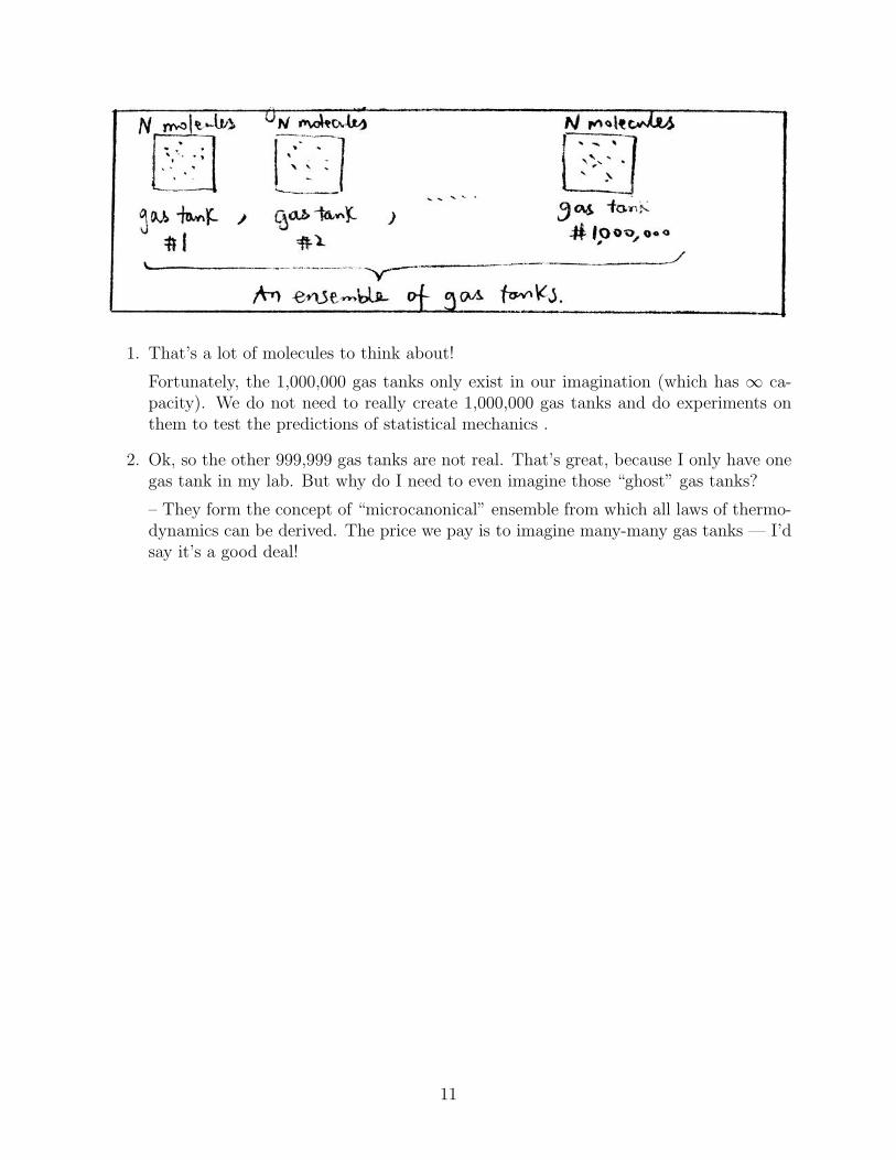
1. That’s a lot of molecules to think about!

Fortunately, the 1,000,000 gas tanks only exist in our imagination (which has ∞ ca-pacity). We do not need to really create 1,000,000 gas tanks and do experiments onthem to test the predictions of statistical mechanics .

2. Ok, so the other 999,999 gas tanks are not real. That’s great, because I only have onegas tank in my lab. But why do I need to even imagine those “ghost” gas tanks?

– They form the concept of “microcanonical” ensemble from which all laws of thermo-dynamics can be derived. The price we pay is to imagine many-many gas tanks — I’dsay it’s a good deal!

11

From Random Walk From Classical Mechanicsto Diffusion Equation to Thermodynamics

Step 1

one particle jump on a lattice one point move in 6N -dimensional(random) phase space (deterministic)

Step 2

many independent particles many copies of the system(random walkers) (gas tanks) corresponding to

on a lattice many points in the 6N -dimensionalphase space

– an ensemble of random walkers – an ensemble of gas tanks– so many that a density function – so many that a density function

C(x) makes sense ρ({qi}, {pi}) in Γ make sense

Step 3X(t) = X(0) +

∑i li µ = ω ∂H

∂µ

going to the continuum limit → going to the continuum limit →

Diffusion equation Liouville’s theorem

∂C(x,t)∂t

= D ∂2C(x,t)∂x2

dρdt≡ D ∂ρ

∂t+∑

i∂ρ∂qiqi +

∑i∂ρ∂pipi = 0

PDE for C(x, t) PDE for ρ({qi}, {pi}, t)(incompressible flow in Γ)

12

3 Liouville’s theorem

Liouville’s theorem states that the phase space density ρ(µ, t) behaves like anincompressible fluid.

So, after going to the continuum limit, instead of the diffusion equation, we get an equationin fluid mechanics.

How can we prove it?

3.1 Flow of incompressible fluid in 3D

Let’s first familiarize ourselves with the equations in fluid mechanics. Imagine a fluid con-sisting of a large number of particles with density ρ(x, t) ≡ ρ(x, y, z, t). Imagine that theparticles follow a deterministic (no diffusion) flow field v(x), i.e. vx(x, y, z), vy(x, y, z),vz(x, y, z) (velocity of the particle only depends on their current location). This tells us howto follow the trajectory of one particle.

How do we obtain the equation for ρ(x, t) from the flow field v(x)?

1. mass conservation (equation of continuity)

∂ρ(x, t)

∂t= −∇ · J = −

(∂

∂xJx +

∂

∂yJy +

∂

∂zJz

). (45)

2. flux for deterministic flow J(x) = ρ(x) v(x)

∂ρ(x, t)

∂t= −∇ · (ρ(x) v(x))

= −[∂

∂x(ρvx) +

∂

∂y(ρvy) +

∂

∂z(ρvz)

]= −

[(∂

∂xρ

)vx +

(∂

∂yρ

)vy +

(∂

∂zρ

)vz

]+[

ρ

(∂

∂xvx

)+ ρ

(∂

∂yvy

)+ ρ

(∂

∂zvz

)](46)

∂ρ

∂t= −(∇ρ) · v − ρ (∇ · v) (47)

13

∂ρ(x, y, z, t)/∂t describes the change of ρ with it at a fixed point (x, y, z).

We may also ask about how much the density changes as we move together with a particle,i.e., or how crowded a moving particle “feels” about its neighborhood. This is measured bythe total derivative,

dρ

dt=

∂ρ

∂t+ (∇ρ) · v =

∂ρ

∂t+∂ρ

∂xvx +

∂ρ

∂yvy +

∂ρ

∂zvz (48)

Hence the density evolution equation can also be expressed as

dρ

dt= −ρ (∇ · v) (49)

For incompressible flow,dρ

dt= 0 , ∇ · v = 0 (50)

a particle always feels the same level of “crowdedness”.

3.2 Flow in phase space

Why do we say the collective trajectories of an ensemble of points following Hamiltoniandynamics can be described by incompressible flow in phase space?

14

All points considered together follows incompressible flow. A point always find the samenumbers of neighbors per unit volume as it moves ahead with time.

real flow in 3D flow in 6N -D phase space

x, y, z q1, q2, · · · , q3N , p1, p2, · · · , p3N

∇ =(∂∂x, ∂∂y, ∂∂z

)∇ =

(∂∂q1, ∂∂q2, · · · , ∂

∂q3N, ∂∂p1, ∂∂p2, · · · , ∂

∂p3N

)v = (x, y, z) v = (q1, q2, · · · , q3N , p1, p2, · · · , p3N)

∂ρ∂t

= −∇(ρv) ∂ρ∂t

= −[∑3N

i=1∂∂qi

(ρqi) + ∂∂pi

(ρpi)]

= −(∇ρ)v − ρ(∇ · v) = −[∑3N

i=1∂ρ∂qiqi + ∂ρ

∂pipi

]−[∑3N

i=1 ρ∂qi∂qi

+ ρ∂pi∂pi

]dρdt≡= ∂ρ

∂t+ (∇ρ) · v = −ρ(∇ · v) dρ

dt≡ ∂ρ

∂t+∑3N

i=1∂ρ∂qiqi + ∂ρ

∂pipi = −ρ

[∑3Ni=1

∂qi∂qi

+ ∂pi∂pi

]flow is incompressible if flow is incompressible if

∇ · v = 0∑

i∂qi∂qi

+ ∂pi∂pi

= 0 (is this true?)

15

Proof of Liouville’s theorem (dρ/dt = 0)

Start from Hamilton’s equation of motion

qi =∂H

∂pi→ ∂qi

∂qi=

∂2H

∂pi∂qi(51)

pi = −∂H∂qi

→ ∂pi∂pi

= − ∂2H

∂pi∂qi(52)

∂qi∂qi

+∂pi∂pi

=∂2H

∂pi∂qi− ∂2H

∂pi∂qi= 0 (53)

Therefore, we obtaindρ

dt=∂ρ

∂t+∑i

∂ρ

∂qiqi +

∂ρ

∂pipi = 0 (54)

which is Liouville’s theorem.

Using Liouville’s theorem, the equation of evolution for the density function ρ({qi}, {pi}, t)can be written as

∂ρ

∂t= −

∑i

(∂ρ

∂qiqi +

∂ρ

∂pipi

)= −

∑i

(∂ρ

∂qi

∂H

∂pi− ∂ρ

∂pi

∂H

∂qi

)(55)

This can be written concisely using Poisson’s bracket,

∂ρ

∂t= −{ρ,H} (56)

Poisson’s bracket

{A,B} ≡3N∑i=1

(∂A

∂qi

∂B

∂pi− ∂A

∂pi

∂B

∂qi

)(57)

Obviously, {A,B} = −{B,A} and {A,A} = 0.

Not so obviously, {A,A2} = 0, and {A,B} = 0 if B is a function of A, i.e. B = f(A).

16

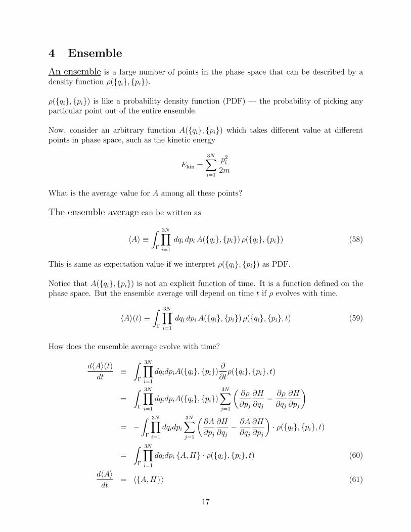
4 Ensemble

An ensemble is a large number of points in the phase space that can be described by adensity function ρ({qi}, {pi}).

ρ({qi}, {pi}) is like a probability density function (PDF) — the probability of picking anyparticular point out of the entire ensemble.

Now, consider an arbitrary function A({qi}, {pi}) which takes different value at differentpoints in phase space, such as the kinetic energy

Ekin =3N∑i=1

p2i

2m

What is the average value for A among all these points?

The ensemble average can be written as

〈A〉 ≡∫

Γ

3N∏i=1

dqi dpiA({qi}, {pi}) ρ({qi}, {pi}) (58)

This is same as expectation value if we interpret ρ({qi}, {pi}) as PDF.

Notice that A({qi}, {pi}) is not an explicit function of time. It is a function defined on thephase space. But the ensemble average will depend on time t if ρ evolves with time.

〈A〉(t) ≡∫

Γ

3N∏i=1

dqi dpiA({qi}, {pi}) ρ({qi}, {pi}, t) (59)

How does the ensemble average evolve with time?

d〈A〉(t)dt

≡∫

Γ

3N∏i=1

dqidpiA({qi}, {pi})∂

∂tρ({qi}, {pi}, t)

=

∫Γ

3N∏i=1

dqidpiA({qi}, {pi})3N∑j=1

(∂ρ

∂pj

∂H

∂qj− ∂ρ

∂qj

∂H

∂pj

)

= −∫

Γ

3N∏i=1

dqidpi

3N∑j=1

(∂A

∂pj

∂H

∂qj− ∂A

∂qj

∂H

∂pj

)· ρ({qi}, {pi}, t)

=

∫Γ

3N∏i=1

dqidpi {A,H} · ρ({qi}, {pi}, t) (60)

d〈A〉dt

= 〈{A,H}〉 (61)

17

(Very similar equation appears in quantum mechanics!)

For example, average total energy among all points in the ensemble

Etot ≡ 〈H〉 (62)

dEtotdt

=d〈H〉dt

= 〈{H,H}〉 = 0 (63)

This is an obvious result, because the total energy of each point is conserved as they movethrough the phase space. As a result, the average total energy also stays constant.

Example 5. Pendulum with Hamiltonian

H(θ, pθ) =p2θ

2mR2+mgR cos θ

Phase space is only 2-dimensional (θ, pθ).

Equilibrium motion of one point in phase space is

θ =∂H

∂pθpθ = −∂H

∂θ(64)

Now consider a large number of points in the (θ, pθ) space. p(θ, pθ, t) describes their densitydistribution at time t.

What is the evolution equation for ρ?

∂p(θ, pθ, t)

∂t= −∂ρ

∂θθ − ∂ρ

∂pθpθ

= −∂ρ∂θ

∂H

∂pθ+∂ρ

∂pθ

∂H

∂θ≡ −{ρ,H} (65)

18

From ∂H∂pθ

= pθmR2 , ∂H

∂θ= −mgR sin θ

⇒ ∂ρ

∂t= −∂ρ

∂θ

pθmR2

− ∂ρ

∂pθmgR sin θ (66)

Suppose A = θ2, the ensemble average of A is

〈A〉 =

∫dθdpθ θ

2 ρ(θ, pθ, t) (67)

How does 〈A〉 changes with time?

d〈A〉dt

= 〈{A,H}〉 (68)

{A,H} =∂θ2

∂θ

∂H

∂pθ− ∂θ2

∂pθ

∂H

∂θ= 2θ(−mgR sin θ) (69)

⇒ d〈A〉dt

=d〈θ2〉dt

= −2mgR 〈θ sin θ〉 (70)

Example 6. Consider an ensemble of pendulums described in Example 5. At t = 0, thedensity distribution in the ensemble is,

ρ(θ, pθ, t = 0) =1

2π

1√2πσ

exp

[− p2

θ

2σ2

](71)

where −π ≤ θ < π, −∞ < pθ <∞.

(a) Verify that ρ(θ, pθ, t = 0) is properly normalized.

(b) What is ∂ρ/∂t|t=0? Mark regions in phase space where ∂ρ/∂t|t=0 > 0 and regions where∂ρ/∂t|t=0 < 0.

(c) How can we change ρ(θ, pθ, t = 0) to make ∂ρ/∂t = 0?

19

5 Summary

By the end of this lecture, you should:

• be able to derive the equations of motion of a mechanical system by constructing a La-grangian, and obtain the Hamitonian through Legendre transform. (This is importantfor Molecular Simulations.)

• agree with me that the flow of an ensemble of points in phase space, each following theHamilton’s equation of motion, is the flow of an incompressible fluid.

• be able to write down the relation between partial derivative and total derivative ofρ({qi}, {pi}, t).

• be able to write down the equation of Liovielle’s theorem (close book, of course).

• be able to express the ensemble average of any quantity as an integral over phase space,and to write down the time evolution of the ensemble average (be ware of the minussign!)

The material in this lecture forms (part of) the foundation of statistical mechanics.

As an introductory course, we will spend more time on how to use statistical mechanics.

A full appreciation of the foundation itself will only come gradually with experience.

Nonetheless, I think an exposure to the theoretical foundation from the very beginning is agood idea.

References

1. Landau and Lifshitz, Mechanics, 3rd. ed., Elsevier, 1976. Chapter I, II, VII.

20