This content has been downloaded from IOPscience. Please scroll down to see the full text.

Download details:

IP Address: 131.188.201.35

This content was downloaded on 23/07/2014 at 07:14

Please note that terms and conditions apply.

Classical entanglement in polarization metrology

View the table of contents for this issue, or go to the journal homepage for more

2014 New J. Phys. 16 073019

(http://iopscience.iop.org/1367-2630/16/7/073019)

Home Search Collections Journals About Contact us My IOPscience

Classical entanglement in polarization metrology

Falk Töppel1,2,3, Andrea Aiello1,2, Christoph Marquardt1,2,Elisabeth Giacobino1,4 and Gerd Leuchs1,21Max Planck Institute for the Science of Light, Günther-Scharowsky-Straße 1/Bldg. 24,D-91058 Erlangen, Germany2 Institute for Optics, Information and Photonics, Universität Erlangen-Nürnberg, Staudtstraße7/B2, D-91058 Erlangen, Germany3 Erlangen Graduate School in Advanced Optical Technologies (SAOT), Paul-Gordan-Straße 6,D-91052 Erlangen, Germany4 Laboratoire Kastler Brossel, Université Pierre et Marie Curie, Ecole Normale Supérieure,CNRS, 4 place Jussieu, F-75252 Paris Cedex 05, FranceE-mail: falk.toeppel@mpl.mpg.de

Received 3 April 2014, revised 22 May 2014Accepted for publication 13 June 2014Published 16 July 2014

New Journal of Physics 16 (2014) 073019

doi:10.1088/1367-2630/16/7/073019

AbstractQuantum approaches relying on entangled photons have been recently proposedto increase the efficiency of optical measurements. We demonstrate here that,surprisingly, the use of classical light with entangled degrees of freedom can alsobring outstanding advantages over conventional measurements in polarizationmetrology. Specifically, we show that radially polarized beams of light allow toperform real-time single-shot Mueller matrix polarimetry. Our results alsoindicate that quantum optical procedures requiring entanglement without non-locality can be actually achieved in the classical optics regime.

Keywords: entanglement and quantum nonlocality, applied classical electro-magnetism, polarization

1. Introduction

In the last years, quantum information theory taught us that the use of entangled photons offersthe unique advantage over classical light of providing more information in metrologyapplications, imaging and, more generally, in optical measurements [1–6]. However,

Content from this work may be used under the terms of the Creative Commons Attribution 3.0 licence.Any further distribution of this work must maintain attribution to the author(s) and the title of the work, journal

citation and DOI.

New Journal of Physics 16 (2014) 0730191367-2630/14/073019+21$33.00 © 2014 IOP Publishing Ltd and Deutsche Physikalische Gesellschaft

entanglement is not necessarily a signature of the quantum mechanical nature of a system.Indeed, one can distinguish between two types of entanglement: a) entanglement betweenspatially separated systems (inter-system entanglement) and b) entanglement between differentdegrees of freedom (DoFs) of a single system (intra-system entanglement) [7, 8]. Inter-systementanglement, or ‘nonlocal entanglement’, can occur only in bona fide quantum systems andmay yield to nonlocal statistical correlations. Conversely, intra-system entanglement, or ‘localentanglement’, may also appear in classical systems and cannot generate nonlocal correlations[9]. As an example, photon pairs from atomic cascades [10] show nonlocal entanglement. Incontrast, local entanglement can be found, e.g., between spatial and spin DoFs in singleneutrons [11]. In classical optics, local entanglement between polarization and spatial DoFs ofthe same beam has been lately demonstrated in radially and azimuthally polarized beams oflight [12–18]. Hereafter, we shall denote the occurrence of local entanglement in classicalsystems by ‘classical entanglement’ [8]5.

Recently, is has been suggested that quantum computing tasks requiring entanglement butnot nonlocality can be efficiently accomplished in the classical optical regime [15, 22, 23].However, when and how classical entanglement can be exploited in lieu of nonlocalentanglement to improve techniques of optical metrology, still remain largely open questions[24, 25].

In this work, we address some of these central issues by illustrating a representativeexample of the peculiar entanglement between polarization and spatial modes in radiallypolarized beams of light and its possible use for enhancing the efficiency of Mueller matrixpolarimetry. The underlying idea is simple: in a conventional Mueller matrix measurementsetting [26–29], an either transmissive or scattering material sample (the object) is illuminatedwith a light beam (the probe) prepared in, at least, four different polarization states in a temporalsequence. From the analysis of the polarization of the light transmitted or scattered, the opticalproperties of the object can be inferred. In the alternative setting we propose here, the object isprobed only once with one light beam of radial polarization, as opposed to four differentlypolarized beams. Then, the light transmitted or reflected by the object is analyzed both inpolarization and in spatial DoFs by means of suitable polarization and spatial mode selectors. Inour setting, the polarization DoFs of the beam are used to actually probe the object and thespatial DoFs are used to post-select the polarization state of the light: this is the main ideapresented in this work. This scheme, in principle, outperforms conventional ones because theradially polarized beam carries all polarizations at once in a classically entangled state, thusproviding for a sort of ‘polarization parallelism’. For all practical applications where the opticalproperties of the sample change rapidly with time, our method presents an advantage overconventional Mueller matrix polarimetry [26, 27, 30–35]. However, in practice, the detectionsetup required by our scheme is more involved than a conventional polarimetry one and is,therefore, potentially more sensitive to measurement errors.

Although our conclusions here are strictly valid only for optical elements that do not altersignificantly the spatial structure of the probe beam, this is not a serious restriction. Forexample, all optical elements routinely used on an optical bench like single-mode fibers,retardation plates, birefringent prisms, optical rotators, etc, fall in this category. Anotherrequirement for the validity of our scheme is that the polarization properties of the sample must

5 In the literature this phenomenon is also refereed to as ‘structural inseparability’ [19, 20] and ‘nonquantumentanglement’ [21].

2

New J. Phys. 16 (2014) 073019 F Töppel et al

be homogeneous over the beam cross section. Considering that an ordinary radially polarizedbeam of light may be prepared with a waist of the order of hundreds of μm, such a requirementdoes not represent an actual limitation.

2. Jones vectors, entanglement and radially polarized beams

Consider a monochromatic beam of light of angular frequency ω, propagating along the z-axis of aCartesian reference frame x y z( , , ) and polarized in the (x, y) plane. In the paraxial approximation[36], the electric field can be written as ω= −E r E rt kz t( , ) Re [ ( ) exp (i( ))], where6

ψ= +( )E r e e rA A( ) ( ), (1)x y0 1

with ψ r( ) denoting the spatial mode of the beam, e e,x y and ez being unit vectors in the x, y and zdirections, respectively. In the expression above, = + +r e e ex y zx y z stands for the positionvector, and the two complex numbers A0 and A1 represent the amplitudes of the electric field alongthe x- and y-axis, respectively. A convenient vector notation for fields of the form (1) wasintroduced by R C Jones in the 1940s [27, 37]:

ψ=⎡⎣⎢

⎤⎦⎥E r r

A

A( ) ( ). (2)

0

1

With this notation, the identification of the polarization and the spatial DoFs, represented by theJones vector A A[ , ]T

0 1 and the scalar field ψ r( ), respectively, becomes straightforward.For a field of the form (2), polarization and spatial DoFs are said to be separable [13]

because the expression of E r( ) is factorizable in the product of a single space independentvector, and a single scalar field. This mathematical property reflects the absence of physicalcoupling between polarization and spatial DoFs. However, in general, polarization and spatialDoFs can be coupled and when this happens the factorizable representation (2) is no longervalid. Consider, for example, the electric field of a beam of light nonuniformly polarized in the(x, y) plane, which can be expressed as

ψ ψ ψ ψ= + + +E r e r e r e r e rA A A A( ) ( ) ( ) ( ) ( ), (3)x x y y00 10 01 01 10 10 11 01

where ψ r( )mn , with ∈ …m n, {0, 1, 2, }, is the Hermite–Gauss (HG) solution of the paraxialwave equation of order = +N m n [36] and Aij denotes a complex amplitude of the field, with

∈i j, {0, 1}. In the Jones notation, (3) takes either of the two following forms:

ψ ψψ ψ

=++

⎡⎣⎢

⎤⎦⎥E r

r r

r r

A A

A Aa( )

( ) ( )

( ) ( )(4 )

00 10 01 01

10 10 11 01

ψ ψ= +⎡⎣⎢

⎤⎦⎥

⎡⎣⎢

⎤⎦⎥r r

A

A

A

Ab( ) ( ). (4 )

00

1010

01

1101

By writing the electric field as in (4a), it follows that the beam has a nonuniformpolarization pattern because the Jones vector varies with the position vector r. On the otherhand, when E r( ) is written in the form (4b), it appears evident that polarization and spatial

6 Please note that here ψ ψ=r x y z( ) ( , ; ) is a paraxial field, so x y, are the Cartesian coordinates in the transverseplane and z must be considered as a varying parameter.

3

New J. Phys. 16 (2014) 073019 F Töppel et al

DoFs are now nonseparable, or entangled, because one needs two coordinate-independentJones vectors and two independent scalar fields, ψ10 and ψ01,

7 to represent the electric field.Mathematically speaking, occurrence of entanglement requires an expression to be written

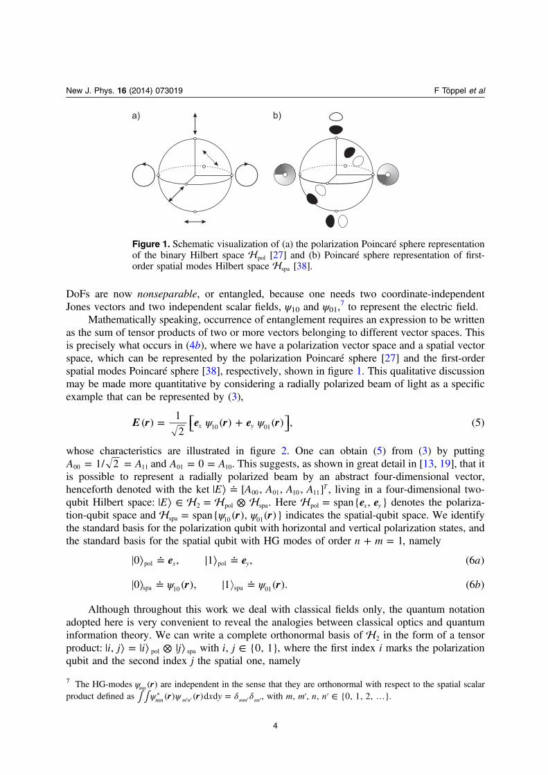
as the sum of tensor products of two or more vectors belonging to different vector spaces. Thisis precisely what occurs in (4b), where we have a polarization vector space and a spatial vectorspace, which can be represented by the polarization Poincaré sphere [27] and the first-orderspatial modes Poincaré sphere [38], respectively, shown in figure 1. This qualitative discussionmay be made more quantitative by considering a radially polarized beam of light as a specificexample that can be represented by (3),

ψ ψ= +⎡⎣ ⎤⎦E r e r e r( )1

2( ) ( ) , (5)x y10 01

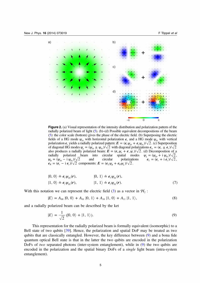
whose characteristics are illustrated in figure 2. One can obtain (5) from (3) by putting= =A A1/ 200 11 and = =A A001 10. This suggests, as shown in great detail in [13, 19], that it

is possible to represent a radially polarized beam by an abstract four-dimensional vector,henceforth denoted with the ket | ⟩ ≐E A A A A[ , , , ]T

00 01 10 11 , living in a four-dimensional two-qubit Hilbert space: | ⟩ ∈ = ⊗ E 2 pol spa. Here = e espan{ , }x ypol denotes the polariza-tion-qubit space and ψ ψ= r rspan{ ( ), ( )}spa 10 01 indicates the spatial-qubit space. We identifythe standard basis for the polarization qubit with horizontal and vertical polarization states, andthe standard basis for the spatial qubit with HG modes of order + =n m 1, namely

∣ ⟩ ≐ ∣ ⟩ ≐e e a0 , 1 , (6 )x ypol pol

ψ ψ∣ ⟩ ≐ ≐r r b0 ( ), 1 ( ). (6 )spa 10 spa 01

Although throughout this work we deal with classical fields only, the quantum notationadopted here is very convenient to reveal the analogies between classical optics and quantuminformation theory. We can write a complete orthonormal basis of 2 in the form of a tensorproduct: | ⟩ = | ⟩ ⊗ | ⟩i j i j, pol spa with ∈i j, {0, 1}, where the first index i marks the polarizationqubit and the second index j the spatial one, namely

Figure 1. Schematic visualization of (a) the polarization Poincaré sphere representationof the binary Hilbert space pol [27] and (b) Poincaré sphere representation of first-order spatial modes Hilbert space spa [38].

7 The HG-modes ψ r( )mn are independent in the sense that they are orthonormal with respect to the spatial scalarproduct defined as ∫ ∫ ψ ψ δ δ=′ ′ ′ ′

* r r x y( ) ( )d dmn m n mm nn , with ′ ′ ∈ …m m n n, , , {0, 1, 2, }.

4

New J. Phys. 16 (2014) 073019 F Töppel et al

ψ ψψ ψ

≐ ≐≐ ≐

e r e r

e r e r

0, 0 ( ), 0, 1 ( ),

1, 0 ( ), 1, 1 ( ). (7)x x

y y

10 01

10 01

With this notation we can represent the electric field (3) as a vector in 2 :

= + + +E A A A A0, 0 0, 1 1, 0 1, 1 , (8)00 01 10 11

and a radially polarized beam can be described by the ket

= +E1

2( 0, 0 1, 1 ). (9)

This representation for the radially polarized beam is formally equivalent (isomorphic) to aBell state of two qubits [39]. Hence, the polarization and spatial DoF may be treated as twoqubits that are classically entangled. However, the key difference between (9) and a bona fidequantum optical Bell state is that in the latter the two qubits are encoded in the polarizationDoFs of two separated photons (inter-system entanglement), while in (9) the two qubits areencoded in the polarization and the spatial binary DoFs of a single light beam (intra-systementanglement).

Figure 2. (a) Visual representation of the intensity distribution and polarization pattern of theradially polarized beam of light (5). (b)–(d) Possible equivalent decompositions of the beam(5): the color scale (bottom) gives the phase of the electric field. (b) Superposing the electricfields of a HG mode ψ10 with horizontal polarization ex and a HG mode ψ01 with verticalpolarization ey yields a radially polarized pattern: ψ ψ= +E e e( )/ 2x y10 01 . (c) Superpositionof diagonal HG modes ψ ψ ψ= ±± ( )/ 210 01 with diagonal polarizations = ±±e e e( )/ 2x y

also produces a radially polarized beam: ψ ψ= ++ + − −E e e( )/ 2 . (d) Decomposition of aradially polarized beam into circular spatial modes ψ ψ ψ= +( i )/ 2L 10 01 ,ψ ψ ψ= −( i )/ 2R 10 01 and circular polarizations = +e e e( i )/ 2L x y ,

= −e e e( i )/ 2R x y components: ψ ψ= +E e e( )/ 2L R R L .

5

New J. Phys. 16 (2014) 073019 F Töppel et al

3. Stokes parameters and the Liouville representation of a quantum state

The representations (3) and (8) for the electric field of a light beam are adequate as long as oneis concerned with detection schemes that can resolve both polarization and spatial DoFs. Whenthis is not the case, as in conventional Mueller matrix polarimetry, it becomes necessary tointroduce a more general representation, namely the 4 × 4 coherency matrix ρ of the field,defined in terms of the electric field amplitudes Aij as

ρ= =

* * * *

* * * *

* * * *

* * * *

⎡

⎣

⎢⎢⎢⎢⎢

⎤

⎦

⎥⎥⎥⎥⎥

E E

A A A A A A A A

A A A A A A A A

A A A A A A A A

A A A A A A A A

. (10)

00 00 00 01 00 10 00 11

01 00 01 01 01 10 01 11

10 00 10 01 10 10 10 11

11 00 11 01 11 10 11 11

Of course, at this stage (10) still contains the same amount of information as (8). As a specificexample, the coherency matrix of the radially polarized beam (9) can be simply written as

ρ =

⎡

⎣

⎢⎢⎢

⎤

⎦

⎥⎥⎥

12

1 0 0 10 0 0 00 0 0 01 0 0 1

. (11)

Suppose now to have a detection scheme that is not capable of resolving the spatial DoFs.In this case, (8) would furnish redundant information about the spatial DoFs that is not at ourdisposal. However, a proper representation of the beam can then be obtained from (10) bytracing out the unobservable spatial DoFs. In this manner one obtains the reduced 2 × 2polarization coherency matrix ρpol that encodes all the available information about thepolarization of the light beam, irrespective of the spatial DoFs:

∑

ρ ρ ρ

ρ

→ =

=

==

†

i i

AA

tr ( )

, (12)i

pol spa

0

1

spa spa

where …tr ( )spa denotes the trace with respect to the spatial DoFs and the spatial kets | ⟩0 spa and| ⟩1 spa are defined in (6b). Here

=⎡⎣⎢

⎤⎦⎥A

A A

A A, (13)

00 01

10 11

is a 2 × 2 matrix whose elements are the coefficients Aij of the ket expansion (8). In a similarmanner, one can calculate the reduced 2 × 2 spatial coherency matrix ρspa that encodes all theavailable information about the spatial modes of the light beam, irrespective of the polarization:

ρ ρ=

= †( )A A

tr ( )

, (14)T

spa pol

where …tr ( )pol denotes the trace with respect to the polarization DoFs.

6

New J. Phys. 16 (2014) 073019 F Töppel et al

From the definition (12) it follows that ρpol is Hermitian and positive semidefinite.Therefore, it admits a Liouville representation of the form

∑ρ σ=μ

μ μ=

S12

, (15)pol0

3

where the coefficients μS are real numbers and the set σμ μ ={ } 03 of 2 × 2 Hermitean matrices forms

a complete basis of observables [40]. The factor 1/2 in front of (15) is conventional. In classicalpolarization optics, the coefficients μS are known as the Stokes parameters of the beam [41] andthe basis set σ μ =μ{ } 0

3 is constituted by the four Pauli matrices

σ σ

σ σ

= =

= − = −

⎡⎣⎢

⎤⎦⎥

⎡⎣⎢

⎤⎦⎥

⎡⎣⎢

⎤⎦⎥

⎡⎣⎢

⎤⎦⎥

1 00 1

, 0 11 0

,

0 ii 0

, 1 00 1

, (16)

0 1

2 3

which are orthogonal with respect to the scalar product defined as σ σ δ=μ ν μνtr ( ) 2 . From thisproperty and the definition (15) it follows that

ρ σ=μ μ( )S tr . (17)pol

For the radially polarized beam (9), = A / 22 and ρ ρ= = /2pol 2 spa, where 2 denotesthe 2 × 2 identity matrix. In the language of classical polarization optics, this means that theradially polarized beam is completely unpolarized: = =S S S S S[ , , , ] [1, 0, 0, 0]T T

0 1 2 3 . Thisobservation may appear confusing because (4a) and figure 2 show that a radially polarizedbeam possesses a well defined local, i.e. defined at each point (x, y) of its transverse spatialprofile, Jones vector given by

ψψ

=⎡⎣⎢

⎤⎦⎥E r

r

r( )

1

2

( )

( ). (18)

10

01

However, ρpol is obtained from ρ after tracing out the spatial DoFs. From a physical point ofview, this corresponds to measuring the global Stokes parameters of the beam, as a whole, with‘bucket’ detectors that integrate the intensity of light over all the cross section of the beam. Asimilar situation is encountered for photon-pairs in a Bell state: Although the polarization of thetwo-photon state is perfectly defined (pure state), each of the two photons, when observedseparately, appears as completely unpolarized (mixed state) [42].

4. Mueller matrix polarimetry

Typically, in a conventional polarimetry setup, an either transmissive or scattering materialsample (the object) is illuminated with a light beam (input beam) that, as a result of theinteraction with the object, emerges transformed (output beam). In this section we will studyhow radially polarized beams transform under the action of a polarization-affecting opticalelement, having in mind the final goal of measuring the Mueller matrix of the latter. From amathematical point of view, here we consider local linear transformations of the form

⊗T Tpol spa, namely transformations that act on each DoF separately, where → T :d d d with∈d {pol, spa} is a 2 × 2 complex matrix known as Jones matrix in polarization optics. As in

7

New J. Phys. 16 (2014) 073019 F Töppel et al

this work we are concerned with optical elements affecting polarization DoFs solely, henceforthwe assume = Tspa 2, and we will omit the subscript ‘pol’ in Tpol.

Under the action of T, the generic ket (8) transforms as

∑

→ ′ = ⊗

= ′=

( )E E T E

A i j, , (19)i j

2

, 0

1

ij

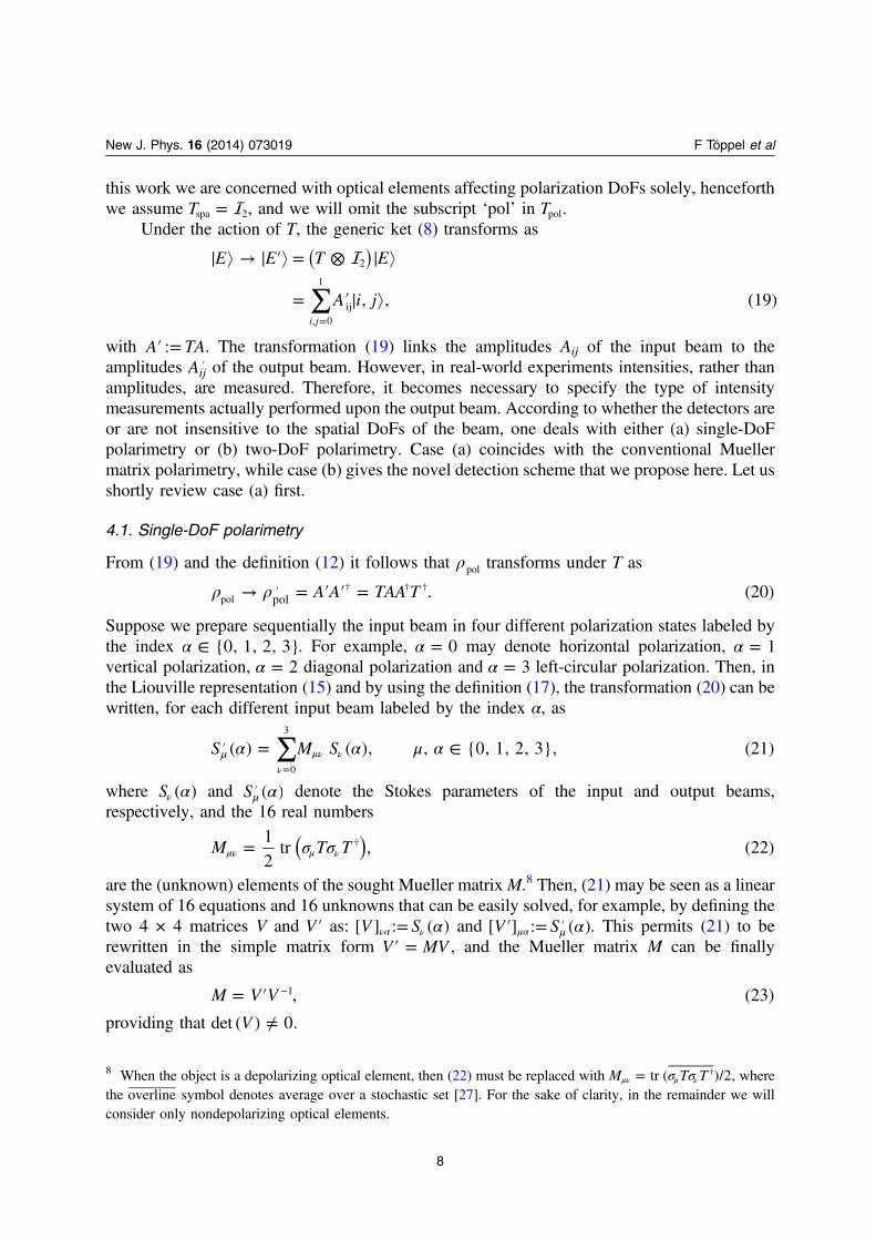
with ′ =A TA: . The transformation (19) links the amplitudes Aij of the input beam to theamplitudes ′Aij of the output beam. However, in real-world experiments intensities, rather thanamplitudes, are measured. Therefore, it becomes necessary to specify the type of intensitymeasurements actually performed upon the output beam. According to whether the detectors areor are not insensitive to the spatial DoFs of the beam, one deals with either (a) single-DoFpolarimetry or (b) two-DoF polarimetry. Case (a) coincides with the conventional Muellermatrix polarimetry, while case (b) gives the novel detection scheme that we propose here. Let usshortly review case (a) first.

4.1. Single-DoF polarimetry

From (19) and the definition (12) it follows that ρpol transforms under T as

ρ ρ→ = ′ ′ =′ † † †A A TAA T . (20)polpol

Suppose we prepare sequentially the input beam in four different polarization states labeled bythe index α ∈ {0, 1, 2, 3}. For example, α = 0 may denote horizontal polarization, α = 1vertical polarization, α = 2 diagonal polarization and α = 3 left-circular polarization. Then, inthe Liouville representation (15) and by using the definition (17), the transformation (20) can bewritten, for each different input beam labeled by the index α, as

∑α α μ α= ∈μ′

νμν ν

=

S M S( ) ( ), , {0, 1, 2, 3}, (21)0

3

where ανS ( ) and αμ′S ( ) denote the Stokes parameters of the input and output beams,respectively, and the 16 real numbers

σ σ=μν μ ν†( )M T T

12

tr , (22)

are the (unknown) elements of the sought Mueller matrixM.8 Then, (21) may be seen as a linearsystem of 16 equations and 16 unknowns that can be easily solved, for example, by defining thetwo 4 × 4 matrices V and ′V as: α=να νV S[ ] : ( ) and α′ = μ′μαV S[ ] : ( ). This permits (21) to berewritten in the simple matrix form ′ =V MV , and the Mueller matrix M can be finallyevaluated as

= ′ −M V V , (23)1

providing that ≠Vdet ( ) 0.

8 When the object is a depolarizing optical element, then (22) must be replaced with σ σ=μν μ ν†M T Ttr ( )/2, where

the overline symbol denotes average over a stochastic set [27]. For the sake of clarity, in the remainder we willconsider only nondepolarizing optical elements.

8

New J. Phys. 16 (2014) 073019 F Töppel et al

This is the essence of conventional Mueller matrix polarimetry [43]. Of course, in a situationwhere experimental errors may occur, the simple linear inversion algorithm (23) often does notsuffice and more sophisticated inversion methods must be used instead [28, 29]. However, thelesson to be learned here is that conventional Mueller matrix polarimetry needs the input beam tobe sequentially prepared in, at least, four different polarization states to gain complete informationabout the object. Conversely, we are going to show soon how the same amount of information canbe obtained by probing the object only once with a radially polarized beam.

4.2. Two-DoF polarimetry

We now consider a detection scheme that is capable of resolving both the polarization and the spatialDoFs. The complete coherency matrix (10) can also be written in a Liouville form similar to (15) as

∑ρ σ σ= ⊗μ ν

μν μ ν=

( )S14

, (24), 0

3

where we have defined the two-DoFs Stokes parameters as9

ρ σ σ= ⊗μν μ ν⎡⎣ ⎤⎦( )S tr . (25)

These quantities are the classical optics analogue of the two-photon Stokes parametersintroduced in [44, 45]. However, while in [45] the two polarization qubits are encoded in twoseparated photons, in our case the polarization qubit and the spatial qubit are encoded in thesame radially polarized beam of light. Therefore, the two-DoFs Stokes parameters give theintrabeam correlations between polarization and spatial DoFs [46]. In order to measure thesecorrelations, one needs a detection scheme capable of resolving both DoFs. Such anexperimental apparatus will be studied in the next section. For the radially polarized beamrepresented by (11), the two-DoFs Stokes parameters take the particularly simple form

λ δ λ= = −μ =μν μ μν μ { }{ }S , where 1, 1, 1, 1 . (26)

0

3

From (19) it follows that, under the action of T, (11) transforms as

∑

ρ ρ ρ

λ σ σ

→ = ⊗ ⊗

= ⊗

′

μμ μ μ

†

=

†

( )

( )

( )T T

T T14

. (27)

2 2

0

3

Substituting (27) into (25) yields

∑

ρ σ σ

λ σ σ σ σ

λ

′ = ′ ⊗

=

=

μν μ ν

αα μ α α ν

μν ν

=

†

⎡⎣ ⎤⎦( )

( )

S

T T

M

tr

14

tr tr ( )

, (28)0

3

9 Here we are using the standard properties of the direct product of matrices: ⊗ ⊗ = ⊗A B C D AC BD( ) ( ) and⊗ =A B A Btr ( ) tr ( ) tr ( ).

9

New J. Phys. 16 (2014) 073019 F Töppel et al

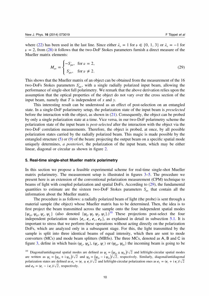
where (22) has been used in the last line. Since either λ =ν 1 for ν ∈ {0, 1, 3} or λ = −ν 1 forν = 2, from (28) it follows that the two-DoF Stokes parameters furnish a direct measure of theMueller matrix elements:

ν

ν=

− =

≠μν

μν

′

′μν ⎪

⎪⎧⎨⎩

MS

S

, for 2,

, for 2.(29)

This shows that the Mueller matrix of an object can be obtained from the measurement of the 16two-DoFs Stokes parameters μν′S , with a single radially polarized input beam, allowing theperformance of single-shot full polarimetry. We remark that the above derivation relies upon theassumption that the optical properties of the object do not vary over the cross section of theinput beam, namely that T is independent of x and y.

This interesting result can be understood as an effect of post-selection on an entangledstate. In a single-DoF polarimetry setup, the polarization state of the input beam is preselectedbefore the interaction with the object, as shown in (21). Consequently, the object can be probedby only a single polarization state at a time. Vice versa, in our two-DoF polarimetry scheme thepolarization state of the input beam is post-selected after the interaction with the object via thetwo-DoF correlation measurements. Therefore, the object is probed, at once, by all possiblepolarization states carried by the radially polarized beam. This magic is made possible by theentangled structure (5) or (9) of the beam: projecting the output beam on a specific spatial modeuniquely determines, a posteriori, the polarization of the input beam, which may be eitherlinear, diagonal or circular as shown in figure 2.

5. Real-time single-shot Mueller matrix polarimetry

In this section we propose a feasible experimental scheme for real-time single-shot Muellermatrix polarimetry. The measurement setup is illustrated in figures 3–5. The procedure wepresent here is an extension of the conventional polarization measurement (CPM) technique tobeams of light with coupled polarization and spatial DoFs. According to (29), the fundamentalquantities to estimate are the sixteen two-DoF Stokes parameters μνS that contain all theinformation about the Mueller matrix.

The procedure is as follows: a radially polarized beam of light (the probe) is sent through amaterial sample (the object) whose Mueller matrix has to be determined. Then, the idea is tofirst project the beam transmitted across the sample onto the four independent spatial modesψ ψ ψ ψ+{ , , , }L10 01 (also denoted ψ ψ ψ ψ{ , , , }0 1 2 3 .)10 These projections post-select the fourindependent polarization states +e e e e{ , , , }x y R , as explained in detail in subsection 5.1. It isimportant to stress that we perform these operations without acting directly on the polarizationDoFs, which are analyzed only in a subsequent stage. For this, the light transmitted by thesample is split into three identical beams of equal intensity, which then are sent to modeconverters (MCs) and mode beam splitters (MBSs). The three MCs, denoted as A, B and C infigure 3, define in which basis ψ ψ( , )L R , ψ ψ+ −( , ) or ψ ψ( , )10 01 the incoming beam is going to be

10 Diagonal/antidiagonal spatial modes are defined as ψ ψ ψ= ±± ( )/ 210 01 and left/right-circular spatial modesare written as ψ ψ ψ= +( )i / 2L 10 01 and ψ ψ ψ= −( )i / 2R 10 01 , respectively. Similarly, diagonal/antidiagonalpolarization states are defined as = ±±e e e( )/ 2x y and left/right-circular polarization ones as = +e e e( i )/ 2L x y

and = −e e e( i )/ 2R x y , respectively.

10

New J. Phys. 16 (2014) 073019 F Töppel et al

measured. MC A, which transforms the modes ψ ψ( , )L R into ψ ψ( , )10 01 , is made of aπ /2-converter, rotated by the angle θ π= /4 with respect to the horizontal axis (seeappendix A). MC B, which transforms the modes ψ ψ+ −( , ) into ψ ψ( , )10 01 , is made of a π-converter, rotated by the angle θ π= /8 with respect to the horizontal axis (see appendix A).MCC is made of empty space and does not change the modes. It can be shown [47] that a π-MCcan be physically realized with two identical cylindrical lenses separated by a distance f2 equalto two focal lengths ( f2 CL), as shown in figure 4 (a). Similarly, a π /2-MC is made from twoidentical cylindrical lenses separated by a distance f2 ( f2 CL), as illustrated in figure 4(b).Each MC is coupled to a MBS, which splits up a beam into its ψ10 and ψ01 spatial components.The MBS is made of a modified Mach–Zehnder interferometer (MZ) with an extra mirror in one

Figure 3. Schematic setup for real-time single-shot Mueller matrix polarimetry. Theradially polarized input beam ρ propagates through a material sample (object) whoseMueller matrix must be determined. The light ρ′ transmitted by the sample is split bypolarization maintaining beam splitters (BSs) into three identical beams and sentthrough mode converters (MCs) followed by mode beam splitters (MBSs). The ratios oftransmission (t) and reflection (r) coefficients of the BSs | | | |t r:2 2 are indicated in thefigure. Each combination of a MC with a MBS effectively projects the entering beamonto the specific spatial mode represented schematically in the figure. These operationspost-select the polarization of the input beam as explained in the text. The four outputports of the three MBSs projecting onto the spatial modes ψ ψ ψ ψ+{ , , , }L10 01 (alsodenoted ψ ψ ψ ψ{ , , , }0 1 2 3 ), are coupled to four distinct conventional polarizationmeasurement setups (CPMs). Each CPM delivers the intensities of the four polarizationcomponents +e e e e{ , , , }x y L (also denoted e e e e{ , , , }0 1 2 3 ), per each of the four enteringbeams ψ10, ψ01, ψ+ or ψL. The detectors labeled with the polarization-spatial indices αβwith α β ∈, {0, 1, 2, 3} in the figure, return the × =4 4 16 intensities αβI , where, forexample, ψ ρ ψ= ⟨ | ′| ⟩e eI , ,y y10 10 10 . From these intensities the two-DoF Stokes parameters

μνS and the Mueller matrix can be completely determined via (A.13) and (29). In a setupthat suffers from experimental imperfections, the intensities obtained by the 10additional detectors displayed in light gray may be needed. Physical implementations ofthe MCs, MBS and CPM are shown in figures 4 and 5.

11

New J. Phys. 16 (2014) 073019 F Töppel et al

arm and a half-wave plate (HWP) in the other arm, followed by another HWP in one outputport, as shown in figure 4 (d) (see appendix B and [48, 49]). As a result of these transformations,the MBS placed behind MC A splits up the incoming beam into its circular spatial components,ψL and ψR, MCB splits the beam into its diagonal and antidiagonal spatial components ψ+ and ψ-and MC C into the ψ10 and ψ01 components. By selecting one of the outputs of MBS A and ofMBS B and the two outputs of MBS C, one has access to the four spatial modesψ ψ ψ ψ+{ , , , }L10 01 . With this operation, we have physically acted only upon the spatial modes ofthe beam, and we will now analyze their polarization. This corresponds to a post-selection ofthe polarization state of the probe beam. This is possible thanks to the entanglement between thepolarization and the spatial DoFs.

The light exiting an output port of each MBS can be either directly detected, or sentthrough a CPM setup shown in figure 5. A beam entering the CPM is split into three beams ofequal intensity. Each beam passes through a polarization converter (PC) denoted A, B and C infigure 3. They are made from, respectively, a) a quarter-wave plate (QWP) whose fast axis istilted by π /4 with respect to the horizontal direction; b) a HWP with the fast axis rotated by π /8with respect to the horizontal direction; and c) empty space. Each PC is coupled to a polarizingbeam splitter (PBS), which splits a beam into its horizontal ex and vertical ey polarizationcomponents. The three combinations A, B and C of PCs and PBSs project the entering beamsonto three mutually unbiased pairs of polarization states, namely, a) horizontal/vertical:e e{ , }x y ; b) diagonal/antidiagonal: + −e e{ , }; and c) left/right-circular: e e{ , }L R , respectively.The intensity αβI of the light projected in the state ψα βe is recorded by a photo-detector that is

Figure 4. Physical implementation of mode converters (MCs) and the mode beamsplitter (MBS) used in figure 3. (a) MC A comprises a pair of identical cylindrical lensesat a distance of f2 rotated by °45 with respect to the x-axis. (b) MCB consists of a pairof identical cylindrical lenses separated by twice their focal length f and oriented at anangle of °22.5 with respect to the x-axis. (a) MC C contains no optical elements. (d) TheMBS is realized with a Mach–Zehnder interferometer with an additional mirror in onearm and an additional half-wave plate (HWP) in the other arm with its fast axis orientedalong the direction of horizontal polarization. The output port 2 of the interferometer iscoupled to another HWP oriented identically to the first one. The presence of the secondHWP becomes important when the MBS is coupled to a CPM.

12

New J. Phys. 16 (2014) 073019 F Töppel et al

identified with the same pair of indices αβ α β ∈: , {0 ,..., 3}. Here the first index α marks thepolarization qubit and the second index β the spatial one, as shown in figure 1.

When four independent spatial modes are sorted ψ ψ ψ ψ ψ ψ ψ ψ≡+{ , , , } { , , , }L10 01 0 1 2 3 byproper combinations of MCs and MBSs, and four independent polarization states

≡+e e e e e e e e{ , , , } { , , , }x y L 0 1 2 3 are selected by convenient sequences of PCs and PBSs,then the sixteen two-DoF Stokes parameters μνS can be entirely determined.

Please note that the scheme described above works equally well for other cylindrical vectorbeams, such as, e.g., azimuthally polarized optical beams. It is the Liouville form of the probebeam (24) that determines the relation between the measurement outcomes and the Muellermatrix elements. Hence, for example, in the case of probing the sample with azimuthallypolarized light, one needs to use λ = − − −μ =μ{ } {1, 1, 1, 1}0

3 in (26), which subsequentlyalters also the equations (27) to (29). As in the strong focusing regime a nondesirablelongitudinal electric field component occurs in a radially polarized beam of light, it might beadvisable in some situations to use azimuthally polarized light.

In an ideal situation, the minimal number of detectors needed for this measurement isclearly 16. However, in real-world experiments where uncontrollable losses may occur, amaximal number of 10 additional detectors (colored gray in figures 3 and 5) may be used toensure proper normalization of all measured intensities. It should be noticed that also inconventional Mueller matrix polarimetry at least 16 independent intensity measurements arerequired. Since in a conventional scheme the probe beam is not processed by so many optical

Figure 5. Physical implementation of the conventional polarization measurement setups(CPMs) used in figure 3. The input beam is split into three identical beams by twopolarization maintaining beam splitters. Each of the three beams passes through apolarization converter (PC) followed by an polarizing beam splitter (PBS). PC A andPCB consist of a quarter-wave plate (QWP) and a half-wave plate (HWP), respectively.PC C is made from empty space. Complete information on the polarization state of thebeam entering the input port can, in principle, be inferred from the measurementsdelivered by the four detectors labeled by the polarization-spatial indices

β β β β{0 , 1 , 2 , 3 }, where β ∈ {0, ..., 3} is the spatial mode index. However, in anexperimental realization with unavoidable losses, the intensities measured by the twoadditional detectors displayed in light gray may be needed.

13

New J. Phys. 16 (2014) 073019 F Töppel et al

elements as in our case, the losses are less than in the proposed scheme. However, we wouldlike to stress that this is a purely technical limitation that eventually can be overcome.Conversely, the major advantage in our scheme is that we can perform the 16 measurements atthe same time, thus providing a ‘real-time’, and potentially fast, Mueller matrix determination.

5.1. Determining the two-DoF Stokes parameters

In the remainder of this section, we will illustrate explicitly the two-DoF Stokes parametersmeasurement process putting particular emphasis on the post-selection technique. For the sakeof clarity, we will consider only the case of nondepolarizing (unknown) transmitting objects.More information about single- and two-qubit operations can be found in appendix A.

The radially polarized input beam (9) can be represented by

| ⟩| ⟩ | ⟩| ⟩ψ ψ= +( )e eE1

2, (30)x y10 01

where the two-qubit basis (7) has been recast here in a more suggestive form. After interactingwith the object, characterized by the (unknown) Jones matrix T, the state of the input beam istransformed according to:

| ⟩ | ⟩ | ⟩ | ⟩ψ ψ→ ′ = +[( ) ( ) ]e eE E T T1

2. (31)

T

x y10 01

Using the decompositions of a radially polarized beam shown in figure 2, the state | ′⟩E of thetransmitted beam can also be written in the diagonal and circular mode bases as:

| ⟩ | ⟩ | ⟩ | ⟩ψ ψ′ = ++ + − −[( ) ( ) ]e eE T T a1

2(32 )

| ⟩ | ⟩ | ⟩ | ⟩ψ ψ= +[( ) ( ) ]e eT T b1

2. (32 )L R R L

The three combinations of MCs and MBSs project the state | ′⟩E onto the four independentmodes ψ ψ ψ ψ+, , , L10 01 . These are two-step operations: first a MC transforms the state | ′⟩E intoa chosen basis, then a MBS projects the transformed state into the ‘linear’ basis ψ ψ{ , }10 01 . Forexample, from (A.5) and (32a) it follows that the transformation performed by MCB (first step)produces

B | ⟩ | ⟩ | ⟩ | ⟩π ψ ψ⟶ ′ = − +π + −[( ) ( ) ]e eU E T TMC ( 8)i

2. (33)10 01

Then, in the second step the MBS projects the state onto ψ01 and the result is:

ψ π⟶⟨ ∣ ∣ ′⟩ = − ∣ ⟩π −eU E TMBS ( 8)i

2. (34)01

These projections provide post-selection of the four input polarization states +e e e e, , ,x y R,according to

| | ⟩ψ⟨ ′ = eE T a1

2, (35 )x10

14

New J. Phys. 16 (2014) 073019 F Töppel et al

⟨ | | ⟩ψ ′ = eE T b1

2, (35 )y01

⟨ | | ⟩ψ ′ =+ −eE T c1

2, (35 )

⟨ | | ⟩ψ ′ = eE T d1

2, (35 )L R

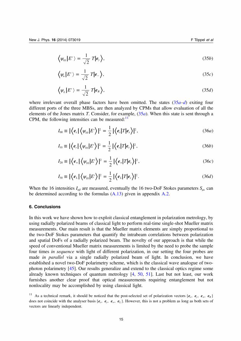
where irrelevant overall phase factors have been omitted. The states (35a–d) exiting fourdifferent ports of the three MBSs, are then analyzed by CPMs that allow evaluation of all theelements of the Jones matrix T. Consider, for example, (35a). When this state is sent through aCPM, the following intensities can be measured:11

|⟨ |⟨ | ⟩| |⟨ | | ⟩|ψ≡ =′e e eI E T a12

, (36 )x x x00 102 2

|⟨ |⟨ | ⟩| |⟨ | | ⟩|ψ≡ =′e e eI E T b12

, (36 )y y x10 102 2

|⟨ |⟨ | ⟩| |⟨ | | ⟩|ψ≡ =′+ +e e eI E T c12

, (36 )x20 102 2

|⟨ |⟨ | ⟩| |⟨ | | ⟩|ψ≡ =′e e eI E T d12

. (36 )L L x30 102 2

When the 16 intensities αβI are measured, eventually the 16 two-DoF Stokes parameters μνS canbe determined according to the formulas (A.13) given in appendix A.2.

6. Conclusions

In this work we have shown how to exploit classical entanglement in polarization metrology, byusing radially polarized beams of classical light to perform real-time single-shot Mueller matrixmeasurements. Our main result is that the Mueller matrix elements are simply proportional tothe two-DoF Stokes parameters that quantify the intrabeam correlations between polarizationand spatial DoFs of a radially polarized beam. The novelty of our approach is that while thespeed of conventional Mueller matrix measurements is limited by the need to probe the samplefour times in sequence with light of different polarization, in our setting the four probes aremade in parallel via a single radially polarized beam of light. In conclusion, we haveestablished a novel two-DoF polarimetry scheme, which is the classical wave analogue of two-photon polarimetry [45]. Our results generalize and extend to the classical optics regime somealready known techniques of quantum metrology [4, 50, 51]. Last but not least, our workfurnishes another clear proof that optical measurements requiring entanglement but notnonlocality may be accomplished by using classical light.

11 As a technical remark, it should be noticed that the post-selected set of polarization vectors +e e e e{ , , , }x y R

does not coincide with the analyser basis +e e e e{ , , , }x y L . However, this is not a problem as long as both sets ofvectors are linearly independent.

15

New J. Phys. 16 (2014) 073019 F Töppel et al

Appendix A. Qubit operations

A.1. Single-DoF operations

Consider the single-qubit two-dimensional Hilbert space = | ⟩ | ⟩ span{ 0 , 1 }1 , where thestandard basis states | ⟩0 and | ⟩1 are defined as the eigenstates of the σ3 Pauli matrix in (16),irrespective of the specific DoF encoding the qubit. All the results obtained in this appendix areindeed equally valid for both polarization and spatial qubits, as defined by (6a) and (6b).Similarly, the basis vectors | + ⟩ | − ⟩{ , } and | ⟩ | ⟩L R{ , } are defined as the eigenstates of theremaining two Pauli matrices σ1 and σ2, respectively, where

+ = + − = −a

0 1

2,

0 1

2, (A.1 )

= + = −L R b

0 i 1

2,

0 i 1

2. (A.1 )

Rotatable π- and π /2-converters permit any transformation between these basis vectors [49].According to [52], the unitary matrices representing π- and π /2-converters can be written as:

= − =ππ

ππ− −⎡

⎣⎢⎤⎦⎥

⎡⎣⎢

⎤⎦⎥U Ue 1 0

0 1, e 1 0

0 i, (A.2)i 2

2i 4

where the conventional overall phase factors are fixed by the condition that, for the polarizationqubit, the fast axes of both HWP and QWP are horizontal. The unitary matrix θφU ( ), withφ π π∈ { , /2} for a φ-converter rotated by an angle θ, is given by

θ θ θ= −φ φU D U D( ) ( ) ( ), (A.3)

where θD ( ) denotes the standard 2 × 2 rotation matrix:

θ θ θθ θ

= −⎡⎣⎢

⎤⎦⎥D ( ) cos sin

sin cos. (A.4)

For example, we can use (A.3) to transform the vectors (A.1a) and (A.1b) into the standardbasis, as follows:

π ππ π

+ = − − = −= = −

π π

π π

U U

U L U R

( 8) i 0 , ( 8) i 1 ,

( 4) 0 , ( 4) i 1 . (A.5)2 2

Consider now the four basis states | ⟩ | ⟩ |+⟩ | ⟩L{ 0 , 1 , , } that we conveniently relabel as| ⟩ | ⟩ | ⟩ | ⟩{ 0 , 1 , 2 , 3 }. From these states we can built the four linearly independent projectionmatrices μ μ≡ | ⟩⟨ |μE :

σ σ σ σ

σ σ σ σ

= =+

= =−

= =+

=

−

=+

⎡⎣⎢

⎤⎦⎥

⎡⎣⎢

⎤⎦⎥

⎡

⎣

⎢⎢⎢⎢

⎤

⎦

⎥⎥⎥⎥

⎡

⎣

⎢⎢⎢⎢

⎤

⎦

⎥⎥⎥⎥

E E

E E

1 00 0 2

, 0 00 1 2

,

12

12

12

12

2,

12

i2

i2

12

2. (A.6)

00 3

10 3

20 1

30 2

These relations can be inverted to give σ = +E E0 0 1, σ = − − +E E E21 0 1 2,σ = − − +E E E22 0 1 3, σ = −E E3 0 1 or, formally,

16

New J. Phys. 16 (2014) 073019 F Töppel et al

∑ ∑σ σ μ= = =μα

μα α μα

μα α= =

E g f Eand ( 0, 1, 2, 3), (A.7)0

3

0

3

where, from the orthogonality of the Pauli matrices it follows that σ=μα μ αg Etr ( )/2. Thecoefficients μαf can be found by noticing that the two 4 × 4 matrices F and G defined as

=μα μαG g[ ] and =μα μαF f[ ] , are connected by the simple relation = −F G 1, which implies=μα μα

−f G[ ]1 .From an operational point of view, the projector E2 can be physically implemented with a

π-converter followed by the projector E0:

π π= π†

πE U E U( 8) ( 8), (A.8)2 0

where (A.5) has been used. Similarly, the projector E3 can be realized with a π /2-converterfollowed by the projector E0:

π π= π†

πE U E U( 4) ( 4). (A.9)23 0 2

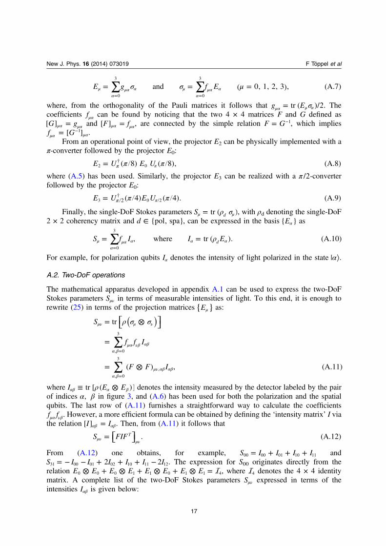
Finally, the single-DoF Stokes parameters ρ σ=μ μS tr ( )d , with ρd denoting the single-DoF2 × 2 coherency matrix and ∈d {pol, spa}, can be expressed in the basis αE{ } as

∑ ρ= =μα

μα α α α=

S f I I E, where tr ( ). (A.10)d0

3

For example, for polarization qubits αI denotes the intensity of light polarized in the state α| ⟩.

A.2. Two-DoF operations

The mathematical apparatus developed in appendix A.1 can be used to express the two-DoFStokes parameters μνS in terms of measurable intensities of light. To this end, it is enough torewrite (25) in terms of the projection matrices μ{ }E as:

∑

∑

ρ σ σ= ⊗

=

= ⊗

μν μ ν

α βμα νβ αβ

α βμν αβ αβ

=

=

⎡⎣ ⎤⎦( )S

f f I

F F I

tr

( ) , (A.11)

, 0

3

, 0

3

,

where ρ≡ ⊗αβ α βI E Etr [ ( )] denotes the intensity measured by the detector labeled by the pairof indices α β, in figure 3, and (A.6) has been used for both the polarization and the spatialqubits. The last row of (A.11) furnishes a straightforward way to calculate the coefficients

μα νβf f . However, a more efficient formula can be obtained by defining the ‘intensity matrix’ I viathe relation =αβ αβI I[ ] . Then, from (A.11) it follows that

=μν μν⎡⎣ ⎤⎦S FIF . (A.12)T

From (A.12) one obtains, for example, = + + +S I I I I00 00 01 10 11 and= − − + + + −S I I I I I I2 231 00 01 02 10 11 12. The expression for S00 originates directly from the

relation ⊗ + ⊗ + ⊗ + ⊗ = E E E E E E E E0 0 0 1 1 0 1 1 4, where 4 denotes the 4 × 4 identitymatrix. A complete list of the two-DoF Stokes parameters μνS expressed in terms of theintensities αβI is given below:

17

New J. Phys. 16 (2014) 073019 F Töppel et al

= + + += − − + − − += − − + − − += − + −= − − − − + += + − + + − + + −= + − + + − + + −= − + − + + −= − − − − + += + − + + − + + −= + − + + − + + −= − + − + + −= + − −= − − + + + −= − − + + + −= − − +

( )( )( )

( )( )( )

S I I I I

S I I I I I I

S I I I I I I

S I I I I

S I I I I I I

S I I I I I I I I I

S I I I I I I I I I

S I I I I I I

S I I I I I I

S I I I I I I I I I

S I I I I I I I I I

S I I I I I I

S I I I I

S I I I I I I

S I I I I I I

S I I I I

,2 2 ,2 2 ,

,

2 ,

2 2 2 ,

2 2 2 ,

2 2 ,

2 ,

2 2 2 ,

2 2 2 ,

2 2 ,,

2 2 ,2 2 ,

. (A.13)

00 00 01 10 11

01 00 01 02 10 11 12

02 00 01 03 10 11 13

03 00 01 10 11

10 00 01 10 11 20 21

11 00 01 02 10 11 12 20 21 22

12 00 01 03 10 11 13 20 21 23

13 00 01 10 11 20 21

20 00 01 10 11 30 31

21 00 01 02 10 11 12 30 31 32

22 00 01 03 10 11 13 30 31 33

23 00 01 10 11 30 31

30 00 01 10 11

31 00 01 02 10 11 12

32 00 01 03 10 11 13

33 00 01 10 11

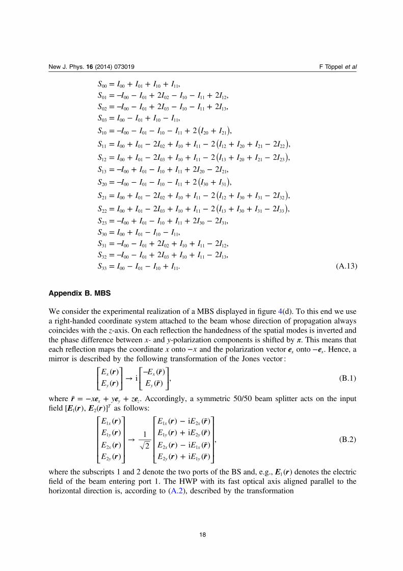
Appendix B. MBS

We consider the experimental realization of a MBS displayed in figure 4(d). To this end we usea right-handed coordinate system attached to the beam whose direction of propagation alwayscoincides with the z-axis. On each reflection the handedness of the spatial modes is inverted andthe phase difference between x- and y-polarization components is shifted by π. This means thateach reflection maps the coordinate x onto −x and the polarization vector ex onto −ex. Hence, amirror is described by the following transformation of the Jones vector :

→− ¯

¯⎡⎣⎢

⎤⎦⎥

⎡⎣⎢

⎤⎦⎥

rr

rr

E

E

E

E

( )

( )i

( )

( ), (B.1)

x

y

x

y

where ¯ = − + +r e e ex y zx y z. Accordingly, a symmetric 50/50 beam splitter acts on the inputfield E r E r[ ( ), ( )]T

1 2 as follows:

→

− ¯+ ¯− ¯+ ¯

⎡

⎣

⎢⎢⎢⎢

⎤

⎦

⎥⎥⎥⎥

⎡

⎣

⎢⎢⎢⎢

⎤

⎦

⎥⎥⎥⎥

rr

rr

r rr r

r rr r

E

E

E

E

E E

E E

E E

E E

( )

( )

( )

( )

1

2

( ) i ( )

( ) i ( )

( ) i ( )

( ) i ( )

, (B.2)

x

y

x

y

x x

y y

x x

y y

1

1

2

2

1 2

1 2

2 1

2 1

where the subscripts 1 and 2 denote the two ports of the BS and, e.g., E r( )1 denotes the electricfield of the beam entering port 1. The HWP with its fast optical axis aligned parallel to thehorizontal direction is, according to (A.2), described by the transformation

18

New J. Phys. 16 (2014) 073019 F Töppel et al

→−⎡

⎣⎢⎤⎦⎥

⎡⎣⎢

⎤⎦⎥

rr

rr

E

E

E

E

( )

( )i

( )

( ). (B.3)

x

y

x

y

As our proposal uses solely first-order spatial modes, let us consider the input fieldsψ ψ ψ ψ= + + +E r r r e r r eA A A A( ) [ ( ) ( )] [ ( ) ( )]1

inx y00 10 01 01 10 10 11 01 and =E r( ) 02

in . The MBStransforms these input fields into the output fields

ψ= − +( )E r e e rA A( ) ( ), (B.4)1out

x y00 10 10

and

ψ= +( )E r e e rA A( ) ( ). (B.5)2out

x y01 11 01

Figure B1. Visualization of the working principle of a mode beam splitter (MBS). Thenumbers 1 and 2 label the two arms of the MBS and dashed lines denote dark channels.(a–b) The horizontally and vertically polarized HG modes ψ=E r e r( ) ( )1

inx 10 and

ψ=E r e r( ) ( )1in

y 10 , are transmitted across port 1. (c–d) The horizontally and verticallypolarized HG modes ψ=E r e r( ) ( )1

inx 01 and ψ=E r e r( ) ( )1

iny 01 are transmitted across

port 2. (e) The MBS splits a radially polarized beam ψ ψ= +E r e r e r( ) [ ( ) ( )]/ 21in

x y10 01into its components ψ=E r e r( ) ( )1

outx 10 and ψ=E r e r( ) ( )2

outy 01 .

19

New J. Phys. 16 (2014) 073019 F Töppel et al

as can be shown by successively applying the transformations of each element of the MBSdescribed above. Furthermore, the fact was used that the HG mode ψ10 changes sign uponreflection, i.e. ψ ψ¯ = −r r( ) ( )10 10 , whereas this is not the case for the HG mode ψ01, i.e.ψ ψ¯ =r r( ) ( )01 01 . The action of the MBS in several input beams E1

in is visualized in figure B1.

References

[1] Massar S and Popescu S 1995 Optimal extraction of information from finite quantum ensembles Phys. Rev.Lett. 74 1259–63

[2] Gisin M 2001 Coherent quantum measurement for the direct determination of the degree of polarization andpolarization mode dispersion compensation J. Mod. Opt. 48 1397–403

[3] Abouraddy A F, Saleh B E A, Sergienko A V and Teich M C 2001 Role of entanglement in two-photonimaging Phys. Rev. Lett. 87 123602

[4] Aiello A and Woerdman J P 2004 Linear algebra for Mueller calculus Preprint (arXiv:math-ph/0412061)[5] Legré M, Wegmüller M and Gisin N 2003 Quantum measurement of the degree of polarization of a light

beam Phys. Rev. Lett. 91 167902[6] Brunner N, Acín A, Collins D, Gisin N and Scarani V 2003 Optical telecom networks as weak quantum

measurements with post-selection Phys. Rev. Lett. 91 180402[7] Gisin N 1991 Bell’s inequality holds for all non-product states Phys. Lett. 154 201–2[8] Spreeuw R J C 1998 A classical analogy of entanglement Found. Phys. 28 361–74[9] Brunner N, Gisin N and Scarani V 2005 Entanglement and non-locality are different resources New J. Phys. 7

88[10] Aspect A 1983 Experimental test of Bellʼs inequalities using time-varying analyzers Phys. Rev. Lett. 49 1804[11] Hasegawa Y, Loidl R, Badurek G, Baron M and Rauch H 2003 Violation of a Bell-like inequality in single-

neutron interferometry Nature 425 45–8[12] Souza C E R, Huguenin J A O, Milman P and Khoury A Z 2007 Topological phase for spin–orbit

transformations on a laser beam Phys. Rev. Lett. 99 160401[13] Luis A 2009 Coherence, polarization, and entanglement for classical light fields Opt. Commun. 282 3665–70[14] Holleczek A, Aiello A, Gabriel C, Marquardt C and Leuchs G 2010 Poincaré sphere representation for

classical inseparable Bell-like states of the electromagnetic field (arXiv:1007.2528)[15] Borges C V S, Hor-Meyll M, Huguenin J A O and Khoury A Z 2010 Bell-like inequality for the spin-orbit

separability of a laser beam Phys. Rev. A 82 033833[16] Karimi E et al 2010 Spin–orbit hybrid entanglement of photons and quantum contextuality Phys. Rev. A 82

022115[17] Goldin M A, Francisco D and Ledesma A 2010 Simulating Bell inequality violations with classical optics

encoded qubits J. Opt. Soc. Am. B 27 779–86[18] Qian X-F and Eberly J H 2011 Entanglement and classical polarization states Opt. Lett. 36 4110–2[19] Holleczek A, Aiello A, Gabriel C, Marquardt C and Leuchs G 2011 Classical and quantum properties of

cylindrically polarized states of light Opt. Express 19 9714–36[20] Gabriel C et al 2011 Entangling different degrees of freedom by quadrature squeezing cylindrically polarized

modes Phys. Rev. Lett. 106 060502[21] Simon B N, Simon S, Gori F, Santarsiero M, Borghi R, Mukunda N and Simon R 2010 Nonquantum

entanglement resolves a basic issue in polarization optics Phys. Rev. Lett. 104 023901[22] de Oliveira A N, Walborn S P and Monken C H 2005 Implementing the Deutsch algorithm with polarization

and transverse spatial modes J. Opt. B: Quantum Semiclass. Opt. 7 288–92[23] Goyal S K, Roux F S, Forbes A and Konrad Th 2013 Implementing quantum walks using orbital angular

momentum of classical light Phys. Rev. Lett. 110 263602

20

New J. Phys. 16 (2014) 073019 F Töppel et al

[24] Kagalwala K H, di Giuseppe G, Abouraddy A F and Saleh B E A 2013 Bellʼs measure in classical opticalcoherence Nat. Photonics 7 72–8

[25] Ghose P and Mukhrjee A 2014 Entanglement in classical optics Rev. Theor. Sci. 2 274–88[26] Mueller H 1943 Memorandum on the polarization optics of the photo-elastic shutter Report Number 2 of the

OSRD Project OEMsr-576[27] Damask J N 2005 Polarization Optics in Telecommunications (New York: Springer)[28] Le Roy-Brehonnet F and Jeune B L 1997 Utilization of Mueller matrix formalism to obtain optical targets

depolarization and polarization properties Prog. Quantum Electron. 21 109–51[29] Aiello A, Puentes G, Voigt D and Woerdman J P 2006 Maximum-likelihood estimation of Mueller matrices

Opt. Lett. 31 817–9[30] Paetz gen Schieck H 2012 Nuclear Physics with Polarized Particles (Lecture Notes in Physics vol 842)

(Berlin: Springer)[31] Clarke D 2010 Stellar Polarimetry (New York: Wiley)[32] Van Zyl J J 2011 Synthetic Aperture Radar Polarimetry (JPL Space Science and Technology Series)

(Hoboken, NJ: Wiley)[33] Tuchin V V, Wang L and Zimnyakov D A 2006 Optical Polarization in Biomedical Applications (Berlin:

Springer)[34] Schott J R 2009 Fundamentals of Polarimetric Remote Sensing (SPIE Tutorial Text vol TT81) (Washington,

DC: SPIE)[35] Firdous S 2010 Laser Tissue Interaction and Wave Propagation in Random Media: Mueller Matrix

Polarimetry (Mostbach: Physik Verlag)[36] Siegman A E 1986 Lasers (Mill Valley: University Science Books) chapter 16[37] Jones R C 1941 A new calculus for the treatment of optical systems, I. Description and discussion of the

calculus J. Opt. Soc. Am. 31 488–93[38] Padgett M J and Courtial J 1999 Poincaré-sphere equivalent for light beams containing orbital angular

momentum Opt. Lett. 24 430–2[39] Nielsen M A and Chuang I L 2010 Quantum Computation and Quantum Information (Cambridge:

Cambridge University Press)[40] Balian R 1999 Incomplete descriptions and relevant entropies Am. J. Phys. 67 1078–90[41] Mandel L and Wolf E 1995 Optical Coherence and Quantum Optics (Cambridge: Cambridge University

Press)[42] Lehner J, Leonhardt U and Paul H 1996 Unpolarized light: classical and quantum states Phys. Rev. A 53

2727–35[43] Bickel W S and Bailey WM 1985 Stokes vectors, Mueller matrices, and polarized scattered light Am. J. Phys.

53 468–78[44] James D F V, Kwiat P G, Munro W J and White A G 2001 Measurement of qubits Phys. Rev. A 64 052312[45] Abouraddy A F, Sergienko A V, Saleh B E A and Teich M C 2002 Quantum entanglement and the two-

photon Stokes parameters Opt. Commun. 201 93–8[46] Loudon R 2001 The Quantum Theory of Light 3rd edn (Oxford: Oxford University Press)[47] Beijersbergen M W, Allen L, van der Veen H E L O and Woerdman J P 1993 Astigmatic laser mode

converters and transfer of orbital angular momentum Opt. Commun. 96 123–32[48] Sasada H and Okamoto M 2003 Transverse-mode beam splitter of a light beam and its application to quantum

cryptography Phys. Rev. A 68 012323[49] Luda M A, Larotonda M A, Paz J P and Schmiegelow C T 2014 Manipulating transverse modes of photons

for quantum cryptography Phys. Rev. A 89 042325[50] Aiello A, Puentes G and Woerdman J P 2007 Linear optics and quantum maps Phys. Rev. A 76 032323[51] Toussaint K C, di Giuseppe G, Bycenski K J, Sergienko A V, Saleh B E A and Teich M C 2004 Quantum

ellipsometry using correlated-photon beams Phys. Rev. A 70 023801[52] Pedrotti F L and Pedrotti L S 1993 Introduction to Optics (Englewood Cliffs, NJ: Prentice-Hall) chapter 14

21

New J. Phys. 16 (2014) 073019 F Töppel et al