Classical and Quantum Imaging and Metrology Using Far ... · Department of Physics and Astromony...
115
Thesis submitted for the degree of Doctor of Philosophy Department of Physics and Astromony Classical and Quantum Imaging and Metrology Using Far Field Radiation Mark Edward Pearce November 16, 2015
Transcript of Classical and Quantum Imaging and Metrology Using Far ... · Department of Physics and Astromony...
Thesis submitted for the degree of
Doctor of Philosophy
Department of Physics and Astromony
Classical and Quantum
Imaging and Metrology Using
Far Field Radiation
Mark Edward Pearce
November 16, 2015

Abstract
In this thesis I examine how the statistical properties of radiation limit our abilityto perform imaging and metrological procedures. In particular I focus on radiationin the far field zone of the source. The classical and quantum theories of parame-ter estimation are introduced and subsequently utilised throughout, along with thetheory of optical coherence. Classical and quantum imaging protocols are examinedwith the aid of a resolution criterion and the criterion is shown to reproduce the re-sults of previous works. This method is also extended to previously un-investigatedsituations and the effect of imperfect measurements is explored. Intensity correla-tion measurements are investigated in great detail and for the first time a rigorouscomparison is made between higher-order intensity correlation measurements of thetype introduced by Hanbury Brown and Twiss. The importance of considering co-variances in intensity correlation data is demonstrated and I give a full, detailedaccount of how to include this in the formulation. I also show how the optimal ar-rangement for an intensity correlation measurement can be found, therefore allowingthe best precision in parameter estimation to be achieved. A quantum mechanicaldescription of blackbody radiation is used to examine the state arriving at a detectorin the far field. By using the quantum Fisher information an interesting connectionis found between the statistical independence of photons in the source plane and theacquisition of information in the far field.
iii


To William Alfred Pearce
v


Declaration of Authorship
I, Mark Edward Pearce, declare that the work presented in this thesis is my ownresearch except where otherwise stated and has not been previously submitted for adegree in this or another university. Parts of the work submitted in this thesis havebeen published as follows:
Publications
1. Carlos Perez-Delgado, Mark E. Pearce and Pieter Kok, Fundamental Limitsof Classical and Quantum Imaging, Physical Review Letters 109(12), 123601,21 September 2012.
2. Mark E. Pearce, Thomas Mehringer, Joachim von Zanthier and Pieter Kok,Precision Estimation of Source Dimensions from Higher-Order Intensity Cor-relations, Physical Review A 92, 043831, 21 October 2015.
Signed:
Dated:
vii

Acknowledgements
Firstly, I would like to thank my supervisor, Pieter Kok for continued support andencouragement throughout my university education and research career. He hasbeen a fantastic teacher and a truly inspirational influence. I certainly could nothave completed this research without his guidance.
I would like to thank my friends and colleagues with whom I have shared an of-fice whilst working towards my PhD; Carl Whitfield, Emiliano Cancellieri, MichaelWoodhouse, Ian Estabrook, Jasminder Sidhu, Dominic Hostler, Earl Campbell,Giuseppe Buonaiuto, and Tom Bullock. They have been a great source of inspi-ration and it has been a pleasure to work alongside so many talented physicists. Aspecial thank you is reserved for Samuel Coveney for teaching me the CUDA pro-gramming language, which proved essential in my research and I am therefore hugelygrateful. Thanks is also due to Nigel Clarke for allowing me to use his computingequipment, without which I could not have performed my research.
I would also like to extend a huge thank you to my family and friends who havesupported and encouraged me throughout my time at university. I am grateful tomy parents, Angela and Ed, and my sister Kate, who have been both loving andsupportive throughout my studies. My partner Helen is also due a special thankyou, her patience and understanding have been crucial in me finishing this work.
I am thankful to Prof. Joachim von Zanthier, Steffen Oppel, and Thomas Mehringerfor their ongoing collaboration. Their work has been instrumental in the develop-ment of my ideas and their hospitality during our visit to Erlangen was greatlyappreciated.
ix


Contents
1 Introduction 1
2 Quantum Optics 52.1 The quantum electromagnetic field . . . . . . . . . . . . . . . . . . . 52.2 States of the electromagnetic field . . . . . . . . . . . . . . . . . . . . 82.3 Optical coherence . . . . . . . . . . . . . . . . . . . . . . . . . . . . . 132.4 Quantum theory of coherence . . . . . . . . . . . . . . . . . . . . . . 152.5 The Gaussian moment theorem . . . . . . . . . . . . . . . . . . . . . 182.6 Correlations in the far field . . . . . . . . . . . . . . . . . . . . . . . . 212.7 The Rayleigh diffraction formula . . . . . . . . . . . . . . . . . . . . . 222.8 Monochromatic approximation . . . . . . . . . . . . . . . . . . . . . . 24
3 Estimation Theory 253.1 Classical estimation theory . . . . . . . . . . . . . . . . . . . . . . . . 25
3.1.1 The Cramer-Rao bound . . . . . . . . . . . . . . . . . . . . . 263.1.2 The multi-parameter Cramer-Rao bound . . . . . . . . . . . . 293.1.3 Estimating parameters . . . . . . . . . . . . . . . . . . . . . . 31
3.2 Quantum estimation theory . . . . . . . . . . . . . . . . . . . . . . . 323.2.1 The quantum Fisher information . . . . . . . . . . . . . . . . 323.2.2 The multi-parameter quantum Cramer-Rao bound . . . . . . . 35
4 Fundamental Limits of Classical and Quantum Imaging 374.1 Positive Operator Valued Measures . . . . . . . . . . . . . . . . . . . 374.2 Image resolution . . . . . . . . . . . . . . . . . . . . . . . . . . . . . 384.3 The imaging observable . . . . . . . . . . . . . . . . . . . . . . . . . . 384.4 Examples . . . . . . . . . . . . . . . . . . . . . . . . . . . . . . . . . 414.5 Detector imperfections . . . . . . . . . . . . . . . . . . . . . . . . . . 454.6 Multi-photon correlations . . . . . . . . . . . . . . . . . . . . . . . . 51
4.6.1 Single photon sources . . . . . . . . . . . . . . . . . . . . . . . 534.6.2 Thermal light sources . . . . . . . . . . . . . . . . . . . . . . . 54
4.7 Discussion and conclusions . . . . . . . . . . . . . . . . . . . . . . . . 56
5 Estimation of Thermal Source Dimensions 575.1 n-point intensity correlation functions . . . . . . . . . . . . . . . . . . 595.2 Estimation from intensity correlations . . . . . . . . . . . . . . . . . . 625.3 Measuring the correlation functions . . . . . . . . . . . . . . . . . . . 645.4 Numerical Simulations . . . . . . . . . . . . . . . . . . . . . . . . . . 66
5.4.1 Constant detector loss . . . . . . . . . . . . . . . . . . . . . . 685.4.2 Detector loss as a random variable . . . . . . . . . . . . . . . 69
xi
xii CONTENTS
5.5 Discussion and conclusions . . . . . . . . . . . . . . . . . . . . . . . . 71
6 Obtaining Spatial Information From Far Field Sources 756.1 Blackbody radiation . . . . . . . . . . . . . . . . . . . . . . . . . . . 756.2 Frequency mode representation of ρ . . . . . . . . . . . . . . . . . . . 776.3 The quantum Fisher information for blackbody radiation . . . . . . . 796.4 Spatially separated sources . . . . . . . . . . . . . . . . . . . . . . . . 846.5 The spatial wavefunction φn(y1, . . . ,yn) . . . . . . . . . . . . . . . . 856.6 Alternative method . . . . . . . . . . . . . . . . . . . . . . . . . . . . 886.7 Discussion and conclusions . . . . . . . . . . . . . . . . . . . . . . . . 89
7 Summary and Outlook 91
A Quasi-Probability Distributions in Quantum Optics 93
B Moments of the Noise Distribution 95

Chapter 1
Introduction
Imaging plays a fundamental role in science and technology. Historically, everytime a new imaging technique was introduced, science has leaped forward. For ex-ample, recent imaging applications include exoplanet detection [Macintosh et al.,2014] and the velocity measurement of molecular markers along DNA [Heller et al.,2013]. When examining imaging instruments it is of particular importance that wecan characterise their resolution. The resolution of an imaging procedure quanti-fies the finest details we can distinguish on the object we are imaging. The wavenature of light dictates that there are physical limits to the resolution of opticalmicroscopes and telescopes. In order to see smaller details in microscopy we couldilluminate with light of shorter and shorter wavelengths, but this is not always prac-tical: increasingly energetic light may destroy biological samples, and in astronomythe accessible wavelengths are beyond our control. We therefore need to find alter-native techniques to improve the resolution of our imaging methods that overcomethe diffraction limit. The first attempts to determine the resolution of an imagingprocedure were given by Rayleigh [Rayleigh, 1879] and Abbe [Abbe, 1873]. BothAbbe and Rayleigh defined resolution phenomenologically as the ability for observersto distinguish two overlapping intensity distributions. By defining resolution in thisway, taking into account only the expectation value of the intensity across the imageplane, the statistical nature of the measured intensity is ignored. Since statisticalfluctuations are present in almost all physical systems, a full characterisation ofthe resolution of an imaging system must take these effects into account. Imag-ing techniques that yield finer detail than that dictated by the Rayleigh and Abbelimits are referred to as super-resolving techniques. In microscopy techniques suchas photo-activated localised microscopy (palm) [Hess et al., 2006], stochastic opti-cal reconstruction microscopy (storm) [Rust et al., 2006] and stimulated-emissiondepletion microscopy (sted) [Hell and Wichmann, 1994] achieve super-resolved im-ages using fluorescent markers. These methods combine standard intensity mea-surements with prior information about the sample preparation and post-processingto achieve super-resolution. In the year 2000 Pendry developed a new theoreticalmethod of super-resolution that involved using materials of negative refractive in-dex as lenses [Pendry, 2000]. In this paper, Pendry shows that a lens made of amaterial with a refractive index of −1 is theoretically capable of producing perfectimages that are not limited by diffraction. In practice, materials that exhibit re-fractive indexes of −1 are difficult to manufacture. They also tend to suffer fromhigh dispersion, which limits there resolving power in practice. In this thesis we
1
2
use the rigorous method of parameter estimation theory to define the resolution ofthe systems we investigate. The success of classical theories in describing opticalphenomena meant that the introduction of quantum mechanical methods was slowto be adopted by the optical community. Eventually though, the quantum natureof light was subtly revealed and a new branch of quantum physics was established.
The development of quantum optics began in the late 1950’s, sparked by thediscovery of a new type of interferometer by Hanbury Brown and Twiss [Brown andTwiss, 1956a, Brown and Twiss, 1956b, Brown and Twiss, 1957, Brown and Twiss,1958a,Brown and Twiss, 1958b,Brown and Twiss, 1958c]. They called this new typeof interferometer an intensity interferometer, and initially it appeared that there wasa discrepancy between the classical and quantum theories describing the workings ofthe device. The classical description given by Hanbury Brown and Twiss correctlypredicted the experimental observations [Brown and Twiss, 1956b] whilst otherssuggested that if their experimental results were correct, the quantum theory of thephoton would require elaboration [Brannen and Ferguson, 1956]. Purcell was oneof few researchers who strongly believed that the effect would adhere to a quantumdescription and was the first to give a successful quantum analysis of the effect interms of the “clumping” of bosons [Purcell, 1956,Silva and Freire Jr, 2013].
Although the effect discovered by Hanbury Brown and Twiss was successfully ex-plained by a completely classical theory, the debate surrounding the validity of theirresults compelled researchers to develop the currently existing classical discipline ofoptics into a fully fledged quantum theory [Gerry and Knight, 2006,Walls and Mil-burn, 2008,Glauber, 2007]. Among the developments spurred by the experiments ofHanbury Brown and Twiss were the seminal works of Glauber on the quantum the-ory of optical coherence [Glauber, 1963a,Glauber, 1963c,Glauber, 1963b]. Glauber’stheory could successfully explain the effects observed in the experiments of HanburyBrown and Twiss and could also explain the coherence phenomena that were ob-served in all optics experiments prior to this. The modern theory of optical coherenceas pioneered by Glauber, characterises the phenomenon with a set of functions in-dexed by a pair of positive integers, (n,m). A complete description of the opticalfield can only be given if the functions are known for all pairs of indices. Beforethe discovery of intensity interferometry by Hanbury Brown and Twiss (HBT) alloptical experiments that relied on coherence exploited only first order coherences,that is, coherences that can be explained by the lowest order coherence function,n = m = 1.
Despite the discovery of higher order coherences taking place over fifty yearsago, relatively little work has been performed that requires the use of coherencefunctions beyond the first order. In recent years research that exploits the higherorder coherences of optical fields has become more prevalent. In the field of quan-tum computation the problem of boson sampling is one such example [Aaronsonand Arkhipov, 2010, Aaronson and Arkhipov, 2013]. The boson sampling problemrequires the calculation of high order photon coincidences and therefore relies onthe theory of higher order coherences. It is easy to show that the output of anm port interferometer, interfering n bosons, is inefficient to simulate on a classicalcomputer [Gard et al., 2014b,Motes et al., 2013]. It is unclear whether the presenceof noise will affect this result making the distribution efficiently classically simu-lated [Gogolin et al., 2013,Aaronson and Arkhipov, 2013]. It is for this reason thatresearchers in this area anticipate that a boson sampling machine may be useful in

CHAPTER 1. INTRODUCTION 3
implementing quantum computational tasks. However, to date no known use of aboson sampling machine exists [Gard et al., 2014a]. 1
In 1995 Pittman et al., inspired by the work of Klyshko [Klyshko, 1988], de-veloped an imaging technique that would later become known as ghost imaging[Pittman et al., 1995]. Their technique uses a pair of correlated photons, producedvia spontaneous parametric down-conversion, one of which is directed towards anobject and then recorded by a detector that does not spatially resolve the pres-ence of the photon, the other is not directed towards the object but is measuredby a spatially resolving detector. By measuring the coincidence counts of the twophotons, a spatially resolved image of the object is obtained despite the spatial in-formation only being obtained for the photon that did not interact with the object.The photons produced by spontaneous parametric downconversion are highly en-tangled and therefore exhibit a strong type of correlation that can only be observedin quantum systems. Classical systems can also exhibit correlations, and pairs ofclassically correlated photons can also be used to perform ghost imaging [Benninket al., 2002,Ferri et al., 2005,Gatti et al., 2006]. Generally, the price paid for usingthe weaker correlations present in classical systems instead of the stronger quantumcorrelations, is a decrease in the visibility of the ghost image [Gatti et al., 2007].Since ghost imaging measures the two photon coincidence rate, it is closely related tothe measurements of Hanbury Brown and Twiss and again requires the use of higherorder coherence theory to correctly predict the outcome. More recently, researchershave started to examine generalisations of the ghost imaging protocol in which anm+n coincidence is measured, m being the number of non-spatially resolving coinci-dences measured and n being the number of spatially resolving detectors [Agafonovet al., 2009a, Agafonov et al., 2009b, Chan et al., 2009, Chen et al., 2010, Liu et al.,2009]. The use of higher order coincidences can lead to an increase in the visibilityof the ghost image. However, generally the signal to noise ratio decreases as thecoincidence order is increased.
Higher order correlations can also be exploited in generalisations of the originalHanbury Brown and Twiss experiments [Cao et al., 2008,Agafonov et al., 2008a,Liuand Shih, 2009, Zhou et al., 2010]. Hanbury Brown and Twiss (HBT) in theirseminal experiments demonstrated that the second order intensity correlation func-tion is proportional to the Fourier transform of the intensity distribution of thesource [Brown and Twiss, 1956a]. More generally we can measure the coincidencesbetween n photo-detectors, which also conveys information about the Fourier trans-form of the source. We call this kind of measurement an nth-order intensity corre-lation measurement since it is implemented by measuring the correlation between nintensities. The visibility of the measurements can also increase by going to highercorrelation orders but just as in the ghost imaging regime the signal to noise ratiosuffers as a result. Until now it was unclear what, if any, advantage higher ordercorrelations could offer in measurements of this type. In this thesis we explicitlycalculate the performance of estimators in the Hanbury Brown-Twiss (HBT) setupand determine how different correlation orders perform in a parameter estimation
1Shortly after the submission of this thesis, Huh et al. published a proposal for simulatingmolecular vibronic spectra using boson sampling [Huh et al., 2015]. The proposed scheme uses ageneralised version of boson sampling whereby the input states are squeezed coherent and squeezedvacuum states and allows the vibonic spectra of molecules to be determined by the output of alinear optical network. No known classical algorithms can efficiently predict these spectra.
4
similar to the original HBT measurement. To ensure the optimal performance ofsuch techniques it is necessary to obtain the best estimates possible.
Measurements of the HBT type rely on the phenomenon of photon bunching, aneffect caused by the bosonic nature of photons. Although it has been shown that theeffect of bunching can occur for statistically independent photons originating fromtwo independent atoms [Fano, 1961], we demonstrate in this thesis that imagingof thermal sources relies on the correlations present between the photons in thesource plane. In fact, we find in that in general the statistical independence of thephotons prevents us from performing the most general parameter estimation taskand therefore cannot be the source of information in HBT type measurements.
This thesis is composed of six chapters. In chapter 2 we give the theoretical back-ground to the various techniques of quantum optics that shall be used throughoutthis thesis. In particular we focus on the theory of optical coherence as developed byGlauber and we also demonstrate how propagation affects the coherence propertiesof optical fields.
In chapter 3 we give an overview of the field of parameter estimation in boththe classical and quantum regime. Particular attention is paid to the Cramer-Raobound, which is used extensively throughout the remainder of this thesis.
Chapter 4 investigates fundamental limitations placed upon imaging protocols byconsidering images as probability distributions to be discriminated. In this chapterwe also determine the effects of detector imperfections on the imaging performanceand show how the effect of any imperfection can be calculated. We end this chapterby examining multi-photon correlation experiments, enquiring as to their potentialin increasing resolution for imaging.
In chapter 5 we explicitly perform a parameter estimation procedure makinguse of data that simulates nth-order intensity correlation measurements. We makecomparisons of the estimation precision for different correlation orders and determinehow we can optimise an experiment to achieve the highest precision.
In chapter 6 we use the quantum mechanical description of a source emittingblack body radiation to determine the way in which information regarding the spatialdistribution of the source is conveyed to the far field. We show how these resultscan in principle lead to a complete calculation of the quantum Fisher information.
Chapter 7 summarises the main results of the thesis and gives the direction offuture research leading on from this work.
Chapter 2
Quantum Optics
In this chapter we introduce a fully quantum mechanical description of the electro-magnetic field and discuss some of the states of this field to be used in the forth-coming chapters. We then discuss the concept of optical coherence, first classicallyand then again using the quantum mechanical formalism of Glauber. Finally wedemonstrate how correlations in the field propagate, obtaining expressions for thecoherence properties of optical fields far from the radiation sources.
2.1 The quantum electromagnetic field
Classically, the electric field inside a volume of side lengths Lx, Ly, Lz may onlyexist in certain allowable vibrational modes, known as the modes of the cavity. Thisrestriction results from the necessity for the electric field to vanish at the edges of thecavity. We therefore require that any valid electric field inside the cavity fulfils thiscondition. From Fourier analysis we know that any such function can be expressedas
E(r, t) =∞∑
l=0
∞∑
n=0
∞∑
m=0
[Elnmalnmulnm(r, t) + E∗lnma∗lnmu∗lnm(r, t)] , (2.1)
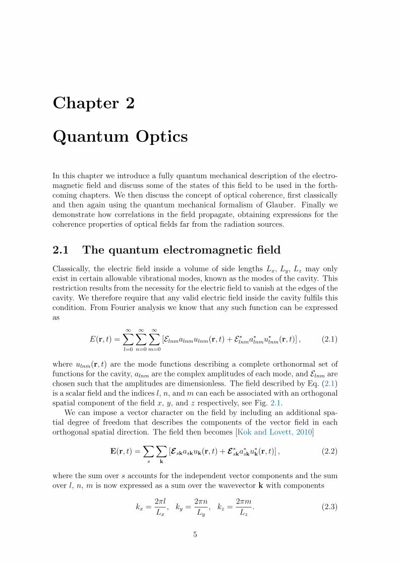
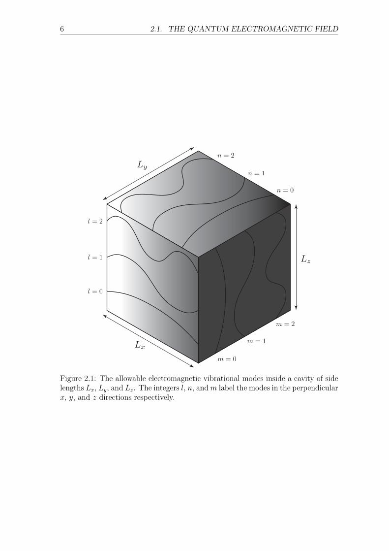
where ulnm(r, t) are the mode functions describing a complete orthonormal set offunctions for the cavity, alnm are the complex amplitudes of each mode, and Elnm arechosen such that the amplitudes are dimensionless. The field described by Eq. (2.1)is a scalar field and the indices l, n, and m can each be associated with an orthogonalspatial component of the field x, y, and z respectively, see Fig. 2.1.
We can impose a vector character on the field by including an additional spa-tial degree of freedom that describes the components of the vector field in eachorthogonal spatial direction. The field then becomes [Kok and Lovett, 2010]
E(r, t) =∑
s
∑
k
[Eskaskuk(r, t) + E∗ska∗sku∗k(r, t)] , (2.2)
where the sum over s accounts for the independent vector components and the sumover l, n, m is now expressed as a sum over the wavevector k with components
kx =2πl
Lx, ky =
2πn
Ly, kz =
2πm
Lz. (2.3)
5
6 2.1. THE QUANTUM ELECTROMAGNETIC FIELD
Figure 2.1: The allowable electromagnetic vibrational modes inside a cavity of sidelengths Lx, Ly, and Lz. The integers l, n, andm label the modes in the perpendicularx, y, and z directions respectively.
CHAPTER 2. QUANTUM OPTICS 7
The vectorial character of the field E is incorporated into the term Eλk. The field Eis now a classical vector field that obeys Maxwell’s equations and the wave equationin free space and in the absence of sources [Jackson, 1999]
∇2E(r, t)− 1
c2
∂2E(r, t)
∂t2= 0. (2.4)
where ∇2 =(∂2
∂x2, ∂
2
∂y2, ∂
2
∂z2
)is the Laplace operator.
In order to quantise the field E, the mode amplitudes ask, which have so farbeen complex numbers, now become operators. We denote this by the symbol ·.The quantised electric field is now given by
E(r, t) =∑
s
∑
k
[Eskaskuk(r, t) + E∗ska
†sku∗k(r, t)
], (2.5)
where a†sk is the Hermitian conjugate of the operator ask. The operators a†sk andask are the mode operators of the field and, as is implicit in Eq. (2.5), they arenot Hermitian. The electric field is a bosonic field and therefore the field operatorsa†sk, ask obey the bosonic commutation relations [Walls and Milburn, 2008]
[ask, a
†s′k′
]= δs,s′δk,k′ , (2.6)
and[a†sk, a
†s′k′
]= [ask, as′k′ ] = 0. (2.7)
For convenience we shall write the electric field E as the sum of two terms
E(r, t) = E(+)(r, t) + E(−)(r, t), (2.8)
where
E(+)(r, t) =∑
s
∑
k
Eskaskuk(r, t), (2.9)
and E(−) = (E(+))†. Combining Eqs. (2.4) and (2.5) we see that the mode functionsthemselves obey the wave equation and are therefore completely determined by theclassical Maxwell theory. For the cavity previously defined, the appropriate modefunctions are the plane wave modes [Walls and Milburn, 2008]
uk(r, t) =1√V
ei(k·r−ωkt), (2.10)
where ωk = c|k| and V = LxLyLz. The mode functions form a complete orthonormalset, which can be seen by taking
∫
V
dru∗k(r, t)uk′(r, t) =1
V
∫
V
d3r ei(k−k′)·r−i(ωk−ωk′ )t
= δ3(k− k′). (2.11)
The mode operators play an important role in quantum optics. For reasonsthat will become apparent, the operators a† and a are referred to as the creation
8 2.2. STATES OF THE ELECTROMAGNETIC FIELD
and annihilation operators, respectively. From Eq. (2.9) and the relation E(−) =(E(+))†, we see that the operators E(−) and E(+) are proportional to the creationand annihilation operators respectively.
Taking the limit Lx, Ly, Lz →∞, the plane wave mode functions extend over allof space-time and are therefore unphysical as a description of an observable state.We can use superpositions of the plane wave modes to effectively “localise” theelectric field modes to regions of space-time. These localised modes are referred toas wave packets and can also form complete orthonormal sets.
2.2 States of the electromagnetic field
We now present some of the more commonly used bases to describe the state ofthe electromagnetic field and discuss some of their properties. As with all quantumsystems, any basis may be used to express the state. However, certain problemsbecome much simpler when expressed in a particular choice of basis. The procedureof quantisation has the effect of discretising the electric field. As such, the fieldcannot be incrementally increased and can only increase by certain finite amounts.These amounts are the quanta of the field, in the case of the electromagnetic fieldthese quanta are known as photons. A convenient basis that reflects this quantisationis the Fock basis, also referred to as the number basis. Classically, the Hamiltoniandensity is given by [Kok and Lovett, 2010]
H =ε0
2E · E +
1
2µ0
B ·B, (2.12)
which gives the total energy of the electromagnetic field. By substituting the quan-tum mechanical form for the electric field, Eq. (2.5), making use of the relationB = 1
ωk × E, and taking the integral over the entire volume V , we arrive at the
total energy, or Hamiltonian operator,
H =
∫
V
[ε0
2E2 +
1
2µ0
B2
]d3r
=∑
s
∑
k
~ωk
[a†skask +
1
2
]. (2.13)
To elucidate the role of the operators a†sk and ask we write the eigenvalue equation
for the Hamiltonian as H|n〉 = En|n〉 and then evaluate
Ha†s′k′ |n〉 =∑
s
∑
k
~ωk
[a†skask +
1
2
]a†s′k′|n〉
=∑
s
∑
k
~ωk
[a†sk(δs,s′δk,k′ + a†s′k′ ask) +
a†s′k′
2
]|n〉
= a†s′k′
[~ωk′ +
∑
s
∑
k
~ωk
(a†skask +
1
2
)]|n〉
= (~ωk′ + En)a†s′k′ |n〉, (2.14)
where we have used Eqs. (2.6) and (2.7). Eq. (2.14) demonstrates that the statea†s′k′|n〉 is also an eigenstate of the Hamiltonian with eigenvalue En+~ωk′ . Similarly,
CHAPTER 2. QUANTUM OPTICS 9
we find that the state as′k′ |n〉 is an eigenstate of the Hamiltonian with eigenvalueEn − ~ωk′ . It is for this reason that the operators a†s′k′ and as′k′ are referred toas the creation and annihilation operators, since they fulfil the role of adding andsubtracting an amount of energy equal to ~ωk′ from the system. This is the basis ofthe quantum theory of light.
We notice from Eq. (2.13) that the total energy is the sum of operators of theform ~ωk[a†skask + 1/2]. The total energy is therefore the sum of the energy foreach mode. Concentrating on a single mode, we can drop the subscripts ks andwrite the energy of a single mode as ~ω[a†a + 1/2]. We now see that the operatora†a is proportional to the single mode energy operator. We therefore expect theeigenstates to be the same for both operators. We write
a†a|n〉 = n|n〉, (2.15)
multiplying by ~ω and adding 12~ω|n〉 we find
~ωa†a|n〉 +1
2~ω|n〉 = ~ω
(n+
1
2
)|n〉. (2.16)
The eigenvalue of the operator a†a is therefore equal to the number of photons in thestate. We therefore refer to this operator as the number operator and often write itas a†skask = nsk. The eigenstates |n〉 form a complete orthonormal set
〈n|m〉 = δn,m. (2.17)
The effect of creation and annihilation operators on the state |n〉 can now be de-termined. Since the annihilation operator destroys a photon, the action of theannihilation operator on the state |n〉 will be [Gerry and Knight, 2006]
a|n〉 ∝ |n− 1〉 (2.18)
⇒ a|n〉 = kn|n− 1〉.
To determine the constant of proportionality kn, which is potentially complex dueto the non-Hermitian nature of a, we multiply Eq. (2.18) on the left by its complexconjugate
(a|n〉)†a|n〉 = 〈n|a†a|n〉 = 〈n|n|n〉 = n〈n|n〉 = n = |kn|2. (2.19)
We therefore have the freedom to choose the phase of kn and the usual choiceis kn =
√n. From the above relation 〈n|a†a|n〉 = n we see that n is positive.
We also find the self-evident relation a|0〉 = 0, which asserts the impossibility ofhaving states with negative photon number. By performing the same calculation asEq. (2.19) with a†|n〉 we arrive at the pair of relations
a|n〉 =√n|n− 1〉 (2.20)
a†|n〉 =√n+ 1|n+ 1〉. (2.21)
And we see explicitly that the operators a† and a play the role of creating andannihilating photons.
Another important state of the electromagnetic field is the thermal state. Unlikethe number states, the thermal state is not a state of definite photon number. The

10 2.2. STATES OF THE ELECTROMAGNETIC FIELD
thermal state is also not a pure state and therefore cannot be described by a statevector |ψ〉 but must instead be written as a density operator ρ. Density operatorsdescribe mixed states, which are quantum states with classical statistical uncertain-ties as opposed to purely quantum uncertainty. To demonstrate the necessity forthe density operator formalism we consider the expectation value of an operator O
〈O〉 = 〈ψ|O|ψ〉 =n∑
i=1
〈ψ|i〉〈i|O|ψ〉 =n∑
i=1
〈i|O|ψ〉〈ψ|i〉 = Tr[O|ψ〉〈ψ|], (2.22)
where we have used the complete orthonormal basis |i〉 and Tr[·] denotes the traceoperation. The statistical uncertainty in our state manifests itself as a statisticaluncertainty of the expectation value. Moreover, if the state is a statistical mixtureof states |ψj〉 with probability pj, the expectation value will be
〈O〉 =∑
j
pjTr[O|ψj〉〈ψj|] = Tr
[∑
j
pj|ψj〉〈ψj|O]≡ Tr[ρO], (2.23)
where we have used the linearity of the trace operation and defined ρ =∑
j pj|j〉〈j|.Eq. (2.23) shows how expectation values are calculated using the density opera-tor. The density operator for any physical state must satisfy the following threeconditions [Holevo, 2011]
Tr[ρ] = 1, (2.24a)
ρ† = ρ, (2.24b)
ρ ≥ 0. (2.24c)
For a state in thermal equilibrium, the density operator is given by [Fano, 1957]
ρ =exp
(−βH
)
Tr[exp
(−βH
)] , (2.25)
where β = 1/kBT . Using Eq. (2.13) we find
ρ =exp
(−∑s,k β~ωk(nsk + 1
2))
Tr[exp
(−∑s′,k′ β~ωk′(ns′k′ + 1
2))] =
exp(−∑s,k β~ωknsk
)
Tr[exp
(−∑s′,k′ β~ωk′ns′k′
)] . (2.26)
Since 〈m|f(n)|n〉 = f(n)δn,m, any operator that is a function of the number operatoris diagonal in the number basis. We therefore evaluate the density operator in thenumber basis. First we evaluate the denominator, which, being the trace of an
CHAPTER 2. QUANTUM OPTICS 11
operator (i.e. a number), is the normalisation of the state ρ
Tr
[exp
(−∑
s′,k′
β~ωk′ns′k′
)]=∏
s,k
∑
nsk
〈nsk|exp
(−∑
s′,k′
β~ωk′ns′k′
)|nsk〉
=∏
s,k
∑
nsk
〈nsk|∏
s′,k′
exp (−β~ωk′ns′k′) |nsk〉
=∏
s,k
∑
nsk
∏
s′,k′
exp (−β~ωk′ns′k′) δs,s′δk,k′〈nsk|nsk〉
=∏
s,k
∑
nsk
exp (−β~ωknsk)
=∏
s,k
1
1− e−β~ωk. (2.27)
Therefore, the density operator is
ρ =⊗s,kexp (−β~ωknsk)∏s′,k′(1− e−β~ωk′ )−1
= ⊗s,k∑
nsk
(1− e−β~ωk)exp (−β~ωknsk) |nsk〉〈nsk|
= ⊗s,k∑
nsk
(1− e−β~ωk)exp (−β~ωknsk) |nsk〉〈nsk|, (2.28)
from which we see directly that the density operator takes the form, ρ = ⊗s,kρsk.The density operator for a thermal state naturally separates into a product overdensity operators associated with each mode. Another useful form for ρ comes fromevaluating 〈nsk〉
〈nsk〉 = Tr
[∑
nsk
(1− e−β~ωk)exp (−β~ωknsk) nsk|nsk〉〈nsk|]
=∑
nsk
(1− e−β~ωk)exp (−β~ωknsk)nsk
=1
eβ~ωk − 1. (2.29)
We now find
e−β~ωk =〈nsk〉
1 + 〈nsk〉, (2.30)
and therefore
ρsk =∑
n
〈nsk〉n(1 + 〈nsk〉)n+1
|n〉〈n|. (2.31)
It is interesting to note at this point that the density operator ρ depends only onone parameter, namely the temperature T .
For reasons that will become clear later, the thermal state is often described asincoherent radiation. In contrast, there exists another state of the electromagnetic
12 2.2. STATES OF THE ELECTROMAGNETIC FIELD
field known as the coherent state. Coherent states play a particularly importantrole in quantum optics as they are the eigenstates of the annihilation operator andare also the output states of a laser operating well above threshold [Barnett andRadmore, 1997]. Unlike thermal states, coherent states are pure and therefore donot require the density operator formalism. In the number basis the coherent stateis written as
|α〉 = e−|α|22
∞∑
n=0
αn√n!|n〉, (2.32)
where α is a complex number. With the use of Eq. (2.20) this gives
a|α〉 = e−|α|22
∞∑
n=0
αn√n!a|n〉
= e−|α|22
∞∑
n=0
αn√n!
√n|n− 1〉
= e−|α|22
∞∑
n=1
αn√(n− 1)!
|n− 1〉
= αe−|α|22
∞∑
n=0
αn√n!|n〉
= α|α〉. (2.33)
An important feature of the coherent states is the so called over-completeness. Wemight expect that the generalisation of the completeness relation to the continuousvariable α to be
∫|α〉〈α| d2α = I, however, because of the over-completeness of the
states |α〉 this requires modification [Barnett and Radmore, 1997]. Writing α = reiφ
and using Eq. (2.32), we find
∫|α〉〈α| d2α =
∫ ∞
0
r dr
∫ 2π
0
dφ e−r2∞∑
n,m=0
rn+m eiφ(n−m)
√n!m!
|n〉〈m| (2.34a)
= 2π
∫ ∞
0
r dr e−r2∞∑
n,m=0
rn+m δn,m√n!m!
|n〉〈m| (2.34b)
= 2π∞∑
n=0
∫ ∞
0
r dr e−r2 r2n
n!|n〉〈n| (2.34c)
= π
∞∑
n=0
|n〉〈n| (2.34d)
= πI, (2.34e)
where we have used the definition of the Kronecker delta in Eq. (2.34b) and thestandard integral
∫∞0
exp(−ar2)rn dr = k!/(2ak+1), n = 2k + 1, k ∈ Z, a > 0 .This proves that
1
π
∫|α〉〈α| d2α = I, (2.35)
CHAPTER 2. QUANTUM OPTICS 13
which is a consequence of the over-completeness of the coherent states |α〉.Another interesting and useful consequence of the over-completeness is that any
traceable operator O can be expressed in the coherent state basis using only thematrix elements 〈α|O|α〉 [Jordan, 1964], the over-completeness of |α〉 allowing it toprobe the off diagonal elements of O. The representation of operators in this formis known as the diagonal coherent state representation or the P -representation. Theoperator O is expressed in terms of the P -representation by
O =
∫P (α)|α〉〈α| d2α , (2.36)
where P (α) is a quasi-probability distribution which determines the weighting of theoperator O across the complex α plane. Using Eq. (2.36) we can express the densityoperator in the P -representation, in this form evaluation of expectation values isreduced to integration, sometimes simplifying the problem (see appendix A). Wewill make use of this representation later when evaluating expectation values. Wenote in passing that the coherent states presented here are part of a broader class ofgeneralised coherent states, which can be constructed for an arbitrary Lie algebra,all of which share the over-completeness property [Perelomov, 1986].
2.3 Optical coherence
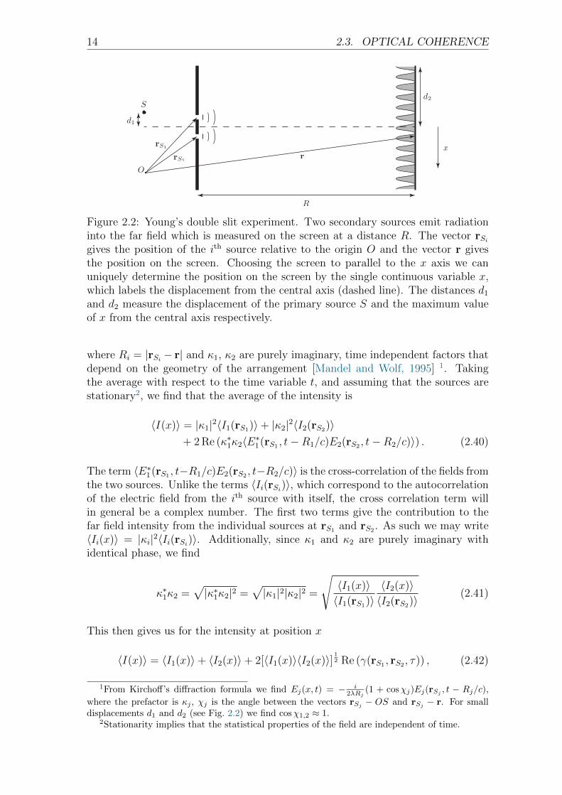
The concept of optical coherence is closely related to the concept of statistical cor-relation. When we measure radiation, we typically only come to certain statisticalconclusions. Whether the statistical uncertainties come from the inability to char-acterise the huge number of interactions in the system, such as for thermal light, orwhether it is due to fundamental quantum uncertainties, such as trying to measurethe coherent state in the Fock basis, these uncertainties are almost always present.We begin by examining optical coherence for classical fields and then develop thetheory for quantum fields. The most famous experiment demonstrating opticalcoherence is Young’s double slit experiment. The simplicity of the experimental ar-rangement allows for a simple yet effective description to be made. Consider Young’sarrangement, with two secondary sources of radiation and a screen some distance Raway on which to measure the intensity, see Fig. 2.2. The instantaneous intensity ofthe light on the screen as a function of the transverse coordinate x is given by themodulus squared of the electric field
I(x, t) = |E(x, t)|2. (2.37)
Due to the superposition principle [Hecht and Zajac, 1980], the electric field at thepoint (x, t) is the sum of the fields from the two sources
I(x, t) ∝ |E1(x, t) + E2(x, t)|2 , (2.38)
where the subscript in Ei denotes that the field originated in source i. Assumingthat the sources are point-like, producing spherical waves, we can simply relate thefields in Eq. (2.38) to the fields emitted in the source plane at earlier points intime [Born and Wolf, 1980]
I(x, t) = |κ1E1(rS1 , t−R1/c) + κ2E2(rS2 , t−R2/c)|2 , (2.39)
14 2.3. OPTICAL COHERENCE
Figure 2.2: Young’s double slit experiment. Two secondary sources emit radiationinto the far field which is measured on the screen at a distance R. The vector rSigives the position of the ith source relative to the origin O and the vector r givesthe position on the screen. Choosing the screen to parallel to the x axis we canuniquely determine the position on the screen by the single continuous variable x,which labels the displacement from the central axis (dashed line). The distances d1
and d2 measure the displacement of the primary source S and the maximum valueof x from the central axis respectively.
where Ri = |rSi − r| and κ1, κ2 are purely imaginary, time independent factors thatdepend on the geometry of the arrangement [Mandel and Wolf, 1995] 1. Takingthe average with respect to the time variable t, and assuming that the sources arestationary2, we find that the average of the intensity is
〈I(x)〉 = |κ1|2〈I1(rS1)〉+ |κ2|2〈I2(rS2)〉+ 2 Re (κ∗1κ2〈E∗1(rS1 , t−R1/c)E2(rS2 , t−R2/c)〉) . (2.40)
The term 〈E∗1(rS1 , t−R1/c)E2(rS2 , t−R2/c)〉 is the cross-correlation of the fields fromthe two sources. Unlike the terms 〈Ii(rSi)〉, which correspond to the autocorrelationof the electric field from the ith source with itself, the cross correlation term willin general be a complex number. The first two terms give the contribution to thefar field intensity from the individual sources at rS1 and rS2 . As such we may write〈Ii(x)〉 = |κi|2〈Ii(rSi)〉. Additionally, since κ1 and κ2 are purely imaginary withidentical phase, we find
κ∗1κ2 =√|κ∗1κ2|2 =
√|κ1|2|κ2|2 =
√〈I1(x)〉〈I1(rS1)〉
〈I2(x)〉〈I2(rS2)〉
(2.41)
This then gives us for the intensity at position x
〈I(x)〉 = 〈I1(x)〉+ 〈I2(x)〉+ 2[〈I1(x)〉〈I2(x)〉] 12 Re (γ(rS1 , rS2 , τ)) , (2.42)
1From Kirchoff’s diffraction formula we find Ej(x, t) = − i2λRj
(1 + cosχj)Ej(rSj, t − Rj/c),
where the prefactor is κj , χj is the angle between the vectors rSj− OS and rSj
− r. For smalldisplacements d1 and d2 (see Fig. 2.2) we find cosχ1,2 ≈ 1.
2Stationarity implies that the statistical properties of the field are independent of time.
CHAPTER 2. QUANTUM OPTICS 15
where τ = 1c|R1 −R2| and the function γ(y1, y2, τ) is defined as
γ(rS1 , rS2 , τ) =〈E∗1(rS1 , t)E2(rS2 , t+ τ)〉
[〈E∗1(rS1)E1(rS1)〉]12 [〈E∗2(rS2)E2(rS2)〉]
12
≡ 〈E∗1(rS1 , t)E2(rS2 , t+ τ)〉
[〈I1(rS1)〉]12 [〈I2(rS2)〉]
12
.
(2.43)
The function γ(rS1 , rS2 , τ) is referred to as the complex degree of coherence andis used extensively to characterise coherence phenomena. If the two sources areindependent then 〈E∗1(rS1 , t)E2(rS2 , t + τ)〉 = 〈E∗1(rS1 , t)〉〈E2(rS2 , t + τ)〉, which isequal to 0 for zero mean fields. The complex degree of coherence also obeys therelation
0 ≤ |γ(rS1 , rS2 , τ)| ≤ 1, (2.44)
where the extremal values 0 and 1 correspond to completely uncorrelated and com-pletely correlated, respectively.
2.4 Quantum theory of coherence
Consider the detection of a single photon of polarisation λ by a detector at positionr and time t. Typically, the measurement of a photon is achieved by its absorption.The photon is therefore destroyed and the measurement is described by the action ofthe operator E
(+)λ (r, t) on the initial state |ψi〉. If we are ignorant of the final state of
the system, |ψf〉, then the total probability of detecting the photon is proportionalto [Glauber, 1963c]
∑
ψf
|〈ψf |E(+)(r, t)|ψi〉|2, (2.45)
where the sum is over all possible final states of the system and we have dropped thesubscript λ, assuming that we are only considering photons of a certain polarisation.This leads to
∑
ψf
|〈ψf |E(+)(r, t)|ψi〉|2 =∑
ψf
〈ψi|E(−)(r, t)|ψf〉〈ψf |E(+)(r, t)|ψi〉
= 〈ψi|E(−)(r, t)E(+)(r, t)|ψi〉, (2.46)
where we have assumed that the set of final states is complete. If the final states donot constitute a complete set, then we may arbitrarily extend the set to a completeset, since the inner product of any additional states with the state E(+)(r, t)|ψi〉 willbe zero. In accordance with Eqs. (2.22) and (2.23), the probability of detection fora mixed state is
Tr[ρE(−)(r, t)E(+)(r, t)]. (2.47)
Measurement of the operator E(−)(r, t)E(+)(r, t) evaluates the photon intensity ofthe field at the point r and time t. It is often the case that measurements ofthe photon intensity do not actually require the quantum mechanical descriptionof light. In these instances, any prediction of the outcome of a photon intensity
16 2.4. QUANTUM THEORY OF COHERENCE
measurement can be replicated by treating the electromagnetic field as a classicalfield (see appendix A). However, in general a fully quantum mechanical descriptionof the field is necessary and predictions of intensity measurement outcomes cannotbe predicted with a classical description of the electromagnetic field.
Measurements of the intensity are not the only measurements we can make. Infact, intensity measurements belong to a more general class of measurements, ofwhich the intensity operator is merely the simplest. We will examine these mea-surements in detail shortly but first we will describe the first measurement of thiskind and then generalise the theory. In 1956 Hanbury Brown and Twiss discov-ered a new type of intensity measurement known as intensity interferometry orcoincidence counting [Brown and Twiss, 1956a]. Instead of simply determining thephoton intensity at a set of points independently, a coincidence measurement si-multaneously measures the photon intensity at two separate points, r1 and r2, andregisters a “click” when the two detectors register photons coincidentally. As pointedout by Glauber [Glauber, 1963c], the total probability of detection, analogously toEq. (2.45), is proportional to
∑
ψf
|〈ψf |E(+)(r1, t)E(+)(r2, t)|ψi〉|2. (2.48)
We now find that the probability of a coincidence detection event is given by
〈ψi|E(−)(r2, t)E(−)(r1, t)E
(+)(r1, t)E(+)(r2, t)|ψi〉, (2.49)
or, more generally,
Tr[ρE(−)(r2, t)E(−)(r1, t)E
(+)(r1, t)E(+)(r2, t)]. (2.50)
The detection events described by Eqs. (2.49) and (2.50) are two spatially delocalisedphoton intensity measurements. We can immediately generalise these measurementsto allow for a temporal delay between detections obtaining
Tr[ρE(−)(r2, t2)E(−)(r1, t1)E(+)(r1, t1)E(+)(r2, t2)]. (2.51)
If the fields E(+)(r1, t1) and E(+)(r2, t2) are stationary then the probability dependsonly on the difference τ = t2 − t1.
Following an identical line of reasoning, we find that the detection probabilityfor an n-fold detection at the space-time points r1, t1, . . . , rn, tn is proportional to
〈E(−)(rn, tn) . . . E(−)(r1, t1)E(+)(r1, t1) . . . E(+)(rn, tn)〉. (2.52)
These expectation values appear frequently in quantum optics and therefore havetheir own name and notation. The expectation in Eq. (2.52) is known as the nth
order intensity correlation function and is denoted as
G(n)(r1, t1; . . . ; rn, tn) = 〈E(−)(rn, tn) . . . E(−)(r1, t1)E(+)(r1, t1) . . . E(+)(rn, tn)〉.(2.53)
To ease the notation slightly, we can make use of the normal ordering notation.Normal ordering of operators places all annihilation operators to the right and all
CHAPTER 2. QUANTUM OPTICS 17
creation operators to the left. For example, the normal ordering of the producta†aaa†a is
:a†aaa†a: = a†a†aaa, (2.54)
where the :·: denotes that the operator product is to be normally ordered. There-ordering is done without the use of the commutation relations and is thereforedifferent to the result obtained when the commutation relations are used to reorderthe operators. Using the normal ordering notation we can write the nth order inten-sity correlation as
G(n)(r1, t1; . . . ; rn, tn) =
⟨:
n∏
i=1
E(−)(ri, ti)E(+)(ri, ti) :
⟩. (2.55)
The intensity correlations are actually a special case of a more general class ofcorrelation functions. Following the notation of Mandel and Wolf we write thesecorrelation functions as [Mandel and Wolf, 1995]
Γ(N,M)(r1, t1, . . . , rN , tN ; r′M , t′M , . . . , r
′1, t′1) =
〈E(−)(r1, t1) . . . E(−)(rN , tN)E(+)(r′M , t′M) . . . E(+)(r′1, t
′1)〉. (2.56)
The function Γ(N,M)(r1, t1, . . . , rN , tN ; r′M , t′M , . . . , r
′1, t′1) is the expectation of the
normally ordered set of N creation operators at the space-time points r1, t1, . . . rN , tNand M annihilation operators at the space-time points r′1, t
′1, . . . r
′M , t
′M . We see
immediately that the intensity correlation functions G(n) are related to the functionΓ(N,M) by
G(n)(r1, t1; . . . ; rn, tn) = Γ(n,n)(r1, t1, . . . , rn, tn; rn, tn, . . . , r1, t1). (2.57)
We can also introduce the normalised nth order intensity correlations, defined as
g(n)(r1, t1; . . . ; rn, tn) =
⟨:∏n
i=1 E(−)(ri, ti)E
(+)(ri, ti) :⟩
∏nj=1〈E(−)(rj, tj)E(+)(rj, tj)〉
, (2.58)
or in terms of the generalised correlation functions,
g(n)(r1, t1; . . . ; rn, tn) =Γ(n,n)(r1, t1, . . . , rn, tn; rn, tn, . . . , r1, t1)∏n
j=1 Γ(1,1)(rj, tj; rj, tj). (2.59)
We saw earlier in section 2.3 that the important quantity in explaining the presenceof interference fringes in a double slit experiment is the complex degree of coherenceγ(x1, x2, τ). In the quantum theory, the analogous function is given by
γ(1,1)(r1, t1; r2, t2) =Γ(1,1)(r1, t1; r2, t2)
[Γ(1,1)(r1, t1; r1, t1)Γ(1,1)(r2, t2; r2, t2)]12
. (2.60)
From the operator form of the Cauchy-Schwarz inequality [Titulaer and Glauber,1965], |〈A†B〉|2 ≤ 〈A†A〉〈B†B〉, we find
|Γ(1,1)(r1, t1; r2, t2)| ≤ [Γ(1,1)(r1, t1; r1, t1)Γ(1,1)(r2, t2; r2, t2)]12 , (2.61)
18 2.5. THE GAUSSIAN MOMENT THEOREM
from which it follows that
0 ≤ |γ(1,1)(r1, t1; r2, t2)| ≤ 1. (2.62)
Again, for stationary fields the temporal dependence of γ(1,1)(r1, t1; r2, t2) will bestrictly through the difference τ = t2 − t1 and we may write
γ(1,1)(r1, t1; r2, t2) = γ(1,1)(r1, r2, τ). (2.63)
The maximal value of |γ(1,1)(r1, t1; r2, t2)| is obtained when equality holds in Eq. (2.61).From Eq. (2.56) we find that this condition is equivalent to
|〈E(−)(r1, t1)E(+)(r2, t2)〉|2 = 〈E(−)(r1, t1)E(+)(r1, t1)〉〈E(−)(r2, t2)E(+)(r2, t2)〉,(2.64)
which is satisfied if
|〈E(−)(r1, t1)E(+)(r2, t2)〉|2 = |c∗(r1, t1)c(r2, t2)|2= c∗(r1, t1)c(r2, t2)c(r1, t1)c∗(r2, t2)
= c∗(r1, t1)c(r1, t1)c∗(r2, t2)c(r2, t2)
= 〈E(−)(r1, t1)E(+)(r1, t1)〉〈E(−)(r2, t2)E(+)(r2, t2)〉,(2.65)
where the c’s are complex numbers. We see that this holds for any state |ψ〉 whichis an eigenstate of the operator E(+)
E(+)(r2, t2)|ψ〉 = c(r2, t2)|ψ〉. (2.66)
Since E(+) is proportional to the annihilation operator, |γ(1,1)(r1, t1; r2, t2)| = 1 forthe eigenstates of the annihilation operator.
2.5 The Gaussian moment theorem
The Gaussian moment theorem decomposes the expectation of a product of zeromean, Gaussian distributed (normally distributed) random variables into a sum ofproducts of the expectation of pairs of the variables. We will find it particularlyuseful in the forthcoming chapters to make use of the Gaussian moment theoremwhen evaluating correlation functions. We will now prove the Gaussian momenttheorem in the context of normally ordered quantum expectation values. First westate the theorem in its original form for completeness.
The statement of the theorem requires the concept of pairings, which we brieflyexplain before stating the theorem. Given n objects x1, . . . , xn we denote by Pn allpossible pairings of the n objects. In order for this to make sense we assume thatn is even such that none of the objects are left unpaired. For example for the fourobjects i1, i2, i3 and i4 the set of all pairings is
P4 = [(i1, i2), (i3, i4)], [(i1, i3), (i2, i4)], [(i1, i4), (i2, i3)]. (2.67)
An element of this set is understood to mean one of the terms in the square brackets[·] and we index the terms in an element by (j), j = 1 . . . n, for example if σ is thesecond element of P4 we write σ = P4(2) = [(i1, i3), (i2, i4)] and σ(1) = i1, σ(2) = i3,σ(3) = i2 and σ(4) = i4. Using this definition we can now write the Gaussianmoment theorem as follows [Mandel and Wolf, 1995],
CHAPTER 2. QUANTUM OPTICS 19
Theorem 1. Given n normally distributed random variables xi1 , . . . , xin with firstmoments 〈xi1〉, . . . , 〈xin〉, the expectation value of the product of centred variables∆xij = xij − 〈xij〉 is given by
〈∆xi1∆xi2 . . .∆xin〉 =
0 if n odd∑
σ∈Pn〈∆xσ(1)∆xσ(2)〉 . . . 〈∆xσ(n−1)∆xσ(n)〉 if n even,
(2.68)
where Pn is the set of all (2n)!/(2nn!) pairings of the n objects i1, . . . , in.
To demonstrate the usefulness of the Gaussian moment theorem for normallyordered quantum expectation values, it is convenient to first prove the optical equiv-alence theorem. Consider a function of the creation and annihilation operators,
f(a, a†) =∑
n,m
bnma†nam, (2.69)
where each term is normally ordered. If we evaluate the expectation value of thisoperator making use of the P -representation, we find
〈f(a, a†)〉 = Tr[ρf(a, a†)]
= Tr
[∫d2αPρ(α)|α〉〈α|
∑
n,m
bnma†nam
]
=
∫d2αPρ(α)
∑
n,m
bnmTr[am|α〉〈α|a†n]
=
∫d2αPρ(α)
∑
n,m
bnmαmα∗n
=
∫d2αPρ(α)f(α, α∗). (2.70)
We see that the expectation value is equivalent to the averaging of the functionf(α, α∗) over the complex plane with the Pρ(α) function playing the role of a weight-ing function. This is reminiscent of the classical average of the function f(α, α∗) withPρ(α) the probability density function. This is known as the optical equivalence theo-rem, and states that the expectation value of any normally ordered product operatorcan be replaced by the average of the function produced by replacing all creationand annihilation operators by complex random variables α∗ and α respectively.
The P -representation is of particular importance for evaluating the expectationvalue of normally ordered operators. Sometimes we may find ourselves confrontedwith an operator which is not in normal ordered form. It may turn out that ap-plying the commutation relations to normal order the operator is straightforward,generally however, this may not be the case. Therefore it is worth noting the corre-sponding procedures used for other common orderings. Firstly, when the operator isanti-normally ordered (all creation operators to the right of annihilation operators)we find that the analogous version of Eq. (2.70) requires the use of the weight-ing function Qρ(α), the Husimi or Q-representation. Similarly, when the operatorsare symmetrically ordered, the weighting function becomes the Wigner function,Wρ(α) [Cahill and Glauber, 1969]. All of these functions, Pρ(α), Qρ(α) and Wρ(α),
20 2.5. THE GAUSSIAN MOMENT THEOREM
represent probability density-like functions which describe the distribution of thestate in the complex α plane. Due to the fact that the coherent states are not or-thogonal, neither Pρ(α), Qρ(α) or Wρ(α) corresponds to the probability density offinding the state in the coherent state |α〉〈α|. The functions P , Q and W thereforecannot correspond to true probability distribution functions [Gnedenko, 1962]. Inaddition, under certain conditions the functions P and W can take negative val-ues in certain regions of the complex α plane, which is also not permitted for atrue probability distribution function [Gnedenko, 1962]. We therefore refer to P ,Q and W as quasi-probability functions. A full account of the usefulness of thesequasi-probability distributions in quantum optics is given in appendix A.
With the P -representation in mind, we consider again the intensity correlationfunctions of section 2.4. By the optical equivalence theorem we may write [Mandeland Wolf, 1995]
G(n)(r1, t1; . . . ; rn, tn) =
⟨:
n∏
i=1
E(−)(ri, ti)E(+)(ri, ti) :
⟩
=
⟨n∏
i=1
E(−)(ri, ti)E(+)(ri, ti)
⟩
P
, (2.71)
where E(±)(ri, ti) are now the eigenvalues of the operator E(±)(ri, ti), and we havedropped the normal ordering notation since all of the eigenvalues commute. Thenotation 〈·〉P reminds us that the expectation value is now the classical expectationvalue taken with respect to the weighting function Pρ(α). In accordance with theoptical equivalence theorem, these eigenvalues are complex random variables. Ifthe function Pρ(α) takes on the form of a Gaussian distribution, then the randomvariables E(+)(ri, ti) and E(−)(ri, ti) will be Gaussian random variates. For complex,Gaussian random variables zj [Reed, 1962] we have
〈∆z∗1 . . .∆z∗N∆zN+1 . . .∆zN+M〉 =
0 if N 6= M∑
σ∈SN 〈∆z∗1∆zσ(1)〉 . . . 〈∆z∗n∆zσ(n)〉 if N = M
= δN,M∑
σ∈SN
N∏
i=1
〈∆z∗i ∆zσ(i)〉, (2.72)
where SN is the symmetric group containing all N ! permutations of N objects.This then leads to the Gaussian moment theorem in the context of quantum me-chanical expectation values and we find, for a state with a zero mean, GaussianP -representation,
G(n)(r1, t1; . . . ; rn, tn) =∑
σ∈Sn
n∏
i=1
Γ(1,1)(ri, ti; rσ(i), tσ(i)). (2.73)
The higher order intensity correlations for quantum states with a Gaussian P -representation are therefore entirely determined by the second order degree of co-herence. The normalised intensity correlations can also be decomposed into lower
CHAPTER 2. QUANTUM OPTICS 21
order moments,
g(n)(r1, t1; . . . ; rn, tn) =G(n)(r1, t1; . . . ; rn, tn)∏nj=1 Γ(1,1)(rj, tj; rj, tj)
=∑
σ∈Sn
∏ni=1 Γ(1,1)(ri, ti; rσ(i), tσ(i))∏nj=1 Γ(1,1)(rj, tj; rj, tj)
=∑
σ∈Sn
n∏
i=1
Γ(1,1)(ri, ti; rσ(i), tσ(i))
Γ(1,1)(ri, ti; ri, ti)
=∑
σ∈Sn
n∏
i=1
γ(1,1)(ri, ti; rσ(i), tσ(i)), (2.74)
where we see that it is now the complex degree of coherence γ(1,1)(ri, ti; rσ(i), tσ(i))that determines all the higher order normalised intensity correlation functions. Al-though superficially different from the form given in Theorem 1, the complex versionof the Gaussian moment theorem Eq. (2.72), is particularly useful in quantum opticswhere the variables we encounter are frequently complex.
2.6 Correlations in the far field
So far we have considered how to express the various types of correlations that mayexist in the electromagnetic field. We now consider the effect of propagation onthese correlations and derive formulas that can be used to determine the correla-tions of the field once it has propagated away from the radiation source. To derivethe propagation formulas for the mutual coherence function Γ(r1, t1; r2, t2), we firstderive a pair of wave equations obeyed by Γ(r1, t1; r2, t2) and also a pair of Helmholtzequations obeyed by the Fourier transform of Γ(r1, t1; r2, t2). Starting from the waveequation Eq. (2.4), we take the complex conjugate and multiply from the right byE(r′, t′)
∇2E∗(r, t)E(r′, t′) =1
c2
∂2E∗(r, t)
∂t2E(r′, t′). (2.75)
Since the differential operators in the previous equation are taken with respect to rand t, we can place the factor E(r′, t′) underneath the derivatives. Simultaneouslywe take the expectation value to arrive at [Beran and Parrent, 1964]
∇2〈E∗(r, t)E(r′, t′)〉 =1
c2
∂2〈E∗(r, t)E(r′, t′)〉∂t2
, (2.76)
where 〈E∗(r, t)E(r′, t′)〉 is the mutual coherence function. In a similar way we canderive the equation
∇′2〈E∗(r, t)E(r′, t′)〉 =1
c2
∂2〈E∗(r, t)E(r′, t′)〉∂t′2
, (2.77)
which gives us the two wave equations
∇2Γ(r, t; r′, t′) =1
c2
∂2Γ(r, t; r′, t′)
∂t2(2.78)
∇′2Γ(r, t; r′, t′) =1
c2
∂2Γ(r, t; r′, t′)
∂t′2, (2.79)
22 2.7. THE RAYLEIGH DIFFRACTION FORMULA
which the mutual coherence function Γ(r, t; r′, t′) satisfies in free space [Wolf, 1955].For stationary processes it is typical to write the mutual coherence function asΓ(r, r′, τ) and, using the definition τ = t′ − t we find
∂
∂t′=
∂
∂τand
∂
∂t= − ∂
∂τ(2.80)
which allows us to replace the differential operators ∂2/∂t′2 and ∂2/∂t2 with ∂2/∂τ 2.We also define the cross spectral density function W (r, r′, ν) as the Fourier transformof Γ(r, r′, τ)
W (r, r′, ν) =
∫ ∞
−∞ei2πντΓ(r, r′, τ) dτ . (2.81)
The cross spectral density satisfies the pair of Helmholtz equations in free space[Klauder and Sudarshan, 1968]
∇2W (r, r′, ν) = −k2W (r, r′, ν) (2.82a)
∇′2W (r, r′, ν) = −k2W (r, r′, ν), (2.82b)
where k = 2πν/c is the wavenumber. Similarly to the mutual coherence function,the cross spectral density function can also be expressed as an expectation of twocomplex fields [Mandel and Wolf, 1995]
W (r, r′, ν) = 〈E ∗(r, ν)E (r′, ν ′)〉δ(ν − ν ′) (2.83)
where E (r, ν) is a solution to the Helmholtz equation and is the Fourier transformof E(r, t).
2.7 The Rayleigh diffraction formula
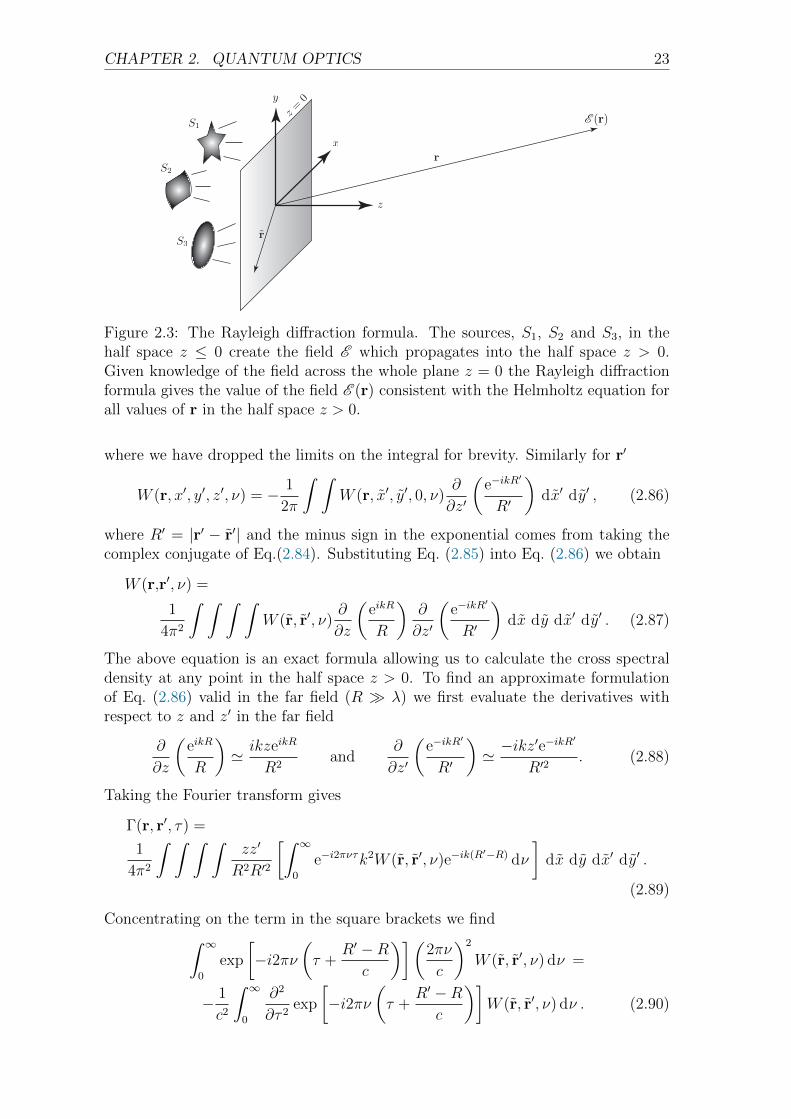
The Rayleigh diffraction formula gives the solution to the Helmholtz equation in thehalf space z > 0 for a field propagating in the positive z direction as a function of thevalues of the field across the entire z = 0 plane, assuming that any sources of the fieldare in the opposing half space z ≤ 0 [Mandel and Wolf, 1995]. Fig.2.3 illustrates thearrangement of the key quantities in the formula. The Rayleigh diffraction formulais
E (x, y, z) = − 1
2π
∫ ∞
−∞
∫ ∞
−∞E (x, y, 0)
∂
∂z
(eikR
R
)dx dy (2.84)
where R2 = (x− x)2 + (y− y)2 + z2, k = 2πν/c and E is a solution to the Helmholtzequation. Since W (r, r′, ν) satisfies the Helmholtz Eqs. (2.82a)(2.82b) we can usethe Rayleigh diffraction formula to find the cross spectral density in the half spacez > 0 assuming we know the values of the cross spectral density in the entire planez = 0. Applying the Rayleigh diffraction formula to the first argument of W (r, r′, ν)i.e. r, and keeping r′ constant, we find
W (x, y, z, r′, ν) = − 1
2π
∫ ∫W (x, y, 0, r′, ν)
∂
∂z
(eikR
R
)dx dy , (2.85)
CHAPTER 2. QUANTUM OPTICS 23
22 2.7. THE RAYLEIGH DIFFRACTION FORMULA
Figure 2.3: The Rayleigh diffraction formula. The sources, S1, S2 and S3, in the halfspace z ≤ 0 create the electric field E which propagates into the half space z > 0.Given knowledge of the field across the whole plane z = 0 the Rayleigh diffractionformula gives the value of the field E(r) consistent with the wave equation for allvalues of r in the half space z > 0.
where k = 2πν/c is the wavenumber. Similarly to the mutual coherence function,the cross spectral density function can also be expressed as an expectation of twocomplex fields [Mandel and Wolf, 1995]
W (r, r′, ν) = 〈E ∗(r, ν)E (r′, ν ′)〉δ(ν − ν ′) (2.83)
where E (r, ν) is a solution to the Helmholtz equation and is the Fourier transformof E(r, t).
2.7 The Rayleigh diffraction formula
E (r) The Rayleigh diffraction formula gives the solution to the Helmholtz equationin the half space z > 0 for a field propagating in the positive z direction as afunction of the values of the field across the entire z = 0 plane, assuming thatany sources of the field are in the opposing half space z ≤ 0 [Mandel and Wolf,1995]. Fig.2.3 illustrates the arrangement of the key quantities in the formula. TheRayleigh diffraction formula is
E (x, y, z) = − 1
2π
∫ ∞
−∞
∫ ∞
−∞E (x, y, 0)
∂
∂z
(eikR
R
)dx dy (2.84)
where R2 = (x− x)2+(y− y)2+ z2, k = 2πν/c and E is a solution to the Helmholtzequation. Since W (r, r′, ν) satisfies the Helmholtz Eqs. (2.82a)(2.82b) we can usethe Rayleigh diffraction formula to find the cross spectral density in the half spacez > 0 assuming we know the values of the cross spectral density in the entire planez = 0. Applying the Rayleigh diffraction formula to the first argument of W (r, r′, ν)i.e. r, and keeping r′ constant, we find
W (x, y, z, r′, ν) = − 1
2π
∫ ∫W (x, y, 0, r′, ν)
∂
∂z
(eikR
R
)dx dy , (2.85)
Figure 2.3: The Rayleigh diffraction formula. The sources, S1, S2 and S3, in thehalf space z ≤ 0 create the field E which propagates into the half space z > 0.Given knowledge of the field across the whole plane z = 0 the Rayleigh diffractionformula gives the value of the field E (r) consistent with the Helmholtz equation forall values of r in the half space z > 0.
where we have dropped the limits on the integral for brevity. Similarly for r′
W (r, x′, y′, z′, ν) = − 1
2π
∫ ∫W (r, x′, y′, 0, ν)
∂
∂z′
(e−ikR
′
R′
)dx′ dy′ , (2.86)
where R′ = |r′ − r′| and the minus sign in the exponential comes from taking thecomplex conjugate of Eq.(2.84). Substituting Eq. (2.85) into Eq. (2.86) we obtain
W (r,r′, ν) =
1
4π2
∫ ∫ ∫ ∫W (r, r′, ν)
∂
∂z
(eikR
R
)∂
∂z′
(e−ikR
′
R′
)dx dy dx′ dy′ . (2.87)
The above equation is an exact formula allowing us to calculate the cross spectraldensity at any point in the half space z > 0. To find an approximate formulationof Eq. (2.86) valid in the far field (R λ) we first evaluate the derivatives withrespect to z and z′ in the far field
∂
∂z
(eikR
R
)' ikzeikR
R2and
∂
∂z′
(e−ikR
′
R′
)' −ikz
′e−ikR′
R′2. (2.88)
Taking the Fourier transform gives
Γ(r, r′, τ) =
1
4π2
∫ ∫ ∫ ∫zz′
R2R′2
[∫ ∞
0
e−i2πντk2W (r, r′, ν)e−ik(R′−R) dν
]dx dy dx′ dy′ .
(2.89)
Concentrating on the term in the square brackets we find∫ ∞
0
exp
[−i2πν
(τ +
R′ −Rc
)](2πν
c
)2
W (r, r′, ν) dν =
− 1
c2
∫ ∞
0
∂2
∂τ 2exp
[−i2πν
(τ +
R′ −Rc
)]W (r, r′, ν) dν . (2.90)
24 2.8. MONOCHROMATIC APPROXIMATION
Exchanging the order of differentiation and integration leads to
− 1
c2
∫ ∞
0
∂2
∂τ 2exp
[−i2πν
(τ +
R′ −Rc
)]W (r, r′, ν) dν =
− 1
c2
∂2
∂τ 2Γ(r, r′, τ + (R′ −R)/c), (2.91)
and we find for the mutual degree of coherence in the far field
Γ(r, r′, τ) = − 1
4π2c2
∫ ∫ ∫ ∫zz′
R2R′2∂2
∂τ 2Γ(r, r′, τ + (R′ −R)/c) dx dy dx′ dy′ .
(2.92)
The integrals over the variables x, y, x′, and y′ all take place over the z = 0 planewhere the mutual degree of coherence is known for all pairs of coordinates.
2.8 Monochromatic approximation
If the fields are monochromatic, or at least approximately so, Eq. (2.92) takes amuch simpler form. Looking back to the term in parenthesis from Eq. (2.89) wemake the approximation
∫ ∞
0
exp
[−i2πν
(τ +
R′ −Rc
)](2πν
c
)2
W (r, r′, ν) dν ≈(
2πν
c
)2 ∫ ∞
0
exp
[−i2πν
(τ +
R′ −Rc
)]W (r, r′, ν) dν (2.93)
where ν is the central frequency of the field. Which leads to the much simplerexpression for Γ(r, r′, τ)
Γ(r, r′, τ) =( νc
)2∫ ∫ ∫ ∫
zz′
R2R′2Γ(r, r′, τ + (R′ −R)/c) dx dy dx′ dy′ (2.94)
where we no longer require the second derivative of Γ with respect to τ . This coversthe basic ideas of coherence and quantum optics that we shall make frequent useof in later chapters. In the next chapter we give an account of estimation theory,which we will again make frequent use of later.
Chapter 3
Estimation Theory
In this section we give an overview of the field of estimation theory, first examiningthe classical theory and then exploring the quantum formalism. The fundamentaltask of estimation theory is to estimate certain values or parameters, from a setof data which exhibit a statistical nature. In the classical theory the statisticalaspects of the data can be regarded as occurring due to any number of experimentaluncertainties whereas in the quantum formalism the statistical behaviour is directlyrelated to the fundamental uncertainty present in a quantum state. A key quantityin estimation theory is the Fisher information. Here we will derive the form ofthe Fisher information and explain it’s relevance to parameter estimation problems.Analogously, in the quantum regime we encounter the quantum Fisher information.Again we derive this quantity and explore its relevance.
3.1 Classical estimation theory
The problem of estimating a set of parameters θ = θ1, . . . , θn from a set of ob-servation data x = x[1], . . . , x[N ] is the object of classical estimation theory. Theequations which govern how the observed data is used to provide a value for theparameters θ are known as estimators. Symbolically we write
θ = f(x), (3.1)
where we use the caron · to denote an estimator. Typically in estimation theorywe use the caret · to denote an estimator, however since this was used in the pre-vious chapter to denote a quantum operator here we will use the caron instead.The distinction between the actual value of the parameters θ and an estimate θ iscrucially important. Whereas the actual value of the parameter θ is a number orset of numbers, the estimate of the parameter is, in general, a random variable orset of random variables. Two sets of observation data may be obtained for whichthe parameters are equal, θ1 = θ2, but, due to the probabilistic nature of the data,the exact values of the observations are not equal x1 6= x2. In general the estimateswill not be equal since they are derived from two different data sets using the sameprocedure.
The example above demonstrates an important feature of estimators. Sincethe values of the parameters are equal, we would like the estimates to be equal.This would correspond to a perfect estimator, one which, given any data set oflength N , returns the exact values of the parameters. This is clearly an unrealistic
25
26 3.1. CLASSICAL ESTIMATION THEORY
idealisation. However, when the above example is performed, we expect that theestimates are at least similar. This leads us to a natural characterisation of theestimators performance, namely the variance of the estimator.
The aim in estimation theory is to identify an estimator with the smallest possiblevariance, therefore leading to estimates that are, on average, as close as they canbe to the actual values θ. In order to achieve this goal, we must know the jointprobability distribution function (PDF) of our data p(x|θ) = p(x[1], . . . , x[N ]|θ),which gives the probability of obtaining all observations x[1], . . . , x[N ] given thevalues of the parameters θ.
3.1.1 The Cramer-Rao bound
In general it is not possible to state exactly what the variance of our estimator is.However, it is usually possible to obtain a lower bound on the variance. Variousmethods for bounding the estimators variance exist, the most commonly used beingthe Cramer-Rao bound.
Consider the single parameter estimation problem, θ = θ. We define the varia-tion in an estimate of θ to be δθ = θ−〈θ〉, where 〈θ〉 is the expectation value of theestimator defined by
〈θ〉 =
∫dx p(x|θ)θ. (3.2)
We purposefully avoid the notation ∆θ which should be reserved for the error ∆θ =θ − θ. The variance of the estimator should not be confused with the mean squareerror, which is defined by
〈(∆θ)2〉 = 〈(θ − θ)2〉 = 〈θ2〉 − 2〈θ〉θ + θ2 = 〈θ2〉 − 〈θ〉2 + 〈θ〉2 − 2〈θ〉θ + θ2
= Var(θ) + B(θ)2, (3.3)
where B(θ) is the bias of the estimator defined as B(θ) = 〈θ〉 − θ and we havedefined the variance of the estimator to be Var(θ) = 〈θ2〉 − 〈θ〉2. We see directlyfrom Eq. (3.3) that the mean square error is equal to the variance if and only if thethe bias is 0. We refer to such an estimator as unbiased, for which the equation〈θ〉 = θ holds.
Now, since
∫dx p(x|θ)〈θ〉 = 〈θ〉, (3.4)
we find
〈δθ〉 =
∫dx p(x|θ)(θ − 〈θ〉) = 0. (3.5)
For M independent measurements with outcomes x1, . . . ,xM we can write
∫dx1 . . .
∫dxM p(x1|θ) . . . p(xM |θ)δθ = 0. (3.6)
CHAPTER 3. ESTIMATION THEORY 27
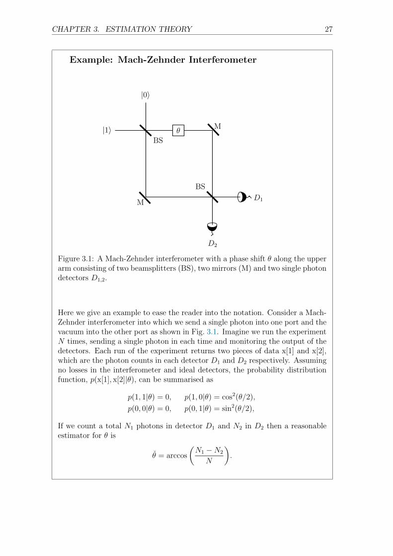
Example: Mach-Zehnder Interferometer
BS
MD1
D2
|1〉
|0〉
BS
Mθ
Figure 3.1: A Mach-Zehnder interferometer with a phase shift θ along the upperarm consisting of two beamsplitters (BS), two mirrors (M) and two single photondetectors D1,2.
Here we give an example to ease the reader into the notation. Consider a Mach-Zehnder interferometer into which we send a single photon into one port and thevacuum into the other port as shown in Fig. 3.1. Imagine we run the experimentN times, sending a single photon in each time and monitoring the output of thedetectors. Each run of the experiment returns two pieces of data x[1] and x[2],which are the photon counts in each detector D1 and D2 respectively. Assumingno losses in the interferometer and ideal detectors, the probability distributionfunction, p(x[1], x[2]|θ), can be summarised as
p(1, 1|θ) = 0, p(1, 0|θ) = cos2(θ/2),
p(0, 0|θ) = 0, p(0, 1|θ) = sin2(θ/2),
If we count a total N1 photons in detector D1 and N2 in D2 then a reasonableestimator for θ is
θ = arccos
(N1 −N2
N
).
28 3.1. CLASSICAL ESTIMATION THEORY
Taking the derivative with respect to θ yields
∫dx1 . . .
∫dxM
M∏
j=1
p(xj|θ)(
M∑
i=1
1
p(xi|θ)∂p(xi|θ)∂θ
δθ +∂δθ
∂θ
)= 0. (3.7)
Since θ = f(x) is an estimator, it does not depend on θ, therefore
∂δθ
∂θ= −∂〈θ〉
∂θ, (3.8)
and
∫dx1 . . .
∫dxM
M∏
j=1
p(xj|θ)∂δθ
∂θ= −
⟨∂〈θ〉∂θ
⟩
= −∂〈θ〉∂θ
, (3.9)
where the last equality holds because ∂θ〈θ〉 is independent of x1, . . . ,xM . We nowuse the Cauchy-Schwarz inequality
|〈x, y〉|2 ≤ 〈x, x〉〈y, y〉, (3.10)
making the substitutions
x =M∑
i=1
1
p(xi|θ)∂p(xi|θ)∂θ
,
y = δθ,
we find
∫dx1 . . .
∫dxM
M∏
j=1
p(xj|θ)(
M∑
i=1
1
p(xi|θ)∂p(xi|θ)∂θ
)2
×∫
dx1 . . .
∫dxM
M∏
j=1
p(xj|θ)(δθ)2 ≥∣∣∣∣∂〈θ〉∂θ
∣∣∣∣2
, (3.11)
where the right hand side is obtained by noticing that 〈x, y〉 = −〈∂θx〉 and −〈∂θx〉 =∂θ〈θ〉, which come directly from Eq. (3.7) and Eq. (3.9) respectively.
We can simplify the first term by noticing that
∫dx1 . . .
∫dxM
M∏
j=1
p(xj|θ)(
M∑
i=1
1
p(xi|θ)∂p(xi|θ)∂θ
)(M∑
k=1
1
p(xk|θ)∂p(xk|θ)
∂θ
)=
M∑
i,k=1
∫dx1 . . .
∫dxM
M∏
j=1
p(xj|θ)p(xi|θ)p(xk|θ)
∂p(xi|θ)∂θ
∂p(xk|θ)∂θ
, (3.12)
CHAPTER 3. ESTIMATION THEORY 29
which for i 6= k gives
∫dxi
∫dxk
∂p(xi|θ)∂θ
∂p(xk|θ)∂θ
=
∫dxi
∂p(xi|θ)∂θ
∫dxk
∂p(xk|θ)∂θ
=∂
∂θ
[ ∫dxi p(xi|θ)
]∂
∂θ
[ ∫dxk p(xk|θ)
]
=
(∂
∂θ1
)2
= 0. (3.13)
Eq. (3.11) now simplifies to
M
∫dx
1
p(x|θ)
(∂p(x|θ)∂θ
)2
〈(δθ)2〉 ≥∣∣∣∣∂〈θ〉∂θ
∣∣∣∣2
. (3.14)
The integral in the previous expression plays a particularly important role in esti-mation theory. It is referred to as the Fisher information and it can be expressed asthe expectation value of the derivative of the log likelihood, ln[p(x|θ)],
I(θ) =
∫dx
1
p(x|θ)
(∂p(x|θ)∂θ
)2
=
∫dx p(x|θ)
(∂ ln[p(x|θ)]
∂θ
)2
=
⟨(∂ ln[p(x|θ)]
∂θ
)2⟩. (3.15)
Physically, the Fisher information represents the average amount of informationabout the parameter θ that we can access through a measurement for which theoutcome probability distribution is p(x|θ). From the definition Eq. (3.15) we see thatthe Fisher information is always positive and from Eq. (3.14) the factor M impliesthat the Fisher information is additive for independent measurements. These areboth important properties for any physical measure of information. Re-arrangingEq. (3.14) and writing the variance as Var(θ) leads directly to the Cramer-Raobound
Var(θ) ≥∣∣∂〈θ〉∂θ
∣∣2
MI(θ), (3.16)
where |∂θ〈θ〉|2 accounts for a possible difference in units between θ and θ. Thisexpression proves that the variance of the estimator θ is bounded from below by theFisher information.
3.1.2 The multi-parameter Cramer-Rao bound
The Cramer-Rao bound as derived in the previous section provides a lower bound forthe variance of a single parameter estimator. We will now derive the multi-parameterCramer-Rao bound that provides a lower bound not only on the variances of theestimators but also on the covariances of the estimators. Starting again from
∫dx1 . . .
∫dxM p(x1|θ) . . . p(xM |θ)δθi = 0, (3.17)
30 3.1. CLASSICAL ESTIMATION THEORY
where δθi = θi − 〈θi〉, we now take the derivative with respect to the parameter θj.This gives
∫dx1 . . .
∫dxM
M∏
k=1
p(xk|θ)
(M∑
l=1
∂ ln[p(xl|θ)]
∂θj
)δθi = −∂〈θi〉
∂θj. (3.18)
For n parameters Eq. (3.18) defines n× n equations, writing
θ =
θ1...θn
, (3.19)
we can write these in vectorial form
∫dx1 . . .
∫dxM
M∏
k=1
p(xk|θ)
(M∑
l=1
∂ ln[p(xl|θ)]
∂θ
)δθT = −∂〈θ〉
∂θ. (3.20)
Multiplying from the left by aT and from the right by b, where a and b are arbi-trary n vectors, allows us to again use the Cauchy-Schwarz inequality. Making thesubstitutions
x =M∑
l=1
aT · ∂ ln[p(xl|θ)]
∂θ,
y = (δθ)T · b,
gives
aT ·∫
dx1 . . .
∫dxM
M∏
k=1
p(xk|θ)
(M∑
l=1
∂ ln[p(xl|θ)]
∂θ
)(M∑
l′=1
∂ ln[p(xl′|θ)]
∂θ
)T
· a
× bT ·∫
dx1 . . .
∫dxM
M∏
k′=1
p(xk′|θ)(δθ)(δθ)T · b ≥∣∣∣∣aT · ∂〈θ〉
∂θ· b∣∣∣∣2
. (3.21)
As in the case for a single parameter, we find that the first term evaluates to 0 unlessl = l′.
Defining the Fisher information matrix as
I(θ) =
∫dx p(x|θ)
(∂ ln[p(x|θ)]
∂θ
)(∂ ln[p(x|θ)]
∂θ
)T
, (3.22)
with elements
[I(θ)]ij =
∫dx p(x|θ)
(∂ ln[p(x|θ)]
∂θi
)(∂ ln[p(x|θ)]
∂θj
), (3.23)
the inequality in Eq. (3.21) now simplifies to
MaT · I(θ) · abT · 〈(δθ)(δθ)T〉 · b ≥∣∣∣∣aT · ∂〈θ〉
∂θ· b∣∣∣∣2
. (3.24)
CHAPTER 3. ESTIMATION THEORY 31
Assuming that the Fisher information matrix can be inverted and since a is arbitrary,we make the assumption
a = [I(θ)−1]T∂〈θ〉∂θ· b, (3.25)
which leads to
MbT ·[∂〈θ〉∂θ
]T
I(θ)−1I(θ)[I(θ)−1]T∂〈θ〉∂θ· bbT · 〈(δθ)(δθ)T〉 · b ≥
∣∣∣∣bT ·[∂〈θ〉∂θ
]T
I(θ)−1∂〈θ〉∂θ· b∣∣∣∣2
. (3.26)
From the definition (3.22) we see that the Fisher information matrix is symmetric,therefore IT = I and
I(θ)[I(θ)−1]T = I(θ)T[I(θ)−1]T = [I(θ)−1I(θ)]T = 1. (3.27)
The Fisher information matrix is positive definite and therefore so is its inverse. Fora set of real parameters the term in the absolute value is real and we find
MbT · 〈(δθ)(δθ)T〉 · b ≥ bT ·[∂〈θ〉∂θ
]T
I(θ)−1∂〈θ〉∂θ· b. (3.28)
Remembering that b is arbitrary we have
〈(δθ)(δθ)T〉 ≥ 1
M
[∂〈θ〉∂θ
]T
I(θ)−1∂〈θ〉∂θ
. (3.29)
The term 〈(δθ)(δθ)T〉 is the covariance matrix between our estimators θ1, . . . , θn,whose elements are bounded by
Cov(θi, θj) ≥1
M
(∂〈θj〉∂θi
∂〈θi〉∂θj
)[I(θ)−1]ij. (3.30)
This is the Cramer-Rao bound for multiple parameters and reduces to Eq. (3.16)when n = 1.
3.1.3 Estimating parameters
As previously mentioned, the Cramer-Rao bound places a lower bound on the vari-ance of an estimator. In order to achieve the Cramer-Rao bound a suitable estimatormust be chosen. Numerous methods for choosing an estimator exist and in order toensure that we obtain an estimator that performs well, we must ensure that the rightmethod is applied. Unfortunately there is no single method for choosing an estima-tor that applies to all situations and we must make a decision of which method touse based on our understanding of the situation. In general the Cramer-Rao boundis dependent on the parameters θ. Any estimator that achieves the Cramer-Raobound for all values of θ is called an efficient estimator.
We first consider the procedure of maximum likelihood estimation which, due toits simplicity is used in numerous applications. The maximum likelihood procedure

32 3.2. QUANTUM ESTIMATION THEORY
attempts to find the values of the parameters θ that maximise the log likelihoodfunction ln[p(x|θ)]. In some circumstances this may be as simple as taking thederivative of the likelihood function and equating it to zero to find the maximum.However, this is not always a straightforward operation and alternative methods forobtaining the maximum likelihood estimator must be used.
The maximum likelihood estimator may also be obtained numerically via aniterative algorithm. The scoring algorithm is one such procedure which proceedsaccording to the iterative equation [Kay, 1993]
I(θ(k))θ(k+1) = I(θ(k))θ(k) +∂ ln[p(x|θ)]
∂θ
∣∣∣∣θ=θ(k)
, (3.31)
where θ(k) is the kth iteration of the estimator θ, X(θ)|θ=θ(k) denotes evaluation ofX at the point θ = θ(k) and I(θ) is the Fisher information. This method takes aninitial guess of the parameter, θ(0) and via successive iterations gradually hones inon the actual values of parameters θ. When evaluating the Cramer-Rao bound, ifwe calculate the Fisher information via Eq. (3.22) then the term ∂θ ln[p(x|θ)] hasalready been determined and the scoring algorithm proceeds without difficulty.
3.2 Quantum estimation theory
In the previous section we demonstrated how the variance of an unbiased estimatorcan be bounded from below by the Fisher information via the Cramer-Rao bound.The probabilistic nature of the data we measure only allows us to make statisticalinferences about any parameters on which the data depend. At this stage a naturalquestion arises: what happens when the probabilistic nature of the data is a directconsequence of quantum uncertainty as opposed to specific detection uncertainties?In this section we show that the quantum Fisher information, IQ, provides a nat-ural generalisation to the Fisher information of the previous section, which shallhenceforth be referred to as the classical Fisher information or just I.
3.2.1 The quantum Fisher information
Although not the first researchers to define the quantum Fisher information, Braun-stein and Caves demonstrated that the quantum Fisher information can be consid-ered as the solution to two distinct optimization problems [Braunstein and Caves,1994]. By considering the discrimination of neighbouring quantum states as a pa-rameter estimation problem where the parameter we wish to measure, θ, definesa path through the state space of the system, they showed that the optimal per-formance of any estimator for θ is given by the quantum Fisher information. Thequantum Fisher information is therefore independent of the measurement procedurechosen and is in fact only a function of the state itself. It therefore provides a lowerbound which is dictated by the geometry of state space for the system and thereforecannot be overcome without modifying the state itself. In some cases, modificationof the state is not an issue and we can seek to find the best state to optimise mea-surements of θ, however in some circumstances this is not possible and the best wecan do is seek a measurement with achieves the minimum variance via the quantumCramer-Rao bound.
CHAPTER 3. ESTIMATION THEORY 33
We start with the single parameter version of the classical Fisher information asgiven by Eq. (3.15) only now we use the Born rule to find the probability distributionp(x|θ)
p(x|θ) = Tr[ρ(θ)Ex
], (3.32)
where ρ(θ) is the state which depends on the parameter θ that we want to estimateand Ex is the POVM element describing the measurement which produces outcomex. A detailed account of the use of POVMs is given in section 4.1. To calculate theFisher information we need to take the derivative of this probability distributionwith respect to the parameter θ. Taking the derivative of Eq. (3.32) gives
∂
∂θp(x|θ) = Tr
[∂
∂θρEx
]≡ Tr
[∂θρEx
], (3.33)
where we have dropped the ρ dependence on θ and henceforth this shall be assumed.We now introduce the symmetric logarithmic derivative super-operator (SLD) im-plicitly defined by the equation
ρ′ =Lρ(ρ
′)ρ+ ρLρ(ρ′)
2, (3.34)
where Lρ(ρ′) is the symmetric logarithmic derivative and we have defined ρ′ = ∂θρ.
Eq. (3.34) takes the form of a Lyapunov equation, for which the solution is [Paris,2009]
Lρ(ρ′) = 2
∫ ∞
0
dt e−ρtρ′e−ρt. (3.35)
In the basis that diagonalises ρ we find
Lρ(ρ′) = 2
∑
i,j
ρ′ijpi + pj
|i〉〈j|, (3.36)
where pi and pj are the eigenvalues of ρ and the sum is taken over all i, j that satisfypi,j 6= 0.
Using the fact that ρ is Hermitian, and therefore pi,j are real, we see that thesymmetric logarithmic derivative is also Hermitian
L †ρ (ρ′) = 2
∑
i,j
(ρ′ij)∗
pi + pj|j〉〈i| = 2
∑
i,j
ρ′jipi + pj
|j〉〈i| = Lρ(ρ′). (3.37)
Inserting the form of the derivative given by the SLD, Eq. (3.34), into Eq. (3.33)gives us
∂θp(x|θ) =1
2Tr[ρExLρ(ρ
′)]
+1
2Tr[ρLρ(ρ
′)Ex], (3.38)
34 3.2. QUANTUM ESTIMATION THEORY
and using the property, Tr[ABC] = (Tr[ACB])∗ for Hermitian A, B and C 1, wefind
∂θp(x|θ) = Re
Tr[ρExLρ(ρ
′)]
. (3.39)
From the definition of the Fisher information Eq. (3.15) and the expressions justobtained, we find that the classical Fisher information for a measurement of theoperator Ex on the state ρ
I =
∫dx
ReTr[ρExLρ(ρ′)]2
Tr[ρEx]. (3.40)
We now want to maximise the classical Fisher information over all possible mea-surements Ex. To do this we first find a measurement-independent upper boundfor I and then show that this upper bound is achievable for an appropriate choiceof Ex. We therefore will conclude that the Fisher information found is an intrinsicproperty of the state ρ meaning that it provides a lower bound for the variance of anestimator for θ (via the Cramer-Rao bound) which a change of Ex cannot overcome.
To find the measurement independent form of I we first make use of the fact thatfor complex α, Reα2 ≤ |α|2, where equality implies that α is real. This allows usto express the Fisher information in Eq. (3.40) as
I ≤∫
dx|Tr[ρExLρ(ρ
′)]|2Tr[ρEx]
=
∫dx
∣∣∣∣Tr[ρExLρ(ρ
′)]
Tr[ρEx]12
∣∣∣∣2
, (3.41)
where equality holds iff ImTr[ρExLρ(ρ′)] = 0. Now, from the Cauchy-Schwarz
inequality we find
∫dx
∣∣∣∣Tr[ρExLρ(ρ
′)]
Tr[ρEx]12
∣∣∣∣2
=
∫dx
∣∣∣∣Tr[ρ
12 E
12x E
12x Lρ(ρ
′)ρ12 ]
Tr[ρEx]12
∣∣∣∣2
=
∫dx
∣∣∣∣∣Tr
[ρ
12 E
12x
Tr[ρEx]12
E12x Lρ(ρ
′)ρ12
]∣∣∣∣∣
2
≤∫
dxTr[E
12x Lρ(ρ
′)ρ12 (E
12x Lρ(ρ
′)ρ12 )†]
(3.42a)
=
∫dxTr
[ρLρ(ρ
′)ExLρ(ρ′)]
= Tr[ρL 2
ρ (ρ′)]. (3.42b)
1To prove this assertion we start from right hand side and work back. First we write the lefthand side in index notation
(Tr[ACB])∗ =∑
i,j,k
(AijCjkBki)∗ =
∑
i,j,k
A∗ijC∗jkB
∗ki.
Now using the fact the A, B, and C are Hermitian we find
(Tr[ACB])∗ =∑
i,j,k
AjiCkjBik =∑
i,j,k
AjiBikCkj = Tr[ABC],
and we see that (Tr[ACB])∗ = Tr[ABC] as we set out to prove.
CHAPTER 3. ESTIMATION THEORY 35
In order to obtain equality in Eq. (3.42a) requires that the equation
E12x ρ
12
Tr[ρEx]=
E12x Lρ(ρ
′)ρ12
Tr[ρExLρ(ρ′)], (3.43)
is satisfied for all values of θ [Paris, 2009]. This is achieved when the operator Exis a one dimensional projector that projects onto a complete set of eigenstates ofLρ(ρ
′) [Braunstein et al., 1996].The upper bound for I is therefore an achievable. The quantum Fisher informa-
tion is therefore given by
IQ = Tr[ρL 2
ρ (ρ′)], (3.44)
or by substituting from Eq. (3.34) into Eq. (3.42b)
Tr[ρL 2
ρ (ρ′)]
= 2Tr[ρ′Lρ(ρ′)]− Tr
[ρL 2
ρ (ρ′)]
=⇒ IQ = Tr[ρ′Lρ(ρ′)]. (3.45)
We can now lower bound the variance of any estimator of θ by the quantum Cramer-Rao bound
Var(θ) ≥∂〈θ〉∂θ
MIQ, (3.46)
which is achievable for a measurement satisfying the conditions given above.As pointed out by various authors [Braunstein and Caves, 1994,Braunstein et al.,
1996, Paris, 2009], the quantum Fisher information adheres to a geometrical inter-pretation. The quantum Fisher information is proportional to the Bures metric,which is used to calculate distances in the state space of mixed quantum systems.When viewed as a metric the quantum Fisher information tells us how quickly aninfinitesimal change of the parameter moves the family of states parameterised by θthrough the space. A large quantum Fisher information implies that small changesof the parameter can move the state to a new state far apart from the initial one.The further apart these states live in the state space the more distinguishable theyare and therefore the easier it is to tell them apart in an experiment. If small changesin the parameter can easily be determined then the parameter can be measured withhigh precision, this is the basis of the quantum Cramer-Rao bound.
3.2.2 The multi-parameter quantum Cramer-Rao bound
Just as in the classical treatment, the quantum theory of parameter estimation canalso be extended to the problem of estimating multiple parameters simultaneously.Again writing the n parameters to be estimated as θ = (θ1, . . . , θn)T we find thatthe bound for the covariance matrix of our estimators is
Cov(θi, θj) ≥1
M
(∂〈θj〉∂θi
∂〈θi〉∂θj
)[I−1
Q ]ij, (3.47)
where the elements of the quantum Fisher information matrix are given by
[IQ]ij = Tr[ρ(LiLj + LjLi)], (3.48)

36 3.2. QUANTUM ESTIMATION THEORY
and the SLD for the parameter θi is defined via the equation
∂ρ
∂θi=
Liρ+ ρLi
2. (3.49)
The subscript and argument have been dropped from L for brevity. Using thedefinition Eq. (3.49) in Eq. (3.48) we find
[IQ]ij = Tr[(∂iρ)Lj], (3.50)
where ∂iρ ≡ ∂∂θiρ.
In general the non-commutativity of quantum mechanics renders this boundunachievable except when [Monras and Illuminati, 2011]
Tr[ρ[Li,Lj]] = 0. (3.51)
Finding the SLD for a set of parameters therefore allows us to determine if we canperform a joint efficient estimation and, from the previous section, allows us to findthe optimal estimator. For these reasons determining the SLD is of paramountimportance for a general quantum parameter estimation problem.
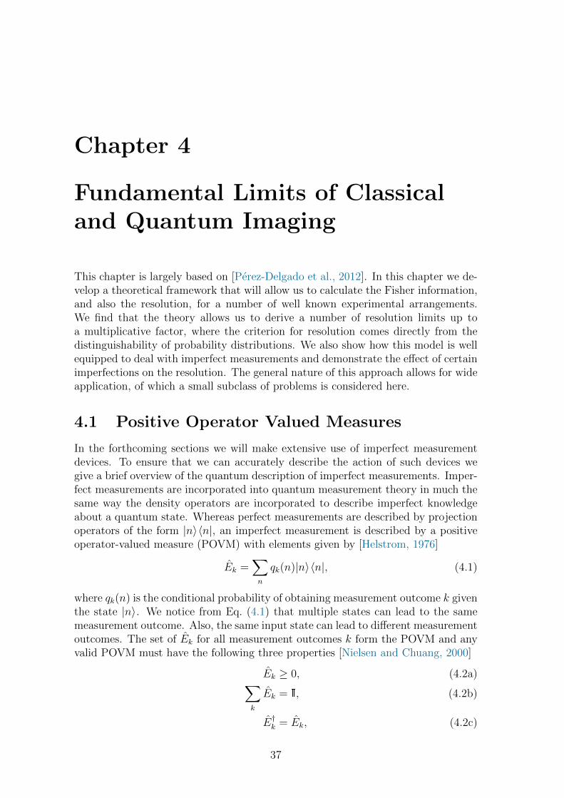
Chapter 4
Fundamental Limits of Classicaland Quantum Imaging
This chapter is largely based on [Perez-Delgado et al., 2012]. In this chapter we de-velop a theoretical framework that will allow us to calculate the Fisher information,and also the resolution, for a number of well known experimental arrangements.We find that the theory allows us to derive a number of resolution limits up toa multiplicative factor, where the criterion for resolution comes directly from thedistinguishability of probability distributions. We also show how this model is wellequipped to deal with imperfect measurements and demonstrate the effect of certainimperfections on the resolution. The general nature of this approach allows for wideapplication, of which a small subclass of problems is considered here.
4.1 Positive Operator Valued Measures
In the forthcoming sections we will make extensive use of imperfect measurementdevices. To ensure that we can accurately describe the action of such devices wegive a brief overview of the quantum description of imperfect measurements. Imper-fect measurements are incorporated into quantum measurement theory in much thesame way the density operators are incorporated to describe imperfect knowledgeabout a quantum state. Whereas perfect measurements are described by projectionoperators of the form |n〉〈n|, an imperfect measurement is described by a positiveoperator-valued measure (POVM) with elements given by [Helstrom, 1976]
Ek =∑
n
qk(n)|n〉〈n|, (4.1)
where qk(n) is the conditional probability of obtaining measurement outcome k giventhe state |n〉. We notice from Eq. (4.1) that multiple states can lead to the samemeasurement outcome. Also, the same input state can lead to different measurementoutcomes. The set of Ek for all measurement outcomes k form the POVM and anyvalid POVM must have the following three properties [Nielsen and Chuang, 2000]
Ek ≥ 0, (4.2a)∑
k
Ek = I, (4.2b)
E†k = Ek, (4.2c)
37
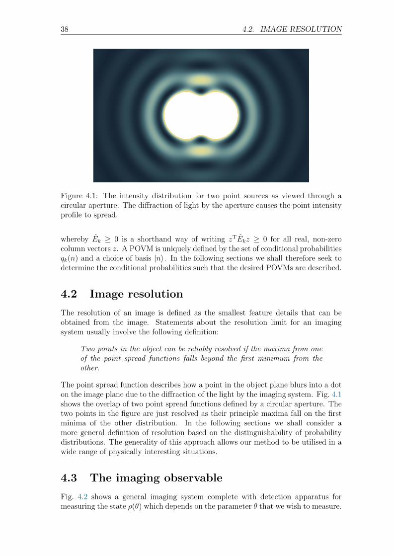
38 4.2. IMAGE RESOLUTION
Figure 4.1: The intensity distribution for two point sources as viewed through acircular aperture. The diffraction of light by the aperture causes the point intensityprofile to spread.
whereby Ek ≥ 0 is a shorthand way of writing zTEkz ≥ 0 for all real, non-zerocolumn vectors z. A POVM is uniquely defined by the set of conditional probabilitiesqk(n) and a choice of basis |n〉. In the following sections we shall therefore seek todetermine the conditional probabilities such that the desired POVMs are described.
4.2 Image resolution
The resolution of an image is defined as the smallest feature details that can beobtained from the image. Statements about the resolution limit for an imagingsystem usually involve the following definition:
Two points in the object can be reliably resolved if the maxima from oneof the point spread functions falls beyond the first minimum from theother.
The point spread function describes how a point in the object plane blurs into a doton the image plane due to the diffraction of the light by the imaging system. Fig. 4.1shows the overlap of two point spread functions defined by a circular aperture. Thetwo points in the figure are just resolved as their principle maxima fall on the firstminima of the other distribution. In the following sections we shall consider amore general definition of resolution based on the distinguishability of probabilitydistributions. The generality of this approach allows our method to be utilised in awide range of physically interesting situations.
4.3 The imaging observable
Fig. 4.2 shows a general imaging system complete with detection apparatus formeasuring the state ρ(θ) which depends on the parameter θ that we wish to measure.

CHAPTER 4. FUNDAMENTAL LIMITS 39
O
L
ρ(θ)
Sx
Figure 4.2: General imaging system. Light from the object O is manipulated bysome optical system L and is then incident on the substrate S. The substratemakes a measurement (possibly imperfect) of the state ρ(θ) which depends uponthe parameter we wish to measure θ.
We consider the detector, S, to be granular, consisting of N pixels of length ` makingthe total length of the substrate L = N`. The pixels are distinguished by theirposition x on the substrate. We denote the image intensity by ik and the probabilityof measuring ik at position x is given by pk(x). The average intensity recorded atposition x is given by I(x) =
∑k ikpk(x). We can calculate the probabilities pk(x)
from the Born rule pk(x) = Tr[ρ(θ)Ek(x)] where Ek(x) is the measurement operatorassociated with the outcome ik. The set of operators Ek(x) form a positive operator-valued measure (POVM) for each pixel,
∑k Ek(x) = I(x).
The image I(x) need not be restricted to the expectation value of the intensityat pixel x. In principle any observable quantity can be identified as the “image”,for example we may choose as our observable the equal-time, nth order intensitycorrelation function G(n)(x1, . . . ,xn) [Oppel et al., 2012]. Using the Born rule andthe definition of the image we find
I(x) =∑
k
ikTr[ρ(θ)Ek(x)
]= Tr
[∑
k
ikρ(θ)Ek(x)
]≡ Tr
[ρ(θ)I(x)
], (4.3)
where we have defined the imaging operator to be I(x) =∑
k ikEk(x). In thesimplest case, the imaging operator simply records the intensity at the position x,which is directly proportional to the photon number k. The POVM for such asubstrate is simply given by Ek(x) = |k〉x〈k| and ik = k. Later we will make useof more complicated POVM’s when we wish to consider the effects of imperfectmeasurements.
Typically, measurements in imaging can be described by operators that are di-agonal in the Fock basis since they usually consist of photon counts at each pixel.
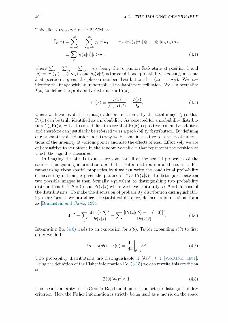
40 4.3. THE IMAGING OBSERVABLE
This allows us to write the POVM as
Ek(x) =∞∑
n1=0
· · ·∞∑
nN=0
qk(x|n1, . . . , nN)|n1〉1〈n1| ⊗ · · · ⊗ |nN〉N 〈nN |
≡∑
~n
qk(x|~n)|~n〉〈~n|, (4.4)
where∑
~n =∑
n1· · ·∑nN
, |ni〉i being the ni photon Fock state at position i, and|~n〉 = |n1〉1⊗· · ·⊗|nN〉N and qk(x|~n) is the conditional probability of getting outcomek at position x given the photon number distribution ~n = (n1, . . . , nN). We nowidentify the image with an unnormalised probability distribution. We can normaliseI(x) to define the probability distribution Pr(x)
Pr(x) ≡ I(x)∑x′ I(x′)
=I(x)
I0
, (4.5)
where we have divided the image value at position x by the total image I0 so thatPr(x) can be truly identified as a probability. As expected for a probability distribu-tion
∑x Pr(x) = 1. It is not difficult to see that Pr(x) is positive real and σ-additive
and therefore can justifiably be referred to as a probability distribution. By definingour probability distribution in this way we become insensitive to statistical fluctua-tions of the intensity at various points and also the effects of loss. Effectively we areonly sensitive to variations in the random variable x that represents the position atwhich the signal is measured
In imaging the aim is to measure some or all of the spatial properties of thesource, thus gaining information about the spatial distribution of the source. Pa-rameterising these spatial properties by θ we can write the conditional probabilityof measuring outcome x given the parameter θ as Pr(x|θ). To distinguish betweentwo possible images is then formally equivalent to distinguishing two probabilitydistributions Pr(x|θ = 0) and Pr(x|θ) where we have arbitrarily set θ = 0 for one ofthe distributions. To make the discussion of probability distribution distinguishabil-ity more formal, we introduce the statistical distance, defined in infinitesimal formas [Braunstein and Caves, 1994]
ds 2 =∑
x
dPr(x|θ) 2
Pr(x|θ) =∑
x
[Pr(x|dθ)− Pr(x|0)]2
Pr(x|θ) . (4.6)
Integrating Eq. (4.6) leads to an expression for s(θ), Taylor expanding s(θ) to firstorder we find
δs ≡ s(δθ)− s(0) =ds
dθ
∣∣∣∣θ=0
δθ. (4.7)
Two probability distributions are distinguishable if (δs)2 ≥ 1 [Wootters, 1981].Using the definition of the Fisher information Eq. (3.15) we can rewrite this conditionas
I(0)(δθ)2 ≥ 1. (4.8)
This bears similarity to the Cramer-Rao bound but it is in fact our distinguishabilitycriterion. Here the Fisher information is strictly being used as a metric on the space

CHAPTER 4. FUNDAMENTAL LIMITS 41
of probabilities that are defined by Eq. (4.5) and as such should not be confusedwith the Fisher information associated with a measurement of the intensity along thesubstrate. Whilst we would expect the Fisher information for such a measurementto depend on the noise, the quantity I defined here is independent of such noisedue to the normalisation in Eq. (4.5). Using the probability distribution given inEq. (4.5) to calculate the Fisher information leads to
I(θ) =∑
x
I0
〈I(x)〉
[1
I0
∂〈I(x)〉∂θ
− 〈I(x)〉I2
0
∂I0
∂θ
]2
=∑
x
[1
〈I(x)〉I0
(∂〈I(x)〉∂θ
)2
− 2
I20
∂I0
∂θ
∂〈I(x)〉∂θ
+〈I(x)〉I3
0
(∂I0
∂θ
)2]
=∑
x
1
〈I(x)〉I0
(∂〈I(x)〉∂θ
)2
− 1
I20
(∂I0
∂θ
)2
, (4.9)
where we have used
∑
x
∂〈I(x)〉∂θ
=∂
∂θ
∑
x
〈I(x)〉 =∂I0
∂θ. (4.10)
Now we have an expression for the Fisher information in terms of the image 〈I(x)〉and the first derivative of the image with respect to θ, which we can use along withEq. (4.8) to determine the statistical resolution.
4.4 Examples
We now use the theory outlined above to show that the results are consistent withwell known resolution limits. First we consider the double slit experiment, in whichthe image is the interference pattern in the far field
〈I(x)〉 = cos2
(kθx
2R
), (4.11)
where k is the wavenumber of the radiation used and R is the distance from the slitto the image plane. Taking the limit of a continuous detection medium, we find theprobability distribution Pr(x|θ) to be
Pr(x|θ) =kθ cos2
(kθx2R
)
kθA+ sin(kθA)(4.12)
where A = xmax/R is the numerical aperture of the system [Lipson et al., 2011].From this we derive the Fisher information
I(θ) =1
θ2− 2A3θk3
3[Aθk + sin(Aθk)]+A2k2 [A2θ2k2 − 2 cos(Aθk)− 2]
[Aθk + sin(Aθk)]2. (4.13)
In order to resolve the two slits the distance θ between them must be greater thanthe uncertainty δθ. We therefore find that the two slits can be resolved if I(θ)θ2 ≥ 1.Multiplying Eq. (4.13) by θ2 and making the substitution z = kθA we find
I(θ)θ2 = 1− 2z3
3(z + sin z)+z2(z2 − 2 cos z − 2)
(z + sin z)2. (4.14)
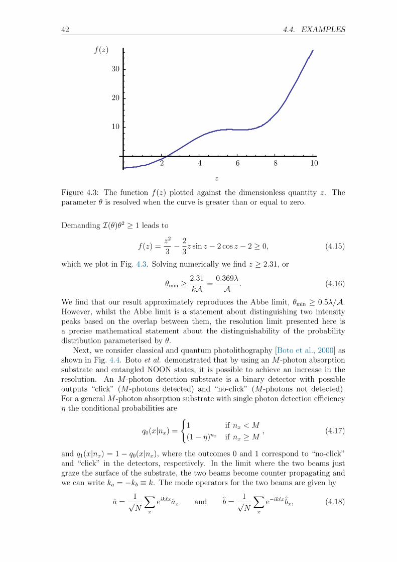
42 4.4. EXAMPLES
2 4 6 8 10
10
20
30
f(z)
z
Figure 4.3: The function f(z) plotted against the dimensionless quantity z. Theparameter θ is resolved when the curve is greater than or equal to zero.
Demanding I(θ)θ2 ≥ 1 leads to
f(z) =z2
3− 2
3z sin z − 2 cos z − 2 ≥ 0, (4.15)
which we plot in Fig. 4.3. Solving numerically we find z ≥ 2.31, or
θmin ≥2.31
kA =0.369λ
A . (4.16)
We find that our result approximately reproduces the Abbe limit, θmin ≥ 0.5λ/A.However, whilst the Abbe limit is a statement about distinguishing two intensitypeaks based on the overlap between them, the resolution limit presented here isa precise mathematical statement about the distinguishability of the probabilitydistribution parameterised by θ.
Next, we consider classical and quantum photolithography [Boto et al., 2000] asshown in Fig. 4.4. Boto et al. demonstrated that by using an M -photon absorptionsubstrate and entangled NOON states, it is possible to achieve an increase in theresolution. An M -photon detection substrate is a binary detector with possibleoutputs “click” (M -photons detected) and “no-click” (M -photons not detected).For a general M -photon absorption substrate with single photon detection efficiencyη the conditional probabilities are
q0(x|nx) =
1 if nx < M
(1− η)nx if nx ≥M, (4.17)
and q1(x|nx) = 1 − q0(x|nx), where the outcomes 0 and 1 correspond to “no-click”and “click” in the detectors, respectively. In the limit where the two beams justgraze the surface of the substrate, the two beams become counter propagating andwe can write ka = −kb ≡ k. The mode operators for the two beams are given by
a =1√N
∑
x
eik`xax and b =1√N
∑
x
e−ik`xbx, (4.18)

CHAPTER 4. FUNDAMENTAL LIMITS 43
which we write in terms of the spatially localised modes ax and bx, N being thenumber of pixels.
The mode operator at position x on the substrate is
ex =ax + bx√
2. (4.19)
For classical, single photon lithography the POVM elements E0(x) and E1(x) are
E0(x) =∞∑
nx=0
(1− η)nx|nx〉x〈nx| and E1(x) =∞∑
nx=0
[1− (1− η)nx ]|nx〉x〈nx|,
(4.20)
where |nx〉x are the Fock basis for the mode ex, i.e. ex|nx〉x =√nx|nx − 1〉x.
a be
substrate
Figure 4.4: Photolithography. The two nearly counter propagating beams a andb interfere producing a pattern on the substrate. The phase shift θ translates theimage along the substrate.
To simplify the notation slightly we will drop the x subscript on the bras andkets. Defining the measurement outcomes to be i0 = 0 and i1 = 1 without lossof generality, we find the image is
〈I(x)〉 =∞∑
nx=0
[1− (1− η)nx ]〈nx|ρ|nx〉, (4.21)
where the term 〈nx|ρ|nx〉, becomes |〈nx|ψ〉|2 for pure states.In the classical case the input state is the single photon state
|ψ〉 =|1, 0〉ab + eiθ|0, 1〉ab√
2. (4.22)
It might at first seem strange to identify the highly path entangled state |ψ〉 with aclassical state, however we note that in the canonical example of a classical state, thecoherent state, all the photons are completely statistically independent. Thereforethe action of a beamsplitter on a coherent state is the sum of the action the actionon the individual photons. It is this exact principle that creates the correspondencebetween the coherent illumination double slit experiment and the single photondouble slit experiment and is the origin of Dirac’s famous remark: Each photoninterferes only with itself. Interference between two different photons never occurs
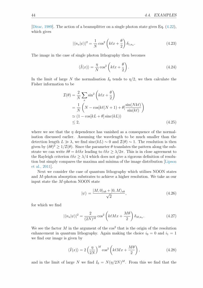
44 4.4. EXAMPLES
[Dirac, 1989]. The action of a beamsplitter on a single photon state gives Eq. (4.22),which gives
|〈nx|ψ〉|2 =1
Ncos2
(k`x+
θ
2
)δ1,nx . (4.23)
The image in the case of single photon lithography then becomes
〈I(x)〉 =η
Ncos2
(k`x+
θ
2
). (4.24)
In the limit of large N the normalisation I0 tends to η/2, we then calculate theFisher information to be
I(θ) =2
N
∑
x
sin2
(k`x+
θ
2
)
=1
N
(N − cos[k`(N + 1) + θ]
sin(Nk`)
sin(k`)
)
' (1− cos[kL+ θ] sinc(kL))
≤ 2, (4.25)
where we see that the η dependence has vanished as a consequence of the normal-isation discussed earlier. Assuming the wavelength to be much smaller than thedetection length L λ, we find sinc(kL) ∼ 0 and I(θ) ∼ 1. The resolution is thengiven by (δθ)2 ≥ 1/I(θ). Since the parameter θ translates the pattern along the sub-strate we can write δθ = k`δx leading to `δx ≥ λ/2π. This is in close agreement tothe Rayleigh criterion `δx ≥ λ/4 which does not give a rigorous definition of resolu-tion but simply compares the maxima and minima of the image distribution [Lipsonet al., 2011].
Next we consider the case of quantum lithography which utilises NOON statesand M -photon absorption substrates to achieve a higher resolution. We take as ourinput state the M -photon NOON state
|ψ〉 =|M, 0〉ab + |0,M〉ab√
2, (4.26)
for which we find
|〈nx|ψ〉|2 =2
(2N)Mcos2
(k`Mx+
Mθ
2
)δM,nx . (4.27)
We see the factor M in the argument of the cos2 that is the origin of the resolutionenhancement in quantum lithography. Again making the choice i0 = 0 and i1 = 1we find our image is given by
〈I(x)〉 = 2( η
2N
)Mcos2
(k`Mx+
Mθ
2
), (4.28)
and in the limit of large N we find I0 = N(η/2N)M . From this we find that the
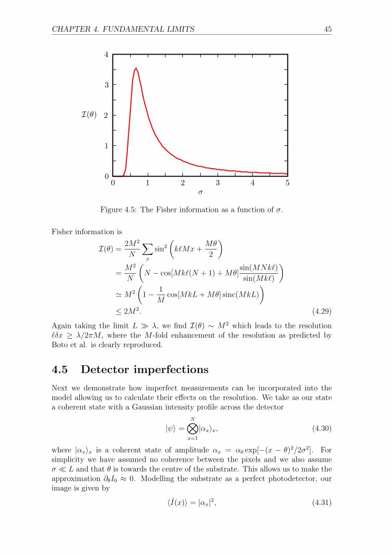
CHAPTER 4. FUNDAMENTAL LIMITS 45
Figure 4.5: The Fisher information as a function of σ.
Fisher information is
I(θ) =2M2
N
∑
x
sin2
(k`Mx+
Mθ
2
)
=M2
N
(N − cos[Mk`(N + 1) +Mθ]
sin(MNk`)
sin(Mk`)
)
'M2
(1− 1
Mcos[MkL+Mθ] sinc(MkL)
)
≤ 2M2. (4.29)
Again taking the limit L λ, we find I(θ) ∼ M2 which leads to the resolution`δx ≥ λ/2πM , where the M -fold enhancement of the resolution as predicted byBoto et al. is clearly reproduced.
4.5 Detector imperfections
Next we demonstrate how imperfect measurements can be incorporated into themodel allowing us to calculate their effects on the resolution. We take as our statea coherent state with a Gaussian intensity profile across the detector
|ψ〉 =N⊗
x=1
|αx〉x, (4.30)
where |αx〉x is a coherent state of amplitude αx = α0 exp[−(x − θ)2/2σ2]. Forsimplicity we have assumed no coherence between the pixels and we also assumeσ L and that θ is towards the centre of the substrate. This allows us to make theapproximation ∂θI0 ≈ 0. Modelling the substrate as a perfect photodetector, ourimage is given by
〈I(x)〉 = |αx|2, (4.31)
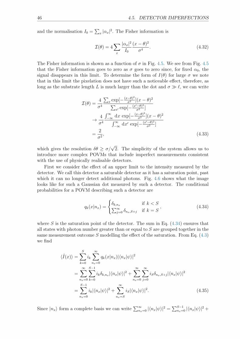
46 4.5. DETECTOR IMPERFECTIONS
and the normalisation I0 =∑
x |αx|2. The Fisher information is
I(θ) = 4∑
x
|αx|2I0
(x− θ)2
σ4. (4.32)
The Fisher information is shown as a function of σ in Fig. 4.5. We see from Fig. 4.5that the Fisher information goes to zero as σ goes to zero since, for fixed α0, thesignal disappears in this limit. To determine the form of I(θ) for large σ we notethat in this limit the pixelation does not have such a noticeable effect, therefore, aslong as the substrate length L is much larger than the dot and σ `, we can write
I(θ) =4
σ4
∑x exp[− (x−θ)2
σ2 ](x− θ)2
∑x′ exp[− (x′−θ)2
σ2 ]
→ 4
σ4
∫∞−∞ dx exp[− (x−θ)2
σ2 ](x− θ)2
∫∞−∞ dx′ exp[− (x′−θ)2
σ2 ]
=2
σ2, (4.33)
which gives the resolution δθ ≥ σ/√
2. The simplicity of the system allows us tointroduce more complex POVMs that include imperfect measurements consistentwith the use of physically realisable detectors.
First we consider the effect of an upper limit to the intensity measured by thedetector. We call this detector a saturable detector as it has a saturation point, pastwhich it can no longer detect additional photons. Fig. 4.6 shows what the imagelooks like for such a Gaussian dot measured by such a detector. The conditionalprobabilities for a POVM describing such a detector are
qk(x|nx) =
δk,nx if k < S∑∞
j=0 δnx,S+j if k = S, (4.34)
where S is the saturation point of the detector. The sum in Eq. (4.34) ensures thatall states with photon number greater than or equal to S are grouped together in thesame measurement outcome S modelling the effect of the saturation. From Eq. (4.3)we find
〈I(x)〉 =S∑
k=0
ik
∞∑
nx=0
qk(x|nx)|〈nx|ψ〉|2
=∞∑
nx=0
S−1∑
k=0
ikδk,nx|〈nx|ψ〉|2 +∞∑
nx=0
∞∑
j=0
iSδnx,S+j|〈nx|ψ〉|2
=S−1∑
nx=0
ik|〈nx|ψ〉|2 +∞∑
nx=S
iS|〈nx|ψ〉|2. (4.35)
Since |nx〉 form a complete basis we can write∑∞
nx=0 |〈nx|ψ〉|2 =∑S−1
nx=0 |〈nx|ψ〉|2 +

CHAPTER 4. FUNDAMENTAL LIMITS 47
Figure 4.6: A Gaussian intensity distribution as measured by a detector with asaturation point. The effect of the saturation is to chop the top of the Gaussiandistribution.
∑∞nx=S |〈nx|ψ〉|2 = 1 and the image is therefore
〈I(x)〉 =S−1∑
nx=0
ik|〈nx|ψ〉|2 + iS
(1−
S−1∑
nx=0
|〈nx|ψ〉|2)
=S−1∑
nx=0
(ik − iS)|〈nx|ψ〉|2 + iS. (4.36)
For the state given by Eq. (4.30) we find
|〈nx|ψ〉|2 = e−|αx|2 |αx|2nxnx!
(4.37)
and the probability distribution Pr(x|θ) is
Pr(x|θ) =
S−1∑nx=0
i0(nx − S)e−|αx|2 |αx|2nx
nx!+ i0S
∑x
S−1∑nx=0
i0(nx − S)e−|αx|2 |αx|2nx
nx!+ i0S
=
S−1∑nx=0
(nx − S)e−|αx|2 |αx|2nx
nx!+ S
∑x
S−1∑nx=0
(nx − S)e−|αx|2 |αx|2nx
nx!+ S
, (4.38)
where we have defined i0 ≡ ik/k to be the image intensity per photon. We againmake the assumption that the image normalisation I0 is independent of θ. The
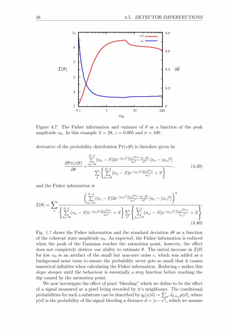
48 4.5. DETECTOR IMPERFECTIONS
Figure 4.7: The Fisher information and variance of θ as a function of the peakamplitude α0. In this example S = 28, ε = 0.005 and σ = 100.
derivative of the probability distribution Pr(x|θ) is therefore given by
∂Pr(x|θ)∂θ
=
S−1∑nx=0
(nx − S)2e−|αx|2 |αx|2nx
nx!(x−θ)σ2 [nx − |αx|2]
∑x
S−1∑nx=0
(nx − S)e−|αx|2 |αx|2nx
nx!+ S
, (4.39)
and the Fisher information is
I(θ) =∑
x
(S−1∑nx=0
(nx − S)2e−|αx|2 |αx|2nx
nx!(x−θ)σ2 [nx − |αx|2]
)2
S−1∑nx=0
(nx − S)e−|αx|2 |αx|2nx
nx!+ S
∑x′
S−1∑nx′=0
(nx′ − S)e−|αx′ |2 |αx′ |2nx′
nx′ !+ S
.
(4.40)
Fig. 4.7 shows the Fisher information and the standard deviation δθ as a functionof the coherent state amplitude α0. As expected, the Fisher information is reducedwhen the peak of the Gaussian reaches the saturation point, however, the effectdoes not completely destroy our ability to estimate θ. The initial increase in I(θ)for low α0 is an artefact of the small but non-zero noise ε, which was added as abackground noise term to ensure the probability never gets so small that it causesnumerical infinities when calculating the Fisher information. Reducing ε makes thisslope steeper until the behaviour is essentially a step function before reaching thedip caused by the saturation point.
We now investigate the effect of pixel “bleeding” which we define to be the effectof a signal measured at a pixel being recorded by it’s neighbours. The conditionalprobabilities for such a substrate can be described by qk(x|~n) =
∑x′ δk,nx′p(d), where
p(d) is the probability of the signal bleeding a distance d = |x−x′|, which we assume

CHAPTER 4. FUNDAMENTAL LIMITS 49
Figure 4.8: The Fisher information as a function of the pixel bleeding b.
to be symmetric. The image for such a detector is
〈I(x)〉 =∑
x′
i0p(|x− x′|)|αx′|2, (4.41)
and, assuming again ∂θI0 = 0, the Fisher information is
I(θ) =∑
x1
(∑x2
2p(|x1 − x2|)(x2 − θ) |αx2 |2
σ2
)2
∑x3
p(|x1 − x3|)|αx3|2 ∑
x4,x5
p(|x4 − x5|)|αx5|2 . (4.42)
For simplicity we take as our probability distribution p(|x − x′|) a Poissonian withbleeding parameter b which characterises the average distance that the signal bleeds.This gives us
p(|x− x′|) =1
p0
b|x−x′|e−b
|x− x′| , (4.43)
where
p0 =∑
x′′
b|x−x′′|e−b
|x− x′′| , (4.44)
which ensures that the probability is normalised despite the finite size of the sub-strate. Since the parameter α0 appears to the fourth power in both the numeratorand denominator of Eq. (4.42). The plot shows that the Fisher information is de-creased as the bleeding parameter b is increased. Fig. 4.8 shows the variation in theFisher information as a function of b.
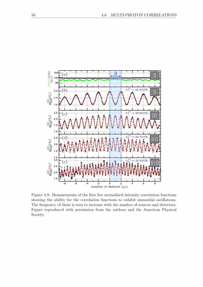
50 4.6. MULTI-PHOTON CORRELATIONS
detection time windows and higher single photon countingrates at the N detectors. From the figure it can be seen
that the measured curves for gð3ÞTLSð!1Þ, gð4ÞTLSð!1Þ, and
gð5ÞTLSð!1Þ display a doubled (2!1), tripled (3!1), and quad-rupled (4!1) modulation frequency with respect to
gð2ÞTLSð!1; 0Þ and gð2ÞSPEð!1; 0Þ [see Eqs. (5) and (8)]. Thismeans that for a given aperture A (indicated in Fig. 4)
gð5ÞTLSð!1Þ exhibits 4 times more oscillations than gð2ÞTLSð!1Þ.According to Eq. (2), this beats the classical Abbe limit for!d by a factor of 4.
In conclusion, we experimentally demonstrated spatialmultiphoton interference patterns displaying superresolu-tion with up to five statistically independent light sourcesby using linear optical detection techniques. For N > 2,these experiments achieve a higher resolution than theclassical Abbe limit for imaging the light source. In thecase of N SPE, we showed theoretically that the inter-ference pattern obtained is identical to the one generatedby NOON states with N # 1 photons, although the typesof interference are fundamentally different [23]. Using NTLS leads to the same NOON-like modulation, although
with a reduced visibility. Unlike for NOON states, ourtechnique requires neither special quantum tailoring oflight nor N-photon absorbing media, as it relies on singlephoton detection only. As intensity correlations of orderN > 2 are used to improve the spatial resolution inimaging, it can be regarded an extension of the HanburyBrown–Twiss experiment, one of the fundamental mea-surement techniques in quantum optics. The natural lowlight requirements suggest that the technique has potentialapplications for improved imaging of faint star clusters andin vivo biological samples.The authors thank I. Harder for the fabrication of the
masks and G. S. Agarwal, F. Schmidt-Kaler, A. Ramsay,A. Maser, U. Schilling, and R. Wiegner for critical dis-cussions. The authors gratefully acknowledge funding bythe Universitatsbund Erlangen-Nurnberg e.V., the ErlangenGraduate School in Advanced Optical Technologies(SAOT) by the German Research Foundation (DFG) inthe framework of the German excellence initiative andthe United Kingdom Engineering and Physical SciencesResearch Council. S. O. thanks the Elite Network ofBavaria for financial support.
*[email protected][1] E. Knill, R. Laflamme, and G. J. Milburn, Nature
(London) 409, 46 (2001).[2] P. Kok and B.W. Lovett, Introduction to Optical Quantum
Information Processing (Cambridge University Press,Cambridge, England, 2010).
[3] D. L. Moehring, P. Maunz, S. Olmschenk, K. C. Younge,D. N. Matsukevich, L.-M. Duan, and C. Monroe, Nature(London) 449, 68 (2007).
[4] S. Olmschenk, D. N. Matsukevich, P. Maunz, D. Hayes,L.-M. Duan, and C. Monroe, Science 323, 486 (2009).
[5] Y. Shih, Advances in Laser & Electro Optics, edited byN. Costa and A. Cartaxo (InTech, Vukovar, 2010).
[6] B. I. Erkmen and J. H. Shapiro, Adv. Opt. Photon. 2, 405(2010).
[7] V. Giovannetti, S. Lloyd, and L. Maccone, Nat. Photonics5, 222 (2011).
[8] A. N. Boto, P. Kok, D. S. Abrams, S. L. Braunstein, C. P.Williams, and J. P. Dowling, Phys. Rev. Lett. 85, 2733(2000).
[9] D. Leibfried M.D. Barrett, T. Schaetz, J. Britton, J.Chiaverini, W.M. Itano, J. D. Jost, C. Langer, and D. J.Wineland, Science 304, 1476 (2004).
[10] M. D’Angelo, M.V. Chekhova, and Y. Shih, Phys. Rev.Lett. 87, 013602 (2001).
[11] P. Walther, J.-W. Pan, M. Aspelmeyer, R. Ursin, S.Gasparoni, and A. Zeilinger, Nature (London) 429, 158(2004).
[12] M.W. Mitchell, J. S. Lundeen, and A.M. Steinberg,Nature (London) 429, 161 (2004).
[13] R. Hanbury Brown and R.Q. Twiss, Nature (London) 177,27 (1956).
[14] A. Muthukrishnan, M.O. Scully, and M. S. Zubairy,J. Opt. B 6, S575 (2004).
FIG. 4 (color online). Experimental results: (a) Measurementof average intensities I1 and I2 at detectors D1 and D2 alone(with D1 scanned and D2 kept constant), demonstrating thatthe pseudothermal light used is spatially incoherent in first order
of the intensity. (b)–(e) Measurement of gðNÞTLSð!1Þ in the case of
N ¼ 2; . . . ; 5 TLS for !2; . . . ;!N at the magic positions. Solidred curves correspond to a theoretical fit taking into account thefinite width of the slits. The only fitting parameters are the slit
separation d, the slit width a, and the visibility VðeÞN . The
experimentally obtained visibilities VðeÞN can be compared with
the theoretical values VN in Fig. 1.
PRL 109, 233603 (2012) P HY S I CA L R EV I EW LE T T E R Sweek ending
7 DECEMBER 2012
233603-4
Figure 4.9: Measurements of the first five normalised intensity correlation functionsshowing the ability for the correlation functions to exhibit sinusoidal oscillations.The frequency of these is seen to increase with the number of sources and detectors.Figure reproduced with permission from the authors and the American PhysicalSociety.
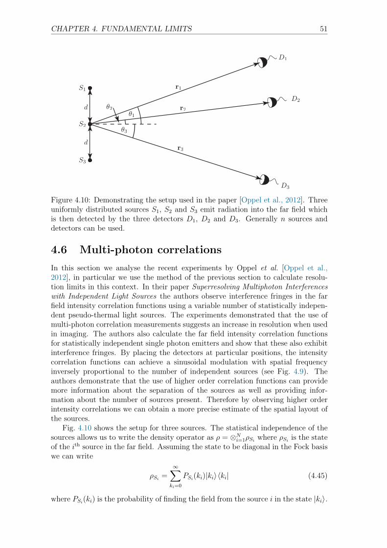
CHAPTER 4. FUNDAMENTAL LIMITS 51
Figure 4.10: Demonstrating the setup used in the paper [Oppel et al., 2012]. Threeuniformly distributed sources S1, S2 and S3 emit radiation into the far field whichis then detected by the three detectors D1, D2 and D3. Generally n sources anddetectors can be used.
4.6 Multi-photon correlations
In this section we analyse the recent experiments by Oppel et al. [Oppel et al.,2012], in particular we use the method of the previous section to calculate resolu-tion limits in this context. In their paper Superresolving Multiphoton Interferenceswith Independent Light Sources the authors observe interference fringes in the farfield intensity correlation functions using a variable number of statistically indepen-dent pseudo-thermal light sources. The experiments demonstrated that the use ofmulti-photon correlation measurements suggests an increase in resolution when usedin imaging. The authors also calculate the far field intensity correlation functionsfor statistically independent single photon emitters and show that these also exhibitinterference fringes. By placing the detectors at particular positions, the intensitycorrelation functions can achieve a sinusoidal modulation with spatial frequencyinversely proportional to the number of independent sources (see Fig. 4.9). Theauthors demonstrate that the use of higher order correlation functions can providemore information about the separation of the sources as well as providing infor-mation about the number of sources present. Therefore by observing higher orderintensity correlations we can obtain a more precise estimate of the spatial layout ofthe sources.
Fig. 4.10 shows the setup for three sources. The statistical independence of thesources allows us to write the density operator as ρ = ⊗Ni=1ρSi where ρSi is the stateof the ith source in the far field. Assuming the state to be diagonal in the Fock basiswe can write
ρSi =∞∑
ki=0
PSi(ki)|ki〉〈ki| (4.45)
where PSi(ki) is the probability of finding the field from the source i in the state |ki〉.

52 4.6. MULTI-PHOTON CORRELATIONS
By the superposition principle the electric field operators in the far field, E(r) willbe a sum of the field operators from each of the sources S1(r), . . . , SN(r). Writingthe operator G = E(+)(r1) . . . E(+)(rn) for shorthand 1, we can write
G =n∏
i=1
E(+)(ri)
=n∏
i=1
[S(+)1 (ri) + · · ·+ S
(+)N (ri)] (4.46)
where S(+)j (ri) is proportional to the photon annihilation operator at the point ri
from the source Sj. The n-point intensity correlation can be calculated as follows
G(n)(r1, . . . , rn)
= Tr[ρG]
= Tr
[ ∞∑
k1=0
· · ·∞∑
kN=0
PS1(k1) . . . PSN (kN)|k1, . . . , kN〉〈k1, . . . , kN |G†G]
=∞∑
k1=0
· · ·∞∑
kN=0
PS1(k1) . . . PSN (kN)〈k1, . . . , kN |G†G|k1, . . . , kN〉
=∞∑
k1=0
· · ·∞∑
kN=0
PS1(k1) . . . PSN (kN)∞∑
m1=0
· · ·∞∑
mN=0
|〈m1, . . . ,mN |G|k1, . . . , kN〉|2.
(4.47)
Writing Sj(+)
(ri) = κeikrji aSj , where rji is the distance from the jth source to ith
detector, we can calculate the normalised intensity correlation explicitly for N = 2and 3. The factor κ is strictly a function of the geometry of the arrangement.However, in the far field, paraxial regime, κ can be considered a constant. First wemust calculate G(1)(r1) for N = 2 and 3
G(1)(r1) =∞∑
k1=0
∞∑
k2=0
∞∑
m1=0
∞∑
m2=0
PS1(k1)PS2(k2)|〈m1,m2|S(+)1 (r1) + S
(+)2 (r1)|k1, k2〉|2
=∞∑
k1=0
∞∑
k2=0
PS1(k1)PS2(k2)
[|〈k1 − 1, k2|S(+)
1 (r1)|k1, k2〉|2
+ |〈k1, k2 − 1|S(+)2 (r1)|k1, k2〉|2
]
=∞∑
k1=0
∞∑
k2=0
PS1(k1)PS2(k2)κ[k1 + k2]
= κ[〈n1〉+ 〈n2〉] (4.48)
where 〈ni〉 is the photon number expectation associated with source i. Likewise forN = 3, G(1)(r1) = κ〈n1〉 + 〈n2〉 + 〈n3〉. The second order intensity correlation is
1We use N for the total number of sources and n for the number of detectors. These do notnecessarily have to be the same although in the experiments performed by Oppel et al. N = nwas used throughout.

CHAPTER 4. FUNDAMENTAL LIMITS 53
calculated to be
G(2)(r1, r2) =∞∑
k1=0
∞∑
k2=0
∞∑
m1=0
∞∑
m2=0
PS1(k1)PS2(k2)|〈m1,m2|[S(+)1 (r1) + S
(+)2 (r1)]
× [S(+)1 (r2) + S
(+)2 (r2)]|k1, k2〉|2. (4.49)
In general all the terms in the expansion of the square brackets will contribute tothe correlation function.
Using for the sources single photon emitters (SPE) and thermal light sources(TLS), we find the probabilities PSi(kj) are given by
SPE : PSi(kj) =
1 if kj = 1
0 if kj 6= 1(4.50)
TLS : PSi(kj) =〈ni〉kj
(1 + 〈ni〉)kj+1, (4.51)
where the distribution for the TLS sources is the well known Bose-Einstein distri-bution. The sources are treated as point like, therefore justifying the assumptionthat the thermal light sources consist of a single mode in thermal equilibrium.
4.6.1 Single photon sources
For single photon sources, we find by inserting Eq. (4.50) into Eq. (4.49) we find
G(2)SPE(r1, r2) = |〈k1 − 1, k2 − 1|[S(+)
1 (r2)S(+)2 (r1) + S
(+)1 (r1)S
(+)2 (r2)]|k1, k2〉|2
= κ2|eik(r21+r12) + eik(r11+r22)|2
= κ2[2 + eik(r21+r12−r11−r22) + e−ik(r21+r12−r11−r22)
]
= κ2 [2 + 2 cos(kd sinφ1 − kd sinφ2)]
≡ κ2 [2 + 2 cos(δ1 − δ2)] , (4.52)
where we have defined δi = kθ sinφi, φi being the angle between the central normalto the sources and the source i and θ being the separation between the two sources.Using Eq. (4.48) we find
g(2)SPE(δ1, δ2) =
1
2[1 + cos(δ1 − δ2)], (4.53)
where we see the appearance of a sinusoidal oscillation of the correlation functionwith spatial frequency kd and we have changed the arguments to δ1, δ2 for clarity.
Since the correlation functions depend on all the possible indistinguishable pathsthat the emitted photons can take to arrive at the detector the general expressionfor the correlation functions grows factorially with n. For single photon sources thethird order correlation is
g(3)SPE(r1, r2, r3) =
2
27
[3 + 2 cos(δ1 − δ2) + 2 cos(δ1 − δ3) + 2 cos(δ2 − δ3)
+ cos(2δ1 − 2δ2) + cos(2δ1 − 2δ3) + cos(2δ2 − 2δ3)
+ 2 cos(2δ1 − δ2 − δ3) + cos(δ1 + δ2 − 2δ3) + cos(−δ1 + 2δ2 − δ3)
+ cos(δ1 + δ2 − 2δ3) + cos(δ1 − 2δ2 − δ3)
], (4.54)
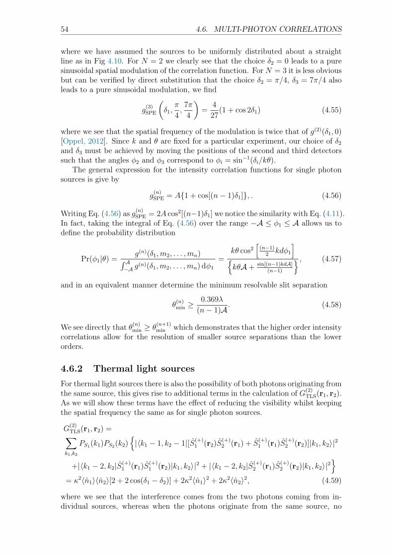
54 4.6. MULTI-PHOTON CORRELATIONS
where we have assumed the sources to be uniformly distributed about a straightline as in Fig 4.10. For N = 2 we clearly see that the choice δ2 = 0 leads to a puresinusoidal spatial modulation of the correlation function. For N = 3 it is less obviousbut can be verified by direct substitution that the choice δ2 = π/4, δ3 = 7π/4 alsoleads to a pure sinusoidal modulation, we find
g(3)SPE
(δ1,
π
4,7π
4
)=
4
27(1 + cos 2δ1) (4.55)
where we see that the spatial frequency of the modulation is twice that of g(2)(δ1, 0)[Oppel, 2012]. Since k and θ are fixed for a particular experiment, our choice of δ2
and δ3 must be achieved by moving the positions of the second and third detectorssuch that the angles φ2 and φ3 correspond to φi = sin−1(δi/kθ).
The general expression for the intensity correlation functions for single photonsources is give by
g(n)SPE = A1 + cos[(n− 1)δ1], . (4.56)
Writing Eq. (4.56) as g(n)SPE = 2A cos2[(n−1)δ1] we notice the similarity with Eq. (4.11).
In fact, taking the integral of Eq. (4.56) over the range −A ≤ φ1 ≤ A allows us todefine the probability distribution
Pr(φ1|θ) =g(n)(δ1,m2, . . . ,mn)∫ A
−A g(n)(δ1,m2, . . . ,mn) dφ1
=kθ cos2
[(n−1)
2kdφ1
]
kθA+ sin[(n−1)kdA]
(n−1)
, (4.57)
and in an equivalent manner determine the minimum resolvable slit separation
θ(n)min ≥
0.369λ
(n− 1)A . (4.58)
We see directly that θ(n)min ≥ θ
(n+1)min which demonstrates that the higher order intensity
correlations allow for the resolution of smaller source separations than the lowerorders.
4.6.2 Thermal light sources
For thermal light sources there is also the possibility of both photons originating fromthe same source, this gives rise to additional terms in the calculation of G
(2)TLS(r1, r2).
As we will show these terms have the effect of reducing the visibility whilst keepingthe spatial frequency the same as for single photon sources.
G(2)TLS(r1, r2) =∑
k1,k2
PS1(k1)PS2(k2)|〈k1 − 1, k2 − 1|[S(+)
1 (r2)S(+)2 (r1) + S
(+)1 (r1)S
(+)2 (r2)]|k1, k2〉|2
+|〈k1 − 2, k2|S(+)1 (r1)S
(+)1 (r2)|k1, k2〉|2 + |〈k1 − 2, k2|S(+)
2 (r1)S(+)2 (r2)|k1, k2〉|2
= κ2〈n1〉〈n2〉[2 + 2 cos(δ1 − δ2)] + 2κ2〈n1〉2 + 2κ2〈n2〉2, (4.59)
where we see that the interference comes from the two photons coming from in-dividual sources, whereas when the photons originate from the same source, no

CHAPTER 4. FUNDAMENTAL LIMITS 55
10
20
30
40
50
60
Figure 4.11: The resolution of the correlation functions against the correlation ordern.
interference occurs. Assuming the sources to be equal intensities, 〈n1〉 = 〈n2〉 ≡ 〈n〉we find the normalised intensity correlation to be
g(2)TLS(δ1, δ2) =
3
2
[1 +
1
3cos(δ1 − δ2)
]. (4.60)
We see from Eq. (4.60) that the spatial modulation of the correlation function isthe same as for the single photon sources, however the visibility is reduced by 70%.There is a clear interpretation of this reduction in the visibility, since it is caused bythe terms that account for the two photons originating from the same source whichclearly carry no information about the spatial separation of the two independentsources.
Remarkably, as we observed for g(2), the third order correlation for thermal lightsources can also exhibit a pure sinusoidal oscillation of the same spatial frequencyas g
(3)TLS. As with the second order correlation the visibility for thermal light sources
is reduced compared with the single photon emitters. In order to obtain a puresinusoidal modulation for thermal light sources, we must choose δ2 = 0 and δ3 = π.For an appropriate choice δ2 . . . δn we find that the intensity correlations for thermallight sources can be described by the expression
g(n)TLS = B1 + Vn cos[(n− 1)δ1]. (4.61)
For thermal light sources the appearance of Vn in Eq. (4.61) does not allow us toderive a similar analytic expression for the minimum resolvable source separation.However we can numerically find the resolution for various orders of n. Fig. 4.11shows the resolution as a function of n, we see that the single photon emitting sourcesalways provide better resolution compared to the thermal light sources, however, thegeneral trend of the resolution decreasing with n is still present even for thermalsources.

56 4.7. DISCUSSION AND CONCLUSIONS
4.7 Discussion and conclusions
In conclusion, we have demonstrated how the statistical distance can be used asa measure of distinguishability for probability distributions. By identifying imageswith probability distributions we have shown how the statistical distance can beused to determine the resolution of various imaging procedures. Detector imper-fections can be fully accounted for and the resolution of various setups includingimperfections can be calculated via this method. By identifying an image with theexpectation value of the imaging observable we ignore the effects of noise in thedetection. In order to properly perform a parameter estimation of the spatial pa-rameters of the source we must take noise into account. This is the topic of the nextchapter.
Chapter 5
Estimation of Thermal SourceDimensions
The contents of this chapter is based on [Pearce et al., 2015]. In this chapter we userigorous estimation theory to demonstrate how higher-order intensity interferometrycan yield a resolution improvement over the lowest (second) order intensity interfer-ometry. The general setup is shown in Fig. 5.1a. We provide a general frameworkthat allows us to analyse intensity correlations of arbitrary order and discuss the ad-vantages and disadvantages associated with higher-order intensity correlations. Wepresent a rigorous analysis of the HBT set up, explicitly calculating the likelihoodfunction and Fisher information, which allows us to determine the lowest possi-ble variance in estimates of the source and also allows us to perform a maximumlikelihood estimation, therefore achieving this bound. An integral part of our proce-dure is to treat unknown quantities as parameters to be estimated, every unknowntherefore increasing the size of the estimation problem. We then demonstrate ourmethod, making use of simulated data to obtain precision estimates of the radiusof a thermal source. We also show how these results can be used to estimate thedimensions of any source, regardless of its geometry. Our method is also not limitedto thermal sources. We show that as long as the total photon number is not deter-ministic (i.e. ∆n > 0) our method can be used to calculate the Fisher informationand also provide maximum likelihood estimates of the source dimensions via themethod of scoring.
By explicitly calculating the Fisher information for different correlation ordersn, we show that in some instances the Fisher information increases with correlationorder. However the exact relationship between the Fisher information and the cor-relation order depends strongly on the particular arrangement of the detectors andthe source geometry. The idea of exploiting higher order intensity correlations toimprove resolution has been suggested previously [Thiel et al., 2007, Oppel et al.,2012,Iskhakov et al., 2011] and in the context of ghost imaging, the idea of exploitinghigher correlation orders has received great attention [Zhou et al., 2010,Chen et al.,2010,Chan et al., 2009,Agafonov et al., 2009b]. However, to date there has not beena rigorous theoretical explanation which can quantify the possible enhancement ofhigher order correlation measurements for HBT-type experiments. We provide thatexplanation here and demonstrate its use. We also include the effects of photonlosses in our model and show that higher order correlation can continue to performwell even in the presence of loss.
57
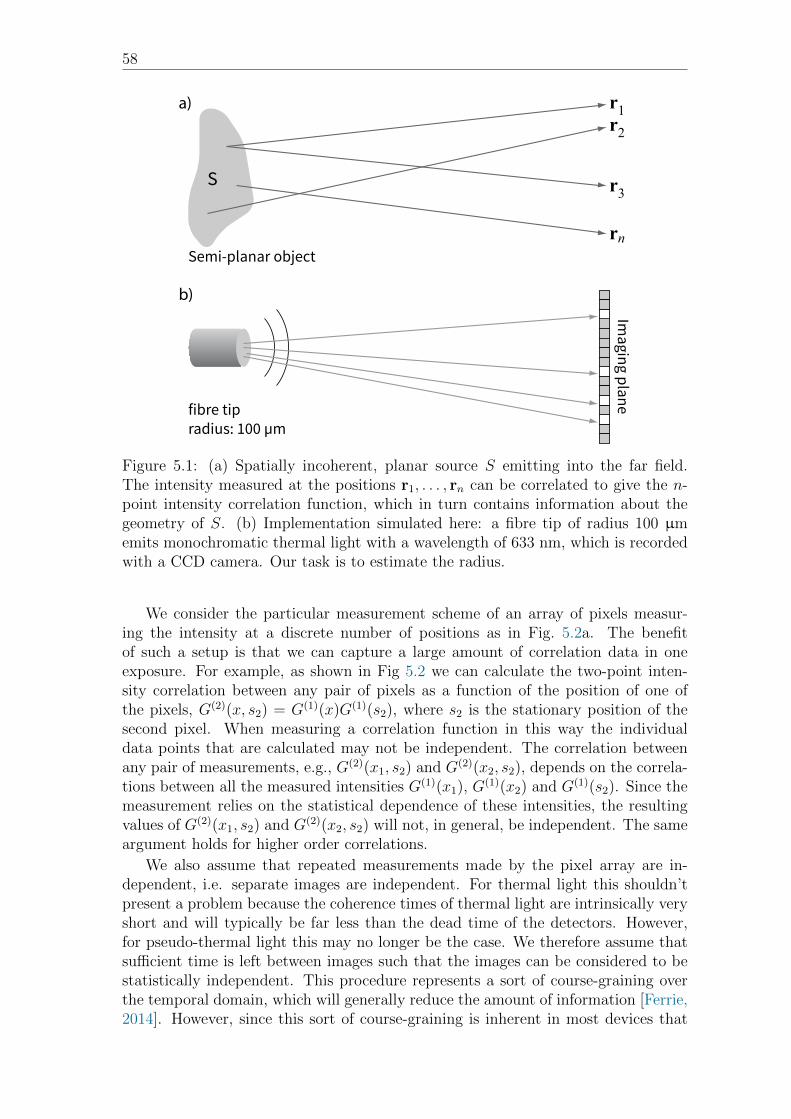
58
r
1
r
rr
n
3
2
Semi-planar object
Imaging plane
S
fibre tipradius: 100 µm
a)
b)
Figure 5.1: (a) Spatially incoherent, planar source S emitting into the far field.The intensity measured at the positions r1, . . . , rn can be correlated to give the n-point intensity correlation function, which in turn contains information about thegeometry of S. (b) Implementation simulated here: a fibre tip of radius 100 µmemits monochromatic thermal light with a wavelength of 633 nm, which is recordedwith a CCD camera. Our task is to estimate the radius.
We consider the particular measurement scheme of an array of pixels measur-ing the intensity at a discrete number of positions as in Fig. 5.2a. The benefitof such a setup is that we can capture a large amount of correlation data in oneexposure. For example, as shown in Fig 5.2 we can calculate the two-point inten-sity correlation between any pair of pixels as a function of the position of one ofthe pixels, G(2)(x, s2) = G(1)(x)G(1)(s2), where s2 is the stationary position of thesecond pixel. When measuring a correlation function in this way the individualdata points that are calculated may not be independent. The correlation betweenany pair of measurements, e.g., G(2)(x1, s2) and G(2)(x2, s2), depends on the correla-tions between all the measured intensities G(1)(x1), G(1)(x2) and G(1)(s2). Since themeasurement relies on the statistical dependence of these intensities, the resultingvalues of G(2)(x1, s2) and G(2)(x2, s2) will not, in general, be independent. The sameargument holds for higher order correlations.
We also assume that repeated measurements made by the pixel array are in-dependent, i.e. separate images are independent. For thermal light this shouldn’tpresent a problem because the coherence times of thermal light are intrinsically veryshort and will typically be far less than the dead time of the detectors. However,for pseudo-thermal light this may no longer be the case. We therefore assume thatsufficient time is left between images such that the images can be considered to bestatistically independent. This procedure represents a sort of course-graining overthe temporal domain, which will generally reduce the amount of information [Ferrie,2014]. However, since this sort of course-graining is inherent in most devices that
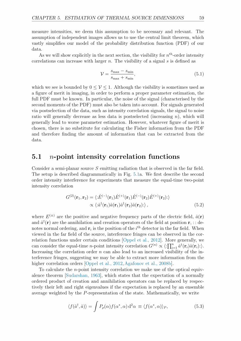
CHAPTER 5. ESTIMATION OF THERMAL SOURCE DIMENSIONS 59
measure intensities, we deem this assumption to be necessary and relevant. Theassumption of independent images allows us to use the central limit theorem, whichvastly simplifies our model of the probability distribution function (PDF) of ourdata.
As we will show explicitly in the next section, the visibility for nth-order intensitycorrelations can increase with larger n. The visibility of a signal s is defined as
V =smax − smin
smax + smin
, (5.1)
which we see is bounded by 0 ≤ V ≤ 1. Although the visibility is sometimes used asa figure of merit in imaging, in order to perform a proper parameter estimation, thefull PDF must be known. In particular, the noise of the signal (characterised by thesecond moments of the PDF) must also be taken into account. For signals generatedvia postselection of the data, such as intensity correlation signals, the signal to noiseratio will generally decrease as less data is postselected (increasing n), which willgenerally lead to worse parameter estimation. However, whatever figure of merit ischosen, there is no substitute for calculating the Fisher information from the PDFand therefore finding the amount of information that can be extracted from thedata.
5.1 n-point intensity correlation functions
Consider a semi-planar source S emitting radiation that is observed in the far field.The setup is described diagrammatically in Fig. 5.1a. We first describe the secondorder intensity interference for experiments that measure the equal-time two-pointintensity correlation
G(2)(r1, r2) = 〈:E(−)(r1)E(+)(r1)E(−)(r2)E(+)(r2):〉∝ 〈:a†(r1)a(r1)a†(r2)a(r2):〉 , (5.2)
where E(±) are the positive and negative frequency parts of the electric field, a(r)and a†(r) are the annihilation and creation operators of the field at position r, : : de-notes normal ordering, and ri is the position of the ith detector in the far field. Whenviewed in the far field of the source, interference fringes can be observed in the cor-relation functions under certain conditions [Oppel et al., 2012]. More generally, wecan consider the equal-time n-point intensity correlation G(n) ∝ 〈:∏n
i=1 a†(ri)a(ri):〉.
Increasing the correlation order n can also lead to an increased visibility of the in-terference fringes, suggesting we may be able to extract more information from thehigher correlation orders [Oppel et al., 2012,Agafonov et al., 2008b].
To calculate the n-point intensity correlation we make use of the optical equiv-alence theorem [Sudarshan, 1963], which states that the expectation of a normallyordered product of creation and annihilation operators can be replaced by respec-tively their left and right eigenvalues if the expectation is replaced by an ensembleaverage weighted by the P -representation of the state. Mathematically, we write
〈f(a†, a)〉 =
∫Pρ(α)f(α∗, α) d2α ≡ 〈f(α∗, α)〉P , (5.3)

60 5.1. N -POINT INTENSITY CORRELATION FUNCTIONS
1 7 2513 pixel number
17
2513
n = 2
a)
b) d)
c) e)
n = 3detection scheme 1
n = 3detection scheme 2
n = 4detection scheme 1
n = 4detection scheme 2
G (1)
G (2)
G (3) G (4)
G (3) G (4)
G (1) G (1)
G (1) G (1)
= correlate
output after post-processing data
measured data
Figure 5.2: Measuring the second order intensity correlation function with an arrayof pixels. (a) The second order intensity correlation G(2)(xi) at pixel xi = 7 iscalculated as the correlation between the intensities G(1)(s2) at a fixed pixel s2 = 13(shown as a darker pixel) and G(1)(xi) at the pixel xi = 7. (b, c) The third ordercorrelation function G(3)(xi) is defined using two detection schemes, namely via asingle fixed pixel that is correlated twice (detection scheme 1, note the double linefrom pixel 13), or two fixed pixels (detection scheme 2). (d, e) The fourth orderintensity correlation G(4)(xi) is defined analogous to G(3)(xi).
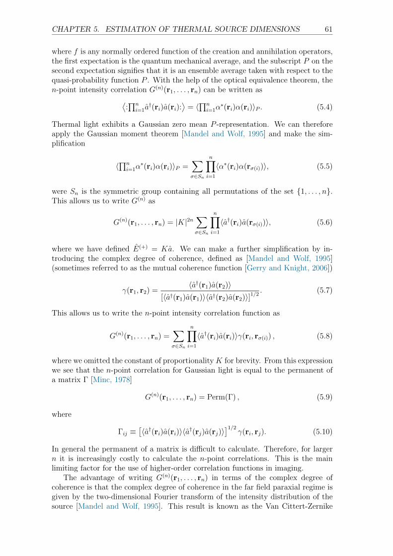
CHAPTER 5. ESTIMATION OF THERMAL SOURCE DIMENSIONS 61
where f is any normally ordered function of the creation and annihilation operators,the first expectation is the quantum mechanical average, and the subscript P on thesecond expectation signifies that it is an ensemble average taken with respect to thequasi-probability function P . With the help of the optical equivalence theorem, then-point intensity correlation G(n)(r1, . . . , rn) can be written as
⟨:∏n
i=1a†(ri)a(ri):
⟩= 〈∏n
i=1α∗(ri)α(ri)〉P . (5.4)
Thermal light exhibits a Gaussian zero mean P -representation. We can thereforeapply the Gaussian moment theorem [Mandel and Wolf, 1995] and make the sim-plification
〈∏ni=1α
∗(ri)α(ri)〉P =∑
σ∈Sn
n∏
i=1
〈α∗(ri)α(rσ(i))〉, (5.5)
were Sn is the symmetric group containing all permutations of the set 1, . . . , n.This allows us to write G(n) as
G(n)(r1, . . . , rn) = |K|2n∑
σ∈Sn
n∏
i=1
〈a†(ri)a(rσ(i))〉, (5.6)
where we have defined E(+) = Ka. We can make a further simplification by in-troducing the complex degree of coherence, defined as [Mandel and Wolf, 1995](sometimes referred to as the mutual coherence function [Gerry and Knight, 2006])
γ(r1, r2) =〈a†(r1)a(r2)〉
[〈a†(r1)a(r1)〉〈a†(r2)a(r2)〉]1/2. (5.7)
This allows us to write the n-point intensity correlation function as
G(n)(r1, . . . , rn) =∑
σ∈Sn
n∏
i=1
〈a†(ri)a(ri)〉γ(ri, rσ(i)) , (5.8)
where we omitted the constant of proportionality K for brevity. From this expressionwe see that the n-point correlation for Gaussian light is equal to the permanent ofa matrix Γ [Minc, 1978]
G(n)(r1, . . . , rn) = Perm(Γ) , (5.9)
where
Γij ≡[〈a†(ri)a(ri)〉〈a†(rj)a(rj)〉
]1/2γ(ri, rj). (5.10)
In general the permanent of a matrix is difficult to calculate. Therefore, for largern it is increasingly costly to calculate the n-point correlations. This is the mainlimiting factor for the use of higher-order correlation functions in imaging.
The advantage of writing G(n)(r1, . . . , rn) in terms of the complex degree ofcoherence is that the complex degree of coherence in the far field paraxial regime isgiven by the two-dimensional Fourier transform of the intensity distribution of thesource [Mandel and Wolf, 1995]. This result is known as the Van Cittert-Zernike

62 5.1. N -POINT INTENSITY CORRELATION FUNCTIONS
-640 -320 0 320 6400
5
10
15
20
25
x - s2
GHn
L Hx,s
2,...
,s2L
Ha.u
.L
Figure 5.3: The second (dashed), third (dotted) and fourth (solid) order intensitycorrelation functions of Eq. (5.12) as a function of the separation between the scan-ning pixel r1 = x and the reference pixel s2 for the remaining arguments, and withnormalised intensity 〈a†(ri)a(ri)〉 = 1 and ϑk = 64. The width of the curves isdirectly proportional to the angular diameter of the source a. The higher visibilitiesof G(3) and G(4) over G(2) suggest that higher-order correlations may outperformregular Hanbury Brown and Twiss estimation of the source diameter. Here we showrigorously using estimation theory that this can indeed be the case in some instances.
theorem [van Cittert, 1934, Zernike, 1938]. We can therefore calculate the far fieldintensity correlations for any source geometry, provided that we can determine theFourier transform of the intensity distribution.
As an example, consider a monochromatic, thermal, circular source of uniformintensity and angular diameter ϑ = tan−1(a/d) ≈ a/d where a is the diameter of thesource and d is the distance from the source to the observation plane. The far fieldcomplex degree of coherence is the two-dimensional Fourier transform of a circlewith radius a [Born and Wolf, 1980]
γ(r1, r2) =2J1 (ϑk|r1 − r2|)
(ϑk|r1 − r2|), (5.11)
where J1 is the first order Bessel function of the first kind and k is the wavenumber.The n-point correlation function then becomes
G(n)(r1, . . . , rn) =∑
σ∈Sn
n∏
i=1
〈a†(ri)a(ri)〉2J1
(ϑk|ri − rσ(i)|
)(ϑk|ri − rσ(i)|
) . (5.12)
Fig. 5.3 shows the second, third and fourth order correlation functions for a uniformdisc along a one-dimensional detector. We have seen previously that the n-pointcorrelation contains a large number of terms (the permanent contains a sum overthe symmetric group Sn giving n! terms). In practice this is what limits our abilityto calculate arbitrary correlation orders.

CHAPTER 5. ESTIMATION OF THERMAL SOURCE DIMENSIONS 63
5.2 Estimation from intensity correlations
In the previous section we saw that intensity correlation measurements in the farfield depend on the parameters describing the source geometry, and in this sectionwe examine how we can use these measurements to practically obtain spatial infor-mation about the source. To this end we employ parameter estimation theory, whichinvolves the use of an estimator θ that takes the measured data x = (x1, . . . , xM) inM measurements (the pixels in the detector) and returns estimates of the parametersof interest θ = (θ1, . . . , θl). In order to extract the spatial information in the mostefficient way, we can apply a maximum likelihood estimation procedure. Maximumlikelihood estimation relies on maximisation of the joint probability distribution ofour data, and we therefore need to characterise the probability distribution fromwhich the correlation functions are sampled [Kay, 1993].
Once we have determined the the conditional probability p(x|θ) of obtaining themeasurement outcomes x given the values of the parameters θ = (θ1, . . . , θl), we candetermine the performance of our estimates using the Cramer-Rao bound (CRB).The CRB provides a lower bound for the variance of our estimators in terms of theFisher information matrix
Var(θi) ≥ [I(θ)]−1ii , (5.13)
where I(θ) is the Fisher information matrix given by
[I(θ)]ij =∑
x
p(x|θ)
(∂ ln[p(x|θ)]
∂θi
)(∂ ln[p(x|θ)]
∂θj
), (5.14)
where the sum over x may be an integral if the values of xi form a continuum. Inpractice, intensity measurements in modern optical detectors yield a digital signalwith discrete values.
The exact probability distribution p(x|θ) of the correlation functions will be acomplicated expression depending on the number of images N—not to be confusedwith the number of pixels M in each image. However, since the measurements ofthe correlation functions are averages over a (preferably) large data set, the centrallimit theorem dictates that these measurements will be normally distributed [van derVaart, 1998]. Assuming that we make M measurements of the correlation functionsat M discrete detector positions, in the limit of large N the data will follow anM -dimensional normal distribution:
p(x|θ) =exp
(−1
2(x− µ(θ))TC−1(θ)(x− µ(θ))
)√
(2π)M |C(θ)|, (5.15)
where µ is the tuple of expectation values of the distribution at each of the samplingpoints: µT = (〈x1〉, . . . , 〈xM〉), T denotes the transpose, and C is the covariancematrix between pairs of measurements Cij = Cov(xi,xj) = 〈xixj〉 − 〈xi〉〈xj〉.
For a multivariate-normal distribution the elements of the Fisher informationmatrix are given by [Kay, 1993]
[I(θ)]ij =
(∂µ
∂θi
)T
C−1
(∂µ
∂θj
)+
1
2Tr
[C−1∂C
∂θiC−1∂C
∂θj
]
≡ [I1(θ)]ij + [I2(θ)]ij, (5.16)
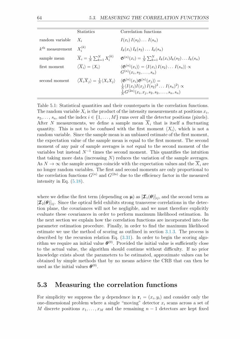
64 5.3. MEASURING THE CORRELATION FUNCTIONS
Statistics Correlation functions
random variable Xi I(xi) I(s2) . . . I(sn)
kth measurement X(k)i Ik(xi) Ik(s2) . . . Ik(sn)
sample mean Xi = 1N
∑Nk=1X
(k)i G(n)(xi) = 1
N
∑Nk=1 Ik(xi)Ik(s2) . . . Ik(sn)
first moment 〈Xi〉 = 〈Xi〉 〈G(n)(xi)〉 = 〈I(xi) I(s2) . . . I(sn)〉 ∝G(n)(xi, s2, . . . , sn)
second moment 〈XiXj〉 = 1N 〈XiXj〉 〈G(n)(xi)G
(n)(xj)〉 =1N 〈I(xi)I(xj) I(s2)2 . . . I(sn)2〉 ∝1NG
(2n)(xi, xj , s2, s2, . . . , sn, sn)
Table 5.1: Statistical quantities and their counterparts in the correlation functions.The random variable Xi is the product of the intensity measurements at positions xi,s2,. . . , sn, and the index i ∈ 1, . . . ,M runs over all the detector positions (pixels).After N measurements, we define a sample mean X i that is itself a fluctuatingquantity. This is not to be confused with the first moment 〈Xi〉, which is not arandom variable. Since the sample mean is an unbiased estimate of the first moment,the expectation value of the sample mean is equal to the first moment. The secondmoment of any pair of sample averages is not equal to the second moment of thevariables but instead N−1 times the second moment. This quantifies the intuitionthat taking more data (increasing N) reduces the variation of the sample averages.As N →∞ the sample averages coincide with the expectation values and the X i areno longer random variables. The first and second moments are only proportional tothe correlation functions G(n) and G(2n) due to the efficiency factor in the measuredintensity in Eq. (5.18).
where we define the first term (depending on µ) as [I1(θ)]ij, and the second term as[I2(θ)]ij. Since the optical field exhibits strong transverse correlations in the detec-tion plane, the covariances will not be negligible, and we must therefore explicitlyevaluate these covariances in order to perform maximum likelihood estimation. Inthe next section we explain how the correlation functions are incorporated into theparameter estimation procedure. Finally, in order to find the maximum likelihoodestimate we use the method of scoring as outlined in section 3.1.3. The process isdescribed by the recursion relation Eq. (3.31). In order to begin the scoring algo-rithm we require an initial value θ(0). Provided the initial value is sufficiently closeto the actual value, the algorithm should continue without difficulty. If no priorknowledge exists about the parameters to be estimated, approximate values can beobtained by simple methods that by no means achieve the CRB that can then beused as the initial values θ(0).
5.3 Measuring the correlation functions
For simplicity we suppress the y dependence in ri = (xi, yi) and consider only theone-dimensional problem where a single “moving” detector xi scans across a set ofM discrete positions x1, . . . , xM and the remaining n − 1 detectors are kept fixed
CHAPTER 5. ESTIMATION OF THERMAL SOURCE DIMENSIONS 65
(see Fig. 5.2b-e). We refer to the fixed detectors as the reference pixels and writethe reference pixel positions as x2 = s2, . . . , xn = sn. We distinguish betweentwo detector schemes, namely one where all reference pixels are identical (scheme1), and one where all reference pixels are different (scheme 2). Taking N imagesmeans performing N independent measurements of the intensity I(xi) at pixel xiand calculating the sample average of the intensity moments
G(n)(x1, . . . , xn) =1
N
N∑
k=0
n∏
i=1
Ik(xi) , (5.17)
where Ik(xi) is the kth measurement of the intensity at position xi. Given thereference pixels s2, . . . , sn, we can abbreviate G(n)(xi, s2, . . . , sn) ≡ G(n)(xi), andthe data that is used in the estimation procedure is x = (G(n)(x1), . . . ,G(n)(xM)).This is still quite a general description and includes, for example, the experimentalarrangement used in Ref. [Oppel et al., 2012]. We use G(n) to denote a measurementof the correlation function. This is not to be confused with the true correlationfunction G(n) as given by Eq. (5.8). It is an important distinction since the measuredcorrelation G(n)(xi) is a random variable due to the finite size of the sample N ,whereas G(n)(xi) is the expectation value of the correlation function, only in thelimit N → ∞ do the two coincide. The relation between the standard statisticalquantities and the correlation functions are collated in Table 5.1.
In addition to the statistical noise due to the finite sample size N , any realis-able detection scheme will introduce additional noise into the measurements. Oneimportant source of noise is reduced detection efficiency of the pixels. Often this istreated as a constant parameter η. However, when calculating the intensity correla-tions we necessarily sample the higher moments of the detector noise. It is thereforeimportant that we acknowledge the random nature of the noise in order to correctlydeduce its effects. Physically we would expect the noise to be sharply peaked aroundsome constant value with some small but non-zero variance. We would also expectthe random noise to be independent across the pixel array since the pixels them-selves are independent. We model this additional noise as uncorrelated, normallydistributed noise with mean and variance 〈η(xi)〉 = ν and 〈η(xi)
2〉 − 〈η(xi)〉2 = ς2
respectively 1. We can therefore write
Ik(xi) = ηk(xi)Ik(xi) , (5.18)
where Ik(xi) is the kth realisation of the random intensity at pixel xi as measuredby an ideal detector, and ηk(xi) is the kth realisation of the noise at pixel xi. The
1The particular model chosen for the noise is in some sense arbitrary, as we will show in appendixB it is only necessary to determine up to the 2nth moment of the noise distribution, treating eachnew moment as a new parameter to be estimated. The use of Gaussian noise allows us to use onlytwo parameters to calculate any moment, a feature not shared by a general distribution. However,the additional parameters introduced by a different noise distribution (higher moments) can beadded to the list of estimation parameters, therefore increasing the size of the estimation problemwhilst still keeping the problem tractable.
66 5.4. NUMERICAL SIMULATIONS
expectation of G(n)(xi) is given by
µi = 〈G(n)(xi, s2 . . . , sn)〉
=1
N
N∑
k=1
〈Ik(x1)Ik(s2) . . . Ik(sn)〉
=1
N
N∑
k=0
〈Ik(xi)Ik(s2) . . . Ik(sn)〉〈ηk(xi)ηk(s2) . . . ηk(sn)〉 , (5.19)
which is to be used in Eq. (5.15). We assume that the noise and intensity arestationary random variables, so we can immediately perform the sum removing thefactor N−1. The first factor in Eq. (5.19) is, by definition, the intensity correlation〈Ik(xi)Ik(s2) . . . Ik(sn)〉 = G(n)(x1, s2, . . . , sn). The second factor in Eq. (5.19) is ingeneral some combination of moments of the normal distribution characterised by νand ς.
The elements of the covariance matrix in Eq. (5.15) are
Cij = Cov(G(n)(xi),G
(n)(xj)), (5.20)
where Cov denotes the covariance between the sample average of the intensity corre-lation at pixel xi and xj. Using Eq. (5.17) with the abbreviation of G(n)(xi, s2, . . . , sn),and the definition of µi in Eq. (5.19) this yields
Cij =1
N
(〈I(xi)I(xj)I(s2)2 . . . I(sn)2〉 − µiµj
)(5.21)
=1
NG(2n)(xi, xj, s2, s2, . . . , sn, sn)
× [〈η(xi)η(xj)η(s2)η(s2) . . . η(sn)η(sn)〉 − µiµj] .
We see that the covariances between our data G(n)(xi) and G(n)(xj) depend oncorrelation functions of order 2n. The term 〈η(xi)η(xj)η(s2)η(s2) . . . η(sn)η(sn))〉 isevaluated in appendix B. We now have a complete characterisation of the probabilitydistribution p(x|θ) and can therefore calculate the Fisher information to determinethe lower bound on the variance of our estimates of θ via the CRB and can alsoperform a maximum likelihood estimation procedure to estimate the dimensions ofthe source. In the next section we present numerical simulations of this estimationprocedure.
5.4 Numerical Simulations
To determine the performance of our estimates, we produce simulations of the ex-periment shown in Fig. 5.1b, where a circular fibre tip of radius of a = 100 µmemits uniform thermal light of wavelength λ = 633 nm. The complex degree ofcoherence of such a source is given by Eq. (5.11). To simulate the experiment weagain make use of the optical equivalence theorem and the P -representation. TheP -representation for thermal light takes the form of a complex multivariate normaldistribution. The simulation of the experiment is then performed by sampling from a2M -dimensional normal distribution corresponding to the real and imaginary partsof α(x1), . . . , α(xM), i.e., α(x) = a(x) + ib(x) with covariances

CHAPTER 5. ESTIMATION OF THERMAL SOURCE DIMENSIONS 67
0.10
0.40
0.30
0.20
2 3 4
2 3 4
52 3 4
52 3 4
100.8
100.4
100.0
99.6
99.2
100.8
100.4
100.0
99.6
99.2
0.10
0.40
0.30
0.20
a)
b)
c)
d)
Correlation order Correlation order
a (μm) from
simulation
(Δa) (μm ) from
CR
B2
2
Fixed null pixelDistributed null pixels
Figure 5.4: Results of the numerical estimation of the source diameter a (µm) andcomparison with the Cramer-Rao bound (CRB). Choosing the reference pixels in adistributed manner as in Fig 5.2c, e leads to a CRB value of the variance as shownin (a), with the estimate and standard deviation shown in (b). Here we have chosena detection efficiency ν = 0.5 with ς = 0.01. Due to the computational complexityof the problem only correlation orders up to n = 4 can be calculated. Choosingthe central pixel as the reference pixel as in Fig 5.2b, d leads to a CRB value ofthe variance as shown in (c), with the estimate and standard deviation shown in(d). This configuration does not allow us to include detector efficiency as a randomvariable in the estimation procedure. For comparison, the numerical values in thisfigure are collated in Tables 5.2 and 5.3.
〈a(xi)a(xj)〉 = 〈b(xi)b(xj)〉 =1
2〈I〉 γ(xi, xj)
〈a(xi)b(xj)〉 = 0 . (5.22)
We have assumed a uniform far field intensity distribution of thermal sources,〈I(xi)〉 = 〈I(xj)〉 ≡ 〈I〉. This simulates the far field intensity for a thermal sourcecomplete with all the intensity correlations.
We include the effect of pixel noise by adding an additional normal randomvariable to each of the intensities with mean ν and variance ς2. The intensitycorrelations are then calculated from the simulated field by means of Eq. (5.17),which are in turn used to estimate the dimensions of the source parameters. Werequire averaging over a large set of data in order to apply the central limit theoremand treat the data as normally distributed. The parameter 〈I〉 is also treated as anunknown parameter to be estimated. The importance of this cannot be overstated:if we instead treat 〈I〉 as a constant, any slight deviation from the exact value canlead to catastrophic failure of the estimation procedure. It is therefore imperativethat the unknown parameter 〈I〉 should be treated as a nuisance parameter in order
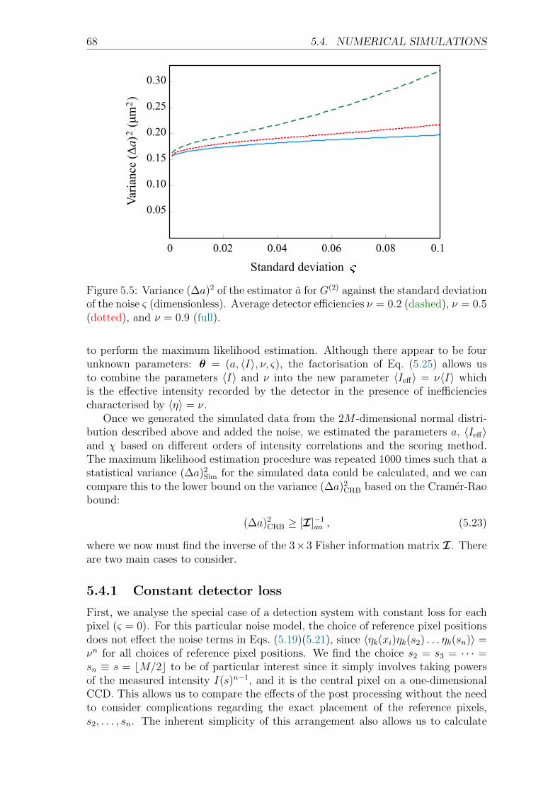
68 5.4. NUMERICAL SIMULATIONS
0 0.02 0.04 0.06 0.08 0.1
0.30
0.25
0.20
0.15
0.10
0.05
Standard deviation σ
Varia
nce
(Δa)
(μ
m )
22
Figure 5.5: Variance (∆a)2 of the estimator a for G(2) against the standard deviationof the noise ς (dimensionless). Average detector efficiencies ν = 0.2 (dashed), ν = 0.5(dotted), and ν = 0.9 (full).
to perform the maximum likelihood estimation. Although there appear to be fourunknown parameters: θ = (a, 〈I〉, ν, ς), the factorisation of Eq. (5.25) allows usto combine the parameters 〈I〉 and ν into the new parameter 〈Ieff〉 = ν〈I〉 whichis the effective intensity recorded by the detector in the presence of inefficienciescharacterised by 〈η〉 = ν.
Once we generated the simulated data from the 2M -dimensional normal distri-bution described above and added the noise, we estimated the parameters a, 〈Ieff〉and χ based on different orders of intensity correlations and the scoring method.The maximum likelihood estimation procedure was repeated 1000 times such that astatistical variance (∆a)2
Sim for the simulated data could be calculated, and we cancompare this to the lower bound on the variance (∆a)2
CRB based on the Cramer-Raobound:
(∆a)2CRB ≥ [I]−1
aa , (5.23)
where we now must find the inverse of the 3×3 Fisher information matrix I. Thereare two main cases to consider.
5.4.1 Constant detector loss
First, we analyse the special case of a detection system with constant loss for eachpixel (ς = 0). For this particular noise model, the choice of reference pixel positionsdoes not effect the noise terms in Eqs. (5.19)(5.21), since 〈ηk(xi)ηk(s2) . . . ηk(sn)〉 =νn for all choices of reference pixel positions. We find the choice s2 = s3 = · · · =sn ≡ s = bM/2c to be of particular interest since it simply involves taking powersof the measured intensity I(s)n−1, and it is the central pixel on a one-dimensionalCCD. This allows us to compare the effects of the post processing without the needto consider complications regarding the exact placement of the reference pixels,s2, . . . , sn. The inherent simplicity of this arrangement also allows us to calculate

CHAPTER 5. ESTIMATION OF THERMAL SOURCE DIMENSIONS 69
the correlations up to arbitrary order since the correlation functions G(n) and G(2n)
take the compact forms
G(n)(xi, s, . . . , s) =(n− 1)![1 + (n− 1)|γ(xi, s)|2],
G(2n)(xi, xj, s, . . . , s) =(n− 2)!
1 + |γ(xi, xj)|2 + (n− 2)
×[2Re(γ(xi, xj)γ(s, xi)γ(xj, s))
+ |γ(xi, s)|2 + |γ(xj, s)|2
+ |γ(xi, s)|2|γ(xj, s)|2]. (5.24)
Fig. 5.4c shows the Cramer-Rao lower bound on the variance for our estimate of a forthe first four correlation functions G(2) to G(5), and Fig. 5.4d shows the estimate ofa with the actual standard deviation ∆aSim. The numerical results are also collatedin Table 5.2.
Table 5.2: Results of the maximum likelihood estimation for the correlation functionsG(2) to G(5) and the Cramer-Rao lower bounds. The estimation procedure wasperformed on 1000 simulated data sets.
n Estimated a (µm) (∆a)2Sim (µm2) (∆a)2
CRB (µm2)
2 99.978 0.181 0.1623 99.968 0.151 0.1504 99.932 0.249 0.2445 99.826 0.543 0.434
Surprisingly, the best estimates of the spatial dimensions of the source occurfor n = 3, and the estimates get progressively worse as the correlation order isincreased beyond third order. Therefore, to extract the maximum amount of spatialinformation from our data, correlations of third order should be used. We stressthe importance of this finding as it requires no additional measurements to be madeother than those made to measure G(2). Indeed, in principle it would be possibleto use the exact data used by Hanbury Brown and Twiss to measure the angulardiameter of Sirius [Brown and Twiss, 1956a]. We also note that there is nothing inour treatment that uniquely picks out the spatial correlation functions, in the samemanner we could equally discuss temporal correlations. Interestingly, estimates ofthe effective intensity 〈Ieff〉 do not follow the same pattern as those for a. If wewish to estimate 〈Ieff〉 the best performance is given by G(2), with higher ordersperforming worse.
5.4.2 Detector loss as a random variable
Second, we demonstrate the effect of a small non-zero ς, representing a system withuncertainty in the detector loss mechanism. The effect of this additional noise isshown in Fig. 5.5, where we plot the variance of the estimator for the second orderintensity correlation function against the standard deviation ς. As expected, theaddition of noise in the detection process reduces the precision in our estimator, butthe question is whether this detector noise as a random variable is a better modelthan the fixed detector efficiency with ς = 0. The results of the maximum likelihoodestimation and the Cramer-Rao bound are given in Table 5.3.
70 5.4. NUMERICAL SIMULATIONS
In order to perform the estimation, first we must evaluate the second term inEq. (5.19), which is an nth moment of the noise distribution. Having considered thecase where all reference pixels are the same in the previous section, we now restrictourselves to only considering cases where no two reference pixel positions are thesame, i.e. s2 6= s3 6= · · · 6= sn, such that we can determine the effect of separat-ing the reference pixels. In this regime the nth moment of the noise distribution,〈η(xi)η(s2) . . . η(sn)〉 is given by
〈ηk(xi)ηk(s2) . . . ηk(sn)〉 = νn + νn−2
n∑
j=2
δxi,sj ς2
= νn
(1 +
n∑
j=2
δxi,sjχ2
)(5.25)
where χ = ς/ν. We therefore find it necessary to re-parameterise the problemusing the parameters θ = (a, 〈I〉, ν, χ). Eq. (5.25) represents an nth moment ofthe noise distribution, and the Kronecker deltas arise from the independence ofthe distribution for individual pixels. The 2nth moment of the noise distributionappearing in Eq. (5.21) is calculated in appendix B.
In order to find the optimum position of the reference pixels, we define |si−si+1| =d and plot the standard deviation as a function of d, the separation between adjacentreference pixels. Fig. 5.6 shows the standard deviation for G(2) to G(4) as a functionof d. Interestingly, the higher order correlations do not outperform G(2) for all valuesof d. For G(3) we find that the optimum positions correspond to separations wherethe two reference pixels become uncorrelated. This occurs whenever the complexdegree of coherence between the two pixels is equal to zero. Since the complexdegree of coherence for the system is proportional to the Bessel function J1, theoptimum separations d correspond to the zeroes of this function. For G(4) the exactposition of the optimum is more complicated, due to the fact that the zeroes of J1
are not uniformly distributed. However, the optimum positions are approximatelylocated at the position where adjacent reference pixels are uncorrelated from theirnearest neighbours. This should be expected to some extent as we can see from thefollowing argument: A measurement of G(3)(x, s1, s2) contains information aboutthe correlations between the fields at x and s1, and the fields at x and s2, thereforeif the fields at s1 and s2 are highly correlated we would expect to gain very littlefrom obtaining additional information regarding the correlations between x ands2. However, the more independent s1 and s2 become the more we can expect togain additional information from measurements of the correlations between x ands2. Tab. 5.3 shows the variance of the estimators for the first three correlationfunctions as calculated from the CRB and directly measured in the simulations. Wesee that the measured variance in our estimators closely follows that obtained fromthe CRB.
Another interesting feature of Fig. 5.6 is the ability for G(4) to outperform G(2), afeature that does not occur for fixed reference pixels. This behaviour is reminiscentof the “magic angles” in Refs. [Thiel et al., 2007, Oppel et al., 2012], where thedetectors had to be placed at specific positions (the magic angles) in order to obtainthe (n− 1)-fold increased sinusoidal modulation in the scanning detector.
The exact relation between the variance of our estimators and the correlationorder also depends on the intensity distribution of the source. Fig. 5.7 shows the
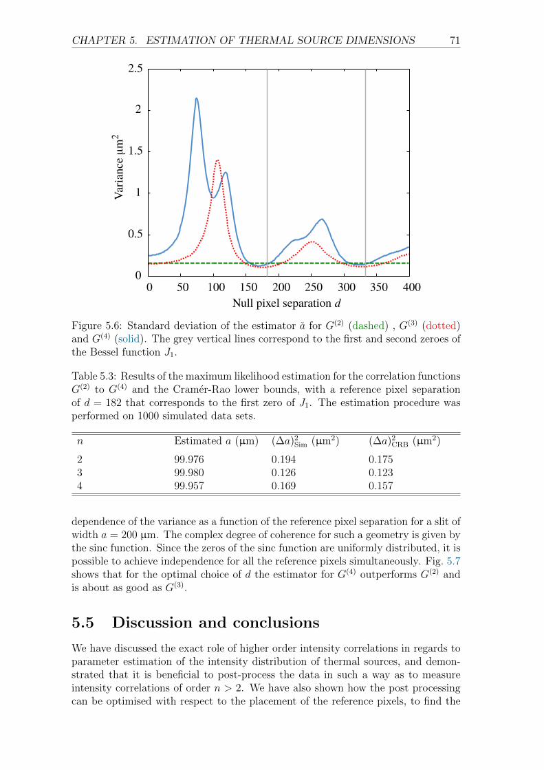
CHAPTER 5. ESTIMATION OF THERMAL SOURCE DIMENSIONS 71 7
0 50 100 150 200 250 300 350 4000
0.5
1
1.5
2
2.5
Varia
nceµ
m2
Null pixel separation d
FIG. 6: (Color online): Standard deviation of the estimator a forG(2) (dashed) , G(3) (dotted) and G(4) (solid). The grey vertical linescorrespond to the first and second zeroes of the Bessel function J1.
dard deviation n . As expected, the addition of noise in thedetection process reduces the precision in our estimator. Asmentioned in the previous section, the estimation procedurecannot proceed if we make the same choice of null pixel posi-tions, i.e. s2 = s3 = · · · = sn s. In order to find the optimumposition of the null pixels, we define |sisi+1 | = d and plot thestandard deviation as a function of d, the separation betweenadjacent null pixels. Fig. 6 shows the standard deviation forG(2)-G(4) as a function of d. Interestingly, the higher ordercorrelations do not outperform G(2) for all values of d. ForG(3) we find that the optimum positions correspond to sepa-rations where the two null pixels become uncorrelated. Thisoccurs whenever the complex degree of coherence betweenthe two pixels is equal to zero. Since the complex degree ofcoherence for the system is proportional to the Bessel func-tion J1, the optimum separations d correspond to the zeroesof this function. For G(4) the exact position of the optimumis more complicated, due to the fact that the zeroes of J1 arenot uniformly distributed. However, the optimum positionsare approximately located at the position where adjacent nullpixels are uncorrelated from their nearest neighbours.
Another interesting feature of Fig. 6 is the ability for G(4)
to outperform G(2), a feature that does not occur for s2 =s3 = · · · = sn . Tab. III shows the variance of the estimatorsfor the first three correlation functions as calculated from theCRB and directly measured in the simulations. We see thatthe measured variance in our estimators closely follows thatobtained from the CRB.
The exact relation between the variance of our estimatorsand the correlation order also depends on the intensity dis-tribution of the source. Fig. 7 shows the dependence of thevariance as a function of the null pixel separation for a slitof width a = 200 µm. The complex degree of coherence forsuch a geometry is given by the sinc function. Since the zerosof the sinc function are uniformly distributed, it is possibleto achieve independence for all the null pixels simultaneously.
Varia
nceµ
m2
Null pixel separation d0 50 100 150 200 250 300 350 400
0
1
2
3
4
5
6
7
FIG. 7: (Color online): Standard deviation of the estimator a forG(2) (dashed) , G(3) (dotted) and G(4) (solid). The grey vertical linescorrespond to the first and second zeroes of the sinc function.
The plot shows that for the right choice of d the estimator forG(4) outperforms G(2) and is almost as good as G(3) .
VI. DISCUSSION & CONCLUSIONS
The ability for higher order correlations to obtain more in-formation can often be a source of confusion. This is mostclearly demonstrated when the detector noise vanishes n = 0and the null pixels are all the same s2 = s3 = · · · = sn . Aspointed out above in reference to the original HBT experiment,we can take the output of two photodetectors and simply bytaking powers of one of the outputs, we gain a more preciseestimate of angular diameter of the source. We can understandthis increase in precision by comparing the measurements ofthe intensity and second order correlation function. We usethe same set of data when measuring the intensity as we use tomeasure the second order intensity correlation and yet a mea-surement of the intensity reveals very little information aboutthe source since the intensity of a thermal source in the farfield is constant across x, the position of the detector. In con-trast, the second order intensity correlation function is highlydependent on x which allows for a much more precise esti-mate of the angular diameter to be achieved, see Fig. 3. When
TABLE III: Variance of the estimators for the correlation functionsG(2)-G(4) calculated for null pixel separation d = 182 which cor-responds to the first zero of J1. The estimation procedure was per-formed on 1000 simulated data sets and the variance of the estimateswas calculated from the results.
n a (µm) (a)2Sim (µm2) (a)2
CRB (µm2)
2 99.976 0.194 0.1753 99.980 0.126 0.1234 99.957 0.169 0.157
Figure 5.6: Standard deviation of the estimator a for G(2) (dashed) , G(3) (dotted)and G(4) (solid). The grey vertical lines correspond to the first and second zeroes ofthe Bessel function J1.
Table 5.3: Results of the maximum likelihood estimation for the correlation functionsG(2) to G(4) and the Cramer-Rao lower bounds, with a reference pixel separationof d = 182 that corresponds to the first zero of J1. The estimation procedure wasperformed on 1000 simulated data sets.
n Estimated a (µm) (∆a)2Sim (µm2) (∆a)2
CRB (µm2)
2 99.976 0.194 0.1753 99.980 0.126 0.1234 99.957 0.169 0.157
dependence of the variance as a function of the reference pixel separation for a slit ofwidth a = 200 µm. The complex degree of coherence for such a geometry is given bythe sinc function. Since the zeros of the sinc function are uniformly distributed, it ispossible to achieve independence for all the reference pixels simultaneously. Fig. 5.7shows that for the optimal choice of d the estimator for G(4) outperforms G(2) andis about as good as G(3).
5.5 Discussion and conclusions
We have discussed the exact role of higher order intensity correlations in regards toparameter estimation of the intensity distribution of thermal sources, and demon-strated that it is beneficial to post-process the data in such a way as to measureintensity correlations of order n > 2. We have also shown how the post processingcan be optimised with respect to the placement of the reference pixels, to find the
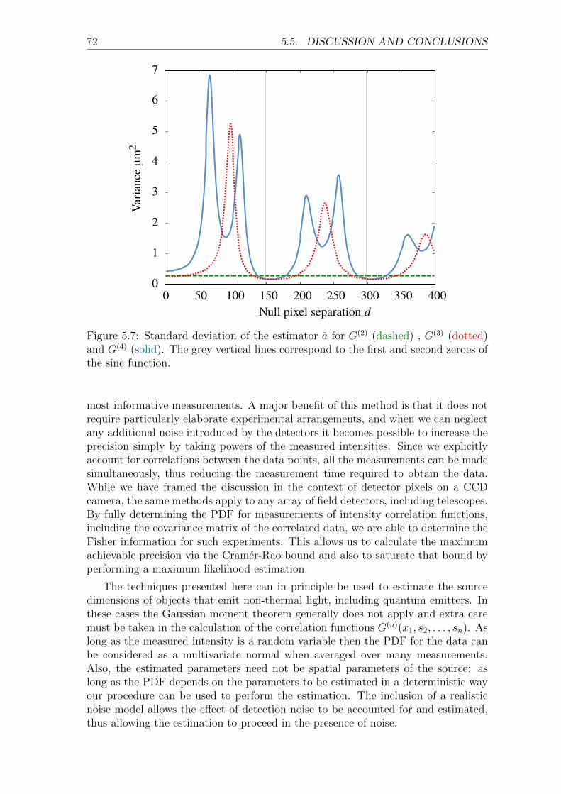
72 5.5. DISCUSSION AND CONCLUSIONS7
0 50 100 150 200 250 300 350 4000
0.5
1
1.5
2
2.5
Varia
nceµ
m2
Null pixel separation d
FIG. 6: (Color online): Standard deviation of the estimator a forG(2) (dashed) , G(3) (dotted) and G(4) (solid). The grey vertical linescorrespond to the first and second zeroes of the Bessel function J1.
dard deviation n . As expected, the addition of noise in thedetection process reduces the precision in our estimator. Asmentioned in the previous section, the estimation procedurecannot proceed if we make the same choice of null pixel posi-tions, i.e. s2 = s3 = · · · = sn s. In order to find the optimumposition of the null pixels, we define |sisi+1 | = d and plot thestandard deviation as a function of d, the separation betweenadjacent null pixels. Fig. 6 shows the standard deviation forG(2)-G(4) as a function of d. Interestingly, the higher ordercorrelations do not outperform G(2) for all values of d. ForG(3) we find that the optimum positions correspond to sepa-rations where the two null pixels become uncorrelated. Thisoccurs whenever the complex degree of coherence betweenthe two pixels is equal to zero. Since the complex degree ofcoherence for the system is proportional to the Bessel func-tion J1, the optimum separations d correspond to the zeroesof this function. For G(4) the exact position of the optimumis more complicated, due to the fact that the zeroes of J1 arenot uniformly distributed. However, the optimum positionsare approximately located at the position where adjacent nullpixels are uncorrelated from their nearest neighbours.
Another interesting feature of Fig. 6 is the ability for G(4)
to outperform G(2), a feature that does not occur for s2 =s3 = · · · = sn . Tab. III shows the variance of the estimatorsfor the first three correlation functions as calculated from theCRB and directly measured in the simulations. We see thatthe measured variance in our estimators closely follows thatobtained from the CRB.
The exact relation between the variance of our estimatorsand the correlation order also depends on the intensity dis-tribution of the source. Fig. 7 shows the dependence of thevariance as a function of the null pixel separation for a slitof width a = 200 µm. The complex degree of coherence forsuch a geometry is given by the sinc function. Since the zerosof the sinc function are uniformly distributed, it is possibleto achieve independence for all the null pixels simultaneously.
Varia
nceµ
m2
Null pixel separation d0 50 100 150 200 250 300 350 400
0
1
2
3
4
5
6
7
FIG. 7: (Color online): Standard deviation of the estimator a forG(2) (dashed) , G(3) (dotted) and G(4) (solid). The grey vertical linescorrespond to the first and second zeroes of the sinc function.
The plot shows that for the right choice of d the estimator forG(4) outperforms G(2) and is almost as good as G(3) .
VI. DISCUSSION & CONCLUSIONS
The ability for higher order correlations to obtain more in-formation can often be a source of confusion. This is mostclearly demonstrated when the detector noise vanishes n = 0and the null pixels are all the same s2 = s3 = · · · = sn . Aspointed out above in reference to the original HBT experiment,we can take the output of two photodetectors and simply bytaking powers of one of the outputs, we gain a more preciseestimate of angular diameter of the source. We can understandthis increase in precision by comparing the measurements ofthe intensity and second order correlation function. We usethe same set of data when measuring the intensity as we use tomeasure the second order intensity correlation and yet a mea-surement of the intensity reveals very little information aboutthe source since the intensity of a thermal source in the farfield is constant across x, the position of the detector. In con-trast, the second order intensity correlation function is highlydependent on x which allows for a much more precise esti-mate of the angular diameter to be achieved, see Fig. 3. When
TABLE III: Variance of the estimators for the correlation functionsG(2)-G(4) calculated for null pixel separation d = 182 which cor-responds to the first zero of J1. The estimation procedure was per-formed on 1000 simulated data sets and the variance of the estimateswas calculated from the results.
n a (µm) (a)2Sim (µm2) (a)2
CRB (µm2)
2 99.976 0.194 0.1753 99.980 0.126 0.1234 99.957 0.169 0.157
Figure 5.7: Standard deviation of the estimator a for G(2) (dashed) , G(3) (dotted)and G(4) (solid). The grey vertical lines correspond to the first and second zeroes ofthe sinc function.
most informative measurements. A major benefit of this method is that it does notrequire particularly elaborate experimental arrangements, and when we can neglectany additional noise introduced by the detectors it becomes possible to increase theprecision simply by taking powers of the measured intensities. Since we explicitlyaccount for correlations between the data points, all the measurements can be madesimultaneously, thus reducing the measurement time required to obtain the data.While we have framed the discussion in the context of detector pixels on a CCDcamera, the same methods apply to any array of field detectors, including telescopes.By fully determining the PDF for measurements of intensity correlation functions,including the covariance matrix of the correlated data, we are able to determine theFisher information for such experiments. This allows us to calculate the maximumachievable precision via the Cramer-Rao bound and also to saturate that bound byperforming a maximum likelihood estimation.
The techniques presented here can in principle be used to estimate the sourcedimensions of objects that emit non-thermal light, including quantum emitters. Inthese cases the Gaussian moment theorem generally does not apply and extra caremust be taken in the calculation of the correlation functions G(n)(x1, s2, . . . , sn). Aslong as the measured intensity is a random variable then the PDF for the data canbe considered as a multivariate normal when averaged over many measurements.Also, the estimated parameters need not be spatial parameters of the source: aslong as the PDF depends on the parameters to be estimated in a deterministic wayour procedure can be used to perform the estimation. The inclusion of a realisticnoise model allows the effect of detection noise to be accounted for and estimated,thus allowing the estimation to proceed in the presence of noise.
CHAPTER 5. ESTIMATION OF THERMAL SOURCE DIMENSIONS 73
The experimental implementation of this procedure is not hugely challenging,but a number of critical requirements must be met. First, when measuring theintensity correlation functions, the integration time of the detectors must be wellbelow the coherence time of the radiation to ensure that each measurement capturesa single mode of the radiation allowing us to consider a single mode. In addition,the area of each detector (pixel) must be much smaller than the coherence area ofthe source such that a single pixel can be considered as measuring a single mode.This ensures that every detection event samples no more than a single mode volume(i.e., the speckle size). Second, our use of the central limit theorem implies thatwe have a large data set that provides a good signal to noise ratio. It is well-known that a maximum likelihood estimation procedure requires a good signal tonoise ratio to produce good estimates [Kay, 1993]. Third, we have assumed uniformintensity across the detectors. In practice this can be challenging if the source is notsufficiently out of focus, or if there are spurious interference effects in the detectoritself (e.g., an etalon effect due to the protective glass of a CCD camera). Finally, thedetector noise is uncorrelated, which means that the pixel efficiencies are random,and there is no cross-talk between the pixels. The latter two requirements can inprinciple be included in the modelling of the experiment, but this comes at the costof a significantly increased complexity of the correlation functions.
We notice from Fig. (5.4) that all of the estimates fall just below the actualvalue of a = 100 µm. Since all estimates are within one standard deviation of thetrue value this may well be due to statistical fluctuations but it is also possible thatthere is a small bias in the estimator. Presumably this would be due to any slightdeviations away from a normal distribution as was assumed for the PDF for thedata. To model the PDF as a multivariate normal requires the use of the centrallimit theorem, which is only strictly true in the limit of infinite averaging. If thereis in fact a bias and it is caused by the non-normal nature of the PDF, we wouldexpect this effect to disappear for larger data sets as the PDF approaches normality.
The ability for higher order correlations to obtain more information can often bea source of confusion. This is most clearly demonstrated when the reference pixelsare all the same s2 = s3 = · · · = sn. We can take the output of two photodetectorsand simply by taking powers of one of the outputs, we gain a more precise estimateof angular diameter of the source. We can understand this increase in precision bycomparing the measurements of the intensity and second order correlation functionas in the original HBT experiment. We use the same set of data when measuringthe intensity as we use to measure the second order intensity correlation and yet ameasurement of the intensity reveals very little information about the source sincethe intensity of a thermal source in the far field is constant across x, the position ofthe detector. In contrast, the second order intensity correlation function is highlydependent on x which allows for a much more precise estimate of the angular di-ameter to be achieved, see Fig. 5.3. When considered as another method of postprocessing the data, it is no more surprising that higher order correlations outper-form the second order correlation than the second order correlation outperformingthe intensity.
Our method is rather general, and should apply to sources of light that are notthermal. Future work will focus on (multi-mode) squeezed light and single photonsources. Since all correlation functions can be determined from the same data set, itwould be advantageous to combine all of the estimates achieved via different n into a

74 5.5. DISCUSSION AND CONCLUSIONS
single estimate. In order to do this properly we would need to know exactly how allof the individual estimates are correlated to determine the appropriate weighting forthe combined estimate and its error. The difficulty in determining the correlation isin knowing how the maximum likelihood estimation procedure affects the correlation,if at all. Once this is known, it should be possible to determine the weighting andobtain the final estimate.
In conclusion, we found that higher order correlation functions can substantiallyimprove estimation of the parameters that characterise the geometry of a thermallight source. As long as the source and the detection system are properly modelled,the procedure can be implemented with current technology. Our techniques extendimmediately to other forms of Gaussian light, and potentially more general classicaland quantum light sources as well.
Chapter 6
Obtaining Spatial InformationFrom Far Field Sources
We often wish to determine the spatial properties of a radiation source from mea-surements of the radiation in the far field. There are numerous measurements wecan make to aid us in determining these spatial properties. In this chapter we focuson the problem of determining the spatial properties of a source of thermal radia-tion from measurements of the radiation in the far field although our method onlyrelies on the detected radiation being diagonal in the number basis and isotropic (atleast across the modes that are measured). We calculate the symmetric logarithmicderivative for such a system and determine under what circumstances the expres-sions lead to a well behaved quantum Fisher information matrix. We also determineunder what circumstances the quantum Fisher information (QFI) is ill-defined andin fact becomes singular. This allows us to demonstrate certain physical restrictionsupon the measured radiation and therefore informs us as to how information aboutthe spatial distribution of a source is conveyed to the far field.
At the end of this chapter we examine how, using the method developed here,we might come to obtain a complete calculation of the quantum Fisher information.We also give a brief account of an entirely different approach that may lead to asuccessful calculation of the QFI and point out what difficulties we anticipate toencounter.
6.1 Blackbody radiation
We start by discussing the properties of blackbody radiation. It is well known thatblackbody radiation is described by the density operator [Mandel and Wolf, 1995]
ρ =⊗
k,s
∞∑
nks=0
〈nks〉nks
(1 + 〈nks〉)nks+1|nks〉〈nks| (6.1)
≡⊗
k,s
∞∑
nks=0
p(nks)|nks〉〈nks|, (6.2)
where the product⊗
k,s labels all of the occupied modes, k labels the wave vectorand s labels the polarisation. The product should be understood as a tensor product
75

76 6.1. BLACKBODY RADIATION
Figure 6.1: The Planck distribution describing the energy spectrum of the radia-tion emitted by a blackbody. The peak of the distribution is proportional to thetemperature of the blackbody T and can be determined via Wien’s displacementlaw.
over the individual density operators describing each mode
ρks =∑
nks
p(nks)|nks〉〈nks|
ρ =⊗
k,s
ρks, (6.3)
which therefore describe independent states of the field. We can consider the productas split into two parts
⊗k =
⊗k
⊗[k] where the first product is taken over wavevec-
tors of different magnitude and the second product is constrained to wavevectorsof magnitude k but specifying unique directions. By noticing that the magnitudeof the wave vector is proportional to the frequency ν we can write the product as⊗
ν
⊗[k].
A blackbody emits isotropically in space meaning that all k modes are occupiedand the energy of the state follows a Planck distribution in frequency (see Fig. 6.1)
B(ν) =2hν3
c2
1
eβhν − 1, (6.4)
where h is the Planck constant, β = 1/kBT and kB is the Boltzmann constant. ThePlanck distribution gives the amount of energy emitted by a blackbody per unittime, per steradian, per Hertz, per square meter of the source, Wsr−1Hz−1m−21. Tocalculate the actual energy output of a blackbody of area AS, over a frequency range
1A steradian is defined in analogous way to the radian in 3 dimensions. As the definition ofthe radian is the angle subtended at the centre of a circle by an arc that has length equal to theradius of the circle, the steradian is the solid angle subtended at the centre of a sphere by a conethat encompasses an area of the radius squared over the surface of the sphere.
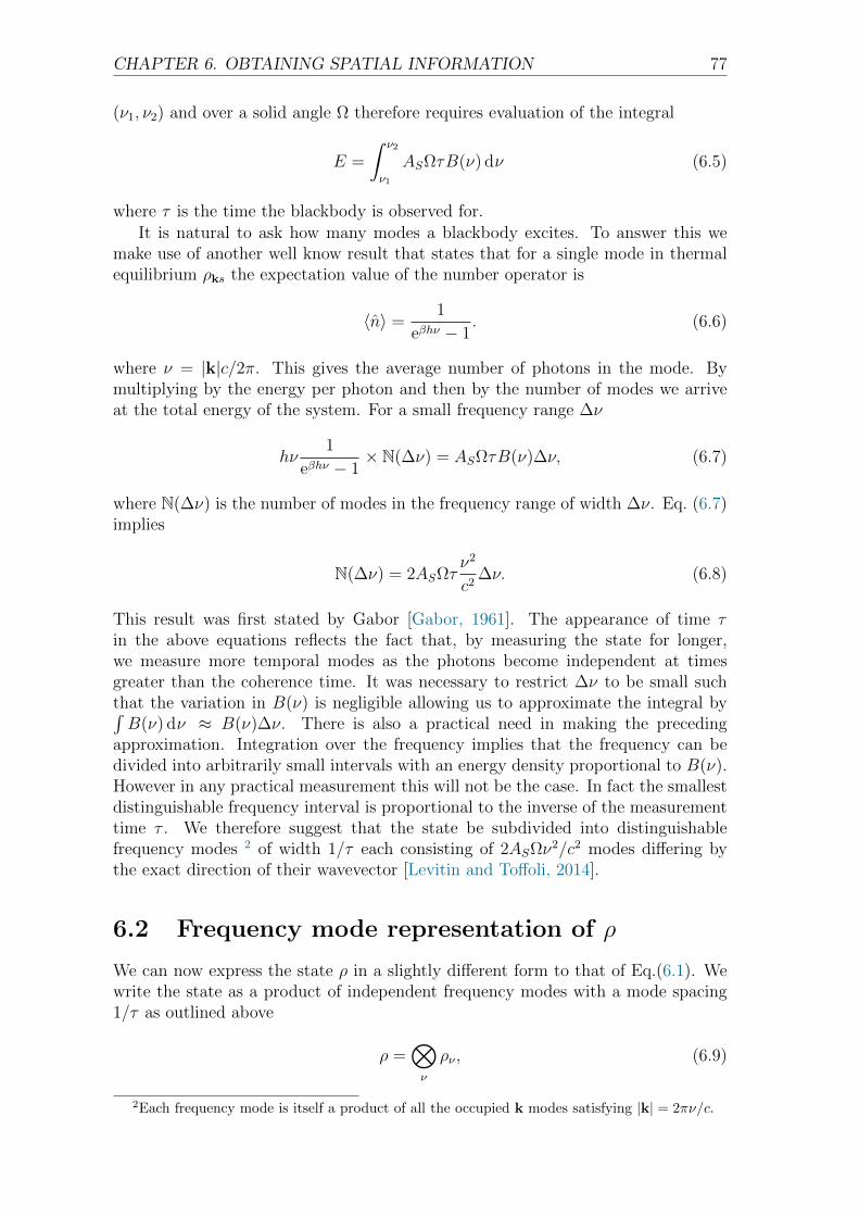
CHAPTER 6. OBTAINING SPATIAL INFORMATION 77
(ν1, ν2) and over a solid angle Ω therefore requires evaluation of the integral
E =
∫ ν2
ν1
ASΩτB(ν) dν (6.5)
where τ is the time the blackbody is observed for.It is natural to ask how many modes a blackbody excites. To answer this we
make use of another well know result that states that for a single mode in thermalequilibrium ρks the expectation value of the number operator is
〈n〉 =1
eβhν − 1. (6.6)
where ν = |k|c/2π. This gives the average number of photons in the mode. Bymultiplying by the energy per photon and then by the number of modes we arriveat the total energy of the system. For a small frequency range ∆ν
hν1
eβhν − 1× N(∆ν) = ASΩτB(ν)∆ν, (6.7)
where N(∆ν) is the number of modes in the frequency range of width ∆ν. Eq. (6.7)implies
N(∆ν) = 2ASΩτν2
c2∆ν. (6.8)
This result was first stated by Gabor [Gabor, 1961]. The appearance of time τin the above equations reflects the fact that, by measuring the state for longer,we measure more temporal modes as the photons become independent at timesgreater than the coherence time. It was necessary to restrict ∆ν to be small suchthat the variation in B(ν) is negligible allowing us to approximate the integral by∫B(ν) dν ≈ B(ν)∆ν. There is also a practical need in making the preceding
approximation. Integration over the frequency implies that the frequency can bedivided into arbitrarily small intervals with an energy density proportional to B(ν).However in any practical measurement this will not be the case. In fact the smallestdistinguishable frequency interval is proportional to the inverse of the measurementtime τ . We therefore suggest that the state be subdivided into distinguishablefrequency modes 2 of width 1/τ each consisting of 2ASΩν2/c2 modes differing bythe exact direction of their wavevector [Levitin and Toffoli, 2014].
6.2 Frequency mode representation of ρ
We can now express the state ρ in a slightly different form to that of Eq.(6.1). Wewrite the state as a product of independent frequency modes with a mode spacing1/τ as outlined above
ρ =⊗
ν
ρν , (6.9)
2Each frequency mode is itself a product of all the occupied k modes satisfying |k| = 2πν/c.
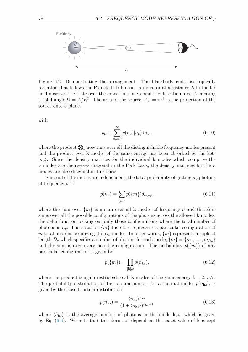
78 6.2. FREQUENCY MODE REPRESENTATION OF ρ
Figure 6.2: Demonstrating the arrangement. The blackbody emits isotropicallyradiation that follows the Planck distribution. A detector at a distance R in the farfield observes the state over the detection time τ and the detection area A creatinga solid angle Ω = A/R2. The area of the source, AS = πr2 is the projection of thesource onto a plane.
with
ρν ≡∞∑
nν=0
p(nν)|nν〉〈nν |, (6.10)
where the product⊗
ν now runs over all the distinguishable frequency modes presentand the product over k modes of the same energy has been absorbed by the kets|nν〉. Since the density matrices for the individual k modes which comprise theν modes are themselves diagonal in the Fock basis, the density matrices for the νmodes are also diagonal in this basis.
Since all of the modes are independent, the total probability of getting nν photonsof frequency ν is
p(nν) =∑
mp(m)δm,nν , (6.11)
where the sum over m is a sum over all k modes of frequency ν and thereforesums over all the possible configurations of the photons across the allowed k modes,the delta function picking out only those configurations where the total number ofphotons is nν . The notation m therefore represents a particular configuration ofm total photons occupying the Dν modes. In other words, m represents a tuple oflength Dν which specifies a number of photons for each mode, m = m1, . . . ,mDνand the sum is over every possible configuration. The probability p(m) of anyparticular configuration is given by
p(m) =∏
[k],s
p(nks), (6.12)
where the product is again restricted to all k modes of the same energy k = 2πν/c.The probability distribution of the photon number for a thermal mode, p(nks), isgiven by the Bose-Einstein distribution
p(nks) =〈nks〉nks
(1 + 〈nks〉)nks+1(6.13)
where 〈nks〉 is the average number of photons in the mode k, s, which is givenby Eq. (6.6). We note that this does not depend on the exact value of k except
CHAPTER 6. OBTAINING SPATIAL INFORMATION 79
through its absolute value |k| = k, we therefore find that each term in the productof Eq. (6.12) gives the same contribution allowing us to write
p(m) = p(nks)Dν , (6.14)
where we have defined Dν to be the number of k modes at frequency ν.Substituting from Eq. (6.13) into Eq. (6.14), we find
p(m) =〈nks〉nν
(1 + 〈nks〉)nν+Dν, (6.15)
where nν ≡ Dνnks. As this depends only upon the total number of photons nνand not upon the actual configuration, each term that contributes to the sum inEq. (6.11) gives the same result, namely Eq. (6.14). The probability p(nν) is there-fore given by Np(m) where N is the number of ways of arranging nν photonsacross Dν modes. We find
p(nν) =(nν +Dν − 1)!
(Dν − 1)!nν !
〈nks〉nν(1 + 〈nks〉)nν+Dν
, (6.16)
which is the probability of measuring nν photons of frequency ν given that there areDν unique k modes in which the photons are distributed where each mode has thesame average occupation number 〈nks〉 [Mandel, 1959]. The number of k modes ofa source of area AS viewed under a solid angle Ω is equal to [Levitin and Toffoli,2014]
Dν = 2ASΩν2
c2. (6.17)
The factor of 2 in the above equation accounts for polarisation allowing us to omits from the following treatment to simplify notation. In going from Eq. (6.8) wehave cancelled the factor ∆ν with the 1/τ . In doing so we insist that whatever timeinterval the state is measured over inversely defines the frequency interval ∆ν, whichensures that whatever time interval is chosen, only one temporal mode is measured.
6.3 The quantum Fisher information for black-
body radiation
To calculate the QFI for the spatial parameters of the source, we need to take thederivative of ρ with respect to the parameters θ = θ1, . . . , θr, which parameterisethe spatial properties of the source. The QFI matrix is given by [Helstrom, 1976]
[IQ]ij = Tr[(∂iρ)Lj], (6.18)
where Lj is the symmetric logarithmic derivative with respect to the parameter θjand ∂i ≡ ∂
∂θi.
Calculation of the QFI therefore relies upon calculating the symmetric logarith-mic derivative (SLD). In the basis that diagonalises ρ the SLD is given by
Lj = 2∑
l,m
〈l|∂jρ|m〉p(l) + p(m)
|l〉〈m| (6.19)

80 6.3 THE QUANTUM FISHER INFORMATION
where p(l) and |l〉 are the eigenvalues and eigenbasis of ρ respectively. In generalthe eigenvalues and eigenbasis of ρ will change with the parameters θ, thereforewhen we take the derivatives we must be careful to ensure that we take this intoaccount. However, we will avoid explicitly writing the θ dependence in both theeigenvalues and eigenbasis for brevity. Since each individual k mode that constitutesρ is diagonal in the number basis, ρ itself is diagonal in the basis |l〉 =
⊗k|lk〉,
where again the notation l stands for a tuple of length Dν denoting the the numberof photons in mode k. The matrix elements 〈l|∂jρ|k〉 are
[∂jρ]lk = 〈l|∑
ν
∂jρν⊗
µ6=νρµ|k〉
=∑
ν
〈lν |∂jρν |kν〉⊗
µ6=νp(lµ)δlµ,kµ . (6.20)
The SLD then becomes
Lj = 2∑
ν
∑
lν ,kν
〈lν |∂jρν |kν〉p(lν) + p(kν)
|lν〉〈kν |. (6.21)
Using this form for the SLD and Eq. (6.18), the QFI is
[IQ]ij =∑
ν
Tr
[2∂iρν
∑
lν ,kν
〈lν |∂jρν |kν〉p(lν) + p(kν)
|lν〉〈kν |]. (6.22)
The QFI is therefore the sum of the QFI for each mode, we will omit the mode labeland write the QFI for a single mode ν as
[IQ](ν)ij = Tr
[2∂iρ
∑
l,k
〈l|∂jρ|k〉pl + pk
|l〉〈k|]. (6.23)
Upon inserting Eq. (6.20) into Eq. (6.23) we find
[IQ](ν)ij = 2
∑
l,k
〈k|∂jρ|l〉〈l|∂iρ|k〉pl + pk
, (6.24)
where the QFI now depends only on the probabilities pl and the matrix elements〈l|∂iρ|k〉.
Evaluating first the matrix elements 〈k|∂iρ|k〉, we find
〈l|∂iρ|k〉 =∑
n
∂jpnδl,nδn,k + pn〈l| (∂j|n〉〈n|) |k〉, (6.25)
where we are careful to remember that the basis |n〉 is the basis that diagonalisesρ and is therefore dependent on θ. Remembering that the state |n〉 is defined by|n〉 =
⊗kν|nk〉 where the product is again constrained to wave vectors that satisfy
|k| = k = 2πνc, which we denote as kν . We are now faced with the issue that thenumber of k modes at a particular frequency ν, Dν , is dependent on the spatialproperties of the source. To proceed we calculate 〈lk| (∂i|nk〉〈nk|) |kk〉 and find thatit is not dependent on k except through the magnitude |k|, and hence we may write
〈l| (∂i|n〉〈n|) |k〉 = 〈lk|Dν(∂i|nk〉〈nk|Dν
)|kk〉Dν , (6.26)
CHAPTER 6. OBTAINING SPATIAL INFORMATION 81
where both Dν and |nk〉〈nk| depend on θj.Since θi is a spatial property of the source, we find it convenient to express |nk〉
in the spatial basis
|nk〉 =
∫
A
dx1 . . .
∫
A
dxn ψn(x1, . . . ,xn)|x1, . . . ,xn〉, (6.27)
where the limits on the integral are imposed by the area over which we detectthe state ρ, ψn(x1, . . . ,xn) is the spatial wavefunction of the n-photon Fock statein mode k and |x1, . . . ,xn〉 = n!−1a†(x1) . . . a†(xn)|0〉. We can relate the spatialcoordinates x1, . . . ,xn in the detection plane to the spatial coordinates y1, . . . ,ynin the source plane via the appropriate Green’s function, G(yi,xi). The n photonFock state then becomes
|nk〉 =1√n!N
∫
A
dnx
∫
S
dny φn(y1, . . . ,yn)
×G(y1,x1) . . . G(yn,xn)a†(y1) . . . a†(yn)|0〉, (6.28)
where√N is the normalisation factor and the subscript S denotes integration over
the source.Upon expanding 〈lk| (∂i|nk〉〈nk|) |kk〉, we find
〈lk| (∂i|nk〉〈nk|) |kk〉 = 〈lk|∂i|nk〉δn,k + (∂i〈nk|)|kk〉δl,n. (6.29)
Using Eq. (6.28) we see that the inner product 〈lk|∂i|nk〉 is proportional to an anti-normally ordered product of creation and annihilation operators
〈lk|∂i|nk〉 ∝ 〈0|a(y′1) . . . a(y′l)a†(y1) . . . a†(yn)|0〉
= δn,l∑
σ∈Sn
n∏
i=1
δ(yi − y′σ(i)), (6.30)
where Sn is the symmetric group containing all the permutations of the set 1, . . . , n.Since we integrate over all coordinates y1 . . .yn and y′1 . . .y
′n each of the terms in
the sum over Sn gives the same result after an arbitrary re-labelling of variables.Due to the Kronecker delta δn,l, we need only consider the term 〈nk|∂i|nk〉:
〈nk|∂i|nk〉 =1√N
∫
A
dnx′ ∂i
[1√N
∫
A
dnx
∫
S
dny |φn(y1, . . . ,yn)|2
×n∏
i=1
G∗(yi,x′i)G(yi,xi)
], (6.31)
where we have integrated over all n of the y′ coordinates, making use of the Diracdelta functions in Eq. (6.30).
The inner product now becomes
〈nk|∂i|nk〉 =1√N∂i
[ Jn√N
]. (6.32)
where we have defined
Jn =
∫
A
dnx′∫
A
dnx
∫
S
dny |φn(y1, . . . ,yn)|2G∗(yi,x′i)G(yi,xi). (6.33)
82 6.3 THE QUANTUM FISHER INFORMATION
Now, using the fact that the state |nk〉 is normalised, we can write 〈nk|nk〉 ≡ 1 =Jn/N , and therefore
〈nk|∂i|nk〉 =1
2∂i [ln(Jn)] (6.34)
The inner product (∂i〈nk|)|nk〉 in Eq. (6.25) gives the same result3. If the Green’sfunction is dependent on k only through the magnitude |k|, then the inner productdoes not depend on the exact k mode we are considering 4. Therefore, we can write
(∂i|nν〉〈nν |) =∂i|nk〉〈nk|Dν= (∂iDν) |nk〉〈nk|Dν ln(|nk〉〈nk|)
+Dν (∂i|nk〉〈nk|) |nk〉〈nk|Dν−1
=Dν (∂i|nk〉〈nk|) |nk〉〈nk|Dν−1, (6.35)
where we have used,
(∂iDν)|nk〉〈nk|Dν ln(|nk〉〈nk|) =
limx↑1
xDν ln(x) 0 . . .
0 (1− x)Dν ln(1− x) . . ....
.... . .
= 0, (6.36)
The QFI then becomes
[IQ](ν)ij =
∑
nν
p(nν) [∂i ln(p(nν)Jnν )] [∂j ln(p(nν)Jnν )] . (6.37)
We notice that the form of the QFI as given by Eq. (6.37) is manifestly symmetricin i, j. This is a well understood property if the quantum Fisher information matrixand has its roots in the fact that the QFI matrix is the metric in the probabilityspace of the parameters θ = (θ1, . . . , θr). Expanding the logarithms of Eq. (6.37)we find
[IQ](ν)ij =
∑
nν
p(nν)
[∂i ln(p(nν))] [∂j ln(p(nν))] + [∂i ln(Jnν )] [∂j ln(p(nν))]
+ [∂i ln(p(nν))] [∂j ln(Jnν )] + [∂i ln(Jnν )] [∂j ln(Jnν )]. (6.38)
The first term in Eq. (6.38) has a clear physical interpretation, it is the classicalFisher information associated with the probability distribution p(nν) and as suchdescribes the amount of information we can obtain by measuring the total numberof photons (or equivalently the total intensity) across the whole detector. Physi-cally we would expect that total photon number recorded by the detector would beproportional to the radiating area of the source, AS. Therefore, a radiating source
3Technically the inner product (∂i〈nk|)|nk〉 = (〈nk|∂i|nk〉)∗. However, since Jn is typically apositive, real quantity, we will ignore this technicality from now on, keeping in mind that we canuse α+ α∗ = 2 Reα later if we are required.
4This approximation is valid for far field paraxial observation where the Green’s function isapproximately given by (−ik/2πR)eik|y−x| [Mandel and Wolf, 1995].
CHAPTER 6. OBTAINING SPATIAL INFORMATION 83
parameterised by more than one parameter, e.g. a rectangular source of sides a andb, should present us with an over-defined problem due to the infinity of solutions tothe equation AS = ab. Using the definition of p(nν), Eq. (6.16) and the chain rulewe can write ∂ip(nν) = ∂ASp(nν)∂iAS and we therefore find
∑
nν
p(nν) [∂i ln(p(nν))] [∂j ln(p(nν))] =∑
nν
1
p(nν)[∂ip(nν)] [∂jp(nν)]
=∑
nν
1
p(nν)[∂ASp(nν)]
2[∂iAS][∂jAS]. (6.39)
The entire dependence on nν has now factored out of the derivatives which leads toa singular Fisher information matrix, which can be seen by writing the expressionout for two parameters,
P
(∂1AS∂1AS ∂1AS∂2AS∂2AS∂1AS ∂2AS∂2AS.
)(6.40)
where we have defined P =∑
nνp(nν)
−1[∂ASp(nν)]2. We see straight away that
this matrix is singular since the determinant is zero. Another way of observing thisresult is that the matrix previously defined can be written as the outer product ofthe vector (∂1AS, . . . , ∂rAS) with itself. The rank of a matrix formed by taking anouter product of two vectors is always equal to 1. Since this matrix is then rankdeficient, it must be singular. This establishes the fact that only a single parameter,namely the area of the source, can be estimated from measurements of the totalphoton number or intensity.
Now we consider the cross terms in Eq. (6.38). We can write
∑
nν
p(nν) [∂i ln(Jnν )] [∂j ln(p(nν))] =∑
nν
[∂i ln(Jnν )] [∂jp(nν)]
=∑
nν
[∂ASp(nν)] [∂i ln(Jnν )] [∂jAS] , (6.41)
and we again find that the matrix defined by this term is rank 1 and singular as itcan again be formed by a vector outer product. Similarly the matrix defined by theother cross term is also singular. The last term in Eq. (6.38) is the only term forwhich the n dependence does not generally factorise outside of the derivatives andtherefore it is the only term that, taken on its own, does not lead to a singular QFImatrix.
It is instructive to examine in detail under what conditions the last term inEq. (6.38) leads to a non-singular QFI matrix. We start our investigation by return-ing to Eq. (6.33), and in particular we examine the term |φn(y1, . . . ,yn)|2, whichis the spatial wavefunction of the n photon state. If we treat the n photons as in-dependent then we can write |φn(y1, . . . ,yn)|2 = |φ1(y1)|2 . . . |φ1(yn)|2, which leadsto
Jn =
∫
A
dnx′∫
A
dnx
∫
S
dnyn∏
i=1
|φ1(yi)|2G∗(yi,x′i)G(yi,xi). (6.42)

84 6.4. SPATIALLY SEPARATED SOURCES
Since all n x, x′ and y variables are integrated over the same area (A, A and Srespectively), we end up with n copies of the same integral, namely
Jn =
[∫
A
dx′∫
A
dx
∫
S
dy |φ1(y)|2G∗(y,x′)G(y,x)
]n
≡ J n1 . (6.43)
This ultimately leads to
∑
nν
p(nν)n2ν [∂i ln(J1)] [∂j ln(J1)] , (6.44)
which again leads to a singular QFI matrix when taken on its own. Since the QFImatrix is then the sum of four singular, rank 1 matrices, the QFI matrix itself maybe non-singular. Due to the sub-additivity of the matrix rank, we can be sure thatthe QFI will be singular when its dimension is greater than four. However, we canbe more precise. Writing the QFI as
[IQ](ν)ij =
∑
nν
p(nν)[X2nνYiYj + nνXnνZiYj + nνXnνYiZj + n2
νZiZj], (6.45)
where Xnν = ∂ASp(nν), Yi = ∂iAS and Zi = ∂i ln(J1), we find that rank([IQ](ν)) = 2.The maximum dimension of the QFI matrix, and therefore the number of parameterswe can estimate, is two. Any attempt to estimate more than two parameters willlead to a rank two QFI matrix of dimension > 2, which means that the matrix will berank deficient and therefore not invertible. Clearly this does not describe a generalparameter estimation problem and the limit to the number of parameters suggeststhat when we treat the photons as statistically independent entities, we cannotperform the most general parameter estimation on the system. This reflects thattruly independent photons will remain independent even after propagation, thereforemeasurements of the photon correlations cannot be used to determine the spatialproperties of the source as in HBT measurements. We therefore conclude that the n-photon wavefunction |φn(y1, . . . ,yn)|2 cannot simply factorise meaning the photonscannot be independent. Physically we should expect that the wavefunction shouldnot factorise since we integrate over all y variables and therefore when two or morey variables are close together, within the coherence area of the source, the photonswill certainly be correlated. This indicates that the origin of the spatial informationof the source in the far field is the result of correlations that exist in the photons atthe source.
6.4 Spatially separated sources
In the previous section we witnessed that the factorisation of the multi-photon wave-function |φn(y1, . . . ,yn)|2 leads to a singular QFI matrix. Factorisation of the wave-function implies independence of the photons. However, it is known from the workof Oppel et al. [Oppel et al., 2012] that independent photons can be used to esti-mate the distribution of independent sources. These two results appear to be indisagreement. However, upon examining the problem more closely we find that nosuch disagreement exists. We take as an example two spatially separated sources S1
CHAPTER 6. OBTAINING SPATIAL INFORMATION 85
and S2. Under certain conditions the photons from each source are indistinguishablein the far field and the integral over the source becomes
∫
S
dy →∫
S1
dy +
∫
S2
dy . (6.46)
Looking at J2 we find
J2 =
∫
A
d2x
∫
A
d2x′[∫
S1
dy1 +
∫
S2
dy1
] [∫
S1
dy2 +
∫
S2
dy2
]
× |φ2(y1,y2)|2G(y1,x1)G∗(y1,x′1)G(y2,x2)G∗(y2,x
′2). (6.47)
If the two-photon wavefunction factorises as in the previous section, we see straightaway that the J2 factorises as before and we end up with a singular QFI matrix. Intheir paper [Oppel et al., 2012] the authors also show that the nth-order intensitycorrelation function can be used to measure the spatial distribution of independent,single photon emitting sources. Although up to now we have been consideringsources emitting thermal radiation, since single photon emitting sources are alsodiagonal in the number basis, very little in the present analysis would change otherthan the probability distribution p(n). We can therefore go straight ahead andcalculate J2 for the single photon emitters. We note that since the sources bothemit a single photon there is zero probability that they both originate from thesame source. Also, since they are assumed to be statistically independent the two-photon wavefunction automatically factorises. Therefore, we find
J2 =
∫
A
d2x
∫
A
d2x′[∫
S1
dy1
∫
S2
dy2 +
∫
S1
dy2
∫
S2
dy1
]
× |φ1(y1)|2|φ1(y2)|2G(y1,x1)G∗(y1,x′1)G(y2,x2)G∗(y2,x
′2). (6.48)
Despite the factorisation, the expression (6.48) cannot be written in the same formas expression (6.47) and therefore does not lead to a singular QFI matrix. Thiscorroborates the findings of Oppel et al. and also demonstrates an important point;independent photons can convey spatial information about the source except whenthey originate from the same spatial region. Looking at the result from the contextof the original HBT experiments on Sirius, where the source was a single extendedcircular object, the origins of the spatial information obtained about the object is notfrom the interference of statistically independent photons but instead comes from thecorrelations between photons. Since the thermal light emitted from a star is spatiallyincoherent (to a good approximation [Blomstedt et al., 2013]) correlated photonsmust originate from the same point. Photons originating from the same point of thestars surface will be correlated assuming they are emitted within the coherence timeof the source. As we showed in section 2.6 the mutual coherence function obeys thetwo wave equations (2.78) (2.79), it is known that this allows temporal correlationsto transform into spatial correlations through propagation [Mandel and Wolf, 1995].
6.5 The spatial wavefunction φn(y1, . . . ,yn)
We now examine the term |φn(y1, . . . ,yn)|2 in Eq. (6.33). We defined this term tobe
|φn(y1, . . . ,yn)|2 = |〈n|y1, . . . ,yn〉|2 =1
n!|〈n|a†(y1) . . . a†(yn)|0〉|2. (6.49)

86 6.5 THE SPATIAL WAVEFUNCTION φn(y1, . . . ,yn)
Since the inner product 〈n|a†(y1) . . . a†(yn)|ϕ〉 is zero for all states |ϕ〉 6= |0〉 [Brainis,2010], we can write
|φn(y1, . . . ,yn)|2 =1
n!〈n|a†(y1) . . . a†(yn)a(yn) . . . a(y1)|n〉
≡ 1
n!〈n|G(n)(y1, . . . ,yn)|n〉 (6.50)
where we have defined G(n)(y1, . . . ,yn) = a†(y1) . . . a†(yn)a(yn) . . . a(y1) for ease ofnotation. We now wish to find a closed form for the inner product 〈n|G(n)(y1, . . . ,yn)|n〉.To this end we notice that the expectation value, 〈G(n)(y1, . . . ,yn)〉, taken with re-spect to the state ρ is known since this is simply the n point intensity correlationfor the thermal state. Therefore we find
Tr[ρG(n)(y1, . . . ,yn)] =∞∑
m=0
p(m)〈m|G(n)(y1, . . . ,yn)|m〉. (6.51)
Again making use of the spatial distribution of the m-photon state, we obtain
〈m|G(n)(y1, . . . ,yn)|m〉 =
∫
S
dmy′∫
S
dmy′′ φ∗m(y′1, . . . ,y′m)φm(y′′1 , . . . ,y
′′m)
× 〈y′1, . . . ,y′m|G(n)(y1, . . . ,yn)|y′′1 , . . . ,y′′m〉, (6.52)
which becomes
〈m|G(n)(y1, . . . ,yn)|m〉 =
0 if m < n(mn
)2|φn(y1, . . . ,yn)|2 if m ≥ n. (6.53)

CHAPTER 6. OBTAINING SPATIAL INFORMATION 87
Figure 6.3: This figure gives a graphical representation of the terms involved in theexpansion of J2 and J3. The first term in each expansion is simply the contributionfrom n independent photons propagating to the far field. Since the photon fieldsare only correlated to themselves, the first terms do not give rise to any interferencein the far field. The photon fields ψ(x1) (∝
∫S
dy φ(y)G(y,x1)) and ψ∗(x′1) will becompletely coherent across the whole aperture A. When taken alone these termswould lead to singular QFI matrices and therefore cannot describe a general n-photon correlation function Jn.
The n-point intensity correlation with respect to the state ρ can now be writtenas
Tr[ρG(n)(y1, . . . ,yn)] =∑
m≥np(m)
(m
n
)2
〈n|G(n)(y1, . . . ,yn)|n〉, (6.54)
and finally
|φn(y1, . . . ,yn)|2 =1
n!
Tr[ρG(n)(y1, . . . ,yn)]∑
m≥n p(m)(mn
)2 , (6.55)
which gives the modulus squared of the n-photon wavefunction in terms of the n-point intensity correlation for the thermal state ρ.
The sum in Eq. (6.55) can be evaluated and gives
∑
m≥np(m)
(m
n
)2
= 2F1
(n+ 1, Dν + n; 1,
〈nk〉1 + 〈nk〉
)p(n), (6.56)
88 6.6. ALTERNATIVE METHOD
where 2F1(a, b; c, z) is the hypergeometric function. We can also evaluate the termTr[ρG(n)(y1, . . . ,yn)] since the n-point intensity correlation for the thermal state isknown to be
Tr[ρG(n)(y1, . . . ,yn)] =∑
σ∈Sn
n∏
i=1
〈a†(yi)a(yσ(i))〉. (6.57)
Fig. 6.3 shows the contribution to the J2 and J3 from the n! terms in the sum∑σ∈Sn . In principle these results could be used to fully calculate the QFI for the
state ρ and determine via the quantum Cramer-Rao bound the ultimate precisionin the spatial dimensions of the source. However the calculation of Jn for general nis far from simple and is beyond the scope of this thesis. The complications arisingin the calculation of Jn are in determining the additional terms in the expansion ofthe sum over Sn (see Fig. 6.3), which are also the terms responsible for ensuring Jndoes not factorise as in the previous section leading to a singular QFI matrix.
6.6 Alternative method
Recently there has been much interest in calculating the quantum Fisher informationfor a general n mode Gaussian state [Gao and Lee, 2014,Monras, 2013]. In both ofthese papers the authors give expressions for the symmetric logarithmic derivativeand quantum Fisher information in terms of the first and second moments of a setof 2n operators. In his paper [Monras, 2013] Monras uses the set of 2n canonicaloperators Ri = (q1, . . . , qn, p1, . . . , pn) and their first and second moments
di = Tr[ρRi] (6.58)
Γij = Tr[ρ(RiRj + RjRi)], (6.59)
to express the quantum Fisher information of n bosonic Gaussian modes, whereRi = Ri − di are the centred operators. This provides a phase space formalism forthe calculation of the quantum Fisher information in terms of the first and secondmoments of the states distribution in phase space.
In their paper [Gao and Lee, 2014], Gao and Lee use instead the set of 2noperators given by the creation and annihilation operators of the n modes. Theythus define the 2n-tuple aµ = (a1, a
†1, . . . , an, a
†n)T and their first and second moments
λµ = Tr[ρaµ] (6.60)
Σµν = Tr[ρ(aµaν + aν aµ)], (6.61)
where again the centred operators are defined as aµ = aµ− λµ. They show that thequantum Fisher information for a 2n-dimensional Gaussian state is given by
[IQ]ij =1
2M−1
αβ,µν∂jΣαβ∂iΣ
µν + Σ−1µν ∂jλ
µ∂iλν (6.62)
where M = Σ ⊗ Σ + 14Ω ⊗ Ω and Ω is the symplectic matrix constructed from the
Pauli y matrix on each mode Ω = ⊕nj=1iσ(j)y . This allows us calculate the quantum
Fisher information for any n mode bosonic Gaussian system provided we can takethe derivatives of the first and second moments.
CHAPTER 6. OBTAINING SPATIAL INFORMATION 89
We hope to apply these results to the system considered above however it willrequire careful consideration as to how we construct our modes. We believe thatthe n modes can be constructed as spatially localised modes but this involves par-titioning the measurement area A into pixels of area ∆A = A/n such that we canassociate with each partitioning a localised mode. To truly find the quantum Fisherinformation in this setting it will be necessary to take the limit ∆A→ 0 so that thespatial degrees of freedom for the state become continuous. This must be done withcare since it is known that as the localisation volumes associated with each modeapproach the order of the wavelength the commutation of the mode operators mustbe accounted for [Mandel and Wolf, 1995].
6.7 Discussion and conclusions
In this chapter we have made use of the quantum description of the thermal radia-tion field to examine how information regarding the spatial distribution of a thermalsource is conveyed to the far field. We found that the statistical independence ofphotons in the source plane is detrimental in the retrieval of spatial informationfrom thermal sources and actually leads to a singular quantum Fisher informationmatrix when we try to estimate more than two parameters. We found that thequantum Fisher information is purely determined by two fundamental quantities.Firstly, the probability distribution p(nν) that gives the probability of finding nνphotons of frequency ν in the detection area. And secondly, Jnν , which is relatedto the distribution of the nν photons in space. The first term corresponds to theinformation present in a measurement of the total photon number across the detec-tion area and as such can only be used to estimate the total area of the source. Anyattempts to determine more than a single parameter from such a measurement willevidently fail due to the singular nature of the resulting QFI matrix. We thereforeconclude that the second term Jnν , is where the majority of the information resides.Treating the photons in the source plane as independent leads to the following rela-tion Jnν = J nν
1 and inevitably to a rank two QFI matrix. Therefore, we find thatonly two parameters can be estimated. The term J1 is proportional to the integralover the far field complex degree of coherence for the source.

Chapter 7
Summary and Outlook
In this thesis I have applied the theory of parameter estimation to various classicaland quantum imaging systems and found a number of interesting results regardingthe precision such systems can achieve. In particular, I closely examined the intensitycorrelation measurements as first performed by Hanbury Brown and Twiss.
In chapter 4 I made the identification of an image with an un-normalised proba-bility distribution to derive resolution limits for various systems including the doubleslit experiment, classical and quantum lithography. The results of this chapter re-produce a number of well established resolution limits. I also demonstrated howgeneral detector imperfections can be incorporated into the theory, making use ofPOVMs, and calculated the effect for a few select examples. I then used our methodto determine the resolution limits of multi-photon correlation measurements as per-formed by Oppel et al. Our method allows for a relatively simple calculation ofimaging resolution and can be applied to a variety of cases not considered here.
In chapter 5 I analyse higher-order intensity correlation measurements in greatdetail in order to exactly quantify the enhanced resolution that can be achievedthrough these measurements. In order to do so I first determined the probabilitydistribution functions (PDFs) of data that comes from measurements of this kind. Ifound that the data can be considered to be normally distributed and explicitly cal-culate the moments of this distribution. This allows us to determine the statisticalperformance of estimators that take as input intensity correlation data. I was there-fore able to compare the performance of estimators for various correlation orders andfound that often the best estimates occur for third order intensity correlations. Fullcharacterisation of the PDF also allowed us to perform a maximum likelihood esti-mation procedure. I also presented the results of simulations that were performed,simulating the output of intensity correlation measurements and using the simulateddata to estimate the input parameters. I found that the results agree very well withthe predictions of the theory. I also showed how the estimator performance can beoptimised by adjusting the arrangement of the experiment and from this I inferredthe conditions which should be sought in an experiment to increase the precisionof the estimates obtained. The use of maximum likelihood estimators ensures thatthe estimates achieve the Cramer-Rao bound. Therefore, the precision quoted inthis chapter provides a lower bound on the precision that cannot be beaten by anunbiased estimator. The results of this chapter are quite general and although Iuse the example of thermal radiation, the only necessity is that the state be a stateof uncertain photon number. The results therefore generalise quite simply and can
91
92
be used for numerous parameter estimation tasks. By including noise in the modelthe results should be reproducible with experimental data although this remainsto be demonstrated. I anticipate that certain complications may arise in attempt-ing to perform such an experiment. Firstly, the additional parameters that mustbe estimated alongside the source parameters, are assumed to be constant acrossthe pixel array. These parameters include the expectation of the intensity and anynoise parameters. If this is not the case then the model will not be accurate andthe estimation procedure is likely to fail. In principle this could be dealt with byincluding more parameters. However, it is important to avoid this if at all possibleto reduce the size of the parameter estimation problem as each new parameter willgenerally decrease the performance of the procedure. Another foreseen obstacle isthe stationarity of the light source. Again since this is assumed by the model it is aprerequisite for the procedure to work.
The experiments of Oppel et al. make use of so called magic angles to acquirea pure sinusoidal modulation of the intensity correlation functions in the far fieldof a regular linear array of thermal sources. Using the results of chapter 5 I wasable to demonstrate that the magic angles also minimise the variance in estimatesof the inter source spacing d. This is an interesting connection and I would like toexplore this further. In particular it would be of great interest to know which of thetwo is the more fundamental principle, i.e. does maximising the Fisher informationimply a sinusoidal modulation or is the relationship the other way round. Also, it isnot currently known why the third order intensity correlation outperforms the otherintensity correlations in these measurements or indeed if the third order correlationis always the best regardless of the geometry. It has been shown that the signalto noise ratio decreases with the correlation order and yet the visibility increases.Perhaps the optimality of the third order correlation lies in resolving these twocompeting facets but this remains to be shown.
Chapter 6 uses the quantum mechanical description of the thermal state andthe quantum Fisher information to determine how information about the spatialdistribution of a thermal source is propagated to the far field. I establish a connectionbetween correlations that exist between photons in the source plane and the abilityto perform a general parameter estimation procedure in the far field. I also foundthat, in agreement with our intuition, measurements of the total intensity in thefar field can only reveal information about the total area of the radiating sourceand cannot give general information about the source distribution. The statisticalindependence of the photons in the source plane does not necessarily inhibit theacquisition of information in the far field. When the photons come from spatiallyseparated sources and the probability of both photons coming from the same sourceis zero (e.g. when both photons originate from an individual atom) I again foundthat the general parameter estimation task is well defined and can proceed withoutdifficulty. The analysis uncovers two key quantities in the retrieval of informationin the far field. First the probability distribution of the total number of photonsin the detection area, p(nν), and second the term, Jnν , which contains informationabout how the photons are spatially distributed. Together, these two terms containall the information in the state and therefore the quantum Fisher information ispurely given in terms of them. It remains an open question exactly what parameterthe correlation term Jn adds to the quantum Fisher information matrix, taking therank from one to two and I aim to clarify this in future work.
Appendix A
Quasi-Probability Distributions inQuantum Optics
In quantum optics the use of quasi-probability distributions to calculate quantumexpectation values can prove an indispensable tool. Together with the optical equiva-lence theorem, quasi-probability distributions provide a method of calculating quan-tum mechanical expectation values in much the same way as expectation values arecalculated in classical optics. Sudarshan was the first to point out that by mak-ing use of the over-completeness of the coherent states, it is possible to express thedensity operator ρ in the “diagonal” form
ρ =
∫d2αPρ(α)|α〉〈α|, (A.1)
where the integration takes place over the entire complex plane [Sudarshan, 1963].As was shown in chapter 2, by writing the density operator in this form the ex-pectation value of normally ordered operators reduces to a classical-like expecta-tion integral with Pρ(α) playing the role of the probability distribution. The P -representation is always real valued and integrates to 1, however for some states theP -representation can be more singular than a delta function and can even take neg-ative values in regions of phase space [Mandel and Wolf, 1995]. It is for this reasonthat the P -representation cannot be considered a true probability distribution.
Similarly, for anti-normally ordered operators we can define the Husimi Q-representation. Consider an arbitrary, anti-normally ordered operator, which wecan write as a function of the operators a and a†
g(a, a†) =∑
n,m
bnmana†m. (A.2)
93
94
We find that the expectation of any such operator is given by
〈g(a, a†)〉 =
⟨∑
n,m
bnmana†m
⟩
=∑
n,m
bnmTr[ρana†m]
=∑
n,m
bnmπ
∫Tr[ρan|α〉〈α|a†m
]d2α
=∑
n,m
bnmπ
∫αnα∗mTr[ρ|α〉〈α|] d2α
=1
π
∫g(α, α∗)〈α|ρ|α〉 d2α . (A.3)
Again we see that the expectation of a quantum mechanical operator has beenreduced to a classical-like expectation integral, this time with the weighting functionbeing 1
π〈α|ρ|α〉, which we define as the Husimi Q-representation, Qρ(α).
Finally we state without proof that the expectation of symmetric or Weyl orderedoperators can be evaluated with the use of the Wigner function. Symmetric orderingperforms the following action [Fujii and Suzuki, 2003]
a†nam =
(n+m
n
)−1
× (sum of all symmetric products of na† and ma), (A.4)
and the expectation value of any symmetrically ordered function of the creation andannihilation operators, h(a, a†) is [Cahill and Glauber, 1969]
〈h(a, a†)〉 =1
π
∫h(α, α∗)Wρ(α) d2α . (A.5)
The Wigner function is calculated from the state ρ by
Wρ(α) = 2Tr[ρD(2α) exp(iπa†a)], (A.6)
where D(α) ≡ exp(αa† − α∗a) is the displacement operator.

Appendix B
Moments of the Noise Distribution
Here we evaluate the moments of the noise distribution for the general case and alsofor the case of a Gaussian noise distribution as considered in chapter 5. First, we needto evaluate the term 〈η(xi)η(s2) . . . η(sn)〉 which appears in Eq. (5.19). In chapter 5we calculated this term for the Gaussian noise distribution, here we calculate it forthe general case. Denoting J1 = 〈η(s2)〉 . . . 〈η(sn)〉 and S = s2, . . . , sn we find
〈η(xi)η(s2) . . . η(sn)〉 =
〈η(xi)〉J1 if xi /∈ S〈η(xi)
2〉〈η(xi)〉 J1 if xi ∈ S
, (B.1)
if none of the reference pixels are equal, i.e., s2 6= s3 6= · · · 6= sn. If instead we usedetection scheme 1, where all the reference pixels are the same, we find
〈η(xi)η(s2)n−1〉 =
〈η(xi)〉J2 if xi 6= s2〈η(xi)
n〉J2
J2 if xi = s2
, (B.2)
where J2 = 〈η(s2)n−1〉.Now we evaluate the second term in Eq. (5.21), 〈η(xi)η(xj)η(s2)2 . . . η(sn)2〉.
Since the noise is treated as uncorrelated between the pixels, the expectation valuefactorises into 〈η(xi)〉〈η(xj)〉〈η(s2)2〉 . . . 〈η(sn)2〉 if xi and xj are not equal to eachother or any of the positions s2, . . . , sn. However more generally the expression ismore complicated. Denoting J3 = 〈η(s2)2〉 . . . 〈η(sn)2〉 we obtain
〈η(xi)η(xj)η(s2)2 . . . η(sn)2〉 =
〈η(xi)4〉
〈η(xi)2〉J3 = a if xi = xj ∈ S〈η(xi)
2〉J3 = b if xi = xj /∈ S〈η(xi)
3〉〈η(xi)2〉
〈η(xj)3〉
〈η(xj)2〉J3 = c if xi 6= xj; xi, xj ∈ S〈η(xi)〉〈η(xj)〉J3 = d if xi 6= xj; xi, xj /∈ S〈η(xi)
3〉〈η(xi)2〉〈η(xj)〉J3 = e if xi 6= xj; xi ∈ S; xj /∈ S〈η(xi)〉 〈η(xj)
3〉〈η(xj)2〉J3 = f if xi 6= xj; xi /∈ S; xj ∈ S
,
(B.3)
95
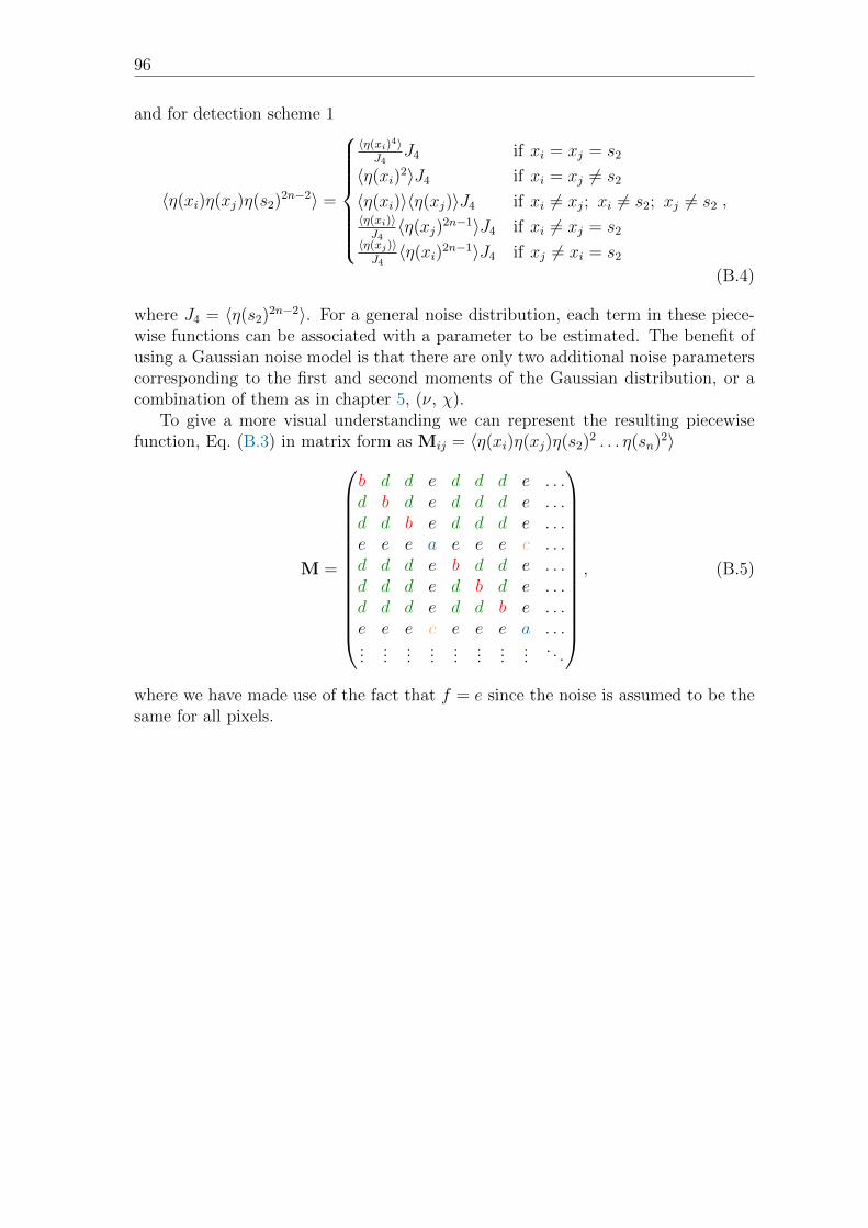
96
and for detection scheme 1
〈η(xi)η(xj)η(s2)2n−2〉 =
〈η(xi)4〉
J4J4 if xi = xj = s2
〈η(xi)2〉J4 if xi = xj 6= s2
〈η(xi)〉〈η(xj)〉J4 if xi 6= xj; xi 6= s2; xj 6= s2〈η(xi)〉J4〈η(xj)
2n−1〉J4 if xi 6= xj = s2〈η(xj)〉J4〈η(xi)
2n−1〉J4 if xj 6= xi = s2
,
(B.4)
where J4 = 〈η(s2)2n−2〉. For a general noise distribution, each term in these piece-wise functions can be associated with a parameter to be estimated. The benefit ofusing a Gaussian noise model is that there are only two additional noise parameterscorresponding to the first and second moments of the Gaussian distribution, or acombination of them as in chapter 5, (ν, χ).
To give a more visual understanding we can represent the resulting piecewisefunction, Eq. (B.3) in matrix form as Mij = 〈η(xi)η(xj)η(s2)2 . . . η(sn)2〉
M =
b d d e d d d e . . .d b d e d d d e . . .d d b e d d d e . . .e e e a e e e c . . .d d d e b d d e . . .d d d e d b d e . . .d d d e d d b e . . .e e e c e e e a . . ....
......
......
......
.... . .
, (B.5)
where we have made use of the fact that f = e since the noise is assumed to be thesame for all pixels.
Bibliography
[Aaronson and Arkhipov, 2010] Aaronson, S. and Arkhipov, A. (2010). The Com-putational Complexity of Linear Optics. page 94, 1011.3245.
[Aaronson and Arkhipov, 2013] Aaronson, S. and Arkhipov, A. (2013). BosonSam-pling Is Far From Uniform. page 41, 1309.7460.
[Abbe, 1873] Abbe, E. (1873). Beitrage zur Theorie des Mikroskops und dermikroskopischen Wahrnehmung. Arch. fur Mikroskopische Anat., 9(1):413–418.
[Agafonov et al., 2008a] Agafonov, I., Chekhova, M., Iskhakov, T., and Penin, A.(2008a). High-visibility multiphoton interference of Hanbury Brown–Twiss typefor classical light. Phys. Rev. A, 77(5):053801.
[Agafonov et al., 2008b] Agafonov, I. N., Chekhova, M. V., Iskhakov, T. S., andPenin, A. N. (2008b). High-visibility multiphoton interference of hanbury brown-twiss type for classical light. Phys. Rev. A, 77:053801.
[Agafonov et al., 2009a] Agafonov, I. N., Chekhova, M. V., Iskhakov, T. S., andWu, L.-A. (2009a). High-visibility intensity interference and ghost imaging withpseudo-thermal light. J. Mod. Opt., 56(2-3):422–431.
[Agafonov et al., 2009b] Agafonov, I. N., Chekhova, M. V., and Penin, A. N.(2009b). Multiphoton ghost imaging with classical light. 0911.3718.
[Barnett and Radmore, 1997] Barnett, S. M. and Radmore, P. M. (1997). Methodsin Theoretical Quantum Optics. Oxford University Press.
[Bennink et al., 2002] Bennink, R., Bentley, S., and Boyd, R. (2002). “Two-Photon”Coincidence Imaging with a Classical Source. Phys. Rev. Lett., 89(11).
[Beran and Parrent, 1964] Beran, M. J. and Parrent, G. B. (1964). Theory of PartialCoherence. Prentice-Hall.
[Blomstedt et al., 2013] Blomstedt, K., Setala, T., Tervo, J., Turunen, J., andFriberg, A. T. (2013). Partial polarization and electromagnetic spatial coherenceof blackbody radiation emanating from an aperture. Phys. Rev. A, 88(1):013824.
[Born and Wolf, 1980] Born, M. and Wolf, E. (1980). Principles of Optics. Cam-bridge University Press, 6th edition.
[Boto et al., 2000] Boto, A., Kok, P., Abrams, D., Braunstein, S., Williams, C., andDowling, J. (2000). Quantum Interferometric Optical Lithography: ExploitingEntanglement to Beat the Diffraction Limit. Phys. Rev. Lett., 85(13):2733–2736,9912052.
97
98 BIBLIOGRAPHY
[Brainis, 2010] Brainis, E. (2010). Huygens-Fresnel principle for N-photon states oflight. page 5, 1011.1402.
[Brannen and Ferguson, 1956] Brannen, E. and Ferguson, H. I. S. (1956). TheQuestion of Correlation between Photons in Coherent Light Rays. Nature,178(4531):481–482.
[Braunstein and Caves, 1994] Braunstein, S. and Caves, C. (1994). Statistical dis-tance and the geometry of quantum states. Phys. Rev. Lett., 72(22):3439–3443.
[Braunstein et al., 1996] Braunstein, S. L., Caves, C. M., and Milburn, G. (1996).Generalized Uncertainty Relations: Theory, Examples, and Lorentz Invariance.Ann. Phys. (N. Y)., 247(1):135–173.
[Brown and Twiss, 1956a] Brown, R. H. and Twiss, R. Q. (1956a). A test of a newtype of stellar interferometer on Sirius. Nature, 178:1046–1048.
[Brown and Twiss, 1956b] Brown, R. H. and Twiss, R. Q. (1956b). Correlationbetween Photons in two Coherent Beams of Light. Nature, 177(4497):27–29.
[Brown and Twiss, 1957] Brown, R. H. and Twiss, R. Q. (1957). Interferometry ofthe Intensity Fluctuations in Light. I. Basic Theory: The Correlation betweenPhotons in Coherent Beams of Radiation. Proc. R. Soc. A Math. Phys. Eng. Sci.,242(1230):300–324.
[Brown and Twiss, 1958a] Brown, R. H. and Twiss, R. Q. (1958a). Interferometryof the Intensity Fluctuations in Light II. An Experimental Test of the Theory forPartially Coherent Light. Proc. R. Soc. Lond. A. Math. Phys. Sci., 243(1234):291–319.
[Brown and Twiss, 1958b] Brown, R. H. and Twiss, R. Q. (1958b). Interferometryof the Intensity Fluctuations in Light. III. Applications to Astronomy. Proc. R.Soc. Lond. A. Math. Phys. Sci., 248(1253):199–221.
[Brown and Twiss, 1958c] Brown, R. H. and Twiss, R. Q. (1958c). Interferometryof the Intensity Fluctuations in Light. IV. A Test of an Intensity Interferometeron Sirius A. Proc. R. Soc. Lond. A. Math. Phys. Sci., 248(1253):222–237.
[Cahill and Glauber, 1969] Cahill, K. E. and Glauber, R. J. (1969). Density opera-tors and quasiprobability distributions. Phys. Rev., 177(5):1882–1902.
[Cao et al., 2008] Cao, D., Xiong, J., and Zhang, S. (2008). Enhancing visibilityand resolution in¡ equation¿ N¡ font face=’verdana’¿ th¡/font¿¡/equation¿-orderintensity correlation of thermal light. Appl. Phys. . . . .
[Chan et al., 2009] Chan, K. W. C., O’Sullivan, M. N., and Boyd, R. W. (2009).High-order thermal ghost imaging. Opt. Lett., 34(21):3343–5.
[Chen et al., 2010] Chen, X.-H., Agafonov, I. N., Luo, K.-H., Liu, Q., Xian, R.,Chekhova, M. V., and Wu, L.-A. (2010). High-visibility, high-order lensless ghostimaging with thermal light. Opt. Lett., 35(8):1166–8.
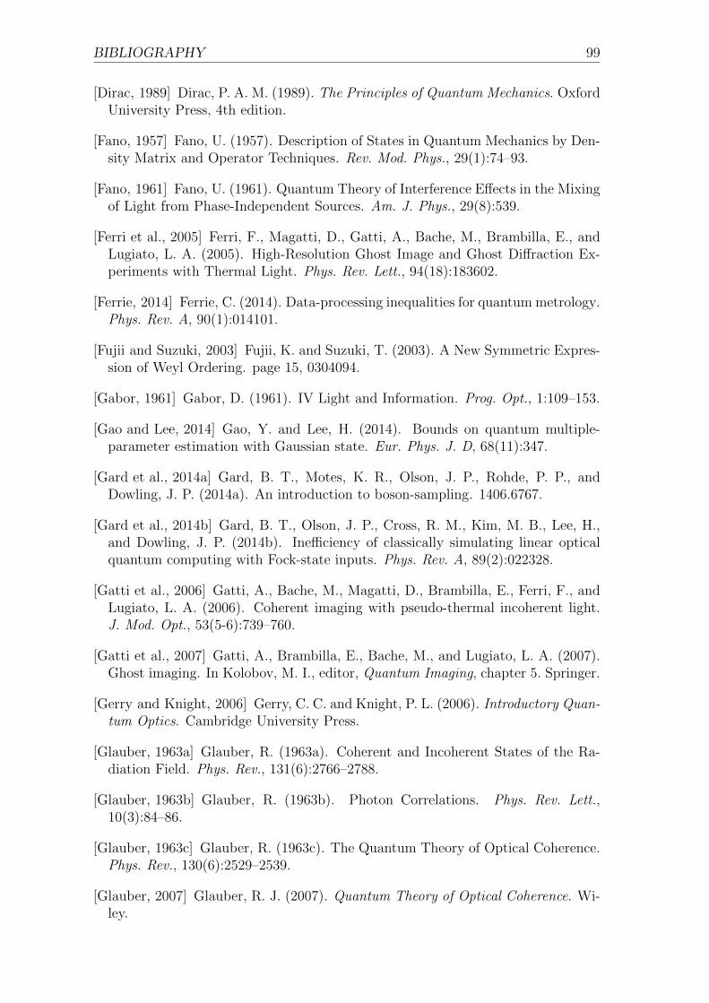
BIBLIOGRAPHY 99
[Dirac, 1989] Dirac, P. A. M. (1989). The Principles of Quantum Mechanics. OxfordUniversity Press, 4th edition.
[Fano, 1957] Fano, U. (1957). Description of States in Quantum Mechanics by Den-sity Matrix and Operator Techniques. Rev. Mod. Phys., 29(1):74–93.
[Fano, 1961] Fano, U. (1961). Quantum Theory of Interference Effects in the Mixingof Light from Phase-Independent Sources. Am. J. Phys., 29(8):539.
[Ferri et al., 2005] Ferri, F., Magatti, D., Gatti, A., Bache, M., Brambilla, E., andLugiato, L. A. (2005). High-Resolution Ghost Image and Ghost Diffraction Ex-periments with Thermal Light. Phys. Rev. Lett., 94(18):183602.
[Ferrie, 2014] Ferrie, C. (2014). Data-processing inequalities for quantum metrology.Phys. Rev. A, 90(1):014101.
[Fujii and Suzuki, 2003] Fujii, K. and Suzuki, T. (2003). A New Symmetric Expres-sion of Weyl Ordering. page 15, 0304094.
[Gabor, 1961] Gabor, D. (1961). IV Light and Information. Prog. Opt., 1:109–153.
[Gao and Lee, 2014] Gao, Y. and Lee, H. (2014). Bounds on quantum multiple-parameter estimation with Gaussian state. Eur. Phys. J. D, 68(11):347.
[Gard et al., 2014a] Gard, B. T., Motes, K. R., Olson, J. P., Rohde, P. P., andDowling, J. P. (2014a). An introduction to boson-sampling. 1406.6767.
[Gard et al., 2014b] Gard, B. T., Olson, J. P., Cross, R. M., Kim, M. B., Lee, H.,and Dowling, J. P. (2014b). Inefficiency of classically simulating linear opticalquantum computing with Fock-state inputs. Phys. Rev. A, 89(2):022328.
[Gatti et al., 2006] Gatti, A., Bache, M., Magatti, D., Brambilla, E., Ferri, F., andLugiato, L. A. (2006). Coherent imaging with pseudo-thermal incoherent light.J. Mod. Opt., 53(5-6):739–760.
[Gatti et al., 2007] Gatti, A., Brambilla, E., Bache, M., and Lugiato, L. A. (2007).Ghost imaging. In Kolobov, M. I., editor, Quantum Imaging, chapter 5. Springer.
[Gerry and Knight, 2006] Gerry, C. C. and Knight, P. L. (2006). Introductory Quan-tum Optics. Cambridge University Press.
[Glauber, 1963a] Glauber, R. (1963a). Coherent and Incoherent States of the Ra-diation Field. Phys. Rev., 131(6):2766–2788.
[Glauber, 1963b] Glauber, R. (1963b). Photon Correlations. Phys. Rev. Lett.,10(3):84–86.
[Glauber, 1963c] Glauber, R. (1963c). The Quantum Theory of Optical Coherence.Phys. Rev., 130(6):2529–2539.
[Glauber, 2007] Glauber, R. J. (2007). Quantum Theory of Optical Coherence. Wi-ley.
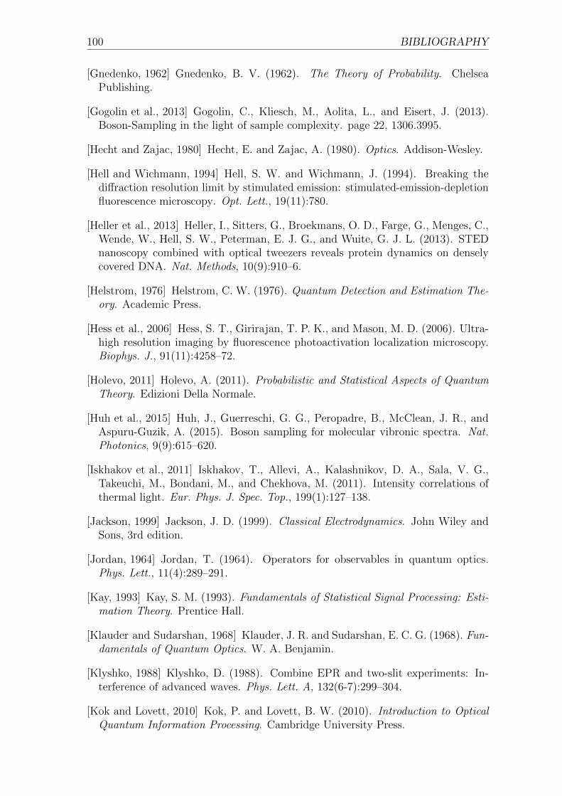
100 BIBLIOGRAPHY
[Gnedenko, 1962] Gnedenko, B. V. (1962). The Theory of Probability. ChelseaPublishing.
[Gogolin et al., 2013] Gogolin, C., Kliesch, M., Aolita, L., and Eisert, J. (2013).Boson-Sampling in the light of sample complexity. page 22, 1306.3995.
[Hecht and Zajac, 1980] Hecht, E. and Zajac, A. (1980). Optics. Addison-Wesley.
[Hell and Wichmann, 1994] Hell, S. W. and Wichmann, J. (1994). Breaking thediffraction resolution limit by stimulated emission: stimulated-emission-depletionfluorescence microscopy. Opt. Lett., 19(11):780.
[Heller et al., 2013] Heller, I., Sitters, G., Broekmans, O. D., Farge, G., Menges, C.,Wende, W., Hell, S. W., Peterman, E. J. G., and Wuite, G. J. L. (2013). STEDnanoscopy combined with optical tweezers reveals protein dynamics on denselycovered DNA. Nat. Methods, 10(9):910–6.
[Helstrom, 1976] Helstrom, C. W. (1976). Quantum Detection and Estimation The-ory. Academic Press.
[Hess et al., 2006] Hess, S. T., Girirajan, T. P. K., and Mason, M. D. (2006). Ultra-high resolution imaging by fluorescence photoactivation localization microscopy.Biophys. J., 91(11):4258–72.
[Holevo, 2011] Holevo, A. (2011). Probabilistic and Statistical Aspects of QuantumTheory. Edizioni Della Normale.
[Huh et al., 2015] Huh, J., Guerreschi, G. G., Peropadre, B., McClean, J. R., andAspuru-Guzik, A. (2015). Boson sampling for molecular vibronic spectra. Nat.Photonics, 9(9):615–620.
[Iskhakov et al., 2011] Iskhakov, T., Allevi, A., Kalashnikov, D. A., Sala, V. G.,Takeuchi, M., Bondani, M., and Chekhova, M. (2011). Intensity correlations ofthermal light. Eur. Phys. J. Spec. Top., 199(1):127–138.
[Jackson, 1999] Jackson, J. D. (1999). Classical Electrodynamics. John Wiley andSons, 3rd edition.
[Jordan, 1964] Jordan, T. (1964). Operators for observables in quantum optics.Phys. Lett., 11(4):289–291.
[Kay, 1993] Kay, S. M. (1993). Fundamentals of Statistical Signal Processing: Esti-mation Theory. Prentice Hall.
[Klauder and Sudarshan, 1968] Klauder, J. R. and Sudarshan, E. C. G. (1968). Fun-damentals of Quantum Optics. W. A. Benjamin.
[Klyshko, 1988] Klyshko, D. (1988). Combine EPR and two-slit experiments: In-terference of advanced waves. Phys. Lett. A, 132(6-7):299–304.
[Kok and Lovett, 2010] Kok, P. and Lovett, B. W. (2010). Introduction to OpticalQuantum Information Processing. Cambridge University Press.
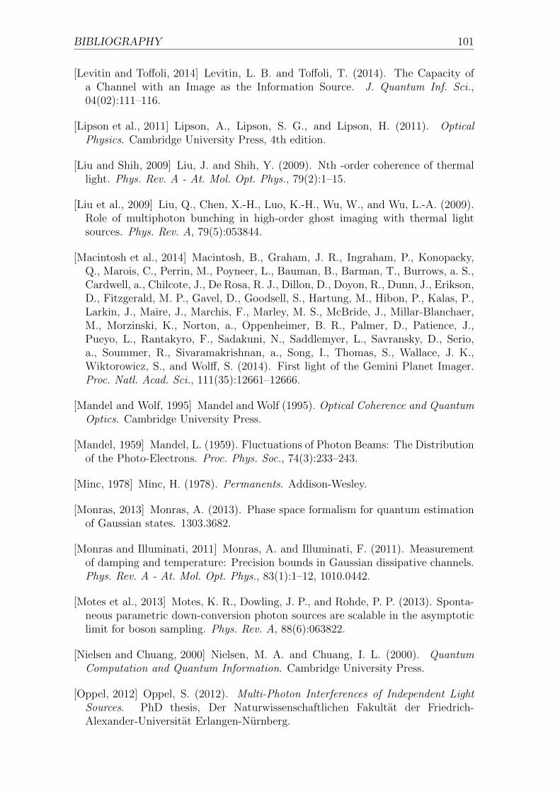
BIBLIOGRAPHY 101
[Levitin and Toffoli, 2014] Levitin, L. B. and Toffoli, T. (2014). The Capacity ofa Channel with an Image as the Information Source. J. Quantum Inf. Sci.,04(02):111–116.
[Lipson et al., 2011] Lipson, A., Lipson, S. G., and Lipson, H. (2011). OpticalPhysics. Cambridge University Press, 4th edition.
[Liu and Shih, 2009] Liu, J. and Shih, Y. (2009). Nth -order coherence of thermallight. Phys. Rev. A - At. Mol. Opt. Phys., 79(2):1–15.
[Liu et al., 2009] Liu, Q., Chen, X.-H., Luo, K.-H., Wu, W., and Wu, L.-A. (2009).Role of multiphoton bunching in high-order ghost imaging with thermal lightsources. Phys. Rev. A, 79(5):053844.
[Macintosh et al., 2014] Macintosh, B., Graham, J. R., Ingraham, P., Konopacky,Q., Marois, C., Perrin, M., Poyneer, L., Bauman, B., Barman, T., Burrows, a. S.,Cardwell, a., Chilcote, J., De Rosa, R. J., Dillon, D., Doyon, R., Dunn, J., Erikson,D., Fitzgerald, M. P., Gavel, D., Goodsell, S., Hartung, M., Hibon, P., Kalas, P.,Larkin, J., Maire, J., Marchis, F., Marley, M. S., McBride, J., Millar-Blanchaer,M., Morzinski, K., Norton, a., Oppenheimer, B. R., Palmer, D., Patience, J.,Pueyo, L., Rantakyro, F., Sadakuni, N., Saddlemyer, L., Savransky, D., Serio,a., Soummer, R., Sivaramakrishnan, a., Song, I., Thomas, S., Wallace, J. K.,Wiktorowicz, S., and Wolff, S. (2014). First light of the Gemini Planet Imager.Proc. Natl. Acad. Sci., 111(35):12661–12666.
[Mandel and Wolf, 1995] Mandel and Wolf (1995). Optical Coherence and QuantumOptics. Cambridge University Press.
[Mandel, 1959] Mandel, L. (1959). Fluctuations of Photon Beams: The Distributionof the Photo-Electrons. Proc. Phys. Soc., 74(3):233–243.
[Minc, 1978] Minc, H. (1978). Permanents. Addison-Wesley.
[Monras, 2013] Monras, A. (2013). Phase space formalism for quantum estimationof Gaussian states. 1303.3682.
[Monras and Illuminati, 2011] Monras, A. and Illuminati, F. (2011). Measurementof damping and temperature: Precision bounds in Gaussian dissipative channels.Phys. Rev. A - At. Mol. Opt. Phys., 83(1):1–12, 1010.0442.
[Motes et al., 2013] Motes, K. R., Dowling, J. P., and Rohde, P. P. (2013). Sponta-neous parametric down-conversion photon sources are scalable in the asymptoticlimit for boson sampling. Phys. Rev. A, 88(6):063822.
[Nielsen and Chuang, 2000] Nielsen, M. A. and Chuang, I. L. (2000). QuantumComputation and Quantum Information. Cambridge University Press.
[Oppel, 2012] Oppel, S. (2012). Multi-Photon Interferences of Independent LightSources. PhD thesis, Der Naturwissenschaftlichen Fakultat der Friedrich-Alexander-Universitat Erlangen-Nurnberg.

102 BIBLIOGRAPHY
[Oppel et al., 2012] Oppel, S., Buttner, T., Kok, P., and von Zanthier, J. (2012).Superresolving Multiphoton Interferences with Independent Light Sources. Phys.Rev. Lett., 109(23):233603.
[Paris, 2009] Paris, M. (2009). Quantum estimation for quantum technology. Int.J. Quantum Inf.
[Pearce et al., 2015] Pearce, M. E., Mehringer, T., von Zanthier, J., and Kok, P.(2015). Precision estimation of source dimensions from intensity correlation func-tions. In preparation.
[Pendry, 2000] Pendry, J. B. (2000). Negative Refraction Makes a Perfect Lens.Phys. Rev. Lett., 85(18):3966–3969.
[Perelomov, 1986] Perelomov, A. (1986). Generalized Coherent States and TheirApplications. Springer-Verlag.
[Perez-Delgado et al., 2012] Perez-Delgado, C., Pearce, M., and Kok, P. (2012).Fundamental Limits of Classical and Quantum Imaging. Phys. Rev. Lett., 109(12).
[Pittman et al., 1995] Pittman, T. B., Shih, Y. H., Strekalov, D. V., and Sergienko,A. V. (1995). Optical imaging by means of two-photon quantum entanglement.Phys. Rev. A, 52(5):R3429–R3432.
[Purcell, 1956] Purcell, E. M. (1956). Question of correlation between photons incoherent light rays. Nature, 178:1449–50.
[Rayleigh, 1879] Rayleigh, L. (1879). XXXI. Investigations in optics, with specialreference to the spectroscope. Philos. Mag. Ser. 5, 8(49):261–274.
[Reed, 1962] Reed, I. (1962). On a moment theorem for complex Gaussian processes.IRE Trans. Inf. Theory, 8(3):0–1.
[Rust et al., 2006] Rust, M. J., Bates, M., and Zhuang, X. (2006). Sub-diffraction-limit imaging by stochastic optical reconstruction microscopy (STORM). Nat.Methods, 3(10):793–5.
[Silva and Freire Jr, 2013] Silva, I. and Freire Jr, O. (2013). The Concept of the Pho-ton in Question: The Controversy Surrounding the HBT Effect circa 1956–1958.Hist. Stud. Nat. Sci., 43(4):453–491.
[Sudarshan, 1963] Sudarshan, E. (1963). Equivalence of Semiclassical and QuantumMechanical Descriptions of Statistical Light Beams. Phys. Rev. Lett., 10(7):277–279.
[Thiel et al., 2007] Thiel, C., Bastin, T., Martin, J., Solano, E., von Zanthier, J.,and Agarwal, G. (2007). Quantum imaging with incoherent photons. Phys. Rev.Lett, 99(13):133603.
[Titulaer and Glauber, 1965] Titulaer, U. M. and Glauber, R. J. (1965). CorrelationFunctions for Coherent Fields. Phys. Rev., 140(3B):B676–B682.
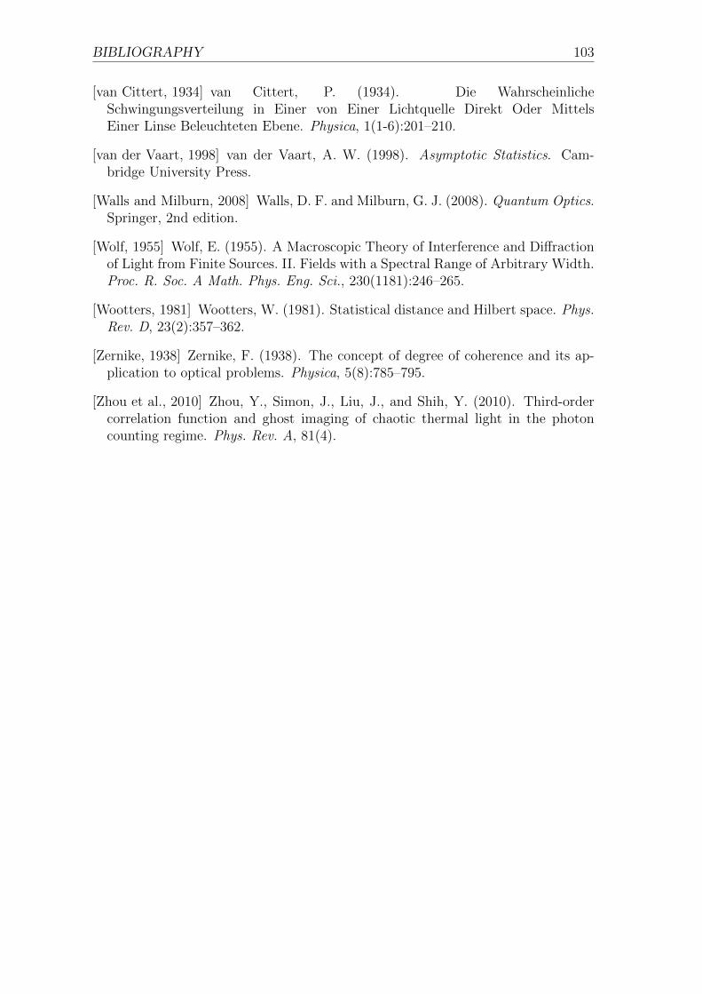
BIBLIOGRAPHY 103
[van Cittert, 1934] van Cittert, P. (1934). Die WahrscheinlicheSchwingungsverteilung in Einer von Einer Lichtquelle Direkt Oder MittelsEiner Linse Beleuchteten Ebene. Physica, 1(1-6):201–210.
[van der Vaart, 1998] van der Vaart, A. W. (1998). Asymptotic Statistics. Cam-bridge University Press.
[Walls and Milburn, 2008] Walls, D. F. and Milburn, G. J. (2008). Quantum Optics.Springer, 2nd edition.
[Wolf, 1955] Wolf, E. (1955). A Macroscopic Theory of Interference and Diffractionof Light from Finite Sources. II. Fields with a Spectral Range of Arbitrary Width.Proc. R. Soc. A Math. Phys. Eng. Sci., 230(1181):246–265.
[Wootters, 1981] Wootters, W. (1981). Statistical distance and Hilbert space. Phys.Rev. D, 23(2):357–362.
[Zernike, 1938] Zernike, F. (1938). The concept of degree of coherence and its ap-plication to optical problems. Physica, 5(8):785–795.
[Zhou et al., 2010] Zhou, Y., Simon, J., Liu, J., and Shih, Y. (2010). Third-ordercorrelation function and ghost imaging of chaotic thermal light in the photoncounting regime. Phys. Rev. A, 81(4).