Class Notes for Math 1110, Section 5 - Cornell Universitygoldberg/ClassNotes.pdfClass Notes for Math...

Class Notes for Math 1110, Section 5

Timothy Goldberg

Spring 2009

Contents

1 Day One: January 19 3

1.1 Introduction . . . . . . . . . . . . . . . . . . . . . . . . . . . . . . . . 3

1.2 Relations between quantities . . . . . . . . . . . . . . . . . . . . . . . 3

1.2.1 Equations . . . . . . . . . . . . . . . . . . . . . . . . . . . . . 3

1.2.2 Equations that are functions . . . . . . . . . . . . . . . . . . . 4

1.3 Functions in general . . . . . . . . . . . . . . . . . . . . . . . . . . . 5

1.4 Building new functions from old . . . . . . . . . . . . . . . . . . . . . 7

2 Day Two: January 21 10

2.1 Introduction . . . . . . . . . . . . . . . . . . . . . . . . . . . . . . . . 10

2.2 Properties of limits . . . . . . . . . . . . . . . . . . . . . . . . . . . . 11

2.3 Algebraic manipulations . . . . . . . . . . . . . . . . . . . . . . . . . 13

2.4 One-sided limits . . . . . . . . . . . . . . . . . . . . . . . . . . . . . . 15

3 Day Three: January 23 17

3.1 What do limits really mean? . . . . . . . . . . . . . . . . . . . . . . . 17

3.2 Limits at infinity . . . . . . . . . . . . . . . . . . . . . . . . . . . . . 19

4 Day Four: January 26 24

5 Day Five: January 28 25

6 Day Six: January 30 27

1

MATH 1110 Class Notes Section 5

7 Day Seven: February 2 28

8 Day Eight: February 4 29

9 Day Nine: February 6 31

10 Day Ten: February 9 32

11 Day Eleven: February 10 36

11.1 Increasing and decreasing . . . . . . . . . . . . . . . . . . . . . . . . 36

11.2 Approximating small changes . . . . . . . . . . . . . . . . . . . . . . 39

12 Day Twelve: February 13 42

12.1 Rates of change . . . . . . . . . . . . . . . . . . . . . . . . . . . . . . 42

12.2 Sensitivity to change . . . . . . . . . . . . . . . . . . . . . . . . . . . 43

12.3 Higher order derivatives . . . . . . . . . . . . . . . . . . . . . . . . . 44

13 Day Thirteen: February 16 49

14 Day Fourteen: February 18 49

14.1 Some announcements . . . . . . . . . . . . . . . . . . . . . . . . . . . 49

14.2 Some warm-up problems . . . . . . . . . . . . . . . . . . . . . . . . . 49

14.3 More higher order derivatives . . . . . . . . . . . . . . . . . . . . . . 50

14.4 Implicit functions . . . . . . . . . . . . . . . . . . . . . . . . . . . . . 52

15 Day Fifteen: February 20 55

15.1 Introduction . . . . . . . . . . . . . . . . . . . . . . . . . . . . . . . . 55

15.2 What is an implicit function? . . . . . . . . . . . . . . . . . . . . . . 55

15.3 Implicit differentiation . . . . . . . . . . . . . . . . . . . . . . . . . . 58

Remark. These are notes for Section 5 of Math 1110, taught at Cornell University

during the spring semester of 2009. This is a first-semester course in single variable

calculus. These notes are only meant to supplement reading from the textbook, not

replace it. They do not contain all the material necessary for this class.

2


1 Day One: January 19

1.1 Introduction

Calculus can be viewed as a collection of concepts and techniques that were in-

vented/discovered to answer the question, “How can we understand the nature of

changing quantities?” This differs from other mathematical topics, such as algebra

and geometry, which typically study static, unchanging situations.

Math 1110 is a first-semester calculus course. In broad strokes, it covers limits,

differentiation, integration, relations among them, and applications of each. I have

two objectives for this course. The first is to help you to learn, understand, and apply

the basic features of calculus, whose concepts and techniques are the foundation

for many other classes in mathematics and other fields. The second objective is

more general but equally important. It is to help you understand how mathematics

can be used to better grasp, analyze, and solve problems in all sorts of contexts.

Mathematics provides a way of thinking about situations and information in a logical

and systematic fashion. Helping you to develop this understanding and these skills

should be a part of every math course you take.

1.2 Relations between quantities

1.2.1 Equations

The most straightforward example of a relationship between quantities is an equation.

A = 2πr2, x2 + y2 = 1, y2 = x3 − x+ 1

The examples given here each expresses a relationship between only two quantities

— between A and r in the first case, and between x and y in the second and third.

But certainly there can be arbitrarily many quantities involved in an equation.

The big contribution of Descartes to mathematics was to realize that we can

literally picture equations (specifically, their solution sets), by assigning coordinates

to points in space. By putting an xy-axis on a plane, we can assign to each point a

unique coordinate (x, y). We form the graph of an equation involving the variables

x and y by coloring in each point in the plane whose coordinates (x, y) satisfy the

given equation.

3


-5 -2.5 0 2.5 5

-2.5

2.5

Figure 1: The circle is the graph of the equation x2 + y2 = 1. The other curve is the

graph of the equation y2 = x3 − x+ 1, called an elliptic curve.

Notice that it is a minor miracle that the graphs of most equations we encounter

form nice curves. If you randomly start coloring in points in the plane, there’s no

particular reason to think that they would form a curve.

1.2.2 Equations that are functions

The simplest kind of equation is one where one of the variables is alone on one side

of the equation.

y = x2 − 1

In this equation, the value of y is completely determined by the value of x. We say

that “y is a function of x”, and we can write y(x) = x2 − 1, or y = f(x) where

f(x) = x2 − 1. There are many different notations.

Because each value of x determines a specific value of y, the graph of an equation

involving x and y where y is a function of x will have a particularly nice prop-

erty. Above each value on the x-axis, there can be at most one point on the graph.

Otherwise, there would be two values of y that correspond to a single value of x.

Another way to characterize this property is called the vertical line test. An

equation gives y as a function of x if and only if it is impossible to draw a vertical

line in the plane going through more than one point on the graph. For instance,

notice that the circle pictured in Figure 1 fails the Vertical Line Test, so it cannot

be the graph of a function.

4


1.3 Functions in general

The concept of a function actually encompasses things much more general than just

those defined by equations.

Notation.

A set is a collection of objects. An element is an object in a set. The notation

“a ∈ A” means “a is an element of the set A”. The notation “B ⊂ A” means that

“the set B is a subset of the set A”, which simply means that every element of B

is also an element of A.

We denote the set of real numbers by the symbol R. The set of real numbers

includes all integers, fractions of integers, square roots, cube roots, et cetera. It

also includes transcendental numbers, like π and e. The real numbers exactly

consist of all possible decimal numbers, terminating and non-terminating, repeating

and non-repeating. The real numbers fill up the entire number line.

Non-examples of real numbers include, but are not limited to, the imaginary

unit i =√−1, all complex numbers such as 2 + 3i, and me, Timothy Goldberg.

Also, apples are not real numbers.

Example 1.1.

Consider the open interval (−1, 3), which consists of all real numbers x such that

−1 < x < 3. Then 0 ∈ (−1, 3), and (−1, 3) ⊂ R.

Definition 1.2.

A function f between two sets A and B is any assignment of an element f(a) ∈ Bto each element a ∈ A. We use the notation “f : A→ B” to denote such a function.

The set A of inputs is called the domain of f , and the set B of outputs is called the

codomain of f .

The set of elements of B which actually appear as outputs of f is called the

range, or image of f , denoted by f(A). (This notation is meant to remind you

that the range is what you get by dumping the entire domain into the function.) Of

course, f(A) ⊂ B.

For later reference, the symbol “:=” means “is defined to be equal to”, whereas

“=” just means “is equal to”.

It may be silly to have separate concepts for the codomain and the range. Why

don’t we only use the range, the set of things that can actually come out of the

5


function? The reason is that it is sometimes quite difficult to figure out what the

range of a given function is. It’s usually easier just to say what the output could be,

without having to peg down exactly what it is.

Example 1.3.

1. Most functions we will deal with in this course are real-valued functions,

which means they are of the form

f : R→ R.

In general, if we are given a function in the form of a formula, like f(x) = x2,

then we assume that it’s domain is the largest subset of R for which the formula

is defined. For instance, given the formula g(x) =√x− 2, we assume that the

domain of g is the set of x ∈ R such that x− 2 ≥ 0. Hence,

g : [2,∞)→ R.

2. Consider the function mother defined by

mother(x) := the mother of x.

For example, mother (Gwynneth Paltrow) = Blythe Danner. This is a func-

tion

mother : {people} → {people} .

Of course, we could have set the codomain to be the set {women}. The image

of this function is exactly the set of women who have given birth.

3. It’s important to realize that even though most function involving numbers

that we encounter are given as formulas, there are certainly others for which

there isn’t a formula. For example, consider the function favorite : R → Rdefined by

favorite(x) := the number of people enrolled in Section 5 of

Math 1110 this spring whose favorite number is x.

Of course, this function will be equal to 0 almost everywhere.

6


Remark 1.4.

A very important point to keep in mind is that when we write down a formula for

a function, like f(x) = cos(x2), the variable we use doesn’t matter. For this reason, it

is sometimes called a dummy variable. The following formulae all define the same

function.

cos(x2), cos(z2), cos(θ2), cos(42), cos

(,2)

1.4 Building new functions from old

Given two real-valued functions f, g : A→ R defined on some set A ⊂ R, because we

can add, subtract, multiply, and divide real numbers, we can construct several new

functions.

(f + g)(x) := f(x) + g(x)

(f − g)(x) := f(x)− g(x)

(f · g)(x) := f(x) · g(x)

(f/g)(x) :=f(x)

g(x)

The domains of f+g, f−g, and f ·g are all A, just like those of the original functions.

But since division by zero is undefined, the domain of f/g is the set

{x ∈ A such that g(x) 6= 0} .

This way of constructing new functions should be very familiar to you, so I won’t

include any example.

A more general way of creating new functions, one which does not depend on the

functions being real-valued, is function composition. Let A, B, and C be sets,

and let f : A→ B and g : B → C be functions. Their composition is the function

g ◦ f : A→ C defined by

(g ◦ f)(a) := g (f(a))

for all a ∈ A. Notice that if you want to form the composition g ◦f of two functions,

you have to be sure the output of the inner function f is allowed to be an input

of the outer function g.

Example 1.5.

7


Let f(x) = sin x and g(x) = x2 + 1. Then

(f ◦ g)(x) = f (g(x)) = f(x2 + 1

)= sin

(x2 + 1

)and

(g ◦ f)(x) = g (f(x)) = g (sinx) = (sin x)2 + 1 = sin2 x+ 1.

The last way of constructing new functions from old that we will describe is

piecewise-defined functions. In a piecewise-defined function, the domain is bro-

ken up into several pieces, and each piece is assigned a function. Consider the

following formula.

f(x) =

x2 if x < 0

3x if 0 ≤ x < 2

−2x+ 10 if x ≥ 2

This represents a function f : R→ R whose domain is split up into three pieces:

(−∞, 0), [0, 2), and [2,∞).

When you plug a particular value of x into f(x), the formula you use to evaluate it

depends on which piece of the domain contains that value of x. So

f(−1) = (−1)2 = 1,

f(1) = 3(1) = 3, and

f(3) = −2(3) + 10 = −6 + 10 = 4.

We will now give two important examples of piecewise-defined functions.

Example 1.6.

1. The absolute value function, |x|, can be defined by

|x| ={x if x ≥ 0

−x if x < 0.

A little thought, and perhaps working through a couple of examples, will show

that this definition agrees with the usual definition of the absolute value of a

number x as the distance between x and 0, or as the number x written without

its sign.

8


2. The signum function, sgn(x), can be defined by

sgn(x) =

{1 if x > 0

−1 if x < 0.

The signum function simply measures the sign of its input, and is undefined at

0. It is not hard to show that

sgn(x) =x

|x|=|x|x.

9


2 Day Two: January 21

2.1 Introduction

Today’s topic is Limits of Functions. To ease into this topic, consider the function

f(x) = x2−3x+2x−2

. We can factor the numerator and write

f(x) =x2 − 3x+ 2

x− 2=

(x− 2)(x− 1)

x− 2.

It is incredibly tempting to cancel the factor x− 2 from the numerator and denomi-

nator, leaving the function x−1. The question is, what is the difference between

the functions (x−2)(x−1)x−2

and x− 1?

For any value of x except x = 2, these two functions have the same value. For

x = 2, the first function is undefined but the second simply evaluates to 2 − 1 = 1.

So the only difference between the two functions is their domains. Therefore, the

graph of y = f(x) looks exactly like the graph of y = x− 1, except that it is missing

the point (2, 1). See Figure 2.

-5 -2.5 0 2.5 5

-2.5

2.5

Figure 2: The graph of f(x) = (x−2)(x−1)x−2

. It is exactly the line y = x− 1 with a hole

at the point (2, 1).

Even though the function f is not defined at 2, we can ask about its behavior

near 2. We can ask about the behavior of the values of f(x) as the number x

approaches 2. From our work above, we see that the value of f(x) will approach 1.

To record this fact, we use the notation

limx→2

f(x) = 1,

10


which is read as “the limit of f(x) as x goes to 2 is 1”.

In order to ask about the behavior of a function f(x) as x approaches a particular

number a ∈ R, it is evidently not necessary for f to be defined at a, but it is important

that f be defined for all numbers near a. Specifically, in order to ask about the limit

limx→a

f(x),

we require that there be an open interval I ⊂ R such that a ∈ R, and such that f

is defined on the set I − {a}.

Remark 2.1.

• The notation “{a}” means the set containing only the element a. The notation

“I − {a}” denotes the set consisting of every element of I except for a. Thus,

(−1, 2)− {0} = {x ∈ R such that − 1 < x < 2 and x 6= 0} .

• By an open interval, we mean any finite open interval such as (−1, 2), any

half-open interval such as (−∞, 1) or (0,∞), or the entire real line R =

(−∞,∞).

2.2 Properties of limits

Let a ∈ R.

1. For any constant c ∈ R, we have limx→a

c = c, because the value of a constant

function does not depend at all on the input.

2. Because it would be ridiculous to imagine otherwise, we have

limx→a

x = a.

(Notice that a is a particular number, while x is a dummy variable for both

the limit and the function of which we are taking the limit.)

11


3. Suppose f and g are functions, and that limx→a

f(x) = L and limx→a

g(x) = M , for

some numbers L,M ∈ R. Then

limx→a

[f(x) + g(x)] = L+M,

limx→a

[f(x)− g(x)] = L−M,

limx→a

[f(x) · g(x)] = L ·M, and

limx→a

f(x)

g(x)=

L

Mso long as M 6= 0.

So, the limit of a sum is the sum of the limits, the limit of a difference is the

difference of the limits, and so forth.

Definition 2.2.

A polynomial function (of a single variable) is any function that can be written

in the form

anxn + an−1x

n−1 + · · ·+ a1x+ a0

for some real numbers an, an−1, . . . , a1, a0 ∈ R. Examples include the functions

2, 3x+ 1, x3 − πx+ 2, and 300x335 − 83x45 + 2.

The class of polynomial functions includes all linear functions (ax + b) and all

constant functions.

A rational function (of a single variable) is any function that can be written in

the form f(x)g(x)

for polynomial functions f(x) and g(x). An example is the function

x− 3

x2 + 1.

Setting the denominator g(x) equal to 1, we see that the class of rational functions

includes all polynomial functions.

Using the properties of limits we have already stated, we now know how to

compute most limits of any rational function. For instance,

limx→5

x− 3

x2 + 1=

limx→5(x− 3)

limx→5(x2 + 1)

=(limx→5 x)− (limx→5 3)

(limx→5 x) · (limx→5 x) + (limx→5 1)

=5− 3

(5)(5) + 1=

2

26.

12


In the end, all we really did was plug the value x = 5 into the function. The only

thing that could have gone wrong is if the denominator had ended up being equal to

zero. This is exactly how one proves the following theorem.

Theorem 2.3. Let f be a rational function which is defined at the number a ∈ R.

Then

limx→a

f(x) = f(a).

2.3 Algebraic manipulations

What if we are trying to calculate the limit limx→a

f(x) of a rational function f(x) that

isn’t defined at x = a? Usually, the answer is to try some algebraic manipulation.

Example 2.4.

1. Question. Calculate the limit

limx→2

x2 − 3x+ 2

x− 2.

Answer. We saw above that x2−3x+2x−2

= (x−2)(x−1)x−2

, and hence x2−3x+2x−2

= x− 1

for all x ∈ R− {2}. Since the limit at 2 only cares what happens near 2, and

not at 2, we know that

limx→2

x2 − 3x+ 2

x− 2= lim

x→2

(x− 2)(x− 1)

x− 2= lim

x→2x− 1 = 2− 1 = 1.

In general, if we can perform an algebraic manipulation that only changes our

function at a finite number of points, then the limit will remain the same.

2. Question. Let a ∈ R be a fixed real number. Calculate the limit

limx→a

1x− 1

a

x− a.

Answer. This actually is a rational function, because it can be re-written in

the correct form. The trick is to combine the fractions in the numerator by

13


finding a common denominator. We calculate

limx→a

1x− 1

a

x− a= lim

x→a

aa· 1

x− x

x· 1

a

x− a

= limx→a

aax− x

ax

x− a

= limx→a

aax− x

ax

x− a

= limx→a

a−xax

x− a

= limx→a

−(x− a)

(x− a)(ax)

= limx→a− 1

ax= − 1

a2.

Note that our final answer doesn’t make sense if a = 0.


limx→4

√x− 2

x2 − 16.

Answer. There are certainly several different ways to do this, but the one

that comes first to my mind is to multiply the numerator by its conjugate.

Of course, to balance the fraction we must multiply the denominator by the

same thing. We calculate

limx→4

√x− 2

x2 − 16= lim

x→4

√x− 2

x2 − 16·√x+ 2√x+ 2

= limx→4

(√x− 2)(

√x+ 2)

(x2 − 16)(√x+ 2)

= limx→4

x− 4

(x− 4)(x+ 4)(√x+ 2)

= limx→4

1

(x+ 4)(√x+ 2)

=1

(4 + 4)(√

4 + 2)=

1

(8)(4)=

1

32.

14


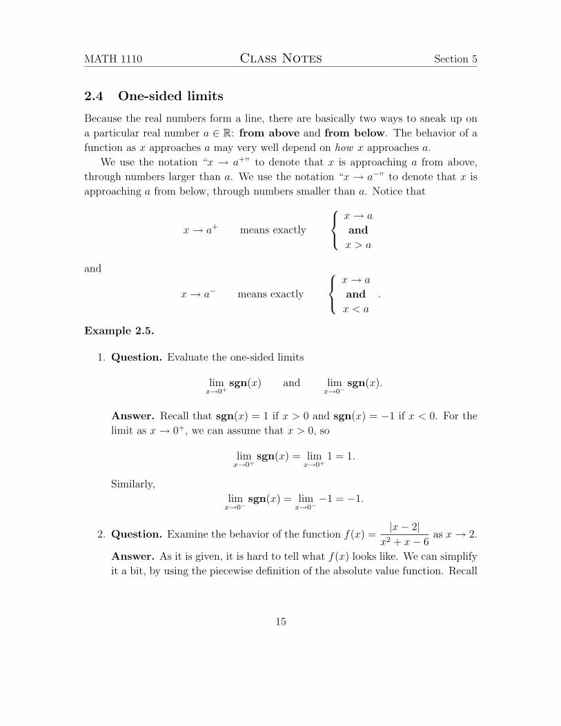
2.4 One-sided limits

Because the real numbers form a line, there are basically two ways to sneak up on

a particular real number a ∈ R: from above and from below. The behavior of a

function as x approaches a may very well depend on how x approaches a.

We use the notation “x → a+” to denote that x is approaching a from above,

through numbers larger than a. We use the notation “x → a−” to denote that x is

approaching a from below, through numbers smaller than a. Notice that

x→ a+ means exactly

x→ a

and

x > a

and

x→ a− means exactly

x→ a

and

x < a

.

Example 2.5.

1. Question. Evaluate the one-sided limits

limx→0+

sgn(x) and limx→0−

sgn(x).

Answer. Recall that sgn(x) = 1 if x > 0 and sgn(x) = −1 if x < 0. For the

limit as x→ 0+, we can assume that x > 0, so

limx→0+

sgn(x) = limx→0+

1 = 1.

Similarly,

limx→0−

sgn(x) = limx→0−

−1 = −1.

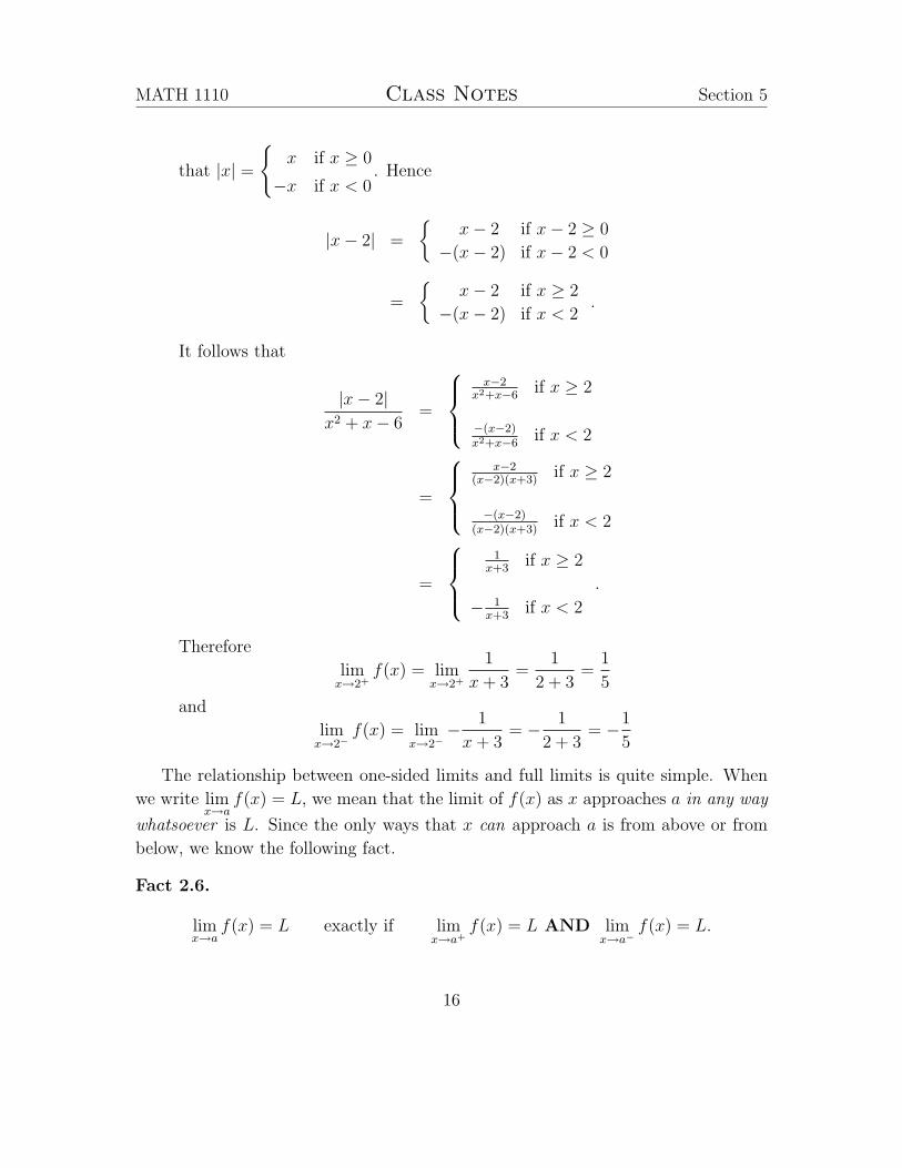
2. Question. Examine the behavior of the function f(x) =|x− 2|

x2 + x− 6as x→ 2.

Answer. As it is given, it is hard to tell what f(x) looks like. We can simplify

it a bit, by using the piecewise definition of the absolute value function. Recall

15


that |x| =

{x if x ≥ 0

−x if x < 0. Hence

|x− 2| =

{x− 2 if x− 2 ≥ 0

−(x− 2) if x− 2 < 0

=

{x− 2 if x ≥ 2

−(x− 2) if x < 2.

It follows that

|x− 2|x2 + x− 6

=

x−2

x2+x−6if x ≥ 2

−(x−2)x2+x−6

if x < 2

=

x−2

(x−2)(x+3)if x ≥ 2

−(x−2)(x−2)(x+3)

if x < 2

=

1

x+3if x ≥ 2

− 1x+3

if x < 2

.

Therefore

limx→2+

f(x) = limx→2+

1

x+ 3=

1

2 + 3=

1

5

and

limx→2−

f(x) = limx→2−

− 1

x+ 3= − 1

2 + 3= −1

5

The relationship between one-sided limits and full limits is quite simple. When

we write limx→a

f(x) = L, we mean that the limit of f(x) as x approaches a in any way

whatsoever is L. Since the only ways that x can approach a is from above or from

below, we know the following fact.

Fact 2.6.

limx→a

f(x) = L exactly if limx→a+

f(x) = L AND limx→a−

f(x) = L.

16


3 Day Three: January 23

3.1 What do limits really mean?

What exactly do we mean when we write

limx→a

f(x) = L?

Intuitively, we mean the following two things.

• As we take numbers x that are increasingly close to a, we obtain numbers f(x)

that are increasingly close to L.

• We can make f(x) as close to L as we want, so long as we make x really close

to a.

These conditions amount to the following working definition.

We write “limx→a

f(x) = L” if the value of

f(x) can be made arbitrarily close to L by

making x sufficiently close to a.

We measure the closeness of two numbers by calculating the distance between them,

and we do this by taking the absolute value of their difference. So f(x) and L are

close to each other exactly when |f(x) − L| is very small. So we can rewrite our

working definition as follows.

We write “limx→a

f(x) = L” if the distance

|f(x)−L| can be made arbitrarily small by

making the number |x−a| sufficiently small.

The terms “arbitrarily small” and “sufficiently small” are still not very precise. They

basically mean, if you tell me how small you want |f(x) − L| to be, I can tell you

how small you need to make |x−a| in order to make that happen. There’s a succinct

way to write this in mathematical language.

17


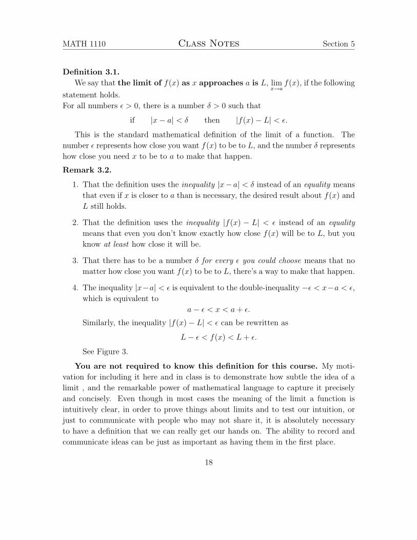
Definition 3.1.

We say that the limit of f(x) as x approaches a is L, limx→a

f(x), if the following

statement holds.

For all numbers ε > 0, there is a number δ > 0 such that

if |x− a| < δ then |f(x)− L| < ε.

This is the standard mathematical definition of the limit of a function. The

number ε represents how close you want f(x) to be to L, and the number δ represents

how close you need x to be to a to make that happen.

Remark 3.2.

1. That the definition uses the inequality |x− a| < δ instead of an equality means

that even if x is closer to a than is necessary, the desired result about f(x) and

L still holds.

2. That the definition uses the inequality |f(x) − L| < ε instead of an equality

means that even you don’t know exactly how close f(x) will be to L, but you

know at least how close it will be.

3. That there has to be a number δ for every ε you could choose means that no

matter how close you want f(x) to be to L, there’s a way to make that happen.

4. The inequality |x−a| < ε is equivalent to the double-inequality −ε < x−a < ε,

which is equivalent to

a− ε < x < a+ ε.

Similarly, the inequality |f(x)− L| < ε can be rewritten as

L− ε < f(x) < L+ ε.

See Figure 3.

You are not required to know this definition for this course. My moti-

vation for including it here and in class is to demonstrate how subtle the idea of a

limit , and the remarkable power of mathematical language to capture it precisely

and concisely. Even though in most cases the meaning of the limit a function is

intuitively clear, in order to prove things about limits and to test our intuition, or

just to communicate with people who may not share it, it is absolutely necessary

to have a definition that we can really get our hands on. The ability to record and

communicate ideas can be just as important as having them in the first place.

18


Figure 3: The graph of a function f(x) satisfying the condition: “if |x− a| < δ then

|f(x)− L| < ε”.

3.2 Limits at infinity

Just as we can ask about the behavior of a function f(x) as x gets infinitely close to

a number a, we can ask about its behavior as x gets infinitely large.

Definition 3.3.

We say the limit of f(x) as x approaches infinity is L, written

limx→∞

f(x) = L,

if f(x) can be made arbitrarily close to L by taking x sufficiently large.

Similarly, we say the limit of f(x) as x approaches negative infinity is L,

written

limx→−∞

f(x) = L,

if f(x) can be made arbitrarily close to L by taking x sufficiently large in the negative

direction.

Example 3.4.

Consider the function f(x) = 1x. When you divide 1 by a huge number you get a

small result, and the huger the number is the smaller the result. Hence limx→∞

1

x= 0.

19


The same thing holds if you divide 1 by a hugely negative number, so limx→−∞

1

x= 0

also. These facts are evident from the graph of 1x, shown in Figure 4.

The laws of limits we listed previously hold for limits at infinity as well. Hence,

for 1x2 = 1

x· 1

x, for 1

x3 = 1x· 1

x· 1

x, and in general for 1

xp for any positive integer p, we

have

limx→±∞

1

xp= 0.

This will prove to be an extremely valuable fact.

-5 -2.5 0 2.5 5

-2.5

2.5

Figure 4: The graph of 1x, which demonstrates that limx→±∞

1x

= 0. If we want to be

more precise about how the function approaches 0, we could write limx→∞1x

= 0+

and limx→−∞1x

= 0−, although usually this isn’t necessary.

Definition 3.5. The horizontal line y = L is a horizontal asymptote of f(x) if

limx→∞ f(x) = L or limx→−∞ f(x) = L, or both.

Since there are only two infinite limits to check, a function can have at most two

horizontal asymptotes. It could instead have no horizontal asymptotes, or it could

have only one. If a function has just a single horizontal line as an asymptote, it

could be an asymptote in the∞ direction only, in the −∞ direction only, or in both

directions at once. An example of this last situation is the function 1x, which has

y = 0 as a horizontal asymptote in both directions.

The graph of a function can cross its horizontal asymptote any number of times,

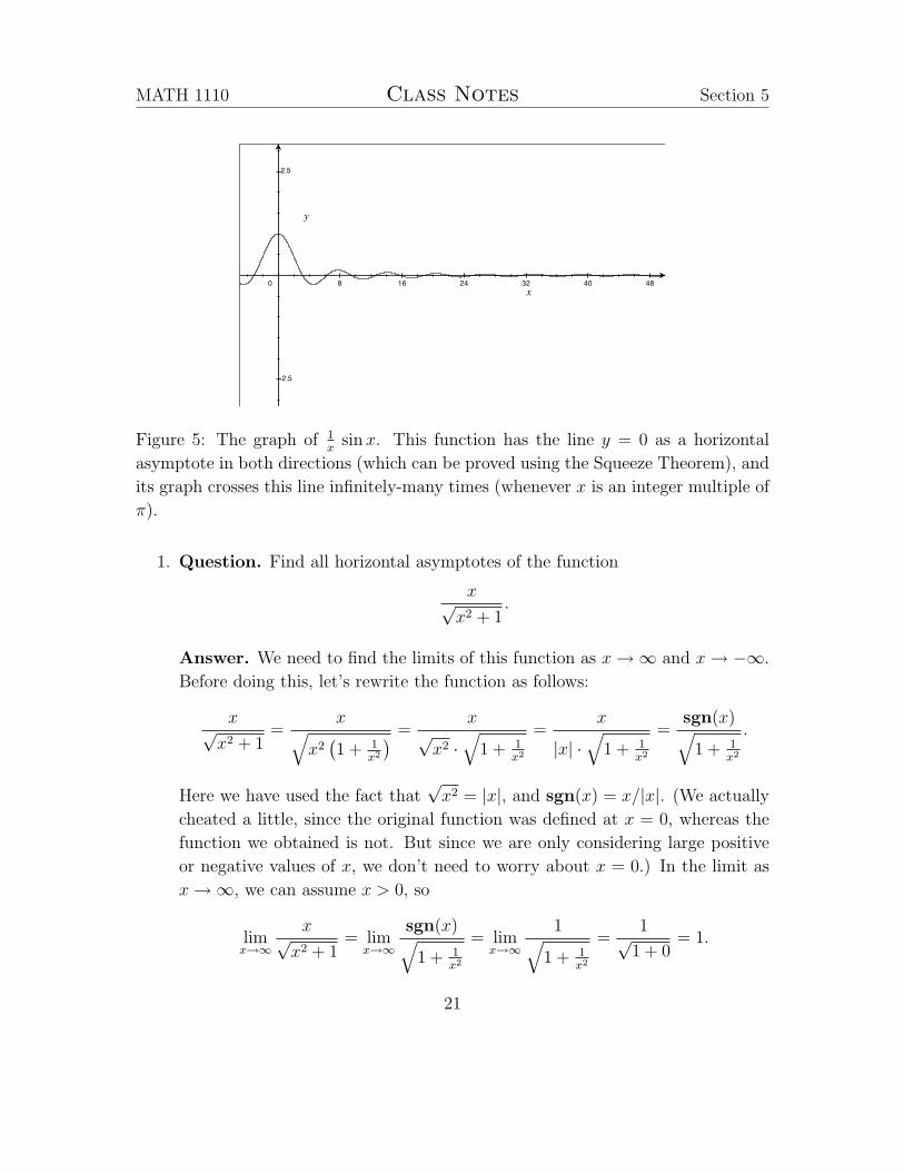
including infinitely-many. For example, see Figure 5.

Example 3.6.

20


0 8 16 24 32 40 48

-2.5

2.5

Figure 5: The graph of 1x

sinx. This function has the line y = 0 as a horizontal

asymptote in both directions (which can be proved using the Squeeze Theorem), and

its graph crosses this line infinitely-many times (whenever x is an integer multiple of

π).

1. Question. Find all horizontal asymptotes of the function

x√x2 + 1

.

Answer. We need to find the limits of this function as x→∞ and x→ −∞.

Before doing this, let’s rewrite the function as follows:

x√x2 + 1

=x√

x2(1 + 1

x2

) =x

√x2 ·

√1 + 1

x2

=x

|x| ·√

1 + 1x2

=sgn(x)√

1 + 1x2

.

Here we have used the fact that√x2 = |x|, and sgn(x) = x/|x|. (We actually

cheated a little, since the original function was defined at x = 0, whereas the

function we obtained is not. But since we are only considering large positive

or negative values of x, we don’t need to worry about x = 0.) In the limit as

x→∞, we can assume x > 0, so

limx→∞

x√x2 + 1

= limx→∞

sgn(x)√1 + 1

x2

= limx→∞

1√1 + 1

x2

=1√

1 + 0= 1.

21


Here we used the fact that 1x2 → 0 as x → ∞, and also the previously-

unmentioned fact that we can take limits under square root signs. Similarly,

limx→−∞

x√x2 + 1

= limx→−∞

sgn(x)√1 + 1

x2

= limx→−∞

− 1√1 + 1

x2

= − 1√1 + 0

= −1.

Therefore, this function has y = 1 as a horizontal asymptote in the positive

direction, and y = −1 as a horizontal asymptote in the negative direction.


2x2 − x+ 3

3x2 + 5.

Answer. The only functions whose behaviors at ±∞ we know are those of

the form 1xp for some positive integer p. There is a nice trick for transforming

any rational function into a combination of terms of this form, and that is to

divide both numerator and denominator by the highest power of x appearing in

the denominator. In the given function, that power term is x2, and we obtain

2x2 − x+ 3

3x2 + 5=

1x2 · (2x2 − x+ 3)

1x2 · (3x2 + 5)

=2− 1

x+ 3

x2

3 + 5x2

.

Therefore

limx→±∞

2x2 − x+ 3

3x2 + 5= lim

x→±∞

2− 1x

+ 3x2

3 + 5x2

=2− 0 + 0

3 + 0=

2

3.

Therefore y = 23

is a horizontal asymptote for this function in both directions.


5x+ 2

2x3 − 1.

Answer. In the given function, that power term is x3, and we obtain

limx→±∞

5x+ 2

2x3 − 1= lim

x→±∞

1x3 · (5x+ 2)1x3 · (2x3 − 1)

= limx→±∞

5x2 + 2

x3

2− 1x3

=0 + 0

2− 0=

0

2= 0.

Therefore y = 0 is a horizontal asymptote for this function in both directions.

22



limx→∞

(√x2 + x− x

).

Answer. A little thought reveals that both√x2 + x and x go to∞ as x→∞,

and so it is incredibly tempting to conclude that this limit equals∞−∞, which

must surely be 0. But this is wrong. The infinity symbol ∞represents a behavior, NOT a number. To calculate

this limit, we need to use a little algebra to change the form of the function.

We have

limx→∞

(√x2 + x− x

)= lim

x→∞

(√x2 + x− x

)·

(√x2 + x+ x√x2 + x+ x

)

= limx→∞

(√x2 + x− x)(

√x2 + x+ x)√

x2 + x+ x

= limx→∞

(x2 + x)− x2

√x2 + x+ x

= limx→∞

x√x2 + x+ x

= limx→∞

x√x2(1 + 1

x

)+ x

= limx→∞

x√x2 ·

√1 + 1

x+ x

= limx→∞

1x· (x)

1x·(|x| ·

√1 + 1

x+ x)

= limx→∞

1

sgn(x) ·√

1 + 1x

+ 1

=1

1 ·√

1 + 0 + 1=

1

2.

23


4 Day Four: January 26

We discussed what it means for a function to be continuous, and why continuous

functions are so nice. The main definition is that a function f(x) is continuous at

a point x = a if

limx→a

= f(a).

We noted that almost all the functions we know, except piecewise functions, are

continuous.

One of the main reasons continuous functions are nice is that we can calculate

their limits as x → a by simply plugging in x = a. Two other nice properties of

continuous functions are the Extreme Value Theorem (also known as the Min-

Max Theorem), and the Intermediate Value Theorem.

Theorem 4.1 (Extreme Value Theorem). Let [a, b] be a closed and finite interval,

and let f be a continuous function on [a, b]. Then there are numbers m and M

in the interval [a, b] such that f(m) is a minimum of f on [a, b] and f(M) is a

maximum of f on [a, b]; i.e.

f(m) ≤ f(x) ≤ f(M)

for all x in [a, b].

Theorem 4.1 says not only that a continuous function on a closed and finite

interval is bounded, but that it achieves its bounds.

Theorem 4.2 (Intermediate Value Theorem). Let [a, b] be a closed and finite in-

terval, and let f be a continuous function on [a, b]. If s is any number between

f(a) and f(b), then there exists a point c in the interval [a, b] such that

f(c) = s.

Theorems 4.1 and 4.2 are together equivalent to the following fact.

Theorem 4.3. A continuous function maps closed, finite intervals to closed, finite

intervals. In other words, if f is continuous on the closed, finite interval [a, b], then

there are numbers c < d such that the image of f is

f([a, b]

)= [c, d].

24


5 Day Five: January 28

The most common way to define a tangent line to a graph is as a limit of secant

lines to the graph. Suppose we want to identify the tangent line to the graph of

a function f(x) at the point on the graph with x-coordinate x0. To define a line,

we need a point on the line and the line’s slope. The line will contain the point(x0, f(x0)

). To determine its slope, consider the secant line of f over the closed

interval [x0, x], which is the line through the points(x0, f(x0)

)and

(x, f(x)

). As

x → x0, these points will move closer and closer to each other, and the secant line

over the interval [x0, x] will become more and more like the tangent line at x0. The

slope of this secant line is

msec,[x0,x] :=f(x)− f(x0)

x− x0

,

which is sometimes called a difference quotient. We define the slope of the tangent

line at x0 to be

mtan,x0 := limx→x0

msec,[x0,x] = limx→x0

f(x)− f(x0)

x− x0

.

Therefore an equation for this tangent line is

y − f(x0) = mtan,x0

(x− x0

).

Another common way of writing the definition of the slope of the tangent line is

to let h = x − x0. Then x = x0 + h and saying that x → x0 is the same as saying

that h→ 0. Hence the difference quotient may be written as

msec,[x0,x0+h] =f(x0 + h)− f(x0)

h,

and the tangent slope may be defined by

mtan,x0 := limh→0

msec,[x0,x0+h] = limh→0

f(x0 + h)− f(x0)

h.

To summarize, the tangent line is the limit of secant lines, and the slope of the

tangent line is the limit of the slopes of the secant lines.

25


To figure out what’s going on, sometimes we have to consider the two one-sided

limits of the difference quotient:

limh→0+

f(x0 + h)− f(x0)

hand lim

h→0+

f(x0 + h)− f(x0)

h.

If these are both equal to ∞ or −∞, then the tangent line is a vertical line. If

these two one-sided limits are different finite numbers, then the graph of f(x) has

a corner at x = x0. If these two one-sided limits are different infinities, then the

graph of f(x) has a cusp at x = x0, which is an extreme version of a corner.

26


6 Day Six: January 30

The derivative of a function f is a new function f ′ defined by

f ′(x) := limh→0

f(x+ h)− f(x)

h= mtan,x.

Of course, this limit may not be defined at all points, so the domain of f ′ may be

a strictly smaller set than the domain of f . The process of calculating f ′ is called

differentiation. If f ′(x) is defined at x = x0, we say f is differentiable at x0. If

f ′(x) is not defined at x = x0, we say f is singular at x0.

We noted that the derivative of a constant function is zero, the derivative of a

linear function is its slope, and the derivative of |x| is sgn(x). We also stated the

Power Rule:d

dxxr = r xr−1,

which holds for any real number r and for any value of x for which the expressions

on both sides make sense. We definitely did not prove the Power Rule, although a

fairly easy proof in the case that r is a positive integer can be found on page 101 of

the textbook.

27


7 Day Seven: February 2

We covered some basic properties of the derivative, including Linearity, the Prod-

uct Rule, and the Quotient Rule. These tell us that if f and g are differentiable

at x, and if c is any real number, then

d

dx

[c · f(x)

]= c · f ′(x),

=d

dx

[f(x) + g(x)

]= f ′(x) + g′(x),

=d

dx

[f(x) · g(x)

]= f ′(x) · g(x) + f(x) · g′(x), and

=d

dx

[f(x)

g(x)

]=

f ′(x) · g(x)− f(x) · g′(x)[g(x)

]2 .

This last equality only holds, of course, when g(x) 6= 0.

We also proved that differentiability implies continuity. The other direction

of this statement is not true, as evidenced by the function |x|, which is continuous

at x = 0 but not differentiable there.

28


8 Day Eight: February 4

We discussed the Chain Rule,

d

dxf(g(x)

)= f ′

(g(x)

)· g′(x),

which holds for any x such that g is differentiable at x and f is differentiable at

g(x). The Chain Rule implies that the composition of differentiable functions is

differentiable.

Morally speaking, the Chain Rule holds because when we compose two linear

functions, we get another linear function whose slope is the product of the slopes of

the original two lines.

For a function f and a point x = a, the linearization of f at a is the function

whose graph is the tangent line to the graph of f at x = a. Since this tangent line

has equation

y − f(a) = f ′(a) ·(x− a

),

the linearization of f at a is the function

Lf,a(x) := f ′(a) ·(x− a

)+ f(a).

Using the Chain Rule, we can prove the following (possibly) interesting result, which

you certainly will not be required to know for this class.

Theorem 8.1. Suppose the function g is differentiable at x = a and the function f

is differentiable at x = g(a). Then

Lf◦g,a = Lf,g(a) ◦ Lg,a.

Therefore, the tangent line to f ◦ g is the composition of a tangent line to f with a

tangent line to g.

Proof. The linearization of g at x = a is

Lg,a(x) = g′(a) ·(x− a

)+ g(a),

and the linearization of f at x = g(a) is

Lf,g(a)(x) = f ′(g(a)

)·(x− g(a)

)+ f(g(a)

).

29


Their composition is

Lf,g(a)

(Lg,a(x)

)= f ′

(g(a)

)·(Lg,a(x)− g(a)

)+ f(g(a)

)= f ′

(g(a)

)· Lg,a(x)− f ′

(g(a)

)· g(a) + f

(g(a)

)= f ′

(g(a)

)·(g′(a) ·

(x− a

)+ g(a)

)− f ′

(g(a)

)· g(a) + f

(g(a)

)= f ′

(g(a)

)· g′(a) ·

(x− a

)+ f ′

(g(a)

)· g(a)− f ′

(g(a)

)· g(a) + f

(g(a)

)= f ′

(g(a)

)· g′(a) ·

(x− a

)+ f(g(a)

).

By the Chain Rule, we have f ′(g(a)

)· g′(a) = (f ◦ g)′(a), and of course f

(g(a)

)=

(f ◦ g)(a). Therefore this last equation above is equal to

(f ◦ g)′(a) ·(x− a

)+ (f ◦ g)(a),

which is exactly Lf◦g,a.

30


9 Day Nine: February 6

We went through a brief review of trigonometry, and discussed the derivatives of the

trigonometric functions sine, cosine, tangent, secant, cosecant, and cotangent.

We also discussed the important limits

limx→0

sinx

x= 1 and lim

x→0

cosx− 1

x= 0,

which are secretly the derivatives

d

dxsinx

∣∣∣∣x=0

= limh→0

sinh

hand

d

dxcosx

∣∣∣∣x=0

= limh→0

cosh− 1

h.

31


10 Day Ten: February 9

Rolle’s Theorem states that if the graph of a differentiable function over a closed

interval comes back to the same y-value at which it started, then it must have had

a horizontal tangent line at some point.

Theorem 10.1 (Rolle’s Theorem). Let [a, b] be a closed and finite interval, and let f

be a function that is continuous on [a, b] and differentiable on (a, b). If f(a) = f(b),

then there is a number c in the interval (a, b) such that

f ′(c) = 0.

Figure 6: A graphical depiction of Rolle’s Theorem.

Example 10.2. Suppose you are tossing a ball up into the air and catch it, and

suppose that you toss it and throw it from the same height off the floor. Let y(t)

denote the ball’s height off the floor t seconds after you throw it, and suppose it

spends exactly 3 seconds in the air. Assuming the the height of the ball is a con-

tinuous and differentiable function of time, which is probably true as far as we can

really measure these things, Rolle’s Theorem tells us that there is a time t0 between

0 and 3 seconds such that y′(t0) = 0.

Of course, this is nothing too exciting. The derivative y′(t) measures the ball’s

upwards velocity at time t, and we know from experience that when the ball is at its

peak height, it’s velocity is zero.

Geometrically, Rolle’s Theorem is saying that if the secant line of the graph of f

over the closed interval [a, b] is horizontal, then the graph has a horizontal tangent

32


line. The Mean Value Theorem says that this fact does not depend on the secant

line being horizontal.

Theorem 10.3 (Mean Value Theorem). Let [a, b] be a closed and finite interval,

and let f be a function that is continuous on [a, b] and differentiable on (a, b). Then

there is some point c in the interval (a, b) such that

f ′(c) =f(b)− f(a)

b− a.

In other words, there is a tangent line to the graph of f that is parallel to the

secant line of the graph over the interval [a, b].

Figure 7: A graphical depiction of the Mean Value Theorem.

Remark 10.4.

1. Notice that Rolle’s Theorem is exactly the Mean Value Theorem in the case

that the secant slope is zero, which happens precisely when f(b) − f(a) = 0,

i.e. when f(a) = f(b).

33


2. Like the Extreme Value Theorem and the Intermediate Value Theorem, Rolle’s

Theorem and the Mean Value Theorem are both examples of existence the-

orems. They assure us that a point with a certain property exists, but they

give us no clue as to how to find it.

3. Both Rolle’s Theorem and the Mean Value Theorem tell us that there is at least

one tangent line to the function’s graph that is parallel to the secant line over

the whole interval, but there could be any number of such tangent lines. For

instance, in Figure 7 there are two points on the graph of f(x) whose tangent

lines are parallel to the red secant line.

Example 10.5.

Suppose Tim wants to drive from his apartment in Ithaca to the Carousel Cen-

ter Mall in Syracuse. Let x(t) be the distance in miles Tim has traveled from his

apartment t hours after he started on his adventure. According to Google maps, the

trip is about 55.6 miles and should take about 1.25 hours, and let us assume that it

is and that it does. Then

x(0) = 0 and x(1.25) = 55.6.

Recall that Tim’s average speed on this trip is the quotient of the total distance

and the total time taken, which is 55.6/1.25 = 44.48 miles per hour. Of course, this

is also the slope of the secant line of the graph of x(t) over the t-interval [0, 1.25]:

x(1.25)− x(0)

1.25− 0= 44.48.

Assuming Tim’s distance traveled is a continuous and differentiable function of time,

the Mean Value Theorem tells us that there is some time t = t0 such that x′(t0) =

44.48. Just as the slope of the secant line over a time interval represents the average

speed over that period of time, the slope of the tangent line at a particular time

represents the instantaneous speed at that time. We conclude that there must

have been a time during Tim’s trip when he was driving exactly 44.48 miles per hour.

This demonstrates a general principal, that most of us probably all know without

being aware of it. During any trip, there is always a point when the speed at which we

are driving is exactly the same as our average speed over the entire trip. Naturally,

sometimes we may drive faster than the average, and sometimes slower, but at some

point we have to hit it right on the nose.

34


Example 10.6.

Question. Prove that if x > 0 then x > sinx.

Answer. A priori, there is no reason to think that the Mean Value Theorem will

help us with this. The very clever trick is to realize that if x > 0, then saying that

sinx < x is exactly the same as saying that sin xx< 1, and that

sinx

x=

sinx− 0

x− 0=

sinx− sin 0

x− 0

is the slope of the secant line for the sine graph over the closed interval [0, x].

Let’s do the easy case first. If x > 1, then since sinx ≤ 1 we know that x > sinx.

Now suppose that x ≤ 1. Since the sine function is differentiable everywhere, we

can apply the Mean Value Theorem to it over the closed interval [0, x]. We conclude

that there is some number c in the open interval (0, x) such that the tangent slope

to the sine curve at c is equal to the secant slope over the interval [0, x], which we

saw above is sin xx

. The tangent slope in question is

d

dxsinx

∣∣∣∣x=c

= cosx|x=c = cos c,

so sin xx

= cos c. Now, recall that cos θ is strictly less than 1 if 0 < θ < 2π. Since

0 < cx ≤ 1 < π, we know cos c < 1. Therefore

sinx

x< 1,

so

sinx < x.

This completes the solution.

35


0 0.8 1.6 2.4 3.2 4 4.8 5.6

2.5

5

Figure 8: If x > 0, then x > sinx.

11 Day Eleven: February 10

11.1 Increasing and decreasing

Definition 11.1. Let f be a function defined on an interval I.

• f is increasing on I if for all x, y ∈ I,

x < y =⇒ f(x) < f(y).

• f is decreasing on I if for all x, y ∈ I,

x < y =⇒ f(x) > f(y).

• f is nondecreasing on I if for all x, y ∈ I,

x < y =⇒ f(x) ≤ f(y).

• f is nonincreasing on I if for all x, y ∈ I,

x < y =⇒ f(x) ≥ f(y).

• f is stationary on I if for all x, y ∈ I we have f(x) = f(y).

(The symbol =⇒ means “implies that”. For example, “x < y =⇒ f(x) < f(y)”

means “if x < y then f(x) < f(y)”.)

36


Remark 11.2.

1. If y = f(x), then to say that f is increasing means that if we make x bigger,

then y gets bigger. The meaning of decreasing can be explained similarly.

2. The difference between increasing and nondecreasing is the following. Sup-

pose y = f(x) and we make x bigger. If f is increasing, then y will definitely

get bigger, but if f is only nondecreasing, then y will either get bigger or

stay the same. The difference between decreasing and nonincreasing can

be explained similarly.

3. Saying that f is stationary is the same as saying that f is constant.

Theorem 11.3. Let f be a function defined on an interval I. Let J be the set

of interior points of I, (i.e. J consists of all points of I that aren’t endpoints).

Suppose f is continuous on I and differentiable on J .

• If f ′ > 0 on J then f is increasing on I.

• If f ′ < 0 on J then f is decreasing on I.

• If f ′ ≥ 0 on J then f is nondecreasing on I.

• If f ′ ≤ 0 on J then f is nonincreasing on I.

• If f ′ = 0 on J then f is stationary on I.

Remark 11.4.

1. It is fair to say that this theorem seems obvious, because we know that positive

derivative means that tangent lines have positive slope, which means that the

graph of the function is going up as x increases, and similarly (but opposite) for

negative derivative. However, just because this theorem seems obvious for every

function and curve we can imagine does not mean it is true for every function

and curve that there is. Some of the most amazing topics in mathematics arose

from people trying to prove something “obvious” that turned out not to be true.

An example of this is the development of non-Euclidean geometries, which

can be pretty awesome.

37


2. The proof of this theorem relies on the Mean Value Theorem, and it is suggested

by Question 1 of Quiz 2. Basically, we are trying to determine whether f(x) <

f(y) or f(x) > f(y) when x < y, which is the same as determining whether

f(y)− f(x) > 0 or f(y)− f(x) < 0 when x < y. Since we know that y−x > 0,

if we can figure out the sign of the fraction

f(y)− f(x)

y − x

then we know the sign of f(y) − f(x). The Mean Value Theorem, applied to

the closed interval [x, y], tells us that this fraction is equal to f ′(c) for some c

in the interval (x, y). Therefore, if we know the sign of the derivative, then we

can figure out whether f(x) < f(y) or vice versa.

3. We already knew that the derivative of a constant function is zero. This the-

orem tells us the converse, that if a function has zero derivative then it is

constant.

Example 11.5.

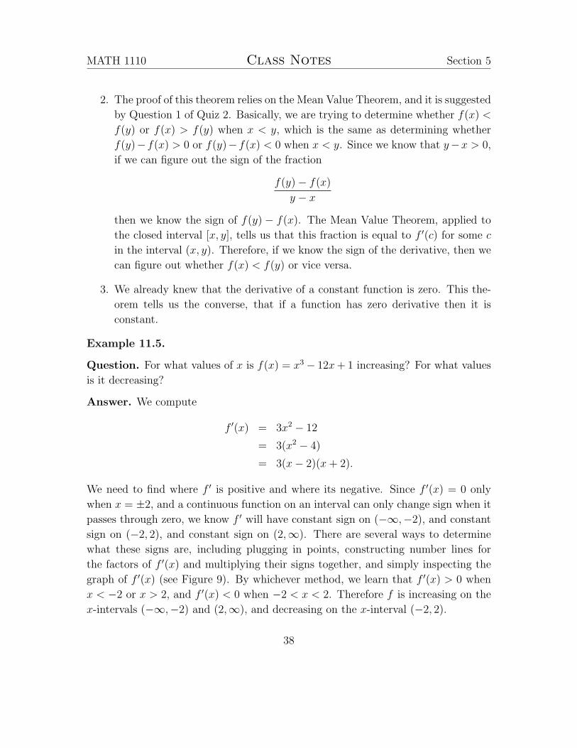
Question. For what values of x is f(x) = x3− 12x+ 1 increasing? For what values

is it decreasing?

Answer. We compute

f ′(x) = 3x2 − 12

= 3(x2 − 4)

= 3(x− 2)(x+ 2).

We need to find where f ′ is positive and where its negative. Since f ′(x) = 0 only

when x = ±2, and a continuous function on an interval can only change sign when it

passes through zero, we know f ′ will have constant sign on (−∞,−2), and constant

sign on (−2, 2), and constant sign on (2,∞). There are several ways to determine

what these signs are, including plugging in points, constructing number lines for

the factors of f ′(x) and multiplying their signs together, and simply inspecting the

graph of f ′(x) (see Figure 9). By whichever method, we learn that f ′(x) > 0 when

x < −2 or x > 2, and f ′(x) < 0 when −2 < x < 2. Therefore f is increasing on the

x-intervals (−∞,−2) and (2,∞), and decreasing on the x-interval (−2, 2).

38


-4 -3 -2 -1 0 1 2 3 4

-20

-10

10

20

Figure 9: The graph of f ′(x) = 3x2 − 12, from which one can deduce that f ′(x) > 0

when x < −2 or x > 2 and f ′(x) < 0 when −2 < x < 2.

11.2 Approximating small changes

Suppose y = f(x), and we know the value y0 = f(x0) of f at x0. If we add ∆x to x0,

how much does the value of the function f change from y0? In other words, what is

∆y := f(x0 + ∆x)− f(x0)?

In this section, we will learn how to estimate the function value f(x0 + ∆x) by

estimating ∆y.

Suppose the graph of f is a line of slope m. For a line, we know that the ratio ∆y∆x

of any change in y corresponding to a specified change in x is constant, and equals

the slope. Therefore, if f represents a line of slope m, then ∆y∆x

= m, so ∆y = m ·∆x,

so

f(x0 + ∆x) = f(x0) +m ·∆x.

Now let us go back to f being an arbitrary function. Note that

∆y

∆x=

f(x0 + ∆x)− f(x0)

(x0 + ∆x)− x0

= the slope of the secant line over the interval [x0, x0 + ∆x].

Now, if ∆x is small, then this secant slope is a good approximation of the tangent

slope at x0. Therefore ∆y∆x≈ f ′(x0), so

∆y ≈ f ′(x0) ·∆x

39


and

f(x0 + ∆x) ≈ f(x0) + f ′(x0) ·∆x.

Notice that whereas we usually use the secant slope to approximate the tangent

slope, in this case we are doing things the other way around.

To summarize, suppose we know the value f(x0) of a function f at a point x0, and

we want to know the value of f at the point x0 + ∆x. If ∆x is small and f ′(x0)

exists, then

∆y ≈ f ′(x0) ·∆x,

where ∆y is the difference between f(x0 + ∆x) and f(x0). Therefore

f(x0 + ∆x) ≈ f(x0) + f ′(x0) ·∆x.

Example 11.6.

Question. Suppose you draw a circle of radius r0 cm. By approximately how many

cm2 will the area of this circle increase if you increase the radius by 2 cm?

Answer. The radius r of a circle and its area A are related by the equation A = πr2.

The relationship between ∆A and ∆r is

∆A ≈ dA

dr·∆r = 2πr∆r.

In this example, we are starting with r = r0 and ∆r = 2, so

∆A ≈ 2πr∆r = 2πr0 · 2 = 4πr0.

Therefore the area will increase by approximately 4πr0 cm2.

The importance of a change ∆x depends on the context, i.e. on how big x is. If

you are measuring the length of a room, a mistake of 10 ft. is pretty important, but

this same mistake is far less important if you are measuring the length of a highway.

Therefore we make the following definition.

Definition 11.7. Let x be a quantity, and let ∆x be a specific change in that

quantity. The relative change in x is ∆xx

, and the percentage change in x is

100 · ∆xx

.

40


In relative change, we are taking our starting value of x as one unit, and the rel-

ative change represents the number of these units by which the quantity is changing.

Therefore, a relative change of 1 means that our quantity has doubled.

The percentage change is simply the relative change represented as a percentage.

Therefore, a percentage change of 100% means that our quantity has doubled.

Example 11.8.

Question. Suppose you increase the radius of a circle by 3%. By what percentage

have you increased the area of the circle?

Answer. As in the previous example, we have A = πr2 and ∆A ≈ dAdr·∆r = 2πr∆r.

The relative change in A is

∆A

A=

2πr∆r

πr2= 2 · ∆r

r.

Since the relative change in r is ∆rr

= 3% = 3100

, we conclude that the relative change

in A is∆A

A= 2 · ∆r

r= 2 · 3

100=

6

100,

so the area of the circle increased by 6%.

41


12 Day Twelve: February 13

12.1 Rates of change

By now, you may already be familiar with the following definitions.

Definition 12.1. Let f(x) be a function.

• The average rate of change of the function f with respect to x over the

x-interval [a, a+ h] is the slope of the secant line over this interval:

f(a+ h)− f(a)

h.

• The instantaneous rate of change of the function f with respect to x at

the x-value a is the slope of the tangent line at this point (if it exists):

f ′(a) = limh→0

f(a+ h)− f(a)

h.

Example 12.2.

Question. How fast is the area of a circle increasing with respect to its radius when

the radius is 5 m?

Answer. The rate of change of the area with respect to the radius is

dA

dr= 2πr.

When r = 5 m, this rate of change is 2π · 5 = 10πm2/m. (Note that the units we use

for this rate of change are units of area per units of radius.

Related to the interpretation of derivatives as measuring instantaneous rates of

change, we have the following terminology. If f ′(x0) = 0, we say that the function

f is stationary at x0, and we call the point x0 a critical point of the function

f . Sometimes the corresponding point(x0, f(x0)

)on the graph of f is also called a

critical point.

Graphically, a critical point of f represents a location where the graph of f has

a horizontal tangent line.

42


12.2 Sensitivity to change

Verbatim from the textbook, “when a small change in x produces a large change in

the value of a function f(x), we say that the function is very sensitive to changes

in x”. Recall the approximation formula

∆y ≈ f ′(x0) ·∆x.

Here ∆y is the change in function value from x0 to x0 + ∆x, i.e. ∆y = f(x0 +

∆x)−f(x0). From this approximation, we see that generally speaking, the larger the

derivative f ′(x0), the more sensitive the function f(x) to changes in x near x = x0.

Therefore, the derivative f ′(x) measures the sensitivity to change of f(x) with

respect to x.

Example 12.3 (Example 4, page 134 from the textbook). Suppose a pharmacol-

ogist studying a drug that has been developed to lower blood pressure determines

experimentally that the average reduction R in blood pressure from a daily dosage

of xmg of the drug is

R = 24.2

(1 +

x− 13√x2 − 26x+ 529

)mmHg.

(The units used here for measuring blood pressure are millimeters of mercury.) The

daily dose of many medications is 5 mg, 15 mg, or 35 mg. A natural question to ask

is this. For patients on which of these daily doses of the medication will a small

increase in dosage have the greatest effect?

What we are really asking about is the sensitivity in R to changes in x, which

is measured by the derivative dRdx

. Through arduous computation (as shown in the

textbook), one can compute that

dR

dx

∣∣∣∣x=5

≈ 0.998,dR

dx

∣∣∣∣x=15

≈ 1.254, anddR

dx

∣∣∣∣x=35

≈ 0.355.

The greatest sensitivity of R to change in x occurs when x = 15 mg, at which point

an increase in dosage by just 1 mg will yield an average reduction in blood pressure

of approximately (1 mg

)(1.254 mmHg/mg

)= 1.254 mmHg.

43


There are many applications of derivatives to economics. Some of these are

described in the textbook on pages 134–135. Generally speaking, this material is not

terribly important in this course, so I will not spend any time on it here. But, your

homework includes a couple of questions about this material, so you should probably

give it a read. If you will be required to know it for any exam in this course, I will

be sure to let you know.

12.3 Higher order derivatives

The derivative of a function f is a new function, which we denote by f ′. What we

have done once, we can do again, and define f ′′ to be the derivative of the f ′. We

call f ′′ the second derivative of f . If y = f(x), there are many different ways to

denote the second derivative, including

y′′ = f ′′(x) =d2y

dx2=

d2

dx2f(x) = D2

x f(x).

The notation d2ydx2 comes from

y′′ :=

(d

dx

)(d

dx

)y =

(d

dx

)2

y =d2y

dx2,

and the fact that we treat dx as a single symbol, so that its square is dx2.

Of course, we can go further, and consider the third derivative of f , denoted f ′′′,

the fourth derivative of f , denoted f ′′′′, and so forth. In general, for any positive

integer n we can consider the nth derivative of f . If y = f(x), the nth derivative

is denoted

y(n) = f (n)(x) =dny

dxn=

dn

dxnf(x) = Dn

x f(x).

For convenience, we define the 0th derivative of f just to be itself, f (0) := f . This

is what you get when you differentiate f zero times!

Remark 12.4.

1. Just as the derivative of f may not be defined at every point in the domain of

f , the second derivative f ′′ may not be defined at every point in the domain

of f ′. Thus

· · ·Dom(f ′′′) ⊂ Dom(f ′′) ⊂ Dom(f ′) ⊂ Dom(f).

If f (n)(x0) exists, we say that f in n times differentiable at x0.

44


2. Recall that if f is differentiable at x0, then f must be continuous at x0. For

the same reason, if f is twice differentiable at x0, then we know that f ′ is

continuous at x0, and in particular that f ′(x0) exists.

Example 12.5.

1. Consider the function

f(x) =

{x2 if x ≥ 0

−x2 if x < 0,

whose graph is given in Figure 10. It is not too hard to show that f ′(x) = |x|,and hence f ′′(x) = sgn(x). Therefore f(x) is differentiable at x = 0, but not

twice differentiable there.

-2 -1.6 -1.2 -0.8 -0.4 0 0.4 0.8 1.2 1.6 2

-2.5

2.5

Figure 10: The graph of f(x) from Example 12.5 (a). This function is differentiable

at x = 0, but not twice differentiable there.

2. Suppose f(x) = x3 + 3x2 + 5. Then

f ′(x) = 3x2 + 6x,

f ′′(x) = 6x+ 6,

f ′′′(x) = 6,

f (4)(x) = 0, and

f (5)(x) = 0.

Since the derivative of 0 is 0, we see that f (n)(x) = 0 for all integers n > 3.

45


3. Suppose f(x) = sinx. Then

f ′(x) = cosx,

f ′′(x) = − sinx,

f ′′′(x) = − cosx,

f (4)(x) = sinx,

f (5)(x) = cosx,

and the pattern continues. Therefore we can calculate that

d1001

dx1001sinx =

d

dxsinx = cosx,

because 1001 = 4× 250 + 1 and every four derivative of the sine function come

back to the sine function.

Besides being mathematically interesting, higher order derivatives are indescrib-

ably useful in applications. Perhaps the most common instance of this is in physics,

which is the subject that calculus was essentially invented to study in the first place.

Suppose an object moves in a straight line. For convenience, let’s slap an x-axis

onto this line of motion, and at time t denote the position of the object on this axis

by x(t). The velocity of the object at time t is

v(t) := x′(t) =d

dtx(t),

and the acceleration of the object at time t is

a(t) := v′(t) =d

dtv(t) =

d2

dt2x(t).

Thus, the velocity is the rate of change of position with respect to time, and the

acceleration is the rate of change of velocity with respect to time, which is the rate

of change of the rate of change of position with respect to time. If this x-axis is in its

standard position, with large positive values to the right and large negative values

to the left, then the signs of x(t), v(t), and a(t) can be interpreted as shown in the

following table.

46


x(t) > 0 object is to the right of the origin

x(t) < 0 object is to the left of the origin

x(t) = 0 object is at the origin (at this instant)

v(t) > 0 object is moving to the right

v(t) < 0 object is moving to the left

v(t) = 0 object is not moving (at this instant)

a(t) > 0 object’s motion to the right is speeding up

object’s motion to the left is slowing down

a(t) < 0 object’s motion to the left is speeding up

object’s motion to the right is slowing down

a(t) = 0 object is moving at constant speed (at this instant)

47


At the beginning of this course, we spoke of how relationships between quantities

can sometimes be expressed as equations. We can sometimes express relationships

between quantities and their rates of change as differential equations. A differ-

ential equation is an equation involving an unknown function and its derivatives,

such as

y′ = y.

(In fact, this differential equation is extremely important, and we will discuss it at

length in the near future.) Again, notice that whereas for usual equations we are

trying to solve for an unknown number, in differential equations we are trying to

solve for an unknown function.

Solving differential equations can be incredibly difficult — indeed, a significant

portion of the most interesting topics in mathematics have their roots in the study

of differential equations. In this course, with very few exceptions you will not be

required to solve any differential equations. What you will be expected to be able to

do is verify that a given function is a solution to a particular differential equation.

Example 12.6.

Question. Verify that for any constants A, B, and k, the function y = A cos(kt) +

B sin(kt) is a solution to the differential equation

d2y

dx2+ k2y = 0.

Answer. Using the Chain Rule, we compute

dy

dx= −kA sin(kt) + kB cos(kt)

andd2y

dx2= −k2A cos(kt)− k2B sin(kt).

Therefore

d2y

dx2+ k2y = −k2A cos(kt)− k2B sin(kt) + k2 (A cos(kt) +B sin(kt))

= −k2A cos(kt) + k2A cos(kt)− k2B sin(kt) + k2B sin(kt)

= 0

as desired.

48


13 Day Thirteen: February 16

We reviewed for Prelim One.

14 Day Fourteen: February 18

14.1 Some announcements

Today: office hours 3:30 PM – 4:30 PM

Tomorrow: office hours 11:30 AM – 12:30 PM

Sometime soon: Answers to Prelim One will be posted on Moodle.

Monday, February 23: Graded Prelims will be returned to you.

Monday, March 2: Prelim corrections are due.

Sometime after March 3: Full solutions to Prelim One will be posted on Moodle.

14.2 Some warm-up problems

Example 14.1.

Question. Suppose that a square is changing size. At the instant that its area is

100 m2, . . .

1. . . . what is the rate of change of the square’s area with respect to the length of

its sides?

2. . . . what is the rate of change of the square’s area with respect to the length of

its diagonals?

Answer. Let A be the area of the square, let x be the length of the square’s sides,

and let d be the length of the square’s diagonals. We know that A = x2, so dAdx

= 2x.

When 100 = A = x2 we have x =√

100 = 10 (where we use the positive square root

since x is measuring the length of something), so

dA

dx

∣∣∣∣x=10

= 2x|x=10 = 2 · 10 = 20 m2/m.

49


Notice that if we cut the square diagonally, we obtain an isosceles right triangle

with hypotenuse length d and leg length x. By the Pythagorean Theorem we have

d2 = x2 + x2 = 2x2. Therefore A = x2 = 12d2. Therefore dA

dd= 1

2· 2d = d. When

100 = A = 12d2 we have d =

√200 = 10

√2, so

dA

dd

∣∣∣∣d=10

√2

= 10√

2 m2/m.

Example 14.2.

Question. Prove that for any real number k, y = tan kx is a solution to the

differential equationd2y

dx2= 2k2y(1 + y2).

(HINT: Remember that sec2 θ = 1 + tan2 θ.)

Answer. We have dydx

= k sec2 kx, so

d2y

dx2=

d

dxk sec2 kx

= 2k sec kx ·(d

dxsec kx

)= 2k sec kx · sec kx · tan kx ·

(d

dxkx

)= 2k2 sec2 kx tan kx.

Using the trigonometric identity mentioned above, note that this is the same as

2k2y(1 + y2) = 2k2 tan kx(1 + tan2 kx

)= 2k2 tan kx sec2 kx,

so the differential equation is satisfied.

14.3 More higher order derivatives

Sometimes we can figure out a general formula, sometimes called a closed formula,

for the nth derivative of a particular function. This can be very useful when we start

talking about using Taylor polynomials to approximate functions.

50


Many of these formulas make use of the factorial function, which for any pos-

itive integer n is denoted n! and defined by

n! := n(n− 1) · (n− 2) · · · · · 3 · 2 · 1.

Despite the comedic value of doing so, the symbol “n!” is not read by shouting “n”

loudly.

By definition, we put 0! := 1. This may seem strange, except that n! is the

number of ways of ordering n objects, and there is really only one way to order no

objects. There, we just did it. And oops, we did it again!

Example 14.3.

1. If f(x) = xn, then f ′(x) = nxn−1 and f ′′(x) = n(n− 1)xn−2, and in general

f (k)(x) = n(n− 1)(n− 2) · · ·((n− (k − 1)

)xn−k

=

{n!

(n−k)!xn−k if 0 ≤ k ≤ n

0 if k > n.

2. Suppose y = 11+x

= (1 + x)−1. Then

y′ = −(1 + x)−2

y′′ = −(−2)(1 + x)−3 = 2(1 + x)−3

y′′′ = −3(2)(1 + x)−4 = −3!(1 + x)−4 and

y(4) = −4(−3!)(1 + x)−5 = 4!(1 + x)−5.

It seems pretty clear that

y(n) = (−1)n n!(1 + x)−(n+1) =(−1)n n!

(1 + x)n+1,

although it takes a little work to prove mathematically that this really is the

right formula.

Note our use of (−1)n to give us 1 if n is even and −1 if n is odd. This is a

handy little trick.

51


3. Suppose f(x) = sin(ax + b), where a and b are some constant real numbers.

Then

f ′(x) = a cos(ax+ b),

f ′′(x) = −a2 sin(ax+ b) = −a2 f(x),

f ′′′(x) = −a3 cos(ax+ b) = −a3 f ′(x),

f (4)(x) = a4 sin(ax+ b) = a4 f(x), and

f (4)(x) = a5 cos(ax+ b) = a5 f ′(x).

The derivatives alternate between f(x) = sin(ax + b) and f ′(x) = cos(ax + b)

at each step, change sign every other step, and at the nth step have a factor of

an out front. Therefore, it is safe to assume that

f (n)(x) =

{(−1)kan sin(ax+ b) if n = 2k for some k = 0, 1, 2, . . .

(−1)kan cos(ax+ b) if n = 2k + 1 for some k = 0, 1, 2, . . ..

Saying that n = 2k for some k = 0, 1, 2, . . . is another way of saying that n is

a nonnegative even integer, since every even integer can be written this way.

Similarly, n = 2k + 1 means that n is a nonnegative odd integer. Notice that

the use of (−1)k assures us that the sign will only change atevery other step,

whereas using (−1)n would make the sign change at every step.

14.4 Implicit functions

If a curve in the plane is actually the graph of a function, we know how to compute

the slopes of its tangent lines, which in turn can give us lots of useful information

about the curve. The goal of implicit differentiation is to be able to calculate the

slopes of tangent lines to curves that aren’t necessarily the graphs of functions, but

are given by some equation in x and y.

A simple example of such a thing is the equation

y2 = x,

whose corresponding curve in the xy-plane is a parabola opening to the right. We

know that this curve is not the graph of any function y = f(x), because it fails the

Vertical Line Test (infinitely-many times, in fact). But, one thing we can do is

52


-5 -4 -3 -2 -1 0 1 2 3 4 5

-2

-1

1

2

Figure 11: The curve corresponding to the equation y2 = x. Notice that it is not the

graph of any function y = f(x).

solve for y, obtaining the two equations

y1 =√x and y2 = −

√x.

These are functions, whose derivatives we can readily calculate:

y′1 =1

2√x

and y′2 = − 1

2√x.

Notice what is happening here.

Let C be the curve given by the equation

y2 = x.

• The part of C with y ≥ 0 is the graph

of the function y =√x.

• The part of C with y ≤ 0 is the graph

of the function y = −√x.

Definition 14.4. Given an equation in x and y, is there a way to restrict the values

of x and y so that the equation defines y as a function of x? In other words, by

making restrictions on the values of x and y, can we solve the equation for y?

If the answer is “yes”, then we say that the equation defines y implicitly as a

function of x.

53


This is a more general situation then where an equation in x and y is already

solved for y, in which case we say that the equation defines y explicitly as a

function of x. An example is the equation

y = x2 + sinx,

which clearly represents a function of x.

54


15 Day Fifteen: February 20

Remark 15.1. The examples in this day’s notes are actually a bit different from

those we did in class. In particular, there are a few more examples here than I

managed to present live in class.

15.1 Introduction

Today we will expand our differentiation techniques to enable us to determine the

slopes of tangent lines to a curve corresponding to an arbitrary equation involving

x and y. Often, a piece of such a curve is actually the graph of a function, in which

case this function is called an implicit function defined by the equation. If we can

figure out what these implicit functions are, then we can simply differentiate them to

obtain the tangent slopes. Unfortunately, this is often essentially impossible. Using

implicit differentiation, we will be able to find a formula for the slope dydx

of the

tangent line without having to find any implicit functions. The price we pay is that

this formula almost always involves both x and y.

15.2 What is an implicit function?

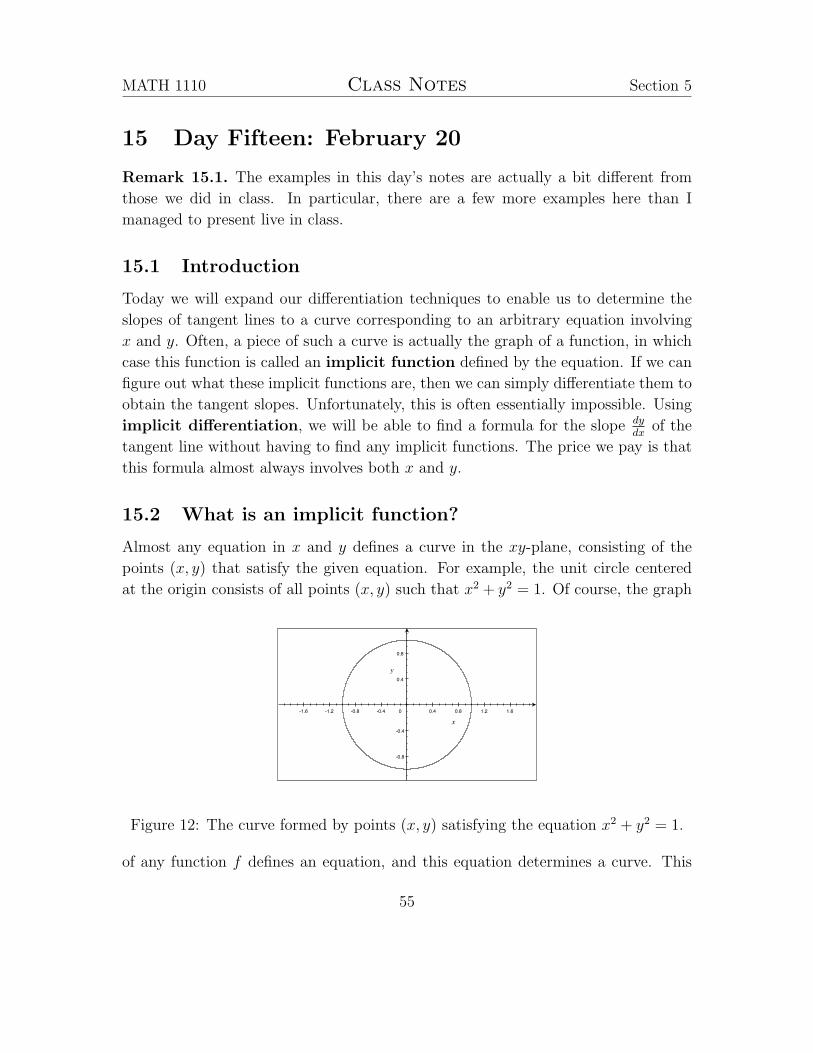
Almost any equation in x and y defines a curve in the xy-plane, consisting of the

points (x, y) that satisfy the given equation. For example, the unit circle centered

at the origin consists of all points (x, y) such that x2 + y2 = 1. Of course, the graph

-1.6 -1.2 -0.8 -0.4 0 0.4 0.8 1.2 1.6

-0.8

-0.4

0.4

0.8

Figure 12: The curve formed by points (x, y) satisfying the equation x2 + y2 = 1.

of any function f defines an equation, and this equation determines a curve. This

55


curve is exactly the graph of the function f , by definition. For instance, the function

f(x) = sinx determines the equation y = sinx, and this equation determines the

graph of f in the xy-plane. Most equations, such as x2 + y2 = 1, are not of this

form. However, many times a piece of the curve corresponding to the equation might

be the graph of a function. We can visually recognize this occurrence by checking

whether just that piece of the curve passes the Vertical Line Test.

For the example of the unit circle, clearly the top semicircle is the graph of some

function, as is the bottom semicircle. We know from experience that these pieces of

the curve are given as the graphs of the functions y =√

1− x2 and y = −√

1− x2,

respectively. If we are given a formula for a function f , how can we check whether

its graph fits in the curve corresponding to a particular equation without having to

draw any pictures?

For convenience, notice that any equation in x and y can be rewritten in the form

F (x, y) = 0 for some function F (x, y) of two variables. For example, the equation

y2 = x can be written as

F (x, y) = 0, where F (x, y) = y2 − x,

and the equation x2 + y2 = 1 can be written as

G(x, y) = 0, where G(x, y) = x2 + y2 − 1.

Definition 15.2. A function y = f(x) is implicitly defined by the equation

F (x, y) = 0 if

F(a, f(a)

)= 0

for all a in the domain of f . This means exactly that every point (x, y) =(x, f(x)

)on the graph of y = f(x) is a solution of the equation F (x, y) = 0. We sometimes

say that f is an implicit function defined by the equation F (x, y) = 0.

Example 15.3.

1. Consider the equation y2 = x from last class. We can write this as F (x, y) = 0,

where F (x, y) = y2 − x. We noted previously that the graphs of the functions

f1(x) =√x and f2(x) = −

√x are all contained in the curve corresponding to

y2 = x. Observe that f1 and f2 are indeed implicitly defined by this equation,

because

F(x, f1(x)

)= F

(x,√x)

= (√x)2 − x = x− x = 0

56


and

F(x, f2(x)

)= F

(x,−√x)

= (−√x)2 − x = x− x = 0.

2. Let G(x, y) = x2 − y2 − 1, so that the equation G(x, y) = 0 describes the unit

circle centered at the origin. Let g1(x) =√

1− x2 and g2(x) = −√

1− x2.

Then

G(x, g1(x)

)= G

(x,√

1− x2)

= x2 + (√

1− x2)2 − 1 = x2 + 1− x2 − 1 = 0

and

G(x, g2(x)

)= G

(x,−√

1− x2)

= x2 + (−√

1− x2)2− 1 = x2 + 1− x2− 1 = 0.

Clearly, the easiest way to get an implicit function out of an equation is to solve

that equation for y. This is exactly how one obtains f1 and f2 from F (x, y) = 0 and

g1 and g2 from G(x, y) = 0 in the previous example. Unfortunately, it is not hard

at all to come up with an equation which cannot easily be solved for y, but which

nonetheless determines a curve that obviously has pieces that are the graphs of some

functions. See Figure 13, for instance.

-5 -4 -3 -2 -1 0 1 2 3 4 5

-2

-1

1

2

Figure 13: The curve corresponding to the equation xy3 − y2 + 2x2 = 0. Certain

pieces of this curve must be the graphs of some functions, but it is unclear what

these functions are.

In this class, we have learned how to use information about the slopes of the

tangent lines to curves to study those curves. So far, we only really know how to

determine the slope of a tangent line to the graph of a function. When a piece of a

57


curve can be represented as the graph of a function, we can determine the slope of

tangent lines to that piece by differentiating the function. But as we saw, it is not

always easy, or indeed even possible, to figure out what the implicit function is! But

by a minor miracle, we can essentially calculate the derivative of the implicit function

without having to know what it is! This process is called implicit differentiation.

15.3 Implicit differentiation

Beginning with an equation, such as y2 = x, the process of finding a formula for

the slopes of tangent lines to the curve represented by this equation, which we call

implicit differentiation, proceeds in two relatively easy steps.

Step 1. Differentiate both sides of the equation with respect to x (i.e. take ddx

of

each side and set the results equal to each other), treating y as a function of x.

For example, if y is a function of x, then ddxy = dy

dx, so by the Chain Rule we

haved

dxy2 = 2y

(d

dxy

)= 2y

dy

dx.

(Sometimes we write y′ for dydx

, to save labour.) So the equation y2 = x leads

to the following equations.

y2 = x

d

dxy2 =

d

dxx

2ydy

dx= 1

Step 2. Solve for dydx

= y′.

In our example, we have 2y dydx

= 1, so

dy

dx=

1

2y.

Remark 15.4. You probably noticed that the result of implicit differentiation is a

formula for dydx

in terms of both x and y. In theory, if y really is a function of x, then

58


this formula for dydx

really only depends on x, but that relies on our being able to

figure out a formula for the implicit function y as a function of x. To avoid doing

this, we pay the price of having to a formula involving both x and y, but it is a small

price to pay in most situations.

Example 15.5.

Above, we found that for the curve represented by the equation y2 = x, we havedydx

= 12y

. Let’s check this formula.

Suppose we want the slope of the tangent line to y2 = x at the point (4, 2), noting

that this point actually is on this curve. This point lies on the portion of the curve

that is given as the graph of the function f(x) =√x, so the slope of the tangent

when x = 4 is

f ′(4) = f ′(x)|x=4 =1

2√x

∣∣∣∣x=4

=1

2√

4=

1

4.

Using our result from implicit differentiation, we have

dy

dx

∣∣∣∣(x,y)=(4,2)

=1

2y

∣∣∣∣(x,y)=(4,2)

=1

2 · 2=

1

4.

Our answers match!

It is not too hard to verify that this will happen for any x in the domain of

f(x) =√x. Note that

dy

dx

∣∣∣∣(x,y)=

(x,f(x)

) =1

2y

∣∣∣∣(x,y)=(x,

√x)

=1

2√x

= f ′(x).

Example 15.6.

1. Question: Find the slope of the circle x2 + y2 = 25 at the point (−3, 4).

Answer: First note that this point actually is on the circle, because (−3)2 +

42 = 9+16 = 25. We could do this problem by using the implicit function

y =√

1− x2, but that would involve differentiating a square root and a

59


pesky Chain Rule. Implicit differentiation is easier.

x2 + y2 = 25d

dx(x2 + y2) =

d

dx(25)

2x+ 2ydy

dx= 0

2ydy

dx= −2x

dy

dx= −2x

2y= −x

y

Thereforedy

dx

∣∣∣∣(x,y)=(−3,4)

= −xy

∣∣∣∣(x,y)=(−3,4)

= −−3

4=

3

4.

2. Question: Find dydx

if y sinx = x3 + cos y.

Answer: Here we do not even have the option of solving for y to find an

implicit function. We have to use implicit differentiation.

y sinx = x3 + cos yd

dx(y sinx) =

d

dx

(x3 + cos y

)dy

dx· sinx+ y cosx = 3x2 − sin y

dy

dx

sinxdy

dx+ cos y

dy

dx= 3x2 − y cosx

(sinx+ cos y)dy

dx= 3x2 − y cosx

dy

dx=

3x2 − y cosx

sinx+ cos y

Notice how we used the Product Rule to compute ddx

(y sinx).

3. Question: Find an equation of the line tangent to the curve x2 +xy+2y3 = 4

at the point (−2, 1).

Answer: Note that this point is indeed on the curve, since (−2)2 + (−2)(1) +

2(1)3 = 4− 2 + 2 = 4. Taking ddx

of each side of the equation, we have the

60


following.

2x+ y + xdy

dx+ 6y2 dy

dx= 0

(x+ 6y2)dy

dx= −(2x+ y)

dy

dx= − 2x+ y

x+ 6y2

Thereforedy

dx

∣∣∣∣(x,y)=(−2,1)

= − 2(−2) + 1

−2 + 6(1)2= −−3

4=

3

4.

Therefore this tangent line has slope 34

and contains the point (−2, 1), so

it is given by the equation

y − 1 =3

4(x+ 2) or y =

3

4x+

5

2.

4. Question: For any constants a and b, the equations x2 − y2 = a and xy = b

represent hyperbolas. Show that they intersect at right angles, i.e. that

at any point where the curves intersect, their tangent lines are perpendic-

ular.

Answer: The tangent slope to the curve x2 − y2 = a is given by the equation

2x − 2y dydx

= 0, so dydx

= xy. The tangent slope to xy = b is given by

y + x dydx

= 0, so dydx

= − yx.

Suppose the two curves intersect at the point (x0, y0). The tangent slopes

at this point are x0

y0and − y0

x0. Since

x0

y0

· −y0

x0

= −1,

the tangent lines at this point are perpendicular to each other.

We can also use implicit differentiation to calculate higher derivatives of y with

respect to x, although this can get messy very quickly.

Example 15.7.

1. Question: If xy + y2 = 2x, what is y′′?

61


Answer: First we calculate y′.

y + xy′ + 2yy′ = 2

y′(x+ 2y) = 2− y

y′ =2− yx+ 2y

Just as y′ = ddxy, note that y′′ = d

dxy′. Therefore

y′′ =d

dxy′

=d

dx

2− yx+ 2y

=(x+ 2y) · d

dx(2− y)− (2− y) · d

dx(x+ 2y)

(x+ 2y)2

=(x+ 2y)(2− y′)− (2− y)(1 + 2y′)

(x+ 2y)2.

This might seem to be the best we can do, but notice that this is a

formula for y′′ involving three quantities : x, y, and y′. But we already

have a formula for y′ in terms of x and y, so let’s use it! Our final formula

for y′′ is

y′′ =(x+ 2y)(2− y′)− (2− y)(1 + 2y′)

(x+ 2y)2

=(x+ 2y)

(2− 2−y

x+2y

)− (2− y)

(1 + 2 · 2−y

x+2y

)(x+ 2y)2

.

This formula is a little messy, but unless there is any particular reason to

simplify it, we can just leave it as it is.

2. Question: Find d2ydx2 if x2 + xy + 2y3 = 4.

Answer: We calculated in part 3. of Example 15.5 that

dy

dx= − 2x+ y

x+ 6y2.

62


Therefore

d2y

dx2=

d

dx

(− 2x+ y

x+ 6y2

)= −

(x+ 6y2)(2 + dy

dx

)− (2x+ y)

(1 + 12y dy

dx

)(x+ 6y2)2

= −(x+ 6y2)

(2− 2x+y

x+6y2

)− (2x+ y)

(1− 12y · 2x+y

x+6y2

)(x+ 6y2)2

.

63

Class Notes for Math 1110, Section 5 - Cornell Universitygoldberg/ClassNotes.pdfClass Notes for Math...

Documents

Transcript of Class Notes for Math 1110, Section 5 - Cornell Universitygoldberg/ClassNotes.pdfClass Notes for Math...