Class 6: Tuesday, Sep. 28

• Section 2.4.

• Checking the assumptions of the simple linear regression model:– Residual plots– Normal quantile plots

• Outliers and influential observations

Checking the model• The simple linear regression model is a great tool

but its answers will only be useful if it is the right model for the data. We need to check the assumptions before using the model.

• Assumptions of the simple linear regression model:1. Linearity: The mean of Y|X is a straight line.2. Constant variance: The standard deviation of Y|X is

constant.3. Normality: The distribution of Y|X is normal.4. Independence: The observations are independent.

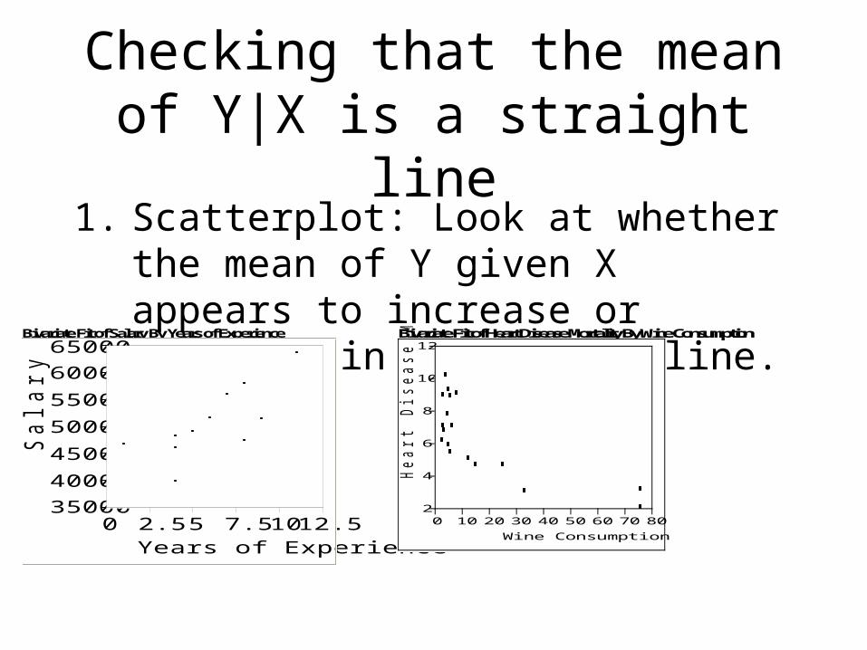
Checking that the mean of Y|X is a straight line

1. Scatterplot: Look at whether the mean of Y given X appears to increase or decrease in a straight line.

Bivariate Fit of Salary By Years of Experience

35000

40000

45000

50000

55000

60000

65000

Sa

lary

0 2.5 5 7.5 1012.5Years of Experience

Bivariate Fit of Heart Disease Mortality By Wine Consumption

2

4

6

8

10

12

He

art

Dis

ea

se

Mo

rta

lity

0 10 20 30 40 50 60 70 80

Wine Consumption

Residual Plot• Residuals: Prediction error of using

regression to predict Yi for observation i:

, where

• Residual plot: Plot with residuals on the y axis and the explanatory variable (or some other variable) on the x axis.

ii XY 10ˆˆˆ iii YYres ˆ

-3-2-10123

Res

idua

l

0 10 20 30 40 50 60 70 80

Wine Consumption

-10000

-5000

0

5000

Resid

ual

0 2.5 5 7.5 10 12.5

Years of Experience

• Residual Plot in JMP: After doing Fit Line, click red triangle next to Linear Fit and then click Plot Residuals.

• What should the residual plot look like if the simple linear regression model holds? Under simple linear regression model, the residuals

should have approximately a normal distribution with mean zero and a standard deviation which is the same for all X.

• Simple linear regression model: Residuals should appear as a “swarm” of randomly scattered points about zero. Ideally, you should not be able to detect any patterns. (Try not to read too much into these plots – you’re looking for gross departures from a random scatter).

• A pattern in the residual plot that for a certain range of X the residuals tend to be greater than zero or tend to be less than zero indicates that the mean of Y|X is not a straight line.

)ˆˆ(ˆ10 iiiii XYYYres

B i v a r i a t e F i t o f M i l e a g e B y S p e e d

5

10

15

20

25

30

35

40Mil

eage

0 10 20 30 40 50 60 70 80 90 100 110

Speed

Linear Fit

L i n e a r F i t M i l e a g e = 2 3 . 2 6 6 7 7 6 - 0 . 0 0 1 2 7 0 1 S p e e d

-20

-10

0

10

Resid

ual

0 10 20 30 40 50 60 70 80 90 100 110

Speed

D a t a S i m u l a t e d F r o m A S i m p l e L i n e a r R e g r e s s i o n M o d e l I d e a l r e g . J M P B i v a r i a t e F i t o f Y B y X

0

10

20

30

40

50

60

70

80

90

100

110

Y

0 10 20 30 40 50 60 70 80 90 100 110

X

-2

-1

0

1

2

Resid

ual

0 10 20 30 40 50 60 70 80 90 100 110

X

Checking Constant Variance

• Use residual plot of residuals vs. X to check constant variance assumption.

• Constant variance: Spread of residuals is similar for all ranges of X

• Nonconstant variance: Spread of residuals is different for different ranges of X.

– Fan shaped plot: Residuals are increasing in spread as X increases

– Horn shaped plot: Residuals are decreasing in spread as X increases.

D a t a S i m u l a t e d F r o m A S i m p l e L i n e a r R e g r e s s i o n M o d e l I d e a l r e g . J M P B i v a r i a t e F i t o f Y B y X

0

10

20

30

40

50

60

70

80

90

100

110

Y

0 10 20 30 40 50 60 70 80 90 100 110

X

-2

-1

0

1

2

Resid

ual

0 10 20 30 40 50 60 70 80 90 100 110

X

S i m u l a t e d D a t a f r o m a M o d e l w i t h N o n c o n s t a n t V a r i a n c e B i v a r i a t e F i t o f Y B y X

-100

-50

0

50

100

150

200

250

300

350

Y

0 10 20 30 40 50 60 70 80 90 100 110

X

-200

-100

0

100

200

300

Resid

ual

0 10 20 30 40 50 60 70 80 90 100 110

X

Name Game Bivariate Fit of Proportion recalled By Position

0

0.1

0.2

0.3

0.4

0.5

0.6

0.7

0.8

0.9

1

1.1

Pro

port

ion r

ecalled

1 2 3 4 5 6 7 8 9 10

Position

-0.8

-0.5

-0.2

0.1

0.4

Res

idua

l

1 2 3 4 5 6 7 8 9 10

Position

Checking Normality

• If the distribution of Y|X is normal, then the residuals should have approximately a normal distribution.

• To check normality, make histogram and normal quantile plot of residuals.

• In JMP, after using Fit Line, click red triangle next to Linear Fit and click save residuals. Click Analyze, Distribution, put Residuals in Y, click OK and then after histogram appears, click red triangle next to Residuals and click Normal Quantile Plot.

Name Game Distributions Residuals Proportion recalled

-0.7

-0.6

-0.5

-0.4

-0.3

-0.2

-0.1

0

0.1

0.2

0.3

0.4.01 .05.10 .25 .50 .75 .90.95 .99

-3 -2 -1 0 1 2 3

Normal Quantile Plot

Simulation from Simple Linear Regression Model Distributions Residuals Y

-3

-2

-1

0

1

2

3.01 .05.10 .25 .50 .75 .90.95 .99

-3 -2 -1 0 1 2 3

Normal Quantile Plot

Normal Quantile Plot• Section 1.3.• Most useful tool for assessing normality.• Plot of residuals (or whatever variable is being checked

for normality) on y-axis versus z-score of percentile of data point.

• If the true distribution is normal, the normal quantile plot will be a straight line. Deviations from a straight line indicate that the distribution is not normal.

• The dotted red lines are “confidence bands.” If all the points lie inside the confidence bands, then we feel that the normality assumption is reasonable.

Independence• In a problem where the data is collected over time, plot the

residuals vs. time. • For simple linear regression model, there should be no

pattern in residuals over time.• Pattern in residuals over time where residuals are higher or

lower in early part of data than later part of data indicates that relationship between Y and X is changing over time and might indicate that there is a lurking variable.

• Lurking variable: A variable that is not among the explanatory or response variables in a study and yet may influence the interpretation of relationships among those variables.

Residual vs. Time Example

• Mathematics dept. at large state university must plan number of instructors required for large elementary courses and wants to predict enrollment in elementary math courses (y) based on number of first-year students (x).

• Data in mathenroll.JMP• Residual plot vs. time in JMP: After fit y by x, fit

line, click red triangle next to linear fit and click save residuals. Then use fit y by x with y = residuals and x = year.

Residual Plots

-200

0

200

400R

esi

du

al

3750 4000 4250 4500 4750 5000First year students

-200

-100

0

100

200

300

400

Re

sid

ua

ls M

ath

en

rollm

en

t

1992 1996 1998 2000Year

Analysis of Math Enrollment

• Residual plot versus time order indicates that there must be a lurking variable associated with time, in particular there is a change in the relationship between y and x between 1997 and 1998.

• In fact, one of schools in the university changed its program to require that entering students take another mathematics course beginning in 1998, increasing enrollment.

• Implication: Data from before 1998 should not be used to predict future math enrollment.

What to Do About Violations of Simple Linear Regression Model• Coming up in the Future:• Nonlinearity: Transformations (Chapter 2.6),

Polynomial Regression (Chapter 11)• Nonconstant Variance: Transformations (Chapter

2.6)• Nonnormality: Transformations (Chapter 2.6).• Lack of independence: Incorporate time into

multiple regression (Chapter 11), time series techniques (Stat 202).

Outliers and Influential Observations

• Outlier: Any really unusual observation.• Outlier in the X direction (called high leverage point):

Has the potential to influence the regression line.• Outlier in the direction of the scatterplot: An

observation that deviates from the overall pattern of relationship between Y and X. Typically has a residual that is large in absolute value.

• Influential observation: Point that if it is removed would markedly change the statistical analysis. For simple linear regression, points that are outliers in the x direction are often influential.

Housing Prices and Crime Rates• A community in the Philadelphia area is interested in

how crime rates are associated with property values. If low crime rates increase property values, the community might be able to cover the costs of increased police protection by gains in tax revenues from higher property values.

• The town council looked at a recent issue of Philadelphia Magazine (April 1996) and found data for itself and 109 other communities in Pennsylvania near Philadelphia. Data is in philacrimerate.JMP. House price = Average house price for sales during most recent year, Crime Rate=Rate of crimes per 1000 population.

Bivariate Fit of HousePrice By CrimeRate

0

100000

200000

300000

400000

500000

Ho

us

eP

ric

e

GladwyneHaverford

Phila, N

Phila,CC

0 50 100 150 200 250 300 350 400

CrimeRate

Center City Philadelphia is a high leverage point. Gladwyne and Haverford are outliers in the direction of the scatterplot (their house price) is considerably higher than one would expect given their crime rate.

Which points are influential?B iv a r i a t e F i t o f H o u s e P r ic e B y C r im e R a t e

0

1 0 0 0 0 0

2 0 0 0 0 0

3 0 0 0 0 0

4 0 0 0 0 0

5 0 0 0 0 0

Ho

us

eP

rice

G la d w y n eH a v e rfo rd

P h ila , N

P h ila ,C C

0 5 0 1 0 0 1 5 0 2 0 0 2 5 0 3 0 0 3 5 0 4 0 0

C rime R a te

L in e a r F it

L in e a r F it

L in e a r F it

A l l o b s e r v a t i o n s L i n e a r F i t H o u s e P r ic e = 1 7 6 6 2 9 .4 1 - 5 7 6 . 9 0 8 1 3 C r im e R a te

W i t h o u t C e n t e r C i t y P h i l a d e l p h i a L i n e a r F i t H o u s e P r ic e = 2 2 5 2 3 3 .5 5 - 2 2 8 8 . 6 8 9 4 C r im e R a te

W i t h o u t G l a d w y n e L i n e a r F i t H o u s e P r ic e = 1 7 3 1 1 6 . 4 3 - 5 6 7 . 7 4 5 0 8 C r im e R a te

Center City Philadelphia is influential; Gladwyne is not. In general, points that have high leverage are more likely to be influential.

Formal measures of leverage and influence

• Leverage: “Hat values” (JMP calls them hats)• Influence: Cook’s Distance (JMP calls them Cook’s D

Influence).• To obtain them in JMP, click Analyze, Fit Model, put Y

variable in Y and X variable in Model Effects box. Click Run Model box. After model is fit, click red triangle next to Response. Click Save Columns and then Click Hats for Leverages and Click Cook’s D Influences for Cook’s Distances.

• To sort observations in terms of Cook’s Distance or Leverage, click Tables, Sort and then put variable you want to sort by in By box.

Distributions Cook's D Influence HousePrice

HaverfordGladwyne Phila,CC

0 5 1015202530

h HousePrice

Phila,CC

0 .1.2.3.4.5.6.7.8.9

Center City Philadelphia has both influence (Cook’s Distance much Greater than 1 and high leverage (hat value > 3*2/99=0.06). No otherobservations have high influence or high leverage.

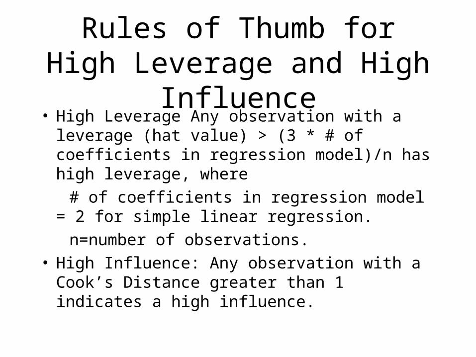
Rules of Thumb for High Leverage and High Influence

• High Leverage Any observation with a leverage (hat value) > (3 * # of coefficients in regression model)/n has high leverage, where

# of coefficients in regression model = 2 for simple linear regression.

n=number of observations. • High Influence: Any observation with a Cook’s

Distance greater than 1 indicates a high influence.

What to Do About Suspected Influential Observations?

See flowchart handout.

Does removing the observation change the

substantive conclusions?• If not, can say something like “Observation x

has high influence relative to all other observations but we tried refitting the regression without Observation x and our main conclusions didn’t change.”

• If removing the observation does change substantive conclusions, is there any reason to believe the observation belongs to a population other than the one under investigation?– If yes, omit the observation and proceed.– If no, does the observation have high leverage (outlier in explanatory

variable).• If yes, omit the observation and proceed. Report that conclusions only apply to a

limited range of the explanatory variable.• If no, not much can be said. More data (or clarification of the influential observation)

are needed to resolve the questions.

• General principle: Delete observations from the analysis sparingly – only when there is good cause (does not belong to population being investigated or is a point with high leverage). If you do delete observations from the analysis, you should state clearly which observations were deleted and why.

Summary• Before using the simple linear regression model, we need to

check its assumptions. Check linearity, constant variance, normality and independence by using scatterplot, residual plot and normal quantile plot.

• Influential observations: observations that, if removed, would have a large influence on the fitted regression model. Examine influential observations, remove them only with cause (belongs to a different population than being studied, has high leverage) and explain why you deleted them.

• Next class: Lurking variables, causation (Sections 2.4, 2.5).