CIVIL ENGINEERING STUDIES UILU-ENG-2007-2009
100
HMA DYNAMIC MODULUS - TEMPERATURE RELATIONS By Gabriel Garcia University of Illinois at Urbana-Champaign and Marshall Thompson University of Illinois at Urbana-Champaign Research Report FHWA-ICT-07-006 A report of the findings of ICT-R39 Validation of Extended Life HMA Design Concepts Illinois Center for Transportation April 2007 CIVIL ENGINEERING STUDIES Illinois Center for Transportation Series No. 07-006 UILU-ENG-2007-2022 ISSN: 0197-9191
Transcript of CIVIL ENGINEERING STUDIES UILU-ENG-2007-2009

HMA DYNAMIC MODULUS - TEMPERATURE RELATIONS
By
Gabriel Garcia University of Illinois at Urbana-Champaign
and
Marshall Thompson
University of Illinois at Urbana-Champaign
Research Report FHWA-ICT-07-006
A report of the findings of
ICT-R39 Validation of Extended Life HMA Design Concepts
Illinois Center for Transportation April 2007
CIVIL ENGINEERING STUDIES Illinois Center for Transportation Series No. 07-006
UILU-ENG-2007-2022 ISSN: 0197-9191

Technical Report Documentation Page
1. Report No. FHWA-ICT-07-006
2. Government Accession No. 3. Recipient's Catalog No.
4. Title and Subtitle HMA DYNAMIC MODULUS – TEMPERATURE RELATIONS
5. Report Date
April, 2007
6. Performing Organization Code
8. Performing Organization Report N o. 7. Author(s) Gabriel Garcia & Marshall Thompson
FHWA-ICT-07-006 UILU-ENG-2007-2022
9. Performing Organization Name and Address Illinois Center for Transportation Department of Civil and Environmental Engineering University of Illinois 205 North Mathews – MC-250 Urbana, IL 61801
10. Work Unit ( TRAIS)
11. Contract or Grant No. ICT-R39
13. Type of Report and Period Covered
Project Report 2002-2006
12. Sponsoring Agency Name and Address Illinois Department of Transportation Bureau of Materials and Physical Research
126 East Ash Street Springfield, IL 62704-4766
14. Sponsoring Agency Code
15. Supplementary Notes
Study was conducted in cooperation with the U.S. Department of Transportation, Federal Highway Administration. 16. Abstract A three-stage study to evaluate Hot Mix Asphalt (HMA) dynamic modulus (E*) predictive models using typical Illinois Department of Transportation (IDOT) mixtures and binders was conducted with the objective to propose HMA modulus-temperature generic relations for pavement design applications. Three E* predictive models were evaluated: the current Witczak model (using different ways to obtain the regression intercept (A) and slope (VTS) of the viscosity temperature susceptibility equation), the new Witczak model, and the Hirsch model. The most promising model was the Hirsch model. This model showed the highest precision and the lowest bias. However in general, the model “under predicted” the E*. Based on the bias found applying the Hirsch model, a set of “Correction Factors” (CF) was determined. After applying the CFs to each group of mixtures, the E* predicted with the Hirsch model showed no appreciable bias. Based on some generic volumetric properties for typical Illinois mixtures and binder G* relations for five Illinois binders, a set of “E*-Temperature generic curves” was developed for five different groups of mixtures, applying the Hirsch model corrected for bias. The generic curves (GCs) for each group of mixtures were compared with the E*-Temperature relations used in the current IDOT full-depth HMA pavement design procedure. In general, the GCs predict much higher HMA E* values for a given temperature and mixture than the current IDOT curves. To verify the applicability of the proposed GCs, five mixtures utilized in the Extended Life HMA Pavement (ELHMAP) project at The Advanced Transportation Research & Engineering Lab (ATREL) were compared against the corresponding GC. The results of this comparison were favorable for 12.5-mm and 19.0-mm mixtures using PG 64-22 and PG 70-22. The result for 12.5-mm SMA using PG 76-28 was not favorable. The proposed GCs are considered reasonable first order estimates of HMA E* for routine pavement design purposes for the mixtures in this study, with the exception of 12.5-mm SMA mixtures. 17. Key Words HMA modulus, hot mix asphalt, HMA modulus-temperature relations
18. Distribution Statement No restrictions. This document is available to the public through the National Technical Information Service, Springfield, Virginia 22161.
19. Security Classif. (of this report) Unclassified
20. Security Classif. (of this page) Unclassified
21. No. of Pages
97 22. Price
Form DOT F 1700.7 (8-72) Reproduction of completed page authorized

ACKNOWLEDGMENTS / DISCLAIMER
This publication is based on the results of Project ICT-R39 “Validation of Design
Principles for Extended Life Hot Mix Asphalt Pavements”. ICT-R39 was conducted in
cooperation with the Illinois Center for Transportation; the Illinois Department of
Transportation; and the U.S. Department of Transportation, Federal Highway
Administration.
Members of the Technical Review Panel are the following: Scott Lackey, David Lippert,
Rick Mauch, Matt Mueller, Paul Niedernhofer, Dave Piper, LaDonna Rowden, Amy
Schutzbach (Chair), Jim Trepanier, Tom Winkelman (all of the Illinois Department of
Transportation) and Hal Wakefield of the Federal Highway Administration .
The contents of this report reflect the views of the authors who are responsible for the
facts and the accuracy of the data presented herein. The contents do not necessarily
reflect the official views or policies of the Illinois Center for Transportation, the Illinois
Department of Transportation, or the Federal Highway Administration. This report does
not constitute a standard, specification or regulation.
i

i
TABLE OF CONTENTS
1. Introduction .............................................................................................................................................1 2. Organization of the Study ......................................................................................................................4 3. Dynamic Modulus Predictive Models Evaluated .................................................................................6
3.1 Current Witczak Predictive Model .......................................................................................................6 3.2 New Witczak Predictive Model ............................................................................................................7 3.3 Hirsch Model........................................................................................................................................9
4. Evaluation Criteria ................................................................................................................................10 5. Mixture MCs and Isochronal Plots ......................................................................................................13 6. Binder MCs and Isochronal Plots........................................................................................................14 7. Results 1st Stage ...................................................................................................................................15 8. Results 2nd Stage...................................................................................................................................19 9. Results 3rd Stage ...................................................................................................................................22 10. E*-Temperature GCs...........................................................................................................................33 11. Application of Proposed GCs ............................................................................................................39 12. Summary and Conclusions................................................................................................................42 13. References...........................................................................................................................................43 APPENDIX A ..............................................................................................................................................46
1. Mixture: 5n70-4 ..................................................................................................................................47 2. Mixture: 6n90-4 ..................................................................................................................................48 3. Mixture: 9n90-4 ..................................................................................................................................49 4. Mixture: 8n105-4 ................................................................................................................................50 5. Mixture: 8n70-4 ..................................................................................................................................51 6. Mixture: 5n90-4 ..................................................................................................................................52 7. Mixture: 3n70-4 ..................................................................................................................................53 8. Mixture: 3n90t-4 .................................................................................................................................54 9. Mixture: 6n50-4 ..................................................................................................................................55 10. Mixture: 1n105-4 ..............................................................................................................................56 11. Mixture: 2n90-4 ................................................................................................................................57 12. Mixture: 3n90-4 ................................................................................................................................58 13. Mixture: 5n105-4 ..............................................................................................................................59 14. Mixture: 6n50s-4 ..............................................................................................................................60 15. Mixture: 1n80d-4 ..............................................................................................................................61 16. Mixture: 1n80s-4 ..............................................................................................................................62
APPENDIX B ..............................................................................................................................................63 1. Binder: B1 (SBS 70-22) .....................................................................................................................64 2. Binder: B2 (64-22)..............................................................................................................................65 3. Binder: B3 (64-22)..............................................................................................................................66 4. Binder: B4 (SBS 76-28) .....................................................................................................................67 5. Binder: B5 (SBS 76-22) .....................................................................................................................68
APPENDIX C ..............................................................................................................................................69 1. Model: Current Witczak (1) ...............................................................................................................70 2. Model: Current Witczak (2) ...............................................................................................................72 3. Model: Current Witczak (3) ...............................................................................................................74 4. Model: New Witczak ..........................................................................................................................75

ii
5. Model: Hirsch.....................................................................................................................................77 APPENDIX D ..............................................................................................................................................79
1. Model: Current Witczak (1) ...............................................................................................................80 2. Model: Hirsch.....................................................................................................................................83
APPENDIX E ..............................................................................................................................................86 1. Mixture: 1111......................................................................................................................................87 2. Mixture: 1112......................................................................................................................................88 3. Mixture: 1113......................................................................................................................................89 4. Mixture: 1114......................................................................................................................................90 5. Mixture: 3809......................................................................................................................................91

iii
LIST OF TABLES
Table 1. Characteristic Frequency of some Recognized Design Procedures. .............................................3 Table 2. Typical IDOT Mixtures, UIUC Study. ..............................................................................................4 Table 3. Typical IDOT Binders, NCSC Data. ................................................................................................4 Table 4. Mixtures Evaluated in the 2nd Stage................................................................................................5 Table 5. Statistics for Current Witczak Dynamic Modulus Predictive Equation............................................7 Table 6. Statistics for New Witczak Predictive Model...................................................................................9 Table 7. Comparison of E* Predictive Models [Modified from Bari and Witczak, 2006]. ..............................9 Table 8. Summary of the Database used in the Development of the Hirsch Model. ..................................10 Table 9. Mixtures Selected 1st Stage. .........................................................................................................15 Table 10. Results of Precision and Bias, 1st Stage.....................................................................................18 Table 11. Rank of Models Based on Results of Precision at Mixture Level, 1st Stage...............................18 Table 12. Rank of Models Based on Results of Bias at Mixture Level, 1st Stage.......................................18 Table 13. Rank of Models Based on Results of Precision and Bias at Global Level, 1st Stage. ................18 Table 14. Mixtures Selected 2nd Stage. ......................................................................................................19 Table 15. Results of Precision and Bias, 2nd Stage. ...................................................................................22 Table 16. Groups of Mixtures for 3rd Stage Analysis. .................................................................................23 Table 17. Hirsch Model Bias CFs for each Group of Mixtures....................................................................27 Table 18. Generic Properties for each Group of Mixtures. .........................................................................33 Table 19. Polynomial Representation of GCs @10Hz, for each Group of Mixtures...................................36 Table 20. Comparison of E* for 12.5-mm vs. 19.0-mm Mixtures................................................................36 Table 21. E*-Temperature GCs @ 10Hz Proposed in this Study...............................................................37 Table 22. Mixtures Utilized in ELHMAP Project at ATREL. ........................................................................39 Table 23. E* from ATREL Mixtures MCs vs. E* from Corresponding GC. .................................................41

iv
LIST OF FIGURES
Figure 1. EHMA-Temperature Relations for Typical IDOT Class I Mixture [Thompson and Cation, 1986]. ...2 Figure 2. Design Pavement HMA Temperature [IDOT, 2002]. .....................................................................3 Figure 3. Concepts of Precision and Bias...................................................................................................11 Figure 4. Example of Correction of Bias. ....................................................................................................12 Figure 5. Example of a Well-Fitted MC. ......................................................................................................13 Figure 6. Example of a Poorly-Fitted MC....................................................................................................14 Figure 7. Range of Frequency where Binder and Mixture MC Overlap......................................................15 Figure 8. Results for Mixture 3n90-4 Applying Current Witczak (1) Model.................................................16 Figure 9. Results for All Mixtures, Applying Current Witczak (1) Model. ....................................................16 Figure 10. Results of Precision and Bias, 1st Stage....................................................................................17 Figure 11. Results for Mixture 5n70-4 Applying Hirsch Model....................................................................20 Figure 12. Results for All Mixtures, Applying Hirsch Model. .......................................................................21 Figure 13. Results of Precision and Bias, 2nd Stage...................................................................................21 Figure 14. Range of Temperatures, Mixtures and Binders Before Extrapolation. ......................................24 Figure 15. Range of Temperatures, Mixtures and Binders After Extrapolation. .........................................24 Figure 16. Effect of Binder Inside the Range Studied.................................................................................25 Figure 17. Isochronal Plots from Lab Data for Every Group of Mixtures (@ 10 Hz). .................................26 Figure 18. Results for Every Group of Mixtures..........................................................................................28 Figure 19. Results for All Groups of Mixtures Consolidated. ......................................................................29 Figure 20. Distribution of Errors, All Groups of Mixtures Consolidated. .....................................................29 Figure 21. Isochronal Plots for Group of Mixtures After Applying CF to Hirsch E* Predictions..................31 Figure 22. Results for All Groups of Mixtures Consolidated, After Correction............................................32 Figure 23. Distribution of Errors, All Groups of Mixtures Consolidated, After Correction...........................32 Figure 24. GCs for 9.5-mm Mixtures @ 10Hz. ...........................................................................................34 Figure 25. GCs for 12.5-mm Mixtures @ 10Hz. .........................................................................................34 Figure 26. GCs for 19.0-mm Mixtures @ 10Hz. .........................................................................................35 Figure 27. GCs for 12.5-mm-SMA Mixture @ 10Hz. ..................................................................................35 Figure 28. GCs Proposed for 9.5-mm Mixtures @ 10Hz. ...........................................................................37 Figure 29. GCs Proposed for 12.5-mm & 19.0-mm Mixtures @ 10Hz. ......................................................38 Figure 30. GCs Proposed for 19.0-mm Mixtures (PG 76-28) @ 10Hz. ......................................................38 Figure 31. GCs Proposed for 12.5-mm-SMA Mixtures @ 10Hz.................................................................39 Figure 32. GC 12.5-mm&19.0-mm (PG 64-22) Mixtures vs. Lab Data Curves, Mixtures 1112 and 1114 @ 10Hz. ...........................................................................................................................................................40 Figure 33. GC 12.5-mm&19.0-mm (PG 70-22) Mixtures vs. Lab Data Curves, Mixtures 1111 and 1113 @ 10Hz. ...........................................................................................................................................................40 Figure 34. GC 12.5-mm-SMA (PG 76-28) Mixtures vs. Lab Data Curves for Mixture 3809 @ 10Hz.........41

v
EXECUTIVE SUMMARY
A three-stage study to evaluate Hot Mix Asphalt (HMA) dynamic modulus (E*) predictive models using typical Illinois Department of Transportation (IDOT) mixtures and binders was conducted with the objective to propose HMA modulus-temperature generic relations for pavement design applications. Three E* predictive models were evaluated: the current Witczak model (using different ways to obtain the regression intercept (A) and slope (VTS) of the viscosity temperature susceptibility equation), the new Witczak model, and the Hirsch model. The most promising model was the Hirsch model. This model showed the highest precision and the lowest bias. However in general, the model “under predicted” the E*. Based on the bias found applying the Hirsch model, a set of “Correction Factors” (CF) was determined. After applying the CFs to each group of mixtures, the E* predicted with the Hirsch model showed no appreciable bias. Based on some generic volumetric properties for typical Illinois mixtures and binder G* relations for five Illinois binders, a set of “E*-Temperature generic curves” was developed for five different groups of mixtures, applying the Hirsch model corrected by bias. The generic curves (GCs) for each group of mixtures were compared with the E*-Temperature relations used in the current IDOT full-depth HMA pavement design procedure. In general, the GCs predict much higher HMA E* values for a given temperature and mixture than the current IDOT curves. To verify the applicability of the proposed GCs, five mixtures utilized in the Extended Life HMA Pavement (ELHMAP) project at Advanced Transportation Research & Engineering Lab (ATREL) were compared against the corresponding GC. The results of this comparison were favorable for 12.5-mm and 19.0-mm mixtures using PG 64-22 and PG 70-22. The result for 12.5-mm SMA using PG 76-28 was not favorable. The proposed GCs are considered reasonable first order estimates of HMA E* for routine pavement design purposes for the mixtures in this study, with the exception of 12.5-mm SMA mixtures.
1
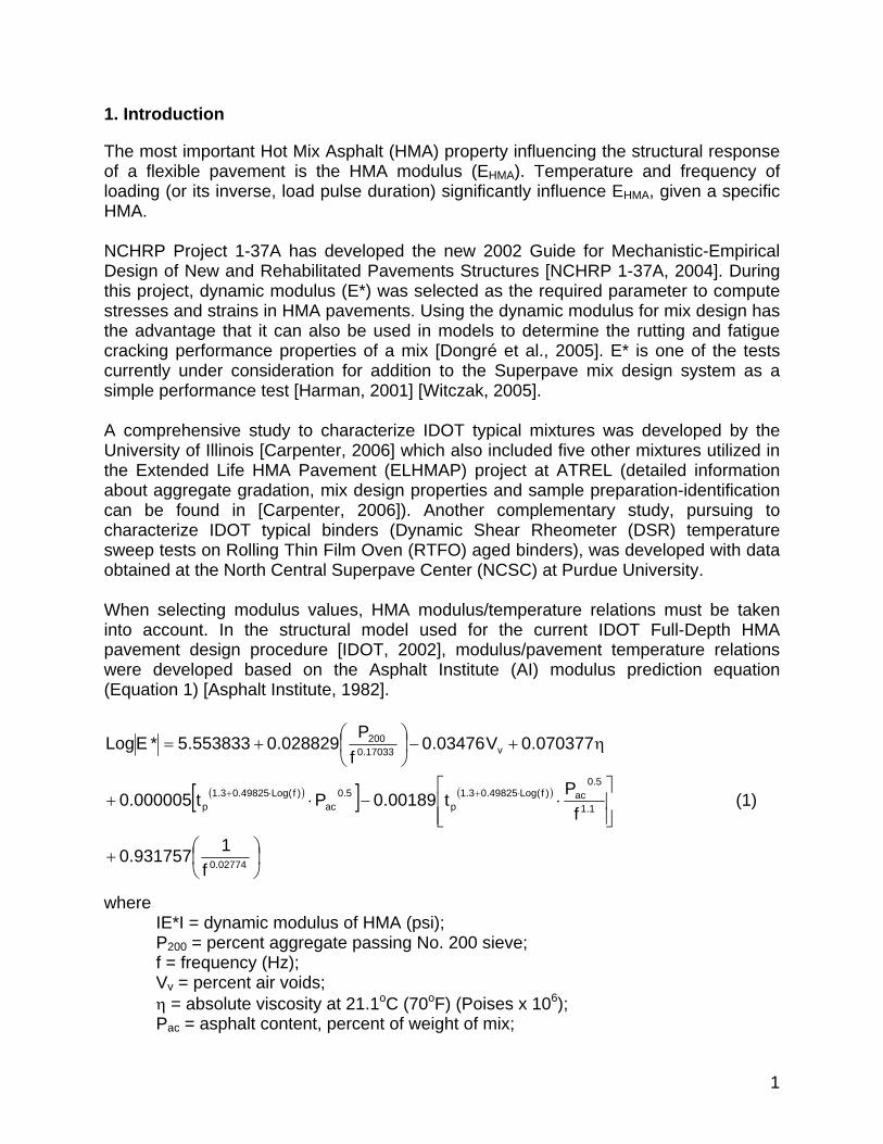
1. Introduction
The most important Hot Mix Asphalt (HMA) property influencing the structural response of a flexible pavement is the HMA modulus (EHMA). Temperature and frequency of loading (or its inverse, load pulse duration) significantly influence EHMA, given a specific HMA. NCHRP Project 1-37A has developed the new 2002 Guide for Mechanistic-Empirical Design of New and Rehabilitated Pavements Structures [NCHRP 1-37A, 2004]. During this project, dynamic modulus (E*) was selected as the required parameter to compute stresses and strains in HMA pavements. Using the dynamic modulus for mix design has the advantage that it can also be used in models to determine the rutting and fatigue cracking performance properties of a mix [Dongré et al., 2005]. E* is one of the tests currently under consideration for addition to the Superpave mix design system as a simple performance test [Harman, 2001] [Witczak, 2005]. A comprehensive study to characterize IDOT typical mixtures was developed by the University of Illinois [Carpenter, 2006] which also included five other mixtures utilized in the Extended Life HMA Pavement (ELHMAP) project at ATREL (detailed information about aggregate gradation, mix design properties and sample preparation-identification can be found in [Carpenter, 2006]). Another complementary study, pursuing to characterize IDOT typical binders (Dynamic Shear Rheometer (DSR) temperature sweep tests on Rolling Thin Film Oven (RTFO) aged binders), was developed with data obtained at the North Central Superpave Center (NCSC) at Purdue University. When selecting modulus values, HMA modulus/temperature relations must be taken into account. In the structural model used for the current IDOT Full-Depth HMA pavement design procedure [IDOT, 2002], modulus/pavement temperature relations were developed based on the Asphalt Institute (AI) modulus prediction equation (Equation 1) [Asphalt Institute, 1982].
( )[ ] ( )
⎟⎠⎞
⎜⎝⎛+
⎥⎥⎦
⎤
⎢⎢⎣
⎡⋅−⋅+
η+−⎟⎠
⎞⎜⎝
⎛+=
⋅+⋅+
02774.0
1.1
5.0ac)f(Log49825.03.1
p5.0
ac)f(Log49825.03.1
p
v17033.0200
f1931757.0
fPt00189.0Pt000005.0
070377.0V03476.0fP028829.0553833.5*ELog
(1)
where IE*I = dynamic modulus of HMA (psi); P200 = percent aggregate passing No. 200 sieve; f = frequency (Hz); Vv = percent air voids; η = absolute viscosity at 21.1oC (70oF) (Poises x 106); Pac = asphalt content, percent of weight of mix;

2
tp = temperature (oF). The AI equation was used to predict EHMA-temperature relations for high-type dense-graded HMA mixes (AC-10 and AC-20 binders), using representative values for absolute viscosity (at 21.1oC (70oF)) for the two different asphalt cement grades (1x10⁶ poises for AC-10, and 2x10⁶ poises for AC-20). The AI equation also requires a frequency as an input. A frequency of 10 Hz was selected because it was found appropriate for the mixed traffic conditions and different pavement thicknesses considered [Thompson and Cation, 1986 and Thompson, 1987]. Other inputs required for the AI equation were established based on representative values found in mixture data from past Illinois HMA construction (asphalt content = 5%, percent passing #200 sieve = 5%, and air voids = 2%). Figure 1 shows the EHMA-temperature relation developed based on the approach described.
Asphalt Content = 5%Air Voids = 2%Passing #200 = 5%Frequency = 10 HzViscosity (Poises x 106) AC-10 = 1 AC-20 = 2
30 40 50 60 70 80 90 100
HMA Temperature, oF
HM
A M
odul
us, k
si
150
200
300
400
500
600
1000
700800900
2000
3000
AC-10
AC-20
Figure 1. EHMA-Temperature Relations for Typical IDOT Class I Mixture [Thompson and Cation,
1986].
The influence of loading frequency on the performance of the HMA layer is similar to the influence of temperature, which means that elastic, plastic, and fatigue behavior are affected [Ullidtz, 1987]. It is important to summarize some recognized design procedure approaches to characterize the effect of the frequency on the EHMA (Table 1), which are in line with the value adopted by IDOT. The United Kingdom (UK) procedure uses a unique frequency of 5 Hz [Thompson, 2005]. The Asphalt Institute procedure is based on a frequency of 10 Hz [Asphalt Institute, 1991]. The Shell Design Method utilizes a constant loading time of 0.02 seconds (equivalent to a frequency of 8 Hz using the Van der Poel relationship) which is representative of the average loading times for commercial vehicles at a speed of 50-60 km/h [Claessen et al., 1977]. In the case of the French design approach they fix minimum values for EHMA at 15oC (59oF) and 10 Hz, but to determine the effect of temperature they perform EHMA tests at 6 temperatures and 10 Hz [LCPC-SETRA, 1997].

3
Table 1. Characteristic Frequency of some Recognized Design Procedures.
The “design pavement HMA mixture temperature” is selected from Figure 2, based on the job location. It establishes the framework to develop any HMA modulus/temperature relation.
Figure 2. Design Pavement HMA Temperature [IDOT, 2002].
The current HMA modulus/temperature relation is based on technology and practices of the 1980’s. Improved technologies concerning materials (aggregate and asphalt binders [PG asphalts, modified asphalts]), HMA mixture design practices [Superpave-based], and HMA property characterization [dynamic modulus and fatigue] are now available and being used in current IDOT HMA policies/practices. Consequently, a study proposing new HMA modulus/temperature relations, in tune with these new technologies, will be presented. These relations will be based on HMA E* predictive models.
Design Procedure Frequency AdoptedUK 5 Hz
France 10 HzShell 8 Hz (0.02 s.)
AI 10 HzIDOT (FDHMAP) 10 Hz

4
2. Organization of the Study
The results of studies using typical IDOT mixtures (by UIUC) and typical IDOT binders (NCSC data) were used to find the most appropriate E* predictive model in order to develop new HMA modulus/temperature relations. Tables 2 and 3 show the mixtures and binders included in those studies. It must be noted that only sixteen mixtures from the UIUC study were used in the evaluation of predictive equations and validation of the HMA E*-temperature relations, because they accomplished the criteria established in this study (availability of the necessary information, variability of the lab test results, etc.).
Table 2. Typical IDOT Mixtures, UIUC Study.
Name Type PG Sample5n70-4 9.5 64-226n90-4 9.5 SBS 76-229n90-4 12.5 64-228n105-4 12.5 SBS 70-228n70-4 19.0 64-22 B25n90-4 19.0 64-22 B33n70-4 19.0 64-22 B33n90t-4 19.0 64-22 B36n50-4 19.0 64-221n105-4 19.0 SBS 70-222n90-4 19.0 SBS 70-223n90-4 19.0 SBS 76-22 B55n105-4 19.0 SBS 76-28 B46n50s-4 12.5-SMA SBS 76-221n80d-4 12.5-SMA SBS 76-28 B41n80s-4 12.5-SMA SBS 76-28
Mixture Binder
Table 3. Typical IDOT Binders, NCSC Data.
BinderPG
B1 SBS 70-22B2 64-22B3 64-22B4 SBS 76-28B5 SBS 76-22
Sample
Note in Tables 2 and 3 that only seven mixtures (out of sixteen) use a binder that was also included in the NCSC data and therefore with known properties (G* and δ). In the other mixtures, the binder PG grade was the only binder information available. For every mixture an E* master curve (MC) and isochronal plot were developed. Analogously, for every binder sample a shear dynamic modulus (G*) MC and isochronal

5
plot were determined. Detailed information can be found in Appendix A and Appendix B, respectively. Using the mixture and binder properties mentioned, a three-stage study was performed to evaluate the HMA E* predictive models. 1st Stage The first stage consisted of performing an evaluation of all predictive models included in this study on the seven mixtures using typical binders included in the NCSC study. The evaluation compared the MC (frequency domain @ 20oC (68oF)) of the measurements from the lab against the MC using each predictive model for each mixture. The final step of this stage was the selection of the most promising model. 2nd Stage Next, an evaluation of the most promising model was conducted on nine additional mixtures. The only binder property known for these mixtures was the PG type. G*-temperature/frequency relation was not available. The binder properties of these mixtures were assumed to be the same as the typical binders studied at NCSC for each PG type. Table 4 shows the binder properties assigned to each mixture. For mixtures with PG 64-22, the average from sample B2 and B3 was used. The evaluation was made comparing the MC (frequency domain @ 20oC (68oF)) of the measurements from the lab against the MC using the most promising predictive model for each mixture. The most promising models were utilized in the next stage.
Table 4. Mixtures Evaluated in the 2nd Stage.
Name Type PG Assumed5n70-4 9.5 64-22 B2-B36n90-4 9.5 SBS 76-22 B59n90-4 12.5 64-22 B2-B38n105-4 12.5 SBS 70-22 B16n50-4 19.0 64-22 B2-B31n105-4 19.0 SBS 70-22 B12n90-4 19.0 SBS 70-22 B16n50s-4 12.5-SMA SBS 76-22 B51n80s-4 12.5-SMA SBS 76-28 B4
Mixture Binder
3rd Stage Finally, the selected model was validated for the sixteen mixtures used in the previous stages. The validation was carried out by comparing the isochronal plot (temperature domain @ 10 Hz) of the measurements from the lab against the isochronal plot using the selected predictive model for each mixture. The final step of this stage was to develop “generic curves” (GC) representing the E*-temperature relation for different groups of mixtures, based on the maximum aggregate size.

6
3. Dynamic Modulus Predictive Models Evaluated
In this section, only basic information about the models will be presented. A comprehensive review of the HMA E* predictive models (except the New Witczak Models), developed previously at UIUC [Garcia, 2007], contains details concerning each model as well as several case studies.
3.1 Current Witczak Predictive Model
Equation 2 represents the current form of the Witczak predictive model. It is based on a database of 2750 dynamic modulus measurements from 205 different asphalt mixtures tested over the last 30 years in the laboratories of the Asphalt Institute, the University of Maryland, and the Federal Highway Administration. This model can predict the dynamic modulus of mixtures using both modified and conventional asphalt cements. Table 5 shows summary statistics for this equation.
))log(393532.0)flog(313351.0603313.0(34
238384
abeff
beff
a42
200200
e100547.0)(000017.0003958.00021.0871977.3
VVV802208.0
V058097.0002841.0)(001767.0029232.0249937.1*Elog
η−−−+ρ+ρ−ρ+ρ−
+⎟⎟⎠
⎞⎜⎜⎝
⎛+
−
−ρ−ρ−ρ+−= (2)
where IE*I = dynamic modulus, 105 psi; η= bitumen viscosity, 106 Poise; f = loading frequency, Hz; Va = air void content, %; Vbeff = effective bitumen content, % by volume; ρ34 = cumulative % retained on the 19-mm (3/4-in.) sieve; ρ38 = cumulative % retained on the 9.5-mm (3/8-in.) sieve; ρ4 = cumulative % retained on the 4.76-mm (No. 4) sieve; ρ200 = % passing the 0.075-mm (No. 200) sieve. To take into account the effect of temperature, this model makes use of the ASTM viscosity-temperature relationship which is represented by the parameters A and VTS (the regression intercept and slope of the viscosity temperature susceptibility equation, respectively) [Garcia, 2007]. Three different ways to obtain A and VTS were used in this study. The first one used the default values proposed in [NCHRP 1-37A, 2004] for each PG type. The second one used A and VTS obtained from the transformation of binder G* and phase angle (δ) (determined by NCSC for binders in Table 3) into viscosity by means of Equation 3 [Bonaquist et al., 1998] for each binder type. The third one used A and VTS from a 2004 IDOT database study by UIUC in which these parameters were determined based on penetration and viscosity measurements for each PG type, but only for unmodified binders (therefore, only mixtures using PG 64-22 could be evaluated with this approach). Consequently, the current Witczak model was applied in three modes, as called in this report, C-Witczak (1), C-Witczak (2), and C-Witczak (3).

7
Table 5. Statistics for Current Witczak Dynamic Modulus Predictive Equation.
Statistic ValueR2 = 0.96
Se/Sy = 0.24Data points 2750Temperature range
0 to 130 oF
Loading rates 0.1 to 25 Hz205 Total
171 With unmodified asphalt binders
34 With modified binders23 Total
9 Unmodified14 Modified
Aggregates 39Compaction methods
Kneading and gyratory
Specimen sizes Cylindrical 4 in by 8 in or 2.75 in by 5.5 in
Goodness of fit
Mixtures
Binders
2210 aaa
)sin(1*G
ω⋅+ω⋅+
⎟⎟⎠
⎞⎜⎜⎝
⎛δ
⎟⎠⎞
⎜⎝⎛
ω=η (3)
where η= binder viscosity, cP; G* = binder shear modulus, Pa; ω = angular frequency used to measure G* and δ, rad/sec; δ = binder phase angle, degree; a0 = 3.639216; a1= 0.131373; a2 = -0.000901.
3.2 New Witczak Predictive Model
Even though the Witczak predictive equation (Equation 2) was included in NCHRP Project 1-37A in the New AASHTO Design Guide [NCHRP 1-37A, 2004], Bari and Witczak (2006) have recently completed a comprehensive study at Arizona State University, where a huge database containing 7400 data points from 346 HMA mixtures was used to develop the new revised version of the Witczak E* predictive model (N-Witczak, see Equation 4). The new database is the combination of that used to develop the current Witczak model (Equation 2) plus 5820 more test data points from 176 additional new HMA mixtures. According to Bari (2005), a number of candidate E* models were developed and evaluated in the course of a research study carried out at
8
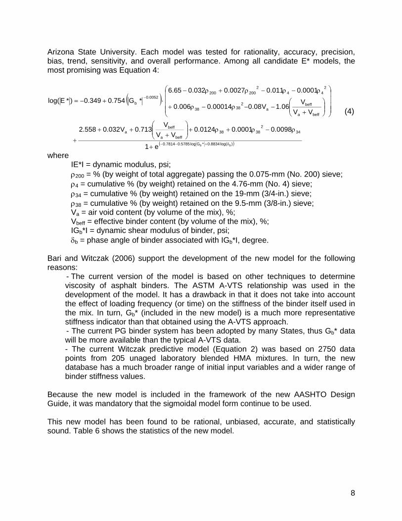
Arizona State University. Each model was tested for rationality, accuracy, precision, bias, trend, sensitivity, and overall performance. Among all candidate E* models, the most promising was Equation 4:
( )
( ))log(8834.0*Glog5785.07814.0
342
3838beffa
beffa
beffa
beffa
23838
244
2200200
0052.0b
bbe1
0098.00001.00124.0VV
V713.0V032.0558.2
VVV
06.1V08.000014.0006.0
0001.0011.00027.0032.065.6*G 754.0349.0)*Elog(
δ+−−
−
+
ρ−ρ+ρ+⎟⎟⎠
⎞⎜⎜⎝
⎛+
++
+
⎟⎟⎟⎟
⎠
⎞
⎜⎜⎜⎜
⎝
⎛
⎟⎟⎠
⎞⎜⎜⎝
⎛+
−−ρ−ρ+
ρ−ρ−ρ+ρ−⋅+−=
(4)
where IE*I = dynamic modulus, psi; ρ200 = % (by weight of total aggregate) passing the 0.075-mm (No. 200) sieve; ρ4 = cumulative % (by weight) retained on the 4.76-mm (No. 4) sieve; ρ34 = cumulative % (by weight) retained on the 19-mm (3/4-in.) sieve; ρ38 = cumulative % (by weight) retained on the 9.5-mm (3/8-in.) sieve; Va = air void content (by volume of the mix), %; Vbeff = effective binder content (by volume of the mix), %; IGb*I = dynamic shear modulus of binder, psi;
δb = phase angle of binder associated with IGb*I, degree. Bari and Witczak (2006) support the development of the new model for the following reasons:
- The current version of the model is based on other techniques to determine viscosity of asphalt binders. The ASTM A-VTS relationship was used in the development of the model. It has a drawback in that it does not take into account the effect of loading frequency (or time) on the stiffness of the binder itself used in the mix. In turn, Gb* (included in the new model) is a much more representative stiffness indicator than that obtained using the A-VTS approach. - The current PG binder system has been adopted by many States, thus Gb* data will be more available than the typical A-VTS data. - The current Witczak predictive model (Equation 2) was based on 2750 data points from 205 unaged laboratory blended HMA mixtures. In turn, the new database has a much broader range of initial input variables and a wider range of binder stiffness values.
Because the new model is included in the framework of the new AASHTO Design Guide, it was mandatory that the sigmoidal model form continue to be used.
This new model has been found to be rational, unbiased, accurate, and statistically sound. Table 6 shows the statistics of the new model.

9
Table 6. Statistics for New Witczak Predictive Model.
Parameter Logarithmic Scale Arithmetic ScaleData points, n 7400 7400
No. of Mixes, Nm 346 346Se 0.21 658 ksiSy 0.66 1459 ksi
Se/Sy 0.32 0.45R2 0.90 0.80
To verify if the new model improves the predictive capability for the full range of the new E* database, Bari and Witczak compared the current Witczak model, the Hirsch model and the new Witczak model. Table 7 shows the comparison of the statistics for the three models. Bari and Witczak concluded that the new Witczak model showed the best predictive strength in comparison with the previous models. This model was developed based on a very large and versatile E* database, while the previous models were based on a much smaller database for a smaller range of mixtures. It must be noted, however, that the comparison against the Hirsch model was not completely “fair”, because an important part of the IGb*I data included in the “new database” are only “estimates” and not direct measurements from lab tests. A more reliable comparison should be done with “measured” data.
Table 7. Comparison of E* Predictive Models [Modified from Bari and Witczak, 2006].
Current Witczak Hirsch New Witczak(Equation 2) (Equation 5-6) (Equation 4)
Total Mix 346 346 346Modified Mix 17 17 17Data Points 7400 7400 7400
Se/Sy 0.60 0.88 0.45R2 0.65 0.23 0.80
Se/Sy 0.35 0.62 0.32R2 0.88 0.61 0.90
ParameterE* Predictive Model
Normal (Arithmetic) Space
Logarithmic Space
3.3 Hirsch Model
The Hirsch model is a rational, though semi-empirical method of predicting asphalt concrete modulus. It is based on an existing version of the law of mixtures, called the Hirsch model, which combines series and parallel elements of the phases. Christensen et al. (2003) presented the application of the Hirsch model to asphalt concrete based on an alternate version of the Hirsch model. Although they evaluated
10
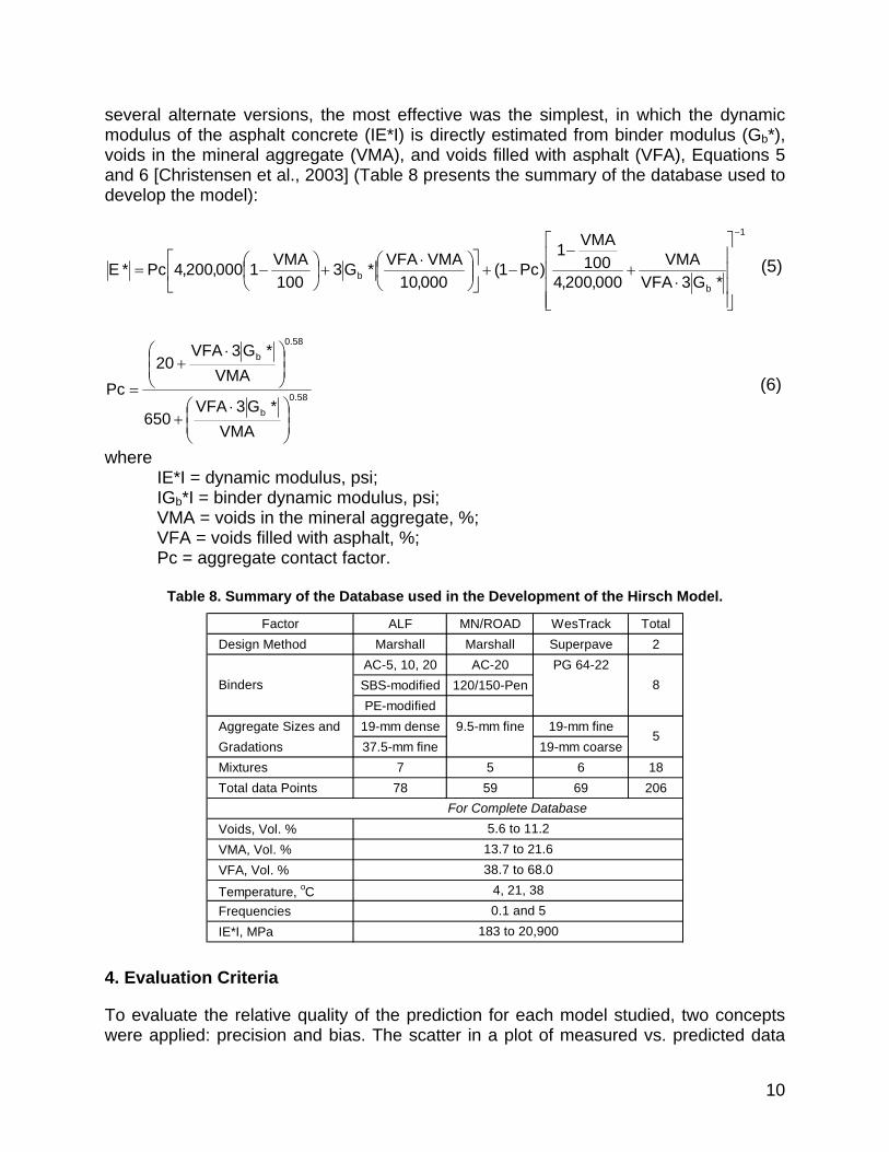
several alternate versions, the most effective was the simplest, in which the dynamic modulus of the asphalt concrete (IE*I) is directly estimated from binder modulus (Gb*), voids in the mineral aggregate (VMA), and voids filled with asphalt (VFA), Equations 5 and 6 [Christensen et al., 2003] (Table 8 presents the summary of the database used to develop the model):
1
bb *G3VFA
VMA000,200,4
100VMA1
)Pc1(000,10VMAVFA*G3
100VMA1000,200,4Pc*E
−
⎥⎥⎥⎥
⎦
⎤
⎢⎢⎢⎢
⎣
⎡
⋅+
−−+⎥
⎦
⎤⎢⎣
⎡⎟⎠⎞
⎜⎝⎛ ⋅
+⎟⎠⎞
⎜⎝⎛ −= (5)
58.0b
58.0b
VMA*G3VFA
650
VMA*G3VFA
20Pc
⎟⎟⎠
⎞⎜⎜⎝
⎛ ⋅+
⎟⎟⎠
⎞⎜⎜⎝
⎛ ⋅+
= (6)
where IE*I = dynamic modulus, psi; IGb*I = binder dynamic modulus, psi; VMA = voids in the mineral aggregate, %; VFA = voids filled with asphalt, %; Pc = aggregate contact factor.
Table 8. Summary of the Database used in the Development of the Hirsch Model.
Factor ALF MN/ROAD WesTrack TotalDesign Method Marshall Marshall Superpave 2
AC-5, 10, 20 AC-20 PG 64-22SBS-modified 120/150-PenPE-modified
Aggregate Sizes and 19-mm dense 9.5-mm fine 19-mm fineGradations 37.5-mm fine 19-mm coarseMixtures 7 5 6 18Total data Points 78 59 69 206
Voids, Vol. %VMA, Vol. %VFA, Vol. %
Temperature, oCFrequenciesIE*I, MPa
4, 21, 380.1 and 5
183 to 20,900
Binders 8
5
For Complete Database5.6 to 11.2
13.7 to 21.638.7 to 68.0
4. Evaluation Criteria
To evaluate the relative quality of the prediction for each model studied, two concepts were applied: precision and bias. The scatter in a plot of measured vs. predicted data

11
represents the precision. Bias, in turn, is the tendency of predicted data to deviate in one direction from the measured data, which corresponds to a systematic error. Performing a linear regression with “zero intercept” in every plot, the slope of the regression line represents the bias. The closer the slope to unity, the less bias. A slope that is less than one indicates a predicted E* is lower than the corresponding measured E* (the model under predicts). A slope that is greater than one indicates a predicted E* is higher than the corresponding measured E* (the model over predicts). The R2 value of the regression represents the precision of the prediction. A high value of R2 indicates a high precision, whereas a low value of R2 represents a low precision. The ideal model would have a precision equal to one (R2=1) and no bias (slope=1). Figures 3a and 3b represent examples of precision and bias. Comparing both figures, the set of data in Figure 3a has low precision (R2=0.856), low bias (1.045) and over-predicts E*. In turn, the set in Figure 3b has high precision (R2=0.955), high bias (0.713) and under predicts E*.
a)
All Mixtures @ 20oC
E*p = 1.045 x E*mR2 = 0.856
1.E+05
1.E+06
1.E+07
1.E+05 1.E+06 1.E+07Measured IE*I, psi
Pred
icte
d IE
*I, p
si
data pointsEqualityLinear w/zero intercept
b)
All Mixtures @ 20oC
E*p = 0.713 x E*mR2 = 0.955
1.E+05
1.E+06
1.E+07
1.E+05 1.E+06 1.E+07Measured IE*I, psi
Pred
icte
d IE
*I, p
si
data pointsEqualityLinear w/zero intercept
Figure 3. Concepts of Precision and Bias.

12
The previous concepts represent a framework to correct predictions of E* in terms of bias. For example, in Figure 3b, the relationship between measured and predicted E* is:
mp *E713.0*E ×= (7) where E*p = predicted dynamic modulus; E*m = measured dynamic modulus. Utilizing Equation 7, a “correction factor” (CF) can be determined to correct the observed bias in E*p:
pcppm *E*ECF*E713.01*E =×=×= (8)
4025.1713.01CF == (9)
where E*p = predicted dynamic modulus; E*m = measured dynamic modulus; E*pc = corrected predicted dynamic modulus; CF = correction factor. The results after applying the CF in the previous example can be seen in Figure 4, in which the “before” (filled diamonds; predicted |E*|) and “after” (empty squares; corrected predicted |E*|) situations are presented. Note that even though the bias was completely eliminated, the precision (R2=0.955) remains the same. This is because the CF is a constant that proportionally shifts every data point along the vertical axis. Therefore, the relative position among them does not change.
All Mixtures @ 20oC
E*p = 0.713 x E*mR2 = 0.955
E*pc = 1.000 x E*mR2 = 0.955
1.E+05
1.E+06
1.E+07
1.E+05 1.E+06 1.E+07Measured IE*I, psi
Pred
icte
d IE
*I, p
si
data pointsCorrectedEqualityLinear w/zero interceptLinear (Corrected)
Figure 4. Example of Correction of Bias.
13
In every stage of this study, a plot of measured vs. predicted E* was developed for every mixture and model evaluated. An additional plot was developed for each model, putting the measured vs. predicted data for all mixtures together (as in Figures 3a, 3b, and 4). In the evaluation of the different predictive models, precision and bias were considered at both the mixture and global level. 5. Mixture MCs and Isochronal Plots
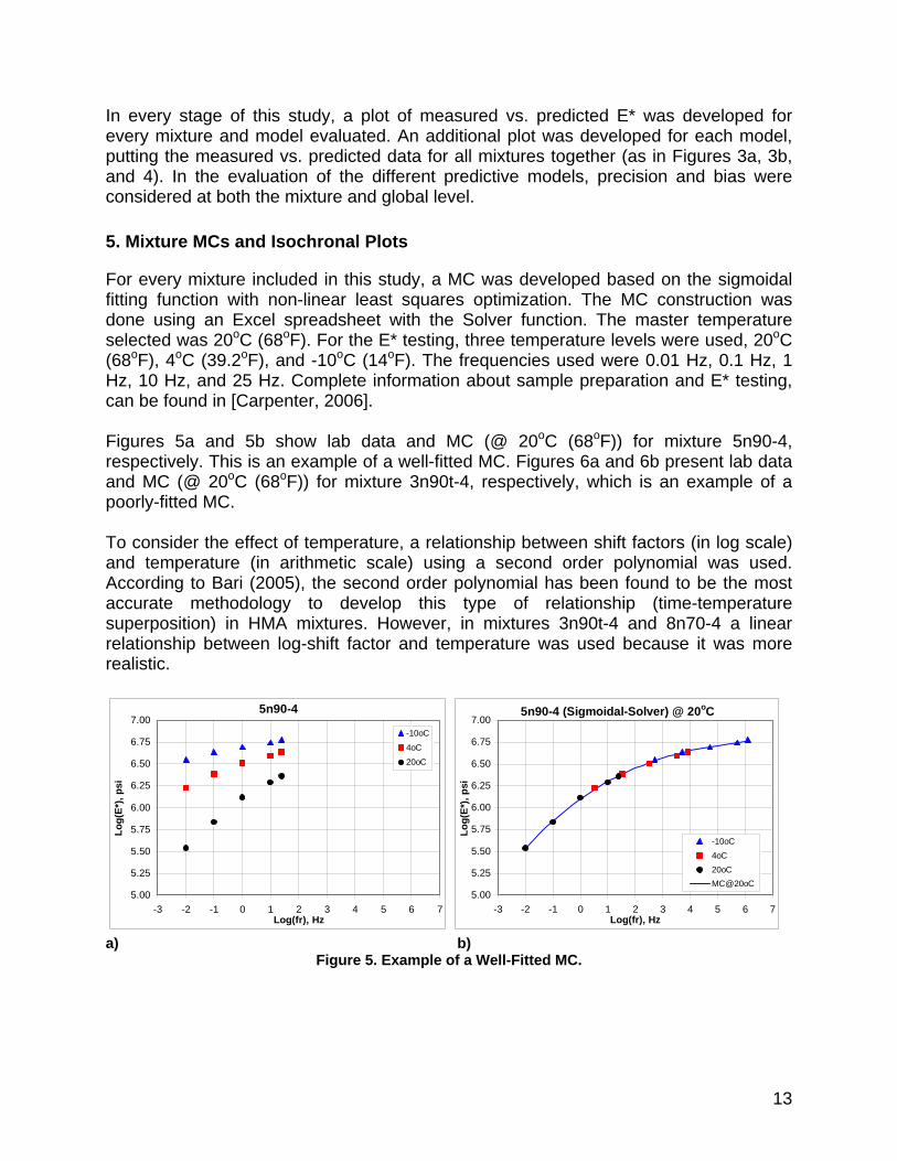
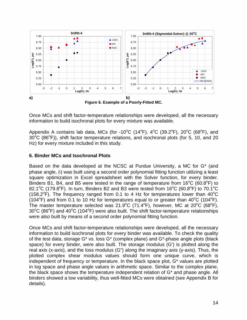
For every mixture included in this study, a MC was developed based on the sigmoidal fitting function with non-linear least squares optimization. The MC construction was done using an Excel spreadsheet with the Solver function. The master temperature selected was 20oC (68oF). For the E* testing, three temperature levels were used, 20oC (68oF), 4oC (39.2oF), and -10oC (14oF). The frequencies used were 0.01 Hz, 0.1 Hz, 1 Hz, 10 Hz, and 25 Hz. Complete information about sample preparation and E* testing, can be found in [Carpenter, 2006]. Figures 5a and 5b show lab data and MC (@ 20oC (68oF)) for mixture 5n90-4, respectively. This is an example of a well-fitted MC. Figures 6a and 6b present lab data and MC (@ 20oC (68oF)) for mixture 3n90t-4, respectively, which is an example of a poorly-fitted MC. To consider the effect of temperature, a relationship between shift factors (in log scale) and temperature (in arithmetic scale) using a second order polynomial was used. According to Bari (2005), the second order polynomial has been found to be the most accurate methodology to develop this type of relationship (time-temperature superposition) in HMA mixtures. However, in mixtures 3n90t-4 and 8n70-4 a linear relationship between log-shift factor and temperature was used because it was more realistic.
5n90-4
5.00
5.25
5.50
5.75
6.00
6.25
6.50
6.75
7.00
-3 -2 -1 0 1 2 3 4 5 6 7Log(fr), Hz
Log(
E*),
psi
-10oC4oC20oC
5n90-4 (Sigmoidal-Solver) @ 20oC
5.00
5.25
5.50
5.75
6.00
6.25
6.50
6.75
7.00
-3 -2 -1 0 1 2 3 4 5 6 7Log(fr), Hz
Log(
E*),
psi
-10oC4oC20oCMC@20oC
a) b)
Figure 5. Example of a Well-Fitted MC.
14
3n90t-4
5.00
5.25
5.50
5.75
6.00
6.25
6.50
6.75
7.00
-3 -2 -1 0 1 2 3 4 5 6 7Log(fr), Hz
Log(
E*),
psi
-10oC
4oC
20oC
3n90t-4 (Sigmoidal-Solver) @ 20oC
5.00
5.25
5.50
5.75
6.00
6.25
6.50
6.75
7.00
-3 -2 -1 0 1 2 3 4 5 6 7Log(fr), Hz
Log(
E*),
psi
-10oC4oC20oCMC@20oC
a) b)
Figure 6. Example of a Poorly-Fitted MC.
Once MCs and shift factor-temperature relationships were developed, all the necessary information to build isochronal plots for every mixture was available. Appendix A contains lab data, MCs (for -10oC (14oF), 4oC (39.2oF), 20oC (68oF), and 30oC (86oF)), shift factor temperature relations, and isochronal plots (for 5, 10, and 20 Hz) for every mixture included in this study. 6. Binder MCs and Isochronal Plots
Based on the data developed at the NCSC at Purdue University, a MC for G* (and phase angle, δ) was built using a second order polynomial fitting function utilizing a least square optimization in Excel spreadsheet with the Solver function, for every binder. Binders B1, B4, and B5 were tested in the range of temperature from 16oC (60.8oF) to 82.1oC (179.8oF). In turn, Binders B2 and B3 were tested from 16oC (60.8oF) to 70.1oC (158.2oF). The frequency ranged from 0.1 to 4 Hz for temperatures lower than 40oC (104oF) and from 0.1 to 10 Hz for temperatures equal to or greater than 40oC (104oF). The master temperature selected was 21.9oC (71.4oF), however, MC at 20oC (68oF), 30oC (86oF) and 40oC (104oF) were also built. The shift factor-temperature relationships were also built by means of a second order polynomial fitting function. Once MCs and shift factor-temperature relationships were developed, all the necessary information to build isochronal plots for every binder was available. To check the quality of the test data, storage G* vs. loss G* (complex plane) and G*-phase angle plots (black space) for every binder, were also built. The storage modulus (G’) is plotted along the real axis (x-axis), and the loss modulus (G”) along the imaginary axis (y-axis). Thus, the plotted complex shear modulus values should form one unique curve, which is independent of frequency or temperature. In the black space plot, G* values are plotted in log space and phase angle values in arithmetic space. Similar to the complex plane, the black space shows the temperature independent relation of G* and phase angle. All binders showed a low variability, thus well-fitted MCs were obtained (see Appendix B for details).
15
7. Results 1st Stage
Table 9 presents the main properties of the mixtures included in this stage.
Table 9. Mixtures Selected 1st Stage.
Max. Agg.PG Sample Size
8n70-4 64-22 B2 13.0 67.6 4.2 19.05n90-4 64-22 B3 13.1 69.5 4 19.03n70-4 64-22 B3 13.2 69.7 4 19.03n90t-4 64-22 B3 13.0 69.3 4 19.03n90-4 76-22 B5 13.6 70.6 4 19.0
5n105-4 76-28 B4 13.2 69.7 4 19.01n80d-4 76-28 B4 14.5 79.3 3 12.5 (SMA)
VFAVMABinderMixture Va
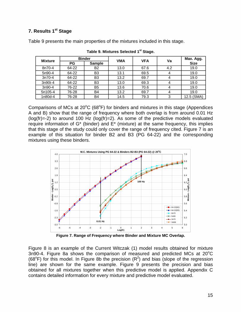
Comparisons of MCs at 20oC (68oF) for binders and mixtures in this stage (Appendices A and B) show that the range of frequency where both overlap is from around 0.01 Hz (log(fr)=-2) to around 100 Hz (log(fr)=2). As some of the predictive models evaluated require information of G* (binder) and E* (mixture) at the same frequency, this implies that this stage of the study could only cover the range of frequency cited. Figure 7 is an example of this situation for binder B2 and B3 (PG 64-22) and the corresponding mixtures using these binders.
M.C. Mixtures Using PG 64-22 & Binders B2-B3 (PG 64-22) @ 20oC
-3.0
-2.3
-1.6
-0.9
-0.2
0.5
1.2
1.9
2.6
3.3
4.0
-6 -5 -4 -3 -2 -1 0 1 2 3 4 5 6Log(fr)
Bin
der -
Log
(Gb*
), ps
i
5.0
5.2
5.4
5.6
5.8
6.0
6.2
6.4
6.6
6.8
7.0
Mix
ture
- Lo
g(E m
*), p
si
64-22(B2)64-22(B3)8n705n903n703n90t0.01 Hz
100 Hz
Figure 7. Range of Frequency where Binder and Mixture MC Overlap.
Figure 8 is an example of the Current Witczak (1) model results obtained for mixture 3n90-4. Figure 8a shows the comparison of measured and predicted MCs at 20oC (68oF) for this model. In Figure 8b the precision (R2) and bias (slope of the regression line) are shown for the same example. Figure 9 presents the precision and bias obtained for all mixtures together when this predictive model is applied. Appendix C contains detailed information for every mixture and predictive model evaluated.

16
a)
Current Witczak (1), 3n90-4 (PG76-22) @ 20oC
4.0
4.5
5.0
5.5
6.0
6.5
7.0
-3 -2 -1 0 1 2 3Log(fr), Hz
Log(
E*),
psi
Measured
Witczak-Estimate
b)
Current Witczak (1), 3n90-4(PG76-22) @ 20oC
E*p = 0.4558 x E*mR2 = 0.9945
1.E+05
1.E+06
1.E+07
1.E+05 1.E+06 1.E+07Measured IE*I, psi
Pred
icte
d IE
*I, p
si
data pointsEqualityLinear w/zero intercept
Figure 8. Results for Mixture 3n90-4 Applying Current Witczak (1) Model.
Current Witczak (1), All Mixtures @ 20oC
E*p = 0.5261 x E*mR2 = 0.7986
1.E+05
1.E+06
1.E+07
1.E+05 1.E+06 1.E+07Mesured IE*I, psi
Pred
icte
d IE
*I, p
si
data pointsEqualityBias
Figure 9. Results for All Mixtures, Applying Current Witczak (1) Model.
Figures 10a and 10b present the summary of the results of precision and bias, respectively, for every mixture and predictive model, as well as grouping all mixtures together (all data). It must be noted at this point, based on Figure 10b, that every result above the line with bias equal to one is over-predicting the E*. Conversely, every result

17
below that line is under predicting E*. Table 10 shows the values obtained for every case.
a)
Precision, Measured E* vs. Predicted E* @ 20oC
0.78
0.80
0.82
0.84
0.86
0.88
0.90
0.92
0.94
0.96
0.98
1.00
1.02
8n70 (64-22[B2])
5n90 (64-22[B3])
3n70 (64-22[B3])
3n90t (64-22[B3])
3n90 (76-22[B5])
5n105 (76-28[B4])
1n80d (76-28[B4])
All Data
Mixtures
R2
C-Witczak (1)C-Witczak (2)C-Witczak (3)N-WitczakHirschOptimum
b)
Bias, Measured E* vs. Predicted E* @ 20oC
0.25
0.50
0.75
1.00
1.25
1.50
1.75
2.00
2.25
2.50
2.75
8n70 (64-22[B2])
5n90 (64-22[B3])
3n70 (64-22[B3])
3n90t (64-22[B3])
3n90 (76-22[B5])
5n105 (76-28[B4])
1n80d (76-28[B4])
All Data
Mixtures
Bia
s
C-Witczak (1)C-Witczak (2)C-Witczak (3)N-WitczakHirschOptimum
Figure 10. Results of Precision and Bias, 1st Stage.

18
Table 10. Results of Precision and Bias, 1st Stage.
PG Sample Bias R2 Bias R2 Bias R2 Bias R2 Bias R2
8n70-4 64-22 B2 9 0.443 0.962 0.447 0.961 0.555 0.922 1.536 0.991 0.634 0.9905n90-4 64-22 B3 9 0.496 0.996 0.481 0.995 0.624 0.999 1.712 0.976 0.686 0.9803n70-4 64-22 B3 9 0.573 0.997 0.556 0.997 0.719 0.983 1.968 0.996 0.794 0.9963n90t-4 64-22 B3 9 0.537 0.998 0.521 0.998 0.675 0.987 1.919 0.994 0.785 0.9943n90-4 76-22 B5 9 0.456 0.994 0.339 0.976 1.523 0.916 0.563 0.943
5n105-4 76-28 B4 9 1.001 0.975 0.700 0.997 2.684 0.988 1.030 0.9931n80d-4 76-28 B4 9 0.676 0.968 0.474 0.995 2.214 0.983 0.768 0.995All Data All Data 63 0.526 0.799 0.463 0.872 1.769 0.899 0.693 0.911C-W (1) Current Witczak: A-VTS from 1-37A default valuesC-W (2) Current Witczak: A-VTS obtained transforming the Binder "G* and δ" data from DSR testC-W (3) Current Witczak: A-VTS from IDOT data base study by UIUC (only for PG 64-22)
N-W New Witczak: [Bari & Witczak, 2006]
Binder C-W (1) C-W (2) HirschMix Data C-W (3) N-W
Based on the previous results, Table 11 shows the rank for each predictive model when they are ordered based on the average precision obtained at mixture level. The coefficient of variation (COV) obtained in each case is very low. Table 12 presents the rank for each predictive model when they are ordered based on the COV of bias obtained at mixture level. In this case, this statistic is more relevant because no matter the level of bias, if a model shows very little variability, it can be corrected by applying a “single” CF valid for all mixtures and practically eliminate the bias in all of them. If a model shows a high variability, to correct the bias, different CFs should be applied. Table 13 presents the rank for precision and bias based on global level results. In this case, there is no average or COV, because every result is a single value, but the result itself is representing a global indicator of the prediction quality for all the typical mixtures studied.
Table 11. Rank of Models Based on Results of Precision at Mixture Level, 1st Stage.
COV8n70-4 5n90-4 3n70-4 3n90t-4 3n90-4 5n105-4 1n80d-4 %
1 C-W (2) 0.961 0.995 0.997 0.998 0.976 0.997 0.995 0.989 0.0144 1.462 Hirsch 0.990 0.980 0.996 0.994 0.943 0.993 0.995 0.985 0.0191 1.943 C-W (1) 0.962 0.996 0.997 0.998 0.994 0.975 0.968 0.984 0.0154 1.574 N-W 0.991 0.976 0.996 0.994 0.916 0.988 0.983 0.978 0.0280 2.875 C-W (3) 0.922 0.999 0.983 0.987 0.973 0.0343 3.52
Rank MixtureModel Average St. Dev.
Table 12. Rank of Models Based on Results of Bias at Mixture Level, 1st Stage. COV
8n70-4 5n90-4 3n70-4 3n90t-4 3n90-4 5n105-4 1n80d-4 %1 Hirsch 0.634 0.686 0.794 0.785 0.563 1.030 0.768 0.751 0.1497 19.922 C-W (3) 0.555 0.624 0.719 0.675 0.643 0.0706 10.983 C-W (1) 0.443 0.496 0.573 0.537 0.456 1.001 0.676 0.597 0.1945 32.554 C-W (2) 0.447 0.481 0.556 0.521 0.339 0.700 0.474 0.503 0.1104 21.965 N-W 1.536 1.712 1.968 1.919 1.523 2.684 2.214 1.937 0.4121 21.28
Rank Mixture Average St. Dev.Model
Table 13. Rank of Models Based on Results of Precision and Bias at Global Level, 1st Stage.
1 Hirsch 0.911 1 Hirsch 0.6932 N-W 0.899 2 C-W (1) 0.5263 C-W (2) 0.872 3 C-W (2) 0.4634 C-W (1) 0.799 4 N-W 1.769Pr
ecis
ion
Bias
All MixesModelRank RankModel All Mixes

19
Using all these criteria, the ideal most promising model would be that one showing the best rank in every category explained. Based on Tables 11, 12, and 13, there is no “ideal” model. It can be clearly seen that the Hirsch model shows the best combined performance compared to any other model. However, it must be noted that the application of the Hirsch model requires knowing the dynamic shear modulus of the binder, at the frequency and temperature desired for mixture dynamic modulus. From a practical point of view, all models showed an acceptable level of precision (R2) at the mixture level. In terms of bias, two groups can be distinguished: the Hirsch, New Witczak, and Current Witczak (2) models with very similar variability of bias, and the Current Witczak (1) model with higher level of variability of bias. The Current Witczak (3) model, although analyzed as a means of reference, was not a candidate in this stage, because it is only applicable for mixtures using PG 64-22 (unmodified binders), which is an important limitation. Based on the results of this stage, the Current Witczak (2), and New Witczak models do not show any significant advantage over the Current Witczak (1) model. Moreover, whereas the Current Witczak (1) model does not need any lab test (it uses the default A and VTS values), an extra effort is needed to obtain the properties of the binder (“G*” and “δ”) to apply the other two models. Although normally it is not a problem to obtain “G*”, “δ” is not so easy to obtain for some modified binders (for instance, see G*-phase angle plot, black space, for binder PG 76-28 in Appendix B. At low “G*” values an important dispersion in the corresponding “δ” values is observed. The same can be concluded comparing both “G*” and “δ” MCs at low frequency values). Consequently, the Hirsch model is selected as the most promising model in this stage. In addition to the Hirsch model, the Current Witczak (1) model should be also included in the second stage of this study, as a means of reference, because it does not need any binder test and it has been considered in previous studies [Garcia, 2007]. 8. Results 2nd Stage
Table 14 presents the main properties of the mixtures studied in this stage.
Table 14. Mixtures Selected 2nd Stage.
Max. Agg.PG Assumed Size
5n70-4 64-22 B2-B3 14.6 72.6 4 9.56n50-4 64-22 B2-B3 13.1 69.4 4 19.09n90-4 64-22 B2-B3 13.2 69.6 4 12.56n50s-4 76-22 B5 16.4 75.7 4 12.5 (SMA)6n90-4 76-22 B5 14.5 72.3 4 9.51n80s-4 76-28 B4 18.4 83.7 3 12.5 (SMA)1n105-4 70-22 B1 13.0 69.2 4 19.02n90-4 70-22 B1 13.1 68.8 4.1 19.0
8n105-4 70-22 B1 14.0 71.5 4 12.5
BinderMixture VMA VaVFA

20
Recall that the properties of the binders used in mixtures evaluated in this stage were unknown. For this reason, based on the PG grade of each mixture’s binder, the properties belonging to samples B1 to B5 were “assumed” to be the same. For the same reasons explained in Section 7 above, this stage of the study covered only the range of frequency from 0.01 to 100 Hz. Figure 11 is an example of the results obtained for mixture 5n70-4 when applying the Hirsch model. Figure 11a shows the comparison of measured and predicted MC at 20oC (68oF) for this model. In Figure 11b the precision (R2) and bias (slope of the regression line) are shown for the same example. Figure 12 presents the precision and bias obtained for all mixtures together when this predictive model is applied. Appendix D contains information in detail for every mixture and predictive model evaluated.
a)
Hirsch, 5n70-4 (PG64-22) @ 20oC
4.0
4.5
5.0
5.5
6.0
6.5
7.0
-3 -2 -1 0 1 2 3Log(fr), Hz
Log(
E*),
psi
Measured
Hirsch-Estimate
b)
Hirsch, 5n70-4 (PG64-22) @ 20oC
E*p = 0.8877 x E*mR2 = 0.9989
1.E+05
1.E+06
1.E+07
1.E+05 1.E+06 1.E+07Measured IE*I, psi
Pred
icte
d IE
*I, p
si
data points
Equality
Linear w/zero intercept
Figure 11. Results for Mixture 5n70-4 Applying Hirsch Model.

21
Hirsch, All Mixtures @ 20oC
E*p = 0.7134 x E*mR2 = 0.9553
1.E+05
1.E+06
1.E+07
1.E+05 1.E+06 1.E+07Measured IE*I, psi
Pred
icte
d IE
*I, p
si
data pointsEqualityLinear (data points)
Figure 12. Results for All Mixtures, Applying Hirsch Model.
Figures 13a and 13b show the results of precision and bias, respectively, for every mixture, as well as grouping all mixtures together (all data). Table 15 presents the values obtained for every case.
a)
Precision, Measured E* vs. Predicted E* @ 20oC
0.84
0.86
0.88
0.90
0.92
0.94
0.96
0.98
1.00
1.02
5n70-4(64-22)
6n50-4(64-22)
9n90-4(64-22)
6n50s-4(76-22)
6n90-4(76-22)
1n80s-4(76-28)
1n105-4(70-22)
2n90-4(70-22)
8n105-4(70-22)
All Data
Mixtures
R2
HirschC-Witczak (1)Optimum
b)
Bias, Measured E* vs. Predicted E* @ 20oC
0.25
0.50
0.75
1.00
1.25
1.50
1.75
2.00
2.25
2.50
2.75
5n70-4(64-22)
6n50-4(64-22)
9n90-4(64-22)
6n50s-4(76-22)
6n90-4(76-22)
1n80s-4(76-28)
1n105-4(70-22)
2n90-4(70-22)
8n105-4(70-22)
All Data
Mixtures
Bia
s
HirschC-Witczak (1)Optimum
Figure 13. Results of Precision and Bias, 2nd Stage.

22
Table 15. Results of Precision and Bias, 2nd Stage.
PG Assum. Bias R2 Bias R2
5n70-4 64-22 B2-B3 9 0.888 0.999 0.578 0.9816n50-4 64-22 B2-B3 9 0.786 0.997 0.565 0.9789n90-4 64-22 B2-B3 9 0.660 0.989 0.440 0.9966n50s-4 76-22 B5 9 0.751 0.987 0.608 0.8806n90-4 76-22 B5 9 0.803 0.989 0.645 0.9841n80s-4 76-28 B4 9 0.764 0.996 0.704 0.9541n105-4 70-22 B1 9 0.626 0.988 0.509 0.9972n90-4 70-22 B1 9 0.656 0.990 0.513 0.997
8n105-4 70-22 B1 9 0.667 0.981 0.561 0.9970.733 0.991 0.569 0.974
0.0866 0.0057 0.0783 0.038111.81 0.57 13.75 3.91
81 0.713 0.955 0.549 0.917C-W (1) Current Witczak: A-VTS from 1-37A default values
All Data
C-W (1)
AverageSt. Dev.COV, %
Mix Binder Data Hirsch
The 2nd stage results show that the Hirsch model has a consistent high precision and low bias for every mixture and also globally, which is in total agreement with the results obtained in the 1st stage (even better). The Current Witczak (1) model, showed a consistent bias, greater than the Hirsch model, but following a similar trend. However, it showed more variability in terms of precision, higher than the 1st stage results. It also showed the lowest precision for a single mixture (6n50s-4). At the global level, the Current Witczak (1) model presented better results than in the 1st stage, but again, clearly worse than the Hirsch model. As in the 1st stage, both models under predict E*. Consequently, the Hirsch model was found appropriate to develop E*-Temperature GCs, which will be presented in the 3rd stage of this study. 9. Results 3rd Stage
To validate the Hirsch model efficacy to develop E*-Temperature GCs, isochronal plots (temperature domain @ 10Hz) of E* lab measurements were compared against isochronal plots, under the same conditions, but applying the Hirsch model. All mixtures used in the 1st and 2nd stages were included in this stage of the study. To consider the effect of mix type, mixtures were grouped as shown in Table 16. For every group of mixtures, a CF, as explained in Section 4, was determined. As presented in Section 1, the design pavement temperatures in Illinois range from 24.4oC (76oF) to 30oC (86oF). Thus, the isochronal plots utilized in this analysis should cover at least this range of interest, but it would be desirable to extend it further than that. In addition, as mentioned in Section 6, the DSR characterization of binders was developed between 16oC (60.8oF) and 82.1oC (179.8oF) for samples B1, B4, and B5, and from 16oC (60.8oF) to 70.1oC (158.2oF) for samples B2 and B3. In the case of the mixtures, the lab characterization was developed in the range of temperatures from -10oC (14oF) to 20oC (68oF). Figure 14 illustrates the situation in which the isochronal plots for samples of PG 64-22 and some of the 19-mm mixtures using these binders have been used as an example, however, the same occurs for every mix and binder

23
utilized. It must be noted that the range of temperatures where binders’ and mixtures’ isochronal plots overlap, is only from 16oC (60.8oF) to 20oC (68oF) which is out of the range of interest. To overcome this problem, the range of temperatures for binders and mixtures was extrapolated. The range of temperatures of binders and mixtures was extrapolated to 10oC (50oF) and 30oC (86oF), respectively. The “overlapping range” (10oC (50oF) to 30oC (86oF)) was used in this part of the study.
Table 16. Groups of Mixtures for 3rd Stage Analysis.
Type, mm Identification PG Sample5n70-4 64-22 B2-B3 (a)6n90-4 76-22 B5 (a)9n90-4 64-22 B2-B3 (a)8n105-4 70-22 B1 (a)8n70-4 64-22 B25n90-4 64-22 B33n70-4 64-22 B33n90t-4 64-22 B36n50-4 64-22 B2-B3 (a)1n105-4 70-22 B1 (a)2n90-4 70-22 B1 (a)3n90-4 76-22 B55n105-4 76-28 B46n50s-4 76-22 B5 (a)1n80d-4 76-28 B41n80s-4 76-28 B4 (a)
(a) : Assumed properties of the equivalent PG binder
19.0
12.5 (SMA)
Mixture Binder
9.5
12.5
Observing the MCs for mixtures and binders in Appendices A and B, it is clear that the binder extrapolation seems to be sound and reliable (low variability and error in the MC fitting process, high level of precision in the shift factor-temperature relationship, wide range of temperatures and frequencies tested, and small range of temperatures in the extrapolation). Nevertheless, the extrapolation of the mixtures was highly influenced by the variability found, especially in the high range of moduli (corresponding to 4oC (39.2oF) and -10oC (14oF)), and the small range of temperatures included in the tests. For this reason, it was not extended further than 30oC (86oF). Moreover, in several cases, the extended temperature range resulted in unreliable predictions and affected the comparison between measured and predicted E* isochronal plots. Figure 15 shows the situation after the extrapolations for the same example showed in Figure 14. It is interesting to observe the isochronal plots for the binders, inside the range of temperatures utilized in this part of the study (10oC (50oF) to 30oC (86oF)). As seen in Figure 16, two clear groups can be differentiated, one including PG 64-22 (both samples), PG 70-22, and PG 76-22 showing higher G* values; and the other, PG 76-28 showing lower G* values. It seems that for these binders and inside this temperature range, the factor affecting the binder G* behavior the most is the low PG grade. Moreover, the differences of G* between both samples of PG 64-22 are, for the majority

24
of the range, more significant than the difference between one of these samples and any other binder, except PG 76-28.
Isochronal Mixtures Using 64-22 & Binders 64-22 @ 10Hz
6.0
6.1
6.2
6.3
6.4
6.5
6.6
6.7
6.8
6.9
7.0
-10 0 10 20 30 40 50 60 70Temperature, oC
Mix
ture
- Lo
g(E*
m),
psi
0.00
0.40
0.80
1.20
1.60
2.00
2.40
2.80
3.20
3.60
4.00
Bin
der -
Log
(G* b
), ps
i
8n705n903n703n90t64-22(B2)64-22(B3)
68oF60.8oF
16
76oF 86oF
Figure 14. Range of Temperatures, Mixtures and Binders Before Extrapolation.
Isochronal Mixtures Using 64-22 & Binders 64-22 @ 10Hz
6.0
6.1
6.2
6.3
6.4
6.5
6.6
6.7
6.8
6.9
7.0
-10 0 10 20 30 40 50 60 70Temperature, oC
Mix
ture
- Lo
g(E*
m),
psi
0.00
0.40
0.80
1.20
1.60
2.00
2.40
2.80
3.20
3.60
4.00
Bin
der -
Log
(G* b
), ps
i
8n705n903n703n90t64-22(B2)64-22(B3)
86oF
50oF
76oF 86oF
Figure 15. Range of Temperatures, Mixtures and Binders After Extrapolation.

25
G* Isochronal All Binders @ 10Hz (Range Studied)
2.0
2.2
2.4
2.6
2.8
3.0
3.2
3.4
3.6
3.8
4.0
4.2
10 15 20 25 30Temperature, oC
Log(
G*)
, psi
70-22(B1)64-22(B2)64-22(B3)76-28(B4)76-22(B5)
Range of Interest76oF 86oF
24.4
Figure 16. Effect of Binder Inside the Range Studied.
Figures 17a to 17d show isochronal plots at 10 Hz for the four groups of mixtures presented in Table 16. For every group, a “characteristic equation” was determined fitting a second order polynomial (shown in each plot) with the purpose to “represent” the set of curves in each group and simplify later comparisons. The group of 19.0-mm mixtures represents a special case, because the use of binder PG 76-28 in mixture 5n105 affects that mixture in such a way that it was treated separately. That is the reason why for the two equations in Figure 17c. The equation at the bottom of the plot represents the characteristic equation for mixture 5n105 and the equation at the top right, all other 19.0-mm mixtures, except mixtures 3n90 and 3n90t. These two mixtures were disregarded at this step, because they showed a significant variability in the lab data and do not follow the same trend as the other mixtures. It is surmised that the E* lab test was the cause. Similarly, mixture 6n50, in the group of 12.5-mm SMA mixtures, was not considered in the following analysis. Observing Figures 17a to 17d, it can be noted that at temperatures higher than around 20oC (68oF) the curves tend to separate. This effect is thought to be a consequence of the extrapolation of the mixtures lab data to 30oC (86oF), as explained earlier. It is interesting to note in Figure 17c that it is not possible to find a trend among the mixtures using PG 64-22 and PG 70-22, based on the PG type (VMA, VFA, and Va are very similar). This is in agreement with what was explained in Figure 16. It seems that the variability of the E* lab test is masking the effect of the behavior of PG 64-22 and PG 70-22 inside this range of temperatures (10oC (50oF) and 30oC (86oF)).

26
Isochronal E*, 9.5mm Mixtures @ 10Hz (Lab Data)
y = -0.0004x2 - 0.0114x + 6.5762R2 = 0.9609
5.7
5.8
5.9
6.0
6.1
6.2
6.3
6.4
6.5
6.6
6.7
6.8
6.9
-10 -5 0 5 10 15 20 25 30Temperature, oC
log(
E*),
psi
5n70(64-22)6n90(76-22)Char.Eq.
Isochronal E*, 12.5mm Mixtures @ 10Hz (Lab Data)
y = -0.0002x2 - 0.0115x + 6.6381R2 = 0.9941
5.7
5.8
5.9
6.0
6.1
6.2
6.3
6.4
6.5
6.6
6.7
6.8
6.9
-10 -5 0 5 10 15 20 25 30Temperature, oC
log(
E*),
psi
9n90(64-22)
8n105(70-22)
Char.Eq.
a) b)
Isochronal E*, 19.0mm Mixtures @ 10Hz (Lab Data)
y = -0.0004x2 - 0.0103x + 6.6532R2 = 0.9728
y = -0.0003x2 - 0.0164x + 6.4332R2 = 0.9984
5.7
5.8
5.9
6.0
6.1
6.2
6.3
6.4
6.5
6.6
6.7
6.8
6.9
-10 -5 0 5 10 15 20 25 30Temperature, oC
log(
E*),
psi
8n70(64-22)5n90(64-22)3n70(64-22)6n50(64-22)1n105(70-22)2n90(70-22)3n90t(64-22)3n90(76-22)5n105(76-28)Char.Eq.Char.Eq.(76-28)
Isochronal E*, 12.5mm-SMA Mixtures @ 10Hz (Lab Data)
y = -0.0003x2 - 0.0140x + 6.4798R2 = 0.9581
5.7
5.8
5.9
6.0
6.1
6.2
6.3
6.4
6.5
6.6
6.7
6.8
6.9
-10 -5 0 5 10 15 20 25 30Temperature, oC
log(
E*),
psi
6n50s(76-22)
1n80s(76-28)
1n80d(76-28)
Char.Eq.
c) d)
Figure 17. Isochronal Plots from Lab Data for Every Group of Mixtures (@ 10 Hz).
27
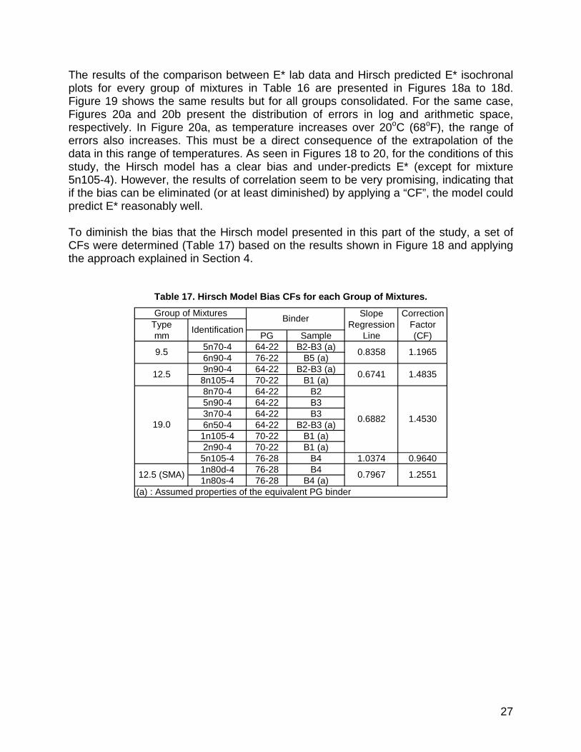
The results of the comparison between E* lab data and Hirsch predicted E* isochronal plots for every group of mixtures in Table 16 are presented in Figures 18a to 18d. Figure 19 shows the same results but for all groups consolidated. For the same case, Figures 20a and 20b present the distribution of errors in log and arithmetic space, respectively. In Figure 20a, as temperature increases over 20oC (68oF), the range of errors also increases. This must be a direct consequence of the extrapolation of the data in this range of temperatures. As seen in Figures 18 to 20, for the conditions of this study, the Hirsch model has a clear bias and under-predicts E* (except for mixture 5n105-4). However, the results of correlation seem to be very promising, indicating that if the bias can be eliminated (or at least diminished) by applying a “CF”, the model could predict E* reasonably well. To diminish the bias that the Hirsch model presented in this part of the study, a set of CFs were determined (Table 17) based on the results shown in Figure 18 and applying the approach explained in Section 4.
Table 17. Hirsch Model Bias CFs for each Group of Mixtures.
Slope CorrectionType Regression Factormm PG Sample Line (CF)
5n70-4 64-22 B2-B3 (a)6n90-4 76-22 B5 (a)9n90-4 64-22 B2-B3 (a)
8n105-4 70-22 B1 (a)8n70-4 64-22 B25n90-4 64-22 B33n70-4 64-22 B36n50-4 64-22 B2-B3 (a)
1n105-4 70-22 B1 (a)2n90-4 70-22 B1 (a)
5n105-4 76-28 B4 1.0374 0.96401n80d-4 76-28 B41n80s-4 76-28 B4 (a)
(a) : Assumed properties of the equivalent PG binder
0.7967
Group of Mixtures BinderIdentification
0.8358
0.6741
1.1965
1.4835
12.5 (SMA) 1.2551
1.453019.0
9.5
12.5
0.6882

28
a)
9.5mm(64-22, 76-22) Mixtures @ 10Hz
y = 0.8358xR2 = 0.9324
1.E+05
1.E+06
1.E+07
1.E+05 1.E+06 1.E+07Measured IE*I, psi
Pred
icte
d IE
*I, p
si
5n706n90Equality
b)
12.5mm(64-22, 70-22) Mixtures @ 10Hz
y = 0.6741xR2 = 0.9701
1.E+05
1.E+06
1.E+07
1.E+05 1.E+06 1.E+07Measured IE*I, psi
Pred
icte
d IE
*I, p
si
9n90
8n105
Equality
c)
19.0mm(64-22, 70-22) Mixtures @ 10Hz
y = 0.6882xR2 = 0.9397
1.E+05
1.E+06
1.E+07
1.E+05 1.E+06 1.E+07Measured IE*I, psi
Pred
icte
d IE
*I, p
si
8n705n903n706n501n1052n90Equality
d)
19.0mm(76-28) Mixtures @ 10Hz
y = 1.0374xR2 = 0.9862
1.E+05
1.E+06
1.E+07
1.E+05 1.E+06 1.E+07Measured IE*I, psi
Pred
icte
d IE
*I, p
si
5n105Equality
Figure 18. Results for Every Group of Mixtures.

29
All Mixtures @ 10Hz
y = 0.7214xR2 = 0.8769
1.E+05
1.E+06
1.E+07
1.E+05 1.E+06 1.E+07Measured IE*I, psi
Pred
icte
d IE
*I, p
si
9.5mm12.5mm19.0mm12.5mm(SMA)Equality
Figure 19. Results for All Groups of Mixtures Consolidated.
a)
Distribution of Error, All Mixtures @ 10Hz
-0.4
-0.3
-0.2
-0.1
0.0
0.1
0.2
0.3
0.4
5 10 15 20 25 30 35Temperature, oC
log(
E*m) -
log(
E*p)
, ksi
9.5mm12.5mm19.0mm12.5mm(SMA)Equality
b)
Distribution of Error, All Mixtures @ 10Hz
-900-800-700-600-500-400-300-200-100
0100200300400500600700800900
1,0001,1001,2001,300
5 10 15 20 25 30 35Temperature, oC
E*m -
E*p,
ksi
9.5mm12.5mm19.0mm12.5mm(SMA)Equality
Figure 20. Distribution of Errors, All Groups of Mixtures Consolidated.

30
The results obtained after applying the CFs (Table 17) to every Hirsch E* prediction for every mixture can be seen in Figures 21a to 21d. To provide a representative reference of comparison, the “characteristic equations” of lab isochronal plots (Figure 17) corresponding to each group of mixtures are also shown. Figure 22 presents the same results but for all groups consolidated. For the same case, Figures 23a and 23b show the distribution of errors in log and arithmetic space, respectively. Observe in Figure 22, that not only the bias was eliminated after the correction (from 0.7214 to 1.0), but also the correlation coefficient was increased at global level (from 0.8769 to 0.9543). At the mixture level (although not shown), obviously, the bias for each group was eliminated but the correlation coefficients remained the same for each group. A comparison of Figures 20a and 23a indicates that the range of errors decreased in the range of temperatures from 10oC (50oF) to 20oC (68oF), a little at 25oC (77oF) and remained almost the same at 30oC (86oF). After the correction there is no bias and the errors are well distributed around the zero-error line. Note in Figure 23b, that even though the after-correction situation is clearly better than the previous one (much higher R2 and no bias), the arithmetic error in some cases could reach values around +/- 350 ksi. This should be considered when using this kind of prediction for pavement design purposes. However, there is an intrinsic variability in the E* test in the lab itself, that can not be taken into account by the predictive model. In other words, it seems that the predictive model (Hirsch model in this case) is potentially nearly as accurate as measured modulus values and for practical applications, using E* predicted by the Hirsch model is probably as effective as using measured E* values [Christensen et al., 2003]. Based on the previous results, it seems that the Hirsch model, after applying the CFs to eliminate the bias, is appropriate to develop “E*-Temperature GCs.”

31
a)
E* Isochronal, 9.5mm Mixtures @ 10Hz (Hirsch-Corrected)
5.7
5.8
5.9
6.0
6.1
6.2
6.3
6.4
6.5
6.6
6.7
6.8
6.9
10 12 14 16 18 20 22 24 26 28 30Temperature, oC
log(
E*),
psi
5n70(64-22)6n90(76-22)Char.Eq.
b)
E* Isochronal, 12.5 mm Mixtures @ 10Hz (Hirsch-Corrected)
5.7
5.8
5.9
6.0
6.1
6.2
6.3
6.4
6.5
6.6
6.7
6.8
6.9
10 12 14 16 18 20 22 24 26 28 30Temperature, oC
log(
E*),
psi
9n90(64-22)
8n105(70-22)
Char.Eq.
c)
E* Isochronal, 19.0mm Mixtures @ 10Hz (Hirsch-Corrected)
5.7
5.8
5.9
6.0
6.1
6.2
6.3
6.4
6.5
6.6
6.7
6.8
6.9
10 12 14 16 18 20 22 24 26 28 30Temperature, oC
log(
E*),
psi
8n70(64-22)5n90(64-22)3n70(64-22)6n50(64-22)1n105(70-22)2n90(70-22)5n105(76-28)Char.Eq.Char.Eq.(76-28)
d)
E* Isochronal, 12.5mm-SMA Mixtures @ 10Hz (Hirsch-Corrected)
5.7
5.8
5.9
6.0
6.1
6.2
6.3
6.4
6.5
6.6
6.7
6.8
6.9
10 12 14 16 18 20 22 24 26 28 30Temperature, oC
log(
E*),
psi
1n80s(76-28)
1n80d(76-28)
Char.Eq.
Figure 21. Isochronal Plots for Group of Mixtures After Applying CF to Hirsch E* Predictions.
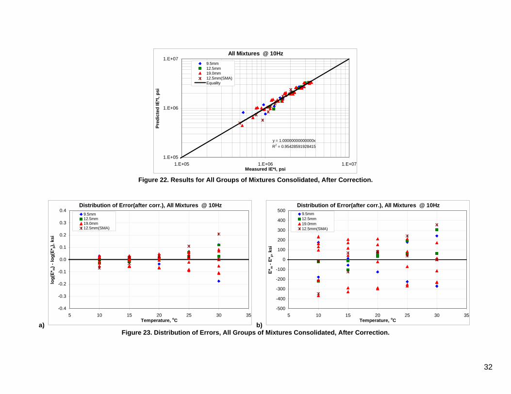
32
All Mixtures @ 10Hz
y = 1.00000000000000xR2 = 0.95428591928415
1.E+05
1.E+06
1.E+07
1.E+05 1.E+06 1.E+07Measured IE*I, psi
Pred
icte
d IE
*I, p
si
9.5mm12.5mm19.0mm12.5mm(SMA)Equality
Figure 22. Results for All Groups of Mixtures Consolidated, After Correction.
a)
Distribution of Error(after corr.), All Mixtures @ 10Hz
-0.4
-0.3
-0.2
-0.1
0.0
0.1
0.2
0.3
0.4
5 10 15 20 25 30 35Temperature, oC
log(
E*m) -
log(
E*p)
, ksi
9.5mm12.5mm19.0mm12.5mm(SMA)
b)
Distribution of Error(after corr.), All Mixtures @ 10Hz
-500
-400
-300
-200
-100
0
100
200
300
400
500
5 10 15 20 25 30 35Temperature, oC
E*m -
E*p,
ksi
9.5mm12.5mm19.0mm12.5mm(SMA)
Figure 23. Distribution of Errors, All Groups of Mixtures Consolidated, After Correction.

33
10. E*-Temperature GCs
For representative HMAs and binders included in this study, the Hirsch model (corrected to eliminate the bias for every mixture group in Table 17) was utilized to develop E*-Temperature GCs that represent the typical conditions and materials for pavement design purposes in the range of temperatures from 10oC (50oF) to 30oC (86oF). The Hirsch model (Equations 5 and 6) needs G*, VMA, VFA, and Va as input parameters. In the case of the binder, the properties studied at the NCSC were used as generic. This means that for PG 64-22, the average G* values from samples B2 and B3 were assumed as representative; for PG 70-22, those from sample B1; for PG 76-22, those corresponding to sample B5; and for PG 76-28, the G* values from sample B4. Volumetric property values considered typical by IDOT were utilized. Table 18 shows a summary of the “generic” properties.
Table 18. Generic Properties for each Group of Mixtures.
Mixture Group Binder VMA VFA Vamm PG
64-22 14.7 72.8 476-22 14.7 72.8 464-22 14.0 71.4 470-22 14.0 71.4 464-22 13.0 69.2 470-22 13.0 69.2 476-28 13.0 69.2 4
12.5 (SMA) 76-28 16.5 75.8 4
9.5
12.5
19.0
Figures 24 to 27 present the E*-Temperature GCs for every group of mixtures and binder type. In every Figure, the curves contained in the current IDOT Full- Depth HMA pavement design procedure (shown in Figure 1) are also included as a means of comparison. Even though the GCs were developed using the Hirsch model, a set of “practical equations” (shown in Table 19) were also obtained, fitting a second order polynomial equation to every Hirsch-model GC. As seen in Table 19, R2 in each case is practically equal to one, therefore, for any practical purpose when an equation is needed instead of a plot, they can be utilized. Comparing Figures 25 and 26, it is clear that the GCs for 12.5-mm and 19.0-mm mixtures (PG 64-22 and PG 70-22) are, for all practical purposes, the same. Table 20 shows the comparison (the E* differences range from 2 ksi (at 10oC (50oF)) to 13 ksi (at 21.1oC (70oF) and 23.9oC (75oF)). This, although not expected, can be explained due to the fact that there are two opposite effects interacting together; 19.0-mm mixtures have lower “generic” VMA and VFA, but the same “generic” Va than 12.5-mm mixtures (Table 18). This implies that the first “generic” group should obtain higher E* values than the second one (all other conditions the same). However, at the same time, the CF applied to 19.0-mm mixtures is lower than that of the 12.5-mm group (Table 17), compensating the opposite effect of the volumetric properties.

34
E*-Temperature Generic Curve, 9.5mm Mixtures @ 10Hz
50 55 60 65 70 75 80 85 90 95HMA Temperature, oF
HM
A E
*, ks
i
64-2276-22AC-20AC-10
200
300
400
500
600
1000
700800900
2000
3000
4000
Figure 24. GCs for 9.5-mm Mixtures @ 10Hz.
E*-Temperature Generic Curve, 12.5mm Mixtures @ 10Hz
50 55 60 65 70 75 80 85 90 95HMA Temperature, oF
HM
A E
*, ks
i
64-2270-22AC-20AC-10
200
300
400
500
600
1000
700800900
2000
3000
4000
Figure 25. GCs for 12.5-mm Mixtures @ 10Hz.

35
E*-Temperature Generic Curve, 19.0mm Mixtures @ 10Hz
50 55 60 65 70 75 80 85 90 95HMA Temperature, oF
HM
A E
*, ks
i
64-2270-2276-28AC-20AC-10
200
300
400
500
600
1000
700800900
2000
3000
4000
Figure 26. GCs for 19.0-mm Mixtures @ 10Hz.
E*-Temperature Generic Curve, 12.5mm-SMA Mixtures @ 10Hz
50 55 60 65 70 75 80 85 90 95HMA Temperature, oF
HM
A E
*, ks
i
76-28AC-20AC-10
200
300
400
500
600
1000
700800900
2000
3000
4000
Figure 27. GCs for 12.5-mm-SMA Mixture @ 10Hz.

36
Table 19. Polynomial Representation of GCs @10Hz, for each Group of Mixtures.
Mixture Group Bindermm PG a b c
9.5mm 64-22 -1.3205052E-04 0.0039480 3.5495836 0.999976-22 -8.9400182E-05 -0.0032276 3.8190386 0.9998
12.5mm 64-22 -1.3266364E-04 0.0041143 3.6427166 0.999970-22 -9.7164697E-05 -0.0014198 3.8266452 0.9999
19.0mm 64-22 -1.3353436E-04 0.0043540 3.6331791 0.999970-22 -9.8370278E-05 -0.0011330 3.8156863 0.999976-28 -4.2616090E-05 -0.0113789 3.9434108 0.9998
12.5mm-SMA 76-28 -3.6499939E-05 -0.0125928 4.0669332 0.9998 log(E*) = a x T2 + b x T + c (E*, ksi; T, oF)
R2Polynomial Coefficients
Table 20. Comparison of E* for 12.5-mm vs. 19.0-mm Mixtures.
TemperatureoF 12.5mm 19.0mm 12.5mm 19.0mm50 3,287 3,289 3,256 3,25955 2,936 2,942 2,849 2,85660 2,582 2,592 2,464 2,47565 2,237 2,249 2,108 2,12070 1,908 1,922 1,783 1,79675 1,603 1,617 1,491 1,50480 1,327 1,339 1,234 1,24685 1,081 1,093 1,009 1,02090 868 878 816 82695 686 694 653 661
E*, ksiPG 64-22 PG 70-22
From a practical pavement design point of view, it is reasonable to consolidate the 12.5- and 19.0-mm mixtures in only one group, “12.5-mm & 19.0-mm” mixtures. In practical terms, the new group “12.5-mm & 19.0-mm” mixtures is represented by the same GCs presented in Table 19 as 12.5-mm mixtures for PG 64-22 and PG 70-22 (because they are on the conservative side). Table 20 is also useful to quantify the effect of binder for the properties of the mixtures and range of temperatures considered. Comparing PG 64-22 and PG 70-22 for 12.5-mm and 19.0-mm mixture groups, it can be seen that the E* differences range from 30 ksi (at 10oC (50oF)) to 129 ksi (at 18.3oC (65oF)). These differences, although not very significant, are around ten times those found between both mixtures when using the same binder type. Similarly, when comparing the effect of PG 64-22 and PG 76-22 on E* for 9.5-mm mixtures, the differences range from -81.4 ksi (at 23.9oC (75oF), E* for PG 64-22 higher than E* for PG 76-22) to 106 ksi (at 10oC (50oF), E* for PG 76-22 higher than E* for PG 64-22). The effect of binder type was previously mentioned in Section 9, when comparing isochronal plots for every binder in the range of interest for this study. The results suggest that the impact of these binders is not significant in the resulting E* values under the conditions studied. However, since only one sample was available for every binder type studied (except for PG 64-22 with two samples) it is not

37
possible to know the variability of G* of each binder type. Therefore, it is not appropriate with the information available at this time, to consolidate binders PG 64-22, PG 70-22, and PG 76-22 in only one group. Consequently, Table 21 and Figures 28 to 31 present the final GCs proposed in this study.
Table 21. E*-Temperature GCs @ 10Hz Proposed in this Study.
Mixture Group Binder Equationmm PG No a b c
9.5mm 64-22 1 -1.3205052E-04 0.0039480 3.549583676-22 2 -8.9400182E-05 -0.0032276 3.8190386
12.5mm & 19.0mm 64-22 3 -1.3266364E-04 0.0041143 3.642716670-22 4 -9.7164697E-05 -0.0014198 3.8266452
19.0mm 76-28 5 -4.2616090E-05 -0.0113789 3.943410812.5mm-SMA 76-28 6 -3.6499939E-05 -0.0125928 4.0669332
log(E*) = a x T2 + b x T + c (E*, ksi; T, oF)
Polynomial Coefficients
E*-Temperature Generic Curve, 9.5mm Mixtures @ 10Hz
50 55 60 65 70 75 80 85 90 95HMA Temperature, oF
HM
A E
*, ks
i
64-22
76-22
200
300
400
500
600
1000
700800900
2000
3000
4000
Figure 28. GCs Proposed for 9.5-mm Mixtures @ 10Hz.
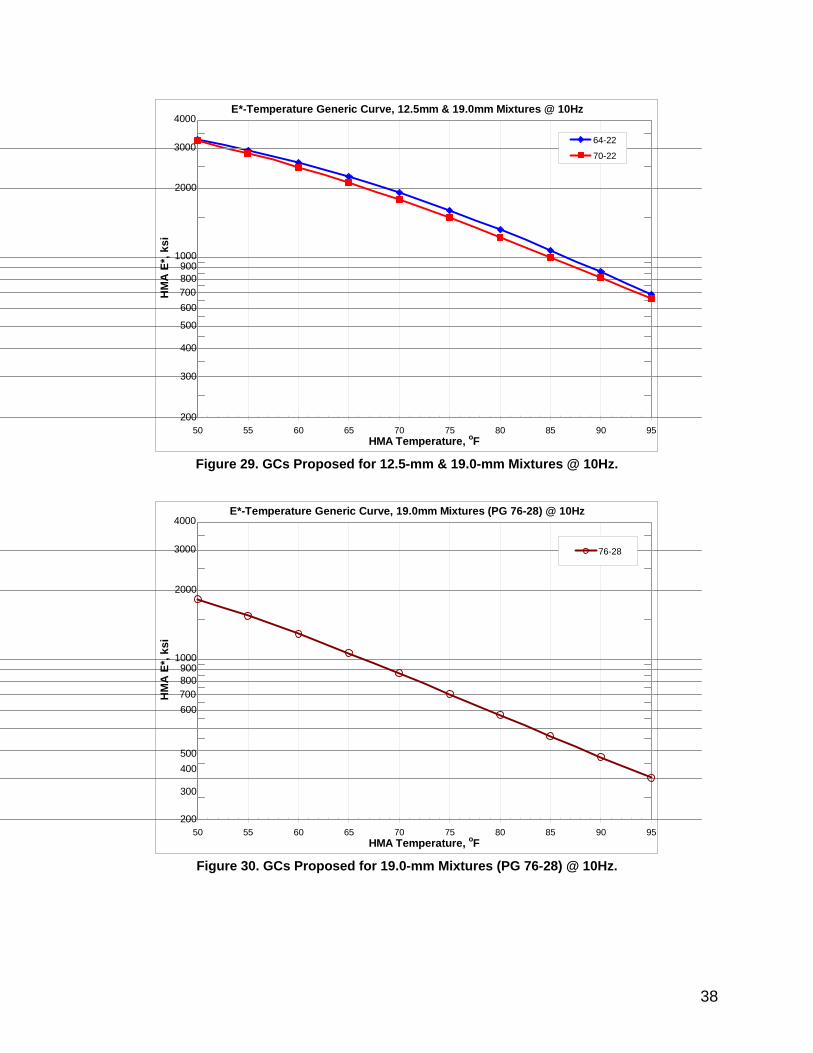
38
E*-Temperature Generic Curve, 12.5mm & 19.0mm Mixtures @ 10Hz
50 55 60 65 70 75 80 85 90 95HMA Temperature, oF
HM
A E
*, ks
i
64-22
70-22
200
300
400
500
600
1000
700800900
2000
3000
4000
Figure 29. GCs Proposed for 12.5-mm & 19.0-mm Mixtures @ 10Hz.
E*-Temperature Generic Curve, 19.0mm Mixtures (PG 76-28) @ 10Hz
50 55 60 65 70 75 80 85 90 95HMA Temperature, oF
HM
A E
*, ks
i
76-28
200
300
400500
600
1000
700800900
2000
3000
4000
Figure 30. GCs Proposed for 19.0-mm Mixtures (PG 76-28) @ 10Hz.

39
E*-Temperature Generic Curve, 12.5mm-SMA Mixtures @ 10Hz
50 55 60 65 70 75 80 85 90 95HMA Temperature, oF
HM
A E
*, ks
i76-28
200
300
400
500
600
1000
700800900
2000
3000
4000
Figure 31. GCs Proposed for 12.5-mm-SMA Mixtures @ 10Hz.
11. Application of Proposed GCs
To verify the applicability of the proposed GCs, the five mixtures utilized in the ELHMAP project at ATREL (Table 22) were compared against the corresponding GC (Table 21). Appendix E contains lab data, MCs (for -10oC (14oF), 4oC (39.2oF), 20oC (68oF), and 30oC (86oF)), shift factor-temperature relations, and isochronal plots (for 5, 10, and 20 Hz) for every mixture from ATREL. Figures 32 to 34 show the comparisons and Table 23 summarizes the differences between the lab data and the GCs at different temperatures.
Table 22. Mixtures Utilized in ELHMAP Project at ATREL.
Binder VaName Type, mm PG %1111 19.0 SBS 70-22 4.01112 19.0 64-22 4.01113 12.5 SBS 70-22 4.01114* 19.0 64-22 2.53809 12.5-SMA SBS 76-28 4.0
* : This is a Rich Bottom Mixture
Mixture

40
12.5&19.0mm Mixtures, PG 64-22 @ 10Hz
50 55 60 65 70 75 80 85 90 95HMA Temperature, oF
HM
A E
*, ks
i
11121114Generic (64-22)
200
300
400
500
600
1000
700800900
2000
3000
4000
Figure 32. GC 12.5-mm&19.0-mm (PG 64-22) Mixtures vs. Lab Data Curves, Mixtures 1112 and 1114
@ 10Hz.
12.5&19.0mm Mixtures, PG 70-22 @ 10Hz
50 55 60 65 70 75 80 85 90 95HMA Temperature, oF
HM
A E
*, ks
i
11111113Generic (70-22)
200
300
400
500
600
1000
700800900
2000
3000
4000
Figure 33. GC 12.5-mm&19.0-mm (PG 70-22) Mixtures vs. Lab Data Curves, Mixtures 1111 and 1113
@ 10Hz.

41
12.5mm-SMA Mixtures, PG 76-28 @ 10Hz
50 55 60 65 70 75 80 85 90 95HMA Temperature, oF
HM
A E
*, ks
i
3809Generic(76-28)
200
300
400
500
600
1000
700800900
2000
3000
4000
Figure 34. GC 12.5-mm-SMA (PG 76-28) Mixtures vs. Lab Data Curves for Mixture 3809 @ 10Hz.
Table 23. E* from ATREL Mixtures MCs vs. E* from Corresponding GC.
TemperatureoF 1111 1112 1113 1114 380950 24 -278 375 -49 -65859 -229 -265 124 -135 -91268 -227 -182 -14 -70 -93477 -39 -85 -56 90 -81186 159 -29 -36 226 -632
MixtureE* Difference Respect to Generic Curve, ksi
Figures 32 to 34 and Table 23 (for every ATREL mixture except SMA 3809), indicate the E* difference with respect to the corresponding GC is in complete agreement with the range of error found previously (around +/- 350 ksi, Figure 23b). Note that the volumetric properties of ATREL mixtures were unknown, except Va (Table 22). Va for mixtures 1111, 1112, and 1113 are in agreement with the generic properties used to develop the GCs (Table 18). Mixture 1114 uses different Va than the GC; however, it is thought that this difference is not significant. Although this application can not be taken as a validation of the proposed GCs, because of the few mixtures utilized, the results seem very promising, except for SMA mixtures. The SMA GC was developed based on only two lab mixtures and more test data are needed. Note that SMA mixtures were not included in the data base used to develop the Hirsch model [Christensen et al., 2003].

42
12. Summary and Conclusions
The most important Hot Mix Asphalt (HMA) property influencing the structural response of a flexible pavement is the HMA modulus (EHMA). Temperature and frequency of loading (or its inverse, load pulse duration) significantly influence EHMA. A three-stage study to evaluate HMA dynamic modulus predictive models using typical IDOT mixtures and binders was conducted with the objective to propose HMA modulus-temperature generic relations for pavement design applications. Based on other studies and information, the frequency of interest has been identified as 10 Hz. The range of design pavement HMA temperature (24.4oC (76oF) to 30oC (86oF)), contained in Illinois’ current full-depth HMA design procedure was the range of interest in this study. Three E* predictive models were evaluated: the current Witczak model (using different ways to obtain A-VTS input parameters), the new Witczak model, and the Hirsch model. The most promising model, for the mixtures and binders studied, was the Hirsch model. This model showed the highest precision and the lowest bias of all the models. The Hirsch model provided good performance even when the G* of the binder was “assumed” (based on other typical binders of the same PG), instead of being measured directly in the lab. For every mixture studied, the Hirsch model “under predicted” the E* (with the exception of a 19.0-mm mixture using PG 76-28). Based on the bias found for each group of mixtures when applying the Hirsch model, a set of “CFs” was determined. After applying the CFs to each group of mixtures, the E* predicted with the Hirsch model showed no appreciable bias. The binder and mixture isochronal plots in the temperature range of interest (24.4oC (76oF) to 30oC (86oF)), suggest that for the binders and mixtures studied, there is not a significant impact (difference) in the resulting E* using PG 64-22, PG 70-22 or PG 76-22 (all other properties being the same). However, there is a significant impact (difference) when using PG 76-28. The five binder samples utilized in this study were insufficient to make a decision to consolidate the groups using PG 64-22, PG 70-22, and PG 76-22; therefore, they were not consolidated. Based on some generic volumetric property (VMA, VFA, Va) information provided by IDOT for typical Illinois mixtures and binder G* relations for five Illinois binders tested at the NCSC, a set of “E*-Temperature GCs” were developed for five different groups of mixtures, applying the Hirsch model (between 10oC (50oF) and 30oC (86oF) at 10 Hz). The GCs for each group of mixtures were compared with the E*-Temperature relations used in the current IDOT full-depth HMA pavement design procedure. In general, the GCs predict much higher HMA E* values for a given temperature and mixture than the current IDOT curves, except when PG 76-28 is used in a 19.0-mm mixture.

43
However, comparing the resulting GCs for 12.5-mm and 19.0-mm mixture groups, it was found that both can be considered equal for pavement design. Accordingly, both groups were consolidated into one group. As a result, a set of six GCs (by means of second order polynomial equations and plots) were presented as the final “proposed GCs”: 1) 9.5-mm mixtures using PG 64-22, 2) 9.5-mm mixtures using PG 70-22, 3) 12.5-mm and 19.0-mm mixtures using PG 64-22, 4) 12.5-mm and 19.0-mm mixtures using PG 70-22, 5) 19.0-mm mixtures using PG 76-28, and 6) 12.5-mm SMA mixtures using PG 76-28. To verify the applicability of the proposed GCs, five mixtures utilized in the ELHMAP project at ATREL were compared against the corresponding GC in the range of 10oC (50oF) to 30oC (86oF) at 10 Hz. The results of this comparison were favorable for 12.5-mm and 19.0-mm mixtures using PG 64-22 and PG 70-22. The result for 12.5-mm SMA using PG 76-28 was “out of range.” There is an intrinsic variability in the E* test in the lab itself, that can not be taken into account by a predictive model. In the words of the authors of the Hirsch model: “…Modulus predicted using the Hirsch model are potentially nearly as accurate as measured modulus values……for practical applications, using modulus values predicted by the Hirsch model is probably just as effective as using measured modulus values……” [Christensen et al., 2003.] Assuming that the mixtures and binders included in this study are representative of the typical Illinois HMA materials, the proposed GCs are reasonable first order estimates of HMA E* for routine pavement design purposes, except for 12.5-mm SMA mixtures, which need to be studied further. 13. References
Asphalt Institute (1982). “Research and Development of the Asphalt Institute’s Thickness Design Manual (MS-1) Ninth Edition.” Research Report No. 82-2, The Asphalt Institute, August, 1982. Asphalt Institute (1991). Thickness Design, Asphalt Pavements for Highways and Streets (MS-1). Asphalt Institute, Lexington, KY, 1991. Bari, R. (2005). “Development of a New Revised Version of The Witczak E* Predictive Models for Hot Mix Asphalt Mixtures.” Ph.D. Dissertation, Arizona State University, Tempe, AZ, 2005. Bari, J., and Witczak, M. W. (2006). “ Development of a New Revised Version of the Witczak E* Predictive Model for Hot Mix Asphalt Mixtures.” Journal of the Association of Asphalt Paving Technologists, Volume 75, 2006.

44
Bonaquist, R., Pellinen, T. K., and Witczak, M. W. (1998). “Development of Relationships Between Binder Viscosity and Stiffness.” Team Technical Report, Superpave Support and Performance Models Management, Task B (DTFH 61-94-R-00045). University of Maryland, College Park, MD, 1998. Carpenter, S. (2006). “Dynamic Modulus Performance of IDOT Mixtures. Final Report.” University of Illinois at Urbana-Champaign, July 2006. Christensen, D.W., Pellinen, T.K., and Bonaquist, R.F. (2003). “Hirsch Model for Estimating the Modulus of Asphalt Concrete.” Journal of the Association of Asphalt Paving Technologists, Volume 72, Lexington, KY. Claessen, A. I. M., Edwards, J. M., Sommer, P., and Uge, P. (1977). “Asphalt Pavement Design. The Shell Method.” 4th International Conference on the Structural Design of Asphalt Pavements, University of Michigan, Ann Harbor, August 1977. Dongré, R., Myers, L., D’Angelo, J., Paugh, C., and Gudimettla, J. (2005). “Field Evaluation of Witczak and Hirsch Models for Predicting Dynamic Modulus of Hot-Mix Asphalt.” Journal of the Association of Asphalt Paving Technologists, Volume 74, 2005. Garcia, G. (2007). “HMA Dynamic Modulus Predictive Models (A Review).” Technical Report prepared for the IHR-R39 Project, Department of Civil & Environmental Engineering, University of Illinois at Urbana-Champaign, 2007. Harman, T. (2001). “Using the Dynamic Modulus Test to Assess the Mix Strength of HMA.” Public Roads, Volume 64, No. 6, May/June 2001, <http://www.tfhrc.gov/pubrds/mayjun01/dynamicmodulus.htm>. IDOT (2002). “Bureau of Design and Environmental Manual”, Illinois Department of Transportation, Division of Higways, Chapter 54, Pavement Design, December 2002. <http://www.dot.state.il.us/desenv/BDE%20Manual/BDE/pdf/chap54.pdf>. LCPC-SETRA, (1997). French Design Manual for Pavement Structures. Laboratorie Central des Ponts et Chaussees and Service d’Etudes Techniques des Routes et Autoroutes, Paris. NCHRP Project 1-37A, (2004). “Guide for Mechanistic-Empirical Design of New and Rehabilitated Pavements Structures.” <http://www.trb.org/mepdg/>. Thompson, M. R. (1987). “ILLI-PAVE Based Full-Depth Asphalt Concrete Pavement Design Procedure.” Proceedings, Sixth International Conference on Structural Design of Asphalt Pavements, Ann Arbor, Michigan. Thompson, M. R. (2005). “Frequency / Time of Loading Considerations for HMA Modulus Estimates.” NCHRP 1-40A(O1), Committee Notes (Final Report).

45
Thompson, M. R., and Cation, K. (1986). “A Proposed Full-Depth Asphalt Concrete Thickness Design Procedure.” Civil Engineering Series No. 45, Illinois Cooperative Highway and Transportation Series No. 213, University of Illinois at Urbana-Champaign, July 1986. Ullidtz, P. (1987). Pavement Analysis. Elsevier, Netherland, 1987. Witczak, M.W. (2005). “Simple Performance Tests: Summary of Recommended Methods and Database.” NCHRP Report 547, Transportation Research Board, Washington, D.C., 2005.

46
APPENDIX A

47
1. Mixture: 5n70-4
Mix Temp., oC f, Hz log(f ) E*, psi log(E*)20 25 1.39794 1,899,950 6.2787 log(E*) = δ+[α/(1+eβ−γ [log(fr)+log(aT)]]20 10 1 1,515,370 6.1805 E*, psi; fr, Hz; T,oC (T fix, fr variable)20 1 0 858,162 5.9336
20 0.1 -1 383,678 5.5840 log(E*) = δ+[α/(1+eβ−γ [log(fr)+log(aT)]]20 0.01 -2 169,287 5.2286 E*, psi; fr, Hz; T,oC (T variable, fr fix)4 25 1.39794 4,017,028 6.60394 10 1 3,484,484 6.5421 α β γ δ4 1 0 2,719,819 6.4345 3.929687 -1.30274 0.43318 2.834714 0.1 -1 1,891,369 6.27684 0.01 -2 1,152,713 6.0617
-10 25 1.39794 5,194,136 6.7155-10 10 1 4,667,716 6.6691-10 1 0 4,014,271 6.6036-10 0.1 -1 3,380,972 6.5290-10 0.01 -2 2,833,553 6.4523
E* Master Curve Equation
E* Isochronal Equation
5n70-4
5n70-4 (MC) @ ToC
5.00
5.25
5.50
5.75
6.00
6.25
6.50
6.75
7.00
-7 -6 -5 -4 -3 -2 -1 0 1 2 3 4 5 6 7 8Log(fr)
Log(
E*)
-10oC4oC20oCMC@-10oCMC@4oCMC@20oCMC@30oC
5n70-4, Shift Factors (Tm=20oC)
y = -1.34707676219641E-04x2 - 1.54514620442125E-01x + 3.14417547933036E+00
R2 = 1.00000000000000E+000
1
2
3
4
5
-15 -10 -5 0 5 10 15 20 25T, oC
Log(
aT)
Sigmoidal(solver)Poly. (Sigmoidal(solver))
5n70-4, Lab Data
5.00
5.25
5.50
5.75
6.00
6.25
6.50
6.75
7.00
-3 -2 -1 0 1 2 3 4 5 6 7Log(fr)
Log(
E*)
-10oC
4oC20oC
5n70-4 (Isochronal) @ f Hz
5.605.705.805.906.006.106.206.306.406.506.606.706.80
-10 -5 0 5 10 15 20 25 30Temperature, oC
Log(
E*)
5Hz
10Hz
20Hz

48
2. Mixture: 6n90-4
Mix Temp., oC f, Hz log(f ) E*, psi log(E*)20 25 1.39794 1,952,461 6.2906 log(E*) = δ+[α/(1+eβ−γ [log(fr)+log(aT)]]20 10 1 1,591,152 6.2017 E*, psi; fr, Hz; T,oC (T fix, fr variable)20 1 0 978,997 5.9908
20 0.1 -1 522,065 5.7177 log(E*) = δ+[α/(1+eβ−γ [log(fr)+log(aT)]]20 0.01 -2 278,128 5.4442 E*, psi; fr, Hz; T,oC (T variable, fr fix)4 25 1.39794 3,111,418 6.49304 10 1 3,425,177 6.5347 α β γ δ4 1 0 2,362,794 6.3734 2.151476 -0.63011 0.514976 4.5793564 0.1 -1 1,533,786 6.18584 0.01 -2 846,280 5.9275
-10 25 1.39794 4,716,144 6.6736-10 10 1 4,317,128 6.6352-10 1 0 3,668,597 6.5645-10 0.1 -1 3,035,509 6.4822-10 0.01 -2 2,283,654 6.3586
6n90-4
E* Master Curve Equation
E* Isochronal Equation
6n90-4 (MC) @ ToC
5.00
5.25
5.50
5.75
6.00
6.25
6.50
6.75
7.00
-7 -6 -5 -4 -3 -2 -1 0 1 2 3 4 5 6 7 8Log(fr)
Log(
E*)
-10oC4oC20oCMC@-10oCMC@4oCMC@20oCMC@30oC
6n90-4, Shift Factors (Tm=20oC)
y = 8.3013346536703E-04x2 - 1.3489748377581E-01x + 2.3658962893695E+00
R2 = 1.0000000000000E+000
1
2
3
4
-15 -10 -5 0 5 10 15 20 25T, oC
Log(
aT)
Sigmoidal(solver)Poly. (Sigmoidal(solver))
6n90-4, Lab Data
5.00
5.25
5.50
5.75
6.00
6.25
6.50
6.75
7.00
-3 -2 -1 0 1 2 3 4 5 6 7Log(fr)
Log(
E*)
-10oC
4oC20oC
6n90-4 (Isochronal) @ f Hz
5.605.705.805.906.006.106.206.306.406.506.606.706.80
-10 -5 0 5 10 15 20 25 30Temperature, oC
Log(
E*)
5Hz
10Hz
20Hz

49
3. Mixture: 9n90-4
Mix Temp., oC f, Hz log(f ) E*, psi log(E*)20 25 1.39794 2,482,895 6.3950 log(E*) = δ+[α/(1+eβ−γ [log(fr)+log(aT)]]20 10 1 2,151,948 6.3328 E*, psi; fr, Hz; T,oC (T fix, fr variable)20 1 0 1,324,765 6.1221
20 0.1 -1 682,355 5.8340 log(E*) = δ+[α/(1+eβ−γ [log(fr)+log(aT)]]20 0.01 -2 308,348 5.4890 E*, psi; fr, Hz; T,oC (T variable, fr fix)4 25 1.39794 4,483,796 6.65164 10 1 3,876,436 6.5884 α β γ δ4 1 0 3,062,810 6.4861 15.42519 -2.93844 0.321599 -8.528244 0.1 -1 2,221,702 6.34674 0.01 -2 1,453,803 6.1625
-10 25 1.39794 5,903,757 6.7711-10 10 1 5,354,194 6.7287-10 1 0 4,700,665 6.6722-10 0.1 -1 3,957,655 6.5974-10 0.01 -2 3,150,617 6.4984
9n90-4
E* Master Curve Equation
E* Isochronal Equation
9n90-4 (MC) @ ToC
5.00
5.25
5.50
5.75
6.00
6.25
6.50
6.75
7.00
-7 -6 -5 -4 -3 -2 -1 0 1 2 3 4 5 6 7 8Log(fr)
Log(
E*)
-10oC4oC20oCMC@-10oCMC@4oCMC@20oCMC@30oC
9n90-4, Shift Factors (Tm=20oC)
y = 0.000151968841326068x2 - 0.137022561468770000x + 2.679663692844980000
R2 = 0.9999999999999990000
1
2
3
4
5
-15 -10 -5 0 5 10 15 20 25T, oC
Log(
aT)
Sigmoidal(solver)Poly. (Sigmoidal(solver))
9n90-4, Lab Data
5.00
5.25
5.50
5.75
6.00
6.25
6.50
6.75
7.00
-3 -2 -1 0 1 2 3 4 5 6 7Log(fr)
Log(
E*)
-10oC
4oC20oC
9n90-4 (Isochronal) @ f Hz
5.605.705.805.906.006.106.206.306.406.506.606.706.80
-10 -5 0 5 10 15 20 25 30Temperature, oC
Log(
E*)
5Hz
10Hz
20Hz
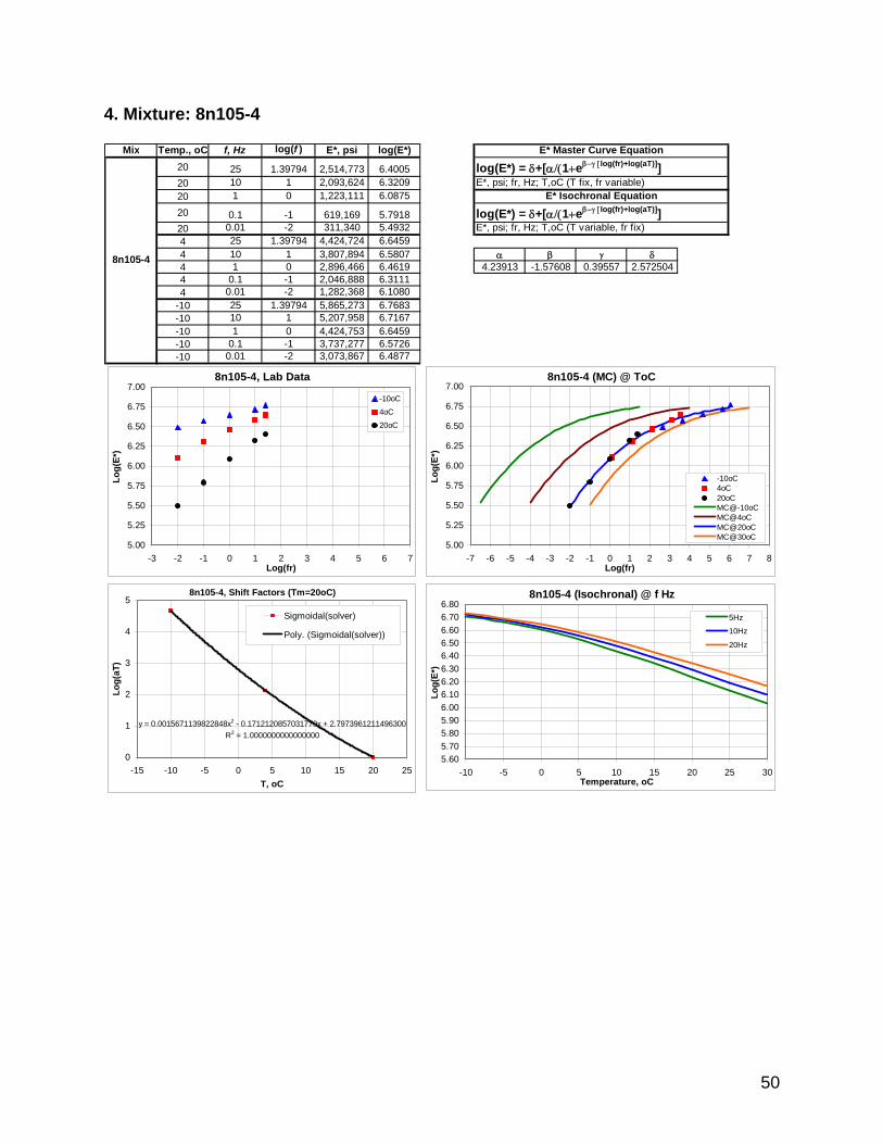
50
4. Mixture: 8n105-4
Mix Temp., oC f, Hz log(f ) E*, psi log(E*)20 25 1.39794 2,514,773 6.4005 log(E*) = δ+[α/(1+eβ−γ [log(fr)+log(aT)]]20 10 1 2,093,624 6.3209 E*, psi; fr, Hz; T,oC (T fix, fr variable)20 1 0 1,223,111 6.0875
20 0.1 -1 619,169 5.7918 log(E*) = δ+[α/(1+eβ−γ [log(fr)+log(aT)]]20 0.01 -2 311,340 5.4932 E*, psi; fr, Hz; T,oC (T variable, fr fix)4 25 1.39794 4,424,724 6.64594 10 1 3,807,894 6.5807 α β γ δ4 1 0 2,896,466 6.4619 4.23913 -1.57608 0.39557 2.5725044 0.1 -1 2,046,888 6.31114 0.01 -2 1,282,368 6.1080
-10 25 1.39794 5,865,273 6.7683-10 10 1 5,207,958 6.7167-10 1 0 4,424,753 6.6459-10 0.1 -1 3,737,277 6.5726-10 0.01 -2 3,073,867 6.4877
8n105-4
E* Master Curve Equation
E* Isochronal Equation
8n105-4 (MC) @ ToC
5.00
5.25
5.50
5.75
6.00
6.25
6.50
6.75
7.00
-7 -6 -5 -4 -3 -2 -1 0 1 2 3 4 5 6 7 8Log(fr)
Log(
E*)
-10oC4oC20oCMC@-10oCMC@4oCMC@20oCMC@30oC
8n105-4, Shift Factors (Tm=20oC)
y = 0.0015671139822848x2 - 0.1712120857031770x + 2.7973961211496300R2 = 1.0000000000000000
0
1
2
3
4
5
-15 -10 -5 0 5 10 15 20 25T, oC
Log(
aT)
Sigmoidal(solver)
Poly. (Sigmoidal(solver))
8n105-4, Lab Data
5.00
5.25
5.50
5.75
6.00
6.25
6.50
6.75
7.00
-3 -2 -1 0 1 2 3 4 5 6 7Log(fr)
Log(
E*)
-10oC
4oC20oC
8n105-4 (Isochronal) @ f Hz
5.605.705.805.906.006.106.206.306.406.506.606.706.80
-10 -5 0 5 10 15 20 25 30Temperature, oC
Log(
E*)
5Hz
10Hz
20Hz

51
5. Mixture: 8n70-4
Mix Temp., oC f, Hz log(f ) E*, psi log(E*)20 25 1.39794 2,796,652 6.4466 log(E*) = δ+[α/(1+eβ−γ [log(fr)+log(aT)]]20 10 1 2,100,721 6.3224 E*, psi; fr, Hz; T,oC (T fix, fr variable)20 1 0 1,223,436 6.0876
20 0.1 -1 468,047 5.6703 log(E*) = δ+[α/(1+eβ−γ [log(fr)+log(aT)]]20 0.01 -2 180,386 5.2562 E*, psi; fr, Hz; T,oC (T variable, fr fix)4 25 1.39794 4,644,180 6.66694 10 1 4,941,784 6.6939 α β γ δ4 1 0 3,561,333 6.5516 2.585328 -0.99722 0.667679 4.1770894 0.1 -1 2,308,503 6.36334 0.01 -2 1,210,738 6.0831
-10 25 1.39794 5,520,441 6.7420-10 10 1 4,880,778 6.6885-10 1 0 4,152,616 6.6183-10 0.1 -1 3,365,193 6.5270-10 0.01 -2 2,690,518 6.4298
8n70-4
E* Master Curve Equation
E* Isochronal Equation
8n70-4 (MC) @ ToC
5.0
5.3
5.5
5.8
6.0
6.3
6.5
6.8
7.0
-7 -6 -5 -4 -3 -2 -1 0 1 2 3 4 5 6 7Log(fr)
Log(
E*)
-10oC4oC20oCMC@20oCMC@30oCMC@4oCMC@-10oC
8n70-4, Shift Factors (Tm=20oC)
y = 0.112028258155584xR2 = 0.980156834329638
0
1
2
3
4
-5 0 5 10 15 20 25 30 35T, oC
Log(
aT)
Sigmoidal(solver)Linear (Sigmoidal(solver))
8n70-4, Lab Data
5.00
5.25
5.50
5.75
6.00
6.25
6.50
6.75
7.00
-3 -2 -1 0 1 2 3 4 5 6 7Log(fr)
Log(
E*)
-10oC
4oC20oC
8n70-4 (Isochronal) @ f Hz
5.705.805.906.006.106.206.306.406.506.606.706.806.90
-10 -5 0 5 10 15 20 25 30Temperature, oC
Log(
E*)
5Hz
10Hz
20Hz

52
6. Mixture: 5n90-4
Mix Temp., oC f, Hz log(f ) E*, psi log(E*)20 25 1.39794 2,281,908 6.3583 log(E*) = δ+[α/(1+eβ−γ [log(fr)+log(aT)]]20 10 1 1,939,538 6.2877 E*, psi; fr, Hz; T,oC (T fix, fr variable)20 1 0 1,303,231 6.1150
20 0.1 -1 681,402 5.8334 log(E*) = δ+[α/(1+eβ−γ [log(fr)+log(aT)]]20 0.01 -2 345,008 5.5378 E*, psi; fr, Hz; T,oC (T variable, fr fix)4 25 1.39794 4,302,466 6.63374 10 1 3,926,278 6.5940 α β γ δ4 1 0 3,205,892 6.5059 3.853232 -1.40771 0.372901 34 0.1 -1 2,419,913 6.38384 0.01 -2 1,684,885 6.2266
-10 25 1.39794 6,019,814 6.7796-10 10 1 5,555,593 6.7447-10 1 0 4,937,647 6.6935-10 0.1 -1 4,313,358 6.6348-10 0.01 -2 3,568,472 6.5525
5n90-4
E* Master Curve Equation
E* Isochronal Equation
5n90-4 (MC) @ ToC
5.00
5.25
5.50
5.75
6.00
6.25
6.50
6.75
7.00
-7 -6 -5 -4 -3 -2 -1 0 1 2 3 4 5 6 7 8Log(fr)
Log(
E*)
-10oC4oC20oCMC@-10oCMC@4oCMC@20oCMC@30oC
5n90-4, Shift Factors (Tm=20oC)
y = -3.11616677283015E-05x2 - 1.56799383507021E-01x + 3.14845233723176E+00
R2 = 1.00000000000000E+000
1
2
3
4
5
-15 -10 -5 0 5 10 15 20 25T, oC
Log(
aT)
Sigmoidal(solver)Poly. (Sigmoidal(solver))
5n90-4, Lab Data
5.00
5.25
5.50
5.75
6.00
6.25
6.50
6.75
7.00
-3 -2 -1 0 1 2 3 4 5 6 7Log(fr)
Log(
E*)
-10oC
4oC20oC
5n90-4 (Isochronal) @ f Hz
5.80
5.90
6.00
6.10
6.20
6.30
6.40
6.50
6.60
6.70
6.80
-10 -5 0 5 10 15 20 25 30Temperature, oC
Log(
E*)
5Hz
10Hz
20Hz

53
7. Mixture: 3n70-4
Mix Temp., oC f, Hz log(f ) E*, psi log(E*)20 25 1.39794 1,975,478 6.2957 log(E*) = δ+[α/(1+eβ−γ [log(fr)+log(aT)]]20 10 1 1,825,954 6.2615 E*, psi; fr, Hz; T,oC (T fix, fr variable)20 1 0 1,039,997 6.0170
20 0.1 -1 485,638 5.6863 log(E*) = δ+[α/(1+eβ−γ [log(fr)+log(aT)]]20 0.01 -2 230,360 5.3624 E*, psi; fr, Hz; T,oC (T variable, fr fix)4 25 1.39794 4,248,690 6.62834 10 1 3,812,914 6.5813 α β γ δ4 1 0 2,964,555 6.4720 15.89772 -2.74417 0.282251 -8.931564 0.1 -1 2,108,081 6.32394 0.01 -2 1,241,482 6.0939
-10 25 1.39794 6,641,237 6.8222-10 10 1 5,792,996 6.7629-10 1 0 4,410,943 6.6445-10 0.1 -1 3,945,896 6.5961-10 0.01 -2 3,264,364 6.5138
3n70-4
E* Master Curve Equation
E* Isochronal Equation
3n70-4 (MC) @ ToC
5.00
5.25
5.50
5.75
6.00
6.25
6.50
6.75
7.00
-7 -6 -5 -4 -3 -2 -1 0 1 2 3 4 5 6 7 8Log(fr)
Log(
E*)
-10oC4oC20oCMC@-10oCMC@4oCMC@20oCMC@30oC
3n70-4, Shift Factors (Tm=20oC)
y = 3.29817535739433E-04x2 - 1.59160341372851E-01x + 3.05127981316125E+00
R2 = 1.00000000000000E+000
1
2
3
4
5
-15 -10 -5 0 5 10 15 20 25T, oC
Log(
aT)
Sigmoidal(solver)Poly. (Sigmoidal(solver))
3n70-4, Lab Data
5.00
5.25
5.50
5.75
6.00
6.25
6.50
6.75
7.00
-3 -2 -1 0 1 2 3 4 5 6 7Log(fr)
Log(
E*)
-10oC
4oC20oC
3n70-4 (Isochronal) @ f Hz
5.80
5.90
6.00
6.10
6.20
6.30
6.40
6.50
6.60
6.70
6.80
-10 -5 0 5 10 15 20 25 30Temperature, oC
Log(
E*)
5Hz
10Hz
20Hz

54
8. Mixture: 3n90t-4
Mix Temp., oC f, Hz log(f ) E*, psi log(E*)20 25 1.39794 2,068,259 6.3156 log(E*) = δ+[α/(1+eβ−γ [log(fr)+log(aT)]]20 10 1 1,976,864 6.2960 E*, psi; fr, Hz; T,oC (T fix, fr variable)20 1 0 1,021,345 6.0092
20 0.1 -1 510,600 5.7081 log(E*) = δ+[α/(1+eβ−γ [log(fr)+log(aT)]]20 0.01 -2 246,215 5.3913 E*, psi; fr, Hz; T,oC (T variable, fr fix)4 25 1.39794 8,192,337 6.91344 10 1 7,856,894 6.8953 α β γ δ4 1 0 4,546,976 6.6577 309.8298 -5.67716 0.23495 -302.7564 0.1 -1 3,308,437 6.51964 0.01 -2 3,566,404 6.5522
-10 25 1.39794 6,423,955 6.8078-10 10 1 5,031,558 6.7017-10 1 0 4,285,049 6.6320-10 0.1 -1 3,415,170 6.5334-10 0.01 -2 2,974,523 6.4734
3n90t-4
E* Master Curve Equation
E* Isochronal Equation
3n90t-4 (MC) @ 20oC
4.0
4.5
5.0
5.5
6.0
6.5
7.0
-8 -7 -6 -5 -4 -3 -2 -1 0 1 2 3 4 5 6 7 8Log(fr)
Log(
E*)
-10oC4oC20oCMC@-10oCMC@4oCMC@20oCMC@30oC
3n90t-4, Shift Factors (Tm=20oC)
y = 0.179186773356285xR2 = 0.819438129966084
0
1
2
3
4
5
-5 0 5 10 15 20 25 30 35Tm-T, oC
Log(
aT)
Sigmoidal(solver)Linear (Sigmoidal(solver))
3n90t-4, Lab Data
5.00
5.25
5.50
5.75
6.00
6.25
6.50
6.75
7.00
-3 -2 -1 0 1 2 3 4 5 6 7Log(fr)
Log(
E*)
-10oC
4oC20oC
3n90t-4 (Isochronal) @ f Hz
5.705.805.906.006.106.206.306.406.506.606.706.806.90
-10 -5 0 5 10 15 20 25 30Temperature, oC
Log(
E*)
5Hz
10Hz
20Hz

55
9. Mixture: 6n50-4
Mix Temp., oC f, Hz log(f ) E*, psi log(E*)20 25 1.39794 2,160,317 6.3345 log(E*) = δ+[α/(1+eβ−γ [log(fr)+log(aT)]]20 10 1 1,814,456 6.2587 E*, psi; fr, Hz; T,oC (T fix, fr variable)20 1 0 958,310 5.9815
20 0.1 -1 429,480 5.6329 log(E*) = δ+[α/(1+eβ−γ [log(fr)+log(aT)]]20 0.01 -2 192,058 5.2834 E*, psi; fr, Hz; T,oC (T variable, fr fix)4 25 1.39794 3,874,051 6.58824 10 1 3,559,361 6.5514 α β γ δ4 1 0 2,578,673 6.4114 2.461637 -0.86032 0.595743 4.2507794 0.1 -1 1,699,073 6.23024 0.01 -2 922,401 5.9649
-10 25 1.39794 4,729,470 6.6748-10 10 1 4,424,406 6.6459-10 1 0 3,751,861 6.5742-10 0.1 -1 3,123,464 6.4946-10 0.01 -2 2,381,351 6.3768
6n50-4
E* Master Curve Equation
E* Isochronal Equation
6n50-4 (MC) @ ToC
5.00
5.25
5.50
5.75
6.00
6.25
6.50
6.75
7.00
-7 -6 -5 -4 -3 -2 -1 0 1 2 3 4 5 6 7 8Log(fr)
Log(
E*)
-10oC4oC20oCMC@-10oCMC@4oCMC@20oCMC@30oC
6n50-4, Shift Factors (Tm=20oC)
y = -6.92615463100850E-05x2 - 1.19535455899662E-01x + 2.41841373651727E+00
R2 = 9.99999999999999E-01
0
1
2
3
4
-15 -10 -5 0 5 10 15 20 25T, oC
Log(
aT)
Sigmoidal(solver)Poly. (Sigmoidal(solver))
6n50-4, Lab Data
5.00
5.25
5.50
5.75
6.00
6.25
6.50
6.75
7.00
-3 -2 -1 0 1 2 3 4 5 6 7Log(fr)
Log(
E*)
-10oC
4oC20oC
6n50-4 (Isochronal) @ f Hz
5.605.705.805.906.006.106.206.306.406.506.606.706.80
-10 -5 0 5 10 15 20 25 30Temperature, oC
Log(
E*)
5Hz
10Hz
20Hz

56
10. Mixture: 1n105-4
Mix Temp., oC f, Hz log(f ) E*, psi log(E*)20 25 1.39794 2,640,970 6.4218 log(E*) = δ+[α/(1+eβ−γ [log(fr)+log(aT)]]20 10 1 2,169,385 6.3363 E*, psi; fr, Hz; T,oC (T fix, fr variable)20 1 0 1,285,470 6.1091
20 0.1 -1 639,656 5.8059 log(E*) = δ+[α/(1+eβ−γ [log(fr)+log(aT)]]20 0.01 -2 355,026 5.5503 E*, psi; fr, Hz; T,oC (T variable, fr fix)4 25 1.39794 4,391,011 6.64264 10 1 3,855,558 6.5861 α β γ δ4 1 0 2,956,339 6.4708 2.252721 -0.85839 0.531406 4.527694 0.1 -1 2,106,860 6.32364 0.01 -2 1,334,580 6.1253
-10 25 1.39794 5,738,162 6.7588-10 10 1 5,010,373 6.6999-10 1 0 4,273,693 6.6308-10 0.1 -1 3,652,676 6.5626-10 0.01 -2 3,144,618 6.4976
1n105-4
E* Master Curve Equation
E* Isochronal Equation
1n105-4 (MC) @ ToC
5.00
5.25
5.50
5.75
6.00
6.25
6.50
6.75
7.00
-7 -6 -5 -4 -3 -2 -1 0 1 2 3 4 5 6 7 8Log(fr)
Log(
E*)
-10oC4oC20oCMC@-10oCMC@4oCMC@20oCMC@30oC
1n105-4, Shift Factors (Tm=20oC)
y = 1.66091860896915E-04x2 - 1.28403168947947E-01x + 2.50162663460019E+00
R2 = 1.00000000000000E+000
1
2
3
4
-15 -10 -5 0 5 10 15 20 25T, oC
Log(
aT)
Sigmoidal(solver)Poly. (Sigmoidal(solver))
1n105-4, Lab Data
5.00
5.25
5.50
5.75
6.00
6.25
6.50
6.75
7.00
-3 -2 -1 0 1 2 3 4 5 6 7Log(fr)
Log(
E*)
-10oC
4oC20oC
1n105-4 (Isochronal) @ f Hz
5.605.705.805.906.006.106.206.306.406.506.606.706.80
-10 -5 0 5 10 15 20 25 30Temperature, oC
Log(
E*)
5Hz
10Hz
20Hz

57
11. Mixture: 2n90-4
Mix Temp., oC f, Hz log(f ) E*, psi log(E*)20 25 1.39794 2,176,844 6.3378 log(E*) = δ+[α/(1+eβ−γ [log(fr)+log(aT)]]20 10 1 1,916,995 6.2826 E*, psi; fr, Hz; T,oC (T fix, fr variable)20 1 0 1,201,324 6.0797
20 0.1 -1 648,415 5.8119 log(E*) = δ+[α/(1+eβ−γ [log(fr)+log(aT)]]20 0.01 -2 336,861 5.5275 E*, psi; fr, Hz; T,oC (T variable, fr fix)4 25 1.39794 4,244,625 6.62784 10 1 3,749,350 6.5740 α β γ δ4 1 0 2,930,450 6.4669 2.74181 -0.86852 0.427431 4.149784 0.1 -1 2,255,820 6.35334 0.01 -2 1,519,280 6.1816
-10 25 1.39794 5,900,112 6.7709-10 10 1 5,157,912 6.7125-10 1 0 7,053,765 6.8484-10 0.1 -1 5,031,887 6.7017-10 0.01 -2 3,133,969 6.4961
2n90-4
E* Master Curve Equation
E* Isochronal Equation
2n90-4 (MC) @ ToC
5.00
5.25
5.50
5.75
6.00
6.25
6.50
6.75
7.00
-7 -6 -5 -4 -3 -2 -1 0 1 2 3 4 5 6 7 8Log(fr)
Log(
E*)
-10oC4oC20oCMC@-10CMC@4oCMC@20oCMC@30oC
2n90-4, Shift Factors (Tm=20oC)
y = 0.0000736265911921944x2 - 0.1394908453214830000x + 2.7603662699527800000
R2 = 0.9999999999999980000
0
1
2
3
4
5
-15 -10 -5 0 5 10 15 20 25T, oC
Log(
aT)
Sigmoidal(solver)Poly. (Sigmoidal(solver))
2n90-4, Lab Data
5.00
5.25
5.50
5.75
6.00
6.25
6.50
6.75
7.00
-3 -2 -1 0 1 2 3 4 5 6 7Log(fr)
Log(
E*)
-10oC
4oC20oC
2n90-4 (Isochronal) @ f Hz
5.605.705.805.906.006.106.206.306.406.506.606.706.80
-10 -5 0 5 10 15 20 25 30Temperature, oC
Log(
E*)
5Hz
10Hz
20Hz

58
12. Mixture: 3n90-4
Mix Temp., oC f, Hz log(f ) E*, psi log(E*)20 25 1.39794 2,545,833 6.4058 log(E*) = δ+[α/(1+eβ−γ [log(fr)+log(aT)]]20 10 1 2,413,540 6.3827 E*, psi; fr, Hz; T,oC (T fix, fr variable)20 1 0 1,622,904 6.2103
20 0.1 -1 912,069 5.9600 log(E*) = δ+[α/(1+eβ−γ [log(fr)+log(aT)]]20 0.01 -2 453,035 5.6561 E*, psi; fr, Hz; T,oC (T variable, fr fix)4 25 1.39794 3,805,931 6.58054 10 1 3,773,279 6.5767 α β γ δ4 1 0 3,108,120 6.4925 3.794327 -1.68927 0.416549 34 0.1 -1 2,448,941 6.38904 0.01 -2 1,740,684 6.2407
-10 25 1.39794 4,592,852 6.6621-10 10 1 6,267,122 6.7971-10 1 0 5,451,552 6.7365-10 0.1 -1 4,991,356 6.6982-10 0.01 -2 4,028,589 6.6052
3n90-4
E* Master Curve Equation
E* Isochronal Equation
3n90-4 (MC) @ T oC
5.00
5.25
5.50
5.75
6.00
6.25
6.50
6.75
7.00
-7 -6 -5 -4 -3 -2 -1 0 1 2 3 4 5 6 7 8Log(fr)
Log(
E*)
-10oC4oC20oCMC@-10oCMC@4oCMC@20oCMC@30oC
3n90-4, Shift Factors (Tm=20oC)
y = 2.20653538054395E-03x2 - 1.78922238781753E-01x + 2.69583062341748E+00
R2 = 9.99999999999998E-010
1
2
3
4
5
-15 -10 -5 0 5 10 15 20 25T, oC
Log(
aT)
Sigmoidal(solver)Poly. (Sigmoidal(solver))
3n90-4, Lab Data
5.00
5.25
5.50
5.75
6.00
6.25
6.50
6.75
7.00
-3 -2 -1 0 1 2 3 4 5 6 7Log(fr)
Log(
E*)
-10oC4oC
20oC
3n90-4 (Isochronal) @ f Hz
6.00
6.10
6.20
6.30
6.40
6.50
6.60
6.70
6.80
-10 -5 0 5 10 15 20 25 30Temperature, oC
Log(
E*)
5Hz
10Hz
20Hz

59
13. Mixture: 5n105-4
Mix Temp., oC f, Hz log(f ) E*, psi log(E*)20 25 1.39794 1,313,207 6.1183 log(E*) = δ+[α/(1+eβ−γ [log(fr)+log(aT)]]20 10 1 1,014,643 6.0063 E*, psi; fr, Hz; T,oC (T fix, fr variable)20 1 0 551,022 5.7412
20 0.1 -1 258,590 5.4126 log(E*) = δ+[α/(1+eβ−γ [log(fr)+log(aT)]]20 0.01 -2 150,071 5.1763 E*, psi; fr, Hz; T,oC (T variable, fr fix)4 25 1.39794 2,946,520 6.46934 10 1 2,507,654 6.3993 α β γ δ4 1 0 1,746,962 6.2423 2.200624 -0.34473 0.523833 4.4354344 0.1 -1 1,028,602 6.01224 0.01 -2 559,848 5.7481
-10 25 1.39794 3,992,619 6.6013-10 10 1 3,608,442 6.5573-10 1 0 3,004,031 6.4777-10 0.1 -1 2,421,586 6.3841-10 0.01 -2 1,754,003 6.2440
5n105-4
E* Master Curve Equation
E* Isochronal Equation
5n105-4 (MC) @ ToC
5.00
5.25
5.50
5.75
6.00
6.25
6.50
6.75
7.00
-7 -6 -5 -4 -3 -2 -1 0 1 2 3 4 5 6 7 8Log(fr)
Log(
E*)
-10oC4oC20oCMC@-10oCMC@4oCMC@20oCMC@30oC
5n105-4, Shift Factors (Tm=20oC)
y = 1.40073535862098E-03x2 - 1.69616722746523E-01x + 2.83204031148207E+00
R2 = 9.99999999999999E-010
1
2
3
4
5
-15 -10 -5 0 5 10 15 20 25T, oC
Log(
aT)
Sigmoidal(solver)Poly. (Sigmoidal(solver))
5n105-4, Lab Data
5.00
5.25
5.50
5.75
6.00
6.25
6.50
6.75
7.00
-3 -2 -1 0 1 2 3 4 5 6 7Log(fr)
Log(
E*)
-10oC
4oC20oC
5n105-4 (Isochronal) @ f Hz
5.60
5.70
5.80
5.90
6.00
6.10
6.20
6.30
6.40
6.50
6.60
-10 -5 0 5 10 15 20 25 30Temperature, oC
Log(
E*)
5Hz
10Hz
20Hz

60
14. Mixture: 6n50s-4
Mix Temp., oC f, Hz log(f ) E*, psi log(E*)20 25 1.39794 1,685,893 6.2268 log(E*) = δ+[α/(1+eβ−γ [log(fr)+log(aT)]]20 10 1 1,414,865 6.1507 E*, psi; fr, Hz; T,oC (T fix, fr variable)20 1 0 842,049 5.9253
20 0.1 -1 429,617 5.6331 log(E*) = δ+[α/(1+eβ−γ [log(fr)+log(aT)]]20 0.01 -2 231,310 5.3642 E*, psi; fr, Hz; T,oC (T variable, fr fix)4 25 1.39794 5,704,769 6.75624 10 1 5,391,418 6.7317 α β γ δ4 1 0 3,536,090 6.5485 1.996327 0.159603 0.59538 4.971274 0.1 -1 2,202,615 6.34294 0.01 -2 1,103,557 6.0428
-10 25 1.39794 7,176,677 6.8559-10 10 1 8,883,851 6.9486-10 1 0 6,819,045 6.8337-10 0.1 -1 4,767,024 6.6782-10 0.01 -2 4,946,339 6.6943
6n50s-4
E* Master Curve Equation
E* Isochronal Equation
6n50s-4 (MC) @ ToC
5.00
5.25
5.50
5.75
6.00
6.25
6.50
6.75
7.00
-7 -6 -5 -4 -3 -2 -1 0 1 2 3 4 5 6 7 8Log(fr)
Log(
E*)
-10oC4oC20oCMC@-10oCMC@4oCMC@20oCMC@30oC
6n50s-4, Shift Factors (Tm=20oC)
y = -0.000189322553931694x2 - 0.154224959385601000x + 3.160228209284700000
R2 = 0.9999999999999990000
1
2
3
4
5
-15 -10 -5 0 5 10 15 20 25T, oC
Log(
aT)
Sigmoidal(solver)Poly. (Sigmoidal(solver))
6n50s-4, Lab Data
5.00
5.25
5.50
5.75
6.00
6.25
6.50
6.75
7.00
-3 -2 -1 0 1 2 3 4 5 6 7Log(fr)
Log(
E*)
-10oC
4oC20oC
6n50s-4 (Isochronal) @ f Hz
5.605.705.805.906.006.106.206.306.406.506.606.706.806.907.00
-10 -5 0 5 10 15 20 25 30Temperature, oC
Log(
E*)
5Hz
10Hz
20Hz

61
15. Mixture: 1n80d-4
Mix Temp., oC f, Hz log(f ) E*, psi log(E*)20 25 1.39794 1,728,348 6.2376 log(E*) = δ+[α/(1+eβ−γ [log(fr)+log(aT)]]20 10 1 1,316,114 6.1193 E*, psi; fr, Hz; T,oC (T fix, fr variable)20 1 0 683,694 5.8349
20 0.1 -1 334,867 5.5249 log(E*) = δ+[α/(1+eβ−γ [log(fr)+log(aT)]]20 0.01 -2 182,619 5.2615 E*, psi; fr, Hz; T,oC (T variable, fr fix)4 25 1.39794 3,028,375 6.48124 10 1 2,513,515 6.4003 α β γ δ4 1 0 1,681,448 6.2257 2.173292 -0.42391 0.561721 4.5329564 0.1 -1 997,818 5.99914 0.01 -2 539,444 5.7319
-10 25 1.39794 4,353,652 6.6389-10 10 1 4,087,058 6.6114-10 1 0 3,131,745 6.4958-10 0.1 -1 2,537,390 6.4044-10 0.01 -2 1,841,579 6.2652
E* Master Curve Equation
E* Isochronal Equation
1n80d-4
1n80d-4 (MC) @ ToC
5.00
5.25
5.50
5.75
6.00
6.25
6.50
6.75
7.00
-7 -6 -5 -4 -3 -2 -1 0 1 2 3 4 5 6 7Log(fr)
Log(
E*)
-10oC4oC20oCMC@-10oCMC@4oCMC@20oCMC@30oC
1n80d-4, Shift Factors (Tm=20oC)
y = 1.56280875778826E-03x2 - 1.35155748004656E-01x + 2.07799145697781E+00
R2 = 9.99999999999998E-010
1
2
3
4
-15 -10 -5 0 5 10 15 20 25T, oC
Log(
aT)
Sigmoidal(solver)Poly. (Sigmoidal(solver))
1n80d-4, Lab Data
5.00
5.25
5.50
5.75
6.00
6.25
6.50
6.75
7.00
-3 -2 -1 0 1 2 3 4 5 6 7Log(fr)
Log(
E*)
-10oC
4oC20oC
1n80d-4 (Isochronal) @ f Hz
5.80
5.90
6.00
6.10
6.20
6.30
6.40
6.50
6.60
6.70
6.80
-10 -5 0 5 10 15 20 25 30Temperature, oC
Log(
E*)
5Hz
10Hz
20Hz
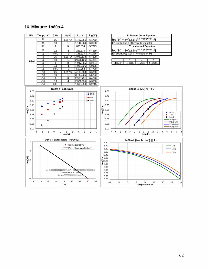
62
16. Mixture: 1n80s-4
Mix Temp., oC f, Hz log(f ) E*, psi log(E*)20 25 1.39794 1,497,066 6.1752 log(E*) = δ+[α/(1+eβ−γ [log(fr)+log(aT)]]20 10 1 1,144,864 6.0588 E*, psi; fr, Hz; T,oC (T fix, fr variable)20 1 0 606,594 5.7829
20 0.1 -1 286,335 5.4569 log(E*) = δ+[α/(1+eβ−γ [log(fr)+log(aT)]]20 0.01 -2 156,120 5.1935 E*, psi; fr, Hz; T,oC (T variable, fr fix)4 25 1.39794 3,039,138 6.48284 10 1 2,661,126 6.4251 α β γ δ4 1 0 1,947,205 6.2894 2.155301 -0.33317 0.576007 4.5264644 0.1 -1 1,088,026 6.03664 0.01 -2 599,758 5.7780
-10 25 1.39794 4,198,003 6.6230-10 10 1 3,743,306 6.5733-10 1 0 2,968,791 6.4726-10 0.1 -1 2,321,535 6.3658-10 0.01 -2 1,665,259 6.2215
E* Master Curve Equation
E* Isochronal Equation
1n80s-4
1n80s-4 (MC) @ ToC
5.00
5.25
5.50
5.75
6.00
6.25
6.50
6.75
7.00
-7 -6 -5 -4 -3 -2 -1 0 1 2 3 4 5 6 7 8Log(fr)
Log(
E*)
-10oC4oC20oCMC@-10oCMC@4oCMC@20oCMC@30oC
1n80s-4, Shift Factors (Tm=20oC)
y = -0.000215003227961743x2 - 0.117377060066726000x + 2.433542492519230000
R2 = 0.999999999999998000
0
1
2
3
4
-15 -10 -5 0 5 10 15 20 25T, oC
Log(
aT)
Sigmoidal(solver)Poly. (Sigmoidal(solver))
1n80s-4, Lab Data
5.00
5.25
5.50
5.75
6.00
6.25
6.50
6.75
7.00
-3 -2 -1 0 1 2 3 4 5 6 7Log(fr)
Log(
E*)
-10oC
4oC20oC
1n80s-4 (Isochronal) @ f Hz
5.605.705.805.906.006.106.206.306.406.506.606.706.80
-10 -5 0 5 10 15 20 25 30Temperature, oC
Log(
E*)
5Hz
10Hz
20Hz

63
APPENDIX B

64
1. Binder: B1 (SBS 70-22)
Binder 1 (PG70-22), MC
0
1
2
3
4
5
6
7
8
-7.0 -6.0 -5.0 -4.0 -3.0 -2.0 -1.0 0.0 1.0 2.0log(fr), Hz
log(
G*)
, Pa 16oC
21.9oC27.9oC34oC40oC46.1oC52.1oC58.1oC64.1oC70.1oC76.1oC82.1oCFit Eq. 21.9oCM.C. 20oCM.C. 30oCM.C. 40oC
Binder 1 (PG70-22), MC
y = -0.235023699947405x3 - 1.819118259654220x2 - 6.337179694963530x + 57.899470195739900R2 = 0.938271139928102
30
40
50
60
70
80
90
-7.0 -6.0 -5.0 -4.0 -3.0 -2.0 -1.0 0.0 1.0 2.0log(fr), Hz
Phas
e A
ngle
, Deg
ree
82.1oC76.1oC70.1oC64.1oC58.1oC52.1oC46.1oC40oC(H)[email protected]
Binder 1 (PG70-22), Shift Factor Fit
y = 0.000628665982156308x2 - 0.144621810061204000x + 2.857081958570830000R2 = 0.999903494136514000
-5.0
-4.5
-4.0
-3.5
-3.0
-2.5
-2.0
-1.5
-1.0
-0.5
0.0
0.5
1.0
10 20 30 40 50 60 70 80 90Temperature, oC
log(
a[T]
)
Binder 1 (PG70-22), Black Space
y = -0.692813039762541x3 + 9.039082857848860x2 - 41.371403366596200x + 132.760730661917000R2 = 0.939890801114808
30
40
50
60
70
80
90
1.0 2.0 3.0 4.0 5.0 6.0 7.0 8.0log(G*), Pa
Phas
e A
ngle
, Deg
ree
82.1oC76.1oC70.1oC64.1oC58.1oC52.1oC46.1oC40oC(H)34oC27.9oC21.9oC16oCPoly. (G*/P.A.)
Binder 1 (PG70-22), Complex Planey = 0.001558838799536x2 + 0.902242876320453x + 0.729919071563186
R2 = 0.998823984097622
0
1
2
3
4
5
6
7
8
0 1 2 3 4 5 6 7 8
log(G'), Pa
log(
G")
, Pa
G'vs.G"Poly. (G'vs.G")
Binder 1 (PG70-22), Isochronal
1.E+03
1.E+04
1.E+05
1.E+06
1.E+07
1.E+08
0 10 20 30 40 50 60 70 80 90 100Temperature, oC
G*,
Pa
20 Hz
15 Hz
10 Hz
5 Hz
log(a[T]) = a * T2 + b * T +c log(G*) = A * (log(fr)+log(a[T]))2 + B * (log(fr)+log(a[T])) + C log(G*) = A * (log(fr)+log(a[T]))2 + B * (log(fr)+log(a[T])) + CT, oC G*, Pa; fr, Hz; T,oC (T fix, fr variable) G*, Pa; fr, Hz; T,oC (fr fix, T variable)
log(δ) = W * (log(fr)+log(a[T]))3 + X * (log(fr)+log(a[T]))2 + Y * (log(fr)+log(a[T])) + Zδ, degree; fr, Hz; T, oC
G* Master Curve Equation G* Isochronal Equation
δ Master Curve Equation
Shift Factor Equation
A B C a b c-0.01730557 0.635534613 6.303634486 0.000628666 -0.14462181 2.857081959
W X Y Z-0.23502370 -1.81911826 -6.33717969 57.8994702
G* Master Curve Coefficients, Pa Shift Factor Coefficients
δ Master Curve Coefficients, degree

65
2. Binder: B2 (64-22)
Binder 2 (PG64-22), MC
0
1
2
3
4
5
6
7
8
-7.0 -6.0 -5.0 -4.0 -3.0 -2.0 -1.0 0.0 1.0 2.0log(fr), Hz
log(
G*)
, Pa 16oC
21.9oC27.9oC34oC46.1oC52.1oC58.1oC64.1oC70.1oCFit Eq. 21.9oCM.C. 20oCM.C. 30oCM.C. 40oC
Binder 2 (PG64-22), MC
y = 0.0979430072858065x3 - 0.1203941834595860x2 - 8.8103340656857500x + 59.1259137055026000R2 = 0.9949220545264180
30
40
50
60
70
80
90
-7.0 -6.0 -5.0 -4.0 -3.0 -2.0 -1.0 0.0 1.0 2.0log(fr), Hz
Phas
e A
ngle
, Deg
ree
70.1oC
64.1oC
58.1oC
52.1oC
46.1oC
34oC
27.9oC
21.9oC
16oC
Shifted
Binder 2 (PG64-22), Shift Factor Fit
y = 0.000729409566405589x2 - 0.154572556037350000x + 3.037408250521600000R2 = 0.999987290254177000
-5.0
-4.5
-4.0
-3.5
-3.0
-2.5
-2.0
-1.5
-1.0
-0.5
0.0
0.5
1.0
10 20 30 40 50 60 70 80 90Temperature, oC
log(
a[T]
)
Binder 2 (PG64-22), Black Space
y = -0.0191816158907727x3 - 1.3257008436078600x2 + 5.7214125577730500x + 81.9485117199801000R2 = 0.9946309346906100
30
40
50
60
70
80
90
1.0 2.0 3.0 4.0 5.0 6.0 7.0 8.0log(G*), Pa
Phas
e A
ngle
, Deg
ree
70.1oC
64.1oC
58.1oC
52.1oC
46.1oC
34oC
27.9oC
21.9oC
16oC
Poly. (G*/P.A.)
Binder 2 (PG64-22), Complex Planey = 0.006013029221162x2 + 0.722847214602704x + 1.688108495894500
R2 = 0.999318256139701
0
1
2
3
4
5
6
7
8
0 1 2 3 4 5 6 7 8
log(G'), Pa
log(
G")
, Pa
G'vs.G"Poly. (G'vs.G")
Binder 2 (PG64-22), Isochronal
1.E+03
1.E+04
1.E+05
1.E+06
1.E+07
1.E+08
0 10 20 30 40 50 60 70 80 90 100Temperature, oC
G*,
Pa
20 Hz
15 Hz
10 Hz
5 Hz
log(a[T]) = a * T2 + b * T +c log(G*) = A * (log(fr)+log(a[T]))2 + B * (log(fr)+log(a[T])) + C log(G*) = A * (log(fr)+log(a[T]))2 + B * (log(fr)+log(a[T])) + CT, oC G*, Pa; fr, Hz; T,oC (T fix, fr variable) G*, Pa; fr, Hz; T,oC (fr fix, T variable)
log(δ) = W * (log(fr)+log(a[T]))3 + X * (log(fr)+log(a[T]))2 + Y * (log(fr)+log(a[T])) + Zδ, degree; fr, Hz; T, oC
Shift Factor Equation G* Master Curve Equation G* Isochronal Equation
δ Master Curve Equation
A B C a b c-0.038957 0.652824375 6.40582614 0.00072941 -0.15457256 3.037408251
W X Y Z0.09794301 -0.12039418 -8.81033407 59.1259137
δ Master Curve Coefficients, degree
G* Master Curve Coefficients, Pa Shift Factor Coefficients

66
3. Binder: B3 (64-22)
Binder 3 (PG64-22), MC
0
1
2
3
4
5
6
7
8
-7.0 -6.0 -5.0 -4.0 -3.0 -2.0 -1.0 0.0 1.0 2.0log(fr), Hz
log(
G*)
, Pa 16oC
21.9oC27.9oC34oC40oC46.1oC52.1oC58.1oC64.1oC70.1oCFit Eq. 21.9oCM.C. 20oCM.C. 30oCM.C. 40oC
Binder 3 (PG64-22), MC
y = 0.104087311244200x3 - 0.093699501205928x2 - 8.832524196619030x + 59.576875969747300R2 = 0.992834945675811
30
40
50
60
70
80
90
-7.0 -6.0 -5.0 -4.0 -3.0 -2.0 -1.0 0.0 1.0 2.0log(fr), Hz
Phas
e A
ngle
, Deg
ree
70.1oC
64.1oC
58.1oC
52.1oC
46.1oC
40oC(H)
34oC
27.9oC
21.9oC
16oC
Shifted
Binder 3 (PG64-22), Shift Factor Fit
y = 0.000696391666554x2 - 0.149357527211487x + 2.929601683537030R2 = 0.999897448004587
-5.0
-4.5
-4.0
-3.5
-3.0
-2.5
-2.0
-1.5
-1.0
-0.5
0.0
0.5
1.0
10 20 30 40 50 60 70 80 90Temperature, oC
log(
a[T]
)
Binder 3 (PG64-22), Black Space
y = -0.018651809223400x3 - 1.316527042239140x2 + 5.422908892554550x + 83.018569223339700R2 = 0.992441154958506
30
40
50
60
70
80
90
1.0 2.0 3.0 4.0 5.0 6.0 7.0 8.0log(G*), Pa
Phas
e A
ngle
, Deg
ree
70.1oC
64.1oC
58.1oC
52.1oC
46.1oC
40oC(H)
34oC
27.9oC
21.9oC
16oC
Poly. (G*/P.A.)
Binder 3 (PG64-22), Complex Planey = 0.010568394882174x2 + 0.678644726934739x + 1.784675583733980
R2 = 0.999160254382915
0
1
2
3
4
5
6
7
8
0 1 2 3 4 5 6 7 8log(G'), Pa
log(
G")
, Pa
G'vs.G"Poly. (G'vs.G")
Binder 3 (PG64-22), Isochronal
1.E+03
1.E+04
1.E+05
1.E+06
1.E+07
1.E+08
0 10 20 30 40 50 60 70 80 90 100Temperature, oC
G*,
Pa
20 Hz
15 Hz
10 Hz
5 Hz
log(a[T]) = a * T2 + b * T +c log(G*) = A * (log(fr)+log(a[T]))2 + B * (log(fr)+log(a[T])) + C log(G*) = A * (log(fr)+log(a[T]))2 + B * (log(fr)+log(a[T])) + CT, oC G*, Pa; fr, Hz; T,oC (T fix, fr variable) G*, Pa; fr, Hz; T,oC (fr fix, T variable)
log(δ) = W * (log(fr)+log(a[T]))3 + X * (log(fr)+log(a[T]))2 + Y * (log(fr)+log(a[T])) + Zδ, degree; fr, Hz; T, oC
Shift Factor Equation G* Master Curve Equation G* Isochronal Equation
δ Master Curve Equation
A B C a b c-0.03931266 0.661328483 6.348184178 0.000696392 -0.14935753 2.929601684
W X Y Z0.10408731 -0.09369950 -8.83252420 59.5768760
δ Master Curve Coefficients, degree
G* Master Curve Coefficients, Pa Shift Factor Coefficients

67
4. Binder: B4 (SBS 76-28)
Binder 4 (PG76-28), MC
0
1
2
3
4
5
6
7
8
-7.0 -6.0 -5.0 -4.0 -3.0 -2.0 -1.0 0.0 1.0 2.0log(fr), Hz
log(
G*)
, Pa 16oC
21.9oC27.9oC34oC40oC46.1oC52.1oC58.1oC64.1oC70.1oC76.1oC82.1oCFit Eq. 21.9oCM.C. 20oCM.C. 30oCM.C. 40oC
Binder 4 (PG76-28), MC
y = -0.356387809079251x3 - 2.446938025262320x2 - 2.715052808514000x + 57.796437686439500R2 = 0.537118999638008
30
40
50
60
70
80
90
-7.0 -6.0 -5.0 -4.0 -3.0 -2.0 -1.0 0.0 1.0 2.0log(fr), Hz
Phas
e A
ngle
, Deg
ree
82.1oC76.1oC70.1oC64.1oC58.1oC52.1oC46.1oC40oC(H)34oC27.9oC21.9oC16oCShiftedPoly. (Shifted)
Binder 4 (PG76-28), Shift Factor Fit
y = 0.000638412824286x2 - 0.143309626320639x + 2.812452802375360R2 = 0.999503946088308
-5.0
-4.5
-4.0
-3.5
-3.0
-2.5
-2.0
-1.5
-1.0
-0.5
0.0
0.5
1.0
10 20 30 40 50 60 70 80 90Temperature, oC
log(
a[T]
)
Binder 4 (PG76-28), Black Space
y = -1.608416642699690x3 + 22.109810560239800x2 - 96.527394770812500x + 188.350370270006000R2 = 0.543696579054905
30
40
50
60
70
80
90
1.0 2.0 3.0 4.0 5.0 6.0 7.0 8.0log(G*), Pa
Phas
e A
ngle
, Deg
ree
82.1oC76.1oC70.1oC64.1oC58.1oC52.1oC46.1oC40oC(H)34oC27.9oC21.9oC16oCPoly. (G*/P.A.)
Binder 4 (PG76-22), Complex Plane
y = 0.000843973232339x2 + 1.011072406423870x + 0.093437009967077R2 = 0.997866816333861
0
1
2
3
4
5
6
7
8
0 1 2 3 4 5 6 7 8
log(G'), Pa
log(
G")
, Pa
G'vs.G"Poly. (G'vs.G")
Binder 4 (PG76-28), Isochronal
1.E+03
1.E+04
1.E+05
1.E+06
1.E+07
1.E+08
0 10 20 30 40 50 60 70 80 90 100Temperature, oC
G*,
Pa
20 Hz
15 Hz
10 Hz
5 Hz
log(a[T]) = a * T2 + b * T +c log(G*) = A * (log(fr)+log(a[T]))2 + B * (log(fr)+log(a[T])) + C log(G*) = A * (log(fr)+log(a[T]))2 + B * (log(fr)+log(a[T])) + CT, oC G*, Pa; fr, Hz; T,oC (T fix, fr variable) G*, Pa; fr, Hz; T,oC (fr fix, T variable)
log(δ) = W * (log(fr)+log(a[T]))3 + X * (log(fr)+log(a[T]))2 + Y * (log(fr)+log(a[T])) + Zδ, degree; fr, Hz; T, oC
Shift Factor Equation G* Master Curve Equation G* Isochronal Equation
δ Master Curve Equation
A B C a b c0.00384471 0.6224636 5.969110789 0.000638413 -0.14330963 2.812452802
W X Y Z-0.35638781 -2.44693803 -2.71505281 57.7964377
δ Master Curve Coefficients, degree
G* Master Curve Coefficients, Pa Shift Factor Coefficients

68
5. Binder: B5 (SBS 76-22)
Binder 5 (PG76-22), MC
0
1
2
3
4
5
6
7
8
-7.0 -6.0 -5.0 -4.0 -3.0 -2.0 -1.0 0.0 1.0 2.0log(fr), Hz
log(
G*)
, Pa 16oC
21.9oC27.9oC34oC40oC46.1oC52.1oC58.1oC64.1oC70.1oC76.1oC82.1oCFit Eq. 21.9oCM.C. 20oCM.C. 30oCM.C. 40oC
Binder 5 (PG76-22), Shift Factor Fit
y = 0.000658306163851624x2 - 0.148388213233597000x + 2.914229975418430000R2 = 0.999710261734039000
-5.0
-4.5
-4.0
-3.5
-3.0
-2.5
-2.0
-1.5
-1.0
-0.5
0.0
0.5
1.0
10 20 30 40 50 60 70 80 90Temperature, oC
log(
a[T]
)
Binder 5 (PG76-22), MC
y = -0.267850732092370x3 - 2.187796013688250x2 - 5.524978343433560x + 57.109034221614300R2 = 0.790138977654779
30
40
50
60
70
80
90
-7.0 -6.0 -5.0 -4.0 -3.0 -2.0 -1.0 0.0 1.0 2.0log(fr), Hz
Phas
e A
ngle
, Deg
ree
82.1oC76.1oC70.1oC64.1oC58.1oC52.1oC46.1oC40oC(H)[email protected]
Binder 5 (PG76-22), Black Space
y = -0.981598074124804x3 + 13.219714851036000x2 - 58.507358559033800x + 146.442008974787000R2 = 0.798946546547083
30
40
50
60
70
80
90
1.0 2.0 3.0 4.0 5.0 6.0 7.0 8.0log(G*), Pa
Phas
e A
ngle
, Deg
ree
82.1oC76.1oC70.1oC64.1oC58.1oC52.1oC46.1oC40oC(H)34oC27.9oC21.9oC16oCPoly. (G*/P.A.)
Binder 5 (PG76-22), Complex Planey = -0.007830951723268x2 + 1.033855342941130x + 0.262369343672045
R2 = 0.998840057201241
0
1
2
3
4
5
6
7
8
0 1 2 3 4 5 6 7 8
log(G'), Pa
log(
G")
, Pa
G'vs.G"Poly. (G'vs.G")
Binder 5 (PG76-22), Isochronal
1.E+03
1.E+04
1.E+05
1.E+06
1.E+07
1.E+08
0 10 20 30 40 50 60 70 80 90 100Temperature, oC
G*,
Pa
20 Hz
15 Hz
10 Hz
5 Hz
log(a[T]) = a * T2 + b * T +c log(G*) = A * (log(fr)+log(a[T]))2 + B * (log(fr)+log(a[T])) + C log(G*) = A * (log(fr)+log(a[T]))2 + B * (log(fr)+log(a[T])) + CT, oC G*, Pa; fr, Hz; T,oC (T fix, fr variable) G*, Pa; fr, Hz; T,oC (fr fix, T variable)
log(δ) = W * (log(fr)+log(a[T]))3 + X * (log(fr)+log(a[T]))2 + Y * (log(fr)+log(a[T])) + Zδ, degree; fr, Hz; T, oC
δ Master Curve Equation
G* Isochronal EquationShift Factor Equation G* Master Curve Equation
A B C a b c-0.00664755 0.6326939 6.315198695 0.000658306 -0.14838821 2.914229975
W X Y Z-0.26785073 -2.18779601 -5.52497834 57.1090342
δ Master Curve Coefficients, degree
G* Master Curve Coefficients, Pa Shift Factor Coefficients

69
APPENDIX C

70
1. Model: Current Witczak (1)
Current Witczak (1), 3n90-4 (PG76-22) @ 20oC
4.0
4.5
5.0
5.5
6.0
6.5
7.0
-3 -2 -1 0 1 2 3Log(fr), Hz
Log(
E*),
psi
Measured
Witczak-Estimate
Current Witczak (1), 3n90-4(PG76-22) @ 20oC
y = 0.455777645003636xR2 = 0.994469131774919
1.E+05
1.E+06
1.E+07
1.E+05 1.E+06 1.E+07Measured IE*I, psi
Pred
icte
d IE
*I, p
si
data pointsEqualityLinear w/zero intercept
Current Witczak (1), 5n90-4 (PG64-22) @ 20oC
4.0
4.5
5.0
5.5
6.0
6.5
7.0
-3 -2 -1 0 1 2 3Log(fr)
Log(
E*)
Measured
Witczak-Estimate
Current Witczak (1), 5n90-4 (PG76-22) @ 20oC
y = 0.496027202261598xR2 = 0.996432701078892
1.E+05
1.E+06
1.E+07
1.E+05 1.E+06 1.E+07Mesured IE*I, psi
Pred
icte
d IE
*I, p
si
data pointsEqualityLinear w/zero intercept
Current Witczak (1), 5n105-4 (PG76-28) @ 20oC
4.0
4.5
5.0
5.5
6.0
6.5
7.0
-3 -2 -1 0 1 2 3Log(fr)
Log(
E*)
Measured
Witczak-Estimate
Current Witczak (1), 5n105-4 (PG76-28) @ 20oC
y = 1.0005893756366xR2 = 0.9753488842204
1.E+05
1.E+06
1.E+07
1.E+05 1.E+06 1.E+07Measured IE*I, psi
Pred
icte
d IE
*I, p
si
data pointsEqualityLinear w/zero intercept
Current Witczak (1), 1n80d-4 (PG76-28) @ 20oC
4.0
4.5
5.0
5.5
6.0
6.5
7.0
-3 -2 -1 0 1 2 3Log(fr)
Log(
E*)
Measured
Witczak-Estimate
Current Witczak (1), 1n80d-4 (PG76-28) @ 20oC
y = 0.675808961566799xR2 = 0.9680559991163641.E+05
1.E+06
1.E+07
1.E+05 1.E+06 1.E+07Measured IE*I, psi
Pred
icte
d IE
*I, p
si
data pointsEqualityLinear w/zero intercept

71
Current Witczak (1), 3n70-4 (PG64-22) @ 20oC
4.0
4.5
5.0
5.5
6.0
6.5
7.0
-3 -2 -1 0 1 2 3Log(fr)
Log(
E*)
Measured
Witczak-Estimate
Current Witczak (1), 3n70-4 (PG64-22) @ 20oC
y = 0.573331545429096xR2 = 0.996524806439778
1.E+05
1.E+06
1.E+07
1.E+05 1.E+06 1.E+07Mesured IE*I, psi
Pred
icte
d IE
*I, p
si
data pointsEqualityLinear w/zero intercept
Current Witczak (1), 3n90t-4 (PG64-22) @ 20oC
4.0
4.5
5.0
5.5
6.0
6.5
7.0
-3 -2 -1 0 1 2 3Log(fr)
Log(
E*)
Measured
Witczak-Estimate
Current Witczak (1), 3n90t-4 (PG64-22) @ 20oC
y = 0.537477157885492xR2 = 0.998032387022030
1.E+05
1.E+06
1.E+07
1.E+05 1.E+06 1.E+07Mesured IE*I, psi
Pred
icte
d IE
*I, p
si
data pointsEqualityLinear w/zero intercept
Current Witczak (1), 8n70-4 (PG64-22) @ 20oC
4.0
4.5
5.0
5.5
6.0
6.5
7.0
-3 -2 -1 0 1 2 3Log(fr)
Log(
E*)
Measured
Witczak-Estimate
Current Witczak (1), 8n70-4 (PG64-22) @ 20oC
y = 0.443409131326472xR2 = 0.962111907842879
1.E+05
1.E+06
1.E+07
1.E+05 1.E+06 1.E+07Mesured IE*I, psi
Pred
icte
d IE
*I, p
si
data pointsEqualityLinear w/zero intercept

72
2. Model: Current Witczak (2)
Current Witczak (2), 3n90-4 (PG76-22) @ 20oC
4.0
4.5
5.0
5.5
6.0
6.5
7.0
-3 -2 -1 0 1 2 3Log(fr)
Log(
E*)
Measured
Witczak-Estimate
Current Witczak (2), 3n90-4 (PG76-22) @ 20oC
y = 0.339006333453907xR2 = 0.976305215319170
1.E+05
1.E+06
1.E+07
1.E+05 1.E+06 1.E+07Measured IE*I, psi
Pred
icte
d IE
*I, p
si
data pointsEqualityLinear w/zero intercept
Current Witczak (2), 5n90-4 (PG64-22) @ 20oC
4.0
4.5
5.0
5.5
6.0
6.5
7.0
-3 -2 -1 0 1 2 3Log(fr)
Log(
E*)
Measured
Witczak-Estimate
Current Witczak (2), 5n90-4 (PG64-22) @ 20oC
y = 0.480833936481691xR2 = 0.995410265089645
1.E+05
1.E+06
1.E+07
1.E+05 1.E+06 1.E+07Measured IE*I, psi
Pred
icte
d IE
*I, p
si
data pointsEqualityLinear w/zero intercept
Current Witczak (2), 5n105-4 (PG76-28) @ 20oC
4.0
4.5
5.0
5.5
6.0
6.5
7.0
-3 -2 -1 0 1 2 3Log(fr)
Log(
E*)
Measured
Witczak-Estimate
Current Witczak (2), 5n105-4 (PG76-28) @ 20oC
y = 0.699548711901412xR2 = 0.997389426083325
1.E+05
1.E+06
1.E+07
1.E+05 1.E+06 1.E+07Measured IE*I, psi
Pred
icte
d IE
*I, p
si
data pointsEqualityLinear w/zero intercept
Current Witczak (2), 1n80d-4 (PG76-28) @ 20oC
4.0
4.5
5.0
5.5
6.0
6.5
7.0
-3 -2 -1 0 1 2 3Log(fr)
Log(
E*)
Measured
Witczak-Estimate
Current Witczak (2), 1n80d-4 (PG76-28) @ 20oC
y = 0.474167007703875xR2 = 0.994803234265959
1.E+05
1.E+06
1.E+07
1.E+05 1.E+06 1.E+07Measured IE*I, psi
Pred
icte
d IE
*I, p
si
data pointsEqualityLinear w/zero intercept

73
Current Witczak (2), 3n70-4 (PG64-22) @ 20oC
4.0
4.5
5.0
5.5
6.0
6.5
7.0
-3 -2 -1 0 1 2 3Log(fr)
Log(
E*)
Measured
Witczak-Estimate
Current Witczak (2), 3n70-4 (PG64-22) @ 20oC
y = 0.5559372086338xR2 = 0.9971746801797
1.E+05
1.E+06
1.E+07
1.E+05 1.E+06 1.E+07Measured IE*I, psi
Pred
icte
d IE
*I, p
si
data pointsEqualityLinear w/zero intercept
Current Witczak (2), 3n90t-4 (PG64-22) @ 20oC
4.0
4.5
5.0
5.5
6.0
6.5
7.0
-3 -2 -1 0 1 2 3Log(fr)
Log(
E*)
Measured
Witczak-Estimate
Current Witczak (2), 3n90t-4 (PG64-22) @ 20oC
y = 0.521139929273957xR2 = 0.998427427219604
1.E+05
1.E+06
1.E+07
1.E+05 1.E+06 1.E+07Measured IE*I, psi
Pred
icte
d IE
*I, p
si
data pointsEqualityLinear w/zero intercept
Current Witczak (2), 8n70-4 (PG64-22) @ 20oC
4.0
4.5
5.0
5.5
6.0
6.5
7.0
-3 -2 -1 0 1 2 3Log(fr)
Log(
E*)
Measured
Witczak-Estimate
Current Witczak (2), 8n70-4 (PG64-22) @ 20oC
y = 0.447332309997716xR2 = 0.961028592478692
1.E+05
1.E+06
1.E+07
1.E+05 1.E+06 1.E+07Measured IE*I, psi
Pred
icte
d IE
*I, p
si
data pointsEqualityLinear w/zero intercept
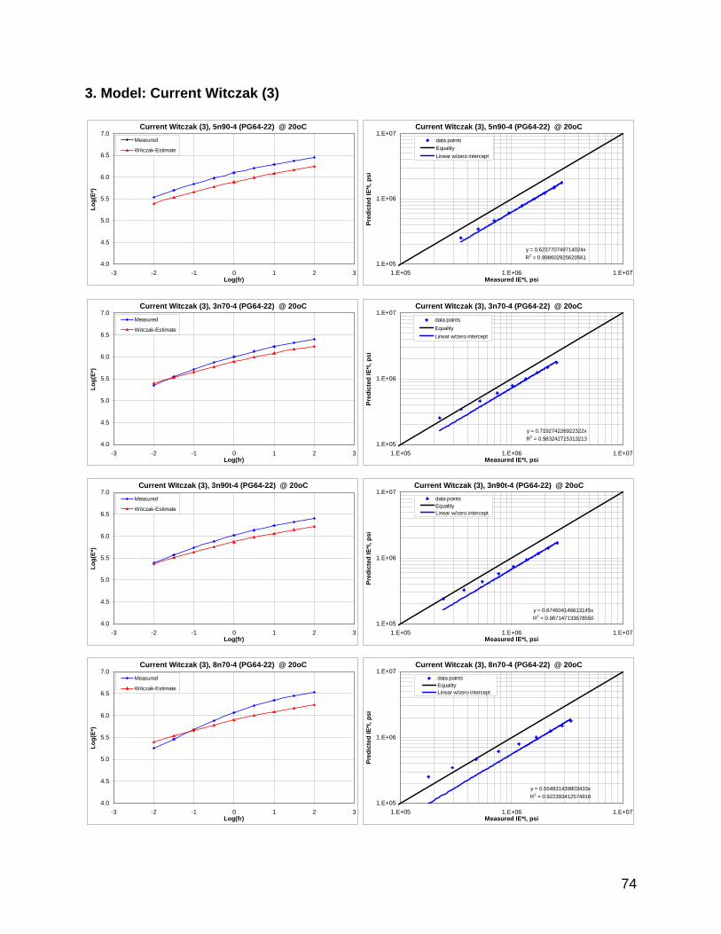
74
3. Model: Current Witczak (3)
Current Witczak (3), 5n90-4 (PG64-22) @ 20oC
4.0
4.5
5.0
5.5
6.0
6.5
7.0
-3 -2 -1 0 1 2 3Log(fr)
Log(
E*)
Measured
Witczak-Estimate
Current Witczak (3), 5n90-4 (PG64-22) @ 20oC
y = 0.623770749714024xR2 = 0.998602925620561
1.E+05
1.E+06
1.E+07
1.E+05 1.E+06 1.E+07Measured IE*I, psi
Pred
icte
d IE
*I, p
si
data pointsEqualityLinear w/zero intercept
Current Witczak (3), 3n70-4 (PG64-22) @ 20oC
4.0
4.5
5.0
5.5
6.0
6.5
7.0
-3 -2 -1 0 1 2 3Log(fr)
Log(
E*)
Measured
Witczak-Estimate
Current Witczak (3), 3n70-4 (PG64-22) @ 20oC
y = 0.719274226922322xR2 = 0.983242715313213
1.E+05
1.E+06
1.E+07
1.E+05 1.E+06 1.E+07Measured IE*I, psi
Pred
icte
d IE
*I, p
si
data pointsEqualityLinear w/zero intercept
Current Witczak (3), 3n90t-4 (PG64-22) @ 20oC
4.0
4.5
5.0
5.5
6.0
6.5
7.0
-3 -2 -1 0 1 2 3Log(fr)
Log(
E*)
Measured
Witczak-Estimate
Current Witczak (3), 3n90t-4 (PG64-22) @ 20oC
y = 0.674604146613145xR2 = 0.987147133678550
1.E+05
1.E+06
1.E+07
1.E+05 1.E+06 1.E+07Measured IE*I, psi
Pred
icte
d IE
*I, p
si
data pointsEqualityLinear w/zero intercept
Current Witczak (3), 8n70-4 (PG64-22) @ 20oC
4.0
4.5
5.0
5.5
6.0
6.5
7.0
-3 -2 -1 0 1 2 3Log(fr)
Log(
E*)
Measured
Witczak-Estimate
Current Witczak (3), 8n70-4 (PG64-22) @ 20oC
y = 0.554831439803433xR2 = 0.922393412574916
1.E+05
1.E+06
1.E+07
1.E+05 1.E+06 1.E+07Measured IE*I, psi
Pred
icte
d IE
*I, p
si
data pointsEqualityLinear w/zero intercept

75
4. Model: New Witczak
New Witczak (2), 3n90-4 (PG76-22) @ 20oC
4.0
4.5
5.0
5.5
6.0
6.5
7.0
-3 -2 -1 0 1 2 3Log(fr)
Log(
E*)
Measured
Witczak-Estimate
New Witczak (2), 3n90-4 (PG76-22) @ 20oC
y = 1.52342098711802xR2 = 0.91602636101094
1.E+05
1.E+06
1.E+07
1.E+05 1.E+06 1.E+07Measured IE*I, psi
Pred
icte
d IE
*I, p
si
data pointsEqualityLinear w/zero intercedpt
New Witczak (2), 5n90-4 (PG64-22) @ 20oC
4.0
4.5
5.0
5.5
6.0
6.5
7.0
-3 -2 -1 0 1 2 3Log(fr)
Log(
E*)
Measured
Witczak-Estimate
New Witczak (2), 5n90-4 (PG64-22) @ 20oC
y = 1.71169808006787xR2 = 0.97632279929626
1.E+05
1.E+06
1.E+07
1.E+05 1.E+06 1.E+07Measured IE*I, psi
Pred
icte
d IE
*I, p
si
data pointsEqualityLinear w/zero intercept
New Witczak (2), 5n105-4 (PG76-28) @ 20oC
4.0
4.5
5.0
5.5
6.0
6.5
7.0
-3 -2 -1 0 1 2 3Log(fr)
Log(
E*)
Measured
Witczak-Estimate
New Witczak (2), 5n105-4 (PG76-28) @ 20oC
y = 2.68370760506753xR2 = 0.98813977971917
1.E+05
1.E+06
1.E+07
1.E+05 1.E+06 1.E+07Measured IE*I, psi
Pred
icte
d IE
*I, p
si
data pointsEqualityLinear w/zero intercept
New Witczak (2), 1n80d-4 (PG76-28) @ 20oC
4.0
4.5
5.0
5.5
6.0
6.5
7.0
-3 -2 -1 0 1 2 3Log(fr)
Log(
E*)
Measured
Witczak-Estimate
New Witczak (2), 1n80d-4 (PG76-28) @ 20oC
y = 2.21433035564833xR2 = 0.98294197503951
1.E+05
1.E+06
1.E+07
1.E+05 1.E+06 1.E+07Measured IE*I, psi
Pred
icte
d IE
*I, p
si
data pointsEqualityLinear w/zero intercept
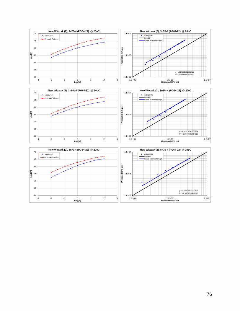
76
New Witczak (2), 3n70-4 (PG64-22) @ 20oC
4.0
4.5
5.0
5.5
6.0
6.5
7.0
-3 -2 -1 0 1 2 3Log(fr)
Log(
E*)
Measured
Witczak-Estimate
New Witczak (2), 3n70-4 (PG64-22) @ 20oC
y = 1.96757959508131xR2 = 0.99583310771111
1.E+05
1.E+06
1.E+07
1.E+05 1.E+06 1.E+07Measured IE*I, psi
Pred
icte
d IE
*I, p
si
data pointsEqualityLinear w/zero intercept
New Witczak (2), 3n90t-4 (PG64-22) @ 20oC
4.0
4.5
5.0
5.5
6.0
6.5
7.0
-3 -2 -1 0 1 2 3Log(fr)
Log(
E*)
Measured
Witczak-Estimate
New Witczak (2), 3n90t-4 (PG64-22) @ 20oC
y = 1.91927854177729xR2 = 0.99378082684629
1.E+05
1.E+06
1.E+07
1.E+05 1.E+06 1.E+07Measured IE*I, psi
Pred
icte
d IE
*I, p
si
data pointsEqualityLinear w/zero intercept
New Witczak (2), 8n70-4 (PG64-22) @ 20oC
4.0
4.5
5.0
5.5
6.0
6.5
7.0
-3 -2 -1 0 1 2 3Log(fr)
Log(
E*)
Measured
Witczak-Estimate
New Witczak (2), 8n70-4 (PG64-22) @ 20oC
y = 1.53553487513752xR2 = 0.99131890662367
1.E+05
1.E+06
1.E+07
1.E+05 1.E+06 1.E+07Measured IE*I, psi
Pred
cite
d IE
*I, p
si
data pointsEqualityLinear w/zero intercept
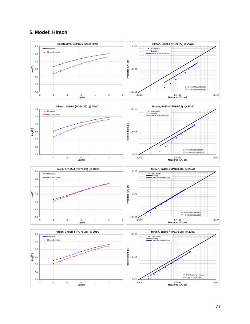
77
5. Model: Hirsch
Hirsch, 3n90-4 (PG76-22) @ 20oC
4.0
4.5
5.0
5.5
6.0
6.5
7.0
-3 -2 -1 0 1 2 3Log(fr)
Log(
E*)
Measured
Hirsch-Estimate
Hirsch, 5n90-4 (PG64-22) @ 20oC
4.0
4.5
5.0
5.5
6.0
6.5
7.0
-3 -2 -1 0 1 2 3Log(fr)
Log(
E*)
Measured
Hirsch-Estimate
Hirsch, 5n105-4 (PG76-28) @ 20oC
4.0
4.5
5.0
5.5
6.0
6.5
7.0
-3 -2 -1 0 1 2 3Log(fr)
Log(
E*)
Measured
Hirsch-Estimate
Hirsch, 1n80d-4 (PG76-28) @ 20oC
4.0
4.5
5.0
5.5
6.0
6.5
7.0
-3 -2 -1 0 1 2 3Log(fr)
Log(
E*)
Measured
Hirsch-Estimate
Hirsch, 3n90-4 (PG76-22) @ 20oC
y = 0.563182511925906xR2 = 0.942898698882482
1.E+05
1.E+06
1.E+07
1.E+05 1.E+06 1.E+07Measured IE*I, psi
Pred
icte
d IE
*I, p
si
data pointsEqualityLinear w/zero intercept
Hirsch, 5n90-4 (PG64-22) @ 20oC
y = 0.686231315514568xR2 = 0.980467003766921
1.E+05
1.E+06
1.E+07
1.E+05 1.E+06 1.E+07Measured IE*I, psi
Pred
icte
d IE
*I, p
si
data pointsEqualityLinear w/zero intercept
Hirsch, 5n105-4 (PG76-28) @ 20oC
y = 1.03039091690398xR2 = 0.99289468156304
1.E+05
1.E+06
1.E+07
1.E+05 1.E+06 1.E+07Measured IE*I, psi
Pred
icte
d IE
*I, p
si
data pointsEqualityLinear w/zero intercept
Hirsch, 1n80d-4 (PG76-28) @ 20oC
y = 0.767915731244611xR2 = 0.994833586105611
1.E+05
1.E+06
1.E+07
1.E+05 1.E+06 1.E+07Measured IE*I, psi
Pred
icte
d IE
*I, p
si
data pointsEqualityLinear w/zero intercept

78
Hirsch, 3n70-4 (PG64-22) @ 20oC
4.0
4.5
5.0
5.5
6.0
6.5
7.0
-3 -2 -1 0 1 2 3Log(fr)
Log(
E*)
Measured
Hirsch-Estimate
Hirsch, 3n90t-4 (PG64-22) @ 20oC
4.0
4.5
5.0
5.5
6.0
6.5
7.0
-3 -2 -1 0 1 2 3Log(fr)
Log(
E*)
Measured
Hirsch-Estimate
Hirsch, 8n70-4 (PG64-22) @ 20oC
4.0
4.5
5.0
5.5
6.0
6.5
7.0
-3 -2 -1 0 1 2 3Log(fr)
Log(
E*)
Measured
Hirsch-Estimate
Hirsch, 3n70-4 (PG64-22) @ 20oC
y = 0.794073352529366xR2 = 0.996199017740505
1.E+05
1.E+06
1.E+07
1.E+05 1.E+06 1.E+07Measured IE*I, psi
Pred
icte
d IE
*I, p
si
data pointsEqualityLinear w/zero intercept
Hirsch, 3n90t-4 (PG64-22) @ 20oC
y = 0.784598189860344xR2 = 0.994458166929060
1.E+05
1.E+06
1.E+07
1.E+05 1.E+06 1.E+07Measured IE*I, psi
Pred
cite
d IE
*I, p
si
data pointsEqualityLinear w/zero intercept
Hirsch, 8n70-4 (PG64-22) @ 20oC
y = 0.633977407109956xR2 = 0.990042730245701
1.E+05
1.E+06
1.E+07
1.E+05 1.E+06 1.E+07Measured IE*I, psi
Pred
cite
d IE
*I, p
si
data pointsEqualityLinear w/zero intercept

79
APPENDIX D

80
1. Model: Current Witczak (1)
Current Witczak (1), 5n70-4 (PG64-22) @ 20oC
4.0
4.5
5.0
5.5
6.0
6.5
7.0
-3 -2 -1 0 1 2 3Log(fr)
Log(
E*)
Measured
Witczak-Estimate
Current Witczak (1), 5n70-4 (PG64-22) @ 20oC
y = 0.577608682520614xR2 = 0.9805556188330061.E+05
1.E+06
1.E+07
1.E+05 1.E+06 1.E+07Measured IE*I, psi
Pred
icte
d IE
*I, p
si
data pointsEqualityLinear w/zero intercept
Current Witczak (1), 6n50-4 (PG64-22) @ 20oC
4.0
4.5
5.0
5.5
6.0
6.5
7.0
-3 -2 -1 0 1 2 3Log(fr)
Log(
E*)
Measured
Witczak-Estimate
Current Witczak (1), 6n50-4 (PG64-22) @ 20oC
y = 0.565339310873371xR2 = 0.978398915269107
1.E+05
1.E+06
1.E+07
1.E+05 1.E+06 1.E+07Mesured IE*I, psi
Pred
icte
d IE
*I, p
si
data pointsEqualityLinear w/zero intercept
Current Witczak (1), 9n90-4 (PG64-22) @ 20oC
4.0
4.5
5.0
5.5
6.0
6.5
7.0
-3 -2 -1 0 1 2 3Log(fr)
Log(
E*)
Measured
Witczak-Estimate
Current Witczak (1), 9n90-4 (PG64-22) @ 20oC
y = 0.4404347316107xR2 = 0.99636315380091.E+05
1.E+06
1.E+07
1.E+05 1.E+06 1.E+07Measured IE*I, psi
Pred
icte
d IE
*I, p
si
data pointsEqualityLinear w/zero intercept
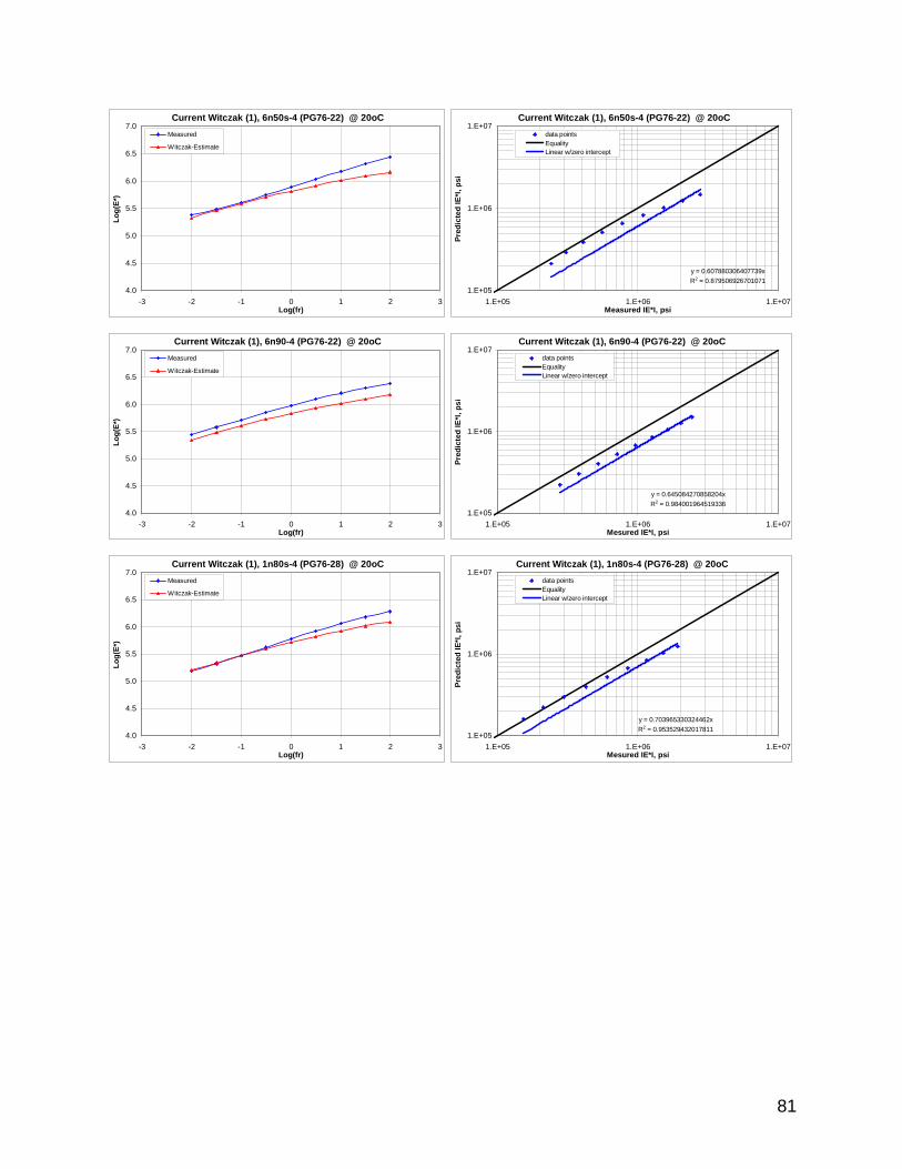
81
Current Witczak (1), 6n50s-4 (PG76-22) @ 20oC
4.0
4.5
5.0
5.5
6.0
6.5
7.0
-3 -2 -1 0 1 2 3Log(fr)
Log(
E*)
Measured
Witczak-Estimate
Current Witczak (1), 6n50s-4 (PG76-22) @ 20oC
y = 0.607880306407739xR2 = 0.879506926701071
1.E+05
1.E+06
1.E+07
1.E+05 1.E+06 1.E+07Measured IE*I, psi
Pred
icte
d IE
*I, p
si
data pointsEqualityLinear w/zero intercept
Current Witczak (1), 6n90-4 (PG76-22) @ 20oC
4.0
4.5
5.0
5.5
6.0
6.5
7.0
-3 -2 -1 0 1 2 3Log(fr)
Log(
E*)
Measured
Witczak-Estimate
Current Witczak (1), 6n90-4 (PG76-22) @ 20oC
y = 0.645084270858204xR2 = 0.984001964519336
1.E+05
1.E+06
1.E+07
1.E+05 1.E+06 1.E+07Mesured IE*I, psi
Pred
icte
d IE
*I, p
si
data pointsEqualityLinear w/zero intercept
Current Witczak (1), 1n80s-4 (PG76-28) @ 20oC
4.0
4.5
5.0
5.5
6.0
6.5
7.0
-3 -2 -1 0 1 2 3Log(fr)
Log(
E*)
Measured
Witczak-Estimate
Current Witczak (1), 1n80s-4 (PG76-28) @ 20oC
y = 0.703965330324462xR2 = 0.953529432017811
1.E+05
1.E+06
1.E+07
1.E+05 1.E+06 1.E+07Mesured IE*I, psi
Pred
icte
d IE
*I, p
si
data pointsEqualityLinear w/zero intercept

82
Current Witczak (1), 1n105-4 (PG70-22) @ 20oC
4.0
4.5
5.0
5.5
6.0
6.5
7.0
-3 -2 -1 0 1 2 3Log(fr)
Log(
E*)
Measured
Witczak-Estimate
Current Witczak (1), 1n105-4 (PG70-22) @ 20oC
y = 0.508610505569145xR2 = 0.997148422132926
1.E+05
1.E+06
1.E+07
1.E+05 1.E+06 1.E+07Mesured IE*I, psi
Pred
icte
d IE
*I, p
si
data pointsEqualityLinear w/zero intercept
Current Witczak (1), 2n90-4 (PG70-22) @ 20oC
4.0
4.5
5.0
5.5
6.0
6.5
7.0
-3 -2 -1 0 1 2 3Log(fr)
Log(
E*)
Measured
Witczak-Estimate
Current Witczak (1), 2n90-4 (PG70-22) @ 20oC
y = 0.512688918335139xR2 = 0.996802664389056
1.E+05
1.E+06
1.E+07
1.E+05 1.E+06 1.E+07Mesured IE*I, psi
Pred
icte
d IE
*I, p
si
data pointsEqualityLinear w/zero intercept
Current Witczak (1), 8n105-4 (PG70-22) @ 20oC
4.0
4.5
5.0
5.5
6.0
6.5
7.0
-3 -2 -1 0 1 2 3Log(fr)
Log(
E*)
Measured
Witczak-Estimate
Current Witczak (1), 8n105-4 (PG70-22) @ 20oC
y = 0.560565657235306xR2 = 0.997269403639920
1.E+05
1.E+06
1.E+07
1.E+05 1.E+06 1.E+07Mesured IE*I, psi
Pred
icte
d IE
*I, p
si
data pointsEqualityLinear w/zero intercept

83
2. Model: Hirsch
Hirsch, 5n70-4 (PG64-22) @ 20oC
4.0
4.5
5.0
5.5
6.0
6.5
7.0
-3 -2 -1 0 1 2 3Log(fr), Hz
Log(
E*),
psi
Measured
Hirsch-Estimate
Hirsch, 6n50-4 (PG64-22) @ 20oC
4.0
4.5
5.0
5.5
6.0
6.5
7.0
-3 -2 -1 0 1 2 3Log(fr)
Log(
E*)
Measured
Hirsch-Estimate
Hirsch, 9n90-4 (PG64-22) @ 20oC
4.0
4.5
5.0
5.5
6.0
6.5
7.0
-3 -2 -1 0 1 2 3Log(fr)
Log(
E*)
Measured
Hirsch-Estimate
Hirsch, 5n70-4 (PG64-22) @ 20oC
y = 0.887746521904192xR2 = 0.998914989320803
1.E+05
1.E+06
1.E+07
1.E+05 1.E+06 1.E+07Measured IE*I, psi
Pred
icte
d IE
*I, p
si
data points
Equality
Linear w/zero intercept
Hirsch, 6n50-4 (PG64-22) @ 20oC
y = 0.786369377696736xR2 = 0.997073281559625
1.E+05
1.E+06
1.E+07
1.E+05 1.E+06 1.E+07Measured IE*I, psi
Pred
icte
d IE
*I, p
si
data pointsEqualityLinear w/zero intercept
Hirsch, 9n90-4 (PG64-22) @ 20oC
y = 0.659506087818202xR2 = 0.989039533208399
1.E+05
1.E+06
1.E+07
1.E+05 1.E+06 1.E+07Measured IE*I, psi
Pred
icte
d IE
*I, p
si
data pointsEqualityLinear w/zero intercept
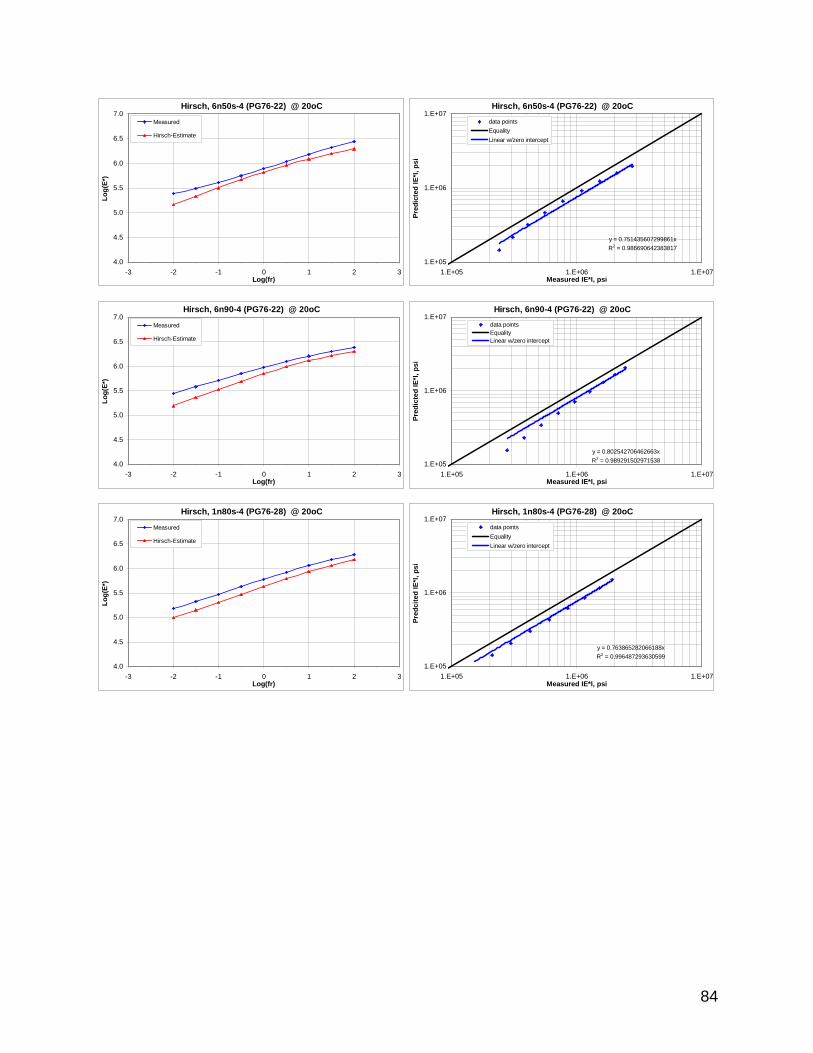
84
Hirsch, 6n50s-4 (PG76-22) @ 20oC
4.0
4.5
5.0
5.5
6.0
6.5
7.0
-3 -2 -1 0 1 2 3Log(fr)
Log(
E*)
Measured
Hirsch-Estimate
Hirsch, 6n90-4 (PG76-22) @ 20oC
4.0
4.5
5.0
5.5
6.0
6.5
7.0
-3 -2 -1 0 1 2 3Log(fr)
Log(
E*)
Measured
Hirsch-Estimate
Hirsch, 1n80s-4 (PG76-28) @ 20oC
4.0
4.5
5.0
5.5
6.0
6.5
7.0
-3 -2 -1 0 1 2 3Log(fr)
Log(
E*)
Measured
Hirsch-Estimate
Hirsch, 6n50s-4 (PG76-22) @ 20oC
y = 0.751435607299861xR2 = 0.986690642383817
1.E+05
1.E+06
1.E+07
1.E+05 1.E+06 1.E+07Measured IE*I, psi
Pred
icte
d IE
*I, p
si
data pointsEqualityLinear w/zero intercept
Hirsch, 6n90-4 (PG76-22) @ 20oC
y = 0.802542706462663xR2 = 0.9892915029715381.E+05
1.E+06
1.E+07
1.E+05 1.E+06 1.E+07Measured IE*I, psi
Pred
icte
d IE
*I, p
si
data pointsEqualityLinear w/zero intercept
Hirsch, 1n80s-4 (PG76-28) @ 20oC
y = 0.763865282066188xR2 = 0.996487293630599
1.E+05
1.E+06
1.E+07
1.E+05 1.E+06 1.E+07Measured IE*I, psi
Pred
cite
d IE
*I, p
si
data pointsEqualityLinear w/zero intercept

85
Hirsch, 1n105-4 (PG70-22) @ 20oC
4.0
4.5
5.0
5.5
6.0
6.5
7.0
-3 -2 -1 0 1 2 3Log(fr)
Log(
E*)
Measured
Hirsch-Estimate
Hirsch, 1n105-4 (PG70-22) @ 20oC
y = 0.626304392728516xR2 = 0.988413949150349
1.E+05
1.E+06
1.E+07
1.E+05 1.E+06 1.E+07Measured IE*I, psi
Pred
cite
d IE
*I, p
si
data pointsEqualityLinear w/zero intercept
Hirsch, 2n90-4 (PG70-22) @ 20oC
4.0
4.5
5.0
5.5
6.0
6.5
7.0
-3 -2 -1 0 1 2 3Log(fr)
Log(
E*)
Measured
Hirsch-Estimate
Hirsch, 2n90-4 (PG70-22) @ 20oC
y = 0.656180269408445xR2 = 0.989641203491579
1.E+05
1.E+06
1.E+07
1.E+05 1.E+06 1.E+07Measured IE*I, psi
Pred
cite
d IE
*I, p
si
data pointsEqualityLinear w/zero intercept
Hirsch, 8n105-4 (PG70-22) @ 20oC
4.0
4.5
5.0
5.5
6.0
6.5
7.0
-3 -2 -1 0 1 2 3Log(fr)
Log(
E*)
Measured
Hirsch-Estimate
Hirsch, 8n105-4 (PG70-22) @ 20oC
y = 0.666745542239858xR2 = 0.981194539041125
1.E+05
1.E+06
1.E+07
1.E+05 1.E+06 1.E+07Measured IE*I, psi
Pred
cite
d IE
*I, p
si
data pointsEqualityLinear w/zero intercept

86
APPENDIX E

87
1. Mixture: 1111
Mix Temp., oC f, Hz log(f ) E*, psi log(E*)20 25 1.39794 2,097,520 6.3217 log(E*) = δ+[α/(1+eβ−γ [log(fr)+log(aT)]]20 10 1 2,206,646 6.3437 E*, psi; fr, Hz; T,oC (T fix, fr variable)20 1 0 1,344,530 6.1286
20 0.1 -1 679,203 5.8320 log(E*) = δ+[α/(1+eβ−γ [log(fr)+log(aT)]]20 0.01 -2 336,466 5.5269 E*, psi; fr, Hz; T,oC (T variable, fr fix)4 25 1.39794 3,494,612 6.54344 10 1 4,043,934 6.6068 α β γ δ4 1 0 3,266,187 6.5140 1.602024 -0.78172 0.755401 5.0111664 0.1 -1 2,374,065 6.37554 0.01 -2 1,489,766 6.1731
-10 25 1.39794 2,991,874 6.4759-10 10 1 4,638,028 6.6663-10 1 0 4,115,942 6.6145-10 0.1 -1 3,534,645 6.5483-10 0.01 -2 2,817,165 6.4498
1111
E* Master Curve Equation
E* Isochronal Equation
1111 (MC) @ ToC
5.00
5.25
5.50
5.75
6.00
6.25
6.50
6.75
7.00
-7 -6 -5 -4 -3 -2 -1 0 1 2 3 4 5 6 7 8Log(fr)
Log(
E*)
-10oC4oC20oCMC@-10oCMC@4oCMC@20oCMC@30oC
1111, Shift Factors (Tm=20oC)
y = -0.00107703301846515x2 - 0.11773350521881700x + 2.78548331176239000
R2 = 0.999999999999999000
1
2
3
4
5
-15 -5 5 15 25T, oC
Log(
aT)
Sigmoidal(solver)
Poly.(Si id l( l ))
1111, Lab Data
4.0
4.5
5.0
5.5
6.0
6.5
7.0
-3 -2 -1 0 1 2 3 4 5 6 7Log(fr)
Log(
E*)
-10oC
4oC
20oC
1111 (Isochronal) @ f Hz
5.80
5.90
6.00
6.10
6.20
6.30
6.40
6.50
6.60
6.70
-10 -5 0 5 10 15 20 25 30Temperature, oC
Log(
E*)
5Hz
10Hz
20Hz

88
2. Mixture: 1112
Mix Temp., oC f, Hz log(f ) E*, psi log(E*)20 25 1.39794 2,203,313 6.3431 log(E*) = δ+[α/(1+eβ−γ [log(fr)+log(aT)]]20 10 1 2,030,642 6.3076 E*, psi; fr, Hz; T,oC (T fix, fr variable)20 1 0 1,299,947 6.1139
20 0.1 -1 664,439 5.8225 log(E*) = δ+[α/(1+eβ−γ [log(fr)+log(aT)]]20 0.01 -2 305,866 5.4855 E*, psi; fr, Hz; T,oC (T variable, fr fix)4 25 1.39794 3,241,872 6.51084 10 1 4,334,020 6.6369 α β γ δ4 1 0 3,498,720 6.5439 1.739043 -0.64468 0.722148 4.9603474 0.1 -1 2,593,008 6.41384 0.01 -2 1578163 6.1982
-10 25 1.39794 3474792 6.5409-10 10 1 5014973 6.7003-10 1 0 6315779 6.8004-10 0.1 -1 5517923 6.7418-10 0.01 -2 4470674 6.6504
1112
E* Master Curve Equation
E* Isochronal Equation
1112 (MC) @ ToC
5.00
5.25
5.50
5.75
6.00
6.25
6.50
6.75
7.00
-7 -6 -5 -4 -3 -2 -1 0 1 2 3 4 5 6 7 8Log(fr)
Log(
E*)
-10oC4oC20oCMC@-10oCMC@4oCMC@20oCMC@30oC
1112, Shift Factors (Tm=20oC)
y = 0.000749931461802772x2 - 0.162699809987389000x + 2.954023615026680000
R2 = 1.0000000000000000000
1
2
3
4
5
-15 -10 -5 0 5 10 15 20 25T, oC
Log(
aT)
Sigmoidal(solver)Poly. (Sigmoidal(solver))
1112, Lab Data
5.00
5.25
5.50
5.75
6.00
6.25
6.50
6.75
7.00
-3 -2 -1 0 1 2 3 4 5 6 7Log(fr)
Log(
E*)
-10oC
4oC
20oC
1112 (Isochronal) @ f Hz
5.80
5.90
6.00
6.10
6.20
6.30
6.40
6.50
6.60
6.70
-10 -5 0 5 10 15 20 25 30Temperature, oC
Log(
E*)
5Hz
10Hz
20Hz

89
3. Mixture: 1113
Mix Temp., oC f, Hz log(f ) E*, psi log(E*)20 25 1.39794 1,824,443 6.2611 log(E*) = δ+[α/(1+eβ−γ [log(fr)+log(aT)]]20 10 1 2,140,825 6.3306 E*, psi; fr, Hz; T,oC (T fix, fr variable)20 1 0 1,371,719 6.1373
20 0.1 -1 670,687 5.8265 log(E*) = δ+[α/(1+eβ−γ [log(fr)+log(aT)]]20 0.01 -2 312,614 5.4950 E*, psi; fr, Hz; T,oC (T variable, fr fix)4 25 1.39794 2,434,779 6.38654 10 1 2,920,849 6.4655 α β γ δ4 1 0 2,183,260 6.3391 4.1 -1.75947 0.429632 2.5969684 0.1 -1 1,517,346 6.18114 0.01 -2 917,906 5.9628
-10 25 1.39794 3,881,141 6.5890-10 10 1 4,998,322 6.6988-10 1 0 4,443,724 6.6477-10 0.1 -1 3,823,416 6.5825-10 0.01 -2 3,109,085 6.4926
1113
E* Master Curve Equation
E* Isochronal Equation
1113 (MC) @ ToC
5.00
5.25
5.50
5.75
6.00
6.25
6.50
6.75
7.00
-7 -6 -5 -4 -3 -2 -1 0 1 2 3 4 5 6 7 8Log(fr)
Log(
E*)
-10oC4oC20oCMC@-10oCMC@4oCMC@20oCMC@30oC
1113, Shift Factors (Tm=20oC)
y = 0.139778130979674xR2 = 0.914827558422635
0
1
2
3
4
5
-5 0 5 10 15 20 25 30 35Tm-T, oC
Log(
aT)
Sigmoidal(solver)Linear (Sigmoidal(solver))
1113, Lab Data
5.0
5.3
5.5
5.8
6.0
6.3
6.5
6.8
7.0
-3 -2 -1 0 1 2 3 4 5 6 7Log(fr)
Log(
E*)
-10oC
4oC
20oC
1113 (Isochronal) @ f Hz
5.80
5.90
6.00
6.10
6.20
6.30
6.40
6.50
6.60
6.70
-10 -5 0 5 10 15 20 25 30Temperature, oC
Log(
E*)
5Hz
10Hz
20Hz

90
4. Mixture: 1114
Mix Temp., oC f, Hz log(f ) E*, psi log(E*)20 25 1.39794 2,041,097 6.3099 log(E*) = δ+[α/(1+eβ−γ [log(fr)+log(aT)]]20 10 1 2,128,214 6.3280 E*, psi; fr, Hz; T,oC (T fix, fr variable)20 1 0 1,316,190 6.1193
20 0.1 -1 625,151 5.7960 log(E*) = δ+[α/(1+eβ−γ [log(fr)+log(aT)]]20 0.01 -2 272,153 5.4348 E*, psi; fr, Hz; T,oC (T variable, fr fix)4 25 1.39794 2,803,645 6.44774 10 1 4,277,077 6.6311 α β γ δ4 1 0 3,996,847 6.6017 2.12725 -1.07539 0.668007 4.5131824 0.1 -1 3,025,883 6.48094 0.01 -2 2,233,748 6.3490
-10 25 1.39794 3,467,708 6.5400-10 10 1 5,049,423 6.7032-10 1 0 4,748,463 6.6766-10 0.1 -1 4,225,790 6.6259-10 0.01 -2 3,534,265 6.5483
E* Master Curve Equation
E* Isochronal Equation
1114
1114 (MC) @ ToC
5.00
5.25
5.50
5.75
6.00
6.25
6.50
6.75
7.00
-7 -6 -5 -4 -3 -2 -1 0 1 2 3 4 5 6 7 8Log(fr)
Log(
E*)
-10oC4oC20oCMC@-10oCMC@4oCMC@20oCMC@30oC
1114, Shift Factors (Tm=20oC)
y = 0.164415389484397xR2 = 0.969557845853866
0
1
2
3
4
5
-5 0 5 10 15 20 25 30 35Tm-T, oC
Log(
aT)
Sigmoidal(solver)Linear (Sigmoidal(solver))
1114, Lab Data
5.00
5.25
5.50
5.75
6.00
6.25
6.50
6.75
7.00
-3 -2 -1 0 1 2 3 4 5 6 7Log(fr)
Log(
E*)
-10oC
4oC
20oC
1114 (Isochronal) @ f Hz
5.80
5.90
6.00
6.10
6.20
6.30
6.40
6.50
6.60
6.70
-10 -5 0 5 10 15 20 25 30Temperature, oC
Log(
E*)
5Hz
10Hz
20Hz

91
5. Mixture: 3809
Mix Temp., oC f, Hz log(f ) E*, psi log(E*)20 25 1.39794 2,612,918 6.4171 log(E*) = δ+[α/(1+eβ−γ [log(fr)+log(aT)]]20 10 1 1,909,999 6.2810 E*, psi; fr, Hz; T,oC (T fix, fr variable)20 1 0 1,176,645 6.0706
20 0.1 -1 553,203 5.7429 log(E*) = δ+[α/(1+eβ−γ [log(fr)+log(aT)]]20 0.01 -2 292,628 5.4663 E*, psi; fr, Hz; T,oC (T variable, fr fix)4 25 1.39794 2,875,231 6.45874 10 1 3,817,938 6.5818 α β γ δ4 1 0 2,662,702 6.4253 1.438825 -0.53217 0.904103 5.1545264 0.1 -1 1,659,677 6.22004 0.01 -2 880,407 5.9447
-10 25 1.39794 3,219,439 6.5078-10 10 1 4,505,126 6.6537-10 1 0 3,643,987 6.5616-10 0.1 -1 2,933,225 6.4673-10 0.01 -2 2,134,690 6.3293
3809
E* Master Curve Equation
E* Isochronal Equation
3809 (MC) @ ToC
5.00
5.25
5.50
5.75
6.00
6.25
6.50
6.75
7.00
-7 -6 -5 -4 -3 -2 -1 0 1 2 3 4 5 6 7 8Log(fr)
Log(
E*)
-10oC4oC20oCMC@-10oCMC@4oCMC@20oCMC@30oC
3809, Shift Factors (Tm=20oC)
y = 0.000132147742967175x2 - 0.104058315092609000x + 2.028307204665310000
R2 = 0.9999999999999990000
1
2
3
4
-15 -10 -5 0 5 10 15 20 25T, oC
Log(
aT)
Sigmoidal(solver)
Poly. (Sigmoidal(solver))
3809, Lab Data
5.00
5.25
5.50
5.75
6.00
6.25
6.50
6.75
7.00
-3 -2 -1 0 1 2 3 4 5 6 7Log(fr)
Log(
E*)
-10oC
4oC
20oC
3809 (Isochronal) @ f Hz
5.80
5.90
6.00
6.10
6.20
6.30
6.40
6.50
6.60
6.70
-10 -5 0 5 10 15 20 25 30Temperature, oC
Log(
E*)
5Hz
10Hz
20Hz