I

THESIS FOR THE DEGREE OF DOCTOR OF PHILOSOPHY

Citrus Waste Biorefinery: Process Development, Simulation and

Economic Analysis

MOHAMMAD POUR BAFRANI

Department of Chemical and Biological Engineering

CHALMERS UNIVERSITY OF TECHNOLOGY

Göteborg, Sweden 2010

II

Citrus Waste Biorefinery: Process Development, Simulation and Economic Analysis

Mohammad Pour Bafrani

ISBN: 978-91-7385-388-0

Copyright © Mohammad Pour Bafrani, 2010

Doktorsavhandlingar vid Chalmers Tekniska Högskola

Ny serie nr: 3069

ISSN: 0346-718X

Published and distributed by:

Chemical Reaction Engineering

Chemical and Biological Engineering

Chalmers University of Technology

SE-412 96 Göteborg

Sweden

Telephone +46(0)31-772 1000

www.chalmers.se

Cover image: A picture of the production of ethanol, methane and limonene from citrus

wastes

Printed by Chalmers Reproservice

Göteborg, Sweden, 2010

III

Citrus Waste Biorefinery: Process Development, Simulation and Economic Analysis

Mohammad Pour Bafrani

Chemical Reaction Engineering

Department of Chemical and Biological Engineering

Chalmers University of Technology, SE-412 96 Göteborg, Sweden

Abstract ---------------------------------------------------------------------------------------------------------------

The production of ethanol and other sustainable products including methane, limonene and

pectin from citrus wastes (CWs) was studied in the present thesis. In the first part of the work,

the CWs were hydrolyzed using enzymes – pectinase, cellulase and β-glucosidase – and the

hydrolyzate was fermented using encapsulated yeasts in the presence of the inhibitor

compound ‘limonene’. However, the application of encapsulated cells may be hampered by

the high price of encapsulation, enzymes and the low stability of capsules’ membrane at high

shear stresses.

Therefore, a process based on dilute-acid hydrolysis of CWs was developed. The limonene of

the CWs was effectively removed through flashing of the hydrolyzate into an expansion tank.

The sugars present in the hydrolyzate were converted to ethanol using a flocculating yeast

strain. Then ethanol was distilled and the stillage and the remaining solid materials of the

hydrolyzed CWs were anaerobically digested to obtain methane. The soluble pectin content of

hydrolyzate can be precipitated using the produced ethanol. One ton of CWs with 20% dry

weight resulted in 39.64 l ethanol, 45 m3 methane, 8.9 l limonene, and 38.8 kg pectin. The

feasibility of the process depends on the transportation cost and the capacity of CW. For

example, the total cost of ethanol with a capacity of 100,000 tons CW/year was 0.91 USD/L,

assuming 10 USD/ton handling and transportation cost of CW to the plant. Changing the plant

capacity from 25,000 to 400,000 tons CW per year results in reducing ethanol costs from 2.55

to 0.46 USD/L in an economically feasible process.

Since this process employs a flocculating yeast strain, the major concern in design of the

bioreactor is the sedimentation of yeast flocs. The size of flocs is a function of sugar

concentration, time and flow. A CFD model of bioreactor was developed to predict the

sedimentation of flocs and the effect of flow on distribution of flocs. The CFD model

predicted that the flocs sediment when they are larger than 180 micrometer. The developed

CFD model can be used in design and scale-up of the bioreactor.

For the plants with low CW capacity, a steam explosion process was employed to eliminate

limonene and the treated CW was used in a digestion plant to produce methane. The required

cost of this pretreatment was about 0.90 million dollars for 10,000 tons/year of CWs.

Keywords: Citrus wastes, ethanol, methane, pectin, limonene, encapsulated yeast, economic

analysis, process simulation, computational fluid dynamic simulation.

IV

LIST OF PUBLICATIONS

This thesis is based on the work contained in the following papers:

I Mohammad Pourbafrani, Farid Talebnia, Claes Niklasson, Mohammad J. Taherzadeh,

Protective Effect of Encapsulation in Fermentation of Limonene-contained Media and Orange

Peel Hydrolyzate, International Journal of Molecular Science, 2007, 8(8), 777-787.

II Farid Talebnia, Mohammad Pourbafrani, Magnus Lundin, Mohammad J. Taherzadeh,

Optimization Study of Citrus Wastes Saccharification by Dilute-Acid Hydrolysis,

Bioresources, 2008, 3(1), 108-122.

III Mohammad Pourbafrani, Gergoly Forgács, Ilona Sárvári Horváth, Claes Niklasson,

Mohammad J. Taherzadeh, Production of biofuels, limonene and pectin from citrus wastes,

Bioresource Technology, 2010, 101(11), 4246-4250.

IV Mehdi Lohrasbi, Mohammad Pourbafrani, Claes Niklasson, Mohammad J. Taherzadeh, Process design and economic analysis of a citrus waste biorefinery with biofuels and

limonene as products. Accepted for publication in Bioresource Technology, 2010.

V Mohammad Pourbafrani, Bengt Andersson, Claes Niklasson, Mohammad J.

Taherzadeh, Quantification of yeast flocculation and computational fluid dynamic simulation

of the flocculation process. Submitted to International Journal of Chemical Reactor

Engineering.

Part of this work is under progress for patenting and the patent application number is

0901415-0.

Contribution Report:

Paper I: Responsible for the idea, experimental work, and writing some parts of the paper.

Paper II: Responsible for experimental design, experimental work and writing some parts of

the paper.

Paper III: Responsible for the idea, experimental design, experimental work and all writing.

Paper IV: Responsible for the idea, simulation, supervising the work, some parts of

economic calculations and writing some parts of the paper.

Paper V: Responsible for the idea, experimental work, simulation and all writing.

V

Content

1.Introduction 1

1.1.Scope 2

2. Experiments

3

2.1. Feedstock and Enzymes 3

2.2. Mechanical Pretreatment and Enzymatic Hydrolysis 3

2.3. Dilute Acid Hydrolysis 4

2.4. Pectin Recovery 5

2.5. Medium 5

2.6. Encapsulation 5

2.7. Fermentation 6

2.8. Average Diameter of Yeast Flocs 7

2.9. Anaerobic Digestion 8

2.10. Analyses

8

3. Conceptual Design

11

3.1. Process Block Flow Diagram 11

3.2. Process Simulation Using Aspen Plus 12

3.2.1. Components 12

3.2.2. Reactions 12

3.2.3. Thermodynamic Model 13

3.2.4. Unit Operations 13

3.3. Process Design 14

3.3.1. Hydrolysis and Limonene Recovery 14

3.3.2. Fermentation 14

3.3.3. Distillation 15

3.3.4. Anaerobic digestion 16

3.3.5. Wastewater treatment 16

3.4. Economic Analysis 16

3.4.1. Capital Cost Estimation Using Aspen Icarus Process Evaluator 16

3.4.2. Fixed Capital Investment 17

3.4.3. Cost of Manufacturing 17

3.4.4. Ethanol Selling Price 18

3.5. Sensitivity Analysis 18

4. Computational Fluid Dynamic Simulation

19

4.1. Flow Modeling in CFD 19

4.1.1. Single Phase Flow 19

4.1.1.1. Turbulence Modeling 20

4.1.1.2. Realizable k Turbulence model 21

4.1.1.3. Reynolds Stress Turbulence model 22

VI

4.1.2. Multiphase Simulation 22

4.1.2.1. Mixture Model 22

4.2. Flow Simulation 23

4.3. Simulation of Yeast Flocs Distribution 23

5. Result and Discussion

25

5.1. Enzymatic Hydrolysis 25

5.2. Process Based on Dilute Acid Hydrolysis 27

5.2.1. Dilute Acid Hydrolysis at Low Temperature 27

5.2.2. Dilute Acid Hydrolysis at High Temperature 28

5.2.3. Fermentation 29

5.2.4. Pectin Recovery 29

5.2.5. Methane production 30

5.2.6. Overall Process 30

5.3. Process Detail for Large Scale Utilizing of Citrus Wastes 31

5.3.1. Material Balance 31

5.3.2. Energy Analysis 31

5.3.3. Fixed Capital Cost (FCI) 32

5.3.4. Cost of Manufacturing 33

5.3.5. Ethanol Production Cost 33

5.3.6. Comparison with Previous Processes 35

5.4. Process Detail for Low Scale Utilizing of Citrus Wastes 35

5.5. Computational Fluid Dynamic Simulation Results 37

5.5.1. Flow Simulation 37

5.5.1.1. Turbulence Intensity 37

5.5.1.2. Turbulence Dissipation Rate 38

5.5.1.3.Velocity Contours 38

5.5.2. Simulation of Yeast Flocs Distribution 39

6. Conclusion

7. Future Work

41

42

Nomenclature 43

Acknowledgement 46

References 47

1

1. Introduction

Ethanol is nowadays an important factor in the fuel market due to its renewable sources

and the concerns about global warming and energy resources. Starch- and sugar-based

materials such as sugarcane and corn are considered as a first-generation source for fuel

ethanol. The availability of agricultural land for non-food crops and the limited market for

animal feed restricts the amount of ethanol that can be produced from starch-based materials

(Perlack et al., 2006). Ethanol production from lignocellulosic raw materials such as

agricultural wastes and wood residues reduces the potential conflict between land use for food

production and energy feedstock production (Galbe et al., 2007).

Citrus wastes (CWs) have been considered as a feedstock for ethanol production since 1992

(Grohmann and Baldwin, 1992). The estimated worldwide production of CWs is 15 million

tons per year (Marin et al., 2007). Currently, parts of the CWs are dried and marketed as low-

protein cattle feed called “citrus pulp pellets” and the rest are disposed in landfills,

constituting severe economic and environmental problems (Tripodo et al., 2004).

The main obstacle in production of ethanol from CWs is the presence of d-limonene (C10H16;

1-methyl-4-prop-1-en-2-yl-cyclohexene) in CWs. Limonene is extremely toxic for

Saccharomyces cerevisiae (Stewart et al., 2005) and it can be a strong inhibitor at even low

concentration or a lethal component at high concentration. Furthermore, carbohydrate

polymers of CWs should be depolymerized to their monomer sugars before fermentation. The

breakdown of carbohydrate polymers is performed through either enzymatic or acid

hydrolysis. Enzymatic hydrolysis is a slow process with high yield of conversion, while acid

hydrolysis is rather fast with lower conversion yield.

2

In previous research (Wilkins et al., 2007a, Wilkins et al., 2007b, Stewart et al., 2005,

Grohmann et al., 1995, Grohmann et al., 1994, Grohmann and Baldwin, 1992) two processes

have been developed for production of ethanol and cattle feed from CW. In the first process,

CW is hydrolyzed using a mixture of enzymes and the released limonene is decreased by

using a decanter. The hydrolyzate is then subjected to anaerobic fermentation and the

produced ethanol is distilled. Non-fermentable sugars and solid residues are dried and used as

cattle feed. In the second process, limonene is partially separated by using steam stripping and

the CW is subjected to a simultaneous saccharification and fermentation (SSF). Recovery of

ethanol and drying solid residues are similar to the first process. Application of these

processes may be hampered by the high cost of enzyme and the slow rate of hydrolysis

reactions (Grohmann et al., 1995).

1.1. Scope

The aim of this work was the development of processes in which CWs are utilized as

feedstock and ethanol and sustainable products including methane, pectin and limonene are

produced. In Paper I, CWs were hydrolyzed using a mixture of enzymes and then the

hydrolyzate was fermented to ethanol using encapsulated yeasts. In Paper II, the optimum

conditions for dilute acid hydrolysis to achieve maximum sugar concentration in an autoclave

were obtained by the use of experimental design. In Paper III, a process was designed which

produces four main products including limonene, pectin, ethanol and methane from CWs.

Paper IV deals with economic analysis of this process. Main economic concerns were

addressed and the feasibility of the process was studied. The developed process (Paper III)

employs a flocculating yeast strain in a bioreactor. Since the performance of this yeast strain

is a function of fluid hydrodynamics and, in Paper V, a computational fluid dynamics model

was developed to study the effect of fluid on size and distribution of yeast flocs.

3

2. Experiments

2.1. Feedstock and Enzymes

The feedstock was waste from a juice factory (Brämhults Juice AB, Borås, Sweden) and it

included peels and segment membrane of different citrus fruits, mainly orange and grapefruit

(we abbreviate citrus waste = CW). Three commercial enzymes, Pectinase (Pectinex Ultra

SP), Cellulase (Celluclast 1.5 L) and β-glucosidase (Novozym 188), were provided by

Novozymes A/S (Bagsvaerd, Denmark). Pectinase activity was measured according to a

method described by Wilkins et al. (2007c), and it was 283 international units (IU)/mg

protein. Cellulase activity was determined with a standard method provided by National

Renewable Energy Laboratory (Decker et al., 2003), and was 0.12 filter paper units (FPU)/mg

protein. Activity of β-glucosidase was 2.6 IU/mg solid as reported by the supplier (Papers I,

II, III).

2.2. Mechanical Pretreatment and Enzymatic Hydrolysis

The CW was thawed and ground with a food homogenizer (ULTRA-TURAX, TP 18-20,

Janke & Kunkel Ika-Labortechnik, Germany) to sizes less than 2 mm in diameter (Papers I

and II). The ground CW was added into 250 ml conical flasks containing 50mM sodium

acetate buffer at pH 4.8 to make 100 ml of CW/slurry with a solid concentration of 12%. The

flasks were then placed in a shaker bath at 45°C and 140 rpm for 24h. Higher volume of

hydrolyzate was prepared by hydrolysis of ground CW in a bioreactor (Biostat A., B. Braun

Biotech, Germany) with a working volume of 2L and 12% solid concentration at 45°C with a

4

stirring rate 500 rpm for 24h. The pH of slurry was controlled at 4.8 by addition of 2M NaOH

(Paper I).

2.3. Dilute Acid Hydrolysis

Dilute acid hydrolysis of CWs was carried out in an autoclave and a high-pressure reactor.

In experiments with the autoclave, ground CWs were diluted with distilled water to obtain

100 ml of CW/slurry. The solid fraction of slurry, acid concentration, residence time and

hydrolysis temperature were varied according to a central composite rotatable experimental

design to maximize sugar concentration and minimize hydroxymethylfurfural (HMF)

concentration (Montgomery, 2001) (Paper II).

In experiments with the high-pressure reactor, a 10-L high-pressure reactor (Process &

Industriteknik AB, Sweden) was used (Figure 1). The reactor was heated with direct injection

of 60 bar steam which was provided from a power plant located in Borås, Sweden. The CWs

were diluted with distilled water to obtain 2 kg slurry with 15% total solid content. Sulfuric

acid (98%) was added to the slurries to reach final concentration of 0.5% (v/v).The slurries

were hydrolyzed at various temperatures (130-170°C) with different residence times (3-9

min) according to an experimental design (Paper III). The hydrolyzed slurry was then

explosively discharged to an atmospheric pressure expansion tank to cool down (Figure 1).

Hydrolysis

Reactor

Expansion

Tank

Discharge

Valve

High Pressure

Steam

Pressure

Control ValveTemperature

Control Valve

Feed

Hydrolyzate

Low Pressure

Steam

V-4

Feeding Valve

Purge Line

Figure 1. A schematic diagram of hydrolysis reactor and expansion tank

5

The materials were then centrifuged to separate solid from the hydrolyzate supernatant. The

solid residue was washed with distilled water to separate the possible remaining sugars. The

washing water was added to the hydrolyzate supernatant, which was neutralized and

fermented (Paper III).

2.4. Pectin Recovery

The hydrolyzate supernatant (after the centrifugation) was filtered two times by filter

paper to completely remove insoluble materials with a size bigger than 0.11 millimeter (Paper

III). The pH was then increased from 1.2 to 2.2 and an equal volume of 96% ethanol was

added to precipitate pectin from the solution at room temperature within 4 h. The precipitate

was separated by centrifugation at 180g for 60 min and washed five times with ethanol

(45%) according to a previously described procedure (Faravash and Ashtiani, 2007), and then

dried at 50°C. The degree of esterification (DE) of the pectin was determined by Fourier

transform infrared (FTIR, Nicolet Instrument Corporation, USA) as described previously by

Faravash and Ashtiani (2007). A spectral resolution of 4 cm-1

with 100 scan was applied to

obtain the peak position and peak area. The ash content of pectin was measured by heating the

pectin at 660°C for 8 h and then weighting samples (Faravash and Ashtiani, 2007).

2.5. Medium

The medium used in the present work was either synthetic medium (Taherzadeh et al.,

1996) containing 50 g/l glucose (Papers I and V) or CW hydrolyzate (Papers I and III)

supplemented with appropriate amounts of all nutrients and the trace elements to make the

same composition as in synthetic medium.

2.6. Encapsulation

The liquid-droplet-forming, one-step method was used for cell encapsulation (Talebnia et

al., 2005). In this technique, the inoculum‟s cells were centrifuged and re-suspended in 1.3%

CaCl2 solution containing 1.3% carboxymethylcellulose (CMC) and the mixture was mixed.

The mixture was added drop-wise through an extruder with 8 needles into 0.6% sterile sodium

alginate solution containing 0.1% Tween 20 to create capsules with mean diameter of 3.9-4.2

mm and 0.17 mm in membrane thickness. The capsules were washed with distilled water and

hardened in 1.3% CaCl2 solution for 30 min. The resultant capsules were cultivated in a

6

synthetic medium for 16 h to increase the biomass content of the capsules (Talebnia et al.,

2005).

2.7. Fermentation

Three different strains of Saccharomyces cerevisiae were used in the present work: S.

cerevisiae CBS 8066 (Paper I), obtained from Centraalbureau voor Schimmelcultures (Delft,

The Netherlands), S. cerevisiae ATCC 96581 (Paper III), obtained from LGC standards

(Sweden), and a flocculating strain of S. cerevisiae CCUG 53310 (Paper V) obtained from the

Culture Collection in the University of Göteborg (Sweden). In order to study the effect of

limonene on fermentation and measure its inhibitory levels, anaerobic cultivations were

carried out with synthetic medium containing limonene at different concentrations (Paper I).

Conical flasks with 100 ml working volume were used in these experiments. The flasks

equipped with two stainless steel capillaries, and a glass tube with a loop trap, were used on

the shaker bath at 30°C and 140 rpm (Figure 2). Both encapsulated and suspended cells were

used in these series of experiments.

Fermentation of CW hydrolyzates was also carried out in a bioreactor where temperature,

stirring rate and pH were controlled at 30°C, 200 rpm and 5, respectively. Nitrogen gas was

steadily sparged at the rate of 600 ml/min (Papers I and III).

Figure 2. Conical flask for anaerobic batch cultivation containing encapsulated cells.

7

2.8. Average Diameter of Yeast Flocs

The purpose of these series of experiments was to measure an average diameter of yeast

flocs and study the effect of different parameters such as time, mixing rate and initial sugar

concentration on the average diameter (Paper V). The average diameter of the yeast flocs was

measured using the optical density technique (van Hamersveld et al., 1997). In this method, a

sample of the culture was transferred to a tube and its profile of the optical density was

measured at different times using a spectrophotometer at a wavelength of 660 nm. The optical

density reported by spectrophotometer was proportional to concentration of the yeast flocs.

All the yeast flocs settled after a specified time (settling time) and the optical density reached

a constant value which corresponds to the free cells concentration. The settling velocity and

consequently the average diameter of the yeast flocs can be calculated using Stokes‟ law (van

Hamersveld et al., 1997):

v

gdV

18

)1( 5.62 (1)

where V is the settling velocity; is the density difference between a yeast floc and the

culture medium; v is the viscosity of the medium; is the volume fraction of particles within

the medium; and d is the average diameter of the flocs. is defined as (van Hamersveld et

al., 1997):

)()( 3

ly

D

cd

d (2)

where y is the density of the yeast, l is the density of medium, and D is the fractal

dimension and has a value of 2.5 and Yeast density is equal to 1140 kg/m3

(van Hamersveld et

al., 1997).

The total cell concentration was measured using centrifugation at 4000 rpm for 10 min,

followed by washing twice with water and drying at 110ºC for 24 h (Purwadi et al., 2007).

The amount of free cells was measured by removing all yeast flocs and calculating the cell

concentration as mentioned before.

8

2.9. Anaerobic Digestion

The stillage was obtained by heating the fermented hydrolyzate at 96°C in order to

evaporate ethanol (Paper III). The stillage was then mixed with the centrifuged and washed

solid residue out of the dilute-acid hydrolysis reactor. The mixture was then neutralized and

used as “substrate” for anaerobic digestion. Volatile solid (VS) of this substrate was measured

by the loss on ignition of the dried sample at 550°C (Monou et al., 2008). It was adjusted to 3

g VS/100 g substrate by adding distilled water. The active inoculum was prepared from

Sobacken (Borås, Sweden).

Two-liter glass bottles with a thick rubber septum were used as reactors (Hansen et al., 2004).

Each reactor was fed with 200 g substrate (3% VS) and 400 g inoculum (about 1% VS), and

flushed for 2 minutes with a gas containing 80% N2 and 20% CO2 to ensure anaerobic

conditions (Hansen et al., 2004). The reactors were incubated at 55°C for 50 days, while

shaking twice a day. Blanks with only water and inoculum were used to measure the methane

production originating from the inoculum. All the digestion experiments were carried out in

triplicate (Paper III).

2.10. Analyses

An ion-exchange column (Aminex HPX-87P, Bio-Rad, USA) was used at 85°C for

measuring sucrose, glucose, galactose, arabinose and fructose concentrations. Ultra-pure

water was used as eluent at a flow rate of 0.4 ml/min. Ethanol, succinic acid, glycerol,

galacturonic acid, furfural and HMF concentrations were determined with an Aminex HPX-

87H column (Bio-Rad, USA) at 60°C using 5 mM H2SO4 at a flow rate of 0.6 ml/min. A

refractive index (RI) detector (Waters 2414, Milipore, Milford, USA) and UV absorbance

detector at 210 nm (Waters 2487) were used in series. Succinic acid, HMF and furfural were

analyzed from UV chromatograms while other components were quantified from the RI

chromatograms (Paper I,II and III).

The concentration of limonene was determined by addition of n-heptane (99% purity) to the

hydrolyzate with a ratio of 1/5 and centrifugation at 3500g for 30 min to extract the oil. The

resulting supernatant was then analyzed by a GC-MS (Hewlett Packard GC1800, Agilent,

Palo Alto, CA) with helium as carrier gas. The temperature was initially 50°C and was

9

gradually increased to 250°C at the rate of 15°C/min and maintained at this temperature for 3

min (Fernandez et al., 2005).

Gas samples from the biogas reactors were taken by a 0.25 ml glass syringe (VICI, Precision

Sampling Inc., USA) equipped with pressure lock. The methane and carbon-dioxide content

were analyzed by a gas chromatograph (Perkin Elmer AutoSystem, USA). The carrier gas was

nitrogen and the temperature of the oven was maintained at 60C (Paper I and III).

The cellulose, hemicellulose, ash and lignin content of CW were measured as described

previously by Ververis et al. (2007). Pectin content was extracted by alkaline hydrolysis at

95°C for 1h and precipitated by adding ethanol (Ranganna, 1987). Protein content was

measured according to the Kjeldhal method (Paper III).

10

11

3. Conceptual Design

3.1. Process Block Flow Diagram

A simplified block flow diagram of ethanol, methane and limonene production from citrus

wastes is shown in Figure 3. Citrus wastes are mixed with specific amounts of water and

sulfuric acid. Then the mixture is loaded to the hydrolysis reactor and subjected to steam at 5

bar and 150ºC. Hydrolysis time is 6 min and the hydrolyzate is sent to an expansion tank

wherein limonene is evaporated. The hydrolyzate is then filtered to separate solid particles

and the sugars present in the hydrolyzate are fermented to ethanol. The „beer‟ leaving the

bioreactor is distilled and ethanol is recovered. The solid residue from filtration unit and the

residue from the bottom of distillation columns are mixed and fed to anaerobic digesters. The

produced methane is purified in a pressure swing adsorption system. Part of the produced

methane is burned in a steam boiler and the produced steam is used in distillation columns

and hydrolysis reactors (Paper III and IV).

Figure 3. A block flow diagram of a citrus waste biorefinery with ethanol, methane and

limonene as products.

12

3.2. Process Simulation Using Aspen Plus

Aspen Plus has been frequently used in modeling of biorefineries (Wooley et al., 1999;

Wingren et al., 2003a; Wingren et al., 2003b; Wingren et al., 2005; Kadam et al., 2000;

Nguyen and Saddler, 1991; Sassner et al., 2008). The databank, number of unit operations,

various thermodynamic models, the capability to define new compounds and unit operations,

and the use of sequential–modular and equation-oriented computational strategies make

Aspen Plus unique (Wooley and Putsche, 1996). In the present work, we have used Aspen

Plus to simulate and scale up the biorefinery shown in Figure 3.

3.2.1. Components

The databank of Aspen Plus contains a large number of conventional components such as

water, ethanol, carbon dioxide, furfural and acetic acid. However, the process of ethanol from

lignocellulosic feedstock contains components which are unique to this kind of processes and

are not available in the Aspen Plus databank. Therefore, these components need to be defined

and added to the databank. The physical property of these new components will be needed to

define them properly. The national Renewable Energy Laboratory (NREL, USA) database

was our main source of physical property data (Wooley and Putsche, 1996).

3.2.2. Reactions

The conversion of CW to sugars and soluble compounds is assumed to take place via a

series of reactions occurring in parallel. These reactions are implemented in Aspen Plus and

adjusted to match pilot plant data. Carbohydrate polymers are hydrolyzed to create hexoses

and pentoses:

-[C6H10O5]n- + H2O → n C6H12O6

-[C5H8O4]n- + H2O → n C5H10O5

Part of the released six carbon sugars can be converted to HMF through the following

reaction:

C6H12O6 → C6H10O5 +H2O

The reaction yields obtained from experimental work are presented in Paper III. Other

reactions which take place in the process are fermentation reactions. Possible reactions in the

bioreactor and their corresponding yield are presented in Table 1.

13

Table 1. Possible reactions inside the bioreactor and their respective conversions.

Fermentation Reactions Conversion *

C6H12O6 (Glucose) → 2 C2H5OH + 2 CO2 90% Glucose

C6H12O6 (Fructose) → 2 C2H5OH + 2 CO2 90% Fructose

C6H12O6 (Galactose) → 2 C2H5OH + 2 CO2 90% Galactose

C6H12O6 (Glucose) + 2 H2O → 2 C3H8O3 (Glycerol) + 2 CO2 ≈1% Glucose

C6H12O6 (Fructose) + 2 H2O → 2 C3H8O3 (Glycerol) + 2 CO2 ≈1% Fructose

C6H12O6 (Galactose) + 2 H2O → 2 C3H8O3 (Glycerol) + 2 CO2 ≈1% Galactose

C6H12O6 (Glucose) → 2 CH3COOH (Acetic acid) ≈1% Glucose

C6H12O6 (Fructose) → 2 CH3COOH (Acetic acid) ≈1% Fructose

C6H12O6 (Galactose) → 2 CH3COOH (Acetic acid) ≈1% Galactose

C6H12O6 (Glucose) → 2 C3H6O3 (Lactic acid) 5% Glucose

C6H12O6 (Fructose) → 2 C3H6O3 (Lactic acid) 5% Fructose

C6H12O6 (Galactose) → 2 C3H6O3 (Lactic acid) 5% Galactose

* The percentage of reactant converted to product.

3.2.3. Thermodynamic Model

Selecting the appropriate thermodynamic model and supplying correct parameters are key

steps in solving a simulation problem. Modern thermodynamic methods make possible the

treatment of very complex processes such as ethanol from lignocelluloses. A thermodynamic

model termed NRTL-PR was utilized to calculate activity coefficients in liquid and vapor

phases. By applying this thermodynamic model, the fugacity of vapor phase was calculated

using Peng-Robinson, which is an equation of state model, and the fugacity of liquid phase

was obtained by NRTL which is a liquid activity coefficient model.

3.2.4. Unit Operations

Hydrolysis reactors and bioreactor were modeled by RSTOIC subroutine in Aspen Plus

and their reaction conversion was defined based on pilot data (Paper III). Rigorous

calculations related to distillation columns were carried out by RadFrac subroutine of Aspen

Plus. RadFrac uses a combination of the bounded Wegstein and the Broyden quasi-Newton

methods to converge columns and provide mass and energy balances around trays.

14

3.3. Process Design

3.3.1. Hydrolysis and Limonene Recovery

In this step, CWs are mixed with water to reach a solid fraction of 15% (w/w). Then a

specified volume of sulfuric acid is added to the mixture. The acid concentration of slurry is

0.5% (v/v) based on an optimization study of saccharification of CWs (Paper II). The

hydrolysis process consists of four parallel reactors which are operated in batch mode. At

each batch cycle, the reactors are filled with the CW slurry and subjected to live steam at 5

bar pressure, and the slurry is cooked for 6 min. The obtained hydrolyzate is flashed to an

expansion tank. The vapor leaving the expansion tank contains 99% of the limonene content

from the CW. Vapor outlet of the expansion tank is condensed in a condenser and limonene is

separated from water in a decanter (Papers III and IV).

3.3.2. Fermentation

Solid particles within the hydrolyzate slurry are separated using a belt filter press. Then

solids are washed to recover 96% sugars present in solid particles. The amount of required

washing water is about 40% of total input CW. The pH of hydrolyzate leaving the filter press

is adjusted using Ca(OH)2 (Paper IV).

A continuous fermentation with cell recycling is used for the fermentation of the hydrolyzate.

The fermenter is a pipe-jacket vessel and the retention time of fermentation is 20 h and the

temperature is kept at 30ºC.

The effluent of the fermenter is settled in a cone-shaped settler with 30 min retention time.

The settler has two outlets: a down-flow line which continuously brings the yeast back to the

bioreactor, and an up-flow line placed on the top of the settler which transfers the „beer‟ to the

distillation column. The recycled cells are aerated in a vessel before adding to the bioreactor.

The flocculating strain of S. cerevisiae CCUG 53310 was employed in the bioreactor. The

major concern in design of this bioreactor is the sedimentation of yeast flocs during the

fermentation process when the yeast flocs are large. The sedimentation of yeast flocs

decreases the production rate of ethanol. Paper V studies the sedimentation of the yeast flocs

and the effect of flow and sugar concentration on the size of yeast flocs.

15

3.3.3. Distillation

Three distillation columns are used to recover 99 % of the ethanol (Figure 4). The „beer‟

with ethanol concentration 2.5% (w/w) is distributed between two stripper columns. Every

stripper has 22 trays with overall efficiency of 50% (Sassner et al., 2008). The pressure of the

first stripper is 0.3 bar and the second one works at 1 bar pressure. The distillates leaving the

stripper columns have ethanol with 45% (w/w) concentration. Both distillates are mixed and

sent to the rectifier column with 26 trays with 50% stage efficiency (Sassner et al., 2008). The

pressure of the rectifier is set to 3 bar. The pressure of the column is chosen so that the vapors

leaving the second stripper and rectifier are used as a heating medium in the reboilers of the

first and second stripper, respectively. The temperature of the bottom tray of the first stripper

is 69ºC; the second stripper bottom and top trays temperatures are 82 and 100ºC, respectively;

the rectifier top tray temperature is 109ºC. Ethanol leaves the rectifier column at 91% (w/w)

in vapor form and further purification until 99.9% (w/w) is performed in a molecular sieve

dehydration system. The stillage of the distillation columns is mixed and partly sent to the

washing stage, while the rest is mixed with the solid materials after filtration and sent to a

digester (Figure 3).

Beer

Stripper I

To Boiler

ETHANOL

Stripper II

Rectifier

CW

MOLECULAR

SIEVE

LP

LP

Figure 4. The distillation section. CW: Cooling Water, LP: Low Pressure Steam.

16

3.3.4. Anaerobic digestion

A part of the stillage of the distillation columns is mixed with the solid residues after

filtration (Figure 3) and fed to the biogas plant. The retention time of digestion is 20 days and

the digesters are loaded with 5.25 kgVS (Volatile solid) m-3

day-1

(Paper IV). The yield of

produced methane is 0.35 Nm3kg

-1VS. In order to have the pipeline‟s gas purity, a pressure

swing adsorption unit is employed to upgrade the methane to 98% purity (Paper IV).

3.3.5. Wastewater treatment

Effluent of digesters is fed to the wastewater treatment. The sludge including suspended

solids and cell mass is first settled and removed by gravity sedimentation in order to reduce

the COD load (Paper IV). The supernatant effluent is a mixture of various organic and

inorganic compounds and some suspended solids with high COD of 3230 mgL-1

which need

to be treated in conventional wastewater treatment activated sludge wherein 60% of incoming

COD is converted to CO2 and water, and 30% of the COD is converted to sludge (Paper IV).

3.4. Economic Analysis

3.4.1. Capital Cost Estimation Using Aspen Icarus Process Evaluator

The capital cost of the CW biorefinery (shown in Figure 3) was estimated using Aspen

Icarus Process Evaluator (Aspen IPE). To evaluate cost, process equipment such as heat

exchangers, distillation columns, pumps, pressure vessels, storage tanks, biogas digesters, and

bioreactor were preliminarily designed. Aspen Plus was employed to calculate dimensions of

columns and heat exchangers. Bioreactor and biogas digester were sized on the basis of an

appropriate residence time. Aspen IPE calculated the installed cost of every apparatus based

on its design pressure, material and physical dimensions. Prices of filters and molecular sieve

dehydration were based on known prices from similar processes (Wooley et al., 1999). The

price of wastewater treatment was estimated by using the following formula (Seider et al.,

2004):

C = 34000 Q0.64

(3)

where C and Q are the price in dollars and the wastewater flow in gal/min, respectively.

17

3.4.2. Fixed Capital Investment (FCI)

The fixed capital investment includes total installed cost of process equipment, cost of site

development, warehouse and office buildings, cost of contingencies and contractor‟s fee, and

total depreciable costs (Turton et al., 2003). These costs are usually assumed to be related to

total installed costs.

Table 2. Components of Fixed Capital Investment

Total Installed Cost CTIC

Cost of site development 10% of CTIC

Warehouse and office buildings 1.5% of CTIC

Cost of contingencies and contractor‟s fee 25% of CTIC

Total Depreciable Capital CTDC

3.4.3. Cost of Manufacturing (COM)

The cost of manufacturing is a sum of fixed and variable operating costs (Turton et al.,

2003). Fixed operating costs include labor, overhead costs, insurance and depreciation. The

amount of labor per shift is based on the type of equipment and whether solids are handled or

not. The plant capacity has an effect on the number of required operators (Turton et al., 2003).

Perry and Green (1997) proposed the following equation to estimate required labor-hours per

ton of product for the average chemical plants:

Log(Y) = 0.783Log(X)+1.252 (4)

where Y is the operating-labor-hours per ton of product, X is the plant capacity (tons/day). A

wage rate of 70000 USD/Year per person was used in the operating cost calculation. The

insurance cost was assumed to be 1% of FCI which corresponds to a process with low risk.

Variable operating costs include raw material and chemical price, transportation cost, utility

cost, maintenance expenditures, waste-handling charges and by-product credits (Turton et al.,

2003). The utility consumption of the process including steam, electricity and cooling water

requirements was estimated by Aspen Plus. The transportation cost is dependent on distance

between CW producer and biorefinery. Therefore a sensitivity analysis should be carried out

18

to study the effect of this parameter on the final produced ethanol price. The maintenance

expenditure was assumed to be 2% of FCI (Paper IV).

3.4.4. Ethanol Selling Price

A discounted cash flow analysis (DCFA) was carried out to calculate the ethanol selling

price. The DCFA will iterate the ethanol selling price until the net present value (NPV) of the

project is zero. To perform this analysis, different economic parameters such as discount rate,

plant life, depreciation method, construction period and tax rate are needed. A MATLAB

code was used to perform the DCFA.

The plant life and construction period were assumed to be 15 and 2 years, respectively.

Taxation and discount rates were 30 and 5% respectively. A straight line depreciation method

was employed with Class Life of 7 years and zero salvage (Turton et al., 2003) (Paper IV).

3.5. Sensitivity Analysis

To study the effect of transportation cost and plant capacity on the minimum ethanol

selling price, different sensitivity analyses were carried out. In these calculations, the

transportation cost and the plant capacity varied between 0-30 USD/ton of CW and 25000-

400000 tons /year of CW, respectively and results were compared.

19

4. Computational Fluid Dynamics Simulation

The performance of the flocculating yeast strain is a function of fluid hydrodynamics. The

diameter of yeast flocs is often much bigger than the diameter of a single yeast cell. In some

situations, they do not follow the main flow and gradient of yeast flocs inside the bioreactor

will occur. If the yeast flocs are too big, they sediment towards bottom of bioreactor and the

mass transfer resistance increases, and consequently the production rate decreases (Ge et al.,

2006). Computational fluid dynamics (CFD) is an excellent tool that can help us to predict the

behavior of yeast flocs and suggest sometimes on how to avoid it with optimization of the

mixing rates or the sugar concentration. Our aim in the present work was to model the flow

properties inside the bioreactor using CFD and to study the effect of fluid on the gradient of

yeast flocs in the bioreactor. These calculations will help us to design a proper bioreactor for

the process. A short description of the flow modeling in CFD is provided here.

4.1. Flow Modeling in CFD

4.1.1. Single Phase Flow

The foundation of all flow field calculations is the set of continuity and momentum

equations:

0)(

j

j

uxt

(5)

i

i

j

j

i

ji

ji

j

i Fx

u

x

u

xx

puu

xu

t

)()( (6)

20

where iF represents the external body forces. The continuity equation is derived by making a

mass balance over an element of fluid and the momentum balance is derived by making a

momentum balance over the fluid element.

It is not possible to solve these two equations directly for turbulent flows. Instead, a procedure

called Reynolds decomposition is applied to divide the instantaneous velocity and pressure

into a mean and a fluctuating part:

'uUu (7)

'pPp (8)

Substituting these in the continuity and momentum equations and averaging over time, the

new form of continuity and momentum appears:

0)(

j

j

Uxt

(9)

iji

i

j

j

i

ji

ji

j

i Fuux

U

x

U

xx

PUU

xU

t

'')()( (10)

where '' ji uu is known as a Reynolds stress, which describes the mean transfer of momentum

caused by the velocity fluctuations. The Reynolds stresses need to be modeled, and a number

of different turbulence models were developed to do this (Andersson et al., 2008)

4.1.1.1 Turbulence Modeling

This section describes the k turbulence models which have been used in this work.

More description of other turbulence models can be found elsewhere (Ansys Fluent Theory‟s

Guide, 2010a; Andersson et al., 2008). In the k models, the Boussinesq approximation

was used to model the Reynolds stresses. The Boussinesq relation proposes that the transport

of momentum by turbulence is a diffusive process and the Reynolds stresses can be modeled

using a turbulent viscosity.

ijijTji

ijkSuu

3

2'' (11)

where )(2

1

i

j

j

iij

x

U

x

US

is the rate tensor, and k is the turbulent kinetic energy per unit

mass. Using this approximation, the momentum equation changes to:

21

ii

j

j

iT

jij

ij

i

x

k

x

U

x

U

xx

P

x

UU

t

U

3

2)(

1

(12)

The Boussinesq approximation has several limitations; e.g. it assumes that turbulence is

isotropic, that a local equilibrium exists between stress and strain, and that eddies behave like

molecules. Despite these assumptions, the k turbulence model is used in many

engineering applications and produces reliable results in most cases.

4.1.1.2. Realizable k turbulence model

The Realizable k turbulence model was used in the present work. The modeled

transport equations in the Realizable k are:

Mbk

jk

t

j

j

j

YGGx

k

xku

xk

t

)()()( (13)

b

j

t

j

j

j

GCk

Ck

CCxx

uxt

31

2

21)()()(

(14)

where

5,43.0max1

C ,

kS , ijijSSS 2 (15-17)

In these equations, kG represents the generation of turbulence kinetic energy due to the

mean velocity gradients. bG is the generation of turbulence kinetic energy due to buoyancy.

MY represents the contribution of the fluctuating dilatation in compressible turbulence to the

overall dissipation rate. 2C and 1C are constants. k and are the turbulent Prandtl

numbers for k and , respectively.

The eddy viscosity is computed from:

2kCt (18)

where C is computed from the following equation:

22

*

1

kUAA

C

so

(19)

The description of model parameters oA , sA and *U can be found elsewhere (Ansys Fluent

Theory‟s Guide, 2010a).

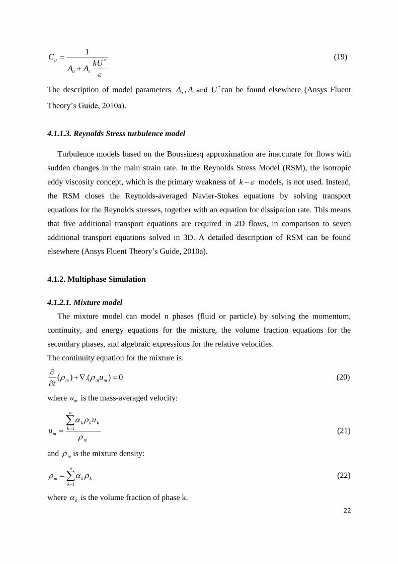
4.1.1.3. Reynolds Stress turbulence model

Turbulence models based on the Boussinesq approximation are inaccurate for flows with

sudden changes in the main strain rate. In the Reynolds Stress Model (RSM), the isotropic

eddy viscosity concept, which is the primary weakness of k models, is not used. Instead,

the RSM closes the Reynolds-averaged Navier-Stokes equations by solving transport

equations for the Reynolds stresses, together with an equation for dissipation rate. This means

that five additional transport equations are required in 2D flows, in comparison to seven

additional transport equations solved in 3D. A detailed description of RSM can be found

elsewhere (Ansys Fluent Theory‟s Guide, 2010a).

4.1.2. Multiphase Simulation

4.1.2.1. Mixture model

The mixture model can model n phases (fluid or particle) by solving the momentum,

continuity, and energy equations for the mixture, the volume fraction equations for the

secondary phases, and algebraic expressions for the relative velocities.

The continuity equation for the mixture is:

0).()(

mmm u

t (20)

where mu is the mass-averaged velocity:

m

n

k

kkk

m

u

u

1 (21)

and m is the mixture density:

n

k

kkm

1

(22)

where k is the volume fraction of phase k.

23

The momentum equation for the mixture can be obtained by summing the individual

momentum equations for all phases according to:

).()(.).()( ,

1

, kdr

n

k

kdrkkm

T

mmmmmmmm uuFguupuuut

(23)

where n is the number of phases, F is a body force, and m is the viscosity of the mixture:

k

n

k

km

1

(24)

where kdru , is the drift velocity for the secondary phase k:

mkkdr uuu , (25)

The energy equation for the mixture takes the following form:

).())((.)(11

TkpEuEt

effkk

n

k

kkkk

n

k

k

(26)

where effk is the effective conductivity (Ansys Fluent Theory‟s Guide, 2010b).

4.2. Flow Simulation

The geometry of the 2.5 L laboratory baffled stirred tank bioreactor (Biostat A., B. Braun

Biotech, Germany) used in this work with its all internal dimensions is presented in Table 3.

A Rushton turbine impeller was used to mix the content of the bioreactor. The impeller

rotated with a rotational speed of 200 rpm. Tetrahedral grids of ~ 555857 elements were

constructed for the entire bioreactor using Mixsim® 2.0, and Fluent

® 6.3.26 was used for

simulation of flow within the tank. The multiple reference frame (MRF) technique was used

to simulate the impeller motion. Both turbulence models including Realizable k-ε and

Reynolds stress with standard wall functions were used to model the flow profile inside the

bioreactor. The walls of the tank, baffles, and the other bioreactor internals were assigned the

standard wall function boundary condition. The model was allowed to run using double-

precision calculation until all the scaled residuals reached a value of 10-5

(Paper V).

4.3. Simulation of Yeast Flocs’ Distribution

Two interesting phases in this work were water and yeast flocs. The mixture approach was

used to calculate the interaction between these two phases and the volume fraction

distribution of yeast flocs. The cell concentration was low and the RANS models for flow

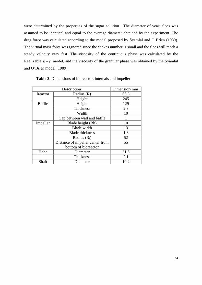
24

were determined by the properties of the sugar solution. The diameter of yeast flocs was

assumed to be identical and equal to the average diameter obtained by the experiment. The

drag force was calculated according to the model proposed by Syamlal and O‟Brien (1989).

The virtual mass force was ignored since the Stokes number is small and the flocs will reach a

steady velocity very fast. The viscosity of the continuous phase was calculated by the

Realizable k model, and the viscosity of the granular phase was obtained by the Syamlal

and O‟Brien model (1989).

Table 3. Dimensions of bioreactor, internals and impeller

Description Dimension(mm)

Reactor Radius (R) 66.5

Height 245

Baffle Height 129

Thickness 2.3

Width 10

Gap between wall and baffle 1

Impeller Blade height (Bh) 10

Blade width 13

Blade thickness 1.8

Radius (Ri) 52

Distance of impeller center from

bottom of bioreactor

55

Hobe Diameter 31.5

Thickness 2.1

Shaft Diameter 10.2

25

5. Results and Discussion

5.1. Enzymatic Hydrolysis

The ground CW was hydrolyzed using a mixture of enzymes at 45ºC for 24h with 12%

solid concentration. The respective loadings of pectinase, cellulase and β-glucosidase were

1163 IU/g, 0.24 FPU/g and 3.9 IU∕g CW dry matter, based on optimized values previously

reported by Wilkins et al. (2007c). The yields of sugars liberated after the hydrolysis are

summarized in Table 4. The released materials during the enzymatic hydrolysis were glucose,

fructose, galactose, arabinose, xylose and galacturonic acid (GA). Concentration of limonene

in the hydrolyzate was 0.52% (v/v) (Paper I).

Table 4. Yields of the carbohydrates released during enzymatic hydrolysis of the citrus

waste. The experiments were run in duplicate.

Carbohydrate % (of total solid)

Glucose 22.9 ± 2.4

Fructose 14.1 ± 1.3

Galactose 4.0 ± 0.2

Arabinose 7.1 ± 0.5

Xylose 0.4 ± 0.1

Galacturonic acid 19.0 ± 1.7

Total 67.5

26

The hydrolyzate was supplemented with nutrients and anaerobically cultivated by both freely

suspended and encapsulated S. cerevisiae. The suspended cells were not able to ferment the

hydrolyzate in 24 h, where no sugars could be taken up by S. cerevisiae and no ethanol was

produced. Since limonene is a hydrophobic component, it can pass freely through the cell wall

of yeast and inhibit lipid body formation and accumulation inside the cell (Bishop et al., 1998;

Kimura et al., 2006). The measured number of viable cells was practically zero after 4 h

cultivation (Paper I).

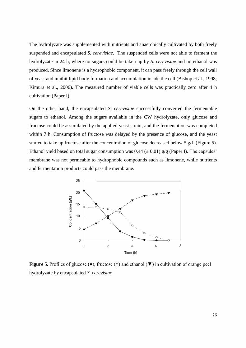
On the other hand, the encapsulated S. cerevisiae successfully converted the fermentable

sugars to ethanol. Among the sugars available in the CW hydrolyzate, only glucose and

fructose could be assimilated by the applied yeast strain, and the fermentation was completed

within 7 h. Consumption of fructose was delayed by the presence of glucose, and the yeast

started to take up fructose after the concentration of glucose decreased below 5 g/L (Figure 5).

Ethanol yield based on total sugar consumption was 0.44 (± 0.01) g/g (Paper I). The capsules‟

membrane was not permeable to hydrophobic compounds such as limonene, while nutrients

and fermentation products could pass the membrane.

Figure 5. Profiles of glucose (●), fructose (○) and ethanol (▼) in cultivation of orange peel

hydrolyzate by encapsulated S. cerevisiae

27

5.2. Process based on Dilute Acid Hydrolysis

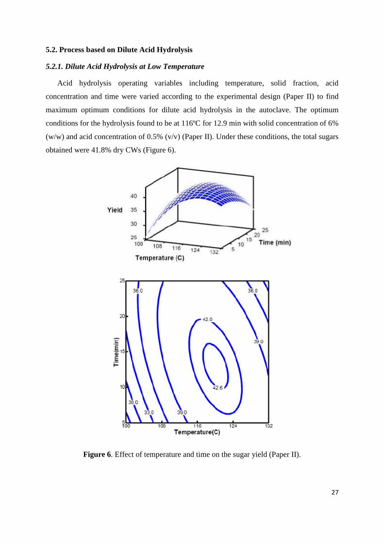
5.2.1. Dilute Acid Hydrolysis at Low Temperature

Acid hydrolysis operating variables including temperature, solid fraction, acid

concentration and time were varied according to the experimental design (Paper II) to find

maximum optimum conditions for dilute acid hydrolysis in the autoclave. The optimum

conditions for the hydrolysis found to be at 116ºC for 12.9 min with solid concentration of 6%

(w/w) and acid concentration of 0.5% (v/v) (Paper II). Under these conditions, the total sugars

obtained were 41.8% dry CWs (Figure 6).

Figure 6. Effect of temperature and time on the sugar yield (Paper II).

28

However, it should be considered that heating the slurry up to the hydrolysis temperature, and

the cooling the slurry before leaving from the autoclave took extra times which might have an

effect on the sugar yield. Furthermore, the limonene remains in hydrolyzate which stops the

following fermentation process.

5.2.2. Dilute Acid Hydrolysis at High Temperature

These experiments were carried out in the hydrolysis reactor and led to an optimum

temperature of 150 ºC and time of 6 min where acid and solid concentrations were 0.5% (v/v)

and 15% (w/w), respectively (Figure 7). Under these conditions, the best sugar yield of 0.41

g/g dry CW was obtained. While the sugar yield is similar with the results obtained by the

dilute acid hydrolysis in autoclave, the main advantage by using this process is that 99% of

the limonene content of CWs was released during the hydrolysis process and flashed in the

expansion tank (Paper III). The limonene can be recovered by condensation of vapor outlet of

the flash drum.

Figure 7. Effect of temperature and time on the yield of total sugars.

29

5.2.3. Fermentation

The hydrolyzate was centrifuged to separate non-soluble solids and after that supplemented

with nutrients and fermented anaerobically by the flocculating yeast. The concentration of

different sugars prior to the fermentation was 15.17, 10.88, 2.91 and 4.01 g/l for glucose,

fructose, galactose and arabinose, respectively. The yeast was not able to ferment arabinose,

but able to assimilate the hexoses. The fermentation was completed in 24 h, in which all the

fermentable sugars were consumed and ethanol was produced (Figure 8). Ethanol yield based

on total fermentable sugar consumption was 0.43 g/g. Glycerol and succinic acid were the

identified byproducts, which had yields of 0.10 and 0.006 g/g of fermentable sugars,

respectively. Ethanol was distilled at 96°C and the produced stillage and non-soluble solids

from the centrifuge were mixed and used as „substrate‟ for anaerobic digestion.

Time (h)0 5 10 15 20

Concentr

ation (

g/l)

0

5

10

15

20

25

30

Figure 8. Profile of total fermentable sugars (●) and ethanol (○) in cultivation of CW

hydrolyzate by S. cerevisiae.

5.2.4. Pectin Recovery

Pectin was not hydrolyzed to its sugar monomer „galacturonic acid‟ even at very high

temperatures, but it was solubilized during the hydrolysis process and consequently, it can be

precipitated using ethanol. The hydrolysis at 150°C for 6 min resulted in solubilization of

83.5% of the pectin present in CW, while 16.5% of the pectin still remained in the solid

fraction of the hydrolyzate. This high solubilization might be due to the applied high

temperature and the low pH during the hydrolysis. Precipitation of pectin content of the

hydrolyzate liquid resulted in recovery of pectin with a total of 77.6% of pectin content of

30

CWs. The degree of esterification and the ash content of recovered pectin were 63.7 (±0.98)

and 4.23 (±0.08) %, respectively.

5.2.5. Methane Production

The substrate for the anaerobic digestion had TS and VS contents of 4.6% and 4.3%,

respectively. The cumulative methane yield was 0.28 l/g VS after 10 days of incubation and

reached a constant level of 0.36 l/g VS after 30 days. More than 90% of the maximum

produced methane was achieved between 15 and 20 days. Compositions of methane and

carbon dioxide in the produced biogas were 41% and 59% (v/v), respectively.

5.2.6. Overall Process

By applying the process based on dilute acid hydrolysis, 39.64 l ethanol, almost 45 m3 pure

methane, 8.9 l limonene, and up to maximum 38.8 kg pectin can be produced per ton of the

wet CW. It is an integrated process, in which the ethanol produced in the process can be used

for pectin recovery, and the produced methane can be utilized in a steam boiler to generate

steam required for distillation and hydrolysis (Paper III) (Figure 9).

Hydrolysis Reactor

Expansion Tank Condenser/Decanter

Filter

Biogas Digester

Fermenter

Distillation

Citrus Waste

Sulfuric Acid

Limonene

Biogas

LiquidSolid

Steam

Water

Stillage

Hydrolysate

Precipitator

Dryer

Dried Pectin

Pectin

Ethanol

Pectin Depleted

Residue

Figure 9. Block flow diagram for production of ethanol, biogas, pectin and limonene from

CW.

31

5.3. Process Detail for Large-Scale Utilizing of Citrus Wastes

In this section, the conceptual design and economic analysis of the process based on dilute

acid hydrolysis with ethanol, limonene and methane as product (Figure 3) is presented.

5.3.1. Material Balance

A simplified material balance for a plant with capacity of „„100,000‟‟ tons CW/year is

provided in Table 5.

Table 5. Composition of streams involved in the process (Figure 3) for the base case capacity

of 100,000 tons citrus waste per year

Stream 1 2 3 4 5 6 7 8 9 10 11

Hexosans 0.650 - - - - - - - - - -

Pentosans 0.175 - - - - - - - - - -

Pectin 0.625 - - - - 0.525 - - - - -

Hexoses 0.570 - - - - 0.947 - - - - -

Pentoses - - - - - 0.090 - - - - -

Water 10 0.001 1.742 4.100 0.014 15.02 - 0.738 - - -

Sulfuric acid - 0.048 - - - - - - - - -

Limonene 0.125 - - - 0.125 - - - - - -

Ethanol - - - - - - - - 0.390 - -

Yeast - - - - - - 0.006 - - - -

Other 0.355 - - - - 0.178 - - - - -

- -

Total (ton/h) 12.5 0.049 1.742 4.100 0.11 16.76 0.006 0.738 0.390 - -

Methane (Nm3/h) - - - - - - - - - 558 397.5

CO2 (Nm3/h) - - - - - - - - - 803 8

5.3.2. Energy Analysis

The required steam of the process can be provided by burning 29% of the produced

methane in a steam boiler. The hydrolysis and distillation stages consume 70% and 30% of

total steam requirements (Paper IV). The electricity required for fermenters, digesters and

32

auxiliary equipment for the base case capacity is 0.837 MW, and it changes almost linearly

with plant capacity.

5.3.3. Fixed Capital Cost (FCI)

The fixed capital cost of the process for a plant with the base capacity was estimated to be

23.365 mUSD at 2009 (Figure 10). Doubling the plant capacity from base case to 200,000

tons CW/year results in 58% increase in FCI. Further increase in plant capacity to 400,000

tons CW/year makes this investment 67% higher than for the previous case. This higher

increase in FCI is due to number duplicating of biogas digesters rather than expansion at

higher capacities.

Figure 10. Plant fixed capital cost versus CW capacity

Figure 11 shows the contribution of each process step in the FCI. The anaerobic digestion

area, including biogas upgrading system, has the largest contribution, 31% of the total FCI.

The hydrolysis has the second largest contribution in FCI.

33

13%

8%

12%

31%

4%

6%

26%

Hydrolysis

Fermentation

Distillation

Anaerobic digestion

Waste water treatment

Utilities and storage

Other costs

Figure 11. Distribution of capital cost invested among different plant sections.

5.3.4. Cost of Manufacturing

Manufacturing cost of the plant is calculated as a sum of expenses of chemicals, utilities,

labor wages, maintenance and plant insurance. Table 6 shows the yearly manufacturing costs.

Table 6. Manufacturing costs for proposed CW capacities

Plant Capacity (ton CW/h)

Manufacturing Cost

(mUSD/year)

2.5

5.75

11.50

23.00

46.00

92.00

Chemicals & Yeast 0.18 0.41 0.81 1.66 3.32 6.65

Utilities 0.045 0.09 0.18 0.36 0.71 1.41

Labor

(No. of labor)

1.05

(15)

1.19

(17)

1.33

(19)

1.47

(21)

1.68

(24)

1.89

(27)

Insurance

(1% of CTCI)

0.10 0.13 0.15 0.23 0.37 0.61

Maintenance

(2% of CTCI)

0.20 0.27 0.31 0.46 0.74 1.23

5.3.5. Ethanol Production Cost

34

By considering biogas and peel oil as by-products of the plant, an ethanol production cost

was calculated as a measure of the production cost corresponding to 15 years plant life and

minimum 5% return on investment. Figure 12 shows the breakdown of the ethanol production

cost by assuming an average transportation cost of 10 USD/ton for the CW. The main costs

are those for capital and labor. By doubling the plant capacity from the base case to 200,000

tons CW per year, the major costs associated with raw materials, energy consumption and

utilities are almost doubled resulting in about the same expenses per liter of ethanol in

different capacities. The capital cost of the plant does not change linearly with the plant size

(Figure 10). Therefore, the effect of capital cost on the ethanol production cost is not the same

for all capacities and decreases when the plant capacity increases (Figure 12). Labor cost is

the second significant expense among production cost components, which is not doubled by

the plant capacity. The numbers of plant operators and labor supervisors needed per shift are

based on the type and arrangement of the equipment rather than the capacity of the plant.

Therefore, the effect of labor costs is more significant at lower capacities (Figure 12). In this

process, the steam requirement is fulfilled by burning 29% of the produced methane, which

results in low utility cost compared to the total operating cost (Figure 12).

-0.5

0

0.5

1

1.5

2

2.5

3

Plant capacity (tons citrus waste/Year)

Eth

an

ol

pro

du

cti

on

co

st

($/L

)

Total

Chemicals

Utilities

Labor

Maintenance &

InsuranceBiogas

Limonene

Feedstock

TransportationCapital

25,000 50,000 100,000 200,000 400,000

Figure 12. Cost breakdown of ethanol production for different plant scenarios.

The production cost of ethanol for different plant processing capacities and feed

transportation costs is presented in Figure 13. Assuming no transportation cost, production

cost of ethanol at plant capacities lower than 65,000 tons CW per year will be higher than 1.0

35

USD per liter of produced ethanol. It was also found that doubling the plant capacity from the

base case reduces the production cost by 43% to 0.38 USD/L. The feed transportation cost is

an important factor in ethanol production cost. For comparison, decreasing the feed

transportation cost from 30 to 10 USD/ton can reduce ethanol production cost by 36% for the

base case (Figure 13).

Figure 13. Ethanol production cost as function of plant size and feedstock transportation cost.

5.3.6. Comparison with Previous Processes

Previous researchers (Stewart et al., 2006; Zhou et al., 2007) have reported a process for

production of ethanol from CW based on enzymatic hydrolysis with a yield of ethanol that is

almost 35% higher than that obtained in our process (Stewart et al., 2006). However, their

process suffers from high price for the enzymes and high demand of energy in the distillation,

evaporators and dryer. In contrast, the process reported in this thesis does not consume

enzymes and the steam requirement can be provided by burning some part of the produced

methane. Furthermore, this process can be easily combined with a biogas plant or an ethanol

factory. This could decrease the FCI of the process and make it feasible to produce ethanol

even at low CW capacities.

5.4. Process Details for Low-Scale Utilizing of Citrus Waste

The production of ethanol through dilute acid hydrolysis process seems to be feasible at

CW capacities higher than 100,000 tons/year (Figure 13). For juice factories with lower

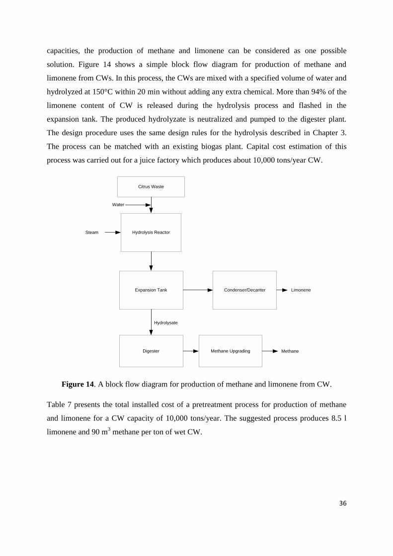
36

capacities, the production of methane and limonene can be considered as one possible

solution. Figure 14 shows a simple block flow diagram for production of methane and

limonene from CWs. In this process, the CWs are mixed with a specified volume of water and

hydrolyzed at 150°C within 20 min without adding any extra chemical. More than 94% of the

limonene content of CW is released during the hydrolysis process and flashed in the

expansion tank. The produced hydrolyzate is neutralized and pumped to the digester plant.

The design procedure uses the same design rules for the hydrolysis described in Chapter 3.

The process can be matched with an existing biogas plant. Capital cost estimation of this

process was carried out for a juice factory which produces about 10,000 tons/year CW.

Limonene

Hydrolysis Reactor

Expansion Tank Condenser/Decanter

Digester

Citrus Waste

Steam

Hydrolysate

Water

Methane Upgrading Methane

Figure 14. A block flow diagram for production of methane and limonene from CW.

Table 7 presents the total installed cost of a pretreatment process for production of methane

and limonene for a CW capacity of 10,000 tons/year. The suggested process produces 8.5 l

limonene and 90 m3 methane per ton of wet CW.

37

Table 7. Installed cost of process equipments required for treatment of CW.

Equipment Installed Cost (1000USD)

Reactors 89

Flash Drum 435

Condenser 95

Decanter 63

Pump 48

Conveyor 103

Container 46

Total Cost 879

5.5. Computational Fluid Dynamics Simulation Results

5.5.1. Flow Simulation

Two turbulence models, „Reynolds Stress‟ and „Realizable k-ε‟, were used to study

turbulence in the laboratory bioreactor. Turbulence properties such as energy dissipation,

kinetic energy and turbulence intensity were investigated particularly (Paper V). Furthermore,

velocities predicted by the two models were compared.

5.5.1.1. Turbulence Intensity

The distribution of turbulence intensity has been provided in Figure 15. Both turbulence

models predict the same trend of turbulence intensities; however, the values predicted by

Realizable k-ε were higher than the values obtained by the Reynolds Stress model. The

differences in values predicted by the two models decreased in the near wall region. The

turbulence intensities calculated by both models were lower than the experimental data (Wu

and Patterson, 1989). Wu and Patterson (1989) reported a maximum turbulence intensity

around 0.5Utip which corresponds to a maximum turbulent kinetic energy of 0.125 (Utip)2.

38

Dimensionless Radial Coordinate,(r-Ri)/(R-Ri)

0.0 0.2 0.4 0.6 0.8 1.0

Tu

rbu

len

ce

In

ten

sit

y,

U/U

tip

0.02

0.04

0.06

0.08

0.10

0.12

0.14

Figure 15. The turbulence intensity predicted by Realizable k-ε (●) and Reynolds Stress (○)

at the impeller central plane (Paper V).

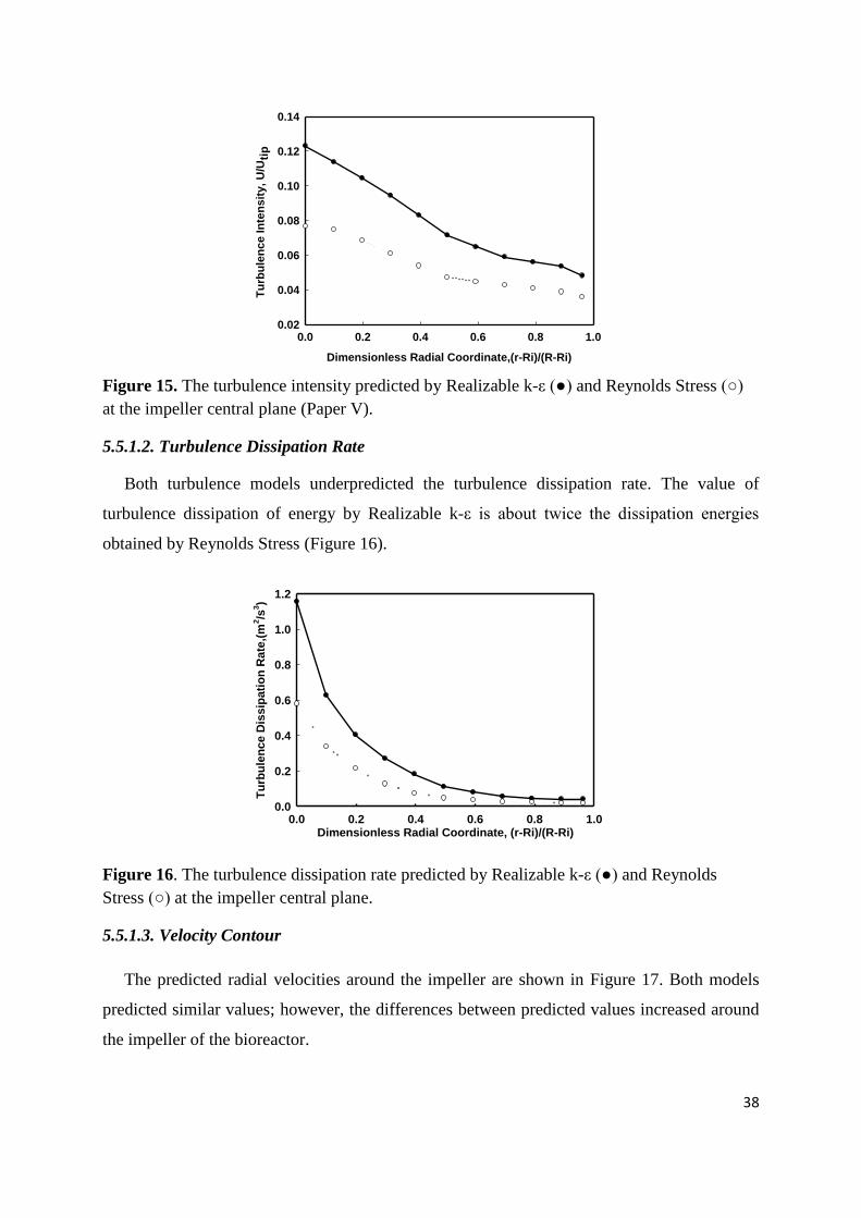
5.5.1.2. Turbulence Dissipation Rate

Both turbulence models underpredicted the turbulence dissipation rate. The value of

turbulence dissipation of energy by Realizable k-ε is about twice the dissipation energies

obtained by Reynolds Stress (Figure 16).

Dimensionless Radial Coordinate, (r-Ri)/(R-Ri)0.0 0.2 0.4 0.6 0.8 1.0

Tu

rbu

len

ce D

issip

ati

on

Rate

,(m

2/s

3)

0.0

0.2

0.4

0.6

0.8

1.0

1.2

Figure 16. The turbulence dissipation rate predicted by Realizable k-ε (●) and Reynolds

Stress (○) at the impeller central plane.

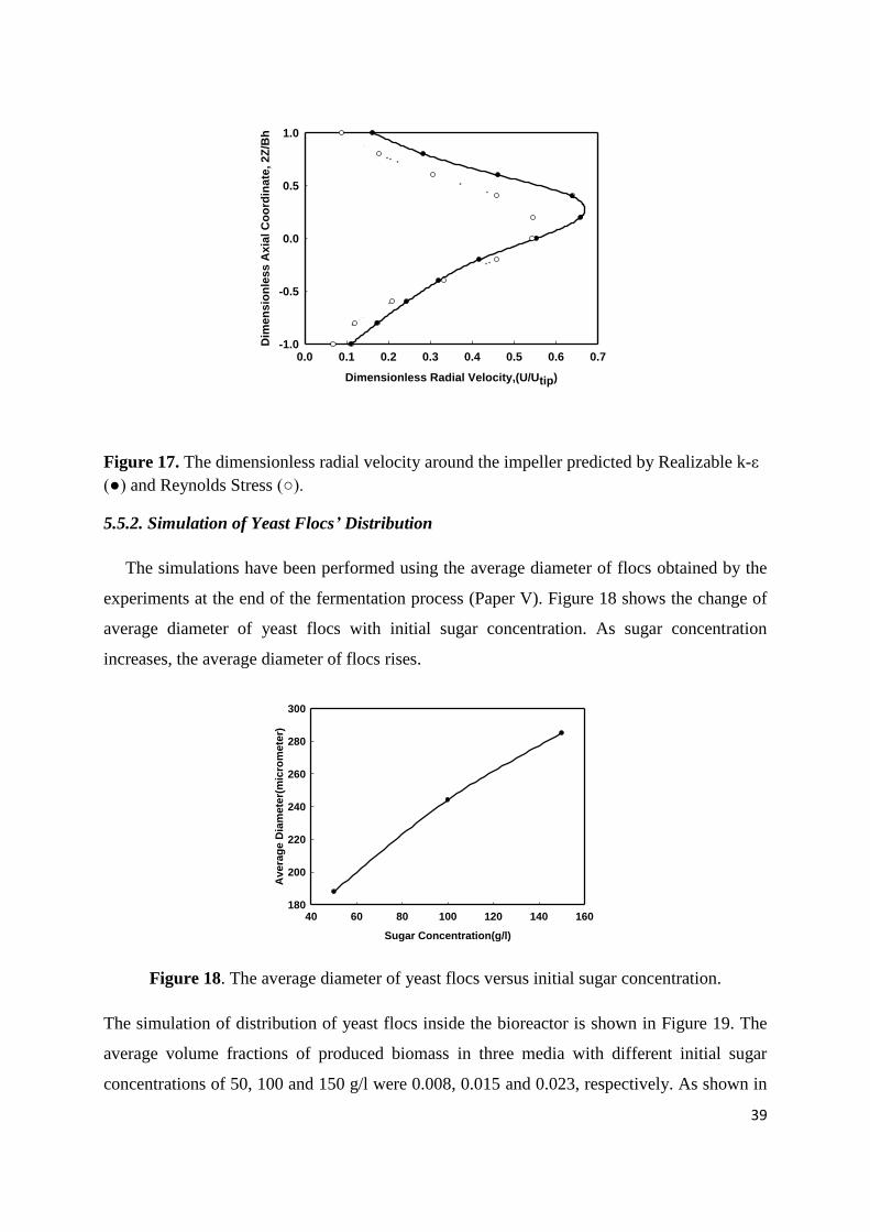
5.5.1.3. Velocity Contour

The predicted radial velocities around the impeller are shown in Figure 17. Both models

predicted similar values; however, the differences between predicted values increased around

the impeller of the bioreactor.

39

Dimensionless Radial Velocity,(U/Utip)

0.0 0.1 0.2 0.3 0.4 0.5 0.6 0.7

Dim

en

sio

nle

ss

Axia

l C

oo

rdin

ate

, 2

Z/B

h

-1.0

-0.5

0.0

0.5

1.0

Figure 17. The dimensionless radial velocity around the impeller predicted by Realizable k-ε

(●) and Reynolds Stress (○).

5.5.2. Simulation of Yeast Flocs’ Distribution

The simulations have been performed using the average diameter of flocs obtained by the

experiments at the end of the fermentation process (Paper V). Figure 18 shows the change of

average diameter of yeast flocs with initial sugar concentration. As sugar concentration

increases, the average diameter of flocs rises.

Sugar Concentration(g/l)

40 60 80 100 120 140 160

Av

era

ge D

iam

ete

r(m

icro

mete

r)

180

200

220

240

260

280

300

Figure 18. The average diameter of yeast flocs versus initial sugar concentration.

The simulation of distribution of yeast flocs inside the bioreactor is shown in Figure 19. The

average volume fractions of produced biomass in three media with different initial sugar

concentrations of 50, 100 and 150 g/l were 0.008, 0.015 and 0.023, respectively. As shown in

40

the figure, the distribution of flocs inside the bioreactor seems to be more homogeneous with

lower initial sugar concentrations. In fact, when the yeast concentration increases, the yeast

floc sedimentation also increases. This was in agreement with what was observed in the

experiments.

During the fermentation process, the flocculabilty of the yeast cells increases due to

decreasing sugar concentration (Smit et al., 1992). Thus, very large flocs are formed during

the fermentation process and the power input (mixer speed rate) is not enough to circulate the

flocs and consequently, they sediment (Figure 19).

A B C

Figure 19. Volume fraction distribution of yeast flocs inside the laboratory bioreactor as

predicted by CFD. Sugar concentrations (g/l): A:50, B:100 and C:150.

41

6. Conclusion

In this work, the production of ethanol and other sustainable products from CWs was

studied. The CWs were hydrolyzed using a mixture of enzymes and the hydrolyzate was

fermented by encapsulated cells. However, the application of the encapsulated cells may be

hampered by the high price of encapsulation and enzymes and the low stability of capsules‟

membrane at high shear stress.

Therefore, a process based on dilute acid hydrolysis of CWs was developed which produces

four products, limonene, pectin, ethanol and methane, from CWs. The process is an integrated

process whose energy is provided by burning some part of the produced methane. The

feasibility of this process is related to the capacity of CW and the transportation costs. This

process can be applied for the juice factories with CW capacities higher than 100,000

tons/year. The bioreactor used in the process employs a flocculating yeast strain. The size of

the yeast flocs is a function of flow, time and sugar concentration. The yeast flocs can

sediment if they are big enough. The CFD can be used to simulate the yeast flocs‟ distribution

in the bioreactor and predict the sedimentation of the yeast flocs.

On the other hand, if the capacity of the CW is low or the ethanol production is not feasible, a

steam explosion process can be employed to eliminate limonene and the treated CW can be

used in an anaerobic digestion plant to produce methane.

42

7. Future Work

The following suggestions could be of interest for future studies:

-Development of an economic model which predicts the effect of pectin production and size

of pectin plant on the feasibility of the process

-Study of a combination of dilute-acid pretreatment and enzymatic hydrolysis of CW and

economic analysis of the process

- Optimization of pectin production and study effect of changes in acid concentration and

temperature on the quality of produced pectin.

- Study of the possibilities of integrating processes developed in this work with existing

ethanol plants or digestion plants

43

NOMENCLATURE

Abbreviations

COM Cost of manufacturing

CTIC Total installed cost

CTDC Total depreciable cost

CFD Computational fluid dynamics

CW Citrus Waste

DCFA Discounted cash flow analysis

DE Degree of esterification

FCI Fixed Capital Investment

HMF Hydroxymethylfurfural

MRF Multiple reference frame

NPV Net present value

RANS Reynolds Average Navier Stocks

RSM Reynolds Stress Model

SSF Simultaneous saccharification and fermentation

Variables, constants and parameters

A0 Parameter in the Realizable k-ε model

As Parameter in the Realizable k-ε model

Bh Blade height [10-3

m]

C Price [USD]

C1 Closure coefficient in the Realizable k-ε model

C2 Closure coefficient in the Realizable k-ε model

C1ε Closure coefficient in the Realizable k-ε model

C3ε Closure coefficient in the Realizable k-ε model

d Average floc diameter [10-6

m]

dc Single yeast diameter [10-6

m]

44

D Fractal dimension [-]

E Energy [J]

g Gravity constant [m/s2]

Gk The generation of turbulence kinetic energy due to the mean velocity gradient[W/m3]

Gb The generation of turbulence kinetic energy due to buoyancy [W/m3]

k Turbulence kinetic energy per unit mass [J/kg]

kf Effective conductivity[W/m/K]

P Pressure [Pas]

Q Wastewater flow [Gal/min]

R Reactor radius [10-3

m]

Ri Impeller radius [10-3

m]

Sij Mean rate of strain tensor [s-1

]

T Temperature [K]

t Time[s]

U Mean velocity [m/s]

U* Parameter in the Realizable k-ε model

u Instantaneous velocity [m/s]

u΄ Fluctuating part of velocity [m/s]

udr Drift velocity [m/s]

um Mixture velocity [m/s]

uk Velocity of phase k [m/s]

V Settling velocity [m/s]

X Plant capacity [tons/year]

Y Operating-labor-hours per ton of product [h/ton]

YM Closure in the Realizable k-ε model

Greek Letters

ε Turbulence dissipation rate [m2/s

3]

45

σk Prandtl number [-]

σε Prandtl number [-]

ν Viscosity [kg/m/s]

νT Turbulent viscosity [m2/s

2]

η Parameter in the Realizable k-ε model

αk Volume fraction of phase k [-]

τs Shear stress [kg/s2/m]

μ Viscosity [kg/m/s]

μk Viscosity of phase k [kg/m/s]

μm Mixture viscosity [kg/m/s]

ρ Density [kg/m3]

ρk Density of phase k [kg/m3]

ρm Mixture density [kg/m3]

ρy Yeast density [kg/m3]

ρl Medium density [kg/m3]

Density difference between a yeast floc and the culture medium [kg/m3]

The volume fraction of particles [-]

46

ACKNOWLEDGEMENT

I would like to express my warm thanks to all the people who have helped me in this work:

My supervisor, Professor Mohammad Taherzadeh, for giving me excellent advice,

encouragement and helping me in articles.

Special thanks to my co-supervisor, Professor Bengt Andersson, who taught me

computational fluid dynamics simulation and opened new windows for me in understanding

Chemical Reaction Engineering.

My examiner, Professor Claes Niklasson, for helping me during this four-year journey and for

all encouragement and support.

Dr. Britt-Marie Steenari, director of Graduate School of Chemical Engineering, and Dr.

Christer Larsson for helping me with the organization of my PhD work.

I would like to express my deep gratitude to all the people at the School of Engineering at

University of Borås for contributing to a pleasant atmosphere. Dr. Peter Therning, Dr. Hans

Björk, Dr. Dag Henriksson – thank you all for your openness toward me and for your

collaboration. I would also like to thank other colleagues and friends, Jonas, Anna, Akram,

Azam, Tatiana, Patrik, Solmaz, Thomas and Dan.

Inicia AB is appreciated for helping us in patenting part of this work. Thanks to the

Foundation of Swedbank in Sjuhärad, Sjuhärad Association of Local Authorities (Sweden),

and to the Swedish Energy Agency for financial support of this work and the research school

of POWRES financed by Formas.

Marianne Sognell for all help, PhD students at CRE, Andreas, Henrik and Carl for helping me

in CFD, my colleagues Mehdi and Gergely for contributing in this work, Dr Ilona Sárvári

Horváth and Dr. Farid Talebnia for contributing and helping me in research.

Professor Srdjan Sasic, Professor William George, Professor Derek Creaser, Professor Anders

Rasmusson, Professor Bengt Andersson, Dr. Magnus Lundin, and Dr. Louise Olsson for their

excellent courses.

My great thanks to my parents and my best friend Mohammad Baniassadi who have

supported me during these years.

47

REFERENCES

Andersson B., Andersson R., Håkansson L., Mortensen M., Sudiyo R., Van Wachem B.,

Computational Fluid Dynamics for Chemical Engineers, Chalmers Publication, Fourth

Edition, 2008.

Ansys Fluent Theory's Guide, 2010a, Chapter 4, Turbulence.

Ansys Fluent Theory's Guide, 2010b, Chapter 16, Multiphase Flows.

Aravantinoszafiris, G., Oreopoulou, V. (1992). The effect of nitric acid extraction variables

on orange pectin. Journal of the Science of Food and Agriculture, 60, 127-129.

Bishop, J.R.P., Nelson, G., Lamb, J. (1998). Microencapsulation in yeast cells. Journal of

Microencapsulation, 15, 761-773.

Decker, S. R., Adney, W. S., Jennings, E., Vinzant, T. B. and Himmel, M. E. (2003).

Automated filter paper assay for determination of cellulase activity. Applied

Biochemistry and Biotechnology, 105, 689-703.

Faravash, R.S., Ashtiani, F.Z. (2007). The effect of pH, ethanol volume and acid washing

time on the yield of pectin extraction from peach pomace. International Journal of

Food Science and Technology, 42, 1177-1187.

Fernandez, A., Sanchez A., Font X. (2005). Anaerobic co-digestion of a simulated organic

fraction of municipal solid wastes and fats of animal and vegetable origin.

Biochemical Engineering Journal, 26, 22-28.

Galbe, M., Sassner, P., Wingren, A., Zacchi, G. (2007). Process engineering economics for

bioethanol production. Advances in Biochemical Engineering Biotechnology, 108,

303-327.

Ge, X. M., Zhang, L. and Bai, F. W. (2006). Impacts of yeast floc size distributions on their

observed rates for substrate uptake and product formation. Enzyme and Microbial

Technology, 39, 289-295.

Grohmann, K. and Baldwin, E. A. (1992). Hydrolysis of orange peel with pectinase and

cellulase enzymes. Biotechnology Letter, 14, 1169-1174.

Grohmann, K., Baldwin, E. A. and Buslig, B. S. (1994). Production of ethanol from

enzymatically hydrolyzed orange peel by the Yeast Saccharomyces cerevisiae.

Applied Biochemistry and Biotechnology, 45-6, 315-327.

Grohmann, K., Cameron, R. G. and Buslig, B. S. (1995). Fractionation and pretreatment of

orange peel by dilute acid hydrolysis. Bioresource Technology, 54, 129-141.

48

Hansen, T. L., Schmidt, J. E., Angelidaki, I., Marca, E., Jansen, J. L., Mosbaek, H. and

Christensen, T. H. (2004). Method for determination of methane potentials of solid

organic waste. Waste Management, 24, 393-400.

Kadam, K.L., Wooley, R., Aden, A., Nguyen , Q. A., Yancey , M.A. and Ferraro, F.M.(2000).

Softwood forest thinnings as a biomass source for ethanol production: A feasibility

study for California. Biotechnology Progress, 16, 947-957.

Kimura, K., Yamaoka, M., Kamisaka, Y. (2006) Inhibition of lipid accumulation and lipid

body formation in Oleaginous yeast by effective components in Spices, Carvacrol,

Eugenol, Thymol and Piperine. Journal of Agricultural Food and Chemistry, 54,

3528-3534.

Marin, F.R., Soler-Rivas, C., Benavente-Garcia, O., Castillo, J., Perez-Alvarez, J.A. (2007).

By-products from different citrus processes as a source of customized functional

fibers. Food Chemistry, 100, 736-741.

Monou, M., Pafitis, N., Kythreotou, N., Smith, S. R., Mantzavinos, D. and Kassinos, D.

(2008). Anaerobic co-digestion of potato processing wastewater with pig slurry and

abattoir wastewater. Journal of Chemical Technology and Biotechnology, 83, 1658-

1663.

Montgomery, D. C. (2001). Design and analysis of experiments, John Wiley and Sons, New

York, 427-450.

Nguyen, Q.A., Saddler, J.N. (1991). An integrated model for technical and economic

evaluation of an enzymatic biomass conversion process. Bioresource Technology, 35,

275-282.

Perlack, R. D., Wright, L. L., Turhollow, A. F., Graham, R. L., Stokes, B. J. and Erbach, D.

C. (2006). Biomass as feedstock for a bioenergy and bioproducts industry: The

technical feasibility of a billion-ton annual supply. Report ORNL/TM-2005/66. US

Department of Energy, Washington DC, USA.

Perry, R.H., Green, D.W. (1997). Perry's Chemical Engineers' Handbook. 7th ed. McGraw-

Hill Inc., New York.

Purwadi, R., Brandberg, T. and Taherzadeh, M. J. (2007). A possible industrial solution to

ferment lignocellulosic hydrolyzate to ethanol: Continuous cultivation with

flocculating yeast. International Journal of Molecular Science, 8, 920-932.

Ranganna, S. (1987). Handbook of analysis and quality control for fruit and vegetable

products. McGraw Hill Higher Education.

Sassner, P., Galbe, M. and Zacchi, G. (2008). Techno-economic evaluation of bioethanol

production from three different lignocellulosic materials. Biomass and Bioenergy, 32,

422-430.

49

Seider, W. D., Seader, J. D. and Lewin, D. R. (2004). Product & process design principles -

synthesis, analysis, and evaluation, John Wiley & Sons, Inc., New York.

Smit, G., Straver, M. H., Lugtenberg, B. J. J. and Kijne, J. W. (1992). Flocculence of

Saccharomyces cerevisiae cells is induced by nutrient limitation, with cell-surface

hydrophobicity as a major determinant. Applied and Environmental Microbiology, 58,

3709-3714.

Stewart, D.A., Widmer, W.W., Grohmann, K., Wilkins, M.R. (2005). Ethanol Production

from citrus processing waste, US Patent Application 11/052,620.

Syamlal, M. and O‟Brien, T. J. (1989). Computer simulation of bubbles in a fluidized bed.

AIChE Symp. Series, 85, 22-31.

Taherzadeh, M. J., Liden, G., Gustafsson, L. and Niklasson, C. (1996). The effects of

pantothenate deficiency and acetate addition on anaerobic batch fermentation of

glucose by Saccharomyces cerevisiae. Applied Microbiology and Biotechnology, 46,

176-182.

Talebnia, F., Niklasson, C. and Taherzadeh, M. J. (2005). Ethanol production from glucose

and dilute-acid hydrolyzates by encapsulated S-cerevisiae. Biotechnology and

Bioengineering, 90, 345-353.

Tripodo, M.M., Lanuzza, F., Micali, G., Coppolino, R., Nucita, F. (2004). Citrus waste

recovery: a new environmentally friendly procedure to obtain animal feed.

Bioresource Technology, 91, 111-115.

Turton, R., Bailie, R.C., Whiting, W.B., Shaeiwitz, J.A. (2003). Analysis, synthesis, and

design of chemical processes. 2nd ed. Prentice Hall PTR, Upper Saddle River, New

Jersey.

van Hamersveld, E. H., van der Lans, R. and Luyben, K. (1997). Quantification of brewers'

yeast flocculation in a stirred tank: Effect of physical parameters on flocculation.

Biotechnology and Bioengineering, 56, 190-200.

Ververis, C., Georghiou, K., Danielidis, D., Hatzinikolaou, D. G., Santas, P., Santas, R. and

Corleti, V. (2007). Cellulose, hemicelluloses, lignin and ash content of some organic

materials and their suitability for use as paper pulp supplements. Bioresource

Technology, 98, 296-301.

Wilkins, M. R., Suryawati, L., Maness, N. O. and Chrz, D. (2007a). Ethanol production by

Saccharomyces cerevisiae and Kluyveromyces marxianus in the presence of orange-

peel oil. World Journal of Microbiology and Biotechnology, 23, 1161-1168.

Wilkins, M. R., Widmer, W. W. and Grohmann, K. (2007b). Simultaneous saccharification

and fermentation of citrus peel waste by Saccharomyces cerevisiae to produce ethanol.

Process Biochemistry, 42, 1614-1619.

50

Wilkins, M. R., Widmer, W. W., Grohmann, K. and Cameron, R. G. (2007c). Hydrolysis of

grapefruit peel waste with cellulase and pectinase enzymes. Bioresource Technology,

98, 1596-1601.

Wingren, A., Galbe, M. and Zacchi, G. (2003a). Techno-economic evaluation of producing

ethanol from softwood: comparison of SSF and SHF and identification of bottlenecks,

Biotechnology Progress, 19, 1109-1117.

Wingren, A., Söderström, J., Galbe, M. and Zacchi, G. (2003b). Process considerations and

economic evaluation of two-step steam pretreatment for production of fuel ethanol

from softwood, Biotechnology Progress, 20, 1421-1429.

Wingren, A., Galbe, M., Roslander, C., Rudolf, A. and Zacchi, G. (2005), Effect of reduction

in yeast and enzyme concentrations in a simultaneous-saccharification and

fermentation based bioethanol process, Applied Biochemistry and Biotechnology, 121-

124,485-499.

Wooley, R. J., Ruth, M., Sheehan, J., Ibsen, K., Majdeski, H. and Galvez, A. (1999).

Lignocellulosic biomass to ethanol process design and economics utilizing co-current

dilute acid prehydrolysis and enzymatic hydrolysis current and futuristic scenarios.

NREL/TP-580-26157.

Wooley, R.J., Putsche, V., (1996). Development of an ASPEN PLUS physical property

database for Biofuels components. NREL/MP-425-20685.

Wu, H. and Patterson, G. K. (1989). Laser-Doppler measurements of turbulent-flow

parameters in a stirred mixer. Chemical Engineering Science, 44, 2207-2221.

Zhou, W., Widmer, W. and Grohmann, K. (2007). Economic analysis of ethanol production

from citrus peel waste. Proc Fla State Hort Soc, 120, 310-315.