CIPRES: Enabling Tree of Life Projects

Tandy Warnow

The University of Texas at Austin

Phylogeny

Orangutan Gorilla Chimpanzee Human

From the Tree of the Life Website,University of Arizona

Evolution informs about everything in biology

• Big genome sequencing projects just produce data – so what?

• Evolutionary history relates all organisms and genes, and helps us understand and predict – interactions between genes (genetic networks)

– drug design

– predicting functions of genes

– influenza vaccine development

– origins and spread of disease

– origins and migrations of humans

Reconstructing the “Tree” of Life

Handling large datasets: Handling large datasets: millions of species millions of species and and NP-hard optimization NP-hard optimization problemsproblems

NSF funds many projectsNSF funds many projectstowards this goal, undertowards this goal, underthethe Assembling the Tree of Assembling the Tree of Life Life programprogram

Cyber Infrastructure for Phylogenetic Research

Purpose: to create a national infrastructure of hardware, algorithms, database technology, etc., necessary to infer the Tree of Life. Group: approx. 36 biologists, computer scientists, and mathematicians from 18 institutions.Funding: $11.6 M (large ITR grant from NSF).

CIPRES Members

EPFL (Switzerland)Bernard Moret

Georgia TechDavid Bader

UCSD/SDSCFran Berman Alex Borchers John Huelsenbeck Terri LiebowitzMark Miller University of ConnecticutPaul O Lewis

University of PennsylvaniaJunhyong Kim Susan Davidson Sampath KannanVal Tannen

Texas A&MTiffani Williams

UT Austin Tandy Warnow David M. Hillis Warren Hunt Robert Jansen Randy Linder Lauren Meyers Daniel Miranker

University of ArizonaDavid R. Maddison

University of British ColumbiaWayne Maddison

North Carolina State UniversitySpencer Muse

American Museum of Natural HistoryWard C. Wheeler

NJITUsman Roshan

UC BerkeleySatish Rao Steve EvansRichard M Karp Brent MishlerElchanan MosselEugene W. MyersChristos M. PapadimitriouStuart J. Russell

Rice Luay Nakhleh

SUNY BuffaloWilliam Piel

Florida State UniversityDavid L. SwoffordMark Holder

Yale Michael DonoghuePaul Turner

CIPRES algorithms research (sample)

• Improved heuristics for NP-hard optimization problems (MP, ML, tree alignment)

• Obtaining better mathematical theory for phylogeny reconstruction methods under Markov models of evolution

• Supertree methods

• Constructing networks rather than trees (detecting and reconstructing reticulate evolution)

• Whole genome phylogeny

This talk

• Phylogeny reconstruction through a divide-and-conquer strategy using chordal graph theory– “Absolute fast converging” methods– Improved heuristics for NP-hard optimization

problems

DNA Sequence Evolution

AAGACTT

TGGACTTAAGGCCT

-3 mil yrs

-2 mil yrs

-1 mil yrs

today

AGGGCAT TAGCCCT AGCACTT

AAGGCCT TGGACTT

TAGCCCA TAGACTT AGCGCTTAGCACAAAGGGCAT

AGGGCAT TAGCCCT AGCACTT

AAGACTT

TGGACTTAAGGCCT

AGGGCAT TAGCCCT AGCACTT

AAGGCCT TGGACTT

AGCGCTTAGCACAATAGACTTTAGCCCAAGGGCAT

Phylogeny Problem

TAGCCCA TAGACTT TGCACAA TGCGCTTAGGGCAT

U V W X Y

U

V W

X

Y

1. Heuristics for NP-hard optimization criteria (Maximum Parsimony and Maximum Likelihood)

Phylogenetic reconstruction methods

Phylogenetic trees

Cost

Global optimum

Local optimum

2. Polynomial time distance-based methods: Neighbor Joining, FastME, etc.

3. Bayesian MCMC methods.

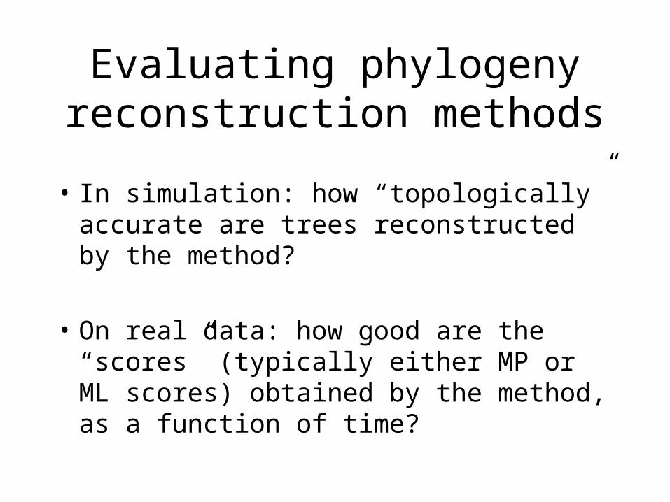
Evaluating phylogeny reconstruction methods

• In simulation: how “topologically” accurate are trees reconstructed by the method?

• On real data: how good are the “scores” (typically either MP or ML scores) obtained by the method, as a function of time?

DNA Sequence Evolution

AAGACTT

TGGACTTAAGGCCT

-3 mil yrs

-2 mil yrs

-1 mil yrs

today

AGGGCAT TAGCCCT AGCACTT

AAGGCCT TGGACTT

TAGCCCA TAGACTT AGCGCTTAGCACAAAGGGCAT

AGGGCAT TAGCCCT AGCACTT

AAGACTT

TGGACTTAAGGCCT

AGGGCAT TAGCCCT AGCACTT

AAGGCCT TGGACTT

AGCGCTTAGCACAATAGACTTTAGCCCAAGGGCAT

Markov models of DNA sequence evolution

General Time Reversible (GTR) Markov Model:• The state at the root is random • The model tree is a pair consisting of a rooted binary tree

T with edge lengths, where w(e) indicates the number of times a site changes on edge e.

• There is a 4x4 symmetric substitution matrix for the sites, so that if a site changes on an edge, it uses the matrix to determine the probability of each change.

• The evolutionary process is Markovian• All sites evolve identically and independently

Distance-based Phylogenetic Methods

Quantifying Error

FN: false negative (missing edge)FP: false positive (incorrect edge)

50% error rate

FN

FP

Neighbor joining has poor accuracy on large diameter model trees

[Nakhleh et al. ISMB 2001]

Simulation study based upon fixed edge lengths, K2P model of evolution, sequence lengths fixed to 1000 nucleotides.

Error rates reflect proportion of incorrect edges in inferred trees.

NJ

0 400 800 16001200No. Taxa

0

0.2

0.4

0.6

0.8

Err

or R

ate

Problems with current techniques for MP

0

0.02

0.04

0.06

0.08

0.1

0.12

0.14

0.16

0.18

0.2

0 4 8 12 16 20 24

Hours

Average MP score above

optimal, shown as a percentage of

the optimal

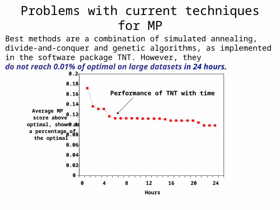
Shown here is the performance of the TNT software for maximum parsimony on a real dataset of almost 14,000 sequences. The required level of accuracy with respect to MP score is no more than 0.01% error (otherwise high topological error results). (“Optimal” here means best score to date, using any method for any amount of time.)

Performance of TNT with time

Empirical problems with existing methods

• Polynomial time methods have poor topological accuracy on large datasets – we need better polynomial time methods.

• Heuristics for Maximum Parsimony (MP) and Maximum Likelihood (ML) and Bayesian MCMC methods cannot handle large datasets (take too long!) – we need new heuristics that can analyze large datasets.

“Boosting” phylogeny reconstruction methods

• DCMs “boost” the performance of phylogeny reconstruction methods.

DCMBase method M DCM-M

Graph-theoretic divide-and-conquer (DCM’s)

• Define a triangulated (i.e. chordal) graph so that its

vertices correspond to the input taxa

• Compute a decomposition of the graph into overlapping subgraphs, thus defining a decomposition of the taxa into overlapping subsets.

• Apply the “base method” to each subset of taxa, to construct a subtree

• Merge the subtrees into a single tree on the full set of taxa.

Some properties of chordal graphs

• Every chordal graph has at most n maximal cliques, and these can be found in polynomial time: Maxclique decomposition.

• Every chordal graph has a vertex separator which is a maximal clique: Separator-component decomposition.

• Every chordal graph has a perfect elimination scheme: enables us to merge correct subtrees and get a correct supertree back, if subtrees are big enough.

A separator-component DCM (cartoon)

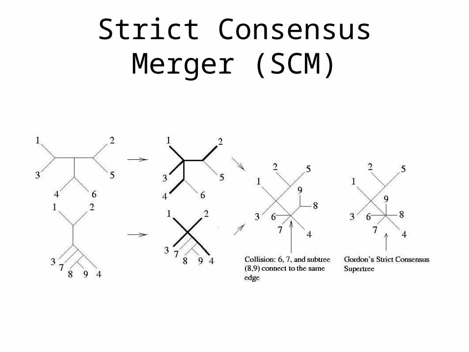
Strict Consensus Merger (SCM)

DCMs (Disk-Covering Methods)

• DCMs for polynomial time methods improve topological accuracy (empirical observation), and have provable theoretical guarantees under Markov models of evolution

• DCMs for hard optimization problems reduce running time needed to achieve good levels of accuracy (empirically observation)

Statistical consistency, convergence rates, and absolute fast convergence

Neighbor Joining’s sequence length requirement is

exponential!

• Atteson: Let T be a General Markov model tree defining additive matrix D. Then Neighbor Joining will reconstruct the true tree with high probability from sequences that are of length at least O(lg n emax Dij).

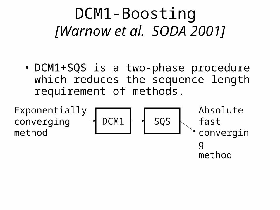
DCM1-Boosting [Warnow et al. SODA 2001]

• DCM1+SQS is a two-phase procedure which reduces the sequence length requirement of methods.

DCM1 SQSExponentiallyconvergingmethod

Absolute fast convergingmethod

Improving upon NJ

• Construct trees on a number of smaller diameter subproblems, and merge the subtrees into a tree on the full dataset.

• Our approach: – Phase I: produce O(n2) trees (one for each

diameter) – Phase II: pick the “best” tree from the set.

DCM1 Decompositions

DCM1 decomposition : Compute maximal cliques

Input: Set S of sequences, distance matrix d, threshold value

1. Compute threshold graph }),(:),{(,),,( qjidjiESVEVGq ≤===

2. Perform minimum weight triangulation (note: if d is an additive matrix, then the threshold graph is provably chordal).

}{ ijdq∈

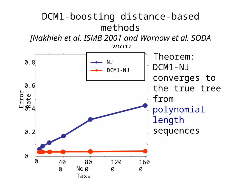
DCM1-boosting distance-based methods[Nakhleh et al. ISMB 2001 and Warnow et al. SODA 2001]

•Theorem: DCM1-NJ converges to the true tree from polynomial length sequences

NJ

DCM1-NJ

0 400 800 16001200No. Taxa

0

0.2

0.4

0.6

0.8

Err

or R

ate

What about solving MP and ML?

• Maximum Parsimony (MP) and maximum likelihood (ML) are the major phylogeny estimation methods used by systematists.

Maximum Parsimony

• Input: Set S of n aligned sequences of length k

• Output: A phylogenetic tree T– leaf-labeled by sequences in S– additional sequences of length k labeling the

internal nodes of T

such that is minimized. ∑∈ )(),(

),(TEji

jiH

Maximum Parsimony: computational complexity

ACT

ACA

GTT

GTAACA GTA

1 2 1

MP score = 4

Finding the optimal MP tree is NP-hard

Optimal labeling can becomputed in linear time O(nk)

1. Hill-climbing heuristics (which can get stuck in local optima)2. Randomized algorithms for getting out of local optima3. Approximation algorithms for MP (based upon Steiner Tree

approximation algorithms).

Approaches for “solving” MP/ML

Phylogenetic trees

Cost

Global optimum

Local optimum

Problems with current techniques for MP

0

0.02

0.04

0.06

0.08

0.1

0.12

0.14

0.16

0.18

0.2

0 4 8 12 16 20 24

Hours

Average MP score above

optimal, shown as a percentage of

the optimal

Best methods are a combination of simulated annealing, divide-and-conquer and genetic algorithms, as implemented in the software package TNT. However, theydo not reach 0.01% of optimal on large datasets in 24 hours.

Performance of TNT with time

Observations

• The best MP heuristics cannot get acceptably good solutions within 24 hours on most of these large datasets.

• Datasets of these sizes may need months (or years) of further analysis to reach reasonable solutions.

• Apparent convergence can be misleading.

How can we improve upon existing techniques?

Our objective: speed up the best MP heuristics

Time

MP scoreof best trees

Performance of hill-climbing heuristic

Desired Performance

Fake study

DCM Decompositions

DCM1 decomposition : Max cliques

DCM2 decomposition:Separator plus components

Input: Set S of sequences, distance matrix d, threshold value

1. Compute threshold graph }),(:),{(,),,( qjidjiESVEVGq ≤===

2. Perform minimum weight triangulation

}{ ijdq∈

Empirical observation

• No DCM based upon the threshold graphs gave us an improvement over the best heuristics for MP!

How can we improve upon existing techniques?

A conjecture as to why current techniques are poor:

• Our studies suggest that trees with near optimal scores tend to be topologically close (RF distance less than 15%) from the other near optimal trees.

• The best heuristics for MP are based upon the TBR move to explore tree space: there are O(n3) neighbors of every tree, most of which have large RF distances.

• So TBR may be useful initially (to reach near optimality) but then more “localized” searches are more productive.

Using DCMs differently

• Observation: DCMs make small local changes to the tree

• New algorithmic strategy: use DCMs iteratively and/or recursively to improve heuristics on large datasets

• We needed a decomposition strategy that produces small subproblems quickly.

New DCM3 decomposition

Input: Set S of sequences, and guide-tree T

1. We use a new graph (“short subtree graph”) G(S,T)) Note: G(S,T) is chordal!

2. Find clique separator in G(S,T) and form subproblems

DCM3 decompositions (1) can be obtained in O(n) time(2) yield small subproblems(3) can be used iteratively

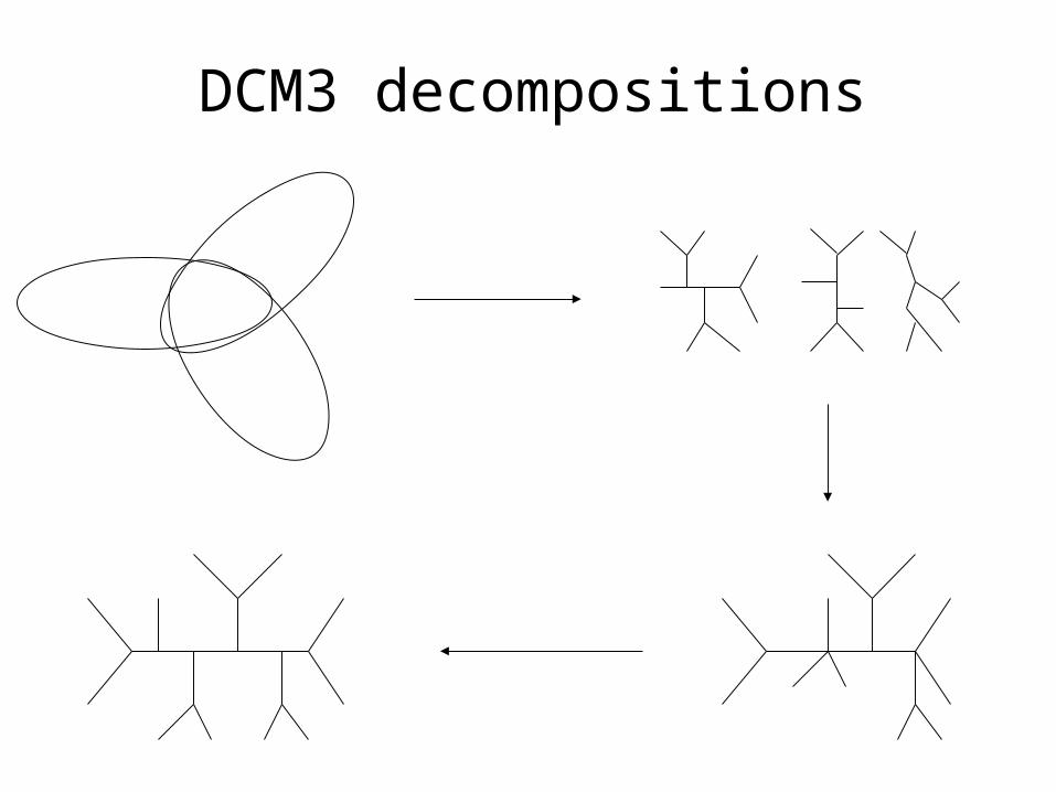
DCM3 decompositions

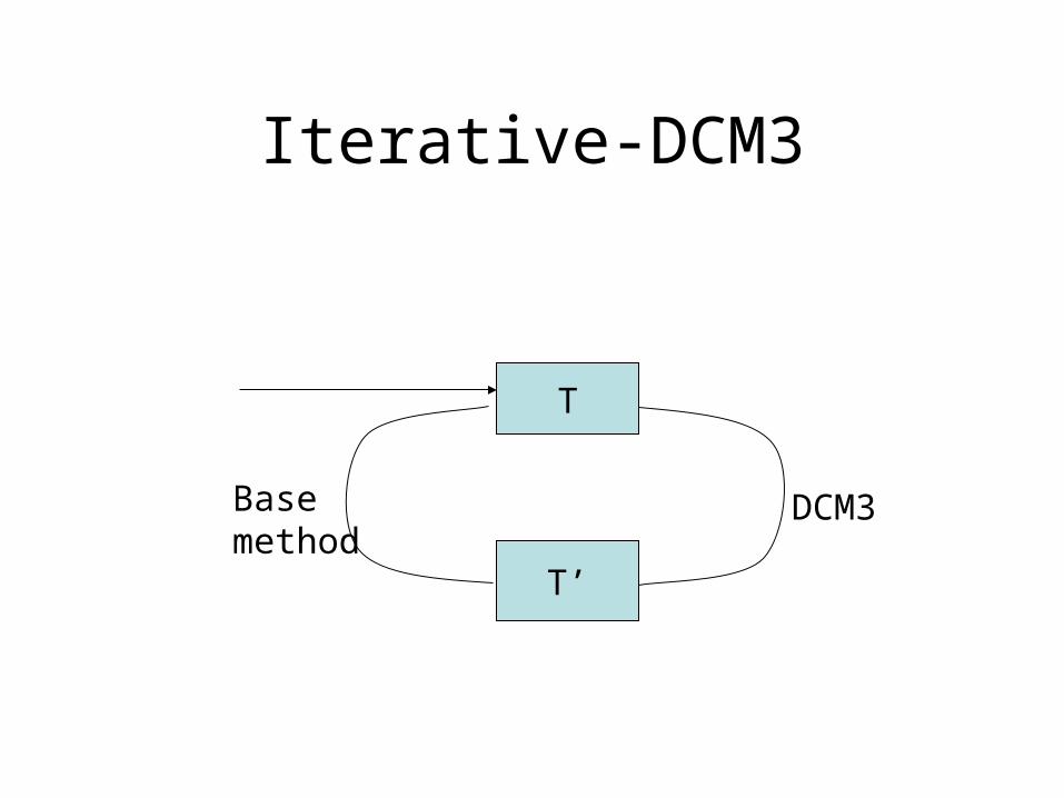
Iterative-DCM3

T

T’

DCM3Base method

Comparison of DCMs (13,921 sequences)

Base method is the TNT-ratchet. “Optimal” refers to the best score found by any method using any amount of time, to date.

0

0.05

0.1

0.15

0.2

0.25

0.3

0.35

0.4

0 4 8 12 16 20 24

Hours

Average MP score above

optimal, shown as a percentage of

the optimal

TNT DCM3 Rec-DCM3 I-DCM3 Rec-I-DCM3

Rec-I-DCM3 significantly improves performance

Comparison of TNT to Rec-I-DCM3(TNT) on one large dataset

0

0.02

0.04

0.06

0.08

0.1

0.12

0.14

0.16

0.18

0.2

0 4 8 12 16 20 24

Hours

Average MP score above

optimal, shown as a percentage of

the optimal

Current best techniques

DCM boosted version of best techniques

Conclusions (and comments)

• Rec-I-DCM3 improves upon the best performing heuristics for MP.

• The improvement increases with the difficulty of the dataset.

• DCMs also boost the performance of ML heuristics (not shown).

• Rec-I-DCM3 will be in the first software release from the CIPRES project

Other research projects

• Simultaneous estimation of tree and multiple sequence alignment

• Supertree methods• Constructing networks rather than trees (detecting

and reconstructing reticulate evolution)• Obtaining better bounds on sequence length

requirements of phylogeny reconstruction methods• Whole genome phylogeny• Constructing forests rather than trees

Acknowledgments

• The CIPRES project www.phylo.org• The National Science Foundation• The David and Lucile Packard Foundation• The Program for Evolutionary Dynamics at

Harvard, and the Radcliffe Institute for Advanced Research

• The Institute for Cellular and Molecular Biology at UT-Austin

• Collaborators: Bernard Moret, Usman Roshan, Tiffani Williams, and Daniel Huson.