Christopher Dougherty EC220 - Introduction to econometrics (chapter 4) Slideshow: elasticities and...

Christopher Dougherty

EC220 - Introduction to econometrics (chapter 4)Slideshow: elasticities and logarithmic models

Original citation:

Dougherty, C. (2012) EC220 - Introduction to econometrics (chapter 4). [Teaching Resource]

© 2012 The Author

This version available at: http://learningresources.lse.ac.uk/130/

Available in LSE Learning Resources Online: May 2012

This work is licensed under a Creative Commons Attribution-ShareAlike 3.0 License. This license allows the user to remix, tweak, and build upon the work even for commercial purposes, as long as the user credits the author and licenses their new creations under the identical terms. http://creativecommons.org/licenses/by-sa/3.0/

http://learningresources.lse.ac.uk/

http://learningresources.lse.ac.uk/

http://creativecommons.org/licenses/by-sa/3.0/

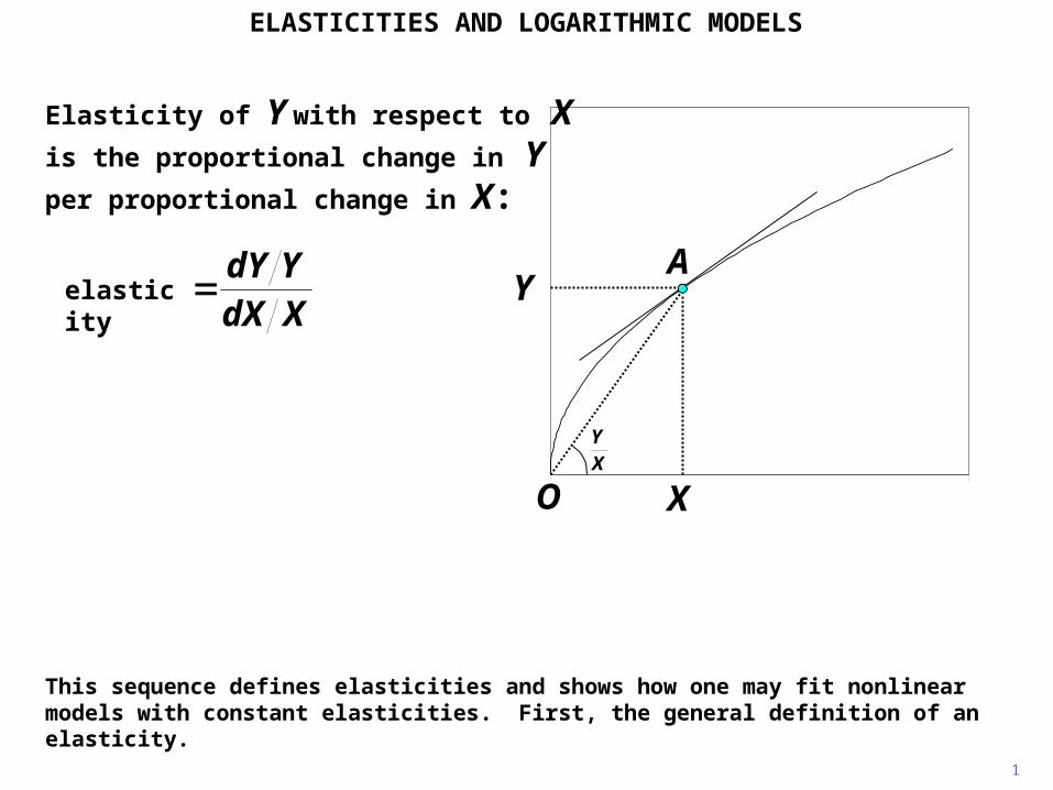
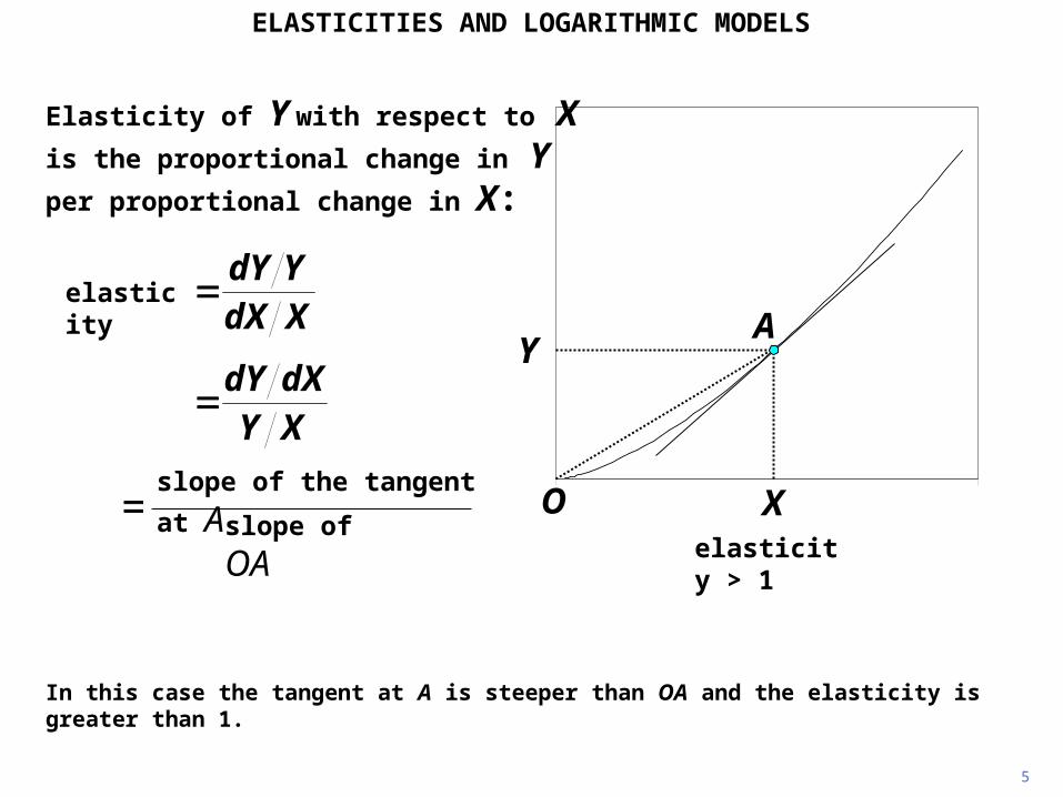
Elasticity of Y with respect to Xis the proportional change in Yper proportional change in X:

ELASTICITIES AND LOGARITHMIC MODELS

0 52

Y

X

A

O

1

This sequence defines elasticities and shows how one may fit nonlinear models with constant elasticities. First, the general definition of an elasticity.

XYXY

dXdY

XdXYdY

elasticity

XYdXdY

XdXYdY

Y

X

A

2

Re-arranging the expression for the elasticity, we can obtain a graphical interpretation.

0 52

XY

O



elasticity

slope of the tangent at Aslope of OA

Y

X

A

3

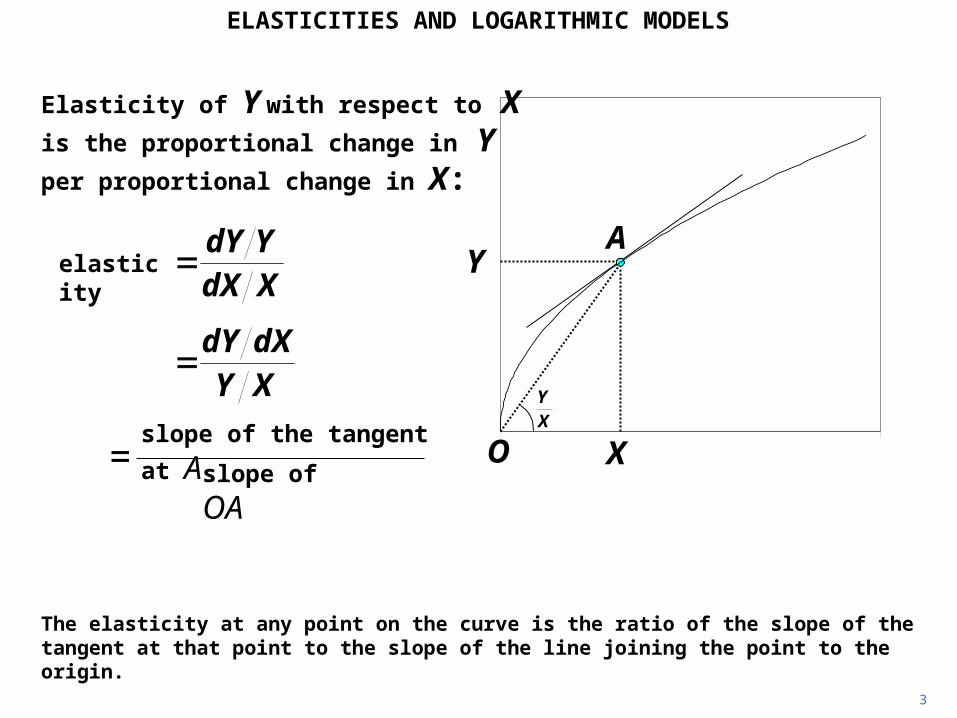
The elasticity at any point on the curve is the ratio of the slope of the tangent at that point to the slope of the line joining the point to the origin.

0 52

XY

O



XYdXdY

XdXYdY

elasticity


4

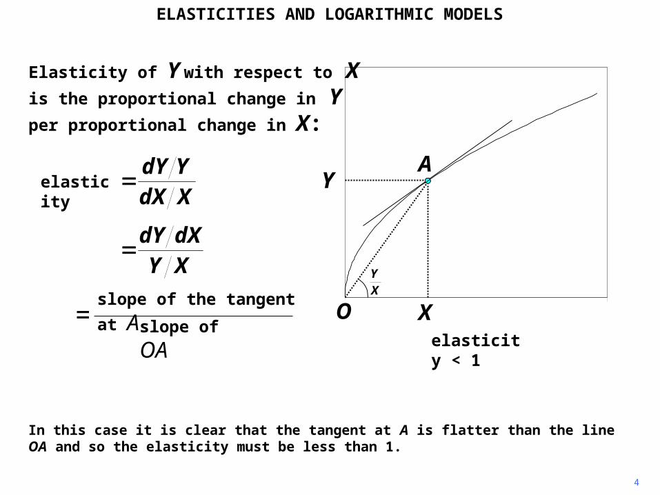
In this case it is clear that the tangent at A is flatter than the line OA and so the elasticity must be less than 1.

Y

X

A

XY

0 52O



XYdXdY

XdXYdY

elasticity

slope of the tangent at Aslope of OA elasticity < 1

0 52

5

In this case the tangent at A is steeper than OA and the elasticity is greater than 1.

A

O

Y

X



XYdXdY

XdXYdY

elasticity

slope of the tangent at Aslope of OA elasticity > 1

6

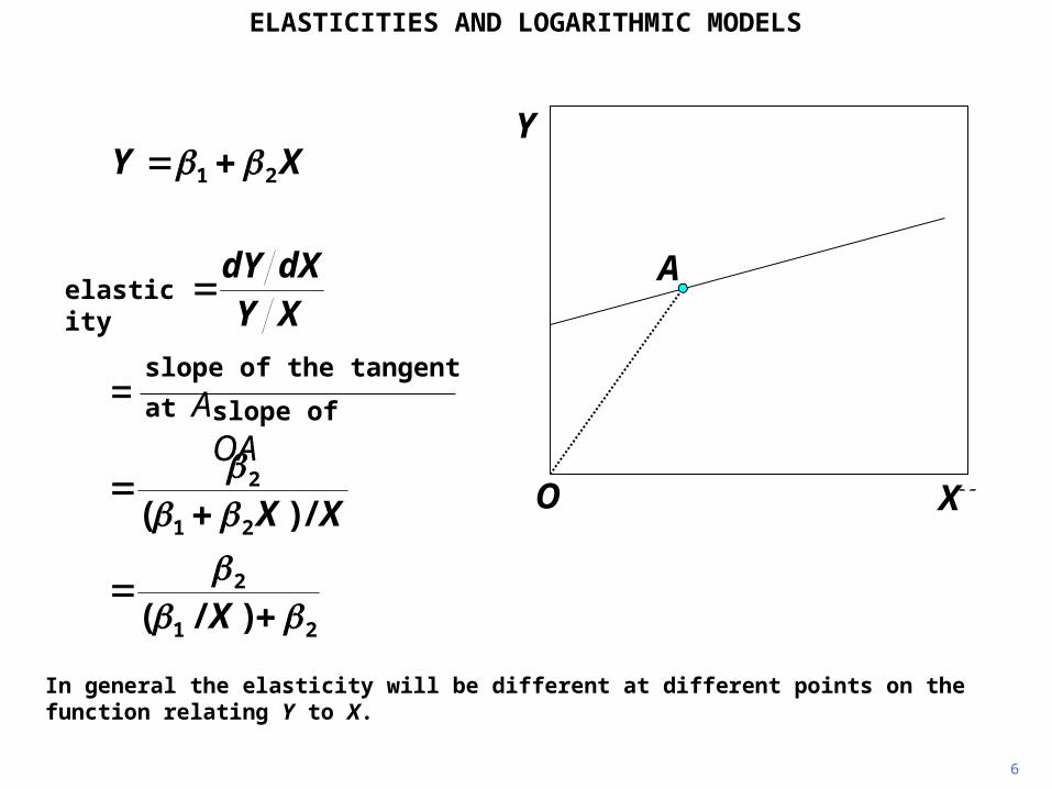
In general the elasticity will be different at different points on the function relating Y to X.

Y

xO X

XY 21

21

2

21

2

)/(

/)(

X

XX

A



XYdXdY

elasticity

7

In the example above, Y is a linear function of X.

xO

A

XY 21 Y

X


21

2

21

2

)/(

/)(

X

XX


XYdXdY

elasticity

8

The tangent at any point is coincidental with the line itself, so in this case its slope is always 2. The elasticity depends on the slope of the line joining the point to the origin.

xO

A

XY 21 Y

X


21

2

21

2

)/(

/)(

X

XX


XYdXdY

elasticity

9

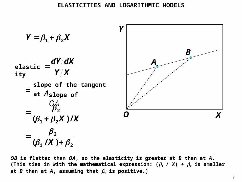
OB is flatter than OA, so the elasticity is greater at B than at A. (This ties in with the mathematical expression: (1/ X) + 2 is smaller at B than at A, assuming that 1 is positive.)

x

A

O

B

XY 21 Y

X


21

2

21

2

)/(

/)(

X

XX


XYdXdY

elasticity

21

XY

10

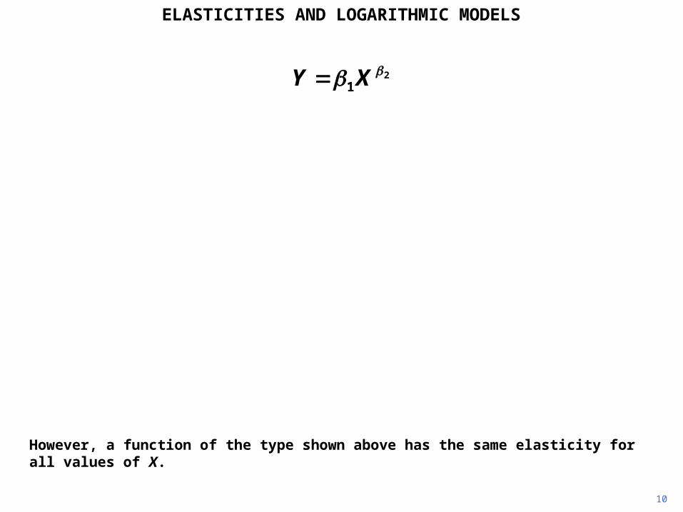
However, a function of the type shown above has the same elasticity for all values of X.


21

XY

121

2 XdXdY

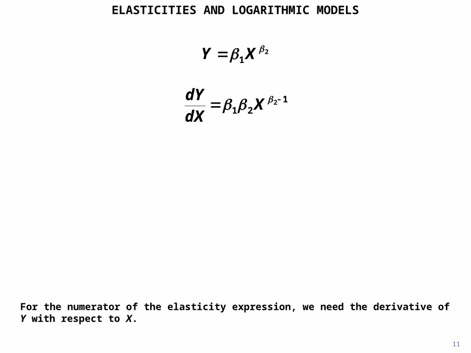
11

For the numerator of the elasticity expression, we need the derivative of Y with respect to X.


21

XY

121

2 XdXdY

11

1 2

2

X

XX

XY

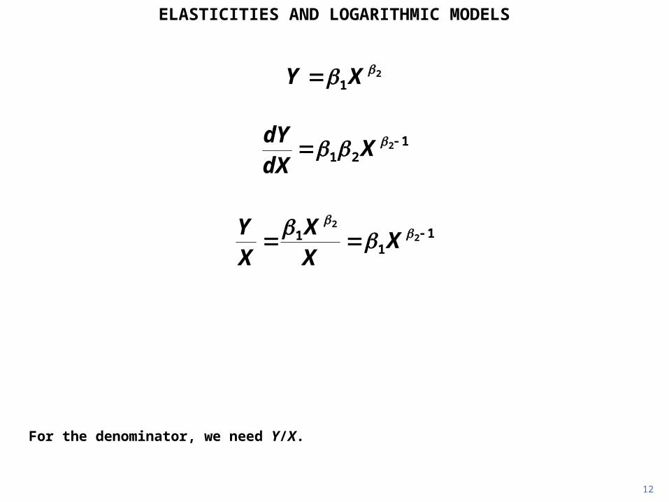
12

For the denominator, we need Y/X.


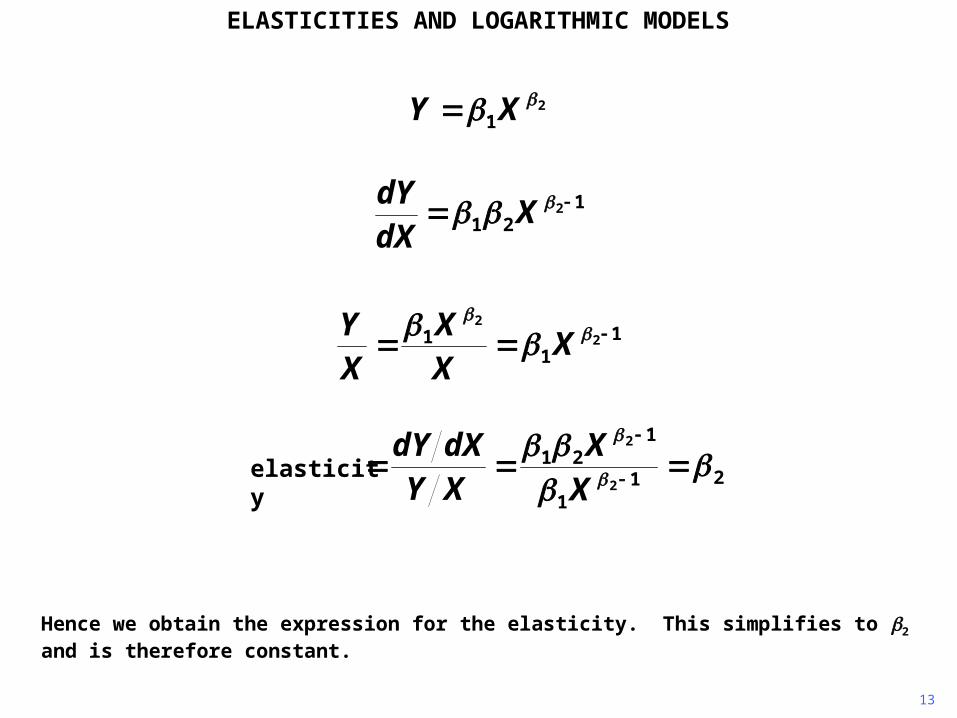
13

Hence we obtain the expression for the elasticity. This simplifies to 2 and is therefore constant.

21

XY

121

2 XdXdY

11

1 2

2

X

XX

XY


elasticity 211

121

2

2

X

XXYdXdY

14

By way of illustration, the function will be plotted for a range of values of 2. We will start with a very low value, 0.25.

Y

X

21

XY 25.02


15

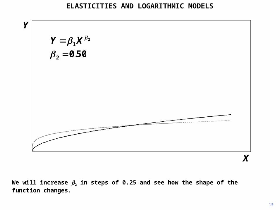
We will increase 2 in steps of 0.25 and see how the shape of the function changes.

21

XY 50.02

Y

X


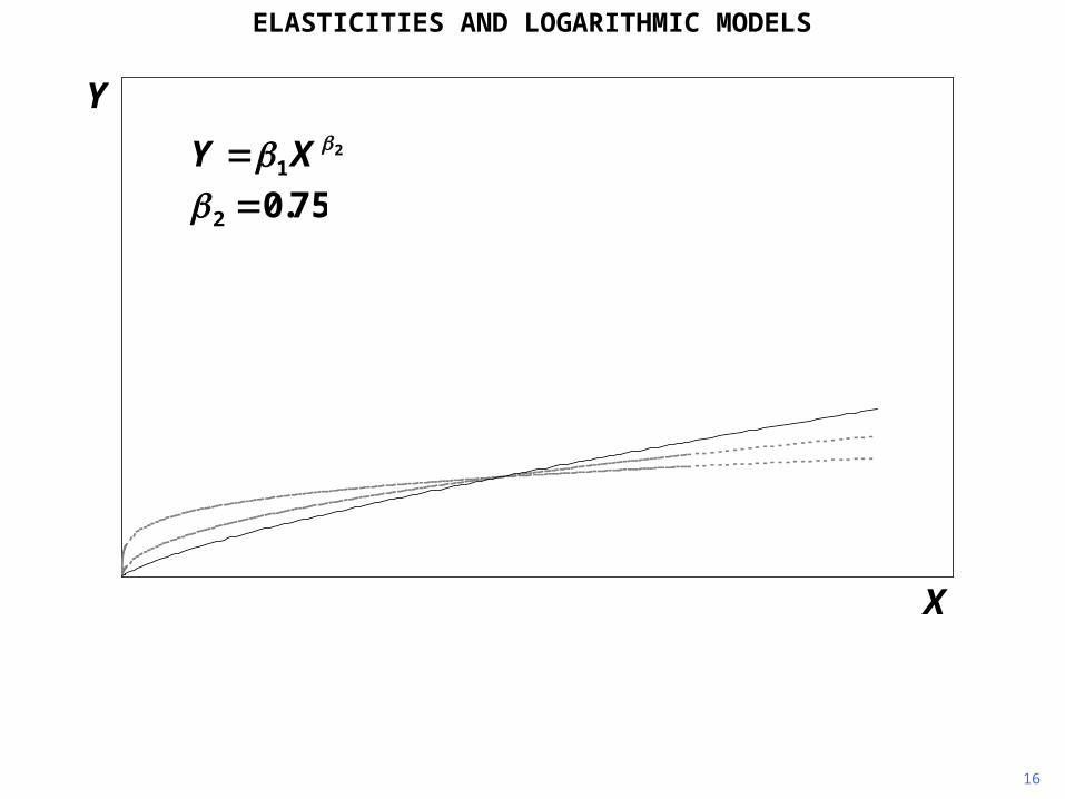
16

21

XY 75.02

Y

X


17

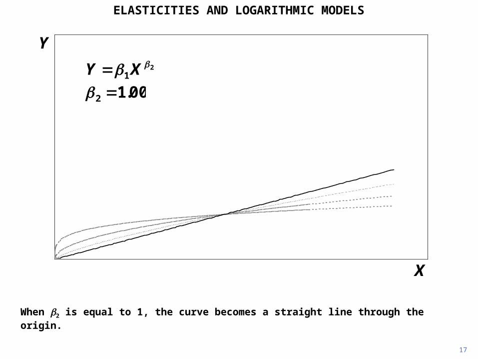
When 2 is equal to 1, the curve becomes a straight line through the origin.

21

XY 00.12

Y

X


18

21

XY 25.12

Y

X


19

21

XY 50.12

Y

X


20

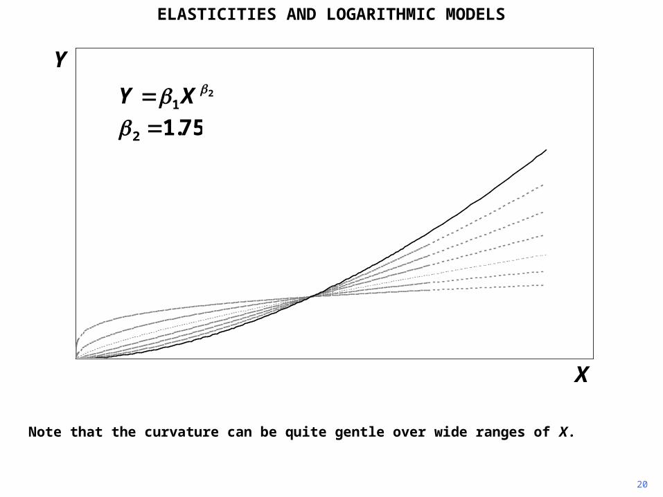
Note that the curvature can be quite gentle over wide ranges of X.

21

XY 75.12

Y

X


21

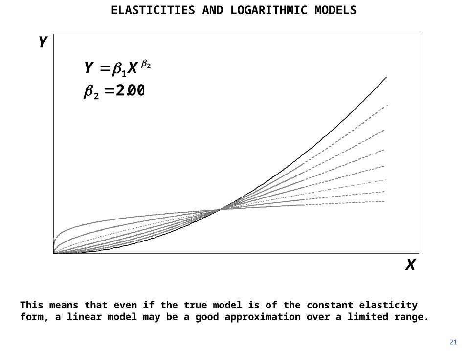
This means that even if the true model is of the constant elasticity form, a linear model may be a good approximation over a limited range.

21

XY 00.22

Y

X


22

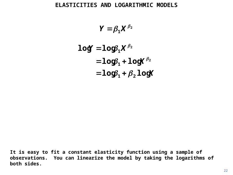
It is easy to fit a constant elasticity function using a sample of observations. You can linearize the model by taking the logarithms of both sides.

21

XY

X

X

XY

loglog

loglog

loglog

21

1

1

2

2


23

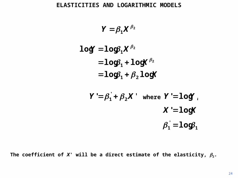
You thus obtain a linear relationship between Y' and X', as defined. All serious regression applications allow you to generate logarithmic variables from existing ones.

21

XY

X

X

XY

loglog

loglog

loglog

21

1

1

2

2

'' 2'1 XY


1'1 log

log'

,log'

XX

YYwhere

24

The coefficient of X' will be a direct estimate of the elasticity, 2.

21

XY

X

X

XY

loglog

loglog

loglog

21

1

1

2

2


'' 2'1 XY

1'1 log

log'

,log'

XX

YYwhere

25

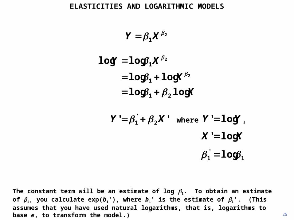
The constant term will be an estimate of log 1. To obtain an estimate of 1, you calculate exp(b1'), where b1' is the estimate of 1'. (This assumes that you have used natural logarithms, that is, logarithms to base e, to transform the model.)

21

XY

X

X

XY

loglog

loglog

loglog

21

1

1

2

2


'' 2'1 XY

1'1 log

log'

,log'

XX

YYwhere

26

Here is a scatter diagram showing annual household expenditure on FDHO, food eaten at home, and EXP, total annual household expenditure, both measured in dollars, for 1995 for a sample of 869 households in the United States (Consumer Expenditure Survey data).

0

2000

4000

6000

8000

10000

12000

14000

16000

0 20000 40000 60000 80000 100000 120000 140000 160000

FDHO

EXP


. reg FDHO EXP

Source | SS df MS Number of obs = 869---------+------------------------------ F( 1, 867) = 381.47 Model | 915843574 1 915843574 Prob > F = 0.0000Residual | 2.0815e+09 867 2400831.16 R-squared = 0.3055---------+------------------------------ Adj R-squared = 0.3047 Total | 2.9974e+09 868 3453184.55 Root MSE = 1549.5

------------------------------------------------------------------------------ FDHO | Coef. Std. Err. t P>|t| [95% Conf. Interval]---------+-------------------------------------------------------------------- EXP | .0528427 .0027055 19.531 0.000 .0475325 .0581529 _cons | 1916.143 96.54591 19.847 0.000 1726.652 2105.634------------------------------------------------------------------------------

27

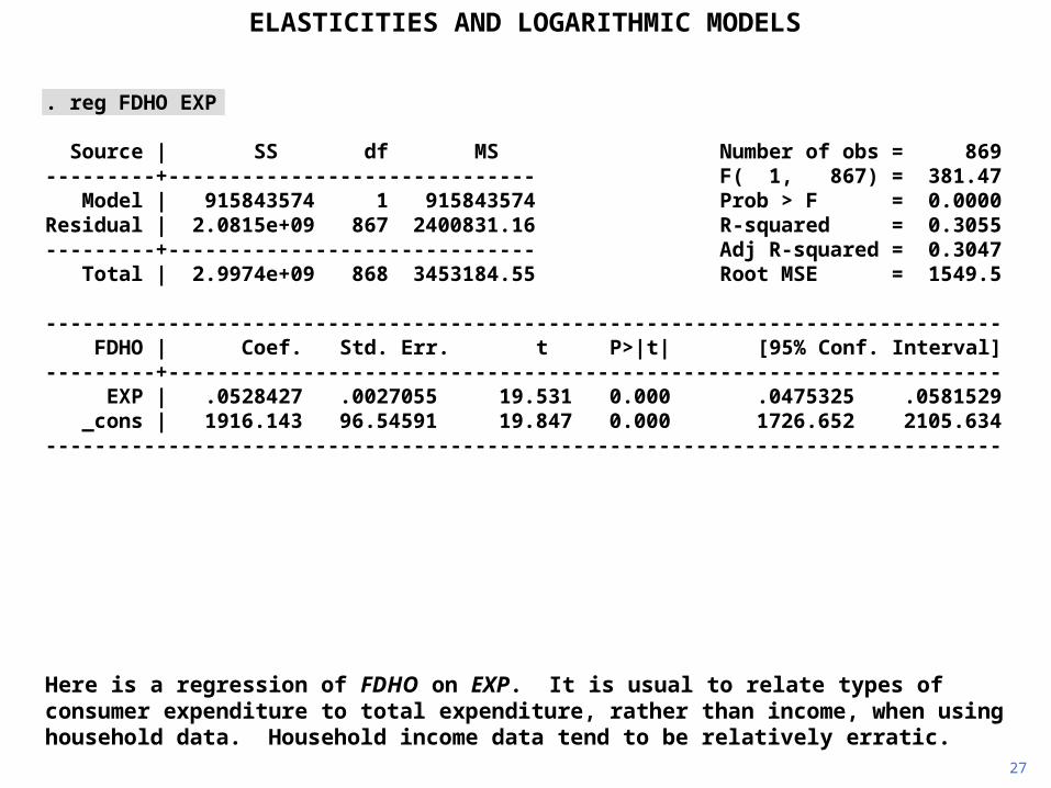
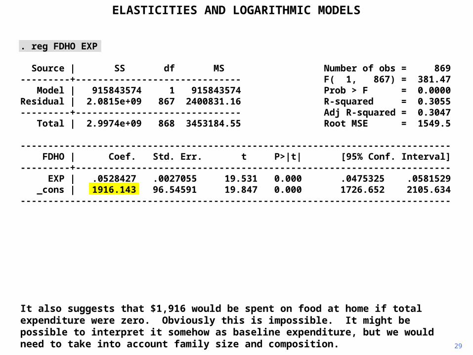
Here is a regression of FDHO on EXP. It is usual to relate types of consumer expenditure to total expenditure, rather than income, when using household data. Household income data tend to be relatively erratic.


. reg FDHO EXP



28

The regression implies that, at the margin, 5 cents out of each dollar of expenditure is spent on food at home. Does this seem plausible? Probably, though possibly a little low.


. reg FDHO EXP



29

It also suggests that $1,916 would be spent on food at home if total expenditure were zero. Obviously this is impossible. It might be possible to interpret it somehow as baseline expenditure, but we would need to take into account family size and composition.


30

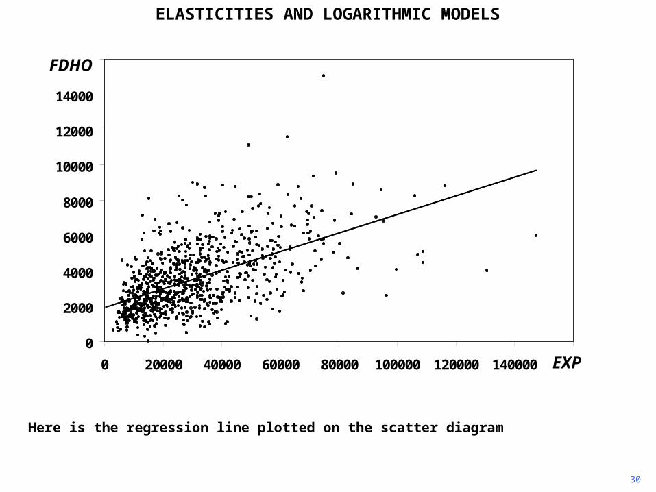
Here is the regression line plotted on the scatter diagram

0

2000

4000

6000

8000

10000

12000

14000

16000

0 20000 40000 60000 80000 100000 120000 140000 160000EXP

FDHO


31

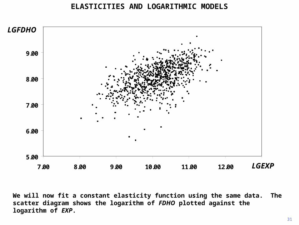
We will now fit a constant elasticity function using the same data. The scatter diagram shows the logarithm of FDHO plotted against the logarithm of EXP.

5.00

6.00

7.00

8.00

9.00

10.00

7.00 8.00 9.00 10.00 11.00 12.00 13.00

LGFDHO

LGEXP


. g LGFDHO = ln(FDHO)

. g LGEXP = ln(EXP)

. reg LGFDHO LGEXP

Source | SS df MS Number of obs = 868---------+------------------------------ F( 1, 866) = 396.06 Model | 84.4161692 1 84.4161692 Prob > F = 0.0000Residual | 184.579612 866 .213140429 R-squared = 0.3138---------+------------------------------ Adj R-squared = 0.3130 Total | 268.995781 867 .310260416 Root MSE = .46167

------------------------------------------------------------------------------ LGFDHO | Coef. Std. Err. t P>|t| [95% Conf. Interval]---------+-------------------------------------------------------------------- LGEXP | .4800417 .0241212 19.901 0.000 .4326988 .5273846 _cons | 3.166271 .244297 12.961 0.000 2.686787 3.645754------------------------------------------------------------------------------

32

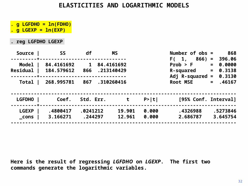
Here is the result of regressing LGFDHO on LGEXP. The first two commands generate the logarithmic variables.



. g LGEXP = ln(EXP)

. reg LGFDHO LGEXP



33

The estimate of the elasticity is 0.48. Does this seem plausible?



. g LGEXP = ln(EXP)

. reg LGFDHO LGEXP



34

Yes, definitely. Food is a normal good, so its elasticity should be positive, but it is a basic necessity. Expenditure on it should grow less rapidly than expenditure generally, so its elasticity should be less than 1.



. g LGEXP = ln(EXP)

. reg LGFDHO LGEXP



35

The intercept has no substantive meaning. To obtain an estimate of 1, we calculate e3.16, which is 23.8.

48.08.23ˆ48.017.3ˆ EXPOHFDLGEXPHODLGF


36

Here is the scatter diagram with the regression line plotted.

5.00

6.00

7.00

8.00

9.00

10.00

7.00 8.00 9.00 10.00 11.00 12.00 13.00

LGFDHO

LGEXP


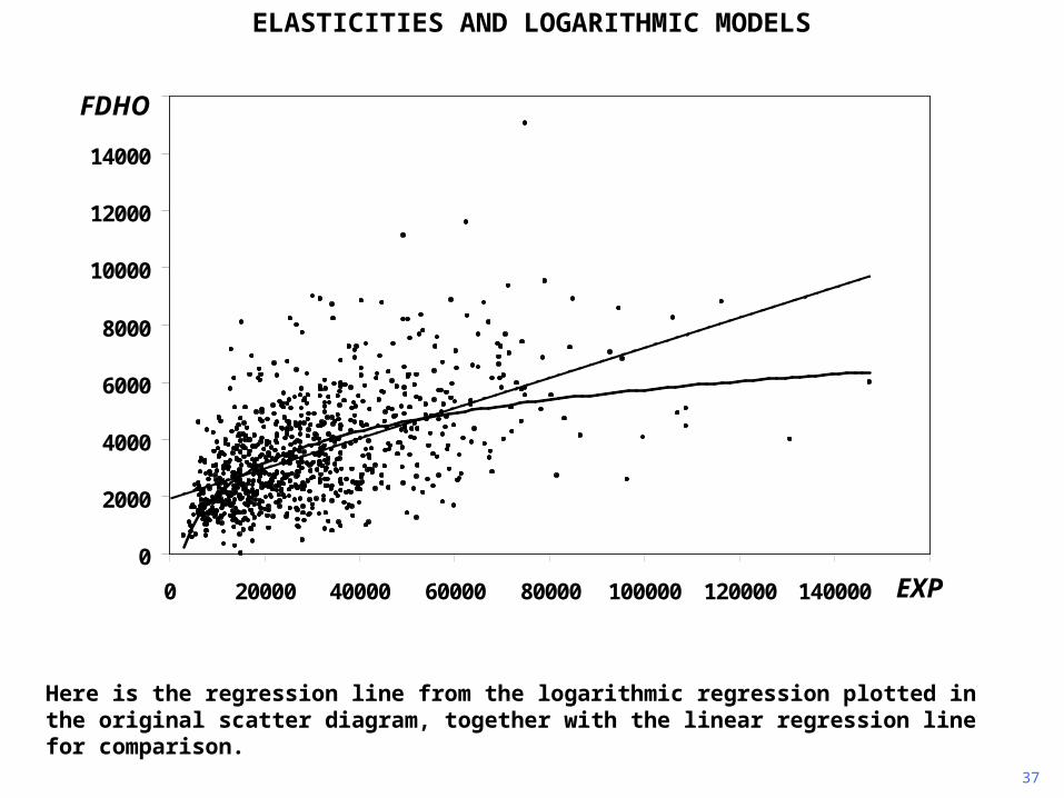
37

Here is the regression line from the logarithmic regression plotted in the original scatter diagram, together with the linear regression line for comparison.

0

2000

4000

6000

8000

10000

12000

14000

16000

0 20000 40000 60000 80000 100000 120000 140000 160000EXP

FDHO


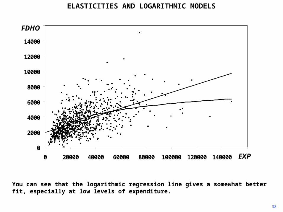
38

You can see that the logarithmic regression line gives a somewhat better fit, especially at low levels of expenditure.

0

2000

4000

6000

8000

10000

12000

14000

16000

0 20000 40000 60000 80000 100000 120000 140000 160000EXP

FDHO


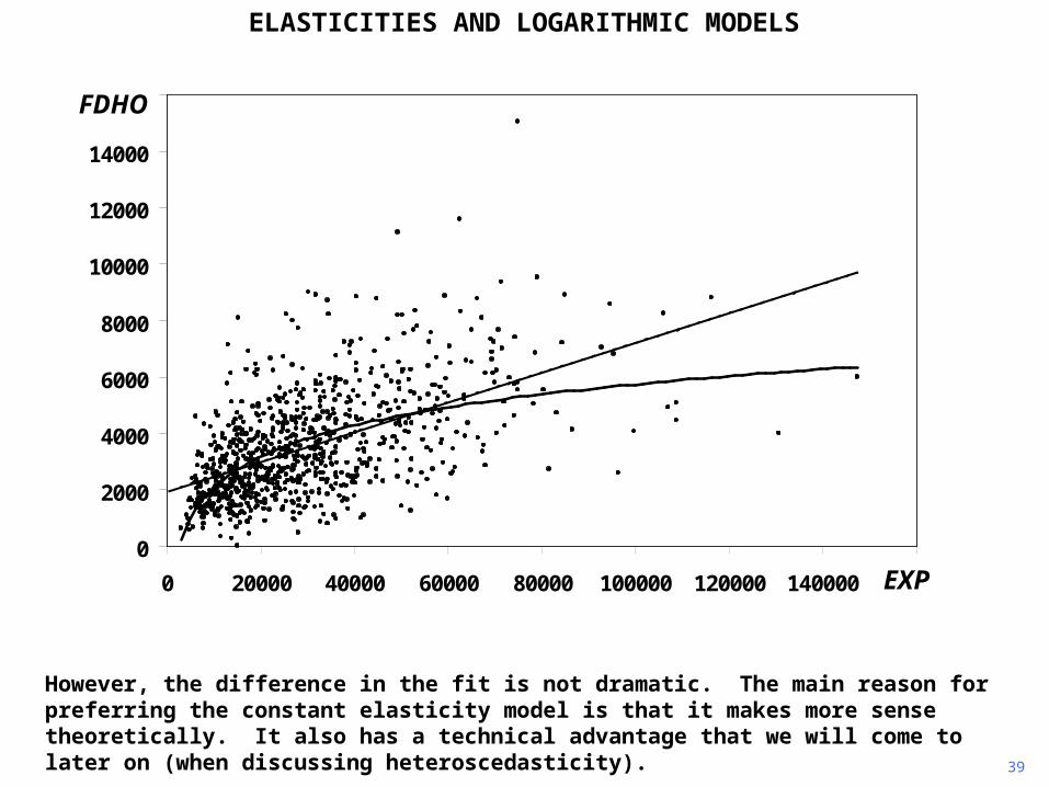
39

However, the difference in the fit is not dramatic. The main reason for preferring the constant elasticity model is that it makes more sense theoretically. It also has a technical advantage that we will come to later on (when discussing heteroscedasticity).

0

2000

4000

6000

8000

10000

12000

14000

16000

0 20000 40000 60000 80000 100000 120000 140000 160000EXP

FDHO


Copyright Christopher Dougherty 2011.

These slideshows may be downloaded by anyone, anywhere for personal use.

Subject to respect for copyright and, where appropriate, attribution, they may be

used as a resource for teaching an econometrics course. There is no need to

refer to the author.

The content of this slideshow comes from Section 4.2 of C. Dougherty,

Introduction to Econometrics, fourth edition 2011, Oxford University Press.

Additional (free) resources for both students and instructors may be

downloaded from the OUP Online Resource Centre

http://www.oup.com/uk/orc/bin/9780199567089/.

Individuals studying econometrics on their own and who feel that they might

benefit from participation in a formal course should consider the London School

of Economics summer school course

EC212 Introduction to Econometrics

http://www2.lse.ac.uk/study/summerSchools/summerSchool/Home.aspx

or the University of London International Programmes distance learning course

20 Elements of Econometrics

www.londoninternational.ac.uk/lse.

11.07.25

http://www.oup.com/uk/orc/bin/9780199567089/

http://www2.lse.ac.uk/study/summerSchools/summerSchool/Home.aspx

Christopher Dougherty EC220 - Introduction to econometrics (chapter 4) Slideshow: elasticities and...

Documents

Transcript of Christopher Dougherty EC220 - Introduction to econometrics (chapter 4) Slideshow: elasticities and...