An Investigation of Loudspeaker Simulation Efficiency and Accuracy using i) A Conventional Model, ii) The Near-To-Far-Field Transforma-tion and iii) The Rayleigh Integral Ulrik Skov*1 and René Christensen**1 1iCapture ApS Skomagergade 82th, DK-4000 Roskilde, Denmark *Corresponding author, us@iCapture.dk **Presenting author, rc@iCapture.dk Abstract: Simulation on loudspeaker drivers require a conventional fully coupled vibro-acoustic model to capture both the effect of the loading mass of the air on the moving parts and the geometric topology of the cone, dust cap and surround. An accurate vibroacoustic model can be time-consuming to solve, especially in 3D. In practical applications, this results in poor efficiency concerning the decision-making process to move on to the next simulation model. To overcome this the loudspeaker designer can use either the COMSOL build-in near-to-far-field transformation (PFAR) or post-process structural only results via the Rayleigh integral to reduce or totally eliminate the computationally demanding open air domain in front of the speaker. These simplifications comes with the cost of a frequency dependent inaccuracy. This paper compares for three different drivers (a totally flat, a concave cone and a convex dome) the efficiency and accuracy of a conventional fully coupled vibroacoustic model where the measurement point is included in the computational FEA domain with respectively a reduced air domain model having the measurement point outside the computational FEA domain obtained by the near-to-far-field transformation and a model relying on the structural only Rayleigh integral post-processing. Keywords: Near-to-far-field transformation, PFAR, Helmholtz-Kirchhoff and Rayleigh. 1. Introduction Simulation driven design and product development is becoming the development department’s new third leg complimenting the two classical legs of theory and measurements.

The past years many companies has successfully established vibroacoustic simulation capability to simulate axi-symmetric loudspeaker drivers in 2D.

Modelling all moving parts of a loudspeaker – such as the surround, cone, dust cap, former, reinforcement, windings, spider and the glue –

gives access to high fidelity and robust simulation results, which can be relied on during everyday decision making.

Such a fully coupled 2D linear vibroacoustic harmonic analysis takes few hours to setup and a matter of minutes to run producing few mega byte data. This makes the working method both efficient in the pre-processing, solving and post-processing phases.

However, if the physical driver cyclic periodic geometric features such as ribs in the surround, cone, dust cap, spider or back chamber a 2D axisymmetric model is no longer an option. The designer must either build and setup a cyclic periodic 3D-model using harmonic indexes or create a full 3D-model. Doing this the solving time increases to weeks and months – and post-processing starts to become significantly a time-vice burden due to the large amounts of generated data in the tera byte region. 3D modelling thereby is understood to have a poor efficiency in the pre-processing phase and an unacceptable efficiency in the solving and post-processing phases.

To overcome this limitation of 3D-modelling one can reduce the computational burden by reducing the open air domain to barely include the driver excluding the distant measurement point from the computational domain typically located between 0.4-1.0m distance from the driver. The radiated acoustic signal beyond the reduced air domain can be found by the near-to-far-field transformation allowing the calculation of the pressure field outside the computational FEA domain via the COMSOL build-in far field functionality, PFAR. This method is based on computing the full Helmhotz-Kirchoff integral resulting in similar accuracy as running a model with the entire open air domain. However the computational burden has decreased resulting in an increasing efficiency during solving and post-processing.

An alternative solution is to totally remove the open air domain in front of the driver and calculate on a structural only 3D-model. The

radiated acoustic signal is then found by post-processing via the Rayleigh-integral, which is a reduction of the Helmhotz-Kirchoff integral by use of a half-space Green’s function.

The Rayleigh integral introduced two types of errors concerning i) the geometric topology of the cone, dust cap and surround (i.e. the Rayleigh integral presumes the face of the driver to be totally flat) and ii) the fact that the mass of the air loading the cone, dust cap and surround is omitted.

For simplicity and pragmatic reasons, it was decided to do the work on 2D axisymmetric models, despite the gain in efficiency is much more significant for 3D cyclic periodic or full models. The objective of this paper is to investigate the accuracy and efficiency on three different drivers (totally flat, concave cone and convex dome) using:

i) a fully coupled vibroacoustic model including the measurement point in the computational FEA domain,

ii) COMSOL’s build-in near-to-far-field transformation (PFAR) on a fully coupled vibroacoustic model with reduced air domain having the measurement point outside the computational FEA domain and

iii) a structural only model using the Rayleigh integral.

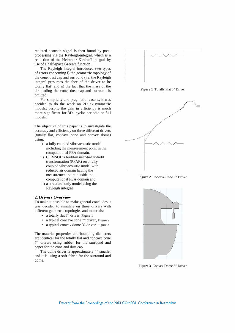
2. Drivers Overview To make it possible to make general concludes it was decided to simulate on three drivers with different geometric topologies and materials:

• a totally flat 7” driver, Figure 1 • a typical concave cone 7” driver, Figure 2 • a typical convex dome 3” driver, Figure 3

The material properties and bounding diameters are identical for the totally flat and concave cone 7” drivers using rubber for the surround and paper for the cone and dust cap.

The dome driver is approximately 4” smaller and it is using a soft fabric for the surround and dome.

Figure 1 Totally Flat 6” Driver

Figure 2 Concave Cone 6” Driver

Figure 3 Convex Dome 3” Driver

3. Modelling Strategy The modelling strategy was to place the drivers in a half-space baffle and take account of all geometric features including the glue to base the work on high fidelity models. Thereby it is understood that none of the models suffers from inaccuracies related to mathematical linking of the finite elements (so called “pin joints”) between different parts such as the attachment of the cone or spider to the voice coil [1]. 4. Methods This section briefly give the overview of the three methods used to extract the acoustic pressure responses. 4.1 Fully coupled incl. measurement point A fully coupled model is a vibroacoustic model consisting of both structural and acoustic domains having the measurement point included in the computational FEA domain.

Typically, the physical measurement is located 1m in front of the driver.

For this work it was decided only to include 0.5mi air and simulate the sound pressure level in a distance of 0.4m.

The upside of using a fully coupled model is that all behaviour is captured in both the structural and acoustic domains. I.e. both near- and far-field acoustics and structural displacements and stresses can be illustrated and animated.

The downside is the computational burden. 4.2 Fully coupled excl. point using PFAR A model using the COMSOL near-to-far-field transformation (PFAR) is identical to the model described in section 3.1, but with a reduced air domain only encapsulating the structure excluding the measurement point in the computational FEA domain. For this work the reduced air domain is 0.08m and the simulated sound pressure level is calculated by the COMSOL build-in full Helmholtz-Kirchhoff integral [2]:

( )1,)(

)()()()()( ∫

∂∂+=

S

n dSn

rGQprGQviPpPC ρω

where: • P indicates an observation point, • Q is a point on the closed surface S

• )(PC is the spatial angle in the

measurement point, here π4 • ρ is the density of the medium

• )(Qvn is the normal velocity in point

Q with the normal denoted n , and

• the full space Green’s function is defined:

r

erG

ikr−

=)( , where

• r is the distance between points P and Q .

The upside of using a reduced fully coupled model using PFAR is that all behaviour is captured in the acoustic near-field and structural domains. I.e. only near-field acoustics and structural displacements and stresses can be illustrated and animated. Polar plots of directivity in the far-field can be illustrated.

The downside is a still significant however reduce computational burden compared with the full vibroacoustic model encapsulating the measurement point. 4.3 Structural only using Rayleigh A model using the Rayleigh integral is a structural only model having the measurement point also excluded in the computational FEA domain.

For this work the simulated sound pressure level is found by use of iCapture’s novel proprietary FEA2SCN program and Klippels scanning software [3].

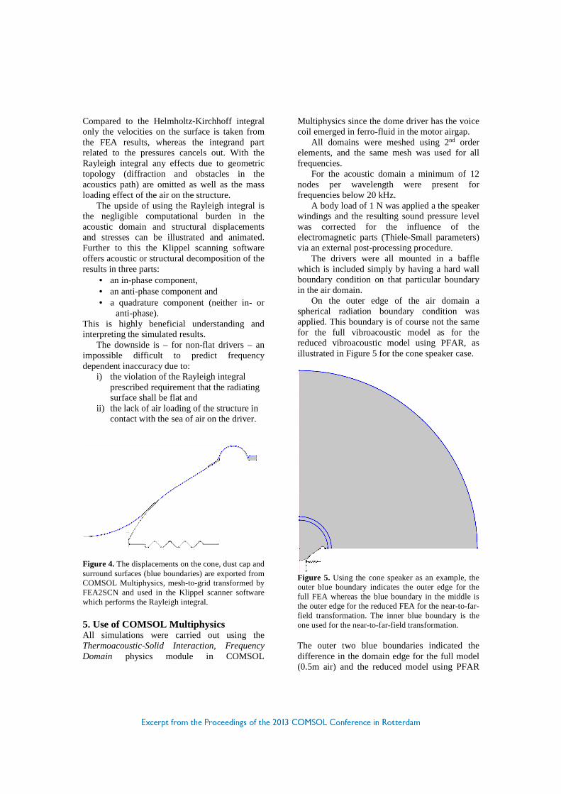
The FEA2SCN program transform the displacements of the unstructured FEA-mesh on the fluid structure interface i.e. the surface of the driver touching the sea of air to a structured scanner-grid, which is imported to Klippels scanning software where the Rayligh post-processing takes place. In Figure 4 the boundaries for which the displacements are exported are illustrated for the cone speaker case.

The Rayleigh integral equation can be found by considering the special case of a flat structure mounted in an acoustic “infinite” baffle. Using a half-space Green’s function, the Helmholtz-Kirchhoff integral equation reduces to the Rayleigh integral [2,4]:

( )2.)(2

)()( ∫=

S

n dSrGQvi

Ppπ

ρω

Compared to the Helmholtz-Kirchhoff integral only the velocities on the surface is taken from the FEA results, whereas the integrand part related to the pressures cancels out. With the Rayleigh integral any effects due to geometric topology (diffraction and obstacles in the acoustics path) are omitted as well as the mass loading effect of the air on the structure. The upside of using the Rayleigh integral is the negligible computational burden in the acoustic domain and structural displacements and stresses can be illustrated and animated. Further to this the Klippel scanning software offers acoustic or structural decomposition of the results in three parts:

• an in-phase component, • an anti-phase component and • a quadrature component (neither in- or

anti-phase). This is highly beneficial understanding and interpreting the simulated results. The downside is – for non-flat drivers – an impossible difficult to predict frequency dependent inaccuracy due to:

i) the violation of the Rayleigh integral prescribed requirement that the radiating surface shall be flat and

ii) the lack of air loading of the structure in contact with the sea of air on the driver.

Figure 4. The displacements on the cone, dust cap and surround surfaces (blue boundaries) are exported from COMSOL Multiphysics, mesh-to-grid transformed by FEA2SCN and used in the Klippel scanner software which performs the Rayleigh integral.

5. Use of COMSOL Multiphysics All simulations were carried out using the Thermoacoustic-Solid Interaction, Frequency Domain physics module in COMSOL

Multiphysics since the dome driver has the voice coil emerged in ferro-fluid in the motor airgap.

All domains were meshed using 2nd order elements, and the same mesh was used for all frequencies.

For the acoustic domain a minimum of 12 nodes per wavelength were present for frequencies below 20 kHz.

A body load of 1 N was applied a the speaker windings and the resulting sound pressure level was corrected for the influence of the electromagnetic parts (Thiele-Small parameters) via an external post-processing procedure.

The drivers were all mounted in a baffle which is included simply by having a hard wall boundary condition on that particular boundary in the air domain.

On the outer edge of the air domain a spherical radiation boundary condition was applied. This boundary is of course not the same for the full vibroacoustic model as for the reduced vibroacoustic model using PFAR, as illustrated in Figure 5 for the cone speaker case.

Figure 5. Using the cone speaker as an example, the outer blue boundary indicates the outer edge for the full FEA whereas the blue boundary in the middle is the outer edge for the reduced FEA for the near-to-far-field transformation. The inner blue boundary is the one used for the near-to-far-field transformation. The outer two blue boundaries indicated the difference in the domain edge for the full model (0.5m air) and the reduced model using PFAR

(0.08m air), respectively. The inner blue boundary indicates the surface used in the near-to-far-field transformation, see section 3.2. In COMSOL Multiphysics the functionality is called Far-Field Calculation. The surface in question is selected, and a symmetry condition is applied emulating the baffle. 6. Results This section describes and compare the results from the three drivers.

6.1 Absolute Sound Pressure Levels The Rayleigh integral will be applied both on a driver loaded with air (the fully coupled model) and a structural only model to show the effect of the mass of the air loading the cone, dust cap and surround. This results in four curves for each driver:

• Vibroacoustic (0.5m air). • Vibroacoustic (0.5m air) using Rayleigh. • Vibroacoustic (0.08m) using PFAR. • Structural only (no air) using Rayleigh.

Note that the curve “Vibroacoustic (0.5m) using Rayleigh)” is found on the exact same model used to make the curve “Vibroacoustic (0.5m)”.

The four curves for each driver are seen in Figure 6 and discussed in section 7. 6.2 Differences Sound Pressure Levels Based on these results the following four comparisons can be investigated for each driver:

• PFAR inaccuracy is identified via a fully coupled model with the measurement point included in the computational FEA domain “Vibroacoustic (0.5m air)” and a reduced air domain model with the measurement point outside the computational FEA domain using the COMSOL near-to-far- field transformation “Vibroacoustic (0.08m) using PFAR”.

• Rayleigh geometric topology inaccuracy is identified via a fully coupled model with the measurement point included in the computational FEA domain “Vibroacoustic (0.5m air)” and a vibroacoustic model using Rayleigh “Vibroacoustic (0.5m air) using Rayleigh”.

• Rayleigh mass of air loading inaccuracy is identified via a fully

coupled model using Rayleigh “Vibroacoustic (0.5m air) using Rayleigh” and a structural only model using Rayleigh “Structural only (no air) using Rayleigh”.

• Rayleigh total (geometry and mass of air) inaccuracy is identified via a fully coupled model with the measurement point included in the computational FEA domain “Vibroacoustic (0.5m air)” and a structural only model using Rayleigh “Structural only (no air) using Rayleigh”.

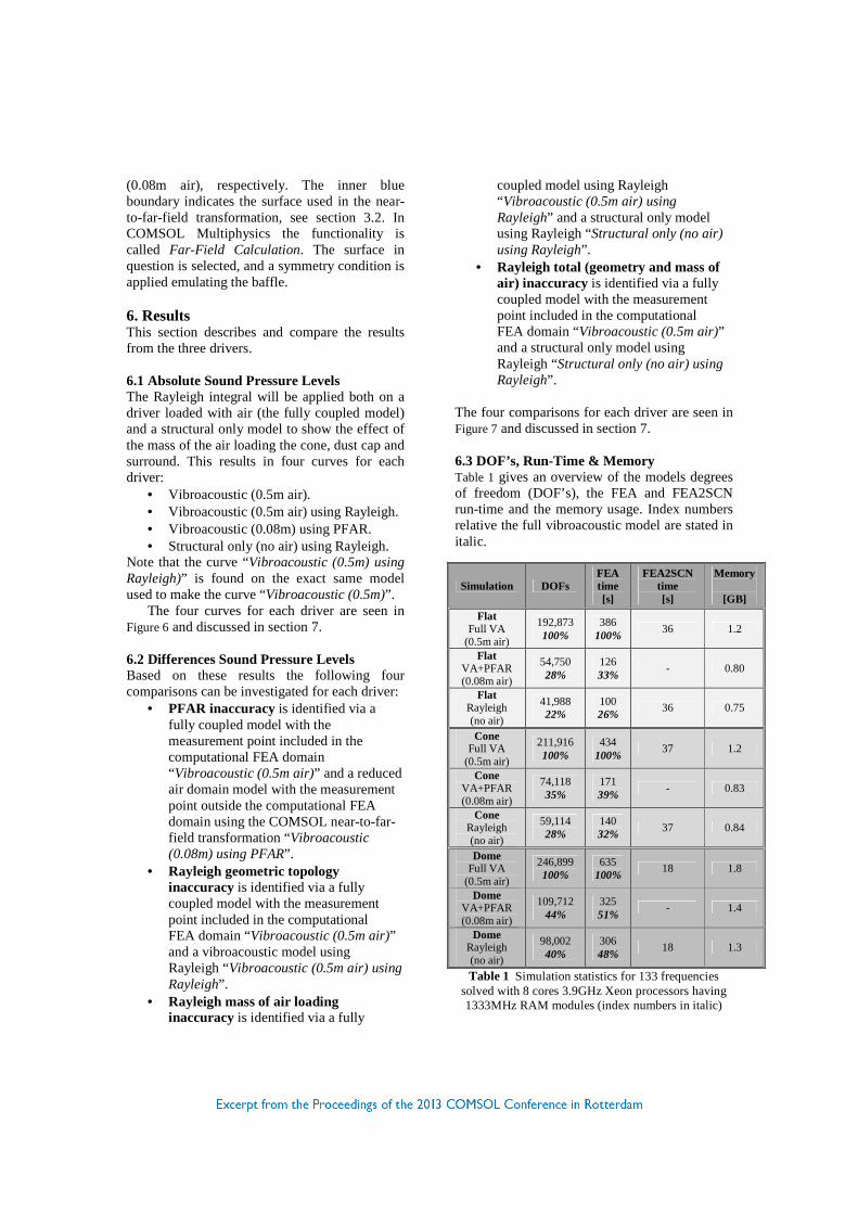
The four comparisons for each driver are seen in Figure 7 and discussed in section 7. 6.3 DOF’s, Run-Time & Memory Table 1 gives an overview of the models degrees of freedom (DOF’s), the FEA and FEA2SCN run-time and the memory usage. Index numbers relative the full vibroacoustic model are stated in italic.

Table 1 Simulation statistics for 133 frequencies solved with 8 cores 3.9GHz Xeon processors having 1333MHz RAM modules (index numbers in italic)

Simulation DOFs FEA time [s]

FEA2SCN time [s]

Memory

[GB]

Flat Full VA

(0.5m air)

192,873 100%

386 100%

36 1.2

Flat VA+PFAR (0.08m air)

54,750 28%

126 33%

- 0.80

Flat Rayleigh (no air)

41,988 22%

100 26%

36 0.75

Cone Full VA

(0.5m air)

211,916 100%

434 100%

37 1.2

Cone VA+PFAR (0.08m air)

74,118 35%

171 39%

- 0.83

Cone Rayleigh (no air)

59,114 28%

140 32%

37 0.84

Dome Full VA

(0.5m air)

246,899 100%

635 100%

18 1.8

Dome VA+PFAR (0.08m air)

109,712 44%

325 51%

- 1.4

Dome Rayleigh (no air)

98,002 40%

306 48%

18 1.3

Figure 6 Sound pressure level for all drivers

Figure 7 Differences for all drivers

7. Observations Firstly, based on the results in section 5 it is observed for all drivers, that the “PFAR inaccuracy” is negligible below ±0.5dB and it reduces the FEA run-time between 30-50%.

Secondly, it is observed on the “Rayleigh geometric topology inaccuracy” for the flat driver that the difference is practically zero. This proof correct implementations of both:

• the novel iCapture FEA2SCN program transforming the unstructured FEA-mesh to the structured scanner-grid and

• the available Klippels scanners Rayleigh calculation.

This means the used method to calculate the Rayleigh results are reliable and it is observed to reduce the FEA run-time between 26-46%.

Thirdly, it is noted if the “FEA2SCN run-time” is added to the “FEA run-time” the reduced run-time for applying the Rayleigh integral is identical with the PFAR calculations when the air domain is limited to only include the structural domain. Fourthly, it is observed for the “Rayleigh geometric topology inaccuracy” for the concave cone and convex dome drivers that the difference is frequency dependent and more than ±5.0dB for certain frequencies! Fifthly, it is observed on the “Rayleigh mass of air loading inaccuracy” that the flat driver is most sensitive with a frequency dependent variation of typically ±1.5dB between the peaks and maximum of +5dB at the peaks. The large variation at the peaks is due to the peak location is shifted upwards by the lack of moving air mass in the structural only model. For the cone and dome drivers the “Rayleigh mass of air loading inaccuracy” is observed also to be frequency dependent and typically less than ±1.0dB. Sixthly, it is observed that the “Rayleigh total inaccuracy” for all drivers shown is more than ±5dB and based on above observations it is understood that it can either be caused by the missing mass of the loading air or the geometric topology.

8. Conclusions Based on the results and observations it is concluded:

1) A reduced vibroacoustic model using PFAR excluding the measurement point in the computational FEA domain is practically identical to a full vibroacoustic model including the measurement point and it reduces the FEA run-time to 30-50%.

2) That the novel iCapture FEA2SCN program combined with the Klippel scanner software correctly calculate the Rayleigh integral and it reduces the FEA run-time 26-48%.

3) That the used Rayleigh calculation technique has identical calculation reductions of 30-50% as the COMSOL PFAR technique, when the air domain is limited to only include the structural domain.

4) A structural only model being not totally flat using Rayleigh cannot be recommended for driver design and development since frequency dependent errors of more than ±5.0dB.

So despite a tempting reduction to 30-50% run-time (i.e. an efficiency improvement of 50-70%) for 2D axisymmetric models by use of the Rayleigh integral this unfortunately leads to fundamental behaviour is not captured correctly in the vital transition band from pistonic movement to the multimode range as for example the rim resonance behaviour, which the use of FEA is intended for. The root cause is the missing air mass loading and/or the geometric non-flat topology smearing the result.

Disregarding the shifting of the peaks due to the omitted air mass on the fluid structure interface the most dominant error is caused by the geometric non-flat topology unacceptably violating the totally flat topology restriction of the Rayleigh method.

Simulation tools not able to validate this error will results in faulty and unreliable decisions-making during the design and product development, which is evident looking at the sound pressure level curves in Figure 6 of the full vibroacoustic models (the full line or the PFAR dotted gray line) and the Rayleigh based results (the dashed line).

However, when this is generally concluded it is acknowledged that for 3D models the reduction by use of the Rayleigh integral can drop down to 5-10% of the run-time of a fully coupled vibroacoustic 3D model – i.e. reduction from 25-100 days to hours.

This is in fairness a significant and ground-breaking enabler for simulation on 3D models with cyclic periodic or random geometric patterns on the cone, dust cap, surround, spider or back volume.

Having this in mind a Rayleigh approach is acceptable if the driver is almost totally flat or if – and only if – the error is identified for the specific application before the Rayleigh method is applied. 9. References 1. P. Macey, Accuracy issues in finite element simulation of loudspeakers, Audio Engineering Society Convention Paper 7600, 1-6 (2008) 2. L. E. Kinsler, A. R. Frey, A. B. Coppens, and J. V. Sanders, Fundamentals of Acoustics, 3rd Edition, Wiley, New York, (1982). 3. Klippel Scanner Software use for Rayleigh calcualations and decomposition: http://www.klippel.de/our-products/rd-system/modules/scanning-vibrometer-system.html 4. J. W. S. Rayleigh, The Theory of Sound, Vol.2, 2nd Edition, 1896. i Many designers simulate more than 1m of air to enable a standard measurement point in 1m.It is noted that the use of more than 1.0m air will decrease the run-time statistics in Table 1 by more than a factor 4 for the PFAR and Rayleigh models since the run-time of the full models will increase by the same factor or more.