
Chris Volinsky
8
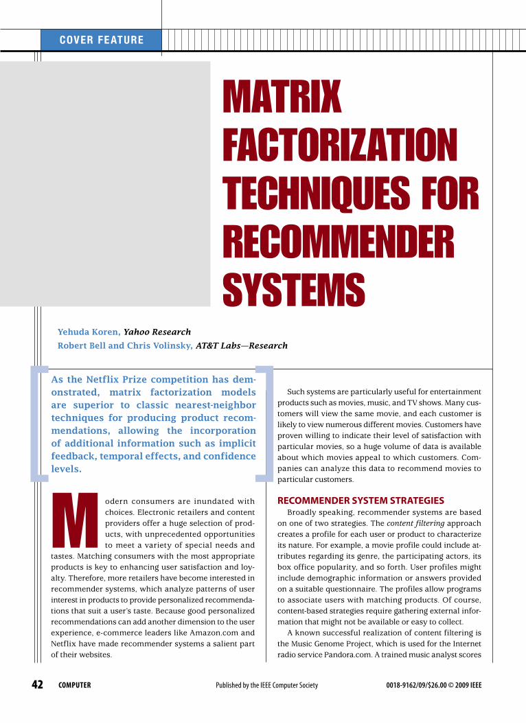
COMPUTER 42 COVER FEATURE Published by the IEEE Computer Society 0018-9162/09/$26.00 © 2009 IEEE Such systems are particularly useful for entertainment products such as movies, music, and TV shows. Many cus- tomers will view the same movie, and each customer is likely to view numerous different movies. Customers have proven willing to indicate their level of satisfaction with particular movies, so a huge volume of data is available about which movies appeal to which customers. Com- panies can analyze this data to recommend movies to particular customers. RECOMMENDER SYSTEM STRATEGIES Broadly speaking, recommender systems are based on one of two strategies. The content filtering approach creates a profile for each user or product to characterize its nature. For example, a movie profile could include at- tributes regarding its genre, the participating actors, its box office popularity, and so forth. User profiles might include demographic information or answers provided on a suitable questionnaire. The profiles allow programs to associate users with matching products. Of course, content-based strategies require gathering external infor- mation that might not be available or easy to collect. A known successful realization of content filtering is the Music Genome Project, which is used for the Internet radio service Pandora.com. A trained music analyst scores M odern consumers are inundated with choices. Electronic retailers and content providers offer a huge selection of prod- ucts, with unprecedented opportunities to meet a variety of special needs and tastes. Matching consumers with the most appropriate products is key to enhancing user satisfaction and loy- alty. Therefore, more retailers have become interested in recommender systems, which analyze patterns of user interest in products to provide personalized recommenda- tions that suit a user’s taste. Because good personalized recommendations can add another dimension to the user experience, e-commerce leaders like Amazon.com and Netflix have made recommender systems a salient part of their websites. As the Netflix Prize competition has dem- onstrated, matrix factorization models are superior to classic nearest-neighbor techniques for producing product recom- mendations, allowing the incorporation of additional information such as implicit feedback, temporal effects, and confidence levels. Yehuda Koren, Yahoo Research Robert Bell and Chris Volinsky, AT&T Labs—Research MATRIX FACTORIZATION TECHNIQUES FOR RECOMMENDER SYSTEMS
-
Upload
phungkhanh -
Category
Documents
-
view
221 -
download
1
Transcript of Chris Volinsky
computer 42
COVER FE ATURE
Published by the IEEE Computer Society 0018-9162/09/$26.00 © 2009 IEEE
Such systems are particularly useful for entertainment products such as movies, music, and TV shows. Many cus-tomers will view the same movie, and each customer is likely to view numerous different movies. Customers have proven willing to indicate their level of satisfaction with particular movies, so a huge volume of data is available about which movies appeal to which customers. Com-panies can analyze this data to recommend movies to particular customers.
RecommendeR system stRategiesBroadly speaking, recommender systems are based
on one of two strategies. The content filtering approach creates a profile for each user or product to characterize its nature. For example, a movie profile could include at-tributes regarding its genre, the participating actors, its box office popularity, and so forth. User profiles might include demographic information or answers provided on a suitable questionnaire. The profiles allow programs to associate users with matching products. Of course, content-based strategies require gathering external infor-mation that might not be available or easy to collect.
A known successful realization of content filtering is the Music Genome Project, which is used for the Internet radio service Pandora.com. A trained music analyst scores
Modern consumers are inundated with choices. Electronic retailers and content providers offer a huge selection of prod-ucts, with unprecedented opportunities to meet a variety of special needs and
tastes. Matching consumers with the most appropriate products is key to enhancing user satisfaction and loy-alty. Therefore, more retailers have become interested in recommender systems, which analyze patterns of user interest in products to provide personalized recommenda-tions that suit a user’s taste. Because good personalized recommendations can add another dimension to the user experience, e-commerce leaders like Amazon.com and Netflix have made recommender systems a salient part of their websites.
As the Netflix Prize competition has dem-onstrated, matrix factorization models are superior to classic nearest-neighbor techniques for producing product recom-mendations, allowing the incorporation of additional information such as implicit feedback, temporal effects, and confidence levels.
Yehuda Koren, Yahoo Research
Robert Bell and Chris Volinsky, AT&T Labs—Research
MATRIX FACTORIZATION TECHNIQUES FOR RECOMMENDER SYSTEMS
43AuGuSt 2009
well-defined dimensions such as depth of character de-velopment or quirkiness; or completely uninterpretable dimensions. For users, each factor measures how much the user likes movies that score high on the correspond-ing movie factor.
Figure 2 illustrates this idea for a simplified example in two dimensions. Consider two hypothetical dimen-sions characterized as female- versus male-oriented and serious versus escapist. The figure shows where several well-known movies and a few fictitious users might fall on these two dimensions. For this model, a user’s predicted rating for a movie, relative to the movie’s average rating, would equal the dot product of the movie’s and user’s lo-cations on the graph. For example, we would expect Gus to love Dumb and Dumber, to hate The Color Purple, and to rate Braveheart about average. Note that some mov-ies—for example, Ocean’s 11—and users—for example, Dave—would be characterized as fairly neutral on these two dimensions.
matRix factoRization methodsSome of the most successful realizations of latent factor
models are based on matrix factorization. In its basic form, matrix factorization characterizes both items and users by vectors of factors inferred from item rating patterns. High correspondence between item and user factors leads to a
each song in the Music Genome Project based on hundreds of distinct musical characteristics. These attributes, or genes, capture not only a song’s musical identity but also many significant qualities that are relevant to understanding listeners’ musi-cal preferences.
An alternative to content filtering relies only on past user behavior—for example, previous transactions or product ratings—without requiring the creation of explicit profiles. This approach is known as col-laborative filtering, a term coined by the developers of Tapestry, the first recom-mender system.1 Collaborative filtering analyzes relationships between users and interdependencies among products to identify new user-item associations.
A major appeal of collaborative fil-tering is that it is domain free, yet it can address data aspects that are often elusive and difficult to profile using content filter-ing. While generally more accurate than content-based techniques, collaborative filtering suffers from what is called the cold start problem, due to its inability to ad-dress the system’s new products and users. In this aspect, content filtering is superior.
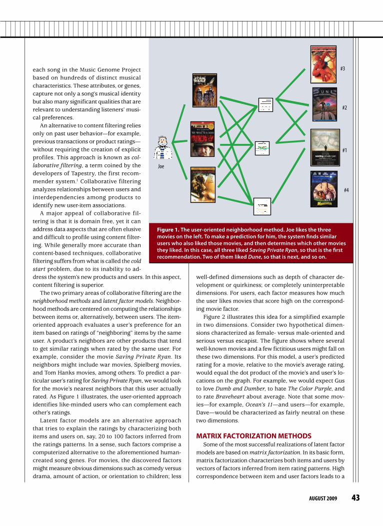
The two primary areas of collaborative filtering are the neighborhood methods and latent factor models. Neighbor-hood methods are centered on computing the relationships between items or, alternatively, between users. The item-oriented approach evaluates a user’s preference for an item based on ratings of “neighboring” items by the same user. A product’s neighbors are other products that tend to get similar ratings when rated by the same user. For example, consider the movie Saving Private Ryan. Its neighbors might include war movies, Spielberg movies, and Tom Hanks movies, among others. To predict a par-ticular user’s rating for Saving Private Ryan, we would look for the movie’s nearest neighbors that this user actually rated. As Figure 1 illustrates, the user-oriented approach identifies like-minded users who can complement each other’s ratings.
Latent factor models are an alternative approach that tries to explain the ratings by characterizing both items and users on, say, 20 to 100 factors inferred from the ratings patterns. In a sense, such factors comprise a computerized alternative to the aforementioned human-created song genes. For movies, the discovered factors might measure obvious dimensions such as comedy versus drama, amount of action, or orientation to children; less
Joe
#2
#3
#1
#4
figure 1. The user-oriented neighborhood method. Joe likes the three movies on the left. To make a prediction for him, the system finds similar users who also liked those movies, and then determines which other movies they liked. In this case, all three liked Saving Private Ryan, so that is the first recommendation. Two of them liked Dune, so that is next, and so on.

COVER FE ATURE
computer 44
vector qi ∈ f, and each user u is associ-
ated with a vector pu ∈ f. For a given item
i, the elements of qi measure the extent to
which the item possesses those factors, positive or negative. For a given user u, the elements of p
u measure the extent of
interest the user has in items that are high on the corresponding factors, again, posi-tive or negative. The resulting dot product, q
iT p
u, captures the interaction between user
u and item i—the user’s overall interest in the item’s characteristics. This approximates user u’s rating of item i, which is denoted by r
ui, leading to the estimate r̂ui
= qiT p
u. (1)
The major challenge is computing the map-ping of each item and user to factor vectors q
i, p
u ∈ f. After the recommender system
completes this mapping, it can easily esti-mate the rating a user will give to any item by using Equation 1.
Such a model is closely related to singular value decom-position (SVD), a well-established technique for identifying latent semantic factors in information retrieval. Applying SVD in the collaborative filtering domain requires factoring the user-item rating matrix. This often raises difficulties due to the high portion of missing values caused by sparse-ness in the user-item ratings matrix. Conventional SVD is undefined when knowledge about the matrix is incom-plete. Moreover, carelessly addressing only the relatively few known entries is highly prone to overfitting.
Earlier systems relied on imputation to fill in missing ratings and make the rating matrix dense.2 However, im-putation can be very expensive as it significantly increases the amount of data. In addition, inaccurate imputation might distort the data considerably. Hence, more recent works3-6 suggested modeling directly the observed rat-ings only, while avoiding overfitting through a regularized model. To learn the factor vectors (p
u and q
i), the system
minimizes the regularized squared error on the set of known ratings:
min* *,q p ( , )u i ∈
∑κ
(rui - q
iTp
u)2 + λ(|| q
i ||2 + || p
u ||2) (2)
Here, κ is the set of the (u,i) pairs for which rui is known
(the training set). The system learns the model by fitting the previously
observed ratings. However, the goal is to generalize those previous ratings in a way that predicts future, unknown ratings. Thus, the system should avoid overfitting the observed data by regularizing the learned parameters, whose magnitudes are penalized. The constant λ controls
recommendation. These methods have become popular in recent years by combining good scalability with predictive accuracy. In addition, they offer much flexibility for model-ing various real-life situations.
Recommender systems rely on different types of input data, which are often placed in a matrix with one dimension representing users and the other dimension representing items of interest. The most convenient data is high-quality explicit feedback, which includes explicit input by users regarding their interest in products. For example, Netflix collects star ratings for movies, and TiVo users indicate their preferences for TV shows by pressing thumbs-up and thumbs-down buttons. We refer to explicit user feedback as ratings. Usually, explicit feedback com-prises a sparse matrix, since any single user is likely to have rated only a small percentage of possible items.
One strength of matrix factorization is that it allows incorporation of additional information. When explicit feedback is not available, recommender systems can infer user preferences using implicit feedback, which indirectly reflects opinion by observing user behavior including pur-chase history, browsing history, search patterns, or even mouse movements. Implicit feedback usually denotes the presence or absence of an event, so it is typically repre-sented by a densely filled matrix.
a Basic matRix factoRization modeL Matrix factorization models map both users and items
to a joint latent factor space of dimensionality f, such that user-item interactions are modeled as inner products in that space. Accordingly, each item i is associated with a
Gearedtowardmales
Serious
Escapist
The PrincessDiaries
Braveheart
Lethal Weapon
IndependenceDay
Ocean’s 11Sense andSensibility
Gus
Dave
Gearedtoward
females
Amadeus
The Lion KingDumb and
Dumber
The Color Purple
figure 2. A simplified illustration of the latent factor approach, which characterizes both users and movies using two axes—male versus female and serious versus escapist.

45AuGuSt 2009
data aspects and other application-specific requirements. This requires accommodations to Equation 1 while staying within the same learning framework. Equation 1 tries to cap-ture the interactions between users and items that produce the different rating values. However, much of the observed variation in rating values is due to effects associated with either users or items, known as biases or intercepts, indepen-dent of any interactions. For example, typical collaborative filtering data exhibits large systematic tendencies for some users to give higher ratings than others, and for some items to receive higher ratings than others. After all, some products are widely perceived as better (or worse) than others.
Thus, it would be unwise to explain the full rating value by an interaction of the form q
iTp
u. Instead, the system tries
to identify the portion of these values that individual user or item biases can explain, subjecting only the true interaction portion of the data to factor modeling. A first-order approxi-mation of the bias involved in rating r
ui is as follows:
bui = µ + b
i + b
u (3)
The bias involved in rating rui is denoted by b
ui and ac-
counts for the user and item effects. The overall average rating is denoted by µ; the parameters b
u and b
i indicate
the observed deviations of user u and item i, respectively, from the average. For example, suppose that you want a first-order estimate for user Joe’s rating of the movie Titanic. Now, say that the average rating over all movies, µ, is 3.7 stars. Furthermore, Titanic is better than an average movie, so it tends to be rated 0.5 stars above the average. On the other hand, Joe is a critical user, who tends to rate 0.3 stars lower than the average. Thus, the estimate for Titanic’s rating by Joe would be 3.9 stars (3.7 + 0.5 - 0.3). Biases extend Equation 1 as follows:
r̂ui = µ+ b
i + b
u + q
iTp
u (4)
Here, the observed rating is broken down into its four components: global average, item bias, user bias, and user-item interaction. This allows each component to explain only the part of a signal relevant to it. The system learns by minimizing the squared error function:4,5
min* * *, ,p q b
( , )u i ∈∑
κ
(rui - µ - b
u - b
i - p
uTq
i)2 + λ
(|| p
u ||2 + || q
i ||2 + b
u2 + b
i2) (5)
Since biases tend to capture much of the observed signal, their accurate modeling is vital. Hence, other works offer more elaborate bias models.11
additionaL inPUt soURces Often a system must deal with the cold start problem,
wherein many users supply very few ratings, making it
the extent of regularization and is usually determined by cross-validation. Ruslan Salakhutdinov and Andriy Mnih’s “Probabilistic Matrix Factorization”7 offers a probabilistic foundation for regularization.
LeaRning aLgoRithms Two approaches to minimizing Equation 2 are stochastic
gradient descent and alternating least squares (ALS).
stochastic gradient descent Simon Funk popularized a stochastic gradient descent
optimization of Equation 2 (http://sifter.org/~simon/journal/20061211.html) wherein the algorithm loops through all ratings in the training set. For each given training case, the system predicts r
ui and computes the
associated prediction error
eui =
def
rui - q
iT p
u.
Then it modifies the parameters by a magnitude pro-portional to g in the opposite direction of the gradient, yielding:
• q q e p qi i ui u i← + ⋅ ⋅ - ⋅g λ( ) • p p e q pu u ui i u← + ⋅ ⋅ - ⋅g λ( )
This popular approach4-6 combines implementation ease with a relatively fast running time. Yet, in some cases, it is beneficial to use ALS optimization.
alternating least squares Because both q
i and p
u are unknowns, Equation 2 is not
convex. However, if we fix one of the unknowns, the op-timization problem becomes quadratic and can be solved optimally. Thus, ALS techniques rotate between fixing the q
i’s and fixing the p
u’s. When all p
u’s are fixed, the system
recomputes the qi’s by solving a least-squares problem, and
vice versa. This ensures that each step decreases Equation 2 until convergence.8
While in general stochastic gradient descent is easier and faster than ALS, ALS is favorable in at least two cases. The first is when the system can use parallelization. In ALS, the system computes each q
i independently of the other
item factors and computes each pu independently of the
other user factors. This gives rise to potentially massive parallelization of the algorithm.9 The second case is for systems centered on implicit data. Because the training set cannot be considered sparse, looping over each single training case—as gradient descent does—would not be practical. ALS can efficiently handle such cases.10
adding Biases One benefit of the matrix factorization approach to col-
laborative filtering is its flexibility in dealing with various

COVER FE ATURE
computer 46
prove accuracy. Decomposing ratings into distinct terms allows the system to treat different temporal aspects sepa-rately. Specifically, the following terms vary over time: item biases, b
i(t); user biases, b
u(t); and user preferences, p
u(t).
The first temporal effect addresses the fact that an item’s popularity might change over time. For example, movies can go in and out of popularity as triggered by external events such as an actor’s appearance in a new movie. Therefore, these models treat the item bias b
i as a
function of time. The second temporal effect allows users to change their baseline ratings over time. For example, a user who tended to rate an average movie “4 stars” might now rate such a movie “3 stars.” This might reflect several factors including a natural drift in a user’s rating scale, the fact that users assign ratings relative to other recent ratings, and the fact that the rater’s identity within a house-hold can change over time. Hence, in these models, the parameter b
u is a function of time.
Temporal dynamics go beyond this; they also affect user preferences and therefore the interaction between users and items. Users change their preferences over time. For example, a fan of the psychological thrillers genre might become a fan of crime dramas a year later. Simi-larly, humans change their perception of certain actors and directors. The model accounts for this effect by taking the user factors (the vector p
u) as a function of time. On
the other hand, it specifies static item characteristics, qi,
because, unlike humans, items are static in nature. Exact parameterizations of time-varying parameters11
lead to replacing Equation 4 with the dynamic prediction rule for a rating at time t:
r̂ui (t) = µ + b
i(t) + b
u(t) + q
iT p
u(t) (7)
inPUts With VaRying confidence LeVeLs In several setups, not all observed ratings deserve the
same weight or confidence. For example, massive adver-tising might influence votes for certain items, which do not aptly reflect longer-term characteristics. Similarly, a system might face adversarial users that try to tilt the rat-ings of certain items.
Another example is systems built around implicit feedback. In such systems, which interpret ongoing user behavior, a user’s exact preference level is hard to quantify. Thus, the system works with a cruder binary representation, stating either “probably likes the product” or “probably not interested in the product.” In such cases, it is valuable to attach confidence scores with the esti-mated preferences. Confidence can stem from available numerical values that describe the frequency of actions, for example, how much time the user watched a certain show or how frequently a user bought a certain item. These numerical values indicate the confidence in each obser-vation. Various factors that have nothing to do with user
difficult to reach general conclusions on their taste. A way to relieve this problem is to incorporate additional sources of information about the users. Recommender systems can use implicit feedback to gain insight into user preferences. Indeed, they can gather behavioral information regardless of the user’s willingness to provide explicit ratings. A re-tailer can use its customers’ purchases or browsing history to learn their tendencies, in addition to the ratings those customers might supply.
For simplicity, consider a case with a Boolean implicit feedback. N(u) denotes the set of items for which user u expressed an implicit preference. This way, the system profiles users through the items they implicitly preferred. Here, a new set of item factors are necessary, where item i is associated with x
i ∈ f. Accordingly, a user who
showed a preference for items in N(u) is characterized by the vector
xi
i N u∈∑
( )
.
Normalizing the sum is often beneficial, for example, working with
|N(u)|–0.5 xi
i N u∈∑
( )
.4,5
Another information source is known user attributes, for example, demographics. Again, for simplicity consider Boolean attributes where user u corresponds to the set of attributes A(u), which can describe gender, age group, Zip code, income level, and so on. A distinct factor vector y
a ∈ f corresponds to each attribute to describe a user
through the set of user-associated attributes:
ya
a A u∈∑
( )
The matrix factorization model should integrate all signal sources, with enhanced user representation:
r̂ui = µ + b
i + b
u + q
iT [p
u + |N(u)|–0.5 x yi a
i N u a A u∈ ∈∑ ∑+
( ) ( )
] (6) While the previous examples deal with enhancing user
representation—where lack of data is more common—items can get a similar treatment when necessary.
temPoRaL dynamics So far, the presented models have been static. In real-
ity, product perception and popularity constantly change as new selections emerge. Similarly, customers’ inclina-tions evolve, leading them to redefine their taste. Thus, the system should account for the temporal effects re-flecting the dynamic, time-drifting nature of user-item interactions.
The matrix factorization approach lends itself well to modeling temporal effects, which can significantly im-

47AuGuSt 2009
Our winning entries consist of more than 100 differ-ent predictor sets, the majority of which are factorization models using some variants of the methods described here. Our discussions with other top teams and postings on the public contest forum indicate that these are the most popu-lar and successful methods for predicting ratings.
Factorizing the Netflix user-movie matrix allows us to discover the most descriptive dimensions for predict-ing movie preferences. We can identify the first few most important dimensions from a matrix decomposition and explore the movies’ location in this new space. Figure 3 shows the first two factors from the Netflix data matrix factorization. Movies are placed according to their factor vectors. Someone familiar with the movies shown can see clear meaning in the latent factors. The first factor vector (x-axis) has on one side lowbrow comedies and horror movies, aimed at a male or adolescent audience (Half Baked, Freddy vs. Jason), while the other side contains drama or comedy with serious undertones and strong female leads (Sophie’s Choice, Moonstruck). The second factorization axis (y-axis) has independent, critically acclaimed, quirky films (Punch-Drunk Love, I Heart Huckabees) on the top, and on the bottom, mainstream formulaic films (Armaged-don, Runaway Bride). There are interesting intersections between these boundaries: On the top left corner, where indie meets lowbrow, are Kill Bill and Natural Born Kill-ers, both arty movies that play off violent themes. On the bottom right, where the serious female-driven movies meet
preferences might cause a one-time event; however, a recurring event is more likely to reflect user opinion.
The matrix factorization model can readily accept varying confidence levels, which let it give less weight to less meaningful observations. If con-fidence in observing r
ui is denoted as
cui, then the model enhances the cost
function (Equation 5) to account for confidence as follows:
min* * *, ,p q b
( , )u i ∈∑
κ
cui(r
ui - µ - b
u - b
i
- pu
Tqi)2 + λ (|| p
u ||2 + || q
i ||2
+ bu
2 + bi2) (8)
For information on a real-life ap-plication involving such schemes, refer to “Collaborative Filtering for Implicit Feedback Datasets.”10
netfLix PRize comPetition
In 2006, the online DVD rental company Netflix announced a con-test to improve the state of its recommender system.12 To enable this, the company released a training set of more than 100 million ratings spanning about 500,000 anony-mous customers and their ratings on more than 17,000 movies, each movie being rated on a scale of 1 to 5 stars. Participating teams submit predicted ratings for a test set of approximately 3 million ratings, and Netflix calculates a root-mean -square error (RMSE) based on the held-out truth. The first team that can improve on the Netflix algo-rithm’s RMSE performance by 10 percent or more wins a $1 million prize. If no team reaches the 10 percent goal, Netflix gives a $50,000 Progress Prize to the team in first place after each year of the competition.
The contest created a buzz within the collaborative fil-tering field. Until this point, the only publicly available data for collaborative filtering research was orders of magni-tude smaller. The release of this data and the competition’s allure spurred a burst of energy and activity. According to the contest website (www.netflixprize.com), more than 48,000 teams from 182 different countries have down-loaded the data.
Our team’s entry, originally called BellKor, took over the top spot in the competition in the summer of 2007, and won the 2007 Progress Prize with the best score at the time: 8.43 percent better than Netflix. Later, we aligned with team Big Chaos to win the 2008 Progress Prize with a score of 9.46 percent. At the time of this writing, we are still in first place, inching toward the 10 percent landmark.
–1.5 –1.0 –0.5 0.0 0.5 1.0
–1.5
–1.0
–0.5
0.0
0.5
1.0
1.5
Factor vector 1
Facto
r vec
tor 2
Freddy Got Fingered
Freddy vs. Jason
Half Baked
Road Trip
The Sound of Music
Sophie’s Choice
Moonstruck
Maid in Manhattan
The Way We Were
Runaway Bride
Coyote Ugly
The Royal Tenenbaums
Punch-Drunk Love
I Heart Huckabees
Armageddon
Citizen Kane
The Waltons: Season 1
Stepmom
Julien Donkey-Boy
Sister A
ct
The Fast and the Furious
The Wizard of Oz
Kill Bill:
Vol. 1
ScarfaceNatural Born Kille
rs
Annie Hall
Belle de JourLost i
n Translation
The Longest Yard
Being John Malkovich
Catwoman
figure 3. The first two vectors from a matrix decomposition of the Netflix Prize data. Selected movies are placed at the appropriate spot based on their factor vectors in two dimensions. The plot reveals distinct genres, including clusters of movies with strong female leads, fraternity humor, and quirky independent films.
COVER FE ATURE
computer 48
Matrix factoriza-tion techniques have become a dominant meth-odology within
collaborative filtering recom-menders. Experience with datasets such as the Netflix Prize data has shown that they deliver accuracy superior to classical nearest-neighbor techniques. At the same time, they offer a com-pact memory-efficient model that systems can learn relatively easily. What makes these tech-niques even more convenient is that models can integrate natu-rally many crucial aspects of the data, such as multiple forms of feedback, temporal dynamics, and confidence levels.
References 1. D. Goldberg et al., “Using Col- laborative Filtering to Weave an Information Tapestry,” Comm. ACM, vol. 35, 1992, pp. 61-70.
2. B.M. Sarwar et al., “Application of Dimensionality Reduc-tion in Recommender System—A Case Study,” Proc. KDD Workshop on Web Mining for e-Commerce: Challenges and Opportunities (WebKDD), ACM Press, 2000.
3. S. Funk, “Netflix Update: Try This at Home,” Dec. 2006; http://sifter.org/~simon/journal/20061211.html.
4. Y. Koren, “Factorization Meets the Neighborhood: A Mul-tifaceted Collaborative Filtering Model,” Proc. 14th ACM SIGKDD Int’l Conf. Knowledge Discovery and Data Mining, ACM Press, 2008, pp. 426-434.
5. A. Paterek, “Improving Regularized Singular Value De-composition for Collaborative Filtering,” Proc. KDD Cup and Workshop, ACM Press, 2007, pp. 39-42.
6. G. Takács et al., “Major Components of the Gravity Recom-mendation System,” SIGKDD Explorations, vol. 9, 2007, pp. 80-84.
7. R. Salakhutdinov and A. Mnih, “Probabilistic Matrix Fac-torization,” Proc. Advances in Neural Information Processing Systems 20 (NIPS 07), ACM Press, 2008, pp. 1257-1264.
8. R. Bell and Y. Koren, “Scalable Collaborative Filtering with Jointly Derived Neighborhood Interpolation Weights,” Proc. IEEE Int’l Conf. Data Mining (ICDM 07), IEEE CS Press, 2007, pp. 43-52.
9. Y. Zhou et al., “Large-Scale Parallel Collaborative Filter-ing for the Netflix Prize,” Proc. 4th Int’l Conf. Algorithmic Aspects in Information and Management, LNCS 5034, Springer, 2008, pp. 337-348.
10. Y.F. Hu, Y. Koren, and C. Volinsky, “Collaborative Filtering for Implicit Feedback Datasets,” Proc. IEEE Int’l Conf. Data Mining (ICDM 08), IEEE CS Press, 2008, pp. 263-272.
the mainstream crowd-pleasers, is The Sound of Music. And smack in the middle, appealing to all types, is The Wizard of Oz.
In this plot, some movies neighboring one another typi-cally would not be put together. For example, Annie Hall and Citizen Kane are next to each other. Although they are stylistically very different, they have a lot in common as highly regarded classic movies by famous directors. Indeed, the third dimension in the factorization does end up separating these two.
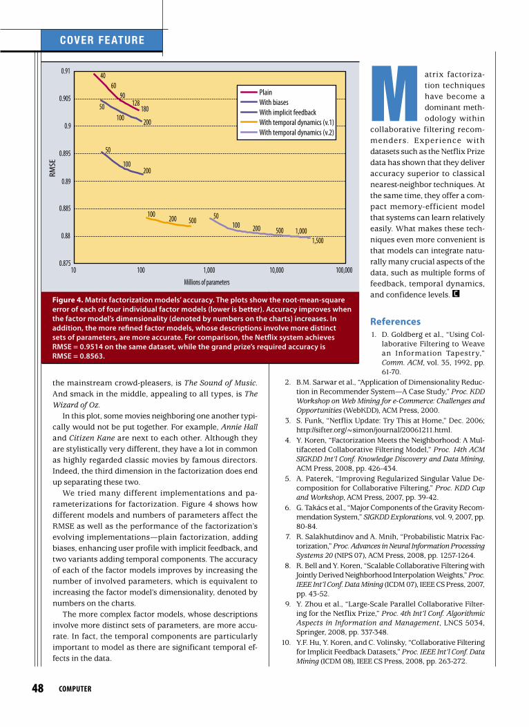
We tried many different implementations and pa-rameterizations for factorization. Figure 4 shows how different models and numbers of parameters affect the RMSE as well as the performance of the factorization’s evolving implementations—plain factorization, adding biases, enhancing user profile with implicit feedback, and two variants adding temporal components. The accuracy of each of the factor models improves by increasing the number of involved parameters, which is equivalent to increasing the factor model’s dimensionality, denoted by numbers on the charts.
The more complex factor models, whose descriptions involve more distinct sets of parameters, are more accu-rate. In fact, the temporal components are particularly important to model as there are significant temporal ef-fects in the data.
4060
90128
18050100 200
50
100200
100 200 500 50100 200 500 1,000
1,500
0.875
0.88
0.885
0.89
0.895
0.9
0.905
0.91
10 100 1,000 10,000 100,000Millions of parameters
RMSE
PlainWith biasesWith implicit feedbackWith temporal dynamics (v.1)With temporal dynamics (v.2)
figure 4. Matrix factorization models’ accuracy. The plots show the root-mean-square error of each of four individual factor models (lower is better). Accuracy improves when the factor model’s dimensionality (denoted by numbers on the charts) increases. In addition, the more refined factor models, whose descriptions involve more distinct sets of parameters, are more accurate. For comparison, the Netflix system achieves RMSE = 0.9514 on the same dataset, while the grand prize’s required accuracy is RMSE = 0.8563.

49AuGuSt 2009
Robert Bell is a principal member of the technical staff at AT&T Labs—Research. His research interests are survey research methods and statistical learning methods. He re-ceived a PhD in statistics from Stanford University. Bell is a member of the American Statistical Association and the Institute of Mathematical Statistics. Contact him at [email protected].
Chris Volinsky is director of statistics research at AT&T Labs—Research. His research interests are large-scale data mining, social networks, and models for fraud detection. He received a PhD in statistics from the University of Wash-ington. Volinsky is a member of the American Statistical Association. Contact him at [email protected].
11. Y. Koren, “Collaborative Filtering with Temporal Dynam-ics,” Proc. 15th ACM SIGKDD Int’l Conf. Knowledge Discovery and Data Mining (KDD 09), ACM Press, 2009, pp. 447-455.
12. J. Bennet and S. Lanning, “The Netflix Prize,” KDD Cup and Workshop, 2007; www.netflixprize.com.
Yehuda Koren is a senior research scientist at Yahoo Re-search, Haifa. His research interests are recommender systems and information visualization. He received a PhD in computer science from the Weizmann Institute of Science. Koren is a member of the ACM. Contact him at [email protected].