Choosing and Architecting Storage for Your...
37
Choosing and Architecting Storage for Your Environment Lucas Nguyen Technical Alliance Manager Mike DiPetrillo Specialist Systems Engineer
Transcript of Choosing and Architecting Storage for Your...

Choosing and Architecting Storage for Your Environment
Lucas Nguyen
Technical Alliance Manager
Mike DiPetrillo
Specialist Systems Engineer

Agenda
VMware Storage OptionsFibre ChannelNASiSCSIDAS
Architecture Best PracticesSizingCase Study: Impact of Architecture on Performance
Storage Mechanisms
Technology Market Transfers Interface Performance
FibreChannel
DataCenter
Block access of data/LUN FC HBA
High (due to dedicated network)
NAS SMBFile(no direct LUN access)
NICMedium (depends on integrity of LAN)
iSCSI SMB Block access of data/LUN
iSCSIHBA
Medium (depends on integrity of LAN)
DAS BranchOffice Block access SCSI HBA High (due to
dedicated bus)

Storage Mechanisms (Topology Comparison)
Branch Office SMB Market Data Center
DASDirect Attached Storage
NASNetwork Attached Storage
SANStorage Area Network
DAS vs NAS vs SAN

Storage Disaster Recovery OptionsNAS SANDAS
Tape / RAIDS/W Cluster
Tape / RAIDNIC failoverS/W Cluster Filer ClusterLAN backupData Replication
Tape / RAIDHBA / SP failoverFabric / ISL redundancyData Replication technologiesS/W Cluster within Virtual MachineLAN backup within Virtual MachineVMware HAVMware Consolidated Backup

Choosing Disks
Traditional performance factorsCapacity / Price Disk types (SCSI, ATA, FC, SATA)Access Time; IOPS; Sustained Transfer RateReliability (MTBF)
VM performance gated ultimately by IOPS density and storage spaceIOPS Density -> Number of read IOPS/GB
Higher = better
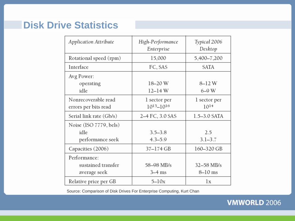
Disk Drive Statistics
Source: Comparison of Disk Drives For Enterprise Computing, Kurt Chan

Typical IOPS Density
Tier1 -> 144 GB, 15k RPM->180 IOPS/144GB = 1.25 IOPS/GBTier2 -> 300 GB, 10k RPM-> 150 IOPS/300GB = 0.5 IOPS/GBTier3 -> 500 GB, 7k RPM -> 90 IOPS/500 GB = 0.18 IOPS/GBRelative Performance
Tier1 -> 1.0Tier2 -> 0.4 (40%)Tier3 -> 0.14 (14%)
Potential choices -> FC, LC-FC, SATAII

Volume Aggregation
Stripe virtual LUN across volumes from multiple RAID 5 groups. Some storage platforms only concat, but striping is preferred.Aggregate across volumes in the same ZBR zone. Do not mix volumes from different disk sizes, rotational velocity, or volume sizes.It is OK and preferred to stripe within the same volume groups.End result is one LUNpresented to VMware spanning many physical disks.
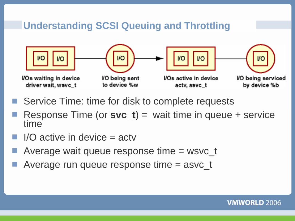
Understanding SCSI Queuing and Throttling
Service Time: time for disk to complete requestsResponse Time (or svc_t) = wait time in queue + service timeI/O active in device = actvAverage wait queue response time = wsvc_tAverage run queue response time = asvc_t

Understanding the Network Storage StackSCSI Queuing and Throttling
SCSI is a connect/disconnect protocol so the array can make certain optimizationsWait queue - I/O’s buffering in the HBA/sd queue - badActive queue – I/O’s buffered in the storage arrayService queue – I/O’s being serviced on the disk (read miss) or cache (read hit, or fast write)

SCSI and Storage Optimizations – Keep that disk busy
Array writes – written to hardware cache, destaged to disk with SCSI write buffering disabledArray reads – Array can reorder reads to minimize storage contention
SCSI tag queuing can optimize reads on active disks
Why is this important?A moderately busy disk services requests faster on whole than an inactive disk

Busy, but not backed into the HBA wait queue
Average I/O 80-100 ms which is very slow (>50 ms)
R/s w/s Kr/s kw/s wait actv wsvc_t asvc_t %w %b device Utilization Throughput
(IOPS)Av Read
Sz (K)ServTime
215.6 2.0 5799.1 29.5 0.0 20.0 0.0 91.8 0 88 c7t1d0 0.88 217.60 26.90 4.04
215.8 2.4 5814.6 38.5 0.0 15.3 0.0 69.9 0 84 c7t2d0 0.84 218.20 26.94 3.85
216.0 1.9 5814.9 30.1 0.0 15.4 0.0 70.6 0 84 c7t3d0 0.84 217.90 26.92 3.85
217.6 2.1 5820.9 32.0 0.0 25.0 0.0 113.9 0 92 c8t9d0 0.92 219.70 26.75 4.19
216.3 2.0 5803.8 31.0 0.0 18.6 0.0 85.1 0 89 c8t10d0 0.89 218.30 26.83 4.08
216.4 2.0 5801.3 29.8 0.0 18.1 0.0 83.1 0 88 c8t11d0 0.88 218.40 26.81 4.03

Flooded, I/O serialized in wait queueAverage I/O 200+ ms
r/s w/s kr/s kw/s wait actv wsvc_t asvc_t %w %b device Utilization ThroughputAv Read
SzSvcTime
Dua411
Dua461
121.3 0.7 5677.3 10.9 41.3 13.4 338.0 109.7 79 98 c6t0d0 0.98 122.00 46.80 8.03
121.2 0.6 5648.6 9.1 43 13.2 353.5 108.6 79 97 c6t1d0 0.97 121.80 46.61 7.96
120.6 0.4 5654.6 5.7 34.6 12.9 285.9 106.9 75 96 c6t2d0 0.96 121.00 46.89 7.93
121.8 0.0 5781.2 0.1 29 11.9 238.4 97.3 67 92 c6t3d0 0.92 121.80 47.46 7.55
123.0 0.0 5796.8 0.3 23.3 11.2 189.0 91.2 62 90 c6t4d0 0.90 123.00 47.13 7.32
123.8 0.0 5834.6 0.1 25.1 11.4 202.8 92.0 64 90 c6t9d0 0.90 123.80 47.13 7.27
94.9 1.1 2915.4 17.2 15.3 7.9 159.0 82.6 41 67c6t16d
0 0.67 96.00 30.72 6.98
94.6 0.8 2905.1 12.1 14 7.8 146.5 82.1 41 67c6t17d
0 0.67 95.40 30.71 7.02
95.4 0.9 2937.1 13.6 14.6 8 151.2 82.9 42 67c6t18d
0 0.67 96.30 30.79 6.96

LUN Queuing for VMware
Queuing techniques differentIn symmetric storage, path software can spread I/O’s to different adapter ports (LUN queues in adapter ports)Typical open system can have several LUNs
VMwareLUN/VMFS active on one path (active/passive arrays) onlyVMFS volume much larger than typical OS LUN
Why is this important?Default HBA queue depth usually too small

Controlling VM’s from flooding your storage
Easiest method is setting the maximum outstanding disk requests
This setting can slow a read I/O intensive VM, but will protect the farm. Problems usually surface during backup/restore
• Advanced Settings Disk.SchedNumReqOutstanding (Number of outstanding commands to a target with competing worlds) [1-256: default = 16]: 16
Do not set this to the queue depth as this is intended to throttle multiple VM’s
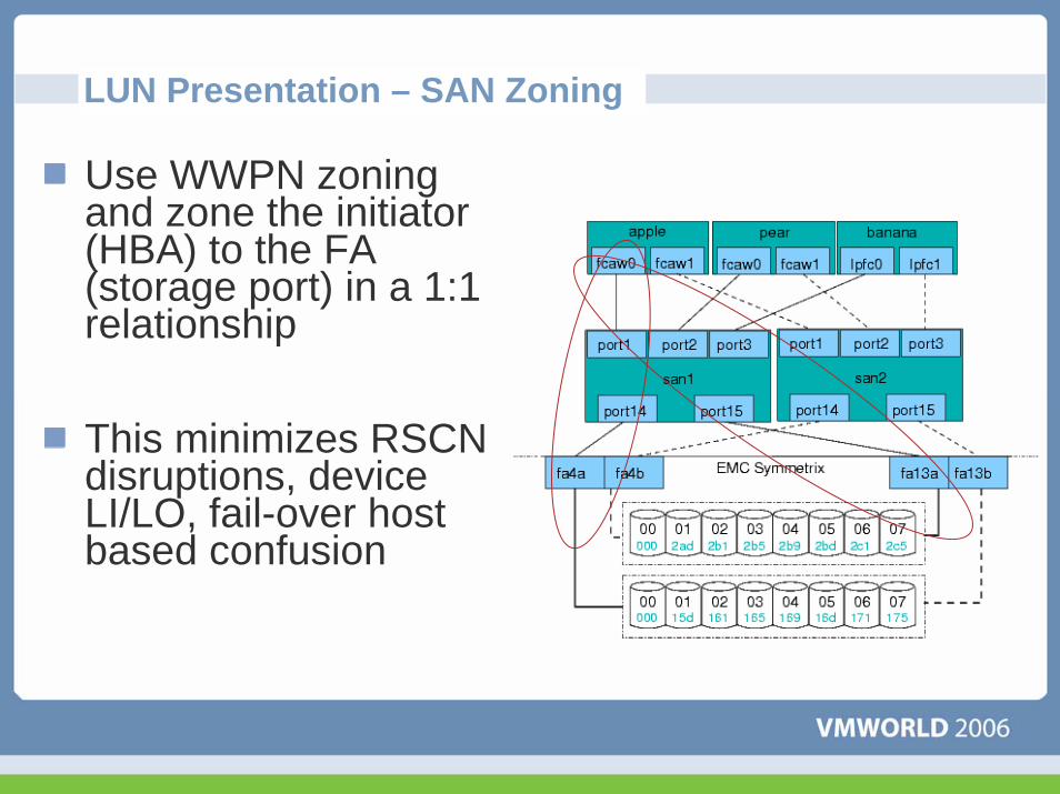
LUN Presentation – SAN Zoning
Use WWPN zoning and zone the initiator (HBA) to the FA (storage port) in a 1:1 relationship
This minimizes RSCN disruptions, device LI/LO, fail-over host based confusion

CASE STUDY
Impact of Architecture on Performance

Background
Architecture can have huge performance implicationsEvery environment will be differentUse tests in your environment to find bottlenecks

Our Current Architecture

Tests RunIOMeter
70% Random, 70% Read, 64k Block5 Minute run10 GB disk
Fibre ChannelStudent Results
Fibre ChannelPre-Run
iSCSIPre-Run
NASPre-Run
VMFS RDM VMFS RDM VMFS RDM VMDK
Total I/Os per Second(IOPS)
3294 3353 1813 1865 1691
Total MBs per Second(Throughput)
206 209 113 116 105
Average I/O Response Time (ms)
1.21 1.19 2.20 2.14 2.36
% CPU Utilization (total)
33.87% 27.26% 24.00% 19.40% 23.00%
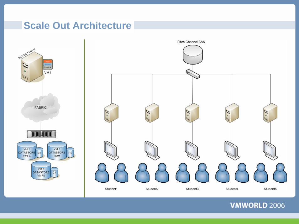
Scale Out Architecture

Results
Students got worse performanceWhere’s the bottleneck?
Fibre ChannelStudent Results
Fibre ChannelPre-Run
iSCSIPre-Run
NASPre-Run
VMFS RDM VMFS RDM VMFS RDM VMDK
Total I/Os per Second(IOPS)
1894 1868 3294 3353 1813 1865 1691
Total MBs per Second(Throughput)
110 113 206 209 113 116 105
Average I/O Response Time (ms)
1.19 1.24 1.21 1.19 2.20 2.14 2.36
% CPU Utilization (total)
22.73% 21.72% 33.87% 27.26% 24.00% 19.40% 23.00%

AnalysisiSCSI and NAS give good performanceTier your storageRDMs do not always give better performance than VMFS
(1894, 3294) for VMFS (1868, 3353) for RDM
Fibre ChannelStudent Results
Fibre ChannelPre-Run
iSCSIPre-Run
NASPre-Run
VMFS RDM VMFS RDM VMFS RDM VMDK
Total I/Os per Second(IOPS)
1894 1868 3294 3353 1813 1865 1691
Total MBs per Second(Throughput)
110 113 206 209 113 116 105
Average I/O Response Time (ms)
1.19 1.24 1.21 1.19 2.20 2.14 2.36
% CPU Utilization (total)
22.73% 21.72% 33.87% 27.26% 24.00% 19.40% 23.00%

AnalysisLocated a potential bottleneck – SP path
How could you improve performance?

Discover a Down Stream BottleneckTest to see if our path is the bottleneck
Use more downstream destinations
1 ESX Server – 1 Array – 2 Datastores

Discover a Down Stream BottleneckSplit datastores give better performance because of more work queues
Path was not our bottleneck
IOPS MB/s Latency %CPU
VM1 1961 123 2.04 22.27%
VM2 1983 123 2.01 22.37%
Total 3944 246
Previous 3294 206
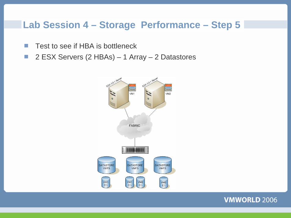
Lab Session 4 – Storage Performance – Step 5
Test to see if HBA is bottleneck2 ESX Servers (2 HBAs) – 1 Array – 2 Datastores

Lab Session 4 – Storage Performance – Step 5Still bound at path to SP
IOPS MB/s Latency %CPU
VM-Host1 1980 124 2.02 20.30%
VM-Host2 1989 124 2.01 20.70%
Total 3969 248
Previous 3944 246
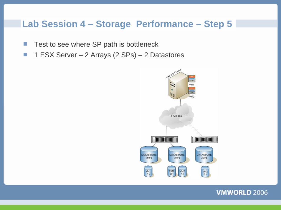
Lab Session 4 – Storage Performance – Step 5
Test to see where SP path is bottleneck1 ESX Server – 2 Arrays (2 SPs) – 2 Datastores
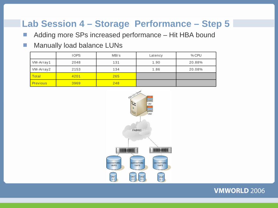
Lab Session 4 – Storage Performance – Step 5Adding more SPs increased performance – Hit HBA boundManually load balance LUNs
IOPS MB/s Latency %CPU
VM-Array1 2048 131 1.90 20.88%
VM-Array2 2153 134 1.86 20.08%
Total 4201 265
Previous 3969 248

Lab Session 4 – Storage Performance – Step 5
Test spans across volumes1 ESX Server – 1 Array – Spanned Volume

Lab Session 4 – Storage Performance – Step 5Spanned Volumes DO NOT increase performance
IOPS MB/s Latency %CPU
Student#-Storage 3328 208 1.20 32.74%
Original 3294 206

Lab Session 4 – Storage Performance – Step 5
NOTE: Every environment is different. If you decide to run this test in your environment your numbers may be different for a variety of reasons. Many things will change the results of your tests such as SAN fabric architecture, speed of disks, speed of HBAs, number of HBAs, etc. The numbers introduced in this lab are by no means meant to be an official benchmark of the lab equipment. The tests run were simply used to create a desired performance issue so that a point could be made. Please consult your storage vendor contacts for official benchmarking numbers on their arrays in a number of environments

Questions?

Presentation Download
Please remember to complete yoursession evaluation form
and return it to the room monitorsas you exit the session
The presentation for this session can be downloaded at http://www.vmware.com/vmtn/vmworld/sessions/
Enter the following to download (case-sensitive):
Username: cbv_repPassword: cbvfor9v9r

Some or all of the features in this document may be representative of feature areas under development. Feature commitments must not be included in contracts, purchase orders, or sales agreements of any kind. Technical feasibility and market demand will affect final delivery.