Choice of Criteria, plus

Blending Models in Fuel, Food, Feed, and Ferrous

University of ChicagoGraduate School of Business

Introduction to Computer Based Models Bus-36102-81Mr. Schrage Spring 2003

Deriving Proper Objective Function Coefficients:

Variable costs: This is what LP assumes.

Sunk costs: To be disregarded. What’s sunk depends upon

planning horizon.

Fixed costs: An entry fee for using an activity, regardless

of volume. Need IP to represent.

Allocated costs: To be avoided at all costs.

Joint costs: Accurately represented by LP + constraints.

Quality/Blending Constraints,

Representing and Measuring

Frequently are of form:

Ratio target,

e.g., the octane requirement for a fuel composed of three ingredients, or a constraint on the “duration” of a portfolio might be stated as:

85 86 9087

X Y Z

X Y Z

This is nonlinear. Nonlinear is bad. What to do?

Ans. 85 X + 86 Y + 90 Z 87( X + Y + Z)

What kind of vehicle is this?

A.: A truck.

Is this a ’98 or a ’99 Suburban?

A.: Yes.

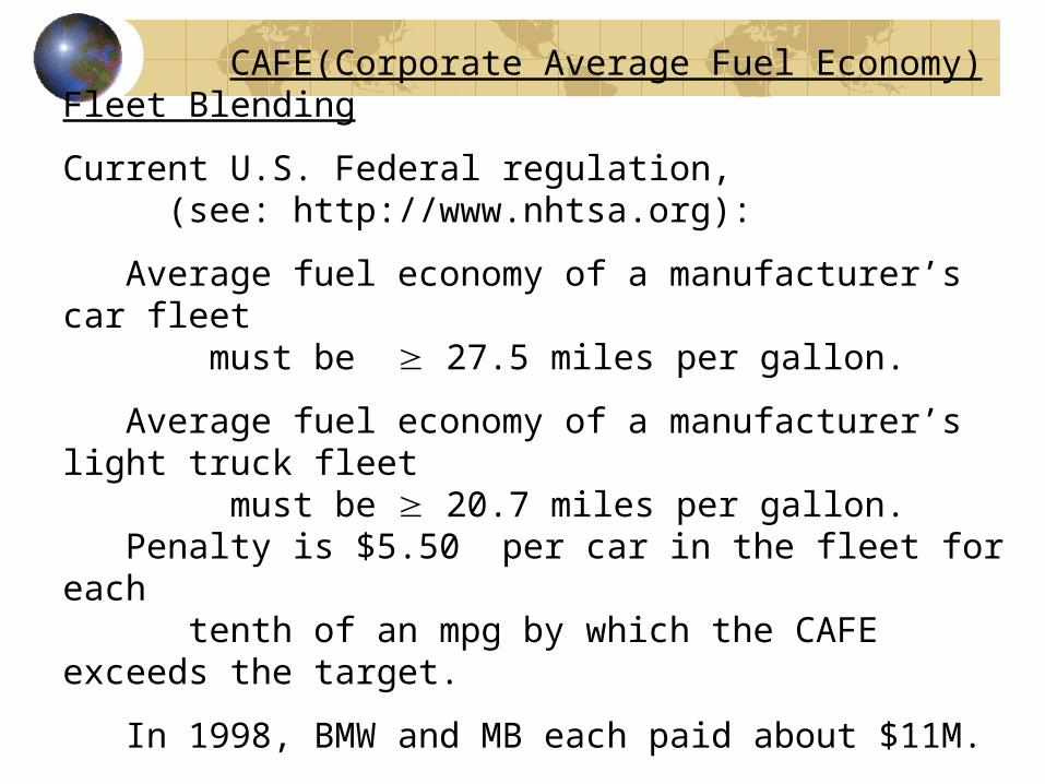
CAFE(Corporate Average Fuel Economy) Fleet Blending

Current U.S. Federal regulation, (see: http://www.nhtsa.org):

Average fuel economy of a manufacturer’s car fleet must be 27.5 miles per gallon.

Average fuel economy of a manufacturer’s light truck fleet must be 20.7 miles per gallon. Penalty is $5.50 per car in the fleet for each tenth of an mpg by which the CAFE exceeds the target.

In 1998, BMW and MB each paid about $11M.

 

Example:

Ford has four cars with the following highway mpg ratings:

Escort 33 mpg

Contour 32 mpg

Taurus 27 mpg

Lincoln Continental 24 mpg

How should one decide how many to produce and sell of each?

Making plausible assumptions about profit contributions, manufacturing capacities, and demands……

Corporate Average Fuel Efficiency model, MPG case;MAX = 1800 * ESCORTA + 2100*CONTOURA + 2000 * CONTOURB + 4100 * TAURUSB + 4000 * TAURUSC + 16000 * LINCOLNC;! Capacity constraints; [PlantA] ESCORTA + 1.1 * CONTOURA <= 100000; [PlantB] CONTOURB + 1.2 * TAURUSB <= 200000; [PlantC] TAURUSC + 1.4 * LINCOLNC <= 300000;! Demand limits; [DemandE] ESCORTA <= 90000; [DemandC] CONTOURA + CONTOURB <= 110000; [DemandT] TAURUSB + TAURUSC <= 300000; [DemandL] LINCOLNC <= 214000;! Fleet mileage constraint; [Blend] ESCORTA * 33 + ( CONTOURA + CONTOURB)* 32 + (TAURUSB + TAURUSC)*27 + LINCOLNC*24 >= ( ESCORTA + CONTOURA + CONTOURB + TAURUSB + TAURUSC + LINCOLNC)* 27.5;

CORPORATE AVERAGE FUEL EFFICIENCY MODEL, MPG CASE

Variable Value Reduced Cost ESCORTA 90000.00 0.0000000 CONTOURA 9090.909 0.0000000 CONTOURB 60330.35 0.0000000 TAURUSB 116391.4 0.0000000 TAURUSC 400.0000 0.0000000 LINCOLNC 214000.0 0.0000000

Row Slack or Surplus Dual Price 1 0.4204556E+10 1.000000 PLANTA 0.0000000 3087.827 PLANTB 0.0000000 3296.610 PLANTC 0.0000000 3855.932 DEMANDE 0.0000000 296.9183 DEMANDC 40578.74 0.0000000 DEMANDT 183208.6 0.0000000 DEMANDL 0.0000000 9593.221 BLEND 0.0000000 -288.1356

TITLE Corporate Average Fuel Efficiency model, GPM case;MAX = 1800 * ESCORTA + 2100*CONTOURA + 2000 * CONTOURB + 4100 * TAURUSB + 4000 * TAURUSC + 16000 * LINCOLNC;! Capacity constraints; [PlantA] ESCORTA + 1.1 * CONTOURA <= 100000; [PlantB] CONTOURB + 1.2 * TAURUSB <= 200000; [PlantC] TAURUSC + 1.4 * LINCOLNC <= 300000;! Demand limits; [DemandE] ESCORTA <= 90000; [DemandC] CONTOURA + CONTOURB <= 110000; [DemandT] TAURUSB + TAURUSC <= 300000; [DemandL] LINCOLNC <= 214000;! Fleet mileage constraint; [Blend] ESCORTA / 33 + ( CONTOURA + CONTOURB)/ 32 + (TAURUSB + TAURUSC)/27 + LINCOLNC/24 <= ( ESCORTA + CONTOURA + CONTOURB + TAURUSB + TAURUSC + LINCOLNC)/ 27.5;

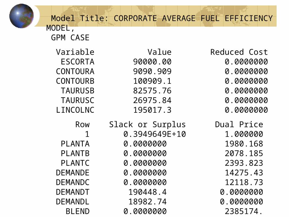
 Model Title: CORPORATE AVERAGE FUEL EFFICIENCY MODEL, GPM CASE 

Variable Value Reduced Cost ESCORTA 90000.00 0.0000000 CONTOURA 9090.909 0.0000000 CONTOURB 100909.1 0.0000000 TAURUSB 82575.76 0.0000000 TAURUSC 26975.84 0.0000000 LINCOLNC 195017.3 0.0000000 

Row Slack or Surplus Dual Price 1 0.3949649E+10 1.000000 PLANTA 0.0000000 1980.168 PLANTB 0.0000000 2078.185 PLANTC 0.0000000 2393.823 DEMANDE 0.0000000 14275.43 DEMANDC 0.0000000 12118.73 DEMANDT 190448.4 0.0000000 DEMANDL 18982.74 0.0000000 BLEND 0.0000000 2385174.

Cargo Loading - Center of Gravity Issues

C-17 Cargo Plane of Boeing McDonnell Douglas

6 5 4 3 2 1

The Plane Loading Problem

The Plane Loading Problem, details

w0 = empty weight,

d0 = distance from center of lift of empty center of gravity,

wi = weight of container i,

dj = distance of position j from center of lift,

yij = 1 if container i placed in position j,

v = tolerance for the center of gravity

deviating from center of lift.

The center of gravity is:

(w0 d0 + j dj i wi yij) / (w0 + j i wi yij).

You may wish to place a constraint on the center of gravity.What about alternate optima?

How to Compute Blended Quality

Think carefully when computing an average performance measure for a blend of things. There are three(or more) common ways of computing averages or means when one has N observations, x1, x2, . . . .xN :

Arithmetic: ( x1+ x2 . . . + xN )/N

Geometric: (x1 x2 . . . xN )^(1/N)

Harmonic: 1/[( 1/x1 + 1/x2 . . . + 1/xN )/N]

Arithmetic mean is appropriate for computing the mean return of the assets in a portfolio. The average growth of a portfolio over time, however, should be based on the geometric mean of the yearly growths. E.g., an investment that has a growth factor of 1.5 in the first year and 0.67 in the second year (e.g., a rate of return of 50% in the first year and 33% in the second year).

Data Structuring of Blending Problems

The typical blending problem has:

Several kinds of raw materials, e.g. “hydro-formed gasoline”, “reformate” gasoline, etc.

to be blending into several different finished goods, e.g. Regular, Premium, etc.

Both raw materials and finish goods share a set of qualities, e.g. volatility, vapor pressure, octane rating.

How would you (flexibly) arrange the data in a:

spreadsheet,

database or LINGO

data mining “cube”?

Pivot Tables for Converting a List to a 2-D Table

The Improv spreadsheet software in the ’90’s had an elegant capability for allowing a user to view multi-dimensional, “a data hyper cube”, data as a two dimensional table for any two desired dimensions.

MS Excel adopted this feature, implemented as the “Pivot Table” feature.

In Excel, you can think of a Pivot Table as a way of converting data in “flat file”/list form into a two dimensional table.

It is best illustrated by example(from the Blending chapter, section 10.3, in the LINGO text).

Spreadsheet Data in List Form

After: Data | PivotTable & dragging …