Childbearing Postponement, its Option Value,and the Biological Clock

David de la Croix1 Aude Pommeret2

1Universite catholique de Louvain and CEPR

2City University of Hong Kong and Universite Savoie Mont Blanc

October, 2018, Mannheim

1 / 39

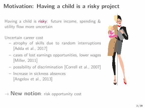
Motivation: Having a child is a risky project

Having a child is risky: future income, spending &utility flow more uncertain

Uncertain career cost– atrophy of skills due to random interruptions

[Adda et al., 2017]– cases of lost earnings opportunities, lower wages

[Miller, 2011]– possibility of discrimination [Correll et al., 2007]– Increase in sickness absences

[Angelov et al., 2013]

→ New notion: risk opportunity cost

2 / 39

But also:

Childrearing reduces women’s social network size and alters composition ofmen’s network [Munch et al., 1997]

Long-term health consequences of childbearing (urinary incontinence,weight gain, etc.)

Having a baby causes substantial declines in the average couple’srelationship [Doss et al., 2009]

Maternal mortality risk [Albanesi and Olivetti, 2016]

Pattern reinforced when children have special needs (such as visual orhearing impairment, mental retardation)

3 / 39

Research question

Literature: focus on first-order moments – effect of having a child onmean wage, on employment rate, etc.

Does not fully acknowledge the risk aspect. Stochastic models do notexplicitly make risk depend on motherhood [Sheran, 2007]

One paper focuses on exogenous income risk and procreation timing[Sommer, 2016] but risk ⊥ procreation

This paper: risk depends on procreation and it matters for optimal age atchildbearing

Question: how to model increased risk? do we find it in the data? how bigit is and does it matter for choices?

4 / 39

Idea: using option theory

Having a child is both irreversible and risky→ waiting has a value [Dixit and Pindyck, 1994]:

option value =(1) option value for receiving information+(2) pure postponement value

The riskier the project, the worthier it is to wait, even when (1)=0

The postponement value increases with risk.It interacts with fecundity (the biological clock) & assisted procreation

5 / 39

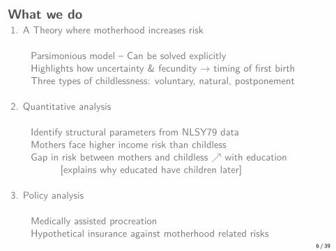
What we do1. A Theory where motherhood increases risk

Parsimonious model – Can be solved explicitlyHighlights how uncertainty & fecundity → timing of first birthThree types of childlessness: voluntary, natural, postponement

2. Quantitative analysis

Identify structural parameters from NLSY79 dataMothers face higher income risk than childlessGap in risk between mothers and childless ↗ with education

[explains why educated have children later]

3. Policy analysis

Medically assisted procreationHypothetical insurance against motherhood related risks

6 / 39

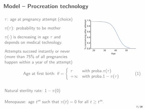
Model – Procreation technology

τ : age at pregnancy attempt (choice)

π(τ): probability to be mother

π(·) is decreasing in age τ anddepends on medical technology.

Attempts succeed instantly or never(more than 75% of all pregnancieshappen within a year of the attempt)

Age at first birth: θ ={τ with proba.π(τ)+∞ with proba.1− π(τ) (1)

Natural sterility rate: 1− π(0)

Menopause: age tm such that π(t) = 0 for all t ≥ tm.7 / 39

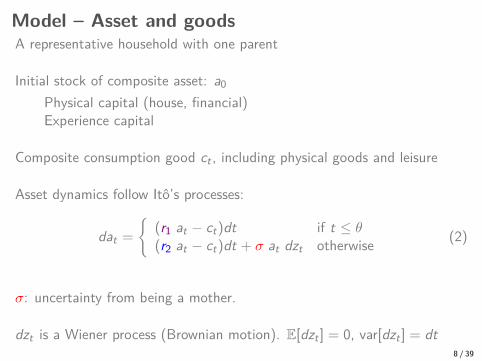
Model – Asset and goodsA representative household with one parent

Initial stock of composite asset: a0

Physical capital (house, financial)Experience capital

Composite consumption good ct , including physical goods and leisure

Asset dynamics follow Ito’s processes:

dat ={

(r1 at − ct)dt if t ≤ θ(r2 at − ct)dt + σ at dzt otherwise (2)

σ: uncertainty from being a mother.

dzt is a Wiener process (Brownian motion). E[dzt ] = 0, var[dzt ] = dt8 / 39

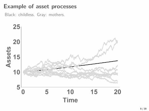
Example of asset processesBlack: childless. Gray: mothers.

9 / 39

Model – PreferencesUtility:

∞∫0

u(ct) e−ρtdt + e−ρθω

ω is the lump-sum utility (joy) of having children,and ρ is the psychological discount rate

CRRA utility function:

u(ct) = c1−εt

1− εε > 1: the coefficient of relative risk aversion

Choices:

arg maxct ,at ,τ

E

∞∫0

u(ct) e−ρtdt + e−ρθω

subject to (1), (2).

10 / 39

Model – Methodology

The problem has to be solved recursively:

[A] We first consider the post-birth program, once the pregnancy attempthas proven successful. (Stochastic optimal control [Turnovsky, 2000])Consumption follows

ct = qat , ∀t ≥ τ

with the propensity to consume out of wealth given by

q =ρ− (1− ε)

(r2 − ε

2σ2)

ε

This delivers a utility W2(aτ ) at a date τ with probability π(τ):

W2(aτ ) = q−ε a1−ετ

1− ε + ω.

11 / 39

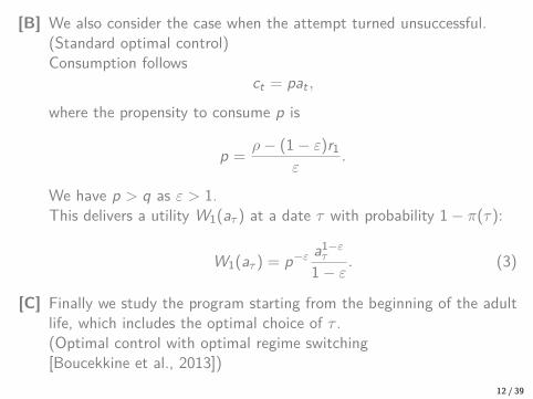
[B] We also consider the case when the attempt turned unsuccessful.(Standard optimal control)Consumption follows

ct = pat ,

where the propensity to consume p is

p = ρ− (1− ε)r1ε

.

We have p > q as ε > 1.This delivers a utility W1(aτ ) at a date τ with probability 1− π(τ):

W1(aτ ) = p−ε a1−ετ

1− ε. (3)

[C] Finally we study the program starting from the beginning of the adultlife, which includes the optimal choice of τ .(Optimal control with optimal regime switching[Boucekkine et al., 2013])

12 / 39

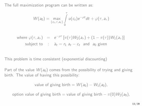
The full maximization program can be written as:

W (a0) = max{ct ,τ,at}

τ∫0

u(ct)e−ρtdt + ϕ(τ, aτ )

where ϕ(τ, aτ ) = e−ρτ [π(τ)W2(aτ ) + (1− π(τ))W1(aτ )]subject to : at = r1 at − ct and a0 given

This problem is time consistent (exponential discounting)

Part of the value W (a0) comes from the possibility of trying and givingbirth. The value of having this possibility:

value of giving birth = W (a0)−W1(a0),

option value of giving birth = value of giving birth− π(0)W2(a0),

13 / 39

Solving the full maximization program

Define the following Hamiltonian:

H(c, a, µ) = U(c)e−ρt + µ (r1 a − c)

The value-function W (a0) in terms of the Hamiltonian H(·):

W (a0) =τ∫

0

(H(ct , at , µt)− µt at) dt + ϕ(τ, aτ )

14 / 39

First-Order Conditions

∂H(ct , at , µt)∂ct

= 0,

∂H(ct , at , µt)∂at

+ µt = 0,

H(cτ , aτ , µτ ) + ∂ϕ(τ, aτ )∂τ

= 0,

∂ϕ(τ, aτ )∂aτ

− µτ = 0.

The first two conditions are the standard Pontryagin conditions.

The third one equalizes the marginal benefit of waiting to the marginal costof waiting.

The last one is a continuity condition.

These conditions are necessary but not sufficient for an interior maximum.

15 / 39

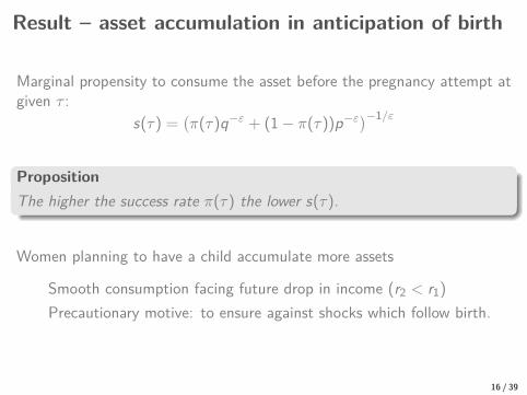
Result – asset accumulation in anticipation of birth

Marginal propensity to consume the asset before the pregnancy attempt atgiven τ :

s(τ) =(π(τ)q−ε + (1− π(τ))p−ε

)−1/ε

PropositionThe higher the success rate π(τ) the lower s(τ).

Women planning to have a child accumulate more assets

Smooth consumption facing future drop in income (r2 < r1)Precautionary motive: to ensure against shocks which follow birth.

16 / 39

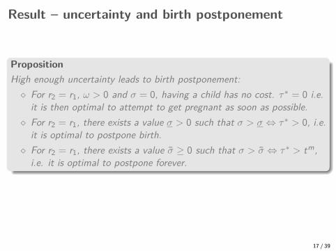
Result – uncertainty and birth postponement

PropositionHigh enough uncertainty leads to birth postponement:� For r2 = r1, ω > 0 and σ = 0, having a child has no cost. τ∗ = 0 i.e.

it is then optimal to attempt to get pregnant as soon as possible.� For r2 = r1, there exists a value σ > 0 such that σ > σ ⇔ τ∗ > 0, i.e.

it is optimal to postpone birth.� For r2 = r1, there exists a value σ ≥ 0 such that σ > σ ⇔ τ∗ > tm,

i.e. it is optimal to postpone forever.

17 / 39

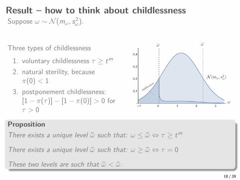
Result – how to think about childlessnessSuppose ω ∼ N (mω, s2

ω).

Three types of childlessness

1. voluntary childlessness τ ≥ tm

2. natural sterility, becauseπ(0) < 1

3. postponement childlessness:[1− π(τ)]− [1− π(0)] > 0 forτ > 0

ω ω

N (mω, s2ω)

ω

childlessness

PropositionThere exists a unique level ω such that: ω ≤ ω ⇔ τ ≥ tm

There exists a unique level ω such that: ω ≥ ω ⇔ τ = 0

These two levels are such that ω < ω.18 / 39

Let us move now tothe quantitative analysis

19 / 39

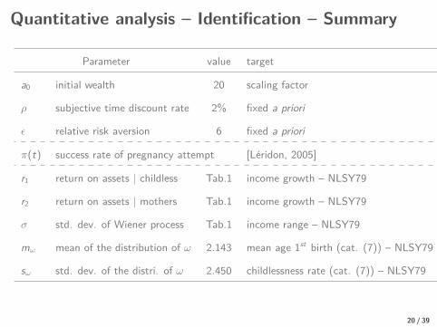
Quantitative analysis – Identification – Summary

Parameter value target

a0 initial wealth 20 scaling factor

ρ subjective time discount rate 2% fixed a priori

ε relative risk aversion 6 fixed a priori

π(t) success rate of pregnancy attempt [Leridon, 2005]

r1 return on assets | childless Tab.1 income growth – NLSY79

r2 return on assets | mothers Tab.1 income growth – NLSY79

σ std. dev. of Wiener process Tab.1 income range – NLSY79

mω mean of the distribution of ω 2.143 mean age 1st birth (cat. (7)) – NLSY79

sω std. dev. of the distri. of ω 2.450 childlessness rate (cat. (7)) – NLSY79

20 / 39

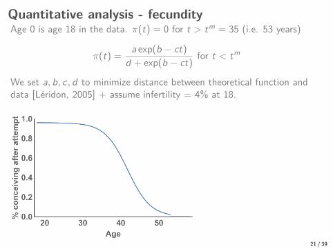
Quantitative analysis - fecundityAge 0 is age 18 in the data. π(t) = 0 for t > tm = 35 (i.e. 53 years)

π(t) = a exp(b − ct)d + exp(b − ct) for t < tm

We set a, b, c, d to minimize distance between theoretical function anddata [Leridon, 2005] + assume infertility = 4% at 18.

21 / 39

Quantitative analysis - NLSY79

Longitudinal project that follows the lives of a sample of American youthborn between 1957-64.

The cohort originally included 12,686 respondents ages 14-22 when firstinterviewed in 1979.

Data are now available from Round 1 (1979 survey year) to Round 25(2012 survey year).

We take all women with positive income, consider their income from age39-45.

22 / 39

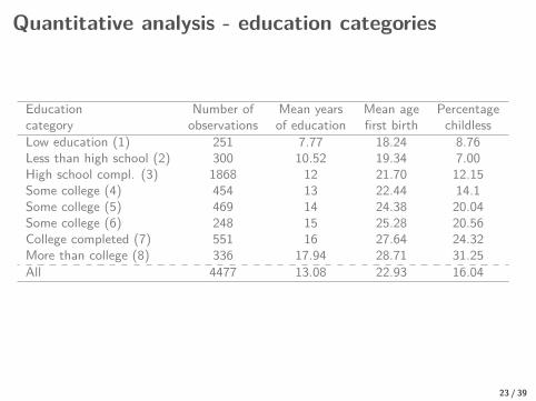
Quantitative analysis - education categories

Education Number of Mean years Mean age Percentagecategory observations of education first birth childlessLow education (1) 251 7.77 18.24 8.76Less than high school (2) 300 10.52 19.34 7.00High school compl. (3) 1868 12 21.70 12.15Some college (4) 454 13 22.44 14.1Some college (5) 469 14 24.38 20.04Some college (6) 248 15 25.28 20.56College completed (7) 551 16 27.64 24.32More than college (8) 336 17.94 28.71 31.25All 4477 13.08 22.93 16.04

23 / 39

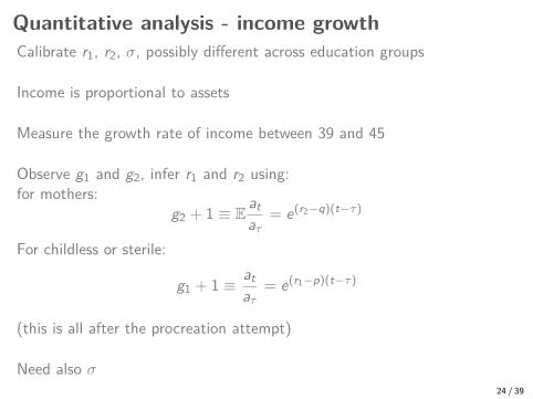
Quantitative analysis - income growthCalibrate r1, r2, σ, possibly different across education groups

Income is proportional to assets

Measure the growth rate of income between 39 and 45

Observe g1 and g2, infer r1 and r2 using:for mothers:

g2 + 1 ≡ Eataτ

= e(r2−q)(t−τ)

For childless or sterile:

g1 + 1 ≡ ataτ

= e(r1−p)(t−τ)

(this is all after the procreation attempt)

Need also σ24 / 39

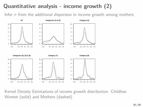
Quantitative analysis - income growth (2)Infer σ from the additional dispersion in income growth among mothers

−0.3 −0.1 0.0 0.1 0.2 0.3

02

46

810

All

−0.3 −0.1 0.0 0.1 0.2 0.3

02

46

810

Categories (1) & (2)

−0.3 −0.1 0.0 0.1 0.2 0.3

02

46

810

Category (3)

−0.3 −0.1 0.0 0.1 0.2 0.3

02

46

810

Categories (4), (5) & (6)

−0.3 −0.1 0.0 0.1 0.2 0.3

02

46

810

Category (7)

−0.3 −0.1 0.0 0.1 0.2 0.3

02

46

810

Category (8)

Kernel Density Estimations of income growth distribution. ChildlessWomen (solid) and Mothers (dashed)

25 / 39

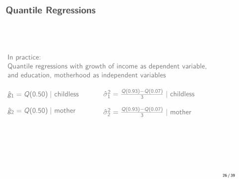
Quantile Regressions

In practice:Quantile regressions with growth of income as dependent variable,and education, motherhood as independent variables

g1 = Q(0.50) | childless

g2 = Q(0.50) | mother

σ21 = Q(0.93)−Q(0.07)

3 | childless

σ22 = Q(0.93)−Q(0.07)

3 | mother

26 / 39

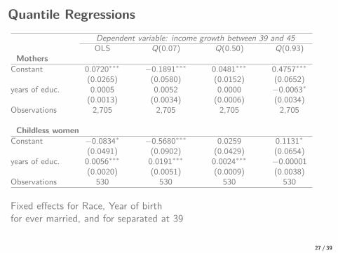
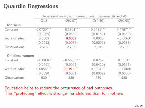
Quantile RegressionsDependent variable: income growth between 39 and 45OLS Q(0.07) Q(0.50) Q(0.93)

MothersConstant 0.0720∗∗∗ −0.1891∗∗∗ 0.0481∗∗∗ 0.4757∗∗∗

(0.0265) (0.0580) (0.0152) (0.0652)years of educ. 0.0005 0.0052 0.0000 −0.0063∗

(0.0013) (0.0034) (0.0006) (0.0034)Observations 2,705 2,705 2,705 2,705

Childless womenConstant −0.0834∗ −0.5680∗∗∗ 0.0259 0.1131∗

(0.0491) (0.0902) (0.0429) (0.0654)years of educ. 0.0056∗∗∗ 0.0191∗∗∗ 0.0024∗∗∗ −0.00001

(0.0020) (0.0051) (0.0009) (0.0038)Observations 530 530 530 530

Fixed effects for Race, Year of birthfor ever married, and for separated at 39

27 / 39

Quantile RegressionsDependent variable: income growth between 39 and 45OLS Q(0.07) Q(0.50) Q(0.93)

MothersConstant 0.0720∗∗∗ −0.1891∗∗∗ 0.0481∗∗∗ 0.4757∗∗∗

(0.0265) (0.0580) (0.0152) (0.0652)years of educ. 0.0005 0.0052 0.0000 −0.0063∗

(0.0013) (0.0034) (0.0006) (0.0034)Observations 2,705 2,705 2,705 2,705

Childless womenConstant −0.0834∗ −0.5680∗∗∗ 0.0259 0.1131∗

(0.0491) (0.0902) (0.0429) (0.0654)years of educ. 0.0056∗∗∗ 0.0191∗∗∗ 0.0024∗∗∗ −0.00001

(0.0020) (0.0051) (0.0009) (0.0038)Observations 530 530 530 530

Education helps to reduce the occurrence of bad outcomes.This “protecting” effect is stronger for childless than for mothers

28 / 39

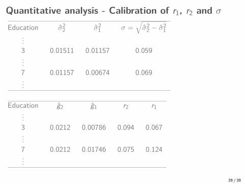
Quantitative analysis - Calibration of r1, r2 and σ

Education σ22 σ2

1 σ =√σ2

2 − σ21

...3 0.01511 0.01157 0.059...7 0.01157 0.00674 0.069...

Education g2 g1 r2 r1...3 0.0212 0.00786 0.094 0.067...7 0.0212 0.01746 0.075 0.124...

29 / 39

Quantitative analysis - Calibration of ω

Exact identification: Parameters of the normal distribution functionN (mω, s2

ω) set to match the mean age at first birth and the childlessnessrate of the education category 7 ( 27.64 years and 24.32%).

It yields mω = 2.143 and sω = 2.450

30 / 39

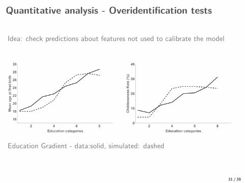
Quantitative analysis - Overidentification tests

Idea: check predictions about features not used to calibrate the model

Education Gradient - data:solid, simulated: dashed

31 / 39

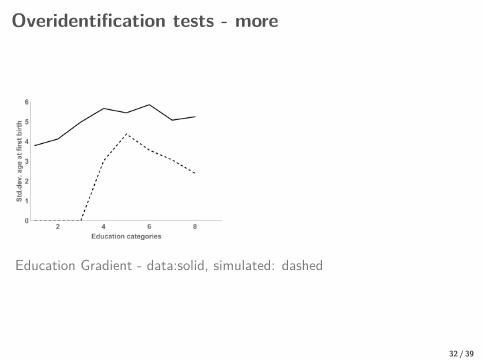
Overidentification tests - more

Education Gradient - data:solid, simulated: dashed

32 / 39

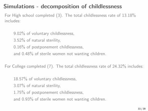
Simulations - decomposition of childlessnessFor High school completed (3). The total childlessness rate of 13.18%includes:

9.02% of voluntary childlessness,3.52% of natural sterility,0.16% of postponement childlessness,and 0.48% of sterile women not wanting children.

For College completed (7). The total childlessness rate of 24.32% includes:

18.57% of voluntary childlessness,3.07% of natural sterility,1.75% of postponement childlessness,and 0.93% of sterile women not wanting children.

33 / 39

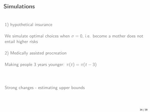
Simulations

1) hypothetical insurance

We simulate optimal choices when σ = 0, i.e. become a mother does notentail higher risks

2) Medically assisted procreation

Making people 3 years younger: π(t) = π(t − 3)

Strong changes - estimating upper bounds

34 / 39

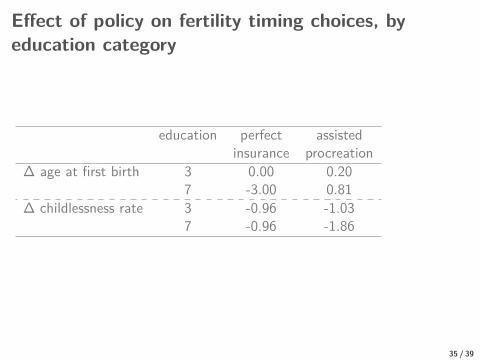
Effect of policy on fertility timing choices, byeducation category

education perfect assistedinsurance procreation

∆ age at first birth 3 0.00 0.207 -3.00 0.81

∆ childlessness rate 3 -0.96 -1.037 -0.96 -1.86

35 / 39

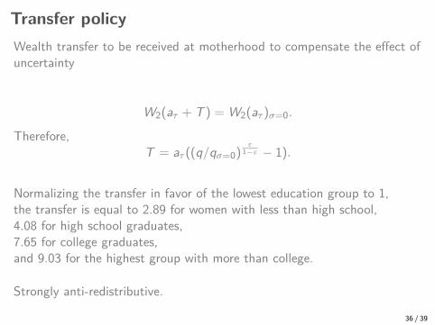
Transfer policyWealth transfer to be received at motherhood to compensate the effect ofuncertainty

W2(aτ + T ) = W2(aτ )σ=0.

Therefore,T = aτ ((q/qσ=0)

ε1−ε − 1).

Normalizing the transfer in favor of the lowest education group to 1,the transfer is equal to 2.89 for women with less than high school,4.08 for high school graduates,7.65 for college graduates,and 9.03 for the highest group with more than college.

Strongly anti-redistributive.

36 / 39

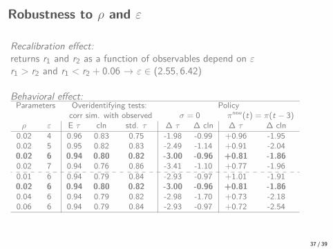
Robustness to ρ and ε

Recalibration effect:returns r1 and r2 as a function of observables depend on εr1 > r2 and r1 < r2 + 0.06 → ε ∈ (2.55, 6.42)

Behavioral effect:Parameters Overidentifying tests: Policy

corr sim. with observed σ = 0 πnew(t) = π(t − 3)ρ ε E τ cln std. τ ∆ τ ∆ cln ∆ τ ∆ cln

0.02 4 0.96 0.83 0.75 -1.98 -0.99 +0.96 -1.950.02 5 0.95 0.82 0.83 -2.49 -1.14 +0.91 -2.040.02 6 0.94 0.80 0.82 -3.00 -0.96 +0.81 -1.860.02 7 0.94 0.76 0.86 -3.41 -1.10 +0.77 -1.960.01 6 0.94 0.79 0.84 -2.93 -0.97 +1.01 -1.910.02 6 0.94 0.80 0.82 -3.00 -0.96 +0.81 -1.860.04 6 0.94 0.79 0.82 -2.98 -1.70 +0.73 -2.180.06 6 0.94 0.79 0.84 -2.93 -0.97 +0.72 -2.54

37 / 39

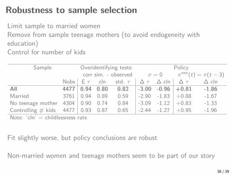
Robustness to sample selectionLimit sample to married womenRemove from sample teenage mothers (to avoid endogeneity witheducation)Control for number of kids

Sample Overidentifying tests: Policycorr sim. - observed σ = 0 πnew(t) = π(t − 3)

Nobs E τ cln std. τ ∆ τ ∆ cln ∆ τ ∆ clnAll 4477 0.94 0.80 0.82 -3.00 -0.96 +0.81 -1.86Married 3761 0.94 0.89 0.59 -2.90 -1.83 +0.88 -1.67No teenage mother 4304 0.90 0.74 0.84 -3.09 -1.12 +0.83 -1.33Controlling # kids 4477 0.93 0.87 0.65 -2.44 -1.27 +0.95 -1.96Note: ‘cln’ = childlessness rate

Fit slightly worse, but policy conclusions are robust

Non-married women and teenage mothers seem to be part of our story

38 / 39

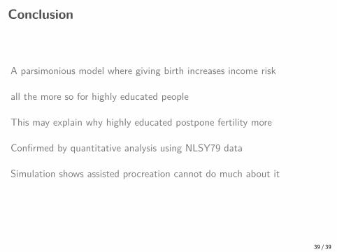
Conclusion

A parsimonious model where giving birth increases income risk

all the more so for highly educated people

This may explain why highly educated postpone fertility more

Confirmed by quantitative analysis using NLSY79 data

Simulation shows assisted procreation cannot do much about it

39 / 39

Adda, J., Dustmann, C., and Stevens, K. (2017).The Career Costs of Children.Journal of Political Economy, 125(2):293–337.

Albanesi, S. and Olivetti, C. (2014).Maternal health and the baby boom.Quantitative Economics, 5(2):225–269.

Albanesi, S. and Olivetti, C. (2016).Gender roles and medical progress.Journal of Political Economy, 124(3):650–695.

Angelov, N., Johansson, P., and Lindahl, E. (2013).Gender Differences in Sickness Absence and the Gender Division of FamilyResponsibilities.IZA Discussion Papers 7379, Institute for the Study of Labor (IZA).

Boucekkine, R., Pommeret, A., and Prieur, F. (2013).Optimal regime switching and threshold effects.Journal of Economic Dynamics and Control, 37(12):2979–2997.

Correll, S. J., Benard, S., and Paik, I. (2007).Getting a job: Is there a motherhood penalty?

39 / 39

American Journal of Sociology, 112(5):1297–1338.

Dixit, A. and Pindyck, R. (1994).Investment under Uncertainty.Princeton University Press, Princeton.

Doss, B., Rhoades, G. K., Stanley, S. M., and Markman, H. J. (2009).The effect of the transition to parenthood on relationship quality: An 8-yearprospective study.Journal of Personality and Social Psychology, 96(3):601–619.

Leridon, H. (2005).How effective is assisted reproduction technology? a model assessment.Revue d’Epidemiologie et de Sante Publique, 53:119–127.

Miller, A. (2011).The effects of motherhood timing on career path.Journal of Population Economics, 24(3):1071–1100.

Munch, A., McPherson, J. M., and Smith-Lovin, L. (1997).Gender, children, and social contact: The effects of childrearing for men andwomen.American Sociological Review, 62(4):509–520.

39 / 39

Sheran, M. (2007).The career and family choices of women: A dynamic analysis of labor forceparticipation, schooling, marriage, and fertility decisions.Review of Economic Dynamics, 10:367–399.

Sommer, K. (2016).Fertility choice in a life cycle model with idiosyncratic uninsurable earnings risk.Journal of Monetary Economics, 83:27 – 38.

Turnovsky, S. J. (2000).Methods of macroeconomic dynamics.Mit Press, Cambridge MA.

39 / 39