Chetan Kapoor Dissertation
613
Copyright by Chetan Kapoor 1996
-
Upload
ana-hanami -
Category
Documents
-
view
226 -
download
0
Transcript of Chetan Kapoor Dissertation

8/3/2019 Chetan Kapoor Dissertation
http://slidepdf.com/reader/full/chetan-kapoor-dissertation 1/612
Copyright
by
Chetan Kapoor
1996
8/3/2019 Chetan Kapoor Dissertation
http://slidepdf.com/reader/full/chetan-kapoor-dissertation 2/612
A Reusable Operational Software Architecture for
Advanced Robotics
by
Chetan Kapoor, M.S.
Dissertation
Presented to the Faculty of the Graduate School of
the University of Texas at Austin
in Partial Fulfillment
of the Requirements
for the Degree of
Doctor of Philosophy
The University of Texas at Austin
December, 1996
8/3/2019 Chetan Kapoor Dissertation
http://slidepdf.com/reader/full/chetan-kapoor-dissertation 3/612
A Reusable Operational Software Architecture for
Advanced Robotics
Approved by
Dissertation Committee:

8/3/2019 Chetan Kapoor Dissertation
http://slidepdf.com/reader/full/chetan-kapoor-dissertation 4/612
To my Parents
Subhash Kapoor and Rewa Kapoor
8/3/2019 Chetan Kapoor Dissertation
http://slidepdf.com/reader/full/chetan-kapoor-dissertation 5/612
v
Acknowledgments
This work was partially funded by the U.S. Department of Energy (Grant
No. DE-FG01-94EW37966), and NASA (Grant No. NAG 9-809). This research
would not have been possible without the constant guidance, help, and support of
Dr. Delbert Tesar, my committee chairman and academic advisor. I would also
like to thank my committee members Dr. Rich Hooper, Dr. James Browne, Dr.
S.V. Sreenivasan, Dr. Dan Cox, and Dr. Richard Crawford, who’s time and help
is very much appreciated.
I would also like to thank Kevin Rackers for testing the software andCarsten Puls for offering useful suggestions regarding the writing of this report.
Thanks are due to Murat Cetin, Mitch Pryor, Troy Harden, Jorge Ruiz, Chris
Cocca, Andy Legoullen, and Dr. Rich Hooper for evaluating this research.
Finally, I owe a lot to my family and friends who have brought me to this
denouement. This research would be incomplete without a mention of their
sacrifice and support.

8/3/2019 Chetan Kapoor Dissertation
http://slidepdf.com/reader/full/chetan-kapoor-dissertation 6/612
vi
A Reusable Operational Software Architecture for
Advanced Robotics
Publication No. ________________
Chetan Kapoor, Ph.D.
The University of Texas at Austin, 1996
Supervisor: Delbert Tesar
Robotic software can be broadly categorized into two levels. The first is
the actuator control software. The other level is the system control software.
Three layers further comprise the system control software. The top-most is the
man-machine interface. The lowest is the real-time control layer. The middlelayer is known as the operational software layer.
Current industrial robots are monolithic six degrees-of-freedom
manipulators that have minimal operational software requirements. On the other
hand, advanced robots are based on modularity, redundancy, fault-tolerance, and
performance. The operational software layer for these robots should be general
and reconfigurable, and should support kinematics, dynamics, deflection
modeling, performance criteria, fault-tolerance, and condition-based maintenance.
The development of a reusable and general architecture for the operational
software layer is the prime goal of this research. This includes:
• requirements generation for an advanced robotic software system,
8/3/2019 Chetan Kapoor Dissertation
http://slidepdf.com/reader/full/chetan-kapoor-dissertation 7/612
vii
• the selection of a development, execution, and test environment,
•
the development of a reusable software architecture to support OperationalSoftware Components for Advanced Robots (OSCAR),
• the development of applications to demonstrate OSCAR in simulation on a
wide variety of robots and in real-time on a seventeen degrees-of-freedom
dual-arm manipulator,
• the design and development of experiments to validate the advantages of
OSCAR,
• development and demonstration of a real-time formulation of the direct-search
generalized inverse kinematics scheme.
The development of OSCAR is based on object-oriented design. Object-
oriented design professes the development of software components that are
extensible and have standardized interfaces. The application of this philosophy
led to the break-down of the advanced robotics domain into sub-domains. An
analysis of these sub-domains lead to the identification of components that made
up the sub-domain. A detailed analysis and design of these components then
followed.
Applications and experimentation validated the effectiveness of this
software architecture. Achieved goals of this software architecture were
demonstrated by the applications. The experiments demonstrated that OSCAR
provided a 30% improvement in its ‘ease of use’ and an approximately 200%
reduction in program development time as compared to the other robotic software
in use at the Robotics Research Group.
The real-time formulation of the direct-search inverse kinematics
technique showed a 170-times performance improvement when used on a seven
degrees-of-freedom robot.
8/3/2019 Chetan Kapoor Dissertation
http://slidepdf.com/reader/full/chetan-kapoor-dissertation 8/612
viii
Table of Contents
LIST OF TABLES ................................................................................................................. .... xvii
LIST OF FIGURES ................................................................................................................ ......xx
NOMENCLATURE...................................................................................................................xxiv
CHAPTER ONE INTRODUCTION............................................................................................1
1.1. THE THREE LAYERS OF A ROBOTIC SOFTWARE SYSTEM........................................................21.2. RESEARCH OBJECTIVES .........................................................................................................41.3. MODULAR ROBOTICS.............................................................................................................61.4. ROBOT CONTROL ...................................................................................................................71.5. GENERALIZED KINEMATICS ...................................................................................................81.6. GENERALIZED DYNAMICS ......................................................................................................91.7. DEFLECTION MODELING ......................................................................................................101.8. FAULT-TOLERANCE .............................................................................................................111.9. DECISION MAKING...............................................................................................................121.10. OVERVIEW .........................................................................................................................14
CHAPTER TWO LITERATURE REVIEW.............................................................................17
2.1. INTRODUCTION ....................................................................................................................172.2. MECHANICAL HARDWARE ...................................................................................................20
2.2.1. Modularity and Reconfigurability ...............................................................................21
2.2.2. Redundancy and Fault-Tolerance ...............................................................................25
2.2.3. Precision......................................................................................................................26
2.2.4. Maintainability ............................................................................................................27
2.3. COMPUTER HARDWARE .......................................................................................................292.3.1. Servo-Level Hardware.................................................................................................30
2.3.1.1. Centralized Control ............................................................................................................312.3.1.2. Distributed Control .............................................................................................................32
2.3.2. System Controller Hardware.......................................................................................33
2.3.3. Computer Bus ..............................................................................................................35
2.4. SOFTWARE ...........................................................................................................................372.5. SOFTWARE TECHNOLOGY ....................................................................................................40
2.5.1. Software Design...........................................................................................................412.5.1.1. Structured Design...............................................................................................................412.5.1.2. Object-Oriented Design......................................................................................................42
2.5.1.2.1. Classes........................................................................................................................ 432.5.1.2.2. Data Abstraction.........................................................................................................462.5.1.2.3. Inheritance..................................................................................................................47
2.5.1.2.4. Polymorphism ............................................................................................................492.5.1.2.5. Dynamic Binding .......................................................................................................492.5.1.3. Object Oriented Support for Good Design .........................................................................50
2.5.2. Real-Time Software .....................................................................................................532.5.2.1. Ad Hoc Approach...............................................................................................................532.5.2.2. Multitasking Approach.......................................................................................................552.5.2.3. Real-Time Operating Systems ............................................................................................56
2.6. ROBOTIC SOFTWARE SYSTEMS ............................................................................................58
8/3/2019 Chetan Kapoor Dissertation
http://slidepdf.com/reader/full/chetan-kapoor-dissertation 9/612
ix
2.6.1. Man-Machine Interface ............ ............ ............ ............ ............. ............ ............ ..........58
2.6.2. Operational Software ..................................................................................................592.6.2.1. RCCL (Robot Control C Libraries) ....................................................................................602.6.2.2. Robot Independent Programming Environment (RIPE).....................................................612.6.2.3. Generic Intelligent System Control (GISC)........................................................................612.6.2.4. Sequential Modular Architecture for Robotics and Teleoperation .....................................622.6.2.5. Control Shell ......................................................................................................................632.6.2.6. Robot Shell.........................................................................................................................642.6.2.7. Design Automation.............................................................................................................642.6.2.8. Various Object-Oriented Robotic Environments................................................................662.6.2.9. Summary of the Operational Software Literature Review..................................................68
2.6.3. Real-time Layer ...........................................................................................................70
2.7. IMPACT OF ADVANCEMENT IN COMPUTER TECHNOLOGY....................................................712.8. DESIRED CHARACTERISTICS OF THE SOFTWARE SYSTEM .....................................................722.9. GENERALIZED KINEMATICS .................................................................................................75
2.9.1. Direct-Search Formulation .........................................................................................76
2.10. SUMMARY..........................................................................................................................77CHAPTER THREE PERFORMANCE-BASED HYBRID GENERALIZED INVERSE .....80
3.1. INTRODUCTION ....................................................................................................................803.2. INVERSE KINEMATICS ..........................................................................................................803.3. DIRECT SEARCH TECHNIQUE ...............................................................................................83
3.3.1. Strengths......................................................................................................................89
3.3.2. Weaknesses..................................................................................................................89
3.4. HYBRID FORMULATION........................................................................................................903.4.1. Generalized Inverse Scheme........................................................................................92
3.4.2. Options Ranking..........................................................................................................96
3.5. EXAMPLE OF HYBRID GENERALIZED INVERSE ...................................................................1013.5.1. Example Performance Criteria..................................................................................102
3.5.2. Example Results.........................................................................................................1033.5.3. Performance Comparison with Hooper’s [1994] Scheme ........................................108
3.6. SUMMARY..........................................................................................................................110
CHAPTER FOUR DEVELOPMENT, EXECUTION, AND TEST ENVIRONMENT.......111
4.1. DEVELOPMENT AND EXECUTION ENVIRONMENT TYPES ....................................................1124.1.1. Self-Hosted Systems...................................................................................................112
4.1.2. Cross-Development Systems......................................................................................114
4.2. DEVELOPMENT ENVIRONMENT SELECTION........................................................................1154.2.1. Software Design Methodology...................................................................................116
4.2.2. Language Selection ...................................................................................................117
4.2.3. Operating System Selection .......................................................................................119
4.3. EXECUTION ENVIRONMENT SELECTION .............................................................................121
4.3.1. Operating System Selection ............ ............ ............ ............ ............. ............ ............ ..1224.3.2. Execution Computer Hardware.................................................................................1254.3.2.1. Processor ............................................................................................................. .............1264.3.2.2. Bus Type...........................................................................................................................128
4.4. SUMMARY OF THE SELECTED ENVIRONMENT ....................................................................1314.5. TEST ENVIRONMENT CHARACTERISTICS............................................................................1334.6. HARDWARE DESCRIPTION ..................................................................................................143
8/3/2019 Chetan Kapoor Dissertation
http://slidepdf.com/reader/full/chetan-kapoor-dissertation 10/612
x
4.7. ORGANIZATIONAL AND MANAGERIAL ISSUES ....................................................................1544.8. SUMMARY..........................................................................................................................155
1. INTRODUCTION .................................................................................................................1
1.1. THE THREE LAYERS OF A ROBOTIC SOFTWARE SYSTEM .....................................................21.2. RESEARCH OBJECTIVES .......................................................................................................41.3. MODULAR ROBOTICS...........................................................................................................61.4. ROBOT CONTROL.................................................................................................................71.5. GENERALIZED KINEMATICS .................................................................................................81.6. GENERALIZED DYNAMICS ...................................................................................................91.7. DEFLECTION MODELING ....................................................................................................101.8. FAULT-TOLERANCE ...........................................................................................................111.9. DECISION MAKING.............................................................................................................121.10. OVERVIEW....................................................................................................................14
2. LITERATURE REVIEW ...................................................................................................17
2.1. INTRODUCTION..................................................................................................................172.2. MECHANICAL HARDWARE.................................................................................................20
2.2.1. Modularity and Reconfigurability...........................................................................21
2.2.2. Redundancy and Fault-Tolerance...........................................................................25
2.2.3. Precision .................................................................................................................26
2.2.4. Maintainability........................................................................................................27
2.3. COMPUTER HARDWARE.....................................................................................................292.3.1. Servo-Level Hardware ............................................................................................30
2.3.1.1. ..................................................................................................Centralized Control31
2.3.1.2. ..................................................................................................Distributed Control32
2.3.2. System Controller Hardware...................................................................................332.3.3. Computer Bus..........................................................................................................35
2.4. SOFTWARE.........................................................................................................................372.5. SOFTWARE TECHNOLOGY..................................................................................................40
2.5.1. Software Design ......................................................................................................412.5.1.1. .................................................................................................... Structured Design41
2.5.1.2. ........................................................................................... Object-Oriented Design42
2.5.1.2.1..............................................................................................................Classes43
2.5.1.2.2............................................................................................... Data Abstraction46
2.5.1.2.3........................................................................................................ Inheritance47
2.5.1.2.4...................................................................................................Polymorphism49
2.5.1.2.5..............................................................................................Dynamic Binding49
2.5.1.3. .............................................................. Object Oriented Support for Good Design50
2.5.2. Real-Time Software.................................................................................................532.5.2.1. ....................................................................................................Ad Hoc Approach53
2.5.2.2. ............................................................................................ Multitasking Approach55
8/3/2019 Chetan Kapoor Dissertation
http://slidepdf.com/reader/full/chetan-kapoor-dissertation 11/612
xi
2.5.2.3. ................................................................................. Real-Time Operating Systems56
2.6. ROBOTIC SOFTWARE SYSTEMS ..........................................................................................58
2.6.1. Man-Machine Interface...........................................................................................582.6.2. Operational Software ..............................................................................................59
2.6.2.1. ......................................................................... RCCL (Robot Control C Libraries)60
2.6.2.2. .......................................... Robot Independent Programming Environment (RIPE)61
2.6.2.3. ............................................................. Generic Intelligent System Control (GISC)61
2.6.2.4. .......................... Sequential Modular Architecture for Robotics and Teleoperation62
2.6.2.5. ............................................................................................................Control She ll63
2.6.2.6. .............................................................................................................. Robot Shell 64
2.6.2.7. ..................................................................................................Design Automation64
2.6.2.8......................................................Various Object-Oriented Robotic Environments66
2.6.2.9. ....................................... Summary of the Operational Software Literature Review68
2.6.3. Real-time Layer.......................................................................................................70
2.7. IMPACT OF ADVANCEMENT IN COMPUTER TECHNOLOGY..................................................712.8. DESIRED CHARACTERISTICS OF THE SOFTWARE SYSTEM ..................................................722.9. GENERALIZED KINEMATICS ...............................................................................................75
2.9.1. Direct-Search Formulation.....................................................................................76
2.10. SUMMARY ....................................................................................................................77
3. PERFORMANCE-BASED HYBRID GENERALIZED INVERSE................................80
3.1. INTRODUCTION..................................................................................................................803.2. INVERSE KINEMATICS........................................................................................................803.3. DIRECT SEARCH TECHNIQUE .............................................................................................83
3.3.1. Strengths..................................................................................................................89
3.3.2. Weaknesses..............................................................................................................893.4. HYBRID FORMULATION .....................................................................................................90
3.4.1. Generalized Inverse Scheme ...................................................................................92
3.4.2. Options Ranking......................................................................................................96
3.5. EXAMPLE OF HYBRID GENERALIZED INVERSE.................................................................1013.5.1. Example Performance Criteria .............................................................................102
3.5.2. Example Results ....................................................................................................103
3.5.3. Performance Comparison with Hooper’s [1994] Scheme....................................108
3.6. SUMMARY .......................................................................................................................110
4. DEVELOPMENT, EXECUTION, AND TEST ENVIRONMENT...............................111
4.1. DEVELOPMENT AND EXECUTION ENVIRONMENT TYPES..................................................1124.1.1. Self-Hosted Systems ..............................................................................................112
4.1.2. Cross-Development Systems..................................................................................1144.2. DEVELOPMENT ENVIRONMENT SELECTION .....................................................................115
4.2.1. Software Design Methodology ..............................................................................116
4.2.2. Language Selection ...............................................................................................117
4.2.3. Operating System Selection...................................................................................119
4.3. EXECUTION ENVIRONMENT SELECTION ...........................................................................1214.3.1. Operating System Selection...................................................................................122
8/3/2019 Chetan Kapoor Dissertation
http://slidepdf.com/reader/full/chetan-kapoor-dissertation 12/612
xii
4.3.2. Execution Computer Hardware ............................................................................1254.3.2.1...................................................................................................................Processor126
4.3.2.2. ..................................................................................................................Bus Type128
4.4. SUMMARY OF THE SELECTED ENVIRONMENT ..................................................................1314.5. TEST ENVIRONMENT CHARACTERISTICS..........................................................................1334.6. HARDWARE DESCRIPTION ...............................................................................................1434.7. ORGANIZATIONAL AND MANAGERIAL ISSUES ..................................................................1544.8. SUMMARY .......................................................................................................................155
8/3/2019 Chetan Kapoor Dissertation
http://slidepdf.com/reader/full/chetan-kapoor-dissertation 13/612
xiii
APPENDIX A SOFTWARE DEVELOPMENT GUIDELINES............................................369
A.1. SOFTWARE DESIGN PHILOSOPHY.......................................................................................369
A.2. HOW DO WE ACHIEVE OUR DESIGN GOALS? .......................................................................370A.3. THE DESIGN PROCESS .......................................................................................................371A.4. TRADITIONAL ENGINEERING DESIGN.................................................................................372
A.4.1. What is Design? ........................................................................................................372
A.4.2. What are the qualities of a good designer?...............................................................372
A.4.3. Summary of the Design Process................................................................................372
A.4.4. Critical Path Analysis ...............................................................................................373
A.5. SOFTWARE DESIGN PROCESS ............................................................................................373 A.5.1. Requirement Analysis................................................................................................373
A.5.2. Domain Analysis .......................................................................................................373
A.5.3. System Design ...........................................................................................................374
A.6. PROGRAMMING GUIDELINES .............................................................................................375A.7. EXAMPLE ..........................................................................................................................376
A.7.1. File Vector.hpp..........................................................................................................376 A.7.2. File Vector.ipp ..........................................................................................................378
A.7.3. File Vector.cpp..........................................................................................................381
APPENDIX B OSCAR CLASS LIBRARY REFERENCE....................................................384
B.1. BASE ABSTRACTIONS........................................................................................................384 B.1.1. class RRBase.............................................................................................................384
B.2. MATHEMATICAL ABSTRACTIONS.......................................................................................386 B.2.1. class RRVector : public RRBase ..............................................................................386
B.2.2. Class RRVector3 : public RRVector........ .......... ........... .......... ........... .......... ........... ..391
B.2.3. Class RRHandPose : public RRVector......... ........... .......... ........... .......... ........... .......394
B.2.4. Class RRMatrix : public RRBase .............................................................................398
B.2.5. Class RRMatrixCol : public RRBase.......... .......... ........... ........... .......... ........... .........404
B.2.6. Class RRMatrixCol : public RRBase.......... .......... ........... ........... .......... ........... .........405 B.2.7. Class RRXform : public RRMatrix...........................................................................406
B.2.8. Class RRRot3by3 : public RRMatrix..... .......... ........... ........... .......... ........... .......... ....409
B.2.9. Class RRTensor : public RRMatrix..........................................................................412
B.3. ROBOT DATA ABSTRACTIONS ...........................................................................................414 B.3.1. class RRRobotData : public RRBase .......................................................................414
B.3.2. class RRMatrixData : public RRBase ......................................................................415
B.3.3. class RRTensorData : public RRBase.......... ........... .......... ........... .......... ........... .......417
B.3.4. class RRDHData : public RRBase ...........................................................................419
B.4. FORWARD KINEMATICS ABSTRACTIONS............................................................................421 B.4.1. class RRFKPosition : public RRBase......... ........... .......... ........... .......... ........... .........421
B.4.2. class RRFKJacobian : public RRFKPosition............. ........... .......... ........... .......... ....426
B.4.3. class RRFKPartialJacobian : public RRFKJacobian ......... ......... ......... .......... .........428
B.4.4. class RRFKVelocity : public RRFKJacobian.......... ........... .......... ........... .......... .......431 B.4.5. class RRFKAcceleration : public RRFKVelocity .......... .......... ........... .......... ........... .433
B.5. INVERSE KINEMATICS ABSTRACTIONS ..............................................................................436 B.5.1. class RRIKPosition : public RRBase..... .......... ........... ........... .......... ........... .......... ....436
B.5.2. class RRIKVelocity : public RRIKPosition ..............................................................438
B.5.3. class RRIKJacobian : public RRIKVelocity .......... .......... ........... .......... ........... .........439
B.5.4. class RRIKJForSix : public RRIKJacobian .............................................................443
8/3/2019 Chetan Kapoor Dissertation
http://slidepdf.com/reader/full/chetan-kapoor-dissertation 14/612
xiv
B.5.5. class RRIKJForGTSix : public RRIKJacobian ........................................................445
B.5.6. class RRIKJPartial : public RRIKJacobian .......... .......... ........... .......... ........... .........447
B.6. PERFORMANCE CRITERIA ABSTRACTIONS.........................................................................450 B.6.1. class RRPerformanceCriteria : public RRBase .......................................................450
B.6.2. class RRPCAvoidLimits : public RRPerformanceCriteria ........ .......... ......... ......... ...453
B.6.3. class RRPCMinimizeVelocity : public RRPerformanceCriteria .......... ........... .........456
B.6.4. class RRPCMaximizeMOM : public RRPerformanceCriteria ......... ........... .......... ...458
B.6.5. class RRPCFusion : public RRBase............. .......... ........... .......... ........... .......... ........460
B.7. INVERSE DYNAMICS ABSTRACTIONS.................................................................................463 B.7.1. class RRInverseDynamics : public RRBase .............................................................463
B.7.2. class RRIDNewtonEuler : public RRInverseDynamics.hpp .......... ........... .......... ......465
B.7.3. class RRIDLagrange : public RRInverseDynamics.hpp ..........................................467
B.8. DEFLECTION MODELING ABSTRACTIONS...........................................................................474 B.8.1. class RRDeflection : public RRBase ........................................................................474
B.9. IODEVICES ABSTRACTIONS...............................................................................................477 B.9.1. class RRKeyboard : public RRBase .........................................................................477
B.10. CONTROLLER ABSTRACTIONS .........................................................................................479 B.10.1. class RRController : public RRBase ......................................................................479
B.10.2. class RRTeachBall : public RRController...... .......... ........... .......... ........... .......... ....480
B.11. UTILITY ABSTRACTIONS..................................................................................................483 B.11.1. class RRTimer : public RRBase .............................................................................483
B.12. COMMUNICATIONS ABSTRACTIONS.................................................................................484 B.12.1. class RRTCP : public RRBase...... .......... ........... ........... .......... ........... .......... ...........484
B.12.2. class RRTCPClient : public RRTCP ......................................................................485
B.12.3. class RRTCPServer : public RRTCP............ ........... .......... ........... .......... ........... .....486
APPENDIX C EXPERIMENTS WITH OSCAR....................................................................487
C.1. PROPOSED TEST ACTIVITY ................................................................................................487C.2. DESIRED USER QUALIFICATIONS .......................................................................................488C.3. SOFTWARE DEVELOPMENT ENVIRONMENT .......................................................................489
C.3.1. Programming Language...........................................................................................489
C.3.2. Operating Systems ....................................................................................................490
C.3.3. Source Code Organization........................................................................................490
C.3.4. Source Code Management........................................................................................493
C.4. PROGRAM EXECUTION ENVIRONMENT..............................................................................493C.5. EXPERIMENTAL ACTIVITY .................................................................................................494
C.5.1. Experiment 1 .............................................................................................................496
C.5.2. Experiment 2 .............................................................................................................497
C.5.3. Experiment 3 .............................................................................................................498
C.5.4. Experiment 4 .............................................................................................................499
C.5.5. Experiment 5 .............................................................................................................500
C.5.6. Experiment 6 .............................................................................................................501
C.5.7. Experiment 7 .............................................................................................................502
C.5.8. Experiment 8 .............................................................................................................504
C.5.9. Experiment 9 .............................................................................................................505
C.5.10. Experiment 10 .........................................................................................................507
C.6. USER QUALIFICATION ASSESSMENT ..................................................................................508C.7. EXPERIMENT RESULTS ......................................................................................................509
8/3/2019 Chetan Kapoor Dissertation
http://slidepdf.com/reader/full/chetan-kapoor-dissertation 15/612
xv
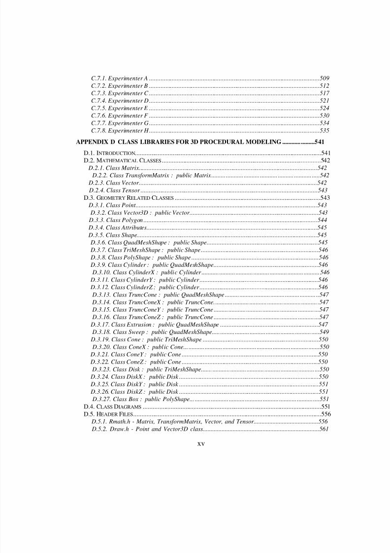
C.7.1. Experimenter A .........................................................................................................509
C.7.2. Experimenter B .........................................................................................................512
C.7.3. Experimenter C .........................................................................................................517
C.7.4. Experimenter D.........................................................................................................521
C.7.5. Experimenter E .........................................................................................................524
C.7.6. Experimenter F .........................................................................................................530
C.7.7. Experimenter G.........................................................................................................534
C.7.8. Experimenter H.........................................................................................................535
APPENDIX D CLASS LIBRARIES FOR 3D PROCEDURAL MODELING .....................541
D.1. INTRODUCTION..................................................................................................................541D.2. MATHEMATICAL CLASSES .................................................................................................542
D.2.1. Class Matrix..............................................................................................................542
D.2.2. Class TransformMatrix : public Matrix......... ........... .......... ........... .......... ........... .....542
D.2.3. Class Vector..............................................................................................................542
D.2.4. Class Tensor .............................................................................................................543
D.3. GEOMETRY RELATED CLASSES .........................................................................................543 D.3.1. Class Point................................................................................................................543
D.3.2. Class Vector3D : public Vector...............................................................................543
D.3.3. Class Polygon ...........................................................................................................544
D.3.4. Class Attributes.........................................................................................................545
D.3.5. Class Shape...............................................................................................................545
D.3.6. Class QuadMeshShape : public Shape....................................................................545
D.3.7. Class TriMeshShape : public Shape........................................................................546
D.3.8. Class PolyShape : public Shape ..............................................................................546
D.3.9. Class Cylinder : public QuadMeshShape................................................................546
D.3.10. Class CylinderX : public Cylinder........... .......... ........... .......... ........... .......... ..........546
D.3.11. Class CylinderY : public Cylinder.........................................................................546
D.3.12. Class CylinderZ : public Cylinder.........................................................................546
D.3.13. Class TruncCone : public QuadMeshShape ......... ......... .......... ......... ......... .......... ..547
D.3.14. Class TruncConeX : public TruncCone............ .......... ........... .......... ........... .......... .547
D.3.15. Class TruncConeY : public TruncCone ......... ........... .......... ........... ........... .......... ...547
D.3.16. Class TruncConeZ : public TruncCone ......... ........... .......... ........... ........... .......... ...547
D.3.17. Class Extrusion : public QuadMeshShape ............................................................547
D.3.18. Class Sweep : public QuadMeshShape..... ......... ......... .......... ......... ......... .......... .....549
D.3.19. Class Cone : public TriMeshShape .......................................................................550
D.3.20. Class ConeX : public Cone............. ........... .......... ........... .......... ........... ........... .......550
D.3.21. Class ConeY : public Cone ....................................................................................550
D.3.22. Class ConeZ : public Cone ....................................................................................550
D.3.23. Class Disk : public TriMeshShape....... ........... .......... ........... .......... ........... .......... ...550
D.3.24. Class DiskX : public Disk ......................................................................................550
D.3.25. Class DiskY : public Disk ......................................................................................551
D.3.26. Class DiskZ : public Disk ......................................................................................551
D.3.27. Class Box : public PolyShape............. ........... .......... ........... .......... ........... .......... ....551
D.4. CLASS DIAGRAMS .............................................................................................................551D.5. HEADER FILES...................................................................................................................556
D.5.1. Rmath.h - Matrix, TransformMatrix, Vector, and Tensor.........................................556
D.5.2. Draw.h - Point and Vector3D class..........................................................................561
8/3/2019 Chetan Kapoor Dissertation
http://slidepdf.com/reader/full/chetan-kapoor-dissertation 16/612
xvi
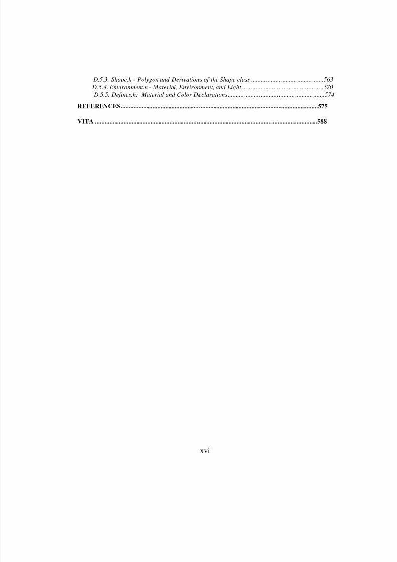
D.5.3. Shape.h - Polygon and Derivations of the Shape class ......... .......... ......... ......... .......563
D.5.4. Environment.h - Material, Environment, and Light .................................................570
D.5.5. Defines.h: Material and Color Declarations.......... .......... ........... .......... ........... .......574
REFERENCES............................................................................................................................575
VITA ............................................................................................................................................588
8/3/2019 Chetan Kapoor Dissertation
http://slidepdf.com/reader/full/chetan-kapoor-dissertation 17/612
xvii
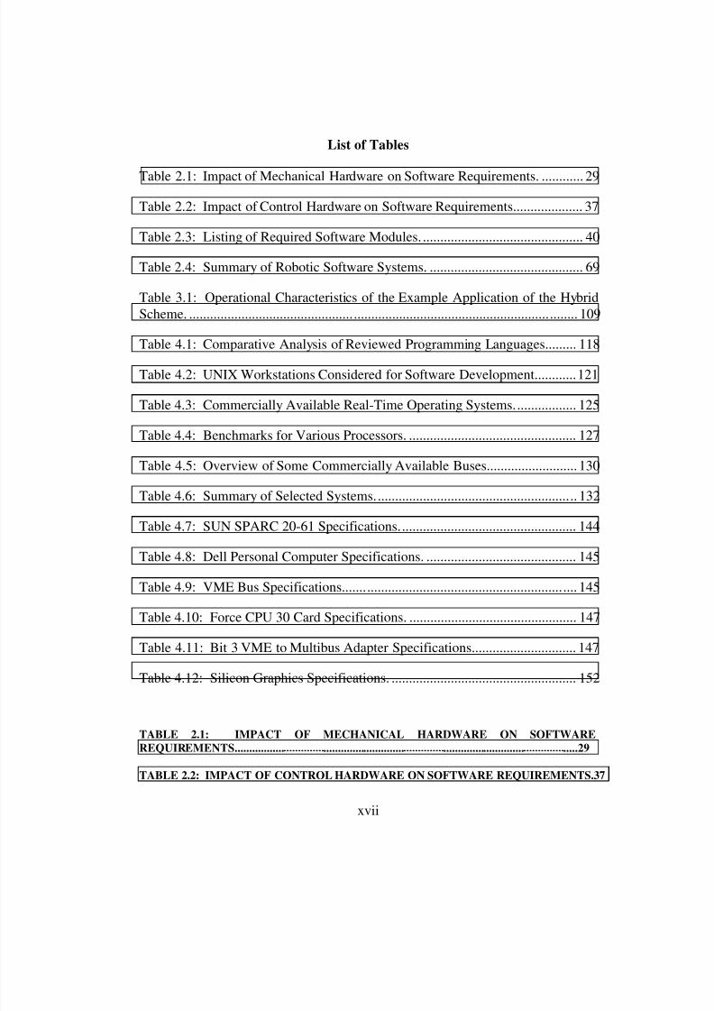
List of Tables
Table 2.1: Impact of Mechanical Hardware on Software Requirements. ............ 29
Table 2.2: Impact of Control Hardware on Software Requirements.................... 37
Table 2.3: Listing of Required Software Modules. .............................................. 40
Table 2.4: Summary of Robotic Software Systems. ............................................ 69
Table 3.1: Operational Characteristics of the Example Application of the Hybrid
Scheme. ............................................................................................................... 109
Table 4.1: Comparative Analysis of Reviewed Programming Languages......... 118
Table 4.2: UNIX Workstations Considered for Software Development............121
Table 4.3: Commercially Available Real-Time Operating Systems.................. 125
Table 4.4: Benchmarks for Various Processors. ................................................ 127
Table 4.5: Overview of Some Commercially Available Buses.......................... 130
Table 4.6: Summary of Selected Systems.......................................................... 132
Table 4.7: SUN SPARC 20-61 Specifications................................................... 144
Table 4.8: Dell Personal Computer Specifications. ........................................... 145
Table 4.9: VME Bus Specifications................................................................... 145
Table 4.10: Force CPU 30 Card Specifications. ................................................ 147
Table 4.11: Bit 3 VME to Multibus Adapter Specifications.............................. 147
Table 4.12: Silicon Graphics Specifications. ..................................................... 152
TABLE 2.1: IMPACT OF MECHANICAL HARDWARE ON SOFTWARE
REQUIREMENTS........................................................................................................................29
TABLE 2.2: IMPACT OF CONTROL HARDWARE ON SOFTWARE REQUIREMENTS.37
8/3/2019 Chetan Kapoor Dissertation
http://slidepdf.com/reader/full/chetan-kapoor-dissertation 18/612
xviii
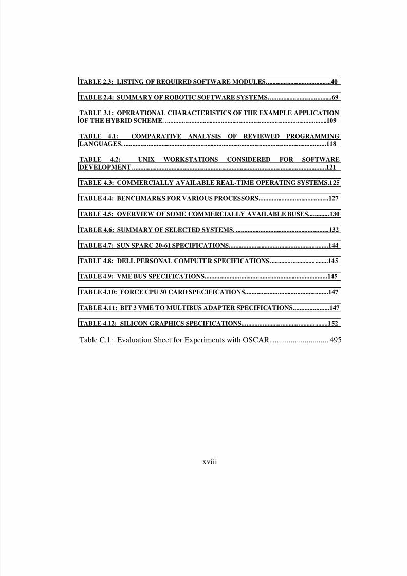
TABLE 2.3: LISTING OF REQUIRED SOFTWARE MODULES........................................40
TABLE 2.4: SUMMARY OF ROBOTIC SOFTWARE SYSTEMS.......................................69
TABLE 3.1: OPERATIONAL CHARACTERISTICS OF THE EXAMPLE APPLICATION
OF THE HYBRID SCHEME. ...................................................................................................109
TABLE 4.1: COMPARATIVE ANALYSIS OF REVIEWED PROGRAMMING
LANGUAGES. ............................................................................................................................118
TABLE 4.2: UNIX WORKSTATIONS CONSIDERED FOR SOFTWARE
DEVELOPMENT. ......................................................................................................................121
TABLE 4.3: COMMERCIALLY AVAILABLE REAL-TIME OPERATING SYSTEMS.125
TABLE 4.4: BENCHMARKS FOR VARIOUS PROCESSORS...........................................127
TABLE 4.5: OVERVIEW OF SOME COMMERCIALLY AVAILABLE BUSES.............130
TABLE 4.6: SUMMARY OF SELECTED SYSTEMS. .........................................................132
TABLE 4.7: SUN SPARC 20-61 SPECIFICATIONS.............................................................144
TABLE 4.8: DELL PERSONAL COMPUTER SPECIFICATIONS....................................145
TABLE 4.9: VME BUS SPECIFICATIONS...........................................................................145
TABLE 4.10: FORCE CPU 30 CARD SPECIFICATIONS...................................................147
TABLE 4.11: BIT 3 VME TO MULTIBUS ADAPTER SPECIFICATIONS......................147
TABLE 4.12: SILICON GRAPHICS SPECIFICATIONS.....................................................152
Table C.1: Evaluation Sheet for Experiments with OSCAR. ............................ 495
8/3/2019 Chetan Kapoor Dissertation
http://slidepdf.com/reader/full/chetan-kapoor-dissertation 19/612
xix
List of Figures
Figure 1.1: The Three Layers of Robotic Software................................................ 4
Figure 2.1: The I-STAR Environment for System Design................................... 19
Figure 2.2: A Six DOF Monolithic Robot. .......................................................... 22
Figure 2.3: A Six DOF Modular Robot. .............................................................. 23
Figure 2.4: Exploded View of the Modular Robot. ............................................. 24
Figure 2.5: A Ten DOF Fault-Tolerant Manipulator. .......................................... 25
Figure 2.6: Centralized Control Structure [Puls, 1994]. ...................................... 31
Figure 2.7: Distributed Control Structure [Puls, 1994]........................................ 32
Figure 2.8: Structured Program Design................................................................ 42
Figure 2.9: Abstract Data Type Matrix. ............................................................... 47
Figure 2.10: Matrix Class Inheritance.................................................................. 48
Figure 2.11: Ad hoc Style of Real-Time Software Design. ................................. 54
Figure 2.12: Task-Based Real-Time Software Design......................................... 56
Figure 2.13: Desired Functionality of the Operational Software Layer. .............. 74
Figure 3.1: A Three DOF Planar Robot. .............................................................. 81
Figure 3.2: A Hypercube Representing the Explorations for a Three DOF Robot[Hooper, 1994]. ..................................................................................................... 86
Figure 3.3: Self-Motion of a Redundant Arm...................................................... 87
Figure 3.4: Inverse Kinematics Using Direct-Search and a Closed-Form InversePosition Solution. .................................................................................................. 88
Figure 3.5: Hybrid Formulation for Generalized Inverse..................................... 91
Figure 3.5: Single Criterion Optimization. .......................................................... 97

8/3/2019 Chetan Kapoor Dissertation
http://slidepdf.com/reader/full/chetan-kapoor-dissertation 20/612
xx
Figure 3.6: An Example of Criteria Fusion.......................................................... 98
Figure 3.7: Ambiguity in Options Selection - Demonstration of Need for CriteriaNormalization........................................................................................................ 99
Figure 3.8: Ambiguity in Options Selection - Need for Variance...................... 100
Figure 3.9: Left Arm During a Section of the Experimental Trajectory............ 103
Figure 3.10: Overall Selected Solution and Best Solution for MOT. ................ 104
Figure 3.11: Overall Selected Solution and Best Solution for JVM. ................. 105
Figure 3.12: Overall Selected Solution and Best Solution for JRA................... 106
Figure 3.13: Variation in Ranking of the Overall Best Solution along the
Trajectory for Individual Criterion...................................................................... 107
Figure 4.1: A Self-Hosted System...................................................................... 113
Figure 4.2: A Cross-development System.......................................................... 114
Figure 4.3: Final Development and Execution Environment............................. 133
Figure 4.4: Multi-user Execution and Test Environment................................... 135
Figure 4.6: Simulation and Physical Robot Support for Testing. ...................... 139
Figure 4.7: Software Development, Execution, and Test Environment............. 142
Figure 4.8: VME Chassis with Plugged in Boards............................................. 146
Figure 4.9: TOS Manual Controller. .................................................................. 148
Figure 4.10: Kraft Manual Controller. ............................................................... 149
Figure 4.11: NASA Perforce Manual Controller. .............................................. 150
Figure 4.12: The TeachBall Input Device. ......................................................... 151
Figure 4.13: The Robotics Research Corporation Dual-Arm Robot.................. 153
Figure 4.14: Future Distributed Environment for Cell Control. ........................ 157

8/3/2019 Chetan Kapoor Dissertation
http://slidepdf.com/reader/full/chetan-kapoor-dissertation 21/612
xxi
FIGURE 1.1: THE THREE LAYERS OF ROBOTIC SOFTWARE........................................4
FIGURE 2.1: THE I-STAR ENVIRONMENT FOR SYSTEM DESIGN...............................19
FIGURE 2.2: A SIX DOF MONOLITHIC ROBOT. ...............................................................22
FIGURE 2.3: A SIX DOF MODULAR ROBOT.......................................................................23
FIGURE 2.4: EXPLODED VIEW OF THE MODULAR ROBOT.........................................24
FIGURE 2.5: A TEN DOF FAULT-TOLERANT MANIPULATOR. ....................................25
FIGURE 2.6: CENTRALIZED CONTROL STRUCTURE [PULS, 1994]. ............................31
FIGURE 2.7: DISTRIBUTED CONTROL STRUCTURE [PULS, 1994]. .............................32
FIGURE 2.8: STRUCTURED PROGRAM DESIGN. .............................................................42
FIGURE 2.9: ABSTRACT DATA TYPE MATRIX.................................................................47
FIGURE 2.10: MATRIX CLASS INHERITANCE..................................................................48
FIGURE 2.11: AD HOC STYLE OF REAL-TIME SOFTWARE DESIGN..........................54
FIGURE 2.12: TASK-BASED REAL-TIME SOFTWARE DESIGN.....................................56
FIGURE 2.13: DESIRED FUNCTIONALITY OF THE OPERATIONAL SOFTWARELAYER...........................................................................................................................................74
FIGURE 3.1: A THREE DOF PLANAR ROBOT....................................................................81
FIGURE 3.2: A HYPERCUBE REPRESENTING THE EXPLORATIONS FOR A THREE
DOF ROBOT [HOOPER, 1994]..................................................................................................86
FIGURE 3.3: SELF-MOTION OF A REDUNDANT ARM. ...................................................87
FIGURE 3.4: INVERSE KINEMATICS USING DIRECT-SEARCH AND A CLOSED-
FORM INVERSE POSITION SOLUTION. ..............................................................................88
FIGURE 3.5: HYBRID FORMULATION FOR GENERALIZED INVERSE. .....................91
FIGURE 3.5: SINGLE CRITERION OPTIMIZATION..........................................................97
FIGURE 3.6: AN EXAMPLE OF CRITERIA FUSION..........................................................98
8/3/2019 Chetan Kapoor Dissertation
http://slidepdf.com/reader/full/chetan-kapoor-dissertation 22/612
xxii
FIGURE 3.7: AMBIGUITY IN OPTIONS SELECTION - DEMONSTRATION OF NEED
FOR CRITERIA NORMALIZATION.......................................................................................99
FIGURE 3.8: AMBIGUITY IN OPTIONS SELECTION - NEED FOR VARIANCE........100
FIGURE 3.9: LEFT ARM DURING A SECTION OF THE EXPERIMENTAL
TRAJECTORY. ..........................................................................................................................103
FIGURE 3.10: OVERALL SELECTED SOLUTION AND BEST SOLUTION FOR MOT.104
FIGURE 3.11: OVERALL SELECTED SOLUTION AND BEST SOLUTION FOR JVM.105
FIGURE 3.12: OVERALL SELECTED SOLUTION AND BEST SOLUTION FOR JRA.106
FIGURE 3.13: VARIATION IN RANKING OF THE OVERALL BEST SOLUTION
ALONG THE TRAJECTORY FOR INDIVIDUAL CRITERION........................................107
FIGURE 4.1: A SELF-HOSTED SYSTEM.............................................................................113
FIGURE 4.2: A CROSS-DEVELOPMENT SYSTEM. ..........................................................114
FIGURE 4.3: FINAL DEVELOPMENT AND EXECUTION ENVIRONMENT. ..............133
FIGURE 4.4: MULTI-USER EXECUTION AND TEST ENVIRONMENT. ......................135
FIGURE 4.6: SIMULATION AND PHYSICAL ROBOT SUPPORT FOR TESTING. .....139
FIGURE 4.7: SOFTWARE DEVELOPMENT, EXECUTION, AND TEST
ENVIRONMENT........................................................................................................................142
FIGURE 4.8: VME CHASSIS WITH PLUGGED IN BOARDS...........................................146
FIGURE 4.9: TOS MANUAL CONTROLLER......................................................................148
FIGURE 4.10: KRAFT MANUAL CONTROLLER..............................................................149
FIGURE 4.11: NASA PERFORCE MANUAL CONTROLLER. .........................................150
FIGURE 4.12: THE TEACHBALL INPUT DEVICE............................................................151
FIGURE 4.13: THE ROBOTICS RESEARCH CORPORATION DUAL-ARM ROBOT.153
FIGURE 4.14: FUTURE DISTRIBUTED ENVIRONMENT FOR CELL CONTROL......157
Figure C.1: Directory Structure for OSCAR Source Code Organization. ......... 491
8/3/2019 Chetan Kapoor Dissertation
http://slidepdf.com/reader/full/chetan-kapoor-dissertation 23/612
xxiii
Figure D.1: Normal Calculation for a Polygon. ................................................. 544
Figure D.2: Coordinate Specification for an I-BEAM Extrusion. ..................... 548
Figure D.3: Class Diagram One. ........................................................................ 552
Figure D.4: Class Diagram Two. ....................................................................... 553
Figure D.5: Class Diagram Three. ..................................................................... 554
Figure D.6: Class Diagram Four. ....................................................................... 555
8/3/2019 Chetan Kapoor Dissertation
http://slidepdf.com/reader/full/chetan-kapoor-dissertation 24/612
xxiv
Nomenclature
ADT Abstract Data TypeANSI American National Standards Institute
ASCII American Standard Code for Information InterchangeASME American Society of Mechanical EngineersCAD Computer Aided Design
CPU Central Processing UnitDH Denavit-HartenbergDOF Degree-of-Freedom
GPIB General Purpose Interface BusGUI Graphical User InterfaceI/O Input/Output
IBM International Business Machines CorporationIEEE Institute of Electrical and Electronic EngineersISO Industry Standards Organization
MAX Maximumms millisecond
OS Operating SystemOSCAR Operational Software Components for Advanced RoboticsPC Personal Computer
PID Proportional, Integral, and DerivativePLC Programmable Logic ControlRAM Random Access Memory
RISC Reduced Instruction Set ComputingRPL Robot Programming LanguageRTOS Real Time Operating System
TCP Transmission Control ProtocolOOA Object-oriented AnalysisOOD Object-oriented Design
OOP Object-oriented ProgrammingSVD Singular Value Decomposition
8/3/2019 Chetan Kapoor Dissertation
http://slidepdf.com/reader/full/chetan-kapoor-dissertation 25/612
1
Chapter One
1. Introduction
Mechanical systems for manufacturing in the past have represented
monolithic dedicated machines that remained expensive and were inflexible to
product changes due to market demands. Industrial robots, which are key players
in the intelligent machines arena, also exhibit a monolithic mechanical structure
and a closed-system software architecture [Tesar, 1989]. Computer systems by
contrast are increasingly modular, easily upgradable, and rapidly reconfigurable to
meet customer requirements. Robotics research today is focusing on developing
systems that exhibit modularity, flexibility, redundancy, fault-tolerance, a general
and extensible software environment, and seamless connectivity to other
machines.
A modularity-based mechanical structure of machines (robots), coupled
with advancements in computer technology now makes a universal control system
software possible for a very large class of machines. This operating system must
be able to support the development of a full manufacturing cell made up of
fixtures, handling systems, assembly devices, forming sub-systems, etc. The
software architecture for these systems must provide for modularity, software
reuse, rapid-prototyping, and should support generalized kinematics, generalized
8/3/2019 Chetan Kapoor Dissertation
http://slidepdf.com/reader/full/chetan-kapoor-dissertation 26/612
2
dynamics, deflection modeling, performance criteria, criteria-fusion, and fault-
tolerance. These are the essential characteristics of an advanced robotics system
and a full implementation of these is necessary to uplift the standard of US
manufacturing, which over the past ten years has seen a $150 billion/year trade
deficit [Tesar, 1994].
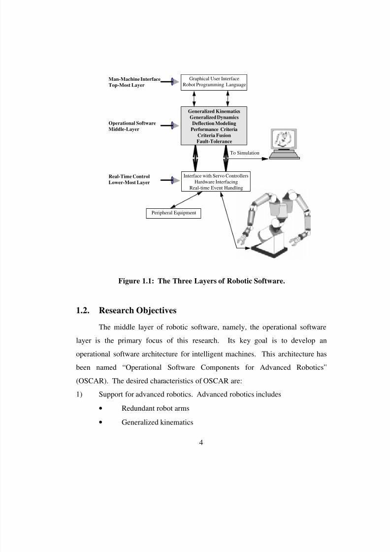
1.1. The Three Layers of a Robotic Software System
A robotic software system at the system controller level can be broadly
divided into three layers. The lower-most layer of this system is the hardware-
interface layer. The purpose of this layer is to interface with the servo control
software, peripheral devices, and communication buses. Real-time constraints on
this layer are the most stringent because it interacts with the external hardware. A
parallel software execution environment is best-suited for this layer. This is
because the software in this layer has to handle multiple asynchronous events
(both external and internal) in real-time (less than 1 millisecond).
The top-most layer of a robotic software system is the robot programming
language. This layer provides the man-machine interface. In this layer, programs
written in the robot programming language (RPL) are converted into appropriate
commands for the middle layer. These commands are then translated into
actuator position, velocity and torque commands by the middle layer which are
then sent to the lowest layer.
The middle-layer of the robotic software system is what is referred to
as the operational software layer. Most industrial robots are six degrees-of-
freedom (DOF) arms and have geometries that allow for simple kinematics and
dynamics. As such, their operational software layer is not very demanding and
offers limited capability. For advanced robots, which exhibit reconfigurability,
redundancy, and fault-tolerance, exceptional demands are placed on the

8/3/2019 Chetan Kapoor Dissertation
http://slidepdf.com/reader/full/chetan-kapoor-dissertation 27/612
3
operational software. It is desired that this layer of software be robot independent,
reconfigurable if there is a fault, and support software reuse and rapid-
prototyping. Also, the operational software architecture should support
generalized kinematics, generalized dynamics, deflection modeling, performance
criteria, and fault-tolerance in a reusable and modular software architecture. As
this layer relies heavily on compute intensive constructs, it should allow for multi-
processor execution and computational efficiency. Additionally, as most concepts
implemented in this layer are under development, the operational software should
be equally applicable to simulation. This feature allows for algorithm testing
before use on physical hardware. The necessity for compatibility with simulation
is even greater as the operational software architecture being proposed in this
research allows for extensibility and user-modification. The user of this
architecture should be able to test any extensions or modifications to the software
before controlling a physical robot. The three layers of robotic software at the
system controller level are illustrated in Figure 1.1.
8/3/2019 Chetan Kapoor Dissertation
http://slidepdf.com/reader/full/chetan-kapoor-dissertation 28/612
4
Graphical User Interface
Robot Programming Language
Generalized Kinematics
Generalized Dynamics
Deflection Modeling
Performance Criteria
Criteria Fusion
Fault-Tolerance
Interface with Servo Controllers
Hardware Interfacing
Real-time Event Handling
Man-Machine Interface
Top-Most Layer
Operational Software
Middle-Layer
Real-Time Control
Lower-Most Layer
Peripheral Equipment
To Simulation
Figure 1.1: The Three Layers of Robotic Software.
1.2. Research Objectives
The middle layer of robotic software, namely, the operational software
layer is the primary focus of this research. Its key goal is to develop an
operational software architecture for intelligent machines. This architecture has
been named “Operational Software Components for Advanced Robotics”
(OSCAR). The desired characteristics of OSCAR are:
1) Support for advanced robotics. Advanced robotics includes
• Redundant robot arms
• Generalized kinematics

8/3/2019 Chetan Kapoor Dissertation
http://slidepdf.com/reader/full/chetan-kapoor-dissertation 29/612
5
• Criteria-based decision making
•
Generalized dynamics• Deflection modeling
• Fault-tolerance
2) Completely general software architecture applicable to any serial arm
3) Applicability to real-time control
4) Applicability to simulation
5) Reuse via extensibility
6) Support rapid-prototyping.
7) Reduced control program development time (50% improvement over
previous robotic software architectures in use at the University of Texas
Robotics Research Group).
Besides the key goal of developing an operational software architecture,
with the above characteristics, the other goals that have to be accomplished as a
part of this research are:
• Selection and development of the software development, execution, and test
environment.
• Training of future users of this software architecture.
• Achievement of a practical implementation of Hooper’s [1994] generalized
inverse kinematics scheme.
The development of such an architecture is a challenging task for two
reasons. The first is the inherent complexity of software. The complexity of
software can be attributed to four factors as specified by Booch [1994]. These
are:
• the complexity of the problem domain,
• the difficulty of managing the developmental process,
• the flexibility possible through software, and
8/3/2019 Chetan Kapoor Dissertation
http://slidepdf.com/reader/full/chetan-kapoor-dissertation 30/612
6
• the problem of characterizing the behavior of discrete systems.
Additionally, software users often underestimate the complexity of software. This is best illustrated by the fact that a builder rarely asks for the
addition of a basement to an 100 story building. On the other hand, users of
software systems rarely think twice about asking for equivalent changes, arguing
that, it is merely a matter of programming [Booch, 1994].
The second reason that makes the development of an operational software
architecture a challenging task is the complexity of the problem domain, that is,
advanced robotics. Developing a reusable architecture for this domain involves
detailed understanding of all advanced robotic concepts: concepts that are further
based on rigorous mathematical formulations. Also, some of the concepts of
advanced robotics are not fully developed. This adds ambiguity to the problem
domain and limits the reuse potential of the software architecture. Additionally,
the translation of a mathematical formulation (which may be expressed as a
simple equation) may take hundred’s of lines of high-level code.
The following sections in this chapter discuss some of the characteristics
of advanced robotics that this research will address. The last section gives an
overview about what follows in this report.
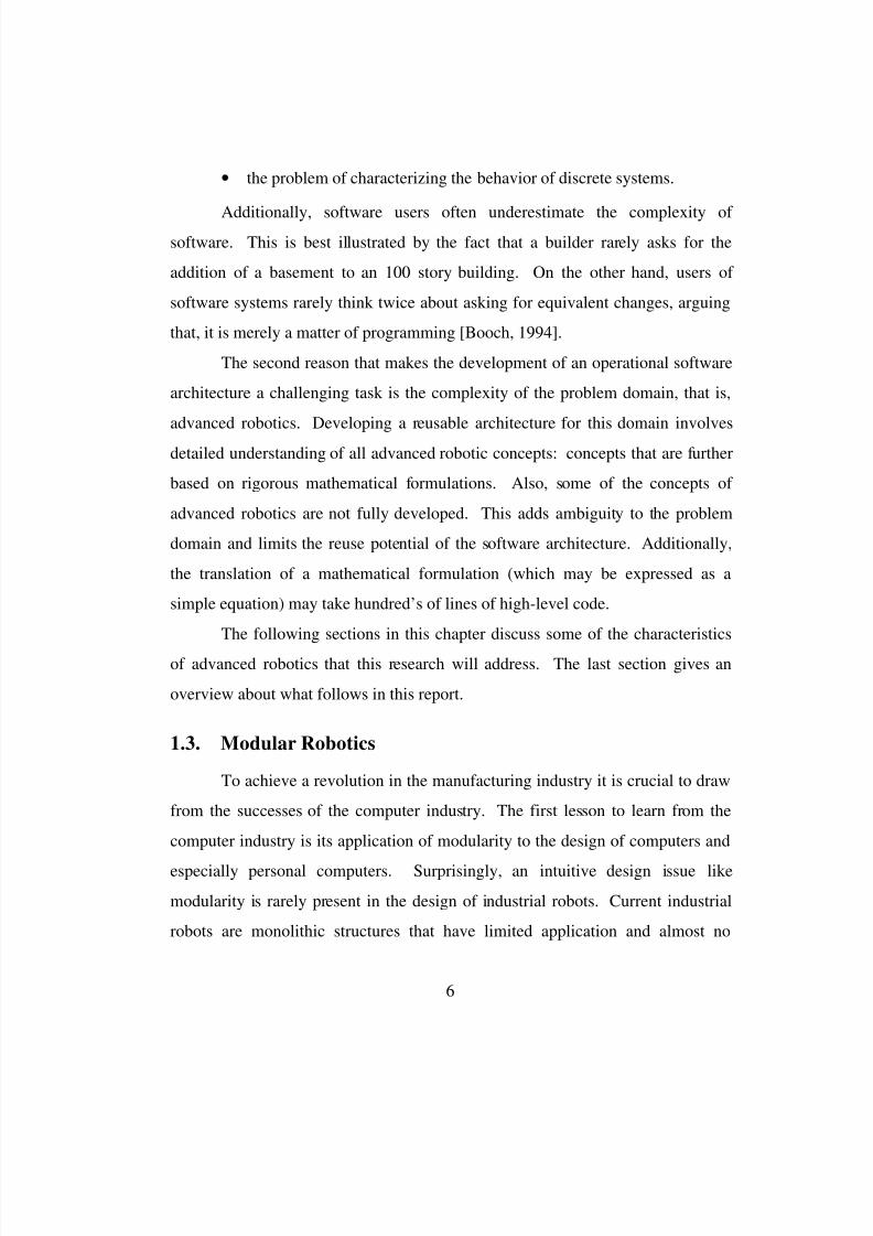
1.3. Modular Robotics
To achieve a revolution in the manufacturing industry it is crucial to draw
from the successes of the computer industry. The first lesson to learn from the
computer industry is its application of modularity to the design of computers and
especially personal computers. Surprisingly, an intuitive design issue like
modularity is rarely present in the design of industrial robots. Current industrial
robots are monolithic structures that have limited application and almost no

8/3/2019 Chetan Kapoor Dissertation
http://slidepdf.com/reader/full/chetan-kapoor-dissertation 31/612
7
upgradability options. On the other hand, a personal computer offers us the best
example of modularity and upgradability. Modularity provides us with a system
that has standardized interfaces and plug-and-play capability. Also, due to the
availability of various modules that maintain standard interfaces, a modular robot
may be configured for a particular task and then quickly reconfigured later if the
task changes. The University of Texas, Robotics Research Group, has been
aggressively pursuing modular robot technology for over two decades [Butler and
Tesar, 1989]. It is the goal of the Robotics Research Group to design a
mechanical architecture that can rapidly evolve in the same fashion as is now
feasible for a personal computer. This effort has centered around the design of a
family of link, joint, and actuator modules. A low-cost prototype modular robot is
currently (July, 1996) under development. This effort is centered on designing
two actuator modules. The larger of the two actuators is used to constitute the
first three joints of the robot and the smaller actuator is used in the wrist of the
robot. Different link geometries can be used to customize this robot for specific
applications [Grupinski, 1996]. In addition, a project to design and build a high
accuracy seven DOF modular robotic system is in its fifth year of development
[Marrs, 1996].
1.4. Robot Control
Once a good mechanical architecture is available for a modular robot, the
next step involves the computer hardware and software concepts for controlling
the robot. Essentially, the control of the robot is at two levels: the servo level and
the system level. The servo level control is used for controlling each individual
actuator and is characterized by a very high update rate (1000 Hertz). In current
industrial robots the servos are located external to the mechanical structure of the
robot arm. This not only leads to a cabling problem, but also destroys the
8/3/2019 Chetan Kapoor Dissertation
http://slidepdf.com/reader/full/chetan-kapoor-dissertation 32/612
8
modularity of the system. To solve this problem, the Robotics Research Group at
the University of Texas has developed Digital Intelligent Servo Controller (DISC)
technology [Aalund et al., 1993]. These DISC’s are resident within the robot
structure and are responsible for the low level control of the robot and can run
closed-loop control in position, velocity, and acceleration mode.
The other layer in robot control is composed of the system level controller
whose main purpose is to calculate and transmit position, velocity, or
acceleration-level commands to the servos [Aalund, 1991]. Also, a control loop
(for example, hybrid force control) can be executed at the system level to achieve
desired performance. Besides running the closed loop control, the system level
controller is responsible for solving the robot kinematics and dynamics,
compensate for deflection, enhance performance, and interface with external
equipment. Furthermore, the system controller performs the task of resource
management, responds to external events in real-time, and performs decision
making.
1.5. Generalized Kinematics
Kinematics for robot structures involves computing the forward position
solution, which essentially computes the hand position and orientation based on a
known joint angle set. Kinematics also includes the inverse position solution,
which is used to compute joint angles based on a given hand position and
orientation. Kinematics is usually performed at the position, velocity, and
acceleration-level [Craig, 1986]. One way of computing the forward position
solution is to formulate homogenous transformation matrices for each joint of a
robot. These matrices can then be multiplied to get a description of the position
and orientation of the end-effector of the robot. The homogenous transformation
8/3/2019 Chetan Kapoor Dissertation
http://slidepdf.com/reader/full/chetan-kapoor-dissertation 33/612
9
matrices for each joint can be formulated using the Denavit-Hartenberg (DH)
parameters [Craig, 1986].
Position and orientation constraints specify the location of the end-effector
relative to the base of the robot. The inverse kinematics problem is to find the set
of joint displacements satisfying these constraints. A six DOF spatial robot
constitutes a fully motion specified system since there are as many DOF as there
are end-effector specifications (three for position and three for orientation).
Closed-form inverse position solutions are possible for six DOF robots [Craig,
1986]. Numerical solutions are used for redundant robots and they offer the
advantages of generality and reconfiguration [Nakamura, 1993]. A robot with
more DOF than constraints constitutes a redundant robot (an example is a seven
DOF spatial arm). These systems have infinite inverse kinematics solutions
because their Jacobian-based inverse is mathematically non-square. Besides
flexibility, redundancy offers the advantage of incorporation of relevant criteria
that can be used to select a solution that maximizes performance. As advanced
robots are characterized by reconfigurability and redundancy, it is imperative that
the software and algorithm for inverse kinematics be robot independent and
should support criteria-based performance maximization.
1.6. Generalized Dynamics
Along with kinematics, the system controller may calculate the joint
torques required to make the robot end-effector follow a desired trajectory. This
is the inverse dynamics problem and it involves calculating the joint torques based
on a given set of joint positions, velocities, and accelerations. These torques can
be used as signals to be added as feed-forward terms in a conventional feedback
control loop to linearize and decouple the system, thereby improving
performance. This scheme is commonly known as computed torque control
8/3/2019 Chetan Kapoor Dissertation
http://slidepdf.com/reader/full/chetan-kapoor-dissertation 34/612
10
[Izaguirre et al., 1992]. Various techniques have been proposed for inverse
dynamics. Of these the most computationally efficient is the Recursive Newton-
Euler [Craig, 1986]. This technique does not provide a description of the system
inertia, and thus cannot be used in mass distribution-based decision making in the
presence of uncertainty. Thomas and Tesar [1982] have proposed a dynamic
modeling technique for serial manipulators that is based on influence coefficients.
Kinematic influence coefficients are based solely on the geometry of the system.
This technique is useful for design as it provides detailed information about the
system behavior and can thus be used for determining load and size of links and
actuators [Thomas and Tesar, 1982]. It also shows all complex terms and can be
used for studying higher-order properties in real-time.
1.7. Deflection Modeling
Another crucial aspect of the system controller, relevant in light machining
operations, is maintaining zero end-effector position and orientation error
[Wander and Tesar, 1992]. This becomes difficult in the presence of end-effector
loads, and joint and link compliance. To counteract this, the load induced
deflection at the end-effector is calculated based on a full compliance model and
the error is then corrected. This involves the knowledge of the robot link and
joint stiffness matrices and accurate geometric dimensions. The work done by
Hudgens [1992] and Knopf [1994] in the area of modular metrology answers
some questions regarding the accurate parameterization of a modular robot. To
calculate the deflection at the end-effector, Fresonke et al. [1988] have proposed a
deflection modeling technique based on kinematic influence coefficients. In this,
the kinematic analysis based on geometric influence coefficients is used to obtain
resultant joint loads. Based on this, the local link deformations are calculated and
the results are combined to get the end-effector deflection [Fresonke et al., 1988].
8/3/2019 Chetan Kapoor Dissertation
http://slidepdf.com/reader/full/chetan-kapoor-dissertation 35/612
11
1.8. Fault-Tolerance
After the development of a modular robot architecture, the next step in
robotic research is the meaningful application of this architecture. Tesar and
Butler [1989] outlined some applications that would benefit from the
development of modular robot technology. Space station operation is one of these
applications that involves high cost, a hazardous environment for humans, and
requires almost zero-fault operation. The Robotics Research Group at the
University of Texas at Austin is actively pursuing the application of modular
robotics technology to space station operations with an emphasis on fault-tolerance. Sreevijayan and Tesar [1993] have defined fault-tolerance in a robotics
context as “the capability of a system to sustain a failure and still continue
operation without significant impact on the manipulator payload or its immediate
environment.” They also conceptualized a four-level subsumptive architecture for
fault-tolerant robotics. The level I of this architecture involves duality at the
prime mover level [Iaconics, 1991]. This means that a joint actuator is composed
of two identical sub-systems, where both of these sub-systems are operational
under normal conditions. If there is a fault, one sub-system can take care of the
operational needs minimizing the effects on the total system performance. The
second level of fault-tolerance provides extra joints per DOF of the robot. An
example of this is redundantly actuated parallel structures [Yi, 1992]. The third
level of fault-tolerance encompasses redundant robot arms (more than six joints
for a spatial case) [Hooper, 1994]. In this case, a failure in a joint can still leave
the system with “full” functionality. The fourth level of fault-tolerance involves
multi-arm systems. This is a direct reflection of the anthropomorphic paradigm
[Sreevijayan and Tesar, 1993].
8/3/2019 Chetan Kapoor Dissertation
http://slidepdf.com/reader/full/chetan-kapoor-dissertation 36/612
12
As defined by Sreevijayan and Tesar [1993], Level III fault-tolerance
entails the presence of redundancy in the number of joints of a robot arm. The
requirement here is that a robot arm should be able to maintain dexterity and full
access to its workspace if there is a joint failure. This is achieved by imparting
the robot with more DOF than would be required (greater than six in the case of a
spatial robot) [Hooper, 1994]. However, the presence of extra DOF leads to a
non-square system that has infinite solutions. Thus, for any given hand position
and orientation, there are an infinite number of joint solutions. One solution can
be picked from this set based on multiple criteria.
1.9. Decision Making
Noteworthy is that the fault-tolerant architecture, as defined by
Sreevijayan and Tesar [1993], relies on redundancy (alternate physical pathways)
at all levels. However, if a robot structure is designed with redundancies, it is
important that all the DOF of the manipulator be utilized during normal operation.
This is necessary to achieve better dexterity, support obstacle avoidance, and to
avoid mathematical singularities. Utilization of all the degrees of a redundant
manipulator involves solving a system with infinite solutions. This is where
decision making becomes important [Sreevijayan and Tesar, 1993]. The decision
making process in the control of redundant manipulators involves using a set of
performance criteria. These performance criteria can be energy minimization,
manipulator precision, load carrying capacity, speed of operation, or other criteria
[Hooper, 1994]. Based on a given set of performance criteria, decisions are made
as to how to achieve the desired performance. For example, for a kinematically
redundant arm, criteria-based inverse kinematics may involve computing a
solution that minimizes joint velocities. Similarly, other criteria can be
8/3/2019 Chetan Kapoor Dissertation
http://slidepdf.com/reader/full/chetan-kapoor-dissertation 37/612
13
formulated based on geometry, inertia, energy, compliance, and dexterity
measures.
Twenty-nine different performance criteria were identified in one Master’s
thesis alone [VanDoren, 1992]. Also, Cleary and Tesar [1990] have proposed a
set of criteria that are based on the physical parameters of the robot and are
independent of the task. This allows for continuous operation without
reconfiguration if there is a task change. In addition, the work by Hooper [1994]
led to the formulation of a generalized criteria-based inverse solution for
redundant arms. Hooper’s scheme uses the direct-search technique, combined
with a set of constraints (specified by the criteria), to compute the best kinematic
configuration for performing constrained end-effector motion [Hooper, 1994].
However, the presence of multiple criteria, combined with sensory input from
various sources, poses a major problem of criteria fusion. Criteria fusion is
currently an active interest of the Robotics Research Group.
Besides criteria-based decision making, there are other issues that have to
be addressed for fault-tolerant operation of a robot arm. These are failure
detection, diagnosis and estimation, failure recovery and reconfiguration, and
failure treatment. These are necessary and required for fault-tolerant operation. It
should be noted that under normal operation of a redundant arm, the non-
determinancies are resolved based on meaningful decision making criteria. Under
failure conditions, the same redundancies are used to counteract the effects of the
failure. For a smooth transition from normal operation to operation in the
presence of a fault, it is important that the fault-detection and the associated
recovery satisfy real-time constraints [Sreevijayan and Tesar, 1993].
8/3/2019 Chetan Kapoor Dissertation
http://slidepdf.com/reader/full/chetan-kapoor-dissertation 38/612
14
1.10. Overview
The previous sections outlined the characteristics of advanced robotic
systems and discussed some of the issues involved in robotic software systems.
The goal of this research is to develop a software architecture that best fulfills the
requirements of an advanced robotic system. Additionally, this architecture
should provide for software reuse, standardized interfaces and allow for rapid-
prototyping. Another goal of this research is to extend the direct-search technique
of generalized kinematics as proposed by Hooper [1994]. This extended
technique should be computationally efficient, general, reconfigurable, andsupport level III fault-tolerance. Based on this summary, the following
paragraphs outline the contents of this dissertation.
Chapter Two is a critical literature review. The literature review describes
robotic software systems, software design techniques, state of computer
technology, and generalized inverse kinematics. Considering this literature
review, a set of requirements for a software architecture for advanced robots is
derived. Also, an analysis of Hooper’s [1994] work in particular, and inverse
kinematics in general, provides the motivation for further developing Hooper’s
[1994] direct-search technique.
Chapter Three begins by discussing the generalized inverse problem and
then details Hooper’s direct-search technique of inverse kinematics. Based on
this discussion, the strengths and weaknesses of this technique are discussed.
This chapter then details the algorithm for using a combination of the direct-
search technique and a computationally efficient generalized inverse kinematics
scheme. This formulation is called the hybrid formulation. By using a hybrid
formulation, the advantages of the direct-search technique and computationally
efficient generalized scheme can be combined to achieve a practical
8/3/2019 Chetan Kapoor Dissertation
http://slidepdf.com/reader/full/chetan-kapoor-dissertation 39/612
15
implementation. Further, this chapter explains the incorporation of multiple
performance criteria into the hybrid scheme. In addition, a preliminary technique
for criteria fusion is also discussed.
Chapter Four discusses the issues involved in the selection of the hardware
and software environment that was used to develop, demonstrate, and test the
software architecture in question. This involved the selection of a software design
methodology, programming language, operating system, hardware platform,
simulation environment, and robotics hardware. In addition, this chapter discuses
the managerial and organizational issues that were faced in the software
development process.
Chapter Five discusses the core of this research, which involves the design
and development of a software architecture that can best satisfy the needs of
advanced robotic systems. An in-depth analysis of the domain of advanced
robotics is presented. Considering this analysis, the domain of advanced robotics
is broken down into sub-domains. These sub-domains include mathematical
abstractions, forward kinematics, inverse kinematics, dynamics, deflection
modeling, performance criteria, and utility components. These domains are
further broken down into operational software components that have standardized
interfaces and support reuse via generality and extensibility. Details of the
analysis and design issues are provided for each component. Furthermore,
example use and the reuse potential of each operational software component is
discussed.
Chapter Six provides validation for this research. This includes
demonstrations of the software architecture. Various example programs are
shown which depict the simulation and operational characteristics of this
software. Example demonstrations for the generalized inverse and the hybrid
formulation are also shown. Additionally, example programs are given which
8/3/2019 Chetan Kapoor Dissertation
http://slidepdf.com/reader/full/chetan-kapoor-dissertation 40/612
16
depict the extensibility and generality of the software architecture. This chapter
also discusses the experiments conducted with this software architecture. These
experiments were conducted to analyze the benefits of this software architecture
over existing implementations. The criteria used to make this analysis and the
results are discussed here.
Chapter Seven concludes this dissertation and discusses areas for future
work. This chapter discusses the lessons learnt and explains and draws
conclusions from the experimental activity that was performed as a part of this
research. The various issues faced during the analysis and design of the software
architecture are discussed. Additionally, issues relating to implementation,
integration, system control, and manufacturing cells are discussed. Also, other
areas in intelligent machine software that can benefit from a software architecture
are discussed.
8/3/2019 Chetan Kapoor Dissertation
http://slidepdf.com/reader/full/chetan-kapoor-dissertation 41/612
17
Chapter Two
2. Literature Review
2.1. Introduction
Robots are advanced machines that incorporate technology from all
engineering disciplines. This includes mechanical hardware, computer hardware,
and computer software. It is the goal of the Robotics Research Group at the
University of Texas at Austin to design the next generation robot [Tesar, 1989]: a
robot that is based on the concepts of modularity, reconfigurability, fault-tolerance, and enhanced flexibility and performance. For this to be possible, it is
imperative to use the very best in mechanical and computer technology.
The Robotics Research Group is actively pursuing the development of
intelligent machine component technology in all three engineering disciplines
(mechanical hardware, computer hardware, and software). These components
comprise a complete set of modules that would allow building of complete
systems. For this kind of component technology to be successful, a computer
aided design (CAD) system is needed that would allow the selection of the
optimal modules. Work done in this area has led to the development of a CAD
selection process for the mechanical modules (MCAD) [Bunker, 1996], and a
8/3/2019 Chetan Kapoor Dissertation
http://slidepdf.com/reader/full/chetan-kapoor-dissertation 42/612
18
similar CAD procedure for the electrical hardware components (CCAD)
[Ambrose, 1992]. MCAD is responsible for determining the optimum
configuration of the manipulator based on specifications and the available
mechanical modules [Bunker, 1996]. CCAD creates the optimal controller based
on available components [Ambrose, 1992]. The third sub-system of this CAD
tool is SCAD. SCAD stands for software CAD and is the tool that can optimally
select software modules for the task at hand. However, before SCAD can be
fully developed, an architecture for the software components needs to be
developed. The exact requirements of these components, their functionality,
and their interface needs to be defined. The requirements generation and
development of this software architecture is the prime goal of this research.
The software modules developed as a part of this research will span the full
spectrum of operational requirements for advanced robotics, including criteria-
based decision making, generalized inverse kinematics, dynamics, deflection
modeling, etc. These modules will be standardized to fit within a complete
architecture for the advanced robot software system and will be packaged in the
SCAD environment for interactive prioritization, selection, and integration into
the full operating system. The requirement that these modules be efficient,
portable, reliable, maintainable, and operate in real-time, is essential to the
effectiveness of the SCAD process.
Once MCAD, CCAD, and SCAD are fully developed, the next step is the
development of a system that ties all these three sub-systems together and
provides an interface to the user. This requirement has led to the preliminary
development of an Interactive Synthesis Tool for Advanced Robotics (I-STAR)
that deals with the CAD selection process. The I-STAR design environment
allows the user to interactively design a modular robotic manipulator from an
optimum population of hardware and software modules that can best meet the
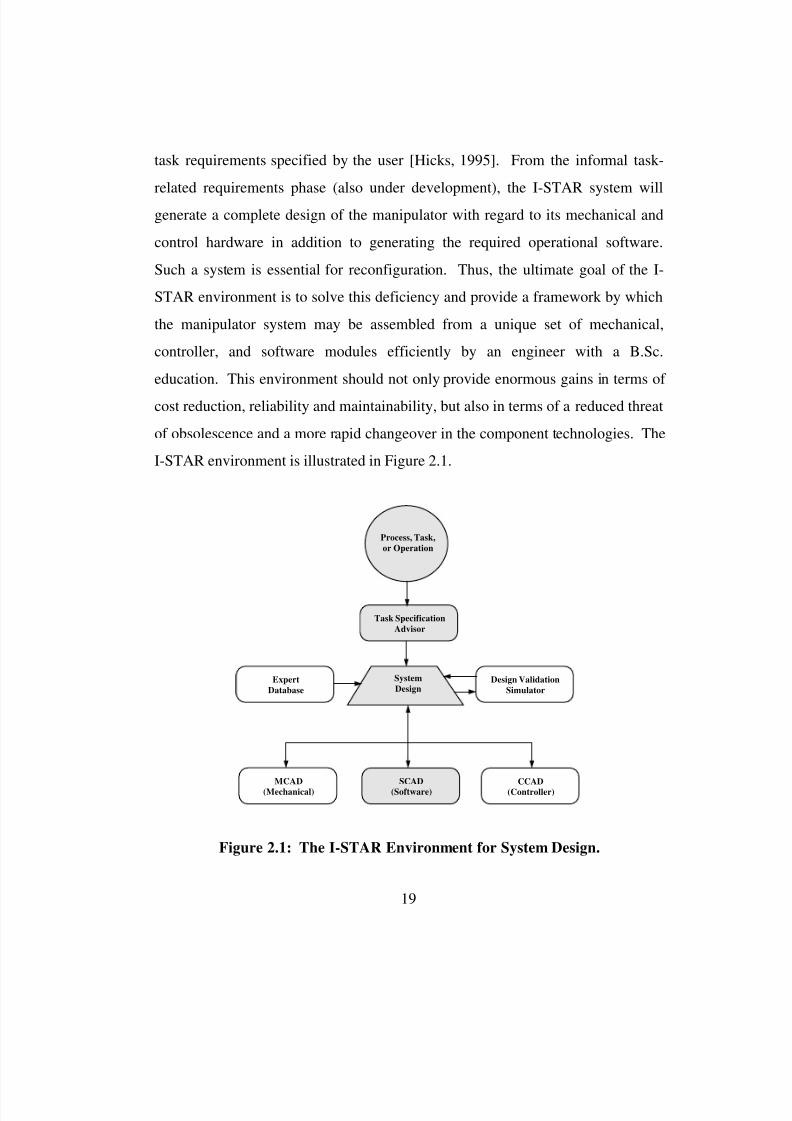
8/3/2019 Chetan Kapoor Dissertation
http://slidepdf.com/reader/full/chetan-kapoor-dissertation 43/612
19
task requirements specified by the user [Hicks, 1995]. From the informal task-
related requirements phase (also under development), the I-STAR system will
generate a complete design of the manipulator with regard to its mechanical and
control hardware in addition to generating the required operational software.
Such a system is essential for reconfiguration. Thus, the ultimate goal of the I-
STAR environment is to solve this deficiency and provide a framework by which
the manipulator system may be assembled from a unique set of mechanical,
controller, and software modules efficiently by an engineer with a B.Sc.
education. This environment should not only provide enormous gains in terms of
cost reduction, reliability and maintainability, but also in terms of a reduced threat
of obsolescence and a more rapid changeover in the component technologies. The
I-STAR environment is illustrated in Figure 2.1.
MCAD(Mechanical) SCAD(Software) CCAD(Controller)
Expert
Database
Design Validation
Simulator
System
Design
Task Specification
Advisor
Process, Task,
or Operation
Figure 2.1: The I-STAR Environment for System Design.
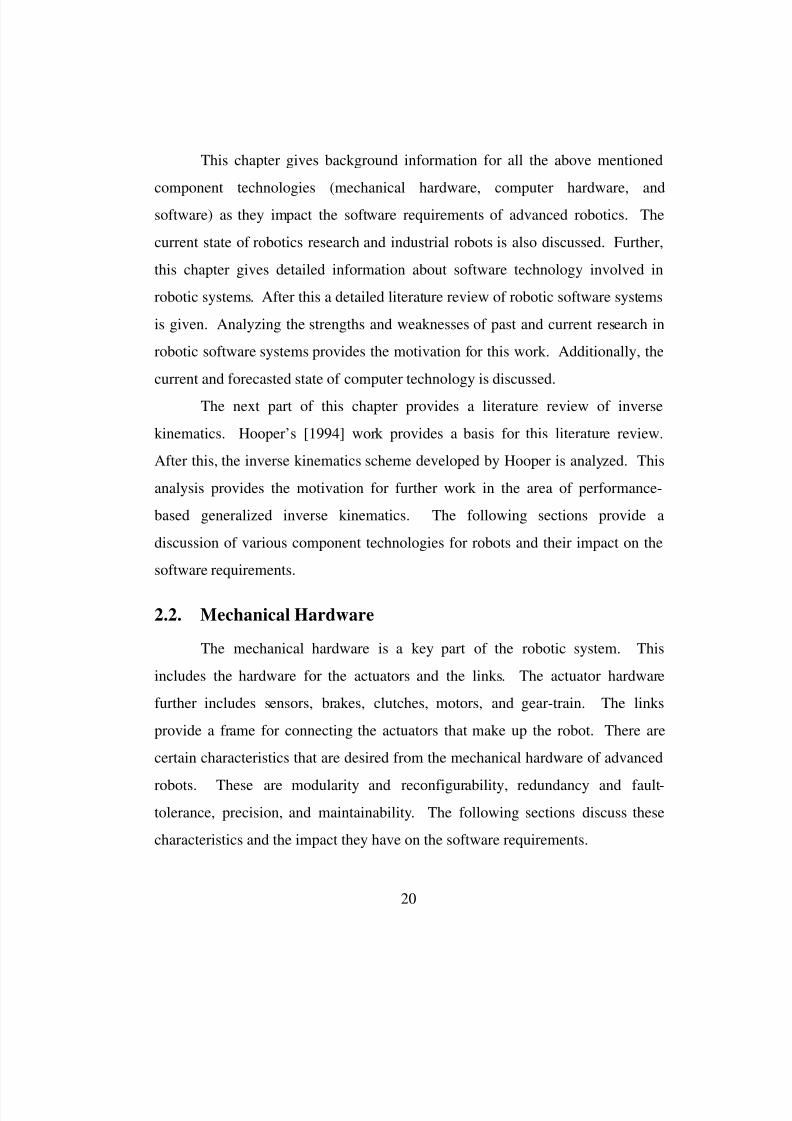
8/3/2019 Chetan Kapoor Dissertation
http://slidepdf.com/reader/full/chetan-kapoor-dissertation 44/612
20
This chapter gives background information for all the above mentioned
component technologies (mechanical hardware, computer hardware, and
software) as they impact the software requirements of advanced robotics. The
current state of robotics research and industrial robots is also discussed. Further,
this chapter gives detailed information about software technology involved in
robotic systems. After this a detailed literature review of robotic software systems
is given. Analyzing the strengths and weaknesses of past and current research in
robotic software systems provides the motivation for this work. Additionally, the
current and forecasted state of computer technology is discussed.
The next part of this chapter provides a literature review of inverse
kinematics. Hooper’s [1994] work provides a basis for this literature review.
After this, the inverse kinematics scheme developed by Hooper is analyzed. This
analysis provides the motivation for further work in the area of performance-
based generalized inverse kinematics. The following sections provide a
discussion of various component technologies for robots and their impact on the
software requirements.
2.2. Mechanical Hardware
The mechanical hardware is a key part of the robotic system. This
includes the hardware for the actuators and the links. The actuator hardware
further includes sensors, brakes, clutches, motors, and gear-train. The links
provide a frame for connecting the actuators that make up the robot. There are
certain characteristics that are desired from the mechanical hardware of advanced
robots. These are modularity and reconfigurability, redundancy and fault-
tolerance, precision, and maintainability. The following sections discuss these
characteristics and the impact they have on the software requirements.
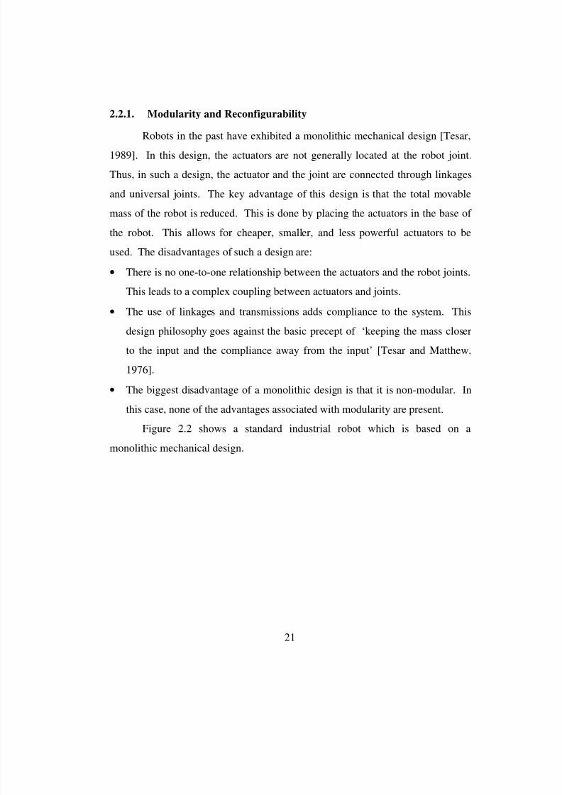
8/3/2019 Chetan Kapoor Dissertation
http://slidepdf.com/reader/full/chetan-kapoor-dissertation 45/612
21
2.2.1. Modularity and Reconfigurability
Robots in the past have exhibited a monolithic mechanical design [Tesar,1989]. In this design, the actuators are not generally located at the robot joint.
Thus, in such a design, the actuator and the joint are connected through linkages
and universal joints. The key advantage of this design is that the total movable
mass of the robot is reduced. This is done by placing the actuators in the base of
the robot. This allows for cheaper, smaller, and less powerful actuators to be
used. The disadvantages of such a design are:
• There is no one-to-one relationship between the actuators and the robot joints.
This leads to a complex coupling between actuators and joints.
• The use of linkages and transmissions adds compliance to the system. This
design philosophy goes against the basic precept of ‘keeping the mass closer
to the input and the compliance away from the input’ [Tesar and Matthew,
1976].
• The biggest disadvantage of a monolithic design is that it is non-modular. In
this case, none of the advantages associated with modularity are present.
Figure 2.2 shows a standard industrial robot which is based on a
monolithic mechanical design.

8/3/2019 Chetan Kapoor Dissertation
http://slidepdf.com/reader/full/chetan-kapoor-dissertation 46/612
22
Actuators for the Wrist
Actuator for the Elbow
Transmission
Shafts add
Compliance
Figure 2.2: A Six DOF Monolithic Robot.
Current trends in robotics research are to design modular robots which are
based on advanced actuator technology [Butler and Tesar, 1989]. Actuators being
developed in the research community now incorporate the motor, sensors, gear-
train, power electronics, servo-controller, and software in one self contained unit.
Such actuators can be placed directly at the robot joint. Using these actuators, a
modular robot can easily be configured as a set of actuators and links connecting
these actuators. Robots which incorporate modularity offer the advantages of
reconfigurability, extensibility, standardization, simplified mechanical
architecture, and enhanced stiffness [Butler and Tesar, 1989]. Figure 2.3 depicts asix DOF modular robot.
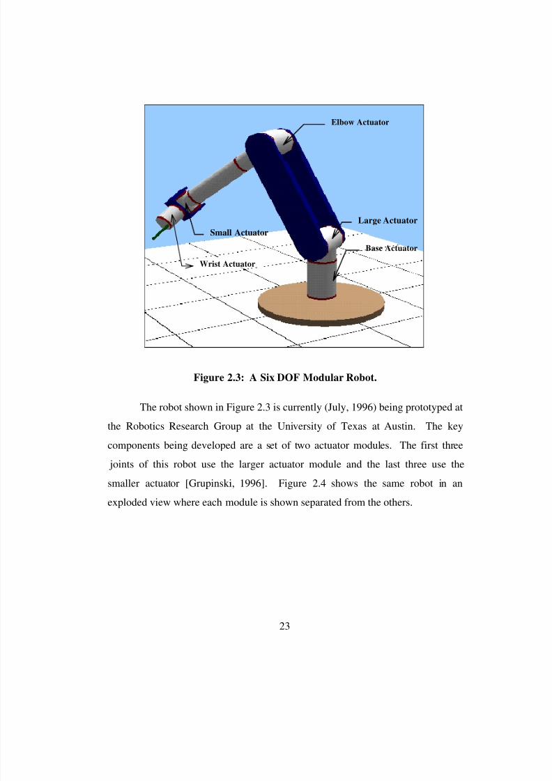
8/3/2019 Chetan Kapoor Dissertation
http://slidepdf.com/reader/full/chetan-kapoor-dissertation 47/612
23
Base Actuator
Wrist Actuator
Large Actuator
Small Actuator
Elbow Actuator
Figure 2.3: A Six DOF Modular Robot.
The robot shown in Figure 2.3 is currently (July, 1996) being prototyped atthe Robotics Research Group at the University of Texas at Austin. The key
components being developed are a set of two actuator modules. The first three
joints of this robot use the larger actuator module and the last three use the
smaller actuator [Grupinski, 1996]. Figure 2.4 shows the same robot in an
exploded view where each module is shown separated from the others.
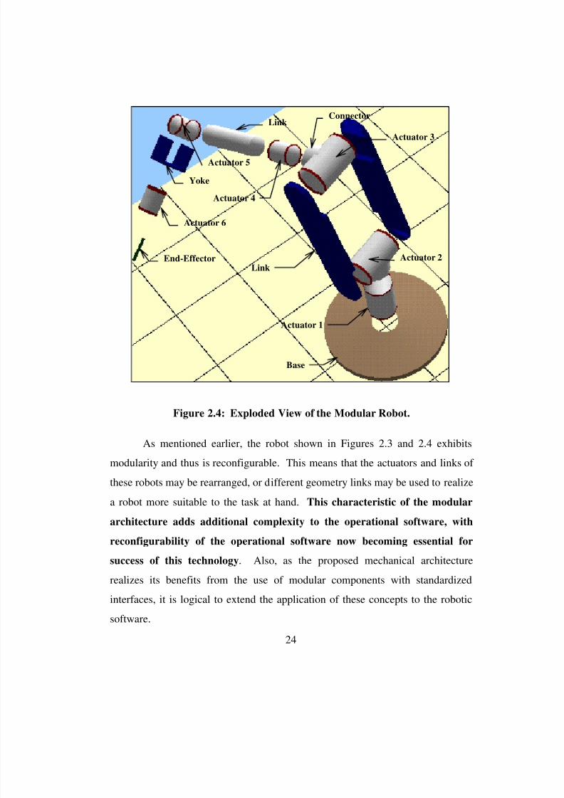
8/3/2019 Chetan Kapoor Dissertation
http://slidepdf.com/reader/full/chetan-kapoor-dissertation 48/612
24
Base
Actuator 1
Actuator 2Link
Actuator 3
Actuator 4
Link
Actuator 5
Actuator 6
Yoke
End-Effector
Connector
Figure 2.4: Exploded View of the Modular Robot.
As mentioned earlier, the robot shown in Figures 2.3 and 2.4 exhibits
modularity and thus is reconfigurable. This means that the actuators and links of
these robots may be rearranged, or different geometry links may be used to realize
a robot more suitable to the task at hand. This characteristic of the modular
architecture adds additional complexity to the operational software, with
reconfigurability of the operational software now becoming essential for
success of this technology. Also, as the proposed mechanical architecture
realizes its benefits from the use of modular components with standardized
interfaces, it is logical to extend the application of these concepts to the robotic
software.

8/3/2019 Chetan Kapoor Dissertation
http://slidepdf.com/reader/full/chetan-kapoor-dissertation 49/612
25
2.2.2. Redundancy and Fault-Tolerance
Once a modular and reconfigurable mechanical architecture is in place, thenext step is to develop advanced robotic devices that exhibit redundancy and
fault-tolerance. Redundancy entails the use of more DOF than the bare minimum
required for the task. Redundancy has the advantages of flexibility, increased
performance, and fault-tolerance. An example of a redundant robot arm is shown
in Figure 2.5. This robot has ten DOF and has a fault-tolerant mechanical
architecture.
Figure 2.5: A Ten DOF Fault-Tolerant Manipulator.
The presence of redundancy and fault-tolerance adds a great deal of
complexity to the robotic software. The biggest reason for this complexity is the
8/3/2019 Chetan Kapoor Dissertation
http://slidepdf.com/reader/full/chetan-kapoor-dissertation 50/612
26
complete change of the domain the software is dealing with. This is because most
of the algorithms and control schemes that apply to non-redundant robot arms are
no longer valid for redundant arms. Also, greater performance is desired from a
redundant mechanical structure. It is the software that has to extract this
performance. The software now has to support generalized kinematics, dynamics,
performance criteria, decision making, and criteria fusion (see Chapter One for a
description of these constructs).
A four-level fault-tolerant mechanical architecture has been defined by
Sreevijayan and Tesar [1993]. This architecture is subsumptive in a sense that the
effects of a fault are not transferred to other layers. The support for fault-
tolerance in the mechanical architecture adds stringent real-time constraints to the
software. Software sub-systems now have to be developed for fault-detection and
identification, fault-tree analysis, and real-time resource allocation [Sreevijayan
and Tesar, 1993]. Additionally, the software itself has to support fault-tolerance.
This is necessary because a fault-tolerant system is only possible if all its sub-
systems exhibit fault-tolerance. As a part of the fault detection and identification
sub-system, software has to be developed for accurate modeling of the robot being
controlled. By comparing the results of the robot modeling software with input
sensor data, aberrations in the robot behavior can be detected. This assists in fault
detection and isolation.
2.2.3. Precision
A majority of current industrial robots are used for simple tasks (pick and
place) that involve little precision work [Tesar, 1989]. As mentioned earlier,advanced robots are being developed that are based on modularity, performance
and fault-tolerance. The full potential of these robots can only be realized if they
are used for “real” manufacturing applications, that is, high-speed and precision
8/3/2019 Chetan Kapoor Dissertation
http://slidepdf.com/reader/full/chetan-kapoor-dissertation 51/612
27
applications that are currently being handled by fixed-automation machines.
Currently the Robotics Research Group is developing a prototype high precision
seven DOF manipulator [Marrs, 1996]. This robot is characterized by a
mechanical structure with minimal compliance and backlash (average deflection
of 0.01 inches and one arc-second of lost-motion) [Marrs, 1996]. Again, the
software will be key to exploiting the functionality of this robot. Under operation,
there will be force-related disturbances created due to the manufacturing process.
Also, the robot end-effector will not be able to maintain desired absolute location
due to compliance in its links and joints under loads. To counteract these
problems it is necessary that the control software compensate for mechanical
deflection and reject disturbance effects.
2.2.4. Maintainability
The development of an advanced mechanical architecture, as the one
proposed in the previous sections, is a costly endeavor. The reliability of these
systems will have to be guaranteed for their effective utilization. Additionally,
down-time, if any, should be minimum for these machines. For this to be
possible, the failures of these machines should be predictable. To achieve this
level of maintainability, unprecedented demands will be placed on the software of
these machines. These machines will be data-base driven. Under operation, the
performance of these machines will be continuously monitored and the empirical
data collected and archived in real-time. This data will then be used for
condition-based maintenance. Continuous comparison of a parameteric model of
the machine to the actual machine condition derived from on-board sensors willalso provide a time-sheet for maintenance. Similar technology is already being
made available in today’s automobiles. Electronics, software, and transducers are
effectively being used in today’s cars to detect and inform the user of the

8/3/2019 Chetan Kapoor Dissertation
http://slidepdf.com/reader/full/chetan-kapoor-dissertation 52/612
28
impending maintenance. It is desired that a similar infusion of technology take
place in the intelligent machines arena.
The previous paragraphs discussed the advanced mechanical architecture
of intelligent machines. This architecture is based on modularity,
reconfigurability, fault-tolerance, precision, and maintainability. The
requirements placed on the software due to these characteristics was also
discussed. Table 2.1 summarizes the attributes of a mechanically advanced robot
and shows their impact on the requirements of the software for these robots.
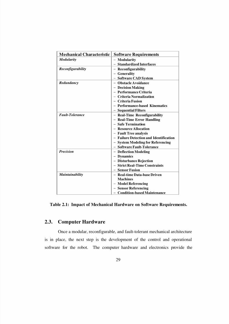
8/3/2019 Chetan Kapoor Dissertation
http://slidepdf.com/reader/full/chetan-kapoor-dissertation 53/612
29
2.3. Computer Hardware
Once a modular, reconfigurable, and fault-tolerant mechanical architecture
is in place, the next step is the development of the control and operational
software for the robot. The computer hardware and electronics provide the
Mechanical Characteristic Software Requirements Modularity − Modularity
− Standardized Interfaces
Reconfigurability − Reconfigurability
− Generality
− Software CAD System
Redundancy − Obstacle Avoidance
− Decision Making
− Performance Criteria
− Criteria Normalization
− Criteria Fusion
− Performance-based Kinematics
− Sequential Filters
Fault-Tolerance − Real-Time Reconfigurability
− Real-Time Error Handling
− Safe Termination
− Resource Allocation
− Fault Tree analysis
− Failure Detection and Identification
− System Modeling for Referencing
− Software Fault-Tolerance
Precision − Deflection Modeling
− Dynamics
− Disturbance Rejection
− Strict Real-Time Constraints
− Sensor Fusion Maintainability − Real-time Data-base Driven
Machines
− Model Referencing
− Sensor Referencing
− Condition-based Maintenance
Table 2.1: Impact of Mechanical Hardware on Software Requirements.

8/3/2019 Chetan Kapoor Dissertation
http://slidepdf.com/reader/full/chetan-kapoor-dissertation 54/612
30
software execution, control and interfacing environment. Section 1.4 had outlined
two major layers of robot control. These were the servo level and system level
control. Both these layers have different software requirements and real-time
constraints. The servo level layer is responsible for the real-time control of the
actuators and has stringent temporal constraints. The system controller is
responsible for operational software and robot programming. The two hardware
layers and their impact on the software requirements is discussed in the following
sections.
2.3.1. Servo-Level Hardware
As stated earlier, the two major software sub-systems have different
software requirements. This difference is also reflected in the computer hardware
and electronics used for the two layers of robot control. At the servo level, power
amplifiers are used to supply current to the actuators. The current is regulated
based on the desired torque output of the actuator. A PID (proportional, integral
and derivative) control loop is generally used to control the position, velocity, and
acceleration of the actuator.
This research is focusing on developing a reusable operational software
architecture. A similar effort is needed in the area of actuator control software.
This software will execute on the servo-level hardware and will have stringent
real-time constraints. Section 7.4.3.1 discusses the issues involved in actuator
control and suggests a preliminary software architecture.
Two approaches are possible for servo-level hardware design. These are
based on centralized control and distributed control. These are discussed in thefollowing sections.
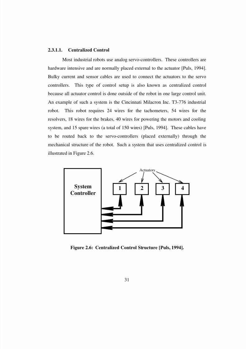
8/3/2019 Chetan Kapoor Dissertation
http://slidepdf.com/reader/full/chetan-kapoor-dissertation 55/612
31
2.3.1.1. Centralized Control
Most industrial robots use analog servo-controllers. These controllers arehardware intensive and are normally placed external to the actuator [Puls, 1994].
Bulky current and sensor cables are used to connect the actuators to the servo
controllers. This type of control setup is also known as centralized control
because all actuator control is done outside of the robot in one large control unit.
An example of such a system is the Cincinnati Milacron Inc. T3-776 industrial
robot. This robot requires 24 wires for the tachometers, 54 wires for the
resolvers, 18 wires for the brakes, 40 wires for powering the motors and cooling
system, and 15 spare wires (a total of 150 wires) [Puls, 1994]. These cables have
to be routed back to the servo-controllers (placed externally) through the
mechanical structure of the robot. Such a system that uses centralized control is
illustrated in Figure 2.6.
System
Controller1 32 4
Actuators
Figure 2.6: Centralized Control Structure [Puls, 1994].

8/3/2019 Chetan Kapoor Dissertation
http://slidepdf.com/reader/full/chetan-kapoor-dissertation 56/612
32
2.3.1.2. Distributed Control
The current trend in robotics research is to develop digital servocontrollers that can be placed inside the actuators. This entails the use of digital
power electronics and an embedded computer which is used to execute the servo-
loop to control the output of the actuator. This technology greatly reduces the
cabling involved in a robotic system and makes the actuator a completely self-
contained unit. Quoting Puls [1994], “depending on the types of power and
communication buses this total number of wires could be less than ten.” This is a
fifteen times reduction over the number of cables used in the T3-776 robot. An
example of the distributed control technology is the Digital Intelligent Servo
Controller (DISC) [Aalund et al., 1993] which accepts position, velocity, or
torque set-points from the system controller. A total of eleven wires is used to
connect a DISC to the system controller and the power supply [Puls, 1994]. A
distributed control structure is illustrated in Figure 2.7.
The previous paragraphs discussed the transition of servo-control
technology from centralized control to distributed control. As a part of this
System
Controller 1 32 4
Actuators
Communicationand Power Bus Local Controllers
Figure 2.7: Distributed Control Structure [Puls, 1994].
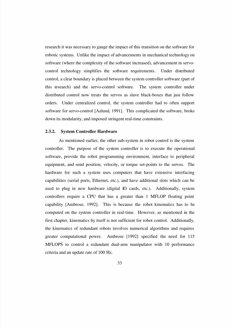
8/3/2019 Chetan Kapoor Dissertation
http://slidepdf.com/reader/full/chetan-kapoor-dissertation 57/612
33
research it was necessary to gauge the impact of this transition on the software for
robotic systems. Unlike the impact of advancements in mechanical technology on
software (where the complexity of the software increased), advancement in servo-
control technology simplifies the software requirements. Under distributed
control, a clear boundary is placed between the system controller software (part of
this research) and the servo-control software. The system controller under
distributed control now treats the servos as slave black-boxes that just follow
orders. Under centralized control, the system controller had to often support
software for servo-control [Aalund, 1991]. This complicated the software, broke
down its modularity, and imposed stringent real-time constraints.
2.3.2. System Controller Hardware
As mentioned earlier, the other sub-system in robot control is the system
controller. The purpose of the system controller is to execute the operational
software, provide the robot programming environment, interface to peripheral
equipment, and send position, velocity, or torque set-points to the servos. The
hardware for such a system uses computers that have extensive interfacing
capabilities (serial ports, Ethernet, etc.), and have additional slots which can be
used to plug in new hardware (digital IO cards, etc.). Additionally, system
controllers require a CPU that has a greater than 1 MFLOP floating point
capability [Ambrose, 1992]. This is because the robot kinematics has to be
computed on the system controller in real-time. However, as mentioned in the
first chapter, kinematics by itself is not sufficient for robot control. Additionally,
the kinematics of redundant robots involves numerical algorithms and requiresgreater computational power. Ambrose [1992] specified the need for 115
MFLOPS to control a redundant dual-arm manipulator with 10 performance
criteria and an update rate of 100 Hz.

8/3/2019 Chetan Kapoor Dissertation
http://slidepdf.com/reader/full/chetan-kapoor-dissertation 58/612
34
Robotics research in the development of system controllers has taken four
different approaches to tackling the hardware requirements. The first approach is
to use rack mounted computers which have many available slots (around ten,
Aalund [1991]) that can be used to connect peripheral equipment. This approach
relies on off-the-shelf hardware. An example of this approach is the multi-
channel robotic controller developed by Aalund [1991].
The second approach to system controller development involves the use of
specialized hardware for compute intensive tasks. This becomes necessary when
the standard computer hardware cannot satisfy the computational needs of the
robot being controlled. An example of this approach is the use of a pipelined
array processor to compute the dynamic model of a robot arm [Wander, 1987].
Using this system Wander was able to compute the complete dynamic model of a
six DOF industrial robot in less than 5 milliseconds.
The third approach to system controller development involves developing
specific computer architectures and hardware for robotics [Ambrose, 1992]. This
was necessary as generic computer hardware was only able (because of its speed
limitations) to compute closed-form inverse kinematics. For example, an Intel
80386-based personal computer (a two MFLOP processor) took more than 100
milliseconds to compute the complete dynamic model of a six DOF robot
[Ambrose, 1992]. Also, various computationally complex mathematical
formulations (dynamics, generalized inverse) required greater than 10 MFLOPS
each and were thus not possible on general purpose hardware.
The fourth approach, which is rapidly gaining popularity, relies on using
standard commercial computer hardware (for example a personal computer) as the
system controller. This has been possible due the increasing computational power
and decreasing cost of commercial computers. Currently (May, 1996), desk-side
uniprocessor computers offer 400 MFLOP performance (R10000 RISC

8/3/2019 Chetan Kapoor Dissertation
http://slidepdf.com/reader/full/chetan-kapoor-dissertation 59/612
35
Microprocessor from MIPS) (refer to Section 2.7 for details on past and current
computer technology). Another advantage of this approach, besides cost and
user-preference, is the availability of software development tools that allow for
easier and state-of-the-art program development (see Chapter Four for details on
software development tools and their selection process). Examples of commercial
system controllers that use personal computers are the system controller from
Cimetrix Incorporated [1996]. This controller uses a Intel Pentium 90 MHz.
CPU as the processor and Windows NT as the operating system and has a total of
thirteen bus slots (ten ISA bus, two PCI bus, and one ISA/PCI).
2.3.3. Computer Bus
Another crucial factor in the development of robotic computer hardware is
the selection of the computer bus, which provides the high-speed communication
link between the system controller and the servo-level control making digital
control possible throughout the system. Potter [1992] details different bus types
and the factors to consider when selecting a bus. Section 4.3.2.2 details some of
the commercially available computer buses and outlines a selection process for
these buses. In brief, it is seen that the bandwidth of computer buses has steadily
increased. For example, the XT bus (used in personal computers in the early
1980’s) has a bandwidth of 800 Kbytes/sec. Currently, the Turbo Channel bus
used in Digital workstations has a bandwidth of 98,000 Kbytes/sec (an
improvement of approximately ten-times each year). The next paragraph
discusses the impact on the software requirements due to advancement in servo-
level control and system controller technology.Section 2.3 discussed the computer hardware technology involved in robot
control. It was mentioned that a distributed control scheme simplifies the
software development process. This is because it leads to a “separation of

8/3/2019 Chetan Kapoor Dissertation
http://slidepdf.com/reader/full/chetan-kapoor-dissertation 60/612
36
concerns” approach. The system level software no longer has to worry about
satisfying the servo-level real-time constraints and event handling. The next thing
discussed in this section was that system controllers have steadily gained in their
price/performance ratio (an increase by a factor of 20 between 1989 and 1992,
Ambrose [1992]), with a trend towards general purpose hardware. This
development again has a positive impact on the software requirements. Programs
that were written ten years ago in low-level assembly language can now be written
in high-level object-oriented languages. Additionally, the availability of higher
computing power (greater than 100 MFLOPS) allows the development and use of
generalized algorithms that are compute intensive but serve a larger variety of
machines. Additionally, the increase in bus bandwidth allows for faster
communications between processors in a multi-processor system, thus making the
required software protocol more efficient. Also, the real-time constraints of the
software are less stringent for higher bandwidth systems because less time is now
spent communicating. This impact of the advancement in robot control hardware
on robotic software is summarized in Table 2.2.
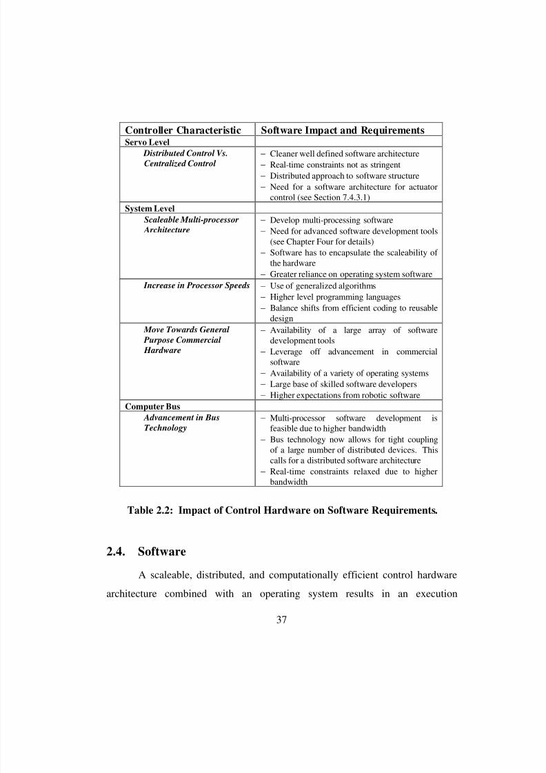
8/3/2019 Chetan Kapoor Dissertation
http://slidepdf.com/reader/full/chetan-kapoor-dissertation 61/612
37
2.4. Software
A scaleable, distributed, and computationally efficient control hardware
architecture combined with an operating system results in an execution
Controller Characteristic Software Impact and RequirementsServo Level
Distributed Control Vs.
Centralized Control − Cleaner well defined software architecture
− Real-time constraints not as stringent
− Distributed approach to software structure
− Need for a software architecture for actuatorcontrol (see Section 7.4.3.1)
System Level
Scaleable Multi-processor
Architecture− Develop multi-processing software
− Need for advanced software development tools(see Chapter Four for details)
− Software has to encapsulate the scaleability of the hardware
− Greater reliance on operating system software
Increase in Processor Speeds − Use of generalized algorithms
− Higher level programming languages
− Balance shifts from efficient coding to reusabledesign
Move Towards General
Purpose Commercial
Hardware
− Availability of a large array of softwaredevelopment tools
− Leverage off advancement in commercialsoftware
− Availability of a variety of operating systems
− Large base of skilled software developers
− Higher expectations from robotic software
Computer Bus Advancement in Bus
Technology− Multi-processor software development is
feasible due to higher bandwidth
− Bus technology now allows for tight couplingof a large number of distributed devices. Thiscalls for a distributed software architecture
− Real-time constraints relaxed due to higherbandwidth
Table 2.2: Impact of Control Hardware on Software Requirements.
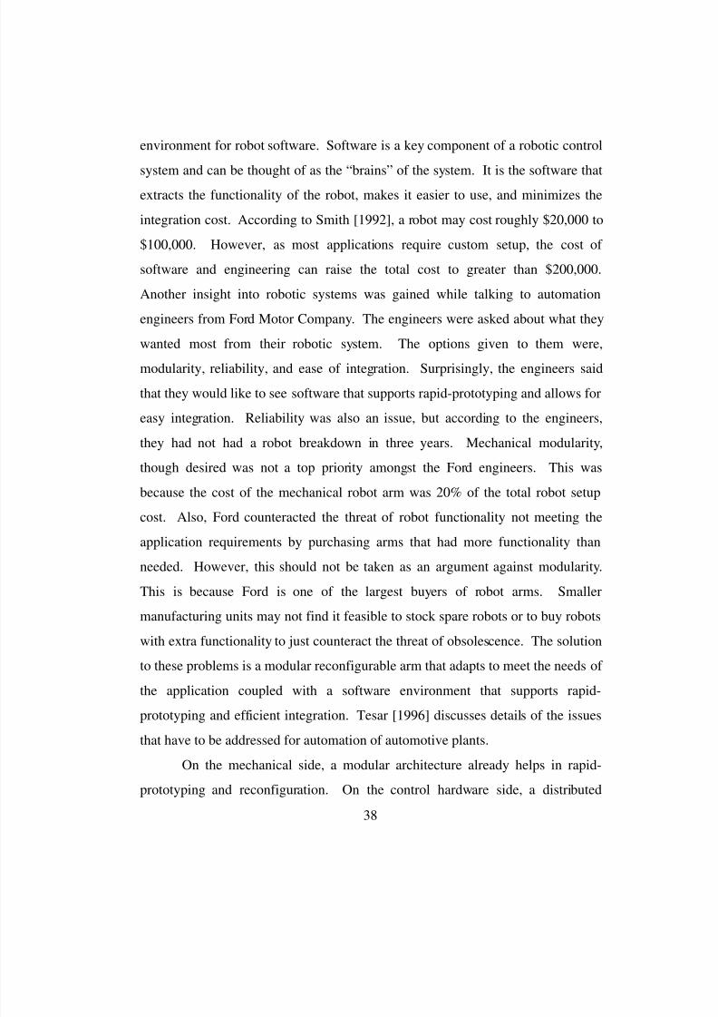
8/3/2019 Chetan Kapoor Dissertation
http://slidepdf.com/reader/full/chetan-kapoor-dissertation 62/612
38
environment for robot software. Software is a key component of a robotic control
system and can be thought of as the “brains” of the system. It is the software that
extracts the functionality of the robot, makes it easier to use, and minimizes the
integration cost. According to Smith [1992], a robot may cost roughly $20,000 to
$100,000. However, as most applications require custom setup, the cost of
software and engineering can raise the total cost to greater than $200,000.
Another insight into robotic systems was gained while talking to automation
engineers from Ford Motor Company. The engineers were asked about what they
wanted most from their robotic system. The options given to them were,
modularity, reliability, and ease of integration. Surprisingly, the engineers said
that they would like to see software that supports rapid-prototyping and allows for
easy integration. Reliability was also an issue, but according to the engineers,
they had not had a robot breakdown in three years. Mechanical modularity,
though desired was not a top priority amongst the Ford engineers. This was
because the cost of the mechanical robot arm was 20% of the total robot setup
cost. Also, Ford counteracted the threat of robot functionality not meeting the
application requirements by purchasing arms that had more functionality than
needed. However, this should not be taken as an argument against modularity.
This is because Ford is one of the largest buyers of robot arms. Smaller
manufacturing units may not find it feasible to stock spare robots or to buy robots
with extra functionality to just counteract the threat of obsolescence. The solution
to these problems is a modular reconfigurable arm that adapts to meet the needs of
the application coupled with a software environment that supports rapid-
prototyping and efficient integration. Tesar [1996] discusses details of the issues
that have to be addressed for automation of automotive plants.
On the mechanical side, a modular architecture already helps in rapid-
prototyping and reconfiguration. On the control hardware side, a distributed

8/3/2019 Chetan Kapoor Dissertation
http://slidepdf.com/reader/full/chetan-kapoor-dissertation 63/612
39
control approach combined with a scaleable architecture and standard
communication bus types helps in rapid-prototyping. The remaining technology
that needs enhancements to support rapid-prototyping is software. Software now
needs to be addressed as a commodity that can be bought off-the-shelf,
assembled, modified, and reused. The examples given in the previous paragraph
assert this need. The need for standardized reusable software components is even
greater for advanced robotics because there software is going to be larger and
more complex. The examples (Ford Motor Company and Smith) given in the
previous paragraphs were based on standard industrial robots, that is, monolithic
mechanical arms with six DOF. Software cost is going to be even higher for
advanced robots. Thus, what is needed is a development effort into the design
and testing of operational software modules for advanced robotics. A preliminary
listing of some of the required software modules for advanced robot control is
given in Table 2.3 [Tesar, 1993]. The modules are broken down into components
for actuator level control and for system level control.
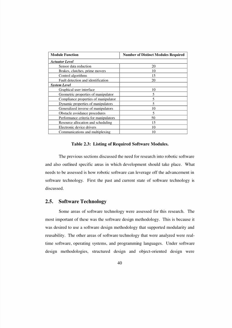
8/3/2019 Chetan Kapoor Dissertation
http://slidepdf.com/reader/full/chetan-kapoor-dissertation 64/612
40
The previous sections discussed the need for research into robotic software
and also outlined specific areas in which development should take place. What
needs to be assessed is how robotic software can leverage off the advancement in
software technology. First the past and current state of software technology is
discussed.
2.5. Software Technology
Some areas of software technology were assessed for this research. The
most important of these was the software design methodology. This is because it
was desired to use a software design methodology that supported modularity and
reusability. The other areas of software technology that were analyzed were real-
time software, operating systems, and programming languages. Under software
design methodologies, structured design and object-oriented design were
Module Function Number of Distinct Modules Required
Actuator Level
Sensor data reduction 20
Brakes, clutches, prime movers 10
Control algorithms 15
Fault detection and identification 20
System Level
Graphical user interface 10
Geometric properties of manipulator 5
Compliance properties of manipulator 5
Dynamic properties of manipulators 5
Generalized inverse of manipulators 10
Obstacle avoidance procedures 5Performance criteria for manipulators 50
Resource allocation and scheduling 15
Electronic device drivers 10
Communications and multiplexing 10
Table 2.3: Listing of Required Software Modules.
8/3/2019 Chetan Kapoor Dissertation
http://slidepdf.com/reader/full/chetan-kapoor-dissertation 65/612
41
explored. Under operating systems, standard operating systems like UNIX and
Windows NT were explored. Realizing the limitations of these operating
systems, real-time operating systems were analyzed. Programming languages
were analyzed keeping in mind their support for modular design (see Section
4.2.2).
2.5.1. Software Design
Mature industries like manufacturing are characterized by the presence of
component industries. For example, an automobile is made up of various sub-
systems, where each sub-system could possibly be supplied by a different vendor.
This is also the case for computer hardware. The software industry, which has
become a significant wealth generator, has a minimal component industry. This is
essentially due to the inherent complexity of software, lack of standardization, and
lack of a unifying software design paradigm.
The following paragraphs discuss the two predominant software design
techniques (structured and object-oriented). Of these, object-oriented design may
very well provide a solution to some of the problems faced by those developing
software for intelligent machines.
2.5.1.1. Structured Design
Since the advent of computer technology, there has been a shift from
programming-in-the-small to programming-in-the-large. The software industry
has also seen the evolution of high order programming languages. Various
software design methodologies have also evolved in the past. Of these, the most
popular is structured design. This design paradigm is also known as functional
design and procedural design. The structured design paradigm uses algorithmic
decomposition to specify tasks to be completed in order to solve a problem. This

8/3/2019 Chetan Kapoor Dissertation
http://slidepdf.com/reader/full/chetan-kapoor-dissertation 66/612
42
design methodology is typically characterized by procedural languages like C and
Pascal. Structured design relies heavily on data flow, where data flows from one
procedure (sub-routine) to another, thereby undergoing transformations. Thus, a
task is divided into procedures, and each procedure is further sub-divided. This is
also known as top-down structured design [Yourdon, 1979].
In structured design, data and instructions are kept separate. Data flows
from one sub-routine (set of instructions) to another and undergoes
transformation. For example, in robot path planning, the data corresponding to
end-effector position can be changed to joint position data by applying the inverse
kinematics sub-routine to it. This style of programming is illustrated in Figure 2.8
[Booch, 1994].
2.5.1.2. Object-Oriented Design
The other key software design methodology that is rapidly gaining
popularity is the object-oriented design. This design methodology professes that
software systems should be modeled as a collection of cooperating objects,
treating individual objects as instances of a class within a hierarchy of classes.
Input Data Output Data
Interface
Procedure
Interface
Procedure
Interface
Procedure
Figure 2.8: Structured Program Design.

8/3/2019 Chetan Kapoor Dissertation
http://slidepdf.com/reader/full/chetan-kapoor-dissertation 67/612
43
Thus, the first step in the analysis of the problem domain using object-oriented
techniques involves identifying the key objects that make up the system. Objects
with similar characteristics are part of an inheritance structure that is used to
extract the benefits of commonality. Each object has a standard interface through
which it communicates with other objects. Additionally, each object contains its
own functionality. This is similar to the way physical systems and entities exist.
As a result of this similarity, the structure of an object-oriented software ends up
resembling that of the physical problem domain [Booch, 1994]1. Five General
concepts of object-oriented design are discussed in the following section. These
are, classes, data abstraction, inheritance, polymorphism, and dynamic binding.
The first three appear in high level design and analysis. The last two are added
during low-level design and implementation [Korson and McGregor, 1990].
2.5.1.2.1. Classes
Classes in object-oriented design are used to define a group of objects with
similar characteristics. This can be explained best by a real world example. A
can (food packaging) class can be defined that would include all sorts of cans
ranging from soda cans to paint cans. When the can class is defined, the designer
has to define the interface to this class. This means deciding what is visible to the
user. For example, for the can class, the interface could consist of a function
which returns the capacity of the can (get_capacity) and another function which
returns the contents of the can (get_contents). These functions (called methods in
object-oriented design) would be implemented as an integral part of the can class
and will be visible from outside the class. These visible methods are known aspublic methods. Other methods are also defined by the designer which are used to
1 In the past procedural design and software parallelism was used to structure software. Object-

8/3/2019 Chetan Kapoor Dissertation
http://slidepdf.com/reader/full/chetan-kapoor-dissertation 68/612
44
calculate data which is needed by the public methods. For example, a method can
be implemented which calculates the volume (calculate_volume) of the can. The
output of the calculate_volume method will be used by the get_capacity method.
Thus, there would be no real need for exposing the calculate_volume method to
the user. In other words, calculate_volume can be made a private method of the
can class. Thus, by implementing a method as a private member, the software
designer makes sure that it is not visible to the world outside the class. This
technique of hiding data is called encapsulation and is used for data abstraction.
Data abstraction will be discussed in more detail in the next section.
Besides having public and private methods there are two other constructs
which are a part of the class and are used in object-oriented design. In C++ these
are called the constructor and destructor . A constructor is used to create an
instance of a class. This instance is also known as an object. The can analogy is
referred to again to explain instantiation. In the real world, when a can is
designed on paper, the designer lays out the characteristics of the can. These
characteristics would be general purpose rules which would define the behavior of
a can. When a can gets manufactured and gets a distinct identity (example, a
Coke can) it is called an object. Thus, from the can class defined above, different
objects of the type can, can be instantiated. These objects can have different
capacities and contents. An implementation of the can class in pseudo code is
shown below:
Class can{
public methods:
constructor(...........);
destructor(..............);get_capacity(.........);
get_type_of_contents(.........);
oriented design now offers another means of defining software structure.
8/3/2019 Chetan Kapoor Dissertation
http://slidepdf.com/reader/full/chetan-kapoor-dissertation 69/612
45
private methods:
calculate_volume(....);evaluate_content_type(.......);
}
In object-oriented design when an entity of a particular class type is
created, it is called an object. For example, from the can class if a can with a
volume 20cc and contents soda is created, it will be called an object. These
objects form the basic run-time entities in an object-oriented system. Objects take
up space in memory and have an associated address like a data type in FORTRAN
and C. Associated with every object is a set of methods that define the
meaningful operations on that object. In traditional procedural programming a
new data type can be defined but the methods which act on this data type are
separate and are in the form of sub-routines.
The destructor used in C++ is used to deallocate the memory allocated to
an object and thus stop its existence.
A more related example of a class would be a matrix class. The matrix
class in all probability will have public methods for multiplication, inversion, and
transposing. There can be some private methods for doing memory management
and other methods implementing different matrix inversion techniques. The
implementation of the matrix class would look somewhat as shown:
Class matrix{
public methods:
constructor(row, column);
destructor(..............);
invert(.........);multiply(.........);
add(..........);
transpose(.........);
private methods:
8/3/2019 Chetan Kapoor Dissertation
http://slidepdf.com/reader/full/chetan-kapoor-dissertation 70/612
46
adjoint(.......);
set_up_sparse_matrix(........);
private data:real A[i][j];
}
Instantiation of an object of type matrix would be similar to instantiating a
simple integer. For example, the statement “matrix B;” would create an object
‘B’ of type matrix. All the methods shown in the matrix class above would be a
part of the object ‘B.’
2.5.1.2.2. Data Abstraction
Various abstraction mechanisms are available in programming languages.
Procedural abstraction, for example, is based on parameterizing a programming
unit (sub-routine), that is, allowing the same processing steps to be applied to
different data. Data abstraction, on the other hand, separates the behavior of a
data type from its implementation. Users of the data type see only its external
view (that is the set of operators), allowing its implementation to be modified
without adverse effects. This data hiding is known as encapsulation. To fully
encapsulate a data type, operators on it must be adequate, that is, they must be
fully capable of constructing, observing, and (possibly) modifying instances of a
data type [Korson and McGregor, 1990]. An example of an Abstract Data Type
(ADT) is the matrix class. To the user what is visible is the interface to the
methods (multiplication, inversion, transposing) embedded in the class (see
Figure 2.9).
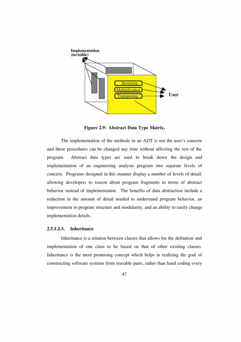
8/3/2019 Chetan Kapoor Dissertation
http://slidepdf.com/reader/full/chetan-kapoor-dissertation 71/612
47
Inversion
Multiplication
Transposing User
Implementation(invisible)
Figure 2.9: Abstract Data Type Matrix.
The implementation of the methods in an ADT is not the user’s concern
and these procedures can be changed any time without affecting the rest of the
program. Abstract data types are used to break down the design and
implementation of an engineering analysis program into separate levels of
concern. Programs designed in this manner display a number of levels of detail,
allowing developers to reason about program fragments in terms of abstract
behavior instead of implementation. The benefits of data abstraction include a
reduction in the amount of detail needed to understand program behavior, an
improvement in program structure and modularity, and an ability to easily change
implementation details.
2.5.1.2.3. Inheritance
Inheritance is a relation between classes that allows for the definition andimplementation of one class to be based on that of other existing classes.
Inheritance is the most promising concept which helps in realizing the goal of
constructing software systems from reusable parts, rather than hand coding every
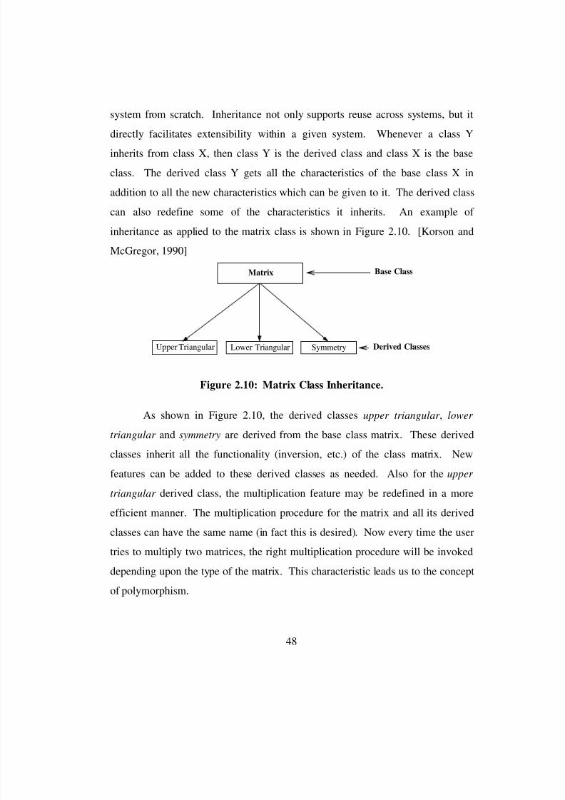
8/3/2019 Chetan Kapoor Dissertation
http://slidepdf.com/reader/full/chetan-kapoor-dissertation 72/612
48
system from scratch. Inheritance not only supports reuse across systems, but it
directly facilitates extensibility within a given system. Whenever a class Y
inherits from class X, then class Y is the derived class and class X is the base
class. The derived class Y gets all the characteristics of the base class X in
addition to all the new characteristics which can be given to it. The derived class
can also redefine some of the characteristics it inherits. An example of
inheritance as applied to the matrix class is shown in Figure 2.10. [Korson and
McGregor, 1990]
Matrix
Upper Triangular Lower Triangular Symmetry
Base Class
Derived Classes
Figure 2.10: Matrix Class Inheritance.
As shown in Figure 2.10, the derived classes upper triangular , lower triangular and symmetry are derived from the base class matrix. These derived
classes inherit all the functionality (inversion, etc.) of the class matrix. New
features can be added to these derived classes as needed. Also for the upper
triangular derived class, the multiplication feature may be redefined in a more
efficient manner. The multiplication procedure for the matrix and all its derived
classes can have the same name (in fact this is desired). Now every time the user
tries to multiply two matrices, the right multiplication procedure will be invoked
depending upon the type of the matrix. This characteristic leads us to the concept
of polymorphism.
8/3/2019 Chetan Kapoor Dissertation
http://slidepdf.com/reader/full/chetan-kapoor-dissertation 73/612
49
2.5.1.2.4. Polymorphism
In general, polymorphism means the ability to take more than one form.In an object-oriented language, a polymorphic reference is one that can, over time,
refer to instances of more than one class. Polymorphism allows the user to have
functions with the same name. For example, if actuator joint position data is
desired from a robot controller, the applications writer has to just call the function
get_position_data. The device which is delivering the data can be a tachometer, a
resolver or a potentiometer. All these devices will probably be represented as
derived classes of a base class called position_devices.
Polymorphism allows operator overloading. Under this the operators (e.g.
+, -, *, etc.) can be redefined to act on other data types besides integers and reals.
In an application to the matrix class, the operator ‘+’ can be overloaded to act as
an operator for matrix addition.
2.5.1.2.5. Dynamic Binding
The binding referred to in this section is the binding of a procedure call to
the code to be executed in response to the call. Dynamic binding means the code
associated with a given procedure call is not known until the moment of the call at
runtime. For example, the multiplication procedure call for the class matrix is
dynamically bound to a particular multiplication procedure depending upon the
derived class of matrix which is requesting this procedure. Inheritance is
successfully used by incorporating dynamic binding. For example, consider a
software architecture for position sensors. In this architecture, there is a software
component called PositionSensor and two other components named Encoder and
Resolver that are derived from PositionSensor . All these components have
functionality for reading the position. Let this method be known as GetPosition.
When the GetPosition method is called by the user, the correct functionality for
8/3/2019 Chetan Kapoor Dissertation
http://slidepdf.com/reader/full/chetan-kapoor-dissertation 74/612
50
accessing the position will automatically be called (or dynamically bound) based
on the type of the PositionSensor (that is, Encoder or Resolver ). The user of this
architecture has to only familiarize themselves with the interface provided by the
PositionSensor component. Future users of this architecture can add other
position sensors. The control program that was written using the PositionSensor
interface will simply incorporate the change in the position sensor with minimal
source code changes. This characteristic of object-oriented design allows
designers to develop programs at an abstract level
2.5.1.3. Object Oriented Support for Good Design
Object-oriented design inherently supports (and enforces) some of the
characteristics of a good design. These are modularity, information hiding, weak
coupling, extensibility, and integrability. These are discussed below:
Modularity: The object-oriented paradigm provides natural support for
decomposing a system into modules. In this paradigm classes are the modules.
This means that not only the design process supports modularity, but the
implementation process supports it as well through the class definition. [Korson
and McGregor, 1990]
Information Hiding: The class constructs support information hiding
through the separation of the class interface and the class implementation. The
separation allows the class interface to be mapped to several different
implementations. It also allows much maintenance activity to be hidden from
users of the class. For example, the implementation of the inversion procedure of
the matrix class can be hidden from the user. [Korson and McGregor, 1990]Weak Coupling: Classes are designed as collections of data and the set
of allowable operations on the data. Therefore, the interface operators of a class
are inward-looking in the sense that they are intended to access or modify the

8/3/2019 Chetan Kapoor Dissertation
http://slidepdf.com/reader/full/chetan-kapoor-dissertation 75/612
51
internal data of the class. This leads to fewer connections between the classes.
[Korson and McGregor, 1990]
Extensibility: The object-oriented paradigm produces designs that are
easily extended. The inheritance mechanism supports extending designs in two
ways. First, the inheritance relation facilitates the reuse of existing definitions to
ease the development of new definitions. As the inheritance structure becomes
progressively deeper, the amount of specification and implementation inherited by
new class definition grows. This usually means that as the inheritance structure
grows, the amount of effort to develop a new class decreases. Second, the
polymorphic property of the typing system in object-oriented languages also
supports extensible designs. [Korson and McGregor, 1990]
Integrable: The object-oriented design process produces designs which
facilitate the integration of individual pieces into complete designs. The narrow,
clearly defined interface of a class supports integration with other software
components. The narrow interface corresponds naturally to the observable
behaviors of the real-world entity modeled by the class. The interfacing of two
classes then is as a model of the natural interaction of the two entities. [Korson
and McGregor, 1990]
Over structured design, object-oriented design offers the advantages of
modularity, encapsulation, standard interfaces, abstraction, reuse, extensibility,
and maintainability [Booch, 1994][Champeaux et al., 1992]. The object-oriented
programming paradigm is commonly identified by programming languages like
C++, SmallTalk, Ada, ObjectPascal, Lisp, etc. Of all these languages, C++ has
gained much popularity. This is primarily due to its design features and
compatibility with the C programming language [Jordan, 1990] (see Section 4.2.2
for details). Booch [1994] outlines some of the applications that can benefit from
object-oriented program design. Some of these are listed below. The

8/3/2019 Chetan Kapoor Dissertation
http://slidepdf.com/reader/full/chetan-kapoor-dissertation 76/612
52
technologies that directly affect advanced robotics and could benefit from object-
oriented design are highlighted.
• Air traffic control • Animation
• Avionics • Banking and insurance software
• Business data processing • Chemical process control
• Command and control systems • Computer aided design
• Computer aided education • Petroleum engineering
• Computer integrated
manufacturing
• Software development
environments
• Expert systems • Hypermedia
• Image recognition and vision • Mathematical analysis
•
Medical electronics •
Office automation• Operating systems • Reusable software components
• Robotics • Databases
• Space station software • Spacecraft and aircraftsimulation
• Telecommunications • Telemetry systems
• User interface design • VLSI design
Various analysis and design techniques for object-oriented software
development have been proposed by researchers. Based on requirements and user
preferences, an analysis and design methodology can be chosen [Booch, 1994][Shlaer and Mellor, 1988]. However, all these design methodologies agree on a
basic three-phase life cycle for software development: 1) analysis, 2) design, and
3) implementation. The analysis phase covers the initiation of the project through
to user’s-need analysis and to a feasibility study. The design phase covers the
various concepts of the system design, broad design, logical design, detailed
design, program design, and physical design. After the completion of the design
phase the software enters the implementation phase. The whole process is
iterative, and there is communication back-and-forth between each design phase
[Henderson-Sellers and Edwards, 1990].
8/3/2019 Chetan Kapoor Dissertation
http://slidepdf.com/reader/full/chetan-kapoor-dissertation 77/612
53
2.5.2. Real-Time Software
The implementation of robot control software is essentially a problem inthe domain of real-time computing. Fault-tolerance adds a new challenge to real-
time software as it addresses the need for deterministic software techniques for
fault detection and recovery. Real-time software is characterized by a system that
not only produces logically correct results, but also produces them in a timely and
deterministic manner. It is a common misconception that “if it is fast enough it is
real-time.” Speed of execution, though a critical requirement, is not the only
characteristic of a real-time system. A real time system should be able to respond
to external events efficiently without violating the temporal constraints associated
with such a system. The external events can be of the following types:
• multiple asynchronous external events,
• multiple cyclical external events, or
• a combination of the above [Stankovic, 1988].
Real time software can be designed in different ways with the main
purpose to respond to external events in a timely fashion. These approaches are
the ad hoc style and the multitasking approach. These approaches are discussed
in the following sections.
2.5.2.1. Ad Hoc Approach
In the ad hoc style of developing real time software, the software is
designed to function in the form of a loop. As the software goes through the loop,
it services each external event and performs calculations. This is illustrated in
Figure 2.11.
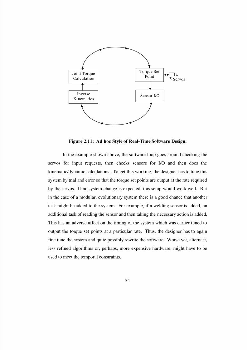
8/3/2019 Chetan Kapoor Dissertation
http://slidepdf.com/reader/full/chetan-kapoor-dissertation 78/612
54
Joint TorqueCalculation
InverseKinematics
Sensor I/O
Servos
Torque SetPoint
Figure 2.11: Ad hoc Style of Real-Time Software Design.
In the example shown above, the software loop goes around checking the
servos for input requests, then checks sensors for I/O and then does the
kinematic/dynamic calculations. To get this working, the designer has to tune this
system by trial and error so that the torque set points are output at the rate required
by the servos. If no system change is expected, this setup would work well. But
in the case of a modular, evolutionary system there is a good chance that another
task might be added to the system. For example, if a welding sensor is added, an
additional task of reading the sensor and then taking the necessary action is added.
This has an adverse affect on the timing of the system which was earlier tuned to
output the torque set points at a particular rate. Thus, the designer has to again
fine tune the system and quite possibly rewrite the software. Worse yet, alternate,
less refined algorithms or, perhaps, more expensive hardware, might have to be
used to meet the temporal constraints.
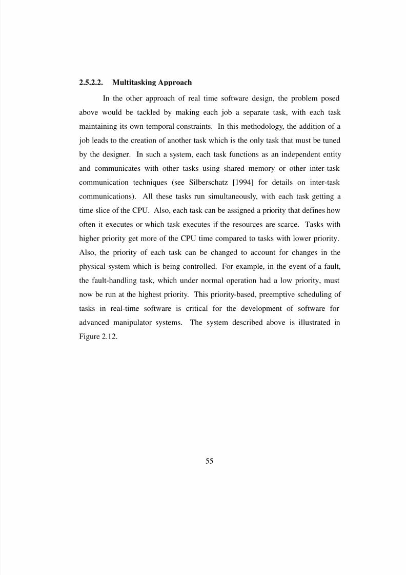
8/3/2019 Chetan Kapoor Dissertation
http://slidepdf.com/reader/full/chetan-kapoor-dissertation 79/612
55
2.5.2.2. Multitasking Approach
In the other approach of real time software design, the problem posedabove would be tackled by making each job a separate task, with each task
maintaining its own temporal constraints. In this methodology, the addition of a
job leads to the creation of another task which is the only task that must be tuned
by the designer. In such a system, each task functions as an independent entity
and communicates with other tasks using shared memory or other inter-task
communication techniques (see Silberschatz [1994] for details on inter-task
communications). All these tasks run simultaneously, with each task getting a
time slice of the CPU. Also, each task can be assigned a priority that defines how
often it executes or which task executes if the resources are scarce. Tasks with
higher priority get more of the CPU time compared to tasks with lower priority.
Also, the priority of each task can be changed to account for changes in the
physical system which is being controlled. For example, in the event of a fault,
the fault-handling task, which under normal operation had a low priority, must
now be run at the highest priority. This priority-based, preemptive scheduling of
tasks in real-time software is critical for the development of software for
advanced manipulator systems. The system described above is illustrated in
Figure 2.12.
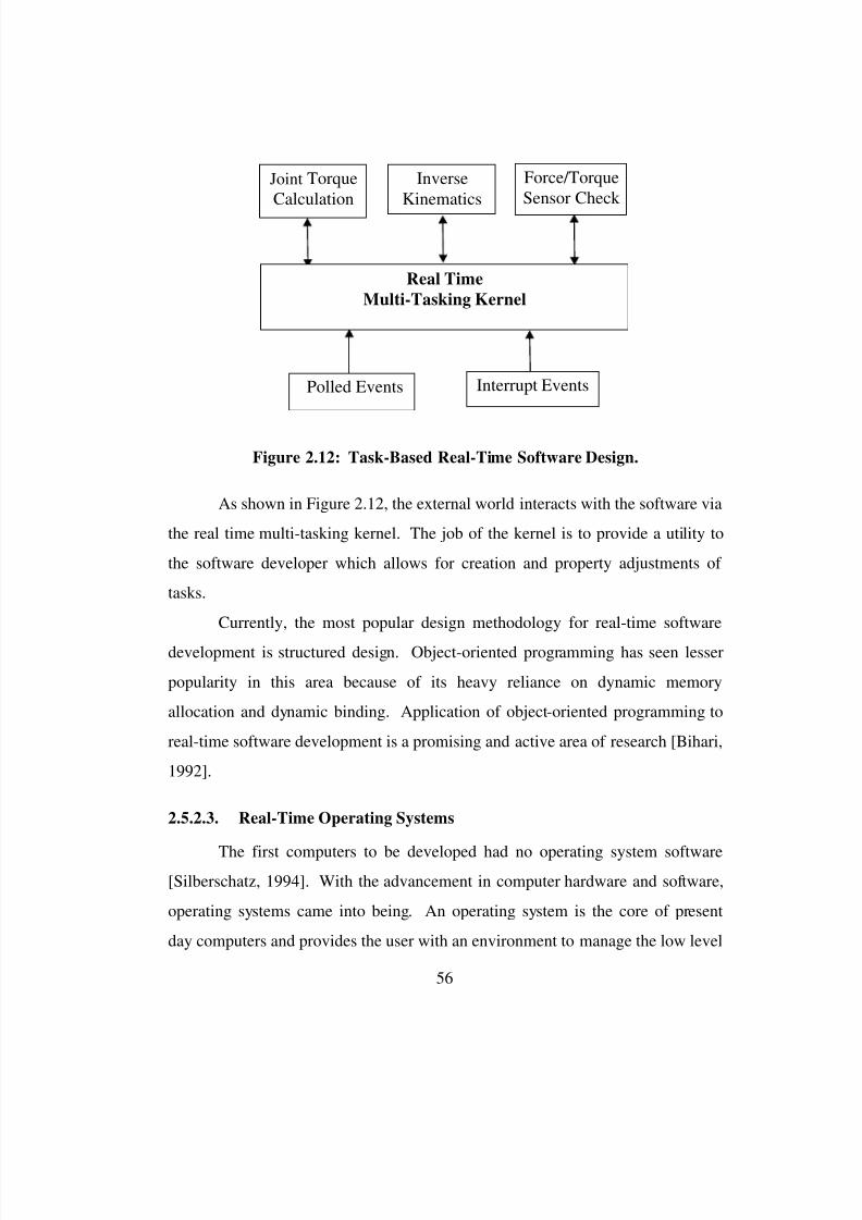
8/3/2019 Chetan Kapoor Dissertation
http://slidepdf.com/reader/full/chetan-kapoor-dissertation 80/612
56
Joint TorqueCalculation
InverseKinematics
Force/TorqueSensor Check
Real Time
Multi-Tasking Kernel
Polled Events Interrupt Events
Figure 2.12: Task-Based Real-Time Software Design.
As shown in Figure 2.12, the external world interacts with the software via
the real time multi-tasking kernel. The job of the kernel is to provide a utility to
the software developer which allows for creation and property adjustments of
tasks.
Currently, the most popular design methodology for real-time software
development is structured design. Object-oriented programming has seen lesser
popularity in this area because of its heavy reliance on dynamic memory
allocation and dynamic binding. Application of object-oriented programming to
real-time software development is a promising and active area of research [Bihari,
1992].
2.5.2.3. Real-Time Operating Systems
The first computers to be developed had no operating system software[Silberschatz, 1994]. With the advancement in computer hardware and software,
operating systems came into being. An operating system is the core of present
day computers and provides the user with an environment to manage the low level
8/3/2019 Chetan Kapoor Dissertation
http://slidepdf.com/reader/full/chetan-kapoor-dissertation 81/612
57
details of the execution of software. Some important functions of an operating
system are process management, memory management, and file system
management. Popular examples of operating systems are UNIX, Windows NT,
OS/2, etc. However, these operating systems were developed for normal program
execution rather than real-time execution of software. Thus, there was a need for
real-time operating systems that would facilitate software development for real-
time systems.
Real-time operating systems are based on the complementary concepts of
multi-tasking and inter-task communication. The various tasks that execute on a
real-time system have priorities, and a high priority task has the authority to
preempt a low priority task in the event of resource scarcity (CPU power). UNIX,
even though a multi-tasking system, does not allow preemption of processes and
thus is unsuitable for real-time software execution. However, most commercially
available UNIX systems offer kernel extensions that support the development of
real-time software [Silberschatz, 1994]. Commercially, a large number of real-
time operating systems are available for real-time software development and
execution [Landman, 1996]. The research community has also developed real-
time operating systems for specific applications. CHIMERA is a real-time
operating system developed at Carnegie Mellon University and is characterized by
a high performance real-time kernel that supports preemptive priority-based
process scheduling [Schmitz, 1989]. RCCL was a major effort in robot control
and was based on the use of UNIX for real-time control. Hayward and Paul
developed the RCCL system by modifying the UNIX kernel for real-time software
execution. On top of this system they developed a robot control C library (RCCL)
to aid the user in developing robot programs or for testing various control
algorithms [Hayward et al., 1986]. In brief, the key factors to consider in the
selection of a real-time operating system are:
8/3/2019 Chetan Kapoor Dissertation
http://slidepdf.com/reader/full/chetan-kapoor-dissertation 82/612
58
• Is the desired hardware platform supported?
•
What is the interrupt latency time (should be as small as possible)?• What is the context switch time (time to switch between tasks should be as
small as possible)?
• Are good software development tools available (compilers, linkers, debuggers,
performance analyzers, etc.)?
• Does the operating system support object-oriented software development?
• Is multi-processing (multiple CPU) supported?
•
Does the application need a kernel or a full-blown operating system?
2.6. Robotic Software Systems
Sections 2.2 and 2.3 discussed the mechanical hardware and computer
hardware technology involved in robotic systems. The third technology, a crucial
one, that is required for a successful robotic system is the operational software.
The software constitutes the ‘brains’ of the robot and can also help in balancing
some of the limitations of the mechanical and computer hardware of the system.
The design of the software system also influences the integration cost and the
usability of the robot manipulator. The following sections discuss the three major
layers of robotic systems control software and give an overview of the past and
current research in those areas. The middle layer of robotic software (operational
software) is discussed in greater detail as this research focuses on developing a
software architecture for this layer.
2.6.1. Man-Machine Interface
This is the top-most layer of robotic software and it provides means for
accessing the functionality of a robot. This layer is primarily composed of the
robot programming environment which consists of the robot programming

8/3/2019 Chetan Kapoor Dissertation
http://slidepdf.com/reader/full/chetan-kapoor-dissertation 83/612
59
language (RPL) and a graphical user interface (GUI). A majority of work done in
the past in robotics involved the development of RPLs [Banachiewicz,
1986][Blume and Jacob, 1984][Grossman, 1986][Harima and West,
1992][Lozano-Peréz, 1983][Rembold and Blume, 1985]. These languages have
continued to evolve and the level of abstraction provided by them continues to
increase with the advancement in computer technology. This has led to the
evolution of RPLs from simple interpreted languages to structured languages to
languages that support task-level programming. Currently, there is no standard
for robot programming languages. In addition to specifically developed RPL’s,
commercially available general purpose languages have also been used for robot
programming. For example, C, Ada, SmallTalk, and Basic have been used for
robot programming [Cox and Gehani, 1987][Hayward and Paul, 1986][LaLonde
et al., 1987][Mohri et al., 1985][Volz et al., 1983]. Also, graphical interfaces
have been developed on top of robot programming languages to assist in robot
programming [Chen et al., 1992][Kapoor, 1992][Smith, 1992]. Current industrial
robot programming techniques use a teach pendant and a RPL to program a robot.
This technique is cumbersome and requires continuous re-teaching of points by
the operator [Leu, 1985]. Task-level robot programming is an evolving technique
that relies on sensor integration and is based on artificial intelligence. In task-
level robot programming, the robot task is specified at a fairly high level of
abstraction as opposed to manipulator level programming where the robot
program is in terms of robot states [Lozano-Peréz, 1983].
2.6.2. Operational Software
A robot programming language is the top most layer of the robotic
software. The layer of software that actually translates the robot programming
language constructs into actuator commands is called the operational software
8/3/2019 Chetan Kapoor Dissertation
http://slidepdf.com/reader/full/chetan-kapoor-dissertation 84/612
60
layer. This layer includes kinematics, dynamics, deflection modeling, criteria-
based decision making, and fault-tolerance. Current industrial robots fail to
implement the operational software layer in its full complexity [Tesar, 1989].
Moreover, the software for current robotic systems is implemented as a closed-
system: a system that does not allow for user modification and extension.
Additionally, as most industrial robots are non-reconfigurable six DOF wrist-
point arms, they have simplified kinematics. As such, most of these robots
implement a closed-form inverse kinematics solution and a simplified dynamics
model. None of these formulations are generalized and scaleable [Tesar, 1989].
Thus, what is needed is an operational software architecture for advanced robots.
This architecture will provide the user with basic building blocks which can
be used to develop control programs for robots. These software components
should be reusable. That is, the components should be general enough to
apply to different robots and also be user modifiable and extensible.
Additionally, these components should be applicable to real-time control and
simulation.
The following sections give a detailed literature review of efforts at
developing robotic software systems. Most of the systems discussed implement
all three layers of robotic software and in general have a nominal operational
software layer.
2.6.2.1. RCCL (Robot Control C Libraries)
The Robot Control C Libraries (RCCL) was a significant effort in the
development of a robot control and programming environment based on a UNIXworkstation and the C programming language [Hayward and Paul, 1986]. The
current implementation of this system includes a world modeler, a trajectory
generator, a graphical simulator, and multiple robot support. However,

8/3/2019 Chetan Kapoor Dissertation
http://slidepdf.com/reader/full/chetan-kapoor-dissertation 85/612
61
generalized kinematics, deflection modeling, and support for reconfigurable robot
arms is missing from RCCL. Overall, RCCL is one of the most comprehensive
environments for robotics research, but it lacks in key capabilities such as fault-
tolerance, redundancy, and decision making. From a software point of view,
RCCL is based on structured design and thus does not provide the benefits of
reuse via extensibility, which are the hallmark of object-oriented software. Also,
a major effort in RCCL was spent in modifying UNIX for real-time control.
Currently, most commercially available operating systems already support real-
time extensions.
2.6.2.2. Robot Independent Programming Environment (RIPE)
Current trends exhibit the increasing application of object-oriented
software techniques to the development of robotic systems. Miller and Lennox
[1991] at Sandia National Labs have developed a robot independent programming
environment. This software environment uses C++ as the implementation
language, and has the benefits of modularity, abstraction, and extensibility. This
environment allows for rapid-prototyping of robot workcells and provides the user
with a standard interface with which various robots can be programmed. RIPE
interfaces with robot system controllers at the host level. However, RIPE is a
robot programming environment. It does not provide a framework for robotics
research in the areas such as generalized kinematics, decision making, and fault-
tolerance.
2.6.2.3. Generic Intelligent System Control (GISC)
GISC is an effort by Sandia National Labs at developing an open
architecture for machine control [Burchard and Feddema, 1996]. Based on the
GISC-kit a generic robotic and motion control Applications Programming
8/3/2019 Chetan Kapoor Dissertation
http://slidepdf.com/reader/full/chetan-kapoor-dissertation 86/612
62
Interface (API) has been developed. This API provides a generic interface for
command sequences between a supervisory control system and devices ranging
from one DOF motion devices up to six DOF robotic systems. This API can be
used for distributed control. Communication across different platforms (UNIX,
PC’s) is achieved using an object brokerage system (in this case the CORBA
software). The GISC software system further relies on RIPE to interface with
robot system controllers. The combination of GISC and RIPE offers a
sophisticated environment for machine interfacing using the latest in software
technology. However, these systems do not address the operational software
needs of advanced robots. These systems are merely used for supervisory control.
Additionally, GISC and RIPE have been used to interface to standard six DOF
industrial robots. These robots are mechanically constrained and require a
minimal operational software layer.
2.6.2.4. Sequential Modular Architecture for Robotics and Teleoperation
Sequential Modular Architecture for Robotics and Teleoperation
(SMART) is an effort by Sandia National Laboratories at developing a software
environment that supports the building of complex nonlinear digital robot control
systems from modular components that guarantee stability and predictable
performance [Anderson, 1993]. SMART has been applied to projects as diverse
as multi-robot control, flexible robot simulation, kinesthetic virtual reality, and
11-DOF redundant robot control. SMART incorporates over a hundred different
modules that include sensors, input devices, and robots. Modules that include the
computation of kinematics and dynamics are also available.SMART can be used for any robot that can accept external position set
points and with any sensor that can be interfaced to a VME bus. Distinct modules
are defined for each sensor, actuator, input device, and dynamic element. The
8/3/2019 Chetan Kapoor Dissertation
http://slidepdf.com/reader/full/chetan-kapoor-dissertation 87/612
63
hardware consists of commercially available CPUs and processor boards running
on a VME bus with a UNIX-based operating system like VxWorks. The system
is connected to a host processor and a graphics workstation by Ethernet. The
software consists of libraries of C routines. The architecture is parallel and real-
time.
From the literature reviewed, it is clear that SMART is the only robotic
software environment that comes close to achieving the goals of the OSCAR
architecture that is being proposed in this research. However, SMART is a real-
time generic control architecture that has some operational software content. This
research will focus on the operational software and develop a reusable
architecture for that purpose. Additionally, SMART is available as a library of C
routines. This implies limited object-oriented capability of SMART.
2.6.2.5. Control Shell
Control shell is a component-based real-time programming system. This
system is based on object-oriented design and it provides components that allow
the building of real-time control systems. Control shell further provides a
graphical environment for assembling the components. New components can also
be created by aggregating the existing components. Reusable components are
provided for PID control, impedance control, and trajectory generation. Control
shell also supports a network transit system. This system uses Ethernet and TCP
sockets for communication [Brain, 1994]. Further, control shell supports run-time
configuration management. This allows the run-time reconfiguration of the
execution structure. For example, a PID controller could be replaced by a PDcontroller to quickly get a comparison. Control shell is based on the VxWorks
real-time operating system [WindRiver Systems] and it bridges the gap between
VxWorks and the real-time application. [Schneider et al., 1994]
8/3/2019 Chetan Kapoor Dissertation
http://slidepdf.com/reader/full/chetan-kapoor-dissertation 88/612
64
Basically, control shell addresses all the issues involved in robotic system
level software. However, control shell has a minimal operational software layer.
Support for advanced robotics is completely missing. It does, however provide a
framework for further robotic software development. The operational software
layer being developed as a part of this research could be integrated with control
shell. This would make control shell applicable to advanced robotics.
2.6.2.6. Robot Shell
An effort by Vuskovic et al. [1988] led to the development of a robotic
application-oriented extension to the UNIX shell, called the robot shell. This
provided support for general purpose formulations related to robotics. This
includes homogenous transformation matrices, three-by-three rotation matrices,
vectors, various orientation angle representations, etc. Using the robot shell, the
user could model robotic systems efficiently. However, support for generalized
kinematics, dynamics, deflection compensation, fault-tolerance, etc. was missing.
Moreover, commercial tool-kits can be purchased as extensions to mathematical
software (example Matlab and Mathematica) which provide robotic related
constructs. An advantage of the robot shell is that it provides an interactive
environment. This allows for quick evaluation of results and testing of simple
algorithms. A compiled software environment is better suited for complex
algorithms which have real-time constraints. This is because various
optimizations can be done by the compiler and the user has more control over the
data flow in the program.
2.6.2.7. Design Automation
Effort in mechanical design software has also been concentrated in the
development of new programming languages suited for mechanical design. The
8/3/2019 Chetan Kapoor Dissertation
http://slidepdf.com/reader/full/chetan-kapoor-dissertation 89/612
65
latest among this is the CH programming language that is designed to be a
superset of ISO C with incorporation of all the programming features of
FORTRAN 90 [Cheng, 1995]. CH supports metanumbers (-0.0, +0.0, Inf, -Inf,
and Nan) and provides data types for complex, dual, and array. Besides these
features, the language supports polymorphism that allows for different functions
to have the same name with different argument types. Also CH borrows the
syntax of call-by-reference from C++. CH
also supports nested functions which
are beneficial for encapsulation and hence modularity. CH supports automatic
type conversion. An example of this is when a real number is automatically type-
casted to a complex. Automatic type conversion is a serious design issue and is
generally undesirable for robust software development [Coplien, 1994]. However
a controlled use of automatic type conversion can ease the software development
process. C++ is a strongly typed language but it allows the implementation of
automatic type conversion between data types. All the features of CH are
available or can be made available in C++. Nested functions can be represented
in C++ by using block-structured programming techniques [Coplien, 1994]. The
metanumbers can be implemented as data types by encapsulating the underlying
representation of floats and doubles in C++. Also, the complex, dual, and array
data types are rudimentary and are straight-forward to implement in C++. In
addition, due to the object-oriented nature of C++, these data types, when
implemented will have the look and feel of built-in data types to the user.
Moreover, C++ being an object-oriented language, it allows for reuse and
extensibility through dynamic binding, inheritance, and parameterized types
[Coplien, 1994]. A novice does not have to use these advanced features and can
be satisfied by the data types provided. However, an advanced user can extend
these data types, modify them, and create new ones. This capability is essential
for building large scale software systems for intelligent machines.
8/3/2019 Chetan Kapoor Dissertation
http://slidepdf.com/reader/full/chetan-kapoor-dissertation 90/612
66
2.6.2.8. Various Object-Oriented Robotic Environments
Tomiyama et al. [1991] were involved in the development of a UNIX-based robot control system. In this, the real-time computations are done on
Motorola 68020 CPU boards on a VME backplane. The UNIX workstation is a
host computer that is used for software development and to provide an interface to
the operator. This architecture is fairly standard and is commonly used in today’s
research environments [Aalund, 1991]. Again, this setup was for one particular
robot arm and the software developed for this endeavor was not generalized
enough to take care of other robot arms.
Object-oriented techniques have been applied to robotics research in
excavation, sensor integration, manufacturing cell control, and predominantly
robot programming and motion planning. Zheng’s [1989] effort at sensor
integration utilizes object-oriented design to create the concept of a logical sensor.
Using this approach, a sensor is modeled at a high level of abstraction as an
abstract data type. This allows for a software architecture which does not change
as sensors are added, removed or modified. The sensor integration takes place in
all three layers of robotic software and does not modify the overall structure of the
software.
Baugh and Rehak [1992] outline the advantages of data abstraction in the
development of engineering software. According to them, data abstraction offers
the advantages of modularity and provides a clean delineation between design and
implementation. Again, object-oriented design languages are proposed as they
best support the linguistics for data abstraction.
Work was done by Bullock and Oppenhiem [1992] in developing an
object-oriented software system for robotics research in excavation. Again the
characteristics of modularity, standardized interfaces and data abstraction that are
8/3/2019 Chetan Kapoor Dissertation
http://slidepdf.com/reader/full/chetan-kapoor-dissertation 91/612
67
offered by object-oriented design lead to a computational environment that
supports rapid-prototyping.
All robot manipulators have a definite sequence of steps through which
they are powered-on and powered-off. Cox [1988] used the constructor and
destructor mechanism to develop a robotic software system that supports
guaranteed initialization and safe termination. This leads to a more reliable
system. Additionally, C++ support for exception handling is used for safe error
recovery and termination.
Pimentel [1990] used an object-oriented software architecture for
specifying, designing, coding, and testing software for intelligent automation
systems. This system was primarily for supervisory control of machines and did
not deal with the operational software aspects of the machine (robot).
Nevertheless, object-oriented design led to a more modular and scaleable
environment with standardized interfaces.
Currently, robotics research has focused on using object-oriented software
design to implement robot planning and programming systems. Work done by
Boyer et al. [1991] led to the development of a Dual-Hierarchical Object-Oriented
Design (DHOOD) methodology. This methodology modifies the standard
methodology of object-oriented design (which involves identifying relevant
physical objects and mapping them into object classes) to include support for
concurrency and distributed software systems. Concurrency is important for robot
planning software due to the asynchronous and parallel nature of the physical
environment which the software is supposed to control. The work done by Bison
and Gini [1989] provides an argument for using object-oriented programming for
task-level robot programming. The ability to construct self-contained modules
and to interact with them at a high level of abstraction lends itself to task-level
robot programming.
8/3/2019 Chetan Kapoor Dissertation
http://slidepdf.com/reader/full/chetan-kapoor-dissertation 92/612
68
2.6.2.9. Summary of the Operational Software Literature Review
This section discussed some relevant work done in the development of robotic software systems that have some operational software content. It was seen
that most of these systems were developed for standard six DOF industrial robots.
The operational software for these systems supported closed-form kinematics and
simplified dynamics. It was also seen that these software systems were geared
more towards providing a robot programming environment. Issues like
redundancy, fault-tolerance, and decision making were not addressed in the
software architecture. Moreover, none of these systems provided an operational
software architecture that was general and extensible. Object-oriented design was
only used to simplify robot programming (that is, the top most-layer of robotic
software) and to provide a generic software interface to different industrial
manipulators. A summary of the literature review is listed in Table 2.4.
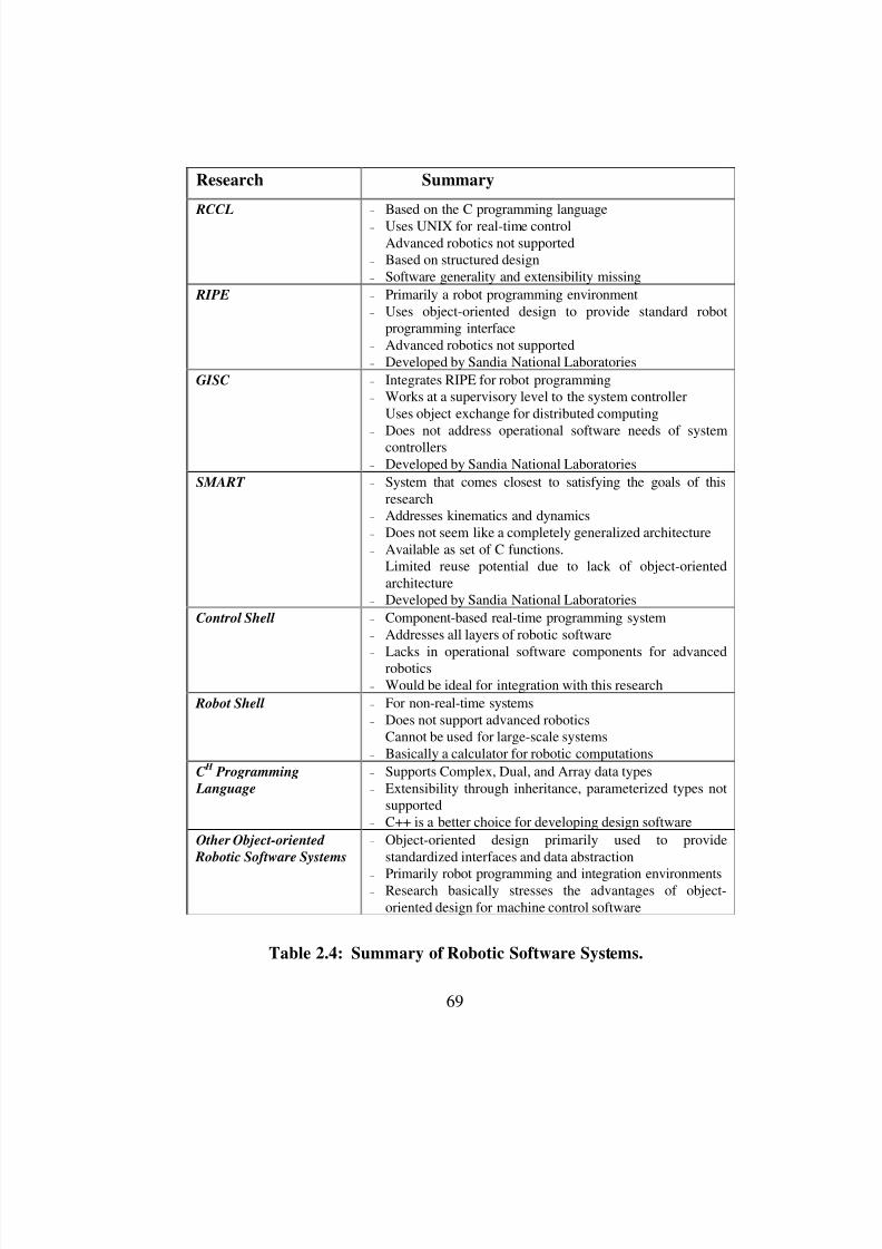
8/3/2019 Chetan Kapoor Dissertation
http://slidepdf.com/reader/full/chetan-kapoor-dissertation 93/612
69
Research Summary
RCCL − Based on the C programming language− Uses UNIX for real-time control− Advanced robotics not supported− Based on structured design− Software generality and extensibility missing
RIPE − Primarily a robot programming environment− Uses object-oriented design to provide standard robot
programming interface− Advanced robotics not supported− Developed by Sandia National Laboratories
GISC − Integrates RIPE for robot programming− Works at a supervisory level to the system controller− Uses object exchange for distributed computing−
Does not address operational software needs of systemcontrollers− Developed by Sandia National Laboratories
SMART − System that comes closest to satisfying the goals of thisresearch
− Addresses kinematics and dynamics− Does not seem like a completely generalized architecture− Available as set of C functions.− Limited reuse potential due to lack of object-oriented
architecture− Developed by Sandia National Laboratories
Control Shell − Component-based real-time programming system− Addresses all layers of robotic software
−
Lacks in operational software components for advancedrobotics− Would be ideal for integration with this research
Robot Shell − For non-real-time systems− Does not support advanced robotics− Cannot be used for large-scale systems− Basically a calculator for robotic computations
C H
Programming
Language
− Supports Complex, Dual, and Array data types− Extensibility through inheritance, parameterized types not
supported− C++ is a better choice for developing design software
Other Object-oriented
Robotic Software Systems
− Object-oriented design primarily used to providestandardized interfaces and data abstraction
− Primarily robot programming and integration environments− Research basically stresses the advantages of object-
oriented design for machine control software
Table 2.4: Summary of Robotic Software Systems.

8/3/2019 Chetan Kapoor Dissertation
http://slidepdf.com/reader/full/chetan-kapoor-dissertation 94/612
70
2.6.3. Real-time Layer
The real-time layer is the lowest layer of robotic software at the systemlevel. This layer is responsible for sending the position, velocity, or acceleration
commands to the actuators, handle external and internal events in real-time,
interface with external hardware devices and also interface with the operational
software layer. As this layer handles a number of concurrent tasks, a parallel
execution environment is best suited for this layer. Also, it is preferable to use a
real-time operating system for this layer as the desired latency to handle an event
may be very small (less than one millisecond). As this layer is based on parallel
software execution, different inter-process communication schemes can be used
for communication between concurrent tasks. The two predominant schemes are
message passing and shared memory [Silberschatz and Gahin, 1994]. Generally,
the selected scheme is dependent on the operating system being used. Work done
in this area by Rubin [1993] led to the use of the black-board (based on shared
memory) scheme as a means of software organization.
Stewart et al. [1991] also proposed and implemented a framework for
integration of real-time software modules for reconfigurable systems. This effort
was aimed at the lower level control software and provided an efficient technique
for sensor integration. This effort used structured design and was built on the
CHIMERA real-time operating system.
As mentioned above, the real-time layer interfaces with external hardware
and the actuator controllers. These actuator controllers are embedded within the
actuator casing. For an advanced actuator, these controllers will have to support
software for multiple sensors, sensor-data reduction, communications, fault-
tolerance, system-modeling, motion control, etc. Tesar [1996] outlines some of
the details regarding the design of advanced actuator systems.
8/3/2019 Chetan Kapoor Dissertation
http://slidepdf.com/reader/full/chetan-kapoor-dissertation 95/612
71
2.7. Impact of Advancement in Computer Technology
Computer technology has seen unprecedented growth in the past few
years. This has resulted in the availability of 400 MFLOP performance from
desk-side uniprocessor computers. This performance level, only a few years ago,
was the sole domain of super-computers [Hernandez et al., 1989]. Hernandez et
al.’s [1989] report on computational requirements for advanced robots predicted
0.6 MFLOP performance from personal computers in the year 1995. This
currently (1996) is around the 15 MFLOP level (Intel 100 MHz Pentium) and is
expected to reach 800 MIPS by the year 2000 [Lewis, 1994]. Also, theperformance ratio of the super-computer versus the personal computer was fixed
at 105 [Hernandez et al., 1989]. However, it is noted that this ratio is decreasing
[Lewis, 1994]. Thus, it is seen that the computer performance has increased at an
unprecedented rate belying all predictions. This increase in processor speed has
impacted current software design and programming methodologies, with object-
oriented programming gaining wide acceptance.
Robotics, though a key area that could benefit from the increase in
processor performance, has not seen a similar revolution. It is evident from the
literature, that a major part of robotics research involves developing or modifying
existing techniques for kinematics, dynamics, etc., for computational efficiency
[Izaguirre et al., 1992]. This usually destroys the generality of the software, and
also renders it in-extensible. Robotics research has also focused on designing
new computer architectures that are more suitable for computing mathematical
formulations that are pertinent to robotics [Anderson and Smiarowski,
1991][Butner et al., 1988]. Notable is the effort by Wander [1987] in which an
array processor based on a pipelined architecture was used for real-time
computation of dynamics and deflection modeling. This research showed that it

8/3/2019 Chetan Kapoor Dissertation
http://slidepdf.com/reader/full/chetan-kapoor-dissertation 96/612
72
is important to use special purpose hardware to demonstrate concepts: those that
could be implemented on generic computer hardware in the future.
The problem with robotics research in the area of designing fast computer
architectures and modifying existing algorithms for computational efficiency is
that the effort is being spent on a problem that will no longer exist in the future.
This would be due to the advancement in computer technology. An example to
illustrate this issue is presented: Wander in 1987 was able to compute robot
dynamics for a six DOF arm on a specialized and expensive array processor in 5
milliseconds using a laboriously written code. The same performance is now
(1996) possible on a low-cost high-end personal computer using generic software
environments. Nevertheless, Wander’s [1987] research showed what is possible
in the domain of real-time computing. It was not an effort in designing new
computer hardware. Furthermore, Wander’s research validated the research being
pursued at the Robotics Research Group and provided an argument for furthering
this research.
In summary, robotics research needs to progress into new areas, no matter
how computationally complex these are. Also, the research that has been done in
the area of advanced robotics has to be implemented in a generalized and object-
oriented framework that supports portability, reuse, and extensibility. Such a
framework can grow as research progresses, and it in itself could be instrumental
in spurring robotics research.
2.8. Desired Characteristics of the Software System
The historical perspective presented in the previous sections concentrated
on the evolution and development of mechanical hardware, computer hardware,
and software technologies associated with robotics. The discussion noted that a
major part of the robotic system is software. Robotic software was presented as

8/3/2019 Chetan Kapoor Dissertation
http://slidepdf.com/reader/full/chetan-kapoor-dissertation 97/612
73
consisting of three layers: the middle layer (operational software) involved
kinematics, dynamics, deflection modeling, decision making, and fault-tolerance;
the upper layer involved the robot programming environment; and the lower layer
involved the real-time control layer. From the literature review it was noted that a
considerable amount of work has been done in the development of robot
programming and low-level robot control software. All of the systems reviewed
in the literature had a rudimentary operational software layer. Additionally, it was
seen that object-oriented design was gaining popularity as a software design
technique for intelligent machine software. It was also seen that one area of
robotic software that needed further development was the operational software
layer. That is, the layer that implements the fundamental mathematical constructs
associated with high performance robot arms. A complete software architecture
for this layer needs to developed. This architecture should support software reuse,
which can be achieved via generality and extensibility.
Figure 2.13 depicts the structure of the two lower layers of robotic
software. These are, the operational software and the real-time control layer. The
figure depicts the generalized nature of the operational software components
which support kinematics, dynamics, deflection modeling, and performance
criteria. The output of these components can be channeled to a simulation or to
any physical robot through a real-time control layer.

8/3/2019 Chetan Kapoor Dissertation
http://slidepdf.com/reader/full/chetan-kapoor-dissertation 98/612
74
D namics
ForcesTorquesInertia
Criteria Compliance
W
Operational Software
Components
To Simulation
Kinematics
Real-Time Control
Components
Performance
Actuator Control
Resource
AllocationOperator Priority Setting
Figure 2.13: Desired Functionality of the Operational Software Layer.
Thus, what is needed is a reusable operational software architecture which
is built on a framework of generalized kinematics, dynamics, deflection modeling,
performance criteria and criteria fusion. This architecture should be equally
applicable to real-time control and simulation. The architecture should be

8/3/2019 Chetan Kapoor Dissertation
http://slidepdf.com/reader/full/chetan-kapoor-dissertation 99/612
75
composed of high-level software components with standardized interfaces and an
abstracted functionality. These components should be general enough to apply to
any serial robots and also should support reuse via extensibility. This software
architecture should decrease robot control program development time by 50% as
compared to robotic software systems that are currently in use. Additionally, the
development of the architecture should include the selection of the development
and execution environment, the simulation environment, the software design
methodology, the programming language and the physical robotic hardware for
testing the software.
2.9. Generalized Kinematics
Closed-form inverse kinematics can be used for computing the inverse
solution for a fully constrained robot. Fully constrained robots are those whose
number of joints is equal to the number of constraints at the end-effector. For
example, a six-jointed spatial robot is fully constrained as its number of joints is
equal to the number of independent directions the end-effector can move in (three
translations and three rotations).
Redundant robots have more joints than the number of constraints at the
end-effector. As such, the inverse kinematics solution for redundant arms leads to
an infinite number of solutions (as the system is mathematically non-square).
Numerical solutions are used to compute the inverse kinematics of redundant
arms.
Closed-form inverse kinematics solutions offer the advantages of
robustness and computational efficiency over numerical solutions. Numerical
solutions offer the advantages of reconfigurability and generality. Generality of
an inverse solution is an important issue for modular robots which are field
reconfigurable. Real-time reconfigurability of the inverse kinematics solution is
8/3/2019 Chetan Kapoor Dissertation
http://slidepdf.com/reader/full/chetan-kapoor-dissertation 100/612
76
of importance when there is a possibility of change in the robot geometry while
the robot is operational. This change in geometry of the robot may be due to a
faulted actuator. Additionally, the actuator may fail at any position, so there can
be no pre-planned inverse kinematics solutions. For a serial robot to counteract
joint failures it has to support level III fault-tolerance. Level III fault-tolerance
imparts redundant DOF to a serial robot [Sreevijayan and Tesar, 1993]. These
redundancies are used to counteract the effects of joint failures. Under normal
operation, the same redundancies are used for criteria-based performance
maximization. Thus, a generalized inverse kinematics scheme should support
criteria-based performance maximization under normal operation and should also
be reconfigurable in real-time in the event of a fault.
Extensive work has been done in the area of generalized kinematics. The
various approaches taken by researchers are detailed by Hooper [1994]. Some of
these include the Newton-Raphson numerical method, the Predictor-Corrector
numerical method, and the resolved-rate motion control using the Jacobian
inverse. Hooper [1994] discusses the strengths and limitations of these
techniques. Based on this analysis, a generalized inverse kinematics scheme that
incorporates multiple criteria is proposed by Hooper [1994]. This scheme uses
the direct-search technique for computing the inverse position solution. This
technique de-couples the application of performance criteria from the inverse
position solution and is discussed in the following sections.
2.9.1. Direct-Search Formulation
Hooper [1994] developed a generalized inverse formulation that wasbased on using the direct-search technique. The direct-search uses local
explorations in the joint-space of the robot to search for the inverse kinematics
solution. Each time a joint-space exploration is generated, the forward position
8/3/2019 Chetan Kapoor Dissertation
http://slidepdf.com/reader/full/chetan-kapoor-dissertation 101/612
77
solution is used to see whether the exploration moves the robot hand closer to the
desired position. The process of exploration generation and checking the
closeness of the hand to the desired hand location is repeated till the desired hand
location is reached.
Hooper [1994] made enhancements to the direct-search technique to
incorporate criteria-based decision making. In this case, Hooper uses a six DOF
sub-structure of the redundant arm to satisfy the end-effector constraints. The
remaining joints are used to generate null-space options. A criteria-based
decision making scheme is then used to rank all the options. Currently, Hooper
uses a closed-form inverse solution for the six DOF sub-structure inverse. The
incorporation of the closed-form solution breaks down the generality of the
inverse. For details on Hooper’s [1994] work see Chapter Three.
This research will design a generalized inverse scheme that can offer some
of the advantages of the direct-search technique, and yet is computationally
efficient and reconfigurable in real-time for use in fault-tolerance. This can be
made possible by using a numerical solution for solving the inverse position
solution for any six joints sub-structure of a redundant arm, and using the direct-
search technique for generating null-space options using the remaining joints. By
allowing the ability to pick any six joints and also allowing the capability of
changing the set of six joints, computational efficiency, criteria-based
optimization, and generality can be achieved.
2.10. Summary
All mature industries are characterized by the presence of a component
industry. An example of this is the automobile industry that is supported by a
large base of ancillary industry. Also, the personal computer hardware industry
has a distinct component industry. Surprisingly, the component industry is barely
8/3/2019 Chetan Kapoor Dissertation
http://slidepdf.com/reader/full/chetan-kapoor-dissertation 102/612
78
present for the major U.S. industry of software. This lack of a component
industry is even more noticeable in the arena of intelligent machine software.
However, there is a growing software component industry mainly due to the
popularity of object-oriented design. Object-oriented design allows the building
of software components with standardized interfaces and reuse capability. This
reuse is achieved by generality and extensibility.
Under robotic software systems, it was seen that none of these systems
implemented all of generalized kinematics, dynamics, deflection compensation,
and decision making (see Chapter One). Moreover, object-oriented design was
only used to provide better robot programming interfaces [Miller and Lennox,
1991]. In addition, most of these systems were implemented keeping in mind the
scarcity of computer resources and limited CPU power. This constraint made
these systems excessively specific and in-extensible.
Availability of cheap computer power will be a key factor in the design of
future machines. Thus, it is necessary to research robotic software systems with
an awareness of the state-of-the-art in computing. Currently, advanced UNIX
workstations offer 400 MFLOP performance. This performance level is sufficient
to implement full dynamics, kinematics, deflection modeling, and some criteria-
based decision making [Hernandez et al, 1989]. Also, the gap between personal
computers and workstations is decreasing. It is predicted that the performance of
a personal computer will increase ten times by the year 2000. This will lead to
desk-top personal computers capable of 800 million-instructions-per-second
(MIPS) [Lewis, 1994]. Currently, this performance is offered by the most
advanced workstations and low-end super-computers. This prediction for
computer technology has a definite impact on this research. With a decrease in
the price-performance ratio of computer hardware, software will be the
commodity that will be more expensive than hardware. This will force
8/3/2019 Chetan Kapoor Dissertation
http://slidepdf.com/reader/full/chetan-kapoor-dissertation 103/612
79
researchers to develop generalized algorithms using the latest in software design
and engineering methodologies: methodologies that promote reuse and
extensibility.
Thus, what is needed is a software and hardware environment that fully
exploits the breakthroughs in computer hardware and software technology. This
environment should provide the robotics researcher with a system that is built on
a framework of generalized kinematics, dynamics, deflection modeling, criteria-
based decision making, and fault-tolerance. This system should also support a 3D
graphic modeling environment that allows for visualization and demonstration.
The software for this environment should be developed using object-oriented
methodology, thus providing a path for reuse and extensibility. This software
architecture should show improvements in ‘ease of use,’ generality, organization,
‘time to code,’ and ‘time to test’ over software systems for advanced robotics that
are currently in use. Moreover, this software should be equally applicable to real-
time control. The user should be able to divert the output of this software from a
graphical environment to an actual hardware environment with minimal effort.
8/3/2019 Chetan Kapoor Dissertation
http://slidepdf.com/reader/full/chetan-kapoor-dissertation 104/612
80
Chapter Three
3. Performance-Based Hybrid Generalized Inverse
3.1. Introduction
The goal of this chapter is to discuss the enhancements that were made in
this work to Hooper’s [1994] generalized inverse kinematics scheme. First the
basics of inverse kinematics are discussed. Then the details of the direct-search
technique are discussed. This discussion includes the modifications that were
made by Hooper [1994] to achieve a practical implementation. Based on thisdiscussion, the strengths and weaknesses of Hooper’s [1994] scheme are
analyzed. This chapter then focuses on the hybrid formulation that was developed
to overcome some of the limitations of Hooper’s [1994] scheme. This chapter
also discusses a preliminary scheme for criteria fusion and addresses its
limitations. Finally, an example application is developed using this scheme. The
key characteristics and results of this application are discussed.
3.2. Inverse Kinematics
Inverse kinematics is an age old problem that almost all living beings
solve everyday. Every time a human locates his hand, he calculates the angles of
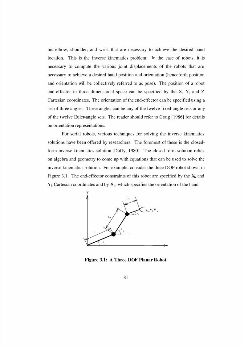
8/3/2019 Chetan Kapoor Dissertation
http://slidepdf.com/reader/full/chetan-kapoor-dissertation 105/612
81
his elbow, shoulder, and wrist that are necessary to achieve the desired hand
location. This is the inverse kinematics problem. In the case of robots, it is
necessary to compute the various joint displacements of the robots that are
necessary to achieve a desired hand position and orientation (henceforth position
and orientation will be collectively referred to as pose). The position of a robot
end-effector in three dimensional space can be specified by the X, Y, and Z
Cartesian coordinates. The orientation of the end-effector can be specified using a
set of three angles. These angles can be any of the twelve fixed-angle sets or any
of the twelve Euler-angle sets. The reader should refer to Craig [1986] for details
on orientation representations.
For serial robots, various techniques for solving the inverse kinematics
solutions have been offered by researchers. The foremost of these is the closed-
form inverse kinematics solution [Duffy, 1980]. The closed-form solution relies
on algebra and geometry to come up with equations that can be used to solve the
inverse kinematics solution. For example, consider the three DOF robot shown in
Figure 3.1. The end-effector constraints of this robot are specified by the Xh and
Yh Cartesian coordinates and by θ h, which specifies the orientation of the hand.
Y
Xh ,Yh ,θ h
θ 1
θ 2
θ 3
L1
L2
L3
Figure 3.1: A Three DOF Planar Robot.
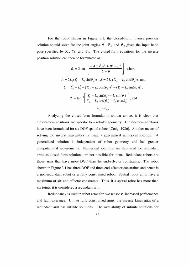
8/3/2019 Chetan Kapoor Dissertation
http://slidepdf.com/reader/full/chetan-kapoor-dissertation 106/612
82
For the robot shown in Figure 3.1, the closed-form inverse position
solution should solve for the joint angles θ 1, 2,
and3
given the input hand
pose specified by Xh, Yh, and θ h. The closed-form equations for the inverse
position solution can then be formulated as,
θ 11
2 2 2
2=− ± + −
−
−tan A A B C
C B, where
A L Y Lh h= −2 1 3( sin( )) , B L X Lh h= −2 1 3( cos( )) , and
C L L X L Y Lh h h h= − − − − −22
12
32
32( cos( )) ( sin( ))θ θ .
θ θ θ
θ θ 2
1 3 1 1
3 1 1
= − −− −
−tansin( ) sin( )
cos( ) cos( )
Y L L
X L L
h h
h h
, and
3 = h .
Analyzing the closed-form formulation shown above, it is clear that
closed-form solutions are specific to a robot’s geometry. Closed-form solutions
have been formulated for six DOF spatial robots [Craig, 1986]. Another means of
solving the inverse kinematics is using a generalized numerical solution. A
generalized solution is independent of robot geometry and has greater
computational requirements. Numerical solutions are also used for redundant
arms as closed-form solutions are not possible for them. Redundant robots are
those arms that have more DOF than the end-effector constraints. The robot
shown in Figure 3.1 has three DOF and three end-effector constraints and hence is
a non-redundant robot or a fully constrained robot. Spatial robot arms have a
maximum of six end-effector constraints. Thus, if a spatial robot has more than
six joints, it is considered a redundant arm.
Redundancy is used in robot arms for two reasons: increased performance
and fault-tolerance. Unlike fully constrained arms, the inverse kinematics of a
redundant arm has infinite solutions. The availability of infinite solutions for
8/3/2019 Chetan Kapoor Dissertation
http://slidepdf.com/reader/full/chetan-kapoor-dissertation 107/612
83
redundant arms can now be used for performance maximization. Thus, from a
given set of solutions (that satisfy the same end-effector constraints), one solution
can be selected that best satisfies some input criteria. Additionally, more than one
input criteria may be present. In this case, intelligent decision making has to be
performed for criteria fusion and normalization.
The other advantage of redundancy is fault-tolerance. Level III fault-
tolerance has been defined by Sreevijayan and Tesar [1993] as the availability of
redundant joints in a serial robot arm. Such robots can use their redundancy to
counteract joint failures. For example, if a ten DOF (four redundant joints) spatial
arm has a joint failure, it still can operate using nine DOF.
Thus, what is needed is an inverse kinematics scheme that applies to
redundant robots and actively uses redundancy in the mechanical structure. This
scheme should be general enough to apply to all possible robot geometries.
Additionally, under normal operation this scheme should maximize performance
based on input criteria and in the event of a fault should use the redundancy to
counteract the fault. To support fault-tolerance, the scheme should be
reconfigurable in real-time without human intervention.
Various generalized inverse kinematics schemes have been proposed by
researchers. One of these is the direct-search technique proposed by Hooper
[1994]. This scheme allows for efficient incorporation of multiple criteria and
supports Level III fault-tolerance. The following section discusses this scheme in
more detail.
3.3. Direct Search TechniqueHooper’s [1994] scheme uses a direct-search approach that is based on
using the forward position solution to search for a suitable inverse position
solution. This technique is then extended to redundant robots and the inclusion of
8/3/2019 Chetan Kapoor Dissertation
http://slidepdf.com/reader/full/chetan-kapoor-dissertation 108/612
84
multiple criteria. In the most basic sense, direct-search is a numerical method for
solving equations by using a set of trial solutions to guide the search. The search
is direct because it does not explicitly evaluate derivatives as do gradient and
high-order numerical methods. The direct-search technique begins by an estimate
of a solution, which serves as a base point. From this base point, local
explorations are made. From amongst the local explorations, a new base point is
picked which reduces the error in the solution. This process continues until the
search, at least a successful one, finds a solution. [Hooper, 1994]
The direct-search technique when applied to serial robots involves using
the forward position solution to guide the search. The input into the direct-search
formulation is a desired hand location of the end-effector. The output from the
direct-search is the joint angle solution that will achieve the desired hand location.
The steps for solving the inverse kinematics solution are as follows:
1) Pick a starting joint angle configuration of the robot. This will be the base
point of the search.
2) The next step is to perform a local exploration around the base point. The
idea here is to generate enough options. That is to generate a set of joint angle
configurations. This is done by simulating perturbations in the joints of the
robot. Mathematically, perturbing the joint displacements a small amount,
∆ , from their current values, θ , generates a set of local configuration
options:
θ θ θ θ ∧ ∧
= + ∈: ∆ 3.1
where ∈ is an arbitrary sweep vector with all elements equal to ± 1 or 0. The
vector of current displacement values, , is the base point for perturbations.
At the base point, ∈= 0 . All other ∈ with elements equal to combinations of
± 1 and 0 generate other options. Based on the selection of ∈, a different
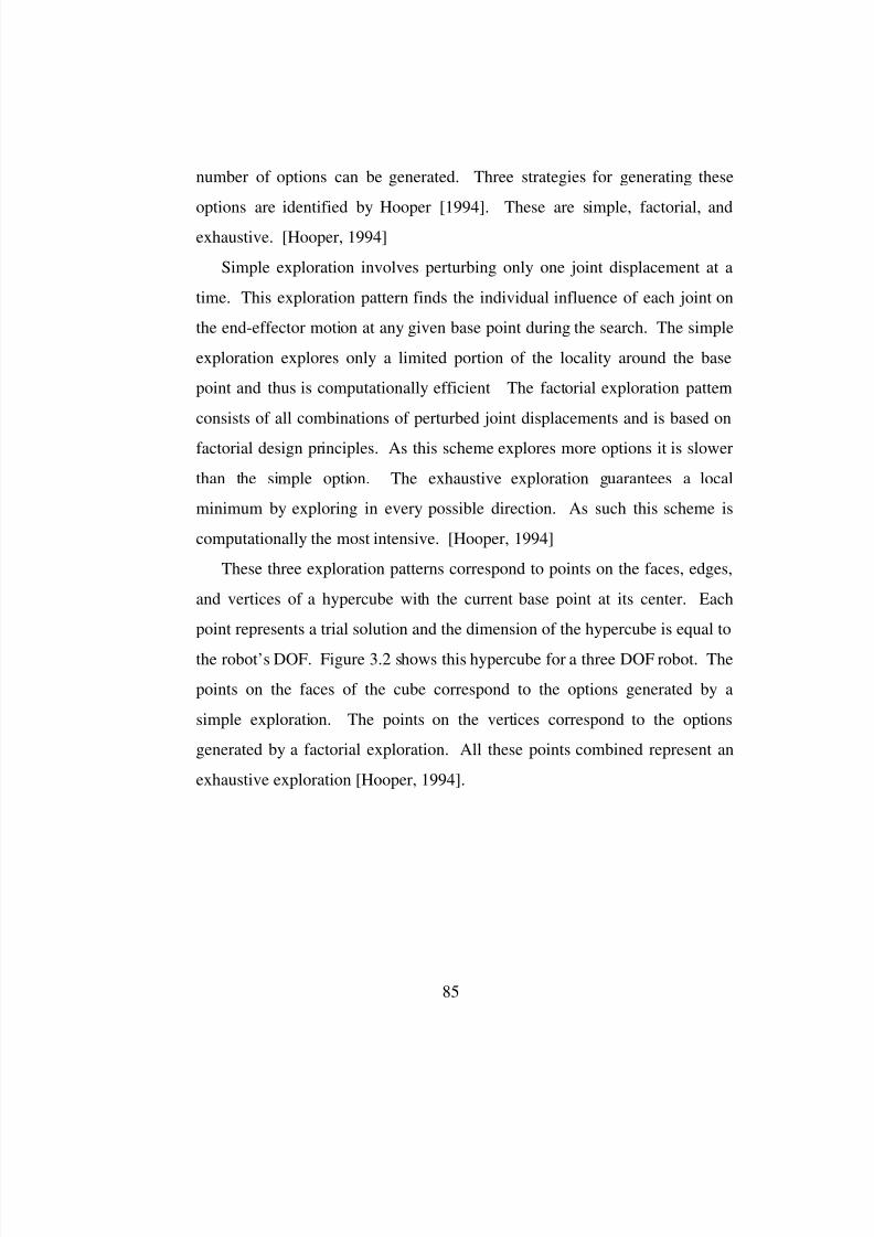
8/3/2019 Chetan Kapoor Dissertation
http://slidepdf.com/reader/full/chetan-kapoor-dissertation 109/612
85
number of options can be generated. Three strategies for generating these
options are identified by Hooper [1994]. These are simple, factorial, and
exhaustive. [Hooper, 1994]
Simple exploration involves perturbing only one joint displacement at a
time. This exploration pattern finds the individual influence of each joint on
the end-effector motion at any given base point during the search. The simple
exploration explores only a limited portion of the locality around the base
point and thus is computationally efficient The factorial exploration pattern
consists of all combinations of perturbed joint displacements and is based on
factorial design principles. As this scheme explores more options it is slower
than the simple option. The exhaustive exploration guarantees a local
minimum by exploring in every possible direction. As such this scheme is
computationally the most intensive. [Hooper, 1994]
These three exploration patterns correspond to points on the faces, edges,
and vertices of a hypercube with the current base point at its center. Each
point represents a trial solution and the dimension of the hypercube is equal to
the robot’s DOF. Figure 3.2 shows this hypercube for a three DOF robot. The
points on the faces of the cube correspond to the options generated by a
simple exploration. The points on the vertices correspond to the options
generated by a factorial exploration. All these points combined represent an
exhaustive exploration [Hooper, 1994].
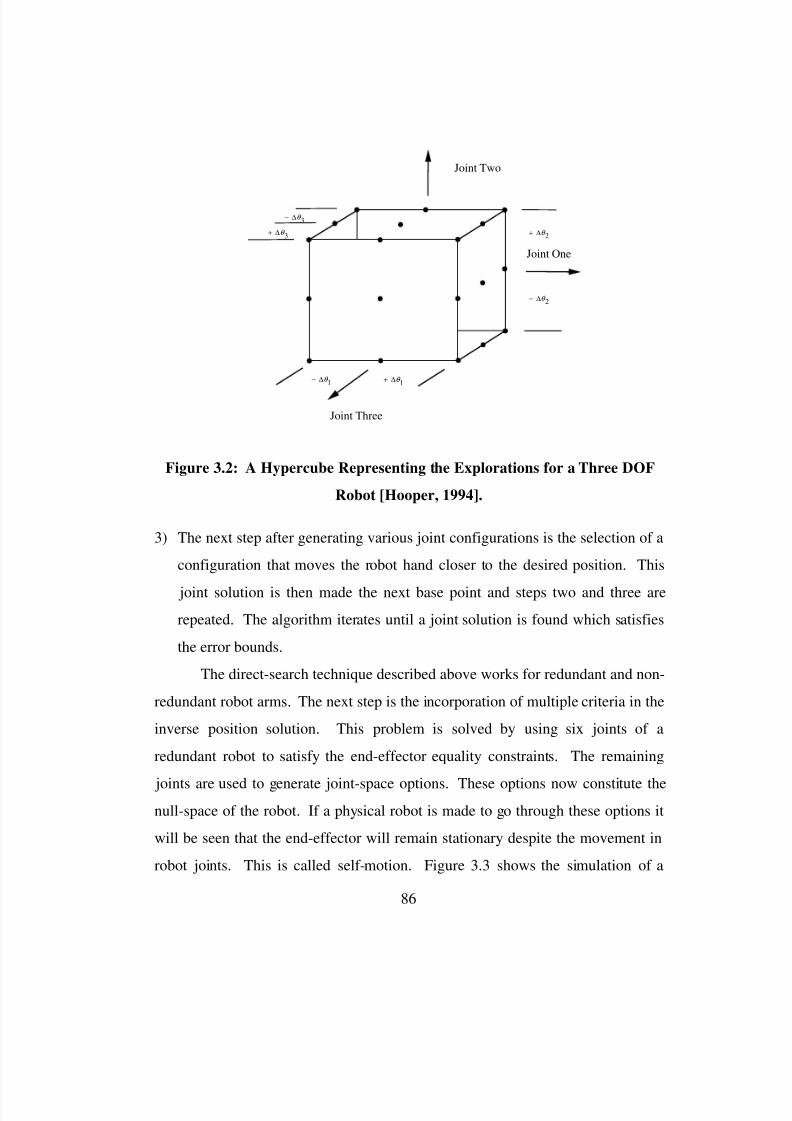
8/3/2019 Chetan Kapoor Dissertation
http://slidepdf.com/reader/full/chetan-kapoor-dissertation 110/612
86
3) The next step after generating various joint configurations is the selection of a
configuration that moves the robot hand closer to the desired position. This
joint solution is then made the next base point and steps two and three are
repeated. The algorithm iterates until a joint solution is found which satisfies
the error bounds.
The direct-search technique described above works for redundant and non-
redundant robot arms. The next step is the incorporation of multiple criteria in the
inverse position solution. This problem is solved by using six joints of a
redundant robot to satisfy the end-effector equality constraints. The remaining
joints are used to generate joint-space options. These options now constitute the
null-space of the robot. If a physical robot is made to go through these options it
will be seen that the end-effector will remain stationary despite the movement in
robot joints. This is called self-motion. Figure 3.3 shows the simulation of a
+ ∆θ 3
− ∆θ 3
Joint One
Joint Two
Joint Three
+ ∆θ 1− ∆θ 1
− ∆θ 2
+ ∆θ 2
Figure 3.2: A Hypercube Representing the Explorations for a Three DOF
Robot [Hooper, 1994].
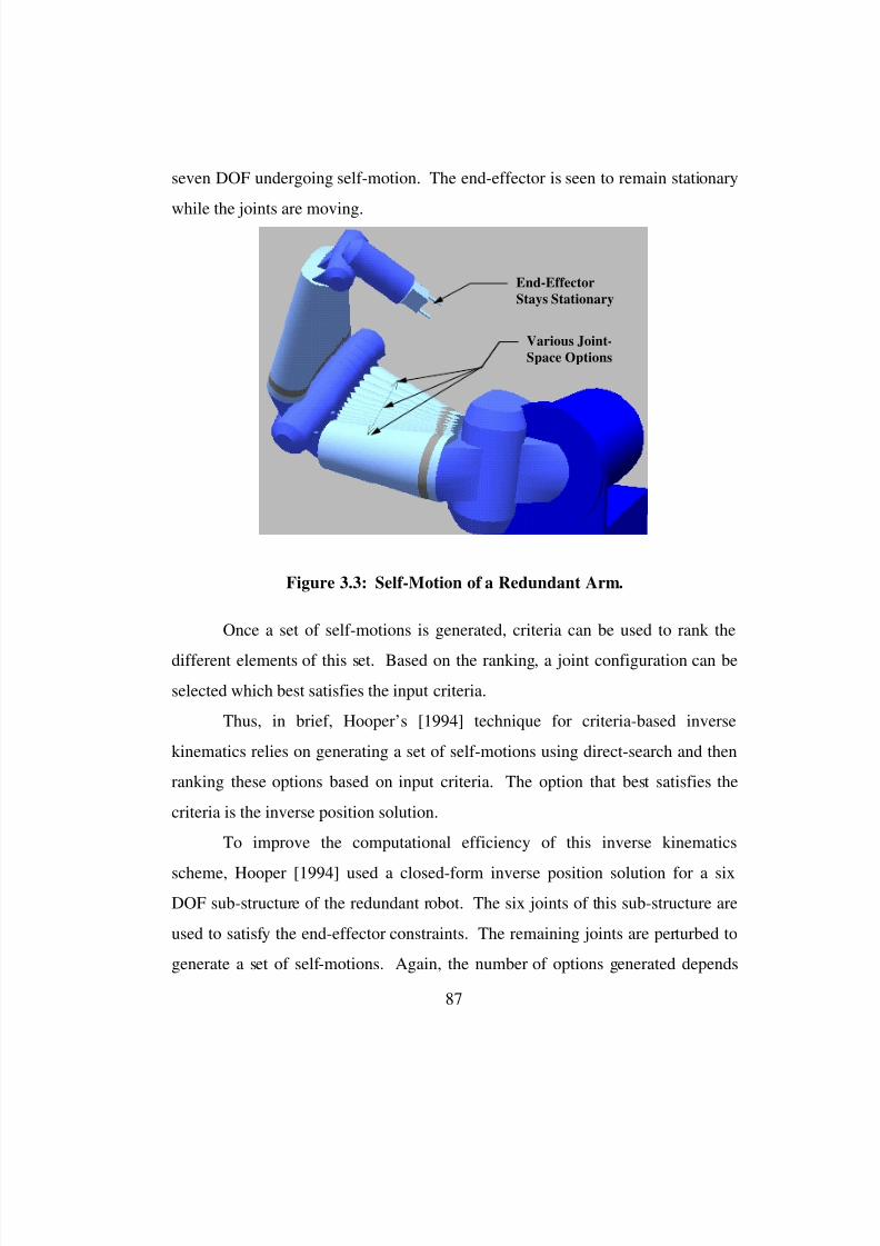
8/3/2019 Chetan Kapoor Dissertation
http://slidepdf.com/reader/full/chetan-kapoor-dissertation 111/612
87
seven DOF undergoing self-motion. The end-effector is seen to remain stationary
while the joints are moving.
Once a set of self-motions is generated, criteria can be used to rank the
different elements of this set. Based on the ranking, a joint configuration can be
selected which best satisfies the input criteria.
Thus, in brief, Hooper’s [1994] technique for criteria-based inverse
kinematics relies on generating a set of self-motions using direct-search and then
ranking these options based on input criteria. The option that best satisfies the
criteria is the inverse position solution.
To improve the computational efficiency of this inverse kinematics
scheme, Hooper [1994] used a closed-form inverse position solution for a six
DOF sub-structure of the redundant robot. The six joints of this sub-structure are
used to satisfy the end-effector constraints. The remaining joints are perturbed to
generate a set of self-motions. Again, the number of options generated depends
End-Effector
Stays Stationary
Various Joint-
Space Options
Figure 3.3: Self-Motion of a Redundant Arm.
8/3/2019 Chetan Kapoor Dissertation
http://slidepdf.com/reader/full/chetan-kapoor-dissertation 112/612
88
upon the type of search (simple, factorial, exhaustive). The generated options are
then ranked based on the input criteria. For example, for a seven DOF robot, a set
of six joints are picked that have a closed-form inverse position solution. The
closed-form solution is then formulated for these six joints and for the remaining
seventh joint, simulated perturbations are used to generate options. Figure 3.4
illustrates the direct-search technique that incorporates a closed-form inverse
solution and decision making. The next two sections discuss the strengths and
weaknesses of this technique.
Input Hand Position
Performance Criteria
(Rank all options based onmultiple input criteria)
Inverse Solution
(Choose best option)
Generate Options
Closed-form 6-DOF
Inverse Position Solution
(Satisfies End-EffectorConstraints)
Direct-Search on Free Joints
(Explorations: Simple, Factorial,or Exhaustive)
Figure 3.4: Inverse Kinematics Using Direct-Search and a Closed-Form
Inverse Position Solution.
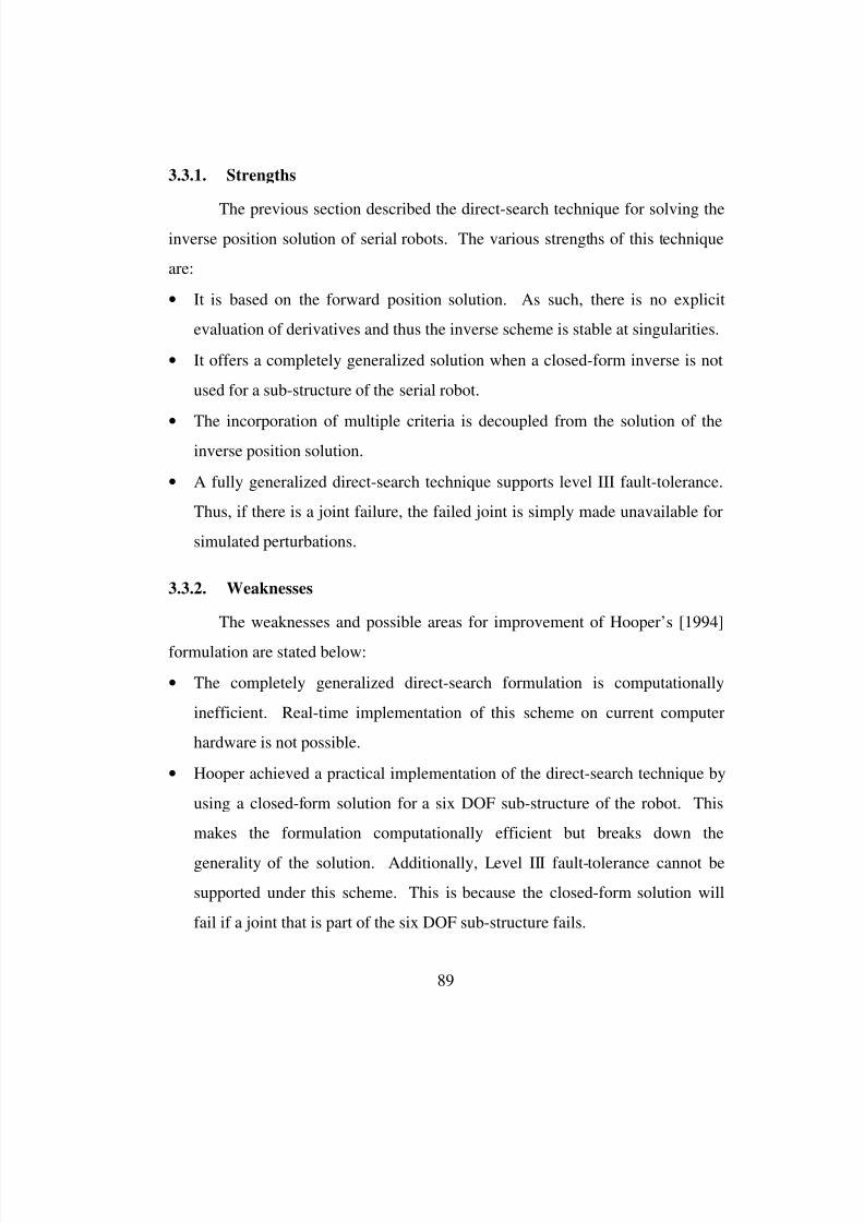
8/3/2019 Chetan Kapoor Dissertation
http://slidepdf.com/reader/full/chetan-kapoor-dissertation 113/612
89
3.3.1. Strengths
The previous section described the direct-search technique for solving theinverse position solution of serial robots. The various strengths of this technique
are:
• It is based on the forward position solution. As such, there is no explicit
evaluation of derivatives and thus the inverse scheme is stable at singularities.
• It offers a completely generalized solution when a closed-form inverse is not
used for a sub-structure of the serial robot.
•
The incorporation of multiple criteria is decoupled from the solution of theinverse position solution.
• A fully generalized direct-search technique supports level III fault-tolerance.
Thus, if there is a joint failure, the failed joint is simply made unavailable for
simulated perturbations.
3.3.2. Weaknesses
The weaknesses and possible areas for improvement of Hooper’s [1994]
formulation are stated below:
• The completely generalized direct-search formulation is computationally
inefficient. Real-time implementation of this scheme on current computer
hardware is not possible.
• Hooper achieved a practical implementation of the direct-search technique by
using a closed-form solution for a six DOF sub-structure of the robot. This
makes the formulation computationally efficient but breaks down the
generality of the solution. Additionally, Level III fault-tolerance cannot be
supported under this scheme. This is because the closed-form solution will
fail if a joint that is part of the six DOF sub-structure fails.

8/3/2019 Chetan Kapoor Dissertation
http://slidepdf.com/reader/full/chetan-kapoor-dissertation 114/612
90
As an extension to Hooper’s [1994] work, a generalized inverse scheme
needs to be designed that can offer some of the advantages of the direct-search
technique, and yet is computationally efficient and reconfigurable in real-time for
use in fault-tolerance. This can be made possible by using a numerical solution
for solving for any six joints of a redundant arm, and using the direct-search
technique for the remaining joints. By allowing the ability to pick any six joints
and allowing the capability of changing the set of six joints, computational
efficiency, criteria-based optimization, and generality can be achieved.
3.4. Hybrid Formulation
As mentioned earlier, Hooper’s technique of using a closed-form solution
for a six DOF sub-structure of a redundant arm is not generalized and
reconfigurable. One way of overcoming this limitation is to use a generalized
inverse solution for the six DOF sub-structure. Figure 3.4 illustrated Hooper’s
scheme that used a closed-form solution. The hybrid scheme that uses a
generalized six DOF inverse, supports multicriteria decision-making and fault-
tolerance, is shown in Figure 3.5.
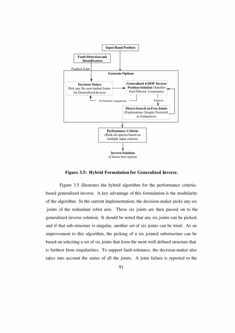
8/3/2019 Chetan Kapoor Dissertation
http://slidepdf.com/reader/full/chetan-kapoor-dissertation 115/612
91
Figure 3.5 illustrates the hybrid algorithm for the performance criteria-
based generalized inverse. A key advantage of this formulation is the modularity
of the algorithm. In the current implementation, the decision-maker picks any six
joints of the redundant robot arm. These six joints are then passed on to the
generalized inverse solution. It should be noted that any six joints can be picked,
and if that sub-structure is singular, another set of six joints can be tried. As an
improvement to this algorithm, the picking of a six jointed substructure can be
based on selecting a set of six joints that form the most well defined structure that
is furthest from singularities. To support fault-tolerance, the decision-maker also
takes into account the status of all the joints. A joint failure is reported to the
No Solution (singularity)
Input Hand Position
Performance Criteria
(Rank all options based onmultiple input criteria)
Inverse Solution
(Choose best option)
Generate Options
Fault-Detection andIdentification
Faulted-Joint
Solution
Generalized 6-DOF Inverse
Position Solution (SatisfiesEnd-Effector Constraints)
Decision-Maker
Pick any Six non-faulted Jointsfor Generalized Inverse
Direct-Search on Free Joints
(Explorations: Simple, Factorial,
or Exhaustive)
Figure 3.5: Hybrid Formulation for Generalized Inverse.

8/3/2019 Chetan Kapoor Dissertation
http://slidepdf.com/reader/full/chetan-kapoor-dissertation 116/612
92
decision-maker by the fault detection and identification sub-system. Once a joint
has failed, it is rendered unfit for use in the generalized inverse and for option
generation by direct-search.
The generalized inverse solution receives a set of six joints from the
decision-maker. The generalized inverse then uses these six joints to satisfy the
end-effector constraints. If in the process a singularity is encountered, the
decision-maker is informed and another set of six joints is picked and the process
repeated. After the end-effector constraints are satisfied, the direct-search sub-
system is informed. This sub-system then generates various joint angle options
that all satisfy the desired input hand location. The option generation may take
place using any of the three exploration patterns that were mentioned earlier. It
should be noted that the option generation takes place in a loop with the
generalized inverse. Every time a joint is perturbed, the geometry of the six DOF
sub-structure in use by the generalized inverse changes. In essence, the generate
options sub-system generates a set of self-motions of the robot arm around the
base point. This set of self-motions (or joint-space options) is then passed onto
the performance criteria sub-system. The performance criteria sub-system ranks
these options based on the criteria. The highest ranking option is then chosen as
the solution.
3.4.1. Generalized Inverse Scheme
As mentioned earlier, the hybrid scheme uses a generalized inverse for a
six DOF sub-structure of the robot. Thus, it was a key part of this research to
select and develop a generalized inverse scheme that could be used for thispurpose. The set of requirements for the generalized inverse should include:
• computational efficiency,
• applicability to any six jointed sub-structure of the robot,

8/3/2019 Chetan Kapoor Dissertation
http://slidepdf.com/reader/full/chetan-kapoor-dissertation 117/612
93
• robustness, and
•
prevalence and proven use in the research community.The resolved rate motion control inverse kinematics scheme proposed by
Whitney was analyzed for this purpose [Whitney, 1969]. This scheme is velocity-
based and uses the Jacobian matrix to solve the inverse kinematics solution.
Additionally, this scheme satisfies the requirements of computational efficiency,
and reconfigurability. This scheme is widely used in the research community and
various extensions have been developed to make it robust around singularities
[Nakamura, 1991]. The following paragraphs explain the resolved rate
formulation in detail and also discuss how the scheme is used to compute the
inverse solution for a sub-structure of a serial robot.
The forward position solution for a serial robot involves calculating the
end-effector position and orientation based on the joint position of the arm. This
is mathematically represented as:
x = f(q) 3.2
where x is the hand position and orientation of the robot and q is the vector of
joint displacements. The inverse position solution involves computing the joint
angle solution for a given hand position. This can be represented as:
q = f (x)−1
3.3
In general, the above formulation is non-linear and there are no analytical
closed-form solutions for a general robot structure. To solve this problem,
differential kinematics based on resolved rate motion control was introduced by
Whitney [1969]. This involves computing the joint velocities based on given end-
effector velocities. This is represented as:
x J q.
=.
3.4
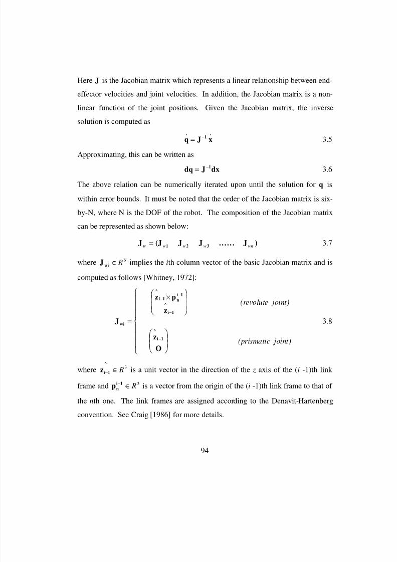
8/3/2019 Chetan Kapoor Dissertation
http://slidepdf.com/reader/full/chetan-kapoor-dissertation 118/612
94
Here J is the Jacobian matrix which represents a linear relationship between end-
effector velocities and joint velocities. In addition, the Jacobian matrix is a non-
linear function of the joint positions. Given the Jacobian matrix, the inverse
solution is computed as
q J x.
1.
= − 3.5
Approximating, this can be written as
dq J dx1= − 3.6
The above relation can be numerically iterated upon until the solution for q is
within error bounds. It must be noted that the order of the Jacobian matrix is six-
by-N, where N is the DOF of the robot. The composition of the Jacobian matrix
can be represented as shown below:
J (J J J .. . . . . J )1 2 3w w w w wn= 3.7
where Jwi ∈ R6 implies the ith column vector of the basic Jacobian matrix and is
computed as follows [Whitney, 1972]:
J
z p
z
z
O
wi
^
i 1 ni 1
^
i 1
^
i 1
=
×
− −
−
−
(revolute joint)
(prismatic joint)
3.8
where zi 1
^
− ∈ R3 is a unit vector in the direction of the z axis of the (i -1)th link
frame and pn
i 1− ∈ R3 is a vector from the origin of the (i -1)th link frame to that of
the nth one. The link frames are assigned according to the Denavit-Hartenberg
convention. See Craig [1986] for more details.

8/3/2019 Chetan Kapoor Dissertation
http://slidepdf.com/reader/full/chetan-kapoor-dissertation 119/612
95
As mentioned before, the hybrid scheme uses a numerical technique
instead of a closed-form technique to compute the inverse position solution for
the six joint substructure of the robot. This is done by computing the Jacobian
matrix for the six joints that comprise the substructure. Thus, in this scheme the
Jacobian is always of order six-by-six. Based on this Jacobian, the inverse
position solution is calculated by numerical iteration over Equation 3.6. For
example, consider an eight DOF robot for which the inverse position solution is
solved using the hybrid technique. As the robot in question has two redundant
joints, these joints will be used for simulated perturbations. The remaining joints
will be used to satisfy the end-effector constraints using the resolved rate motion
control technique. The algorithm for this can begin with selecting the last six
joints of the redundant arm to comprise the six DOF sub-structure. The Jacobian
is now only computed for the last six joints. The first two joints are
systematically perturbed to generate the joint-space options.
Restricting the Jacobian size to a six-by-six has the advantages of
computational efficiency and the ability to use optimized routines for solving
linear equations. In this scheme, the selection of six joints is controlled by a
decision maker. If there is a joint failure the joint is made unavailable for use by
the numerical solution. Also, if the Jacobian matrix for the selected six joints is
ill-conditioned (condition number through Gaussian elimination), the decision
maker selects another set of six joints. In addition, a singular value
decomposition of the Jacobian matrix can be used to get desired constraint
equations that can aid in the selection of an ideal six joint sub-structure that has
the best condition number.
8/3/2019 Chetan Kapoor Dissertation
http://slidepdf.com/reader/full/chetan-kapoor-dissertation 120/612
96
3.4.2. Options Ranking
The output of the option generation part of the hybrid algorithm is a set of joint angle solutions that satisfy the desired end-effector constraints. The next
step is the effective ranking of these options based on input criteria. The
University of Texas Robotics Research Group has put forth a concerted and
systematic effort in developing a set of performance criteria that are relevant to
robot operations. Cleary and Tesar [1990] arranged these criteria into the
following categories: geometric, inertial, kinetic energy distribution, and system
compliance. The geometric criteria are further subdivided into first-order (based
on the Jacobian matrix) and second-order (based on the Hessian array). These
criteria are task independent and based only on the geometry of the robot. The
inertial criteria are based on the dynamic model of forces and torque within the
robot. The kinetic energy performance criteria are based on the overall effective
inertia of the system. The compliance criterion describe the robot’s ability to
perform precision operations under load. The reader should refer to Hooper
[1994], Van Doren [1992], and Browning [1996] for a detailed explanation of the
various performance criteria.
Once a set of performance criteria is available, the next step is the
application of these criteria to the various joint-space options. This is done by
computing the criterion value for each joint-space option and then sorting the
various options based on the criterion value. Figure 3.5 illustrates this process.
The options are represented as a1 , a2 , a3 , ……an-1 , an. The performance criterion
is applied to each of these options and the corresponding criterion value is (c1 , c2 ,
c3 , ……cn-1 , cn) computed. After this, the criteria values are sorted. The end
result is a sorted list of all options.
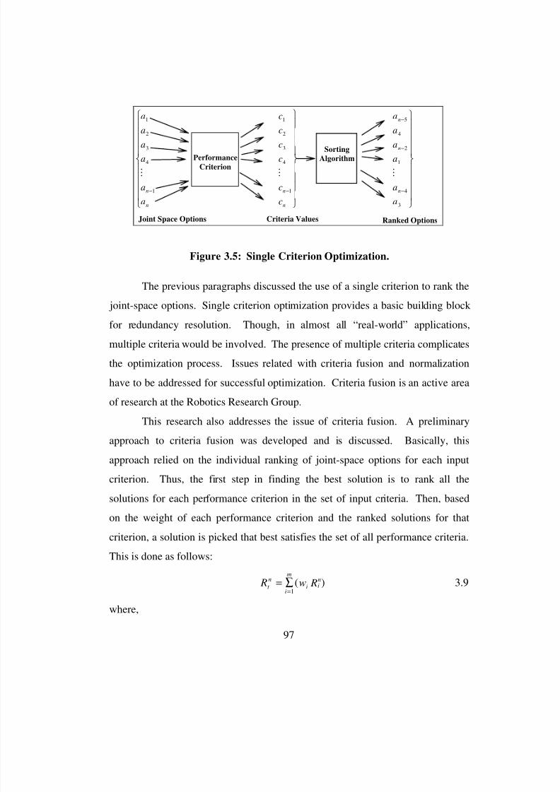
8/3/2019 Chetan Kapoor Dissertation
http://slidepdf.com/reader/full/chetan-kapoor-dissertation 121/612
97
a
a
a
a
a
a
n
n
1
2
3
4
1
M
−
c
c
c
c
c
c
n
n
1
2
3
4
1
M
−
a
a
a
a
a
a
n
n
n
−
−
−
5
4
2
1
4
3
M
Joint Space Options
Performance
Criterion
Sorting
Algorithm
Criteria Values Ranked Options
Figure 3.5: Single Criterion Optimization.
The previous paragraphs discussed the use of a single criterion to rank the
joint-space options. Single criterion optimization provides a basic building block
for redundancy resolution. Though, in almost all “real-world” applications,
multiple criteria would be involved. The presence of multiple criteria complicates
the optimization process. Issues related with criteria fusion and normalization
have to be addressed for successful optimization. Criteria fusion is an active area
of research at the Robotics Research Group.
This research also addresses the issue of criteria fusion. A preliminary
approach to criteria fusion was developed and is discussed. Basically, this
approach relied on the individual ranking of joint-space options for each input
criterion. Thus, the first step in finding the best solution is to rank all the
solutions for each performance criterion in the set of input criteria. Then, based
on the weight of each performance criterion and the ranked solutions for that
criterion, a solution is picked that best satisfies the set of all performance criteria.
This is done as follows:
R w Rt
n
i in
i
m
= ∑=
( )1
3.9
where,
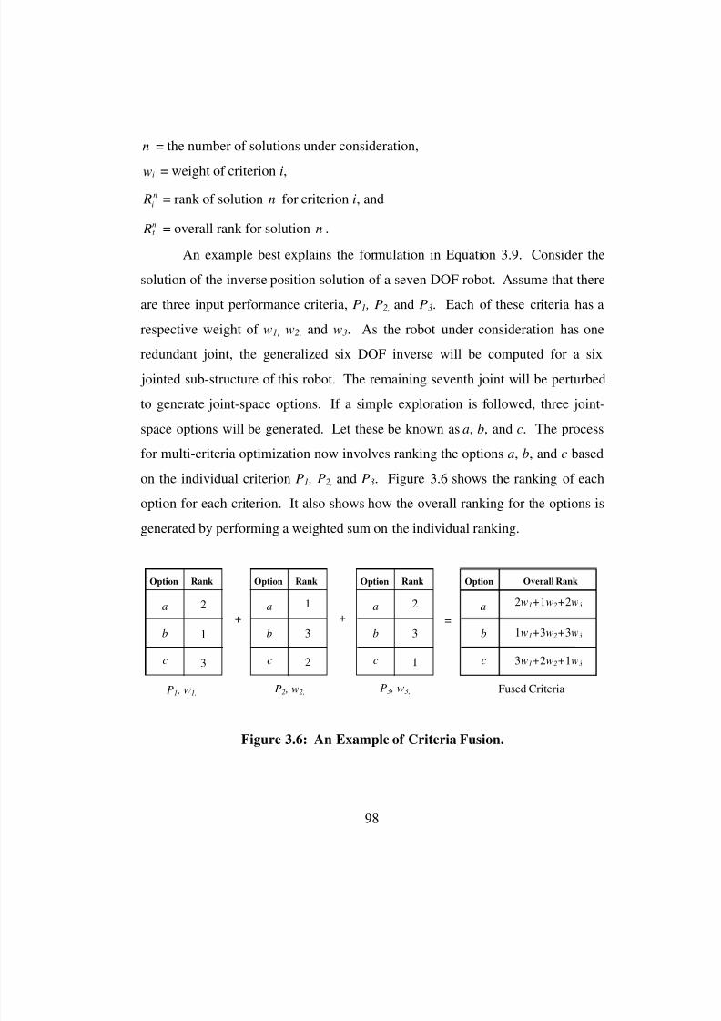
8/3/2019 Chetan Kapoor Dissertation
http://slidepdf.com/reader/full/chetan-kapoor-dissertation 122/612
98
n = the number of solutions under consideration,
iw = weight of criterion i,
Ri
n = rank of solution n for criterion i, and
t n R = overall rank for solution n .
An example best explains the formulation in Equation 3.9. Consider the
solution of the inverse position solution of a seven DOF robot. Assume that there
are three input performance criteria, P1 , P2, and P3. Each of these criteria has a
respective weight of w1, w2, and w3. As the robot under consideration has one
redundant joint, the generalized six DOF inverse will be computed for a six jointed sub-structure of this robot. The remaining seventh joint will be perturbed
to generate joint-space options. If a simple exploration is followed, three joint-
space options will be generated. Let these be known as a, b, and c. The process
for multi-criteria optimization now involves ranking the options a, b, and c based
on the individual criterion P1 , P2, and P3. Figure 3.6 shows the ranking of each
option for each criterion. It also shows how the overall ranking for the options is
generated by performing a weighted sum on the individual ranking.
Option Rank
a
b
c
Option Rank
a
b
c
Option Rank
a
b
c
Option Overall Rank
a
b
c
+ + =
P1 , w1, P2 , w2, P3 , w3, Fused Criteria
2
1
3
1
3
2
2
3
1
2w1+1w2+2w3
1w1+3w2+3w3
3w1+2w2+1w3
Figure 3.6: An Example of Criteria Fusion.
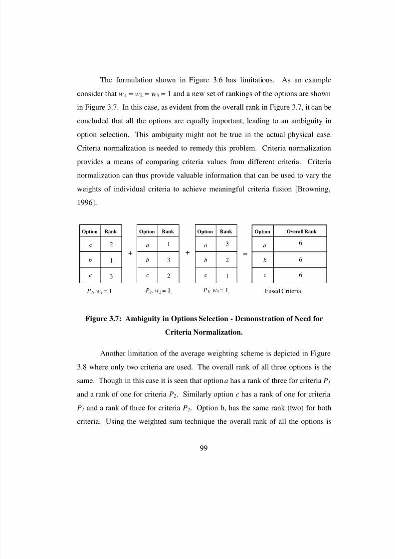
8/3/2019 Chetan Kapoor Dissertation
http://slidepdf.com/reader/full/chetan-kapoor-dissertation 123/612
99
The formulation shown in Figure 3.6 has limitations. As an example
consider that w1
= w2
= w3
= 1 and a new set of rankings of the options are shown
in Figure 3.7. In this case, as evident from the overall rank in Figure 3.7, it can be
concluded that all the options are equally important, leading to an ambiguity in
option selection. This ambiguity might not be true in the actual physical case.
Criteria normalization is needed to remedy this problem. Criteria normalization
provides a means of comparing criteria values from different criteria. Criteria
normalization can thus provide valuable information that can be used to vary the
weights of individual criteria to achieve meaningful criteria fusion [Browning,
1996].
Another limitation of the average weighting scheme is depicted in Figure
3.8 where only two criteria are used. The overall rank of all three options is the
same. Though in this case it is seen that option a has a rank of three for criteria P1
and a rank of one for criteria P2. Similarly option c has a rank of one for criteria
P1 and a rank of three for criteria P2. Option b, has the same rank (two) for both
criteria. Using the weighted sum technique the overall rank of all the options is
Option Rank
a
b
c
Option Rank
a
b
c
Option Rank
a
b
c
Option Overall Rank
a
b
c
+ + =
P1 , w1 = 1P
2 , w
2 = 1 ,P
3 , w
3= 1
, Fused Criteria
2
1
3
1
3
2
3
2
1
6
6
6
Figure 3.7: Ambiguity in Options Selection - Demonstration of Need for
Criteria Normalization.

8/3/2019 Chetan Kapoor Dissertation
http://slidepdf.com/reader/full/chetan-kapoor-dissertation 124/612
100
four. This again leads to ambiguity in the option selection process. Though it is
clear from the individual rankings that option b is the best choice. This is because
option b has the minimum variance over different criteria.
A solution can be offered to the problem shown in Figure 3.8. This
solution is applied only to the ambiguity cases demonstrated in Figures 3.7 and
3.8. The first step of this solution is to compute the variance in the rank of each
option. The option with the minimum variance is then selected as the best option.
For example, in the ambiguity case shown in Figure 3.8, it is seen that the
variance of rank is minimum for option b. Thus, option b offers the best solution.
However, it should be noted that this scheme of using variance to resolve
ambiguity breaks down for the ambiguity example shown in Figure 3.7. In that
example, the ambiguity is evident. If variance is used to resolve the ambiguity, it
is seen that all the three options have the same variance. So the ambiguity still
exists. In this case criteria normalization can be used to resolve the ambiguity.
In summary, a criteria fusion scheme is proposed that uses a weighted sum
of ranked options for each criteria to compute an overall ranking. Each criteria
has an associated weight, determined from the task at hand. Ambiguity can arise
Option Rank
a
b
c
Option Rank
a
b
c
Option Overall Rank
a
b
c
+ =
P1 , w1 = 1 P2 , w2 = 1 , Fused Criteria
3
2
1
1
2
3
4
4
4
Figure 3.8: Ambiguity in Options Selection - Need for Variance.
8/3/2019 Chetan Kapoor Dissertation
http://slidepdf.com/reader/full/chetan-kapoor-dissertation 125/612
101
when this scheme is used. This ambiguity is a result of different options getting
the same overall rank. Two steps for resolving this ambiguity have been
proposed. The first step involves computing the variance of the rank of an option
from one criteria to another. The option with the minimum variance is then
selected as the best option. When variance calculation does not resolve the issue,
criteria normalization has to be used to resolve conflicts.
3.5. Example of Hybrid Generalized Inverse
The performance-based hybrid generalized inverse scheme was
implemented using the software components developed as a part of this research.
The hybrid generalized inverse was then demonstrated on a seven DOF robot.
This robot comprised one of the arms of the seventeen DOF dual-arm robotic
manipulator from Robotics Research Corporation. The algorithm was first tested
under simulation and then tested interactively in real-time on one of the arms of
the dual-arm robot.
This demonstration involved the use of a seven DOF arm whose end-
effector was interactively controlled by a six DOF input device. The computation
of the inverse position followed the steps illustrated in Figure 3.5. These are
discussed below for this specific case:
1) Six joints of the seven DOF robot were selected to comprise the sub-structure
for which the generalized inverse was to be computed. These were joints one
and joints three through seven.
2) Joint two was selected for the application of the direct-search. Thus, this joint
was perturbed to generate options. As there is only one redundancy, only
three options are generated.
3) Three criteria were used for decision making and selection of the options.
These are discussed in the next section.
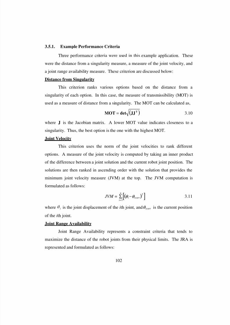
8/3/2019 Chetan Kapoor Dissertation
http://slidepdf.com/reader/full/chetan-kapoor-dissertation 126/612
102
3.5.1. Example Performance Criteria
Three performance criteria were used in this example application. Thesewere the distance from a singularity measure, a measure of the joint velocity, and
a joint range availability measure. These criterion are discussed below:
Distance from Singularity
This criterion ranks various options based on the distance from a
singularity of each option. In this case, the measure of transmissibility (MOT) is
used as a measure of distance from a singularity. The MOT can be calculated as,
( )MOT det JJT
= 3.10
where J is the Jacobian matrix. A lower MOT value indicates closeness to a
singularity. Thus, the best option is the one with the highest MOT.
Joint Velocity
This criterion uses the norm of the joint velocities to rank different
options. A measure of the joint velocity is computed by taking an inner product
of the difference between a joint solution and the current robot joint position. The
solutions are then ranked in ascending order with the solution that provides theminimum joint velocity measure (JVM) at the top. The JVM computation is
formulated as follows:
( )[ ] JVM = i icurr i=
n
θ θ −∑ 2
1
3.11
where i is the joint displacement of the ith joint, and icurr θ is the current position
of the ith joint.
Joint Range Availability
Joint Range Availability represents a constraint criteria that tends to
maximize the distance of the robot joints from their physical limits. The JRA is
represented and formulated as follows:
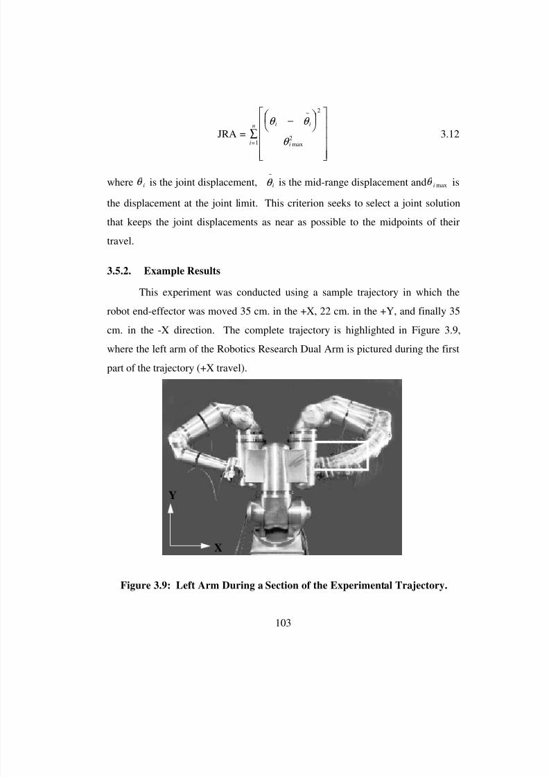
8/3/2019 Chetan Kapoor Dissertation
http://slidepdf.com/reader/full/chetan-kapoor-dissertation 127/612
103
JRA =
i i
ii=
nθ θ
θ
−
∑
~
max
2
21 3.12
where i is the joint displacement, iθ
~
is the mid-range displacement and i max is
the displacement at the joint limit. This criterion seeks to select a joint solution
that keeps the joint displacements as near as possible to the midpoints of their
travel.
3.5.2. Example Results
This experiment was conducted using a sample trajectory in which the
robot end-effector was moved 35 cm. in the +X, 22 cm. in the +Y, and finally 35
cm. in the -X direction. The complete trajectory is highlighted in Figure 3.9,
where the left arm of the Robotics Research Dual Arm is pictured during the first
part of the trajectory (+X travel).
X
Y
Figure 3.9: Left Arm During a Section of the Experimental Trajectory.
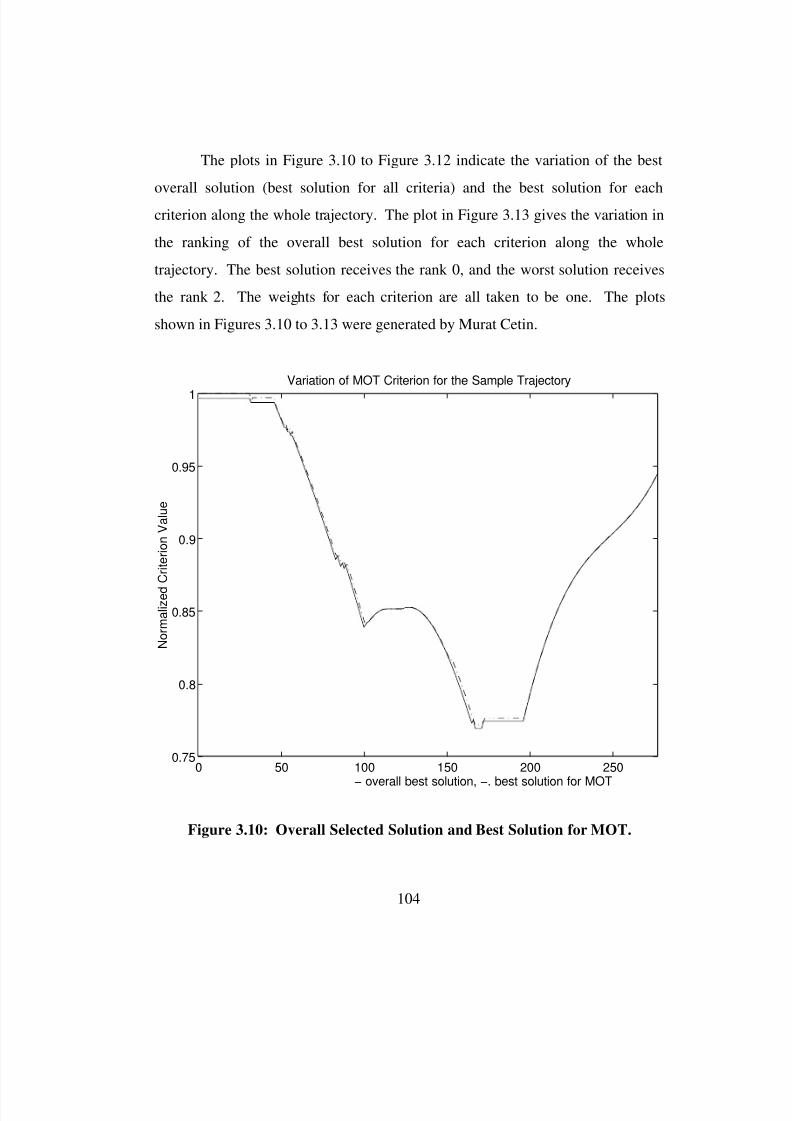
8/3/2019 Chetan Kapoor Dissertation
http://slidepdf.com/reader/full/chetan-kapoor-dissertation 128/612
104
The plots in Figure 3.10 to Figure 3.12 indicate the variation of the best
overall solution (best solution for all criteria) and the best solution for each
criterion along the whole trajectory. The plot in Figure 3.13 gives the variation in
the ranking of the overall best solution for each criterion along the whole
trajectory. The best solution receives the rank 0, and the worst solution receives
the rank 2. The weights for each criterion are all taken to be one. The plots
shown in Figures 3.10 to 3.13 were generated by Murat Cetin.
0 50 100 150 200 2500.75
0.8
0.85
0.9
0.95
1
− overall best solution, −. best solution for MOT
N o r m a l i z e d
C r i t e r i o n V a l u e
Variation of MOT Criterion for the Sample Trajectory
Figure 3.10: Overall Selected Solution and Best Solution for MOT.
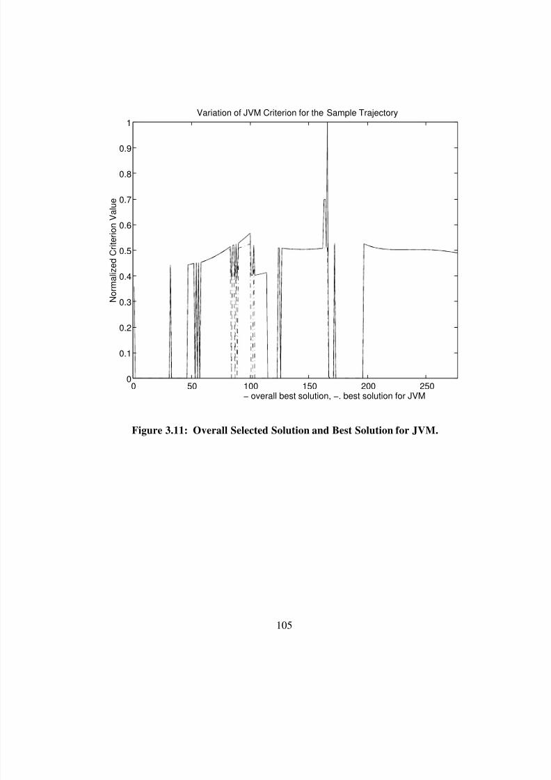
8/3/2019 Chetan Kapoor Dissertation
http://slidepdf.com/reader/full/chetan-kapoor-dissertation 129/612
105
0 50 100 150 200 2500
0.1
0.2
0.3
0.4
0.5
0.6
0.7
0.8
0.9
1
− overall best solution, −. best solution for JVM
N o r m a l i z e d C r i t e r i o n V a l u e
Variation of JVM Criterion for the Sample Trajectory
Figure 3.11: Overall Selected Solution and Best Solution for JVM.
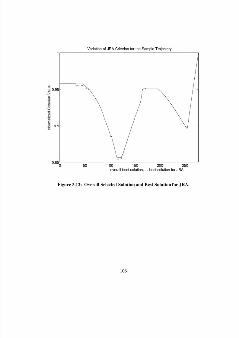
8/3/2019 Chetan Kapoor Dissertation
http://slidepdf.com/reader/full/chetan-kapoor-dissertation 130/612
106
0 50 100 150 200 2500.85
0.9
0.95
1
− overall best solution, −. best solution for JRA
N o r m a l i z e d C r i t e r i o n V a l u e
Variation of JRA Criterion for the Sample Trajectory
Figure 3.12: Overall Selected Solution and Best Solution for JRA.

8/3/2019 Chetan Kapoor Dissertation
http://slidepdf.com/reader/full/chetan-kapoor-dissertation 131/612
107
0 50 100 150 200 2500
1
2Ranking of the overall best solution wrt MOT Criterion
0 50 100 150 200 2500
1
2Ranking of the overall best solution wrt JVM Criterion
0 50 100 150 200 2500
1
2Ranking of the overall best solution wrt JRA Criterion
Figure 3.13: Variation in Ranking of the Overall Best Solution along the
Trajectory for Individual Criterion.
Figure 3.13 shows that though there is no significant tendency, the chosen
solution follows the best solution along most of the trajectory for each of the
criteria. Deviations in either one of the criteria do occur in critical regions where
the particular criterion is reaching a minimum or maximum. Differing from usinga linear combination of normalized criteria values, using ranks offers simplicity
and avoidance of trying to minimize the average of unrelated criteria. The “Rank
options” scheme, thus, uses the preference due to the median criterion (as opposed
8/3/2019 Chetan Kapoor Dissertation
http://slidepdf.com/reader/full/chetan-kapoor-dissertation 132/612
108
to the average) and is not affected by the outliners (by the magnitudes of the
farthest points from the median) as the linear combination of criteria values
would.
3.5.3. Performance Comparison with Hooper’s [1994] Scheme
This sample demonstration of the hybrid inverse scheme was developed
using the software architecture that is being developed as a part of this research.
The application was executed in real-time on VxWorks and used to control the
left-arm of the KB1207 Robotics Research Dual Arm robot. The application was
also executed in simulation on a SUN SPARC 20-61 running the Solaris
operating system. For the inverse computation in this experiment, an aggregate
error at the end-effector was defined as:
E E E T trans rot = +
where,
E T is the total error,
E trans is the translational error in millimeters,
is the scaling factor,
E rot is the rotational error in radians.
Different values of E T were used to experimentally determine some
operational characteristics of the hybrid scheme. These include the operational
frequency of the inverse solution for real-time control and for simulation. The
results are listed in Table 3.1.
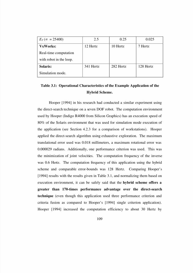
8/3/2019 Chetan Kapoor Dissertation
http://slidepdf.com/reader/full/chetan-kapoor-dissertation 133/612
109
Hooper [1994] in his research had conducted a similar experiment using
the direct-search technique on a seven DOF robot. The computation environment
used by Hooper (Indigo R4000 from Silicon Graphics) has an execution speed of
80% of the Solaris environment that was used for simulation mode execution of
the application (see Section 4.2.3 for a comparison of workstations). Hooper
applied the direct-search algorithm using exhaustive exploration. The maximum
translational error used was 0.018 millimeters, a maximum rotational error was0.000029 radians. Additionally, one performance criterion was used. This was
the minimization of joint velocities. The computation frequency of the inverse
was 0.6 Hertz. The computation frequency of this application using the hybrid
scheme and comparable error-bounds was 128 Hertz. Comparing Hooper’s
[1994] results with the results given in Table 3.1, and normalizing them based on
execution environment, it can be safely said that the hybrid scheme offers a
greater than 170-times performance advantage over the direct-search
technique (even though this application used three performance criterion and
criteria fusion as compared to Hooper’s [1994] single criterion application).
Hooper [1994] increased the computation efficiency to about 30 Hertz by
E T ( = 25400) 2.5 0.25 0.025
VxWorks:Real-time computation
with robot in the loop.
12 Hertz 10 Hertz 7 Hertz
Solaris:
Simulation mode.
341 Hertz 282 Hertz 128 Hertz
Table 3.1: Operational Characteristics of the Example Application of the
Hybrid Scheme.
8/3/2019 Chetan Kapoor Dissertation
http://slidepdf.com/reader/full/chetan-kapoor-dissertation 134/612
110
incorporating a closed-form solution for the three-jointed wrist of the seven DOF
arm. This step reduced the generality of the solution.
3.6. Summary
An extension to Hooper’s [1994] scheme for criteria-based inverse
kinematics was proposed in this chapter.
This scheme has two steps. First the candidate inverse kinematics
solutions are generated. This is accomplished by a two-level “generate-options”
scheme. The first level is the selection of a full-rank sub-matrix of the Jacobian
matrix and solving for a manipulator configuration to satisfy the end-effector
constraints. The second level involves generating candidate inverse kinematics
solutions around the base configurations found at the first level through the “self-
motion” of the manipulator. After the candidate solutions are generated, the best
solution is selected through the so-called “rank-options” scheme. Within this
scheme, each solution is ranked for each criterion. At the end, the ranks for each
solution in each of the criterion are summed and the solution with the lowest (or
highest rank) is picked as the inverse kinematics solution.
Overall, this redundancy resolution scheme does not promise any local or
global optimalities. However, the modeling of the redundancy resolution in
robotics with this scheme allows better concentration on the multicriteria
optimization aspect.
Thus, once the optimization is freed from the inverse kinematics solution
by generating options using the robot’s self-motion, alternative formulations that
will make use of linear or nonlinear programming techniques can be applied to
the resolution of redundancy in real-time. Further research in this area is currently
being conducted at the Robotics Research Group to overcome the limitations of
this scheme.

8/3/2019 Chetan Kapoor Dissertation
http://slidepdf.com/reader/full/chetan-kapoor-dissertation 135/612
111
Chapter Four
4. Development, Execution, and Test Environment
A primary goal of this research was the development of operational
software components for advanced robotics. These components were to exhibit
reuse through generality and extensibility. Additionally, the functionality of these
software components were to be tested on a physical robot and in simulation.
Thus, it was necessary to appropriately select a development, an execution, and a
test environment for the software. The software development environment
includes the computer hardware and software required to develop source code.
This includes the programming language, operating system, software design tools,
and organizational tools. Additionally, pre-made vendor supplied software
components are used to facilitate software development. The software execution
environment includes the computer hardware on which the programs execute and
the operating system the programs use. The test environment includes the
physical robotic hardware the programs control, the simulation computer
(hardware and software), and the peripheral equipment (for example, manualcontrollers) that facilitate robot operation.
Ideally the selection of the software development environment and the
software execution environment should be independent of each other. However,
8/3/2019 Chetan Kapoor Dissertation
http://slidepdf.com/reader/full/chetan-kapoor-dissertation 136/612
112
this is extremely difficult to do while remaining practical. The reason for this is
that even though commercial vendors support a wide array of development
environments, the supported environments rarely support all possible execution
platforms (CPU type, computer board type, bus type, etc.). Thus, though a
designer may find the right development environment, the desired execution
environment would rarely be supported. As a part of this research, it was
necessary to resolve these conflicts. The approach taken involved the
identification of required characteristics of the various sub-systems. Based on
these characteristics, the best available sub-systems were identified. Once this
was done, vendors were located who best satisfied the needs of the various sub-
systems that were identified. Iteration was used at this point to resolve conflicts.
The following sections explain the selection process for the software
development and execution environments and their sub-systems. The criteria
involved in the selection process and the options considered are explained.
Finally, the test environment is explained and then managerial and organizational
issues faced in the software development process are outlined.
4.1. Development and Execution Environment Types
A software designer can take two paths while selecting a software
development and execution environment. The path taken affects the cost of the
environment, the complexity of the development process, and the end product.
The following sub-sections explain the two available options.
4.1.1. Self-Hosted Systems
The best way to explain a self-hosted system is through an example. A
self-hosted system is generally what most software developers use for their
software development and execution. A personal computer that is used for

8/3/2019 Chetan Kapoor Dissertation
http://slidepdf.com/reader/full/chetan-kapoor-dissertation 137/612
113
programming and for the execution of the program is a self-hosted system. In
other words, a self hosted system offers a development and execution
environment in one unit as illustrated in Figure 4.1. Generally, a self hosted
system is characterized by adequate memory and hard-disk space and a processor
that is fast enough for efficient software development.
Applications that do not have space constraints and thus can support a
“full-blown” computer system should use self hosted systems. The various
advantages of a self-hosted system are:
• They have a higher price/performance ratio. This is primarily because of the
large quantity of these systems in the market.
• The most sophisticated technology in computing is generally first made
available on computers using a self hosted development environment. This
includes the latest in operating systems, CPU’s, and software development
tools.
• The software development process is simpler and the user needs to become
familiar with only one system.The disadvantages of a self-hosted system are:
• The software development tools on the self-hosted system may require more
resources (hard disk, memory, processing power) than what may be necessary
Figure 4.1: A Self-Hosted System.
Software Development
Environment
SoftwareExecution
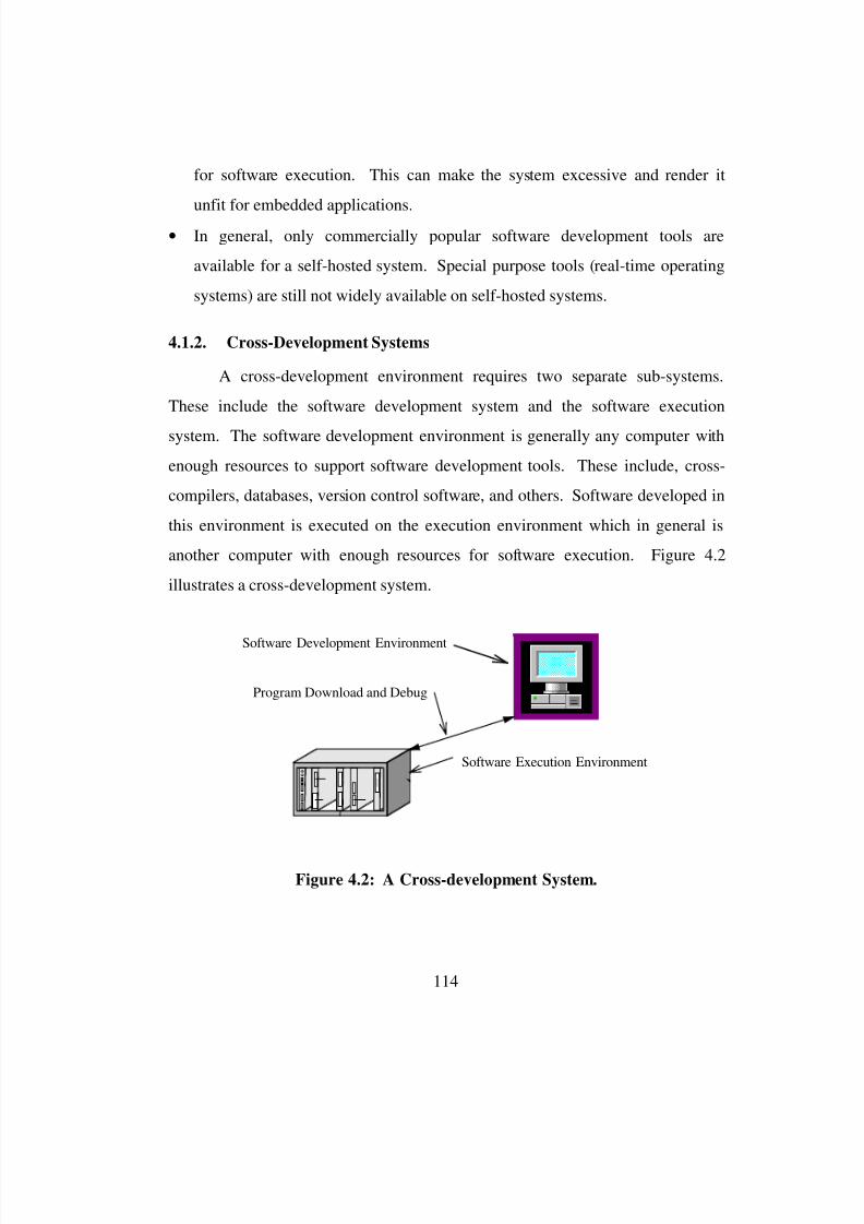
8/3/2019 Chetan Kapoor Dissertation
http://slidepdf.com/reader/full/chetan-kapoor-dissertation 138/612
114
for software execution. This can make the system excessive and render it
unfit for embedded applications.
• In general, only commercially popular software development tools are
available for a self-hosted system. Special purpose tools (real-time operating
systems) are still not widely available on self-hosted systems.
4.1.2. Cross-Development Systems
A cross-development environment requires two separate sub-systems.
These include the software development system and the software execution
system. The software development environment is generally any computer with
enough resources to support software development tools. These include, cross-
compilers, databases, version control software, and others. Software developed in
this environment is executed on the execution environment which in general is
another computer with enough resources for software execution. Figure 4.2
illustrates a cross-development system.
Software ExecutionEnvironment
Software DevelopmentEnvironment
Program Downoladand Debug
Software Development Environment
Software Execution Environment
Program Download and Debug
Figure 4.2: A Cross-development System.
8/3/2019 Chetan Kapoor Dissertation
http://slidepdf.com/reader/full/chetan-kapoor-dissertation 139/612
115
The advantages of using a cross-development environment include:
•
A single development environment can be used to develop executableprograms for different execution environments.
• The execution environment can have limited resources and can thus be
packaged compactly. An example of this is the embedded computer in a
microwave oven. The software for this computer is developed on a larger and
better equipped computer. Once the software is developed, an executable
version is then downloaded to the embedded computer.
• Commercially, a majority of real-time operating systems are geared towards
cross-development environments.
The disadvantages of a cross-development environment are:
• Software development tools are more expensive as compared to tools for self-
hosted systems (generally personal computers and workstations). Also, the
state-of-the-art software development tools may not be available for cross-
development environments.
• Cross-development is more complex and is not as integrated as development
for self-hosted systems.
4.2. Development Environment Selection
The software development environment constitutes
• the software design methodology,
• the programming language,
• the software development tools (computer aided software engineering
(CASE), compilers, debuggers, software organization tools, etc.),
• the operating system used to facilitate software development, and
• the computer hardware on which the software is developed.
8/3/2019 Chetan Kapoor Dissertation
http://slidepdf.com/reader/full/chetan-kapoor-dissertation 140/612
116
Amongst these, the software development tools have the maximum effect
on the quality of the software. Generally, the computer hardware is selected based
on the availability of software development tools and the price/performance ratio
of the hardware. The following sections discuss the various systems that
constitute the software development environment and the issues involved in their
selection.
4.2.1. Software Design Methodology
Currently there are two predominant software design methodologies.
These are structured design and object-oriented design, with the latter rapidly
gaining in popularity. Functional decomposition characterizes structured design.
In functional decomposition the program is broken down into sub-routines (or
procedures). These sub-routines act as instructions that act on data flowing
through them. As the data goes through the sub-routines, it undergoes
transformations. Generally, programming with languages like FORTRAN, C, and
Pascal constitutes structured programming.
The other software design methodology that was considered was object-
oriented design. Object-oriented design professes the decomposition of the
software using objects. Unlike sub-routines (which just hold instructions), objects
hold instructions and data together. This leads to a very modular and self-
contained design of software components. For example, a matrix object will hold
the elements of the matrix, the size of the matrix, and functionality for inverting,
transposing, and multiplying matrices. Additionally, object-oriented design
promotes software reuse through a construct called inheritance. Usinginheritance, a new object (child) can be created by deriving it from an existing
object (parent). The child object inherits all the functionality of the parent. This
8/3/2019 Chetan Kapoor Dissertation
http://slidepdf.com/reader/full/chetan-kapoor-dissertation 141/612
117
inherited functionality can either be modified or even new functionality can be
added. Section 2.5.1.2 provides more details on object-oriented design.
The goal of this research was to develop a reusable software architecture
for advanced robots. This architecture should support modularity and rapid-
prototyping. From literature and experience it was evident that relative to
structured design, object-oriented design offered the advantages of modularity,
encapsulation, standard interfaces, abstraction, reuse, extensibility, and
maintainability (see Section 2.5.2.1 for more details). Because of these
advantages, object-oriented design was chosen as the primary design
methodology for this research.
4.2.2. Language Selection
A computer programming language is a means of describing to the
computer the task to be accomplished. Examples of popular computer
programming languages are C, C++, FORTRAN, Pascal, and BASIC. As a part
of this research, it was necessary to select a programming language for
implementation of the proposed software architecture. The various criteria that
were used in judging different programming languages were:
• Support for object-oriented programming.
• Availability.
• Performance.
• Flexibility.
• Support for low-level and high-level programming.
• Compatibility with other programming languages.
• User preference (developers at the Robotics Research Group).
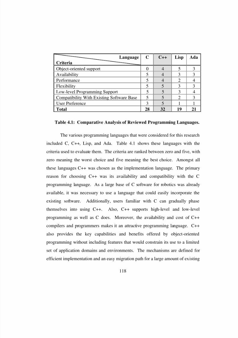
8/3/2019 Chetan Kapoor Dissertation
http://slidepdf.com/reader/full/chetan-kapoor-dissertation 142/612
118
The various programming languages that were considered for this research
included C, C++, Lisp, and Ada. Table 4.1 shows these languages with the
criteria used to evaluate them. The criteria are ranked between zero and five, with
zero meaning the worst choice and five meaning the best choice. Amongst all
these languages C++ was chosen as the implementation language. The primary
reason for choosing C++ was its availability and compatibility with the Cprogramming language. As a large base of C software for robotics was already
available, it was necessary to use a language that could easily incorporate the
existing software. Additionally, users familiar with C can gradually phase
themselves into using C++. Also, C++ supports high-level and low-level
programming as well as C does. Moreover, the availability and cost of C++
compilers and programmers makes it an attractive programming language. C++
also provides the key capabilities and benefits offered by object-oriented
programming without including features that would constrain its use to a limited
set of application domains and environments. The mechanisms are defined for
efficient implementation and an easy migration path for a large amount of existing
LanguageCriteria C C++ Lisp Ada
Object-oriented support 0 4 5 3
Availability 5 4 3 3
Performance 5 4 2 4
Flexibility 5 5 3 3
Low-level Programming Support 5 5 3 4
Compatibility With Existing Software Base 5 5 2 3
User Preference 3 5 1 1
Total 28 32 19 21
Table 4.1: Comparative Analysis of Reviewed Programming Languages.
8/3/2019 Chetan Kapoor Dissertation
http://slidepdf.com/reader/full/chetan-kapoor-dissertation 143/612
119
C software and programmers. Features that would result in performance penalties
have not been included in the language. Thus, C++ does not strictly enforce
object-oriented programming [Jordan, 1990]. This is a drawback of C++ but it
can be used to design efficient and deterministic programs. Determinism and
efficiency are required for operational and real-time software.
4.2.3. Operating System Selection
The operating system provides a software interface to access the
functionality of the computer hardware. The selection of the operating system for
the development environment is not critical and it depends mainly on user
preferences, support for software development tools, and the desired computer
hardware. It should be noted that for a self-hosted system the operating system
also provides a software execution environment. In this case the functionality of
the operating system is critical to the performance of the software and is discussed
in the section on execution environment selection (see Section 4.3).
Thus, as far as the selection of an operating system to support software
development is concerned, the relevant criteria are:
• User preference.
• Support for software development tools (compilers, debuggers, version
control, etc.)
• Computer hardware supported.
The two options considered for a software development operating system
were Windows NT and UNIX. Based on user preferences and cost, Windows NT
was a better option. As far as the variety of computer hardware and the support
for software development tools is concerned, it was noted that UNIX was a better
option. As the availability of software development tools was crucial to this
research, UNIX was selected as the operating system for software development.
8/3/2019 Chetan Kapoor Dissertation
http://slidepdf.com/reader/full/chetan-kapoor-dissertation 144/612
120
However the availability of software development tools on Windows NT is rising.
If faced with a similar decision in the future, Windows NT may prove to be a
better option than UNIX.
After selecting UNIX as the operating system for software development, it
was necessary to pick a UNIX vendor who offered the best price/performance
ratio and the maximum support for development tools. The various criteria that
were used to select a UNIX vendor were:
• Multi-user environment to allow simultaneous code development.
• Robust system with enough security.
• Built in networking.
• C++ development environment support.
• Graphical software development tools (debuggers).
• Availability of Computer Aided Software Engineering (CASE) tools for
software analysis and design.
• Strong customer support.
• Popularity and user preference.
• Efficiency of the computer hardware.
The various options that were considered for the software development
environments that supported UNIX are shown in Table 4.2. The popularity and
the availability of software development tools is ranked on a range of 1 to 5, with
1 implying the minimum availability and 5 the maximum. The prices shown are
1994 academic prices.

8/3/2019 Chetan Kapoor Dissertation
http://slidepdf.com/reader/full/chetan-kapoor-dissertation 145/612
121
Among the various UNIX workstations under consideration (see Table
4.2), it was seen that the uniprocessor SUN workstation offered the best
price/performance ratio and best supported software development tools. Hence it
was selected as the software development environment. This workstation
supports the Solaris (a commercial version of UNIX) operating system.
4.3. Execution Environment Selection
The software execution environment includes the computer hardware on
which the software executes and the operating system this hardware supports forefficient software execution. The following sections outline the details of the
selection process for the operating system and the computer hardware.
Criteria
Workstation
ProcessorSpeed SoftwareDevelopment
Tools
Popularity(ranking) Price(approx.)Dollars
SGI Indy MIPSR4400SC 150 MHz
SPECint92 91.7
SPECfp92 97.5
2 4 8,000
SGI Indigo MIPS R4400150 MHz
SPECint92 86.0
SPECfp92 93.2
2 4 19,000
SGI Power Challenge M
R8000 150 MHzSPECint92 108
SPECfp92 310
2 4 22,750
IBM RS6000
Power Station 3BTSPECint92 114
SPECfp92 205
3 3 22,000
SUN SPARC 20-61Singe Processor 60 MHz
SPECint92 89
SPECfp92 102.8
4 2 11,497
SUN SPARC 20-61Dual Processor 60 MHz
SPECint92 89
SPECfp92 102.8
4 2 13,497
DEC ALPHA
Model 700SPECint92 162
SPECfp92 230
3 3 26,000
DEC ALPHA
Model 900SPECint92 189
SPECfp92 264
3 3 37,000
Table 4.2: UNIX Workstations Considered for Software Development.

8/3/2019 Chetan Kapoor Dissertation
http://slidepdf.com/reader/full/chetan-kapoor-dissertation 146/612
122
4.3.1. Operating System Selection
An operating system is the core of present day computers and provides theuser with an environment to manage the low level details of the execution of
software. Some important functions of an operating system are process
management, memory management, and file system management. Popular
examples of operating systems are UNIX, Windows NT, OS/2, etc. Operating
systems provide the software developer with an Applications Programming
Interface (API) which can be used to develop programs that rely on networking,
parallel processing, and graphical user interfaces. The selection of an operating
system was crucial to this research because the proposed software architecture had
to allow for software execution in an operational and simulation environment.
As mentioned in Chapter Two, this research involves developing a
software architecture for the middle, that is, the operational layer of robotic
software. Thus, the operating system should satisfy the requirements for the
operational software layer. Additionally, the selected operating system will also
have to support the development of the lower-most real-time layer of robotic
software and the top-most layer of robot programming. The requirements of these
two layers also must be taken into account as the development of these layers is
crucial to the success of a robotic software architecture. Thus, the demands on the
operating system are characterized by the requirements posed by each layer of the
robotic software. These requirements are:
Robot Programming Layer
• Support for efficient development of a graphical user interface that will assist
in robot programming and operation.
• Networking support for connectivity to other computers that are used for off-
line programming.
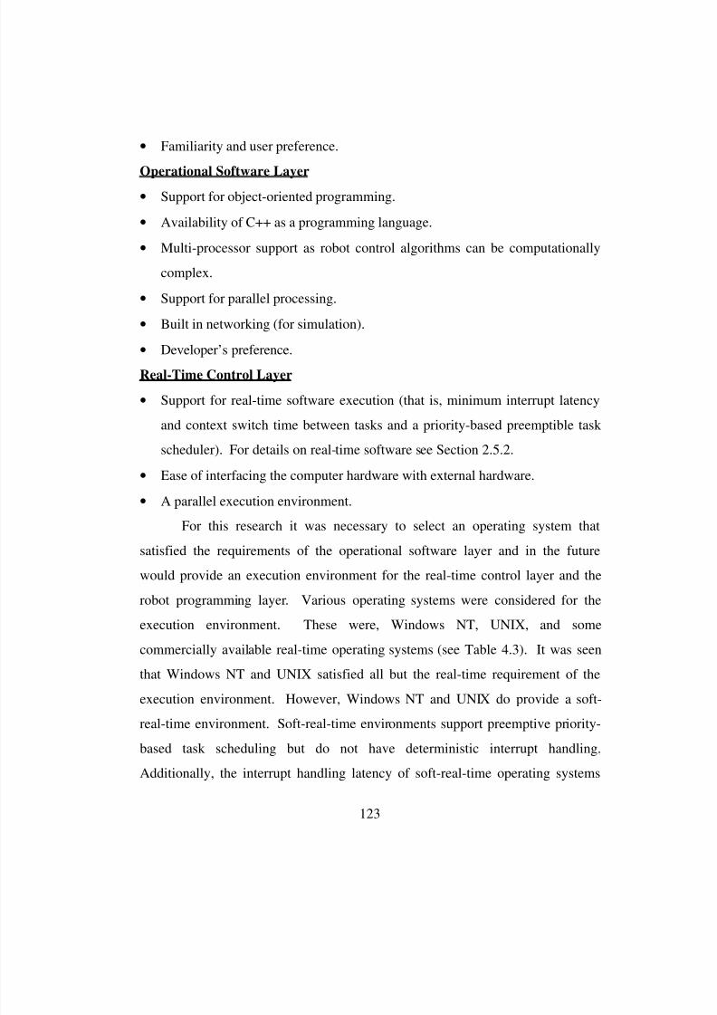
8/3/2019 Chetan Kapoor Dissertation
http://slidepdf.com/reader/full/chetan-kapoor-dissertation 147/612
123
• Familiarity and user preference.
Operational Software Layer• Support for object-oriented programming.
• Availability of C++ as a programming language.
• Multi-processor support as robot control algorithms can be computationally
complex.
• Support for parallel processing.
• Built in networking (for simulation).
•
Developer’s preference.Real-Time Control Layer
• Support for real-time software execution (that is, minimum interrupt latency
and context switch time between tasks and a priority-based preemptible task
scheduler). For details on real-time software see Section 2.5.2.
• Ease of interfacing the computer hardware with external hardware.
• A parallel execution environment.
For this research it was necessary to select an operating system that
satisfied the requirements of the operational software layer and in the future
would provide an execution environment for the real-time control layer and the
robot programming layer. Various operating systems were considered for the
execution environment. These were, Windows NT, UNIX, and some
commercially available real-time operating systems (see Table 4.3). It was seen
that Windows NT and UNIX satisfied all but the real-time requirement of the
execution environment. However, Windows NT and UNIX do provide a soft-
real-time environment. Soft-real-time environments support preemptive priority-
based task scheduling but do not have deterministic interrupt handling.
Additionally, the interrupt handling latency of soft-real-time operating systems
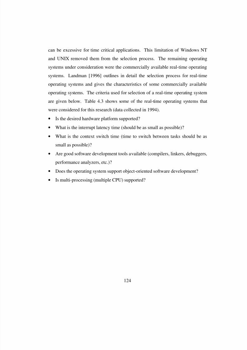
8/3/2019 Chetan Kapoor Dissertation
http://slidepdf.com/reader/full/chetan-kapoor-dissertation 148/612
124
can be excessive for time critical applications. This limitation of Windows NT
and UNIX removed them from the selection process. The remaining operating
systems under consideration were the commercially available real-time operating
systems. Landman [1996] outlines in detail the selection process for real-time
operating systems and gives the characteristics of some commercially available
operating systems. The criteria used for selection of a real-time operating system
are given below. Table 4.3 shows some of the real-time operating systems that
were considered for this research (data collected in 1994).
• Is the desired hardware platform supported?
• What is the interrupt latency time (should be as small as possible)?
• What is the context switch time (time to switch between tasks should be as
small as possible)?
• Are good software development tools available (compilers, linkers, debuggers,
performance analyzers, etc.)?
• Does the operating system support object-oriented software development?
• Is multi-processing (multiple CPU) supported?

8/3/2019 Chetan Kapoor Dissertation
http://slidepdf.com/reader/full/chetan-kapoor-dissertation 149/612
125
VxWorks was selected from all the real-time operating systems that
were evaluated. The primary reasons for this were the availability of software
development tools, a strong track record and acceptance in the industry, support
for a variety of computer hardware, a low interrupt latency, and project
deliverable requirements.
4.3.2. Execution Computer Hardware
Once an operating system software was selected for the execution
environment, it was necessary to select the computer hardware for software
execution. This involved selecting the processor and the computer bus that best
supported the execution hardware. Again, the selection of these was done
Criteria
Name
HostPlatforms TargetProcessors C++Support Multi-Processing Price(discount)
VxWorks SUN, SGI,IBM, PC
PowerPC,MIPS,
Motorola
Yes Yes 25,000(60 %)
Lynx OS Self Hosted System386, 486, SPARC, MVME
Yes No 5000(60 %)
PSoS+m.
SUN, SGI,IBM, PC
Intel,Motorola
Yes Yes 25,000(0 %)
OS-9 UNIX, DOS Motorola,Intel
Yes No 2000
RMKIBM
IBM RS6000
Motorola Yes Yes Not acommercial
product
C Executive UNIX, DOS Intel,Motorola,
MIPS
No No 2,500
VRTX SUN, PC,HP
Intel,Motorola
Yes No 17,000(0 %)
Table 4.3: Commercially Available Real-Time Operating Systems.
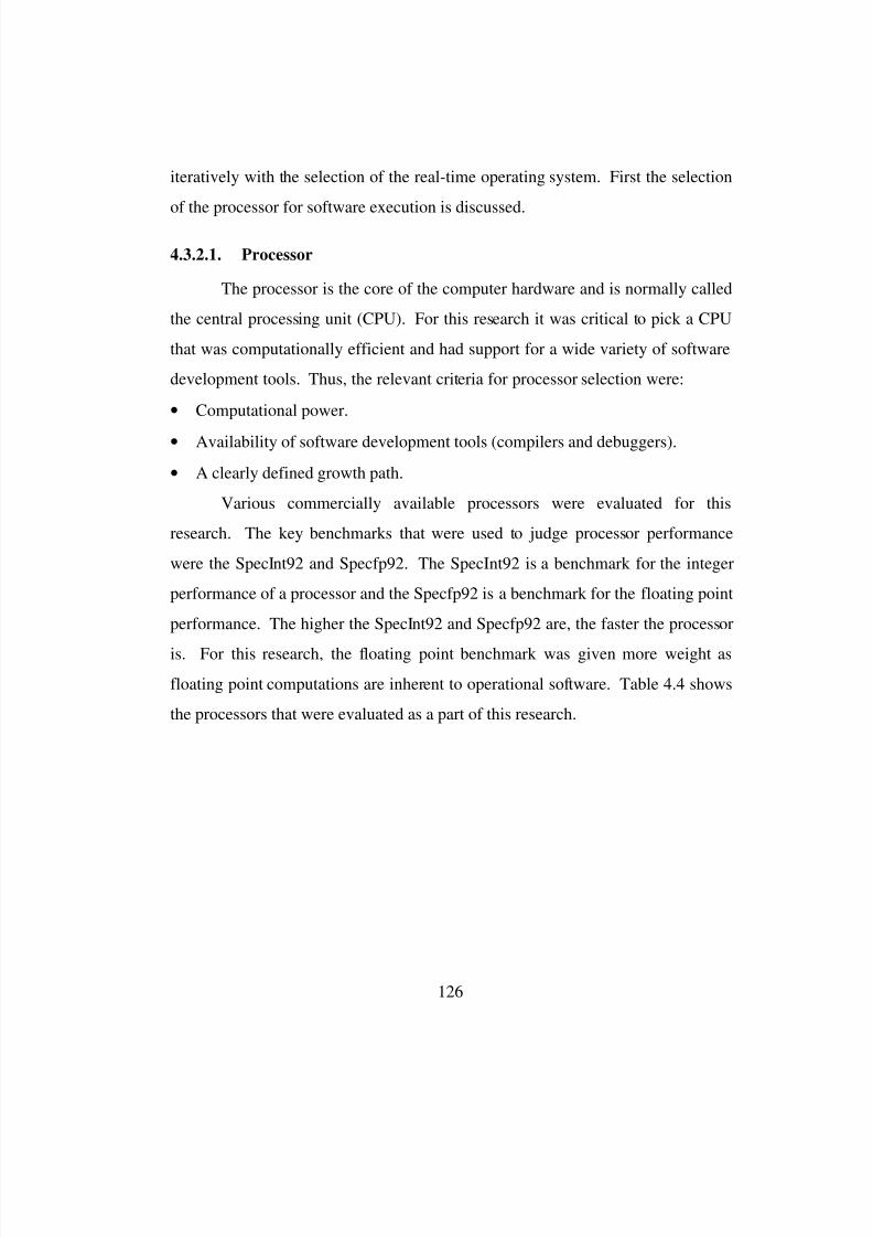
8/3/2019 Chetan Kapoor Dissertation
http://slidepdf.com/reader/full/chetan-kapoor-dissertation 150/612
126
iteratively with the selection of the real-time operating system. First the selection
of the processor for software execution is discussed.
4.3.2.1. Processor
The processor is the core of the computer hardware and is normally called
the central processing unit (CPU). For this research it was critical to pick a CPU
that was computationally efficient and had support for a wide variety of software
development tools. Thus, the relevant criteria for processor selection were:
• Computational power.
• Availability of software development tools (compilers and debuggers).
• A clearly defined growth path.
Various commercially available processors were evaluated for this
research. The key benchmarks that were used to judge processor performance
were the SpecInt92 and Specfp92. The SpecInt92 is a benchmark for the integer
performance of a processor and the Specfp92 is a benchmark for the floating point
performance. The higher the SpecInt92 and Specfp92 are, the faster the processor
is. For this research, the floating point benchmark was given more weight as
floating point computations are inherent to operational software. Table 4.4 shows
the processors that were evaluated as a part of this research.
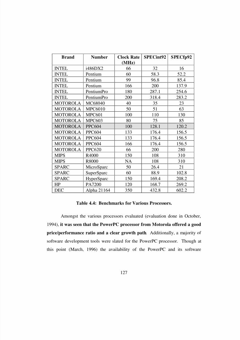
8/3/2019 Chetan Kapoor Dissertation
http://slidepdf.com/reader/full/chetan-kapoor-dissertation 151/612
127
Amongst the various processors evaluated (evaluation done in October,
1994), it was seen that the PowerPC processor from Motorola offered a good
price/performance ratio and a clear growth path. Additionally, a majority of
software development tools were slated for the PowerPC processor. Though at
this point (March, 1996) the availability of the PowerPC and its software
Brand Number Clock Rate(MHz) SPECint92 SPECfp92
INTEL i486DX2 66 32 16
INTEL Pentium 60 58.3 52.2
INTEL Pentium 99 96.8 85.4
INTEL Pentium 166 200 137.9
INTEL PentiumPro 180 287.1 254.6
INTEL PentiumPro 200 318.4 283.2
MOTOROLA MC68040 40 35 23
MOTOROLA MPC6010 50 51 63
MOTOROLA MPC601 100 110 130
MOTOROLA MPC603 80 75 85MOTOROLA PPC604 100 128.1 120.2
MOTOROLA PPC604 133 176.4 156.5
MOTOROLA PPC604 133 176.4 156.5
MOTOROLA PPC604 166 176.4 156.5
MOTOROLA PPC620 66 200 280
MIPS R4000 150 108 310
MIPS R8000 NA 108 310
SPARC MicroSparc 50 26.4 21
SPARC SuperSparc 60 88.9 102.8
SPARC HyperSparc 150 169.4 208.2HP PA7200 120 168.7 269.2
DEC Alpha 21164 350 432.8 602.2
Table 4.4: Benchmarks for Various Processors.
8/3/2019 Chetan Kapoor Dissertation
http://slidepdf.com/reader/full/chetan-kapoor-dissertation 152/612
128
development tools has been delayed. The Intel x86 (Pentium, PentiumPro) family
of processors offers another feasible option.
4.3.2.2. Bus Type
A bus is a medium for transmitting signals from one or more sources to
one or more destinations. It can be used for information transfer within a
computer or between computers and peripheral devices. There are two major
types of buses - computer and instrumentation. The computer bus is the internal
bus that connects the CPU to the various I/O devices and other peripherals
contained within a closed system. The instrumentation bus is used to connect
external devices to each other. The instrumentation bus uses addressable or point-
to-point communication. A VME bus is an example of a computer bus, and
Ethernet is an example of an instrumentation bus. [Potter, 1992]
Once a processor for software execution was selected, it was necessary to
select a bus upon which this processor would be located. The selection of the bus
is crucial to the development of an extensible hardware environment. As the need
arises, more computer boards can be added. These can include CPU modules,
digital I/O cards, etc. Additionally, it was essential that when new hardware was
added, it should couple tightly with the existing hardware. This allows for faster
communication amongst the various hardware modules. An example of this is
when a processor card and a digital I/O card are both located on the same high-
speed bus.
The first issue faced in bus selection is determining the type of bus -
computer or instrumentation. If the devices to be connected have their ownembedded control but have to be supervised by another computer or device, it is
better to use an instrumentation bus. However, if the devices are to be directly
controlled by a computer, then it is better to have a computer bus connect directly
8/3/2019 Chetan Kapoor Dissertation
http://slidepdf.com/reader/full/chetan-kapoor-dissertation 153/612
129
to these devices. Some of the important factors for bus selection are presented
below and Table 4.5 gives an overview of some of the commercially available
buses [Potter, 1992].
• Do the various devices on the bus have their own embedded control?
• Are the various devices on the bus directly controlled by another computer?
• What is the desired data transfer rate?
• How many devices are to be attached on the bus?
• Is the bus addressable and if so, how many address lines are provided by the
bus?
• Do the software development tools support the bus type?
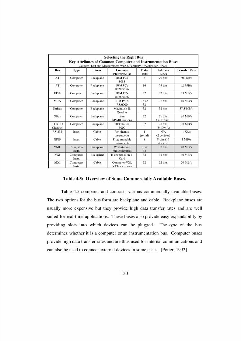
8/3/2019 Chetan Kapoor Dissertation
http://slidepdf.com/reader/full/chetan-kapoor-dissertation 154/612
130
Table 4.5 compares and contrasts various commercially available buses.
The two options for the bus form are backplane and cable. Backplane buses are
usually more expensive but they provide high data transfer rates and are well
suited for real-time applications. These buses also provide easy expandability by
providing slots into which devices can be plugged. The type of the bus
determines whether it is a computer or an instrumentation bus. Computer buses
provide high data transfer rates and are thus used for internal communications and
can also be used to connect external devices in some cases. [Potter, 1992]
Selecting the Right Bus
Key Attributes of Common Computer and Instrumentation BusesSource: Test and Measurement World, February, 1992 [Potter, 1992].
Bus Type Form Common
Platform/Use
Data
Bits
Address
Lines
Transfer Rate
XT Computer Backplane IBM PCs
8088
8 20 bits 800 Kb/s
AT Computer Backplane IBM PCs
80286/386
16 24 bits 1.6 MB/s
EISA Computer Backplane IBM PCs
80386/486
32 32 bits 33 MB/s
MCA Computer Backplane IBM PS/2,
RS/6000
16 or
32
32 bits 40 MB/s
NuBus Computer Backplane Macintosh II,
Quadras
32 32 bits 37.5 MB/s
SBus Computer Backplane Sun
SPARCstations
32 2b bits
(32 virtual)
80 MB/s
TURBO
Channel
Computer Backplane DECstation
5000
32 28 bits
(34 DMA)
98 MB/s
RS-232 Instr. Cable Peripherals,
instruments
1
(serial)
N/A
(2 devices)
1 Kb/s
GPIB Instr. Cable Programmable
instruments
8 8-bits (15
devices)
1 MB/s
VME Computer/
Instr.
Backplane Workstation/
minicomputers
16 or
32
32 bits 40 MB/s
VXI Computer/
Instr.
Backplane Instruments-on-a-
Card
32 32 bits 40 MB/s
MXI Computer/
Instr.
Cable Computer-VXI,
VXI extensions
32 32 bits 20 MB/s
Table 4.5: Overview of Some Commercially Available Buses.
8/3/2019 Chetan Kapoor Dissertation
http://slidepdf.com/reader/full/chetan-kapoor-dissertation 155/612
131
As discussed earlier, this research had to select an execution environment
that supported real-time program execution. It was thus necessary to select a
computer bus that could support high-speed communication between different
hardware modules. Additionally, the availability of computer hardware for the
selected bus had to be analyzed. For example, in this research it was necessary to
connect the execution computer to the physical robot servo-control. Thus, it was
necessary that a hardware bus-to-bus adapter be available that would connect the
execution computer bus to the robot bus. Additionally, the selected bus should be
supported by the selected real-time operating system (in this case VxWorks).
Analyzing the various options, VME was chosen as the bus for the computer
hardware.
4.4. Summary of the Selected Environment
As mentioned earlier, the methodology employed for selection of the
development and execution environment followed two steps. The first step was
the selection of the individual sub-systems in the development and execution
environment. The second step was to iterate over the selected subsystems to
resolve potential conflicts. Eventually, an environment was selected that best
supported software development and execution. This environment is summarized
in Table 4.6.
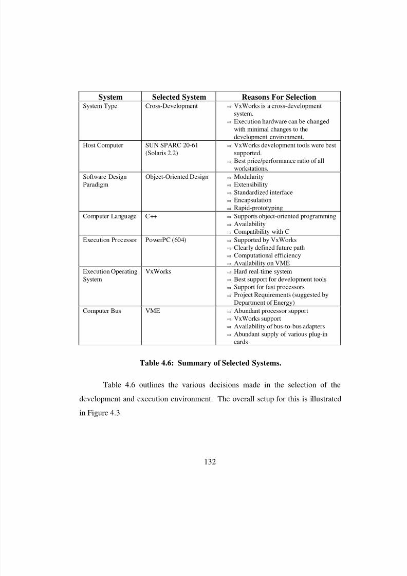
8/3/2019 Chetan Kapoor Dissertation
http://slidepdf.com/reader/full/chetan-kapoor-dissertation 156/612
132
Table 4.6 outlines the various decisions made in the selection of the
development and execution environment. The overall setup for this is illustrated
in Figure 4.3.
System Selected System Reasons For SelectionSystem Type Cross-Development ⇒ VxWorks is a cross-developmentsystem.
⇒ Execution hardware can be changedwith minimal changes to thedevelopment environment.
Host Computer SUN SPARC 20-61(Solaris 2.2)
⇒ VxWorks development tools were bestsupported.
⇒ Best price/performance ratio of allworkstations.
Software DesignParadigm
Object-Oriented Design ⇒ Modularity⇒ Extensibility⇒ Standardized interface
⇒ Encapsulation⇒ Rapid-prototyping
Computer Language C++ ⇒ Supports object-oriented programming⇒ Availability⇒ Compatibility with C
Execution Processor PowerPC (604) ⇒ Supported by VxWorks⇒ Clearly defined future path⇒ Computational efficiency⇒ Availability on VME
Execution OperatingSystem
VxWorks ⇒ Hard real-time system⇒ Best support for development tools⇒ Support for fast processors⇒ Project Requirements (suggested by
Department of Energy)Computer Bus VME ⇒ Abundant processor support
⇒ VxWorks support⇒ Availability of bus-to-bus adapters⇒ Abundant supply of various plug-in
cards
Table 4.6: Summary of Selected Systems.
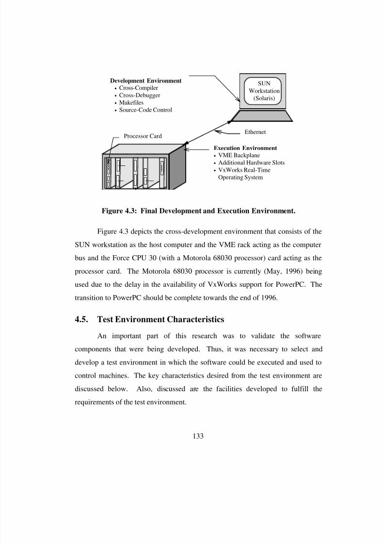
8/3/2019 Chetan Kapoor Dissertation
http://slidepdf.com/reader/full/chetan-kapoor-dissertation 157/612
133
Figure 4.3 depicts the cross-development environment that consists of the
SUN workstation as the host computer and the VME rack acting as the computer
bus and the Force CPU 30 (with a Motorola 68030 processor) card acting as the
processor card. The Motorola 68030 processor is currently (May, 1996) being
used due to the delay in the availability of VxWorks support for PowerPC. Thetransition to PowerPC should be complete towards the end of 1996.
4.5. Test Environment Characteristics
An important part of this research was to validate the software
components that were being developed. Thus, it was necessary to select and
develop a test environment in which the software could be executed and used to
control machines. The key characteristics desired from the test environment are
discussed below. Also, discussed are the facilities developed to fulfill the
requirements of the test environment.
Ethernet
SUNWorkstation
(Solaris)
Development Environment
• Cross-Compiler
• Cross-Debugger• Makefiles• Source-Code Control
Processor Card
Execution Environment
• VME Backplane• Additional Hardware Slots• VxWorks Real-Time
Operating System
Figure 4.3: Final Development and Execution Environment.
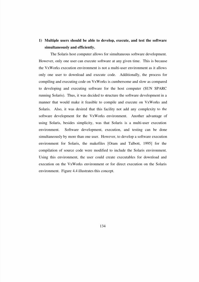
8/3/2019 Chetan Kapoor Dissertation
http://slidepdf.com/reader/full/chetan-kapoor-dissertation 158/612
134
1) Multiple users should be able to develop, execute, and test the software
simultaneously and efficiently.
The Solaris host computer allows for simultaneous software development.
However, only one user can execute software at any given time. This is because
the VxWorks execution environment is not a multi-user environment as it allows
only one user to download and execute code. Additionally, the process for
compiling and executing code on VxWorks is cumbersome and slow as compared
to developing and executing software for the host computer (SUN SPARC
running Solaris). Thus, it was decided to structure the software development in a
manner that would make it feasible to compile and execute on VxWorks and
Solaris. Also, it was desired that this facility not add any complexity to the
software development for the VxWorks environment. Another advantage of
using Solaris, besides simplicity, was that Solaris is a multi-user execution
environment. Software development, execution, and testing can be done
simultaneously by more than one user. However, to develop a software execution
environment for Solaris, the makefiles [Oram and Talbott, 1995] for the
compilation of source code were modified to include the Solaris environment.
Using this environment, the user could create executables for download and
execution on the VxWorks environment or for direct execution on the Solaris
environment. Figure 4.4 illustrates this concept.
8/3/2019 Chetan Kapoor Dissertation
http://slidepdf.com/reader/full/chetan-kapoor-dissertation 159/612
135
The one limitation of this environment was that the code could only be
executed in simulation mode on the Solaris environment. This was because the
hardware connection from the SUN workstation to the physical robot was not
developed. Additionally, Solaris is not suited for real-time software execution.
2) The testing environment should support simulation.
The software development cycle can be roughly characterized by three
stages. These are compile, test, and debug. For maximum productivity, it is
necessary to have an efficient test environment. This productivity is significantly
lowered when software being developed is used to control physical robotic
manipulators. This is because the use of a physical robot is expensive, dangerous,
and cumbersome. To increase the efficiency of the test environment, it was
necessary to allow for the integration of a simulation environment. The
simulation environment is even more important when Solaris is used as an
execution environment. As mentioned earlier, this is because the multi-user
execution environment provided by Solaris supports only simulation.
The simulation environment selected for this research involved using
three-dimensional (3D) graphical simulations of robotic manipulators in place of
Development Environment
• SUN Sparc running Solaris
• Multi-User Development• Source Code can be
Compiled for Solaris orVxWorks
Host Computer
C++ Source Code
• Cross-Compiled for
VxWorks Execution• Compiled forExecution on Solaris
VxWorks Execution
• Executes Code Compiledfor VxWorks
• Single-User Execution
Solaris Execution
• Executes Code
Compiled for Solaris• Multi-user Execution
VME Rack
Figure 4.4: Multi-user Execution and Test Environment.

8/3/2019 Chetan Kapoor Dissertation
http://slidepdf.com/reader/full/chetan-kapoor-dissertation 160/612
136
physical robots. The graphical simulations were implemented on stand-alone
computers. ROBOCAD, a 3D modular robot modeling software was used to
create the robot models [Hooper, 1990]. Additionally, complex models of robots
that were not possible in ROBOCAD could be implemented using high-level
graphics libraries developed by the author (see Appendix D). These libraries offer
software components for procedural modeling of 3D shapes. Additionally, these
libraries encapsulate the functionality of the window manager and provide a user-
friendly interface for viewing manufacturing cells. The shapes provided in this
library are basic quadrics (cylinders, spheres, etc.), cones, extrusions, and sweeps.
Using these components, complex 3D graphical environments can be modeled.
Various hardware options were offered for the simulation environment. The first
was the use of Silicon Graphics computers. Both ROBOCAD and the graphics
libraries were available on this platform. The authors graphics libraries (see
Appendix D) were also available on personal computers running Windows NT.
Once the simulation environment was in place, the next step was to
provide a communication interface between the execution computer and the
simulation computer. The requirements for the communication interface were:
• high-speed,
• use of existing networks,
• point-to-point configuration,
• easy reconfiguration, and
• availability on different computer platforms (Solaris, VxWorks, Windows NT,
Silicon Graphics).
To fulfill these requirements, Ethernet was chosen as the hardware
medium of communications. Transmission Control Protocol (TCP) sockets
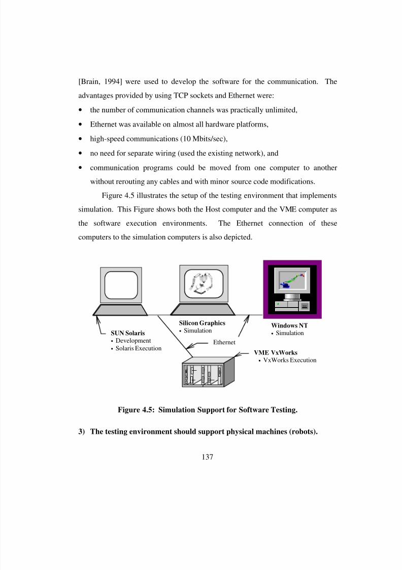
8/3/2019 Chetan Kapoor Dissertation
http://slidepdf.com/reader/full/chetan-kapoor-dissertation 161/612
137
[Brain, 1994] were used to develop the software for the communication. The
advantages provided by using TCP sockets and Ethernet were:
• the number of communication channels was practically unlimited,
• Ethernet was available on almost all hardware platforms,
• high-speed communications (10 Mbits/sec),
• no need for separate wiring (used the existing network), and
• communication programs could be moved from one computer to another
without rerouting any cables and with minor source code modifications.
Figure 4.5 illustrates the setup of the testing environment that implements
simulation. This Figure shows both the Host computer and the VME computer as
the software execution environments. The Ethernet connection of these
computers to the simulation computers is also depicted.
3) The testing environment should support physical machines (robots).
Figure 4.5: Simulation Support for Software Testing.
Ethernet
SUN Solaris• Development• Solaris Execution
Silicon Graphics
• SimulationWindows NT
• Simulation
VME VxWorks
• VxWorks Execution
8/3/2019 Chetan Kapoor Dissertation
http://slidepdf.com/reader/full/chetan-kapoor-dissertation 162/612
138
The purpose of this research was to design and develop software
components that could be used to control advanced robotic machines. The real
test for these components was in controlling physical machines (robots). Thus, it
was necessary to make available robotic hardware and the corresponding
interfacing software. This interfacing software would provide a substitute for the
real-time control layer (see Chapter Two) of the robotic software. The operational
software components developed as a part of this research communicate with the
physical hardware through this real-time control layer. Also, as the components
developed as a part of this research were to be used for advanced robots, it was
necessary to provide a test environment that included advanced as well as
standard industrial robots.
Currently, three robotic manipulators are available for demonstrations and
testing of the software. The first and the oldest of these is the Puma Mark II 500
Series six DOF manipulator. The operational software layer communicates with
this robot using an RS-232 connection. The other robot used for this research is a
heavy duty T3-786 industrial robot from Cincinnati Milacron. The operational
software layer communicates using an RS-232 with this robot in supervisory
mode. The third, and the most advanced robot available for this research is the
seventeen DOF dual-arm robotic manipulator from Robotics Research
Corporation. This robot arm consists of two seven DOF arms and a three DOF
torso. The operational software layer communicates with this robot through a
real-time control layer. The dual-arm servo-level controller comes equipped with
an interface that can be used to send position, velocity, or torque set-points to the
servos. The computer used for the servo-control of the dual-arm uses Multibus as
the computer bus. Thus, to connect the execution environment (VME rack,
processor card, VxWorks) a VME-to-Multibus hardware adapter was used. Using
this adapter, memory locations on the servo-level computer of the dual-arm robot
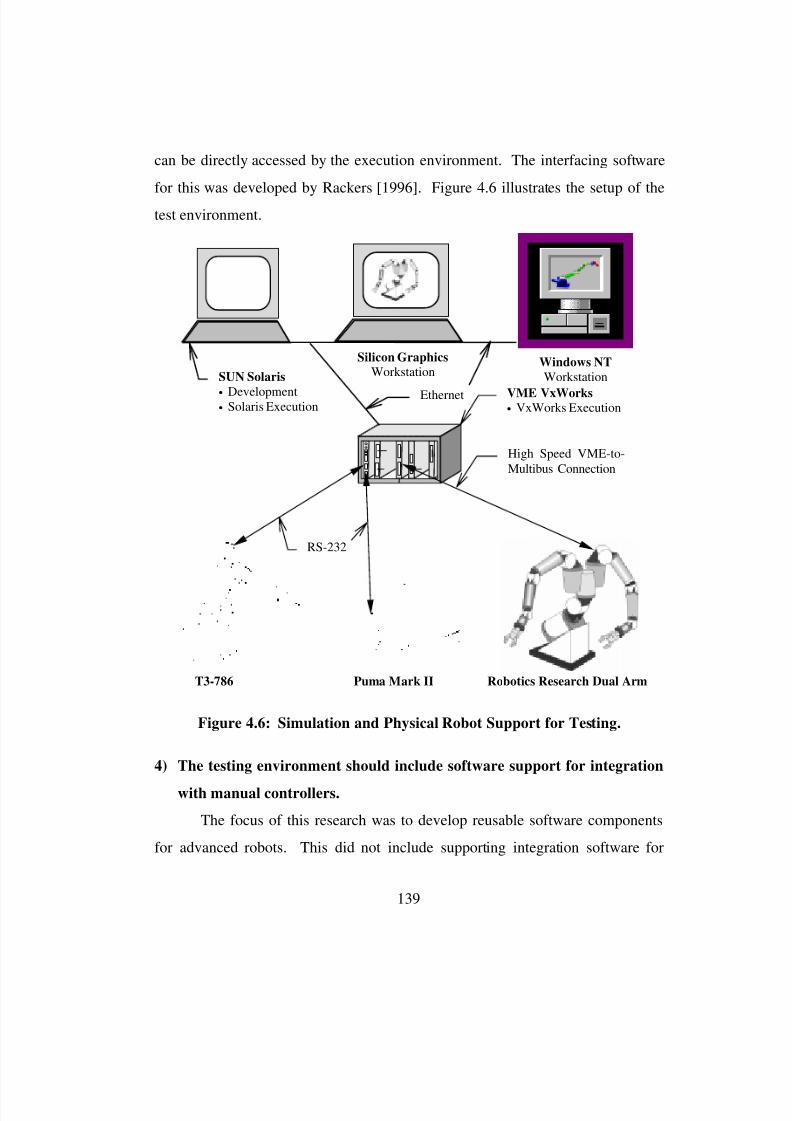
8/3/2019 Chetan Kapoor Dissertation
http://slidepdf.com/reader/full/chetan-kapoor-dissertation 163/612
139
can be directly accessed by the execution environment. The interfacing software
for this was developed by Rackers [1996]. Figure 4.6 illustrates the setup of the
test environment.
Figure 4.6: Simulation and Physical Robot Support for Testing.
4) The testing environment should include software support for integration
with manual controllers.
The focus of this research was to develop reusable software components
for advanced robots. This did not include supporting integration software for
Ethernet
SUN Solaris
• Development• Solaris Execution
Silicon Graphics
WorkstationWindows NT
Workstation
VME VxWorks• VxWorks Execution
RS-232
High Speed VME-to-Multibus Connection
T3-786 Puma Mark II Robotics Research Dual Arm

8/3/2019 Chetan Kapoor Dissertation
http://slidepdf.com/reader/full/chetan-kapoor-dissertation 164/612
140
connecting to peripheral equipment. Then why is the requirement for integration
software for manual controllers placed in the test environment? There are a few
reasons why it was necessary to provide integration software for manual
controllers. These are:
• Manual controllers are an integral part of robotics and are essential for
meaningful teleoperation.
• The integration of manual controllers was important because an environment
was needed to evaluate and test various manual controllers. The core of this
research already provided an environment for controlling different robotic
manipulators. So the next logical step was to make this environment
accessible to manual controllers. Also, if the claims of reusability and rapid-
prototyping capability of the software components were true, the integration
of manual controllers would not involve extensive program development.
• It was realized that a manual controller provided an efficient interface for
controlling the robot as compared to teach-pendant type approaches.
• Due to the object-oriented nature of the software components developed for
this research, it was realized that any new development for the integration
software would be minimal.
Thus, once it was determined that manual controllers should be integrated
into the operational software architecture, the next step was to choose a path that
supported efficient integration. Two options were considered for this. These
were:
1) The manual controllers should plug-in directly to the execution environment,
that is, the VME rack. Once the manual controller hardware is plugged in, the
next step would be to write the software that interfaces with the hardware.
8/3/2019 Chetan Kapoor Dissertation
http://slidepdf.com/reader/full/chetan-kapoor-dissertation 165/612
141
This approach is based on a centralized model of control, with the center
being the VME rack.
2) The second approach is to use a separate computer into which the manual
controllers are connected. The software for interfacing with the manual
controllers executes on this computer. A communication link can then be
provided between the manual controller computer and the VME rack on
which the operational software executes. This path follows the distributed
approach, an approach that proposes the use of loosely coupled localized
controllers connected through high-speed communications.
The advantages and disadvantages of these approaches are as follows:
• In the first approach the software execution takes place under VxWorks
providing for better real-time control.
• The first approach provides an integrated environment for the manual
controller software.
• The first approach, that is, the centralized approach goes against the concept
of modularity. The distributed approach uses localized control and thus
provides for a well defined interface.
• The first approach uses VxWorks. As mentioned earlier, VxWorks is a single
user execution environment. Thus, this approach puts more demands on the
available resources.
• The second approach uses a separate computer. This characteristic can be
used to select a computer that has the best price/performance ratio and has
more efficient software development tools.
Considering the advantages and disadvantages of the two approaches, the
distributed approach was selected. The major reason for this was the modularity
of the approach. Also, using this approach, the integration of manual controllers
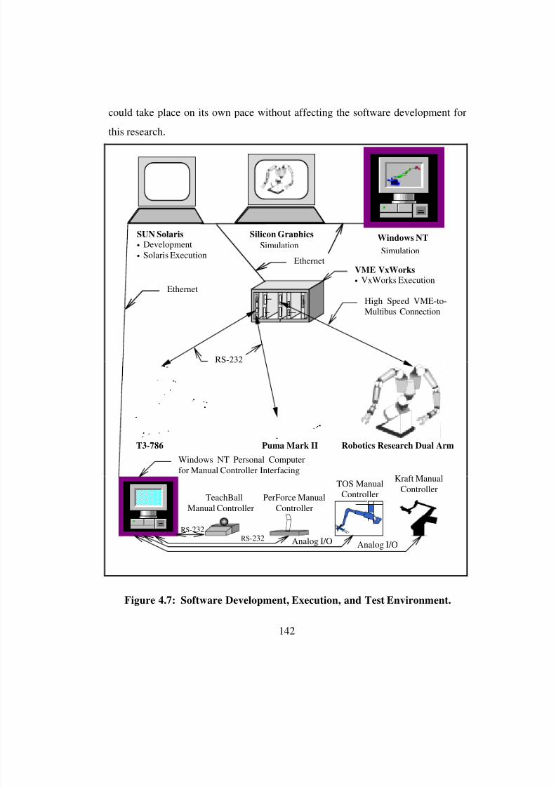
8/3/2019 Chetan Kapoor Dissertation
http://slidepdf.com/reader/full/chetan-kapoor-dissertation 166/612
142
could take place on its own pace without affecting the software development for
this research.
Figure 4.7: Software Development, Execution, and Test Environment.
Ethernet
Silicon Graphics Windows NT
VME VxWorks• VxWorks Execution
RS-232
High Speed VME-to-Multibus Connection
T3-786 Puma Mark II Robotics Research Dual Arm
Ethernet
TeachBallManual Controller
PerForce ManualController
Kraft ManualController
RS-232
Windows NT Personal Computerfor Manual Controller Interfacing
RS-232 Analog I/O Analog I/O
TOS ManualController
SUN Solaris• Development• Solaris Execution
SimulationSimulation
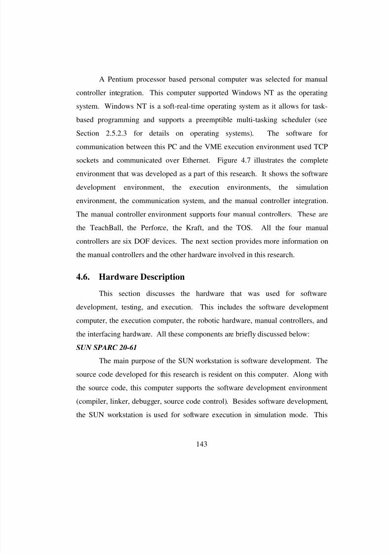
8/3/2019 Chetan Kapoor Dissertation
http://slidepdf.com/reader/full/chetan-kapoor-dissertation 167/612
143
A Pentium processor based personal computer was selected for manual
controller integration. This computer supported Windows NT as the operating
system. Windows NT is a soft-real-time operating system as it allows for task-
based programming and supports a preemptible multi-tasking scheduler (see
Section 2.5.2.3 for details on operating systems). The software for
communication between this PC and the VME execution environment used TCP
sockets and communicated over Ethernet. Figure 4.7 illustrates the complete
environment that was developed as a part of this research. It shows the software
development environment, the execution environments, the simulation
environment, the communication system, and the manual controller integration.
The manual controller environment supports four manual controllers. These are
the TeachBall, the Perforce, the Kraft, and the TOS. All the four manual
controllers are six DOF devices. The next section provides more information on
the manual controllers and the other hardware involved in this research.
4.6. Hardware Description
This section discusses the hardware that was used for software
development, testing, and execution. This includes the software development
computer, the execution computer, the robotic hardware, manual controllers, and
the interfacing hardware. All these components are briefly discussed below:
SUN SPARC 20-61
The main purpose of the SUN workstation is software development. The
source code developed for this research is resident on this computer. Along with
the source code, this computer supports the software development environment
(compiler, linker, debugger, source code control). Besides software development,
the SUN workstation is used for software execution in simulation mode. This
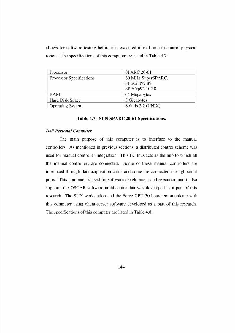
8/3/2019 Chetan Kapoor Dissertation
http://slidepdf.com/reader/full/chetan-kapoor-dissertation 168/612
144
allows for software testing before it is executed in real-time to control physical
robots. The specifications of this computer are listed in Table 4.7.
Dell Personal Computer
The main purpose of this computer is to interface to the manual
controllers. As mentioned in previous sections, a distributed control scheme was
used for manual controller integration. This PC thus acts as the hub to which all
the manual controllers are connected. Some of these manual controllers are
interfaced through data-acquisition cards and some are connected through serial
ports. This computer is used for software development and execution and it also
supports the OSCAR software architecture that was developed as a part of this
research. The SUN workstation and the Force CPU 30 board communicate with
this computer using client-server software developed as a part of this research.
The specifications of this computer are listed in Table 4.8.
Processor SPARC 20-61
Processor Specifications 60 MHz SuperSPARC.SPECint92 89
SPECfp92 102.8
RAM 64 Megabytes
Hard Disk Space 3 Gigabytes
Operating System Solaris 2.2 (UNIX)
Table 4.7: SUN SPARC 20-61 Specifications.
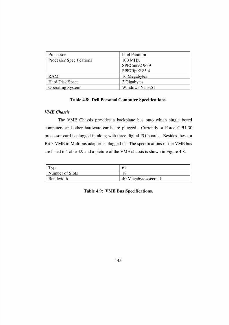
8/3/2019 Chetan Kapoor Dissertation
http://slidepdf.com/reader/full/chetan-kapoor-dissertation 169/612
145
VME ChassisThe VME Chassis provides a backplane bus onto which single board
computers and other hardware cards are plugged. Currently, a Force CPU 30
processor card is plugged in along with three digital I/O boards. Besides these, a
Bit 3 VME to Multibus adapter is plugged in. The specifications of the VME bus
are listed in Table 4.9 and a picture of the VME chassis is shown in Figure 4.8.
Processor Intel PentiumProcessor Specifications 100 MHz.SPECint92 96.9
SPECfp92 85.4
RAM 16 Megabytes
Hard Disk Space 2 Gigabytes
Operating System Windows NT 3.51
Table 4.8: Dell Personal Computer Specifications.
Type 6U
Number of Slots 18
Bandwidth 40 Megabytes/second
Table 4.9: VME Bus Specifications.
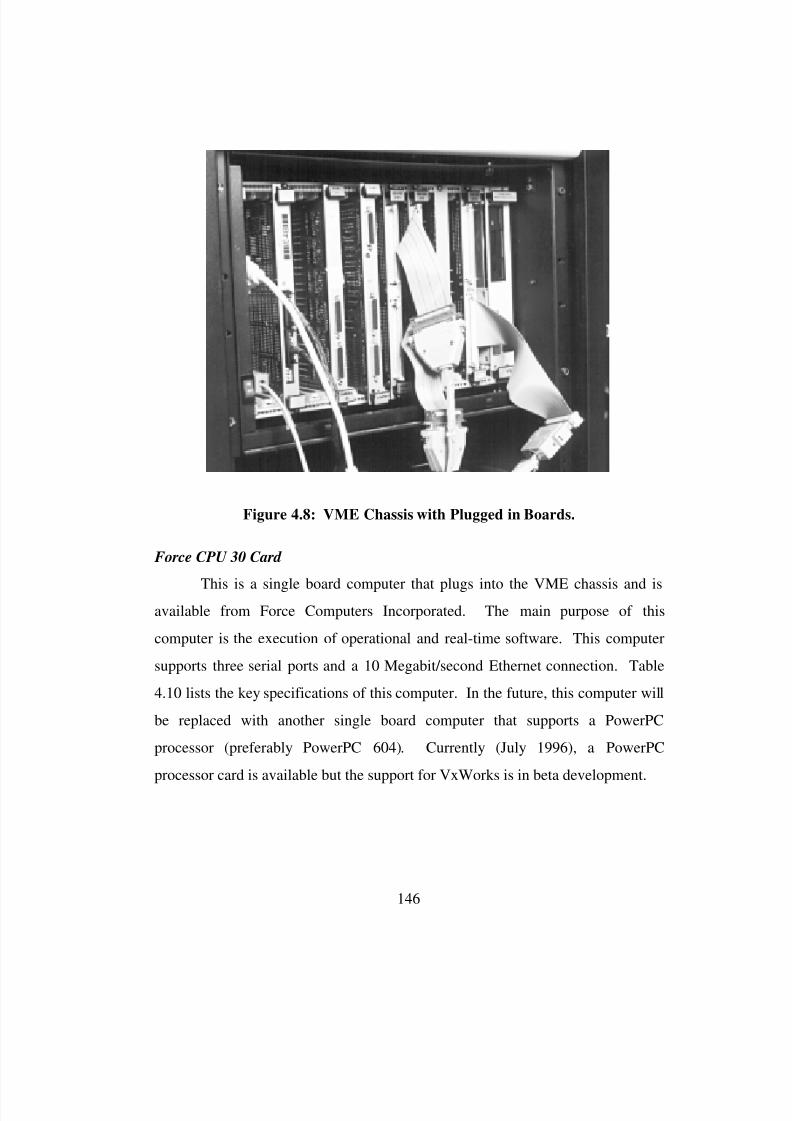
8/3/2019 Chetan Kapoor Dissertation
http://slidepdf.com/reader/full/chetan-kapoor-dissertation 170/612
146
Figure 4.8: VME Chassis with Plugged in Boards.
Force CPU 30 Card
This is a single board computer that plugs into the VME chassis and isavailable from Force Computers Incorporated. The main purpose of this
computer is the execution of operational and real-time software. This computer
supports three serial ports and a 10 Megabit/second Ethernet connection. Table
4.10 lists the key specifications of this computer. In the future, this computer will
be replaced with another single board computer that supports a PowerPC
processor (preferably PowerPC 604). Currently (July 1996), a PowerPC
processor card is available but the support for VxWorks is in beta development.
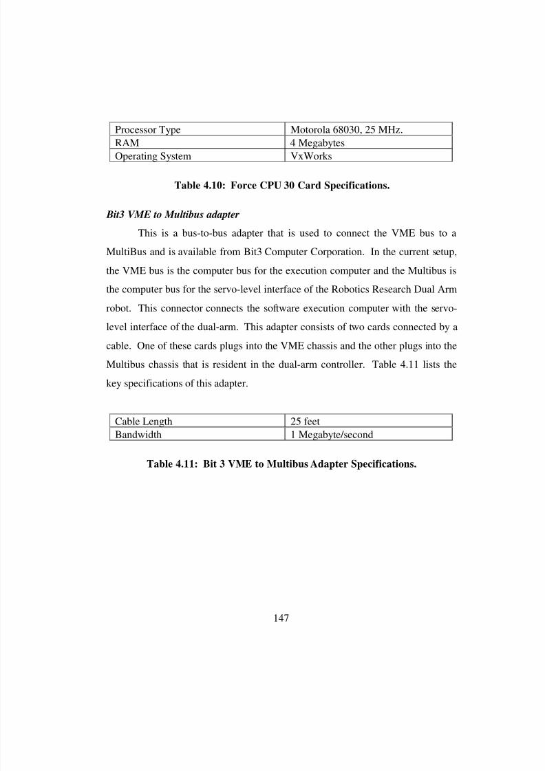
8/3/2019 Chetan Kapoor Dissertation
http://slidepdf.com/reader/full/chetan-kapoor-dissertation 171/612
147
Bit3 VME to Multibus adapter
This is a bus-to-bus adapter that is used to connect the VME bus to a
MultiBus and is available from Bit3 Computer Corporation. In the current setup,
the VME bus is the computer bus for the execution computer and the Multibus is
the computer bus for the servo-level interface of the Robotics Research Dual Arm
robot. This connector connects the software execution computer with the servo-
level interface of the dual-arm. This adapter consists of two cards connected by a
cable. One of these cards plugs into the VME chassis and the other plugs into the
Multibus chassis that is resident in the dual-arm controller. Table 4.11 lists the
key specifications of this adapter.
Processor Type Motorola 68030, 25 MHz.RAM 4 Megabytes
Operating System VxWorks
Table 4.10: Force CPU 30 Card Specifications.
Cable Length 25 feet
Bandwidth 1 Megabyte/second
Table 4.11: Bit 3 VME to Multibus Adapter Specifications.
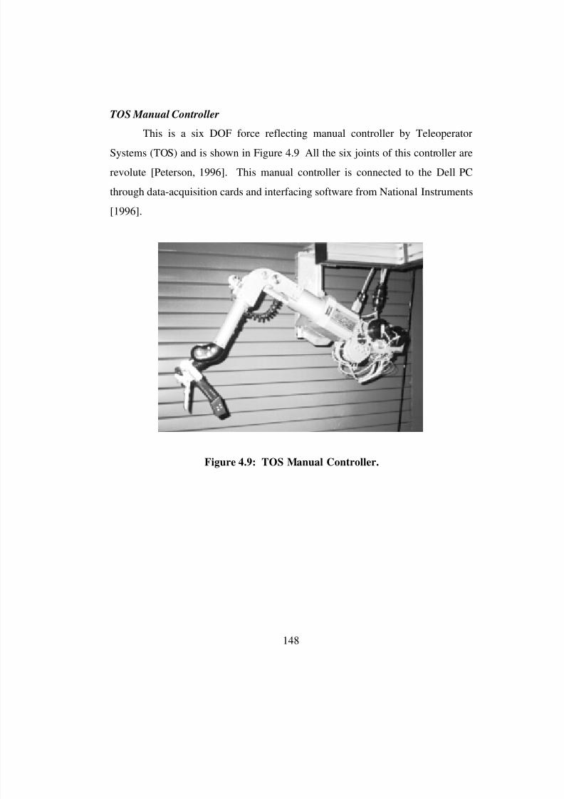
8/3/2019 Chetan Kapoor Dissertation
http://slidepdf.com/reader/full/chetan-kapoor-dissertation 172/612
148
TOS Manual Controller
This is a six DOF force reflecting manual controller by Teleoperator
Systems (TOS) and is shown in Figure 4.9 All the six joints of this controller are
revolute [Peterson, 1996]. This manual controller is connected to the Dell PC
through data-acquisition cards and interfacing software from National Instruments
[1996].
Figure 4.9: TOS Manual Controller.

8/3/2019 Chetan Kapoor Dissertation
http://slidepdf.com/reader/full/chetan-kapoor-dissertation 173/612
149
Kraft Manual Controller
This is a six DOF force reflecting manual controller from Kraft and is
shown in Figure 4.10. All six joints of this controller are revolute. The last joint
is not actuated and thus does not offer force reflection [Peterson, 1996]. This
manual controller is interfaced to the Dell PC via National Instruments data
acquisition hardware and software.
Figure 4.10: Kraft Manual Controller.
8/3/2019 Chetan Kapoor Dissertation
http://slidepdf.com/reader/full/chetan-kapoor-dissertation 174/612
150
NASA PerForce Manual Controller
This is a six DOF force reflecting manual controller from Cybernet
Systems Corporation. The first three joints of this controller are prismatic and are
used for position information. The last three joints are revolute and are used for
orientation control. This controller uses two serial ports to connect to the Dell
PC. One serial port is used to output position data and the other is used to read
the forces. Figure 4.11 shows this controller.
Figure 4.11: NASA Perforce Manual Controller.
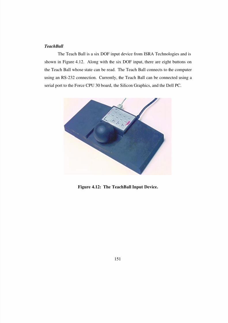
8/3/2019 Chetan Kapoor Dissertation
http://slidepdf.com/reader/full/chetan-kapoor-dissertation 175/612
151
TeachBall
The Teach Ball is a six DOF input device from ISRA Technologies and is
shown in Figure 4.12. Along with the six DOF input, there are eight buttons on
the Teach Ball whose state can be read. The Teach Ball connects to the computer
using an RS-232 connection. Currently, the Teach Ball can be connected using a
serial port to the Force CPU 30 board, the Silicon Graphics, and the Dell PC.
Figure 4.12: The TeachBall Input Device.
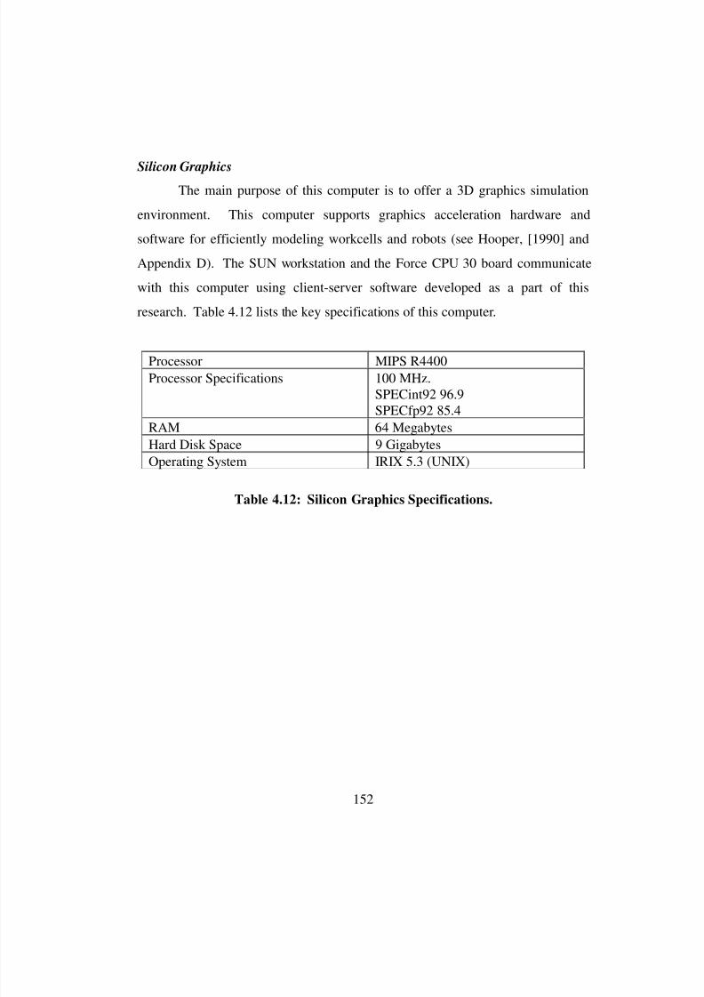
8/3/2019 Chetan Kapoor Dissertation
http://slidepdf.com/reader/full/chetan-kapoor-dissertation 176/612
152
Silicon Graphics
The main purpose of this computer is to offer a 3D graphics simulation
environment. This computer supports graphics acceleration hardware and
software for efficiently modeling workcells and robots (see Hooper, [1990] and
Appendix D). The SUN workstation and the Force CPU 30 board communicate
with this computer using client-server software developed as a part of this
research. Table 4.12 lists the key specifications of this computer.
Processor MIPS R4400
Processor Specifications 100 MHz.SPECint92 96.9SPECfp92 85.4
RAM 64 Megabytes
Hard Disk Space 9 Gigabytes
Operating System IRIX 5.3 (UNIX)
Table 4.12: Silicon Graphics Specifications.
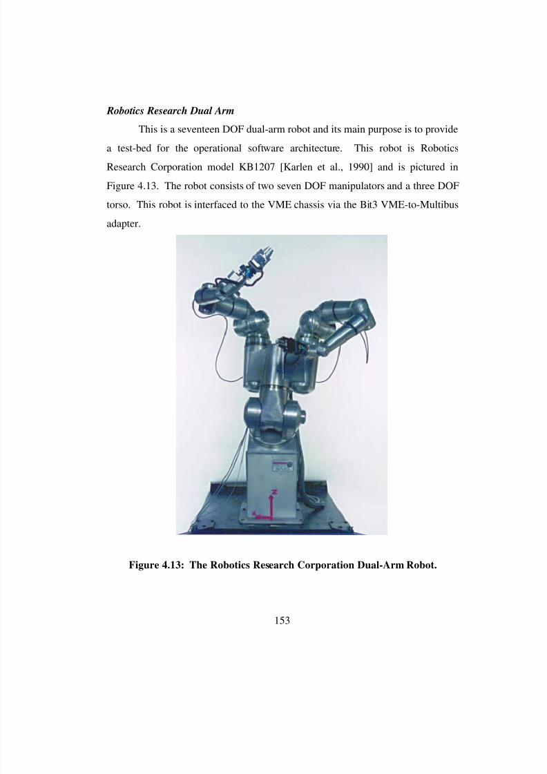
8/3/2019 Chetan Kapoor Dissertation
http://slidepdf.com/reader/full/chetan-kapoor-dissertation 177/612
153
Robotics Research Dual Arm
This is a seventeen DOF dual-arm robot and its main purpose is to provide
a test-bed for the operational software architecture. This robot is Robotics
Research Corporation model KB1207 [Karlen et al., 1990] and is pictured in
Figure 4.13. The robot consists of two seven DOF manipulators and a three DOF
torso. This robot is interfaced to the VME chassis via the Bit3 VME-to-Multibus
adapter.
Figure 4.13: The Robotics Research Corporation Dual-Arm Robot.
8/3/2019 Chetan Kapoor Dissertation
http://slidepdf.com/reader/full/chetan-kapoor-dissertation 178/612
154
Puma Mark II 500 Series Robot
This is a six DOF industrial robot from Unimation Robotics [Unimation
Robotics, 1983]. The main purpose of this robot is for testing the applicability of
the software architecture being developed as a part of this research. This robot is
connected to the real-time software execution environment through an RS-232
link using a serial port on the Force CPU-30 computer.
Cincinnati T3-786 Robot
This is a six DOF industrial robot from Cincinnati Milacron Incorporated
[ABB Robotics Incorporated]. The main purpose of this robot is for testing the
applicability of the software architecture being developed as a part of this
research. Soon this robot will be integrated into a manufacturing cell
environment. The VME chassis will be connected to this robot through an RS-
232 serial port interface.
4.7. Organizational and Managerial Issues
The success of large-scale software systems that involve more than one
developer depends largely on the organization and management of the project. As
mentioned earlier, it was the purpose of this research to develop operational
software components for advanced robotics. These components should promote
reuse via generality and extensibility. From experience it was known that these
components would not fulfill their goal of reusability unless they were made
available to software developers in a consistent and organized fashion. Thus, it
was necessary to develop some software development guidelines and to organize
the source code consistently.
The software development guidelines assist the developer in following
consistent coding conventions. For example, it is suggested in the guidelines that
any C++ class that is developed for this research should have ‘RR’ appended to its
8/3/2019 Chetan Kapoor Dissertation
http://slidepdf.com/reader/full/chetan-kapoor-dissertation 179/612
155
name. Thus, the Matrix class is called ‘RRMatrix.’ The reader should refer to
Appendix A for more details on the software development guidelines. An
advantage of following these guidelines is that the source code has a uniform look
and feel. Also, the effect of individual idiosyncrasies is minimized.
Once a uniform set of guidelines for code development was in place, the
next step was the organization of the source code. For this research, the source
code was organized based on the domains the code was addressing. Essentially,
related source code was placed in a single directory and there was a separate
directory for each domain. Details of this breakdown are given in Section C.3.3.
4.8. Summary
This chapter addressed the issues involved in the selection of the
development, execution and test environment for the operational software
components being developed for this research. The process for selecting the
development and execution environment relied on independent selection of
individual sub-systems and then iteration to achieve a practical balance. Finally, a
cross-development environment was selected that relied on a SUN workstation as
the host computer on which software is developed. C++ and object-oriented
design were chosen as the programming language and the design methodology
respectively. The selection of the execution environment was primarily driven by
the computation speed of the hardware, the extensibility of the hardware, and the
availability of a real-time operating system. It was seen that a VME-based
computer with a PowerPC processor and VxWorks as the real-time operating
system was the best candidate. After the selection of the development and
execution environment it was necessary to develop the test environment. As the
VME-based execution environment was a single-user environment, changes were
made to the development environment that allowed for code to be compiled for
8/3/2019 Chetan Kapoor Dissertation
http://slidepdf.com/reader/full/chetan-kapoor-dissertation 180/612
156
execution on the development computer (SUN workstation) itself. Using this
setup, source code development and execution could simultaneously be
undertaken by more than one user. Additionally, simulation support was added to
the execution environment. Now the user could divert the output of their control
programs to a simulation instead of a physical robot. This approach was essential
for improving the efficiency of software development. Also, various physical
robots were made available for final testing of the control programs developed by
the user. Manual controller integration software and hardware was also provided
as a part of this environment. This allowed for rapid testing of different manual
controllers and provided a means of teleoperating physical robots or simulations.
The ultimate application of this research will be to manufacturing cell
control. The distributed environment shown in Figure 4.7 will be modified to
support full cell control. However, the basic principles of object-oriented design,
distributed control, and real-time control will still apply. A preliminary layout of
the manufacturing cell control environment is shown in Figure 4.14.
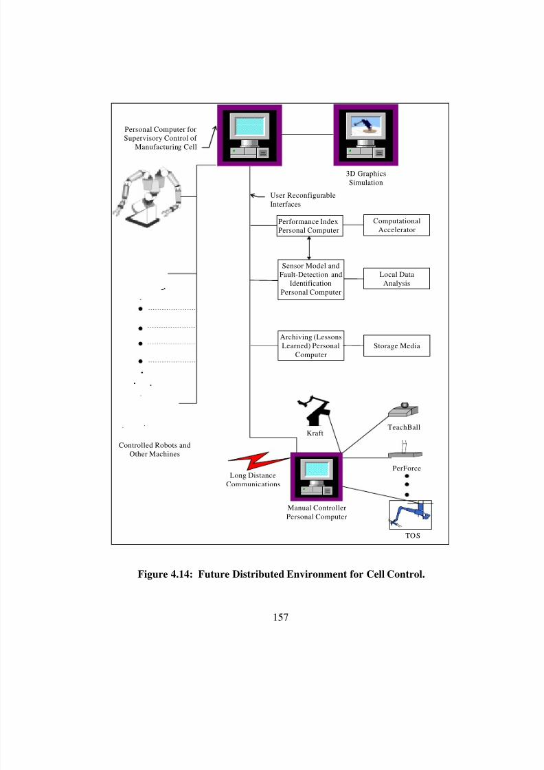
8/3/2019 Chetan Kapoor Dissertation
http://slidepdf.com/reader/full/chetan-kapoor-dissertation 181/612
157
3D Graphics
Simulation
Manual Controller
Personal Computer
Long Distance
Communications
Performance IndexPersonal Computer
KraftTeachBall
ComputationalAccelerator
PerForce
Sensor Model andFault-Detection and
Identification
Personal Computer
Local Data
Analysis
Archiving (LessonsLearned) Personal
ComputerStorage Media
User Reconfigurable
Interfaces
Personal Computer forSupervisory Control of
Manufacturing Cell
Controlled Robots andOther Machines
TOS
Figure 4.14: Future Distributed Environment for Cell Control.

8/3/2019 Chetan Kapoor Dissertation
http://slidepdf.com/reader/full/chetan-kapoor-dissertation 182/612
158
Chapter Five
5. Abstraction Development
5.1. Introduction
The presence of a large base of component suppliers is characteristic of a
mature industry. For example, the automobile industry is supported by a large
base of ancillary industry. Also, the personal computer hardware market has a
distinct component industry. Surprisingly, the component industry is barely
present for software (a major U.S. industry). This lack of a component industry is
even more noticeable in the arena of intelligent machine software. However, the
software component industry is growing mainly due to the popularity of object-
oriented design.
Object-oriented design allows the building of software components with
standardized interfaces and reuse capability. This reuse is achieved by generality
and extensibility. Generality refers to the ability of one system to serve, without
modification, in a large range of circumstances. An example of generality is
when the same forward kinematics component can be used for different robots.
Extensibility of a system refers to the ability of a system to be modified
easily to better meet a particular need. An example of a general and extensible
system is a personal computer (PC). A PC can be used for a wide range of
8/3/2019 Chetan Kapoor Dissertation
http://slidepdf.com/reader/full/chetan-kapoor-dissertation 183/612
159
purposes, ranging from word-processing to programming. Thus, reuse is
achieved through generality. A PC can also allow for hardware modifications
like additional memory. This is reuse through extensibility. Extensibility can be
achieved in two ways. The first, specialization, allows for the customization of an
existing component by changing, extending or even constraining based on need.
Thus, a user can extend the functionality by writing code that is combined with
the existing implementation to form a “new” implementation. This is also called
inheritance. The second means of extensibility is through containment. Using
containment, a variety of components can be grouped together to make a new
higher level component that hides the working details of the components it is
made of, thus giving it a black-box appearance. Borrowing from cognitive
science and entity-relationship information modeling, specialization and
containment are also respectively termed as IS-A and HAS-A relationships
[Coplien, 1994].
A literature review of robotic software systems showed that none of these
systems provided an architecture for generalized kinematics, dynamics, deflection
compensation, and decision making. Moreover, object-oriented design was onlyused to provide better robot programming interfaces. In addition, most of these
systems were implemented keeping in mind the scarcity of computer resources
and limited CPU power. This constraint made these systems excessively specific
and inextensible (see Chapter Two for detailed background information).
Availability of inexpensive computer power will be a key factor in the
design of future machines. Thus, it is necessary to research robotic software
systems with an awareness of the present and future state-of-the-art in computing.
Currently, advanced UNIX workstations offer 400 MFLOP performance [Lewis,
1994]. This performance level is sufficient to implement full dynamics,
kinematics, deflection modeling, and some criteria-based decision making
[Hernandez et al., 1989]. Also, the gap between personal computers and
8/3/2019 Chetan Kapoor Dissertation
http://slidepdf.com/reader/full/chetan-kapoor-dissertation 184/612
160
workstations is decreasing. A ten time increase in the performance of personal
computers by the year 2000 is predicted. This will lead to desk-top personal
computers capable of 800 million-instructions-per-second (MIPS) [Lewis, 1994].
Currently, advanced workstations and low-end super-computers offer this
performance level. This prediction for computer technology has a definite impact
on this research. With a decrease in the price-performance ratio of computer
hardware, software will be the commodity that will be more expensive than the
hardware. To warrant this high value in the software, researchers will be forced
to develop generalized algorithms using the latest in software design and
engineering methodologies: methodologies that promote reuse and extensibility.
Thus, a software environment is needed that fully exploits the
breakthroughs in computer hardware and software technology. This environment
should provide the researcher with a system built on a framework of generalized
kinematics, dynamics, deflection modeling, criteria-based decision making, and
fault-tolerance. This system should also support a 3D graphic modeling
environment that allows for visualization, demonstration, and testing. The
software for this environment should be developed using object-orientedmethodology, thus providing a path for reuse and standardization. Moreover, this
software should be equally applicable to real-time control. The user should be
able to divert the output of this software from a graphical environment to an
actual hardware environment with minimal effort. The software environment
described above has been developed as a part of this research. This software
architecture and its development environment is also collectively called in this
report the Operational Software Components for Advanced Robotics (OSCAR).
The literature reviewed for this research clearly showed that object-
oriented design was an efficient means of developing reusable software
components for intelligent machines. These components have a black-box
appearance and abstract the functionality of the software thus allowing an
8/3/2019 Chetan Kapoor Dissertation
http://slidepdf.com/reader/full/chetan-kapoor-dissertation 185/612
161
application developer to design software at a higher level of abstraction. This
allows for rapid-prototyping.
There are three major steps that are involved in designing object-oriented
software components. The first step is the analysis of the problem domain. This
usually leads to the breakdown of the domain into sub-domains. The net result of
the analysis phase is a set of entities and the relationships between the entities.
The functionality of these entities is also defined in this phase. The next step is
the software design. Decisions are made in the design phase based on the
execution environment, the programming language, and the operational
constraints. The entities identified in the analysis phase take the form of classes
and objects in the design phase. The third step is the implementation of the
software. These three steps are iterative and there is communication back-and-
forth among the three phases. The next section describes these three phases of
object-oriented development in detail.
5.2. Abstraction Development Process
The quality of a product is most influenced by its architecture and design.This is not a new phenomenon and has been addressed by designers through out
engineering history [Pahl and Beitz, 1988]. The architecture and design of
products is specified in the earlier stages of product development. This puts in
place the long-term sustaining structure of the product. A well designed structure
will endure well and accommodate evolution gracefully. The object-oriented
paradigm was discussed in Chapter Two. This paradigm is well-suited to
structuring a wide variety of complex systems and the key to successful
application of this paradigm is an understanding of what things make good
classes, objects, and member functions, and what things do not. The following
sections describe the three major steps that were followed for abstraction
development for this research. These are analysis, design, and implementation. It
8/3/2019 Chetan Kapoor Dissertation
http://slidepdf.com/reader/full/chetan-kapoor-dissertation 186/612
162
should be noted that the design technique described is not formal; most
techniques in practice are not. The human mind is the best “tool” to support these
techniques. [Coplien, 1994]
5.2.1. Analysis
Mellor et al. [1988] state that “the purpose of analysis is to provide a
description of a problem. The description must be complete, consistent, readable,
and reviewable by diverse interested parties [and] testable against reality.” In
essence, the purpose of analysis is to provide a model of a system’s behavior.
Thus, an analysis should yield a description of what a system does and not how it
does it. In object-oriented terminology, this means identifying the entities that
comprise the system. Broadly, the analysis process can be broken down into the
following steps [Coplien, 1994]:
Identify the entities that comprise the application domain. Entities can often
be selected by picking the nouns from the problem statement provided by end
users. These may be resources, events, or other well-defined “crisp” areas of
specialization or expertise. For example, if the user expects a software for traffic-
light control, a traffic-light can be made an entity. The selected entities generally
map to classes or objects in the design and implementation stage. Some rules of
thumb can be used to select entities and gauge their quality:
⇒ It should be easy to identify and name the behaviors of an entity.
⇒ The entity’s behaviors should relate to each other and to the entity in an
intuitively satisfying way.
⇒ The size of the abstraction should be appropriate (see Coplien [1994] for
details).
⇒ If two implementations of an entity are not possible, a broader abstraction is
probably needed. [Coplien, 1994]
8/3/2019 Chetan Kapoor Dissertation
http://slidepdf.com/reader/full/chetan-kapoor-dissertation 187/612
163
Identify the behaviors of the entities. This is the second step in the analysis
process for object-oriented software development and it involves identifying the
responsibilities of the entities in the application. These responsibilities are
characterized by the services and behavior of the class. “Good” behaviors are
crisp, clear, and concise. Again, the key here is to have a minimal possible
interface that provides the maximum possible functionality and is broad enough
to serve a wide variety of systems within the application domain.
Identify the relationships between various entities. Like real-world entities,
software entities also have relationships. These relationships can be mapped
directly onto corresponding C++ class and object structures. Some of the
relationships that can be possible are described below:
The IS-A Relationship. IS-A is a specialization relationship between classes.
For example, a four-by-four homogenous transformation matrix is a type of
matrix. The IS-A relationship maps to an inheritance hierarchy in the
implementation phase. Here the four-by-four homogenous transformation
matrix class will be derived from the matrix class, and thus would inherit its
functionality. [Coplien, 1994]The HAS-A Relationship. A HAS-A relationship connotes containment.
This relationship can be used to express the containment of a class within
another class, or of an object (instance of a class) between a class, or of an
object within an object. For example, in the case of a software for zoo
management, in all probability there will be a zoo and an animal entity.
Additionally, the zoo entity will have a set of animal entities inside it. For
example, “the zoo has a Zebra.” [Coplien, 1994]
The USES-A Relationship. The USES-A relationship is present if the
function interface of a class takes an instance of some other class (which it
uses) as a parameter. USES-A relationships are used when two classes need
to collaborate to accomplish the task. For example, consider a software
8/3/2019 Chetan Kapoor Dissertation
http://slidepdf.com/reader/full/chetan-kapoor-dissertation 188/612
164
architecture for the management of an organization. Assume that there are
classes for Vice President and Department Head. In all probability the
interface for the Vice President class may have a function that takes the
Department Head as a parameter. This function may be used by the Vice
President to accomplish some joint task. In this case, the Vice President uses
the department head but does not have him. [Coplien, 1994]
Thus, in brief, the analysis phase results in the identification of key
components that make up the software systems. The relationships between the
various components and their interface is also defined. The next section describes
the second step in object-oriented program development.
5.2.2. Design
The design phase leads to the specification of classes and objects. The
entities that were defined in the analysis phase are good candidates for this. Some
of the entities map onto objects in the running program and generalization of
some entities maps onto classes. At this point names are given to classes and
these names should reflect the semantics of the application domain. [Coplien,
1994]
The design phase also involves defining relationships. As mentioned
before, the analysis phase identified the relationship between entities. In the
design phase these relationships are transformed into inheritance hierarchies or
containment relationships. [Coplien, 1994]
5.2.3. Implementation
The implementation phase of the object-oriented program development
involves filling in the details of the class data structures, adding internal
functionality to support overall class functionality, and writing member functions.
8/3/2019 Chetan Kapoor Dissertation
http://slidepdf.com/reader/full/chetan-kapoor-dissertation 189/612
165
Additionally, unit testing of the member functions and classes, and fine-tuning of
the system should take place during implementation.
It should be noted that analysis, design and implementation are not
sequential steps. The activities are performed in a back-and-forth order,
sometimes even in parallel, until iteration comes to a minimum and the system
converges on stability. Also, under the object paradigm, the focus is more on the
design of the pieces rather than the interactions of the pieces. Interactions are, of
course, important as they are what get the job done. However, architectural
integrity of the system comes from the structure of its interfaces: object
interfaces create structures that tend to encapsulate change well and evolve
gracefully [Coplien, 1994]. This philosophy is the same as professed by
traditional mechanical designers, that is, “design in parts” [Pahl and Beitz, 1988].
5.3. Abstraction Development
Overall, the goal of this research is to perform an analysis of the domain
of advanced robotic systems and design a software architecture that allows for
extended program development for these systems. This architecture includes thespecification of software components (classes in C++). This includes their
interface, functionality, and their relationship with other components (which
might be called modules). As mentioned earlier, a requirement of these
components is to exhibit reuse through generality and extensibility. The first step
in the development of the software components was the analysis of the problem
domain of advanced robotics. This analysis is presented below:
Analysis of The Advanced Robotics Domain
Chapter One introduced some of the constructs involved in advanced
robotic systems. These were generalized kinematics, dynamics, deflection
modeling, performance criteria, and fault-tolerance. Chapter Two discussed the
mechanical and computer hardware aspects of advanced robotics and their impact
8/3/2019 Chetan Kapoor Dissertation
http://slidepdf.com/reader/full/chetan-kapoor-dissertation 190/612
166
on the software requirements. It was concluded that to have a functional
advanced robot, operational software components had to be developed for a
manipulator in the following areas:
• geometric properties,
• compliance properties,
• dynamic properties,
• generalized inverse,
• performance criteria.
The areas outlined above provide the sub-domains of the advanced robotic
domain. An analysis had to be performed on each of these domains and key
components had to be identified. After that, software components were to be
designed, implement, and tested. However, before this was done, it was
necessary to identify other domains whose development would be necessary to
support the development of the advanced robotics sub-domains. These domains
can be divided into two categories. These are:
• domains that provide building blocks for the robotic components, and
• domains that facilitate the development and testing of the robotic components.
As far as domains that provide building blocks for robotic components are
concerned, it was observed that advanced robotics relies heavily on linear algebra
[Thomas and Tesar, 1982][Hooper, 1994]. Thus, for effectively developing
operational software components, it was necessary to develop software
abstractions that supported various linear algebra constructs. Hence, another sub-
domain of mathematical abstractions had to be established.
To facilitate development and testing of operational software components,it was necessary that some utility components be provided. For example,
software had to be provided that could be used for program timing. Besides these
domains, software components were developed that allowed for communication
8/3/2019 Chetan Kapoor Dissertation
http://slidepdf.com/reader/full/chetan-kapoor-dissertation 191/612
167
and for interfacing with external hardware. Also, domains that provided key data
structures (example, linked-list, trees, etc.; for details on data structures, see
Horowitz et al., [1993]) had to be provided to facilitate software development.
Additionally, software components had to be developed that could act as
containers for robotics-related data. For example, a software component had to
be developed that could hold the Denavit-Hartenberg [Craig, 1986] parameters of
a serial robot arm. This component acted as a container for the geometric data of
the robot.
Table 5.1 gives a listing of the sub-domains that were developed as a part
of this research. This table also gives a brief description of the domain and the
functionality supported by the software components in that domain.
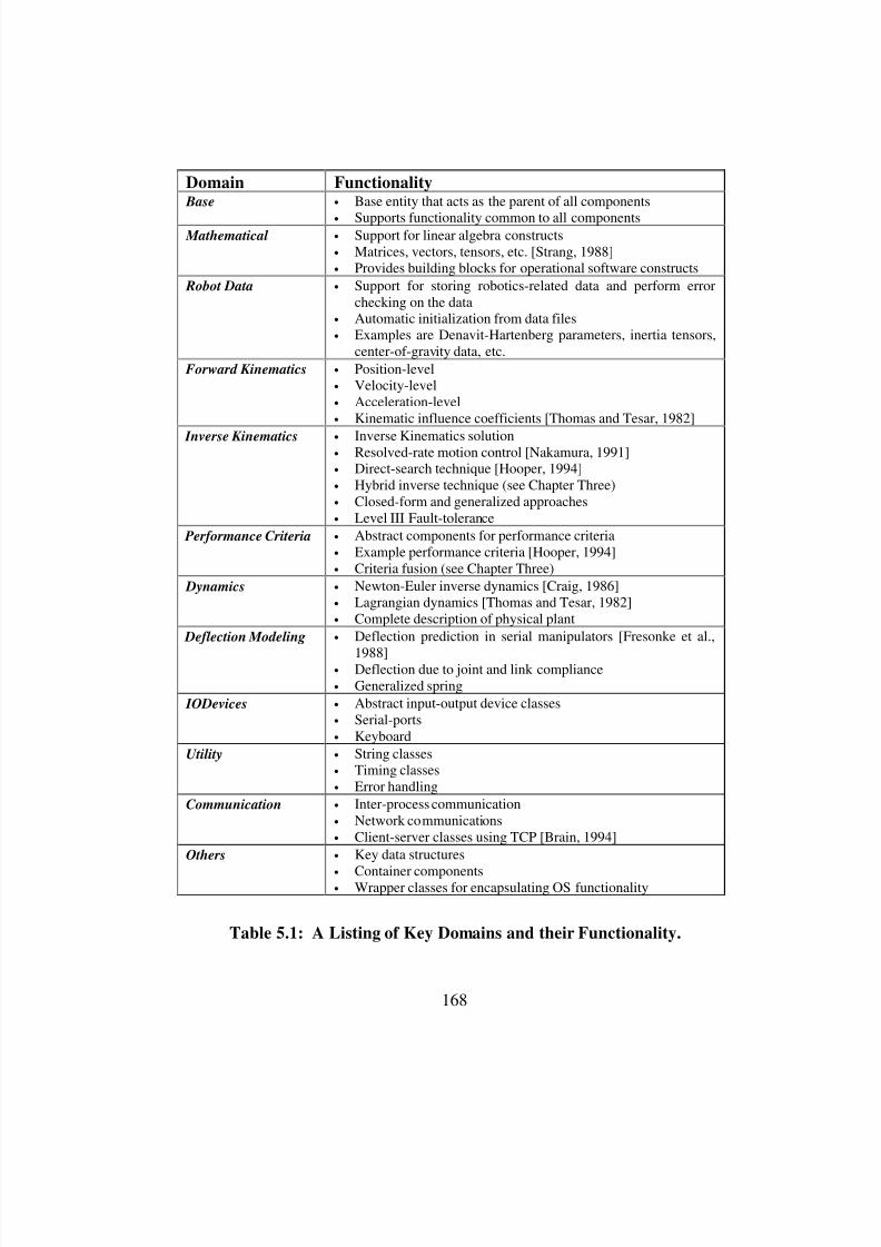
8/3/2019 Chetan Kapoor Dissertation
http://slidepdf.com/reader/full/chetan-kapoor-dissertation 192/612
168
Domain Functionality Base • Base entity that acts as the parent of all components
• Supports functionality common to all components Mathematical • Support for linear algebra constructs
• Matrices, vectors, tensors, etc. [Strang, 1988]• Provides building blocks for operational software constructs
Robot Data • Support for storing robotics-related data and perform errorchecking on the data
• Automatic initialization from data files• Examples are Denavit-Hartenberg parameters, inertia tensors,
center-of-gravity data, etc.
Forward Kinematics • Position-level• Velocity-level• Acceleration-level• Kinematic influence coefficients [Thomas and Tesar, 1982]
Inverse Kinematics • Inverse Kinematics solution• Resolved-rate motion control [Nakamura, 1991]• Direct-search technique [Hooper, 1994]• Hybrid inverse technique (see Chapter Three)• Closed-form and generalized approaches• Level III Fault-tolerance
Performance Criteria • Abstract components for performance criteria• Example performance criteria [Hooper, 1994]• Criteria fusion (see Chapter Three)
Dynamics • Newton-Euler inverse dynamics [Craig, 1986]• Lagrangian dynamics [Thomas and Tesar, 1982]• Complete description of physical plant
Deflection Modeling • Deflection prediction in serial manipulators [Fresonke et al.,
1988]• Deflection due to joint and link compliance• Generalized spring
IODevices • Abstract input-output device classes• Serial-ports• Keyboard
Utility • String classes• Timing classes• Error handling
Communication • Inter-process communication• Network communications• Client-server classes using TCP [Brain, 1994]
Others • Key data structures
• Container components• Wrapper classes for encapsulating OS functionality
Table 5.1: A Listing of Key Domains and their Functionality.
8/3/2019 Chetan Kapoor Dissertation
http://slidepdf.com/reader/full/chetan-kapoor-dissertation 193/612
169
Once the key sub-domains were selected, the next step was the analysis of
the sub-domains. This analysis led to the identification of the key entities in the
sub-domain. During the analysis phase, it also was decided that all the sub-
domains should be linked. This is because all these sub-domains belong to a
common domain of operational software. Thus, a basic entity called ‘Base’ was
created. All the other entities in this software architecture are of type Base. The
advantage of this was that functionality common to all entities could be provided
in the Base entity.
Design of The Advanced Robotics Domain
The design issues are not significant at the domain level. However, design
does achieve a significant role at the component level. That is, whenever an
analysis on a particular component is completed, design plays a key role in the
generation of implementation level specifications. As such, this section discusses
some of the design issues that were common to the design of all components in
this research. These issues are discussed below:
• All software classes developed as a part of this research had to have ‘RR’
prefixed to their name. This was done to avoid polluting the name space. Forexample, if in the future a new set of mathematical abstractions were made
available, the chances of these abstractions containing a matrix class with the
name ‘RRMatrix’ would be rare. However, if the matrix class developed as a
part of this research was named ‘Matrix,’ there would be a greater chance of a
name conflict. Other details of design and implementation guidelines are
provided in Appendix A.
• As the software developed in this research was to be applicable to real-time
control, computational efficiency was critical. However, object-oriented
program development in C++ relies on dynamic binding and operator
overloading (see Section 2.5.1.2 for details). Both dynamic binding and
operator overloading can slow down program execution. Thus, it was decided
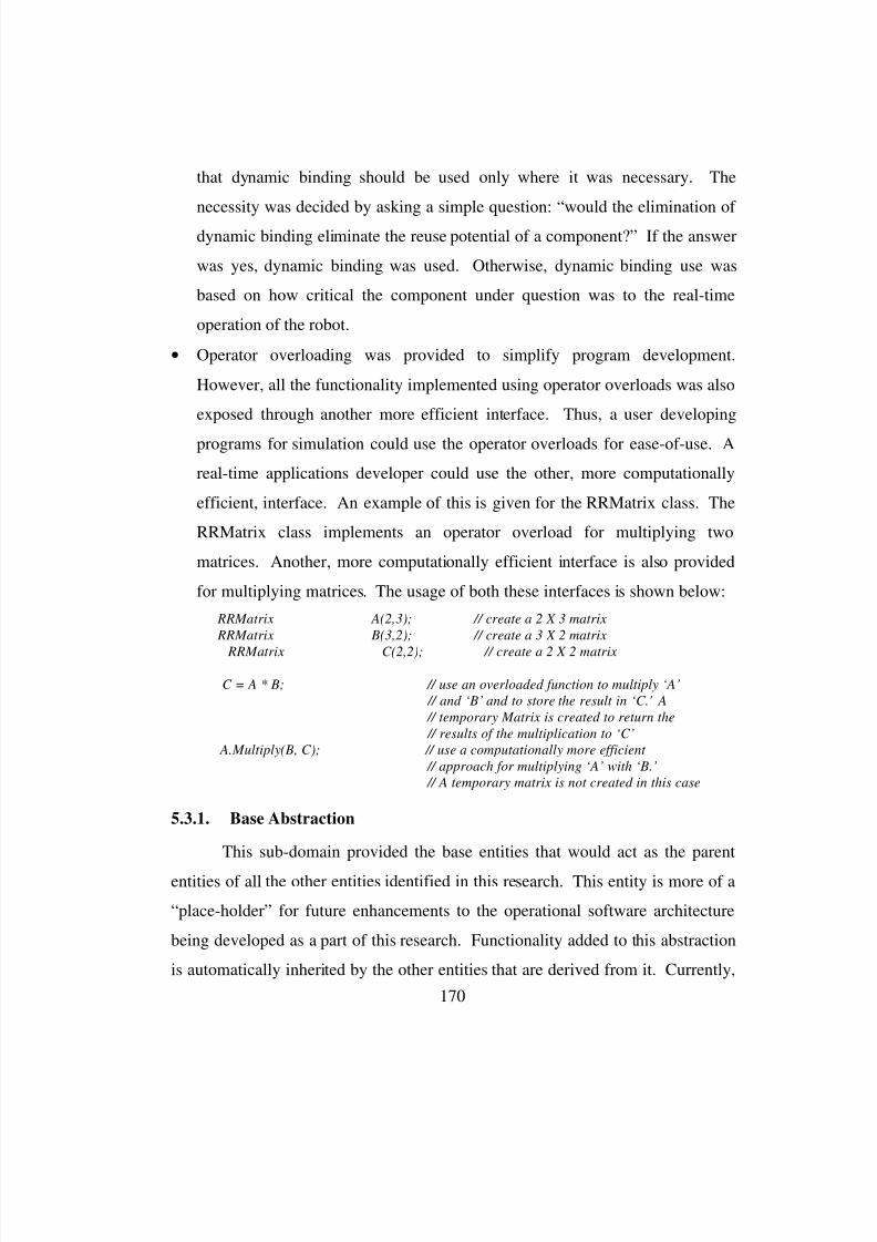
8/3/2019 Chetan Kapoor Dissertation
http://slidepdf.com/reader/full/chetan-kapoor-dissertation 194/612
170
that dynamic binding should be used only where it was necessary. The
necessity was decided by asking a simple question: “would the elimination of
dynamic binding eliminate the reuse potential of a component?” If the answer
was yes, dynamic binding was used. Otherwise, dynamic binding use was
based on how critical the component under question was to the real-time
operation of the robot.
• Operator overloading was provided to simplify program development.
However, all the functionality implemented using operator overloads was also
exposed through another more efficient interface. Thus, a user developing
programs for simulation could use the operator overloads for ease-of-use. A
real-time applications developer could use the other, more computationally
efficient, interface. An example of this is given for the RRMatrix class. The
RRMatrix class implements an operator overload for multiplying two
matrices. Another, more computationally efficient interface is also provided
for multiplying matrices. The usage of both these interfaces is shown below:
RRMatrix A(2,3); // create a 2 X 3 matrix
RRMatrix B(3,2); // create a 3 X 2 matrix
RRMatrix C(2,2); // create a 2 X 2 matrix
C = A * B; // use an overloaded function to multiply ‘A’
// and ‘B’ and to store the result in ‘C.' A
// temporary Matrix is created to return the
// results of the multiplication to ‘C’
A.Multiply(B, C); // use a computationally more efficient
// approach for multiplying ‘A’ with ‘B.’
// A temporary matrix is not created in this case
5.3.1. Base Abstraction
This sub-domain provided the base entities that would act as the parent
entities of all the other entities identified in this research. This entity is more of a
“place-holder” for future enhancements to the operational software architecture
being developed as a part of this research. Functionality added to this abstraction
is automatically inherited by the other entities that are derived from it. Currently,
8/3/2019 Chetan Kapoor Dissertation
http://slidepdf.com/reader/full/chetan-kapoor-dissertation 195/612
171
the key attribute of this abstraction is its name. Functionality is provided to
access this name and change it. This abstraction is implemented as a C++ class
and is appropriately named ‘RRBase.’ The interface for the RRBase class is
outlined in Section B.1.1.
5.3.2. Mathematical Abstractions
The key use of mathematical abstractions was to provide building blocks
for developing the operational software components. A review of robotic
literature provided a basis for the development of mathematical abstractions
[Nakamura, 1991][Thomas and Tesar, 1982]. The following requirements were
gathered from the literature review.
• Vectors, matrices, and tensors are an efficient means of managing data in
kinematics, dynamics, and deflection modeling [Thomas and Tesar, 1986].
• Homogenous transformation matrices are extensively used to express spatial
relationships in kinematics.
• Different conventions can be used to express spatial orientations. These are,
fixed-angle representations and Euler-angle representations [Craig, 1986].• Various linear algebra constructs like matrix inversion, factorization, singular
value decomposition, vector inner and cross products, etc., are essential for
operational software development.
Considering the requirements given above, the mathematical abstraction
sub-domain was further divided into the following software components. These
are listed in Table 5.2 and brief descriptions are also given. The following sub-
sections discuss the analysis and design issues faced in the development of the
software components listed in Table 5.2.
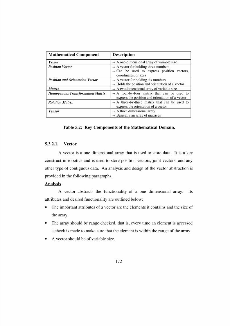
8/3/2019 Chetan Kapoor Dissertation
http://slidepdf.com/reader/full/chetan-kapoor-dissertation 196/612
172
5.3.2.1. Vector
A vector is a one dimensional array that is used to store data. It is a key
construct in robotics and is used to store position vectors, joint vectors, and any
other type of contiguous data. An analysis and design of the vector abstraction is
provided in the following paragraphs.
Analysis
A vector abstracts the functionality of a one dimensional array. Its
attributes and desired functionality are outlined below:
• The important attributes of a vector are the elements it contains and the size of
the array.
• The array should be range checked, that is, every time an element is accessed
a check is made to make sure that the element is within the range of the array.
• A vector should be of variable size.
Mathematical Component Description
Vector ⇒ A one-dimensional array of variable size
Position Vector ⇒ A vector for holding three numbers⇒ Can be used to express position vectors,
coordinates, or axes
Position and Orientation Vector ⇒ A vector for holding six numbers⇒ Holds the position and orientation of a vector
Matrix ⇒ A two dimensional array of variable size
Homogenous Transformation Matrix ⇒ A four-by-four matrix that can be used toexpress the position and orientation of a vector
Rotation Matrix ⇒ A three-by-three matrix that can be used toexpress the orientation of a vector
Tensor ⇒ A three dimensional array⇒ Basically an array of matrices
Table 5.2: Key Components of the Mathematical Domain.
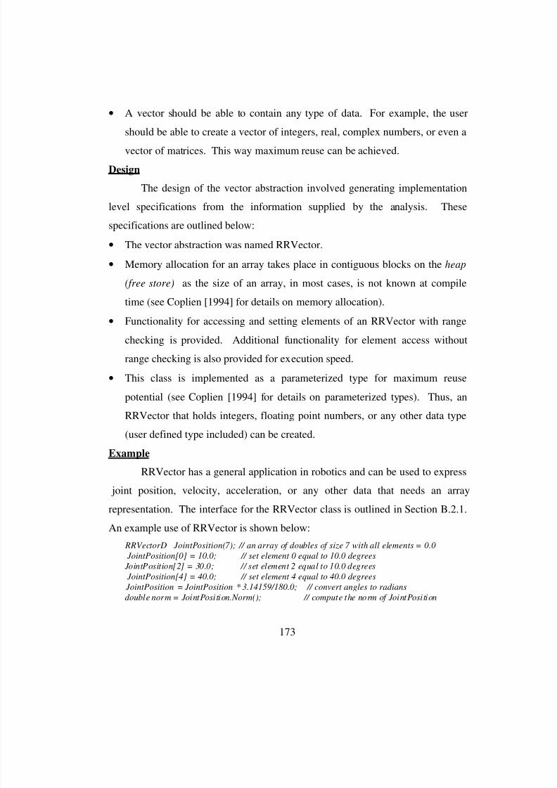
8/3/2019 Chetan Kapoor Dissertation
http://slidepdf.com/reader/full/chetan-kapoor-dissertation 197/612
173
• A vector should be able to contain any type of data. For example, the user
should be able to create a vector of integers, real, complex numbers, or even a
vector of matrices. This way maximum reuse can be achieved.
Design
The design of the vector abstraction involved generating implementation
level specifications from the information supplied by the analysis. These
specifications are outlined below:
• The vector abstraction was named RRVector.
• Memory allocation for an array takes place in contiguous blocks on the heap
(free store) as the size of an array, in most cases, is not known at compile
time (see Coplien [1994] for details on memory allocation).
• Functionality for accessing and setting elements of an RRVector with range
checking is provided. Additional functionality for element access without
range checking is also provided for execution speed.
• This class is implemented as a parameterized type for maximum reuse
potential (see Coplien [1994] for details on parameterized types). Thus, an
RRVector that holds integers, floating point numbers, or any other data type
(user defined type included) can be created.
Example
RRVector has a general application in robotics and can be used to express
joint position, velocity, acceleration, or any other data that needs an array
representation. The interface for the RRVector class is outlined in Section B.2.1.
An example use of RRVector is shown below:
RRVectorD JointPosition(7); // an array of doubles of size 7 with all elements = 0.0
JointPosition[0] = 10.0; // set element 0 equal to 10.0 degrees
JointPosition[2] = 30.0; // set element 2 equal to 10.0 degrees
JointPosition[4] = 40.0; // set element 4 equal to 40.0 degrees
JointPosition = JointPosition * 3.14159/180.0; // convert angles to radians
double norm = JointPosition.Norm(); // compute the norm of JointPosition
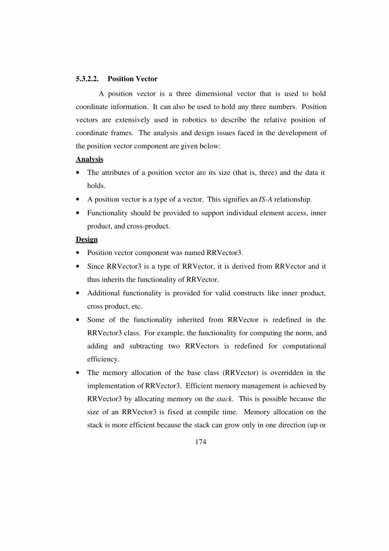
8/3/2019 Chetan Kapoor Dissertation
http://slidepdf.com/reader/full/chetan-kapoor-dissertation 198/612
174
5.3.2.2. Position Vector
A position vector is a three dimensional vector that is used to holdcoordinate information. It can also be used to hold any three numbers. Position
vectors are extensively used in robotics to describe the relative position of
coordinate frames. The analysis and design issues faced in the development of
the position vector component are given below:
Analysis
• The attributes of a position vector are its size (that is, three) and the data it
holds.
• A position vector is a type of a vector. This signifies an IS-A relationship.
• Functionality should be provided to support individual element access, inner
product, and cross-product.
Design
• Position vector component was named RRVector3.
• Since RRVector3 is a type of RRVector, it is derived from RRVector and it
thus inherits the functionality of RRVector.
• Additional functionality is provided for valid constructs like inner product,
cross product, etc.
• Some of the functionality inherited from RRVector is redefined in the
RRVector3 class. For example, the functionality for computing the norm, and
adding and subtracting two RRVectors is redefined for computational
efficiency.
• The memory allocation of the base class (RRVector) is overridden in the
implementation of RRVector3. Efficient memory management is achieved by
RRVector3 by allocating memory on the stack . This is possible because the
size of an RRVector3 is fixed at compile time. Memory allocation on the
stack is more efficient because the stack can grow only in one direction (up or
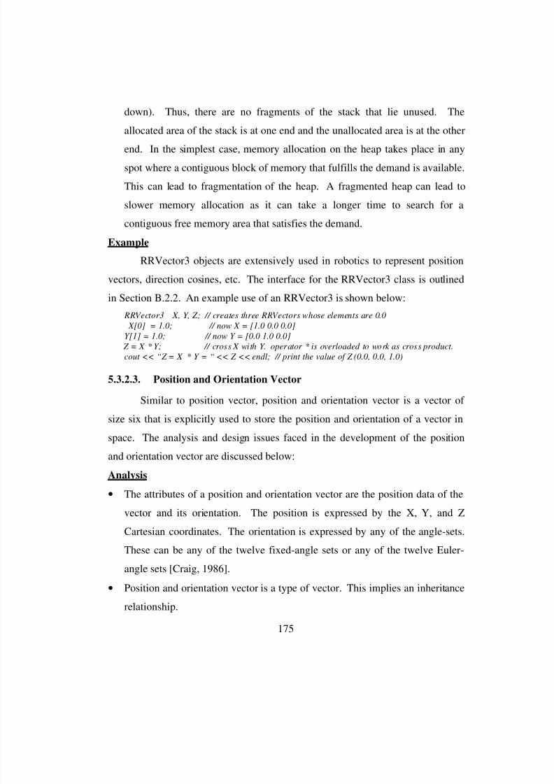
8/3/2019 Chetan Kapoor Dissertation
http://slidepdf.com/reader/full/chetan-kapoor-dissertation 199/612
175
down). Thus, there are no fragments of the stack that lie unused. The
allocated area of the stack is at one end and the unallocated area is at the other
end. In the simplest case, memory allocation on the heap takes place in any
spot where a contiguous block of memory that fulfills the demand is available.
This can lead to fragmentation of the heap. A fragmented heap can lead to
slower memory allocation as it can take a longer time to search for a
contiguous free memory area that satisfies the demand.
Example
RRVector3 objects are extensively used in robotics to represent position
vectors, direction cosines, etc. The interface for the RRVector3 class is outlined
in Section B.2.2. An example use of an RRVector3 is shown below:
RRVector3 X, Y, Z; // creates three RRVectors whose elements are 0.0
X[0] = 1.0; // now X = [1.0 0.0 0.0]
Y[1] = 1.0; // now Y = [0.0 1.0 0.0]
Z = X * Y; // cross X with Y. operator * is overloaded to work as cross product.
cout << “Z = X * Y = “ << Z << endl; // print the value of Z (0.0, 0.0, 1.0)
5.3.2.3. Position and Orientation Vector
Similar to position vector, position and orientation vector is a vector of
size six that is explicitly used to store the position and orientation of a vector in
space. The analysis and design issues faced in the development of the position
and orientation vector are discussed below:
Analysis
• The attributes of a position and orientation vector are the position data of the
vector and its orientation. The position is expressed by the X, Y, and Z
Cartesian coordinates. The orientation is expressed by any of the angle-sets.
These can be any of the twelve fixed-angle sets or any of the twelve Euler-
angle sets [Craig, 1986].
• Position and orientation vector is a type of vector. This implies an inheritance
relationship.
8/3/2019 Chetan Kapoor Dissertation
http://slidepdf.com/reader/full/chetan-kapoor-dissertation 200/612
176
• Functionality should be provided that allows for conversion of a position and
orientation vector into a four-by-four homogenous transformation matrix
representation.
Design
• The position and orientation vector component is given the name
RRHandPose. This was done because, under the domain of robotics, this
component was generally used to express the position and orientation of the
hand of a robot arm.
• RRHandPose was derived from RRVector as it is a type of RRVector.
• As the size of RRHandPose is fixed (size is six), RRHandPose overrides the
memory management of its parent, the RRVector. Memory allocation for
RRHandPose takes place on the stack as opposed to the heap.
• Functionality to convert an RRHandPose to an RRXform (see Section 5.3.2.5
for details on RRXform) is also provided.
Example
RRHandPose is used in robotics to represent the position and orientation
of a vector in space. By changing the angle representation (any of the Euler or
fixed angles) of the orientation, different means of controlling the end-effector
position orientations can be exercised. The example shown below creates an
RRHandPose object and specifies that the orientation be expressed in ZYZ Euler
angles. After that, the ’X’ coordinate and the Alpha and Gamma angles are set.
The next step converts the RRHandPose object into its RRXform representation.
The interface for the RRHandPose class is outlined in Section B.2.3.
RRHandPosehand(EULER_ZYZ); // create an RRHandPose vector that
// represents the Cartesian position and the
// ZYZ Euler angles
RRXform handMatrix; // create a 4 X 4 transformation matrix
hand.X() = 10.0; // set X = 10.0
hand.Y() = 5.0; // set Y = 5.0 and Z = 0.0 by default
hand.Alpha() = 0.1; // set alpha angle = 0.1 radians
hand.Gamma() = 0.2; // set Gamma = 0.2 radians. Beta = 0.0

8/3/2019 Chetan Kapoor Dissertation
http://slidepdf.com/reader/full/chetan-kapoor-dissertation 201/612
177
handMatrix = hand.ToTransform(); // convert hand into its 4 X 4 representation
5.3.2.4. Matrix
A matrix is a key linear algebra construct that is used to hold two-
dimensional data. The data held by a matrix could be integers, real numbers, or
complex numbers. The following paragraphs discuss the analysis and design
issues faced in the development of the matrix component. Finally, an example
use of this component is given.
Analysis
This software component abstracts the functionality of a matrix. A matrix
represents a two-dimensional array whose attributes are its elements and the
number of columns and rows.
The desired functionality of a matrix is listed below:
• Individual elements of the matrix should be accessible.
• Individual rows and columns should be accessible.
• Support linear algebra operations like inversion, transpose, LU
decomposition, singular value decomposition, etc. [Strang, 1988].
Design
The design of the matrix class involved generating specifications that
could be used for implementation. The design decisions and the reasons for
making them are listed below:
• RRMatrix was chosen as the name for the matrix abstraction. This name
effectively describes a matrix.
• Functionality was provided for inverting, transposing, singular value
decomposition, LU decomposition, multiplying, and adding matrices.
• Operator overloads were provided for multiplication, inversion, addition, and
subtraction. This was done for ease of use.

8/3/2019 Chetan Kapoor Dissertation
http://slidepdf.com/reader/full/chetan-kapoor-dissertation 202/612
178
• As a matrix object was supposed to store integers, reals, and complex
numbers, the matrix class was designed as a parameterized class (see Coplien
[1994] for details on parameterized types). This was done to achieve
maximum reuse.
• Memory allocation for an RRMatrix takes place in contiguous blocks on the
heap (free store) (See Coplien [1994] for details on memory management) as
the size of the matrix, in most cases, is not known at compile time. As a
matrix is a two-dimensional array, different memory layouts for the elements
of a matrix are possible. Figure 5.1 shows three of these layouts. The first
one allocates a contiguous block of memory whose length is equal to the
number of rows (NROW) multiplied by the number of columns (NCOL). For
accessing an element of this matrix, a simple calculation (see Figure 5.1, part
a) has to be performed. Figure 5.1, part b shows the second memory layout.
In this, each row of size NCOL is allocated separately and a column of
pointers of size NROW is also allocated. Elements are accessed by indexing
into the column of pointers and reaching the desired row. Then the desired
element is accessed from that row. The third scheme is similar to the first in
the way it allocates memory for the elements. To avoid calculation for
accessing an element, a column of size NROW is used. This column holds
pointers to the beginning of each row in the memory layout of the elements.
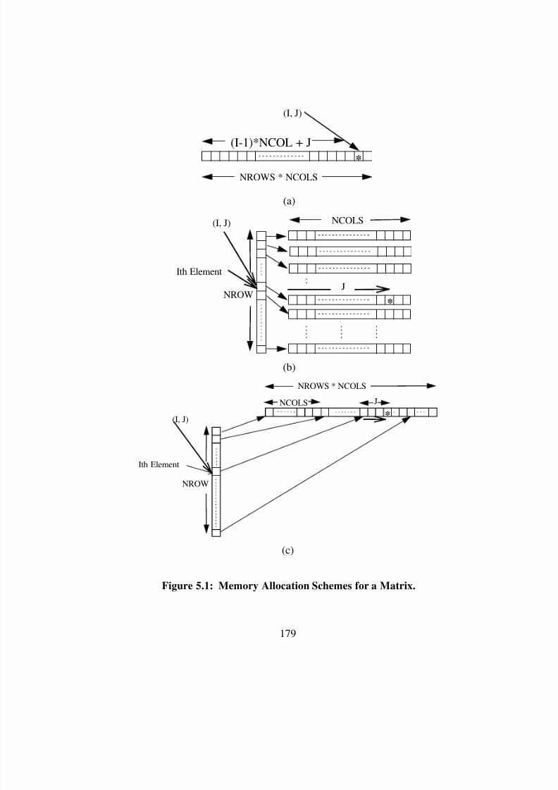
8/3/2019 Chetan Kapoor Dissertation
http://slidepdf.com/reader/full/chetan-kapoor-dissertation 203/612
179
NROWS * NCOLS
(I, J)
(I-1)*NCOL + J
*
(a)
NROW
NCOLS(I, J)
J
*
Ith Element
(b)
NROWS * NCOLS
NROW
(I, J)
NCOLS
*
J
Ith Element
(c)
Figure 5.1: Memory Allocation Schemes for a Matrix.
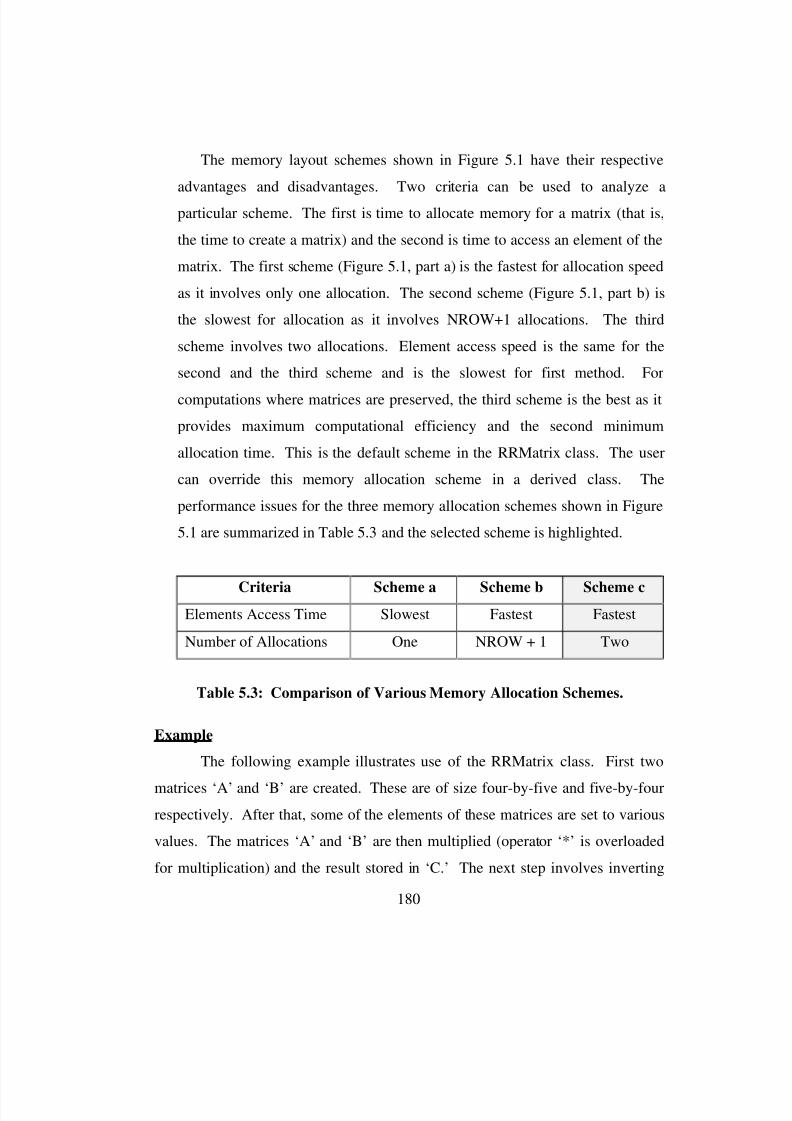
8/3/2019 Chetan Kapoor Dissertation
http://slidepdf.com/reader/full/chetan-kapoor-dissertation 204/612
180
The memory layout schemes shown in Figure 5.1 have their respective
advantages and disadvantages. Two criteria can be used to analyze a
particular scheme. The first is time to allocate memory for a matrix (that is,
the time to create a matrix) and the second is time to access an element of the
matrix. The first scheme (Figure 5.1, part a) is the fastest for allocation speed
as it involves only one allocation. The second scheme (Figure 5.1, part b) is
the slowest for allocation as it involves NROW+1 allocations. The third
scheme involves two allocations. Element access speed is the same for the
second and the third scheme and is the slowest for first method. For
computations where matrices are preserved, the third scheme is the best as it
provides maximum computational efficiency and the second minimum
allocation time. This is the default scheme in the RRMatrix class. The user
can override this memory allocation scheme in a derived class. The
performance issues for the three memory allocation schemes shown in Figure
5.1 are summarized in Table 5.3 and the selected scheme is highlighted.
Example
The following example illustrates use of the RRMatrix class. First two
matrices ‘A’ and ‘B’ are created. These are of size four-by-five and five-by-four
respectively. After that, some of the elements of these matrices are set to various
values. The matrices ‘A’ and ‘B’ are then multiplied (operator ‘*’ is overloaded
for multiplication) and the result stored in ‘C.’ The next step involves inverting
Criteria Scheme a Scheme b Scheme c
Elements Access Time Slowest Fastest Fastest
Number of Allocations One NROW + 1 Two
Table 5.3: Comparison of Various Memory Allocation Schemes.
8/3/2019 Chetan Kapoor Dissertation
http://slidepdf.com/reader/full/chetan-kapoor-dissertation 205/612
181
‘C.’ It should be noted that the operator ‘~’ is overloaded for inverting a matrix.
The interface for the RRMatrix class is outlined in Section B.2.4.
RRMatrix A(4, 5), B(5, 4); // create two matrices that contain doubles.
// By default, the matrices will be filled with zeros
A(0,0) = A(1,1) = A(3,2) = 3.0; // set some elements of A to the value 3.0
B(0,0) = B(1,2) = A(2,3) = 4.0; // set some elements of B to the value 4.0
RRMatrix C = A * B; // matrix C is created and initialized with the product
// of A and B
RRMatrix D = ~C; // matrix D is created and initialized with the inverse
// of C
5.3.2.5. Four-by-Four Homogenous Transformation Matrix
Four-by-four homogenous transformation matrices are used to represent
the relative position and orientation of two different coordinate frames. In
robotics, homogenous transformation matrices are used to represent link frames,
end-effector position and orientation, and transforms; and are used in kinematic
computations [Craig, 1986].
Analysis
The homogenous transformation matrix has the following attributes and
functionality:
• A homogenous transformation matrix is a type of matrix. This clearly
signifies an IS-A relationship. In the design phase this will map to an
inheritance relationship.
• The size of a homogenous transformation matrix is four-by-four.
• The structure of a homogenous transformation matrix consists of an upper left
three-by-three rotation matrix ( r 11 , r 12 , …, r 33 ) and the top three rows of the
last column containing the position data ( p x , p y , p z ). This is shown below:
r r r p
r r r p
r r r p
x
y
z
11 12 13
21 22 23
31 32 33
0 0 0 1
8/3/2019 Chetan Kapoor Dissertation
http://slidepdf.com/reader/full/chetan-kapoor-dissertation 206/612
182
• The user should have the ability to convert a homogenous transformation
matrix into its vector representation. The vector representation will include
the position vector ( p x , p y , p z ) and a three-by-one representation of the
orientation. The orientation representation could be any of the fixed-angle or
Euler-angle sets [Craig, 1986].
Design
The following decisions were made for the design of the four-by-four
homogenous transformation matrix data type.
• This data type was given the name RRXform.
• As RRXform is a type of RRMatrix, RRXform is derived from RRMatrix and
thus inherits all the functionality of an RRMatrix.
• Efficient memory management is achieved by RRXform by allocating
memory on the stack. This is possible because the size of an RRXform (four-
by-four) is fixed at compile time. RRXform overrides the memory allocation
of its parent class, the RRMatrix, which allocated memory on the heap.
• RRXform redefines the functionality for matrix multiplication, inversion,
transpose, addition, and subtraction. This is done purely for reasons of
computational efficiency and could have been avoided.
• RRXform also extends the functionality of an RRMatrix by providing
functionality for conversion to a six element vector that represents the ‘X,’
‘Y,’ ‘Z’ Cartesian position and the three orientation angles (RRHandPose).
Example
The following example shows the use of the RRXform data type. First an
instance of RRXform, ‘A’ is created. ‘A’, by default is an identity matrix. The
(0,3) element of A is set to value 10.0. For doing this, a method named at is used.
The method at does not perform any range checking on its arguments. Thus, the
8/3/2019 Chetan Kapoor Dissertation
http://slidepdf.com/reader/full/chetan-kapoor-dissertation 207/612
183
user has to exercise caution while using this method. Next the element (1,3) is set
to value -5.0. This method is an operator overload for ‘( )’ and performs range
checking on the indices and is thus safer to use. However, execution speed is
sacrificed for added safety and error checking. Once the elements of ‘A’ are set,
the next step is to convert ‘A’ into its vector representation. In the example
shown, ‘A’ is converted to an RRHandPose vector. Section B.2.7 outlines the
interface of the RRXform class.
RRXform A; // creates a 4 X 4 matrix that by default is an identity matrix
A.at(0,3) = 10.0; // this member function ‘at’ does not perform any range checking
A(1,3) = -5.0; // the ‘( )’ operator is overloaded and it performs range checking
RRHandPose handPose; // create a 6 X 1 hand position and orientation vector handPose = A.ToHandPose(); // convert A into its 6 X 1 vector representation
5.3.2.6. Three-by-Three Rotation Matrix
Three-by-three rotation matrices are used to represent the relative
orientation of two different coordinate frames [Craig, 1986]. The analysis and
design issues faced in the development of a three-by-three rotation matrix
component are discussed below:
Analysis
This rotation matrix has the following attributes and functionality:
• A rotation matrix is a type of matrix. This clearly signifies an IS-A
relationship. In the design phase this will map to an inheritance relationship.
• The size of a rotation matrix is three-by-three.
Design
The following decisions were made for the design of the three-by-three
rotation matrix data type.
• This data type was given the name RRRot3by3.
• As RRRot3by3 is a type of RRMatrix, RRRot3by3 is derived from RRMatrix
and thus inherits all the functionality of an RRMatrix.
8/3/2019 Chetan Kapoor Dissertation
http://slidepdf.com/reader/full/chetan-kapoor-dissertation 208/612
184
• More efficient memory management is achieved by RRRot3by3 by allocating
memory on the stack. This is possible because the size of an RRRot3by3
(three-by-three) is fixed at compile time.
• RRRot3by3 redefines the functionality for matrix multiplication, inversion,
transpose, addition, and subtraction. This is done purely for reasons of
computational efficiency and could have been avoided.
Example
The following example shows the use of the RRRot3by3 data type. First
an RRRot3by3 object ‘A’ is created. Also, two RRVector3’s, ‘B,’ and ‘C’ are
created. Then some of the elements of ‘A,’ ‘B,’ and ‘C’ are set. Finally the
rotation matrix ‘A’ is multiplied with ‘B’ and the result is stored in ‘C.’ The
interface for the RRRot3by3 class in outlined in Section B.2.8.
RRRot3by3 A; // creates a 3 X 3 matrix that by default is an identity matrix
RRVector3 B, C; // create two RRVector3 objects. By default all elements are 0.0
A.at(0,1) = 10.0; // the member function ‘at’ does not perform any range checking
A(1,1) = -5.0; // the ‘( )’ operator is overloaded and by it performs range checking
B[1] = 3.0; // set the second element of B to 3.0
A.Multiply(B, C); // multiply A with B and store the result in C. That is, C = A * B
5.3.2.7. Tensor
A tensor is a three-dimensional array. It is used in robotics software to
express kinematic influence coefficients [Thomas and Tesar, 1984]. The various
analysis and design decisions made during the development of a tensor data type
are discussed below:
Analysis
• The key attributes of a tensor are the number of rows and columns of each
plane of the tensor, the total number of planes the tensor has, and the data the
tensor holds.
• The tensor should be of variable size. That is, the user should be able to
create a tensor at run time of any desired dimension.
8/3/2019 Chetan Kapoor Dissertation
http://slidepdf.com/reader/full/chetan-kapoor-dissertation 209/612
185
• A tensor is a three dimensional matrix. In other words, a tensor is an array of
matrices, or a tensor has matrices.
• A tensor should support functionality for accessing individual elements, rows,
columns, and the matrices that comprise the tensor.
Design
• The tensor data type was given the name RRTensor.
• As a tensor is an array of matrices, an array of RRMatrix objects were
contained inside an RRTensor. Thus, RRTensor provides an example of
abstraction development through containment.
• The RRTensor provides a simplified interface for accessing the three
dimensional data inside it. Functionality is provided for accessing individual
elements and planes of the tensor.
Example
The interface for the RRTensor class is outlined in Section B.2.9 and an
example use of an RRTensor is shown below:
RRTensor A(3,4,4); // create an RRTensor of size 3 X 4 X 4. That is, a tensor
// that contains three planes of 4 X 4 matrices.
A.(0, 1,1) = 10.0; // set the (1,1) element of the plane 0 to 10.0 A.(1,2,2) = 15.0; // set the (2,2) element of the plane 1 to 15.0
A(2,3,3) = -10.0; // set the (3,3) element of the plane 2 to -10.0
A(0) = A(1) * A(2); // multiply plane 1 with plane 2 and store the result in plane 0
5.3.2.8. Summary of Mathematical Components
The previous sections discussed the analysis and design details of the
various software components that were developed as a part of the mathematical
abstractions domain. Components developed in this domain supported key linear
algebra constructs such as vector, matrices, homogenous transformation matrices,tensors, etc. The components developed in this domain were part of a class
hierarchy that is shown in Figure 5.2.
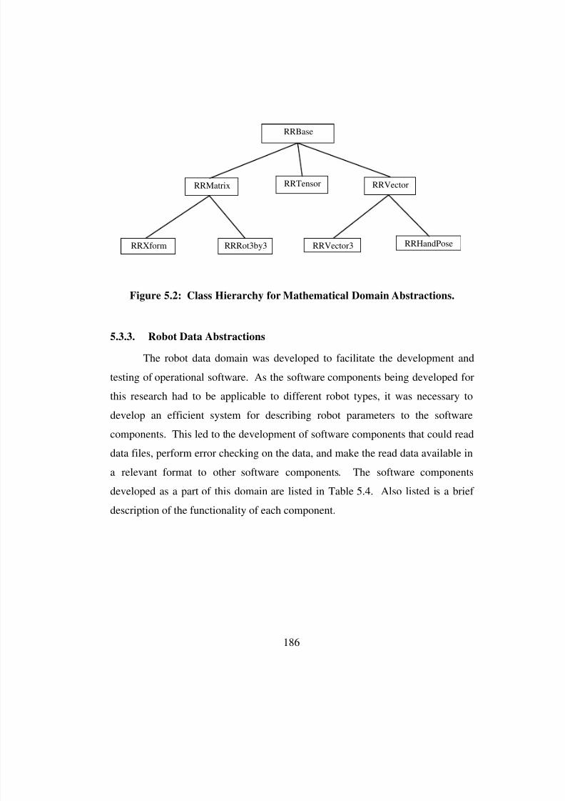
8/3/2019 Chetan Kapoor Dissertation
http://slidepdf.com/reader/full/chetan-kapoor-dissertation 210/612
186
5.3.3. Robot Data Abstractions
The robot data domain was developed to facilitate the development and
testing of operational software. As the software components being developed for
this research had to be applicable to different robot types, it was necessary to
develop an efficient system for describing robot parameters to the softwarecomponents. This led to the development of software components that could read
data files, perform error checking on the data, and make the read data available in
a relevant format to other software components. The software components
developed as a part of this domain are listed in Table 5.4. Also listed is a brief
description of the functionality of each component.
RRBase
RRMatrix
RRXform RRRot3by3
RRTensor RRVector
RRVector3 RRHandPose
Figure 5.2: Class Hierarchy for Mathematical Domain Abstractions.

8/3/2019 Chetan Kapoor Dissertation
http://slidepdf.com/reader/full/chetan-kapoor-dissertation 211/612
187
5.3.3.1. Robot Data
This software component is used to implement constructs that are
common to all components that read and parse data files. The analysis and design
details are given below:
Analysis
• The key attribute of this component is the name of the file that it reads data
from.
• Functionality should support opening and closing of files, counting of the total
number of tokens (valid data), and parsing through unwanted data (for
example, descriptive comments).
Design
Robot Data Component Description
Robot Data ⇒ Implements the functionality to open, close, and parsedata files
Matrix Data ⇒ Used to read data files that contain data in a matrixformat
⇒ Perform error checking on the data
Tensor Data ⇒ Used to read data files that contain data in a tensorformat
⇒ Perform error checking on the data
DH Data ⇒ Used to read data files that contain Denavit-Hartenbergparameters
⇒ Calculates the DOF of the robot and the type of joints(revolute or prismatic)
Table 5.4: Key Components of the Robot Data Domain.
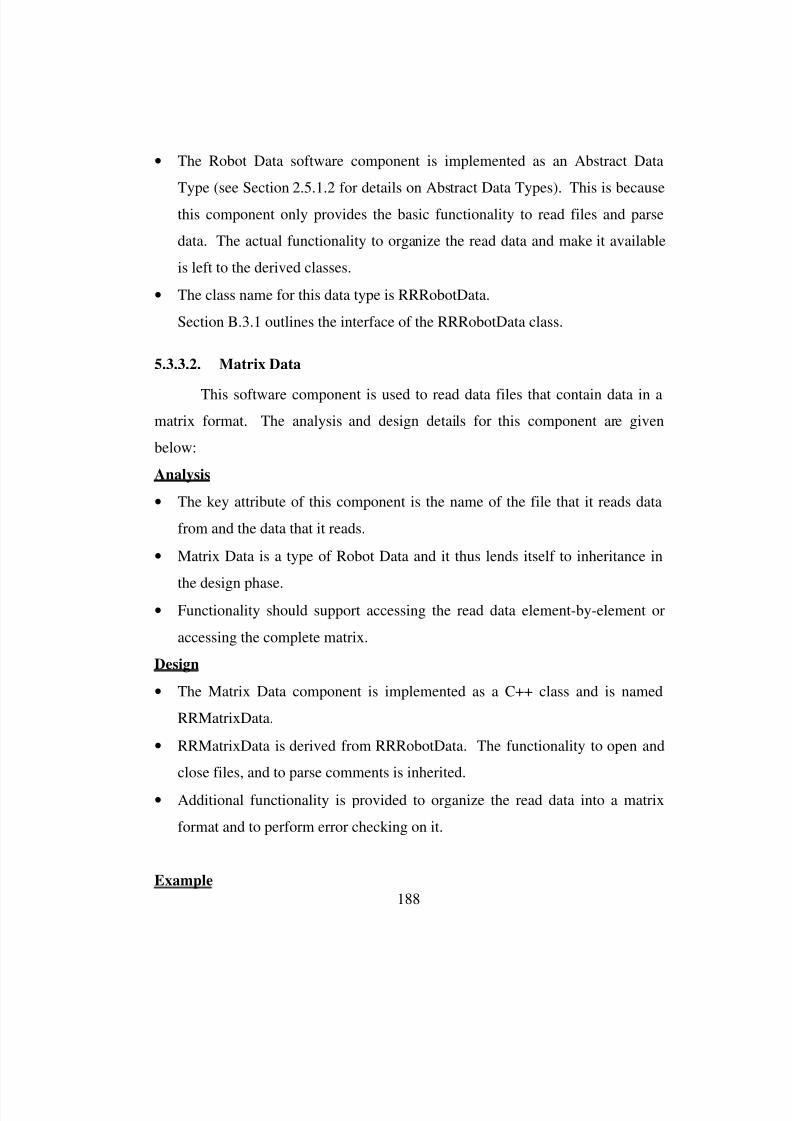
8/3/2019 Chetan Kapoor Dissertation
http://slidepdf.com/reader/full/chetan-kapoor-dissertation 212/612
188
• The Robot Data software component is implemented as an Abstract Data
Type (see Section 2.5.1.2 for details on Abstract Data Types). This is because
this component only provides the basic functionality to read files and parse
data. The actual functionality to organize the read data and make it available
is left to the derived classes.
• The class name for this data type is RRRobotData.
Section B.3.1 outlines the interface of the RRRobotData class.
5.3.3.2. Matrix Data
This software component is used to read data files that contain data in a
matrix format. The analysis and design details for this component are given
below:
Analysis
• The key attribute of this component is the name of the file that it reads data
from and the data that it reads.
• Matrix Data is a type of Robot Data and it thus lends itself to inheritance in
the design phase.• Functionality should support accessing the read data element-by-element or
accessing the complete matrix.
Design
• The Matrix Data component is implemented as a C++ class and is named
RRMatrixData.
• RRMatrixData is derived from RRRobotData. The functionality to open and
close files, and to parse comments is inherited.
• Additional functionality is provided to organize the read data into a matrix
format and to perform error checking on it.
Example
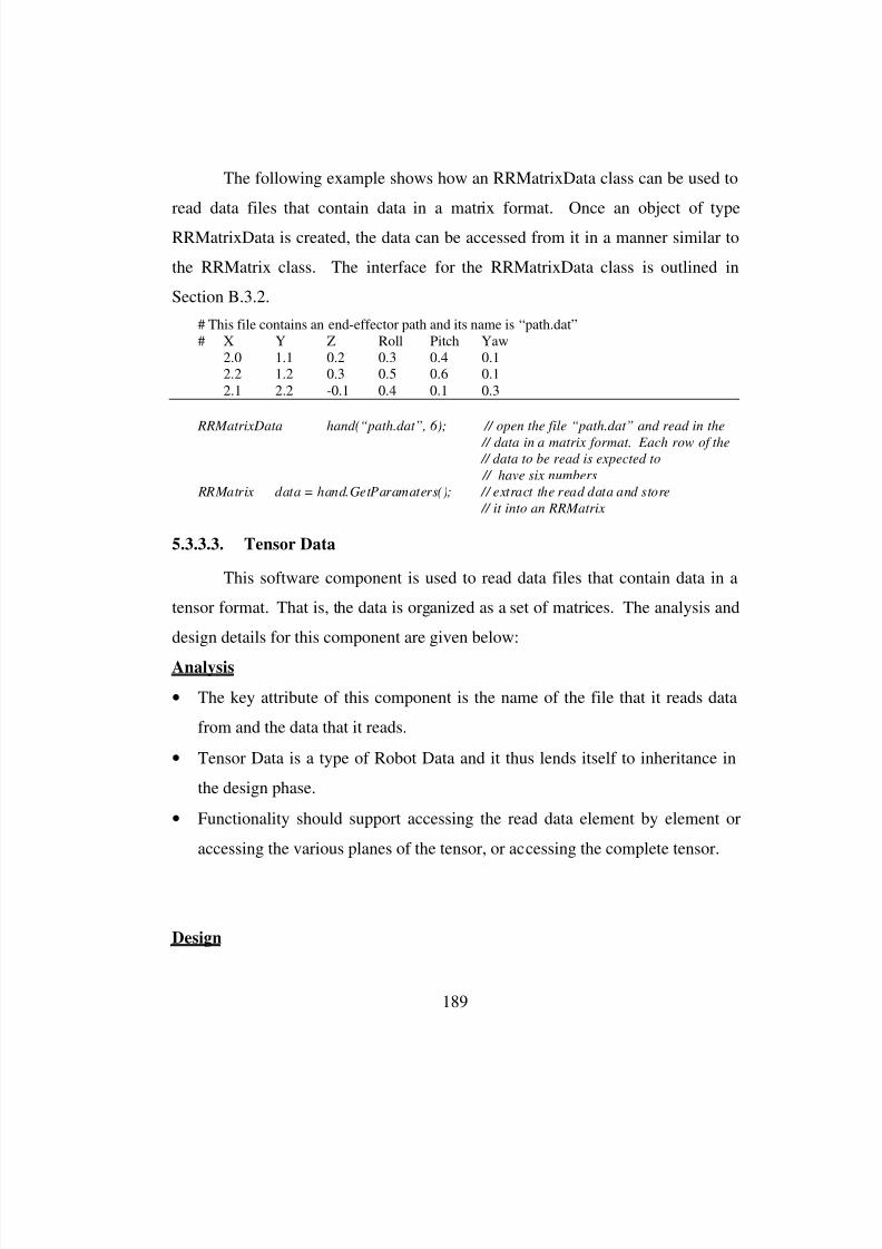
8/3/2019 Chetan Kapoor Dissertation
http://slidepdf.com/reader/full/chetan-kapoor-dissertation 213/612
189
The following example shows how an RRMatrixData class can be used to
read data files that contain data in a matrix format. Once an object of type
RRMatrixData is created, the data can be accessed from it in a manner similar to
the RRMatrix class. The interface for the RRMatrixData class is outlined in
Section B.3.2.
# This file contains an end-effector path and its name is “path.dat”# X Y Z Roll Pitch Yaw
2.0 1.1 0.2 0.3 0.4 0.12.2 1.2 0.3 0.5 0.6 0.12.1 2.2 -0.1 0.4 0.1 0.3
RRMatrixData hand(“path.dat”, 6); // open the file “path.dat” and read in the
// data in a matrix format. Each row of the // data to be read is expected to
// have six numbers
RRMatrix data = hand.GetParamaters(); // extract the read data and store
// it into an RRMatrix
5.3.3.3. Tensor Data
This software component is used to read data files that contain data in a
tensor format. That is, the data is organized as a set of matrices. The analysis and
design details for this component are given below:
Analysis
• The key attribute of this component is the name of the file that it reads data
from and the data that it reads.
• Tensor Data is a type of Robot Data and it thus lends itself to inheritance in
the design phase.
• Functionality should support accessing the read data element by element or
accessing the various planes of the tensor, or accessing the complete tensor.
Design
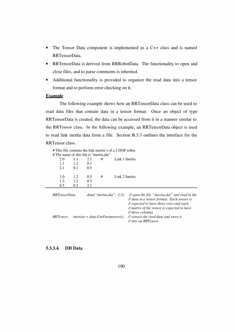
8/3/2019 Chetan Kapoor Dissertation
http://slidepdf.com/reader/full/chetan-kapoor-dissertation 214/612
190
• The Tensor Data component is implemented as a C++ class and is named
RRTensorData.
• RRTensorData is derived from RRRobotData. The functionality to open and
close files, and to parse comments is inherited.
• Additional functionality is provided to organize the read data into a tensor
format and to perform error checking on it.
Example
The following example shows how an RRTensorData class can be used to
read data files that contain data in a tensor format. Once an object of type
RRTensorData is created, the data can be accessed from it in a manner similar to
the RRTensor class. In the following example, an RRTensorData object is used
to read link inertia data from a file. Section B.3.3 outlines the interface for the
RRTensor class.
# This file contains the link inertia’s of a 2 DOF robot.# The name of this file is “inertia.dat”
2.0 1.1 2.1 # Link 1 Inertia1.1 1.2 0.12.1 0.1 0.5
1.0 1.2 0.5 # Link 2 Inertia1.2 1.2 0.30.5 0.3 2.1
RRTensorData data(“inertia.dat”, 3,3); // open the file “inertia.dat” and read in the
// data in a tensor format. Each tensor is
// expected to have three rows and each
// matrix of the tensor is expected to have
// three columns
RRTensor inertias = data.GetParameters(); // extract the read data and store it
// into an RRTensor
5.3.3.4. DH Data
8/3/2019 Chetan Kapoor Dissertation
http://slidepdf.com/reader/full/chetan-kapoor-dissertation 215/612
191
This software component is used to read data files that contain Denavit-
Hartenberg (DH) [Craig, 1986] parameter data for serial robots. The analysis and
design details for this component are given below:
Analysis
• The key attribute of this component is the name of the file that it reads data
from and the DH parameters that are read from the file.
• DH Data is a type of Robot Data and it thus lends itself to inheritance in the
design phase.
• Functionality should support accessing the values of the various DH
parameters, computing the DOF of the robot whose DH parameters are read,
and also decoding the type of the joint (revolute or prismatic) from the DH
parameter data.
Design
• The DH Data component is implemented as a C++ class and is named
RRDHData.
• RRDHData is derived from RRRobotData. The functionality to open and
close files, and to parse comments is inherited.
• Additional functionality is provided to organize the read data into a matrix
format, perform error checking, compute the DOF, and decode the type of
joint.
Example
The following example shows how an RRDHData class can be used to
read data files that contain DH parameter data. Once an object of type
RRDHData is created, the data can be accessed from it in a manner similar to anRRMatrix class. In the following example, an RRDHData object is used to read
in the DH parameters for a six DOF robot. Then the DOF of the robot and the
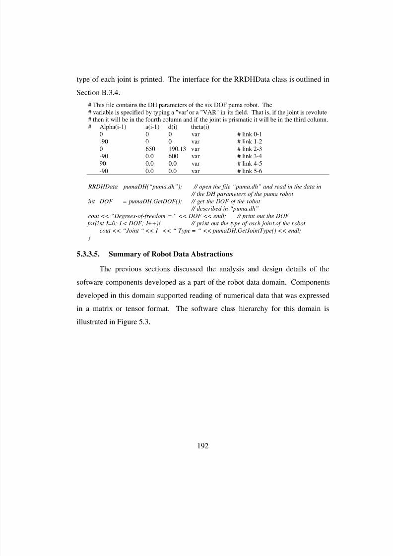
8/3/2019 Chetan Kapoor Dissertation
http://slidepdf.com/reader/full/chetan-kapoor-dissertation 216/612
192
type of each joint is printed. The interface for the RRDHData class is outlined in
Section B.3.4.
# This file contains the DH parameters of the six DOF puma robot. The# variable is specified by typing a "var’ or a "VAR" in its field. That is, if the joint is revolute# then it will be in the fourth column and if the joint is prismatic it will be in the third column.# Alpha(i-1) a(i-1) d(i) theta(i)
0 0 0 var # link 0-1-90 0 0 var # link 1-20 650 190.13 var # link 2-3-90 0.0 600 var # link 3-490 0.0 0.0 var # link 4-5-90 0.0 0.0 var # link 5-6
RRDHData pumaDH(“puma.dh”); // open the file “puma.dh” and read in the data in
// the DH parameters of the puma robot int DOF = pumaDH.GetDOF(); // get the DOF of the robot
// described in “puma.dh”
cout << “Degrees-of-freedom = “ << DOF << endl; // print out the DOF
for(int I=0; I < DOF; I++){ // print out the type of each joint of the robot
cout << “Joint “ << I << “ Type = “ << pumaDH.GetJointType() << endl;
}
5.3.3.5. Summary of Robot Data Abstractions
The previous sections discussed the analysis and design details of the
software components developed as a part of the robot data domain. Components
developed in this domain supported reading of numerical data that was expressed
in a matrix or tensor format. The software class hierarchy for this domain is
illustrated in Figure 5.3.
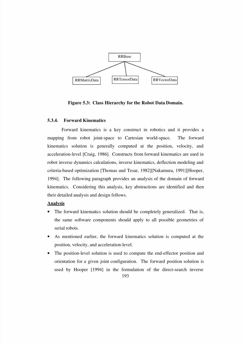
8/3/2019 Chetan Kapoor Dissertation
http://slidepdf.com/reader/full/chetan-kapoor-dissertation 217/612
193
5.3.4. Forward Kinematics
Forward kinematics is a key construct in robotics and it provides a
mapping from robot joint-space to Cartesian world-space. The forward
kinematics solution is generally computed at the position, velocity, and
acceleration-level [Craig, 1986]. Constructs from forward kinematics are used in
robot inverse dynamics calculations, inverse kinematics, deflection modeling and
criteria-based optimization [Thomas and Tesar, 1982][Nakamura, 1991][Hooper,
1994]. The following paragraph provides an analysis of the domain of forwardkinematics. Considering this analysis, key abstractions are identified and then
their detailed analysis and design follows.
Analysis
• The forward kinematics solution should be completely generalized. That is,
the same software components should apply to all possible geometries of
serial robots.
• As mentioned earlier, the forward kinematics solution is computed at the
position, velocity, and acceleration-level.
• The position-level solution is used to compute the end-effector position and
orientation for a given joint configuration. The forward position solution is
used by Hooper [1994] in the formulation of the direct-search inverse
RRBase
RRMatrixData RRTensorData RRVectorData
Figure 5.3: Class Hierarchy for the Robot Data Domain.
8/3/2019 Chetan Kapoor Dissertation
http://slidepdf.com/reader/full/chetan-kapoor-dissertation 218/612
194
kinematics scheme (see Chapter Three and Hooper [1994] for details).
Additionally, the Newton-Euler inverse dynamics formulation [Craig, 1986] is
based on the forward position solution.
• The forward kinematics solution at the velocity-level involves computing a
mapping between the joint velocities and the end-effector velocity. This
mapping is represented as the Jacobian matrix [Nakamura, 1991]. The
Jacobian matrix can be used for computing the inverse kinematics solution
using a technique called resolved rate motion control (see Chapter Three for
details).
• Further, kinematic influence coefficients as developed by Thomas and Tesar
[1982] are based on the forward kinematics solution at the velocity and
acceleration-level. These kinematic influence coefficients can be used in the
computation of the inverse dynamics solution [Thomas and Tesar, 1982], and
robot link deflections due to loads [Fresonke et al., 1988].
• It should be noted that even though the forward kinematics solution at the
position, velocity, and acceleration are separate sub-domains, the algorithms
that they are based on make them extensions of each other [Nakamura, 1991].
This is because, the forward acceleration solution is based on the forward
velocity solution, and the forward velocity solution is based on the forward
position solution.
Based on the analysis presented above, it was concluded that five key
components had to be developed to support functionality for computing the
forward kinematics solution. These components were identified as the forward
position solution, forward velocity solution, forward acceleration solution,
Jacobian level, and partial Jacobian. The Jacobian level component is a separate
component that only computes the Jacobian matrix. Even though, the
computation of the Jacobian matrix is also supported by the forward velocity

8/3/2019 Chetan Kapoor Dissertation
http://slidepdf.com/reader/full/chetan-kapoor-dissertation 219/612
195
solution, it was desired to have a simpler and smaller component for just
computing the Jacobian matrix. This is because the resolved rate motion control
technique relies exclusively on the Jacobian matrix. The partial Jacobian
component was created to facilitate the computation of the inverse kinematics
solution of a six DOF sub-structure of a redundant arm (see Chapter Three for
details on the algorithm). Table 5.5 lists the key components of the forward
kinematics domain.

8/3/2019 Chetan Kapoor Dissertation
http://slidepdf.com/reader/full/chetan-kapoor-dissertation 220/612
196
5.3.4.1. Position Level
This component encapsulates the forward kinematics solution at the
position-level for any serial robot. The (DH) parameters are used as inputs for
Forward Kinematics
Component
Description
Forward Position ⇒ Computes the hand position and orientationbased on an input joint configuration
⇒ Computes all local and global transformationmatrices
⇒ Allows adjustments for the tool-point and thelocation of the robot base frame with-respect-to the world frame
⇒ Takes the DH parameters as input
Jacobian Level ⇒ Computes the Jacobian matrix for the end-effector of a robot based on an input joint
configuration⇒ Jacobian level solution is an extension of the
position-level solution
Partial Jacobian ⇒ Computes the Jacobian matrix for a six DOFsub-structure of a redundant arm
⇒ Allows the ability to select the six joints thatconstitute the six DOF sub-structure
⇒ Partial Jacobian is an extension of theJacobian level solution
Forward Velocity ⇒ Computes the complete velocity-levelsolution based on input joint configuration
⇒ This includes the rotational and translationalfirst-order influence coefficients (see Thomas
and Tesar, [1982] for details)⇒ Forward velocity is an extension of theJacobian level solution
Forward Acceleration ⇒ Computes the complete acceleration-levelsolution based on input joint configuration
⇒ This includes the rotational and translationalsecond-order influence coefficients (seeThomas and Tesar [1982] for details)
⇒ Forward acceleration is an extension of theforward velocity-level solution
Table 5.5: Key Components of the Forward Kinematics Domain.
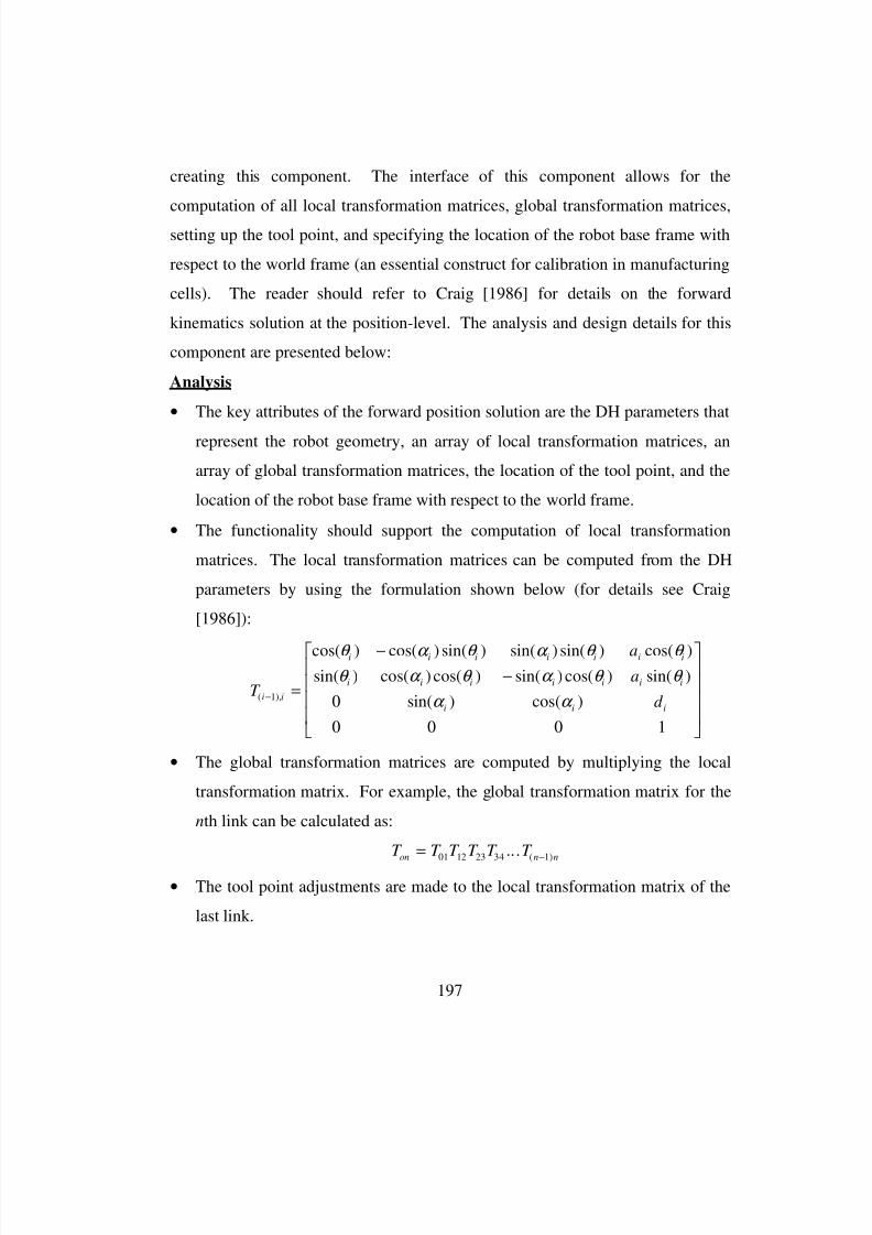
8/3/2019 Chetan Kapoor Dissertation
http://slidepdf.com/reader/full/chetan-kapoor-dissertation 221/612
197
creating this component. The interface of this component allows for the
computation of all local transformation matrices, global transformation matrices,
setting up the tool point, and specifying the location of the robot base frame with
respect to the world frame (an essential construct for calibration in manufacturing
cells). The reader should refer to Craig [1986] for details on the forward
kinematics solution at the position-level. The analysis and design details for this
component are presented below:
Analysis
• The key attributes of the forward position solution are the DH parameters that
represent the robot geometry, an array of local transformation matrices, an
array of global transformation matrices, the location of the tool point, and the
location of the robot base frame with respect to the world frame.
• The functionality should support the computation of local transformation
matrices. The local transformation matrices can be computed from the DH
parameters by using the formulation shown below (for details see Craig
[1986]):
T
a
a
d i i
i i i i i i i
i i i i i i i
i i i( ),
cos( ) cos( ) sin( ) sin( ) sin( ) cos( )sin( ) cos( ) cos( ) sin( ) cos( ) sin( )
sin( ) cos( )− =
−−
1 0
0 0 0 1
θ α θ α θ θ
θ α θ α θ θ
α α
• The global transformation matrices are computed by multiplying the local
transformation matrix. For example, the global transformation matrix for the
nth link can be calculated as:
T T T T T T on n n= −01 12 23 34 1... ( )
• The tool point adjustments are made to the local transformation matrix of the
last link.
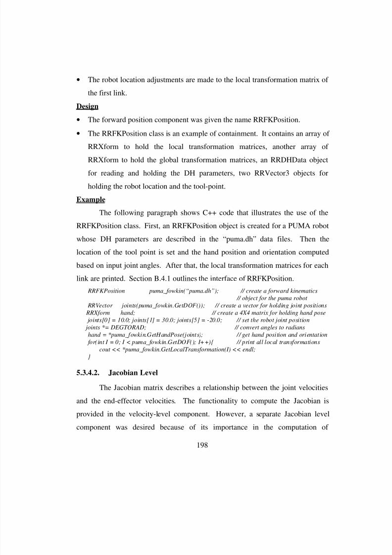
8/3/2019 Chetan Kapoor Dissertation
http://slidepdf.com/reader/full/chetan-kapoor-dissertation 222/612
198
• The robot location adjustments are made to the local transformation matrix of
the first link.
Design
• The forward position component was given the name RRFKPosition.
• The RRFKPosition class is an example of containment. It contains an array of
RRXform to hold the local transformation matrices, another array of
RRXform to hold the global transformation matrices, an RRDHData object
for reading and holding the DH parameters, two RRVector3 objects for
holding the robot location and the tool-point.
Example
The following paragraph shows C++ code that illustrates the use of the
RRFKPosition class. First, an RRFKPosition object is created for a PUMA robot
whose DH parameters are described in the “puma.dh” data files. Then the
location of the tool point is set and the hand position and orientation computed
based on input joint angles. After that, the local transformation matrices for each
link are printed. Section B.4.1 outlines the interface of RRFKPosition.
RRFKPosition puma_fowkin(“puma.dh”); // create a forward kinematics // object for the puma robot
RRVector joints(puma_fowkin.GetDOF()); // create a vector for holding joint positions
RRXform hand; // create a 4X4 matrix for holding hand pose
joints[0] = 10.0; joints[1] = 30.0; joints[5] = -20.0; // set the robot joint position
joints *= DEGTORAD; // convert angles to radians
hand = *puma_fowkin.GetHandPose(joints); // get hand position and orientation
for(int I = 0; I < puma_fowkin.GetDOF(); I++){ // print all local transformations
cout << *puma_fowkin.GetLocalTransformation(I) << endl;
}
5.3.4.2. Jacobian Level
The Jacobian matrix describes a relationship between the joint velocitiesand the end-effector velocities. The functionality to compute the Jacobian is
provided in the velocity-level component. However, a separate Jacobian level
component was desired because of its importance in the computation of
8/3/2019 Chetan Kapoor Dissertation
http://slidepdf.com/reader/full/chetan-kapoor-dissertation 223/612
199
generalized inverses and various performance criteria. This component “fine-
tunes” the computation of the Jacobian matrix and provides a simpler and cleaner
interface. The various analysis and design decisions faced in the development of
the Jacobian level component are given below:
Analysis
• The attributes of the Jacobian level component are the forward position
solution and the Jacobian matrix.
• This component should provide the functionality to compute the Jacobian
matrix based on an input joint angle configuration.
• As the attributes of a Jacobian level solution include the position solution, it
may lead us to believe that the position-level component (RRFKPosition)
should be contained inside the Jacobian level component. However, it was
decided to design the Jacobian level component as an extension of the
Position-level component. Using this approach, the Jacobian level component
just adds to the functionality of the position-level component.
• The elements of the Jacobian matrix can be computed from the global
transformation matrices using the formulation shown in Section 3.4.1.
Design
• The Jacobian level component was implemented as a C++ class and given the
name RRFKJacobian.
• As the Jacobian level solution is an extension of the position-level solution,
RRFKJacobian was derived from RRFKPosition.
• Functionality was defined to compute the individual columns of the Jacobian
matrix.• Additional functionality was added to compute the complete Jacobian and its
transpose.
Example

8/3/2019 Chetan Kapoor Dissertation
http://slidepdf.com/reader/full/chetan-kapoor-dissertation 224/612
200
The following example shows the use of the RRFKJacobian class. An
RRFKJacobian object is created for the robot whose DH parameters are described
in the “rr7.dh” data file. Using this object, the Jacobian matrix is computed for a
particular joint configuration. A pseudo-inverse of the Jacobian matrix is used to
compute the joint velocities based on some given hand velocities. Section B.4.2
outlines the interface of the RRFKJacobian class.
RRFKJacobian fkJacobian(“rr7.dh”); // create an RRFKJacobian object for the
// robot described by the DH parameters
// in the file” rr7.dh”
RRVector3 toolPoint; // create a vector to store the tool point of the robot
int DOF = fkJacbian.GetDOF(); // get the DOF of the robot in question
RRMatrix jacobian(6, DOF); // create a matrix that will hold the jacobian RRMatrix jacobianTrans(DOF, 6); // create a matrix for holding the jacobian transpose
RRVector jointPos(DOF); // create a vector for holding joint positions
RRVector jointVel(DOF); // create a vector for holding joint velocities
RRHandPose handVel(FIXED_XYZ); // create a vector for holding hand velocity
jointPos[0] = jointPos[1] = 10.0; // set joint 1 and 2 to 10 degrees
jointPos[4]= jointPos[6] = -4.0; // set joint 5 and 7 to -4.0 degrees
jointPos *= DEGTORAD; // convert joint angles from degrees to radians
handVel[0] = 1.0; // set hand X velocity = 1.0
handVel[1] = -3.0; // set hand Y velocity = -3.0
handVel[4] = 0.02; // set hand Roll angular velocity = 0.02
toolPoint.Z() = 10.0; // tool point is 10 units in the Z direction
fkJacobian.SetToolPoint(toolPoint); // convey the tool point information to fkJacobian jacobian = *fkJacobian.GetJacobian(jointPos); // compute jacobian based on joint position
jacobianTrans = *fkJacobian.GetJacobianTranspose(); // get jacobian transpose
if(DOF == 6){ // multiply hand velocity with the Jacobian inverse
jointVel = ~jacobian * handVel; // ~ is an operator overload for matrix inversion
}else if(DOF > 6){ // multiply hand velocity with the pseudo-inverse
jointVel =( jacobianTrans * (~(jacobian * jacobianTrans))) * handVel;
}
5.3.4.3. Partial Jacobian Level
This software component was developed to assist in the formulation of the
generalized hybrid inverse kinematics scheme described in Chapter Three. This
scheme uses a six DOF sub-structure to solve for the inverse position kinematics
8/3/2019 Chetan Kapoor Dissertation
http://slidepdf.com/reader/full/chetan-kapoor-dissertation 225/612
201
solution. The scheme used for solving the sub-structure inverse used resolved
rate motion control, which further relied on the Jacobian matrix. Thus, a software
component was needed that could compute the Jacobian matrix for a six DOF
sub-structure. The following paragraphs give the analysis and design details of
this software component.
Analysis
• The attributes of the partial Jacobian level component are the forward position
solution and the partial Jacobian matrix.
• This component should provide the functionality to compute the Jacobian
matrix for a six DOF sub-structure based on an input joint angle
configuration.
• Functionality should be provided to select any six joints for the partial
Jacobian. Support should also be provided to set the joint values of the
remaining joints (that is, lock the remaining joints). In essence, every time a
joint is locked to a different value, a new robot geometry is achieved. Thus,
for a ten DOF robot arm, four joints can be locked to arbitrary positions thus
achieving a six DOF robot.
• The Jacobian level component (RRFKJacobian) already provides the
functionality to compute individual columns of the Jacobian matrix. This
functionality is extended by the partial Jacobian component. This leads to an
inheritance relationship between the partial Jacobian component and the
Jacobian level component.
Design
• The partial Jacobian level was given the name RRFKPartialJacobian.
• As the partial Jacobian level solution is an extension of the Jacobian level
solution, RRFKPartialJacobian was derived from RRFKJacobian.
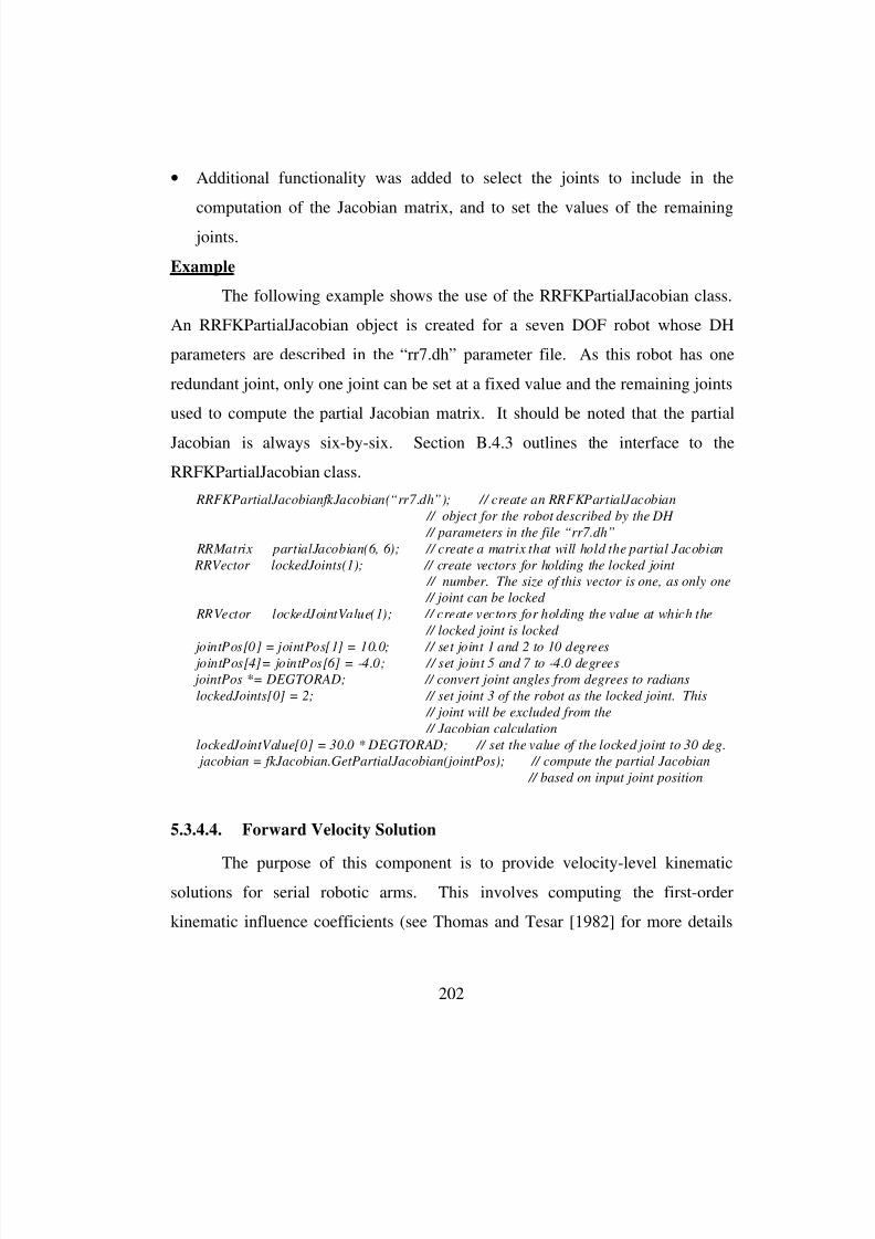
8/3/2019 Chetan Kapoor Dissertation
http://slidepdf.com/reader/full/chetan-kapoor-dissertation 226/612
202
• Additional functionality was added to select the joints to include in the
computation of the Jacobian matrix, and to set the values of the remaining
joints.
Example
The following example shows the use of the RRFKPartialJacobian class.
An RRFKPartialJacobian object is created for a seven DOF robot whose DH
parameters are described in the “rr7.dh” parameter file. As this robot has one
redundant joint, only one joint can be set at a fixed value and the remaining joints
used to compute the partial Jacobian matrix. It should be noted that the partial
Jacobian is always six-by-six. Section B.4.3 outlines the interface to the
RRFKPartialJacobian class.
RRFKPartialJacobian fkJacobian(“rr7.dh”); // create an RRFKPartialJacobian
// object for the robot described by the DH
// parameters in the file “rr7.dh”
RRMatrix partialJacobian(6, 6); // create a matrix that will hold the partial Jacobian
RRVector lockedJoints(1); // create vectors for holding the locked joint
// number. The size of this vector is one, as only one
// joint can be locked
RRVector lockedJointValue(1); // create vectors for holding the value at which the
// locked joint is locked
jointPos[0] = jointPos[1] = 10.0; // set joint 1 and 2 to 10 degrees jointPos[4]= jointPos[6] = -4.0; // set joint 5 and 7 to -4.0 degrees
jointPos *= DEGTORAD; // convert joint angles from degrees to radians
lockedJoints[0] = 2; // set joint 3 of the robot as the locked joint. This
// joint will be excluded from the
// Jacobian calculation
lockedJointValue[0] = 30.0 * DEGTORAD; // set the value of the locked joint to 30 deg.
jacobian = fkJacobian.GetPartialJacobian(jointPos); // compute the partial Jacobian
// based on input joint position
5.3.4.4. Forward Velocity Solution
The purpose of this component is to provide velocity-level kinematicsolutions for serial robotic arms. This involves computing the first-order
kinematic influence coefficients (see Thomas and Tesar [1982] for more details
8/3/2019 Chetan Kapoor Dissertation
http://slidepdf.com/reader/full/chetan-kapoor-dissertation 227/612
203
on kinematic influence coefficients). The analysis and design details for this
component are given below:
Analysis
• The attributes of this component are the forward position solution and the
rotational and translation first-order influence coefficients.
• The functionality provided by this component includes the computation of the
first-order translational and rotational influence coefficients.
• The computation of the kinematic influence coefficients uses the local and
global transformation matrices that were computed as a result of the forward
position solution. This would imply that this component should contain the
position-level component (RRFKPosition). However, it was decided to
develop the velocity-level component as an extension of the Jacobian level
component, which further is an extension of the position-level component.
This was done to gain access to the functionality of the position and Jacobian
level component and to expose the functionality of those components through
the interface of this component.
Design
• This component was implemented as a C++ class and given the name
RRFKVelocity.
• As this component is an extension of the Jacobian level solution,
RRFKVelocity is derived from RRFKJacobian. This class thus also supports
the functionality offered by RRFKJacobian and RRFKPosition.
• Functionality is provided for computing the first-order rotational influence
coefficients and first-order translational influence coefficients [Thomas andTesar, 1982]. The first-order influence coefficients can be computed for each
link of the robot and the translational influence coefficients can be computed
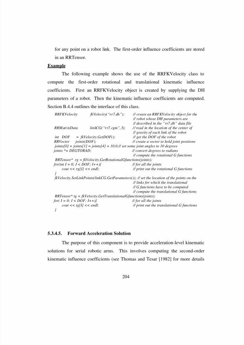
8/3/2019 Chetan Kapoor Dissertation
http://slidepdf.com/reader/full/chetan-kapoor-dissertation 228/612
204
for any point on a robot link. The first-order influence coefficients are stored
in an RRTensor.
Example
The following example shows the use of the RRFKVelocity class to
compute the first-order rotational and translational kinematic influence
coefficients. First an RRFKVelocity object is created by supplying the DH
parameters of a robot. Then the kinematic influence coefficients are computed.
Section B.4.4 outlines the interface of this class.
RRFKVelocity fkVelocity(“rr7.dh”); // create an RRFKVelocity object for the
// robot whose DH parameters are
// described in the “rr7.dh” data file
RRMatrixData linkCG(“rr7.cgm”,3); // read in the location of the center of
// gravity of each link of the robot
int DOF = fkVelocity.GetDOF(); // get the DOF of the robot
RRVector joints(DOF); // create a vector to hold joint positions
joints[0] = joints[1] = joints[4] = 10.0;// set some joint angles to 10 degrees
joints *= DEGTORAD; // convert degrees to radians
// compute the rotational G functions
RRTensor* rg = fkVelocity.GetRotationalGfunctions(joints);
for(int I = 0; I < DOF; I++){ // for all the joints
cout << rg[I] << endl; // print out the rotational G functions
}
fkVelocity.SetLinkPoints(linkCG.GetParameters()); // set the location of the points on the
// links for which the translational // G functions have to be computed
// compute the translational G functions
RRTensor* tg = fkVelocity.GetTranslationalGfunctions(joints);
for( I = 0; I < DOF; I++){ // for all the joints
cout << tg[I] << endl; // print out the translational G functions
}
5.3.4.5. Forward Acceleration Solution
The purpose of this component is to provide acceleration-level kinematic
solutions for serial robotic arms. This involves computing the second-order
kinematic influence coefficients (see Thomas and Tesar [1982] for more details
8/3/2019 Chetan Kapoor Dissertation
http://slidepdf.com/reader/full/chetan-kapoor-dissertation 229/612
205
on kinematic influence coefficients). The analysis and design details for this
component are given below:
Analysis
• The attributes of this component are the forward velocity solution and the
rotational and translation second-order influence coefficients.
• The functionality provided by this component includes the computation of the
second-order translational and rotational influence coefficients.
• The computation of the kinematic influence coefficients uses the first-order
influence coefficients that were computed as a result of the forward velocity
solution. This would imply that this component should contain the velocity-
level component (RRFKVelocity). However, the acceleration-level
component is developed as an extension to the velocity-level component.
This was done to gain access to the functionality of the velocity-level
component and to expose the functionality of the velocity-level component.
Design
• The acceleration-level component was implemented as a C++ class and given
the name RRFKAcceleration.
• As this component is an extension of the velocity-level component,
RRFKAcceleration is derived from RRFKVelocity. Thus, this class supports
the functionality offered by RRFKVelocity.
• Functionality is provided for computing the second-order rotational influence
coefficients and second-order translational influence coefficients [Thomas and
Tesar, 1982].
ExampleThe following example shows the use of the RRFKAcceleration class to
compute the second-order rotational and translational kinematic influence
coefficients. First an RRFKAcceleration object is created by supplying the DH
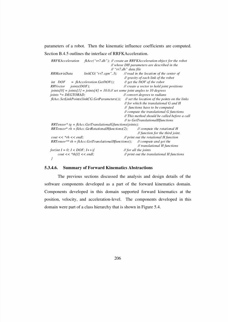
8/3/2019 Chetan Kapoor Dissertation
http://slidepdf.com/reader/full/chetan-kapoor-dissertation 230/612
206
parameters of a robot. Then the kinematic influence coefficients are computed.
Section B.4.5 outlines the interface of RRFKAcceleration.
RRFKAcceleration fkAcc(“rr7.dh”); // create an RRFKAcceleration object for the robot
// whose DH parameters are described in the
// “rr7.dh” data file
RRMatrixData linkCG(“rr7.cgm”,3); // read in the location of the center of
// gravity of each link of the robot
int DOF = fkAcceleration.GetDOF(); // get the DOF of the robot
RRVector joints(DOF); // create a vector to hold joint positions
joints[0] = joints[1] = joints[4] = 10.0;// set some joint angles to 10 degrees
joints *= DEGTORAD; // convert degrees to radians
fkAcc.SetLinkPoints(linkCG.GetParameters()); // set the location of the points on the links
// for which the translational G and H
// functions have to be computed
// compute the translational G functions. // This method should be called before a call
// to GetTranslationalHfunctions
RRTensor* tg = fkAcc.GetTranslationalGfunctions(joints);
RRTensor* rh = fkAcc.GetRotationalHfunctions(2); // compute the rotational H
// function for the third joint.
cout << *rh << endl; // print out the rotational H function
RRTensor** th = fkAcc.GetTranslationalHfunctions(); // compute and get the
// translational H functions
for(int I = 0; I < DOF; I++){ // for all the joints
cout << *th[I] << endl; // print out the translational H functions
}
5.3.4.6. Summary of Forward Kinematics Abstractions
The previous sections discussed the analysis and design details of the
software components developed as a part of the forward kinematics domain.
Components developed in this domain supported forward kinematics at the
position, velocity, and acceleration-level. The components developed in this
domain were part of a class hierarchy that is shown in Figure 5.4.
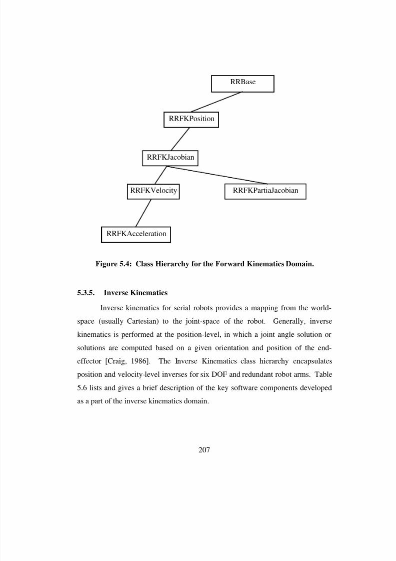
8/3/2019 Chetan Kapoor Dissertation
http://slidepdf.com/reader/full/chetan-kapoor-dissertation 231/612
207
RRBase
RRFKPosition
RRFKVelocity
RRFKAcceleration
RRFKJacobian
RRFKPartiaJacobian
Figure 5.4: Class Hierarchy for the Forward Kinematics Domain.
5.3.5. Inverse Kinematics
Inverse kinematics for serial robots provides a mapping from the world-
space (usually Cartesian) to the joint-space of the robot. Generally, inverse
kinematics is performed at the position-level, in which a joint angle solution or
solutions are computed based on a given orientation and position of the end-
effector [Craig, 1986]. The Inverse Kinematics class hierarchy encapsulates
position and velocity-level inverses for six DOF and redundant robot arms. Table
5.6 lists and gives a brief description of the key software components developed
as a part of the inverse kinematics domain.
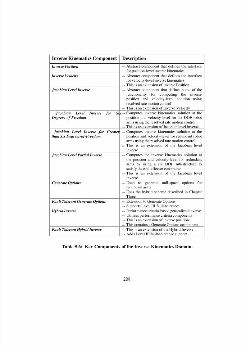
8/3/2019 Chetan Kapoor Dissertation
http://slidepdf.com/reader/full/chetan-kapoor-dissertation 232/612
208
Inverse Kinematics Component Description
Inverse Position ⇒ Abstract component that defines the interfacefor position-level inverse kinematics
Inverse Velocity ⇒ Abstract component that defines the interfacefor velocity-level inverse kinematics
⇒ This is an extension of Inverse Position
Jacobian Level Inverse ⇒ Abstract component that defines some of thefunctionality for computing the inverseposition and velocity-level solution usingresolved rate motion control
⇒ This is an extension of Inverse Velocity
Jacobian Level Inverse for Six
Degrees-of-Freedom
⇒ Computes inverse kinematics solution at theposition and velocity-level for six DOF robot
arms using the resolved rate motion control⇒ This is an extension of Jacobian level inverse
Jacobian Level Inverse for Greater
than Six Degrees-of-Freedom
⇒ Computes inverse kinematics solution at theposition and velocity-level for redundant robotarms using the resolved rate motion control
⇒ This is an extension of the Jacobian levelinverse
Jacobian Level Partial Inverse ⇒ Computes the inverse kinematics solution atthe position and velocity-level for redundantarms by using a six DOF sub-structure tosatisfy the end-effector constraints
⇒ This is an extension of the Jacobian levelinverse
Generate Options ⇒ Used to generate null-space options forredundant arms
⇒ Uses the hybrid scheme described in ChapterThree
Fault Tolerant Generate Options ⇒ Extension to Generate Options⇒ Supports Level III fault-tolerance
Hybrid Inverse ⇒ Performance criteria-based generalized inverse⇒ Utilizes performance criteria components⇒ This is an extension of inverse position⇒ This contains a Generate Options component
Fault Tolerant Hybrid Inverse ⇒ This is an extension of the Hybrid Inverse⇒ Adds Level III fault-tolerance support
Table 5.6: Key Components of the Inverse Kinematics Domain.
8/3/2019 Chetan Kapoor Dissertation
http://slidepdf.com/reader/full/chetan-kapoor-dissertation 233/612
209
5.3.5.1. Position Level
The inverse position solution for robots involves computing the jointpositions based on an input end-effector position and orientation. RRIKPosition
merely implements the interface without specifying any functionality (hence an
abstract data type). The functionality is defined in the derived classes. The
interface for this class provides functions that compute the inverse position
solution based on a given hand transformation matrix (RRXform) or a six element
vector that specifies the position and orientation of the hand (RRHandPose).
Additional functionality is provided for setting the tool point coordinates, and the
robot base frame location with respect to the world frame. Section B.5.1 outlines
the interface of the RRIKPosition class.
5.3.5.2. Velocity Level
The inverse kinematics solution at the velocity-level involves computing
the joint velocities based on input end-effector velocities. This component is
implemented as an abstract data type and is named RRIKVelocity. Additionally,
RRIKVelocity is derived from RRIKPosition and it extends its interface toinclude functions for computing the joint velocities based on input hand
velocities. As RRIKVelocity is also an abstract data type, the functionality is
provided by derived classes. Section B.5.2 outlines the interface to the
RRIKVelocity class.
5.3.5.3. Jacobian Level Inverse
The purpose of this component is to provide functionality for computing
the generalized inverse using the resolved rate motion control technique
[Whitney, 1969]. The analysis and design details of this component are given
below:
Analysis
8/3/2019 Chetan Kapoor Dissertation
http://slidepdf.com/reader/full/chetan-kapoor-dissertation 234/612
210
• The key input to this component is the hand position and orientation of the
end-effector. The desired output is the joint position that satisfies the input
hand positions. Additionally, as resolved rate motion control is based on a
velocity-level formulation, another input to this component is the hand
velocity. The desired output for this is the joint velocities.
• The resolved rate motion control technique is based on using the Jacobian
matrix to compute the joint velocities based on a given input hand velocity.
This is expressed as:
x J q. .
=where x
.
is a vector of hand velocities, J is the Jacobian matrix, and q.
is a
vector of joint velocities. By inverting the Jacobian matrix, the joint
velocities can be expressed in terms of the hand velocities. This is expressed
as:
q J x.
1.
= −
Further on, this can be expressed as a differential relationship between the
joint displacements and the end-effector displacements. This is expressed as:
dq J dx1= −
where, dq is the differential joint vector, J is the Jacobian matrix, and dx is
the differential hand vector. The relationship shown above can be iterated
over until the error between the desired hand position and the actual hand
position is within acceptable error bounds. Note that the computation of the
Jacobian inverse depends upon its size and the optimizations and robustness
desired. For example, for a six DOF robot, the Jacobian matrix is six-by-six
and a simple inverse based on Gaussian elimination may be sufficient.
However, if a redundant arm is in consideration, a pseudo-inverse may be
needed or a singularity robust inverse may be desired. The reader should refer
8/3/2019 Chetan Kapoor Dissertation
http://slidepdf.com/reader/full/chetan-kapoor-dissertation 235/612
211
to Nakamura [1991] for details on different formulations for inverting the
Jacobian matrix and computing the differential joint vector based on the input
differential hand vector.
Design
The analysis provided above outlined the steps in the computation of the
inverse kinematics solution. Based on these steps, the following design
specifications were generated:
• This component is named RRIKJacobian.
• The analysis showed the reliance of the inverse solution on the Jacobian
matrix. Hence, this component had to support functionality for computing the
Jacobian matrix. This functionality was supported using containment. That
is, an RRFKJacobian object was contained within this component. The
RRFKJacobian component was used to supply the Jacobian matrix. Further,
the user has the option to supply a custom RRFKJacobian object to
RRIKJacobian or use the default RRFKJacobian object that is contained
inside the RRIKJacobian. The advantage of this is that the user can supply
the RRIKJacobian with an object that is derived from RRFKJacobian. The
user derived RRFKJacobian object may implement a more efficient method of
computing the Jacobian matrix thereby improving the computational
efficiency of RRIKJacobian.
• As this inverse solution relies on iteration, functionality was designed to allow
setting an upper bound on the iterations. Further, functionality was supplied
to detect singularities.
• Functionality was also added in three other areas. These were, functionality
to compute the error, functionality to perform the iterations until the solution
converged, and functionality to compute the differential joint vector based on
an error hand vector.
8/3/2019 Chetan Kapoor Dissertation
http://slidepdf.com/reader/full/chetan-kapoor-dissertation 236/612
212
• As mentioned in the analysis, the technique used to compute the differential
joint vector can vary based on the DOF of the robot, and the type of the
desired solution (minimum-norm, singularity robust, joint limit avoidance,
etc.). Hence, the functionality for computing the differential joint vector was
not defined in this class. It was left to the derived classes to supply this
functionality.
Section B.5.3 outlines the interface of the RRIKJacobian class.
5.3.5.4. Jacobian Level Inverse For Six Degrees-of-Freedom
This component provides the functionality to compute the inverse
kinematics solution for six DOF robots using the resolved rate motion control
technique [Whitney, 1969]. The key analysis and design issues for this
component are:
Analysis
• This component is a specialization of the Jacobian level inverse component.
• The key functionality of this component is to compute the differential joint
vector based on an error hand vector. For a six DOF robot, this can be doneusing the following formulation:
dq J dx1= −
• The functionality for iteration and computing the error solution is defined in
the base (RRIKJacobian) class.
Design
• This component was given the name RRIKJForSix and it is derived from
RRIKJacobian.
8/3/2019 Chetan Kapoor Dissertation
http://slidepdf.com/reader/full/chetan-kapoor-dissertation 237/612
213
• The method for computing the differential joint vector is defined in this class.
The functionality for iteration and error calculation is inherited from
RRIKJacobian.
Example
The following example shows the use of the RRIKJForSix class to
compute the inverse position solution for a six DOF robot arm. First an instance
of the RRIKJForSix class is created by supplying the DH parameters of the robot
under consideration. Also supplied are the starting initial joint angles and the
maximum desired error. Additionally, an RRFKPosition object is created to
evaluate the starting hand position based on the initial joint configuration. This
starting hand position provides a base point for the inverse kinematics. After that,
the RRIKJForSix object is used to compute the inverse position solution for
tracking a straight line path in the positive ‘X’ direction. Section B.5.4 outlines
the interface of the RRIKJforSix class.
RRFKPosition fowkin(“puma.dh”); // create a forward position object for
// the robot whose DH parameters are
// described in “puma.dh”
RRVector3 toolPoint; // create a vector to hold the tool point
RRVector initialJoints(fowkin.GetDOF())); // create a vector for holding initial // joint configuration
RRVector jointSolution(fowkin.GetDOF())); // create a vector for holding the solution of
// the inverse kinematics
toolPoint[2] = 13.0; // set the tool point to be 13 units in the ‘Z’
// direction of the local link frame of the
// last joint.
initialJoints[0] = 30.0; // set initial value of joint 1 to 30 degrees
initialJoints[2] = -60.0; ; // set initial value of joint 3 to -60 degrees
initialJoints[4] = 45.0; ; // set initial value of joint 5 to 45 degrees
RRXform hand; // create a 4X4 matrix to hold the end-
// effector position and orientation
initialJoints *= DEGTORAD; // convert angles from degrees to radians
fowkin.SetToolPoint(toolPoint); // inform fowkin of the tool point locationhand = *fowkin.GetHandPose(initialJoints); // compute the starting hand location
RRIKJForSixinvkin(“puma.dh”, initialJoints, 0.01); // create an inverse
// kinematics object for the robot whose DH
// parameters are given in “puma.dh.” The
// initial joint configuration and the

8/3/2019 Chetan Kapoor Dissertation
http://slidepdf.com/reader/full/chetan-kapoor-dissertation 238/612
214
// maximum error limit is also supplied
invkin.SetToolPoint(toolPoint); // inform invkin of the tool point location
for(int I = 0; I < 30; I++){ // increment the ’X’ coordinate of the
hand.at(0,3) += 0.1; // current hand location by 0.1 30 times
if(invkin.GetJointPosition(hand, jointSolution) > 0){ // and compute the inverse position
cout << jointSolution * RADTODEG << endl; // solution and print it
}else{ // if no solution
cout << “singularity” << endl; // print “singularity”
}
}
5.3.5.5. Jacobian Level Inverse For Greater than Six Degrees-of-Freedom
This component provides the functionality to compute the inverse
kinematics solution for redundant robots using the resolved rate motion control
technique [Nakamura, 1991]. The key analysis and design issues for this
component are:
Analysis
• This component is a specialization of the Jacobian level inverse component.
• The key functionality of this component is to compute the differential joint
vector based on an error hand vector. For a redundant robot, the differential
joint vector is computed as shown:
dq = J (J J ) dxt t 1−
,
This is also known as solving a linear system of equations using the pseudo
inverse. This formulation provides the minimum norm solution [Nakamura,
1991].
Design
• This component was given the name RRIKJForGTSix and it is derived from
RRIKJacobian.
• The method for computing the differential joint vector is defined in this class.
The other functionality for iteration and error calculation is inherited from
RRIKJacobian
Example
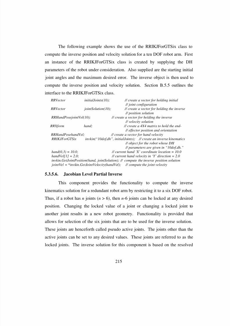
8/3/2019 Chetan Kapoor Dissertation
http://slidepdf.com/reader/full/chetan-kapoor-dissertation 239/612
215
The following example shows the use of the RRIKJForGTSix class to
compute the inverse position and velocity solution for a ten DOF robot arm. First
an instance of the RRIKJForGTSix class is created by supplying the DH
parameters of the robot under consideration. Also supplied are the starting initial
joint angles and the maximum desired error. The inverse object is then used to
compute the inverse position and velocity solution. Section B.5.5 outlines the
interface to the RRIKJForGTSix class.
RRVector initialJoints(10); // create a vector for holding initial
// joint configuration
RRVector jointSolution(10); // create a vector for holding the inverse
// position solution RRHandPosejointVel(10); // create a vector for holding the inverse
// velocity solution
RRXform hand; // create a 4X4 matrix to hold the end-
// effector position and orientation
RRHandPosehandVel; // create a vector for hand velocity
RRIKJForGTSix invkin(“10dof.dh”, initialJoints); // create an inverse kinematics
// object for the robot whose DH
// parameters are given in “10dof.dh.”
hand(0,3) = 10.0; // current hand ‘X’ coordinate location = 10.0
handVel[1] = 2.0; // current hand velocity in ‘Y’ direction = 2.0
invkin.GetJointPosition(hand, jointSolution); // compute the inverse position solution
jointVel = *invkin.GetJointVelocity(handVel); // compute the joint velocity
5.3.5.6. Jacobian Level Partial Inverse
This component provides the functionality to compute the inverse
kinematics solution for a redundant robot arm by restricting it to a six DOF robot.
Thus, if a robot has n joints (n > 6), then n-6 joints can be locked at any desired
position. Changing the locked value of a joint or changing a locked joint to
another joint results in a new robot geometry. Functionality is provided that
allows for selection of the six joints that are to be used for the inverse solution.
These joints are henceforth called pseudo active joints. The joints other than the
active joints can be set to any desired values. These joints are referred to as the
locked joints. The inverse solution for this component is based on the resolved

8/3/2019 Chetan Kapoor Dissertation
http://slidepdf.com/reader/full/chetan-kapoor-dissertation 240/612
216
rate motion control technique [Whitney, 1969]. The key analysis and design
issues for this component are:
Analysis
• This component is a specialization of the Jacobian level inverse component.
• The key functionality of this component is to compute the differential joint
vector based on an error hand vector. As this component always restricts a
redundant robot to six DOF, the differential joint vector can be computed
using the following formulation:
dq = J dx-1
• The functionality to compute a partial Jacobian based on the six active joints
is supplied by the RRFKPartialJacobian object. This object is contained
within this component.
• The functionality for iterating until error bounds are satisfied is redefined to
take into account the locking of joints.
• Functionality is added to support the locking of joints.
• The functionality for computing the error solution is defined in the
RRIKJacobian class.
Design
• This component was given the name RRIKJPartial and it is derived from
RRIKJacobian.
• The methods for computing the differential joint vector and iterating until the
error bounds are satisfied are redefined in this class. The functionality for
error calculation is inherited from RRIKJacobian.
• Additional functionality for specifying the joints to be locked, the values at
which to lock the joints, and getting the status of a joint (locked or active) is
also provided.
Example
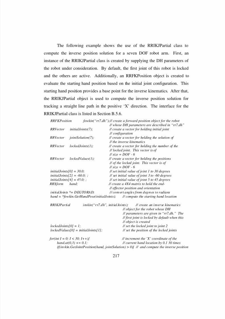
8/3/2019 Chetan Kapoor Dissertation
http://slidepdf.com/reader/full/chetan-kapoor-dissertation 241/612
217
The following example shows the use of the RRIKJPartial class to
compute the inverse position solution for a seven DOF robot arm. First, an
instance of the RRIKJPartial class is created by supplying the DH parameters of
the robot under consideration. By default, the first joint of this robot is locked
and the others are active. Additionally, an RRFKPosition object is created to
evaluate the starting hand position based on the initial joint configuration. This
starting hand position provides a base point for the inverse kinematics. After that,
the RRIKJPartial object is used to compute the inverse position solution for
tracking a straight line path in the positive ‘X’ direction. The interface for the
RRIKJPartial class is listed in Section B.5.6.
RRFKPosition fowkin(“rr7.dh”);// create a forward position object for the robot
// whose DH parameters are described in “rr7.dh”
RRVector initialJoints(7); // create a vector for holding initial joint
// configuration
RRVector jointSolution(7); // create a vector for holding the solution of
// the inverse kinematics
RRVector lockedJoints(1); // create a vector for holding the number of the
// locked joint. This vector is of
// size = DOF - 6
RRVector lockedValues(1); // create a vector for holding the positions
// of the locked joint. This vector is of
// size = DOF - 6 initialJoints[0] = 30.0; // set initial value of joint 1 to 30 degrees
initialJoints[2] = -60.0; ; // set initial value of joint 3 to -60 degrees
initialJoints[4] = 45.0; ; // set initial value of joint 5 to 45 degrees
RRXform hand; // create a 4X4 matrix to hold the end-
// effector position and orientation
initialJoints *= DEGTORAD; // convert angles from degrees to radians
hand = *fowkin.GetHandPose(initialJoints); // compute the starting hand location
RRIKJPartial invkin(“rr7.dh”, initialJoints); // create an inverse kinematics
// object for the robot whose DH
// parameters are given in “rr7.dh.” The
// first joint is locked by default when this
// object is created lockedJoints[0] = 1; // set the locked joint to joint 2
lockedValues[0] = initialJoints[1]; // set the position of the locked joints
for(int I = 0; I < 30; I++){ // increment the ’X’ coordinate of the
hand.at(0,3) += 0.1; // current hand location by 0.1 30 times
if(invkin.GetJointPosition(hand, jointSolution) > 0){ // and compute the inverse position

8/3/2019 Chetan Kapoor Dissertation
http://slidepdf.com/reader/full/chetan-kapoor-dissertation 242/612
218
cout << jointSolution * RADTODEG << endl; // solution and print it
}else{ // if no solution
cout << “singularity” << endl; // print “singularity”
}
}
5.3.5.7. Generate Options
The generate options component applies only to redundant arms and its
primary functionality is to support the generation of null-space joint options based
on a given end-effector location. In other words, once an end-effector location is
supplied to this component, it returns a set of joint angle solutions that satisfy the
end-effector constraints. This set of solutions is also known as the null-space orthe self-motions. The technique used for the generation of this self-motion is
described in detail in Chapter Three. This technique uses a hybrid formulation
that is based on a combination of a six DOF generalized inverse and the direct-
search technique (see Chapter Three for details). Using this scheme, a set of local
null-space joint options can be generated. Performance criteria can then be used
to rank this set of joint-space options. The best option can then be used as the
inverse kinematics solution. This component is slated for future development,
though its key functionality and its attributes have been finalized. These are:
• This component is created by supplying the DH parameters of the redundant
arm for which joint-space options have to be generated. Additionally, a
starting joint configuration of the arm and an error bound are also supplied.
• The key input into this system is an end-effector position and orientation. The
output is a set of joint-space options that satisfy the input position and
orientation.
• The number of options that are generated can be controlled. As this
component implements the hybrid scheme (see Chapter Three for details), it
supports simple, factorial, and exhaustive approaches to joint-space options
generation.

8/3/2019 Chetan Kapoor Dissertation
http://slidepdf.com/reader/full/chetan-kapoor-dissertation 243/612
219
• The hybrid scheme uses a generalized inverse for computing the inverse
position solution for a six DOF substructure of the redundant arm. The
functionality to compute this sub-structure inverse is supported by
RRIKJPartial class. Thus, the RRIKJPartial class is contained within the
generate options component.
• Functionality is provided to perform direct-search on the joints to generate a
set of joint-space options.
• Though this component does not output an inverse position solution, it is still
a part of the inverse kinematics domain. This is because of the algorithmic
compatibility of this component with the inverse kinematics domain.
• This component is given the name RRGenerateOptions and is derived from
the RRBase class.
5.3.5.8. Fault Tolerant Generate Options
This component is an extension to the generate options component
described in the previous section. The purpose of this component is to add level
III fault-tolerance to the generate options component. Level III fault-tolerancerelies on redundancy to counteract joint failure [Sreevijayan and Tesar, 1994].
Thus, this component adds the functionality to allow for joint-space options
generation in the event of joint failure. The key functionality and attributes of
this component have been finalized and are discussed below:
• This component is an extension of the generate options component and is thus
derived from it. All the functionality of the generate options component is
inherited by this component.
• The name of this component is RRFTGenerateOptions.
• An RRFTGenerateOptions object can be created by supplying the DH
parameters of the redundant arm for which joint-space options have to be
generated.
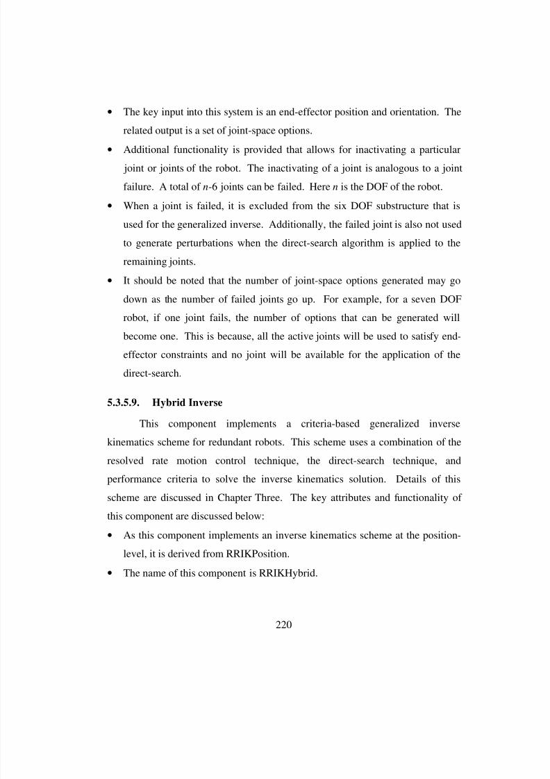
8/3/2019 Chetan Kapoor Dissertation
http://slidepdf.com/reader/full/chetan-kapoor-dissertation 244/612
220
• The key input into this system is an end-effector position and orientation. The
related output is a set of joint-space options.
• Additional functionality is provided that allows for inactivating a particular
joint or joints of the robot. The inactivating of a joint is analogous to a joint
failure. A total of n-6 joints can be failed. Here n is the DOF of the robot.
• When a joint is failed, it is excluded from the six DOF substructure that is
used for the generalized inverse. Additionally, the failed joint is also not used
to generate perturbations when the direct-search algorithm is applied to the
remaining joints.
• It should be noted that the number of joint-space options generated may go
down as the number of failed joints go up. For example, for a seven DOF
robot, if one joint fails, the number of options that can be generated will
become one. This is because, all the active joints will be used to satisfy end-
effector constraints and no joint will be available for the application of the
direct-search.
5.3.5.9. Hybrid Inverse
This component implements a criteria-based generalized inverse
kinematics scheme for redundant robots. This scheme uses a combination of the
resolved rate motion control technique, the direct-search technique, and
performance criteria to solve the inverse kinematics solution. Details of this
scheme are discussed in Chapter Three. The key attributes and functionality of
this component are discussed below:
• As this component implements an inverse kinematics scheme at the position-
level, it is derived from RRIKPosition.
• The name of this component is RRIKHybrid.
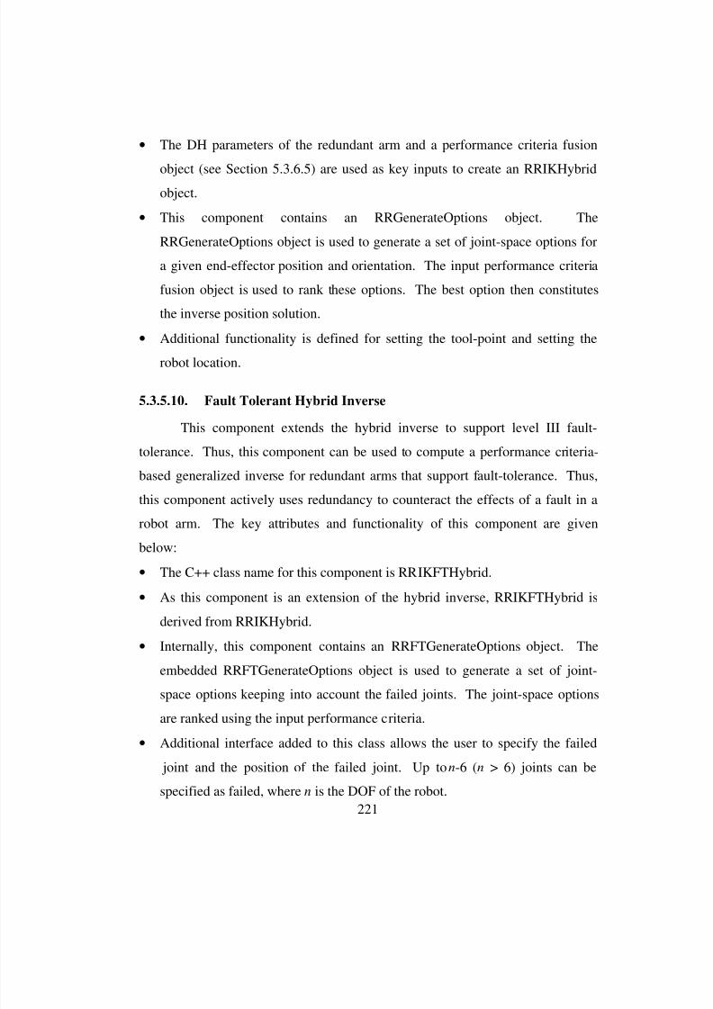
8/3/2019 Chetan Kapoor Dissertation
http://slidepdf.com/reader/full/chetan-kapoor-dissertation 245/612
221
• The DH parameters of the redundant arm and a performance criteria fusion
object (see Section 5.3.6.5) are used as key inputs to create an RRIKHybrid
object.
• This component contains an RRGenerateOptions object. The
RRGenerateOptions object is used to generate a set of joint-space options for
a given end-effector position and orientation. The input performance criteria
fusion object is used to rank these options. The best option then constitutes
the inverse position solution.
• Additional functionality is defined for setting the tool-point and setting the
robot location.
5.3.5.10. Fault Tolerant Hybrid Inverse
This component extends the hybrid inverse to support level III fault-
tolerance. Thus, this component can be used to compute a performance criteria-
based generalized inverse for redundant arms that support fault-tolerance. Thus,
this component actively uses redundancy to counteract the effects of a fault in a
robot arm. The key attributes and functionality of this component are givenbelow:
• The C++ class name for this component is RRIKFTHybrid.
• As this component is an extension of the hybrid inverse, RRIKFTHybrid is
derived from RRIKHybrid.
• Internally, this component contains an RRFTGenerateOptions object. The
embedded RRFTGenerateOptions object is used to generate a set of joint-
space options keeping into account the failed joints. The joint-space options
are ranked using the input performance criteria.
• Additional interface added to this class allows the user to specify the failed
joint and the position of the failed joint. Up to n-6 (n > 6) joints can be
specified as failed, where n is the DOF of the robot.
8/3/2019 Chetan Kapoor Dissertation
http://slidepdf.com/reader/full/chetan-kapoor-dissertation 246/612
222
5.3.5.11. Closed-Form Inverse
The previous sections discussed the analysis and design of componentsthat support generalized kinematics. Closed-form kinematics offers the
advantages of execution speed and robustness over generalized kinematics. Thus,
an abstract data type was developed that supported closed-form inverse
kinematics. For this purpose, a new data type called RRIKClosedForm was
derived from RRIKPosition. This class acts as a base class for all closed-form
inverse position solutions. As this class encapsulates closed-form solutions, the
functionality for checking the maximum number of iterations, setting the tool-
point, and the maximum error is redefined. Functionality for checking the
maximum number of iterations and maximum error is not needed here because it
is a closed-form solution. A closed-form inverse always produces a zero error
solution (barring numerical error) unless the robot is in a singular configuration.
5.3.5.12. Puma Geometry Inverse
RRIKPumaGeometry is derived from RRIKClosedForm and it
implements a closed-form inverse position solution for wrist point robots thathave a similar geometry to the PUMA 560 industrial robot.
5.3.5.13. Summary of The Inverse Kinematics Domain
The previous sections discussed the analysis and design details of the
software components developed as a part of the inverse kinematics domain.
Components developed in this domain supported generalized and closed-form
inverse kinematics at the position and velocity-level. The components developed
in this domain were part of a class hierarchy that is shown in Figure 5.5.

8/3/2019 Chetan Kapoor Dissertation
http://slidepdf.com/reader/full/chetan-kapoor-dissertation 247/612
223
RRIKPosition
RRIKVelocity
RRIKJacobian
RRIKJForGTSix RRIKJPartialRRIKJForSix
RRIKClosedForm
RRIKPumaGeometry
RRIKHybrid
RRIKFTHybrid
RRBase
RRGenerateOptions
RRFTGenerateOptions
Figure 5.5: Class Hierarchy for the Inverse Kinematics Domain.
5.3.6. Performance CriteriaThe inverse kinematics solution of redundant robot arms has infinite
solutions. This property of redundant arms can be used to appropriately select a
solution that maximizes a certain performance criterion or a set of performance
criteria. Initially, five general categories of these performance criteria have been
identified. These are constraint, geometric, inertial, compliance, and kinetic
energy [Hooper, 1994]. This domain includes components for performance
criteria and criteria fusion. Table 5.7 lists and gives a brief description of the key
software components developed as a part of the performance criteria domain.
These components are described in detail in the following sections.
Performance Criteria Description

8/3/2019 Chetan Kapoor Dissertation
http://slidepdf.com/reader/full/chetan-kapoor-dissertation 248/612
224
Components
Performance Criteria ⇒ Abstract component that defines theinterface and some functionality for variousperformance criteria.
⇒ Includes functionality for sorting
Maximize Joint Range Availability ⇒ Component that ranks various joint-spaceoptions based on the joint range availabilityor distance from joint limits
⇒ This is an extension of performance criteria
Minimize Joint Velocity ⇒ Component that ranks various joint-spaceoptions based on the joint velocities
⇒ This is an extension of performance criteria
Maximize Measure of Transmissibility ⇒ Component that ranks various joint-spaceoptions based on distance from singularity
⇒ This is an extension of performance criteria
Criteria Fusion ⇒ Component for fusing various criteria andcoming up with an overall ranking of joint-space options
⇒ Includes functionality for sorting⇒ Uses the weighted sum technique described
in Chapter Three
Table 5.7: Key Components of the Performance Criteria Domain.
5.3.6.1. Performance Criteria
The purpose of this component is to provide functionality that is common
to the development of specific performance criteria. Analysis and design
considerations for this component are given below:
Analysis
• The key input for this component is a set of joint angle solutions that satisfy a
particular end-effector constraint. The output of this component is a ranking
of the input solutions based on some relevant criteria.
• The functionality to compute a criteria value is specific to a particular criteria
and is left to the derived classes.
8/3/2019 Chetan Kapoor Dissertation
http://slidepdf.com/reader/full/chetan-kapoor-dissertation 249/612
225
• A sorting algorithm has to be used in this component for ranking various
options.
• Each criteria has a weight associated with it. Additionally, a criteria can be
maximized or minimized.
Design
• This component was given the name RRPerformanceCriteria.
• RRPerformanceCriteria is implemented as an abstract data type because it
only provides an interface for computing criteria value. The functionality is
left to the derived classes.
• RRPerformanceCriteria is derived from RRBase.
• The functionality to sort solutions is provided in this class and is used by all
derived classes. The quick-sort algorithm is used for ranking input options
[Horowitz and Sahni, 1993].
• Functionality is provided for accessing and setting the weight of a criterion,
and setting whether a criterion needs to be maximized or minimized.
Section B.6.1 outlines the interface of the RRPerformanceCriteria class.
5.3.6.2. Maximize Joint Range Availability
This component implements a constraint criteria that is based on
maximizing the Joint Range Availability (JRA). The analysis and design issues
for this component are given below:
Analysis
• Maximize Joint Range Availability is a type of performance criteria. This
implies an IS-A relationship.
• The JRA is represented and formulated as follows:

8/3/2019 Chetan Kapoor Dissertation
http://slidepdf.com/reader/full/chetan-kapoor-dissertation 250/612
226
JRA =
i i
ii=
nθ θ
θ
−
∑
~
max
2
21 ,
where i is the joint displacement, iθ
~
is the mid-range displacement and i max
is the displacement at the joint limit. This criterion seeks to select a joint
solution that keeps the joint displacements as near as possible to the midpoints
of their travel. This formulation is used to compute the criteria value.
Design
• This component is implemented as a C++ class and is named
RRPCAvoidLimits.
• As RRPCAvoidLimits is a type of performance criteria, it is derived from
RRPerformanceCriteria.
• The functionality for ranking various joint-space options, setting and
accessing the weight of a criteria, etc. is inherited from
RRPerformanceCriteria.
• The RRPerformanceCriteria class virtual method for computing criteria value
is defined in this class. It computes the criteria value based on the JRA.
Example
The following example shows a use of the RRPCAvoidLimits class to
rank various joint-space options based on their distance from joint limits. First an
RRPCAvoidLimits object is created by supplying the joint limits data for the
robot in question. Based on this joint limit data, the RRPCAvoidLimits object
can be queried for joint range and joint median. Further on, this object is used to
rank a set of joint-space options. The joint-space option that is furthest from the
joint limits (or closest to the median) is ranked at the top. Section B.6.2 outlines
the interface of this class.
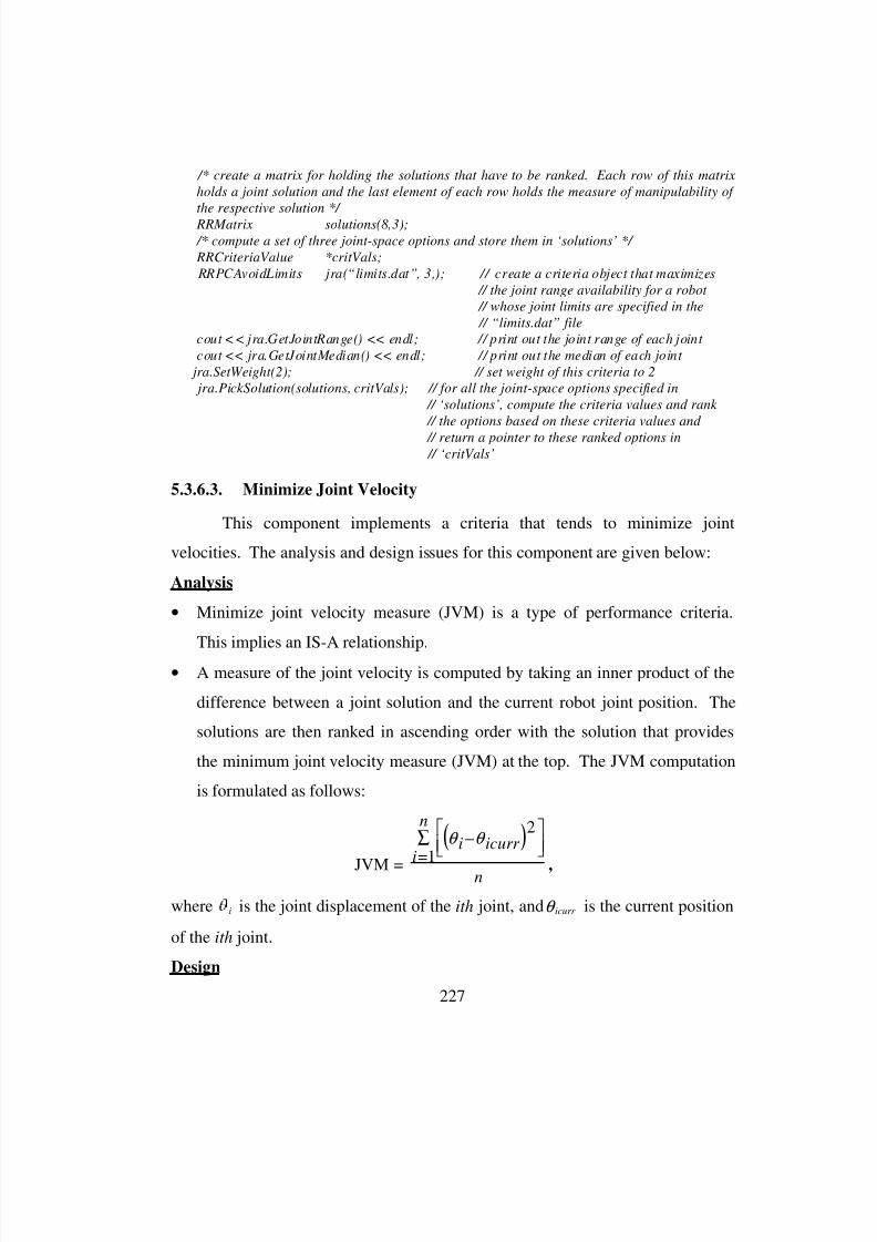
8/3/2019 Chetan Kapoor Dissertation
http://slidepdf.com/reader/full/chetan-kapoor-dissertation 251/612
227
/* create a matrix for holding the solutions that have to be ranked. Each row of this matrix
holds a joint solution and the last element of each row holds the measure of manipulability of
the respective solution */
RRMatrix solutions(8,3);
/* compute a set of three joint-space options and store them in ‘solutions’ */
RRCriteriaValue *critVals;
RRPCAvoidLimits jra(“limits.dat”, 3,); // create a criteria object that maximizes
// the joint range availability for a robot
// whose joint limits are specified in the
// “limits.dat” file
cout << jra.GetJointRange() << endl; // print out the joint range of each joint
cout << jra.GetJointMedian() << endl; // print out the median of each joint
jra.SetWeight(2); // set weight of this criteria to 2
jra.PickSolution(solutions, critVals); // for all the joint-space options specified in
// ‘solutions’, compute the criteria values and rank
// the options based on these criteria values and
// return a pointer to these ranked options in // ‘critVals’
5.3.6.3. Minimize Joint Velocity
This component implements a criteria that tends to minimize joint
velocities. The analysis and design issues for this component are given below:
Analysis
• Minimize joint velocity measure (JVM) is a type of performance criteria.
This implies an IS-A relationship.
• A measure of the joint velocity is computed by taking an inner product of the
difference between a joint solution and the current robot joint position. The
solutions are then ranked in ascending order with the solution that provides
the minimum joint velocity measure (JVM) at the top. The JVM computation
is formulated as follows:
( )
JVM =
i icurr i=
n
n
θ θ −
∑ 2
1
,
where i is the joint displacement of the ith joint, and icurr θ is the current position
of the ith joint.
Design
8/3/2019 Chetan Kapoor Dissertation
http://slidepdf.com/reader/full/chetan-kapoor-dissertation 252/612
228
• This component is implemented as a C++ class and is named
RRPCMinimizeVelocity.
• As RRPCMinimizeVelocity is a type of performance criteria, it is derived
from RRPerformanceCriteria.
• The functionality for ranking various joint-space options, setting and
accessing the weight of a criteria, etc. is inherited form
RRPerformanceCriteria.
• Additional functionality is provided for setting the current joint position of the
robot. This current position is used in computing the JVM for each joint-
space option.
• The RRPerformanceCriteria class virtual method for computing the criteria
value is defined in this class. It computes the criteria value based on the JVM.
Example
The following example shows a use of the RRPCMinimizeVelocity class
to rank various joint-space options based on their respective joint velocities. First
an RRPCMinimizeVelocity object is created by supplying the current joint
position of the robot. After that, joint-space options are supplied and the velocity
measure for each option is computed by subtracting each option from the current
joint position and taking the norm of the result. The joint-space option that
results in minimum joint velocity is ranked at the top.
/* create a matrix for holding the solutions that have to be ranked. Each row of this matrix
holds a joint solution and the last element of each row holds the measure of manipulability of
the respective solution */
RRMatrix solutions(8,3);
/* compute a set of three joint-space options and store them in ‘solutions’ */
RRVector currentPos; // current robot joint position
RRCriteriaValue *critVals; RRPCMinimizeVelocity jvm(currentPos, 3); // create a criteria object that
// minimizes the joint velocities
jvm.PickSolution(solutions, critVals); // for all the joint-space options specified in
// ‘solutions’, compute the criteria values and rank
// the options based on these criteria values and
// return a pointer to these ranked options in

8/3/2019 Chetan Kapoor Dissertation
http://slidepdf.com/reader/full/chetan-kapoor-dissertation 253/612
229
// ‘critVals’
5.3.6.4. Maximize Measure of Transmissibility
This component implements a criteria that seeks to select joint solutions
that have the maximum measure of transmissibility (MOT). The analysis and
design for this component are given below:
Analysis
• Maximize measure of transmissibility is a type of performance criteria. This
implies an IS-A relationship.
• MOT can be calculated as:
( )MOT
det T
=JJ
n 2
where J is the Jacobian matrix for a given joint position.
• The input joint solutions are sorted in descending order of MOT for each
solution.
Design
• This component is implemented as a class and is named
RRPCMaximizeMOT.
• As RRPCMaximizeMOT is a type of performance criteria, it is derived from
RRPerformanceCriteria.
• The functionality for ranking various joint-space options, setting and
accessing the weight of a criteria, etc. is inherited from
RRPerformanceCriteria.
• The RRPerformanceCriteria class virtual method for computing the criteria
value is defined in this class. It computes the criteria value based on the
MOT.
Example
8/3/2019 Chetan Kapoor Dissertation
http://slidepdf.com/reader/full/chetan-kapoor-dissertation 254/612
230
The following example shows a use of the RRPCMaximizeMOT class to
rank various joint-space options based on their respective measure of
transmissibility. First an RRPCMaximizeMOT object is created. After that,
joint-space options and their measure of transmissibility are supplied to the
RRPCMaximizeMOT object. The joint-space option with the maximum measure
of transmissibility is ranked at the top. Section B.6.4 outlines the interface of the
RRPCMaximizeMOT class.
/* create a matrix for holding the solutions that have to be ranked. Each row of this matrix
holds a joint solution and the last element of each row holds the measure of transmissibility of
the respective solution */
RRMatrix solutions(8,3); /* compute a set of three joint-space options and store them in ‘solutions’ */
RRCriteriaValue *critVals;
RRPCMaximizeMOT mot(3); // create a criteria object that
//maximizes the measure of transmissibility
mot.PickSolution(solutions, critVals); // for all the joint-space options specified in
// ‘solutions’, compute the criteria values and rank
// the options based on these criteria values and
// return a pointer to these ranked options in
// ‘critVals’
5.3.6.5. Performance Criteria Fusion
The previous sections showed the software components developed forsingle criterion-based decision making. However, in a “real-world” application,
multiple criteria are actively used in decision making. For example, in a “real”
application, it is equally important to avoid joint limits and to avoid singularities.
Criteria fusion is one means of incorporating multiple criteria. This software
component implements a scheme for criteria fusion that is based on a weighted
sum (see Chapter Three for more details). The analysis and design issues faced in
the development of this component are discussed below:
Analysis
• The two key inputs for this software component are a set of performance
criteria and a set of joint-space options. The key output of this system is an
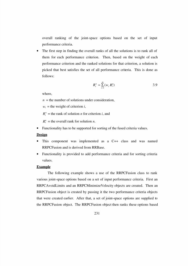
8/3/2019 Chetan Kapoor Dissertation
http://slidepdf.com/reader/full/chetan-kapoor-dissertation 255/612
231
overall ranking of the joint-space options based on the set of input
performance criteria.
• The first step in finding the overall ranks of all the solutions is to rank all of
them for each performance criterion. Then, based on the weight of each
performance criterion and the ranked solutions for that criterion, a solution is
picked that best satisfies the set of all performance criteria. This is done as
follows:
R w Rt
n
i in
i
m
= ∑=
( )1
3.9
where,
n = the number of solutions under consideration,
iw = the weight of criterion i,
Ri
n = the rank of solution n for criterion i, and
t n R = the overall rank for solution n.
• Functionality has to be supported for sorting of the fused criteria values.
Design
• This component was implemented as a C++ class and was named
RRPCFusion and is derived from RRBase.
• Functionality is provided to add performance criteria and for sorting criteria
values.
Example
The following example shows a use of the RRPCFusion class to rank
various joint-space options based on a set of input performance criteria. First an
RRPCAvoidLimits and an RRPCMinimizeVelocity objects are created. Then anRRPCFusion object is created by passing it the two performance criteria objects
that were created earlier. After that, a set of joint-space options are supplied to
the RRPCFusion object. The RRPCFusion object then ranks these options based
8/3/2019 Chetan Kapoor Dissertation
http://slidepdf.com/reader/full/chetan-kapoor-dissertation 256/612
232
on a fusion of the input performance criteria set. Section B.6.5 outlines the
interface of the RRPCFusion class.
/* create a matrix for holding the solutions that have to be ranked. Each row of this matrix
holds a joint solution and the last element of each row holds the measure of transmissibility of
the respective solution */
RRMatrix solutions(8,3);
/* compute a set of three joint-space options and store them in ‘solutions’ */
RRVector currentPos; // current robot joint position
RRCriteriaValue *critVals;
RRPCAvoidLimits jra(“limits.dat”, 3,); // create a criteria object that maximizes
// the joint range availability for a robot
// whose joint limits are specified in the
// “limits.dat” file
RRPCMinimizeVelocity jvm(currentPos, 3); // create a criteria object that
// minimizes the joint velocities RRPerformanceCriteria* critArray[2]; // create an array for holding pointers
// to criteria objects
critArray[0] = &jra; // assign criteria ‘jra’ to element 0
critArray[1] = &jvm; // assign criteria ‘jvm’ to element 1
RRPCFusion fuse(critArray, 2, 3); // create a criteria object that
// will fuse a set of criteria
fuse.PickSolution(solutions, critVals); // for all the joint-space options specified in
// ‘solutions’, compute the overall criteria values
// and rank the options based on these criteria
// values and return a pointer to these ranked
// options in ‘critVals’
5.3.6.6. Summary of The Performance Criteria Domain
The previous sections discussed the analysis and design details of the
components developed as a part of the performance criteria. Components
developed in this domain supported abstractions for performance criteria and
criteria fusion. Some specific performance criteria were also developed. The
components developed in this domain were part of a class hierarchy that is shown
in Figure 5.6.

8/3/2019 Chetan Kapoor Dissertation
http://slidepdf.com/reader/full/chetan-kapoor-dissertation 257/612
233
5.3.7. Generalized Dynamics
Robot inverse dynamics involves computing the joint torques (or forces
for prismatic joints) based on a desired robot position, joint velocity, joint
acceleration, and forces and torques at the robot hand. Various techniques have
been developed for computation of inverse dynamics. One of the most
computationally efficient is the recursive Newton-Euler technique [Craig, 1986].
Thomas and Tesar [1982] also developed a Lagrangian dynamic modelingtechnique for serial manipulators that is based on influence coefficients.
Kinematic influence coefficients are based solely on the geometry of the system.
This technique is useful for design as it provides detailed information about the
system behavior and can thus be used for determining load and size of links and
actuators [Thomas and Tesar, 1982]. Both Newton-Euler [Craig, 1986] and the
technique proposed by Thomas and Tesar [1982] have been used to build
software components that adhere to a standardized interface and promote reuse.
These components and their key functionality is outlined in Table 5.8.
RRPerformanceCriteria
RRPCAvoidLimitsRRPCMaximizeMOT
RRPCFusion
RRPCMinimizeVelocity
RRBase
Figure 5.6: Class Hierarchy for the Performance Criteria Domain.
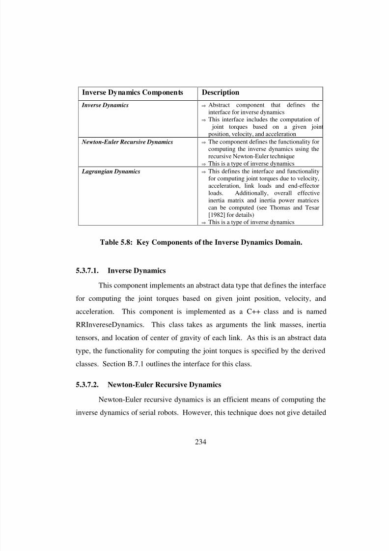
8/3/2019 Chetan Kapoor Dissertation
http://slidepdf.com/reader/full/chetan-kapoor-dissertation 258/612
234
5.3.7.1. Inverse Dynamics
This component implements an abstract data type that defines the interface
for computing the joint torques based on given joint position, velocity, and
acceleration. This component is implemented as a C++ class and is named
RRInvereseDynamics. This class takes as arguments the link masses, inertia
tensors, and location of center of gravity of each link. As this is an abstract data
type, the functionality for computing the joint torques is specified by the derived
classes. Section B.7.1 outlines the interface for this class.
5.3.7.2. Newton-Euler Recursive Dynamics
Newton-Euler recursive dynamics is an efficient means of computing the
inverse dynamics of serial robots. However, this technique does not give detailed
Inverse Dynamics Components Description
Inverse Dynamics ⇒ Abstract component that defines theinterface for inverse dynamics
⇒ This interface includes the computation of joint torques based on a given jointposition, velocity, and acceleration
Newton-Euler Recursive Dynamics ⇒ The component defines the functionality forcomputing the inverse dynamics using therecursive Newton-Euler technique
⇒ This is a type of inverse dynamics
Lagrangian Dynamics ⇒ This defines the interface and functionalityfor computing joint torques due to velocity,acceleration, link loads and end-effector
loads. Additionally, overall effectiveinertia matrix and inertia power matricescan be computed (see Thomas and Tesar[1982] for details)
⇒ This is a type of inverse dynamics
Table 5.8: Key Components of the Inverse Dynamics Domain.
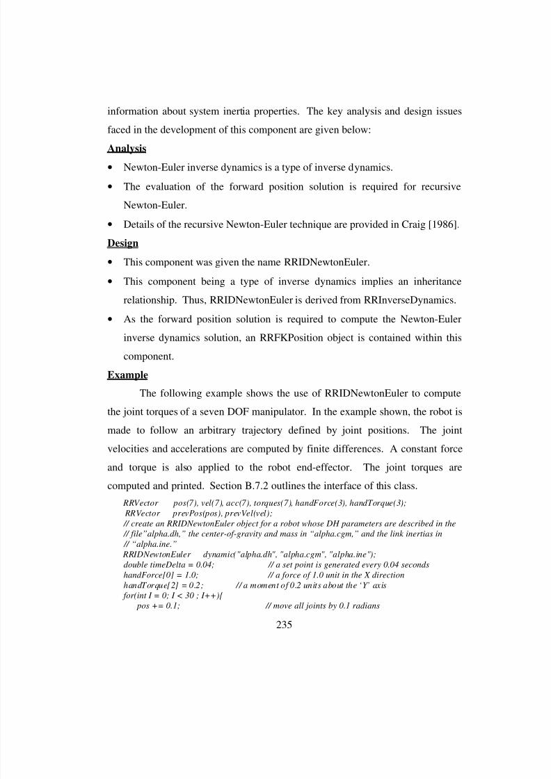
8/3/2019 Chetan Kapoor Dissertation
http://slidepdf.com/reader/full/chetan-kapoor-dissertation 259/612
235
information about system inertia properties. The key analysis and design issues
faced in the development of this component are given below:
Analysis
• Newton-Euler inverse dynamics is a type of inverse dynamics.
• The evaluation of the forward position solution is required for recursive
Newton-Euler.
• Details of the recursive Newton-Euler technique are provided in Craig [1986].
Design
• This component was given the name RRIDNewtonEuler.
• This component being a type of inverse dynamics implies an inheritance
relationship. Thus, RRIDNewtonEuler is derived from RRInverseDynamics.
• As the forward position solution is required to compute the Newton-Euler
inverse dynamics solution, an RRFKPosition object is contained within this
component.
Example
The following example shows the use of RRIDNewtonEuler to compute
the joint torques of a seven DOF manipulator. In the example shown, the robot is
made to follow an arbitrary trajectory defined by joint positions. The joint
velocities and accelerations are computed by finite differences. A constant force
and torque is also applied to the robot end-effector. The joint torques are
computed and printed. Section B.7.2 outlines the interface of this class.
RRVector pos(7), vel(7), acc(7), torques(7), handForce(3), handTorque(3);
RRVector prevPos(pos), prevVel(vel);
// create an RRIDNewtonEuler object for a robot whose DH parameters are described in the
// file”alpha.dh,” the center-of-gravity and mass in “alpha.cgm,” and the link inertias in
// “alpha.ine.” RRIDNewtonEuler dynamic("alpha.dh", "alpha.cgm", "alpha.ine");
double timeDelta = 0.04; // a set point is generated every 0.04 seconds
handForce[0] = 1.0; // a force of 1.0 unit in the X direction
handTorque[2] = 0.2; // a moment of 0.2 units about the ‘Y’ axis
for(int I = 0; I < 30 ; I++){
pos += 0.1; // move all joints by 0.1 radians
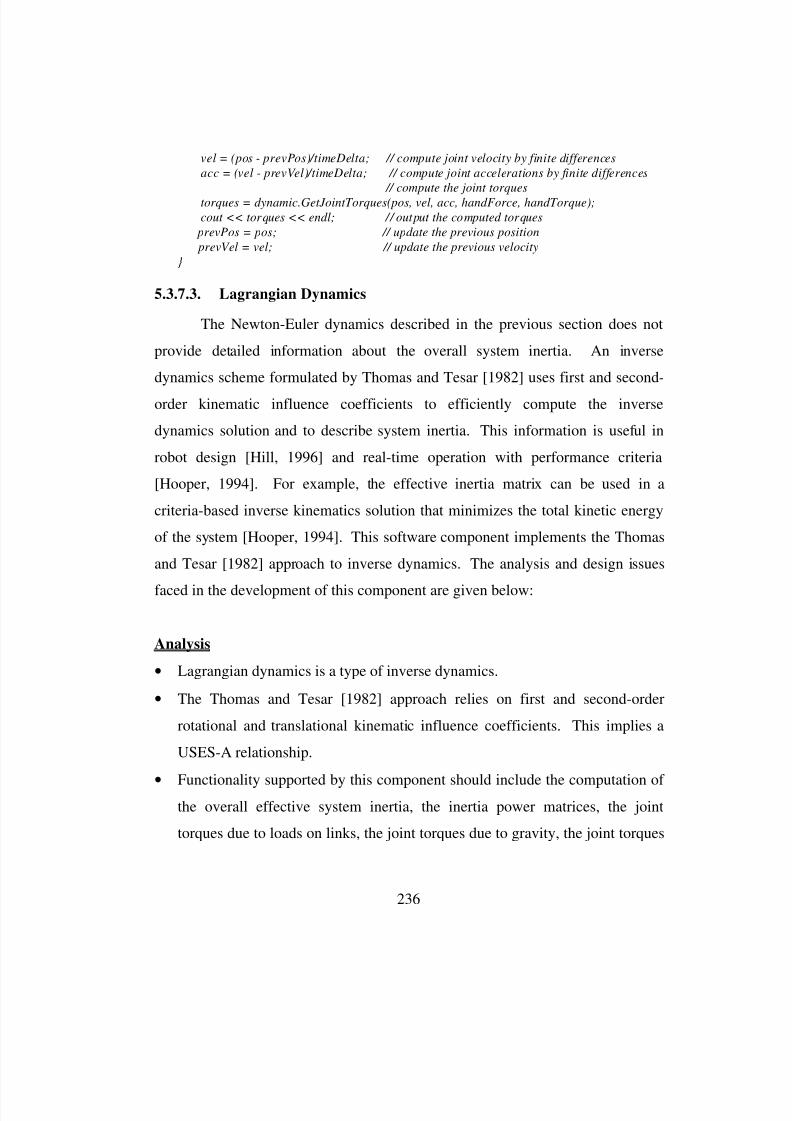
8/3/2019 Chetan Kapoor Dissertation
http://slidepdf.com/reader/full/chetan-kapoor-dissertation 260/612
236
vel = (pos - prevPos)/timeDelta; // compute joint velocity by finite differences
acc = (vel - prevVel)/timeDelta; // compute joint accelerations by finite differences
// compute the joint torques
torques = dynamic.GetJointTorques(pos, vel, acc, handForce, handTorque);
cout << torques << endl; // output the computed torques
prevPos = pos; // update the previous position
prevVel = vel; // update the previous velocity
}
5.3.7.3. Lagrangian Dynamics
The Newton-Euler dynamics described in the previous section does not
provide detailed information about the overall system inertia. An inverse
dynamics scheme formulated by Thomas and Tesar [1982] uses first and second-
order kinematic influence coefficients to efficiently compute the inverse
dynamics solution and to describe system inertia. This information is useful in
robot design [Hill, 1996] and real-time operation with performance criteria
[Hooper, 1994]. For example, the effective inertia matrix can be used in a
criteria-based inverse kinematics solution that minimizes the total kinetic energy
of the system [Hooper, 1994]. This software component implements the Thomas
and Tesar [1982] approach to inverse dynamics. The analysis and design issues
faced in the development of this component are given below:
Analysis
• Lagrangian dynamics is a type of inverse dynamics.
• The Thomas and Tesar [1982] approach relies on first and second-order
rotational and translational kinematic influence coefficients. This implies a
USES-A relationship.
•
Functionality supported by this component should include the computation of the overall effective system inertia, the inertia power matrices, the joint
torques due to loads on links, the joint torques due to gravity, the joint torques
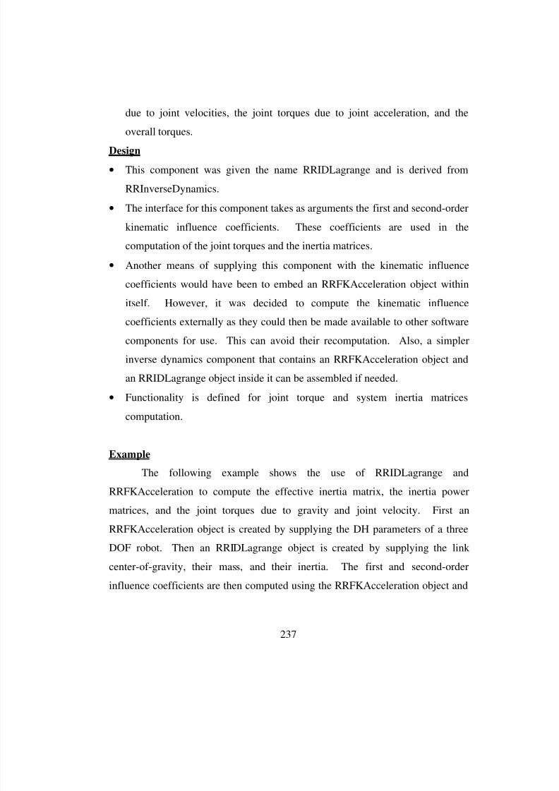
8/3/2019 Chetan Kapoor Dissertation
http://slidepdf.com/reader/full/chetan-kapoor-dissertation 261/612
237
due to joint velocities, the joint torques due to joint acceleration, and the
overall torques.
Design
• This component was given the name RRIDLagrange and is derived from
RRInverseDynamics.
• The interface for this component takes as arguments the first and second-order
kinematic influence coefficients. These coefficients are used in the
computation of the joint torques and the inertia matrices.
• Another means of supplying this component with the kinematic influence
coefficients would have been to embed an RRFKAcceleration object within
itself. However, it was decided to compute the kinematic influence
coefficients externally as they could then be made available to other software
components for use. This can avoid their recomputation. Also, a simpler
inverse dynamics component that contains an RRFKAcceleration object and
an RRIDLagrange object inside it can be assembled if needed.
• Functionality is defined for joint torque and system inertia matrices
computation.
Example
The following example shows the use of RRIDLagrange and
RRFKAcceleration to compute the effective inertia matrix, the inertia power
matrices, and the joint torques due to gravity and joint velocity. First an
RRFKAcceleration object is created by supplying the DH parameters of a three
DOF robot. Then an RRIDLagrange object is created by supplying the link
center-of-gravity, their mass, and their inertia. The first and second-order
influence coefficients are then computed using the RRFKAcceleration object and
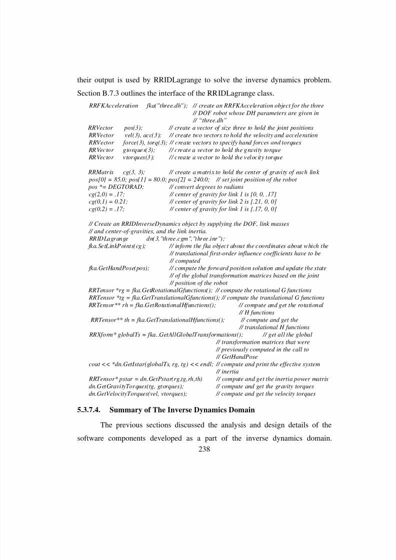
8/3/2019 Chetan Kapoor Dissertation
http://slidepdf.com/reader/full/chetan-kapoor-dissertation 262/612
238
their output is used by RRIDLagrange to solve the inverse dynamics problem.
Section B.7.3 outlines the interface of the RRIDLagrange class.
RRFKAcceleration fka("three.dh"); // create an RRFKAcceleration object for the three
// DOF robot whose DH parameters are given in
// “three.dh”
RRVector pos(3); // create a vector of size three to hold the joint positions
RRVector vel(3), acc(3); // create two vectors to hold the velocity and acceleration
RRVector force(3), torq(3); // create vectors to specify hand forces and torques
RRVector gtorques(3); // create a vector to hold the gravity torque
RRVector vtorques(3); // create a vector to hold the velocity torque
RRMatrix cg(3, 3); // create a matrix to hold the center of gravity of each link
pos[0] = 85.0; pos[1] = 80.0; pos[2] = 240.0; // set joint position of the robot
pos *= DEGTORAD; // convert degrees to radians
cg(2,0) = .17; // center of gravity for link 1 is [0, 0, .17]cg(0,1) = 0.21; // center of gravity for link 2 is [.21, 0, 0]
cg(0,2) = .17; // center of gravity for link 1 is [.17, 0, 0]
// Create an RRIDInverseDynamics object by supplying the DOF, link masses
// and center-of-gravities, and the link inertia.
RRIDLagrange dn(3,"three.cgm","three.inr");
fka.SetLinkPoints(cg); // inform the fka object about the coordinates about which the
// translational first-order influence coefficients have to be
// computed
fka.GetHandPose(pos); // compute the forward position solution and update the state
// of the global transformation matrices based on the joint
// position of the robot
RRTensor *rg = fka.GetRotationalGfunctions(); // compute the rotational G functions
RRTensor *tg = fka.GetTranslationalGfunctions(); // compute the translational G functions
RRTensor** rh = fka.GetRotationalHfunctions(); // compute and get the rotational
// H functions
RRTensor** th = fka.GetTranslationalHfunctions(); // compute and get the
// translational H functions
RRXform* globalTs = fka..GetAllGlobalTransformations(); // get all the global
// transformation matrices that were
// previously computed in the call to
// GetHandPose
cout << *dn.GetIstar(globalTs, rg, tg) << endl; // compute and print the effective system
// inertia
RRTensor* pstar = dn.GetPstar(rg,tg,rh,th) // compute and get the inertia power matrix
dn.GetGravityTorques(tg, gtorques); // compute and get the gravity torques
dn.GetVelocityTorques(vel, vtorques); // compute and get the velocity torques
5.3.7.4. Summary of The Inverse Dynamics Domain
The previous sections discussed the analysis and design details of the
software components developed as a part of the inverse dynamics domain.
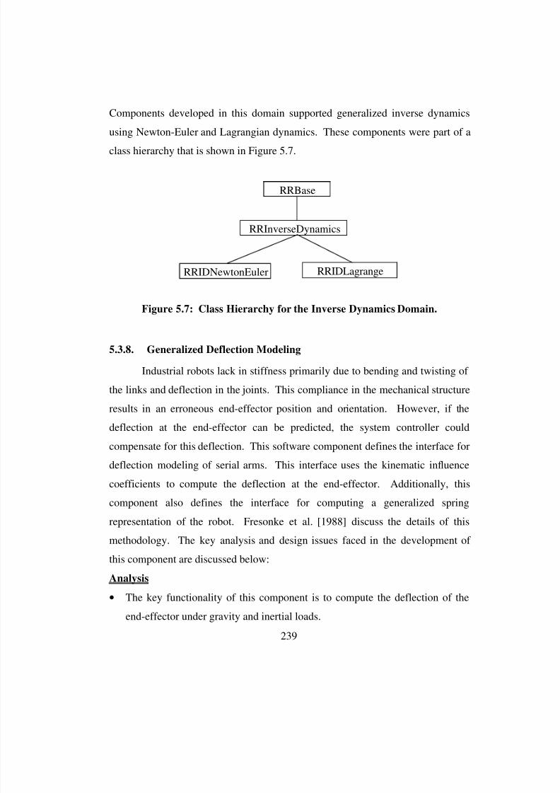
8/3/2019 Chetan Kapoor Dissertation
http://slidepdf.com/reader/full/chetan-kapoor-dissertation 263/612
239
Components developed in this domain supported generalized inverse dynamics
using Newton-Euler and Lagrangian dynamics. These components were part of a
class hierarchy that is shown in Figure 5.7.
5.3.8. Generalized Deflection Modeling
Industrial robots lack in stiffness primarily due to bending and twisting of
the links and deflection in the joints. This compliance in the mechanical structure
results in an erroneous end-effector position and orientation. However, if the
deflection at the end-effector can be predicted, the system controller could
compensate for this deflection. This software component defines the interface for
deflection modeling of serial arms. This interface uses the kinematic influence
coefficients to compute the deflection at the end-effector. Additionally, this
component also defines the interface for computing a generalized spring
representation of the robot. Fresonke et al. [1988] discuss the details of this
methodology. The key analysis and design issues faced in the development of
this component are discussed below:
Analysis
• The key functionality of this component is to compute the deflection of the
end-effector under gravity and inertial loads.
RRInverseDynamics
RRIDNewtonEulerRRIDLagrange
RRBase
Figure 5.7: Class Hierarchy for the Inverse Dynamics Domain.
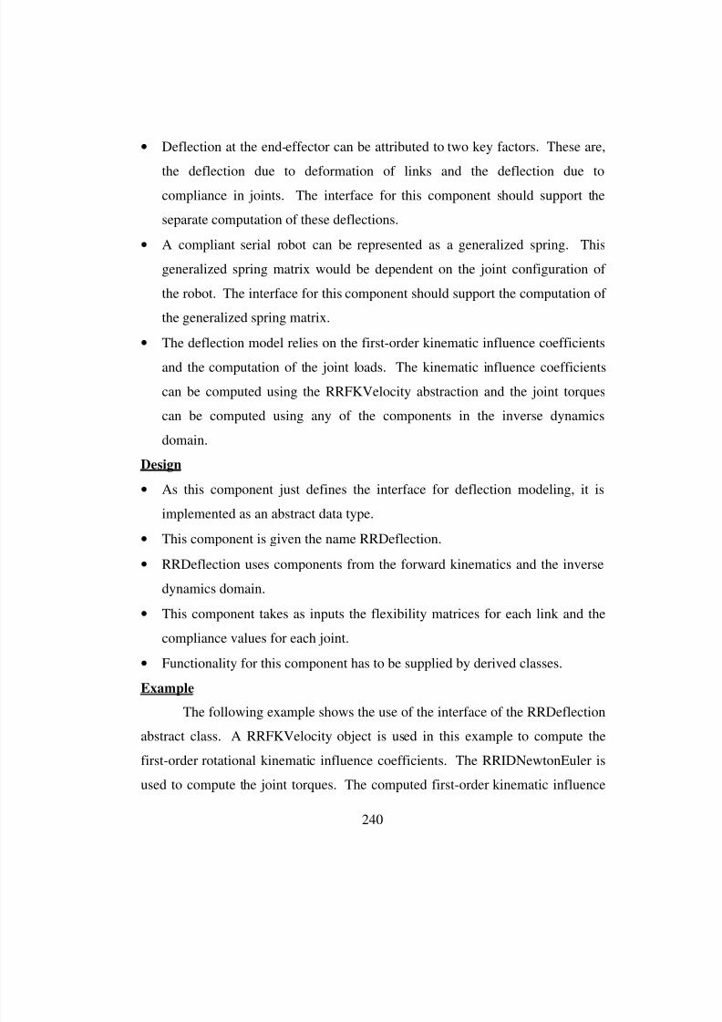
8/3/2019 Chetan Kapoor Dissertation
http://slidepdf.com/reader/full/chetan-kapoor-dissertation 264/612
240
• Deflection at the end-effector can be attributed to two key factors. These are,
the deflection due to deformation of links and the deflection due to
compliance in joints. The interface for this component should support the
separate computation of these deflections.
• A compliant serial robot can be represented as a generalized spring. This
generalized spring matrix would be dependent on the joint configuration of
the robot. The interface for this component should support the computation of
the generalized spring matrix.
• The deflection model relies on the first-order kinematic influence coefficients
and the computation of the joint loads. The kinematic influence coefficients
can be computed using the RRFKVelocity abstraction and the joint torques
can be computed using any of the components in the inverse dynamics
domain.
Design
• As this component just defines the interface for deflection modeling, it is
implemented as an abstract data type.
• This component is given the name RRDeflection.
• RRDeflection uses components from the forward kinematics and the inverse
dynamics domain.
• This component takes as inputs the flexibility matrices for each link and the
compliance values for each joint.
• Functionality for this component has to be supplied by derived classes.
Example
The following example shows the use of the interface of the RRDeflectionabstract class. A RRFKVelocity object is used in this example to compute the
first-order rotational kinematic influence coefficients. The RRIDNewtonEuler is
used to compute the joint torques. The computed first-order kinematic influence

8/3/2019 Chetan Kapoor Dissertation
http://slidepdf.com/reader/full/chetan-kapoor-dissertation 265/612
241
coefficients and the joint torques are then used to compute the deflection in the
links and the actuators respectively. Section B.8.1 outlines the interface of the
RRDeflection class.
RRFKVelocity fkv("three.dh"); // create an RRFKVelocity object for the three
// DOF robot whose DH parameters are given in
// “three.dh”
// create an RRIDNewtonEuler object for a robot whose DH parameters are described in the
// file”three.dh,” the center-of-gravity and mass in “three.cgm,” and the link inertias in
// “three.ine.”
RRIDNewtonEuler dynamic("three.dh", "three.cgm", "three.ine");
// create a RRDeflection object by specifying the degrees-of-freedom, the link flexibility
// matrices and the joint stiffness
RRDeflectiondeflect(fkv.GetDOF(), “linkFlex.dat”, “jointFlex.dat”);
RRVector linkDeflect(3); // create a vector for holding link deflections
RRVector jointDeflect(3); // create a vector for holding joint deflections
double timeDelta = 0.04; // a set point is generated every 0.04 seconds
handForce[0] = 1.0; // a force of 1.0 unit in the ‘X’ direction
handTorque[2] = 0.2; // a moment of 0.2 units about the ‘Y’ axis
for(int I = 0; I < 30 ; I++){
pos += 0.1; // move all joints by 0.1 radians
vel = (pos - prevPos)/timeDelta; // compute joint velocity by finite differences
acc = (vel - prevVel)/timeDelta; // compute joint accelerations by finite differences
// compute the joint torques
torques = dynamic.GetJointTorques(pos, vel, acc, handForce, handTorque);
fkv.GetHandPose(pos); // compute the forward position solution and update the state
// of the global transformation matrices based on the joint
// position of the robot // compute the rotational G functions
RRTensor *rg = fkv.GetRotationalGfunctions();
deflect.GetDeflectionDueToLinks(rg, linkDeflect); // compute deflection due to links
deflect.GetLocalJointDeflection(torques, jointDeflect); // deflection due to joints
}
5.3.8.1. Summary of The Generalized Deflection Modeling Domain
The previous section discussed the analysis and design details of the
component developed as a part of the deflection modeling domain. The class
hierarchy for the component developed in this domain is shown in Figure 5.8.
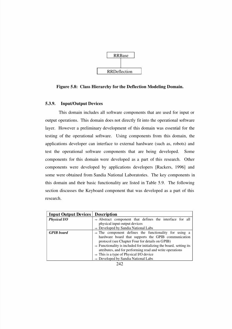
8/3/2019 Chetan Kapoor Dissertation
http://slidepdf.com/reader/full/chetan-kapoor-dissertation 266/612
242
5.3.9. Input/Output Devices
This domain includes all software components that are used for input or
output operations. This domain does not directly fit into the operational software
layer. However a preliminary development of this domain was essential for the
testing of the operational software. Using components from this domain, the
applications developer can interface to external hardware (such as, robots) and
test the operational software components that are being developed. Some
components for this domain were developed as a part of this research. Other
components were developed by applications developers [Rackers, 1996] and
some were obtained from Sandia National Laboratories. The key components in
this domain and their basic functionality are listed in Table 5.9. The following
section discusses the Keyboard component that was developed as a part of this
research.
Input Output Devices Description Physical I/O ⇒ Abstract component that defines the interface for all
physical input output devices⇒ Developed by Sandia National Labs
GPIB board ⇒ The component defines the functionality for using ahardware board that supports the GPIB communicationprotocol (see Chapter Four for details on GPIB)
⇒ Functionality is included for initializing the board, setting itsattributes, and for performing read and write operations
⇒ This is a type of Physical I/O device⇒ Developed by Sandia National Labs
RRDeflection
RRBase
Figure 5.8: Class Hierarchy for the Deflection Modeling Domain.
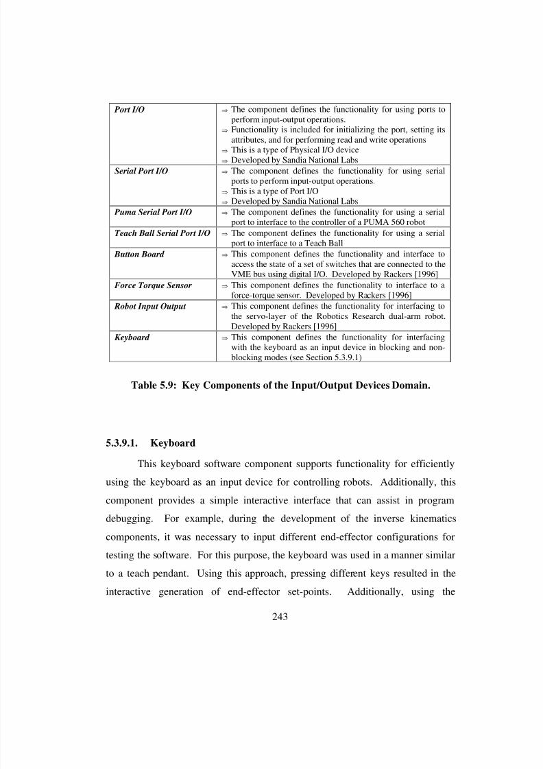
8/3/2019 Chetan Kapoor Dissertation
http://slidepdf.com/reader/full/chetan-kapoor-dissertation 267/612
243
Port I/O ⇒ The component defines the functionality for using ports toperform input-output operations.
⇒ Functionality is included for initializing the port, setting itsattributes, and for performing read and write operations
⇒ This is a type of Physical I/O device⇒ Developed by Sandia National Labs
Serial Port I/O ⇒ The component defines the functionality for using serialports to perform input-output operations.
⇒ This is a type of Port I/O⇒ Developed by Sandia National Labs
Puma Serial Port I/O ⇒ The component defines the functionality for using a serialport to interface to the controller of a PUMA 560 robot
Teach Ball Serial Port I/O ⇒ The component defines the functionality for using a serialport to interface to a Teach Ball
Button Board ⇒ This component defines the functionality and interface toaccess the state of a set of switches that are connected to theVME bus using digital I/O. Developed by Rackers [1996]
Force Torque Sensor ⇒ This component defines the functionality to interface to aforce-torque sensor. Developed by Rackers [1996]
Robot Input Output ⇒ This component defines the functionality for interfacing tothe servo-layer of the Robotics Research dual-arm robot.Developed by Rackers [1996]
Keyboard ⇒ This component defines the functionality for interfacingwith the keyboard as an input device in blocking and non-blocking modes (see Section 5.3.9.1)
Table 5.9: Key Components of the Input/Output Devices Domain.
5.3.9.1. Keyboard
This keyboard software component supports functionality for efficiently
using the keyboard as an input device for controlling robots. Additionally, this
component provides a simple interactive interface that can assist in program
debugging. For example, during the development of the inverse kinematics
components, it was necessary to input different end-effector configurations fortesting the software. For this purpose, the keyboard was used in a manner similar
to a teach pendant. Using this approach, pressing different keys resulted in the
interactive generation of end-effector set-points. Additionally, using the
8/3/2019 Chetan Kapoor Dissertation
http://slidepdf.com/reader/full/chetan-kapoor-dissertation 268/612
244
keyboard, a physical robot could be controlled similarly. The key analysis and
design issues faced in the development of this component are discussed below:
Analysis
• The key functionality of this component is to provide the ability to test the
state of a key. That is, whether a key is pressed or not.
• The user should be able to test the state of a key in blocking and non-blocking
mode. Under blocking mode, the program waits until a key is pressed. Under
non-blocking mode, the program just polls the keyboard and checks the state
of the keys (for details see [WindRiver Systems, VxWorks Programmer’s
Guide]).
• The keyboard has to be reconfigured for non-canonical character processing.
Canonical character processing relies on specific formats for character input.
This is the default mode. For example, under canonical processing, a carriage
return has to be input after a character is input. Under non-canonical (also
called raw mode), only a character has to be input. The input character does
not have to be followed by a carriage return (for details on canonical and raw
character processing see [WindRiver Systems, VxWorks Programmer’s
Guide]).
Design
• This component was given the name RRKeyboard and was derived from
RRBase.
• It supports the functionality to set the keyboard to non-blocking mode and the
character processing to raw mode.
•
The software implementation for this component is specific to the operatingsystem. Currently, VxWorks, UNIX, and Windows NT are supported.
Example

8/3/2019 Chetan Kapoor Dissertation
http://slidepdf.com/reader/full/chetan-kapoor-dissertation 269/612
245
The following example shows the use of the keyboard in blocking mode
with raw character processing. The program loops and prints out the value of the
key that was pressed. The program quits when the escape key is pressed. Section
B.9.1 outlines the interface of the RRKeyboard class.
#define ESCAPE 27 // escape key is ASCII code 27
RRKeyboard keyboard(RRKeyboard::BLOCK); // create an RRKeyboard object that puts the
// keyboard in a blocking mode
char key = 0; // the pressed key will be stored in this
while(key != ESCAPE){ // loop till the escape key is pressed
key = keyboard.GetKey(); // get the value of the key that is pressed
cout << “Key pressed = “ << key << endl; // print the key that was pressed
}
5.3.10. Controllers
This domain was developed to facilitate the integration of manual
controllers into the software testing environment. Again, this domain does not fit
directly into the operational software layer. However, the development of this
layer assisted in testing the operational software components in a manual
controller environment. Two key components were developed under this domain.
These were an abstract component for manual controllers and a component to
support the TeachBall. Software for other manual controllers like the six DOF
TOS arm and the six DOF Perforce controller has also been developed [Peterson,
1996]. However, the software for these systems is still in development and test
stages and has not been integrated into this framework. Table 5.10 lists the key
components in the controller domain. Further, the analysis and design issues
faced in the development of the TeachBall software component are discussed.

8/3/2019 Chetan Kapoor Dissertation
http://slidepdf.com/reader/full/chetan-kapoor-dissertation 270/612
246
5.3.10.1. TeachBall
The TeachBall is a six DOF input device. Additionally, the TeachBall has
eight buttons that can be used for entering additional information. The TeachBall
can be connected to any computer that supports an RS-232 based serial port. The
software component for the TeachBall provides a general purpose interface that
can be used for any six DOF input device. The key analysis and design issues
faced in the development of this component are discussed below:
Analysis
• The key functionality of this component is to interface with the TeachBall
hardware and read its state.
• As the TeachBall uses a serial port, a serial port object is contained inside this
component.
• The user should be able to supply this component with a vector of hand
positions and orientations, and this component should be able to update this
vector based on the TeachBall movement.
Design
• This component was given the name RRTeachBall and was derived fromRRController.
• RRTeachBall contains an RRTeachBallSerialPort object.
Controllers DescriptionController ⇒ Abstract component that defines a general purpose interface
for manual controllers
TeachBall ⇒ The component defines the functionality for using aTeachBall as a manual controller
Table 5.10: Key Components of the Input Output Devices Domain.

8/3/2019 Chetan Kapoor Dissertation
http://slidepdf.com/reader/full/chetan-kapoor-dissertation 271/612
247
• Functionality is provided to read the position of the TeachBall and also to
read the state of the buttons.
Example
The following example shows the use of the RRTeachBall manual
controller class to update a vector that specifies the end-effector location. The
updated end-effector can be input into an inverse kinematics object and the
resulting joint solution can be used to control a robot. First an RRHandPose
object is created to hold the robot hand position and orientation. Then an
RRTeachBall object is created by specifying the RRHandPose vector it will
update and the number of the serial port to which the TeachBall is connected.
Resulting this, the button status and the movements of the TeachBall are
continuously read until the first button is pressed. Section B.10.2 outlines the
interface of the RRTeachBall class.
RRHandPoserobotHand; // create a vector for holding end-effector position
// and orientation
robotHand.X() = 10.0; // set ‘X’ coordinate to 10.0
robotHand.Y() = 15.0; // set ‘Y’ coordinate to 15.0
robotHand.Z() = -5.0; // set ‘Z’ coordinate to -5.0
robotHand.Roll() = 0.05; // set Roll angle to 0.05
robotHand.Pitch() = 0.01; // set Pitch angle to 0.01
robotHand.Yaw() = -0.02; // set Yaw angle to -0.02
RRTeachBall tb(1, robotHand); // create an RRTeachBall object that uses
// serial port 1
if(!tb.Initialize()){ // initialize TeachBall and check for error
cout << DisplayError(“Initialize on TeachBall”);
}
int buttons[8]; // create an integer array for holding buttons status
tb.GetButtonStatus(buttons); // update status of the buttons from the TeachBall
while(!buttons[0]){ // loop till button 1 is pressed on the TeachBall
tb.GetCurrentHand(robotHand, buttons); // update hand and button status
cout << “Current Hand = “ << robotHand << endl; // print the current hand
}
5.3.11. Utility Components
This domain was established to support the development of the
operational software components proposed in this research. These included error

8/3/2019 Chetan Kapoor Dissertation
http://slidepdf.com/reader/full/chetan-kapoor-dissertation 272/612
248
handling, timing, and character string encapsulation. These components and their
key functionality is outlined in Table 5.11 and details of the Timer component are
discussed in the following section.
5.3.11.1. Timer
This component encapsulates a stop-watch and is used for program
timing. Functionality is provided to start the timer, stop the timer, and to compute
the elapsed time. This component is implemented as a C++ class named
RRTimer and is derived from RRBase. Section B.11.1 outlines the interface of
the RRTimer class. An example use of the RRTimer class is shown below. In
this example, two RRTimer objects are created. One of these is used to measure
the timing of an outer for loop. The other one measures the timing of an inner for
loop. The example shows that an RRTimer object can be started and stopped
similar to a stop-watch.
double number = 1.0;
RRTimer timerA, timerB; // create two timers for program timing
timerA.Start(); // start timerA. This timer will measure
for(int I = 0; I < 10; I++){ // the elapsed time for the outer loop
timerB.Start(); // start timerB. This timer will measure
for(int j = 0; j < 3000; j++){ // the elapsed time for the inner loopnumber /= 1.1; // take up some time
}
timerB.Stop(); // stop timerB and print out the elapsed time
cout << “Elapsed time for inner loop = “ << timerB.ElapsedTime() << endl;
}
timerA.Stop(); // stop timerA and print out the elapsed time
Utility Components Description Error Handling ⇒ Sub-routines for displaying error messages
⇒ Sub-routines for displaying debugging information
String ⇒ Encapsulates a character array
Timer ⇒ Encapsulates a stop-watch⇒ Useful in program timing
Table 5.11: Key Components of the Utility Domain.

8/3/2019 Chetan Kapoor Dissertation
http://slidepdf.com/reader/full/chetan-kapoor-dissertation 273/612
249
cout << “Elapsed time for outer loop = “ << timerA.ElapsedTime() << endl;
5.3.12. Communication Components
This domain was developed to facilitate the testing of the operational
software components that were developed as a part of this research. As discussed
in Chapter Two, the operational software layer does not include software for
interfacing with external hardware or for communication with other computers.
This software is essentially a part of the lower-most layer, that is, the real-time
control layer. However, to test the operational software components, it was
necessary to develop a rudimentary real-time and hardware interfacing software
architecture. Also, as discussed in Chapter Four, manual controller integration
was supported as a part of this research. This allowed for testing the operational
software components in a manual controller environment. Also, a graphical
simulation environment had to be supported for testing and development of the
operational software. The communications domain was developed to provide a
means of integrating the operational software components with a simulation
environment, the manual controllers, and robotic hardware. Transmission Control
Protocol (TCP) sockets and Ethernet were used for the communications (see
Chapter Four for more details). The functionality of TCP sockets was
encapsulated in three key components (the reader should refer to Brain [1994] for
details on TCP sockets). These are outlined in Table 5.12 and are discussed
below:
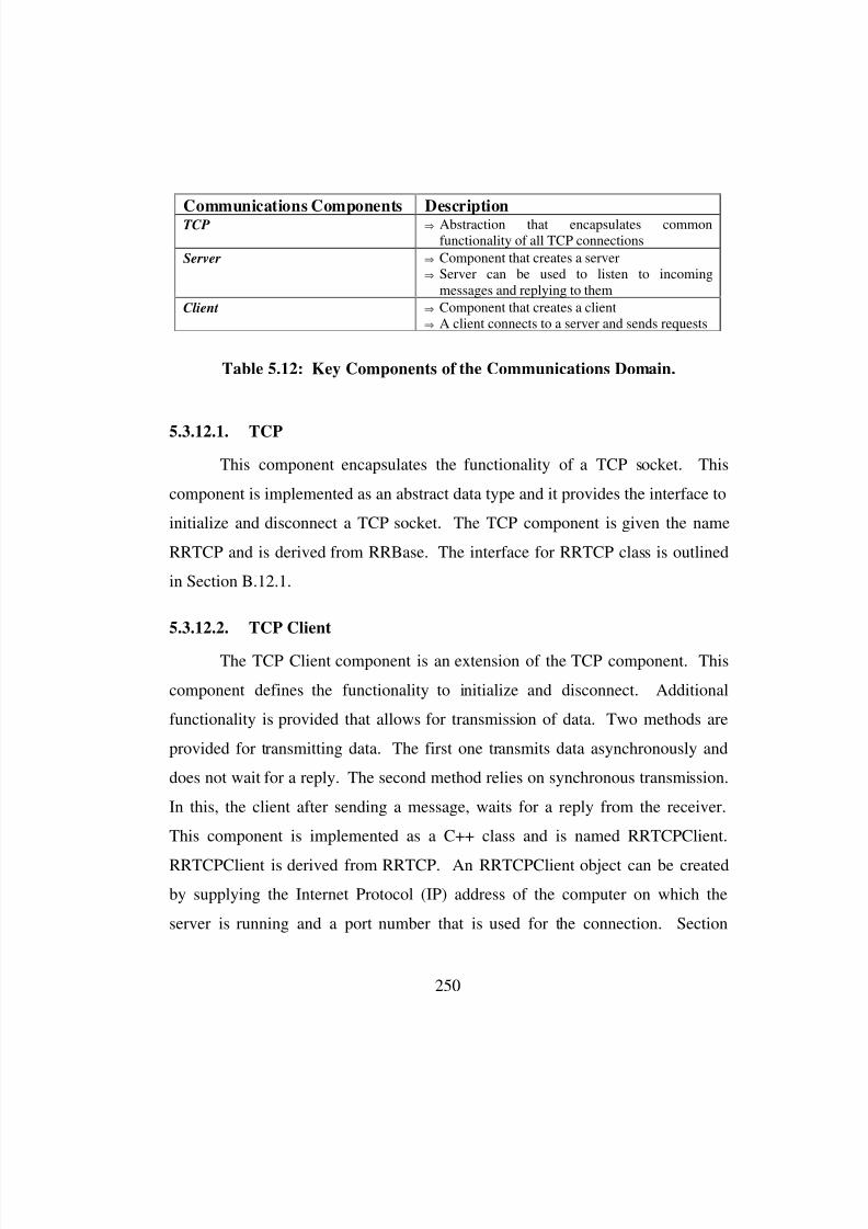
8/3/2019 Chetan Kapoor Dissertation
http://slidepdf.com/reader/full/chetan-kapoor-dissertation 274/612
250
5.3.12.1. TCP
This component encapsulates the functionality of a TCP socket. This
component is implemented as an abstract data type and it provides the interface to
initialize and disconnect a TCP socket. The TCP component is given the name
RRTCP and is derived from RRBase. The interface for RRTCP class is outlined
in Section B.12.1.
5.3.12.2. TCP Client
The TCP Client component is an extension of the TCP component. This
component defines the functionality to initialize and disconnect. Additional
functionality is provided that allows for transmission of data. Two methods are
provided for transmitting data. The first one transmits data asynchronously and
does not wait for a reply. The second method relies on synchronous transmission.
In this, the client after sending a message, waits for a reply from the receiver.
This component is implemented as a C++ class and is named RRTCPClient.
RRTCPClient is derived from RRTCP. An RRTCPClient object can be created
by supplying the Internet Protocol (IP) address of the computer on which the
server is running and a port number that is used for the connection. Section
Communications Components DescriptionTCP ⇒ Abstraction that encapsulates common
functionality of all TCP connections
Server ⇒ Component that creates a server⇒ Server can be used to listen to incoming
messages and replying to them
Client ⇒ Component that creates a client⇒ A client connects to a server and sends requests
Table 5.12: Key Components of the Communications Domain.

8/3/2019 Chetan Kapoor Dissertation
http://slidepdf.com/reader/full/chetan-kapoor-dissertation 275/612
251
B.12.2 outlines the interface of the RRTCPClient class. Given below is an
example use of the RRTCPClient class.
#define PORT 66556 // specify the port number to be used for the connection
#define SERVER_IP “129.164.123.234” // specify the IP address of the server
char toSend[] = “hello world”; // specify the string to send to the server
RRTCPClient client(SERVER_IP, PORT); // create an RRTCPClient object
if(!client.Initialize()){ // make the client connect to the server
cout << “Server on “ << SERVER_IP << “ is not running” << endl;
return;
}
client.Transmit(toSend, strlen(toSend); // send the message to the server
5.3.12.3. TCP Server
The TCP Server component is an extension of the TCP component. This
component defines the functionality to initialize and disconnect. Additional
functionality is provided that allows for receiving a message from a client and
replying to it. This component is implemented as a C++ class and is named
RRTCPServer. RRTCPServer is derived from RRTCP. An RRTCPServer object
can be created by supplying the port number that will be used by the client to
communicate. It should be noted that a server has to be running before a client
can connect and transmit data to it. Section B.12.3 outlines the interface of the
RRTCPServer class. Given below is an example use of the RRTCPServer class.
In this example, an RRTCPServer object is created and then initialized. During
initialization this object waits for a client to connect. Once connected, this object
receives data from the client and sends a reply back to the client.
#define PORT 66556 // specify the port number to be used for the connection
char recvString[20]; // character array in which the message is received
char reply[] = “acknowledge”; // specify the reply to the client
RRTCPServer server( PORT); // create an RRTCPServer object
server.Initialize(); // make the server wait for the client to connect
server.Receive(recvString, 20); // receive the message from the client server.Reply(reply, strlen(reply)); // send a reply back to the client
5.3.12.4. Summary of the Communications Domain

8/3/2019 Chetan Kapoor Dissertation
http://slidepdf.com/reader/full/chetan-kapoor-dissertation 276/612
252
The previous sections discussed the analysis and design details of the
software components developed as a part of the communications domain.
Components developed in this domain supported TCP sockets based
communications. These components were part of a class hierarchy that is shown
in Figure 5.9.
5.3.13. Other Components
This domain holds all other software components that facilitate software
development. These components do not directly fit into the advanced robotics
domain but are necessary for program development. The components for this
domain were not developed as a part of this research. These components were
purchased from commercial vendors (see Table 5.13). The software for these
components came in the form of a class library (similar to what is being
developed in this research). The key sub-domains and components supported in
this domain are listed in Table 5.13.
RRTCP
RRTCPServer RRTCPClient
RRBase
Figure 5.9: Class Hierarchy for the Communications Domain.
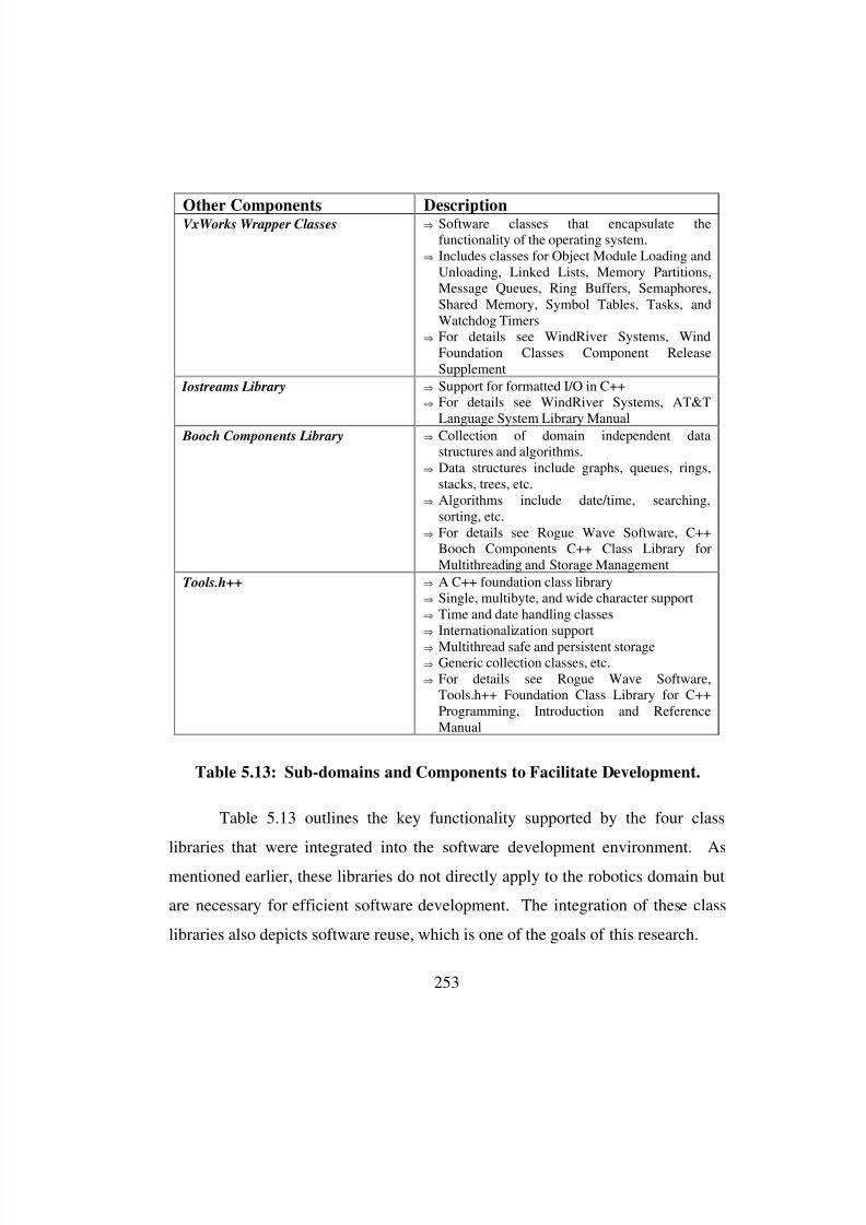
8/3/2019 Chetan Kapoor Dissertation
http://slidepdf.com/reader/full/chetan-kapoor-dissertation 277/612
253
Table 5.13 outlines the key functionality supported by the four class
libraries that were integrated into the software development environment. As
mentioned earlier, these libraries do not directly apply to the robotics domain but
are necessary for efficient software development. The integration of these class
libraries also depicts software reuse, which is one of the goals of this research.
Other Components DescriptionVxWorks Wrapper Classes ⇒ Software classes that encapsulate the
functionality of the operating system.⇒ Includes classes for Object Module Loading and
Unloading, Linked Lists, Memory Partitions,Message Queues, Ring Buffers, Semaphores,Shared Memory, Symbol Tables, Tasks, andWatchdog Timers
⇒ For details see WindRiver Systems, WindFoundation Classes Component ReleaseSupplement
Iostreams Library ⇒ Support for formatted I/O in C++⇒ For details see WindRiver Systems, AT&T
Language System Library Manual
Booch Components Library ⇒ Collection of domain independent datastructures and algorithms.
⇒ Data structures include graphs, queues, rings,stacks, trees, etc.
⇒ Algorithms include date/time, searching,sorting, etc.
⇒ For details see Rogue Wave Software, C++Booch Components C++ Class Library forMultithreading and Storage Management
Tools.h++ ⇒ A C++ foundation class library⇒ Single, multibyte, and wide character support⇒ Time and date handling classes⇒ Internationalization support
⇒ Multithread safe and persistent storage⇒ Generic collection classes, etc.⇒ For details see Rogue Wave Software,
Tools.h++ Foundation Class Library for C++Programming, Introduction and ReferenceManual
Table 5.13: Sub-domains and Components to Facilitate Development.
8/3/2019 Chetan Kapoor Dissertation
http://slidepdf.com/reader/full/chetan-kapoor-dissertation 278/612
254
5.4. Summary
This chapter presented the core of this research, that is, the abstraction (or
component) development process. First, the three basic steps of object-oriented
design were discussed. These were, analysis, design, and implementation.
Further on, an analysis of the domain of advanced robotics led to the
identification of sub-domains. Additional domains were added to facilitate
software development and testing. The next step was a detailed analysis of the
sub-domains and the identification of the software components that were a part of
the domain. These components were then analyzed independently and their
functionality, attributes, and relationships defined. After completion of the
analysis of each component, the implementation level specifications were
generated in the design phase. For all major components discussed in this
chapter, an example use was provided. The reader was asked to refer to
Appendix B for details on the interface and use of each component.

8/3/2019 Chetan Kapoor Dissertation
http://slidepdf.com/reader/full/chetan-kapoor-dissertation 279/612
255
Chapter Six
6. Demonstrations and Experiments
6.1. Introduction
The key goal of this research was to develop an operational software
architecture (OSCAR) that had the following characteristics:
• Support for advanced robotics. Advanced robotics includes:
a. Redundant robot arms
b.
Generalized kinematicsc. Criteria-based decision making
d. Generalized dynamics
e. Deflection modeling
f. Fault-tolerance
• Completely general software architecture. Should apply to any serial arm.
• Applicability to real-time control.
• Applicability to simulation.
• Exhibit reuse through extensibility.
• Support rapid-prototyping.
• Cut down control program development time by 50%.
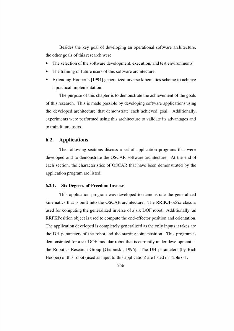
8/3/2019 Chetan Kapoor Dissertation
http://slidepdf.com/reader/full/chetan-kapoor-dissertation 280/612
256
Besides the key goal of developing an operational software architecture,
the other goals of this research were:
• The selection of the software development, execution, and test environments.
• The training of future users of this software architecture.
• Extending Hooper’s [1994] generalized inverse kinematics scheme to achieve
a practical implementation.
The purpose of this chapter is to demonstrate the achievement of the goals
of this research. This is made possible by developing software applications using
the developed architecture that demonstrate each achieved goal. Additionally,
experiments were performed using this architecture to validate its advantages and
to train future users.
6.2. Applications
The following sections discuss a set of application programs that were
developed and to demonstrate the OSCAR software architecture. At the end of
each section, the characteristics of OSCAR that have been demonstrated by the
application program are listed.
6.2.1. Six Degrees-of-Freedom Inverse
This application program was developed to demonstrate the generalized
kinematics that is built into the OSCAR architecture. The RRIKJForSix class is
used for computing the generalized inverse of a six DOF robot. Additionally, an
RRFKPosition object is used to compute the end-effector position and orientation.
The application developed is completely generalized as the only inputs it takes are
the DH parameters of the robot and the starting joint position. This program is
demonstrated for a six DOF modular robot that is currently under development at
the Robotics Research Group [Grupinski, 1996]. The DH parameters (by Rich
Hooper) of this robot (used as input to this application) are listed in Table 6.1.
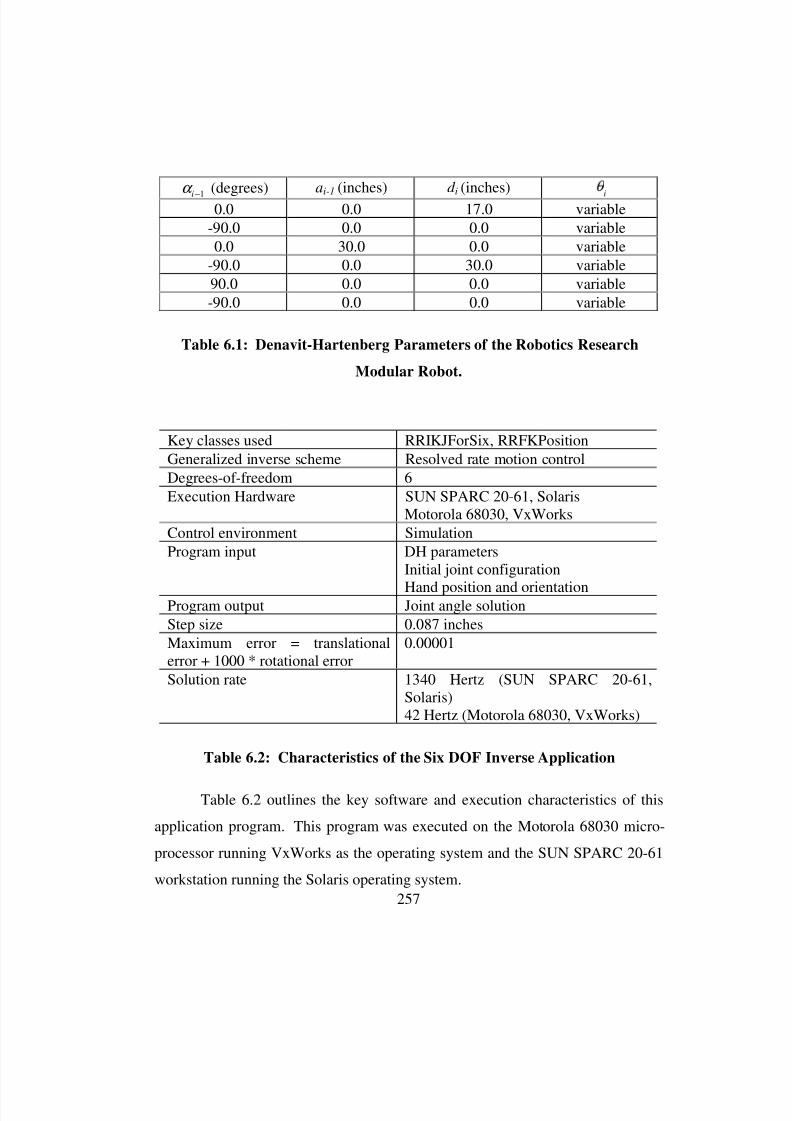
8/3/2019 Chetan Kapoor Dissertation
http://slidepdf.com/reader/full/chetan-kapoor-dissertation 281/612
257
Table 6.2 outlines the key software and execution characteristics of this
application program. This program was executed on the Motorola 68030 micro-
processor running VxWorks as the operating system and the SUN SPARC 20-61
workstation running the Solaris operating system.
α i−1
(degrees) ai-1
(inches) d i(inches)
i
0.0 0.0 17.0 variable
-90.0 0.0 0.0 variable
0.0 30.0 0.0 variable
-90.0 0.0 30.0 variable
90.0 0.0 0.0 variable
-90.0 0.0 0.0 variable
Table 6.1: Denavit-Hartenberg Parameters of the Robotics Research
Modular Robot.
Key classes used RRIKJForSix, RRFKPosition
Generalized inverse scheme Resolved rate motion control
Degrees-of-freedom 6
Execution Hardware SUN SPARC 20-61, SolarisMotorola 68030, VxWorks
Control environment Simulation
Program input DH parametersInitial joint configuration
Hand position and orientationProgram output Joint angle solution
Step size 0.087 inches
Maximum error = translationalerror + 1000 * rotational error
0.00001
Solution rate 1340 Hertz (SUN SPARC 20-61,Solaris)42 Hertz (Motorola 68030, VxWorks)
Table 6.2: Characteristics of the Six DOF Inverse Application

8/3/2019 Chetan Kapoor Dissertation
http://slidepdf.com/reader/full/chetan-kapoor-dissertation 282/612
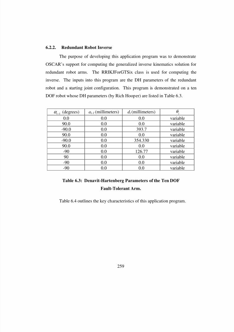
8/3/2019 Chetan Kapoor Dissertation
http://slidepdf.com/reader/full/chetan-kapoor-dissertation 283/612
259
6.2.2. Redundant Robot Inverse
The purpose of developing this application program was to demonstrateOSCAR’s support for computing the generalized inverse kinematics solution for
redundant robot arms. The RRIKJForGTSix class is used for computing the
inverse. The inputs into this program are the DH parameters of the redundant
robot and a starting joint configuration. This program is demonstrated on a ten
DOF robot whose DH parameters (by Rich Hooper) are listed in Table 6.3.
Table 6.4 outlines the key characteristics of this application program.
α i−1 (degrees) ai-1 (millimeters) d i (millimeters) i
0.0 0.0 0.0 variable
90.0 0.0 0.0 variable
-90.0 0.0 393.7 variable
90.0 0.0 0.0 variable
-90.0 0.0 354.330 variable
90.0 0.0 0.0 variable
-90 0.0 126.77 variable
90 0.0 0.0 variable
-90 0.0 0.0 variable
-90 0.0 0.0 variable
Table 6.3: Denavit-Hartenberg Parameters of the Ten DOF
Fault-Tolerant Arm.
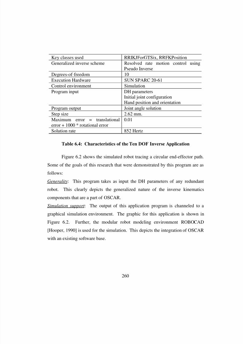
8/3/2019 Chetan Kapoor Dissertation
http://slidepdf.com/reader/full/chetan-kapoor-dissertation 284/612
260
Figure 6.2 shows the simulated robot tracing a circular end-effector path.
Some of the goals of this research that were demonstrated by this program are as
follows:
Generality: This program takes as input the DH parameters of any redundant
robot. This clearly depicts the generalized nature of the inverse kinematics
components that are a part of OSCAR.
Simulation support : The output of this application program is channeled to a
graphical simulation environment. The graphic for this application is shown in
Figure 6.2. Further, the modular robot modeling environment ROBOCAD
[Hooper, 1990] is used for the simulation. This depicts the integration of OSCAR
with an existing software base.
Key classes used RRIKJForGTSix, RRFKPosition
Generalized inverse scheme Resolved rate motion control usingPseudo Inverse
Degrees-of-freedom 10
Execution Hardware SUN SPARC 20-61
Control environment Simulation
Program input DH parametersInitial joint configurationHand position and orientation
Program output Joint angle solution
Step size 2.62 mm.
Maximum error = translationalerror + 1000 * rotational error
0.01
Solution rate 852 Hertz
Table 6.4: Characteristics of the Ten DOF Inverse Application

8/3/2019 Chetan Kapoor Dissertation
http://slidepdf.com/reader/full/chetan-kapoor-dissertation 285/612
261
Figure 6.2: The Ten DOF Robot Tracing a Circular Path.
6.2.3. Self Motion
This application program was developed to depict the use of the OSCAR
architecture to generate self-motions of a redundant robot arm. RRIKJPartial was
the key class used for this application. This class supports the computation of the
inverse position solution of a redundant robot arm by restricting it to a six DOF
robot. The remaining redundant joints of the robot can be locked to any desired
joint angles. Self-motion is achieved by entering the same end-effector location
while changing the joint position of the locked joint. The inputs to this program
are the DH parameters of the redundant robot and a starting joint configuration.

8/3/2019 Chetan Kapoor Dissertation
http://slidepdf.com/reader/full/chetan-kapoor-dissertation 286/612
262
This program is demonstrated in real-time on a seven DOF Robotics Research
KB1207 arm whose DH parameters (by Rich Hooper) are listed in Table 6.5. The
KB1207 arm is a part of the Robotics Research Corporation Dual-Arm robot that
consists of a three DOF torso and two seven DOF KB1207 arms mounted on the
torso. This application used the KB1207 arm mounted on the right side of the
torso.
Table 6.6 outlines the key characteristics of this application program.
Figure 6.3 shows the KB1207 arm going through a set of self-motions.
Some of the achieved goals of this research that were demonstrated by this
program are as follows:
Generality: This program takes as input the DH parameters of any redundant
robot. This clearly depicts the generalized nature of the inverse kinematics
components that are a part of OSCAR.
Real-time control: The output of this application program is channeled to aphysical robot via a real-time control layer. This depicts the applicability of
OSCAR to a real-time environment.
α i−1 (degrees) ai-1 (inches) d i (inches) i (degrees)
0.0 0.0 0.0 variable
90.0 -4.25 0.0 variable + 90.0-90.0 4.25 21.5 variable
90.0 -3.125 0.0 variable
-90.0 3.125 21.5 variable
90.0 -1.937 0.0 variable
-90.0 1.937 12.0 variable
Table 6.5: Denavit-Hartenberg Parameters of the KB1207 Seven DOF
Robotics Research Arm.
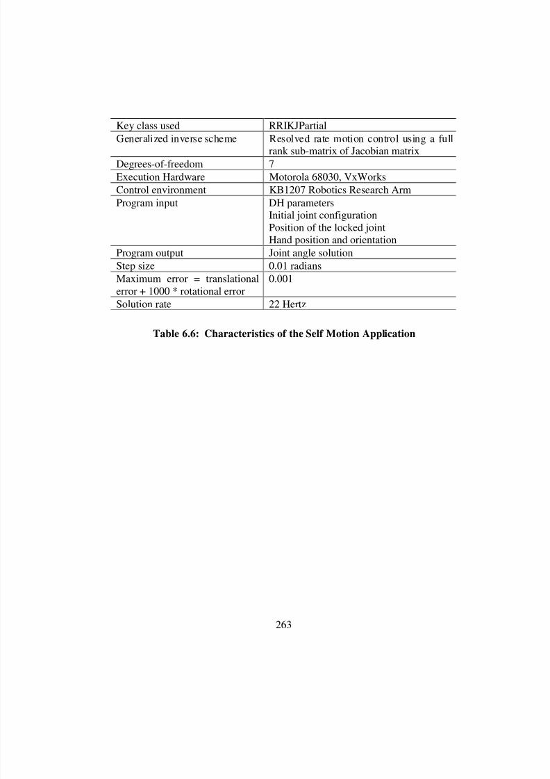
8/3/2019 Chetan Kapoor Dissertation
http://slidepdf.com/reader/full/chetan-kapoor-dissertation 287/612
263
Key class used RRIKJPartial
Generalized inverse scheme Resolved rate motion control using a fullrank sub-matrix of Jacobian matrix
Degrees-of-freedom 7
Execution Hardware Motorola 68030, VxWorks
Control environment KB1207 Robotics Research Arm
Program input DH parametersInitial joint configurationPosition of the locked jointHand position and orientation
Program output Joint angle solution
Step size 0.01 radians
Maximum error = translationalerror + 1000 * rotational error
0.001
Solution rate 22 Hertz
Table 6.6: Characteristics of the Self Motion Application

8/3/2019 Chetan Kapoor Dissertation
http://slidepdf.com/reader/full/chetan-kapoor-dissertation 288/612
264
6.2.4. Real-Time Generalized Ten Degrees-of-Freedom Inverse
This application program demonstrates the use of OSCAR architecture for
real-time interactive control of a ten DOF robot in Cartesian space. The robot
used for this purpose is a composite of the three DOF torso of the Robotics
Research dual arm and the left KB1207 arm of the dual-arm. The DH parameters
for this serial arm are listed in Table 6.7 (DH parameters by Rich Hooper). This
robot is interactively controlled by the TeachBall manual controller. The OSCAR
class RRIKJForGTSix is used for computing the inverse of this robot.
End-effector remains
Stationary
Self-Motion
Figure 6.3: Robotics Research KB1207 Going Through Self Motion.
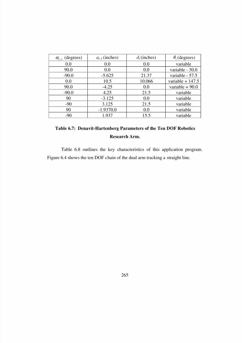
8/3/2019 Chetan Kapoor Dissertation
http://slidepdf.com/reader/full/chetan-kapoor-dissertation 289/612
265
Table 6.8 outlines the key characteristics of this application program.
Figure 6.4 shows the ten DOF chain of the dual arm tracking a straight line.
α i−1
(degrees) ai-1
(inches) d i(inches)
i(degrees)
0.0 0.0 0.0 variable
90.0 0.0 0.0 variable - 30.0
-90.0 -5.625 21.37 variable - 57.5
0.0 10.5 10.066 variable + 147.5
90.0 -4.25 0.0 variable + 90.0
-90.0 4.25 21.5 variable
90 -3.125 0.0 variable
-90 3.125 21.5 variable
90 -1.9370.0 0.0 variable
-90 1.937 15.5 variable
Table 6.7: Denavit-Hartenberg Parameters of the Ten DOF Robotics
Research Arm.

8/3/2019 Chetan Kapoor Dissertation
http://slidepdf.com/reader/full/chetan-kapoor-dissertation 290/612
266
Some of the goals of this research that were demonstrated by this program
are as follows:
Generality: The RRIKJForGTSix class that was used for the application
discussed in Section 6.2.2 is used for this application. This clearly depicts the
generalized nature of the inverse kinematics components that are a part of
OSCAR.
Real-time control: The inverse kinematics is computed online in real-time and
the output is channeled to a physical robot via a real-time control layer. This
clearly depicts the applicability of OSCAR to a real-time environment.
Manual Controller Integration: The TeachBall was used as the input device to
control the position and orientation of the end-effector of the robot. The
RRTeachBall component was used for interfacing to the TeachBall.
Key classes used RRIKJForGTSix, RRFKPosition
Generalized inverse scheme Resolved rate motion control using pseudoinverse
Degrees-of-freedom 10
Execution Hardware Motorola 68030, VxWorks
Control environment Robotics Research Dual Arm
Program input DH parametersInitial joint configurationHand position and orientation
Program output Joint angle solution
Step size 0.1 inches
Maximum error = translationalerror + 1000 * rotational error
0.001
Solution rate 30 Hertz
Table 6.8: Characteristics of the Ten DOF Real-Time Interactive Inverse
Application
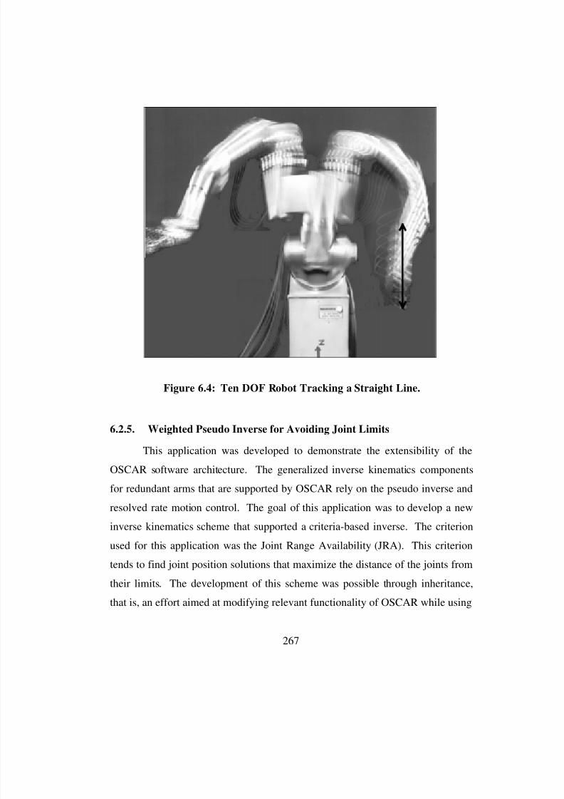
8/3/2019 Chetan Kapoor Dissertation
http://slidepdf.com/reader/full/chetan-kapoor-dissertation 291/612
267
Figure 6.4: Ten DOF Robot Tracking a Straight Line.
6.2.5. Weighted Pseudo Inverse for Avoiding Joint Limits
This application was developed to demonstrate the extensibility of the
OSCAR software architecture. The generalized inverse kinematics components
for redundant arms that are supported by OSCAR rely on the pseudo inverse and
resolved rate motion control. The goal of this application was to develop a new
inverse kinematics scheme that supported a criteria-based inverse. The criterion
used for this application was the Joint Range Availability (JRA). This criterion
tends to find joint position solutions that maximize the distance of the joints from
their limits. The development of this scheme was possible through inheritance,
that is, an effort aimed at modifying relevant functionality of OSCAR while using
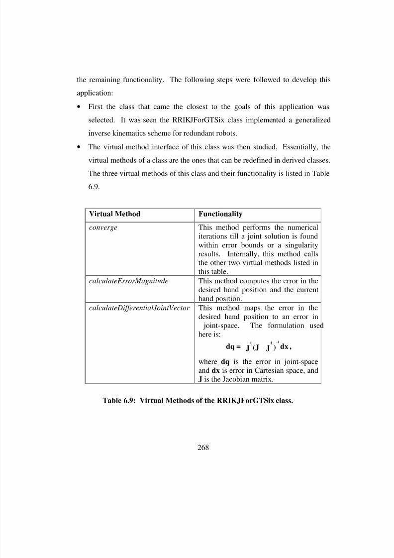
8/3/2019 Chetan Kapoor Dissertation
http://slidepdf.com/reader/full/chetan-kapoor-dissertation 292/612
268
the remaining functionality. The following steps were followed to develop this
application:
• First the class that came the closest to the goals of this application was
selected. It was seen the RRIKJForGTSix class implemented a generalized
inverse kinematics scheme for redundant robots.
• The virtual method interface of this class was then studied. Essentially, the
virtual methods of a class are the ones that can be redefined in derived classes.
The three virtual methods of this class and their functionality is listed in Table
6.9.
Virtual Method Functionality
converge This method performs the numericaliterations till a joint solution is foundwithin error bounds or a singularityresults. Internally, this method callsthe other two virtual methods listed inthis table.
calculateErrorMagnitude This method computes the error in the
desired hand position and the currenthand position.
calculateDifferentialJointVector This method maps the error in thedesired hand position to an error in joint-space. The formulation usedhere is:
dq = J (J J ) dxt t 1−
,
where dq is the error in joint-spaceand dx is error in Cartesian space, andJ is the Jacobian matrix.
Table 6.9: Virtual Methods of the RRIKJForGTSix class.
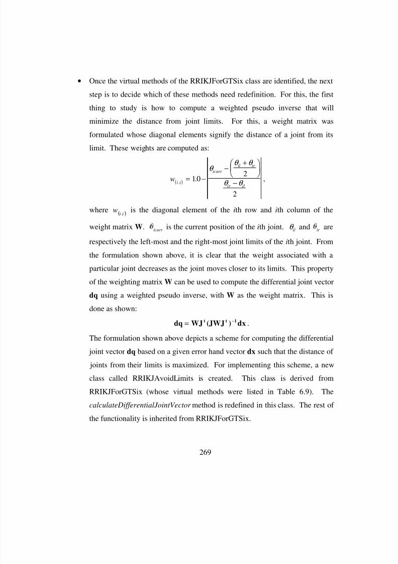
8/3/2019 Chetan Kapoor Dissertation
http://slidepdf.com/reader/full/chetan-kapoor-dissertation 293/612
269
• Once the virtual methods of the RRIKJForGTSix class are identified, the next
step is to decide which of these methods need redefinition. For this, the first
thing to study is how to compute a weighted pseudo inverse that will
minimize the distance from joint limits. For this, a weight matrix was
formulated whose diagonal elements signify the distance of a joint from its
limit. These weights are computed as:
( )wi i
icurr
il ir
ir il,
.= −−
+
−102
2
θ θ θ
θ θ ,
where( )
wi i,
is the diagonal element of the ith row and ith column of the
weight matrix W. icurr is the current position of the ith joint. θ il and ir are
respectively the left-most and the right-most joint limits of the ith joint. From
the formulation shown above, it is clear that the weight associated with a
particular joint decreases as the joint moves closer to its limits. This property
of the weighting matrix W can be used to compute the differential joint vector
dq using a weighted pseudo inverse, with W as the weight matrix. This isdone as shown:
dq WJ (JWJ ) dxt t 1= − .
The formulation shown above depicts a scheme for computing the differential
joint vector dq based on a given error hand vector dx such that the distance of
joints from their limits is maximized. For implementing this scheme, a new
class called RRIKJAvoidLimits is created. This class is derived from
RRIKJForGTSix (whose virtual methods were listed in Table 6.9). ThecalculateDifferentialJointVector method is redefined in this class. The rest of
the functionality is inherited from RRIKJForGTSix.
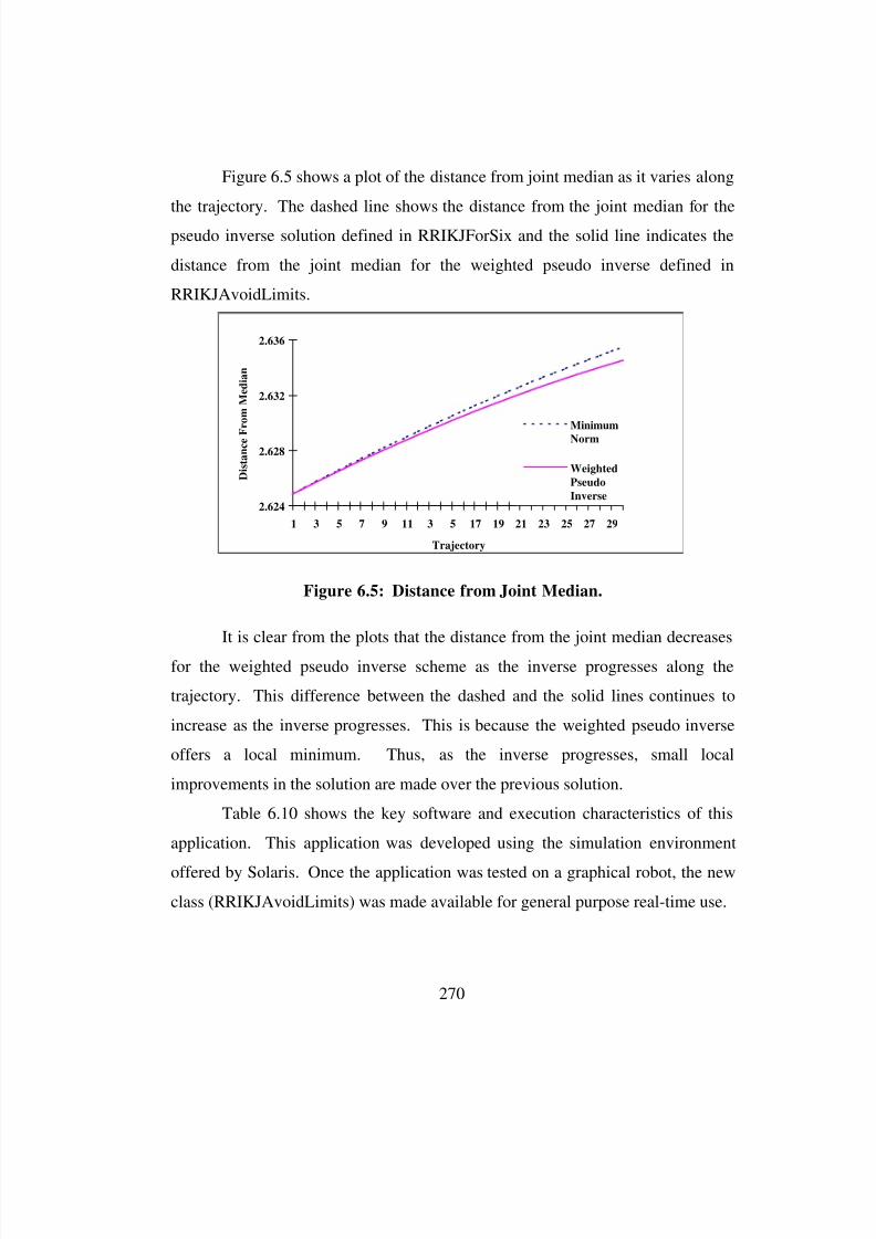
8/3/2019 Chetan Kapoor Dissertation
http://slidepdf.com/reader/full/chetan-kapoor-dissertation 294/612
270
Figure 6.5 shows a plot of the distance from joint median as it varies along
the trajectory. The dashed line shows the distance from the joint median for the
pseudo inverse solution defined in RRIKJForSix and the solid line indicates the
distance from the joint median for the weighted pseudo inverse defined in
RRIKJAvoidLimits.
2.624
2.628
2.632
2.636
1 3 5 7 9 11 3 5 17 19 21 23 25 27 29
Trajectory
D i s t a n c e F
r o m M e d i a n
Minimum
Norm
Weighted
Pseudo
Inverse
Figure 6.5: Distance from Joint Median.
It is clear from the plots that the distance from the joint median decreases
for the weighted pseudo inverse scheme as the inverse progresses along the
trajectory. This difference between the dashed and the solid lines continues to
increase as the inverse progresses. This is because the weighted pseudo inverse
offers a local minimum. Thus, as the inverse progresses, small local
improvements in the solution are made over the previous solution.
Table 6.10 shows the key software and execution characteristics of this
application. This application was developed using the simulation environment
offered by Solaris. Once the application was tested on a graphical robot, the new
class (RRIKJAvoidLimits) was made available for general purpose real-time use.

8/3/2019 Chetan Kapoor Dissertation
http://slidepdf.com/reader/full/chetan-kapoor-dissertation 295/612
271
The key goal that was demonstrated by this application is:
Extensibility: The key purpose of this application was to demonstrate the
extensibility that is built into the OSCAR architecture. It was seen in thisapplication that the developer could replace relevant parts of existing software
classes with other desired functionality. The remaining functionality of the
software class is reused in the new class that is designed by the developer. This
ability of the software supports rapid-prototyping.
6.2.6. Criteria-based Generalized Inverse
The main purpose of this application was to develop a criteria-based
generalized inverse kinematics scheme using the existing software components
provided by OSCAR. The scheme to be implemented uses the hybrid formulation
that is described in Chapter Three. This scheme basically has two steps. The first
step is the generation of a set of joint-space options that satisfy a desired end-
Key classes used RRIKJForGTSix, RRFKPosition
New class(es) developed RRIKJAvoidLimits
Generalized inverse scheme Resolved rate motion control usingweighted pseudo inverse
Degrees-of-freedom 7
Execution Hardware SUN SPARC 20-61 (Solaris)
Control environment Robotics Research Dual Arm
Program input DH parametersInitial joint configurationHand position and orientation
Program output Joint angle solution
Step size 0.1 inchesMaximum error = translationalerror + 1000 * rotational error
0.001
Solution rate 720 Hertz
Table 6.10: Characteristics of the Weighted Pseudo Inverse Application.
8/3/2019 Chetan Kapoor Dissertation
http://slidepdf.com/reader/full/chetan-kapoor-dissertation 296/612
272
effector constraint. The next step is the ranking of these options based on a set of
performance criteria. This algorithm was implemented using the RRIKJPartial
class, the RRPerformancCriteria classes, and the RRPCFusion class. The
RRIKJPartial class was used to generate a set of joint-space options. The
RRPerformanceCriteria classes were used to create three independent criteria for
this application. These three criteria were then supplied to the RRPCFusion class
for criteria fusion. The RRPCFusion was then supplied the joint-space options
that were generated by the RRIKJPartial class. These options were then ranked
by the RRPCFusion class.
This particular application was developed for a seven DOF robot arm. A
real-time implementation of this scheme was tested on the left arm of the
Robotics Research Dual-Arm robot. For comparison purposes this application
supported both the criteria-based inverse and the resolved rate motion control
scheme using the pseudo-inverse. The right arm of the dual-arm was used for the
pseudo inverse. The user of this application could interactively control both the
arms in end-effector space using the TeachBall manual controller. Additionally,
this application also demonstrated the simultaneous use of a simulation and real-time environment. This means that when the physical robot was commanded, the
graphical simulation of the dual-arm also imitated the movement of the physical
robot. The key operational characteristics of this application are listed in Table
6.11. For greater details about these application see Section 3.5.
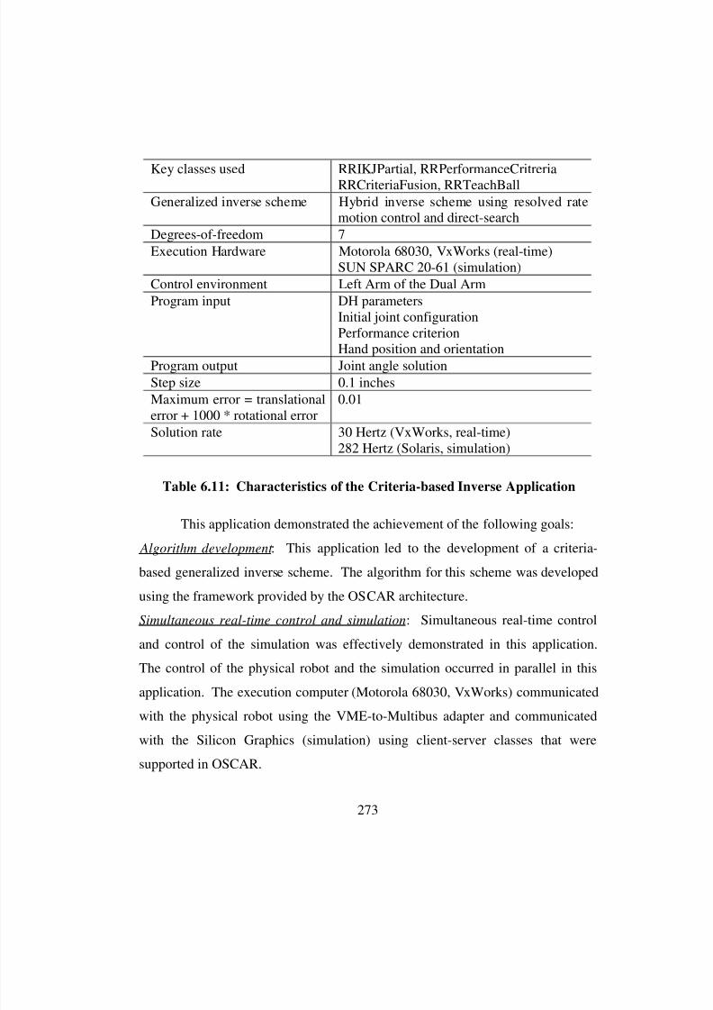
8/3/2019 Chetan Kapoor Dissertation
http://slidepdf.com/reader/full/chetan-kapoor-dissertation 297/612
273
This application demonstrated the achievement of the following goals: Algorithm development : This application led to the development of a criteria-
based generalized inverse scheme. The algorithm for this scheme was developed
using the framework provided by the OSCAR architecture.
Simultaneous real-time control and simulation: Simultaneous real-time control
and control of the simulation was effectively demonstrated in this application.
The control of the physical robot and the simulation occurred in parallel in this
application. The execution computer (Motorola 68030, VxWorks) communicated
with the physical robot using the VME-to-Multibus adapter and communicated
with the Silicon Graphics (simulation) using client-server classes that were
supported in OSCAR.
Key classes used RRIKJPartial, RRPerformanceCritreriaRRCriteriaFusion, RRTeachBall
Generalized inverse scheme Hybrid inverse scheme using resolved ratemotion control and direct-search
Degrees-of-freedom 7
Execution Hardware Motorola 68030, VxWorks (real-time)SUN SPARC 20-61 (simulation)
Control environment Left Arm of the Dual Arm
Program input DH parametersInitial joint configurationPerformance criterion
Hand position and orientationProgram output Joint angle solution
Step size 0.1 inches
Maximum error = translationalerror + 1000 * rotational error
0.01
Solution rate 30 Hertz (VxWorks, real-time)282 Hertz (Solaris, simulation)
Table 6.11: Characteristics of the Criteria-based Inverse Application
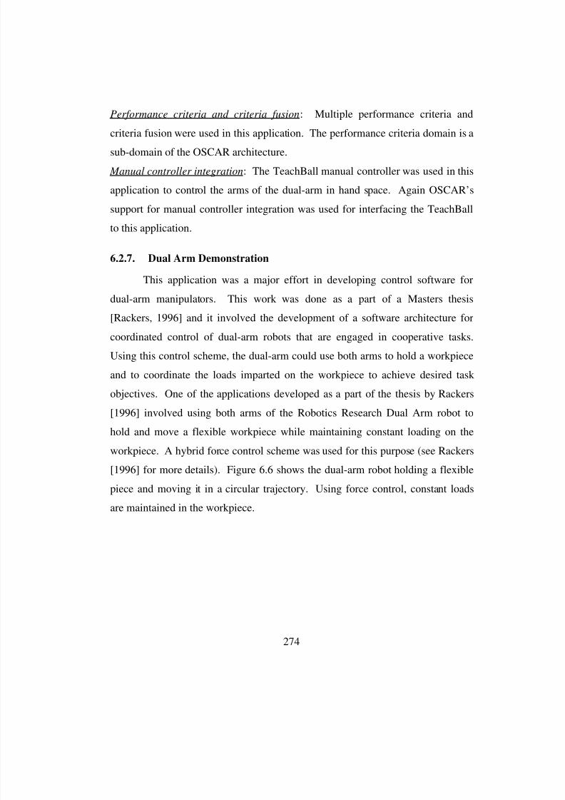
8/3/2019 Chetan Kapoor Dissertation
http://slidepdf.com/reader/full/chetan-kapoor-dissertation 298/612
274
Performance criteria and criteria fusion: Multiple performance criteria and
criteria fusion were used in this application. The performance criteria domain is a
sub-domain of the OSCAR architecture.
Manual controller integration: The TeachBall manual controller was used in this
application to control the arms of the dual-arm in hand space. Again OSCAR’s
support for manual controller integration was used for interfacing the TeachBall
to this application.
6.2.7. Dual Arm Demonstration
This application was a major effort in developing control software for
dual-arm manipulators. This work was done as a part of a Masters thesis
[Rackers, 1996] and it involved the development of a software architecture for
coordinated control of dual-arm robots that are engaged in cooperative tasks.
Using this control scheme, the dual-arm could use both arms to hold a workpiece
and to coordinate the loads imparted on the workpiece to achieve desired task
objectives. One of the applications developed as a part of the thesis by Rackers
[1996] involved using both arms of the Robotics Research Dual Arm robot to
hold and move a flexible workpiece while maintaining constant loading on the
workpiece. A hybrid force control scheme was used for this purpose (see Rackers
[1996] for more details). Figure 6.6 shows the dual-arm robot holding a flexible
piece and moving it in a circular trajectory. Using force control, constant loads
are maintained in the workpiece.
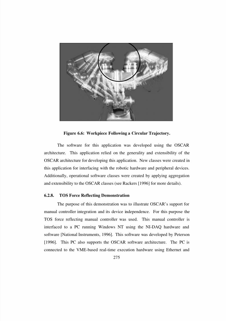
8/3/2019 Chetan Kapoor Dissertation
http://slidepdf.com/reader/full/chetan-kapoor-dissertation 299/612
275
Figure 6.6: Workpiece Following a Circular Trajectory.
The software for this application was developed using the OSCAR
architecture. This application relied on the generality and extensibility of the
OSCAR architecture for developing this application. New classes were created in
this application for interfacing with the robotic hardware and peripheral devices.Additionally, operational software classes were created by applying aggregation
and extensibility to the OSCAR classes (see Rackers [1996] for more details).
6.2.8. TOS Force Reflecting Demonstration
The purpose of this demonstration was to illustrate OSCAR’s support for
manual controller integration and its device independence. For this purpose the
TOS force reflecting manual controller was used. This manual controller is
interfaced to a PC running Windows NT using the NI-DAQ hardware and
software [National Instruments, 1996]. This software was developed by Peterson
[1996]. This PC also supports the OSCAR software architecture. The PC is
connected to the VME-based real-time execution hardware using Ethernet and
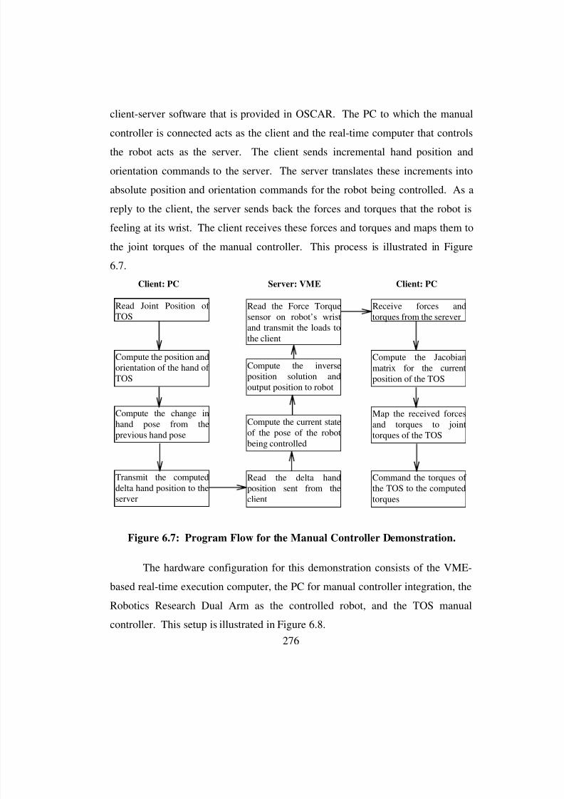
8/3/2019 Chetan Kapoor Dissertation
http://slidepdf.com/reader/full/chetan-kapoor-dissertation 300/612
276
client-server software that is provided in OSCAR. The PC to which the manual
controller is connected acts as the client and the real-time computer that controls
the robot acts as the server. The client sends incremental hand position and
orientation commands to the server. The server translates these increments into
absolute position and orientation commands for the robot being controlled. As a
reply to the client, the server sends back the forces and torques that the robot is
feeling at its wrist. The client receives these forces and torques and maps them to
the joint torques of the manual controller. This process is illustrated in Figure
6.7.
Read Joint Position of TOS
Compute the position andorientation of the hand of TOS
Compute the change inhand pose from theprevious hand pose
Transmit the computeddelta hand position to theserver
Read the Force Torquesensor on robot’s wristand transmit the loads tothe client
Compute the inverseposition solution andoutput position to robot
Compute the current stateof the pose of the robotbeing controlled
Read the delta handposition sent from theclient
Receive forces andtorques from the serever
Compute the Jacobianmatrix for the currentposition of the TOS
Map the received forcesand torques to jointtorques of the TOS
Command the torques of the TOS to the computedtorques
Client: PC Server: VME Client: PC
Figure 6.7: Program Flow for the Manual Controller Demonstration.
The hardware configuration for this demonstration consists of the VME-
based real-time execution computer, the PC for manual controller integration, the
Robotics Research Dual Arm as the controlled robot, and the TOS manual
controller. This setup is illustrated in Figure 6.8.
8/3/2019 Chetan Kapoor Dissertation
http://slidepdf.com/reader/full/chetan-kapoor-dissertation 301/612
277
The key operational characteristics of this application are listed in Table
6.12. The communication rate listed in Table 6.12 is the average data transfer
rate that was achieved between the Windows NT PC and the VME-based
execution environment.
Windows NT PC
(Client)
VME VxWorks
(Server)
Ethernet
Analog I/O
Bus-to-Bus Communication
TOS Manual
Controller
Robotics ResearchDual Arm Robot
Figure 6.8: Hardware Setup for Manual Controller Demonstration.
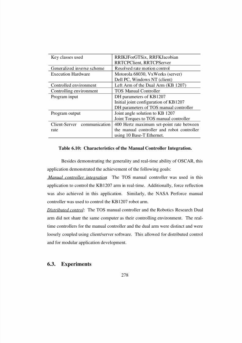
8/3/2019 Chetan Kapoor Dissertation
http://slidepdf.com/reader/full/chetan-kapoor-dissertation 302/612
278
Besides demonstrating the generality and real-time ability of OSCAR, this
application demonstrated the achievement of the following goals:
Manual controller integration: The TOS manual controller was used in this
application to control the KB1207 arm in real-time. Additionally, force reflection
was also achieved in this application. Similarly, the NASA Perforce manual
controller was used to control the KB1207 robot arm.
Distributed control: The TOS manual controller and the Robotics Research Dual
arm did not share the same computer as their controlling environment. The real-
time controllers for the manual controller and the dual arm were distinct and were
loosely coupled using client/server software. This allowed for distributed control
and for modular application development.
6.3. Experiments
Key classes used RRIKJForGTSix, RRFKJacobianRRTCPClient, RRTCPServer
Generalized inverse scheme Resolved rate motion control
Execution Hardware Motorola 68030, VxWorks (server)Dell PC, Windows NT (client)
Controlled environment Left Arm of the Dual Arm (KB 1207)
Controlling environment TOS Manual Controller
Program input DH parameters of KB1207Initial joint configuration of KB1207DH parameters of TOS manual controller
Program output Joint angle solution to KB 1207
Joint Torques to TOS manual controllerClient-Server communicationrate
400 Hertz maximum set-point rate betweenthe manual controller and robot controllerusing 10 Base-T Ethernet.
Table 6.10: Characteristics of the Manual Controller Integration.
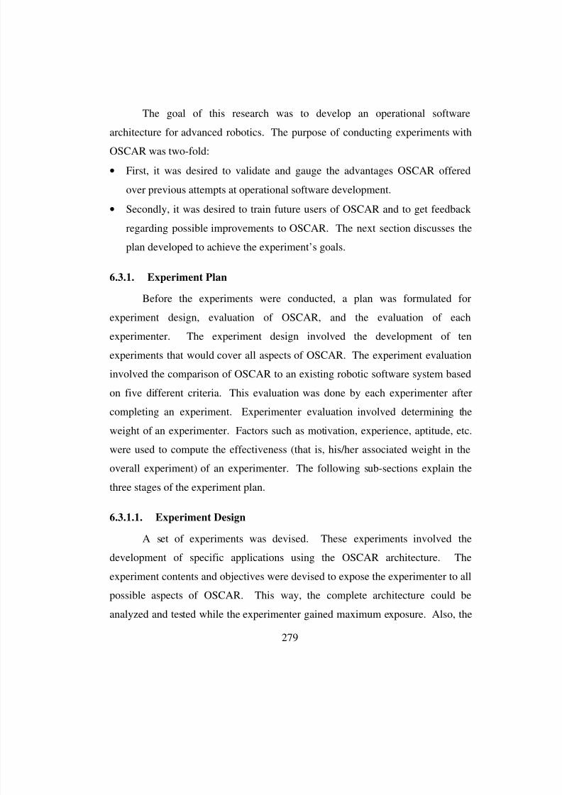
8/3/2019 Chetan Kapoor Dissertation
http://slidepdf.com/reader/full/chetan-kapoor-dissertation 303/612
279
The goal of this research was to develop an operational software
architecture for advanced robotics. The purpose of conducting experiments with
OSCAR was two-fold:
• First, it was desired to validate and gauge the advantages OSCAR offered
over previous attempts at operational software development.
• Secondly, it was desired to train future users of OSCAR and to get feedback
regarding possible improvements to OSCAR. The next section discusses the
plan developed to achieve the experiment’s goals.
6.3.1. Experiment Plan
Before the experiments were conducted, a plan was formulated for
experiment design, evaluation of OSCAR, and the evaluation of each
experimenter. The experiment design involved the development of ten
experiments that would cover all aspects of OSCAR. The experiment evaluation
involved the comparison of OSCAR to an existing robotic software system based
on five different criteria. This evaluation was done by each experimenter after
completing an experiment. Experimenter evaluation involved determining the
weight of an experimenter. Factors such as motivation, experience, aptitude, etc.
were used to compute the effectiveness (that is, his/her associated weight in the
overall experiment) of an experimenter. The following sub-sections explain the
three stages of the experiment plan.
6.3.1.1. Experiment Design
A set of experiments was devised. These experiments involved the
development of specific applications using the OSCAR architecture. The
experiment contents and objectives were devised to expose the experimenter to all
possible aspects of OSCAR. This way, the complete architecture could be
analyzed and tested while the experimenter gained maximum exposure. Also, the
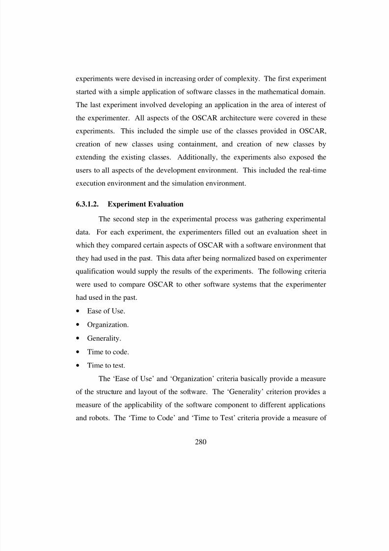
8/3/2019 Chetan Kapoor Dissertation
http://slidepdf.com/reader/full/chetan-kapoor-dissertation 304/612
280
experiments were devised in increasing order of complexity. The first experiment
started with a simple application of software classes in the mathematical domain.
The last experiment involved developing an application in the area of interest of
the experimenter. All aspects of the OSCAR architecture were covered in these
experiments. This included the simple use of the classes provided in OSCAR,
creation of new classes using containment, and creation of new classes by
extending the existing classes. Additionally, the experiments also exposed the
users to all aspects of the development environment. This included the real-time
execution environment and the simulation environment.
6.3.1.2. Experiment Evaluation
The second step in the experimental process was gathering experimental
data. For each experiment, the experimenters filled out an evaluation sheet in
which they compared certain aspects of OSCAR with a software environment that
they had used in the past. This data after being normalized based on experimenter
qualification would supply the results of the experiments. The following criteria
were used to compare OSCAR to other software systems that the experimenter
had used in the past.
• Ease of Use.
• Organization.
• Generality.
• Time to code.
• Time to test.
The ‘Ease of Use’ and ‘Organization’ criteria basically provide a measure
of the structure and layout of the software. The ‘Generality’ criterion provides a
measure of the applicability of the software component to different applications
and robots. The ‘Time to Code’ and ‘Time to Test’ criteria provide a measure of
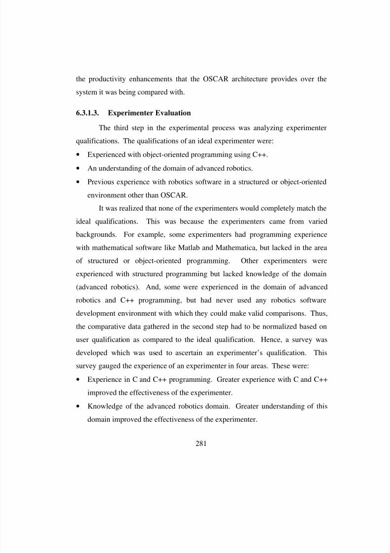
8/3/2019 Chetan Kapoor Dissertation
http://slidepdf.com/reader/full/chetan-kapoor-dissertation 305/612
281
the productivity enhancements that the OSCAR architecture provides over the
system it was being compared with.
6.3.1.3. Experimenter Evaluation
The third step in the experimental process was analyzing experimenter
qualifications. The qualifications of an ideal experimenter were:
• Experienced with object-oriented programming using C++.
• An understanding of the domain of advanced robotics.
• Previous experience with robotics software in a structured or object-oriented
environment other than OSCAR.
It was realized that none of the experimenters would completely match the
ideal qualifications. This was because the experimenters came from varied
backgrounds. For example, some experimenters had programming experience
with mathematical software like Matlab and Mathematica, but lacked in the area
of structured or object-oriented programming. Other experimenters were
experienced with structured programming but lacked knowledge of the domain
(advanced robotics). And, some were experienced in the domain of advancedrobotics and C++ programming, but had never used any robotics software
development environment with which they could make valid comparisons. Thus,
the comparative data gathered in the second step had to be normalized based on
user qualification as compared to the ideal qualification. Hence, a survey was
developed which was used to ascertain an experimenter’s qualification. This
survey gauged the experience of an experimenter in four areas. These were:
• Experience in C and C++ programming. Greater experience with C and C++
improved the effectiveness of the experimenter.
• Knowledge of the advanced robotics domain. Greater understanding of this
domain improved the effectiveness of the experimenter.
8/3/2019 Chetan Kapoor Dissertation
http://slidepdf.com/reader/full/chetan-kapoor-dissertation 306/612
282
• Experience with the software system the experimenter is comparing to
OSCAR. The experience with this software system should be at the same
level as the previous experience with programming in C/C++ type structured
or object-oriented environments. This is necessary for unbiased results. A
greater difference between an experimenter’s experience with C/C++ type
environments and the software system with which the comparison is being
made, lowers the effectiveness of the experimenter.
• How closely does the compared software system satisfy operational software
needs of advanced robotics (that is, the main purpose of OSCAR). This
criteria again decides the effectiveness of an experimenter. If the software
system with which the comparison is being made matches the operational
requirements that OSCAR fulfills, the greater the effectiveness of the
experimenter. For example, if the experimenter is comparing OSCAR to a
software based on a symbolic manipulation language like Mathematica, the
effectiveness of the experimenter would be considerably lower. However, the
effectiveness of an experimenter would be considerably higher if the
comparison is made with a library of C functions for robot control.
Besides the data collected from this survey, a measure of aptitude of the
experimenter and their motivation had to be generated. This was done by the
people who were monitoring the progress of the experiments and were
responsible for the academic supervision of the experimenters.
Finally, based on the degree of match between the experimenter
qualification and the ideal qualification, the aptitude, and motivation, different
weights would be generated for each experimenter. An experimenter with a
higher weight would have a greater impact on the results of the experiments. An
experimenter with a lower weight would have a lesser impact. After a weighting
measure has been generated for each experimenter, this weight would be applied
to the experimental data collected in step two. After this, the normalized
8/3/2019 Chetan Kapoor Dissertation
http://slidepdf.com/reader/full/chetan-kapoor-dissertation 307/612
283
experimental data is summed up for all experimenters. The results provide a
comparison between OSCAR and other robotic software environments.
The previous paragraphs discussed the plan that was to be followed for
successfully conducting experiments with OSCAR and generating some results.
To summarize, the key steps in the plan were:
• Devise a set of software experiments that were to be conducted by the
experimenters.
• Develop a set of criteria that would be used to make comparisons between
OSCAR and another software environment the experimenter is familiar with.
• Collect data regarding an experimenter’s experience, aptitude, and motivation.
Using this data, generate a weight for each experimenter.
• Normalize experimenter data based on their weight.
• Combine all normalized experimental data to come up with overall results.
6.3.2. Experimental Activity
The experimental activity began by the selection of a group of
experimenters. These experimenters were selected based on the followingfactors:
• The selected candidate’s academic research should be related to the OSCAR
software architecture.
• A selected candidate would in all probability be a future user of OSCAR.
• The selected candidate’s qualifications should closely match the qualifications
of the ideal experimenter.
Considering the factors mentioned above, eight candidates were selected. All
these candidates are members (students and staff) of the University of Texas,
Robotics Research Group. Six of these eight candidates (called candidates A
through F) were divided into three teams of two each. The teams were selected in
a manner such that one team member had a stronger programming background
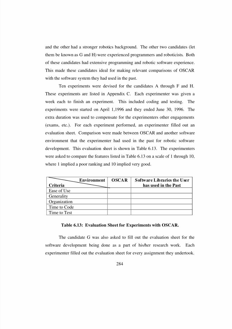
8/3/2019 Chetan Kapoor Dissertation
http://slidepdf.com/reader/full/chetan-kapoor-dissertation 308/612
284
and the other had a stronger robotics background. The other two candidates (let
them be known as G and H) were experienced programmers and roboticists. Both
of these candidates had extensive programming and robotic software experience.
This made these candidates ideal for making relevant comparisons of OSCAR
with the software system they had used in the past.
Ten experiments were devised for the candidates A through F and H.
These experiments are listed in Appendix C. Each experimenter was given a
week each to finish an experiment. This included coding and testing. The
experiments were started on April 1,1996 and they ended June 30, 1996. The
extra duration was used to compensate for the experimenters other engagements
(exams, etc.). For each experiment performed, an experimenter filled out an
evaluation sheet. Comparison were made between OSCAR and another software
environment that the experimenter had used in the past for robotic software
development. This evaluation sheet is shown in Table 6.13. The experimenters
were asked to compare the features listed in Table 6.13 on a scale of 1 through 10,
where 1 implied a poor ranking and 10 implied very good.
The candidate G was also asked to fill out the evaluation sheet for the
software development being done as a part of his/her research work. Each
experimenter filled out the evaluation sheet for every assignment they undertook.
Environment
Criteria
OSCAR Software Libraries the User
has used in the Past
Ease of Use
Generality
Organization
Time to Code
Time to Test
Table 6.13: Evaluation Sheet for Experiments with OSCAR.
8/3/2019 Chetan Kapoor Dissertation
http://slidepdf.com/reader/full/chetan-kapoor-dissertation 309/612
285
The results of each evaluation were then summed up and averaged for each
experimenter.
Besides filling out the evaluation sheet shown in Table 6.13, each
experimenter was asked to fill out a survey that was designed to gauge their
experience and qualifications. The data collected from this survey would be used
to weight each experimenter. The closer an experimenter came to the ideal
experimenter, the higher would be their weight. The survey filled out by the
experimenters is shown below:
• On a scale of 1 to 10, how would you gauge your experience with the
software system you are comparing OSCAR with, to programming in a
C/C++ type environment (use experience level before the beginning of the
experiments)?
C/C++ Type ___________ Compared Software System _______ _____
• What is the primary software system you were comparing OSCAR with (give
details)?
______________________________________________________________
______________________________________________________________
______________________________________________________________
______________________________________________________________
______________________________________________________________
The survey shown above tries to derive a measure of the experimenter’s
experience with C/C++ type programming environment as compared to the
software environment they are comparing OSCAR with. An experimenter who
has equivalent experience in both the environments is a better candidate than
someone who has dissimilar experience in the two environments. Additionally,
an experimenter is asked to describe the environment they are comparing OSCAR
with. Again, the weight carried by an experimenter is dependent on the
environment they are comparing OSCAR with. The assessment of how closely
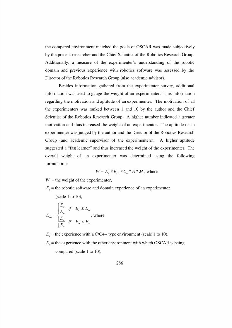
8/3/2019 Chetan Kapoor Dissertation
http://slidepdf.com/reader/full/chetan-kapoor-dissertation 310/612
286
the compared environment matched the goals of OSCAR was made subjectively
by the present researcher and the Chief Scientist of the Robotics Research Group.
Additionally, a measure of the experimenter’s understanding of the robotic
domain and previous experience with robotics software was assessed by the
Director of the Robotics Research Group (also academic advisor).
Besides information gathered from the experimenter survey, additional
information was used to gauge the weight of an experimenter. This information
regarding the motivation and aptitude of an experimenter. The motivation of all
the experimenters was ranked between 1 and 10 by the author and the Chief
Scientist of the Robotics Research Group. A higher number indicated a greater
motivation and thus increased the weight of an experimenter. The aptitude of an
experimenter was judged by the author and the Director of the Robotics Research
Group (and academic supervisor of the experimenters). A higher aptitude
suggested a “fast learner” and thus increased the weight of the experimenter. The
overall weight of an experimenter was determined using the following
formulation:
W E E C A M r co o= * * * * , where
W = the weight of the experimenter,
E r = the robotic software and domain experience of an experimenter
(scale 1 to 10),
E
E
E if E E
E
E if E E
co
c
o
c o
o
c
o c
=≤
<
, where
E c = the experience with a C/C++ type environment (scale 1 to 10),
E o = the experience with the other environment with which OSCAR is being
compared (scale 1 to 10),
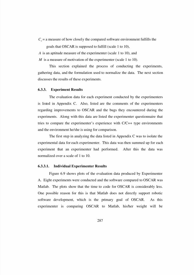
8/3/2019 Chetan Kapoor Dissertation
http://slidepdf.com/reader/full/chetan-kapoor-dissertation 311/612
287
C o = a measure of how closely the compared software environment fulfills the
goals that OSCAR is supposed to fulfill (scale 1 to 10), A is an aptitude measure of the experimenter (scale 1 to 10), and
M is a measure of motivation of the experimenter (scale 1 to 10).
This section explained the process of conducting the experiments,
gathering data, and the formulation used to normalize the data. The next section
discusses the results of these experiments.
6.3.3. Experiment Results
The evaluation data for each experiment conducted by the experimenters
is listed in Appendix C. Also, listed are the comments of the experimenters
regarding improvements to OSCAR and the bugs they encountered during the
experiments. Along with this data are listed the experimenter questionnaire that
tries to compare the experimenter’s experience with C/C++ type environments
and the environment he/she is using for comparison.
The first step in analyzing the data listed in Appendix C was to isolate the
experimental data for each experimenter. This data was then summed up for eachexperiment that an experimenter had performed. After this the data was
normalized over a scale of 1 to 10.
6.3.3.1. Individual Experimenter Results
Figure 6.9 shows plots of the evaluation data produced by Experimenter
A. Eight experiments were conducted and the software compared to OSCAR was
Matlab. The plots show that the time to code for OSCAR is considerably less.
One possible reason for this is that Matlab does not directly support robotic
software development, which is the primary goal of OSCAR. As this
experimenter is comparing OSCAR to Matlab, his/her weight will be

8/3/2019 Chetan Kapoor Dissertation
http://slidepdf.com/reader/full/chetan-kapoor-dissertation 312/612
288
considerably lowered (see Table 6.14). This is because Matlab does not satisfy
operational requirements for robotic software.
Figure 6.10 shows the plots of the evaluation data produced by
Experimenter B. Nine experiments were conducted by this experimenter. Of
these, the last experiment was self-defined in the area of interest of the
experimenter. The OSCAR environment was compared to the symbolic
manipulation software Mathematica. From the plots it is seen that the time to
code for OSCAR is considerably less. One reason given by the experimenter for
this was the inefficient programming environment offered by Mathematica. Also,
Mathematica does not directly support robotic software development.
Ease of Use Generality Organization 1/Code Time 1/TestTime
0.00
1.00
2.00
3.00
4.00
5.00
6.00
7.00
8.00
9.00
10.00
Ease of Use Generality Organization 1/Code Time 1/TestTime
OSCAR
Matlab
Figure 6.9: Averaged Evaluation Data for Experimenter A.
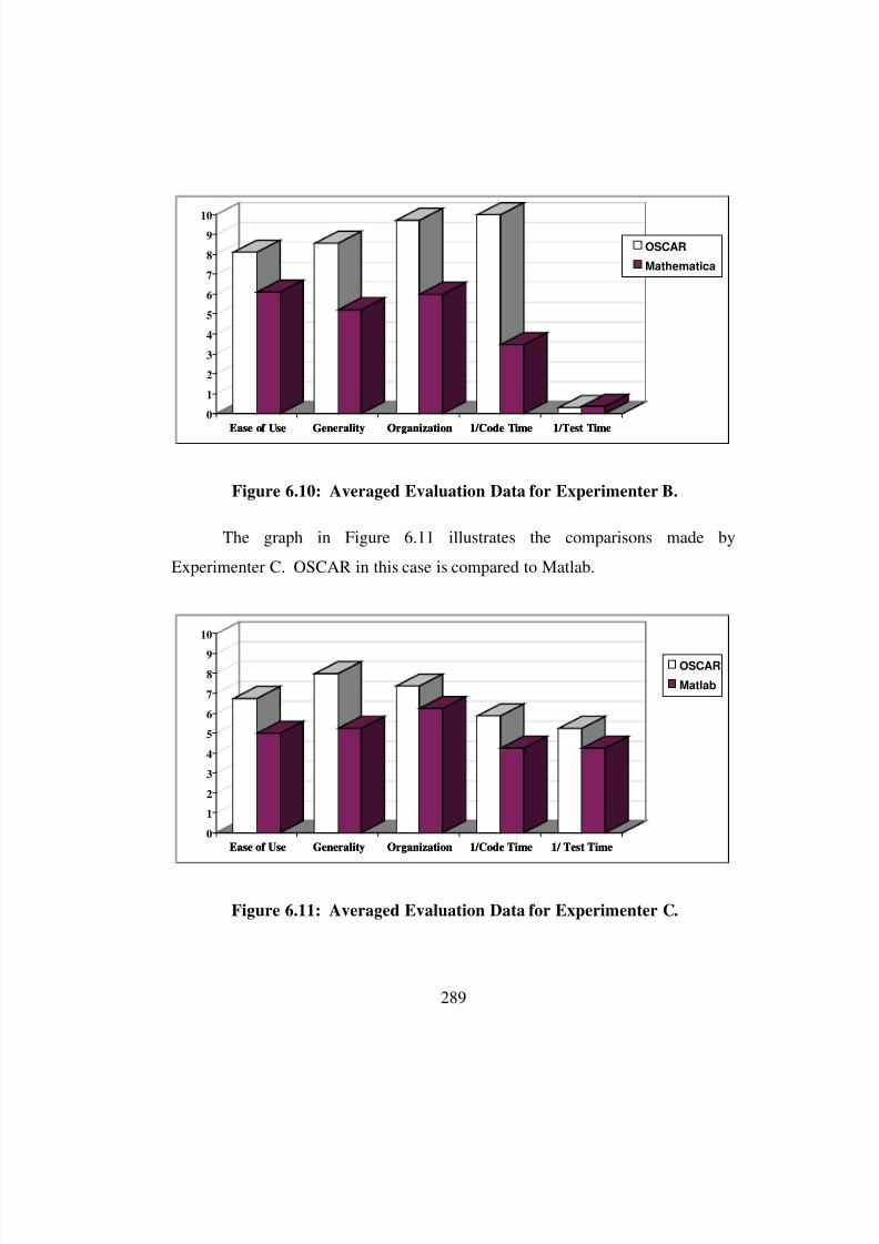
8/3/2019 Chetan Kapoor Dissertation
http://slidepdf.com/reader/full/chetan-kapoor-dissertation 313/612
289
The graph in Figure 6.11 illustrates the comparisons made by
Experimenter C. OSCAR in this case is compared to Matlab.
Ease of Use Generality Organization 1/Code Time 1/Test Time
0
1
2
3
4
5
6
7
8
9
10
Ease of Use Generality Organization 1/Code Time 1/Test Time
OSCAR
Mathematica
Figure 6.10: Averaged Evaluation Data for Experimenter B.
Ease of Use Generality Organization 1/Code Time 1/ Test Time
0
1
2
3
4
5
6
7
8
9
10
Ease of Use Generality Organization 1/Code Time 1/ Test Time
OSCAR
Matlab
Figure 6.11: Averaged Evaluation Data for Experimenter C.
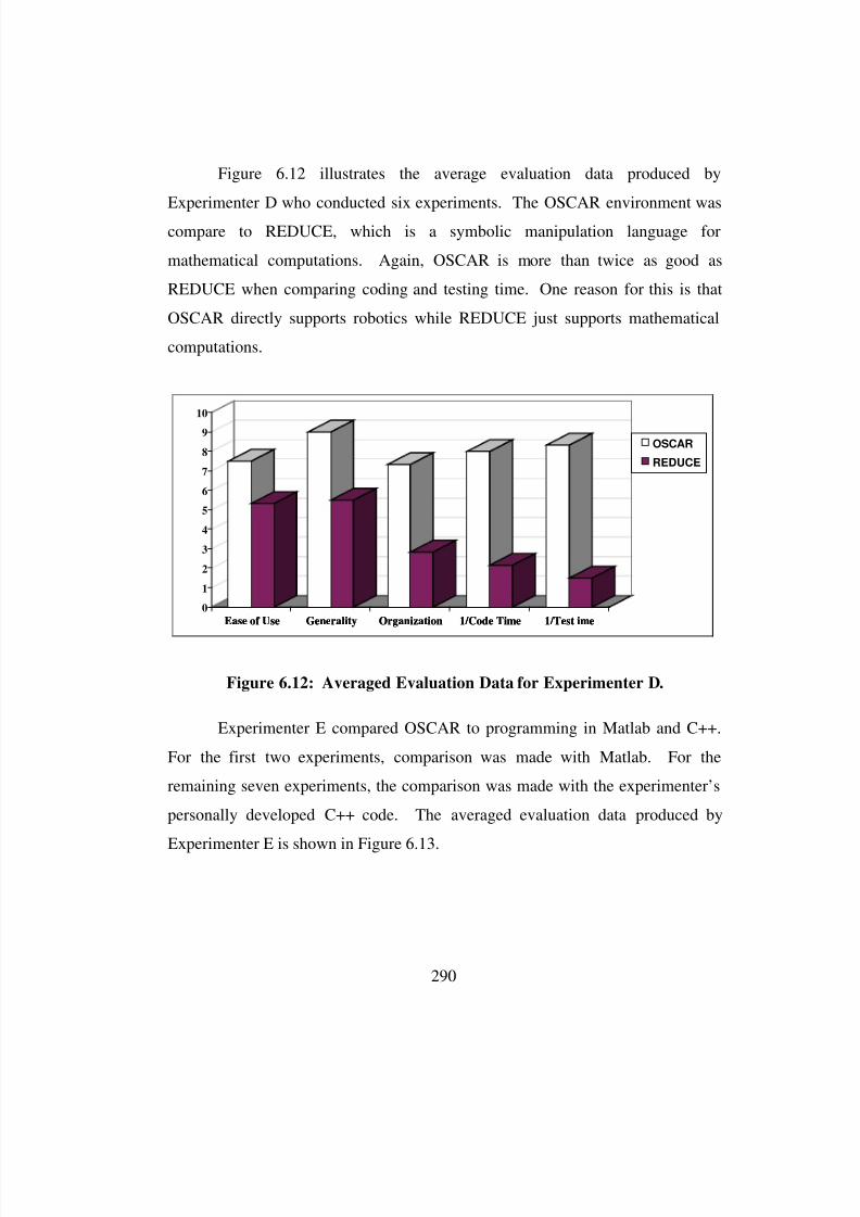
8/3/2019 Chetan Kapoor Dissertation
http://slidepdf.com/reader/full/chetan-kapoor-dissertation 314/612
290
Figure 6.12 illustrates the average evaluation data produced by
Experimenter D who conducted six experiments. The OSCAR environment was
compare to REDUCE, which is a symbolic manipulation language for
mathematical computations. Again, OSCAR is more than twice as good as
REDUCE when comparing coding and testing time. One reason for this is that
OSCAR directly supports robotics while REDUCE just supports mathematical
computations.
Experimenter E compared OSCAR to programming in Matlab and C++.
For the first two experiments, comparison was made with Matlab. For the
remaining seven experiments, the comparison was made with the experimenter’s
personally developed C++ code. The averaged evaluation data produced by
Experimenter E is shown in Figure 6.13.
Ease of Use Generality Organization 1/Code Time 1/Test ime
0
1
2
3
4
5
6
7
8
9
10
Ease of Use Generality Organization 1/Code Time 1/Test ime
OSCAR
REDUCE
Figure 6.12: Averaged Evaluation Data for Experimenter D.

8/3/2019 Chetan Kapoor Dissertation
http://slidepdf.com/reader/full/chetan-kapoor-dissertation 315/612
291
Experimenter F conducted eight experiments and compared OSCAR to
the Matlab programming environment. The evaluation data produced by this
experimenter is shown in Figure 6.14.
Ease of Use Generality Organization 1/Code Time 1/Test Time
0
1
2
3
4
5
6
7
8
9
10
Ease of Use Generality Organization 1/Code Time 1/Test Time
OSCAR
Matlab and C++ Code
Figure 6.13: Averaged Evaluation Data for Experimenter E.
Ease of Use Generality Organization 1/Code Time 1/Test Time
0
1
2
3
4
5
6
7
8
9
10
Ease of Use Generality Organization 1/Code Time 1/Test Time
OSCAR
Matlab
Figure 6.14: Averaged Evaluation Data for Experimenter F.
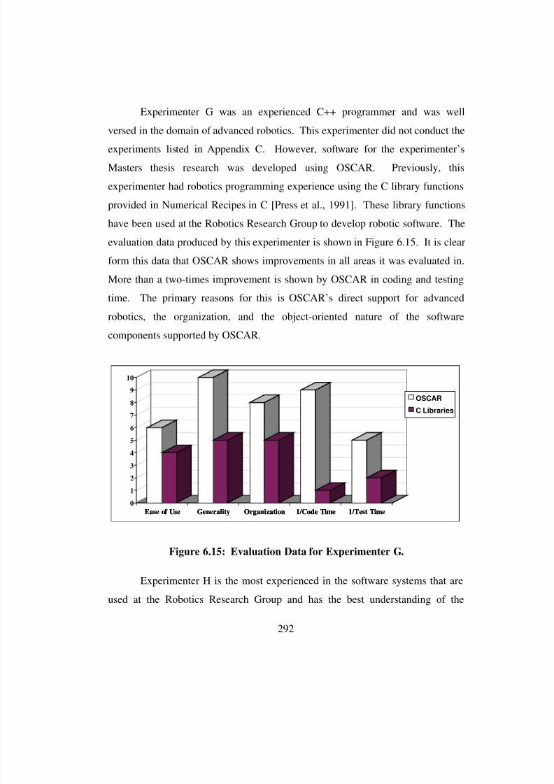
8/3/2019 Chetan Kapoor Dissertation
http://slidepdf.com/reader/full/chetan-kapoor-dissertation 316/612
292
Experimenter G was an experienced C++ programmer and was well
versed in the domain of advanced robotics. This experimenter did not conduct the
experiments listed in Appendix C. However, software for the experimenter’s
Masters thesis research was developed using OSCAR. Previously, this
experimenter had robotics programming experience using the C library functions
provided in Numerical Recipes in C [Press et al., 1991]. These library functions
have been used at the Robotics Research Group to develop robotic software. The
evaluation data produced by this experimenter is shown in Figure 6.15. It is clear
form this data that OSCAR shows improvements in all areas it was evaluated in.
More than a two-times improvement is shown by OSCAR in coding and testing
time. The primary reasons for this is OSCAR’s direct support for advanced
robotics, the organization, and the object-oriented nature of the software
components supported by OSCAR.
Experimenter H is the most experienced in the software systems that are
used at the Robotics Research Group and has the best understanding of the
Ease of Use Generality Organization 1/Code Time 1/Test Time
0
1
2
3
4
5
6
7
8
9
10
Ease of Use Generality Organization 1/Code Time 1/Test Time
OSCAR
C Libraries
Figure 6.15: Evaluation Data for Experimenter G.
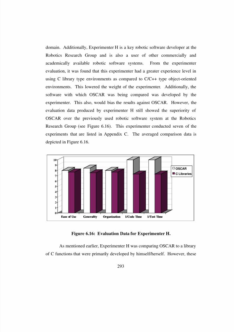
8/3/2019 Chetan Kapoor Dissertation
http://slidepdf.com/reader/full/chetan-kapoor-dissertation 317/612
293
domain. Additionally, Experimenter H is a key robotic software developer at the
Robotics Research Group and is also a user of other commercially and
academically available robotic software systems. From the experimenter
evaluation, it was found that this experimenter had a greater experience level in
using C library type environments as compared to C/C++ type object-oriented
environments. This lowered the weight of the experimenter. Additionally, the
software with which OSCAR was being compared was developed by the
experimenter. This also, would bias the results against OSCAR. However, the
evaluation data produced by experimenter H still showed the superiority of
OSCAR over the previously used robotic software system at the Robotics
Research Group (see Figure 6.16). This experimenter conducted seven of the
experiments that are listed in Appendix C. The averaged comparison data is
depicted in Figure 6.16.
As mentioned earlier, Experimenter H was comparing OSCAR to a library
of C functions that were primarily developed by himself/herself. However, these
Ease of Use Generality Organization 1/Code Time 1/Test Time
0
1
2
3
4
5
6
7
8
9
10
Ease of Use Generality Organization 1/Code Time 1/Test Time
OSCAR
C Libraries
Figure 6.16: Evaluation Data for Experimenter H.
8/3/2019 Chetan Kapoor Dissertation
http://slidepdf.com/reader/full/chetan-kapoor-dissertation 318/612
294
functions were not organized in a manner to promote their use by other
developers. This is evident from the quote by Experimenter H,
“It seems that using OSCAR is allowing some of our students with
limited software experience to write programs implementing very
complex geometry, mathematics, and kinematics. I don’t think they
would be able to write these programs from scratch without one or more
years of work. The comparison to the C environment we were using
previously is somewhat difficult. We are now experiencing much better
software reuse than we were before. Basically, over the previous 8 years
we had little to no software reuse. Now we are reusing software, but we
are making an effort to reuse the software. Before we had very little
reuse effort and very little reuse. Ultimately time will tell the success of
the reuse effort.”
Drawing inferences from Experimenter H’s comments, it is clear that
OSCAR is the first software environment that is being used by developers at the
Robotics Research Group. Also, significantly more effort would be necessary to
develop robotic programs without OSCAR. However, from Experimenter H’scomparison data (see Figure 6.16) it is clear that OSCAR does not show
significant improvement over robotic software that was previously used at the
Robotics Research Group. This result is understandable because the software
with which OSCAR is being compared was developed by Experimenter H. This
biases the results against OSCAR. Additionally, Experimenter H’s experience
with object-oriented systems is limited as compared to experience with structured
systems. Due to the lack of experience with object-oriented system, the reuse
potential of OSCAR was not evident to experimenter H. Experimenter G on the
other hand was experienced with structured and object-oriented systems.
Experimenter G had attempted robotic software development using the structured
environment that was previously available at the Robotics Research Group.

8/3/2019 Chetan Kapoor Dissertation
http://slidepdf.com/reader/full/chetan-kapoor-dissertation 319/612
295
However, Experimenter G shifted to OSCAR when it was made available. For
these reasons, Experimenter G possibly was the most effective experimenter. The
effectiveness of each experimenter is discussed in the next section.
6.3.3.2. Overall Experiment Results
Once the evaluation and comparison data was gathered for all
experimenters, the next step was the normalization and averaging of this data to
reach an overall result. This process is explained in this section.
The evaluation data produced by the experimenters is graphically
illustrated in Figures 6.9 to 6.16. The final step in the evaluation of OSCAR is
the normalization and averaging of the data produced by the various
experimenters. Before normalization, individual weights of each experimenter
had to be assessed based on experimenter experience, motivation, aptitude, and
the environment they were comparing OSCAR with. Section 6.3.1 discussed the
process and the formulation used in assessing the weight of an experimenter. The
data gathered for this purpose is listed in Table 6.14. The last column
(highlighted) of this table gives the overall weight of the experimenter. The
greater the weight of an experimenter, the greater is the impact on the overall
results of the experiments.
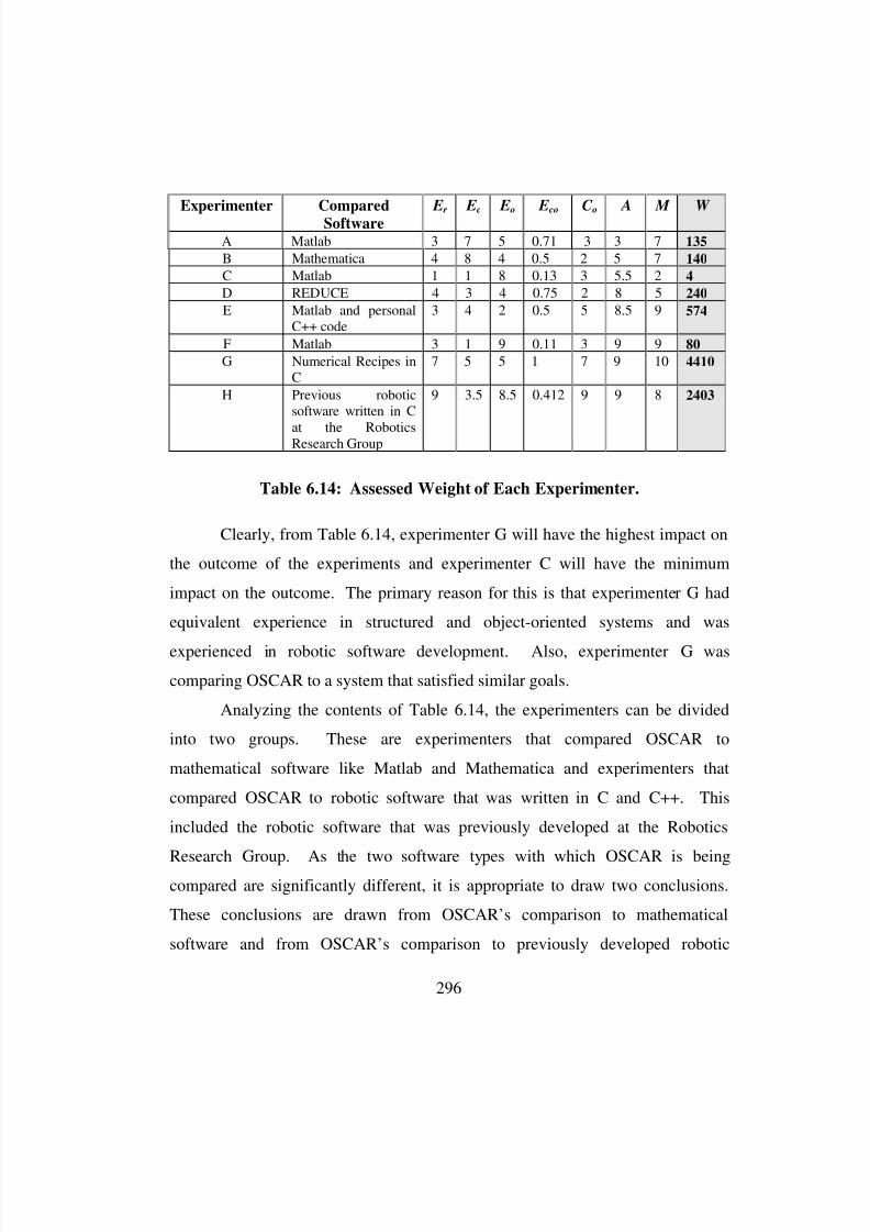
8/3/2019 Chetan Kapoor Dissertation
http://slidepdf.com/reader/full/chetan-kapoor-dissertation 320/612
296
Clearly, from Table 6.14, experimenter G will have the highest impact on
the outcome of the experiments and experimenter C will have the minimum
impact on the outcome. The primary reason for this is that experimenter G had
equivalent experience in structured and object-oriented systems and was
experienced in robotic software development. Also, experimenter G was
comparing OSCAR to a system that satisfied similar goals.
Analyzing the contents of Table 6.14, the experimenters can be divided
into two groups. These are experimenters that compared OSCAR to
mathematical software like Matlab and Mathematica and experimenters that
compared OSCAR to robotic software that was written in C and C++. This
included the robotic software that was previously developed at the Robotics
Research Group. As the two software types with which OSCAR is beingcompared are significantly different, it is appropriate to draw two conclusions.
These conclusions are drawn from OSCAR’s comparison to mathematical
software and from OSCAR’s comparison to previously developed robotic
Experimenter Compared
Software
E r E c E o E co C o A M W
A Matlab 3 7 5 0.71 3 3 7 135
B Mathematica 4 8 4 0.5 2 5 7 140
C Matlab 1 1 8 0.13 3 5.5 2 4
D REDUCE 4 3 4 0.75 2 8 5 240
E Matlab and personalC++ code
3 4 2 0.5 5 8.5 9 574
F Matlab 3 1 9 0.11 3 9 9 80
G Numerical Recipes inC
7 5 5 1 7 9 10 4410
H Previous roboticsoftware written in C
at the RoboticsResearch Group
9 3.5 8.5 0.412 9 9 8 2403
Table 6.14: Assessed Weight of Each Experimenter.

8/3/2019 Chetan Kapoor Dissertation
http://slidepdf.com/reader/full/chetan-kapoor-dissertation 321/612
297
software at the Robotics Research Group. These conclusions are discussed in the
following sections.
6.3.3.2.1. OSCAR Compared to Mathematical Software
From Table 6.14 it is clear that experimenters A, B, C, D, and F compared
OSCAR to mathematical software. These were Matlab, Mathematica, and
REDUCE. All these software products are used for mathematical modeling of
systems and do not satisfy operational requirements and are unsuitable for real-
time control. Considering the weight of each experimenter in this group, the
comparison data was averaged and the results are shown in Figure 6.17.
From Figure 6.17 it is clear that OSCAR fares better than mathematical
software in all aspects. The primary reason for this is the inability of
mathematical software to support large-scale program development and their lack
of direct support for robotic software. Additionally, these mathematical software
systems would not support a majority of applications that could use OSCAR (for
example, distributed real-time control).
Ease of Use Generality Organization 1/Code Time 1/Test Time
0
1
2
3
4
5
6
7
8
9
10
Ease of Use Generality Organization 1/Code Time 1/Test Time
OSCAR
MathematicalSoftware
Figure 6.17: OSCAR Compared to Mathematical Software.
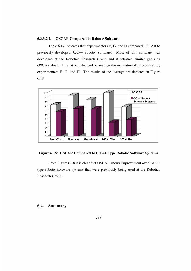
8/3/2019 Chetan Kapoor Dissertation
http://slidepdf.com/reader/full/chetan-kapoor-dissertation 322/612
298
6.3.3.2.2. OSCAR Compared to Robotic Software
Table 6.14 indicates that experimenters E, G, and H compared OSCAR topreviously developed C/C++ robotic software. Most of this software was
developed at the Robotics Research Group and it satisfied similar goals as
OSCAR does. Thus, it was decided to average the evaluation data produced by
experimenters E, G, and H. The results of the average are depicted in Figure
6.18.
From Figure 6.18 it is clear that OSCAR shows improvement over C/C++
type robotic software systems that were previously being used at the Robotics
Research Group.
6.4. Summary
Ease of Use Generality Organization 1/Code Time 1/Test Time
0
1
2
3
4
5
6
7
8
9
10
Ease of Use Generality Organization 1/Code Time 1/Test Time
OSCAR
C/C++ RoboticSoftware Systems
Figure 6.18: OSCAR Compared to C/C++ Type Robotic Software Systems.
8/3/2019 Chetan Kapoor Dissertation
http://slidepdf.com/reader/full/chetan-kapoor-dissertation 323/612
299
This chapter presented the validation for this research. The OSCAR
architecture was demonstrated through example applications. These applications
include the demonstration of OSCAR’s support for simulation and real-time
computing. The generalized kinematics and other domains built into OSCAR
were demonstrated. Operational characteristics of each application were also
discussed. Additionally, OSCAR’s support for manual controller integration and
distributed computing was demonstrated. The ability to develop new components
via aggregation and extension was also demonstrated.
A desired characteristic of this research was that OSCAR should reduce
robot control program development time by 50%. This hypothesis was tested by
conducting experiments with OSCAR. For this purpose eight experimenters were
chosen and a set of ten experiments designed. The experimenters completed
these experiments in four months and filled out an evaluation sheet. In this they
compared OSCAR to a software system which they had previously used for
robotic software development. Besides evaluation of OSCAR by experimenters,
an evaluation of experimenters was also performed by the author and staff at the
Robotics Research Group. Considering experimenter evaluation, weights wereassigned to each experimenter. An experimenter with a higher weight had a
greater impact on the final outcome of the experiments. The experimenters
compared OSCAR to primarily two software systems. One was mathematical
software (Matlab, Mathematica, etc.) and the other was robotic software written
in C/C++ that was previously used at the Robotics Research Group. The
averaged data for each group showed that OSCAR was more general, easy to use,
and better organized than mathematical software and C/C++ type robotic software
that was previously used at the Robotics Research Group. Also, OSCAR reduced
program development time (time to code and time to test) by a factor of three as
compared to mathematical software and C/C++ type robotic software that was
previously being used at the Robotics Research Group.

8/3/2019 Chetan Kapoor Dissertation
http://slidepdf.com/reader/full/chetan-kapoor-dissertation 324/612
300

8/3/2019 Chetan Kapoor Dissertation
http://slidepdf.com/reader/full/chetan-kapoor-dissertation 325/612
301
Chapter Seven
7. Summary and Proposed Future Development
A summary of the previous chapters of this report is provided in the first
section of this chapter with primary conclusions. In the second section,
applications of this research, recommendations and suggestions for future
directions of this development are discussed.
7.1. Summary and Conclusions
This section contains the summary of the report. The summary of the
objectives, the literature review, the research accomplished, and demonstrations is
provided.
The overall goal of this research has been to develop a software
architecture that supports control program development for advanced robotics.
This software architecture is called “Operational Software Components for
Advanced Robotics” (OSCAR) in this report. The research objectives for
accomplishing this goal were discussed in Chapter One and are summarized in
Table 7.1 (see Section 1.2). Chapter One also discussed the key characteristics of
an advanced robotic system. These were, modularity, generalized kinematics,
generalized dynamics, deflection modeling, fault-tolerance, and decision making
(see Sections 1.5 to 1.9). Additionally, the three layers of robotic software at the
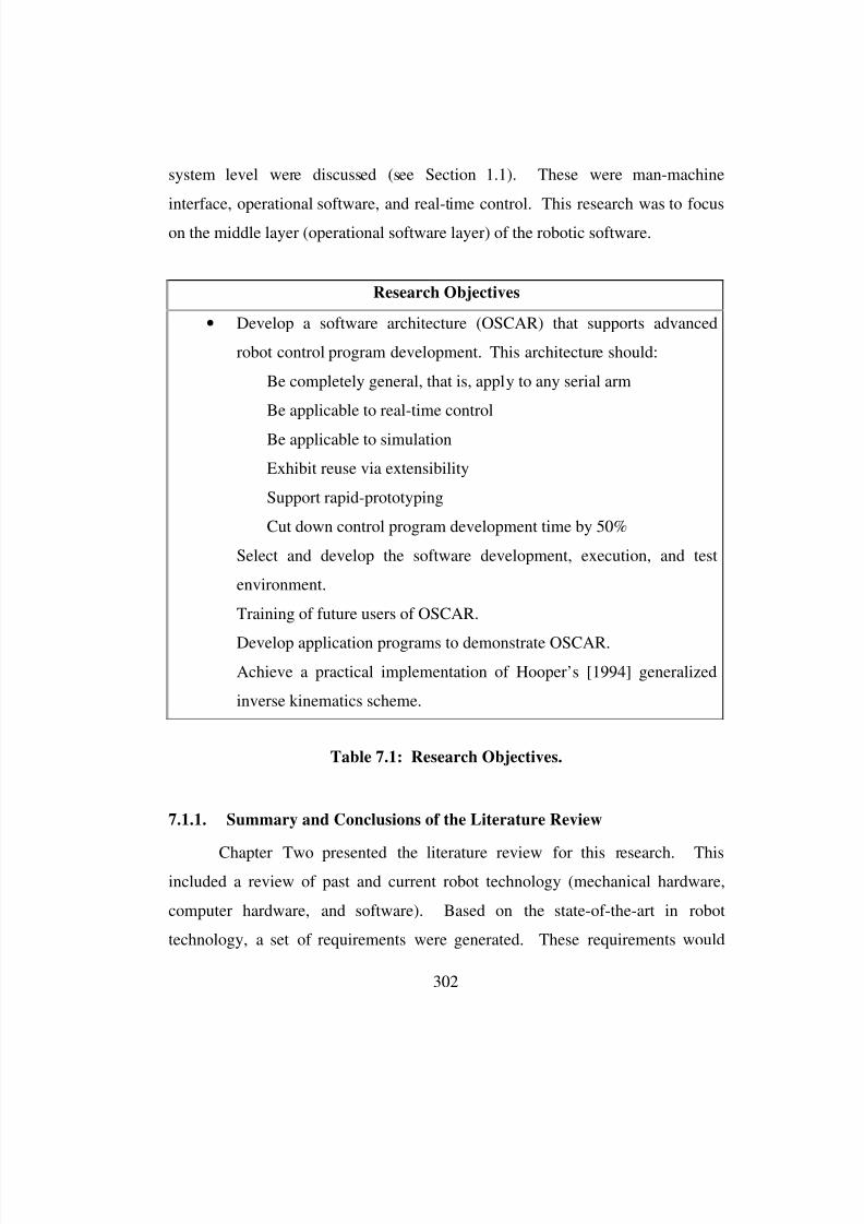
8/3/2019 Chetan Kapoor Dissertation
http://slidepdf.com/reader/full/chetan-kapoor-dissertation 326/612
302
system level were discussed (see Section 1.1). These were man-machine
interface, operational software, and real-time control. This research was to focus
on the middle layer (operational software layer) of the robotic software.
7.1.1. Summary and Conclusions of the Literature Review
Chapter Two presented the literature review for this research. Thisincluded a review of past and current robot technology (mechanical hardware,
computer hardware, and software). Based on the state-of-the-art in robot
technology, a set of requirements were generated. These requirements would
Research Objectives
• Develop a software architecture (OSCAR) that supports advanced
robot control program development. This architecture should:
Be completely general, that is, apply to any serial arm
Be applicable to real-time control
Be applicable to simulation
Exhibit reuse via extensibility
Support rapid-prototyping
Cut down control program development time by 50%
Select and develop the software development, execution, and test
environment.
Training of future users of OSCAR.
Develop application programs to demonstrate OSCAR.
Achieve a practical implementation of Hooper’s [1994] generalized
inverse kinematics scheme.
Table 7.1: Research Objectives.
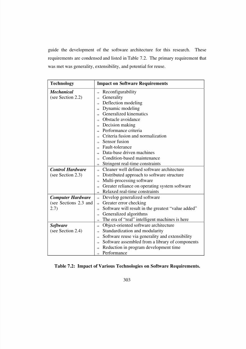
8/3/2019 Chetan Kapoor Dissertation
http://slidepdf.com/reader/full/chetan-kapoor-dissertation 327/612
303
guide the development of the software architecture for this research. These
requirements are condensed and listed in Table 7.2. The primary requirement that
was met was generality, extensibility, and potential for reuse.
Technology Impact on Software Requirements
Mechanical (see Section 2.2)
⇒ Reconfigurability⇒ Generality⇒ Deflection modeling⇒ Dynamic modeling⇒ Generalized kinematics⇒ Obstacle avoidance⇒ Decision making⇒ Performance criteria⇒ Criteria fusion and normalization⇒ Sensor fusion⇒ Fault-tolerance⇒ Data-base driven machines⇒ Condition-based maintenance⇒ Stringent real-time constraints
Control Hardware(see Section 2.3)
⇒ Cleaner well defined software architecture⇒ Distributed approach to software structure⇒ Multi-processing software⇒ Greater reliance on operating system software⇒ Relaxed real-time constraints
Computer Hardware(see Sections 2.3 and2.7)
⇒ Develop generalized software⇒ Greater error checking⇒ Software will result in the greatest “value added”⇒ Generalized algorithms⇒ The era of “real” intelligent machines is here
Software(see Section 2.4)
⇒ Object-oriented software architecture⇒ Standardization and modularity⇒ Software reuse via generality and extensibility⇒ Software assembled from a library of components⇒ Reduction in program development time⇒ Performance
Table 7.2: Impact of Various Technologies on Software Requirements.

8/3/2019 Chetan Kapoor Dissertation
http://slidepdf.com/reader/full/chetan-kapoor-dissertation 328/612
304
Once the software requirements for an advanced robot were generated,
existing robotic software environments were reviewed (see Section 2.6). A brief
analysis of these environments is listed in Table 7.3. The primary environment
for this software development was taken to be object-oriented structures.

8/3/2019 Chetan Kapoor Dissertation
http://slidepdf.com/reader/full/chetan-kapoor-dissertation 329/612
305
Research Summary
RCCL(see Section 2.6.2.1)
− Based on the C programming language− Uses UNIX for real-time control− Advanced robotics not supported− Based on structured design− Software generality and extensibility missing
RIPE(see Section 2.6.2.2)
− Primarily a robot programming environment− Uses object-oriented design to provide standard robot
programming interface− Advanced robotics not supported− Developed by Sandia National Laboratories
GISC (see Section 2.6.2.3)
− Integrates RIPE for robot programming− Works at a supervisory level to the system controller− Uses object exchange for distributed computing− Does not address operational software needs of system
controllers− Developed by Sandia National Laboratories
SMART (see Section 2.6.2.4)
− System that comes closest to satisfying the goals of thisresearch
− Addresses kinematics and dynamics− Does not seem like a completely generalized architecture− Available as set of C functions.− Limited reuse potential due to lack of object-oriented
architecture− Developed by Sandia National Laboratories
Control Shell (see Section 2.6.2.5)
− Component-based real-time programming system− Addresses all layers of robotic software− Lacks in operational software components for advanced
robotics− Would be ideal for integration with this research
Robot Shell (see Section 2.6.2.6)
− For non-real-time systems− Does not support advanced robotics− Cannot be used for large-scale systems− Basically a calculator for robotic computations
C H
Programming
Language(see Section 2.6.2.7)
− Supports Complex, Dual, and Array data types− Extensibility through inheritance and parameterized types
not supported− C++ is a better choice for developing design software
Other object-oriented
Robotic Software System(see Section 2.6.2.8)
− Object-oriented design primarily used to providestandardized interfaces and data abstraction
− Primarily robot programming and integration environments
− Research basically stresses the advantages of object-oriented design for machine control software
Table 7.3: Summary of Robotic Software Systems.

8/3/2019 Chetan Kapoor Dissertation
http://slidepdf.com/reader/full/chetan-kapoor-dissertation 330/612
306
The literature survey indicated that a majority of the robotic software
systems focused on the hardware interfacing layer and the man-machine interface.
Minimal work had been done in developing the operational software layer for
advanced robots. The primary reason for this was that advanced robots being
complex machines, were rarely used in an application environment. Another
reason was that most of the algorithms for controlling advanced robots were
different and an order of magnitude greater in complexity as compared to
standard industrial robots. For example, the robotic software systems being
developed at Sandia National Labs (see Sections 2.6.2.2 to 2.6.2.4) were aimed at
developing a software architecture for hardware interfacing and a robot
independent programming environment. These efforts would result in the
reduction of the integration and programming time for a robot. However, these
systems were primarily used to control standard six DOF industrial robots. Issues
involved with advanced robotics were not addressed. The OSCAR architecture
when combined with the work done at Sandia National Labs could offer a
comprehensive system for advanced robot control, programming, and integration.
Chapter Two also discussed in detail the predominant software designmethodologies. These were structured design and object-oriented design (see
Section 2.5.1)). Of these, object-oriented design offered the advantages of
modularity and reusability (see Section 2.5.1.2). The literature review suggested
that there was a trend to move to object-oriented design for robotic software
development. However, this effort was lacking in the area of advanced robotics
and operational software. Reviewing the software design philosophies it was
concluded that object-oriented design would offer the best tool to achieve the
research goals.
Chapter Two also highlighted the advancement in computer technology
and the impact it would have on robotic software systems. It was seen that the
gap between personal computer computing power and the super-computer was
8/3/2019 Chetan Kapoor Dissertation
http://slidepdf.com/reader/full/chetan-kapoor-dissertation 331/612
307
decreasing. This has resulted today in the availability of 400 MFLOP computing
power from desk-side computers (see Section 2.7). A review of robotics literature
had shown that a major research effort was spent on modifying existing
algorithms to improve their efficiency. This usually destroyed the generality of
the software. Additionally, research work had also concentrated on designing
new computer architectures and chips for robotic computations. The problem
with robotics research in the area of designing fast computer architectures and
modifying existing algorithms for computational efficiency was that, the effort
was being spent on a problem that will no longer exist in the future. This will be
due to the advancement in computer technology. An example to illustrate this
issue was presented: Wander in 1987 was able to compute robot dynamics for a
six DOF arm on a specialized and expensive array processor in five milliseconds
using a laboriously written code. The same performance is now (1996) possible
on a low-cost high-end personal computer using generic software environments.
In summary, the literature review provided an argument for developing an
operational software architecture for advanced robots. This architecture should
be completely general and should apply to real-time control and simulation.Furthermore, this architecture should reduce robot control program development
time by 50%.
7.1.2. Summary and Conclusions of the Generalized Inverse
Chapter Three discussed Hooper’s [1994] technique for criteria-based
generalized inverse kinematics (see Section 3.2 for details on inverse kinematics).
This technique relied on using the direct-search algorithm for generating a set of
joint-space options that satisfied an end-effector constraint. After these joint-
space options are generated, they were ranked based on input criteria. The option
that best satisfied the criteria was chosen as the inverse solution (see Section 3.3).
For computational efficiency, Hooper extended this technique by using a closed-
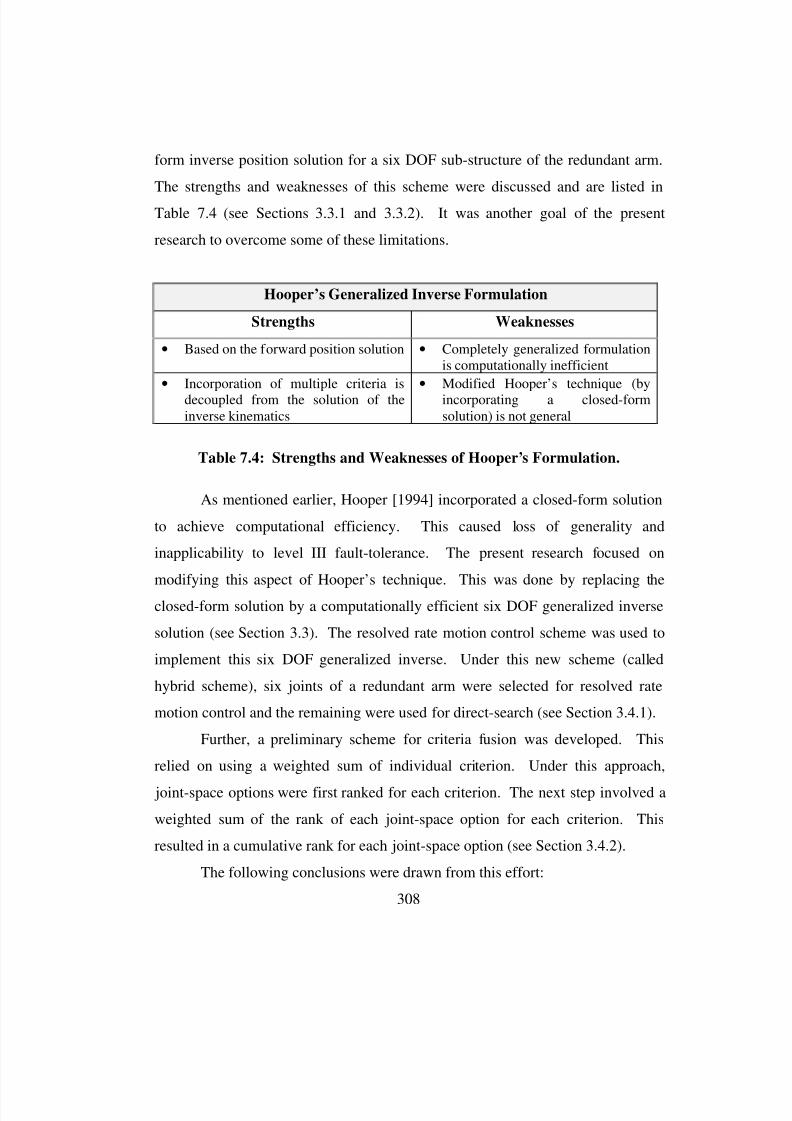
8/3/2019 Chetan Kapoor Dissertation
http://slidepdf.com/reader/full/chetan-kapoor-dissertation 332/612
308
form inverse position solution for a six DOF sub-structure of the redundant arm.
The strengths and weaknesses of this scheme were discussed and are listed in
Table 7.4 (see Sections 3.3.1 and 3.3.2). It was another goal of the present
research to overcome some of these limitations.
As mentioned earlier, Hooper [1994] incorporated a closed-form solution
to achieve computational efficiency. This caused loss of generality and
inapplicability to level III fault-tolerance. The present research focused on
modifying this aspect of Hooper’s technique. This was done by replacing the
closed-form solution by a computationally efficient six DOF generalized inverse
solution (see Section 3.3). The resolved rate motion control scheme was used to
implement this six DOF generalized inverse. Under this new scheme (called
hybrid scheme), six joints of a redundant arm were selected for resolved rate
motion control and the remaining were used for direct-search (see Section 3.4.1).
Further, a preliminary scheme for criteria fusion was developed. This
relied on using a weighted sum of individual criterion. Under this approach,
joint-space options were first ranked for each criterion. The next step involved a
weighted sum of the rank of each joint-space option for each criterion. This
resulted in a cumulative rank for each joint-space option (see Section 3.4.2).
The following conclusions were drawn from this effort:
Hooper’s Generalized Inverse Formulation
Strengths Weaknesses
• Based on the forward position solution • Completely generalized formulationis computationally inefficient
• Incorporation of multiple criteria isdecoupled from the solution of theinverse kinematics
• Modified Hooper’s technique (byincorporating a closed-formsolution) is not general
Table 7.4: Strengths and Weaknesses of Hooper’s Formulation.
8/3/2019 Chetan Kapoor Dissertation
http://slidepdf.com/reader/full/chetan-kapoor-dissertation 333/612
309
• A practical and generalized implementation of a multi-criteria inverse
kinematics problem was achieved. This was demonstrated in real-time on a
seven DOF robot. In this case, the application demonstrated a 170-times
performance improvement over the direct-search technique that was initially
proposed by Hooper [1994] (see Section 3.5).
• The layout of the developed scheme supports level III fault-tolerance.
• The weighted sum technique for criteria fusion can lead to ambiguities. This
happens when a two or more joint-space options have the same overall rank.
This conflict can be resolved using improved criteria normalization with
direct operator intervention.
Further work that needs to be done in developing the hybrid generalized
inverse scheme is as follows:
• The selection of the full rank sub-matrix of the Jacobian matrix for the
computation of the sub-structure inverse should be optimized. Currently, this
selection is arbitrary. A six joint sub-structure of the Jacobian could be
selected by computing the determinant of all the possible full rank Jacobian
sub-matrices. After this, the Jacobian sub-matrix that has the highest
determinant should be selected. However, the determinant is not a good
measure of the distance from a singularity. As an improvement to this, it
would be better to base the selection of the Jacobian sub-matrix by using the
condition number that is computed through Gaussian elimination. The
condition number is a better measure of the distance from singularity than the
determinant. However, the computation of the condition number or
determinant of all possible full-rank sub-matrices of the Jacobian matrix can
be computationally inefficient. Another means of finding the best sub-matrix
of the Jacobian is by conducting a Singular Value Decomposition (SVD) of
the Jacobian matrix and finding the best six constraint equations. This would
8/3/2019 Chetan Kapoor Dissertation
http://slidepdf.com/reader/full/chetan-kapoor-dissertation 334/612
310
be a “one-shot” approach as compared to computing the determinant (or
condition number) for all possible full rank sub-matrices of the Jacobian
matrix.
• The second area that needs further work is level III fault-tolerance. The
current algorithm and its implementation support level III fault-tolerance.
However this has not been tested and debugged. Further work needs to be
done to make this operational and robust.
• The weighted sum technique for criteria fusion was seen to have limitations.
Many of these limitations can be overcome by improving the development of
criteria normalization. A weighted sum of the normalized criterion values
would result in an improved selection of the best joint-space option
7.1.3. Summary and Conclusions of the Environment Selection
The focus of Chapter Four was to discuss the process involved in the
selection of the software development, execution, and test environment. This
included computer hardware, interfacing hardware, robotic hardware, software
development tools, programming languages, design methodology,
communications hardware, and architecture and organization of the software and
the hardware.
The approach taken for environment selection involved the individual
selection of systems that made up the development, execution, and test
environment. This approach was taken even though it was known that individual
system selection was not independent of each other. However, by individually
selecting systems, a clearer picture of what was best was gained. After the
identification of the best sub-system entities, iteration was used to select entities
for all the sub-systems. A summary of the final selected environment is given in
Table 7.5.
8/3/2019 Chetan Kapoor Dissertation
http://slidepdf.com/reader/full/chetan-kapoor-dissertation 335/612
311
In addition to the selection of the development and execution
environment, software was also developed for manual controller integration. This
was possible because the integration of manual controllers required minimal
effort. This was due to the distributed and modular architecture of OSCAR.
Secondly, the OSCAR software architecture could be tested and could be used to
evaluate and study various manual controllers. A distributed approach was taken
for manual controller integration as opposed to centralized control (see Section
4.5). Ethernet was used as the hardware medium for inter-computer
communication. The software used for the communication relied on TCP sockets
(see Section 4.5).
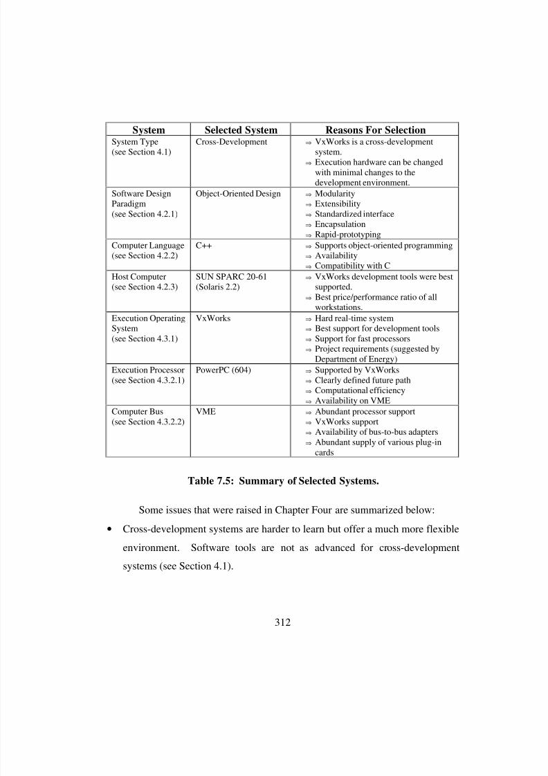
8/3/2019 Chetan Kapoor Dissertation
http://slidepdf.com/reader/full/chetan-kapoor-dissertation 336/612
312
Some issues that were raised in Chapter Four are summarized below:
• Cross-development systems are harder to learn but offer a much more flexible
environment. Software tools are not as advanced for cross-development
systems (see Section 4.1).
System Selected System Reasons For SelectionSystem Type(see Section 4.1)
Cross-Development ⇒ VxWorks is a cross-developmentsystem.
⇒ Execution hardware can be changedwith minimal changes to thedevelopment environment.
Software DesignParadigm(see Section 4.2.1)
Object-Oriented Design ⇒ Modularity⇒ Extensibility⇒ Standardized interface⇒ Encapsulation⇒ Rapid-prototyping
Computer Language(see Section 4.2.2)
C++ ⇒ Supports object-oriented programming⇒ Availability⇒ Compatibility with C
Host Computer(see Section 4.2.3)
SUN SPARC 20-61(Solaris 2.2)
⇒ VxWorks development tools were bestsupported.
⇒ Best price/performance ratio of allworkstations.
Execution OperatingSystem(see Section 4.3.1)
VxWorks ⇒ Hard real-time system⇒ Best support for development tools⇒ Support for fast processors⇒ Project requirements (suggested by
Department of Energy)
Execution Processor(see Section 4.3.2.1)
PowerPC (604) ⇒ Supported by VxWorks⇒ Clearly defined future path⇒ Computational efficiency⇒ Availability on VME
Computer Bus(see Section 4.3.2.2)
VME ⇒ Abundant processor support⇒ VxWorks support⇒ Availability of bus-to-bus adapters⇒ Abundant supply of various plug-in
cards
Table 7.5: Summary of Selected Systems.

8/3/2019 Chetan Kapoor Dissertation
http://slidepdf.com/reader/full/chetan-kapoor-dissertation 337/612
313
• The availability of PowerPC processors has not been as rapid as forecasted. A
viable alternative for the processor of the execution environment is the
Pentium family of processors from Intel (see Section 4.3.2.1).
• The suitability of Windows NT for real-time control needs to be studied.
Windows NT is a soft-real-time system. This means that Windows NT allows
for preemptive execution of parallel tasks but does not guarantee interrupt
latency bounds (approximately six microseconds for VxWorks).
• A SUN workstation was selected as the computer for the development
environment. A Windows NT-based PC could offer a cheaper and equally
powerful option at this time (July, 1996).
7.1.4. Summary and Conclusions of the Abstraction Development
Chapter Five presented the core of this research. This involved the
software component development process (see Section 5.2) and the details of all
the components that were developed as a part of this research (see Section 5.3).
The software development process was divided into three steps. These were
analysis, design, and implementation. Analysis involves the study of the domainand the identification of the key identities, their functionality, and their
relationships (see Section 5.2.1). The next step (design) involves the generation
of implementation level specifications for the entities identified in the analysis
phase (see Section 5.2.2). The last step is the implementation and testing (see
Section 5.2.3) of the entities. There is communication back-and-forth between
the three steps of the development process.
An analysis of the operational software domain of advanced robotics led
to the identification of sub-domains. Additional domains were also identified.
This included domains whose design was necessary to support the development
of the robotics sub-domains. Other domains were developed purely from a
software engineering view point. These domains supported software components

8/3/2019 Chetan Kapoor Dissertation
http://slidepdf.com/reader/full/chetan-kapoor-dissertation 338/612
314
that would facilitate software development (see Section 5.3). A summary of the
selected domains and their functionality is listed in Table 7.6.
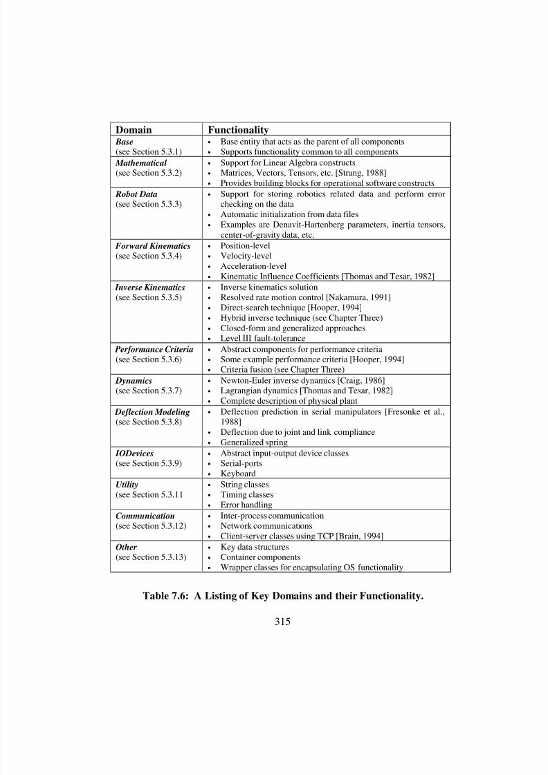
8/3/2019 Chetan Kapoor Dissertation
http://slidepdf.com/reader/full/chetan-kapoor-dissertation 339/612
315
Domain Functionality Base(see Section 5.3.1)
• Base entity that acts as the parent of all components• Supports functionality common to all components
Mathematical (see Section 5.3.2)
• Support for Linear Algebra constructs• Matrices, Vectors, Tensors, etc. [Strang, 1988]• Provides building blocks for operational software constructs
Robot Data(see Section 5.3.3)
• Support for storing robotics related data and perform errorchecking on the data
• Automatic initialization from data files• Examples are Denavit-Hartenberg parameters, inertia tensors,
center-of-gravity data, etc.
Forward Kinematics(see Section 5.3.4)
• Position-level• Velocity-level• Acceleration-level• Kinematic Influence Coefficients [Thomas and Tesar, 1982]
Inverse Kinematics(see Section 5.3.5)
• Inverse kinematics solution• Resolved rate motion control [Nakamura, 1991]• Direct-search technique [Hooper, 1994]• Hybrid inverse technique (see Chapter Three)• Closed-form and generalized approaches• Level III fault-tolerance
Performance Criteria(see Section 5.3.6)
• Abstract components for performance criteria• Some example performance criteria [Hooper, 1994]• Criteria fusion (see Chapter Three)
Dynamics(see Section 5.3.7)
• Newton-Euler inverse dynamics [Craig, 1986]• Lagrangian dynamics [Thomas and Tesar, 1982]• Complete description of physical plant
Deflection Modeling(see Section 5.3.8)
• Deflection prediction in serial manipulators [Fresonke et al.,1988]
• Deflection due to joint and link compliance• Generalized spring
IODevices(see Section 5.3.9)
• Abstract input-output device classes• Serial-ports• Keyboard
Utility(see Section 5.3.11
• String classes• Timing classes• Error handling
Communication(see Section 5.3.12)
• Inter-process communication• Network communications• Client-server classes using TCP [Brain, 1994]
Other(see Section 5.3.13)
• Key data structures• Container components• Wrapper classes for encapsulating OS functionality
Table 7.6: A Listing of Key Domains and their Functionality.
8/3/2019 Chetan Kapoor Dissertation
http://slidepdf.com/reader/full/chetan-kapoor-dissertation 340/612
316
The domains listed in Table 7.6 were further comprised of sub-domains
and software components (C++ classes). These components were connected to
each other through inheritance and containment relationships. Lessons were
acquired regarding domain analysis, design, and management of the software
development process. These are discussed in the following sub-sections.
7.1.4.1. Domain Analysis
A detailed domain analysis is key to the successful design of software.
While conducting this analysis, heed should be given to the current (actual)
functionality desired from the components and the forecasted functionality. The
architecture of the components should be designed to support future additions and
modifications. This is crucial when the domain is based on abstract constructs
and is not fully developed. An example of this is the Performance Criteria
domain that was developed as a part of this research. This domain development
took place keeping in mind that there still was not a fully developed technique for
criteria normalization. In future, an applications developer should be able to
make criteria normalization enhancements with minimal redesign and
implementation.
7.1.4.2. Abstraction Design
The abstraction development process came to the basic conclusion of
“design in parts.” This philosophy has been stressed by designers in all fields.
The adoption of this approach in the component development process stressed the
importance of interface development and specification, and the break down of the
components into sub-components. The granularity of a component was based on
the following “rules of thumb”:
• The interface for a component should fit on a three-by-five inch postcard
[Coplien, 1994].

8/3/2019 Chetan Kapoor Dissertation
http://slidepdf.com/reader/full/chetan-kapoor-dissertation 341/612
317
• A component that is an aggregation of other components will be in general
less efficient than a component that provides all its functionality. In areas
where the real-time constraints are stringent, this might be desired. However,
it was realized that breakdown of components offers long-term hidden
advantages of maintainability and reusability. Note that, the decreased
efficiency of an aggregated component will be counteracted by the
advancement in processor technology.
• A component may need to support specific functionality that would not be
needed anywhere else. In this case, it would be appropriate to build that
functionality into the component rather than making a separate entity to
support that functionality. An example explains this scenario. Consider a
software component that is used to read data from a digital bus. The bus
being used here is proprietary and it will not have any future applications. In
the design of the component in question, a more efficient design may be
achieved by embedding the bus-protocol inside the data reading component.
It should be noted that in such scenarios the developer should carefully weigh
the advantages of embedding functionality as compared to modularizing the
functionality.
Software reuse is achieved in object-oriented design through inheritance
and parameterized data types (see Section 2.5.2). Inheritance is successfully used
by incorporating dynamic binding. Under dynamic binding, the correct
functionality is automatically invoked based on the type of the object. Dynamic
binding is achieved in C++ using a mechanism called virtual methods (see
Section 2.5.1.2.5). A call to a virtual function is more expensive (in time) than a
call to an ordinary method. Additionally, virtual methods cannot be inlined to
improve efficiency. In this research, virtual methods were used infrequently.
Their use was based on how critical it would be in the future to modify a certain

8/3/2019 Chetan Kapoor Dissertation
http://slidepdf.com/reader/full/chetan-kapoor-dissertation 342/612
318
method. The use of virtual methods was especially limited in areas of hardware
interfacing were deterministic performance was desired.
In a good design, components should have alternative means of
demonstrating their functionality. This aspect was even more crucial for this
research as the software architecture was expected to cut down program
development time and also be applicable to real-time control. One means of
reducing program development time was by using an intuitive (perhaps less
efficient) interface. This interface relied on operator overloading. However, for
real-time control the requirement of efficiency was crucial. This conflict was
resolved by having two different interfaces wherever possible. One interface was
designed for ease of use while the other offered computational efficiency.
An analysis of the application domain created the functional
specifications. The analysis also involved an understanding of possible future
applications of a component. From experience gained through this research, it
was realized that better component design could be achieved by designing them in
isolation. The interface of a component should not be biased towards an
application. This can be achieved by avoiding focus on applications of acomponent while designing it. The focus should be on the functionality of the
component and the best way to expose the functionality. Application specific
interface modifications can be made by developers using any of the reusability
techniques.
7.1.4.3. Organization
Consistency in style and organization of source code increases the
availability of the software and is essential to achieve software reuse. The
software development guidelines developed for this research (see Appendix A)

8/3/2019 Chetan Kapoor Dissertation
http://slidepdf.com/reader/full/chetan-kapoor-dissertation 343/612
319
added consistency to the programming style. The source code was organized
using a directory structure (see Section C.3.3) that was parallel to the layout of the
various sub-domains of operational software. It is essential that all developers
that add to this software architecture follow the software development guidelines.
This reduces the effect of individual idiosyncrasies and gives a uniform look and
feel to the system.
The availability of software and its successful release is further dependent
on the configuration management that is in place. The current setup of the
configuration management relies on makefiles and source code control (see
Section C.3.4). Further work needs to be done in this area for better control over
the development and release process.
7.1.5. Summary and Conclusions of the Demonstrations
The purpose of Chapter Six was two-fold. First was the demonstration of
the OSCAR architecture by developing various applications. These applications
demonstrated all aspects of OSCAR. That is, the generalized software
architecture, reusability via inheritance and aggregation, real-time control and
simulation support, manual controller integration, and the development,
execution, and test environment (see Sections 6.2.1 to 6.2.8). In essence, these
applications demonstrated OSCAR’s achievement of all the research goals that
were proposed in Chapter One (see Section 1.2).
The other goal of this chapter was to discuss the validation process for this
research. In the research objectives it was proposed that OSCAR would cut
program development time by 50%. Experiments were conducted with OSCAR
to test this hypothesis (see Section 6.3.1). These experiments involved eight
experimenters. A set of ten experiments were designed in increasing order of
complexity. Seven of the experimenters conducted the ten experiments. The
other experimenter had significant previous robotic software experience and used
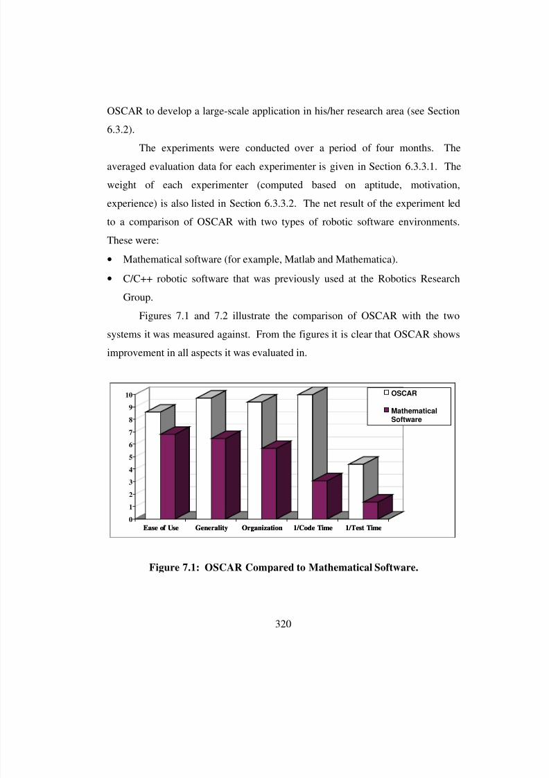
8/3/2019 Chetan Kapoor Dissertation
http://slidepdf.com/reader/full/chetan-kapoor-dissertation 344/612
320
OSCAR to develop a large-scale application in his/her research area (see Section
6.3.2).
The experiments were conducted over a period of four months. The
averaged evaluation data for each experimenter is given in Section 6.3.3.1. The
weight of each experimenter (computed based on aptitude, motivation,
experience) is also listed in Section 6.3.3.2. The net result of the experiment led
to a comparison of OSCAR with two types of robotic software environments.
These were:
• Mathematical software (for example, Matlab and Mathematica).
• C/C++ robotic software that was previously used at the Robotics Research
Group.
Figures 7.1 and 7.2 illustrate the comparison of OSCAR with the two
systems it was measured against. From the figures it is clear that OSCAR shows
improvement in all aspects it was evaluated in.
Ease of Use Generality Organization 1/Code Time 1/Test Time
0
1
2
3
4
5
6
7
8
9
10
Ease of Use Generality Organization 1/Code Time 1/Test Time
OSCAR
MathematicalSoftware
Figure 7.1: OSCAR Compared to Mathematical Software.
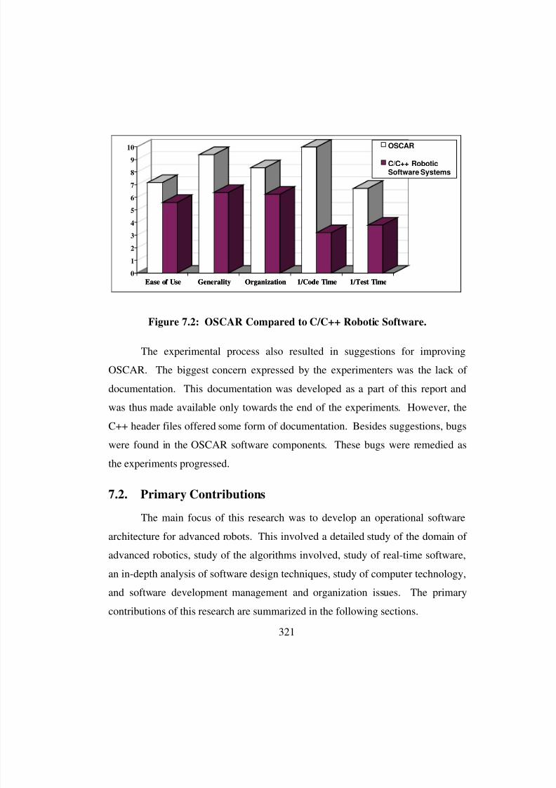
8/3/2019 Chetan Kapoor Dissertation
http://slidepdf.com/reader/full/chetan-kapoor-dissertation 345/612
321
The experimental process also resulted in suggestions for improving
OSCAR. The biggest concern expressed by the experimenters was the lack of
documentation. This documentation was developed as a part of this report and
was thus made available only towards the end of the experiments. However, the
C++ header files offered some form of documentation. Besides suggestions, bugs
were found in the OSCAR software components. These bugs were remedied as
the experiments progressed.
7.2. Primary Contributions
The main focus of this research was to develop an operational software
architecture for advanced robots. This involved a detailed study of the domain of
advanced robotics, study of the algorithms involved, study of real-time software,
an in-depth analysis of software design techniques, study of computer technology,
and software development management and organization issues. The primary
contributions of this research are summarized in the following sections.
Ease of Use Generality Organization 1/Code Time 1/Test Time0
1
2
3
4
5
6
7
8
9
10
Ease of Use Generality Organization 1/Code Time 1/Test Time
OSCAR
C/C++ RoboticSoftware Systems
Figure 7.2: OSCAR Compared to C/C++ Robotic Software.
8/3/2019 Chetan Kapoor Dissertation
http://slidepdf.com/reader/full/chetan-kapoor-dissertation 346/612
322
7.2.1. Generalized Inverse and Criteria Fusion
This research contributed to the area of criteria-based inverse kinematics.An extension to Hooper’s [1994] technique was developed. This technique was
completely generalized and supported Level III fault-tolerance. Additionally, a
preliminary technique for criteria fusion was developed. The limitations of this
technique basically stressed the need for criteria normalization. The algorithm
developed as a part of this research when combined with the OSCAR architecture
offers an excellent framework and environment for research in level III fault-
tolerance and criteria-based decision making. The developed algorithm was
demonstrated in real-time on a seven DOF arm using three criterion and criteria
fusion. In this case, the application demonstrated a 170-times performance
improvement over Hooper’s [1994] direct-search technique.
7.2.2. OSCAR Architecture
An Operational Software Architecture for Advanced Robotics (OSCAR)
was developed. This framework showed improvement over previously used
robotic software architectures. The improvement shown by OSCAR whencompared to mathematical software is shown in Table 7.7.
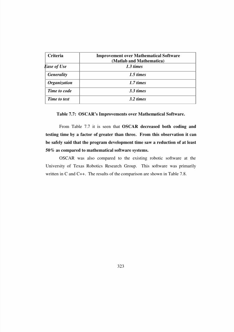
8/3/2019 Chetan Kapoor Dissertation
http://slidepdf.com/reader/full/chetan-kapoor-dissertation 347/612
323
From Table 7.7 it is seen that OSCAR decreased both coding and
testing time by a factor of greater than three. From this observation it can
be safely said that the program development time saw a reduction of at least
50% as compared to mathematical software systems.
OSCAR was also compared to the existing robotic software at the
University of Texas Robotics Research Group. This software was primarily
written in C and C++. The results of the comparison are shown in Table 7.8.
Criteria Improvement over Mathematical Software
(Matlab and Mathematica)
Ease of Use 1.3 times
Generality 1.5 times
Organization 1.7 times
Time to code 3.3 times
Time to test 3.2 times
Table 7.7: OSCAR’s Improvements over Mathematical Software.
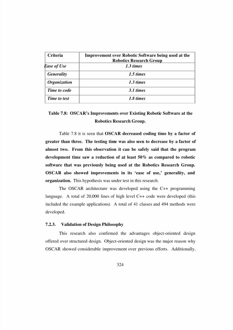
8/3/2019 Chetan Kapoor Dissertation
http://slidepdf.com/reader/full/chetan-kapoor-dissertation 348/612
324
Table 7.8 it is seen that OSCAR decreased coding time by a factor of
greater than three. The testing time was also seen to decrease by a factor of
almost two. From this observation it can be safely said that the program
development time saw a reduction of at least 50% as compared to robotic
software that was previously being used at the Robotics Research Group.
OSCAR also showed improvements in its ‘ease of use,’ generality, and
organization. This hypothesis was under test in this research.
The OSCAR architecture was developed using the C++ programming
language. A total of 20,000 lines of high level C++ code were developed (this
included the example applications). A total of 41 classes and 494 methods were
developed.
7.2.3. Validation of Design Philosophy
This research also confirmed the advantages object-oriented design
offered over structured design. Object-oriented design was the major reason why
OSCAR showed considerable improvement over previous efforts. Additionally,
Criteria Improvement over Robotic Software being used at the
Robotics Research Group
Ease of Use 1.3 times
Generality 1.5 times
Organization 1.3 times
Time to code 3.1 times
Time to test 1.8 times
Table 7.8: OSCAR’s Improvements over Existing Robotic Software at the
Robotics Research Group.
8/3/2019 Chetan Kapoor Dissertation
http://slidepdf.com/reader/full/chetan-kapoor-dissertation 349/612
325
the advantages of distributed control (as seen from manual controller integration
in Section 4.5) over centralized control were validated.
7.2.4. Development, Execution, and Test Environment
Another contribution of this research was that it provided a framework for
robotic software development. This framework included, software development
tools, software execution environment, and robotic devices for software testing.
A completely integrated and yet distributed environment was developed that
supported real-time control, simulation, manual controllers, and a variety of
robotic devices. Moreover, the effort put into software organization and
management greatly enhanced the availability of OSCAR. Additionally, software
development guidelines were put in place for the Robotics Research Group.
7.2.5. Developer Training
It was realized during the course of this research that the real worth of
OSCAR can only be realized if it can be used to solve “real-world” problems.
This would only be possible if applications developers were trained in the use of
OSCAR. The experiments conducted as a part of this research (see Section 6.3)
not only served the purpose of validating this research, but also were a vehicle for
developer training. Additionally, example application programs were developed
using the OSCAR architecture to facilitate developer training (see Section 6.2).
7.2.6. Management
Besides core research contributions, a major effort was spent in just
keeping “things up and running.” The OSCAR architecture incorporated the
Robotics Research Dual Arm, four manual controllers, four computers, three
operating systems, and multiple users. The presence of many components and
multiple users made the management process complex. However, due to the
8/3/2019 Chetan Kapoor Dissertation
http://slidepdf.com/reader/full/chetan-kapoor-dissertation 350/612
326
distinct and distributed nature of these systems, OSCAR was never unoperational.
If the physical robot was not working, a simulation could be used for program
development. If VxWorks was unavailable, control program development could
still take place on the Solaris system.
In summary, a major effort was spent on just managing and nurturing this
system through its infancy. Finally, at this point of time (August, 1996) the
system has reached stability and all the problems are well understood. Most of
these problems are robotic hardware related and are being remedied.
This research would not have been possible without the team-spirit shown
by the people involved in the development of OSCAR. These included people
who were developing applications using OSCAR, developing hardware for use in
the OSCAR environment, and people involved in making high-level decisions
regarding OSCAR’s direction. This effort was a success due to the motivation,
hard-work, and team-spirit of everyone involved.
7.3. Supporting Technologies for Operational Software
OSCAR offers to the robotic software developer an environment that canbe used to develop control programs. OSCAR by itself does not offer a complete
system for robotic application development. Other technologies have to be
developed for the enhancement, use, and support of OSCAR. There are some
areas of robotic operational software that OSCAR does not currently support.
These need to be developed to enhance OSCAR. Other areas need to be
developed that will allow the use of OSCAR. For example, a real-time control
layer needs to be developed. This layer will be used by OSCAR to interface with
actual physical hardware (a preliminary real-time control layer was developed by
Rackers [1996] for this research). Other areas need to be developed to support
the software components that OSCAR presents. For example, OSCAR supports
the generalized inverse formulation. However, as high precision jobs require an
8/3/2019 Chetan Kapoor Dissertation
http://slidepdf.com/reader/full/chetan-kapoor-dissertation 351/612
327
exact model of the system, the exact physical parameters of the system are
desired. For this to be possible, robot metrology needs to be addressed. These
technology areas that need development are discussed in detail in the following
sections.
7.3.1. Computer Hardware
OSCAR is a software architecture. It uses computer hardware for
program execution. The design of OSCAR has been based on the assumption
that, computer hardware will continue to improve at the rate predicted (a 100+
improvement in the next five years as predicted by Hooper [1994]). From
industry trends it is seen that the price/performance ratio of computers is steadily
increasing. The performance of personal computers is forecasted at 800 MIPS by
the year 2000 (see Section 2.7). This is encouraging for OSCAR development.
OSCAR will also gain from the advancement in computer architecture. General
purpose multiple processor PC’s are currently available. The advantages of using
a multiprocessor architecture will become evident as the support for multicriteria
decision making increases. In essence, computer hardware is a technology that is
driven by the consumer industry and will greatly improve the performance and
availability of OSCAR.
7.3.2. Operating Systems
An operating system is the software that interfaces with the hardware of a
computer and encapsulates its functionality. All modern day computers come
equipped with an operating system. In fact, most computers offer its users a
choice of operating systems. For example, an Intel-based PC can support
Windows, Windows NT, LynxOS (real-time UNIX), SCO UNIX, etc.
The new generation of operating systems being developed all support
parallel execution of software and also have extensions for symmetric
8/3/2019 Chetan Kapoor Dissertation
http://slidepdf.com/reader/full/chetan-kapoor-dissertation 352/612
328
multiprocessing (SMP). An SMP operating system is used in multiprocessor
systems. In a SMP system, a copy of the operating system is supported by each
processor. No processor is the master in such a system. Software programs can
be developed using the SMP systems that allow for automatic allocation of
parallel tasks to different processors. Operating systems like Windows NT and
OS/2 have even further simplified the development of parallel programs. A
parallel program developed for Windows NT will run on a single processor
system or will automatically use all the available processors if run on a multiple
processor hardware [Brain, 1995]. This allows for portability and simplified
program development.
All major operating systems are now 32 bit. This means that data is
processed by these operating systems in blocks of size 32 bit. UNIX workstations
are currently moving to a 64 bit operating system (an example is IRIX 6.0 from
Silicon Graphics). Robotic computations, which are primarily floating point,
greatly benefit from the move to 32 bit and 64 bit operating systems (floating
point numbers are 32 bit or 64 bit in size).
Operating systems have also shown an improvement in their support forreal-time program development. Real-time program development is based on
parallel software execution, priority-based allocation of resources, and
deterministic interrupt handling. Currently, commercial operating systems like
Windows NT and OS/2 do not support real-time software development, though
real-time versions of UNIX are available. The future will see a move towards the
use of commercial operating systems because of their high price/performance
ratio. This will become feasible as these operating systems will further develop
their support for real-time program development.
In summary, operating system technology is also consumer industry
driven and will continue to improve. More will be expected of operating systems.
8/3/2019 Chetan Kapoor Dissertation
http://slidepdf.com/reader/full/chetan-kapoor-dissertation 353/612
329
This will allow OSCAR to focus more on robotic software. Utilities for efficient
program development and execution will be a part of the operating system.
7.3.3. Communications
Communications involves data exchange between two computers or
within a computer. Different types of communication mechanisms are used based
on the application. For example, the communication between the system
controller of a robot and the servo controllers is generally tightly coupled and
uses a high-speed bus [Aalund et al., 1993]. Bus technology has seen consistent
improvement. For example, the XT bus used in personal computers in the early
1980’s had a bandwidth of 800 Kbytes/second. Currently, the Turbo Channel bus
used in Digital workstations has a bandwidth of 98,000 Kbytes/second. This is a
122-time improvement. This improvement in bus technology bodes well for
distributed operational software.
Besides the development of bus technology, the robotic industry has seen
the development of standard protocols for communication. Again, these
communications are at two levels. First is the communication protocol for tightly
coupled machines (an example is the coupling between the system controller and
the servo controllers). An example of this is the SERCOS standard. The Serial
Real-time Communication System (SERCOS) standard provides a basis so that
manufacturers can build components (control units, drives, etc.) that can operate
trouble-free with components made by other manufacturers. Thus, SERCOS
defines a uniform interface for dialog between digital drives and control units of
numerically controlled machines [Puls, 1994]. The proliferation of
communication standards gives the system developer a bigger pool to choose
from. Moreover it is seen that a majority of the communication protocols are
being supported on different bus architectures. This again bodes well for the
robotic control system developer.
8/3/2019 Chetan Kapoor Dissertation
http://slidepdf.com/reader/full/chetan-kapoor-dissertation 354/612
330
The second form of communication protocol is used between computers
that are loosely coupled. An example of this is two computers on the Internet.
Generally, this type of communication cannot be used for real-time control. The
biggest application of this form of communication is in factory automation
systems. A robotic system controller in a “real” application has to coordinate
with other machines and has to continuously exchange data with them. This type
of communication protocol was used in this research for manual controller
integration and for distributed computing. Various standard software libraries are
currently available that allow world-wide communication between computers.
An example of this is the Transmission Control Protocol (TCP). TCP allows the
transmission and receiving of packets of data between different computers. Using
TCP, data exchange software has been developed that allows for a program to
execute on multiple computers. One such standard is the Common Object
Request Brokerage Agent (CORBA) [Burchard and Feddema, 1996]. CORBA
allows for exchanging objects (from object-oriented programming) between
computers. When an object is passed from one computer to another, the receiving
computer can operate on this object as if it was created over there. Thistechnology simplifies distributed program development. Also, the CORBA
standard hides the differences between the hardware architecture of the computers
exchanging data. An example of this is when data is exchanged between a
Motorola-based computer and an Intel-based computer. In this case the byte
order of the data has to be swapped.
Basically, bus technology, communication protocols, and object exchange
software have shown considerable improvement in the past few years. A big
reason for this is the increase in processor speeds and emergence of object-
oriented design. Robotic software should now be designed to take advantage of
these technologies. This has not been the case in the past. Previously robotic
controllers were specifically developed for each robot. This included the
8/3/2019 Chetan Kapoor Dissertation
http://slidepdf.com/reader/full/chetan-kapoor-dissertation 355/612
331
hardware, operating system, communication protocols, and robot programming
languages. The time has come for robotic industry to drive itself from the best in
commercially available technology rather than trying to “patch-up” old
technology to meet customer demands.
7.3.4. Configuration Management Tools for Software
The configuration management of software has one major goal. This is to
have only one version of source code. The configuration management system
should be able to use this source code and build shippable versions for different
platforms and different applications. For example, if an OSCAR control program
is needed for controlling a six DOF arm, with deflection compensation, using a
Windows NT PC, the configuration management should be able to access and
combine the right components to generate an executable program.
The development of OSCAR took place in an academic environment. In
such an environment there are no product release dates, product versions, and
product shipments. For OSCAR to be commercially viable, it is necessary to
develop a configuration management system for software development and
shipment. This technology is well understood by the software industry and tools
are available for configuration control.
OSCAR development environment currently supports some configuration
management. OSCAR can currently be compiled for three operating systems.
These are VxWorks, Solaris, and Windows NT. This is all automated using
makefiles [Oram and Talbott, 1995]. Version control in OSCAR is being
currently implemented using Source Code Control System (SCCS) [Bolinger and
Bronson, 1995].
In summary, configuration control is necessary for development of a
commercial product that caters to different applications. Software tools for
configuration management are commercially available and can be easily

8/3/2019 Chetan Kapoor Dissertation
http://slidepdf.com/reader/full/chetan-kapoor-dissertation 356/612
332
incorporated into the OSCAR development environment. Makefile’s and SCCS
are already incorporated in OSCAR. It is seen though that a majority of large
software companies have developed their own configuration control system (for
example, National Instruments). This was done because the commercial systems
were not adaptable to individual needs. This problem will go away in the future.
This is because the software industry is also moving towards “agile
manufacturing.” Applications developers will be able to get software components
from different vendors and assemble them to satisfy their application needs. This
trend bodes well for the future of OSCAR.
7.3.5. Graphical User Interface
A graphical user interface (GUI) is used to provide the man-machine
interface. The OSCAR architecture constitutes the middle layer of robotic
software. The layer above this is the man-machine interface. This includes the
robot programming language. Current trends in industry show a move towards
visual programming. These programming systems allow the applications
developer to generate control programs using a GUI. This approach to program
development has also been used in robotics [Kapoor, 1992]. Additionally, the
robot controller available from Cimetrix Incorporated [1996] also supports a GUI
based robot programming environment. LabView from National Instruments
[1996] is another example of a visual programming environment. It allows the
user to graphically connect sub-systems to generate application programs.
Extensive work has been done in the research community in developing
graphical user interfaces for man-machine software. Some examples of these
systems were discussed in Chapter Two (Sections 2.6.2.2 to 2.6.2.5). OSCAR
could be combined with these systems to offer a complete solution. However, the
robotic GUI systems developed in academia are generally based on proprietary
software environments. This limits their portability and future growth potential.
8/3/2019 Chetan Kapoor Dissertation
http://slidepdf.com/reader/full/chetan-kapoor-dissertation 357/612
333
A better approach would be to use a commercial GUI framework and add robotic
specific GUI components to it. An example of this is the LabView software
environment from National Instruments [1996]. This software is the de-facto
industrial standard for instrumentation. LabView is based on visual
programming. In this environment, the application developer connects various
sub-systems graphically. Additionally, LabView provides a rapid-prototyping
environment for GUI development. Support is currently being added to LabView
to assist in factory automation. This includes support for programmable logic
controllers (PLC), various industrial buses, motion control, data-acquisition, etc.
All these technologies are used in robot system integration. In essence, the use of
commercial systems for robot software development is along the lines of this
research, that is, software reuse and incorporation of the latest in commercial
technology.
7.4. Future Work
This section provides a roadmap for future development of robotic
software. This includes the enhancements that have to be made to OSCAR.These enhancements will include the development of new sub-domains within
OSCAR and also the improvement of the current components in OSCAR.
Additional work also needs to be done in the development of the other
layers of software that are involved in system control. These are the man-
machine interface and real-time control.
Besides system control, effort needs to be directed at the development of a
software architecture for actuator level control. A software architecture that
encompasses all possible manual controllers also needs to be developed. Further,
a software system for maintenance of machines needs to be developed.
The previous paragraphs suggested other domains that need development.
Once a large number of components are available to the applications developer,
8/3/2019 Chetan Kapoor Dissertation
http://slidepdf.com/reader/full/chetan-kapoor-dissertation 358/612
334
the next step is the selection and assembly of the components. A software system
needs to be put in place for this purpose.
The ultimate test of a robotic software system would be its applicability to
manufacturing cell control. These manufacturing cells should be based on jigless
and fixtureless manufacturing, reduced integration time, reduced robot
programming time, and a predictable maintenance schedule. Towards the end,
this section addresses some of the issues involved in manufacturing cell
development. The last section provides a time-line for the development of the
technologies that were addressed in this section.
7.4.1. Other Operational Software Domains
OSCAR provides a framework for robotic software development.
OSCAR currently addresses the issues involved in operational software of
advanced robots. Not all domains that are present in operational software were
addressed by OSCAR. The following section discusses the other sub-domains
that need development or enhancements.
7.4.1.1. Obstacle Avoidance
The importance of on-line obstacle detection and avoidance is expected to
increase rapidly in the near future. This is going to become extremely necessary
as manufacturing shifts its focus to an agile system comprised of manufacturing
cells.
The software system for obstacle avoidance consists broadly of two sub-
systems. These are the obstacles and the algorithm for avoiding obstacles. The
obstacle avoidance domain should provide the robotic software developer a
flexible and general means of describing obstacles. The algorithm used for

8/3/2019 Chetan Kapoor Dissertation
http://slidepdf.com/reader/full/chetan-kapoor-dissertation 359/612
335
obstacle avoidance should also be general. These software issues for these two
systems are described below.
7.4.1.1.1. Generalized Obstacle Description
Perry [1995] identified key shapes that constituted an obstacle. These
were cylinders, cones, double-cones, and spheres. All these shapes can be
addressed as a part of an inheritance hierarchy in object-oriented design. New
shapes could also be created by aggregating the existing shapes. A class
hierarchy for these shapes has already been created for 3D graphics software
development (see Appendix D). This class hierarchy could be used to express
obstacles.
Two different types of obstacles will have to be provided. These will be
static obstacles that do not change shape. The design of the software for these
obstacles should be tuned towards a faster computation of the distances of these
obstacles from the robot. The other type of obstacle will be reconfigurable. This
type of obstacle will change its shape and will be used to express systems with
moving parts (for example, another robot). The software for reconfigurable
obstacles should be tuned towards efficient reconfiguration and distance
calculation.
7.4.1.1.2. Generalized Algorithm for Obstacle Avoidance
The preliminary algorithm developed by Perry [1996] for obstacle
avoidance was based on the use of kinematic influence coefficients [Thomas and
Tesar, 1982]. Using these, distance functions were formulated to determine the
distance between a serial robot and obstacles within its workspace. Further, this
algorithm was incorporated into an initial criteria-based decision making scheme.
For a given set of joint-space options that satisfied a particular end-effector
constraint, the obstacle avoidance criterion ranked these options based on the
8/3/2019 Chetan Kapoor Dissertation
http://slidepdf.com/reader/full/chetan-kapoor-dissertation 360/612
336
maximum distance from obstacles. The joint-space option that had the maximum
distance from the obstacle was the selected solution.
This algorithm fits directly into the OSCAR architecture. Components are
already present in OSCAR that support the computation of first and second-order
kinematic influence coefficients. The Performance Criteria domain allows the
efficient creation of new criteria. For the obstacle avoidance criterion, the only
functionality that has to be added will be the calculation of the distance of a robot
from the obstacles. The computation of forward kinematics solution, the ranking
of the joints-space options, and the fusion of criteria will be automatically
handled by OSCAR.
In summary, two steps have to be accomplished for the obstacle avoidance
domain. These are, the development of a class hierarchy to express different
shaped obstacles and the development of an obstacle avoidance criterion.
7.4.1.2. Performance Criteria
The Performance Criteria domain was developed as a part of OSCAR.
However, only three performance criterion were developed. VanDoren [1992] in
his Masters thesis identified twenty-nine different criteria. These criteria need to
be implemented. The implementation of these performance criterion will take
place within the framework provided in the Performance Criteria domain. The
developer will have to only provide the functionality for computing the criterion
value for a particular joint-space option. The functionality for ranking the various
criteria values and for criteria fusion will be common to all performance criteria.
Tables 7.9 to 7.12 list the criteria that need development and the OSCAR
components that they will use. All the new performance criteria components will
be derived from the RRPerformanceCriteria component (see Section 5.3.6.1).
The performance criteria are further divided into geometric, force/torque, kinetic
energy, and compliance. Refer to Hooper [1994] for further details on the

8/3/2019 Chetan Kapoor Dissertation
http://slidepdf.com/reader/full/chetan-kapoor-dissertation 361/612
337
individual criteria. The following sub-sections discuss the various types of
performance criteria and their dependency on OSCAR.
7.4.1.2.1. Geometric Performance Criteria
Table 7.9 shows the various geometric performance criterion. These
criterion are dependent on the first and second-order kinematic influence
coefficients. The RRFKJacobian (see Section 5.3.4.2) and RRFKVelocity (see
Section 5.3.4.4) provide the first-order kinematic influence coefficients. The
RRFKAcceleration (see Section 5.3.4.5) provides the second-order influence
coefficients.
7.4.1.2.2. Force/Torque Performance Criteria
Geometric Performance Criteria OSCAR Components to Use
(all use
RRPerformanceCriteria)
Singularity detection RRFKJacobian
Dexterity RRFKJacobian
Velocity transmission RRFKJacobian, RRFKVelocity
Force and torque transmission RRFKJacobian, RRFKVelocityJacobian Frobenius Norm RRFKJacobian, RRFKVelocity
Rate of change of singularity detection RRFKAcceleration
Rate of change of dexterity criterion RRFKAcceleration
End-effector velocity-induced jointacceleration
RRFKAcceleration
Joint velocity-induced end-effectoracceleration
RRFKAcceleration
Table 7.9: OSCAR Components Required for the Development of Various
Geometric Criteria.
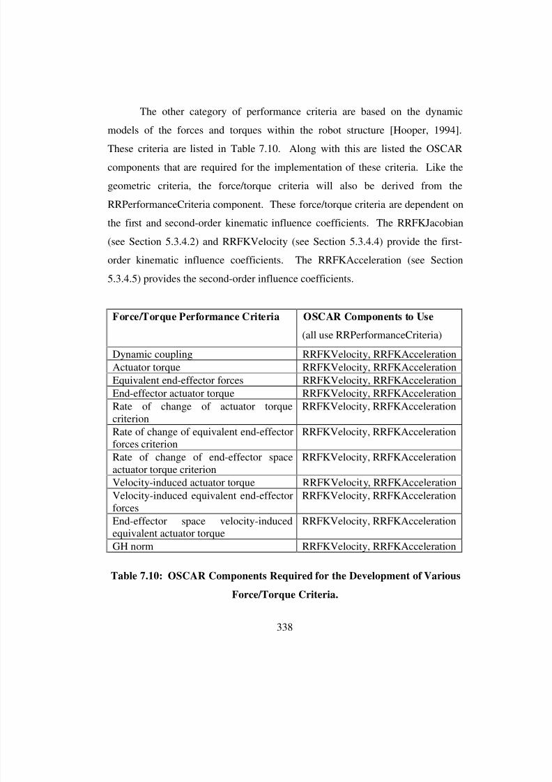
8/3/2019 Chetan Kapoor Dissertation
http://slidepdf.com/reader/full/chetan-kapoor-dissertation 362/612
338
The other category of performance criteria are based on the dynamic
models of the forces and torques within the robot structure [Hooper, 1994].
These criteria are listed in Table 7.10. Along with this are listed the OSCAR
components that are required for the implementation of these criteria. Like the
geometric criteria, the force/torque criteria will also be derived from the
RRPerformanceCriteria component. These force/torque criteria are dependent on
the first and second-order kinematic influence coefficients. The RRFKJacobian
(see Section 5.3.4.2) and RRFKVelocity (see Section 5.3.4.4) provide the first-
order kinematic influence coefficients. The RRFKAcceleration (see Section
5.3.4.5) provides the second-order influence coefficients.
Force/Torque Performance Criteria OSCAR Components to Use
(all use RRPerformanceCriteria)
Dynamic coupling RRFKVelocity, RRFKAcceleration
Actuator torque RRFKVelocity, RRFKAcceleration
Equivalent end-effector forces RRFKVelocity, RRFKAcceleration
End-effector actuator torque RRFKVelocity, RRFKAcceleration
Rate of change of actuator torquecriterion RRFKVelocity, RRFKAcceleration
Rate of change of equivalent end-effectorforces criterion
RRFKVelocity, RRFKAcceleration
Rate of change of end-effector spaceactuator torque criterion
RRFKVelocity, RRFKAcceleration
Velocity-induced actuator torque RRFKVelocity, RRFKAcceleration
Velocity-induced equivalent end-effectorforces
RRFKVelocity, RRFKAcceleration
End-effector space velocity-inducedequivalent actuator torque
RRFKVelocity, RRFKAcceleration
GH norm RRFKVelocity, RRFKAcceleration
Table 7.10: OSCAR Components Required for the Development of Various
Force/Torque Criteria.
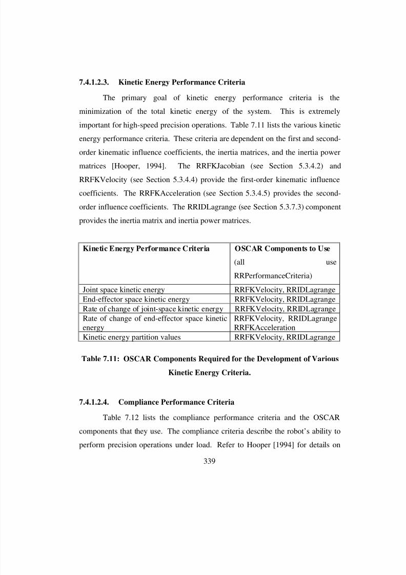
8/3/2019 Chetan Kapoor Dissertation
http://slidepdf.com/reader/full/chetan-kapoor-dissertation 363/612
339
7.4.1.2.3. Kinetic Energy Performance Criteria
The primary goal of kinetic energy performance criteria is theminimization of the total kinetic energy of the system. This is extremely
important for high-speed precision operations. Table 7.11 lists the various kinetic
energy performance criteria. These criteria are dependent on the first and second-
order kinematic influence coefficients, the inertia matrices, and the inertia power
matrices [Hooper, 1994]. The RRFKJacobian (see Section 5.3.4.2) and
RRFKVelocity (see Section 5.3.4.4) provide the first-order kinematic influence
coefficients. The RRFKAcceleration (see Section 5.3.4.5) provides the second-
order influence coefficients. The RRIDLagrange (see Section 5.3.7.3) component
provides the inertia matrix and inertia power matrices.
7.4.1.2.4. Compliance Performance Criteria
Table 7.12 lists the compliance performance criteria and the OSCAR
components that they use. The compliance criteria describe the robot’s ability to
perform precision operations under load. Refer to Hooper [1994] for details on
Kinetic Energy Performance Criteria OSCAR Components to Use
(all use
RRPerformanceCriteria)
Joint space kinetic energy RRFKVelocity, RRIDLagrange
End-effector space kinetic energy RRFKVelocity, RRIDLagrangeRate of change of joint-space kinetic energy RRFKVelocity, RRIDLagrange
Rate of change of end-effector space kineticenergy
RRFKVelocity, RRIDLagrangeRRFKAcceleration
Kinetic energy partition values RRFKVelocity, RRIDLagrange
Table 7.11: OSCAR Components Required for the Development of Various
Kinetic Energy Criteria.
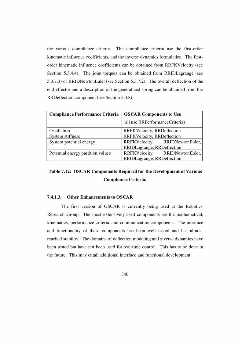
8/3/2019 Chetan Kapoor Dissertation
http://slidepdf.com/reader/full/chetan-kapoor-dissertation 364/612
340
the various compliance criteria. The compliance criteria use the first-order
kinematic influence coefficients, and the inverse dynamics formulation. The first-
order kinematic influence coefficients can be obtained from RRFKVelocity (see
Section 5.3.4.4). The joint torques can be obtained from RRIDLagrange (see
5.3.7.3) or RRIDNewtonEuler (see Section 5.3.7.2). The overall deflection of the
end-effector and a description of the generalized spring can be obtained from the
RRDeflection component (see Section 5.3.8).
7.4.1.3. Other Enhancements to OSCAR
The first version of OSCAR is currently being used at the Robotics
Research Group. The most extensively used components are the mathematical,
kinematics, performance criteria, and communication components. The interface
and functionality of these components has been well tested and has almost
reached stability. The domains of deflection modeling and inverse dynamics havebeen tested but have not been used for real-time control. This has to be done in
the future. This may entail additional interface and functional development.
Compliance Performance Criteria OSCAR Components to Use
(all use RRPerformanceCriteria)
Oscillation RRFKVelocity, RRDeflection
System stiffness RRFKVelocity, RRDeflection
System potential energy RRFKVelocity, RRIDNewtonEuler,RRIDLagrange, RRDeflection
Potential energy partition values RRFKVelocity, RRIDNewtonEuler,RRIDLagrange, RRDeflection
Table 7.12: OSCAR Components Required for the Development of Various
Compliance Criteria.
8/3/2019 Chetan Kapoor Dissertation
http://slidepdf.com/reader/full/chetan-kapoor-dissertation 365/612
341
Under kinematics, software components are provided that can be used for
a criteria-based generalized inverse. These components inherently support level
III fault-tolerance functionality. However, complete testing of the level III fault-
tolerance support is needed. This is currently being accomplished at the Robotics
Research Group.
7.4.2. Other Software Architectures for System Level Control
Besides operational software, there are other areas of system control
software that need development. The two other layers of system control software
are the man-machine interface and the real-time control. The following sections
discuss some of the issues involved and offer suggestions in the development of a
software architecture for these layers.
7.4.2.1. Software Architecture for Man-Machine Interface
The man-machine interface for robots includes the robot programming
language and the GUI for commanding the robot. Academic research has led to
the development of a variety of robot programming languages. These range from
very simple interpreted languages to task-level languages. Standard programming
languages like C, Ada, etc. have also been used for robot programming.
Currently, it is seen that there is no standard for robot programming languages.
Commercially robotic controllers are currently offering the robot programmer
with a choice of robot programming environments. For example, the SC 4000
system controller from Cimetrix Incorporated offers three different environments
for robot programming. One of these is a GUI based robot programming
environment.
The robotic industry has a lot to leverage from the commercial software
industry when it comes to man-machine interfaces. The proliferation of
windows-based operating systems is evident from the boom in the PC market.
8/3/2019 Chetan Kapoor Dissertation
http://slidepdf.com/reader/full/chetan-kapoor-dissertation 366/612
342
The availability of such systems has made available a wide range of GUI
development tools. Additionally, a majority of visual programming environments
are currently available. These environments allow the generation of programs
using a GUI and without writing any code.
The following steps should be taken for the development of a man-
machine interface:
• Commercially available and popular robot programming languages should be
studied. Lessons learned from these robot programming languages should be
used to further develop a teleoperator language to support redundant arms,
decision-making, and fault-tolerance.
• This robot programming language should be incorporated in a commercial
visual programming environment. The visual programming environment that
is selected should be geared toward hardware interfacing and machines.
LabView from National Instruments [1996] is an example of this.
Enhancements should be made to the selected visual programming
environment to add support for advanced robotics.
• The man-machine interface software developed at Sandia National
Laboratories (see Sections 2.6.2.2 to 2.6.2.4) should be reviewed in detail.
Currently, this system is geared more towards standard industrial robots. If
this system is extensibility and portable it could offer a solution for man-
machine interface software.
7.4.2.2. Software Architecture for Real-Time Control
The real-time control layer is the lower-most layer of robotic system
control software. This is the layer which interfaces with external hardware, sends
set-points to the servo controllers, accepts feedback and may be responsible for
running control loops.
8/3/2019 Chetan Kapoor Dissertation
http://slidepdf.com/reader/full/chetan-kapoor-dissertation 367/612
343
A preliminary real-time control layer was developed by Rackers [1996].
This layer is currently used by OSCAR to communicate with physical hardware.
However, this layer is specific to the system being used and does not offer much
extensibility. A reusable and general real-time control layer needs to be
developed. This layer should offer a standard interface to OSCAR. The key
factors to consider while designing this layer are as follows:
• The real-time control layer has to respond to multiple external events. These
events could be random and may occur asynchronously. A parallel execution
environment is best suited to the development of this layer and is supported
by most real-time operating systems. Furthermore, most operating systems
offer tools to simplify parallel program development. An example of this is
the Wind Foundation Classes from WindRiver Systems.
• A major part of the real-time layer is hardware interfacing software. In
general, it is undesirable to communicate with hardware directly. Most
operating systems (for example, Windows NT and UNIX) would actually not
allow an applications program to do this. The safe and correct way to access
hardware is through device drivers. Device drivers provide a uniform
interface to the hardware and also allow for safe access. For example, if a
device driver is being used to access a serial port by one program, another
program would be denied access to the serial port until the first program has
completed its operation. Thus, before the development of real-time control
layer is undertaken, heed should be given to the availability of device drivers.
• Another requirement of the real-time layer is communications and
multiplexing. The system controller generally communicates with the servo
controllers over a high-speed bus. Moreover, the same bus might be used by
more than two devices to communicate. In such a case the communication
has to be multiplexed.
8/3/2019 Chetan Kapoor Dissertation
http://slidepdf.com/reader/full/chetan-kapoor-dissertation 368/612
344
Keeping in mind the above mentioned functionality of the real-time
control layer, a preliminary identification of sub-domains has been done. These
are listed below:
• Class structure for input/output devices. These could be boards, ports,
communication protocols, etc. This class structure should be designed
keeping in mind the portability of the system. The real-time layer should be
able to maintain the same interface when ported to another operating system.
• A class structure for encapsulating the functionality of the operating system
needs to be designed. This would include tasks, synchronization mechanisms
(semaphores, etc.), inter-task communication mechanisms (shared memory,
pipes, mailboxes, etc.). However, the development of this class structure may
not be required as most operating system vendors offer a class library that
encapsulates operating system functionality.
• System controllers for current industrial robots have minimal communication
traffic with the servo controllers. This leads to a simple communications
software architecture. However, advanced robots are going to be
characterized by fault-tolerant actuators. These actuators will have redundant
sensors and will provide a functional map that will allow for their
performance prediction. Information regarding temperature, voltage, current,
torque, etc. will be generated inside the actuator. This information in some
cases will have to be delivered to the system controller in real-time and a high
rate (greater than 100 Hertz). This would put unprecedented demands on the
communication system. The real-time control layer will have to address these
issues.
7.4.3. Software Architectures in Other Domains
OSCAR addressed the software issues involved with system control of
advanced manipulators. The issues involved with servo control of actuators were
8/3/2019 Chetan Kapoor Dissertation
http://slidepdf.com/reader/full/chetan-kapoor-dissertation 369/612
345
not addressed. Further, OSCAR supported software for manual controller
integration. However, a systematic architecture that represented all classes of
manual controllers was not developed. Thus, future work needs to be pursued in
the development of software architectures for actuator control and manual
controllers. This is discussed in the following sections.
7.4.3.1. Reusable Software Architecture for Actuator Level Control
An actuator is a self-contained prime-mover. For example, an electric
motor driven actuator may comprise of a motor, gear-train, sensors, a brake, a
clutch, and also the servo-level control hardware and software. Just as this
research developed an architecture for operational software of advanced robots, a
software architecture for controls of actuators is desired. This architecture should
serve the purpose of a most basic actuator and should be extensible enough to
support advanced actuators that could be used in space. The following paragraph
discuss the key characteristics of advanced actuators [Tesar, 1996]1. This
discussion will provide a preliminary analysis of the problem domain. Based on
this analysis, suggestions will be made regarding the design of the software
architecture.
7.4.3.1.1. Architectural and Functional Analysis of an Advanced Actuator
This section discusses the key functionality of an advanced actuator.
Along with the functionality, architectural issues that will have an impact on the
software architecture are also discussed. This discussion is presented below:
1 Dissertation on high-resolution position sensing system in progress by Brent Nowak at the
Robotics Research Group

8/3/2019 Chetan Kapoor Dissertation
http://slidepdf.com/reader/full/chetan-kapoor-dissertation 370/612
346
• Simple actuators use only one sensor as a basis for control. This is usually
a position sensor (encoder or resolver). Also, these actuators are primarily
based on a simple control scheme such as PID control.
• Advanced actuators will be based on multiple sensors. Varied sensor
information will be essential for implementing advanced non-linear
control schemes such as model-based control. By fusing the sensory
information with an efficient model of the system, higher performance
will be achieved1.
• Enhanced performance will be the key advantage of an advanced actuator.
The same actuator will be able to use the input sensory information and
reconfigure its control scheme to respond to application need. For
example, for high-speed assembly tasks, the control scheme will support
rapid response. For precision jobs, the control scheme will support
disturbance rejection and high-accuracy2.
• Currently, ten different types of sensors are proposed in an advanced
actuator. These sensors along with their key characteristics are listed
below:
a. position up to 22 bit accuracy,
b. velocity advanced tachometer,
c. acceleration accelerometer,
d. torque up to 12 bit accuracy,
e. temperature primarily in motor,
f. vibration to sense wear damage,
g. sound to sense incipient failure,
h. voltage to describe motor operation,
i. current to describe motor operation,
2 Dissertation on actuator control issues in progress by Eric Scott at the Robotics Research Group

8/3/2019 Chetan Kapoor Dissertation
http://slidepdf.com/reader/full/chetan-kapoor-dissertation 371/612
347
j. magnetic field to describe motor operation. [Tesar, 1996]
• Condition-based maintenance will be achieved by these actuators by
comparing an accurate model reference of the actuator with a sensor
reference. This comparison will provide a time-sheet for maintenance3.
• Actuators for space will support fault-tolerance. Fault-tolerance will be
achieved by duality in every active component such as motors, gears,
trains, etc. [Iaconics, 1991].
• As mentioned earlier, an advanced actuator will be sensor intensive. This
will create an information overload. If all this information had to be
communicated to a computer, a very high speed bus would be required.
This coupled with the power cables will greatly increase the cabling
requirements. This problem can be addressed by embedding the control
hardware and software inside the actuator. Thus, advanced actuators will
support local digital controllers (see Section 2.3.1.2 for localized digital
control)4,5
. [Tesar, 1996]
7.4.3.1.2. Design Suggestions for Actuator Control Software Architecture
The previous section presented an analysis of the functionality and
architecture of an advanced actuator. This section offers some suggestions for
designing a software architecture for these machines. The design suggestions are
broken down into sub-domains. These domains and the inter-connections
between them are graphically illustrated in Figure 7.3 and are the execution
3 Dissertation on condition-based maintenance in progress by Augustin Vasquez at the Robotics
Research Group4 Dissertation on embedded controller design in progress by Joseph Geisinger at the Robotics
Research Group
5 Master thesis on system design criteria in progress by Edward Benson at the Robotics Research
Group
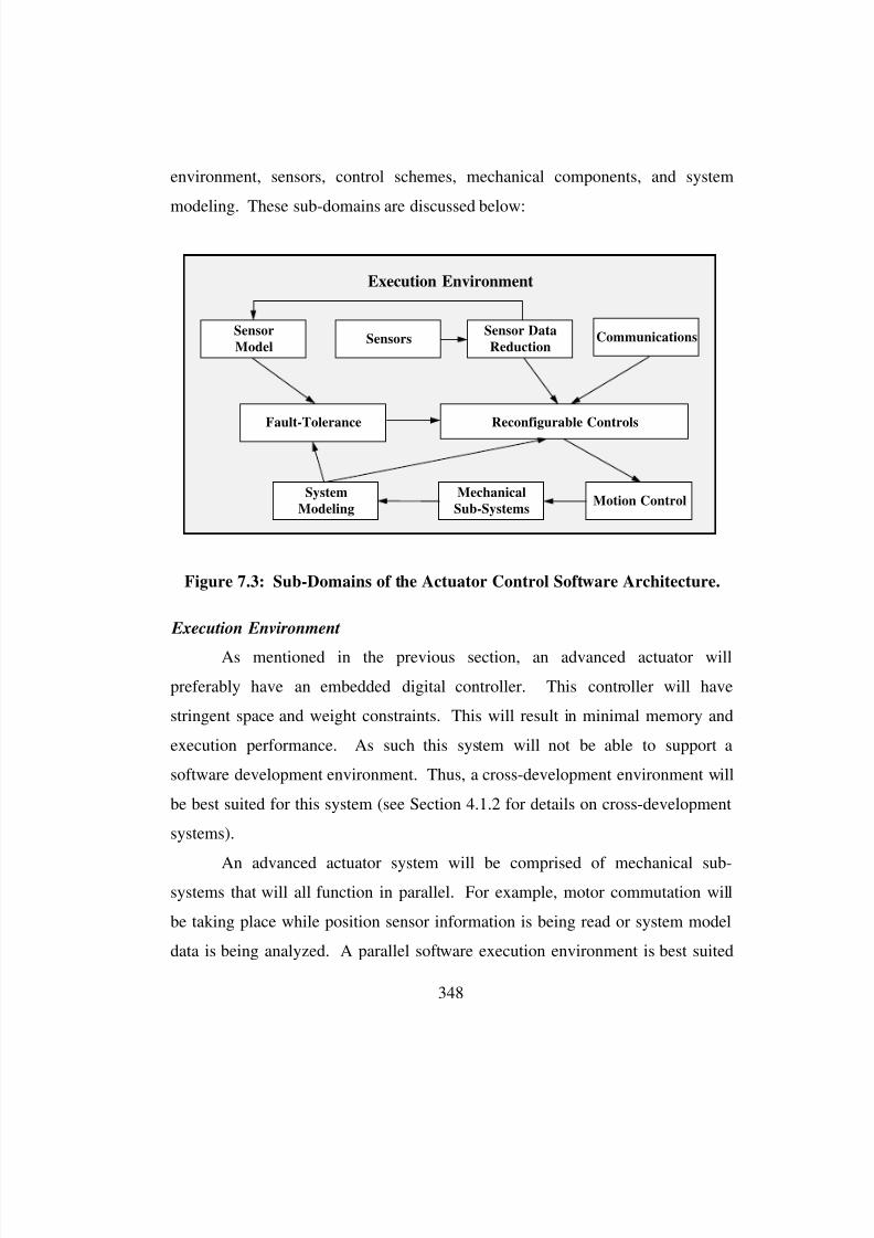
8/3/2019 Chetan Kapoor Dissertation
http://slidepdf.com/reader/full/chetan-kapoor-dissertation 372/612
348
environment, sensors, control schemes, mechanical components, and system
modeling. These sub-domains are discussed below:
Execution Environment
As mentioned in the previous section, an advanced actuator will
preferably have an embedded digital controller. This controller will have
stringent space and weight constraints. This will result in minimal memory and
execution performance. As such this system will not be able to support a
software development environment. Thus, a cross-development environment will
be best suited for this system (see Section 4.1.2 for details on cross-development
systems).
An advanced actuator system will be comprised of mechanical sub-systems that will all function in parallel. For example, motor commutation will
be taking place while position sensor information is being read or system model
data is being analyzed. A parallel software execution environment is best suited
Execution Environment
Sensor Data
ReductionSensors
Reconfigurable Controls
Motion ControlSystem
Modeling
Fault-Tolerance
Sensor
ModelCommunications
Mechanical
Sub-Systems
Figure 7.3: Sub-Domains of the Actuator Control Software Architecture.

8/3/2019 Chetan Kapoor Dissertation
http://slidepdf.com/reader/full/chetan-kapoor-dissertation 373/612
349
for such a hardware system. Most real-time operating systems support a parallel
execution environment.
An advanced actuator is proposed to have ten sensors. These sensors will
be read continuously. However, all the data generated from these sensors will not
be equally important. The computer resources of the actuator should be
prioritized based on the importance of a particular sensory input. This
prioritization should be reconfigurable in real-time. For example, an actuator
running a servo control loop at a rate of 2000 Hertz may require a dynamic
reconfiguration of system resources every 0.5 milliseconds. An example of the
need for dynamic reconfiguration occurs when the temperature sensor gives an
abnormal reading. At this point the priority of the system resource dedicated to
analyzing the data from the sound sensor should increase. This way, by fusing
the temperature data and the sound data a specific decision could be made about
an impending fault. The priority based allocation of resources is another
characteristics of real-time operating systems.
The data being generated inside an actuator will have to be handled in
real-time. For example, for an actuator with a 2000 Hertz servo-loop, externalevents will have to be handled within 0.5 milliseconds to maintain control
stability. Deterministic event handling is another characteristic of real-time
operating systems. Again, event handling should also be based on priority. Some
events would be more crucial for actuator operation than other events.
Communications
This domain will support software that will allow for communication with
the system controller. The communication domain will interpret the data received
from the system controller and pass it on to the reconfigurable control domain.
Device drivers for various communication protocols will be included in this
domain. This domain will also include components that will allow
communication between different sub-domains of the actuator control software.
8/3/2019 Chetan Kapoor Dissertation
http://slidepdf.com/reader/full/chetan-kapoor-dissertation 374/612
350
An example of this would be shared-memory and message passing. The
communication domain will rely heavily on the operating system constructs to
support various communication protocols.
Reconfigurable Controls
This domain will implement various control schemes. Examples of these
are PID, model-based, adaptive, optimal, etc. These control schemes will further
rely on input from the system modeling domain for performance maximization.
The fault-tolerance sub-domain will inform this domain regarding any changes to
the system configuration. The sensor data reduction sub-domain will present
sensory input in a consistent and simplified format to this domain. The output of
this domain will be sent to the motion control sub-system.
Motion Control
The motion control sub-system is responsible for generating current and
voltage commands that are sent to the motors. Algorithms for control of different
types of motors will be implemented here. For example, for a brushless dc motor,
various commutation schemes will have to be implemented. For stepper motors,
various stepping schemes, for example, micro-stepping will have to beimplemented. Additionally, the motion control sub-system will also implement
various motion profiling schemes. An example of this is the trapezoidal velocity
profile. The motion control sub-system will output its command to the
mechanical system. The mechanical system will include the motor, the brake,
and the clutch.
Sensors
Sensors will play a key role in the development of advanced actuators.
The multitude of sensors will lead to a confusing environment that would produce
more information than could be analyzed. This is where a well designed layered
software architecture could simplify things. The ten different sensor types were
discussed in the previous sections. A software architecture has to be designed

8/3/2019 Chetan Kapoor Dissertation
http://slidepdf.com/reader/full/chetan-kapoor-dissertation 375/612
351
that encompasses all different types of sensing, and also different types of sensors
for each sense type. For example, an abstract software component whose
interface reflects the functionality of position sensors could be created. This
component should define the interface for all possible position sensors. Derived
from this component should be specializations of a position sensor. Examples of
these would be encoder, potentiometer, etc. Similar abstract types will have to be
created for all other sensors. The advantage of this would be that the type of a
sensor may be swapped without changing the architecture and connectivity of the
remaining software. Components from this domain will be used by sensor data
reduction and for generating a sensor model of the system.
Sensor Data Reduction
The advanced actuator has ten different sensors. Ten different outputs
will be generated by these sensors. Not all of these outputs will be used at any
given instance. Different sensor outputs will be selected based on the control
scheme being used. Also, the output of two or more sensors may have to be
combined to construe a logical result. This is what is referred to as sensor data
reduction or sensor fusion. A software architecture and algorithms have to bedeveloped for logical sensor fusion and data reduction. The output of sensor data
reduction will be used by the reconfigurable controls to provide feedback into the
system. Also, using the reduced sensor data, a model of the system will be
generated. This will be referred to as the sensor model.
System Model
The purpose of this domain is the real-time computation of the system
model. This system model will be formulated using as-built parameters of the
robot. The system model will further draw on the mechanical sub-system models
to build a complete model. The software architecture for the system model
should be general enough to apply to a large variety of actuators.
Mechanical Components

8/3/2019 Chetan Kapoor Dissertation
http://slidepdf.com/reader/full/chetan-kapoor-dissertation 376/612
352
The mechanical components domain will contain software components
that emulate and interface to the mechanical hardware. For example, in this
domain there may be a software component called “Brake.” This component will
be a abstract component that defines the functionality of all types of brakes.
Additionally, this component will have functionality to access the parameters of a
brake. These parameters will be used by the system model sub-domain to create a
model reference. Thus, this domain will provide abstract components for all
mechanical sub-systems. Specific functionality for these sub-systems will be
added based on the particular type of sub-system used. For example, when a
particular brake is added to the actuator, a new software component that
encapsulates its functionality will be defined. This component will be derived
from the abstract brake component and it will inherit its interface and some of its
functionality.
Fault-Tolerance
A software architecture for the fault-tolerance domain will have to be
developed for actuators to be used in space. The purpose of this domain would be
to detect incipient faults, identify these faults, and take remedial action. Thefault-detection will take place by continuously comparing a sensor model of the
system to a mathematical model of the system. Discrepancies in the comparison
will be used to identify faults. This domain will also contain software
components for fault recovery. The fault-recovery component will inform the
reconfigurable control domain of the change in the system after a fault was
detected6.
7.4.3.2. Software Architecture for Manual Controller Integration
6 Dissertation on fault-tolerance in progress by Natalia Sharygina at the Robotics Research Group
8/3/2019 Chetan Kapoor Dissertation
http://slidepdf.com/reader/full/chetan-kapoor-dissertation 377/612
353
This research incorporated manual controller integration into the OSCAR
architecture. However, all the manual controllers that were used had software
specifically developed for each of them. There was little software reuse. Also,
each manual controller had its own interface. It is desired that a software
architecture be developed that incorporates all classes of manual controllers. This
architecture will include a set of abstract components that define the interface for
using all manual controllers.
There are two types of manual controllers. The first one is similar to a
joysticks and can be used only for open-loop control. The other one includes
force-reflection. The software architecture should define the interface for both
types of manual controllers. Once this interface is defined, new components can
be created that have the same interface but encapsulate functionality specific to
particular manual controllers. The work done by Peterson [1996] should be used
for detailed analysis of the domain and design of the software architecture7.
A preliminary class hierarchy for this architecture is shown in Figure 7.4.
In this class hierarchy the Manual Controller base class defines the interface for a
open-loop manual controller (the interface is italicized). From this class arederived the Keyboard and the TeachBall (see Section 4.6). Both the computer
keyboard and the TeachBall can be used to control robots in open-loop. The
Force Reflecting manual controller is derived from Manual Controller base class.
Here the interface for reflecting forces is added. From the Force Reflecting
controllers are derived the Robot Arm Type controllers and the PerForce
Controller. The PerForce Controller class adds specific functionality to deal with
the Cybernetics PerForce controller (see Section 4.6). The Robot Arm Type
controller will use OSCAR for computing the forward kinematics solution and the
7 Masters thesis on dual-force sensing for manual controllers in progress by Robert Hester at the
Robotics Research Group
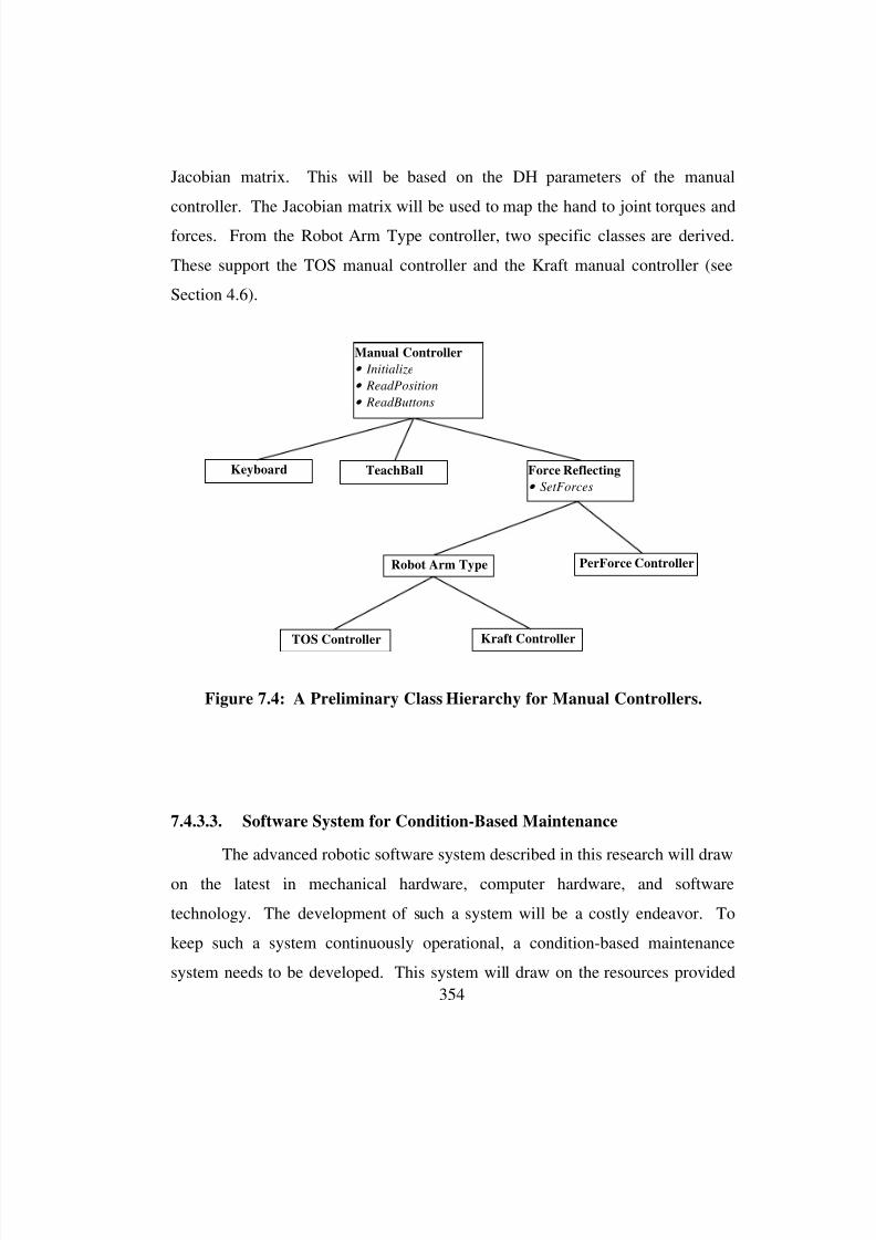
8/3/2019 Chetan Kapoor Dissertation
http://slidepdf.com/reader/full/chetan-kapoor-dissertation 378/612
354
Jacobian matrix. This will be based on the DH parameters of the manual
controller. The Jacobian matrix will be used to map the hand to joint torques and
forces. From the Robot Arm Type controller, two specific classes are derived.
These support the TOS manual controller and the Kraft manual controller (see
Section 4.6).
7.4.3.3. Software System for Condition-Based Maintenance
The advanced robotic software system described in this research will draw
on the latest in mechanical hardware, computer hardware, and software
technology. The development of such a system will be a costly endeavor. To
keep such a system continuously operational, a condition-based maintenance
system needs to be developed. This system will draw on the resources provided
Manual Controller
• Initialize
• ReadPosition
• ReadButtons
Force Reflecting
• SetForces
Robot Arm Type
TeachBallKeyboard
TOS Controller Kraft Controller
PerForce Controller
Figure 7.4: A Preliminary Class Hierarchy for Manual Controllers.

8/3/2019 Chetan Kapoor Dissertation
http://slidepdf.com/reader/full/chetan-kapoor-dissertation 379/612
355
by OSCAR and the real-time control layer to produce a time-sheet for
maintenance.
The condition-based system will consist of a high-speed archiver (a
database) that will be used to store operational history of a system. The
condition-based maintenance system will continuously (once very five seconds)
monitor the sensory input coming in from the real-time control layer. It will also
gather the mathematically modeled state of the system from OSCAR. Both the
mathematical model information and sensor information will be archived and also
analyzed for discrepancies. Discrepancies in the sensor information and the
model information will warn about an impending failure. An empirical analysis
of the archived data will be used to determine detailed information about the
impending fault. The advantage of archiving data is that the more a machine is
used, the better understood will be its behavior.
7.4.4. Agile Manufacturing of Software
Any mature industry is characterized by a component industry. However,
for effective use of available components, it is important to have a process in
place for component selection and component assembly [Yeh, 1993]. This has to
be achieved for robotic software also. OSCAR provides some of the components
for robot control. However, the component selection is currently left to the
applications developer. The assembly of these components is also done by the
applications developer. To automate the component selection and assembly
process, future work needs to be done in the following areas:
• Component selection system.
• Component assembly system.

8/3/2019 Chetan Kapoor Dissertation
http://slidepdf.com/reader/full/chetan-kapoor-dissertation 380/612
356
The software components combined with the component selection process
and assembly process will offer an environment for agile manufacturing of
software for system controllers. This concept is illustrated in Figure 7.5. The
input into this system are the application requirements. The application
requirements are generated from application components. For example, a high-
speed assembly operation that also has a force-fit task will comprise of two
components. These will be ‘high-speed’ and ‘force-fit.’ Based on the application
components, an optimized application process will be designed. At this point
there is refinement and testing of this process. The specifications of the
application process are then passed to the component selection and componentassembly systems. These systems are explained below:
7.4.4.1. Component Selection System
Application
Components
SCAD
Man-machine Interface
Components
Operational Software
Components
Real-time ControlComponents
Application
Process
(re)design
Software
Development/
Integration/
Assembly
Integrated
Target
Application
Prototyping/
Refinement
Prototyping/ Refinement/
Testing
Figure 7.5: An Agile Software Manufacturing Framework for System
Control Software.

8/3/2019 Chetan Kapoor Dissertation
http://slidepdf.com/reader/full/chetan-kapoor-dissertation 381/612
357
The information generated by the application process design is passed to
the software components selection sub-system (SCAD). SCAD stands for
software CAD and it allows the optimal selection of software modules from the
three layers of system control software. Internal to SCAD, refinement and testing
of the selected software modules takes place. This testing should not be confused
with the unit testing of the components. Unit testing of the components had to be
accomplished after component design. The testing taking place inside SCAD
validates the suitability of a component for the application process (For details on
how SCAD fits into the complete robotic system design tool see Section 2.1).
7.4.4.2. Component Assembly System
The next step after selection of components by SCAD is their assembly.
The assembly of these components will depend on the selected components and
the application process. Currently, this is done manually by the program
developer. In the future this system should include an automatic code generator.
This generator should be able to create a code framework into which the selected
components will fit. The generated code will then be tested and finally a target
application will be created.
Commercially, there are systems available that assist in component
assembly. Most of these systems are used in visual programming environment
such as LabView [National Instruments, 1996] and Microsoft Visual C++.
However, these systems are not intelligent enough to assist in component
selection. The user has to specify the components to use and usually has to
connect them together (visually). Research at Carnegie Mellon University has led
to the design of a similar system (as shown in Figure 7.5) for computer design
[Birmingham and Gupta, 1988]. This system (called MICON) is an integrated
collection of programs that automatically synthesize small computer systems
from high-level specifications. MICON is based on a knowledge based synthesis
8/3/2019 Chetan Kapoor Dissertation
http://slidepdf.com/reader/full/chetan-kapoor-dissertation 382/612
358
tool and an automated knowledge acquisition tool. A database and a data
management tool are integrated into this system.
7.4.5. Software Organization and Management Process
The lessons acquired during the course of this research pointed out the
importance of software organization and management of the development
process. For this purpose, software development guidelines were put in place for
the Robotics Research Group (see Appendix A). However, this was the first
attempt at major software development. The needs at the Robotics Research
Group will change as the size of the software increases and more developers start
using OSCAR. The complexity of managing this process will also increase as
more hardware platforms and operating systems will be supported. The software
development guidelines will have to be continually updated and enhanced.
Currently, the software development is managed by makefiles [Oram, and
Talbott, 1995]. Source code control is useful for maintaining older versions,
documenting changes, and allowing multiple developers to work with the same
source code [Bolinger and Bronson, 1995]. A preliminary application of source
code is already in place. However, a complete application of this needs to be
done. Further, the makefiles have to be enhanced to support software
development for Windows NT. Currently, the makefile support development for
VxWorks and Solaris operating systems. For this to be possible, Windows NT
PC and the SUN Workstation will have to share source code.
7.4.6. Manufacturing Cell Development
The culmination of this research and the proposed future work will be a
meaningful application. Manufacturing cells provide an ideal environment for
this application. Manufacturing cells bring us a step closer to achieving the goals
of agile manufacturing. Agile manufacturing focuses on fulfilling orders,
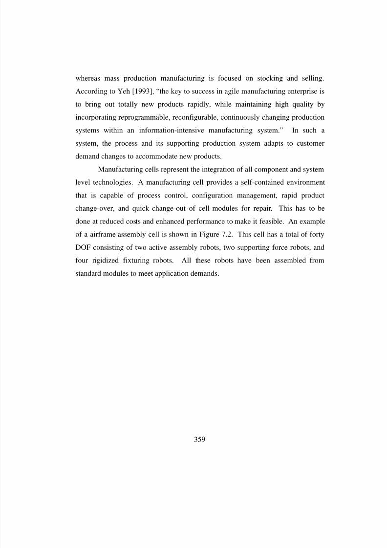
8/3/2019 Chetan Kapoor Dissertation
http://slidepdf.com/reader/full/chetan-kapoor-dissertation 383/612
359
whereas mass production manufacturing is focused on stocking and selling.
According to Yeh [1993], “the key to success in agile manufacturing enterprise is
to bring out totally new products rapidly, while maintaining high quality by
incorporating reprogrammable, reconfigurable, continuously changing production
systems within an information-intensive manufacturing system.” In such a
system, the process and its supporting production system adapts to customer
demand changes to accommodate new products.
Manufacturing cells represent the integration of all component and system
level technologies. A manufacturing cell provides a self-contained environment
that is capable of process control, configuration management, rapid product
change-over, and quick change-out of cell modules for repair. This has to be
done at reduced costs and enhanced performance to make it feasible. An example
of a airframe assembly cell is shown in Figure 7.2. This cell has a total of forty
DOF consisting of two active assembly robots, two supporting force robots, and
four rigidized fixturing robots. All these robots have been assembled from
standard modules to meet application demands.
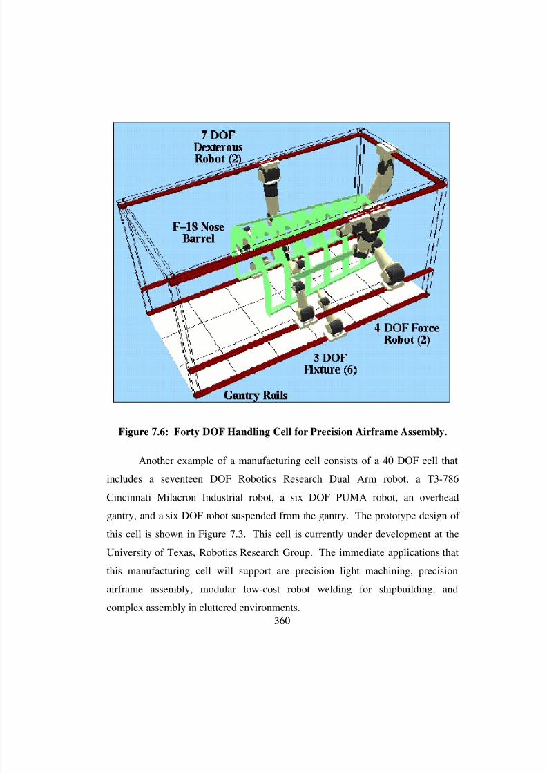
8/3/2019 Chetan Kapoor Dissertation
http://slidepdf.com/reader/full/chetan-kapoor-dissertation 384/612
360
Another example of a manufacturing cell consists of a 40 DOF cell that
includes a seventeen DOF Robotics Research Dual Arm robot, a T3-786
Cincinnati Milacron Industrial robot, a six DOF PUMA robot, an overhead
gantry, and a six DOF robot suspended from the gantry. The prototype design of
this cell is shown in Figure 7.3. This cell is currently under development at the
University of Texas, Robotics Research Group. The immediate applications that
this manufacturing cell will support are precision light machining, precision
airframe assembly, modular low-cost robot welding for shipbuilding, and
complex assembly in cluttered environments.
Figure 7.6: Forty DOF Handling Cell for Precision Airframe Assembly.
8/3/2019 Chetan Kapoor Dissertation
http://slidepdf.com/reader/full/chetan-kapoor-dissertation 385/612
361
A manufacturing cell can serve different types of applications. Based on
the application, manufacturing cells will draw on all aspects of OSCAR and the
proposed future work. For example, precision applications will use a precisely
calibrated robot. This robot will require an inverse kinematics method general
with respect to geometry. Also, as manufacturing cells will support
reconfigurability, the software should be general to support all possible
configurations. Complex assembly tasks will require that the robot operate in a
cluttered environment. This will involve the robot reaching into a “tight” space or
Figure 7.7: A Prototype Forty DOF Manufacturing Cell.
8/3/2019 Chetan Kapoor Dissertation
http://slidepdf.com/reader/full/chetan-kapoor-dissertation 386/612
362
reach around an intermediate object. A redundant arm will be needed in this
application. The software should be able to support the kinematics of this arm.
Moreover the kinematics should support obstacle avoidance.
7.4.6.1. Influence of This Research on Manufacturing Cell Development
This research was based on developing software components that could be
used by a software selection system that was based on task requirements. This
concept was a part of an Interactive Synthesis Tool for Advanced Robotics (I-
STAR) (see Section 2.1). I-STAR was further comprised of a three major sub-
systems. These were a mechanical module selection system (MCAD), a software
module selection system (SCAD), and a controller module selection system
(CCAD). In the original concept of I-STAR, MCAD, SCAD, and CCAD were
equally important. This research has however tilted the balance towards SCAD.
The primary reasons for SCAD becoming a more complex system that requires
substantial development efforts are:
• System controller technology will achieve standardization and will become
available as a collection of low-cost personal computers that can be assembled
on demand. Also, the granularity of the assembled systems will be somewhat
higher. For example, earlier systems were based on tight-coupling of multiple
processors. This might change to a distributed computing environment that is
comprised of multiple personal computers that are connected using high-
speed communication links. Due to these changes, the importance of CCAD
has considerably decreased.
• The actuator (or mechanical components) will be much more complex than
perceived in I-STAR. However, there will be fewer different types of
actuators but will be much more standardized (both in their interfaces and in
their models). As a consequence, the collection of standard modules
necessary to create a very large population of systems will go down

8/3/2019 Chetan Kapoor Dissertation
http://slidepdf.com/reader/full/chetan-kapoor-dissertation 387/612
363
considerably8. Hence, the emphasis in I-STAR for their selection is
diminished.
• What has happened, however, is that the complexity and required generality
of object-oriented software (therefore OSCAR and its future generations) has
expanded dramatically. For example, a single mechanical module (an
actuator) may now need more than 30 different software modules to fully
extract its functionality. This will lead to an increase in the importance of the
SCAD selection process that was envisioned in I-STAR. This is significant
for manufacturing cell development. Software modules are now required to
adhere to strict standards and should exhibit reuse via generality and
extensibility. This research is a step towards this goal.
7.4.6.2. Desired Software Functionality for Cell Operation
The development of manufacturing cell technology is the ultimate goal of
the Robotics Research Group. This research has led to the development of
software components that will be instrumental in the development of a
manufacturing cell. However, not all software areas that are required for
manufacturing cell development have been addressed. These are listed in Table
7.13. It should be noted that some of the issues listed in Table 7.13 were
addressed by OSCAR. The issues that were not addressed will also draw upon
the functionality provided by OSCAR.
8 A result of extensive discussions with D. Tesar in August of 1996.
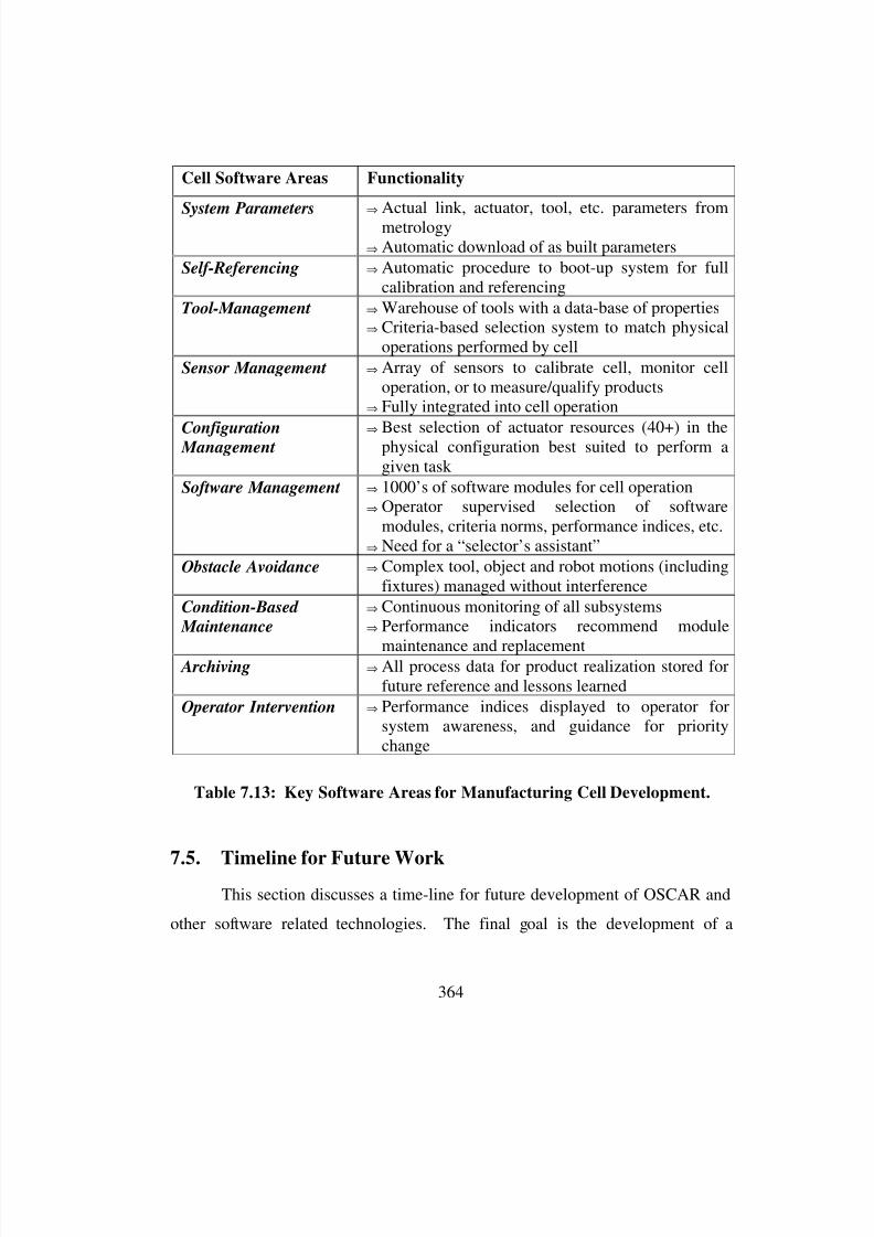
8/3/2019 Chetan Kapoor Dissertation
http://slidepdf.com/reader/full/chetan-kapoor-dissertation 388/612
364
7.5. Timeline for Future WorkThis section discusses a time-line for future development of OSCAR and
other software related technologies. The final goal is the development of a
Cell Software Areas Functionality
System Parameters⇒
Actual link, actuator, tool, etc. parameters frommetrology⇒ Automatic download of as built parameters
Self-Referencing ⇒ Automatic procedure to boot-up system for fullcalibration and referencing
Tool-Management ⇒ Warehouse of tools with a data-base of properties⇒ Criteria-based selection system to match physical
operations performed by cell
Sensor Management ⇒ Array of sensors to calibrate cell, monitor celloperation, or to measure/qualify products
⇒ Fully integrated into cell operation
Configuration Management⇒
Best selection of actuator resources (40+) in thephysical configuration best suited to perform agiven task
Software Management ⇒ 1000’s of software modules for cell operation⇒ Operator supervised selection of software
modules, criteria norms, performance indices, etc.⇒ Need for a “selector’s assistant”
Obstacle Avoidance ⇒ Complex tool, object and robot motions (includingfixtures) managed without interference
Condition-Based Maintenance
⇒ Continuous monitoring of all subsystems⇒ Performance indicators recommend module
maintenance and replacement Archiving ⇒ All process data for product realization stored for
future reference and lessons learned
Operator Intervention ⇒ Performance indices displayed to operator forsystem awareness, and guidance for prioritychange
Table 7.13: Key Software Areas for Manufacturing Cell Development.
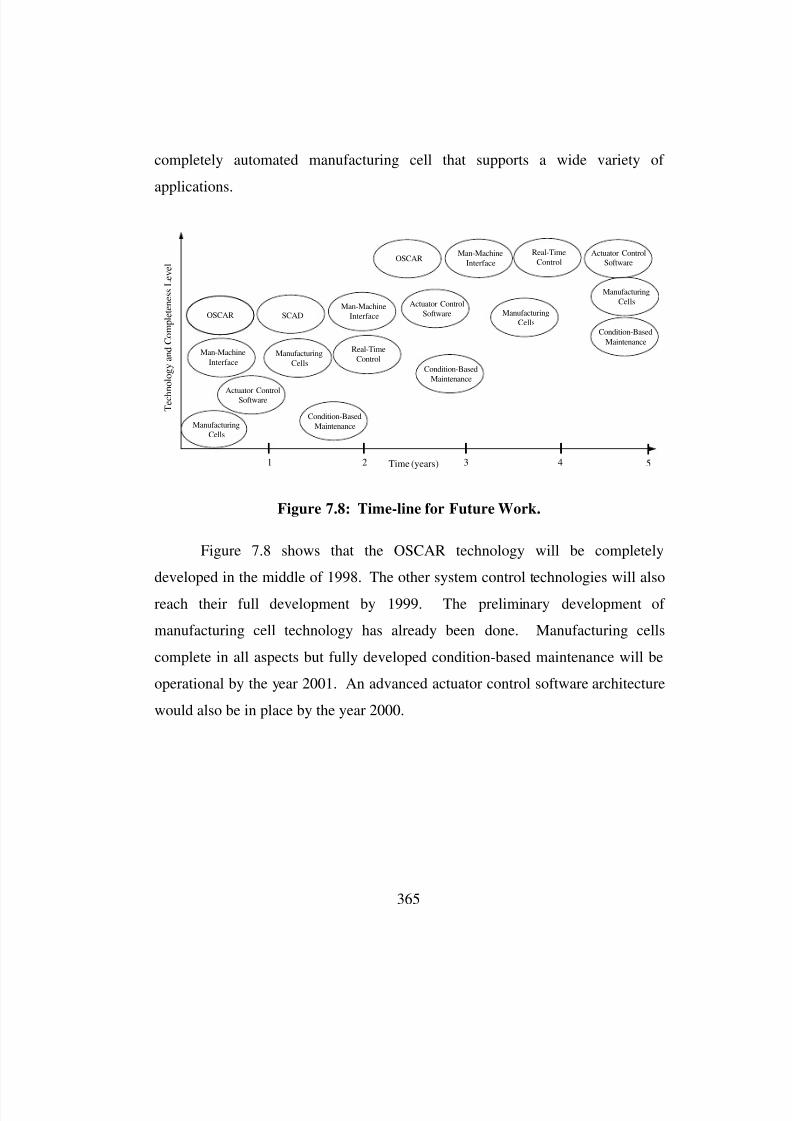
8/3/2019 Chetan Kapoor Dissertation
http://slidepdf.com/reader/full/chetan-kapoor-dissertation 389/612
365
completely automated manufacturing cell that supports a wide variety of
applications.
Figure 7.8 shows that the OSCAR technology will be completely
developed in the middle of 1998. The other system control technologies will also
reach their full development by 1999. The preliminary development of
manufacturing cell technology has already been done. Manufacturing cells
complete in all aspects but fully developed condition-based maintenance will be
operational by the year 2001. An advanced actuator control software architecture
would also be in place by the year 2000.
T e c h n o l o g y a n d C o m p l e t e n e s s L e v e l
Time (years)
OSCAR SCAD
Real-TimeControl
Man-Machine
Interface
Man-MachineInterface
Actuator ControlSoftware
Actuator ControlSoftware
ManufacturingCells
1 2 3 4 5
Man-MachineInterface
ManufacturingCells
ManufacturingCells
ManufacturingCells
Condition-BasedMaintenance
Condition-BasedMaintenance
Condition-Based
Maintenance
OSCARReal-Time
ControlActuator Control
Software
Figure 7.8: Time-line for Future Work.
8/3/2019 Chetan Kapoor Dissertation
http://slidepdf.com/reader/full/chetan-kapoor-dissertation 390/612
369
Appendix A
A. Software Development Guidelines
This document proposes a software design and development philosophy
for current and future software development at the Robotics Research Group.
First the design philosophy is discussed. Then a synopsis of the design process is
given. After that, some programming guidelines are stated and some sample code
is listed.
A.1. Software Design Philosophy
All mature industries, like the automobile industry, are characterized by
the presence of a component’s industry. For example, an automobile is made up
of components that are supplied from different vendors. Currently there is a
revolution taking place in the commercial software industry. This has been
brought on by the popularity of object-oriented design. A similar revolution is
desired in the intelligent machine's software industry. This can be achieved by
stressing the development of software modules (henceforth called components)
which have the following characteristics:• Standardized Interfaces,
• Completeness and abstractness (should have a black box appearance),
• Reusability, and
8/3/2019 Chetan Kapoor Dissertation
http://slidepdf.com/reader/full/chetan-kapoor-dissertation 391/612
370
• Portability.
For a long time, software development was directed towards fulfillingproject goals. This often led to the development of shoddy software that had little
reuse potential. This made future releases harder and more expensive. Emerging
software design philosophies stress the development of robust components that
can be modified and assembled to achieve project goals. Keeping this paradigm
shift in mind, the software design philosophy of the Robotics Research Group can
be summed up in one line:
“From Projects to Components.”
A.2. How do we achieve our design goals?
One means of achieving our design goal of building reusable components
is to develop software using object-oriented programming. Object-oriented
programming has four key components. These are:
• Information hiding,
• Data abstraction,
• Dynamic binding, and
• Inheritance.
Classes, a key component of object-oriented programming (in C++)
provide all the information necessary to construct and use objects of a particular
type. A class here is analogues to a template from which instances (objects) can
be created. Each instance has a state associated with it.
Information hiding is achieved by hiding the inner working details of a
class. This helps in avoiding inter-dependencies between components and also
makes modification easier.
8/3/2019 Chetan Kapoor Dissertation
http://slidepdf.com/reader/full/chetan-kapoor-dissertation 392/612
371
Data-abstraction is used to abstract the functionality of a class and give it a
black-box look and feel.
Dynamic binding is used for dynamic polymorphism and to avoid the use
of switch statements to determine the type of an object (e.g., which class was it
instantiated from).
Inheritance provides us a means of sub-classing. It allows for creation of
new classes by specifying the differences between the new class and an existing
class. This promotes reusability (see section 2.5 for details on software design).
Another issue to consider in the design and specification of components is
the types of reuse desired from the components. Components can offer reuse in
two forms: generality and extensibility. An example of generality are the first
generation of Macintosh computers. These Macintoshes were general enough to
run different software but were not extensible. That is, you could not make
hardware modifications like adding RAM. Our goal is to exploit reuse through
generality and extensibility. To achieve this kind of reuse, a solid set of
methods and techniques is desired.
A.3. The Design Process
This section gives a brief outline of traditional engineering software
design and object-oriented software design as specified by Booch [1994]. This
information is compiled from books on engineering design and software design.
An interesting thing to note is that none of the software design books reference
the work done in the area of engineering design in the earlier part of this century.
This is perplexing, as these books contain a wealth of design information that is
applicable to all systems.
8/3/2019 Chetan Kapoor Dissertation
http://slidepdf.com/reader/full/chetan-kapoor-dissertation 393/612
372
A.4. Traditional Engineering Design
A.4.1. What is Design?
As defined by Pahl and Beitz [1988], “Designing is an intellectual attempt
to meet demands in the best possible way. A systematic design alone can produce
rational solutions.”
A.4.2. What are the qualities of a good designer?
• Initiative,
• Resolution,
• Economic Insight,
• Tenacity,
• Optimism,
• Sociability, and
• Teamwork.
A.4.3. Summary of the Design Process
1. Task clarification,
2. Conceptual design,
3. Embodiment design, and
a) Layout design
b) Form design
4. Detail design.
All throughout the design process one should have:⇒ the required motivation,
⇒ clarify the boundary conditions,
⇒ dispel prejudice,
8/3/2019 Chetan Kapoor Dissertation
http://slidepdf.com/reader/full/chetan-kapoor-dissertation 394/612
373
⇒ look for variants,
⇒
make decisions, and⇒ balance between an intuitive approach and a systematic approach.
A.4.4. Critical Path Analysis
A critical path analysis allows designers to manage time for
⇒ feasibility study,
⇒ search for solutions, and
⇒ evaluation of results.
A.5. Software Design Process
There are three steps in object-oriented software development as specified
by Booch [1994] [White]. These are outlined in the following sections:
A.5.1. Requirement Analysis
The objectives of requirements analysis are:
• To find out what customers want the system to do, and
• to form a contract between the customer and the developer.
The deliverables of the requirement analysis are:
• System Charter: This outlines the responsibilities of the system.
• System Function Statement: This outlines the key use cases of the system.
A.5.2. Domain Analysis
The objectives of domain analysis are:• Add appropriate level of abstraction to a system.
• Identify all major objects in the domain including all data and major
operations.
8/3/2019 Chetan Kapoor Dissertation
http://slidepdf.com/reader/full/chetan-kapoor-dissertation 395/612
374
The deliverables of domain analysis are:
•
Class diagrams that identify the key classes, or types, of the domain.• Class specification, which contain all semantic definitions of the classes, their
relationships, their attributes, and their key operations.
• Object-scenario diagrams, which illustrate how the objects will interact to
carry out key system functions.
• Data dictionary, which lists all domain entities including classes,
relationships, and attributes.
The steps involved in domain analysis are:
• define Classes,
• define relationships,
• define operations,
• find attributes (properties that describe that class),
• define inheritance, and
• validate and iterate.
A.5.3. System Design
The objectives of system design are:
• Determine effective, efficient, and cost-effective implementation to carry out
the function.
• To map ideal or logical analysis developed during domain analysis to objects
and classes that can be coded.
The deliverables of system design are:
• Architectural description, that is, hardware, CPU, OS, language, etc.
• Executable release descriptions.
8/3/2019 Chetan Kapoor Dissertation
http://slidepdf.com/reader/full/chetan-kapoor-dissertation 396/612
375
• Class-category diagrams, which model the partitioning of the system into
high-level groups.• Design class diagrams, which show detail data types and structures, etc.
• Design object-scenario diagrams, which show detail operational logic.
• New specifications supporting these diagrams.
• Amended class specifications showing full operational specifications for those
operations with complex algorithms (very valid in robotic software).
The steps involved in system design are:
•
determine initial architecture,• plan executable releases,
• develop executable releases,
• refine the design.
This section gave a brief overview of the iterative process of object-
oriented analysis and design. As a class is a key component of object-oriented
software, meaningful names should be used for them. Ill defined names simply
imply ill-defined abstractions. Also, a good class has loose or weak coupling and
does not have many relationships to other classes outside its supertypes or
subtypes. For more details on the process of object-oriented software design refer
to Booch [1994].
A.6. Programming Guidelines
1. The programming guidelines outlined here fall into three general categories.
These author was exposed to these guidelines while working at National
Instruments. The details of these guidelines are listed in Kapoor [1995] and
an example application of these guidelines is given in the next section.

8/3/2019 Chetan Kapoor Dissertation
http://slidepdf.com/reader/full/chetan-kapoor-dissertation 397/612
376
A.7. Example
A.7.1. File Vector.hpp
////////////////////////////////////////////////////////////////////////////////////////////////////////////////////////////////////////// // // Title : Vector.hpp // Project : D&D // Created : 09/19/95 @ 23:35:30 Central Standard Time // Author : Chetan Kapoor // Platforms : All // Copyright : The University of Texas at Austin 1995. All Rights Reserved. // Access : Company Confidential // Purpose : This file implements the class declaration for an RRVector class
//-------------------------------------------------------------------------------------------------------------------------- // // Classes: // RRVector // // Global Functions: // <none> // // Global Variables: // <none> // //-------------------------------------------------------------------------------------------------------------------------- // // $Revision$ 1.0 // // $Log$ // New file created (19th September, 95) ///////////////////////////////////////////////////////////////////////////////////////////////////////////////////////////////////////////// #if !defined(Vector_hpp)#define Vector_hpp
//+====================================================================== // Includes //=======================================================================
#include <RRCommon.hpp>
#include <iostream.h>
//====================================================================== // Class declaration for RRVector begins //=======================================================================
class RRVector{
public:RRVector(unsigned int, double* elements = 0);
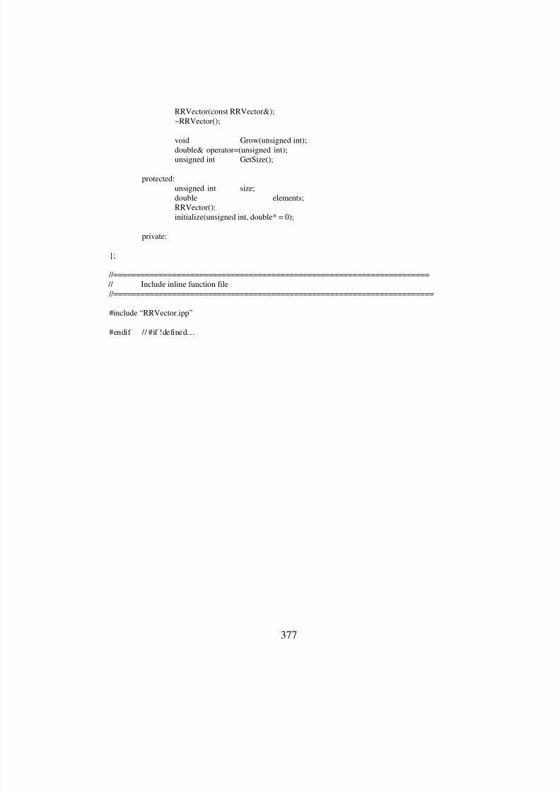
8/3/2019 Chetan Kapoor Dissertation
http://slidepdf.com/reader/full/chetan-kapoor-dissertation 398/612
377
RRVector(const RRVector&);~RRVector();
void Grow(unsigned int);double& operator=(unsigned int);unsigned int GetSize();
protected:unsigned int size;double elements;RRVector();initialize(unsigned int, double* = 0);
private:
};
//====================================================================== // Include inline function file //=======================================================================
#include “RRVector.ipp”
#endif // #if !defined....
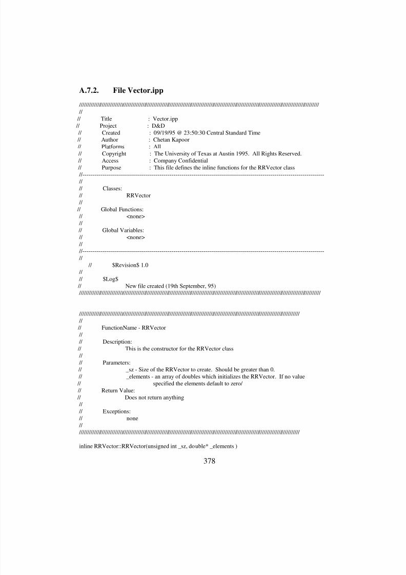
8/3/2019 Chetan Kapoor Dissertation
http://slidepdf.com/reader/full/chetan-kapoor-dissertation 399/612
378
A.7.2. File Vector.ipp
//////////////////////////////////////////////////////////////////////////////////////////////////////////////////////////////////////////////////// // // Title : Vector.ipp // Project : D&D // Created : 09/19/95 @ 23:50:30 Central Standard Time // Author : Chetan Kapoor // Platforms : All // Copyright : The University of Texas at Austin 1995. All Rights Reserved. // Access : Company Confidential // Purpose : This file defines the inline functions for the RRVector class //-------------------------------------------------------------------------------------------------------------------------- // // Classes: // RRVector
// // Global Functions: // <none> // // Global Variables: // <none> // //-------------------------------------------------------------------------------------------------------------------------- // // $Revision$ 1.0 // // $Log$ // New file created (19th September, 95) /////////////////////////////////////////////////////////////////////////////////////////////////////////////////////////////////////////////////////
//////////////////////////////////////////////////////////////////////////////////////////////////////////////////////////////////////// // // FunctionName - RRVector // // Description: // This is the constructor for the RRVector class // // Parameters: // _sz - Size of the RRVector to create. Should be greater than 0. // _elements - an array of doubles which initializes the RRVector. If no value // specified the elements default to zero/ // Return Value: // Does not return anything
// // Exceptions: // none // ////////////////////////////////////////////////////////////////////////////////////////////////////////////////////////////////////////
inline RRVector::RRVector(unsigned int _sz, double* _elements )

8/3/2019 Chetan Kapoor Dissertation
http://slidepdf.com/reader/full/chetan-kapoor-dissertation 400/612
379
{initialize(_sz, _elements);
}
//////////////////////////////////////////////////////////////////////////////////////////////////////////////////////////////////////// // // FunctionName - RRVector // // Description: // This is the const reference constructor (or copy constructor)for // the RRVector class // // Parameters: // _rrv - An RRVector from which the new RRVector is created // // Return Value: // Does not return anything
// // Exceptions: // none // ////////////////////////////////////////////////////////////////////////////////////////////////////////////////////////////////////////
inline RRVector::RRVector(const RRVector& _rrv){
initialize(_rrv.size, _rrv.elements);}
//////////////////////////////////////////////////////////////////////////////////////////////////////////////////////////////////////// // // FunctionName - RRVector //
// Description: // This is a protected constructor which is used by derived classes to bypass the // the use of the public constructors of this class. This constructor does nothing // but set elements = 0; // // Parameters: // none // // Return Value: // Does not return anything // // Exceptions: // none //
////////////////////////////////////////////////////////////////////////////////////////////////////////////////////////////////////////
inline RRVector::RRVector(){
elements = 0;}
////////////////////////////////////////////////////////////////////////////////////////////////////////////////////////////////////////
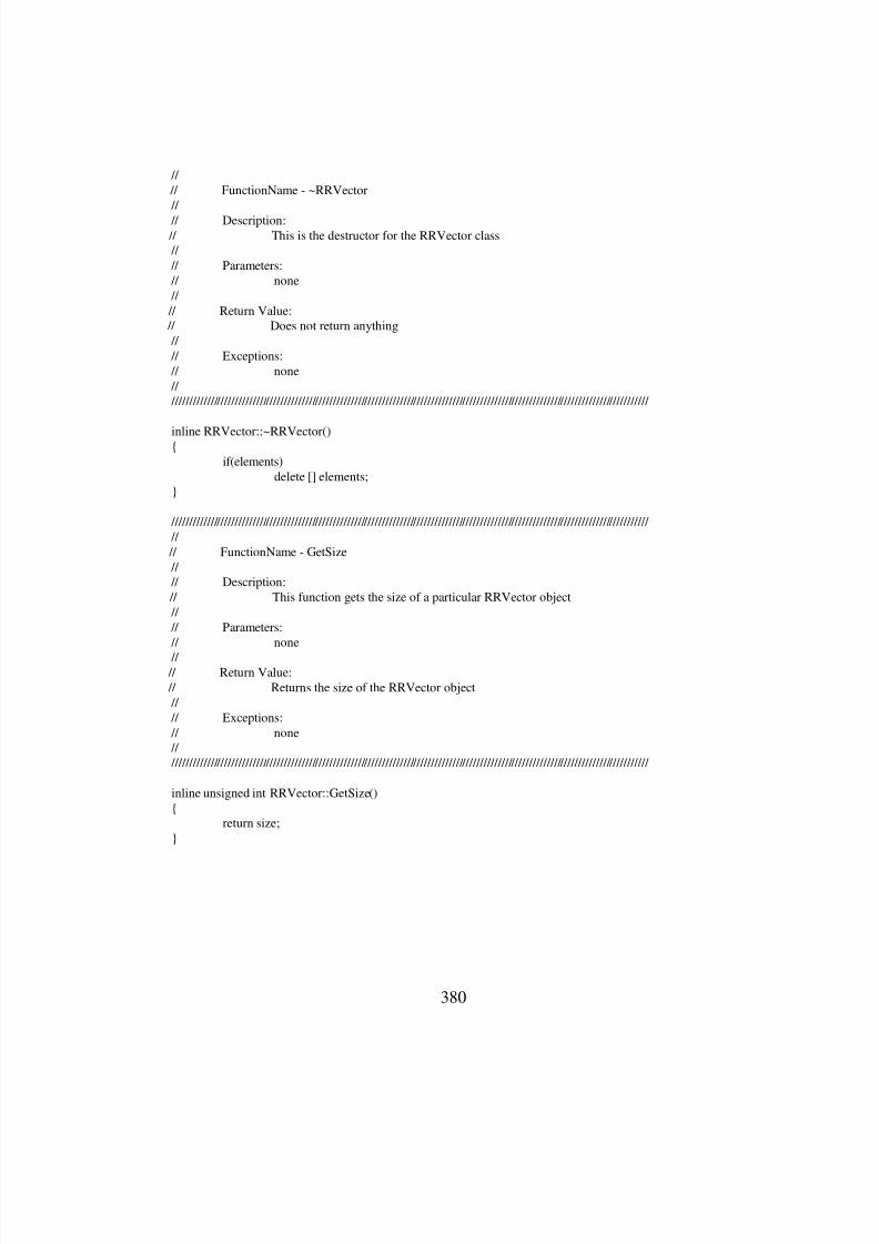
8/3/2019 Chetan Kapoor Dissertation
http://slidepdf.com/reader/full/chetan-kapoor-dissertation 401/612
380
// // FunctionName - ~RRVector //
// Description: // This is the destructor for the RRVector class // // Parameters: // none // // Return Value: // Does not return anything // // Exceptions: // none // ////////////////////////////////////////////////////////////////////////////////////////////////////////////////////////////////////////
inline RRVector::~RRVector(){if(elements)
delete [] elements;}
//////////////////////////////////////////////////////////////////////////////////////////////////////////////////////////////////////// // // FunctionName - GetSize // // Description: // This function gets the size of a particular RRVector object // // Parameters: // none
// // Return Value: // Returns the size of the RRVector object // // Exceptions: // none // ////////////////////////////////////////////////////////////////////////////////////////////////////////////////////////////////////////
inline unsigned int RRVector::GetSize(){
return size;}
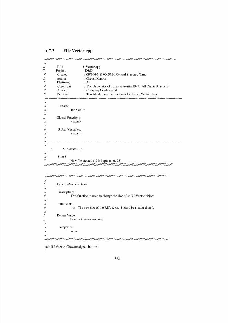
8/3/2019 Chetan Kapoor Dissertation
http://slidepdf.com/reader/full/chetan-kapoor-dissertation 402/612
381
A.7.3. File Vector.cpp
///////////////////////////////////////////////////////////////////////////////////////////////////////////////////////////////////////////////// // // Title : Vector.cpp // Project : D&D // Created : 09/19/95 @ 00:20:30 Central Standard Time // Author : Chetan Kapoor // Platforms : All // Copyright : The University of Texas at Austin 1995. All Rights Reserved. // Access : Company Confidential // Purpose : This file defines the functions for the RRVector class //-------------------------------------------------------------------------------------------------------------------------- // // Classes: // RRVector
// // Global Functions: // <none> // // Global Variables: // <none> // //-------------------------------------------------------------------------------------------------------------------------- // // $Revision$ 1.0 // // $Log$ // New file created (19th September, 95) /////////////////////////////////////////////////////////////////////////////////////////////////////////////////////////////////////////////
//////////////////////////////////////////////////////////////////////////////////////////////////////////////////////////////////////// // // FunctionName - Grow // // Description: // This function is used to change the size of an RRVector object // // Parameters: // _sz - The new size of the RRVector. S hould be greater than 0. // // Return Value: // Does not return anything //
// Exceptions: // none // ////////////////////////////////////////////////////////////////////////////////////////////////////////////////////////////////////////
void RRVector::Grow(unsigned int _sz ){
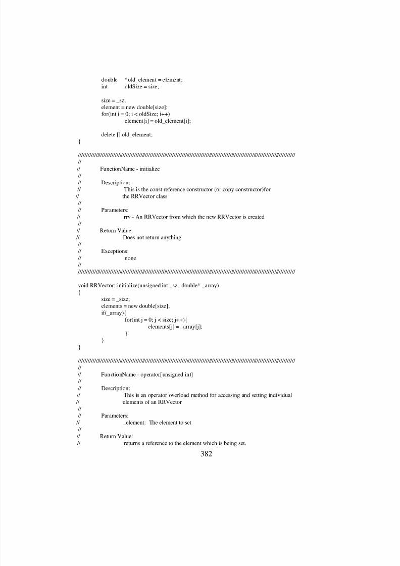
8/3/2019 Chetan Kapoor Dissertation
http://slidepdf.com/reader/full/chetan-kapoor-dissertation 403/612
382
double *old_element = element;int oldSize = size;
size = _sz;element = new double[size];for(int i = 0; i < oldSize; i++)
element[i] = old_element[i];
delete [] old_element;}
//////////////////////////////////////////////////////////////////////////////////////////////////////////////////////////////////////// // // FunctionName - initialize // // Description: // This is the const reference constructor (or copy constructor)for
// the RRVector class // // Parameters: // rrv - An RRVector from which the new RRVector is created // // Return Value: // Does not return anything // // Exceptions: // none // ////////////////////////////////////////////////////////////////////////////////////////////////////////////////////////////////////////
void RRVector::initialize(unsigned int _sz, double* _array){
size = _size;elements = new double[size];if(_array){
for(int j = 0; j < size; j++){elements[j] = _array[j];
}}
}
//////////////////////////////////////////////////////////////////////////////////////////////////////////////////////////////////////// // // FunctionName - operator[unsigned int] // // Description:
// This is an operator overload method for accessing and setting individual // elements of an RRVector // // Parameters: // _element: The element to set // // Return Value: // returns a reference to the element which is being set.
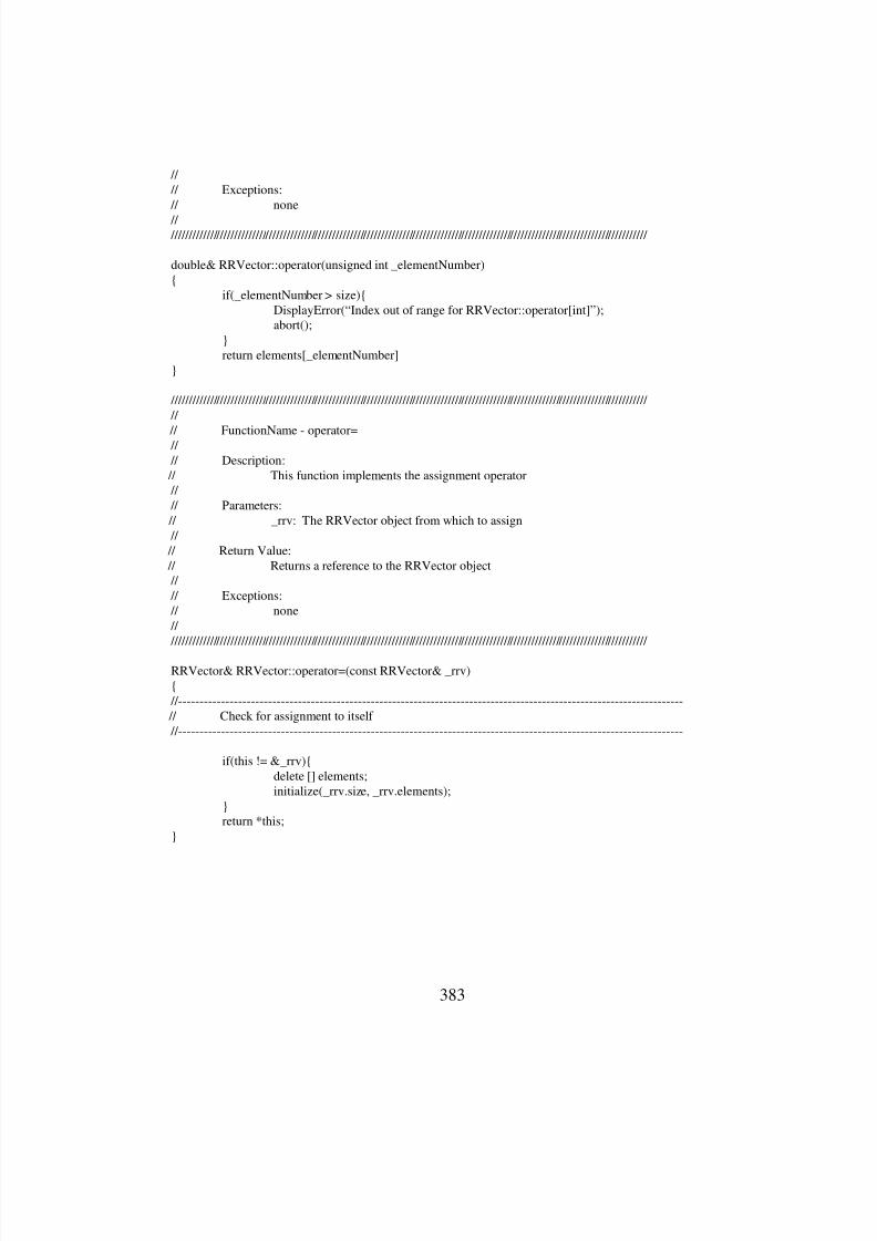
8/3/2019 Chetan Kapoor Dissertation
http://slidepdf.com/reader/full/chetan-kapoor-dissertation 404/612
383
// // Exceptions: // none
// ////////////////////////////////////////////////////////////////////////////////////////////////////////////////////////////////////////
double& RRVector::operator(unsigned int _elementNumber){
if(_elementNumber > size){DisplayError(“Index out of range for RRVector::operator[int]”);abort();
}return elements[_elementNumber]
}
//////////////////////////////////////////////////////////////////////////////////////////////////////////////////////////////////////// //
// FunctionName - operator= // // Description: // This function implements the assignment operator // // Parameters: // _rrv: The RRVector object from which to assign // // Return Value: // Returns a reference to the RRVector object // // Exceptions: // none // ////////////////////////////////////////////////////////////////////////////////////////////////////////////////////////////////////////
RRVector& RRVector::operator=(const RRVector& _rrv){
//---------------------------------------------------------------------------------------------------------------------- // Check for assignment to itself //----------------------------------------------------------------------------------------------------------------------
if(this != &_rrv){delete [] elements;initialize(_rrv.size, _rrv.elements);
}return *this;
}
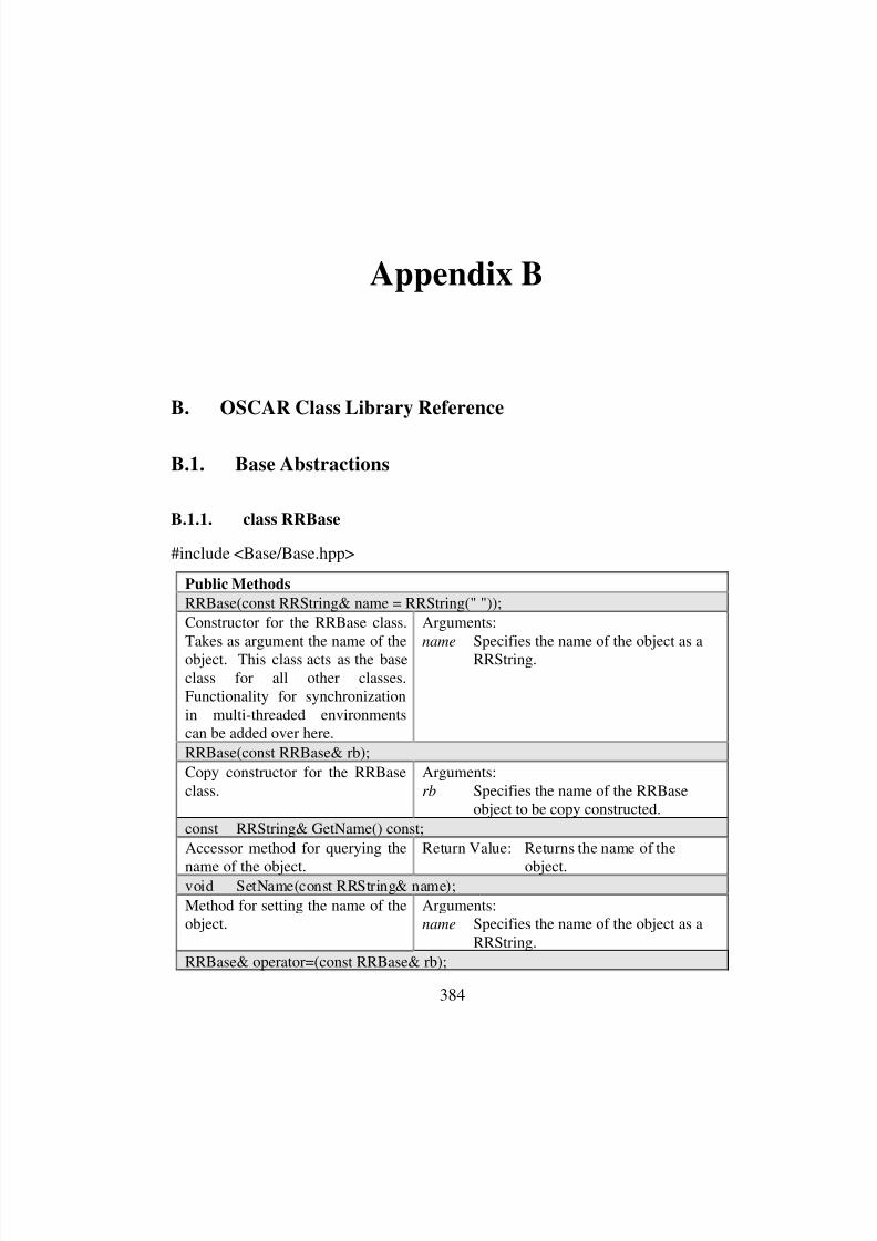
8/3/2019 Chetan Kapoor Dissertation
http://slidepdf.com/reader/full/chetan-kapoor-dissertation 405/612
384
Appendix B
B. OSCAR Class Library Reference
B.1. Base Abstractions
B.1.1. class RRBase
#include <Base/Base.hpp>
Public Methods
RRBase(const RRString& name = RRString(" "));
Constructor for the RRBase class.Takes as argument the name of theobject. This class acts as the baseclass for all other classes.Functionality for synchronizationin multi-threaded environmentscan be added over here.
Arguments:
name Specifies the name of the object as aRRString.
RRBase(const RRBase& rb);
Copy constructor for the RRBaseclass.
Arguments:
rb Specifies the name of the RRBaseobject to be copy constructed.
const RRString& GetName() const;
Accessor method for querying the
name of the object.
Return Value: Returns the name of the
object.void SetName(const RRString& name);
Method for setting the name of theobject.
Arguments:name Specifies the name of the object as a
RRString.
RRBase& operator=(const RRBase& rb);

8/3/2019 Chetan Kapoor Dissertation
http://slidepdf.com/reader/full/chetan-kapoor-dissertation 406/612
385
Operator overload for copying anRRBase object.
Arguments:rb Specifies the object to be copied.
Return Value: Returns a reference to itself.
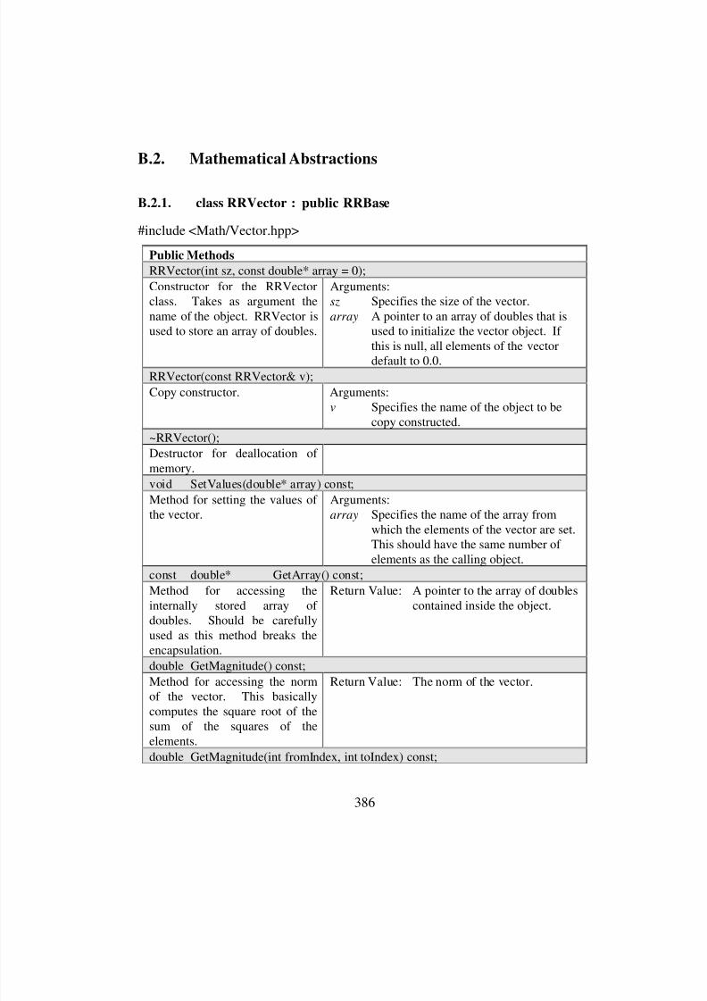
8/3/2019 Chetan Kapoor Dissertation
http://slidepdf.com/reader/full/chetan-kapoor-dissertation 407/612
386
B.2. Mathematical Abstractions
B.2.1. class RRVector : public RRBase
#include <Math/Vector.hpp>
Public Methods
RRVector(int sz, const double* array = 0);
Constructor for the RRVectorclass. Takes as argument thename of the object. RRVector isused to store an array of doubles.
Arguments:sz Specifies the size of the vector.
array A pointer to an array of doubles that isused to initialize the vector object. If
this is null, all elements of the vectordefault to 0.0.
RRVector(const RRVector& v);
Copy constructor. Arguments:v Specifies the name of the object to be
copy constructed.
~RRVector();
Destructor for deallocation of memory.
void SetValues(double* array) const;
Method for setting the values of the vector.
Arguments:array Specifies the name of the array from
which the elements of the vector are set.This should have the same number of elements as the calling object.
const double* GetArray() const;
Method for accessing theinternally stored array of doubles. Should be carefullyused as this method breaks theencapsulation.
Return Value: A pointer to the array of doublescontained inside the object.
double GetMagnitude() const;
Method for accessing the norm
of the vector. This basicallycomputes the square root of thesum of the squares of theelements.
Return Value: The norm of the vector.
double GetMagnitude(int fromIndex, int toIndex) const;
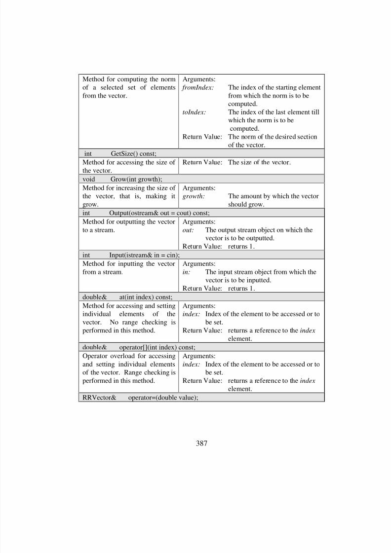
8/3/2019 Chetan Kapoor Dissertation
http://slidepdf.com/reader/full/chetan-kapoor-dissertation 408/612
387
Method for computing the normof a selected set of elements
from the vector.
Arguments: fromIndex: The index of the starting element
from which the norm is to becomputed.
toIndex: The index of the last element tillwhich the norm is to becomputed.
Return Value: The norm of the desired sectionof the vector.
int GetSize() const;
Method for accessing the size of the vector.
Return Value: The size of the vector.
void Grow(int growth);
Method for increasing the size of
the vector, that is, making itgrow.
Arguments:
growth: The amount by which the vectorshould grow.
int Output(ostream& out = cout) const;
Method for outputting the vectorto a stream.
Arguments:
out: The output stream object on which thevector is to be outputted.
Return Value: returns 1.
int Input(istream& in = cin);
Method for inputting the vectorfrom a stream.
Arguments:
in: The input stream object from which thevector is to be inputted.
Return Value: returns 1.double& at(int index) const;
Method for accessing and settingindividual elements of thevector. No range checking isperformed in this method.
Arguments:index: Index of the element to be accessed or to
be set.Return Value: returns a reference to the index
element.
double& operator[](int index) const;
Operator overload for accessingand setting individual elementsof the vector. Range checking isperformed in this method.
Arguments:
index: Index of the element to be accessed or tobe set.
Return Value: returns a reference to the index
element.RRVector& operator=(double value);

8/3/2019 Chetan Kapoor Dissertation
http://slidepdf.com/reader/full/chetan-kapoor-dissertation 409/612
388
Operator overload for ‘=’ forsetting all the elements of a
vector to a particular number.
Arguments:value: Number to which all the elements of the
vector should be set.Return Value: returns a reference to the vector
being set.
int operator==(const RRVector& v) const;
Comparison method. Arguments:
v: RRVector with which the comparison isto be made.
Return Value: Returns 1 if equal and 0 if not.
RRVector operator*(double number);
Method to multiply an RRVectorwith a double.
Arguments:number: The number with which all the
elements of the RRVector are to
be multiplied.Return Value: The resulting RRVector.
RRVector& operator*=(double number);
Method to multiply all itselements with a double.
Arguments:
number: The number with which all theelements of the RRVector are tobe multiplied.
Return Value: Returns a reference to self.
RRVector& operator+=(double number);
Method to add a double to all itselements.
Arguments:number: The number which has to be
added to all the elements.Return Value: Returns a reference to self.
RRVector& operator/=(double number);
Method to divide all its elementswith a double.
Arguments:
number: The number with which all theelements of the RRVector are tobe divided.
Return Value: Returns a reference to self.
RRVector& operator-=(double number);
Method to subtract a doublefrom all its elements.
Arguments:number: The number which has to be
subtracted from all the elements.
Return Value: Returns a reference to self.RRVector& operator+=(const RRVector& v);
Method to add anotherRRVector to self.
Arguments:v: The RRVector that has to be added.Return Value: Returns a reference to self.
RRVector& operator-=(const RRVector& v);
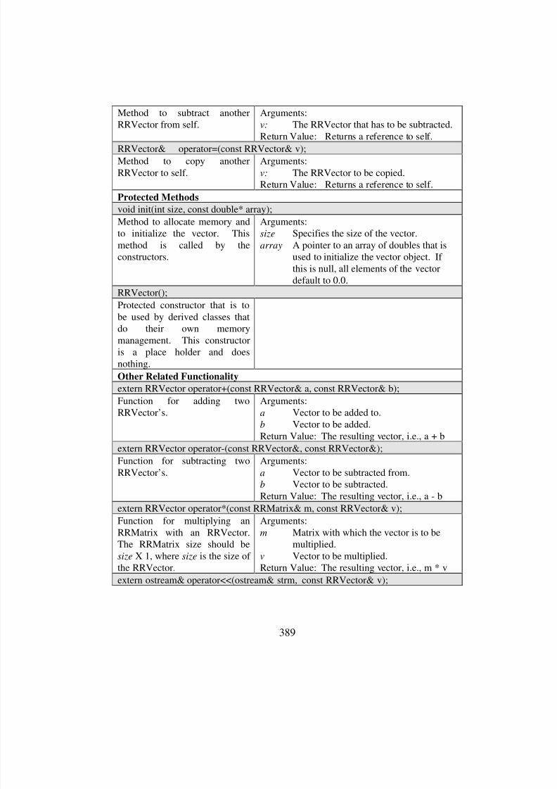
8/3/2019 Chetan Kapoor Dissertation
http://slidepdf.com/reader/full/chetan-kapoor-dissertation 410/612
389
Method to subtract anotherRRVector from self.
Arguments:v: The RRVector that has to be subtracted.
Return Value: Returns a reference to self.RRVector& operator=(const RRVector& v);
Method to copy anotherRRVector to self.
Arguments:
v: The RRVector to be copied.Return Value: Returns a reference to self.
Protected Methods
void init(int size, const double* array);
Method to allocate memory andto initialize the vector. Thismethod is called by theconstructors.
Arguments:size Specifies the size of the vector.
array A pointer to an array of doubles that isused to initialize the vector object. If this is null, all elements of the vector
default to 0.0.
RRVector();
Protected constructor that is tobe used by derived classes thatdo their own memorymanagement. This constructoris a place holder and doesnothing.
Other Related Functionality
extern RRVector operator+(const RRVector& a, const RRVector& b);
Function for adding two
RRVector’s.
Arguments:
a Vector to be added to.b Vector to be added.Return Value: The resulting vector, i.e., a + b
extern RRVector operator-(const RRVector&, const RRVector&);
Function for subtracting twoRRVector’s.
Arguments:
a Vector to be subtracted from.b Vector to be subtracted.Return Value: The resulting vector, i.e., a - b
extern RRVector operator*(const RRMatrix& m, const RRVector& v);
Function for multiplying anRRMatrix with an RRVector.The RRMatrix size should be
size X 1, where size is the size of the RRVector.
Arguments:
m Matrix with which the vector is to bemultiplied.
v Vector to be multiplied.Return Value: The resulting vector, i.e., m * v
extern ostream& operator<<(ostream& strm, const RRVector& v);
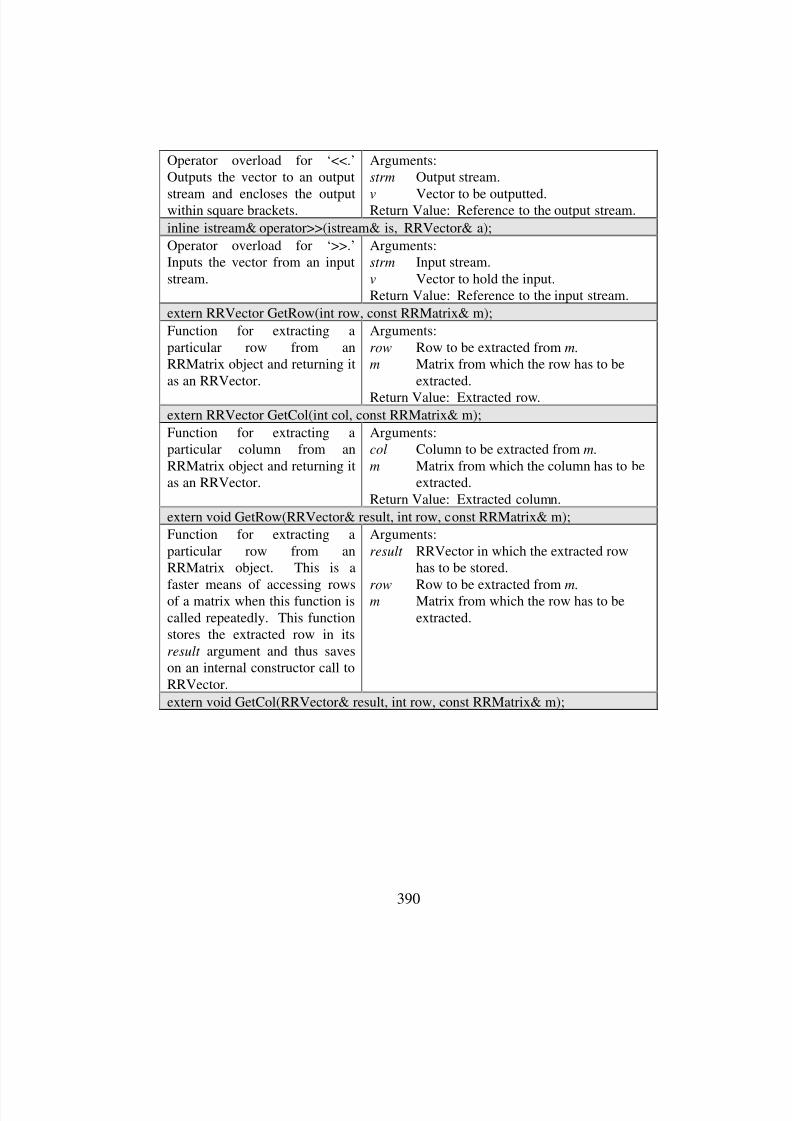
8/3/2019 Chetan Kapoor Dissertation
http://slidepdf.com/reader/full/chetan-kapoor-dissertation 411/612
390
Operator overload for ‘<<.’Outputs the vector to an output
stream and encloses the outputwithin square brackets.
Arguments:strm Output stream.
v Vector to be outputted.Return Value: Reference to the output stream.
inline istream& operator>>(istream& is, RRVector& a);
Operator overload for ‘>>.’Inputs the vector from an inputstream.
Arguments:strm Input stream.
v Vector to hold the input.Return Value: Reference to the input stream.
extern RRVector GetRow(int row, const RRMatrix& m);
Function for extracting aparticular row from anRRMatrix object and returning itas an RRVector.
Arguments:
row Row to be extracted from m.
m Matrix from which the row has to beextracted.
Return Value: Extracted row.extern RRVector GetCol(int col, const RRMatrix& m);
Function for extracting aparticular column from anRRMatrix object and returning itas an RRVector.
Arguments:col Column to be extracted from m.
m Matrix from which the column has to beextracted.
Return Value: Extracted column.
extern void GetRow(RRVector& result, int row, const RRMatrix& m);
Function for extracting aparticular row from anRRMatrix object. This is a
faster means of accessing rowsof a matrix when this function iscalled repeatedly. This functionstores the extracted row in its
result argument and thus saveson an internal constructor call toRRVector.
Arguments:
result RRVector in which the extracted rowhas to be stored.
row Row to be extracted from m.m Matrix from which the row has to be
extracted.
extern void GetCol(RRVector& result, int row, const RRMatrix& m);
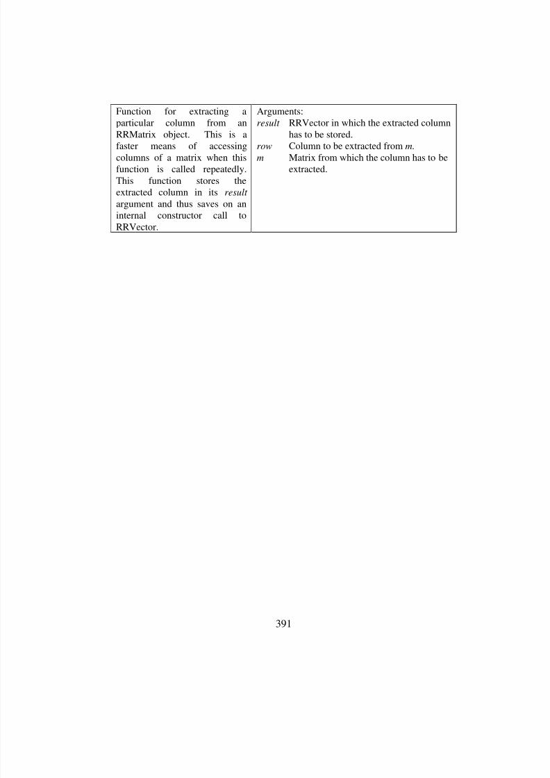
8/3/2019 Chetan Kapoor Dissertation
http://slidepdf.com/reader/full/chetan-kapoor-dissertation 412/612
391
Function for extracting aparticular column from an
RRMatrix object. This is afaster means of accessingcolumns of a matrix when thisfunction is called repeatedly.This function stores theextracted column in its result
argument and thus saves on aninternal constructor call toRRVector.
Arguments:result RRVector in which the extracted column
has to be stored.row Column to be extracted from m.
m Matrix from which the column has to beextracted.
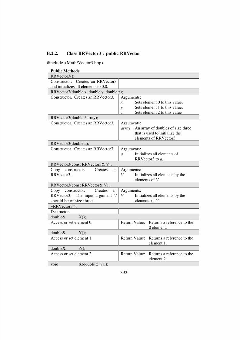
8/3/2019 Chetan Kapoor Dissertation
http://slidepdf.com/reader/full/chetan-kapoor-dissertation 413/612
392
B.2.2. Class RRVector3 : public RRVector
#include <Math/Vector3.hpp>
Public Methods
RRVector3();
Constructor. Creates an RRVector3and initializes all elements to 0.0.
RRVector3(double x, double y, double z);
Constructor. Creates an RRVector3. Arguments: x Sets element 0 to this value.
y Sets element 1 to this value. z Sets element 2 to this value
RRVector3(double *array);Constructor. Creates an RRVector3. Arguments:
array An array of doubles of size threethat is used to initialize theelements of RRVector3.
RRVector3(double a);
Constructor. Creates an RRVector3. Arguments:
a Initializes all elements of RRVector3 to a.
RRVector3(const RRVector3& V);
Copy constructor. Creates anRRVector3.
Arguments:V Initializes all elements by the
elements of V.RRVector3(const RRVector& V);
Copy constructor. Creates anRRVector3. The input argument V
should be of size three.
Arguments:
V Initializes all elements by theelements of V.
~RRVector3();
Destructor.
double& X();
Access or set element 0. Return Value: Returns a reference to the0 element.
double& Y();
Access or set element 1. Return Value: Returns a reference to theelement 1.
double& Z();
Access or set element 2. Return Value: Returns a reference to theelement 2.
void X(double x_val);
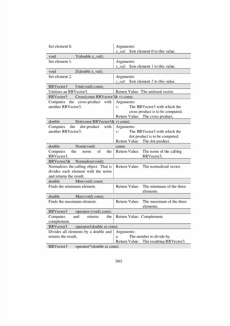
8/3/2019 Chetan Kapoor Dissertation
http://slidepdf.com/reader/full/chetan-kapoor-dissertation 414/612
393
Set element 0. Arguments:
x_val: Sets element 0 to this value.
void Y(double y_val);Set element 1. Arguments:
y_val: Sets element 1 to this value.
void Z(double z_val);
Set element 2. Arguments: z_val: Sets element 2 to this value.
RRVector3 Unit(void) const;
Unitizes an RRVector3. Return Value: The unitized vector.
RRVector3 Cross(const RRVector3& v) const;
Computes the cross-product withanother RRVector3.
Arguments:
v: The RRVector3 with which thecross product is to be computed.
Return Value: The cross product.
double Dot(const RRVector3& v) const;
Computes the dot-product withanother RRVector3.
Arguments:v: The RRVector3 with which the
dot product is to be computed.Return Value: The dot product.
double Norm(void) const;
Computes the norm of theRRVector3.
Return Value: The norm of the callingRRVector3.
RRVector3& Normalize(void);
Normalizes the calling object. That is
divides each element with the normand returns the result.
Return Value: The normalized vector.
double Min(void) const;
Finds the minimum element. Return Value: The minimum of the threeelements.
double Max(void) const;
Finds the maximum element. Return Value: The maximum of the threeelements.
RRVector3 operator-(void) const;
Computes and returns thecomplement.
Return Value: Complement.
RRVector3 operator/(double a) const;Divides all elements by a double andreturns the result.
Arguments:a The number to divide by.Return Value: The resulting RRVector3.
RRVector3 operator*(double a) const;
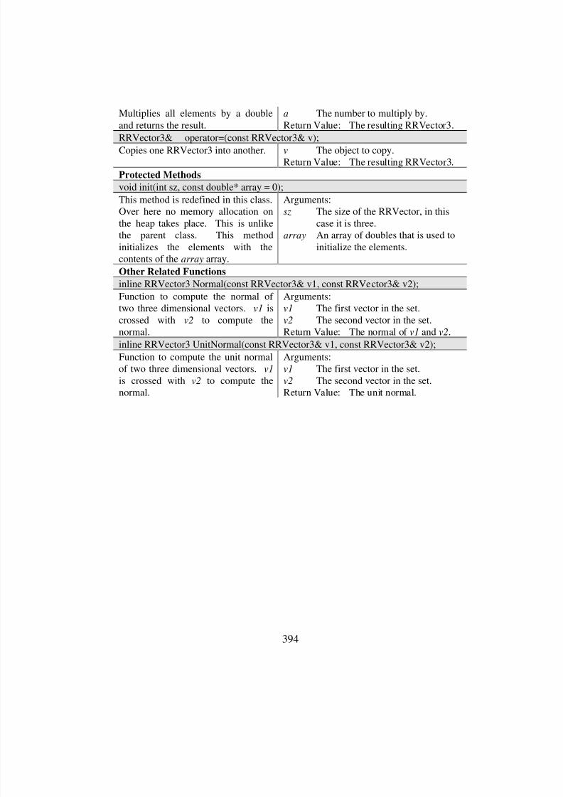
8/3/2019 Chetan Kapoor Dissertation
http://slidepdf.com/reader/full/chetan-kapoor-dissertation 415/612
394
Multiplies all elements by a doubleand returns the result.
a The number to multiply by.Return Value: The resulting RRVector3.
RRVector3& operator=(const RRVector3& v);Copies one RRVector3 into another. v The object to copy.
Return Value: The resulting RRVector3.
Protected Methods
void init(int sz, const double* array = 0);
This method is redefined in this class.Over here no memory allocation onthe heap takes place. This is unlikethe parent class. This methodinitializes the elements with thecontents of the array array.
Arguments:sz The size of the RRVector, in this
case it is three.array An array of doubles that is used to
initialize the elements.
Other Related Functions
inline RRVector3 Normal(const RRVector3& v1, const RRVector3& v2);
Function to compute the normal of two three dimensional vectors. v1 iscrossed with v2 to compute thenormal.
Arguments:v1 The first vector in the set.
v2 The second vector in the set.Return Value: The normal of v1 and v2.
inline RRVector3 UnitNormal(const RRVector3& v1, const RRVector3& v2);
Function to compute the unit normalof two three dimensional vectors. v1
is crossed with v2 to compute thenormal.
Arguments:v1 The first vector in the set.
v2 The second vector in the set.Return Value: The unit normal.
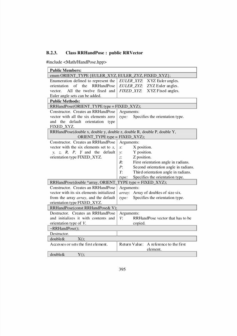
8/3/2019 Chetan Kapoor Dissertation
http://slidepdf.com/reader/full/chetan-kapoor-dissertation 416/612
395
B.2.3. Class RRHandPose : public RRVector
#include <Math/HandPose.hpp>
Public Members:
enum ORIENT_TYPE {EULER_XYZ, EULER_ZYZ, FIXED_XYZ};
Enumeration defined to represent theorientation of the RRHandPosevector. All the twelve fixed andEuler angle sets can be added.
EULER_XYZ : XYZ Euler angles.
EULER_ZYZ : ZYZ Euler angles.FIXED_XYZ : XYZ Fixed angles.
Public Methods:
RRHandPose(ORIENT_TYPE type = FIXED_XYZ);
Constructor. Creates an RRHandPose
vector with all the six elements zeroand the default orientation typeFIXED_XYZ.
Arguments:
type: Specifies the orientation type.
RRHandPose(double x, double y, double z, double R, double P, double Y,ORIENT_TYPE type = FIXED_XYZ);
Constructor. Creates an RRHandPosevector with the six elements set to x,
y, z, R, P, Y , and the defaultorientation type FIXED_XYZ.
Arguments: x: X position.
y: Y position. z: Z position.
R: First orientation angle in radians.P: Second orientation angle in radians.
Y : Third orientation angle in radians.
type: Specifies the orientation type.RRHandPose(double *array, ORIENT_TYPE type = FIXED_XYZ);
Constructor. Creates an RRHandPosevector with its six elements initializedfrom the array array, and the defaultorientation type FIXED_XYZ.
Arguments:array: Array of doubles of size six.
type: Specifies the orientation type.
RRHandPose(const RRHandPose& V);
Destructor. Creates an RRHandPoseand initializes it with contents andorientation type of V .
Arguments:V : RRHandPose vector that has to be
copied.
~RRHandPose();
Destructor.double& X();
Accesses or sets the first element. Return Value: A reference to the firstelement.
double& Y();
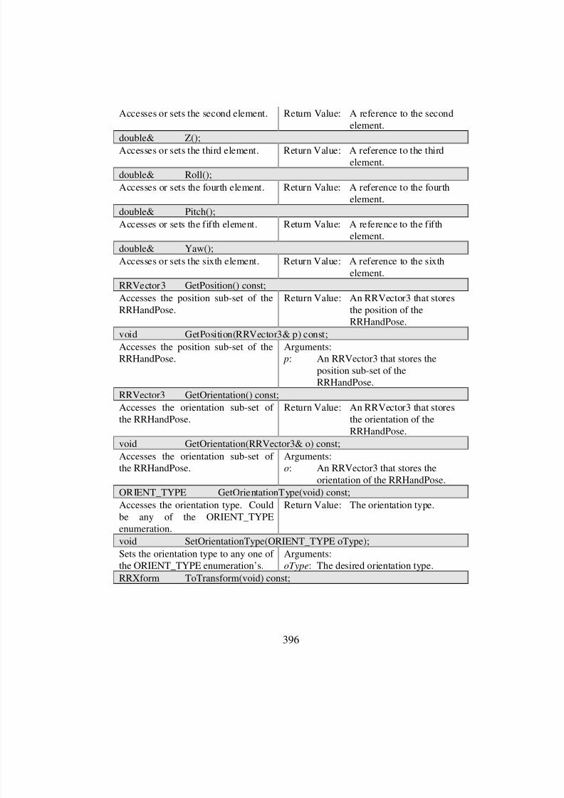
8/3/2019 Chetan Kapoor Dissertation
http://slidepdf.com/reader/full/chetan-kapoor-dissertation 417/612
396
Accesses or sets the second element. Return Value: A reference to the secondelement.
double& Z();Accesses or sets the third element. Return Value: A reference to the third
element.
double& Roll();
Accesses or sets the fourth element. Return Value: A reference to the fourthelement.
double& Pitch();
Accesses or sets the fifth element. Return Value: A reference to the fifthelement.
double& Yaw();
Accesses or sets the sixth element. Return Value: A reference to the sixthelement.
RRVector3 GetPosition() const;
Accesses the position sub-set of theRRHandPose.
Return Value: An RRVector3 that storesthe position of theRRHandPose.
void GetPosition(RRVector3& p) const;
Accesses the position sub-set of theRRHandPose.
Arguments: p: An RRVector3 that stores the
position sub-set of theRRHandPose.
RRVector3 GetOrientation() const;
Accesses the orientation sub-set of
the RRHandPose.
Return Value: An RRVector3 that stores
the orientation of theRRHandPose.
void GetOrientation(RRVector3& o) const;
Accesses the orientation sub-set of the RRHandPose.
Arguments:o: An RRVector3 that stores the
orientation of the RRHandPose.
ORIENT_TYPE GetOrientationType(void) const;
Accesses the orientation type. Couldbe any of the ORIENT_TYPEenumeration.
Return Value: The orientation type.
void SetOrientationType(ORIENT_TYPE oType);
Sets the orientation type to any one of the ORIENT_TYPE enumeration’s.
Arguments:oType: The desired orientation type.
RRXform ToTransform(void) const;
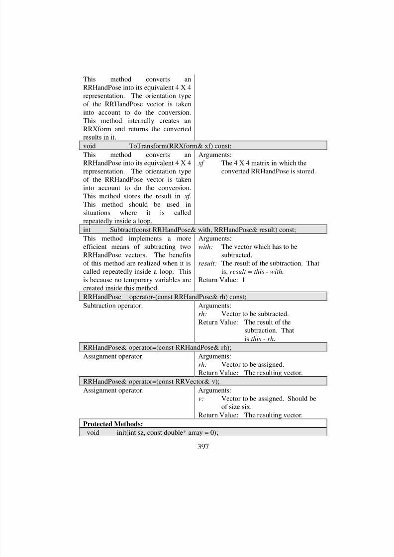
8/3/2019 Chetan Kapoor Dissertation
http://slidepdf.com/reader/full/chetan-kapoor-dissertation 418/612
397
This method converts anRRHandPose into its equivalent 4 X 4
representation. The orientation typeof the RRHandPose vector is takeninto account to do the conversion.This method internally creates anRRXform and returns the convertedresults in it.
void ToTransform(RRXform& xf) const;
This method converts anRRHandPose into its equivalent 4 X 4representation. The orientation typeof the RRHandPose vector is takeninto account to do the conversion.
This method stores the result in xf .This method should be used insituations where it is calledrepeatedly inside a loop.
Arguments: xf The 4 X 4 matrix in which the
converted RRHandPose is stored.
int Subtract(const RRHandPose& with, RRHandPose& result) const;
This method implements a moreefficient means of subtracting twoRRHandPose vectors. The benefitsof this method are realized when it iscalled repeatedly inside a loop. Thisis because no temporary variables arecreated inside this method.
Arguments:
with: The vector which has to besubtracted.
result: The result of the subtraction. Thatis, result = this - with.
Return Value: 1
RRHandPose operator-(const RRHandPose& rh) const;
Subtraction operator. Arguments:rh: Vector to be subtracted.Return Value: The result of the
subtraction. Thatis this - rh.
RRHandPose& operator=(const RRHandPose& rh);
Assignment operator. Arguments:rh: Vector to be assigned.Return Value: The resulting vector.
RRHandPose& operator=(const RRVector& v);
Assignment operator. Arguments:v: Vector to be assigned. Should be
of size six.Return Value: The resulting vector.
Protected Methods:
void init(int sz, const double* array = 0);
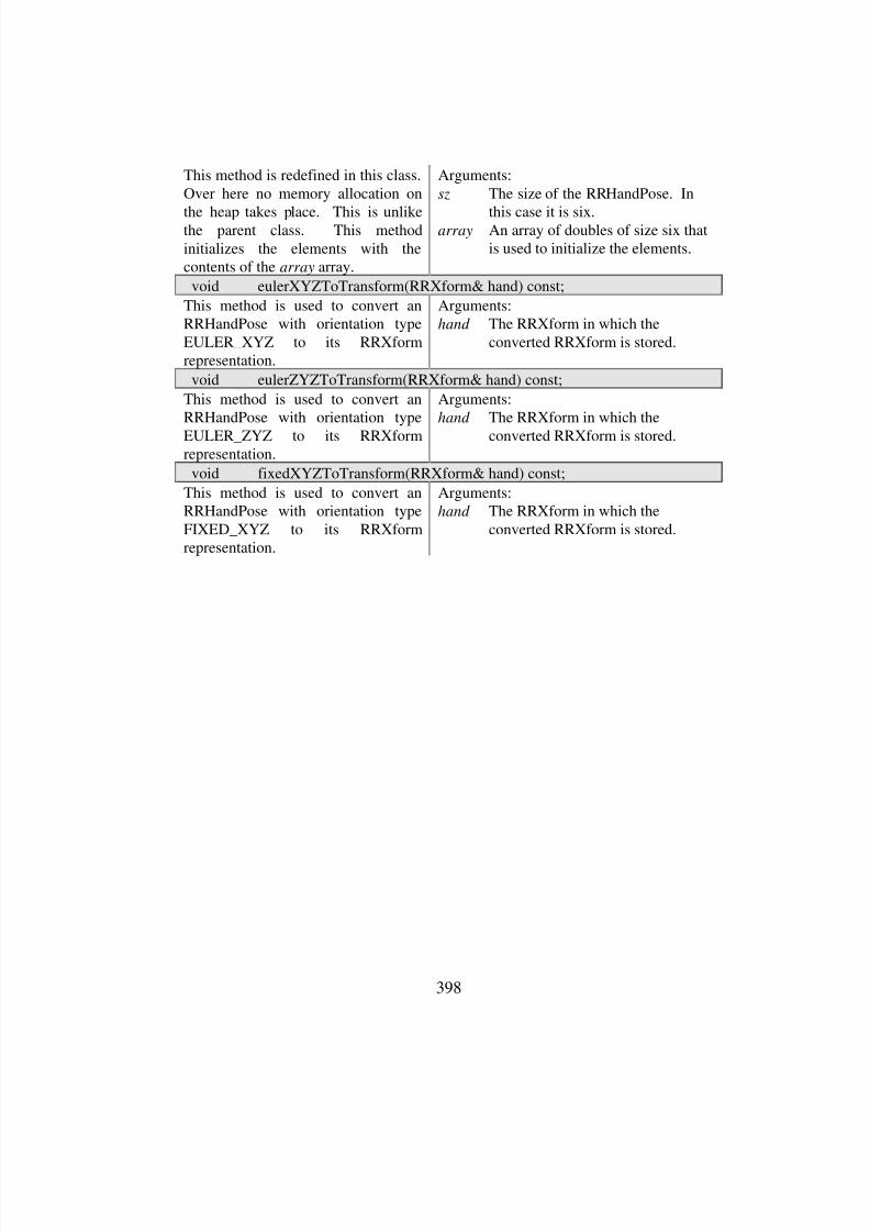
8/3/2019 Chetan Kapoor Dissertation
http://slidepdf.com/reader/full/chetan-kapoor-dissertation 419/612
398
This method is redefined in this class.Over here no memory allocation on
the heap takes place. This is unlikethe parent class. This methodinitializes the elements with thecontents of the array array.
Arguments:
sz The size of the RRHandPose. In
this case it is six.array An array of doubles of size six that
is used to initialize the elements.
void eulerXYZToTransform(RRXform& hand) const;
This method is used to convert anRRHandPose with orientation typeEULER_XYZ to its RRXformrepresentation.
Arguments:hand The RRXform in which the
converted RRXform is stored.
void eulerZYZToTransform(RRXform& hand) const;
This method is used to convert anRRHandPose with orientation type
EULER_ZYZ to its RRXformrepresentation.
Arguments:hand The RRXform in which the
converted RRXform is stored.
void fixedXYZToTransform(RRXform& hand) const;
This method is used to convert anRRHandPose with orientation typeFIXED_XYZ to its RRXformrepresentation.
Arguments:hand The RRXform in which the
converted RRXform is stored.
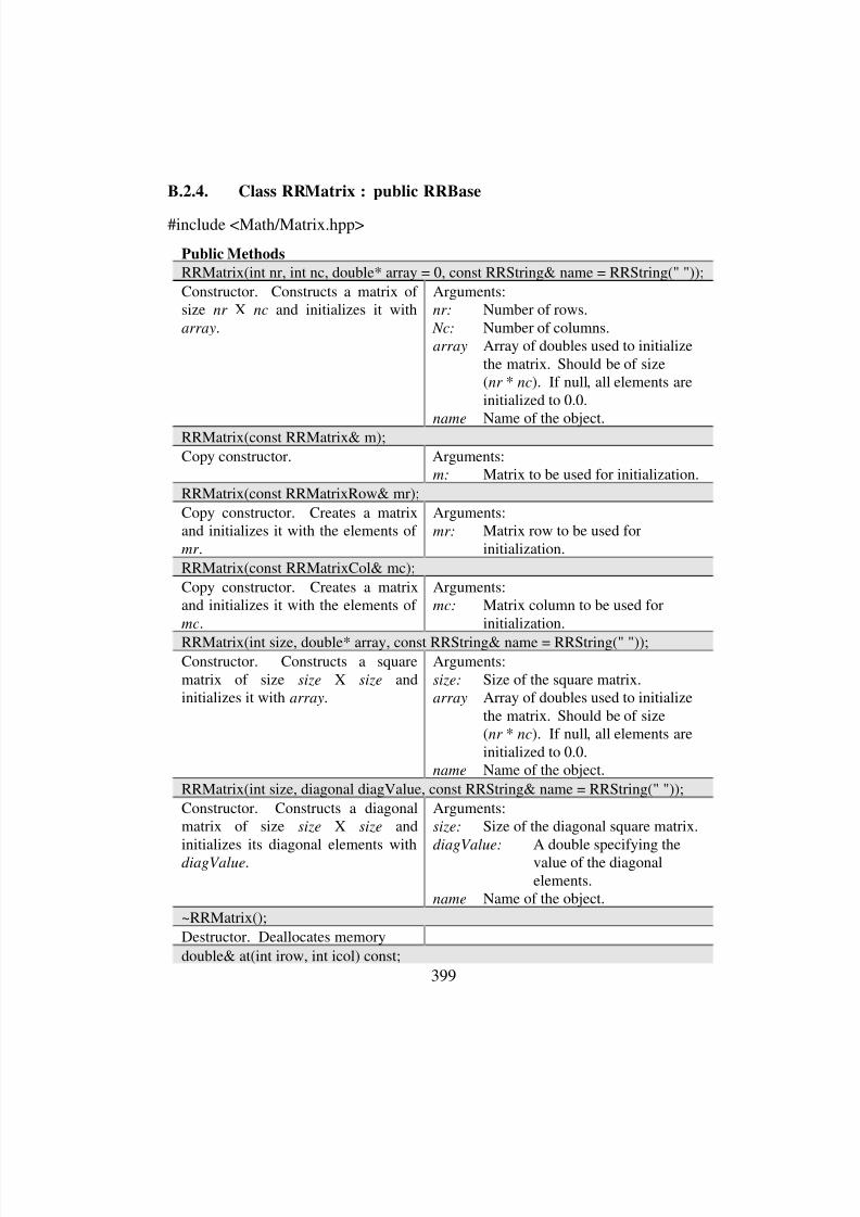
8/3/2019 Chetan Kapoor Dissertation
http://slidepdf.com/reader/full/chetan-kapoor-dissertation 420/612
399
B.2.4. Class RRMatrix : public RRBase
#include <Math/Matrix.hpp>
Public Methods
RRMatrix(int nr, int nc, double* array = 0, const RRString& name = RRString(" "));
Constructor. Constructs a matrix of size nr X nc and initializes it with
array.
Arguments:nr: Number of rows.
Nc: Number of columns.array Array of doubles used to initialize
the matrix. Should be of size(nr * nc). If null, all elements areinitialized to 0.0.
name Name of the object.
RRMatrix(const RRMatrix& m);
Copy constructor. Arguments:m: Matrix to be used for initialization.
RRMatrix(const RRMatrixRow& mr);
Copy constructor. Creates a matrixand initializes it with the elements of
mr .
Arguments:
mr: Matrix row to be used forinitialization.
RRMatrix(const RRMatrixCol& mc);
Copy constructor. Creates a matrixand initializes it with the elements of
mc.
Arguments:mc: Matrix column to be used for
initialization.
RRMatrix(int size, double* array, const RRString& name = RRString(" "));Constructor. Constructs a squarematrix of size size X size andinitializes it with array.
Arguments:
size: Size of the square matrix.array Array of doubles used to initialize
the matrix. Should be of size(nr * nc). If null, all elements areinitialized to 0.0.
name Name of the object.
RRMatrix(int size, diagonal diagValue, const RRString& name = RRString(" "));
Constructor. Constructs a diagonalmatrix of size size X size andinitializes its diagonal elements withdiagValue.
Arguments:size: Size of the diagonal square matrix.
diagValue: A double specifying thevalue of the diagonalelements.
name Name of the object.
~RRMatrix();
Destructor. Deallocates memory
double& at(int irow, int icol) const;
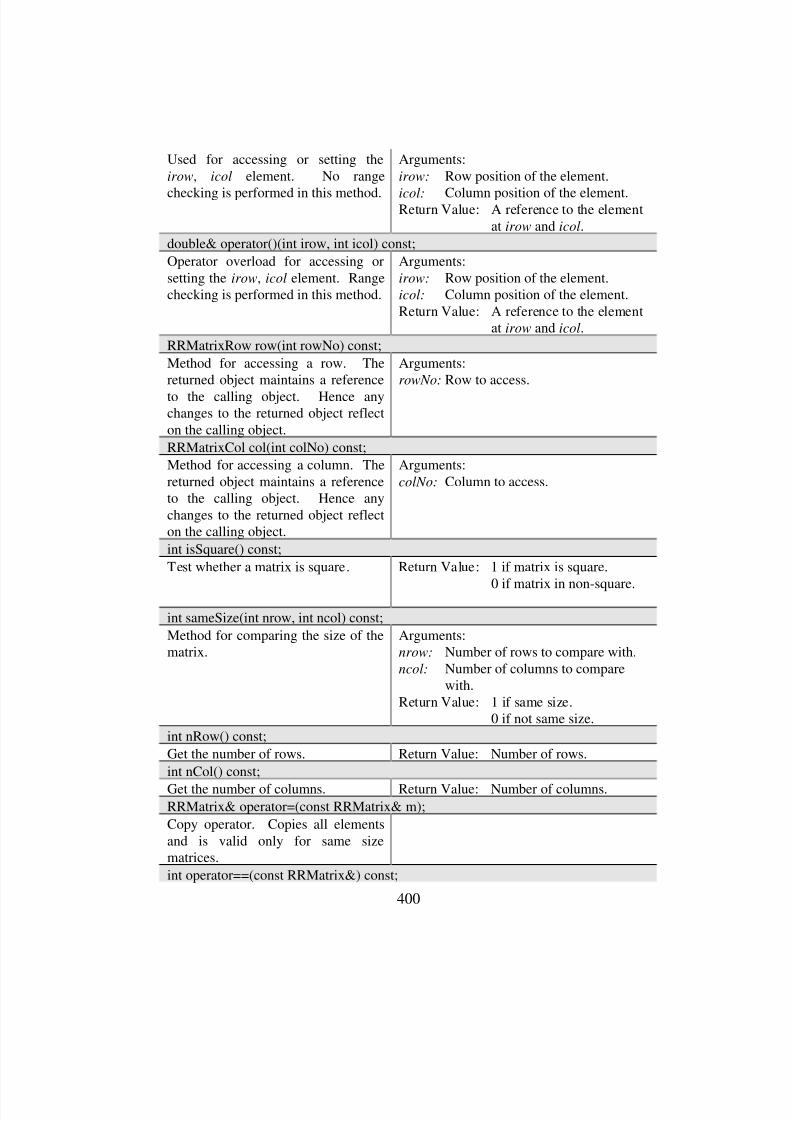
8/3/2019 Chetan Kapoor Dissertation
http://slidepdf.com/reader/full/chetan-kapoor-dissertation 421/612
400
Used for accessing or setting the
irow, icol element. No range
checking is performed in this method.
Arguments:
irow: Row position of the element.
icol: Column position of the element.Return Value: A reference to the element
at irow and icol.
double& operator()(int irow, int icol) const;
Operator overload for accessing orsetting the irow, icol element. Rangechecking is performed in this method.
Arguments:
irow: Row position of the element.icol: Column position of the element.Return Value: A reference to the element
at irow and icol.
RRMatrixRow row(int rowNo) const;
Method for accessing a row. Thereturned object maintains a reference
to the calling object. Hence anychanges to the returned object reflecton the calling object.
Arguments:rowNo: Row to access.
RRMatrixCol col(int colNo) const;
Method for accessing a column. Thereturned object maintains a referenceto the calling object. Hence anychanges to the returned object reflecton the calling object.
Arguments:
colNo: Column to access.
int isSquare() const;
Test whether a matrix is square. Return Value: 1 if matrix is square.
0 if matrix in non-square.
int sameSize(int nrow, int ncol) const;
Method for comparing the size of thematrix.
Arguments:nrow: Number of rows to compare with.
ncol: Number of columns to comparewith.
Return Value: 1 if same size.0 if not same size.
int nRow() const;
Get the number of rows. Return Value: Number of rows.
int nCol() const;
Get the number of columns. Return Value: Number of columns.RRMatrix& operator=(const RRMatrix& m);
Copy operator. Copies all elementsand is valid only for same sizematrices.
int operator==(const RRMatrix&) const;
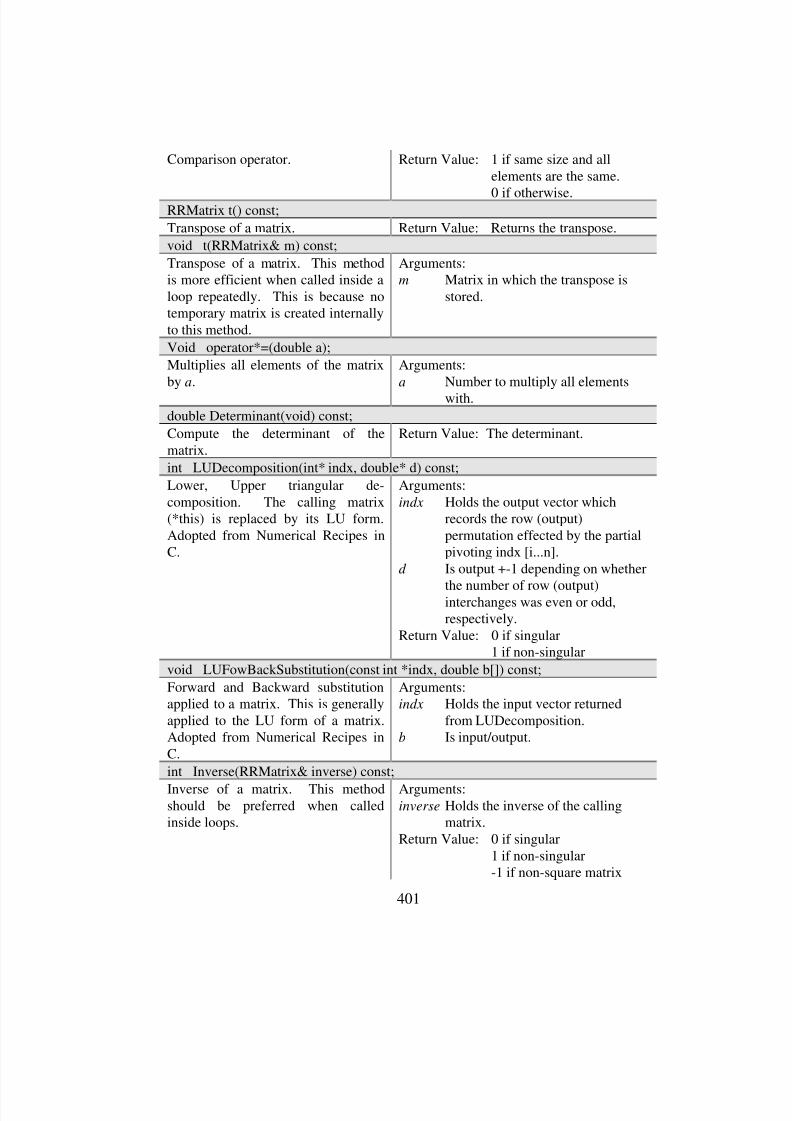
8/3/2019 Chetan Kapoor Dissertation
http://slidepdf.com/reader/full/chetan-kapoor-dissertation 422/612
401
Comparison operator. Return Value: 1 if same size and allelements are the same.
0 if otherwise.RRMatrix t() const;
Transpose of a matrix. Return Value: Returns the transpose.
void t(RRMatrix& m) const;
Transpose of a matrix. This methodis more efficient when called inside aloop repeatedly. This is because notemporary matrix is created internallyto this method.
Arguments:m Matrix in which the transpose is
stored.
Void operator*=(double a);
Multiplies all elements of the matrixby a.
Arguments:
a Number to multiply all elements
with.
double Determinant(void) const;
Compute the determinant of thematrix.
Return Value: The determinant.
int LUDecomposition(int* indx, double* d) const;
Lower, Upper triangular de-composition. The calling matrix(*this) is replaced by its LU form.Adopted from Numerical Recipes inC.
Arguments:
indx Holds the output vector whichrecords the row (output)permutation effected by the partialpivoting indx [i...n].
d Is output +-1 depending on whether
the number of row (output)interchanges was even or odd,respectively.
Return Value: 0 if singular1 if non-singular
void LUFowBackSubstitution(const int *indx, double b[]) const;
Forward and Backward substitutionapplied to a matrix. This is generallyapplied to the LU form of a matrix.Adopted from Numerical Recipes inC.
Arguments:indx Holds the input vector returned
from LUDecomposition.b Is input/output.
int Inverse(RRMatrix& inverse) const;
Inverse of a matrix. This methodshould be preferred when calledinside loops.
Arguments:inverse Holds the inverse of the calling
matrix.Return Value: 0 if singular
1 if non-singular-1 if non-square matrix

8/3/2019 Chetan Kapoor Dissertation
http://slidepdf.com/reader/full/chetan-kapoor-dissertation 423/612
402
int Inverse(RRMatrix& inverse, double& determinant) const;
Inverse and determinant of a matrix.
This method should be preferredwhen called inside loops.
Arguments:
inverse Holds the inverse of the callingmatrix.
determinant The determinant of thecalling matrix.
Return Value: 0 if singular1 if non-singular-1 if non-square matrix
int SpeedInverse(RRMatrix& inverse, double& determinant) const;
Inverse and determinant of a matrix.This method should be preferredwhen called inside loops and is fasterthan the previous method. However,
this method destroys the callingmatrix.
Arguments:
inverse Holds the inverse of the callingmatrix.
determinant The determinant of the
calling matrix.Return Value: 0 if singular
1 if non-singular-1 if non-square matrix
int SVD(RRMatrix& U, RRVector& V, RRMatrix W) const;
Computes the singular valuedecomposition of the calling matrixwhose size is m X n. Adopted fromNumerical Recipes in C.
Arguments:U matrix of size m X n if m >= n or
matrix of size n X n if m < nV Vector of size n that holds
the Eigen ValuesW matrix of size n X nReturn Value: 0 if no convergence
1 if successful
RRMatrix Inverse() const;
Inverse of a matrix. Return Value: The inverse.
void MultiplyWithTranspose(RRMatrix& result) const;
Multiplies the calling matrix with itstranspose.
Arguments:
result The result of multiplying the callingmatrix with its transpose.
void switchRows(int a, int b);
Switch two rows of a matrix Arguments:
a, b Numbers of the rows to beswitched.
void switchCols(int a, int b);Switch two columns of a matrix Arguments:
a, b Numbers of the columns to beswitched.
void combineRows(int i, double b, int j);
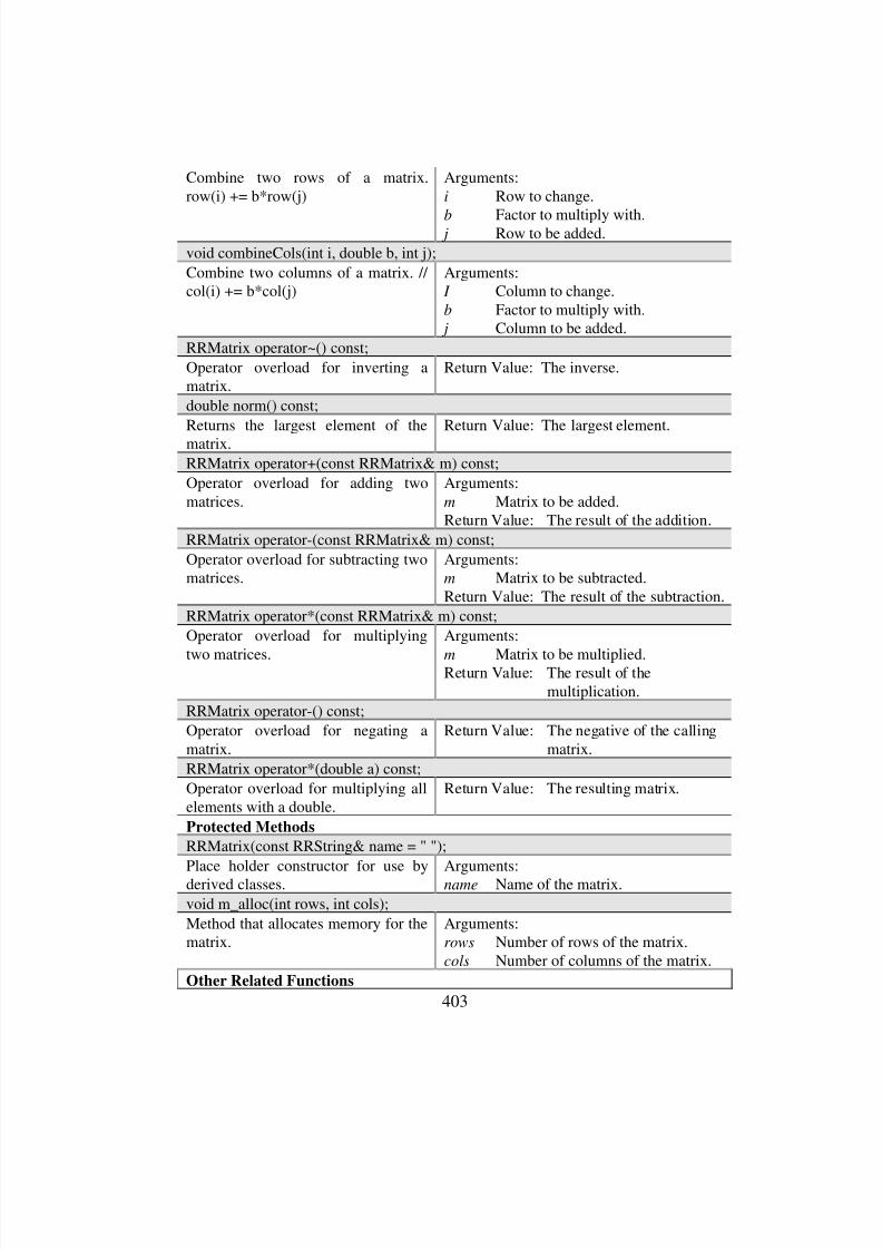
8/3/2019 Chetan Kapoor Dissertation
http://slidepdf.com/reader/full/chetan-kapoor-dissertation 424/612
403
Combine two rows of a matrix.row(i) += b*row(j)
Arguments:
i Row to change.
b Factor to multiply with. j Row to be added.
void combineCols(int i, double b, int j);
Combine two columns of a matrix. // col(i) += b*col(j)
Arguments: I Column to change.
b Factor to multiply with. j Column to be added.
RRMatrix operator~() const;
Operator overload for inverting amatrix.
Return Value: The inverse.
double norm() const;
Returns the largest element of the
matrix.
Return Value: The largest element.
RRMatrix operator+(const RRMatrix& m) const;
Operator overload for adding twomatrices.
Arguments:
m Matrix to be added.Return Value: The result of the addition.
RRMatrix operator-(const RRMatrix& m) const;
Operator overload for subtracting twomatrices.
Arguments:m Matrix to be subtracted.Return Value: The result of the subtraction.
RRMatrix operator*(const RRMatrix& m) const;
Operator overload for multiplying
two matrices.
Arguments:
m Matrix to be multiplied.Return Value: The result of the
multiplication.
RRMatrix operator-() const;
Operator overload for negating amatrix.
Return Value: The negative of the callingmatrix.
RRMatrix operator*(double a) const;
Operator overload for multiplying allelements with a double.
Return Value: The resulting matrix.
Protected Methods
RRMatrix(const RRString& name = " ");
Place holder constructor for use byderived classes.
Arguments:name Name of the matrix.
void m_alloc(int rows, int cols);
Method that allocates memory for thematrix.
Arguments:rows Number of rows of the matrix.
cols Number of columns of the matrix.
Other Related Functions
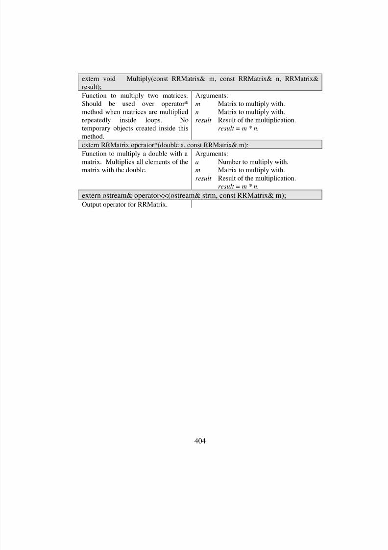
8/3/2019 Chetan Kapoor Dissertation
http://slidepdf.com/reader/full/chetan-kapoor-dissertation 425/612
404
extern void Multiply(const RRMatrix& m, const RRMatrix& n, RRMatrix&result);
Function to multiply two matrices.Should be used over operator*method when matrices are multipliedrepeatedly inside loops. Notemporary objects created inside thismethod.
Arguments:m Matrix to multiply with.n Matrix to multiply with.
result Result of the multiplication.result = m * n.
extern RRMatrix operator*(double a, const RRMatrix& m);
Function to multiply a double with amatrix. Multiplies all elements of thematrix with the double.
Arguments:
a Number to multiply with.m Matrix to multiply with.
result Result of the multiplication.result = m * n.
extern ostream& operator<<(ostream& strm, const RRMatrix& m);Output operator for RRMatrix.
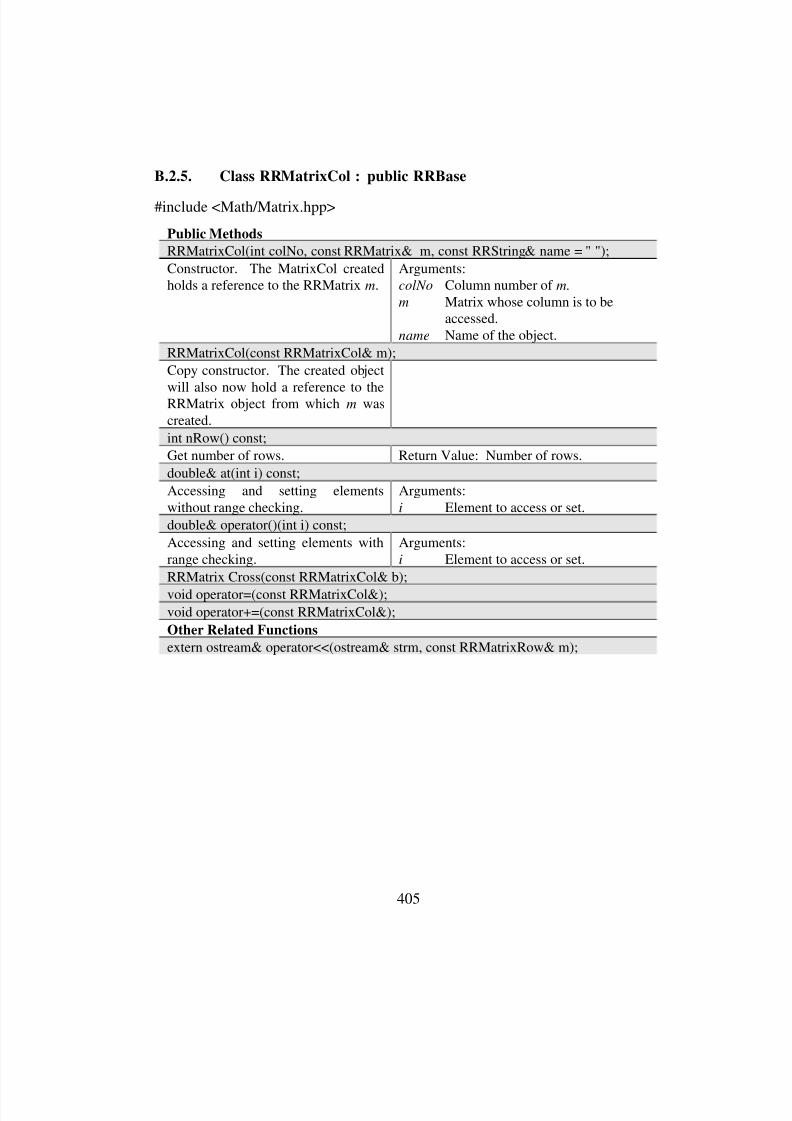
8/3/2019 Chetan Kapoor Dissertation
http://slidepdf.com/reader/full/chetan-kapoor-dissertation 426/612
405
B.2.5. Class RRMatrixCol : public RRBase
#include <Math/Matrix.hpp>
Public Methods
RRMatrixCol(int colNo, const RRMatrix& m, const RRString& name = " ");
Constructor. The MatrixCol createdholds a reference to the RRMatrix m.
Arguments:colNo Column number of m.
m Matrix whose column is to beaccessed.
name Name of the object.
RRMatrixCol(const RRMatrixCol& m);
Copy constructor. The created object
will also now hold a reference to theRRMatrix object from which m wascreated.
int nRow() const;
Get number of rows. Return Value: Number of rows.
double& at(int i) const;
Accessing and setting elementswithout range checking.
Arguments:
i Element to access or set.
double& operator()(int i) const;
Accessing and setting elements withrange checking.
Arguments:
i Element to access or set.
RRMatrix Cross(const RRMatrixCol& b);
void operator=(const RRMatrixCol&);
void operator+=(const RRMatrixCol&);
Other Related Functions
extern ostream& operator<<(ostream& strm, const RRMatrixRow& m);
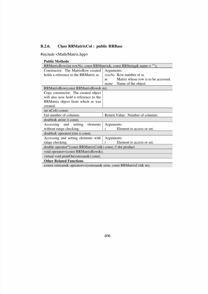
8/3/2019 Chetan Kapoor Dissertation
http://slidepdf.com/reader/full/chetan-kapoor-dissertation 427/612
406
B.2.6. Class RRMatrixCol : public RRBase
#include <Math/Matrix.hpp>
Public Methods
RRMatrixRow(int rowNo, const RRMatrix&, const RRString& name = "");
Constructor. The MatrixRow createdholds a reference to the RRMatrix m.
Arguments:rowNo Row number of m.
m Matrix whose row is to be accessed.name Name of the object.
RRMatrixRow(const RRMatrixRow& m);
Copy constructor. The created objectwill also now hold a reference to the
RRMatrix object from which m wascreated.
int nCol() const;
Get number of columns. Return Value: Number of columns.
double& at(int i) const;
Accessing and setting elementswithout range checking.
Arguments:i Element to access or set.
double& operator()(int i) const;
Accessing and setting elements withrange checking.
Arguments:i Element to access or set.
double operator^(const RRMatrixCol&) const; // dot product
void operator=(const RRMatrixRow&);
virtual void printOn(ostream&) const;
Other Related Functions
extern ostream& operator<<(ostream& strm, const RRMatrixCol& m);
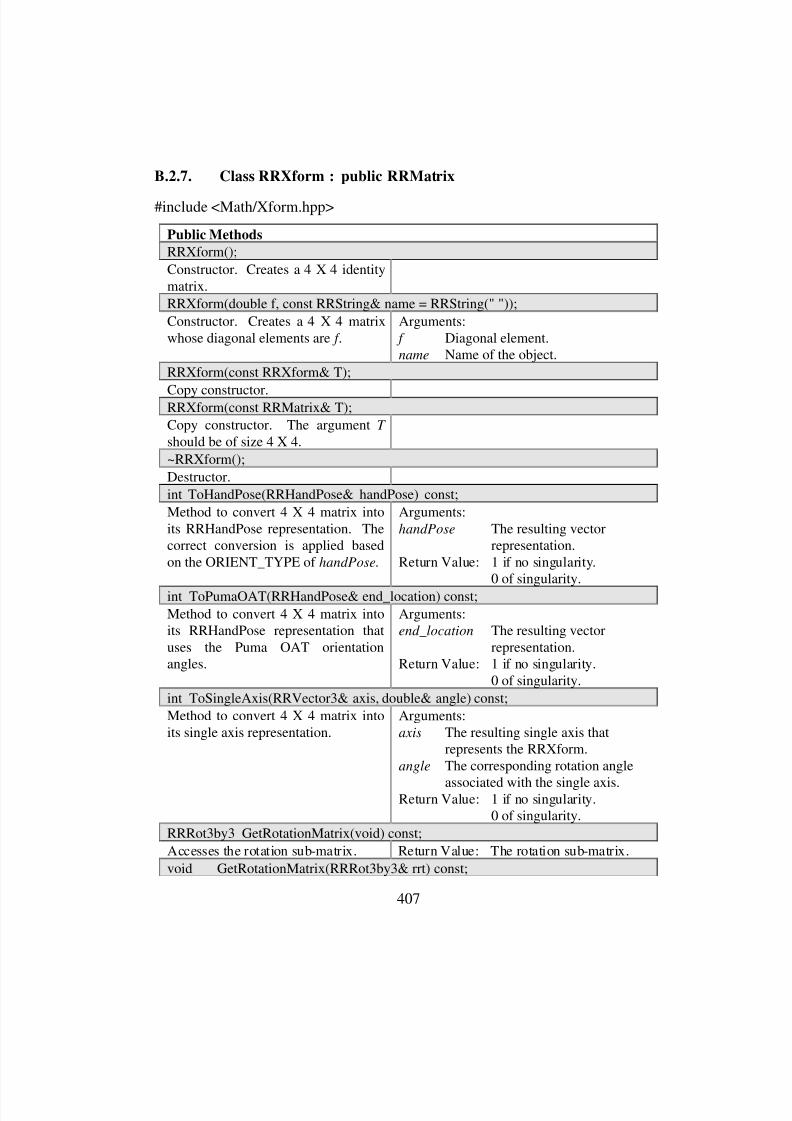
8/3/2019 Chetan Kapoor Dissertation
http://slidepdf.com/reader/full/chetan-kapoor-dissertation 428/612
407
B.2.7. Class RRXform : public RRMatrix
#include <Math/Xform.hpp>
Public Methods
RRXform();
Constructor. Creates a 4 X 4 identitymatrix.
RRXform(double f, const RRString& name = RRString(" "));
Constructor. Creates a 4 X 4 matrixwhose diagonal elements are f .
Arguments:
f Diagonal element.name Name of the object.
RRXform(const RRXform& T);
Copy constructor.RRXform(const RRMatrix& T);
Copy constructor. The argument T
should be of size 4 X 4.
~RRXform();
Destructor.
int ToHandPose(RRHandPose& handPose) const;
Method to convert 4 X 4 matrix intoits RRHandPose representation. Thecorrect conversion is applied basedon the ORIENT_TYPE of handPose.
Arguments:
handPose The resulting vectorrepresentation.
Return Value: 1 if no singularity.0 of singularity.
int ToPumaOAT(RRHandPose& end_location) const;
Method to convert 4 X 4 matrix intoits RRHandPose representation thatuses the Puma OAT orientationangles.
Arguments:end_location The resulting vector
representation.Return Value: 1 if no singularity.
0 of singularity.
int ToSingleAxis(RRVector3& axis, double& angle) const;
Method to convert 4 X 4 matrix intoits single axis representation.
Arguments:
axis The resulting single axis thatrepresents the RRXform.
angle The corresponding rotation angle
associated with the single axis.Return Value: 1 if no singularity.
0 of singularity.
RRRot3by3 GetRotationMatrix(void) const;
Accesses the rotation sub-matrix. Return Value: The rotation sub-matrix.
void GetRotationMatrix(RRRot3by3& rrt) const;
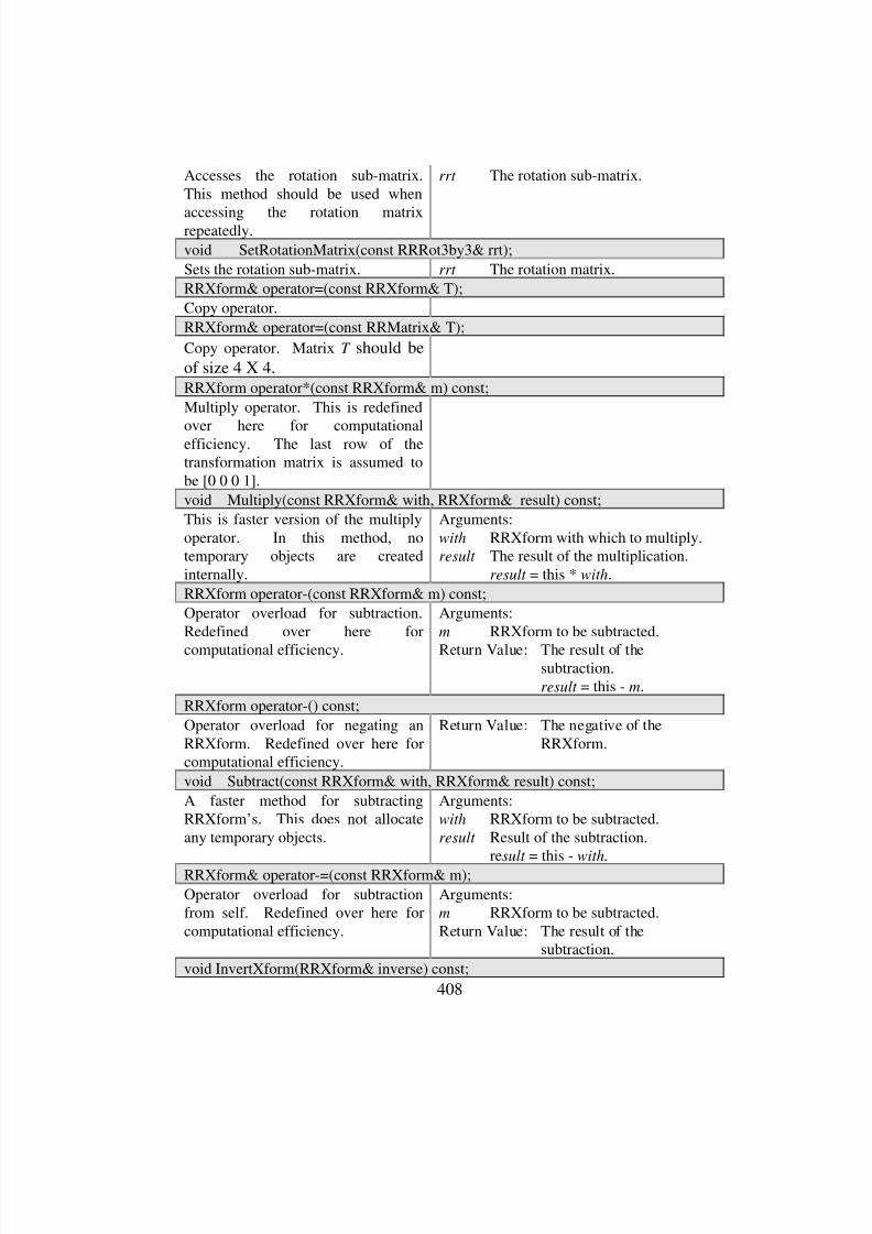
8/3/2019 Chetan Kapoor Dissertation
http://slidepdf.com/reader/full/chetan-kapoor-dissertation 429/612
408
Accesses the rotation sub-matrix.This method should be used when
accessing the rotation matrixrepeatedly.
rrt The rotation sub-matrix.
void SetRotationMatrix(const RRRot3by3& rrt);
Sets the rotation sub-matrix. rrt The rotation matrix.
RRXform& operator=(const RRXform& T);
Copy operator.
RRXform& operator=(const RRMatrix& T);
Copy operator. Matrix T should beof size 4 X 4.RRXform operator*(const RRXform& m) const;
Multiply operator. This is redefined
over here for computationalefficiency. The last row of thetransformation matrix is assumed tobe [0 0 0 1].
void Multiply(const RRXform& with, RRXform& result) const;
This is faster version of the multiplyoperator. In this method, notemporary objects are createdinternally.
Arguments:
with RRXform with which to multiply.result The result of the multiplication.
result = this * with.
RRXform operator-(const RRXform& m) const;
Operator overload for subtraction.Redefined over here for
computational efficiency.
Arguments:
m RRXform to be subtracted.
Return Value: The result of thesubtraction.
result = this - m.
RRXform operator-() const;
Operator overload for negating anRRXform. Redefined over here forcomputational efficiency.
Return Value: The negative of theRRXform.
void Subtract(const RRXform& with, RRXform& result) const;
A faster method for subtractingRRXform’s. This does not allocateany temporary objects.
Arguments:with RRXform to be subtracted.
result Result of the subtraction.result = this - with.
RRXform& operator-=(const RRXform& m);
Operator overload for subtractionfrom self. Redefined over here forcomputational efficiency.
Arguments:m RRXform to be subtracted.Return Value: The result of the
subtraction.
void InvertXform(RRXform& inverse) const;

8/3/2019 Chetan Kapoor Dissertation
http://slidepdf.com/reader/full/chetan-kapoor-dissertation 430/612
409
Method for inversion of a 4 X 4transformation matrix. This is more
efficient than the Inverse methoddefined in the RRMatrix class. Thismethod should be preferred whencalled inside loops.
Arguments:
inverse The Inverse.
RRXform InvertXform(void) const;
Method for inversion of a 4 X 4transformation matrix. This is moreefficient than the Inverse methoddefined in the RRMatrix class. Thismethod allocates a temporary objectinternally and hence is slower.
Return Value: The Inverse.
Protected Methods
void m_alloc(int nrow, int ncol);Method for allocating memory. Thisis redefined over here because theRRMatrix m_alloc method allocatesmemory on the heap and this methodallocates on the stack.
Arguments:nrow Number of rows = 4.
ncol Number of columns = 4.
int toEulerXYZ(RRHandPose& endLocation) const;
Method for converting a 4 X 4homogenous transformation matrixinto an RRHandPose whoseorientation type is Euler XYZ.
Arguments:
endLocation The converted RRXform.Return Value 1 if not singular.
0 if singular.
toEulerZYZ(RRHandPose& endLocation) const;Method for converting a 4 X 4homogenous transformation matrixinto an RRHandPose whoseorientation type is Euler ZYZ.
Arguments:
endLocation The converted RRXform.Return Value 1 if not singular.
0 if singular.
int toRPY(RRHandPose& endLocation) const;
Method for converting a 4 X 4homogenous transformation matrixinto an RRHandPose whoseorientation type is Fixed XYZ.
Arguments:
endLocation The converted RRXform.Return Value 1 if not singular.
0 if singular.

8/3/2019 Chetan Kapoor Dissertation
http://slidepdf.com/reader/full/chetan-kapoor-dissertation 431/612
410
B.2.8. Class RRRot3by3 : public RRMatrix
#include <Math/Rot3by3.hpp>
Public Methods
RRRot3by3();
Constructor. Creates a 3 X 3 matrix.
RRRot3by3(double f, const RRString& name = RRString(" "));
Constructor. Creates a 3 X 3 matrixwhose diagonal elements are f .
Arguments: f Diagonal element.
name Name of the object.
RRRot3by3(const RRRot3by3& T);
Copy constructor. Copies all the
elements of T into the createdmatrix.RRRot3by3(const RRMatrix& T);
Copy constructor. Copies all the
elements of T into the createdmatrix. Matrix T should be of size
3 X 3.~RRRot3by3();
Destructor.
void ToPumaOAT(RRVector3& endLocation) const;
Converts the 3 X 3 rotation matrix
into the orientation representationsimilar to the one used on Pumarobots.
Arguments:
endLocation The converted form.
void ToEulerXYZ(RRVector3& endLocation) const;
Converts the 3 X 3 rotation matrixinto its Euler XYZ representation.
Arguments:
endLocation The converted form.
void ToEulerZYZ(RRVector3& endLocation) const;
Converts the 3 X 3 rotation matrixinto its Euler ZYZ representation.
Arguments:
endLocation The converted form.
void ToRPY(RRVector3& endLocation) const;
Converts the 3 X 3 rotation matrixinto its Fixed XYZ representation.
Arguments:
endLocation The converted form.
RRVector3 ToRPY(void) const;
Converts the 3 X 3 rotation matrixinto its Fixed XYZ representation andreturns the result.
Return Value: The converted form.
RRRot3by3& operator=(const RRRot3by3& T);

8/3/2019 Chetan Kapoor Dissertation
http://slidepdf.com/reader/full/chetan-kapoor-dissertation 432/612
411
Copy operator. Copies all elements. Arguments:
T Object to be copied.
RRRot3by3& operator=(const RRMatrix& T);Copy operator. The argument T
should be of size 3 X 3.Arguments:T Object to be copied.
RRRot3by3 operator*(const RRRot3by3& m) const;
Multiplication operator. Arguments:m Object to be multiplied with.
RRRot3by3 operator*(const RRMatrix& m) const;
Multiplication operator. Matrix m
should be of size 3 X 3.Arguments:m Object to be multiplied with.
void Multiply(const RRRot3by3& with, RRRot3by3& result) const;
Multiplication method. Notemporaries created in this methodand hence is faster.
Arguments:
with Object to be multiplied with.result Result of the multiplication.
result = this * with.
void Multiply(const RRMatrix& with, RRRot3by3& result) const;
Multiplication method. Notemporaries created in this methodand hence is faster. Matrix with
should be of size 3 X 3.
Arguments:
with Object to be multiplied with.result Result of the multiplication.
result = this * with.
void Multiply(const RRVector3& with, RRVector3& result) const;
Multiply an RRRot3by3 with anRRVector3. No temporaries createdin this method and hence is faster.
Arguments:
with Object to be multiplied with.result Result of the multiplication.
result = this * with.RRRot3by3 t(void) const;
void Multiply(const RRVector3& with, RRVector3& result) const;
Multiply an RRRot3by3 with a tRRVector3. No temporaries createdin this method and hence is faster.
Arguments:
with Object to be multiplied with.result Result of the multiplication.
result = this * with.
void t(RRRot3by3& transpose) const;
Transpose method redefined forefficiency.
Arguments:
transpose Result of the transposeoperation.
void MultiplyWithTranspose(RRRot3by3& rrt) const;
Multiplies an RRRot3by3 with itstranspose. This method is redefinedfor efficiency.
Arguments:rrt Result of the multiplication.
void SetRotationAngles(const RRVector3D& axis, double theta, int angleType= 1 /* degrees */ );

8/3/2019 Chetan Kapoor Dissertation
http://slidepdf.com/reader/full/chetan-kapoor-dissertation 433/612
412
This method sets the element of thematrix based on the rotation axis and
the angle of rotation. For example, if a rotation matrix has to be createdthat rotates about the ‘X’ axis by 45.0degrees, then the arguments to thismethod will be:RRVector3 axis(1.0, 0.0, 0.0);double theta = 45.0;
Arguments:
axis Axis about which to rotate.
theta Angle amount to rotate. AngleType 1 is degrees.
0 is radians.
RRRot3by3 operator-(const RRRot3by3& m) const;
Subtraction operator redefined forRRRot3by3 for efficiency.
void Subtract(const RRRot3by3& with, RRRot3by3& result) const;
Subtraction method. This is a faster
version of the above method as notemporaries are created in thismethod.
Arguments:
with Matrix to be subtracted.result Result of the subtraction.
result = this - with.
RRVector3 operator*(const RRVector3& ) const;
Multiply operator. Multiplies with anRRVector3.
RRRot3by3 operator-() const;
Negative operator redefined forefficiency.
RRRot3by3& operator-=(const RRRot3by3& m);
Self subtraction operator redefined
for RRRot3by3 for efficiency.Protected Methods
void m_alloc(int nrow, int ncol);
Method for allocating memory. Thisis redefined over here because theRRMatrix m_alloc method allocatesmemory on the heap and this methodallocates on the stack.
Arguments:nrow Number of rows = 3.
ncol Number of columns = 3.

8/3/2019 Chetan Kapoor Dissertation
http://slidepdf.com/reader/full/chetan-kapoor-dissertation 434/612
413
B.2.9. Class RRTensor : public RRMatrix
#include <Math/Tensor.hpp>
Friend Member Functions
friend ostream& operator<<(ostream& strm, const RRTensor& t);
Output operator.
Public Methods
RRTensor(int nm = 1, RRMatrix* mp = 0, const RRString& name = "");
Constructor. Creates a tensor out of an array of matrices. The size of matrices in the mp array should all besame.
Arguments:
nm Number of matrices in mp.mp RRMatrix array.
name Name of the object.
RRTensor(int nm = 1, int Nrow = 1, int Ncol = 1, const RRString name = "");Constructor. Creates a tensor of size
nm X Nrow X Ncol and initializes allelements to 0.0.
Arguments:
nm Number of matrices in mp. Nrow Number of rows in a matrix.
Ncol Number of columns in a matrix.name Name of the object.
RRTensor(const RRTensor& t);
Copy constructor. Creates a tensorand copies all the elements of t into it.
~RRTensor();
Destructor. Deallocates memory.
int nMatrix() const;
Gets the number of rows in thematrices that comprise the tensor.
Return Value: The number of rows.
int nRow() const;
Gets the number of matrices in thetensor.
Return Value: The number of matrices.
int nCol() const;
Gets the number of columns in thematrices that comprise the tensor.
Return Value: The number of columns.
RRTensor& operator=(const RRTensor&);
Copy operator. Copies all theelements.
double& at(int i, int j, int k) const;Accesses or sets the i, j, k , element of the tensor. No range checking isperformed.
Arguments:
i j, k The element to access or set.Return Value: The i, j, k element.
double& operator()(int i, int j, int k) const;
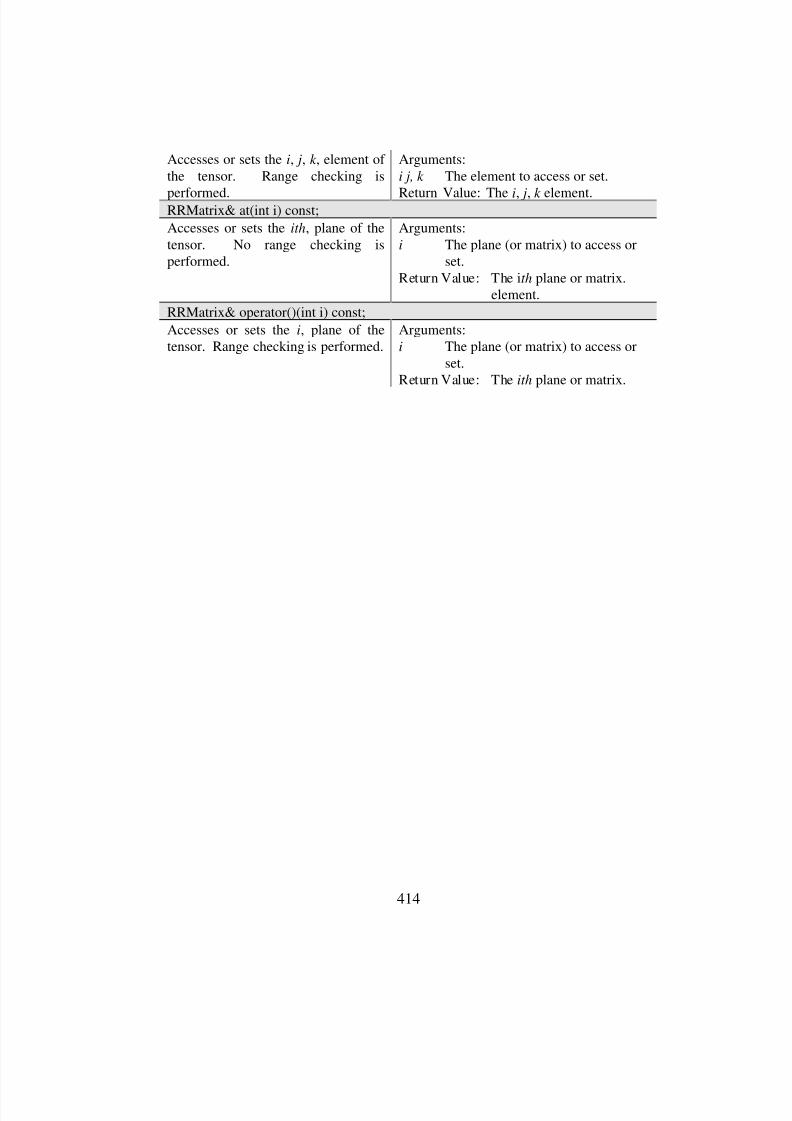
8/3/2019 Chetan Kapoor Dissertation
http://slidepdf.com/reader/full/chetan-kapoor-dissertation 435/612
414
Accesses or sets the i, j, k , element of the tensor. Range checking is
performed.
Arguments:
i j, k The element to access or set.
Return Value: The i, j, k element.RRMatrix& at(int i) const;
Accesses or sets the ith, plane of thetensor. No range checking isperformed.
Arguments:
i The plane (or matrix) to access orset.
Return Value: The ith plane or matrix.element.
RRMatrix& operator()(int i) const;
Accesses or sets the i, plane of thetensor. Range checking is performed.
Arguments:i The plane (or matrix) to access or
set.Return Value: The ith plane or matrix.

8/3/2019 Chetan Kapoor Dissertation
http://slidepdf.com/reader/full/chetan-kapoor-dissertation 436/612
415
B.3. Robot Data Abstractions
B.3.1. class RRRobotData : public RRBase
Abstract Data Type
#include <RobotData/RobotData.hpp>
Public Methods
RRRobotData(const RRString& name = RRString(" "));
Constructor for Abstract class. Arguments:
name Name of the object.
RRRobotData(const RRRobotData&);
Copy constructor.
virtual ~RRRobotData();
Destructor
Protected Methods
void open(char* filename, ifstream& inFile);
Opens a file and returns the inputstream to the calling method.
Arguments:
filename File to open.inFile The input stream associated
with filename.
virtual void parseComments(ifstream& file, const char marker);
Move the file pointer till it encounters
a valid field. A comment field isspecified by marker . Every time the
marker character is encountered, theremaining line is ignored ascomments.
Arguments:
file File to parse.marker A character that specifies the start
of comments.
virtual int GetNoofEntries(ifstream& file, const char marker);
Method to compute the total numberof valid entries in the file.
Arguments: file File to parse.
marker A character that specifies the startof comments.
Return Value: The number of valid entriesin the file.
RRRobotData& operator=(const RRRobotData&);
Copy operator.
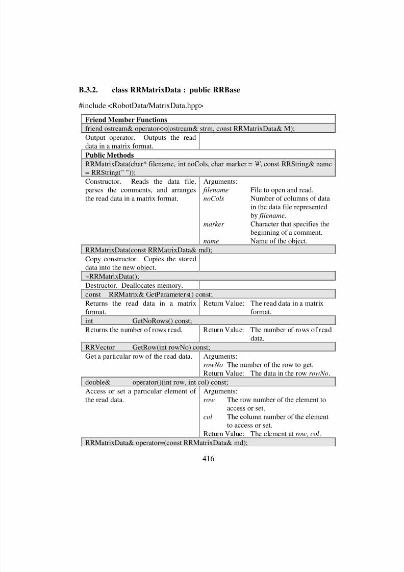
8/3/2019 Chetan Kapoor Dissertation
http://slidepdf.com/reader/full/chetan-kapoor-dissertation 437/612
416
B.3.2. class RRMatrixData : public RRBase
#include <RobotData/MatrixData.hpp>
Friend Member Functions
friend ostream& operator<<(ostream& strm, const RRMatrixData& M);
Output operator. Outputs the readdata in a matrix format.
Public Methods
RRMatrixData(char* filename, int noCols, char marker = ’#’, const RRString& name= RRString(" "));
Constructor. Reads the data file,parses the comments, and arranges
the read data in a matrix format.
Arguments:
filename File to open and read.
noCols Number of columns of datain the data file representedby filename.
marker Character that specifies thebeginning of a comment.
name Name of the object.
RRMatrixData(const RRMatrixData& md);
Copy constructor. Copies the storeddata into the new object.
~RRMatrixData();
Destructor. Deallocates memory.
const RRMatrix& GetParameters() const;
Returns the read data in a matrixformat.
Return Value: The read data in a matrixformat.
int GetNoRows() const;
Returns the number of rows read. Return Value: The number of rows of readdata.
RRVector GetRow(int rowNo) const;
Get a particular row of the read data. Arguments:rowNo The number of the row to get.Return Value: The data in the row rowNo.
double& operator()(int row, int col) const;
Access or set a particular element of
the read data.
Arguments:
row The row number of the element toaccess or set.
col The column number of the elementto access or set.
Return Value: The element at row, col.
RRMatrixData& operator=(const RRMatrixData& md);
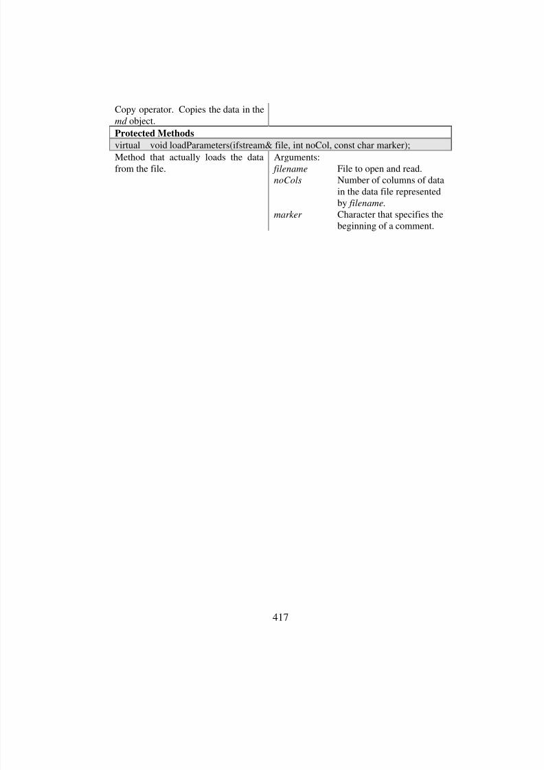
8/3/2019 Chetan Kapoor Dissertation
http://slidepdf.com/reader/full/chetan-kapoor-dissertation 438/612
417
Copy operator. Copies the data in the
md object.
Protected Methodsvirtual void loadParameters(ifstream& file, int noCol, const char marker);
Method that actually loads the datafrom the file.
Arguments:
filename File to open and read.noCols Number of columns of data
in the data file representedby filename.
marker Character that specifies thebeginning of a comment.
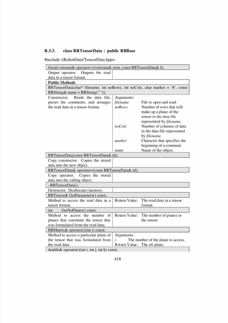
8/3/2019 Chetan Kapoor Dissertation
http://slidepdf.com/reader/full/chetan-kapoor-dissertation 439/612
418
B.3.3. class RRTensorData : public RRBase
#include <RobotData/TensorData.hpp>
friend ostream& operator<<(ostream& strm, const RRTensorData& I);
Output operator. Outputs the readdata in a tensor format.
Public Methods
RRTensorData(char* filename, int noRows, int noCols, char marker = ’#’, constRRString& name = RRString(" "));
Constructor. Reads the data file,parses the comments, and arrangesthe read data in a tensor format.
Arguments: filename File to open and read.
noRows Number of rows that will
make up a plane of thetensor in the data filerepresented by filename.
noCols Number of columns of datain the data file representedby filename.
marker Character that specifies thebeginning of a comment.
name Name of the object.
RRTensorData(const RRTensorData& td);
Copy constructor. Copies the storeddata into the new object.
RRTensorData& operator=(const RRTensorData& td);Copy operator. Copies the storeddata into the calling object.
~RRTensorData();
Destructor. Deallocates memory.
RRTensor& GetParameters() const;
Method to access the read data in atensor format.
Return Value: The read data in a tensorformat.
int GetNoPlanes() const;
Method to access the number of planes that constitute the tensor that
was formulated from the read data.
Return Value: The number of planes inthe tensor.
RRMatrix& operator()(int i) const;
Method to access a particular plane of the tensor that was formulated fromthe read data.
Arguments:
i The number of the plane to access.Return Value: The ith plane.
double& operator()(int i, int j, int k) const;
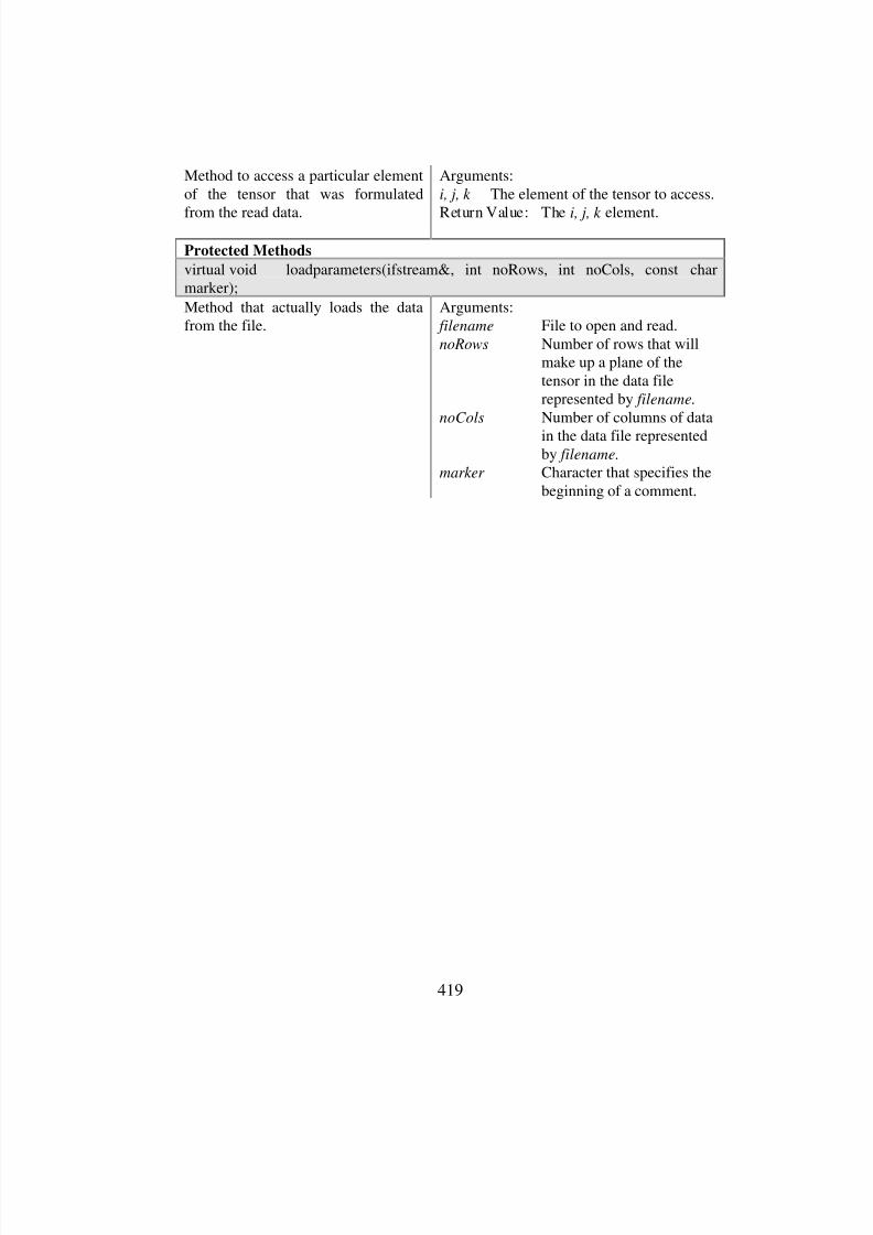
8/3/2019 Chetan Kapoor Dissertation
http://slidepdf.com/reader/full/chetan-kapoor-dissertation 440/612
419
Method to access a particular elementof the tensor that was formulated
from the read data.
Arguments:
i, j, k The element of the tensor to access.
Return Value: The i, j, k element.
Protected Methods
virtual void loadparameters(ifstream&, int noRows, int noCols, const charmarker);
Method that actually loads the datafrom the file.
Arguments: filename File to open and read.
noRows Number of rows that willmake up a plane of thetensor in the data filerepresented by filename.
noCols Number of columns of data
in the data file representedby filename.
marker Character that specifies thebeginning of a comment.
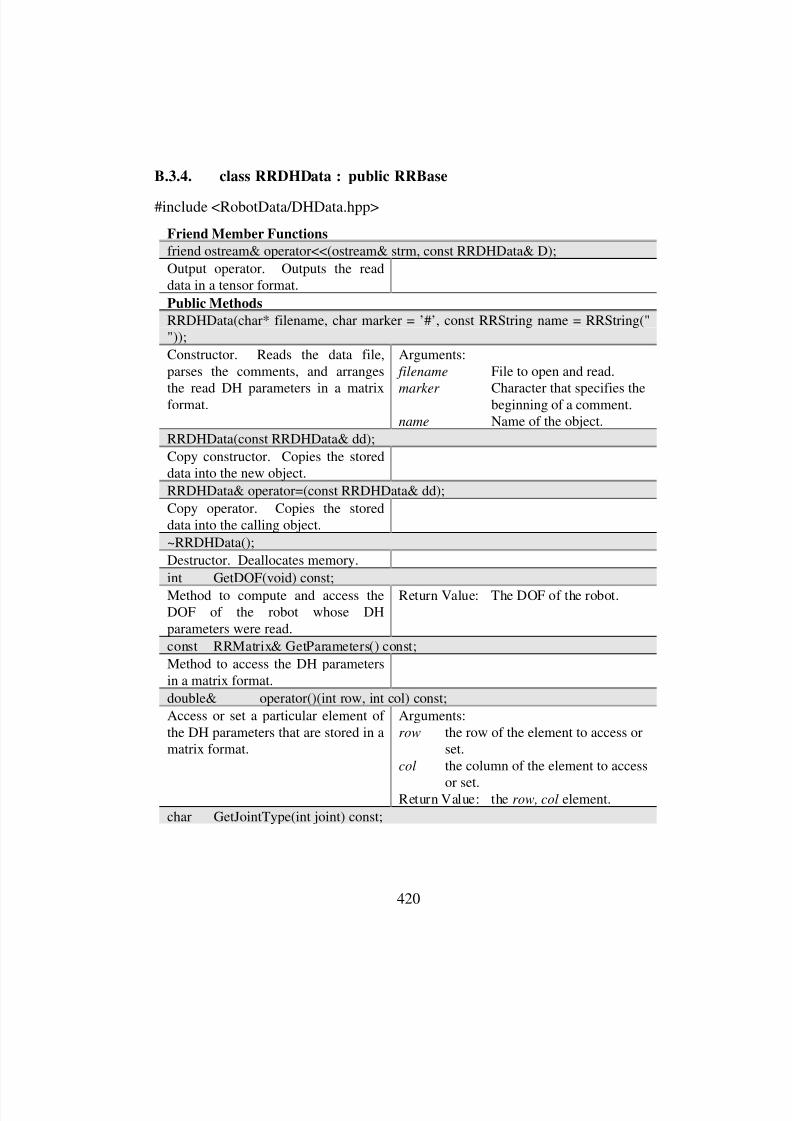
8/3/2019 Chetan Kapoor Dissertation
http://slidepdf.com/reader/full/chetan-kapoor-dissertation 441/612
420
B.3.4. class RRDHData : public RRBase
#include <RobotData/DHData.hpp>
Friend Member Functions
friend ostream& operator<<(ostream& strm, const RRDHData& D);
Output operator. Outputs the readdata in a tensor format.
Public Methods
RRDHData(char* filename, char marker = ’#’, const RRString name = RRString(""));
Constructor. Reads the data file,parses the comments, and arranges
the read DH parameters in a matrixformat.
Arguments:
filename File to open and read.
marker Character that specifies thebeginning of a comment.name Name of the object.
RRDHData(const RRDHData& dd);
Copy constructor. Copies the storeddata into the new object.
RRDHData& operator=(const RRDHData& dd);
Copy operator. Copies the storeddata into the calling object.
~RRDHData();
Destructor. Deallocates memory.
int GetDOF(void) const;
Method to compute and access theDOF of the robot whose DHparameters were read.
Return Value: The DOF of the robot.
const RRMatrix& GetParameters() const;
Method to access the DH parametersin a matrix format.
double& operator()(int row, int col) const;
Access or set a particular element of the DH parameters that are stored in amatrix format.
Arguments:
row the row of the element to access orset.
col the column of the element to access
or set.Return Value: the row, col element.
char GetJointType(int joint) const;

8/3/2019 Chetan Kapoor Dissertation
http://slidepdf.com/reader/full/chetan-kapoor-dissertation 442/612
421
Get the joint type of a particular joint. Arguments:
joint The joint number whose type is
desired.Return Value: ‘P’ if joint is prismatic.
‘R’ if joint is revolute.
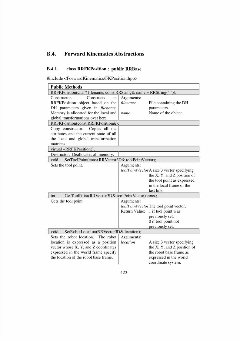
8/3/2019 Chetan Kapoor Dissertation
http://slidepdf.com/reader/full/chetan-kapoor-dissertation 443/612
422
B.4. Forward Kinematics Abstractions
B.4.1. class RRFKPosition : public RRBase
#include <ForwardKinematics/FKPosition.hpp>
Public Methods
RRFKPosition(char* filename, const RRString& name = RRString(" "));
Constructor. Constructs anRRFKPosition object based on theDH parameters given in filename.
Memory is allocated for the local and
global transformations over here.
Arguments:
filename File containing the DHparameters.
name Name of the object.
RRFKPosition(const RRFKPosition&);
Copy constructor. Copies all theattributes and the current state of allthe local and global transformationmatrices.
virtual ~RRFKPosition();
Destructor. Deallocates all memory.
void SetToolPoint(const RRVector3D& toolPointVector);
Sets the tool point. Arguments:toolPointVector A size 3 vector specifying
the X, Y, and Z position of
the tool point as expressedin the local frame of thelast link.
int GetToolPoint(RRVector3D& toolPointVector) const;
Gets the tool point. Arguments:
toolPointVector The tool point vector.Return Value: 1 if tool point was
previously set.0 if tool point notpreviously set.
void SetRobotLocation(RRVector3D& location);
Sets the robot location. The robotlocation is expressed as a positionvector whose X, Y, and Z coordinatesexpressed in the world frame specifythe location of the robot base frame.
Arguments:location A size 3 vector specifying
the X, Y, and Z position of the robot base frame asexpressed in the worldcoordinate system.
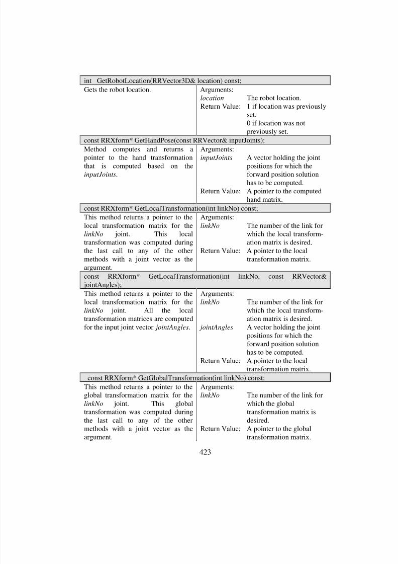
8/3/2019 Chetan Kapoor Dissertation
http://slidepdf.com/reader/full/chetan-kapoor-dissertation 444/612
423
int GetRobotLocation(RRVector3D& location) const;
Gets the robot location. Arguments:
location The robot location.Return Value: 1 if location was previously
set.0 if location was notpreviously set.
const RRXform* GetHandPose(const RRVector& inputJoints);
Method computes and returns apointer to the hand transformationthat is computed based on theinputJoints.
Arguments:inputJoints A vector holding the joint
positions for which theforward position solutionhas to be computed.
Return Value: A pointer to the computed
hand matrix.const RRXform* GetLocalTransformation(int linkNo) const;
This method returns a pointer to thelocal transformation matrix for thelinkNo joint. This localtransformation was computed duringthe last call to any of the othermethods with a joint vector as theargument.
Arguments:
linkNo The number of the link forwhich the local transform-ation matrix is desired.
Return Value: A pointer to the localtransformation matrix.
const RRXform* GetLocalTransformation(int linkNo, const RRVector& jointAngles);
This method returns a pointer to thelocal transformation matrix for the
linkNo joint. All the localtransformation matrices are computedfor the input joint vector jointAngles.
Arguments:linkNo The number of the link forwhich the local transform-ation matrix is desired.
jointAngles A vector holding the jointpositions for which theforward position solutionhas to be computed.
Return Value: A pointer to the localtransformation matrix.
const RRXform* GetGlobalTransformation(int linkNo) const;
This method returns a pointer to the
global transformation matrix for thelinkNo joint. This globaltransformation was computed duringthe last call to any of the othermethods with a joint vector as theargument.
Arguments:
linkNo The number of the link forwhich the globaltransformation matrix isdesired.
Return Value: A pointer to the globaltransformation matrix.

8/3/2019 Chetan Kapoor Dissertation
http://slidepdf.com/reader/full/chetan-kapoor-dissertation 445/612
424
const RRXform* GetGlobalTransformation(int linkNo, const RRVector& jointAngles);
This method returns a pointer to theglobal transformation matrix for thelinkNo joint. All the globaltransformation matrices are computedfor the input joint vector jointAngles.
Arguments:linkNo The number of the link for
which the globaltransformation matrix isdesired.
jointAngles A vector holding the jointpositions for which theforward position solutionhas to be computed.
Return Value: A pointer to the localtransformation matrix.
const RRXform* GetAllLocalTransformations() const;
This method returns a pointer to anarray of RRXform’s that holds thelocal transformation matrices (size =DOF of the robot). These localtransformations were computedduring the last call to any of the othermethods with a joint vector as theargument.
Return Value: A pointer to the localtransformation matricesarray.
const RRXform* GetAllLocalTransformations(const RRVector& jointAngles);
This method returns a pointer to thearray of local transformationmatrices. All the localtransformations matrices arecomputed for the input joint vector
jointAngles.
Arguments: jointAngles A vector holding the joint
positions for which theforward position solutionhas to be computed.
Return Value: A pointer to the array of local transformationmatrices.
const RRXform* GetAllGlobalTransformations() const;
This method returns a pointer to anarray of RRXform’s that holds theglobal transformation matrices (size =DOF of the robot). These globaltransformations were computed
during the last call to any of the othermethods with a joint vector as theargument.
Return Value: A pointer to the globaltransformation matricesarray.
const RRXform* GetAllGlobalTransformations(const RRVector& jointAngles);
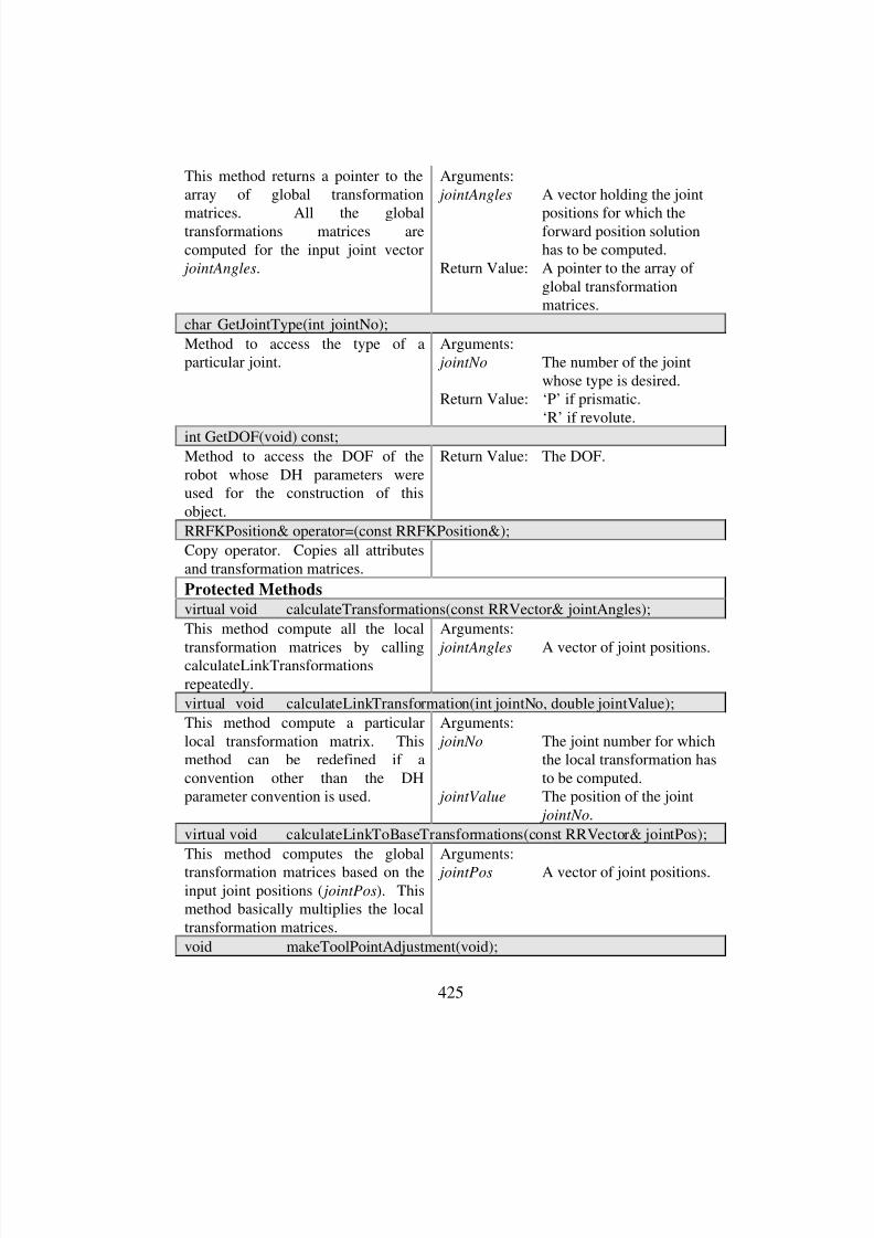
8/3/2019 Chetan Kapoor Dissertation
http://slidepdf.com/reader/full/chetan-kapoor-dissertation 446/612
425
This method returns a pointer to thearray of global transformation
matrices. All the globaltransformations matrices arecomputed for the input joint vector
jointAngles.
Arguments:
jointAngles A vector holding the joint
positions for which theforward position solutionhas to be computed.
Return Value: A pointer to the array of global transformationmatrices.
char GetJointType(int jointNo);
Method to access the type of aparticular joint.
Arguments: jointNo The number of the joint
whose type is desired.Return Value: ‘P’ if prismatic.
‘R’ if revolute.
int GetDOF(void) const;Method to access the DOF of therobot whose DH parameters wereused for the construction of thisobject.
Return Value: The DOF.
RRFKPosition& operator=(const RRFKPosition&);
Copy operator. Copies all attributesand transformation matrices.
Protected Methods
virtual void calculateTransformations(const RRVector& jointAngles);
This method compute all the local
transformation matrices by callingcalculateLinkTransformationsrepeatedly.
Arguments:
jointAngles A vector of joint positions.
virtual void calculateLinkTransformation(int jointNo, double jointValue);
This method compute a particularlocal transformation matrix. Thismethod can be redefined if aconvention other than the DHparameter convention is used.
Arguments:
joinNo The joint number for whichthe local transformation hasto be computed.
jointValue The position of the joint
jointNo.
virtual void calculateLinkToBaseTransformations(const RRVector& jointPos);
This method computes the global
transformation matrices based on theinput joint positions ( jointPos). Thismethod basically multiplies the localtransformation matrices.
Arguments:
jointPos A vector of joint positions.
void makeToolPointAdjustment(void);

8/3/2019 Chetan Kapoor Dissertation
http://slidepdf.com/reader/full/chetan-kapoor-dissertation 447/612
426
This method modifies the globaltransformation matrix of the last joint
based on the tool-point vector.void makeRobotLocationAdjustment(void);
This method modifies the localtransformation matrix of the first jointbased on the robot location vector.
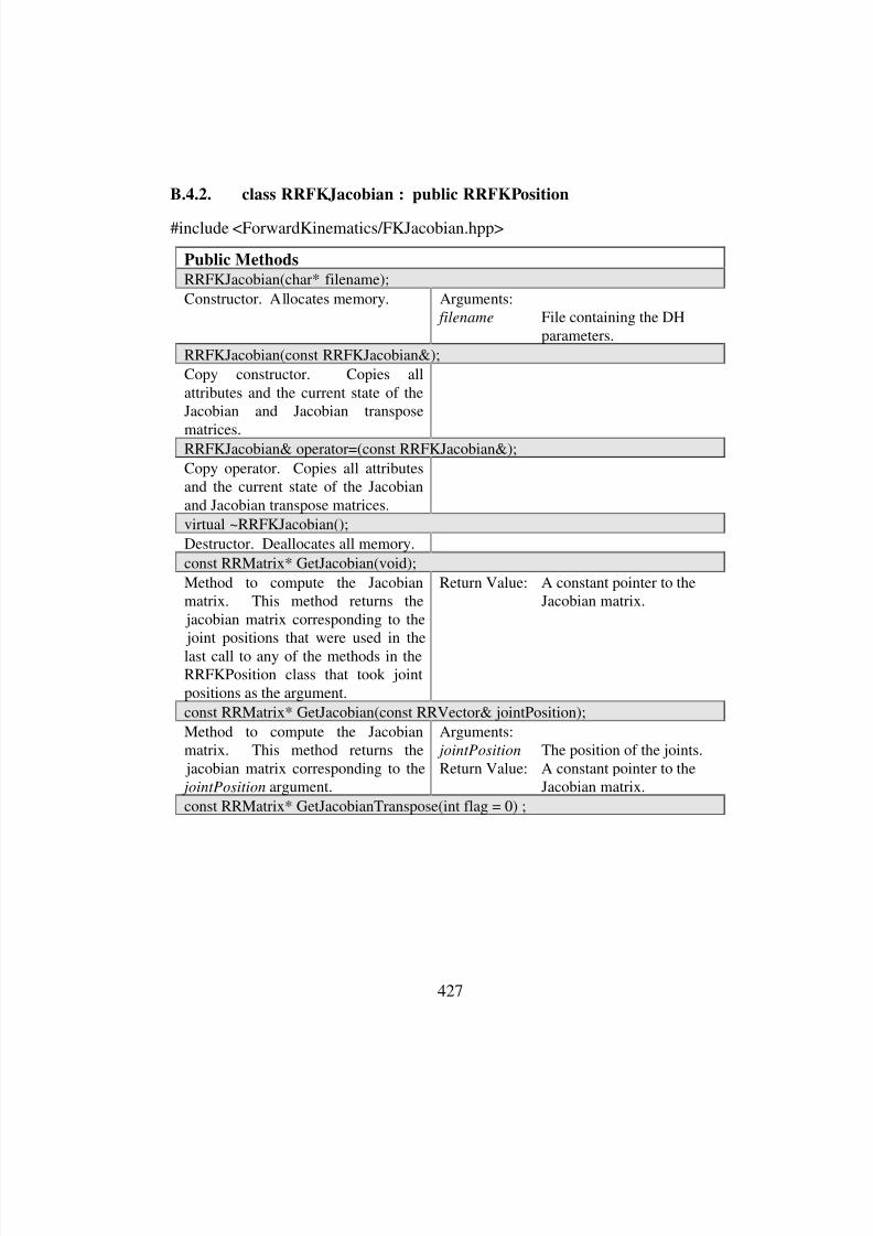
8/3/2019 Chetan Kapoor Dissertation
http://slidepdf.com/reader/full/chetan-kapoor-dissertation 448/612
427
B.4.2. class RRFKJacobian : public RRFKPosition
#include <ForwardKinematics/FKJacobian.hpp>
Public Methods
RRFKJacobian(char* filename);
Constructor. Allocates memory. Arguments: filename File containing the DH
parameters.
RRFKJacobian(const RRFKJacobian&);
Copy constructor. Copies allattributes and the current state of theJacobian and Jacobian transpose
matrices.RRFKJacobian& operator=(const RRFKJacobian&);
Copy operator. Copies all attributesand the current state of the Jacobianand Jacobian transpose matrices.
virtual ~RRFKJacobian();
Destructor. Deallocates all memory.
const RRMatrix* GetJacobian(void);
Method to compute the Jacobianmatrix. This method returns the jacobian matrix corresponding to the joint positions that were used in thelast call to any of the methods in theRRFKPosition class that took jointpositions as the argument.
Return Value: A constant pointer to theJacobian matrix.
const RRMatrix* GetJacobian(const RRVector& jointPosition);
Method to compute the Jacobianmatrix. This method returns the jacobian matrix corresponding to the jointPosition argument.
Arguments: jointPosition The position of the joints.Return Value: A constant pointer to the
Jacobian matrix.
const RRMatrix* GetJacobianTranspose(int flag = 0) ;
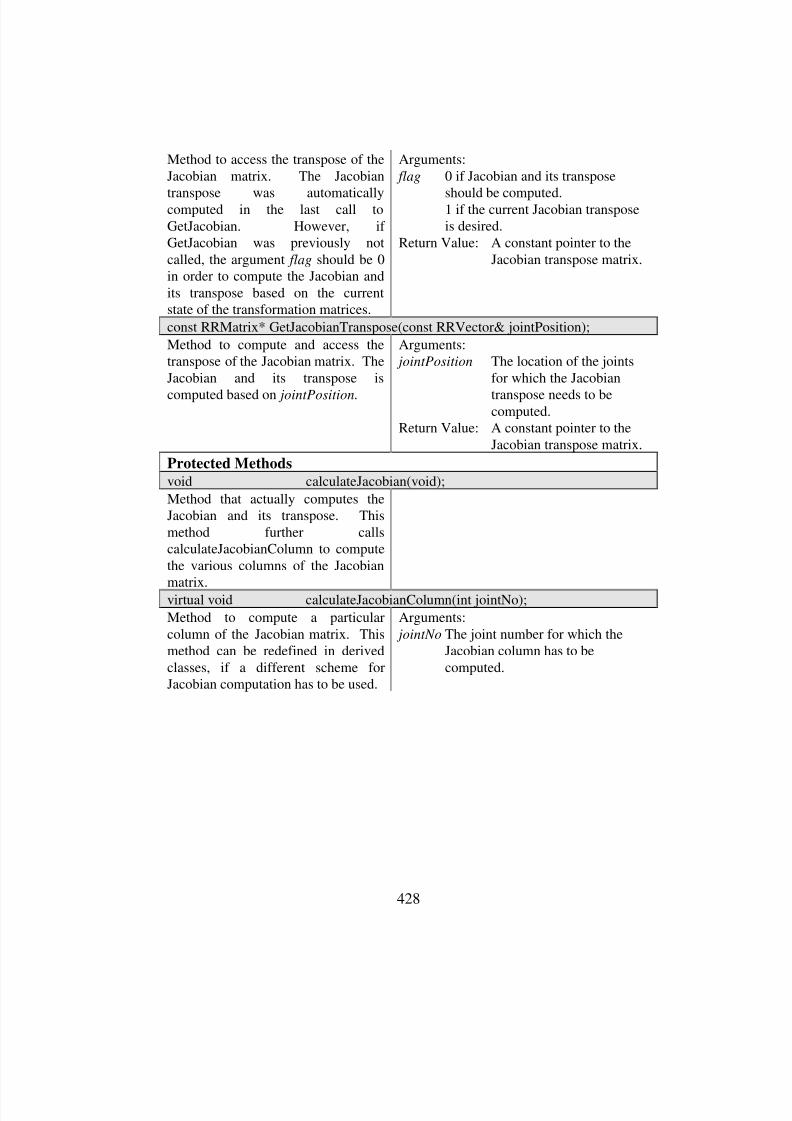
8/3/2019 Chetan Kapoor Dissertation
http://slidepdf.com/reader/full/chetan-kapoor-dissertation 449/612
428
Method to access the transpose of theJacobian matrix. The Jacobian
transpose was automaticallycomputed in the last call toGetJacobian. However, if GetJacobian was previously notcalled, the argument flag should be 0in order to compute the Jacobian andits transpose based on the currentstate of the transformation matrices.
Arguments:
flag 0 if Jacobian and its transpose
should be computed.1 if the current Jacobian transposeis desired.
Return Value: A constant pointer to theJacobian transpose matrix.
const RRMatrix* GetJacobianTranspose(const RRVector& jointPosition);
Method to compute and access thetranspose of the Jacobian matrix. TheJacobian and its transpose is
computed based on jointPosition.
Arguments: jointPosition The location of the joints
for which the Jacobian
transpose needs to becomputed.
Return Value: A constant pointer to theJacobian transpose matrix.
Protected Methods
void calculateJacobian(void);
Method that actually computes theJacobian and its transpose. Thismethod further callscalculateJacobianColumn to computethe various columns of the Jacobian
matrix.virtual void calculateJacobianColumn(int jointNo);
Method to compute a particularcolumn of the Jacobian matrix. Thismethod can be redefined in derivedclasses, if a different scheme forJacobian computation has to be used.
Arguments:
jointNo The joint number for which theJacobian column has to becomputed.
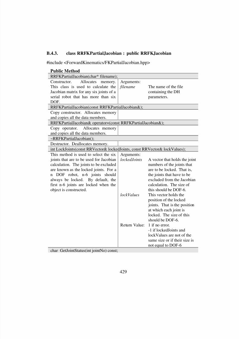
8/3/2019 Chetan Kapoor Dissertation
http://slidepdf.com/reader/full/chetan-kapoor-dissertation 450/612
429
B.4.3. class RRFKPartialJacobian : public RRFKJacobian
#include <ForwardKinematics/FKPartialJacobian.hpp>
Public Method
RRFKPartialJacobian(char* filename);
Constructor. Allocates memory.This class is used to calculate theJacobian matrix for any six joints of aserial robot that has more than sixDOF.
Arguments: filename The name of the file
containing the DHparameters.
RRFKPartialJacobian(const RRFKPartialJacobian&);
Copy constructor. Allocates memory
and copies all the data members.RRFKPartialJacobian& operator=(const RRFKPartialJacobian&);
Copy operator. Allocates memoryand copies all the data members.
~RRFKPartialJacobian();
Destructor. Deallocates memory.
int LockJoints(const RRVector& lockedJoints, const RRVector& lockValues);
This method is used to select the six joints that are to be used for Jacobiancalculation. The joints to be excludedare known as the locked joints. For an DOF robot, n-6 joints should
always be locked. By default, thefirst n-6 joints are locked when theobject is constructed.
Arguments:
lockedJoints A vector that holds the jointnumbers of the joints thatare to be locked. That is,the joints that have to be
excluded from the Jacobiancalculation. The size of this should be DOF-6.
lockValues This vector holds theposition of the locked joints. That is the positionat which each joint islocked. The size of thisshould be DOF-6.
Return Value: 1 if no error.-1 if lockedJoints andlockValues are not of thesame size or if their size isnot equal to DOF-6
char GetJointStatus(int jointNo) const;

8/3/2019 Chetan Kapoor Dissertation
http://slidepdf.com/reader/full/chetan-kapoor-dissertation 451/612
430
Method to access the status of a joint. Arguments:
jointNo The number of the joint
whose status is desired.Return Value: ’U’ if joint is unlocked.
’L’ if joint is locked.
const char* GetJointStatus(void) const;
Method to access the status of all the joints.
Return Value: A character array of sizeDOF that holds the statusof all joints. ’U’ if joint isunlocked. ’L’ if joint islocked.
double GetJointLockValue(int jointNo) const;
Method to access position at which a joint is locked.
Arguments: jointNo The joint for which the
locked value is desired.Return Value: A character array of size
DOF that holds the statusof all joints. ’U’ if joint isunlocked. ’L’ if joint islocked.
int GetLockedJoints(RRVector& lockedJoints, RRVector& lockedValues) const;
This method is used to access the joint numbers of the locked joints andvalues at which they are locked.
Arguments:lockedJoints A vector that holds the joint
numbers of the joints thatare locked. The size of thisshould be DOF-6.
lockValues This vector holds theposition of the locked joints. The size of thisshould be DOF-6.
Return Value: 1.
int SetLockedJoints(const RRVector& lockValues);
Set the locked values of the locked joints.
Arguments:
lockValues This vector holds theposition of the locked joints. That is the positionat which each joint is
locked. The size of thisshould be DOF-6.
Return Value: 1 if no error.0 if lockValues is not of size DOF-6.
const RRMatrix* GetPartialJacobian(void);
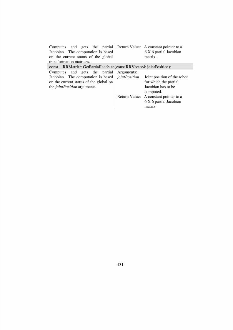
8/3/2019 Chetan Kapoor Dissertation
http://slidepdf.com/reader/full/chetan-kapoor-dissertation 452/612
431
Computes and gets the partialJacobian. The computation is based
on the current status of the globaltransformation matrices.
Return Value: A constant pointer to a6 X 6 partial Jacobian
matrix.
const RRMatrix* GetPartialJacobian(const RRVector& jointPosition);
Computes and gets the partialJacobian. The computation is basedon the current status of the global onthe jointPosition arguments.
Arguments: jointPosition Joint position of the robot
for which the partialJacobian has to becomputed.
Return Value: A constant pointer to a6 X 6 partial Jacobianmatrix.
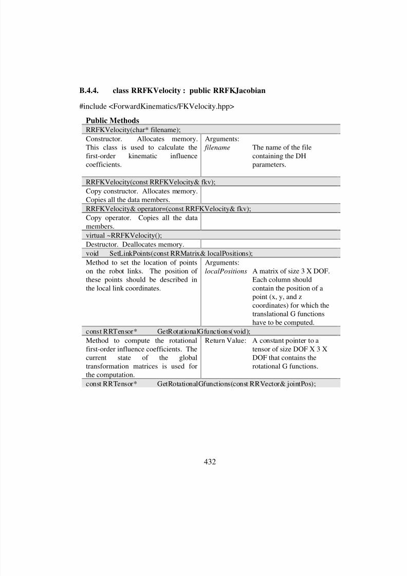
8/3/2019 Chetan Kapoor Dissertation
http://slidepdf.com/reader/full/chetan-kapoor-dissertation 453/612
432
B.4.4. class RRFKVelocity : public RRFKJacobian
#include <ForwardKinematics/FKVelocity.hpp>
Public Methods
RRFKVelocity(char* filename);
Constructor. Allocates memory.This class is used to calculate thefirst-order kinematic influencecoefficients.
Arguments: filename The name of the file
containing the DHparameters.
RRFKVelocity(const RRFKVelocity& fkv);
Copy constructor. Allocates memory.
Copies all the data members.RRFKVelocity& operator=(const RRFKVelocity& fkv);
Copy operator. Copies all the datamembers.
virtual ~RRFKVelocity();
Destructor. Deallocates memory.
void SetLinkPoints(const RRMatrix& localPositions);
Method to set the location of pointson the robot links. The position of these points should be described inthe local link coordinates.
Arguments:
localPositions A matrix of size 3 X DOF.Each column shouldcontain the position of apoint (x, y, and z
coordinates) for which thetranslational G functionshave to be computed.
const RRTensor* GetRotationalGfunctions(void);
Method to compute the rotationalfirst-order influence coefficients. Thecurrent state of the globaltransformation matrices is used forthe computation.
Return Value: A constant pointer to atensor of size DOF X 3 XDOF that contains therotational G functions.
const RRTensor* GetRotationalGfunctions(const RRVector& jointPos);
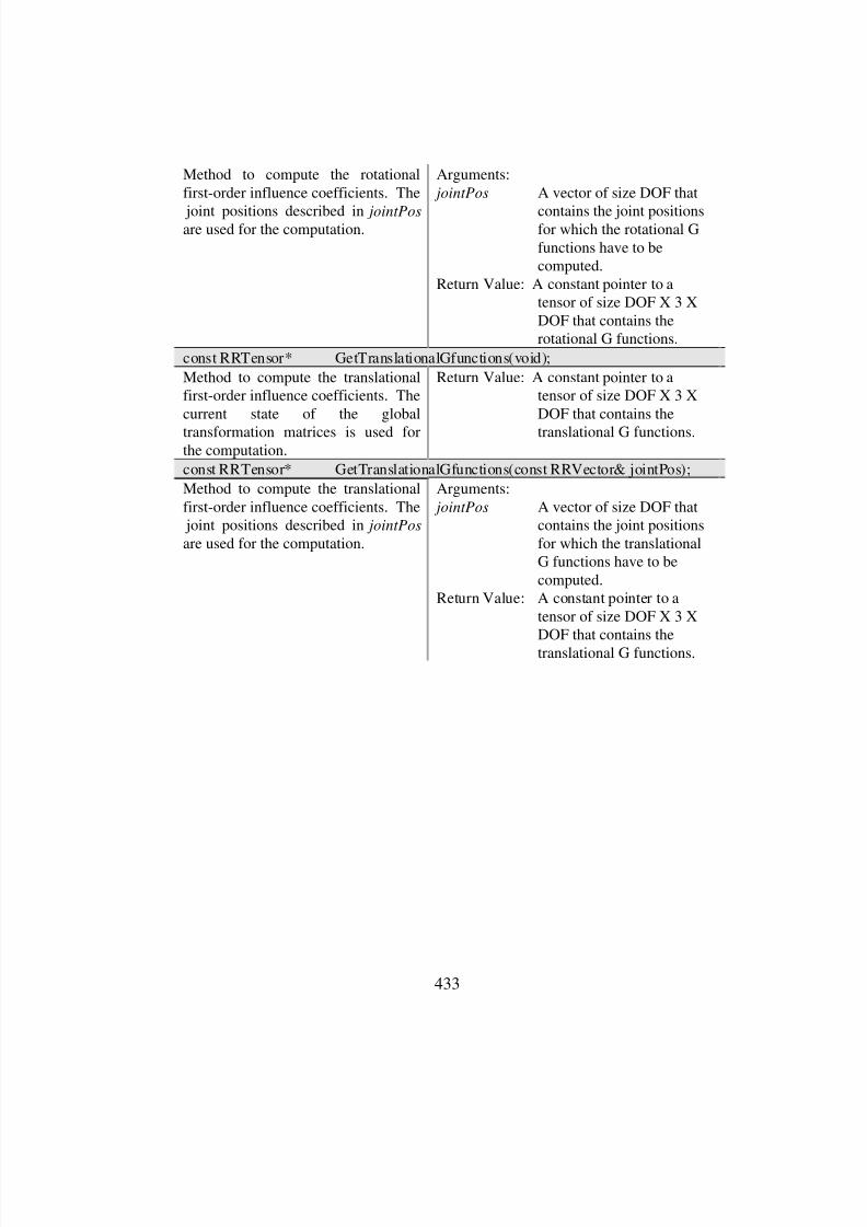
8/3/2019 Chetan Kapoor Dissertation
http://slidepdf.com/reader/full/chetan-kapoor-dissertation 454/612
433
Method to compute the rotationalfirst-order influence coefficients. The
joint positions described in jointPosare used for the computation.
Arguments:
jointPos A vector of size DOF that
contains the joint positionsfor which the rotational Gfunctions have to becomputed.
Return Value: A constant pointer to atensor of size DOF X 3 XDOF that contains therotational G functions.
const RRTensor* GetTranslationalGfunctions(void);
Method to compute the translationalfirst-order influence coefficients. Thecurrent state of the global
transformation matrices is used forthe computation.
Return Value: A constant pointer to atensor of size DOF X 3 XDOF that contains the
translational G functions.
const RRTensor* GetTranslationalGfunctions(const RRVector& jointPos);
Method to compute the translationalfirst-order influence coefficients. The joint positions described in jointPos
are used for the computation.
Arguments:
jointPos A vector of size DOF thatcontains the joint positionsfor which the translationalG functions have to becomputed.
Return Value: A constant pointer to atensor of size DOF X 3 XDOF that contains thetranslational G functions.
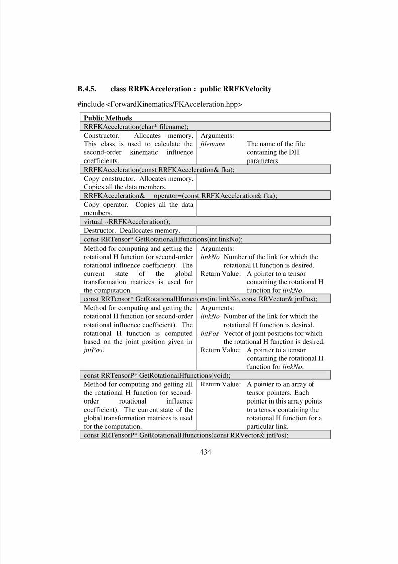
8/3/2019 Chetan Kapoor Dissertation
http://slidepdf.com/reader/full/chetan-kapoor-dissertation 455/612
434
B.4.5. class RRFKAcceleration : public RRFKVelocity
#include <ForwardKinematics/FKAcceleration.hpp>
Public Methods
RRFKAcceleration(char* filename);
Constructor. Allocates memory.This class is used to calculate thesecond-order kinematic influencecoefficients.
Arguments:
filename The name of the filecontaining the DHparameters.
RRFKAcceleration(const RRFKAcceleration& fka);
Copy constructor. Allocates memory.Copies all the data members.
RRFKAcceleration& operator=(const RRFKAcceleration& fka);Copy operator. Copies all the datamembers.
virtual ~RRFKAcceleration();
Destructor. Deallocates memory.
const RRTensor* GetRotationalHfunctions(int linkNo);
Method for computing and getting therotational H function (or second-orderrotational influence coefficient). Thecurrent state of the globaltransformation matrices is used forthe computation.
Arguments:
linkNo Number of the link for which therotational H function is desired.
Return Value: A pointer to a tensorcontaining the rotational Hfunction for linkNo.
const RRTensor* GetRotationalHfunctions(int linkNo, const RRVector& jntPos);
Method for computing and getting therotational H function (or second-orderrotational influence coefficient). Therotational H function is computedbased on the joint position given in
jntPos.
Arguments:
linkNo Number of the link for which therotational H function is desired.
jntPos Vector of joint positions for whichthe rotational H function is desired.
Return Value: A pointer to a tensorcontaining the rotational Hfunction for linkNo.
const RRTensorP* GetRotationalHfunctions(void);
Method for computing and getting all
the rotational H function (or second-order rotational influencecoefficient). The current state of theglobal transformation matrices is usedfor the computation.
Return Value: A pointer to an array of
tensor pointers. Eachpointer in this array pointsto a tensor containing therotational H function for aparticular link.
const RRTensorP* GetRotationalHfunctions(const RRVector& jntPos);
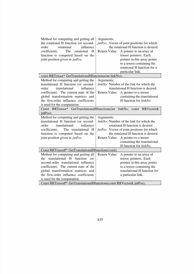
8/3/2019 Chetan Kapoor Dissertation
http://slidepdf.com/reader/full/chetan-kapoor-dissertation 456/612
435
Method for computing and getting allthe rotational H function (or second-
order rotational influencecoefficient). The rotational Hfunction is computed based on the joint position given in jntPos.
Arguments:
jntPos Vector of joint positions for which
the rotational H function is desired.Return Value: A pointer to an array of
tensor pointers. Eachpointer in this array pointsto a tensor containing therotational H function for aparticular link.
const RRTensor* GetTranslationalHfunctions(int linkNo);
Method for computing and getting thetranslational H function (or second-order translational influencecoefficient). The current state of the
global transformation matrices andthe first-order influence coefficientsis used for the computation.
Arguments:
linkNo Number of the link for which thetranslational H function is desired.
Return Value: A pointer to a tensor
containing the translationalH function for linkNo.
Const RRTensor* GetTranslationalHfunctions(int linkNo, const RRVector& jntPos);
Method for computing and getting thetranslational H function (or second-order translational influencecoefficient). The translational Hfunction is computed based on the joint position given in jntPos.
Arguments:
linkNo Number of the link for which therotational H function is desired.
jntPos Vector of joint positions for whichthe rotational H function is desired.
Return Value: A pointer to a tensorcontaining the translationalH function for linkNo.
Const RRTensorP* GetTranslationalHfunctions(void);
Method for computing and getting allthe translational H function (orsecond-order translational influencecoefficient). The current state of theglobal transformation matrices andthe first-order influence coefficientsis used for the computation.
Return Value: A pointer to an array of tensor pointers. Eachpointer in this array pointsto a tensor containing thetranslational H function fora particular link.
Const RRTensorP* GetTranslationalHfunctions(const RRVector& jntPos);

8/3/2019 Chetan Kapoor Dissertation
http://slidepdf.com/reader/full/chetan-kapoor-dissertation 457/612
436
Method for computing and getting allthe translational H function (or
second-order translational influencecoefficient). The translational Hfunction is computed based on the joint position given in jntPos.
Arguments:
jntPos Vector of joint positions for which
the translational H function isdesired.
Return Value: A pointer to an array of tensor pointers. Eachpointer in this array pointsto a tensor containing thetranslational H function fora particular link.
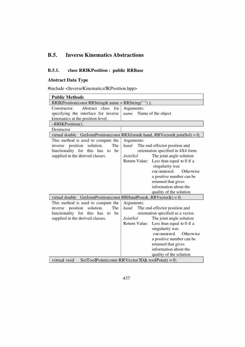
8/3/2019 Chetan Kapoor Dissertation
http://slidepdf.com/reader/full/chetan-kapoor-dissertation 458/612
437
B.5. Inverse Kinematics Abstractions
B.5.1. class RRIKPosition : public RRBase
Abstract Data Type
#include <InverseKinematics/IKPosition.hpp>
Public Methods
RRIKPosition(const RRString& name = RRString(" ") );
Constructor. Abstract class forspecifying the interface for inversekinematics at the position-level.
Arguments:name Name of the object
~RRIKPosition();
Destructor
virtual double GetJointPosition(const RRXform& hand, RRVector& jointSol) = 0;
This method is used to compute theinverse position solution. Thefunctionality for this has to besupplied in the derived classes.
Arguments:
hand The end-effector position andorientation specified in 4X4 form.
JointSol The joint angle solutionReturn Value: Less than equal to 0 if a
singularity wasencountered. Otherwisea positive number can be
returned that givesinformation about thequality of the solution
virtual double GetJointPosition(const RRHandPose&, RRVector&) = 0;
This method is used to compute theinverse position solution. Thefunctionality for this has to besupplied in the derived classes.
Arguments:hand The end-effector position and
orientation specified as a vector. JointSol The joint angle solutionReturn Value: Less than equal to 0 if a
singularity wasencountered. Otherwise
a positive number can be
returned that givesinformation about thequality of the solution
virtual void SetToolPoint(const RRVector3D& toolPoint) = 0;
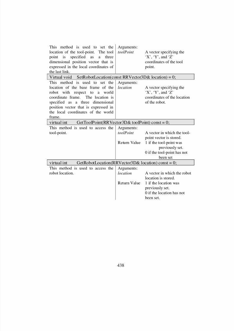
8/3/2019 Chetan Kapoor Dissertation
http://slidepdf.com/reader/full/chetan-kapoor-dissertation 459/612
438
This method is used to set thelocation of the tool-point. The tool
point is specified as a threedimensional position vector that isexpressed in the local coordinates of the last link.
Arguments:
toolPoint A vector specifying the
‘X’, ‘Y’, and ‘Z’coordinates of the toolpoint.
Virtual void SetRobotLocation(const RRVector3D& location) = 0;This method is used to set thelocation of the base frame of therobot with respect to a worldcoordinate frame. The location isspecified as a three dimensionalposition vector that is expressed inthe local coordinates of the world
frame.
Arguments:
location A vector specifying the‘X’, ‘Y’, and ‘Z’coordinates of the locationof the robot.
virtual int GetToolPoint(RRVector3D& toolPoint) const = 0;This method is used to access thetool-point.
Arguments:
toolPoint A vector in which the tool-point vector is stored.
Return Value 1 if the tool-point waspreviously set.
0 if the tool-point has notbeen set
virtual int GetRobotLocation(RRVector3D& location) const = 0;This method is used to access the
robot location.
Arguments:
location A vector in which the robotlocation is stored.
Return Value 1 if the location waspreviously set.0 if the location has notbeen set.
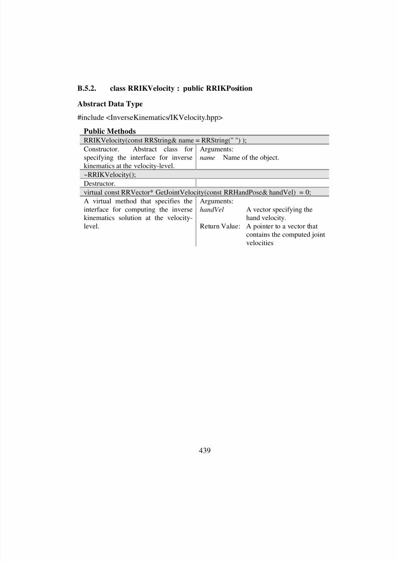
8/3/2019 Chetan Kapoor Dissertation
http://slidepdf.com/reader/full/chetan-kapoor-dissertation 460/612
439
B.5.2. class RRIKVelocity : public RRIKPosition
Abstract Data Type
#include <InverseKinematics/IKVelocity.hpp>
Public Methods
RRIKVelocity(const RRString& name = RRString(" ") );
Constructor. Abstract class forspecifying the interface for inversekinematics at the velocity-level.
Arguments:
name Name of the object.
~RRIKVelocity();
Destructor.
virtual const RRVector* GetJointVelocity(const RRHandPose& handVel) = 0;
A virtual method that specifies theinterface for computing the inversekinematics solution at the velocity-level.
Arguments:
handVel A vector specifying thehand velocity.
Return Value: A pointer to a vector thatcontains the computed jointvelocities
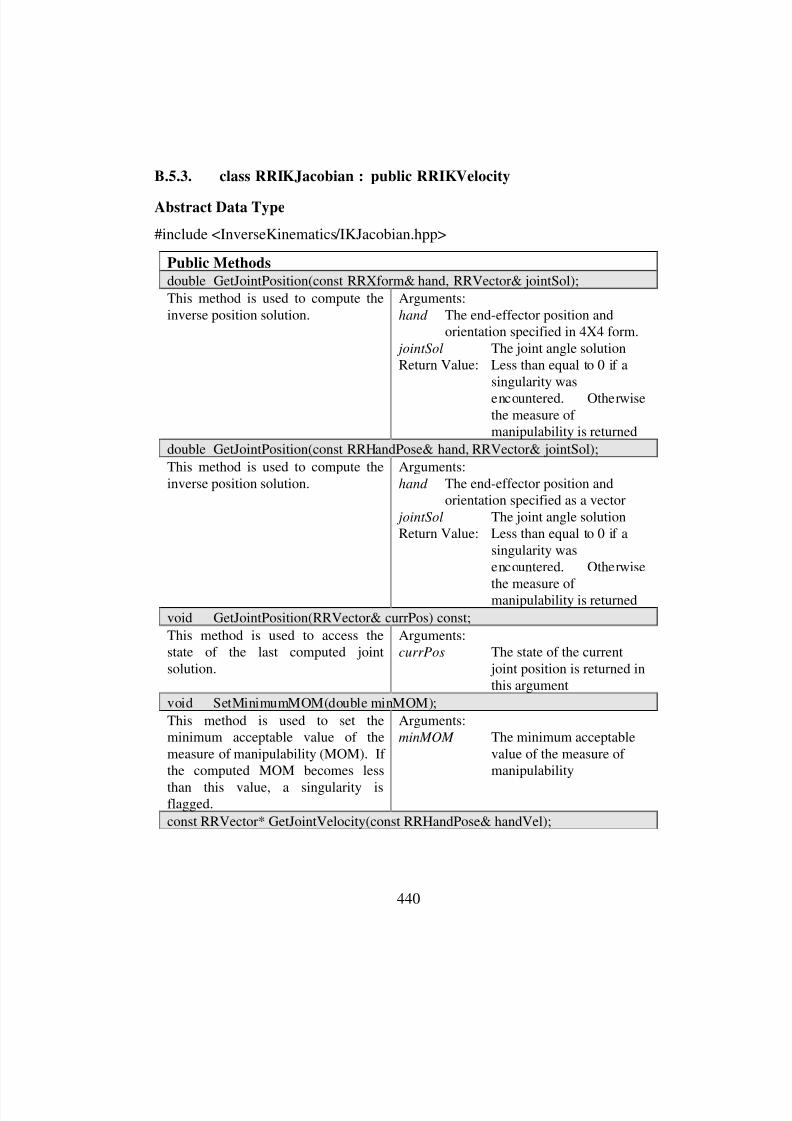
8/3/2019 Chetan Kapoor Dissertation
http://slidepdf.com/reader/full/chetan-kapoor-dissertation 461/612
440
B.5.3. class RRIKJacobian : public RRIKVelocity
Abstract Data Type
#include <InverseKinematics/IKJacobian.hpp>
Public Methods
double GetJointPosition(const RRXform& hand, RRVector& jointSol);
This method is used to compute theinverse position solution.
Arguments:
hand The end-effector position andorientation specified in 4X4 form.
jointSol The joint angle solutionReturn Value: Less than equal to 0 if a
singularity was
encountered. Otherwisethe measure of manipulability is returned
double GetJointPosition(const RRHandPose& hand, RRVector& jointSol);
This method is used to compute theinverse position solution.
Arguments:
hand The end-effector position andorientation specified as a vector
jointSol The joint angle solutionReturn Value: Less than equal to 0 if a
singularity wasencountered. Otherwise
the measure of manipulability is returned
void GetJointPosition(RRVector& currPos) const;
This method is used to access thestate of the last computed jointsolution.
Arguments:currPos The state of the current
joint position is returned inthis argument
void SetMinimumMOM(double minMOM);
This method is used to set theminimum acceptable value of themeasure of manipulability (MOM). If the computed MOM becomes less
than this value, a singularity isflagged.
Arguments:minMOM The minimum acceptable
value of the measure of manipulability
const RRVector* GetJointVelocity(const RRHandPose& handVel);

8/3/2019 Chetan Kapoor Dissertation
http://slidepdf.com/reader/full/chetan-kapoor-dissertation 462/612
441
A method for computing the jointvelocities corresponding to a desired
hand velocity. This method should becalled after a successful call toGetJointPosition.
Arguments:
handVel A vector specifying the
hand velocity.Return Value: A pointer to a vector that
contains the computed jointvelocities
void SetToolPoint(const RRVector3D& toolPoint);
This method is used to set thelocation of the tool-point. The toolpoint is specified as a threedimensional position vector that isexpressed in the local coordinates of the last link.
Arguments:toolPoint A vector specifying the
‘X’, ‘Y’, and ‘Z’coordinates of the toolpoint.
void SetRobotLocation(const RRVector3D& location);
This method is used to set thelocation of the base frame of therobot with respect to a worldcoordinate frame. The location isspecified as a three dimensionalposition vector that is expressed inthe local coordinates of the worldframe.
Arguments:location A vector specifying the
‘X’, ‘Y’, and ‘Z’coordinates of the locationof the robot.
int SetJointPosition(const RRVector& jointPos);
This method is used to set the currentstate of the joint positions of therobot. This method is similar toresetting the initial jointconfiguration.
Arguments: jointPos A vector specifying the
current joint position of therobot.
int GetToolPoint(RRVector3D& toolPoint) const;
This method is used to access thetool-point.
Arguments:toolPoint A vector in which the tool-
point vector is stored.Return Value 1 if the tool-point was
previously set.0 if the tool-point has notbeen set
int GetRobotLocation(RRVector3D& location) const;
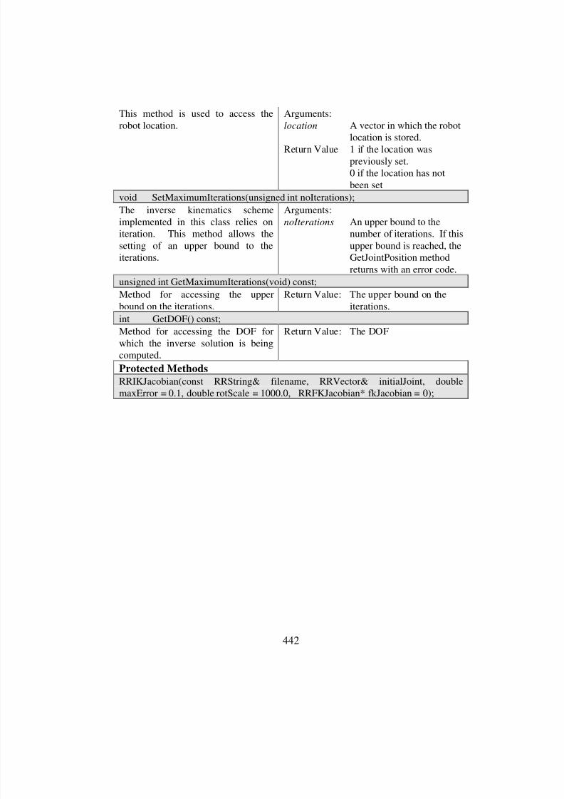
8/3/2019 Chetan Kapoor Dissertation
http://slidepdf.com/reader/full/chetan-kapoor-dissertation 463/612
442
This method is used to access therobot location.
Arguments:
location A vector in which the robot
location is stored.Return Value 1 if the location was
previously set.0 if the location has notbeen set
void SetMaximumIterations(unsigned int noIterations);
The inverse kinematics schemeimplemented in this class relies oniteration. This method allows thesetting of an upper bound to theiterations.
Arguments:
noIterations An upper bound to thenumber of iterations. If thisupper bound is reached, theGetJointPosition methodreturns with an error code.
unsigned int GetMaximumIterations(void) const;Method for accessing the upperbound on the iterations.
Return Value: The upper bound on theiterations.
int GetDOF() const;
Method for accessing the DOF forwhich the inverse solution is beingcomputed.
Return Value: The DOF
Protected Methods
RRIKJacobian(const RRString& filename, RRVector& initialJoint, doublemaxError = 0.1, double rotScale = 1000.0, RRFKJacobian* fkJacobian = 0);
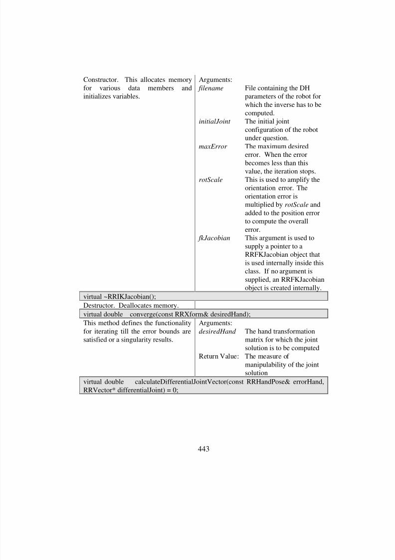
8/3/2019 Chetan Kapoor Dissertation
http://slidepdf.com/reader/full/chetan-kapoor-dissertation 464/612
443
Constructor. This allocates memoryfor various data members and
initializes variables.
Arguments:
filename File containing the DH
parameters of the robot forwhich the inverse has to becomputed.
initialJoint The initial jointconfiguration of the robotunder question.
maxError The maximum desirederror. When the errorbecomes less than thisvalue, the iteration stops.
rotScale This is used to amplify theorientation error. The
orientation error ismultiplied by rotScale andadded to the position errorto compute the overallerror.
fkJacobian This argument is used tosupply a pointer to aRRFKJacobian object thatis used internally inside thisclass. If no argument issupplied, an RRFKJacobianobject is created internally.
virtual ~RRIKJacobian();Destructor. Deallocates memory.
virtual double converge(const RRXform& desiredHand);
This method defines the functionalityfor iterating till the error bounds aresatisfied or a singularity results.
Arguments:
desiredHand The hand transformationmatrix for which the jointsolution is to be computed
Return Value: The measure of manipulability of the jointsolution
virtual double calculateDifferentialJointVector(const RRHandPose& errorHand,
RRVector* differentialJoint) = 0;
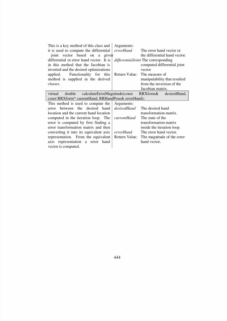
8/3/2019 Chetan Kapoor Dissertation
http://slidepdf.com/reader/full/chetan-kapoor-dissertation 465/612
444
This is a key method of this class andit is used to compute the differential
joint vector based on a givendifferential or error hand vector. It isin this method that the Jacobian isinverted and the desired optimizationsapplied. Functionality for thismethod is supplied in the derivedclasses.
Arguments:
errorHand The error hand vector or
the differential hand vector.differentialJoint The corresponding
computed differential jointvector
Return Value: The measure of manipulability that resultedfrom the inversion of theJacobian matrix.
virtual double calculateErrorMagnitude(const RRXform& desiredHand,const RRXform* currentHand, RRHandPose& errorHand);
This method is used to compute theerror between the desired hand
location and the current hand locationcomputed in the iteration loop. Theerror is computed by first finding aerror transformation matrix and thenconverting it into its equivalent axisrepresentation. From the equivalentaxis representation a error handvector is computed.
Arguments:
desiredHand The desired hand
transformation matrix.currentHand The state of the
transformation matrixinside the iteration loop.
errorHand The error hand vector.Return Value: The magnitude of the error
hand vector.
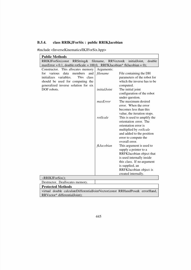
8/3/2019 Chetan Kapoor Dissertation
http://slidepdf.com/reader/full/chetan-kapoor-dissertation 466/612
445
B.5.4. class RRIKJForSix : public RRIKJacobian
#include <InverseKinematics/IKJForSix.hpp>
Public Methods
RRIKJForSix(const RRString& filename, RRVector& initialJoint, doublemaxError = 0.1, double rotScale = 100.0, RRFKJacobian* fkJacobian = 0);
Constructor. This allocates memoryfor various data members andinitializes variables. This classshould be used for computing thegeneralized inverse solution for sixDOF robots.
Arguments:
filename File containing the DHparameters of the robot forwhich the inverse has to becomputed.
initialJoint The initial joint
configuration of the robotunder question.maxError The maximum desired
error. When the errorbecomes less than thisvalue, the iteration stops.
rotScale This is used to amplify theorientation error. Theorientation error ismultiplied by rotScale
and added to the positionerror to compute the
overall error. fkJacobian This argument is used to
supply a pointer to aRRFKJacobian object thatis used internally insidethis class. If no argumentis supplied, anRRFKJacobian object iscreated internally.
~RRIKJForSix();
Destructor. Deallocates memory.
Protected Methods
virtual double calculateDifferentialJointVector(const RRHandPose& errorHand,RRVector* differentialJoint);

8/3/2019 Chetan Kapoor Dissertation
http://slidepdf.com/reader/full/chetan-kapoor-dissertation 467/612
446
This method computes thedifferential joint vector by
multiplying the error hand vectorwith the inverse of the Jacobianmatrix.
Arguments:
errorHand The error hand vector or
the differential handvector.
differentialJoint The correspondingcomputed differential jointvector
Return Value: The measure of manipulability that resultedfrom the inversion of theJacobian matrix.

8/3/2019 Chetan Kapoor Dissertation
http://slidepdf.com/reader/full/chetan-kapoor-dissertation 468/612
447
B.5.5. class RRIKJForGTSix : public RRIKJacobian
#include <InverseKinematics/IKJForGTSix.hpp>
Public Methods
RRIKJForGTSix(const RRString& filename, RRVector& initialJoint, doublemaxError = 0.1, double rotScale = 100.0, RRFKJacobian* fkJacobian = 0);
Constructor. This allocates memoryfor various data members andinitializes variables. This classshould be used for computing thegeneralized inverse solution for serialrobots with greater than six DOF
robots.
Arguments:
filename File containing the DHparameters of the robot forwhich the inverse has to becomputed.
initialJoint The initial joint
configuration of the robotunder question.maxError The maximum desired
error. When the errorbecomes less than thisvalue, the iteration stops.
rotScale This is used to amplify theorientation error. Theorientation error ismultiplied by rotScale
and added to the positionerror to compute the
overall error. fkJacobian This argument is used to
supply a pointer to aRRFKJacobian object thatis used internally insidethis class. If no argumentis supplied, anRRFKJacobian object iscreated internally.
~RRIKJForGTSix();
Destructor. Deallocates memory.
Protected Methods
virtual double calculateDifferentialJointVector(const RRHandPose& errorHand,RRVector* differentialJoint);
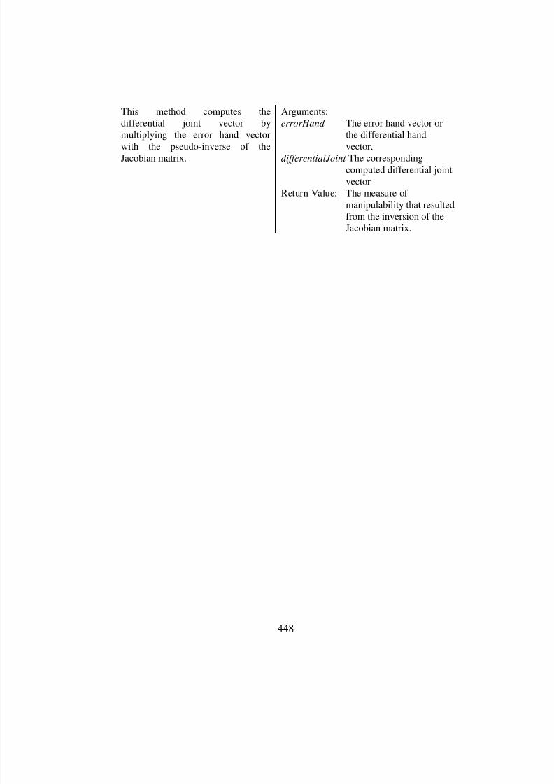
8/3/2019 Chetan Kapoor Dissertation
http://slidepdf.com/reader/full/chetan-kapoor-dissertation 469/612
448
This method computes thedifferential joint vector by
multiplying the error hand vectorwith the pseudo-inverse of theJacobian matrix.
Arguments:
errorHand The error hand vector or
the differential handvector.
differentialJoint The correspondingcomputed differential jointvector
Return Value: The measure of manipulability that resultedfrom the inversion of theJacobian matrix.
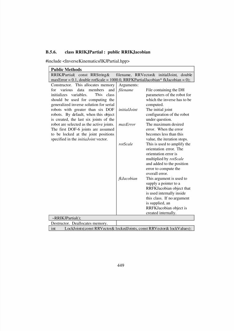
8/3/2019 Chetan Kapoor Dissertation
http://slidepdf.com/reader/full/chetan-kapoor-dissertation 470/612
449
B.5.6. class RRIKJPartial : public RRIKJacobian
#include <InverseKinematics/IKJPartial.hpp>
Public Methods
RRIKJPartial( const RRString& filename, RRVector& initialJoint, doublemaxError = 0.1, double rotScale = 1000.0, RRFKPartialJacobian* fkJacobian = 0);
Constructor. This allocates memoryfor various data members andinitializes variables. This classshould be used for computing thegeneralized inverse solution for serialrobots with greater than six DOF
robots. By default, when this objectis created, the last six joints of therobot are selected as the active joints.The first DOF-6 joints are assumedto be locked at the joint positionsspecified in the initiaJoint vector.
Arguments:
filename File containing the DHparameters of the robot forwhich the inverse has to becomputed.
initialJoint The initial joint
configuration of the robotunder question.maxError The maximum desired
error. When the errorbecomes less than thisvalue, the iteration stops.
rotScale This is used to amplify theorientation error. Theorientation error ismultiplied by rotScale
and added to the positionerror to compute the
overall error. fkJacobian This argument is used to
supply a pointer to aRRFKJacobian object thatis used internally insidethis class. If no argumentis supplied, anRRFKJacobian object iscreated internally.
~RRIKJPartial();
Destructor. Deallocates memory.
int LockJoints(const RRVector& lockedJoints, const RRVector& lockValues);
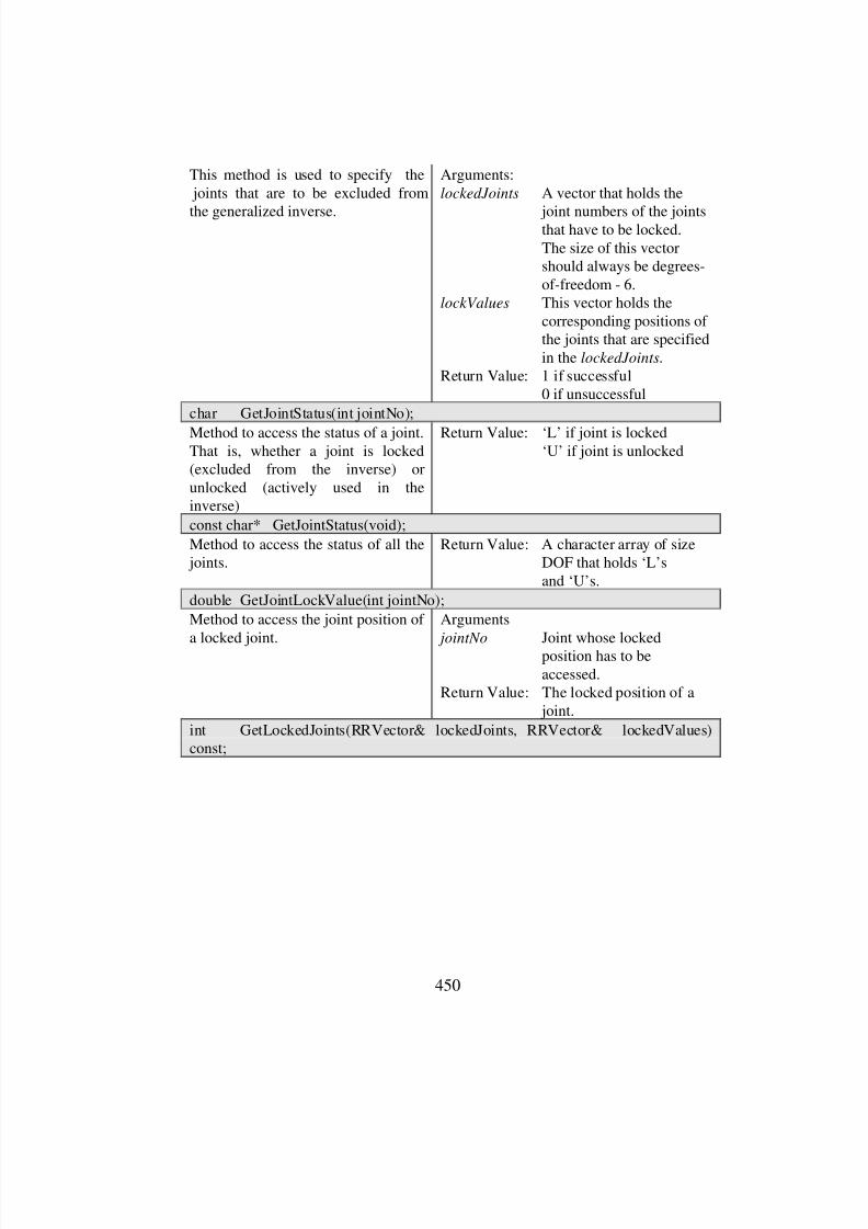
8/3/2019 Chetan Kapoor Dissertation
http://slidepdf.com/reader/full/chetan-kapoor-dissertation 471/612
450
This method is used to specify the joints that are to be excluded from
the generalized inverse.
Arguments:
lockedJoints A vector that holds the
joint numbers of the jointsthat have to be locked.The size of this vectorshould always be degrees-of-freedom - 6.
lockValues This vector holds thecorresponding positions of the joints that are specifiedin the lockedJoints.
Return Value: 1 if successful0 if unsuccessful
char GetJointStatus(int jointNo);
Method to access the status of a joint.That is, whether a joint is locked(excluded from the inverse) orunlocked (actively used in theinverse)
Return Value: ‘L’ if joint is locked‘U’ if joint is unlocked
const char* GetJointStatus(void);
Method to access the status of all the joints.
Return Value: A character array of sizeDOF that holds ‘L’sand ‘U’s.
double GetJointLockValue(int jointNo);
Method to access the joint position of a locked joint.
Arguments
jointNo Joint whose lockedposition has to beaccessed.
Return Value: The locked position of a joint.
int GetLockedJoints(RRVector& lockedJoints, RRVector& lockedValues)const;
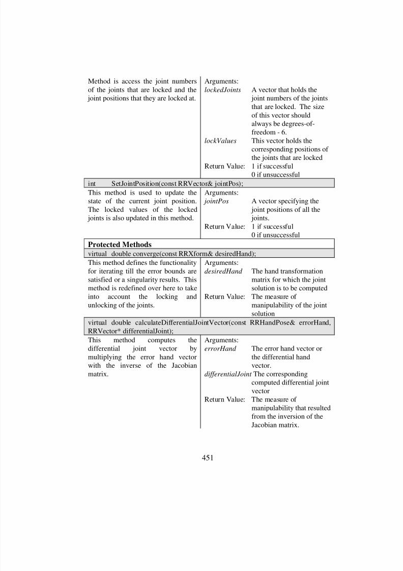
8/3/2019 Chetan Kapoor Dissertation
http://slidepdf.com/reader/full/chetan-kapoor-dissertation 472/612
451
Method is access the joint numbersof the joints that are locked and the
joint positions that they are locked at.
Arguments:
lockedJoints A vector that holds the
joint numbers of the jointsthat are locked. The sizeof this vector shouldalways be degrees-of-freedom - 6.
lockValues This vector holds thecorresponding positions of the joints that are locked
Return Value: 1 if successful0 if unsuccessful
int SetJointPosition(const RRVector& jointPos);
This method is used to update the
state of the current joint position.The locked values of the locked joints is also updated in this method.
Arguments:
jointPos A vector specifying the joint positions of all the joints.
Return Value: 1 if successful0 if unsuccessful
Protected Methods
virtual double converge(const RRXform& desiredHand);
This method defines the functionalityfor iterating till the error bounds aresatisfied or a singularity results. Thismethod is redefined over here to take
into account the locking andunlocking of the joints.
Arguments:
desiredHand The hand transformationmatrix for which the jointsolution is to be computed
Return Value: The measure of manipulability of the jointsolution
virtual double calculateDifferentialJointVector(const RRHandPose& errorHand,RRVector* differentialJoint);
This method computes thedifferential joint vector bymultiplying the error hand vectorwith the inverse of the Jacobianmatrix.
Arguments:errorHand The error hand vector or
the differential handvector.
differentialJoint The correspondingcomputed differential jointvector
Return Value: The measure of manipulability that resultedfrom the inversion of theJacobian matrix.
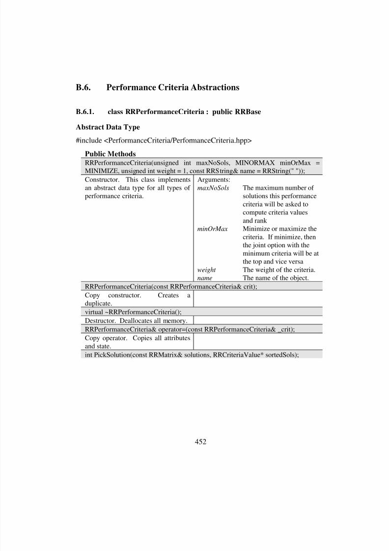
8/3/2019 Chetan Kapoor Dissertation
http://slidepdf.com/reader/full/chetan-kapoor-dissertation 473/612
452
B.6. Performance Criteria Abstractions
B.6.1. class RRPerformanceCriteria : public RRBase
Abstract Data Type
#include <PerformanceCriteria/PerformanceCriteria.hpp>
Public Methods
RRPerformanceCriteria(unsigned int maxNoSols, MINORMAX minOrMax =MINIMIZE, unsigned int weight = 1, const RRString& name = RRString(" "));
Constructor. This class implementsan abstract data type for all types of performance criteria.
Arguments:
maxNoSols The maximum number of solutions this performancecriteria will be asked tocompute criteria valuesand rank
minOrMax Minimize or maximize thecriteria. If minimize, thenthe joint option with theminimum criteria will be atthe top and vice versa
weight The weight of the criteria.name The name of the object.
RRPerformanceCriteria(const RRPerformanceCriteria& crit);Copy constructor. Creates aduplicate.
virtual ~RRPerformanceCriteria();
Destructor. Deallocates all memory.
RRPerformanceCriteria& operator=(const RRPerformanceCriteria& _crit);
Copy operator. Copies all attributesand state.
int PickSolution(const RRMatrix& solutions, RRCriteriaValue* sortedSols);
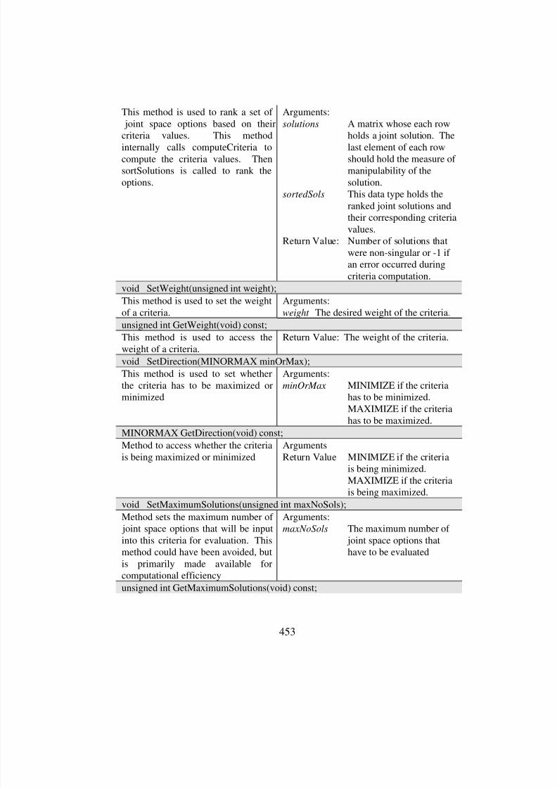
8/3/2019 Chetan Kapoor Dissertation
http://slidepdf.com/reader/full/chetan-kapoor-dissertation 474/612
453
This method is used to rank a set of joint space options based on their
criteria values. This methodinternally calls computeCriteria tocompute the criteria values. ThensortSolutions is called to rank theoptions.
Arguments:
solutions A matrix whose each row
holds a joint solution. Thelast element of each rowshould hold the measure of manipulability of thesolution.
sortedSols This data type holds theranked joint solutions andtheir corresponding criteriavalues.
Return Value: Number of solutions thatwere non-singular or -1 if an error occurred during
criteria computation.void SetWeight(unsigned int weight);
This method is used to set the weightof a criteria.
Arguments:
weight The desired weight of the criteria.
unsigned int GetWeight(void) const;
This method is used to access theweight of a criteria.
Return Value: The weight of the criteria.
void SetDirection(MINORMAX minOrMax);
This method is used to set whetherthe criteria has to be maximized orminimized
Arguments:
minOrMax MINIMIZE if the criteriahas to be minimized.MAXIMIZE if the criteriahas to be maximized.
MINORMAX GetDirection(void) const;
Method to access whether the criteriais being maximized or minimized
ArgumentsReturn Value MINIMIZE if the criteria
is being minimized.MAXIMIZE if the criteriais being maximized.
void SetMaximumSolutions(unsigned int maxNoSols);
Method sets the maximum number of joint space options that will be inputinto this criteria for evaluation. This
method could have been avoided, butis primarily made available forcomputational efficiency
Arguments:maxNoSols The maximum number of
joint space options that
have to be evaluated
unsigned int GetMaximumSolutions(void) const;

8/3/2019 Chetan Kapoor Dissertation
http://slidepdf.com/reader/full/chetan-kapoor-dissertation 475/612
454
Method accesses the maximumnumber of joint space options that
will be input into this criteria forevaluation. This method could havebeen avoided, but is primarily madeavailable for computationalefficiency
Arguments:
maxNoSols The maximum number of
joint space options thathave to be evaluated
Protected Methods
virtual unsigned int sortSolutions(RRCriteriaValue* critVals, unsigned int noSols);
This method sorts the various criteriavalues and the joint space optionsassociated with them. It utilizes aquick sort to do the sorting. Derivedclasses can redefine the sorting
functionality.
Arguments:critVals A dual vector of criteria
values and the joint spaceoptions that has to besorted.
noSols No of solutions to besorted.
Return Value: The number of the bestsolution.
virtual int computeCriteria(const RRMatrix& sols, RRCriteriaValue* critVals) = 0;
This pure virtual method provides theinterface for computing the criteriavalues based on a given set of solutions. Functionality to computethe criteria value is to be provided inderived classes.
Arguments:
sols The solutions to be sorted. Eachrow of this matrix holds a solutionwith the last element of each rowholding he measure of manipulability of the solution..
crtiVals The computed criteriavalues and the associatedsolution number go in this.This array should be of size equal to the number of rows of sols.
Return Value: 0 if all solutions aresingular-1 if an error occurred incriteria computation.1 if okay.
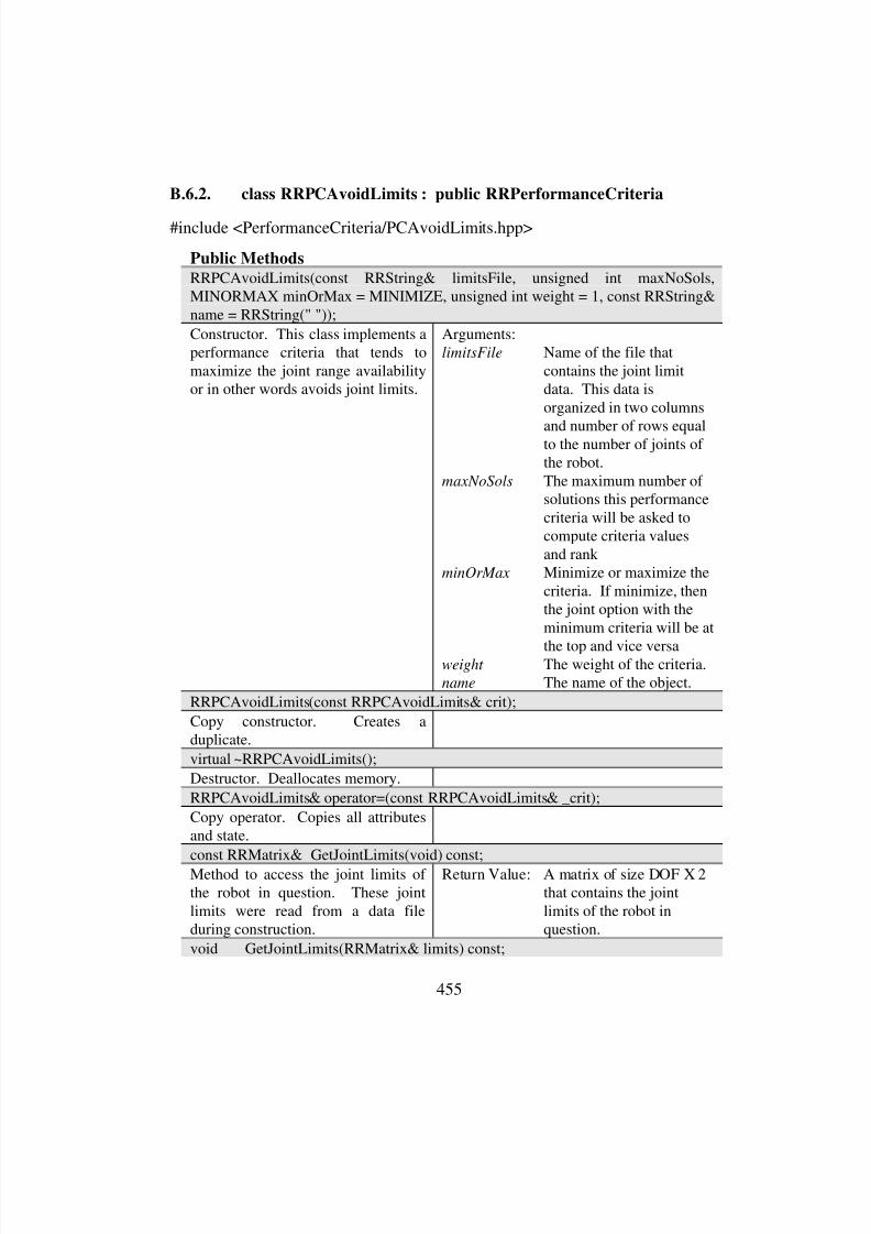
8/3/2019 Chetan Kapoor Dissertation
http://slidepdf.com/reader/full/chetan-kapoor-dissertation 476/612
455
B.6.2. class RRPCAvoidLimits : public RRPerformanceCriteria
#include <PerformanceCriteria/PCAvoidLimits.hpp>
Public Methods
RRPCAvoidLimits(const RRString& limitsFile, unsigned int maxNoSols,MINORMAX minOrMax = MINIMIZE, unsigned int weight = 1, const RRString&name = RRString(" "));
Constructor. This class implements aperformance criteria that tends tomaximize the joint range availabilityor in other words avoids joint limits.
Arguments:limitsFile Name of the file that
contains the joint limitdata. This data isorganized in two columns
and number of rows equalto the number of joints of the robot.
maxNoSols The maximum number of solutions this performancecriteria will be asked tocompute criteria valuesand rank
minOrMax Minimize or maximize thecriteria. If minimize, thenthe joint option with theminimum criteria will be at
the top and vice versaweight The weight of the criteria.name The name of the object.
RRPCAvoidLimits(const RRPCAvoidLimits& crit);
Copy constructor. Creates aduplicate.
virtual ~RRPCAvoidLimits();
Destructor. Deallocates memory.
RRPCAvoidLimits& operator=(const RRPCAvoidLimits& _crit);
Copy operator. Copies all attributesand state.
const RRMatrix& GetJointLimits(void) const;
Method to access the joint limits of the robot in question. These jointlimits were read from a data fileduring construction.
Return Value: A matrix of size DOF X 2that contains the jointlimits of the robot inquestion.
void GetJointLimits(RRMatrix& limits) const;
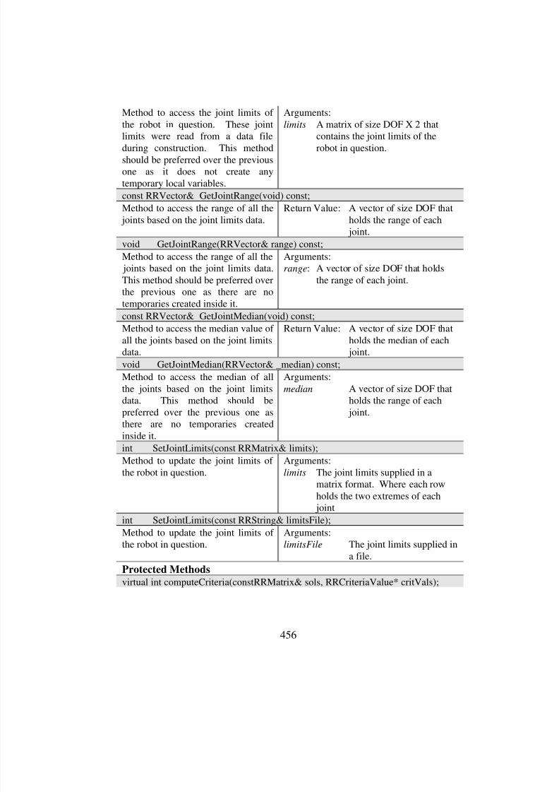
8/3/2019 Chetan Kapoor Dissertation
http://slidepdf.com/reader/full/chetan-kapoor-dissertation 477/612
456
Method to access the joint limits of the robot in question. These joint
limits were read from a data fileduring construction. This methodshould be preferred over the previousone as it does not create anytemporary local variables.
Arguments:
limits A matrix of size DOF X 2 that
contains the joint limits of therobot in question.
const RRVector& GetJointRange(void) const;
Method to access the range of all the joints based on the joint limits data.
Return Value: A vector of size DOF thatholds the range of each joint.
void GetJointRange(RRVector& range) const;
Method to access the range of all the joints based on the joint limits data.
This method should be preferred overthe previous one as there are notemporaries created inside it.
Arguments:range: A vector of size DOF that holds
the range of each joint.
const RRVector& GetJointMedian(void) const;
Method to access the median value of all the joints based on the joint limitsdata.
Return Value: A vector of size DOF thatholds the median of each joint.
void GetJointMedian(RRVector& _median) const;
Method to access the median of allthe joints based on the joint limitsdata. This method should be
preferred over the previous one asthere are no temporaries createdinside it.
Arguments:
median A vector of size DOF thatholds the range of each
joint.
int SetJointLimits(const RRMatrix& limits);
Method to update the joint limits of the robot in question.
Arguments:
limits The joint limits supplied in amatrix format. Where each rowholds the two extremes of each joint
int SetJointLimits(const RRString& limitsFile);
Method to update the joint limits of the robot in question.
Arguments:limitsFile The joint limits supplied in
a file.Protected Methods
virtual int computeCriteria(constRRMatrix& sols, RRCriteriaValue* critVals);
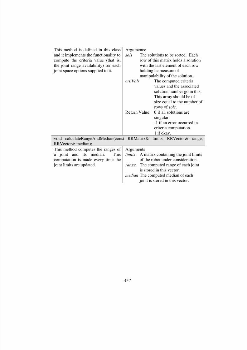
8/3/2019 Chetan Kapoor Dissertation
http://slidepdf.com/reader/full/chetan-kapoor-dissertation 478/612
457
This method is defined in this classand it implements the functionality to
compute the criteria value (that is,the joint range availability) for each joint space options supplied to it.
Arguments:
sols The solutions to be sorted. Each
row of this matrix holds a solutionwith the last element of each rowholding he measure of manipulability of the solution..
crtiVals The computed criteriavalues and the associatedsolution number go in this.This array should be of size equal to the number of rows of sols.
Return Value: 0 if all solutions aresingular
-1 if an error occurred incriteria computation.1 if okay.
void calculateRangeAndMedian(const RRMatrix& limits, RRVector& range,RRVector& median);
This method computes the ranges of a joint and its median. Thiscomputation is made every time the joint limits are updated.
Argumentslimits A matrix containing the joint limits
of the robot under consideration.range The computed range of each joint
is stored in this vector.median The computed median of each
joint is stored in this vector.

8/3/2019 Chetan Kapoor Dissertation
http://slidepdf.com/reader/full/chetan-kapoor-dissertation 479/612
458
B.6.3. class RRPCMinimizeVelocity : public RRPerformanceCriteria
#include <PerformanceCriteria/PCMinimizeVelocity.hpp>
Public Methods
RRPCMinimizeVelocity(const RRVector& currPos, unsigned int maxNoSols,MINORMAX minOrMax = MINIMIZE, unsigned int weight = 1, const RRString&name = RRString(" "));
Constructor. This class implements aperformance criteria that tends tominimize the joint velocity. Thus,this criteria selects joint options thattend to minimize joint velocities.
Arguments:currPosThis specifies the current
joint position of the robot.The joint velocity for each joint space option is
computed by subtractingfrom currPos.maxNoSols The maximum number of
solutions this performancecriteria will be asked tocompute criteria valuesand rank
minOrMax Minimize or maximize thecriteria. If minimize, thenthe joint option with theminimum criteria will be atthe top and vice versa
weight The weight of the criteria.name The name of the object.
RRPCMinimizeVelocity(const RRPCMinimizeVelocity& crit);
Copy constructor. Creates aduplicate.
virtual ~RRPCMinimizeVelocity();
Destructor. Deallocates memory.
RRPCMinimizeVelocity& operator=(const RRPCMinimizeVelocity& _crit);
Copy operator. Copies all attributesand state.
int SetCurrentPosition(const RRVector& currPos);

8/3/2019 Chetan Kapoor Dissertation
http://slidepdf.com/reader/full/chetan-kapoor-dissertation 480/612
459
This method sets the state of thecurrent joint position of the robot.
This method should be called everytime before a call to the PickSolutionsmethod. The joint velocity criteriaare computed by comparing to thecurrent joint position of the robot setusing this method.
Arguments:
currPos A vector of size DOF that
specifies the current jointlocation of the robot.
Return Value: 1 if successful0 if unsuccessful
int GetCurrentPosition(RRVector& currPos) const;
This method is used to access thestate of the current joint position of the robot.
Arguments:currPos A vector of size DOF that
returns the current jointlocation of the robot.
Return Value: 1 if successful
0 if unsuccessfulProtected Methods
virtual int computeCriteria(const RRMatrix& sols, RRCriteriaValue* critVals);
This method is defined in this classand it implements the functionality tocompute the criteria value (that is, the joint velocity) for each joint spaceoptions supplied to it. It uses thecurrent joint position to compute the joint velocity for each option.
Arguments:
sols The solutions to be sorted. Eachrow of this matrix holds a solutionwith the last element of each rowholding he measure of manipulability of the solution..
crtiVals The computed criteriavalues and the associated
solution number go in this.This array should be of size equal to the number of rows of sols.
Return Value: 0 if all solutions aresingular-1 if an error occurred incriteria computation.1 if okay.
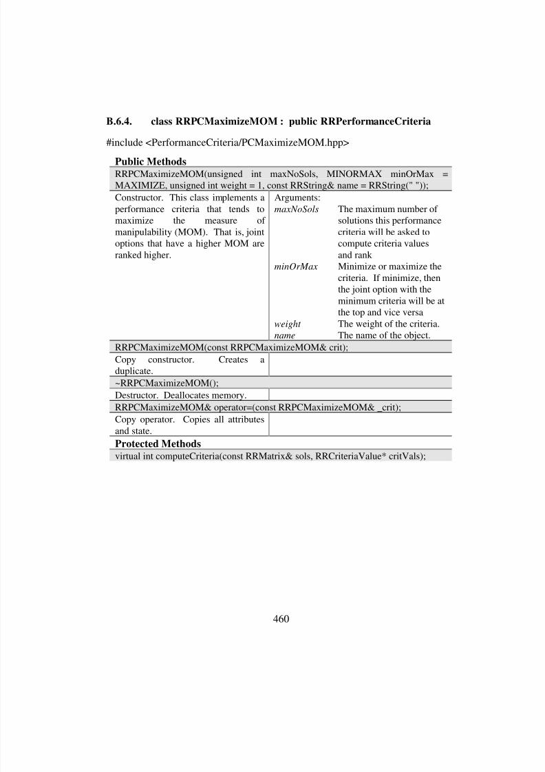
8/3/2019 Chetan Kapoor Dissertation
http://slidepdf.com/reader/full/chetan-kapoor-dissertation 481/612
460
B.6.4. class RRPCMaximizeMOM : public RRPerformanceCriteria
#include <PerformanceCriteria/PCMaximizeMOM.hpp>
Public Methods
RRPCMaximizeMOM(unsigned int maxNoSols, MINORMAX minOrMax =MAXIMIZE, unsigned int weight = 1, const RRString& name = RRString(" "));
Constructor. This class implements aperformance criteria that tends tomaximize the measure of manipulability (MOM). That is, jointoptions that have a higher MOM areranked higher.
Arguments:
maxNoSols The maximum number of solutions this performancecriteria will be asked tocompute criteria valuesand rank
minOrMax Minimize or maximize thecriteria. If minimize, thenthe joint option with theminimum criteria will be atthe top and vice versa
weight The weight of the criteria.name The name of the object.
RRPCMaximizeMOM(const RRPCMaximizeMOM& crit);
Copy constructor. Creates aduplicate.
~RRPCMaximizeMOM();
Destructor. Deallocates memory.
RRPCMaximizeMOM& operator=(const RRPCMaximizeMOM& _crit);Copy operator. Copies all attributesand state.
Protected Methods
virtual int computeCriteria(const RRMatrix& sols, RRCriteriaValue* critVals);
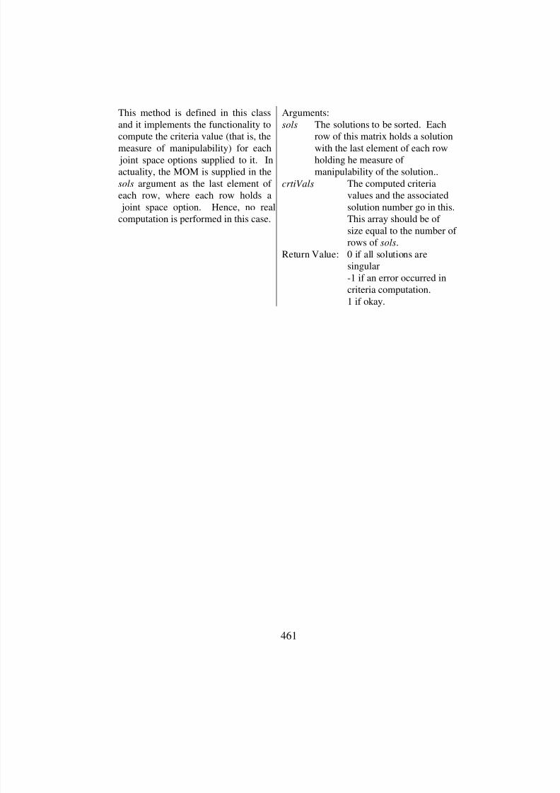
8/3/2019 Chetan Kapoor Dissertation
http://slidepdf.com/reader/full/chetan-kapoor-dissertation 482/612
461
This method is defined in this classand it implements the functionality to
compute the criteria value (that is, themeasure of manipulability) for each joint space options supplied to it. Inactuality, the MOM is supplied in the
sols argument as the last element of each row, where each row holds a joint space option. Hence, no realcomputation is performed in this case.
Arguments:
sols The solutions to be sorted. Each
row of this matrix holds a solutionwith the last element of each rowholding he measure of manipulability of the solution..
crtiVals The computed criteriavalues and the associatedsolution number go in this.This array should be of size equal to the number of rows of sols.
Return Value: 0 if all solutions aresingular
-1 if an error occurred incriteria computation.1 if okay.

8/3/2019 Chetan Kapoor Dissertation
http://slidepdf.com/reader/full/chetan-kapoor-dissertation 483/612
462
B.6.5. class RRPCFusion : public RRBase
#include <PerformanceCriteria/PCFusion.hpp>
Public Methods
RRPCFusion(RRPerformanceCriteria** critArray, unsigned int noCriteria, unsignedint maxNoSols, MINORMAX minOrMax = MAXIMIZE, const RRString& name =RRString(" "));
Constructor. This classimplements a data type for criteriafusion. A set of performancecriteria objects are supplied to thisclass. It uses a weighted sum
technique to first rank all jointspace options based on individualcriteria, and then it combines all of them to come up with an overallranking.
Arguments:critArray This holds a pointer to an
array of performancecriteria objects. Theseobjects constitute the
criteria that have to befused.noCriteria Number of criteria being
supplied in critArray.maxNoSols The maximum number of
solutions this performancecriteria will be asked tocompute criteria valuesand rank
minOrMax Minimize or maximize thecriteria. If minimize, thenthe joint option with the
minimum criteria will be atthe top and vice versa
weight The weight of the criteria.
name The name of the object.
virtual ~RRPCFusion();
Destructor. Deallocates memory.
int PickSolution(const RRMatrix& solutions, RRCriteriaValue* sortedSols);
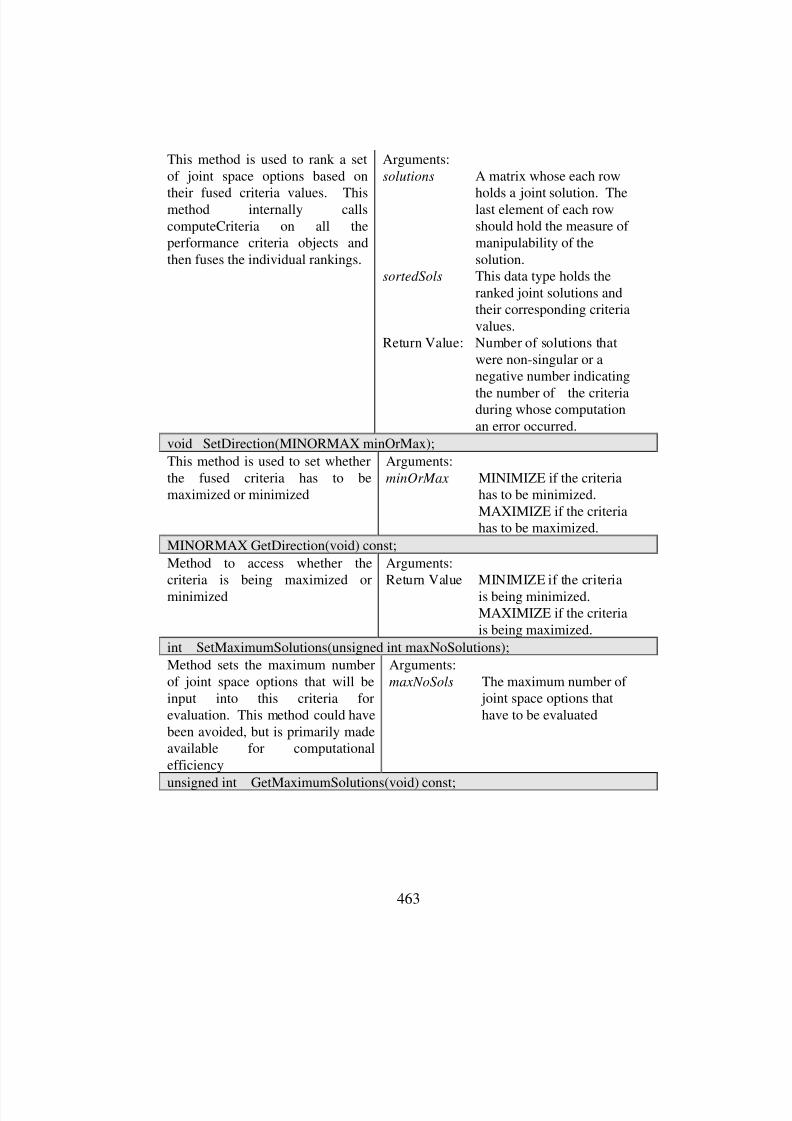
8/3/2019 Chetan Kapoor Dissertation
http://slidepdf.com/reader/full/chetan-kapoor-dissertation 484/612
463
This method is used to rank a setof joint space options based on
their fused criteria values. Thismethod internally callscomputeCriteria on all theperformance criteria objects andthen fuses the individual rankings.
Arguments:
solutions A matrix whose each row
holds a joint solution. Thelast element of each rowshould hold the measure of manipulability of thesolution.
sortedSols This data type holds theranked joint solutions andtheir corresponding criteriavalues.
Return Value: Number of solutions thatwere non-singular or anegative number indicating
the number of the criteriaduring whose computationan error occurred.
void SetDirection(MINORMAX minOrMax);
This method is used to set whetherthe fused criteria has to bemaximized or minimized
Arguments:
minOrMax MINIMIZE if the criteriahas to be minimized.MAXIMIZE if the criteriahas to be maximized.
MINORMAX GetDirection(void) const;
Method to access whether thecriteria is being maximized orminimized
Arguments:Return Value MINIMIZE if the criteria
is being minimized.MAXIMIZE if the criteriais being maximized.
int SetMaximumSolutions(unsigned int maxNoSolutions);
Method sets the maximum numberof joint space options that will beinput into this criteria forevaluation. This method could havebeen avoided, but is primarily madeavailable for computationalefficiency
Arguments:
maxNoSols The maximum number of joint space options thathave to be evaluated
unsigned int GetMaximumSolutions(void) const;

8/3/2019 Chetan Kapoor Dissertation
http://slidepdf.com/reader/full/chetan-kapoor-dissertation 485/612
464
Method accesses the maximumnumber of joint space options that
will be input into this criteria forevaluation. This method could havebeen avoided, but is primarily madeavailable for computationalefficiency
Arguments:
maxNoSols The maximum number of
joint space options thathave to be evaluated
unsigned int GetNoCriteria(void) const;
This method accesses the number of performance criteria objects that areinput into this object.
Return Value: The number of criteriaobjects.
int AddCriteria(RRPerformanceCriteria** crit, unsigned int noCrit);
This method is used to add additionalperformance criteria.
Arguments:crit An array of Performance Criteria
pointers, where each pointer pointsto a performance criteria object.
noCrit No of elements in crit .Return Value: 1 if successful
0 if not
Protected Methods
virtual unsigned int sortSolutions(RRCriteriaValue* critVals, unsigned int noSols);
This method sorts the various criteriavalues and the joint space optionsassociated with them. It utilizes aquick sort to do the sorting. Derived
classes can redefine the sortingfunctionality.
Arguments:
critValsA dual vector of criteriavalues and the joint spaceoptions that has to be
sorted.noSols No of solutions to besorted.
Return Value: The number of the bestsolution.
virtual unsigned int rankSolutions(unsigned int noSols);
This method is called after all theindividual criteria’s are evaluatedand the number of valid solutions isalso determined. This method comesup with the overall ranking of solutions by utilizing the individual
rankings and the weights of thecriteria.
Arguments:noSols No of valid solutions. That
is non-singular solutions.Return Value: The number of the best
solution.

8/3/2019 Chetan Kapoor Dissertation
http://slidepdf.com/reader/full/chetan-kapoor-dissertation 486/612
465
B.7. Inverse Dynamics Abstractions
B.7.1. class RRInverseDynamics : public RRBase
Abstract Data Type
#include <InverseDynamics/InverseDynamics.hpp>
Public Methods
RRInverseDynamics(const RRString& linkCGM, const RRString& linkInerita, constRRVector3D& gravity = RRVector3D(0.0, 0.0, 9.8));
Constructor for the abstract classRRInverseDynamics.
Arguments:
linkCGM File whose each rowcontains the location of thecenter-of-gravity and massof each link. The center-of-gravity is expressed in ‘X’,‘Y’, and ‘Z’ coordinates of the local link frames. Thenumber of rows in this filesshould be equal to the DOFof the robot.
linkInertia File containing the inertia’sof each link expressed in
their local coordinateframes. Inertia for each link is expressed as a 3 X 3matrix (or an inertia tensor).The number of inertiatensors in this file should beequal to the DOF of therobot.
gravity The acceleration due togravity expressed in thebase coordinate frame of therobot.
virtual ~RRInverseDynamics();Destructor
virtual const RRVector& GetJointTorques( const RRVector& pos, constRRVector& vel, const RRVector& acc, const RRVector3D& handForce, constRRVector3D& handTorq)= 0;
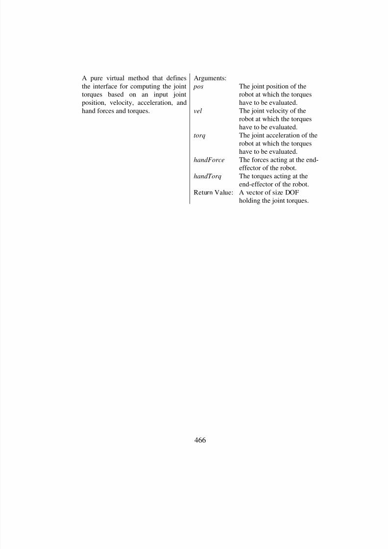
8/3/2019 Chetan Kapoor Dissertation
http://slidepdf.com/reader/full/chetan-kapoor-dissertation 487/612
466
A pure virtual method that definesthe interface for computing the joint
torques based on an input jointposition, velocity, acceleration, andhand forces and torques.
Arguments:
pos The joint position of the
robot at which the torqueshave to be evaluated.
vel The joint velocity of therobot at which the torqueshave to be evaluated.
torq The joint acceleration of therobot at which the torqueshave to be evaluated.
handForce The forces acting at the end-effector of the robot.
handTorq The torques acting at theend-effector of the robot.
Return Value: A vector of size DOFholding the joint torques.

8/3/2019 Chetan Kapoor Dissertation
http://slidepdf.com/reader/full/chetan-kapoor-dissertation 488/612
467
B.7.2. class RRIDNewtonEuler : public RRInverseDynamics.hpp
#include <InverseDynamics/InverseDynamics.hpp>
Public Methods
RRIDNewtonEuler(const RRString& DHfile, const RRString& linkCGM, constRRString& linkInerita, const RRVector3D& gravity = RRVector3D(0.0, 0.0, 9.8));
Constructor. This class implementsthe recursive Newton-Euler inversedynamics technique.
Arguments:
DHfile File containing the Denavit-Hartenberg parameters of the robot in question.
linkCGM File whose each rowcontains the location of the
center-of-gravity and massof each link. The center-of-gravity is expressed in ‘X’,‘Y’, and ‘Z’ coordinates of the local link frames. Thenumber of rows in this filesshould be equal to the DOFof the robot.
linkInertia File containing the inertia’sof each link expressed intheir local coordinateframes. Inertia for each link
is expressed as a 3 X 3matrix (or an inertia tensor).The number of inertiatensors in this file should beequal to the DOF of therobot.
gravity The acceleration due togravity expressed in thebase coordinate frame of therobot.
~RRIDNewtonEuler();
Destructor. Deallocates memory.
const RRVector& GetJointTorques( const RRVector& pos, const RRVector& vel,const RRVector& acc, const RRVector3D& handForce, const RRVector3D&handTorque);

8/3/2019 Chetan Kapoor Dissertation
http://slidepdf.com/reader/full/chetan-kapoor-dissertation 489/612
468
This method implements thefunctionality for computing the
inverse dynamics solution using therecursive Newton-Euler technique.
Arguments:
pos The joint position of the
robot at which the torqueshave to be evaluated.
vel The joint velocity of therobot at which the torqueshave to be evaluated.
torq The joint acceleration of therobot at which the torqueshave to be evaluated.
handForce The forces acting at the end-effector of the robot.
handTorq The torques acting at theend-effector of the robot.
Return Value: A vector of size DOFholding the joint torques.
void SetToolPoint(const RRVector3D& toolPoint);
This method is used to set the valueof the tool point vector (x,y,z)specified in the coordinate frameattached to the last link. If thismethod is not called, the tool pointvector is considered to be [0, 0, 0].
Arguments:toolPoint The vector holding the X,
Y, and Z coordinates of thetool point.
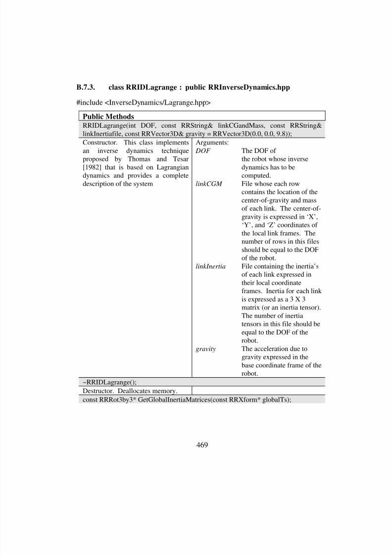
8/3/2019 Chetan Kapoor Dissertation
http://slidepdf.com/reader/full/chetan-kapoor-dissertation 490/612
469
B.7.3. class RRIDLagrange : public RRInverseDynamics.hpp
#include <InverseDynamics/Lagrange.hpp>
Public Methods
RRIDLagrange(int DOF, const RRString& linkCGandMass, const RRString&linkInertiafile, const RRVector3D& gravity = RRVector3D(0.0, 0.0, 9.8));
Constructor. This class implementsan inverse dynamics techniqueproposed by Thomas and Tesar[1982] that is based on Lagrangiandynamics and provides a completedescription of the system
Arguments:
DOF The DOF of the robot whose inversedynamics has to becomputed.
linkCGM File whose each row
contains the location of thecenter-of-gravity and massof each link. The center-of-gravity is expressed in ‘X’,‘Y’, and ‘Z’ coordinates of the local link frames. Thenumber of rows in this filesshould be equal to the DOFof the robot.
linkInertia File containing the inertia’sof each link expressed intheir local coordinate
frames. Inertia for each link is expressed as a 3 X 3matrix (or an inertia tensor).The number of inertiatensors in this file should beequal to the DOF of therobot.
gravity The acceleration due togravity expressed in thebase coordinate frame of therobot.
~RRIDLagrange();
Destructor. Deallocates memory.const RRRot3by3* GetGlobalInertiaMatrices(const RRXform* globalTs);

8/3/2019 Chetan Kapoor Dissertation
http://slidepdf.com/reader/full/chetan-kapoor-dissertation 491/612
470
This method computes the inertiamatrices of each link with respect to
the base frame of the robot. Thelocal inertia matrices were read infrom a data file during objectcreation.
Arguments:
globalTs An array of global
transformation matrices of the links of the robot. Thesize of this array should beequal to DOF.
Return Value: A pointer to an array of 3 X3 matrices of size DOF thatcontain the global inertiamatrices of the links of therobot.
const RRMatrix* GetIstar(const RRTensor& rotGfunc, const RRTensor&transGfunc);
This method is used to compute the
effective inertia of the system. Thismethod should be called after asuccessful call toGetGlobalInertiaMatrices
Arguments:
rotGfunc A tensor of size 3X3XDOFthat holds the rotational firstorder influence coefficientsof the robot at the desired joint position for whichIstar has to be computed.
transGfunc A tensor of size 3X3XDOFthat holds the translationalfirst-order influencecoefficients of the robot atthe desired joint position forwhich Istar has to be
computed. Thesecoefficients should becomputed for the center of mass of each link.
Return Value: A matrix of size DOF XDOF that contains theeffective inertia of thesystem.
const RRMatrix* GetIstar(const RRXform* globalTs, const RRTensor& rotGfunc,const RRTensor& transGfunc);

8/3/2019 Chetan Kapoor Dissertation
http://slidepdf.com/reader/full/chetan-kapoor-dissertation 492/612
471
This method is used to compute theeffective inertia of the system. This
method does not have to be calledafter a call toGetGlobalInertiaMatrices as theglobalTs argument is used to updatethe global inertia matrices.
Arguments:
globalTs An array of global
transformation matrices of the links of the robot. Thesize of this array should beequal to DOF.
rotGfunc A tensor of size 3X3XDOFthat holds the rotational firstorder influence coefficientsof the robot at the desired joint position for whichIstar has to be computed.
transGfunc A tensor of size 3X3XDOFthat holds the translational
first-order influencecoefficients of the robot atthe desired joint position forwhich Istar has to becomputed. Thesecoefficients should becomputed for the center of mass of each link.
Return Value: A matrix of size DOF XDOF that contains theeffective inertia of thesystem.
const RRTensor* GetPstar(const RRTensor& rotGfunc, const RRTensor&transGfunc, const RRTensor** rotHfunc, const RRTensor** transHfunc);
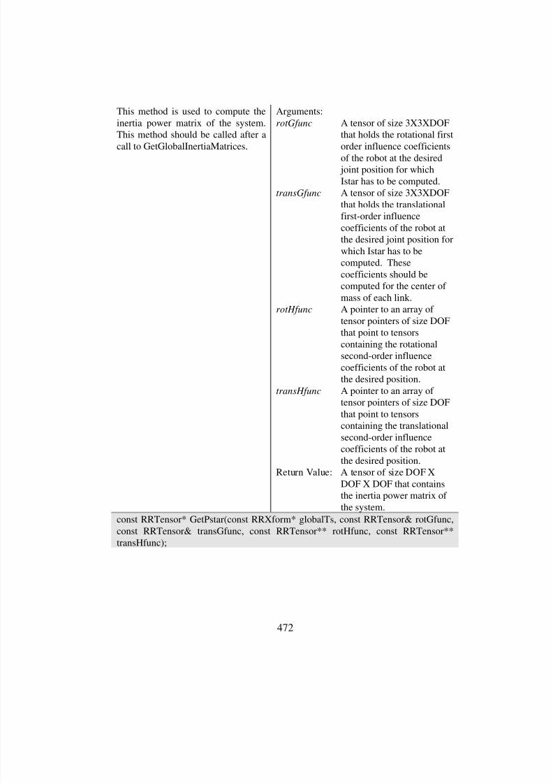
8/3/2019 Chetan Kapoor Dissertation
http://slidepdf.com/reader/full/chetan-kapoor-dissertation 493/612
472
This method is used to compute theinertia power matrix of the system.
This method should be called after acall to GetGlobalInertiaMatrices.
Arguments:
rotGfunc A tensor of size 3X3XDOF
that holds the rotational firstorder influence coefficientsof the robot at the desired joint position for whichIstar has to be computed.
transGfunc A tensor of size 3X3XDOFthat holds the translationalfirst-order influencecoefficients of the robot atthe desired joint position forwhich Istar has to becomputed. These
coefficients should becomputed for the center of mass of each link.
rotHfunc A pointer to an array of tensor pointers of size DOFthat point to tensorscontaining the rotationalsecond-order influencecoefficients of the robot atthe desired position.
transHfunc A pointer to an array of tensor pointers of size DOF
that point to tensorscontaining the translationalsecond-order influencecoefficients of the robot atthe desired position.
Return Value: A tensor of size DOF XDOF X DOF that containsthe inertia power matrix of the system.
const RRTensor* GetPstar(const RRXform* globalTs, const RRTensor& rotGfunc,const RRTensor& transGfunc, const RRTensor** rotHfunc, const RRTensor**transHfunc);
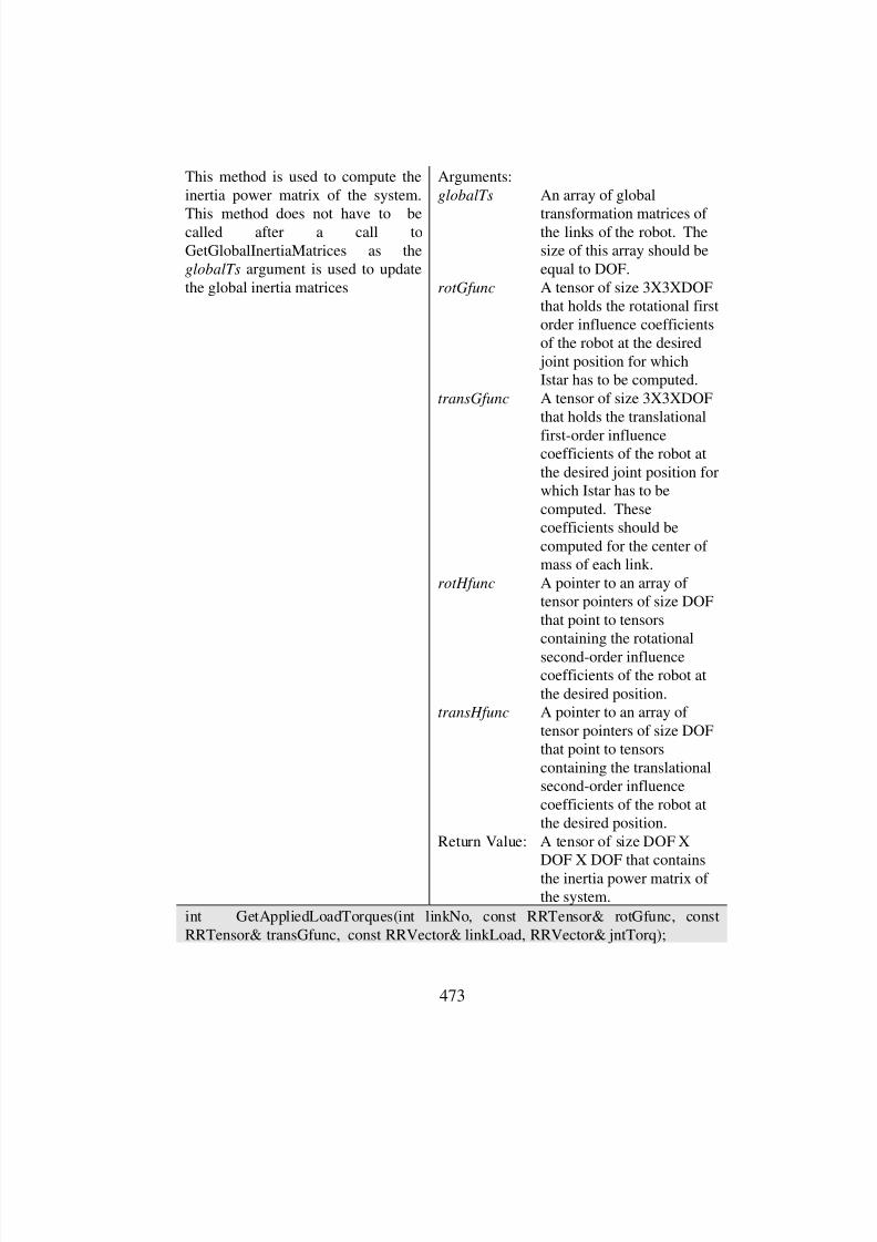
8/3/2019 Chetan Kapoor Dissertation
http://slidepdf.com/reader/full/chetan-kapoor-dissertation 494/612
473
This method is used to compute theinertia power matrix of the system.
This method does not have to becalled after a call toGetGlobalInertiaMatrices as theglobalTs argument is used to updatethe global inertia matrices
Arguments:
globalTs An array of global
transformation matrices of the links of the robot. Thesize of this array should beequal to DOF.
rotGfunc A tensor of size 3X3XDOFthat holds the rotational firstorder influence coefficientsof the robot at the desired joint position for whichIstar has to be computed.
transGfunc A tensor of size 3X3XDOFthat holds the translational
first-order influencecoefficients of the robot atthe desired joint position forwhich Istar has to becomputed. Thesecoefficients should becomputed for the center of mass of each link.
rotHfunc A pointer to an array of tensor pointers of size DOFthat point to tensorscontaining the rotational
second-order influencecoefficients of the robot atthe desired position.
transHfunc A pointer to an array of tensor pointers of size DOFthat point to tensorscontaining the translationalsecond-order influencecoefficients of the robot atthe desired position.
Return Value: A tensor of size DOF XDOF X DOF that containsthe inertia power matrix of the system.
int GetAppliedLoadTorques(int linkNo, const RRTensor& rotGfunc, constRRTensor& transGfunc, const RRVector& linkLoad, RRVector& jntTorq);
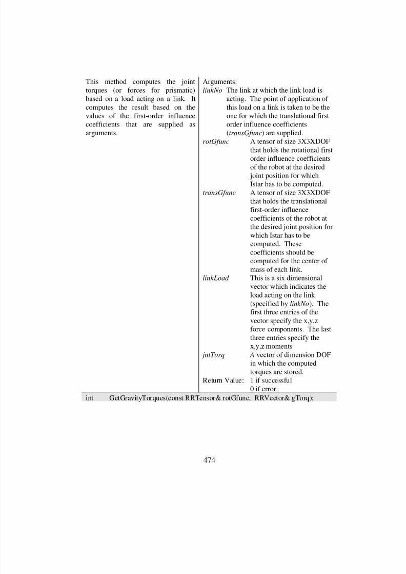
8/3/2019 Chetan Kapoor Dissertation
http://slidepdf.com/reader/full/chetan-kapoor-dissertation 495/612
474
This method computes the jointtorques (or forces for prismatic)
based on a load acting on a link. Itcomputes the result based on thevalues of the first-order influencecoefficients that are supplied asarguments.
Arguments:
linkNo The link at which the link load is
acting. The point of application of this load on a link is taken to be theone for which the translational firstorder influence coefficients(transGfunc) are supplied.
rotGfunc A tensor of size 3X3XDOFthat holds the rotational firstorder influence coefficientsof the robot at the desired joint position for whichIstar has to be computed.
transGfunc A tensor of size 3X3XDOF
that holds the translationalfirst-order influencecoefficients of the robot atthe desired joint position forwhich Istar has to becomputed. Thesecoefficients should becomputed for the center of mass of each link.
linkLoad This is a six dimensionalvector which indicates theload acting on the link
(specified by linkNo). Thefirst three entries of thevector specify the x,y,zforce components. The lastthree entries specify thex,y,z moments
jntTorq A vector of dimension DOFin which the computedtorques are stored.
Return Value: 1 if successful0 if error.
int GetGravityTorques(const RRTensor& rotGfunc, RRVector& gTorq);
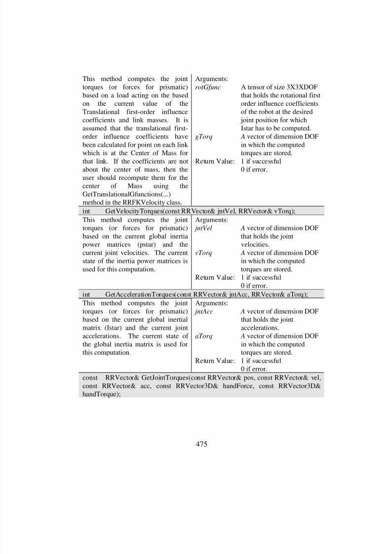
8/3/2019 Chetan Kapoor Dissertation
http://slidepdf.com/reader/full/chetan-kapoor-dissertation 496/612
475
This method computes the jointtorques (or forces for prismatic)
based on a load acting on the basedon the current value of theTranslational first-order influencecoefficients and link masses. It isassumed that the translational first-order influence coefficients havebeen calculated for point on each link which is at the Center of Mass forthat link. If the coefficients are notabout the center of mass, then theuser should recompute them for thecenter of Mass using the
GetTranslationalGfunctions(...)method in the RRFKVelocity class.
Arguments:
rotGfunc A tensor of size 3X3XDOF
that holds the rotational firstorder influence coefficientsof the robot at the desired joint position for whichIstar has to be computed.
gTorq A vector of dimension DOFin which the computedtorques are stored.
Return Value: 1 if successful0 if error.
int GetVelocityTorques(const RRVector& jntVel, RRVector& vTorq);
This method computes the jointtorques (or forces for prismatic)based on the current global inertiapower matrices (pstar) and thecurrent joint velocities. The currentstate of the inertia power matrices isused for this computation.
Arguments: jntVel A vector of dimension DOF
that holds the jointvelocities.
vTorq A vector of dimension DOFin which the computedtorques are stored.
Return Value: 1 if successful0 if error.
int GetAccelerationTorques(const RRVector& jntAcc, RRVector& aTorq);
This method computes the jointtorques (or forces for prismatic)based on the current global inertialmatrix (Istar) and the current jointaccelerations. The current state of the global inertia matrix is used forthis computation.
Arguments:
jntAcc A vector of dimension DOFthat holds the jointaccelerations.
aTorq A vector of dimension DOFin which the computedtorques are stored.
Return Value: 1 if successful0 if error.
const RRVector& GetJointTorques(const RRVector& pos, const RRVector& vel,
const RRVector& acc, const RRVector3D& handForce, const RRVector3D&handTorque);
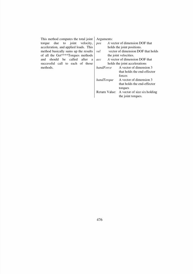
8/3/2019 Chetan Kapoor Dissertation
http://slidepdf.com/reader/full/chetan-kapoor-dissertation 497/612
476
This method computes the total jointtorque due to joint velocity,
acceleration, and applied loads. Thismethod basically sums up the resultsof all the Get****Torques methodsand should be called after asuccessful call to each of thosemethods.
Arguments:
pos A vector of dimension DOF that
holds the joint positions.vel vector of dimension DOF that holds
the joint velocities.
acc A vector of dimension DOF thatholds the joint accelerations
handForce A vector of dimension 3that holds the end-effectorforces
handTorque A vector of dimension 3that holds the end-effectortorques
Return Value: A vector of size six holding
the joint torques.
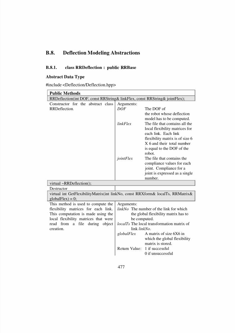
8/3/2019 Chetan Kapoor Dissertation
http://slidepdf.com/reader/full/chetan-kapoor-dissertation 498/612
477
B.8. Deflection Modeling Abstractions
B.8.1. class RRDeflection : public RRBase
Abstract Data Type
#include <Deflection/Deflection.hpp>
Public Methods
RRDeflection(int DOF, const RRString& linkFlex, const RRString& jointFlex);
Constructor for the abstract classRRDeflection.
Arguments: DOF The DOF of
the robot whose deflectionmodel has to be computed.
linkFlex The file that contains all thelocal flexibility matrices foreach link. Each link flexibility matrix is of size 6X 6 and their total numberis equal to the DOF of therobot.
jointFlex The file that contains thecompliance values for each joint. Compliance for a
joint is expressed as a singlenumber.
virtual ~RRDeflection();
Destructor
virtual int GetFlexibilityMatrix(int linkNo, const RRXform& localTs, RRMatrix&globalFlex) = 0;
This method is used to compute theflexibility matrices for each link.This computation is made using thelocal flexibility matrices that wereread from a file during objectcreation.
Arguments:
linkNo The number of the link for whichthe global flexibility matrix has tobe computed.
localTs The local transformation matrix of link linkNo.
globalFlex A matrix of size 6X6 inwhich the global flexibilitymatrix is stored.
Return Value: 1 if successful0 if unsuccessful
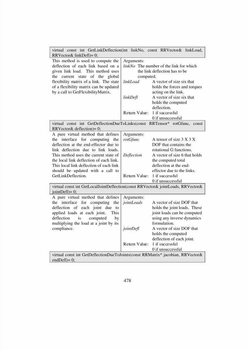
8/3/2019 Chetan Kapoor Dissertation
http://slidepdf.com/reader/full/chetan-kapoor-dissertation 499/612
478
virtual const int GetLinkDeflection(int linkNo, const RRVector& linkLoad,RRVector& linkDefl)= 0;
This method is used to compute thedeflection of each link based on agiven link load. This method usesthe current state of the globalflexibility matrix of a link. The stateof a flexibility matrix can be updatedby a call to GetFlexibilityMatrix.
Arguments:linkNo The number of the link for which
the link deflection has to becomputed.
linkLoad A vector of size six thatholds the forces and torquesacting on the link.
linkDefl A vector of size six thatholds the computeddeflection.
Return Value: 1 if successful0 if unsuccessful
virtual const int GetDeflectionDueToLinks(const RRTensor* rotGfunc, constRRVector& deflection)= 0;
A pure virtual method that definesthe interface for computing thedeflection at the end-effector due tolink deflection due to link loads.This method uses the current state of the local link deflection of each link.This local link deflection of each link should be updated with a call toGetLinkDeflection.
Arguments:rotGfunc A tensor of size 3 X 3 X
DOF that contains therotational G functions.
Deflection A vector of size 6 that holdsthe computed totaldeflection at the end-effector due to the links.
Return Value: 1 if successful0 if unsuccessful
virtual const int GetLocalJointDeflection(const RRVector& jointLoads, RRVector& jointDefl)= 0;
A pure virtual method that definesthe interface for computing thedeflection of each joint due toapplied loads at each joint. Thisdeflection is computed bymultiplying the load at a joint by itscompliance.
Arguments:
jointLoads A vector of size DOF thatholds the joint loads. These joint loads can be computedusing any inverse dynamicsformulation.
jointDefl A vector of size DOF thatholds the computeddeflection of each joint.
Return Value: 1 if successful0 if unsuccessful
virtual const int GetDeflectionDueToJoints(const RRMatrix* jacobian, RRVector&endDefl)= 0;

8/3/2019 Chetan Kapoor Dissertation
http://slidepdf.com/reader/full/chetan-kapoor-dissertation 500/612
479
A pure virtual method that definesthe interface for computing the
deflection at the end-effector due todeflections at the joints. Thismethod uses the current state of the joint deflections to compute thedeflection at the end-effector. TheJacobian supplied to this methodshould have been computed for the joint position at which the deflectionis being computed.
Arguments:
jacobian A matrix of size 6 X DOF
that contains the Jacobianfor matrix for the end-effector.
endDefl A vector of size 6 that holdsthe computed totaldeflection at the end-effector due to the joints.
Return Value: 1 if successful0 if unsuccessful
virtual const int GetDeflectionDueToJoints(const RRMatrix* jacobian, constRRVector& jointLoads, RRVector& endDefl)= 0;
A pure virtual method that defines
the interface for computing thedeflection at the end-effector due todeflections at the joints. Thismethod first callsGetLocalJointDeflection to computethe deflection at each joint. TheJacobian supplied to this methodshould have been computed for the joint position at which the deflectionis being computed.
Arguments:
jacobian A matrix of size 6 X DOFthat contains the Jacobianfor matrix for the end-effector.
jointLoads A vector of size DOF thatholds the joint loads. These joint loads can be computedusing any inverse dynamicsformulation.
endDefl A vector of size 6 that holdsthe computed deflection of the end-effector.
Return Value: 1 if successful0 if unsuccessful

8/3/2019 Chetan Kapoor Dissertation
http://slidepdf.com/reader/full/chetan-kapoor-dissertation 501/612
480
B.9. IODevices Abstractions
B.9.1. class RRKeyboard : public RRBase
#include <IODevices/Keyboard.hpp>
Public Data Members
enum BLOCKMODE {NONBLOCK = 0, BLOCK = 1};
This enumeration defines a data type that can be used for setting the state of akeyboard. If the BLOCKMODE is NONBLOCK, the keyboard can be readasynchronously. That is the program will not wait for a key to be pressed. If theBLOCKMODE is BLOCK, the program will wait till a key is pressed.
Public MethodsRRKeyboard(BLOCKMODE blockMode = BLOCK);
Constructor. The blocking mode isset to BLOCK by default.
Arguments:
blockMode Specify the blocking statusof the keyboard.
~RRKeyboard();
Destructor. Resets the state of thekeyboard to canonical processing of characters.
int GetKeyState(char key);
This method gets the state of aparticular key specified by key.
Arguments:key The key whose sates is desired.Return Value: 1 if key is pressed
0 if key is not pressed
char GetKey(void);
This method returns the key that ispressed. In block mode, this methodwaits till a key is pressed and in non-block it just polls.
Return Value: The key that is pressed.0 if no key is pressed (inNONBLOCK mode)
int SetBlockingMode(enum BLOCKMODE blockMode);
This method sets the blocking modeof the keyboard.
Arguments:blockMode The desired blocking modeReturn Value: 1 if successful
0 if unsuccessfulBLOCKMODE GetBlockMode(void);
This method gets the blocking modeof the keyboard.
Return Value: the BLOCKMODE
int UpdateVector(RRVector& input, const RRVector& deltas, char quitKey =ESC);
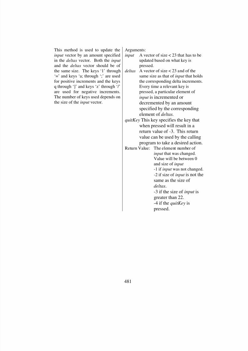
8/3/2019 Chetan Kapoor Dissertation
http://slidepdf.com/reader/full/chetan-kapoor-dissertation 502/612
481
This method is used to update the
input vector by an amount specified
in the deltas vector. Both the input and the deltas vector should be of the same size. The keys ‘1’ through‘=’ and keys ‘a; through ‘;’ are usedfor positive increments and the keysq through ‘]’ and keys ‘z’ through ‘/’are used for negative increments.The number of keys used depends onthe size of the input vector.
Arguments:
input A vector of size < 23 that has to be
updated based on what key ispressed.
deltas A vector of size < 23 and of thesame size as that of input that holdsthe corresponding delta increments.Every time a relevant key ispressed, a particular element of
input is incremented ordecremented by an amount
specified by the correspondingelement of deltas.
quitKey This key specifies the key that
when pressed will result in areturn value of -3. This returnvalue can be used by the calling
program to take a desired action.Return Value: The element number of
input that was changed.Value will be between 0and size of input
-1 if input was not changed.
-2 if size of input is not thesame as the size of
deltas.-3 if the size of input isgreater than 22.-4 if the quitKey is
pressed.

8/3/2019 Chetan Kapoor Dissertation
http://slidepdf.com/reader/full/chetan-kapoor-dissertation 503/612
482
B.10. Controller Abstractions
B.10.1. class RRController : public RRBase
Abstract Data Type
#include <Controller/Controller.hpp>
Public Methods
RRController(const RRString& name);
Constructor. This is the constructorfor this abstract class that defines theinterface for all manual controllers.Interface declaration has yet to beprovided for this class.
Arguments:
name Name of the object.
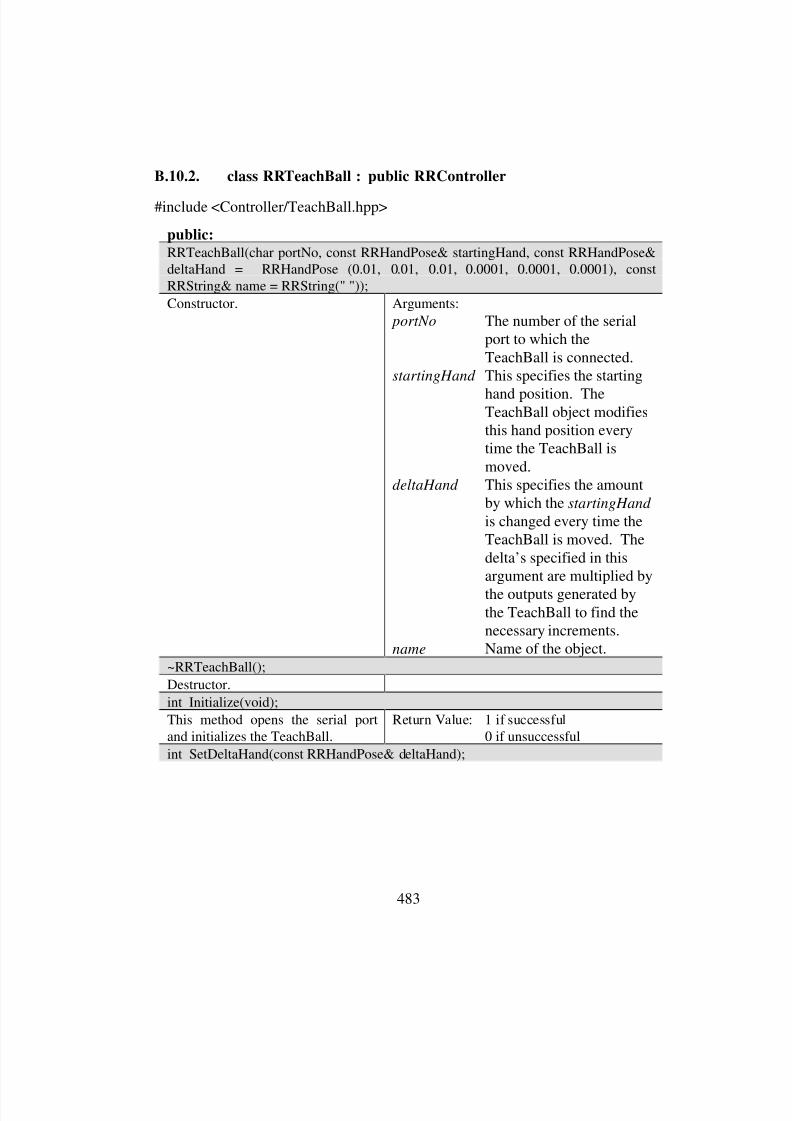
8/3/2019 Chetan Kapoor Dissertation
http://slidepdf.com/reader/full/chetan-kapoor-dissertation 504/612
483
B.10.2. class RRTeachBall : public RRController
#include <Controller/TeachBall.hpp>
public:
RRTeachBall(char portNo, const RRHandPose& startingHand, const RRHandPose&deltaHand = RRHandPose (0.01, 0.01, 0.01, 0.0001, 0.0001, 0.0001), constRRString& name = RRString(" "));
Constructor. Arguments:
portNo The number of the serialport to which the
TeachBall is connected.startingHand This specifies the starting
hand position. TheTeachBall object modifiesthis hand position everytime the TeachBall is
moved.deltaHand This specifies the amount
by which the startingHand
is changed every time theTeachBall is moved. The
delta’s specified in thisargument are multiplied by
the outputs generated bythe TeachBall to find thenecessary increments.
name Name of the object.~RRTeachBall();
Destructor.
int Initialize(void);
This method opens the serial portand initializes the TeachBall.
Return Value: 1 if successful0 if unsuccessful
int SetDeltaHand(const RRHandPose& deltaHand);
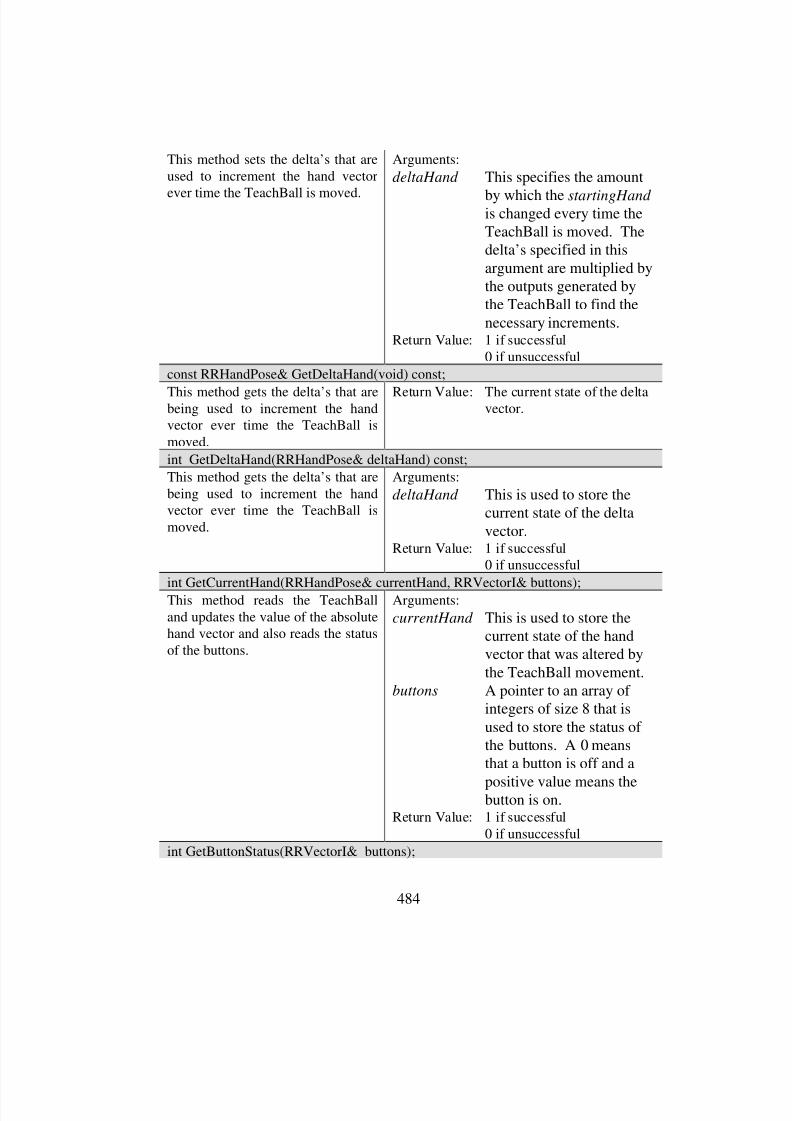
8/3/2019 Chetan Kapoor Dissertation
http://slidepdf.com/reader/full/chetan-kapoor-dissertation 505/612
484
This method sets the delta’s that areused to increment the hand vector
ever time the TeachBall is moved.
Arguments:
deltaHand This specifies the amount
by which the startingHand is changed every time theTeachBall is moved. Thedelta’s specified in this
argument are multiplied bythe outputs generated bythe TeachBall to find the
necessary increments.Return Value: 1 if successful
0 if unsuccessful
const RRHandPose& GetDeltaHand(void) const;
This method gets the delta’s that arebeing used to increment the handvector ever time the TeachBall ismoved.
Return Value: The current state of the deltavector.
int GetDeltaHand(RRHandPose& deltaHand) const;
This method gets the delta’s that arebeing used to increment the handvector ever time the TeachBall ismoved.
Arguments:
deltaHand This is used to store thecurrent state of the delta
vector.Return Value: 1 if successful
0 if unsuccessful
int GetCurrentHand(RRHandPose& currentHand, RRVectorI& buttons);This method reads the TeachBalland updates the value of the absolutehand vector and also reads the statusof the buttons.
Arguments:
currentHand This is used to store thecurrent state of the handvector that was altered by
the TeachBall movement.buttons A pointer to an array of
integers of size 8 that is
used to store the status of the buttons. A 0 meansthat a button is off and a
positive value means thebutton is on.
Return Value: 1 if successful0 if unsuccessful
int GetButtonStatus(RRVectorI& buttons);

8/3/2019 Chetan Kapoor Dissertation
http://slidepdf.com/reader/full/chetan-kapoor-dissertation 506/612
485
This method reads the TeachBalland updates the status of the buttons.
Arguments:
buttons A pointer to an array of
integers of size 8 that isused to store the status of the buttons. A 0 meansthat a button is off and a
positive value means thebutton is on.
Return Value: 1 if successful0 if unsuccessful
int SetCurrentHand(RRHandPose& currentHand);
This method sets the value of thecurrent hand. This new value of the
current hand is the one that getsaltered every time the TeachBall ismoved. Using this method theTeachBall can be multiplexed tocontrol different devices.
Arguments:
currentHand This argument sets the state
of the current hand.Return Value: 1 if successful
0 if unsuccessful
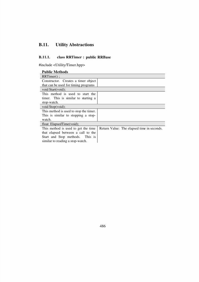
8/3/2019 Chetan Kapoor Dissertation
http://slidepdf.com/reader/full/chetan-kapoor-dissertation 507/612
486
B.11. Utility Abstractions
B.11.1. class RRTimer : public RRBase
#include <Utility/Timer.hpp>
Public Methods
RRTimer() ;
Constructor. Creates a timer objectthat can be used for timing programs
void Start(void);
This method is used to start the
timer. This is similar to starting astop-watch.
void Stop(void);
This method is used to stop the timer.This is similar to stopping a stop-watch.
float ElapsedTime(void);
This method is used to get the timethat elapsed between a call to theStart and Stop methods. This issimilar to reading a stop-watch.
Return Value: The elapsed time in seconds.
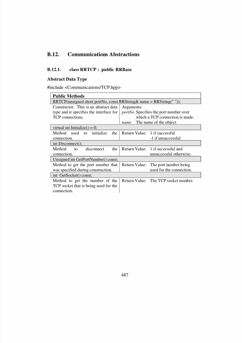
8/3/2019 Chetan Kapoor Dissertation
http://slidepdf.com/reader/full/chetan-kapoor-dissertation 508/612
487
B.12. Communications Abstractions
B.12.1. class RRTCP : public RRBase
Abstract Data Type
#include <Communications/TCP.hpp>
Public Methods
RRTCP(unsigned short portNo, const RRString& name = RRString(" "));
Constructor. This is an abstract datatype and it specifies the interface forTCP connections.
Arguments: portNo Specifies the port number over
which a TCP connection is made.name The name of the object.
virtual int Initialize() = 0;
Method used to initialize theconnection.
Return Value: 1 if successful-1 if unsuccessful
int Disconnect();
Method to disconnect theconnection.
Return Value: 1 if successful andunsuccessful otherwise.
Unsigned int GetPortNumber() const;
Method to get the port number thatwas specified during construction.
Return Value: The port number beingused for the connection.
int GetSocket() const;
Method to get the number of theTCP socket that is being used for theconnection.
Return Value: The TCP socket number.

8/3/2019 Chetan Kapoor Dissertation
http://slidepdf.com/reader/full/chetan-kapoor-dissertation 509/612
488
B.12.2. class RRTCPClient : public RRTCP
#include <Communications/TCP.hpp>
Public Methods
RRTCPClient(unsigned short portNo, const RRString& destIP, const RRString&name = RRString(" "));
Constructor. This class is used forcreating a TCP client. The TCPclient initiates communication with aTCP server by connecting to it.
Arguments:
portNo Specifies the port number overwhich a TCP connection is made.
destIP The Internet protocol address of thecompute on which the server towhich the connection to be made is
running.name The name of the object.
int Initialize();
Method used to make the connectionwith the server
Return Value: 1 if successful-1 if unsuccessful
int Transmit(char* data, unsigned int length);
Method used to transmit data to theserver. When data is transmittedusing this method, a reply is notexpected from the server.
Arguments:
data A pointer to the data that has to betransmitted.
length The length in bytes of the data thathas to be transmitted.
Return Value: Number of bytes transmitted
-1 if unsuccessfulint Transmit(char* sendData, unsigned int sendLength, char* recvData, unsigned intrecvLength);
Method used to transmit data to theserver. When data is transmittedusing this method, a reply is expectedfrom the server.
Arguments:sendData A pointer to the data that
has to be transmitted.sendLength The length in bytes of the
data that has to betransmitted.
recvData A pointer to a characterarray in which the receiveddata has to be stored.
recvLength The length of the data to bereceived.
Return Value: Number of bytes transmitted0 if unsuccessful

8/3/2019 Chetan Kapoor Dissertation
http://slidepdf.com/reader/full/chetan-kapoor-dissertation 510/612
489
B.12.3. class RRTCPServer : public RRTCP
#include <Communications/TCP.hpp>
Public Methods
RRTCPServer(unsigned short portNo, const RRString& name = RRString(" "));
Constructor. This class is used forcreating a TCP server. The TCPserver waits and listens till a clientconnects to it.
Arguments: portNo Specifies the port number over
which a TCP connection is made.name The name of the object.
int Disconnect();
Method to disconnect the connection. Return Value: 1 if successful andunsuccessful otherwise.
int Initialize();Method used to wait and listen till aclient connects.
Return Value: 1 if successful-1 if unsuccessful
int Receive(char* recvData, unsigned int recvLength);
Method used to receive data from theclient.
Arguments:recvData A pointer to an array in
which the received data is tobe stored.
recvLength The length in bytes of thedata that has to be received.
Return Value: Number of bytes received-1 if unsuccessful
int Reply(char* sendData, unsigned int sendLength);Method used to send a reply to theclient.
Arguments:
sendData A pointer to the data thathas to be sent to the client.
sendLength The length in bytes of thedata that has to be sent.
Return Value: Number of bytes sent-1 if unsuccessful

8/3/2019 Chetan Kapoor Dissertation
http://slidepdf.com/reader/full/chetan-kapoor-dissertation 511/612
490
Appendix C
C. Experiments with OSCAR
C.1. Proposed Test Activity
This paper proposes a means of testing the object-oriented software
components being developed at the Robotics Research Group as a part of this
dissertation. The purpose of this activity is two-fold. First, this activity will
provide an environment that will be useful in debugging the software components,
testing their reuse and rapid-prototyping potential, and also realizing their worth
for real-world applications. The second benefit of this activity is that it will
expose future users of the software components to the application domain and
usage of the software. Users will gain information regarding what is available,
where it is available, how to use it, how to get maximum software reuse, and how
to achieve rapid-prototyping with these components. In addition, the users will be
exposed to the development environment (operating system, makefiles, source
code control, editors, and software development guidelines(see Appendix A))[
Silberschatz and Gahin, 1994] [Oram and Talbott, 1995] [Bolinger and Bronson,1995]. This information is imperative to any world class software development.
8/3/2019 Chetan Kapoor Dissertation
http://slidepdf.com/reader/full/chetan-kapoor-dissertation 512/612
491
C.2. Desired User Qualifications
There are two areas in which the user has to be proficient. First, the user
should be well versed in object-oriented design and the C++ programming
language. Knowledge about operating systems, parallel execution environments,
and source code management is desired but not needed. Second, the user should
understand the domain of advanced robotics. This includes linear algebra,
generalized kinematics (both forward and inverse), generalized dynamics,
generalized deflection modeling, and performance criteria. In depth
understanding of the domains is not needed, though the key inputs and outputs of each domain should be well understood. A complete understanding of the domain
will be needed if the user intends to add additional functionality to the existing
software components. Most of all, the user should exhibit sound engineering and
design skills. Here are a few suggestions that are necessary to develop reusable
software components:
Be well versed in the C++ programming language and object-oriented design.
Implementation should be less of a challenge. The challenge should be in the
domain analysis and the conceptual design.
When tackling a problem, do not start worrying about implementation details
till you have worked out an analytical design solution.
Think of software components independently of each other. This will let you
design better reusable software classes.
Software components should not be designed for use in a particular
application. For every component think of all possible use-case scenarios and
future reusability support.
While implementing, try to provide two interfaces to each class. The first
interface should be targeted for ease of use while the second should be

8/3/2019 Chetan Kapoor Dissertation
http://slidepdf.com/reader/full/chetan-kapoor-dissertation 513/612
492
targeted at maximum computational efficiency. For example, consider the
Matrix class in which the operator * is overloaded for Matrix multiplication.
This method leads to a constructor call that is used to return the product of
two matrices (most compilers will optimize here, but still….). As most
robotics software is executed repeatedly in a loop, it will be beneficial to
provide another interface for multiplying two Matrices. This interface will
eliminate the allocation of Matrix object every time two matrices are
multiplied.
C.3. Software Development Environment
The software development environment has three main components.
These are explained below:
C.3.1. Programming Language
The programming language of choice is C++. Two compilers are
available for source code compiling. The first is the Sun C++ compiler that can
be used to generate executables for the Solaris operating system. Theseexecutables execute on a SUN workstation running Solaris 2.2. The other
available compiler is the GNU C++ cross-compiler for the Motorola 68k family of
processors and the VxWorks operating system from Wind River Systems
[WindRiver Systems, VxWorks Programmer’s Guide]. As the GNU compiler is a
cross-compiler, it is used on the SUN workstation to produce machine code that
can be downloaded to a 68k processor running VxWorks 5.2. Both these
compilers support parameterized data-types (templates) but use different
techniques for template instantiations. The VxWorks development environment
also supports the Tools.h++ library from RogueWave software, the iostreams
libraries from AT&T and the Booch components [RogueWave Software, C++
8/3/2019 Chetan Kapoor Dissertation
http://slidepdf.com/reader/full/chetan-kapoor-dissertation 514/612
493
Booch Components] [RogueWave Software, Tools.h++]. The Sun C++ compiler
supports iostreams libraries.
C.3.2. Operating Systems
Source code can be currently compiled using the compilers mentioned
above for the Solaris (using SUN C++) operating system and for VxWorks using
the GNU C++ compiler. The majority of the source code compiles for both
operating systems. Almost all the I/O interfacing code is specific to the VxWorks
operating system and does not compile under Solaris. Applications can be
developed to control either a graphical simulation or a physical robot.
Applications developed for VxWorks can be used for both these purposes
whereas applications developed on the SUN can only be used to control a
simulation.
C.3.3. Source Code Organization
Currently all the source code is placed in the ‘oscar’ account on the SUN
workstation (darkstar.mer.utexas.edu). The source code is organized in differentdirectories based on the domain it belongs to. The absolute path to the source
code is “/export/home/oscar/Research/src.” Under ‘src’ the domains are
partitioned into different directories. This directory structure is graphically shown
in Figure C.1 and a brief description of the directories is listed.
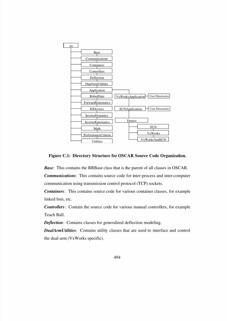
8/3/2019 Chetan Kapoor Dissertation
http://slidepdf.com/reader/full/chetan-kapoor-dissertation 515/612
494
src
Communications
Base
Containers
Deflection
Controllers
RobotData
DualArmUtilities
ForwardKinematics
InverseDynamics
IODevices
Math
InverseKinematics
PerformanceCriteria
Utilities
Application
SUNApplication
Demos
VxWorks
SUN
VxWorksAndSUN
VxWorksApplication User Directories
User Directories
Figure C.1: Directory Structure for OSCAR Source Code Organization.
Base: This contains the RRBase class that is the parent of all classes in OSCAR.Communications: This contains source code for inter-process and inter-computer
communication using transmission control protocol (TCP) sockets.
Containers: This contains source code for various container classes, for example
linked lists, etc.
Controllers: Contain the source code for various manual controllers, for example
Teach Ball.
Deflection: Contains classes for generalized deflection modeling.
DualArmUtilities: Contains utility classes that are used to interface and control
the dual-arm (VxWorks specific).
8/3/2019 Chetan Kapoor Dissertation
http://slidepdf.com/reader/full/chetan-kapoor-dissertation 516/612
495
RobotData: Contains classes for reading formatted data from files. For example,
DH parameter data.
ForwardKinematics: Contains classes for generalized forward kinematics.
IODevices: Contains classes for various IO devices like serial ports (VxWorks
specific).
InverseDynamics: Contains classes for generalized inverse dynamics of serial
robots.
InverseKinematics: Contains classes for generalized inverse kinematics for serial
robots.
Math: Contains classes for various linear algebra constructs, for example
matrices, vectors, tensors, etc.
PerformanceCriteria: Contains classes for performance criteria and criteria
fusion.
Utilities: Contains source code for utility data types (string) and error checking
source code.
Application: This is the directory in which a user can create and compile an
application that uses OSCAR. Individual sub-directories should be created by
users for better organization.
SUNApplication: This directory should be used to create Solaris specific
applications. Users should create personal directories inside this directory for
their Solaris specific applications.
VxWorksApplication: This directory should be used to create VxWorks specific
applications. Users should create personal directories inside this directory for
their VxWorks specific applications.
Demos: This directory contains completed programs that are used for
demonstrating OSCAR. There are further three sub-directories in this directory.
8/3/2019 Chetan Kapoor Dissertation
http://slidepdf.com/reader/full/chetan-kapoor-dissertation 517/612
496
SUN : This directory should contain demonstration programs that just execute
under the Solaris environment.
VxWorks: This directory should contain demonstration programs that just
execute under the VxWorks environment.
VxWorksAndSun: This directory is contained in the Demos directory and should
be used to create demonstration applications that run on both VxWorks and
Solaris.
C.3.4. Source Code Management
All the source code is currently available to any user who logs in as
‘oscar.’ In future this will be replaced by a Source Code Control System (SCCS)
[Bolinger and Bronson, 1995] which will allow users to function from their own
accounts. Besides this, SCCS will provide for version control, serialization of
access to files, and data logging. Compiling of source code is supported by
recursive makefiles [Oram and Talbott, 1995] that are placed in each directory.
Using the same makefile, source code can be compiled for VxWorks or the
Solaris operating system.
C.4. Program Execution Environment
Depending on the type of compiler used, programs can be executed on the
SUN workstation or can be downloaded to the VME rack and can be executed on
the Motorola 68030 processor. On the SUN workstation, the programs can be
executed only in simulation mode. TCP sockets are used between the SUN and
the Silicon Graphics to send joint position commands to the graphical simulation
that executes on the Silicon Graphics. Similarly, a program can be executed on
VxWorks in simulation mode and can use TCP sockets to communicate with the
Silicon Graphics. VxWorks can also execute the same program (with minor

8/3/2019 Chetan Kapoor Dissertation
http://slidepdf.com/reader/full/chetan-kapoor-dissertation 518/612
497
changes) for real-time control of the Robotics Research Dual-Arm robot. An
example program that does both simulation and real-time control is located in
“Application/Demos/VxWorks/TeachBall.”
C.5. Experimental Activity
Reiterating, the purpose of the proposed experiments is two-fold. The first
is the testing and usability analysis of the software components and the second is
the training of potential users of this software. Thus, a necessary part of these
experiments is to collect data that can be used to analyze the strengths and
weaknesses of this software architecture and the components itself. This analysis
of OSCAR’s strengths and weaknesses can be made by comparing it to existing
software libraries that allow for robot control program development. Such
libraries do not currently exist at the Robotics Research Group in an organized
manner. Though pieces of independently written C and FORTRAN code do exist.
Software libraries for robot control have been developed by other researchers but
these did not include advanced concepts as generalized kinematics, generalized
dynamics, and performance criteria (see Chapter Two for more details). Thus, in
the proposed experiments, OSCAR will be compared to software libraries the
experimenters have used in the past. In addition, an important hypothesis,
“OSCAR cuts robot control program development time by 50% as compared
to previously existing software environments” will also be tested in this
experiment. To evaluate this hypothesis and to gain a better use-case
understanding of OSCAR, the experimenters are expected to conduct the
described experiments and rank the criteria listed in Table C.1 on a scale of 0 to
10 for each experiment. Each experiment has to be performed once by each team
of experimenters. The experiment will be considered complete when the program
under development is fully coded, tested and its performance satisfies the
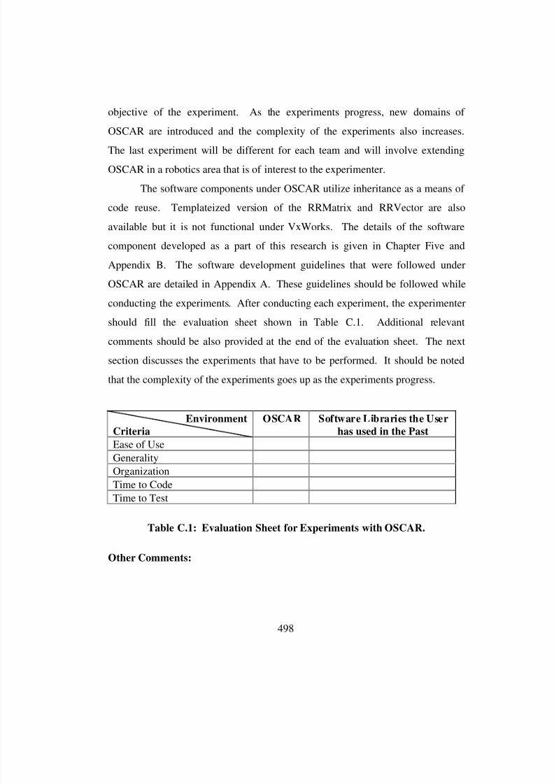
8/3/2019 Chetan Kapoor Dissertation
http://slidepdf.com/reader/full/chetan-kapoor-dissertation 519/612
498
objective of the experiment. As the experiments progress, new domains of
OSCAR are introduced and the complexity of the experiments also increases.
The last experiment will be different for each team and will involve extending
OSCAR in a robotics area that is of interest to the experimenter.
The software components under OSCAR utilize inheritance as a means of
code reuse. Templateized version of the RRMatrix and RRVector are also
available but it is not functional under VxWorks. The details of the software
component developed as a part of this research is given in Chapter Five and
Appendix B. The software development guidelines that were followed under
OSCAR are detailed in Appendix A. These guidelines should be followed while
conducting the experiments. After conducting each experiment, the experimenter
should fill the evaluation sheet shown in Table C.1. Additional relevant
comments should be also provided at the end of the evaluation sheet. The next
section discusses the experiments that have to be performed. It should be noted
that the complexity of the experiments goes up as the experiments progress.
Environment
Criteria
OSCAR Software Libraries the User
has used in the Past
Ease of Use
Generality
Organization
Time to Code
Time to Test
Table C.1: Evaluation Sheet for Experiments with OSCAR.
Other Comments:
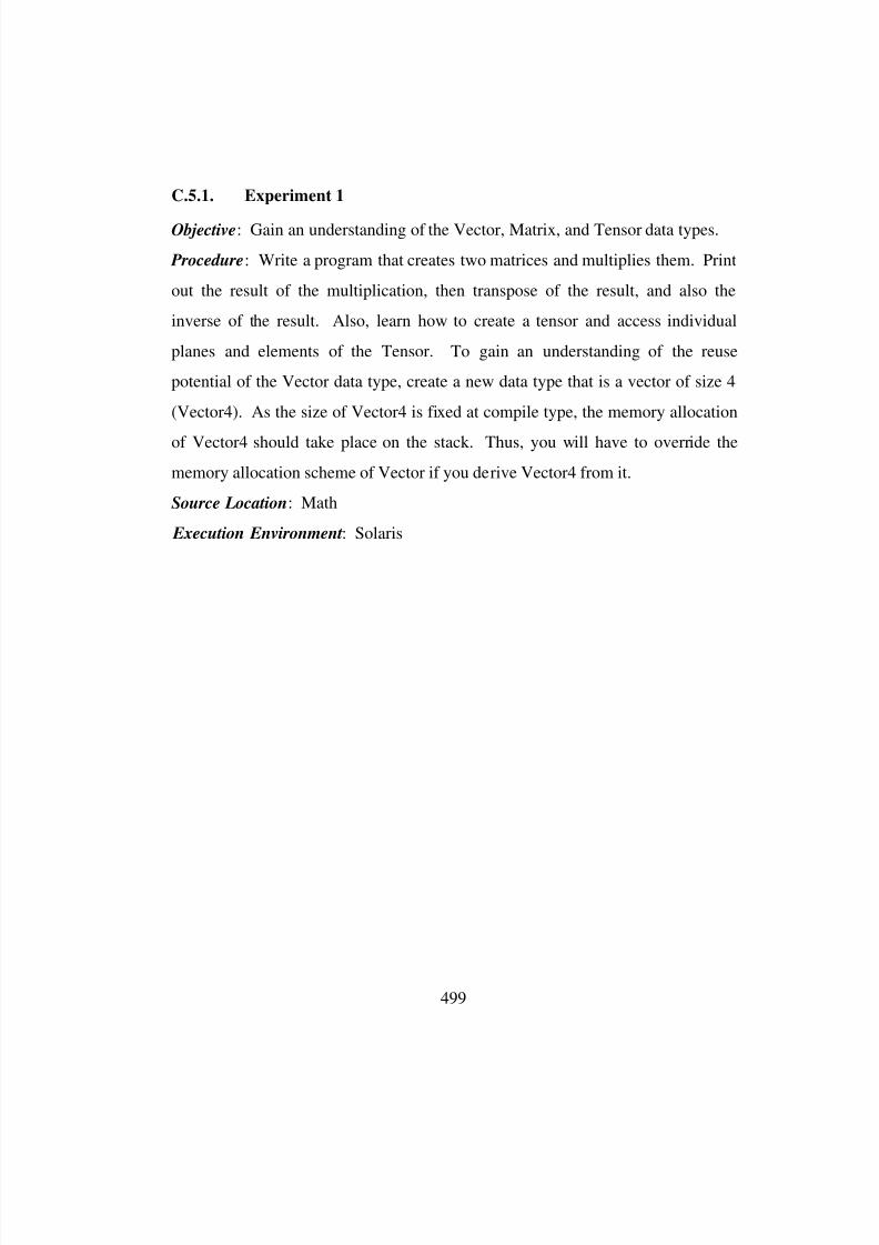
8/3/2019 Chetan Kapoor Dissertation
http://slidepdf.com/reader/full/chetan-kapoor-dissertation 520/612
499
C.5.1. Experiment 1
Objective: Gain an understanding of the Vector, Matrix, and Tensor data types.
Procedure: Write a program that creates two matrices and multiplies them. Print
out the result of the multiplication, then transpose of the result, and also the
inverse of the result. Also, learn how to create a tensor and access individual
planes and elements of the Tensor. To gain an understanding of the reuse
potential of the Vector data type, create a new data type that is a vector of size 4
(Vector4). As the size of Vector4 is fixed at compile type, the memory allocation
of Vector4 should take place on the stack. Thus, you will have to override the
memory allocation scheme of Vector if you derive Vector4 from it.
Source Location: Math
Execution Environment: Solaris
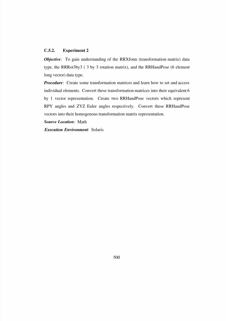
8/3/2019 Chetan Kapoor Dissertation
http://slidepdf.com/reader/full/chetan-kapoor-dissertation 521/612
500
C.5.2. Experiment 2
Objective: To gain understanding of the RRXform (transformation matrix) data
type, the RRRot3by3 ( 3 by 3 rotation matrix), and the RRHandPose (6 element
long vector) data type.
Procedure: Create some transformation matrices and learn how to set and access
individual elements. Convert these transformation matrices into their equivalent 6
by 1 vector representation. Create two RRHandPose vectors which represent
RPY angles and ZYZ Euler angles respectively. Convert these RRHandPose
vectors into their homogenous transformation matrix representation.
Source Location: Math
Execution Environment: Solaris
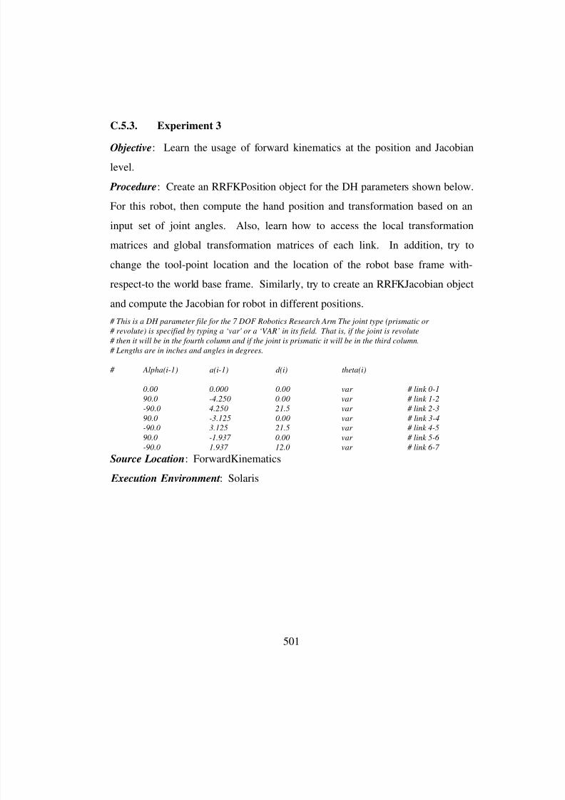
8/3/2019 Chetan Kapoor Dissertation
http://slidepdf.com/reader/full/chetan-kapoor-dissertation 522/612
501
C.5.3. Experiment 3
Objective: Learn the usage of forward kinematics at the position and Jacobian
level.
Procedure: Create an RRFKPosition object for the DH parameters shown below.
For this robot, then compute the hand position and transformation based on an
input set of joint angles. Also, learn how to access the local transformation
matrices and global transformation matrices of each link. In addition, try to
change the tool-point location and the location of the robot base frame with-
respect-to the world base frame. Similarly, try to create an RRFKJacobian object
and compute the Jacobian for robot in different positions.
# This is a DH parameter file for the 7 DOF Robotics Research Arm The joint type (prismatic or
# revolute) is specified by typing a ‘var' or a ‘VAR’ in its field. That is, if the joint is revolute
# then it will be in the fourth column and if the joint is prismatic it will be in the third column.
# Lengths are in inches and angles in degrees.
# Alpha(i-1) a(i-1) d(i) theta(i)
0.00 0.000 0.00 var # link 0-1
90.0 -4.250 0.00 var # link 1-2
-90.0 4.250 21.5 var # link 2-3
90.0 -3.125 0.00 var # link 3-4-90.0 3.125 21.5 var # link 4-5
90.0 -1.937 0.00 var # link 5-6
-90.0 1.937 12.0 var # link 6-7
Source Location: ForwardKinematics
Execution Environment: Solaris

8/3/2019 Chetan Kapoor Dissertation
http://slidepdf.com/reader/full/chetan-kapoor-dissertation 523/612
502
C.5.4. Experiment 4
Objective: Learn the usage of forward kinematics at the velocity and acceleration-
level.
Procedure: Create RRFKVelocity and RRFKAcceleration objects for the robot
whose DH parameters are described in experiment 2. Using these objects, learn
how to compute the rotational and translational G and H functions.
Source Location: ForwardKinematics
Execution Environment: Solaris
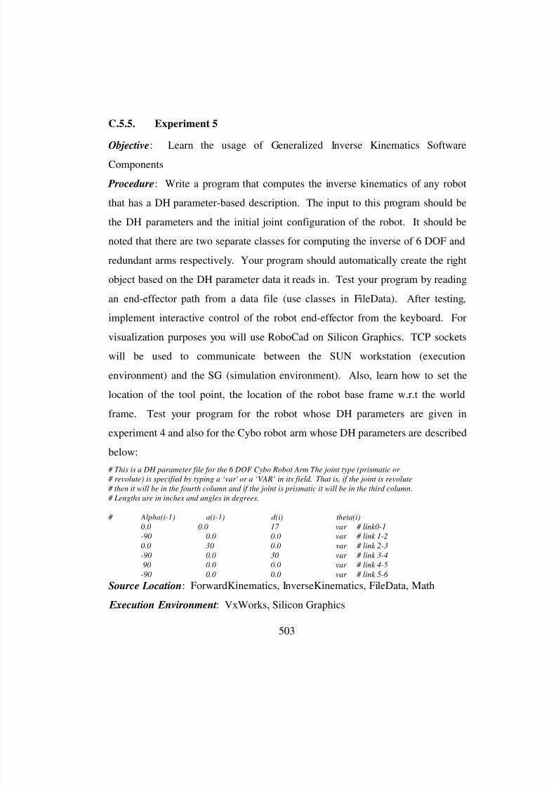
8/3/2019 Chetan Kapoor Dissertation
http://slidepdf.com/reader/full/chetan-kapoor-dissertation 524/612
503
C.5.5. Experiment 5
Objective: Learn the usage of Generalized Inverse Kinematics Software
Components
Procedure: Write a program that computes the inverse kinematics of any robot
that has a DH parameter-based description. The input to this program should be
the DH parameters and the initial joint configuration of the robot. It should be
noted that there are two separate classes for computing the inverse of 6 DOF and
redundant arms respectively. Your program should automatically create the right
object based on the DH parameter data it reads in. Test your program by reading
an end-effector path from a data file (use classes in FileData). After testing,
implement interactive control of the robot end-effector from the keyboard. For
visualization purposes you will use RoboCad on Silicon Graphics. TCP sockets
will be used to communicate between the SUN workstation (execution
environment) and the SG (simulation environment). Also, learn how to set the
location of the tool point, the location of the robot base frame w.r.t the world
frame. Test your program for the robot whose DH parameters are given in
experiment 4 and also for the Cybo robot arm whose DH parameters are described
below:
# This is a DH parameter file for the 6 DOF Cybo Robot Arm The joint type (prismatic or
# revolute) is specified by typing a ‘var' or a ‘VAR’ in its field. That is, if the joint is revolute
# then it will be in the fourth column and if the joint is prismatic it will be in the third column.
# Lengths are in inches and angles in degrees.
# Alpha(i-1) a(i-1) d(i) theta(i)
0.0 0.0 17 var # link0-1
-90 0.0 0.0 var # link 1-2
0.0 30 0.0 var # link 2-3
-90 0.0 30 var # link 3-4
90 0.0 0.0 var # link 4-5
-90 0.0 0.0 var # link 5-6
Source Location: ForwardKinematics, InverseKinematics, FileData, Math
Execution Environment: VxWorks, Silicon Graphics
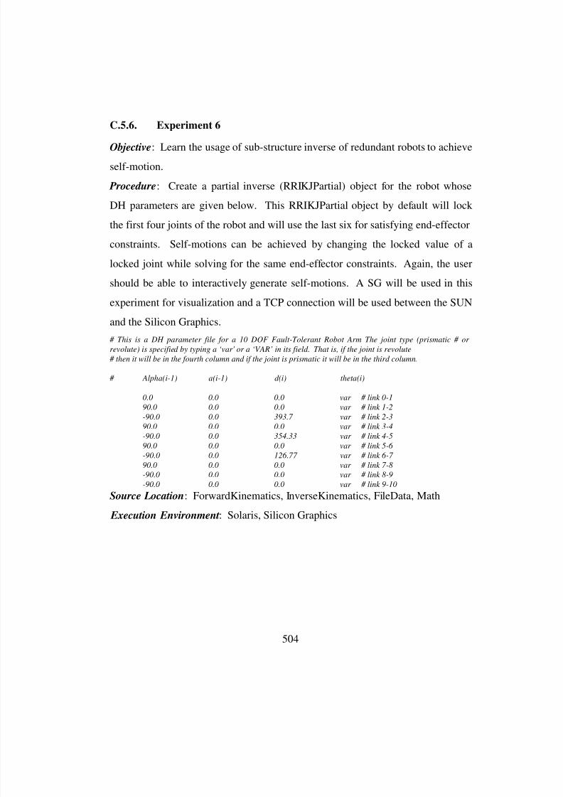
8/3/2019 Chetan Kapoor Dissertation
http://slidepdf.com/reader/full/chetan-kapoor-dissertation 525/612
504
C.5.6. Experiment 6
Objective: Learn the usage of sub-structure inverse of redundant robots to achieve
self-motion.
Procedure: Create a partial inverse (RRIKJPartial) object for the robot whose
DH parameters are given below. This RRIKJPartial object by default will lock
the first four joints of the robot and will use the last six for satisfying end-effector
constraints. Self-motions can be achieved by changing the locked value of a
locked joint while solving for the same end-effector constraints. Again, the user
should be able to interactively generate self-motions. A SG will be used in this
experiment for visualization and a TCP connection will be used between the SUN
and the Silicon Graphics.
# This is a DH parameter file for a 10 DOF Fault-Tolerant Robot Arm The joint type (prismatic # or
revolute) is specified by typing a ‘var' or a ‘VAR’ in its field. That is, if the joint is revolute
# then it will be in the fourth column and if the joint is prismatic it will be in the third column.
# Alpha(i-1) a(i-1) d(i) theta(i)
0.0 0.0 0.0 var # link 0-1
90.0 0.0 0.0 var # link 1-2
-90.0 0.0 393.7 var # link 2-390.0 0.0 0.0 var # link 3-4
-90.0 0.0 354.33 var # link 4-5
90.0 0.0 0.0 var # link 5-6
-90.0 0.0 126.77 var # link 6-7
90.0 0.0 0.0 var # link 7-8
-90.0 0.0 0.0 var # link 8-9
-90.0 0.0 0.0 var # link 9-10
Source Location: ForwardKinematics, InverseKinematics, FileData, Math
Execution Environment: Solaris, Silicon Graphics
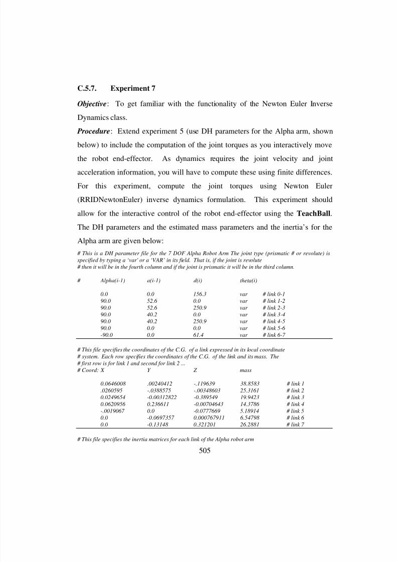
8/3/2019 Chetan Kapoor Dissertation
http://slidepdf.com/reader/full/chetan-kapoor-dissertation 526/612
505
C.5.7. Experiment 7
Objective: To get familiar with the functionality of the Newton Euler Inverse
Dynamics class.
Procedure: Extend experiment 5 (use DH parameters for the Alpha arm, shown
below) to include the computation of the joint torques as you interactively move
the robot end-effector. As dynamics requires the joint velocity and joint
acceleration information, you will have to compute these using finite differences.
For this experiment, compute the joint torques using Newton Euler
(RRIDNewtonEuler) inverse dynamics formulation. This experiment should
allow for the interactive control of the robot end-effector using the TeachBall.
The DH parameters and the estimated mass parameters and the inertia’s for the
Alpha arm are given below:
# This is a DH parameter file for the 7 DOF Alpha Robot Arm The joint type (prismatic # or revolute) is
specified by typing a ‘var' or a ‘VAR’ in its field. That is, if the joint is revolute
# then it will be in the fourth column and if the joint is prismatic it will be in the third column.
# Alpha(i-1) a(i-1) d(i) theta(i)
0.0 0.0 156.3 var # link 0-190.0 52.6 0.0 var # link 1-2
90.0 52.6 250.9 var # link 2-3
90.0 40.2 0.0 var # link 3-4
90.0 40.2 250.9 var # link 4-5
90.0 0.0 0.0 var # link 5-6
-90.0 0.0 61.4 var # link 6-7
# This file specifies the coordinates of the C.G. of a link expressed in its local coordinate
# system. Each row specifies the coordinates of the C.G. of the link and its mass. The
# first row is for link 1 and second for link 2 ...
# Coord: X Y Z mass
0.0646008 .00240412 -.119639 38.8583 # link 1
.0260595 -.0388575 -.00348603 25.3161 # link 2
0.0249654 -0.00312822 -0.389549 19.9423 # link 3
0.0620956 0.236611 -0.00704643 14.3786 # link 4
-.0019067 0.0 -0.0777669 5.18914 # link 5
0.0 -0.0697357 0.000767911 6.54798 # link 6
0.0 -0.13148 0.321201 26.2881 # link 7
# This file specifies the inertia matrices for each link of the Alpha robot arm

8/3/2019 Chetan Kapoor Dissertation
http://slidepdf.com/reader/full/chetan-kapoor-dissertation 527/612
506
.995849 0.0 0.0 # Inertia Tensor link 1
0.0 0.941168 0.0
0.0 0.0 0.25393
.40201 0.0 0.0 # Inertia Tensor Link 2
0.0 0.383098 0.0
0.0 0.0 0.17758
1.72994 0.0 0.0 # Inertia Tensor Link 3
0.0 1.70551 0.0
0.0 0.0 0.145429
0.85566 0.0 0.0 # Inertia Tensor Link 4
0.0 0.83904 0.0
0.0 0.0 0.0777043
0.0494478 0. 0.0 # Inertia Tensor Link 50.0 0.0477985 0.0
0.9 0.0 0.0137701
0.0518399 0.0 0.0 # Inertia Tensor Link 6
0.0 0.0508883 0.0
0.0 0.0 0.0169756
1.1081 0.0 0.0 # Inertia Tensor Link 7
0.0 1.10803 0.0
0.0 0.0 0.66374
Source Location: ForwardKinematics, InverseKinematics, InverseDynamics,
Math
Execution Environment: VxWorks, Silicon Graphics
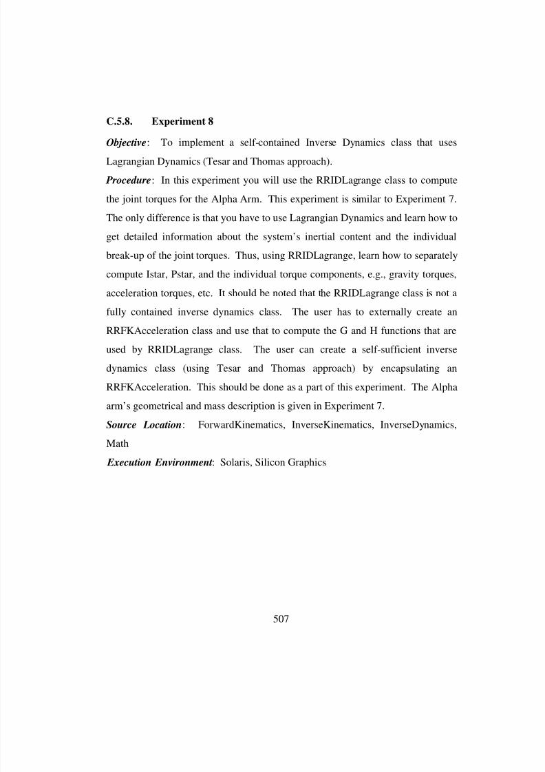
8/3/2019 Chetan Kapoor Dissertation
http://slidepdf.com/reader/full/chetan-kapoor-dissertation 528/612
507
C.5.8. Experiment 8
Objective: To implement a self-contained Inverse Dynamics class that uses
Lagrangian Dynamics (Tesar and Thomas approach).
Procedure: In this experiment you will use the RRIDLagrange class to compute
the joint torques for the Alpha Arm. This experiment is similar to Experiment 7.
The only difference is that you have to use Lagrangian Dynamics and learn how to
get detailed information about the system’s inertial content and the individual
break-up of the joint torques. Thus, using RRIDLagrange, learn how to separately
compute Istar, Pstar, and the individual torque components, e.g., gravity torques,
acceleration torques, etc. It should be noted that the RRIDLagrange class is not a
fully contained inverse dynamics class. The user has to externally create an
RRFKAcceleration class and use that to compute the G and H functions that are
used by RRIDLagrange class. The user can create a self-sufficient inverse
dynamics class (using Tesar and Thomas approach) by encapsulating an
RRFKAcceleration. This should be done as a part of this experiment. The Alpha
arm’s geometrical and mass description is given in Experiment 7.
Source Location: ForwardKinematics, InverseKinematics, InverseDynamics,
Math
Execution Environment: Solaris, Silicon Graphics

8/3/2019 Chetan Kapoor Dissertation
http://slidepdf.com/reader/full/chetan-kapoor-dissertation 529/612
508
C.5.9. Experiment 9
Objective: To learn the usage of the generalized deflection modeling software
components.
Procedure: Extend experiment 8 to include deflection modeling for the Alpha
arm. To every joint position that is output from the inverse kinematics object,
apply the generalized deflection model and compute the deflection at the end-
effector. Compensate for this end-effector deflection by adding the deflection to
the desired end-effector position. Based on this new end-effector position,
compute the inverse position solution and then compute the joint torques using
Newton-Euler. This experiment should also allow for interactive execution using
the SG for visualization. The estimated composite compliance (joint and link)
matrices for each link of the Alpha arm are given below:
# This file specifies the compliance matrices for the Alpha manipulator. Each matrix
# is 6x6.
# Joint-Link 1 compliance matrix4.76797e-09 -1.29363e-11 1.79584e-11 4.77269e-10 -2.65275e-09 -1.16114e-09
-1.29363e-11 3.66306e-09 1.23339e-09 -4.63556e-09 5.83829e-11 -1.7344e-10
1.79584e-11 1.23339e-09 1.22997e-09 -1.78723e-09 1.71979e-10 -9.23178e-11
4.77269e-10 -4.63556e-09 -1.78723e-09 0.0 0.0 0.0
-2.65275e-09 5.83829e-11 1.71979e-10 0.0 0.0 0.0
-1.16114e-09 -1.7344e-10 -9.23178e-11 0.0 0.0 0.0
# Joint-Link 2 compliance matrix
2.32974e-09 0.0 0.0 0.0 0.0 0.0
0.0 6.39137e-08 0.0 0.0 0.0 1.74227e-07
0.0 0.0 6.39137e-08 0.0 -1.74227e-07 0.0
0.0 0.0 0.0 8.23119e-07 0.0 0.0
0.0 0.0 -1.74227e-07 0.0 6.37254e-07 0.0
0.0 1.74227e-07 0.0 0.0 0.0 6.37254e-07
# Joint-Link 3 compliance matrix
7.09771e-09 -1.29363e-11 1.79584e-11 4.77269e-10 -2.65275e-09 -1.16114e-09
-1.29363e-11 6.75768e-08 1.23339e-09 -4.63556e-09 5.83829e-11 1.74054e-07 1.79584e-11 1.23339e-09 6.51437e-08 -1.78723e-09 -1.74055e-07 -9.23178e-11
4.77269e-10 -4.63556e-09 -1.78723e-09 8.23119e-07 0.0 0.0
-2.65275e-09 5.83829e-11 -1.74055e-07 0.0 6.37254e-07 0.0
-1.16114e-09 1.74054e-07 -9.23178e-11 0.0 0.0 6.37254e-07
# Joint-Link 4 compliance matrix
2.73687e-08 -8.49384e-09 -4.0542e-10 -2.19863e-09 -5.01211e-10 6.76225e-08
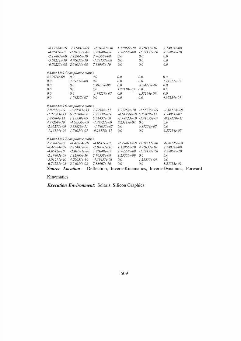
8/3/2019 Chetan Kapoor Dissertation
http://slidepdf.com/reader/full/chetan-kapoor-dissertation 530/612
509
-8.49384e-09 7.15481e-09 -2.04081e-10 1.12966e-10 4.76033e-10 2.54034e-08
-4.0542e-10 -2.04081e-10 1.70048e-08 2.70558e-08 -1.39157e-08 7.88967e-10
-2.19863e-09 1.12966e-10 2.70558e-08 0.0 0.0 0.0
-5.01211e-10 4.76033e-10 -1.39157e-08 0.0 0.0 0.0-6.76225e-08 2.54034e-08 7.88967e-10 0.0 0.0 0.0
# Joint-Link 5 compliance matrix
4.32974e-09 0.0 0.0 0.0 0.0 0.0
0.0 3.39137e-08 0.0 0.0 0.0 1.74227e-07
0.0 0.0 5.39137e-08 0.0 -1.74227e-07 0.0
0.0 0.0 0.0 3.23119e-07 0.0 0.0
0.0 0.0 -1.74227e-07 0.0 4.37254e-07 0.0
0.0 1.74227e-07 0.0 0.0 0.0 4.37254e-07
# Joint-Link 6 compliance matrix
7.09771e-09 -1.29363e-11 1.79584e-11 4.77269e-10 -2.65275e-09 -1.16114e-09
-1.29363e-11 6.75768e-08 1.23339e-09 -4.63556e-09 5.83829e-11 1.74054e-07
1.79584e-11 1.23339e-09 6.51437e-08 -1.78723e-09 -1.74055e-07 -9.23178e-114.77269e-10 -4.63556e-09 -1.78723e-09 8.23119e-07 0.0 0.0
-2.65275e-09 5.83829e-11 -1.74055e-07 0.0 6.37254e-07 0.0
-1.16114e-09 1.74054e-07 -9.23178e-11 0.0 0.0 6.37254e-07
# Joint-Link 7 compliance matrix
2.73687e-07 -8.49384e-09 -4.0542e-10 -2.19863e-09 -5.01211e-10 -6.76225e-08
-8.49384e-09 7.15481e-08 -2.04081e-10 1.12966e-10 4.76033e-10 2.54034e-08
-4.0542e-10 -2.04081e-10 1.70048e-07 2.70558e-08 -1.39157e-08 7.88967e-10
-2.19863e-09 1.12966e-10 2.70558e-08 1.25555e-09 0.0 0.0
-5.01211e-10 4.76033e-10 -1.39157e-08 0.0 1.25555e-09 0.0
-6.76225e-08 2.54034e-08 7.88967e-10 0.0 0.0 1.25555e-09
Source Location: Deflection, InverseKinematics, InverseDynamics, Forward
Kinematics Execution Environment: Solaris, Silicon Graphics

8/3/2019 Chetan Kapoor Dissertation
http://slidepdf.com/reader/full/chetan-kapoor-dissertation 531/612
510
C.5.10. Experiment 10
Objective: To design and implement software components in your area of interest
and expertise.
Procedure: To be discussed with Dr. Hooper and Dr. Tesar.
8/3/2019 Chetan Kapoor Dissertation
http://slidepdf.com/reader/full/chetan-kapoor-dissertation 532/612
511
C.6. User Qualification Assessment
User qualification assessment was necessary for normalizing the results of
the experiments based on user experience, aptitude, and motivation. A measure
of the experimenter qualification and aptitude was achieved by consultation with
the experimenter’s academic supervisor and by monitoring their progress over the
course of the experiments. To gauge user qualification, a survey was performed
that measured four things. These were:
Experience with object-oriented programming using C++.
An understanding of the domain of advanced robotics.
Experience with the software system the experimenter is comparing to
OSCAR.
How closely does the compared software system satisfy operational software
needs of advanced robotics (that is, the main purpose of OSCAR).
The survey used for measuring the user qualifications is shown below:
On a scale of 1 to 10, how would you gauge your experience with the software
system you are comparing OSCAR with, to programming in a C, C++ type
environment (use experience level prior to the beginning of the experiments)?
C/C++ Type _________ Compared Software System ____________
How many Robotics related undergraduate courses have you had? _________
How many Robotics related graduate courses have you had? ______________
How many Linear Algebra math courses have you had? ______________
What is the primary software system you were comparing OSCAR too (give
details)? _______________________________________________________
_________________________________________________________________
_________________________________________________________________
_________________________________________________________________
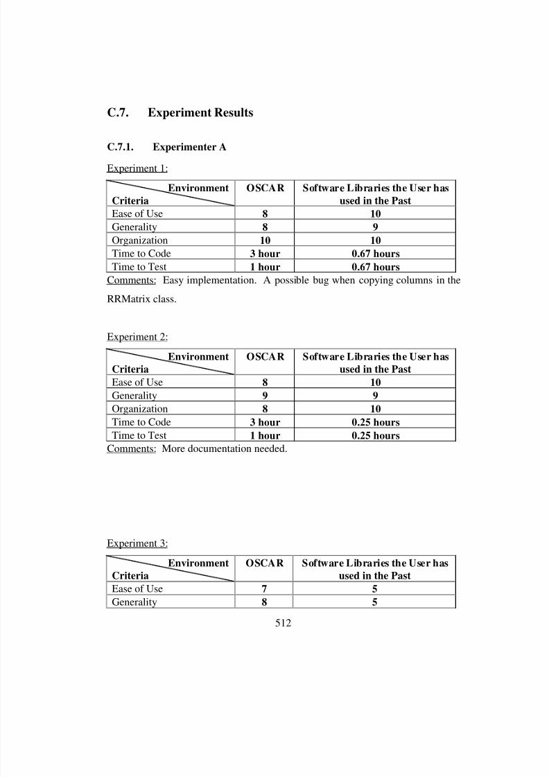
8/3/2019 Chetan Kapoor Dissertation
http://slidepdf.com/reader/full/chetan-kapoor-dissertation 533/612
512
C.7. Experiment Results
C.7.1. Experimenter A
Experiment 1:
Environment
Criteria
OSCAR Software Libraries the User has
used in the Past
Ease of Use 8 10
Generality 8 9
Organization 10 10
Time to Code 3 hour 0.67 hours
Time to Test 1 hour 0.67 hoursComments: Easy implementation. A possible bug when copying columns in the
RRMatrix class.
Experiment 2:
Environment
Criteria
OSCAR Software Libraries the User has
used in the Past
Ease of Use 8 10
Generality 9 9
Organization 8 10Time to Code 3 hour 0.25 hours
Time to Test 1 hour 0.25 hours
Comments: More documentation needed.
Experiment 3:
Environment
Criteria
OSCAR Software Libraries the User has
used in the Past
Ease of Use 7 5
Generality 8 5

8/3/2019 Chetan Kapoor Dissertation
http://slidepdf.com/reader/full/chetan-kapoor-dissertation 534/612
513
Organization 10 5
Time to Code 5 hour 10 hours
Time to Test 1 hour 1 hourComments:
Experiment 4:
Environment
Criteria
OSCAR Software Libraries the User has
used in the Past
Ease of Use 8 5
Generality 9 5
Organization 10 5
Time to Code 2 hour 10 hours
Time to Test 1 hour 1 hourComments:
Experiment 5:
Environment
Criteria
OSCAR Software Libraries the User has
used in the Past
Ease of Use 7 7
Generality 10 4
Organization 10 5
Time to Code 10 hours 10 hoursTime to Test 1 hour 1 hour
Comments:
Experiment 6:
Environment
Criteria
OSCAR Software Libraries the User has
used in the Past
Ease of Use 9 5
Generality 8 5
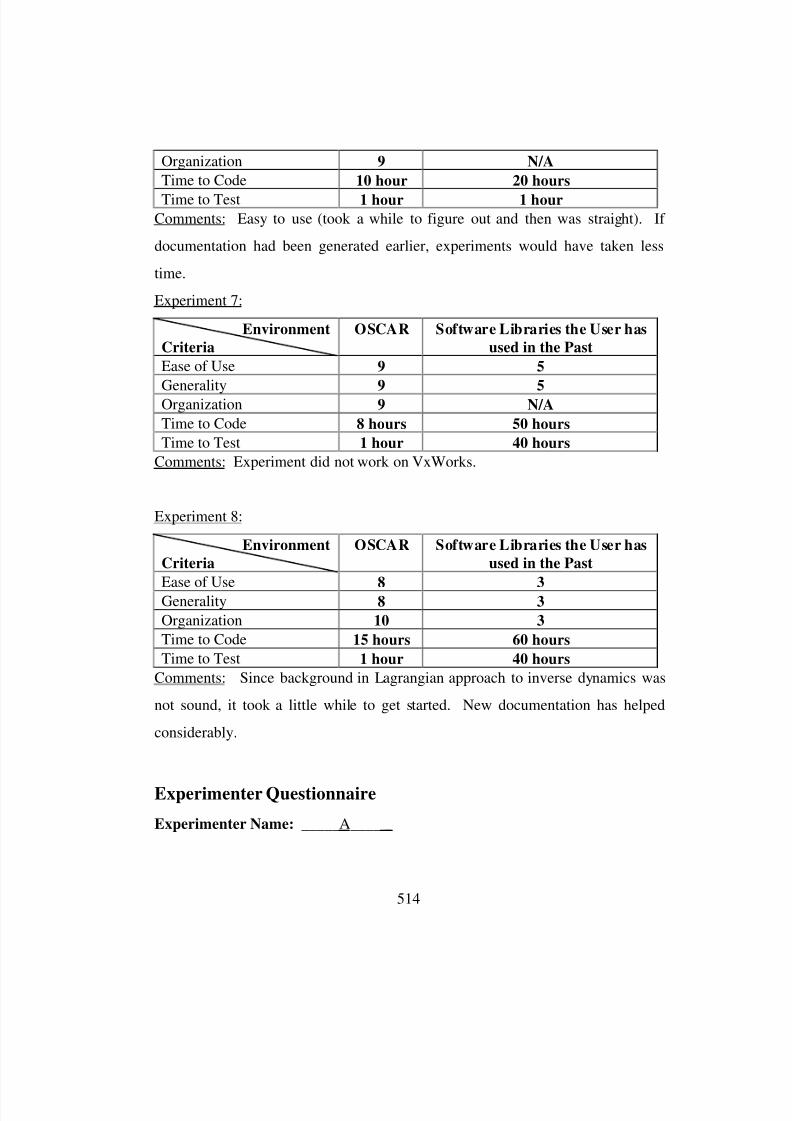
8/3/2019 Chetan Kapoor Dissertation
http://slidepdf.com/reader/full/chetan-kapoor-dissertation 535/612
514
Organization 9 N/A
Time to Code 10 hour 20 hours
Time to Test 1 hour 1 hourComments: Easy to use (took a while to figure out and then was straight). If
documentation had been generated earlier, experiments would have taken less
time.
Experiment 7:
Environment
Criteria
OSCAR Software Libraries the User has
used in the Past
Ease of Use 9 5
Generality 9 5Organization 9 N/A
Time to Code 8 hours 50 hours
Time to Test 1 hour 40 hours
Comments: Experiment did not work on VxWorks.
Experiment 8:
Environment
Criteria
OSCAR Software Libraries the User has
used in the Past
Ease of Use 8 3Generality 8 3
Organization 10 3
Time to Code 15 hours 60 hours
Time to Test 1 hour 40 hours
Comments: Since background in Lagrangian approach to inverse dynamics was
not sound, it took a little while to get started. New documentation has helped
considerably.
Experimenter Questionnaire
Experimenter Name: _____A____ _

8/3/2019 Chetan Kapoor Dissertation
http://slidepdf.com/reader/full/chetan-kapoor-dissertation 536/612
515
On a scale of 1 to 10, how would you gauge your experience with the software
system you are comparing OSCAR with, to programming in C/C++ type
environment (use experience level prior to the beginning of the experiments)?
C/C++ Type ____7____ Compared Software System _____5_____
How many Robotics related undergraduate courses have you had? __ 0____
How many Robotics related graduate courses have you had? _____1_______
How many Linear Algebra math courses have you had? ______2_______
What is the primary software system you were comparing OSCAR too (give
details)?
Mainly my experience in software systems for robotics applications is related
to Matlab. Basically I developed small "objects" to calculate Inverse/Forward
kinematics and used "spatial notation" taught by Dr. Sreenivasan. One of the
most noticeable limitations of Matlab was its lack of support for 3-
Dimensional matrices/Tensor like objects. Although, different files
corresponded to different, independent objects, they were not quite modular,
that is, corrections/modifications in an object had to be propagated
"propagated" manually in other files.
Averaged Evaluation Data
Environment
Criteria
OSCAR Software Libraries the User has
used in the Past
Ease of Use 8 6.25
Generality 8.50 5.63
Organization 9.67 6.33
Time to Code 3.47 10
Time to Test 0.37 0.31
C.7.2. Experimenter B
Experiment 1:
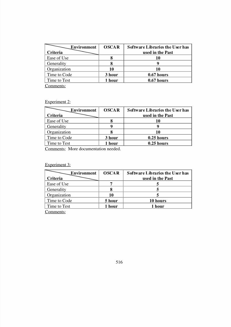
8/3/2019 Chetan Kapoor Dissertation
http://slidepdf.com/reader/full/chetan-kapoor-dissertation 537/612
516
Environment
Criteria
OSCAR Software Libraries the User has
used in the Past
Ease of Use 8 10Generality 8 9
Organization 10 10
Time to Code 3 hour 0.67 hours
Time to Test 1 hour 0.67 hours
Comments:
Experiment 2:
Environment
Criteria
OSCAR Software Libraries the User has
used in the PastEase of Use 8 10
Generality 9 9
Organization 8 10
Time to Code 3 hour 0.25 hours
Time to Test 1 hour 0.25 hours
Comments: More documentation needed.
Experiment 3:
EnvironmentCriteria
OSCAR Software Libraries the User hasused in the Past
Ease of Use 7 5
Generality 8 5
Organization 10 5
Time to Code 5 hour 10 hours
Time to Test 1 hour 1 hour
Comments:
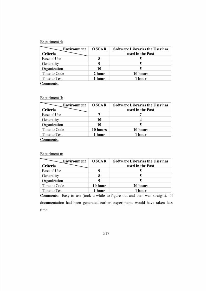
8/3/2019 Chetan Kapoor Dissertation
http://slidepdf.com/reader/full/chetan-kapoor-dissertation 538/612
517
Experiment 4:
EnvironmentCriteria OSCAR Software Libraries the User hasused in the Past
Ease of Use 8 5
Generality 9 5
Organization 10 5
Time to Code 2 hour 10 hours
Time to Test 1 hour 1 hour
Comments:
Experiment 5:
Environment
Criteria
OSCAR Software Libraries the User has
used in the Past
Ease of Use 7 7
Generality 10 4
Organization 10 5
Time to Code 10 hours 10 hours
Time to Test 1 hour 1 hour
Comments:
Experiment 6:
Environment
Criteria
OSCAR Software Libraries the User has
used in the Past
Ease of Use 9 5
Generality 8 5
Organization 9 5
Time to Code 10 hour 20 hours
Time to Test 1 hour 1 hour
Comments: Easy to use (took a while to figure out and then was straight). If
documentation had been generated earlier, experiments would have taken lesstime.

8/3/2019 Chetan Kapoor Dissertation
http://slidepdf.com/reader/full/chetan-kapoor-dissertation 539/612
518
Experiment 7:
EnvironmentCriteria OSCAR Software Libraries the User hasused in the Past
Ease of Use 9 5
Generality 9 5
Organization 9 N/A
Time to Code 8 hours 50 hours
Time to Test 1 hour 40 hours
Comments: Experiment did not work on VxWorks.
Experiment 8:
Environment
Criteria
OSCAR Software Libraries the User has
used in the Past
Ease of Use 8 3
Generality 8 3
Organization 10 3
Time to Code 15 hours 60 hours
Time to Test 1 hour 40 hours
Comments:
Experiment 10:
Environment
Criteria
OSCAR Software Libraries the User has
used in the Past
Ease of Use 9 5
Generality 9 2
Organization 10 4
Time to Code 60 hours 300 hours
Time to Test 180 hours 500 hours
Comments: In general all classes have rapid-prototyping capability and for this
reason they are quite extensible. Adding short examples on how to use a class (inthe appendix) would give a stronger reference to the programmer, especially if
he/she is novice in the field.
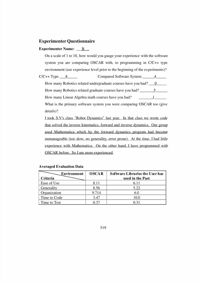
8/3/2019 Chetan Kapoor Dissertation
http://slidepdf.com/reader/full/chetan-kapoor-dissertation 540/612
519
Experimenter Questionnaire
Experimenter Name: ___B _ On a scale of 1 to 10, how would you gauge your experience with the software
system you are comparing OSCAR with, to programming in C/C++ type
environment (use experience level prior to the beginning of the experiments)?
C/C++ Type ___8_____ Compared Software System ______4_____
How many Robotics related undergraduate courses have you had? ___0_____
How many Robotics related graduate courses have you had? _______5______
How many Linear Algebra math courses have you had? _______1______
What is the primary software system you were comparing OSCAR too (give
details)?
I took S.V’s class "Robot Dynamics" last year. In that class we wrote code
that solved the inverse kinematics, forward and inverse dynamics. Our group
used Mathematica which by the forward dynamics program had become
unmanageable (too slow, no generality, error prone). At the time, I had little
experience with Mathematica. On the other hand, I have programmed with
OSCAR before. So I am more experienced.
Averaged Evaluation Data
Environment
Criteria
OSCAR Software Libraries the User has
used in the Past
Ease of Use 8.11 6.11
Generality 8.56 5.22
Organization 9.714 6.0
Time to Code 3.47 10.0Time to Test 0.37 0.31
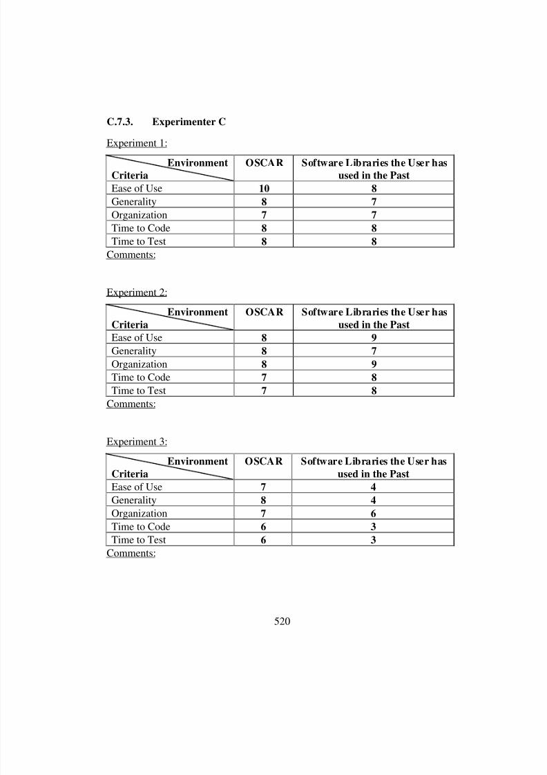
8/3/2019 Chetan Kapoor Dissertation
http://slidepdf.com/reader/full/chetan-kapoor-dissertation 541/612
520
C.7.3. Experimenter C
Experiment 1:
Environment
Criteria
OSCAR Software Libraries the User has
used in the Past
Ease of Use 10 8
Generality 8 7
Organization 7 7
Time to Code 8 8
Time to Test 8 8
Comments:
Experiment 2:
Environment
Criteria
OSCAR Software Libraries the User has
used in the Past
Ease of Use 8 9
Generality 8 7
Organization 8 9
Time to Code 7 8
Time to Test 7 8
Comments:
Experiment 3:
Environment
Criteria
OSCAR Software Libraries the User has
used in the Past
Ease of Use 7 4
Generality 8 4
Organization 7 6
Time to Code 6 3
Time to Test 6 3Comments:
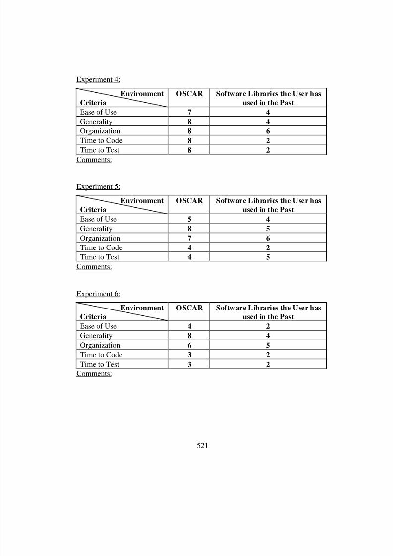
8/3/2019 Chetan Kapoor Dissertation
http://slidepdf.com/reader/full/chetan-kapoor-dissertation 542/612
521
Experiment 4:
EnvironmentCriteria OSCAR Software Libraries the User hasused in the Past
Ease of Use 7 4
Generality 8 4
Organization 8 6
Time to Code 8 2
Time to Test 8 2
Comments:
Experiment 5:
Environment
Criteria
OSCAR Software Libraries the User has
used in the Past
Ease of Use 5 4
Generality 8 5
Organization 7 6
Time to Code 4 2
Time to Test 4 5
Comments:
Experiment 6:
Environment
Criteria
OSCAR Software Libraries the User has
used in the Past
Ease of Use 4 2
Generality 8 4
Organization 6 5
Time to Code 3 2
Time to Test 3 2
Comments:
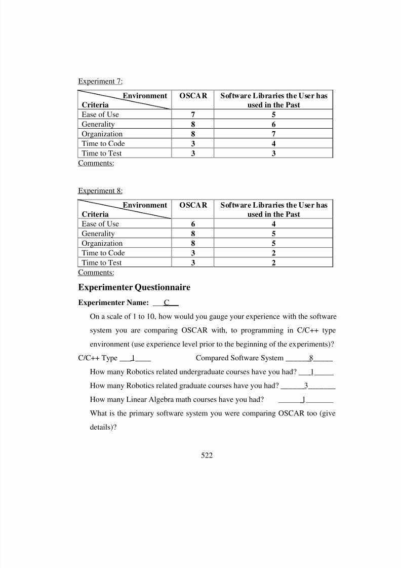
8/3/2019 Chetan Kapoor Dissertation
http://slidepdf.com/reader/full/chetan-kapoor-dissertation 543/612
522
Experiment 7:
EnvironmentCriteria OSCAR Software Libraries the User hasused in the Past
Ease of Use 7 5
Generality 8 6
Organization 8 7
Time to Code 3 4
Time to Test 3 3
Comments:
Experiment 8:
Environment
Criteria
OSCAR Software Libraries the User has
used in the Past
Ease of Use 6 4
Generality 8 5
Organization 8 5
Time to Code 3 2
Time to Test 3 2
Comments:
Experimenter Questionnaire
Experimenter Name: ___C _
On a scale of 1 to 10, how would you gauge your experience with the software
system you are comparing OSCAR with, to programming in C/C++ type
environment (use experience level prior to the beginning of the experiments)?
C/C++ Type ___1____ Compared Software System ______8_____
How many Robotics related undergraduate courses have you had? ___1_____
How many Robotics related graduate courses have you had? ______3_______
How many Linear Algebra math courses have you had? ______1_______
What is the primary software system you were comparing OSCAR too (give
details)?

8/3/2019 Chetan Kapoor Dissertation
http://slidepdf.com/reader/full/chetan-kapoor-dissertation 544/612
523
Matlab - a mathematical package that I have used to perform robot
simulations.
Averaged Evaluation Data
Environment
Criteria
OSCAR Software Libraries the User has
used in the Past
Ease of Use 6.75 5.0
Generality 8.0 5.25
Organization 7.375 6.25
Time to Code 4.25 5.875
Time to Test 4.25 5.25

8/3/2019 Chetan Kapoor Dissertation
http://slidepdf.com/reader/full/chetan-kapoor-dissertation 545/612
524
C.7.4. Experimenter D
Experiment 1:
Environment
Criteria
OSCAR Software Libraries the User has
used in the Past
Ease of Use 8 9
Generality 9 9
Organization 9 3
Time to Code 8 2
Time to Test 9 1
Comments: All comparisons of this and other five experiments are made among
OSCAR and the symbolic manipulation language, REDUCE, environment.
REDUCE is supposedly an interactive environment. Although time-consuming, it
is possible to write small program modules in REDUCE which can later be
combined to create a "structured" program.
Experiment 2:
Environment
Criteria
OSCAR Software Libraries the User has
used in the Past
Ease of Use 8 6
Generality 8 8Organization 9 2
Time to Code 9 1
Time to Test 10 0
Comments:
Experiment 3:
Environment
Criteria
OSCAR Software Libraries the User has
used in the Past
Ease of Use 7 5
Generality 8 6Organization 8 3
Time to Code 9 2
Time to Test 9 1
Comments:
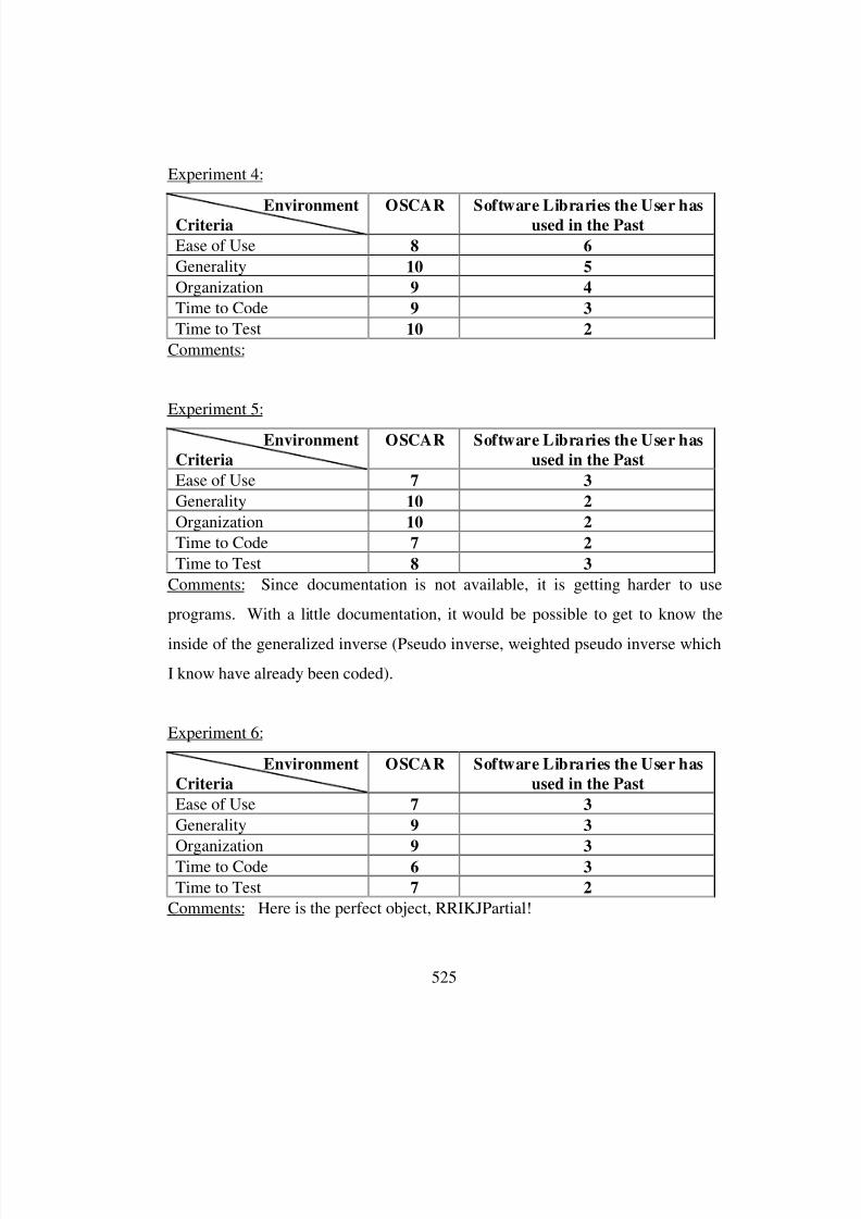
8/3/2019 Chetan Kapoor Dissertation
http://slidepdf.com/reader/full/chetan-kapoor-dissertation 546/612
525
Experiment 4:
EnvironmentCriteria OSCAR Software Libraries the User hasused in the Past
Ease of Use 8 6
Generality 10 5
Organization 9 4
Time to Code 9 3
Time to Test 10 2
Comments:
Experiment 5:
Environment
Criteria
OSCAR Software Libraries the User has
used in the Past
Ease of Use 7 3
Generality 10 2
Organization 10 2
Time to Code 7 2
Time to Test 8 3
Comments: Since documentation is not available, it is getting harder to use
programs. With a little documentation, it would be possible to get to know the
inside of the generalized inverse (Pseudo inverse, weighted pseudo inverse which
I know have already been coded).
Experiment 6:
Environment
Criteria
OSCAR Software Libraries the User has
used in the Past
Ease of Use 7 3
Generality 9 3
Organization 9 3Time to Code 6 3
Time to Test 7 2
Comments: Here is the perfect object, RRIKJPartial!

8/3/2019 Chetan Kapoor Dissertation
http://slidepdf.com/reader/full/chetan-kapoor-dissertation 547/612
526
Experimenter Questionnaire
Experimenter Name: ___D _ On a scale of 1 to 10, how would you gauge your experience with the software
system you are comparing OSCAR with, to programming in C/C++ type
environment (use experience level prior to the beginning of the experiments)?
C/C++ Type ___3____ Compared Software System ______4_____
How many Robotics related undergraduate courses have you had? ___2_____
How many Robotics related graduate courses have you had? _______4______
How many Linear Algebra math courses have you had? _______1______
What is the primary software system you were comparing OSCAR with (give
details)?
Symbolic manipulation language REDUCE. Had numerical built-in functions
too. Interactive environment but allows structured programming. Hard to
program though due to lack of debugging environment. REDUCE is more
comparable to MAPLE, less fancier than Mathematica (no graphic
environment). One advantage is however is that the built-in functions are
available for modification and a considerable amount of source code is
available for purposes.
Averaged Evaluation Data
Environment
Criteria
OSCAR Software Libraries the User has
used in the Past
Ease of Use 7.5 5.33
Generality 9.0 5.5
Organization 7.33 2.83Time to Code 2.16 8.0
Time to Test 1.5 8.33
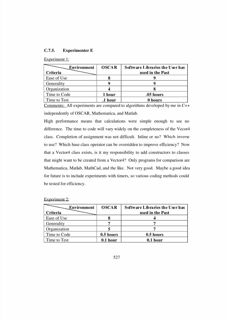
8/3/2019 Chetan Kapoor Dissertation
http://slidepdf.com/reader/full/chetan-kapoor-dissertation 548/612
527
C.7.5. Experimenter E
Experiment 1:
Environment
Criteria
OSCAR Software Libraries the User has
used in the Past
Ease of Use 8 9
Generality 9 9
Organization 4 8
Time to Code 1 hour .05 hours
Time to Test .1 hour 0 hours
Comments: All experiments are compared to algorithms developed by me in C++
independently of OSCAR, Mathematica, and Matlab.
High performance means that calculations were simple enough to see no
difference. The time to code will vary widely on the completeness of the Vecor4
class. Completion of assignment was not difficult. Inline or no? Which inverse
to use? Which base class operator can be overridden to improve efficiency? Now
that a Vector4 class exists, is it my responsibility to add constructors to classes
that might want to be created from a Vector4? Only programs for comparison are
Mathematica, Matlab, MathCad, and the like. Not very good. Maybe a good idea
for future is to include experiments with timers, so various coding methods could
be tested for efficiency.
Experiment 2:
Environment
Criteria
OSCAR Software Libraries the User has
used in the Past
Ease of Use 8 4
Generality 7 7Organization 5 7
Time to Code 0.5 hours 0.5 hours
Time to Test 0.1 hour 0.1 hour
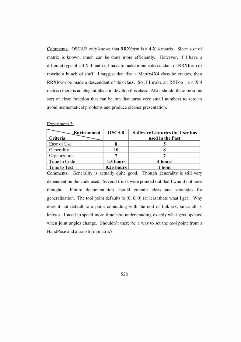
8/3/2019 Chetan Kapoor Dissertation
http://slidepdf.com/reader/full/chetan-kapoor-dissertation 549/612
528
Comments: OSCAR only knows that RRXform is a 4 X 4 matrix. Since size of
matrix is known, much can be done more efficiently. However, if I have a
different type of a 4 X 4 matrix, I have to make mine a descendant of RRXform or
rewrite a bunch of stuff. I suggest that first a Matrix4X4 class be creates, then
RRXform be made a descendant of this class. So if I make an RRFoo ( a 4 X 4
matrix) there is an elegant place to develop this class. Also, should there be some
sort of clean function that can be run that turns very small numbers to zero to
avoid mathematical problems and produce cleaner presentation.
Experiment 3:
Environment
Criteria
OSCAR Software Libraries the User has
used in the Past
Ease of Use 8 5
Generality 10 8
Organization 7 7
Time to Code 1.5 hours 4 hours
Time to Test 0.25 hours 1 hour
Comments: Generality is actually quite good. Though generality is still very
dependent on the code used. Several tricks were pointed out that I would not have
thought. Future documentation should contain ideas and strategies for
generalization. The tool point defaults to [0, 0, 0] (at least thats what I get). Why
does it not default to a point coinciding with the end of link six, since all is
known. I need to spend more time here understanding exactly what gets updated
when joint angles change. Shouldn’t there be a way to set the tool point from a
HandPose and a transform matrix?
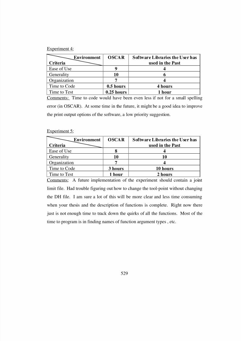
8/3/2019 Chetan Kapoor Dissertation
http://slidepdf.com/reader/full/chetan-kapoor-dissertation 550/612
529
Experiment 4:
EnvironmentCriteria OSCAR Software Libraries the User hasused in the Past
Ease of Use 9 4
Generality 10 6
Organization 7 4
Time to Code 0.5 hours 4 hours
Time to Test 0.25 hours 1 hour
Comments: Time to code would have been even less if not for a small spelling
error (in OSCAR). At some time in the future, it might be a good idea to improve
the print output options of the software, a low priority suggestion.
Experiment 5:
Environment
Criteria
OSCAR Software Libraries the User has
used in the Past
Ease of Use 8 4
Generality 10 10
Organization 7 4
Time to Code 3 hours 10 hours
Time to Test 1 hour 2 hours
Comments: A future implementation of the experiment should contain a joint
limit file. Had trouble figuring out how to change the tool-point without changing
the DH file. I am sure a lot of this will be more clear and less time consuming
when your thesis and the description of functions is complete. Right now there
just is not enough time to track down the quirks of all the functions. Most of the
time to program is in finding names of function argument types , etc.
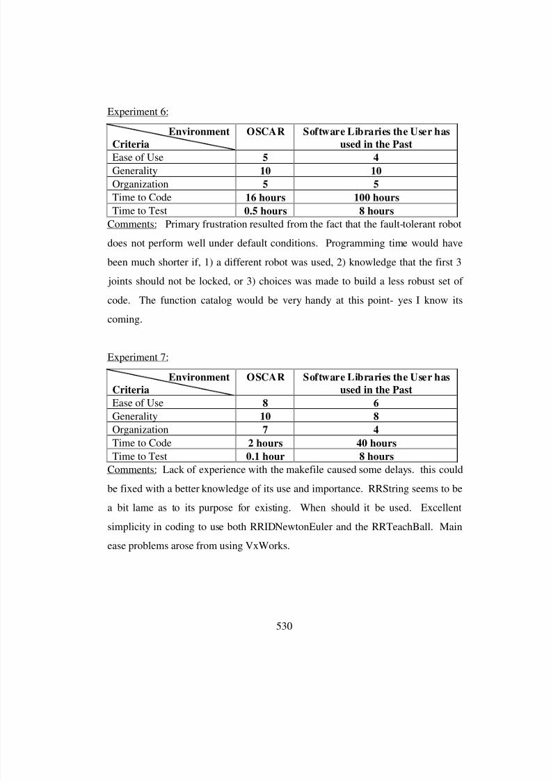
8/3/2019 Chetan Kapoor Dissertation
http://slidepdf.com/reader/full/chetan-kapoor-dissertation 551/612
530
Experiment 6:
EnvironmentCriteria OSCAR Software Libraries the User hasused in the Past
Ease of Use 5 4
Generality 10 10
Organization 5 5
Time to Code 16 hours 100 hours
Time to Test 0.5 hours 8 hours
Comments: Primary frustration resulted from the fact that the fault-tolerant robot
does not perform well under default conditions. Programming time would have
been much shorter if, 1) a different robot was used, 2) knowledge that the first 3
joints should not be locked, or 3) choices was made to build a less robust set of
code. The function catalog would be very handy at this point- yes I know its
coming.
Experiment 7:
Environment
Criteria
OSCAR Software Libraries the User has
used in the Past
Ease of Use 8 6
Generality 10 8
Organization 7 4
Time to Code 2 hours 40 hours
Time to Test 0.1 hour 8 hours
Comments: Lack of experience with the makefile caused some delays. this could
be fixed with a better knowledge of its use and importance. RRString seems to be
a bit lame as to its purpose for existing. When should it be used. Excellent
simplicity in coding to use both RRIDNewtonEuler and the RRTeachBall. Main
ease problems arose from using VxWorks.
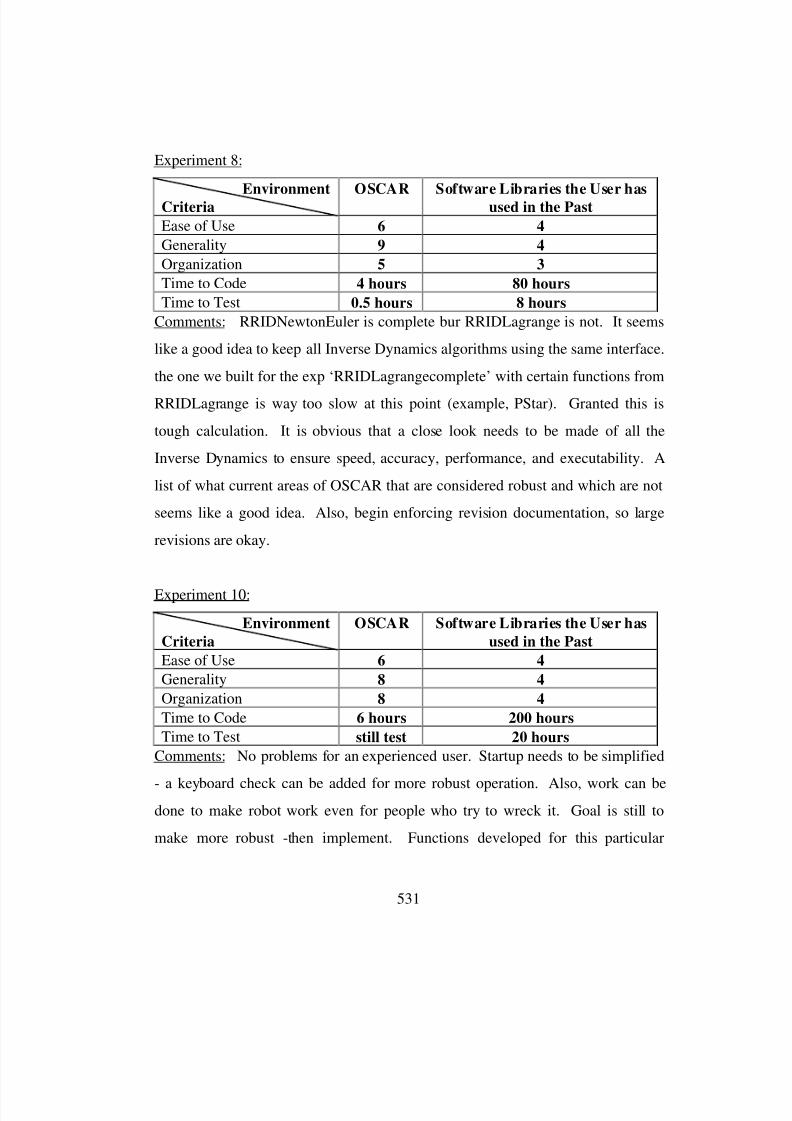
8/3/2019 Chetan Kapoor Dissertation
http://slidepdf.com/reader/full/chetan-kapoor-dissertation 552/612
531
Experiment 8:
EnvironmentCriteria OSCAR Software Libraries the User hasused in the Past
Ease of Use 6 4
Generality 9 4
Organization 5 3
Time to Code 4 hours 80 hours
Time to Test 0.5 hours 8 hours
Comments: RRIDNewtonEuler is complete bur RRIDLagrange is not. It seems
like a good idea to keep all Inverse Dynamics algorithms using the same interface.
the one we built for the exp ‘RRIDLagrangecomplete’ with certain functions from
RRIDLagrange is way too slow at this point (example, PStar). Granted this is
tough calculation. It is obvious that a close look needs to be made of all the
Inverse Dynamics to ensure speed, accuracy, performance, and executability. A
list of what current areas of OSCAR that are considered robust and which are not
seems like a good idea. Also, begin enforcing revision documentation, so large
revisions are okay.
Experiment 10:
Environment
Criteria
OSCAR Software Libraries the User has
used in the Past
Ease of Use 6 4
Generality 8 4
Organization 8 4
Time to Code 6 hours 200 hours
Time to Test still test 20 hours
Comments: No problems for an experienced user. Startup needs to be simplified
- a keyboard check can be added for more robust operation. Also, work can be
done to make robot work even for people who try to wreck it. Goal is still to
make more robust -then implement. Functions developed for this particular
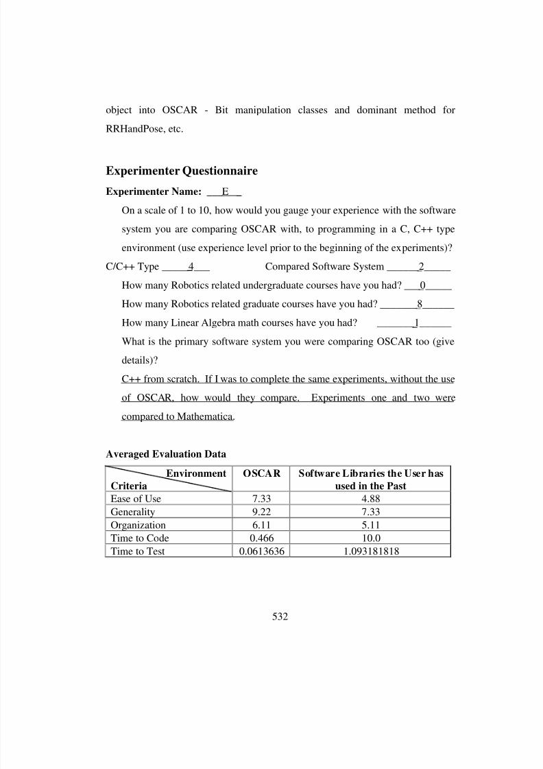
8/3/2019 Chetan Kapoor Dissertation
http://slidepdf.com/reader/full/chetan-kapoor-dissertation 553/612
532
object into OSCAR - Bit manipulation classes and dominant method for
RRHandPose, etc.
Experimenter Questionnaire
Experimenter Name: ___E _
On a scale of 1 to 10, how would you gauge your experience with the software
system you are comparing OSCAR with, to programming in a C, C++ type
environment (use experience level prior to the beginning of the experiments)?
C/C++ Type _____4___ Compared Software System ______2_____ How many Robotics related undergraduate courses have you had? ___0_____
How many Robotics related graduate courses have you had? _______8______
How many Linear Algebra math courses have you had? _______1______
What is the primary software system you were comparing OSCAR too (give
details)?
C++ from scratch. If I was to complete the same experiments, without the use
of OSCAR, how would they compare. Experiments one and two were
compared to Mathematica.
Averaged Evaluation Data
Environment
Criteria
OSCAR Software Libraries the User has
used in the Past
Ease of Use 7.33 4.88
Generality 9.22 7.33
Organization 6.11 5.11
Time to Code 0.466 10.0Time to Test 0.0613636 1.093181818

8/3/2019 Chetan Kapoor Dissertation
http://slidepdf.com/reader/full/chetan-kapoor-dissertation 554/612
533
C.7.6. Experimenter F
Experiment 1:
Environment
Criteria
OSCAR Software Libraries the User has
used in the Past
Ease of Use 9 10
Generality 10 9
Organization 9 10
Time to Code 1.5 hours 0.15 hours
Time to Test 1 hour 0.15 hours
Comments: The math classes structure provided in OSCAR is an excellent
starting point. The Vector and Matrix classes make it easy to do basic linear
algebra computations while the more specific derived classes are extremely useful
as well. The matrix class could have more comments in the code.
Experiment 2:
Environment
Criteria
OSCAR Software Libraries the User has
used in the Past
Ease of Use 9 10
Generality 10 9Organization 9 10
Time to Code 1 hour 0.15 hour
Time to Test 1 hour 0.15 hour
Comments: The robotics specific Xform, rotation, and handpose classes work
well and are very easy to use.
Experiment 3:
Environment
Criteria
OSCAR Software Libraries the User has
used in the Past
Ease of Use 9 9Generality 10 9
Organization 9 8
Time to Code 1 hour 7 hours
Time to Test 1 hour 3 hours

8/3/2019 Chetan Kapoor Dissertation
http://slidepdf.com/reader/full/chetan-kapoor-dissertation 555/612
534
Comments: Forward Kinematics at the position, velocity, and acceleration-level
is simple to use and fairly straight forward. OSCAR at this time provides all the
basics in the area and can easily be expanded as the need for more specialized
modules arises.
Experiment 4:
Environment
Criteria
OSCAR Software Libraries the User has
used in the Past
Ease of Use 9 9
Generality 10 9
Organization 9 8
Time to Code 0.5 hours 6 hours
Time to Test 1 hour 3 hours
Comments:
Experiment 5:
Environment
Criteria
OSCAR Software Libraries the User has
used in the Past
Ease of Use 8 9
Generality 10 9
Organization 8 9
Time to Code 5 hours 8 hours
Time to Test 5 hours 4 hours
Comments: Inverse Kinematics is easy to use once the user figures out how the
software components are structured. The files in this directory could especially
benefit from a readme file outlining the overall layout of the inverse kinematics.
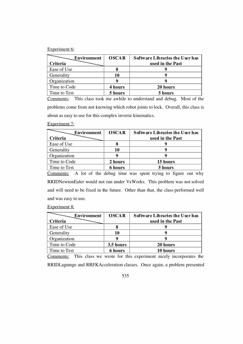
8/3/2019 Chetan Kapoor Dissertation
http://slidepdf.com/reader/full/chetan-kapoor-dissertation 556/612
535
Experiment 6:
EnvironmentCriteria OSCAR Software Libraries the User hasused in the Past
Ease of Use 8 9
Generality 10 9
Organization 9 9
Time to Code 4 hours 20 hours
Time to Test 5 hours 5 hours
Comments: This class took me awhile to understand and debug. Most of the
problems come from not knowing which robot joints to lock. Overall, this class is
about as easy to use for this complex inverse kinematics.
Experiment 7:
Environment
Criteria
OSCAR Software Libraries the User has
used in the Past
Ease of Use 8 9
Generality 10 9
Organization 9 9
Time to Code 2 hours 15 hours
Time to Test 6 hours 5 hours
Comments: A lot of the debug time was spent trying to figure out why
RRIDNewtonEuler would not run under VxWorks. This problem was not solved
and will need to be fixed in the future. Other than that, the class performed well
and was easy to use.
Experiment 8:
Environment
Criteria
OSCAR Software Libraries the User has
used in the Past
Ease of Use 8 9
Generality 10 9
Organization 9 9Time to Code 3.5 hours 20 hours
Time to Test 6 hours 10 hours
Comments: This class we wrote for this experiment nicely incorporates the
RRIDLagrange and RRFKAcceleration classes. Once again, a problem presented

8/3/2019 Chetan Kapoor Dissertation
http://slidepdf.com/reader/full/chetan-kapoor-dissertation 557/612
536
itself when trying to use VxWorks. Also, the Pstar calculations take so much
time that this method is practically worthless for real-time use. I have not written
a great deal of new code. However, I have been working on updating old code,
etc. Overall, OSCAR has provided an excellent structure for writing robotics
code.
Experimenter Questionnaire
Experimenter Name: ___F _
On a scale of 1 to 10, how would you gauge your experience with the software
system you are comparing OSCAR with, to programming in C/C++ type
environment (use experience level prior to the beginning of the experiments)?
C/C++ Type _____1___ Compared Software System ______9 _____
How many Robotics related undergraduate courses have you had? ___1_____
How many Robotics related graduate courses have you had? _______3______
How many Linear Algebra math courses have you had? _______1______
What is the primary software system you were comparing OSCAR too (give
details)?
Matlab. I have written a lot of robotics related code in Matlab and am quite
familiar with all aspects of Matlab programming.
compared to Mathematica.
Averaged Evaluation Data
Environment
Criteria
OSCAR Software Libraries the User has
used in the Past
Ease of Use 8.5 9.25
Generality 10 9
Organization 8.875 9Time to Code 2.48 10.0
Time to Test 3.398692 3.960784314
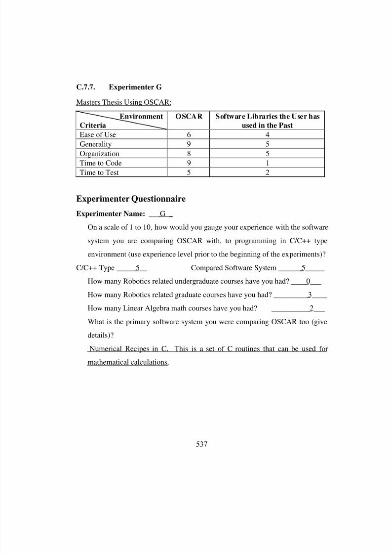
8/3/2019 Chetan Kapoor Dissertation
http://slidepdf.com/reader/full/chetan-kapoor-dissertation 558/612
537
C.7.7. Experimenter G
Masters Thesis Using OSCAR:
Environment
Criteria
OSCAR Software Libraries the User has
used in the Past
Ease of Use 6 4
Generality 9 5
Organization 8 5
Time to Code 9 1
Time to Test 5 2
Experimenter Questionnaire
Experimenter Name: ___G _
On a scale of 1 to 10, how would you gauge your experience with the software
system you are comparing OSCAR with, to programming in C/C++ type
environment (use experience level prior to the beginning of the experiments)?
C/C++ Type _____5__ Compared Software System ______5_____
How many Robotics related undergraduate courses have you had? ____0___
How many Robotics related graduate courses have you had? _________3____
How many Linear Algebra math courses have you had? __________2___
What is the primary software system you were comparing OSCAR too (give
details)?
Numerical Recipes in C. This is a set of C routines that can be used for
mathematical calculations.
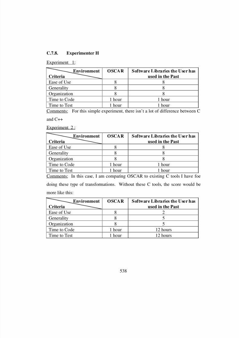
8/3/2019 Chetan Kapoor Dissertation
http://slidepdf.com/reader/full/chetan-kapoor-dissertation 559/612
538
C.7.8. Experimenter H
Experiment 1:
Environment
Criteria
OSCAR Software Libraries the User has
used in the Past
Ease of Use 8 8
Generality 8 8
Organization 8 8
Time to Code 1 hour 1 hour
Time to Test 1 hour 1 hour
Comments: For this simple experiment, there isn’t a lot of difference between C
and C++
Experiment 2 :
Environment
Criteria
OSCAR Software Libraries the User has
used in the Past
Ease of Use 8 8
Generality 8 8
Organization 8 8
Time to Code 1 hour 1 hour
Time to Test 1 hour 1 hour
Comments: In this case, I am comparing OSCAR to existing C tools I have foedoing these type of transformations. Without these C tools, the score would be
more like this:
Environment
Criteria
OSCAR Software Libraries the User has
used in the Past
Ease of Use 8 2
Generality 8 5
Organization 8 5
Time to Code 1 hour 12 hours
Time to Test 1 hour 12 hours
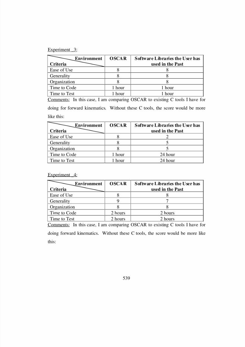
8/3/2019 Chetan Kapoor Dissertation
http://slidepdf.com/reader/full/chetan-kapoor-dissertation 560/612
539
Experiment _3:
EnvironmentCriteria OSCAR Software Libraries the User hasused in the Past
Ease of Use 8 8
Generality 8 8
Organization 8 8
Time to Code 1 hour 1 hour
Time to Test 1 hour 1 hour
Comments: In this case, I am comparing OSCAR to existing C tools I have for
doing for forward kinematics. Without these C tools, the score would be more
like this:
Environment
Criteria
OSCAR Software Libraries the User has
used in the Past
Ease of Use 8 2
Generality 8 5
Organization 8 5
Time to Code 1 hour 24 hour
Time to Test 1 hour 24 hour
Experiment _4:
EnvironmentCriteria
OSCAR Software Libraries the User hasused in the Past
Ease of Use 8 8
Generality 9 7
Organization 8 8
Time to Code 2 hours 2 hours
Time to Test 2 hours 2 hours
Comments: In this case, I am comparing OSCAR to existing C tools I have for
doing forward kinematics. Without these C tools, the score would be more like
this:
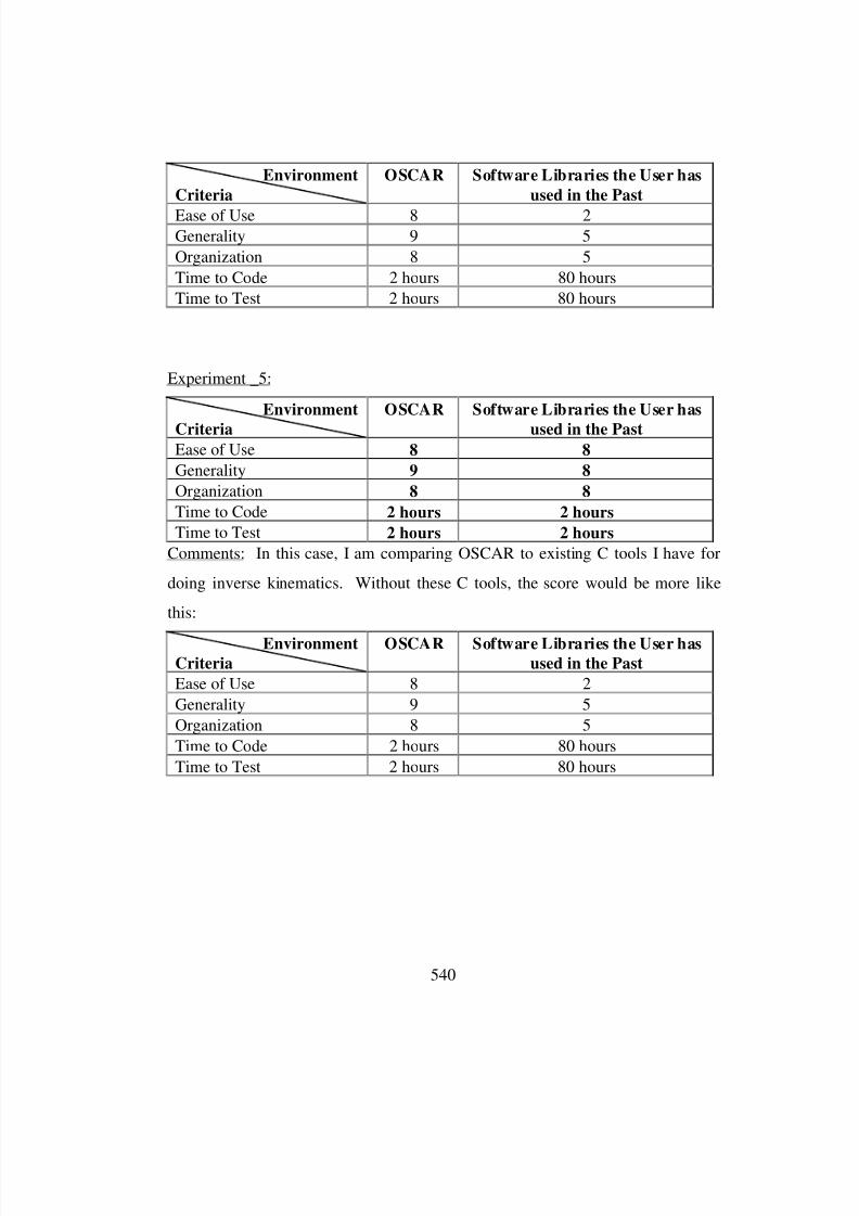
8/3/2019 Chetan Kapoor Dissertation
http://slidepdf.com/reader/full/chetan-kapoor-dissertation 561/612
540
Environment
Criteria
OSCAR Software Libraries the User has
used in the Past
Ease of Use 8 2Generality 9 5
Organization 8 5
Time to Code 2 hours 80 hours
Time to Test 2 hours 80 hours
Experiment _5:
Environment
Criteria
OSCAR Software Libraries the User has
used in the PastEase of Use 8 8
Generality 9 8
Organization 8 8
Time to Code 2 hours 2 hours
Time to Test 2 hours 2 hours
Comments: In this case, I am comparing OSCAR to existing C tools I have for
doing inverse kinematics. Without these C tools, the score would be more like
this:
EnvironmentCriteria
OSCAR Software Libraries the User hasused in the Past
Ease of Use 8 2
Generality 9 5
Organization 8 5
Time to Code 2 hours 80 hours
Time to Test 2 hours 80 hours
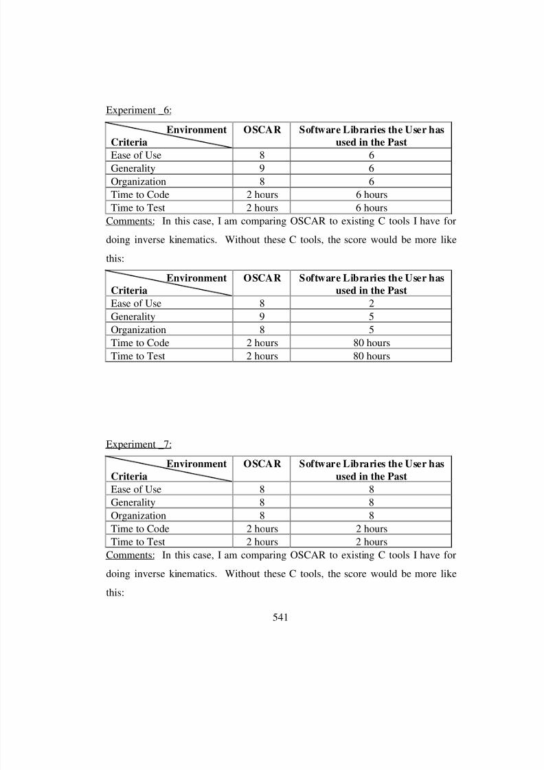
8/3/2019 Chetan Kapoor Dissertation
http://slidepdf.com/reader/full/chetan-kapoor-dissertation 562/612
541
Experiment _6:
EnvironmentCriteria OSCAR Software Libraries the User hasused in the Past
Ease of Use 8 6
Generality 9 6
Organization 8 6
Time to Code 2 hours 6 hours
Time to Test 2 hours 6 hours
Comments: In this case, I am comparing OSCAR to existing C tools I have for
doing inverse kinematics. Without these C tools, the score would be more like
this:
Environment
Criteria
OSCAR Software Libraries the User has
used in the Past
Ease of Use 8 2
Generality 9 5
Organization 8 5
Time to Code 2 hours 80 hours
Time to Test 2 hours 80 hours
Experiment _7:
Environment
Criteria
OSCAR Software Libraries the User has
used in the Past
Ease of Use 8 8
Generality 8 8
Organization 8 8
Time to Code 2 hours 2 hours
Time to Test 2 hours 2 hoursComments: In this case, I am comparing OSCAR to existing C tools I have for
doing inverse kinematics. Without these C tools, the score would be more like
this:
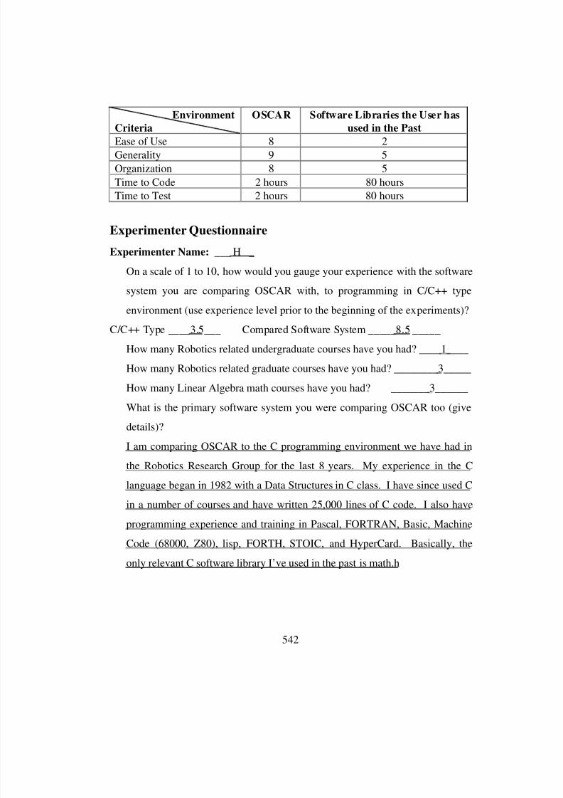
8/3/2019 Chetan Kapoor Dissertation
http://slidepdf.com/reader/full/chetan-kapoor-dissertation 563/612
542
Environment
Criteria
OSCAR Software Libraries the User has
used in the Past
Ease of Use 8 2Generality 9 5
Organization 8 5
Time to Code 2 hours 80 hours
Time to Test 2 hours 80 hours
Experimenter Questionnaire
Experimenter Name: ___ H _
On a scale of 1 to 10, how would you gauge your experience with the software
system you are comparing OSCAR with, to programming in C/C++ type
environment (use experience level prior to the beginning of the experiments)?
C/C++ Type ____3.5___ Compared Software System _____8.5 _____
How many Robotics related undergraduate courses have you had? ____1____
How many Robotics related graduate courses have you had? ________3_____
How many Linear Algebra math courses have you had? _______3______
What is the primary software system you were comparing OSCAR too (give
details)?
I am comparing OSCAR to the C programming environment we have had in
the Robotics Research Group for the last 8 years. My experience in the C
language began in 1982 with a Data Structures in C class. I have since used C
in a number of courses and have written 25,000 lines of C code. I also have
programming experience and training in Pascal, FORTRAN, Basic, Machine
Code (68000, Z80), lisp, FORTH, STOIC, and HyperCard. Basically, the
only relevant C software library I’ve used in the past is math.h

8/3/2019 Chetan Kapoor Dissertation
http://slidepdf.com/reader/full/chetan-kapoor-dissertation 564/612
543
Averaged Evaluation Data
Environment
Criteria
OSCAR Software Libraries the User has
used in the Past
Ease of Use 8 7.7
Generality 8.43 7.571
Organization 8.0 7.7
Time to Code 7.33 10.0
Time to Test 7.33 10.0
8/3/2019 Chetan Kapoor Dissertation
http://slidepdf.com/reader/full/chetan-kapoor-dissertation 565/612
544
Appendix D
D. Class Libraries for 3D Procedural Modeling
D.1. Introduction
The purpose of this project was to develop object-oriented libraries that
would assist the applications developer in generating and rendering various 3D
shapes. The goal as specified was to provide a class structure that would allow
the creation of various 3D shapes like cones, cylinders, disks, etc. Other desired
capability of these libraries was to provide the user with various rendering options
(WIREFRAME, SMOOTH, FACETED) and shaded surface options (INSIDE,
OUTSIDE, BOTHSIDE). In addition, an environment had to be provided in
which the user defined scene could be rendered. Also, to these graphics specific
classes, other support classes, like container classes were also to be provided.
After completion of these libraries it was required to develop an application that
demonstrated the use of these libraries. This software was to be developed on a
Silicon Graphics UNIX workstation using the GL libraries. These libraries are
now also available on Windows NT using OpenGL.The following paragraphs describe the class structure of these libraries.
The individual classes, their interface, connectivity, and usage is described below.
8/3/2019 Chetan Kapoor Dissertation
http://slidepdf.com/reader/full/chetan-kapoor-dissertation 566/612
545
Overall, 5400 lines of C++ code was written and a 800 line application was
developed using these libraries.
D.2. Mathematical Classes
D.2.1. Class Matrix
This class was imported from National Institute of Health Class Library
(NIHCL) collection. Various changes were made to this class, methods were
added and some bugs were fixed. The class implements the Matrix data type and
is fairly intuitive. Methods for inversion, determinant calculation, and
multiplication were re-implemented for speed and accuracy. Along with the
Matrix class the classes MatrixCol, and MatrixRow are declared. These classes
are used to access specific rows and columns of a Matrix. The interface to this
class is present in the header file Rmath.h (see Section D.5.1).
D.2.2. Class TransformMatrix : public Matrix
This class was derived from the Matrix class and basically implements a 4
by 4 homogenous transformation matrix. The purpose of the inheritance was to
achieve restriction and extension. The restriction was achieved by limiting the
Matrix class to 4 by 4 and the extension was achieved by redefining the methods
for multiplication (for speed ) and also by adding methods which would convert a
TransformMatrix into its Euler angle or Fixed angle representation. The
declaration of this class is specified in Rmath.h (see Section D.5.1).
D.2.3. Class Vector
This class implements an abstraction for a one dimensional array. It has
methods for multiplication of the vector with matrices, etc. The declaration of
this class is specified in the Rmath.h file (see Section D.5.1).
8/3/2019 Chetan Kapoor Dissertation
http://slidepdf.com/reader/full/chetan-kapoor-dissertation 567/612
546
D.2.4. Class Tensor
This class implements a 3D vector and is essentially an array of matrices.Methods for this class allow the user to access elements, rows, columns, or
matrices from this 3D vector. The declaration of this class is specified in the
Rmath.h file (see Section D.5.1).
D.3. Geometry Related Classes
These classes implement geometric primitives that form the basic
primitives of a geometric modeling system. The classes implemented are Point
and Vector3D.
D.3.1. Class Point
This class implements an abstract data type that specifies a 3D point in
space. Various homogenous transformations can be applied to these points.
These include translation, scaling, and rotation about any desired axis. A point
can also be extruded along a specified vector for a certain length. The class
declaration for Point is given in the file Draw.h ( see Section D.5.2).
D.3.2. Class Vector3D : public Vector
This class Vector3D is implemented as an inheritance of the Vector class.
This class is a restriction and an extension of the Vector class. The restriction is
applied by constraining the Vector class to length three. The extension is applied
by adding methods for calculating the cross-product, dot product, normals, etc.
The class declaration is given in the Draw.h file (see Section D.5.2).

8/3/2019 Chetan Kapoor Dissertation
http://slidepdf.com/reader/full/chetan-kapoor-dissertation 568/612
547
D.3.3. Class Polygon
This class implements a basic drawing primitive. The input parameter tothis class is an array of points. These points are used to generate a polygon. The
normal is calculated based on the points supplied. To create a polygon whose
normal faces outside (e.g., coming out of the plane of the towards the user), the
points should be supplied in counter-clockwise direction. This is illustrated in
Figure D.1.
Point 1
Point 2
Point 3
Point 4
Point 5
Normal in + z
Y
Figure D.1: Normal Calculation for a Polygon.
If the vertices are supplied in clockwise direction the normal calculated
faces in the other direction. When rendering a polygon, the user can pick between
WIREFRAME and SHADED. Also, the user can pick the desired side of the
polygon for shading. These sides are OUTSIDE and INSIDE. The OUTSIDE
side is the side for which the normal was calculated assuming counter-clockwise
specification of vertices. The Polygon class forms the basic building block of all
shapes that are created using procedural modeling. The class declaration is
specified in the file Shape.h (see Section D.5.3).
8/3/2019 Chetan Kapoor Dissertation
http://slidepdf.com/reader/full/chetan-kapoor-dissertation 569/612
548
D.3.4. Class Attributes
This class can be thought of as a C structure that holds related data. In thiscase the Attributes class specifies the shading and the rendering characteristics of
a geometric shape. The shading characteristic can be INSIDE or OUTSIDE. This
specifies the side of a shape that gets shaded. The rendering characteristic can be
WIREFRAME, FACETED, or SMOOTH.
D.3.5. Class Shape
This class specifies an abstract data type that acts as the base class of all
possible 3D shapes. Specific shape classes are derived from this class. The key
members of this class are the ’number of polygons’, an ’array of polygons’ of which
make up the shape, and the ’attributes’ of this shape, and the ’origin’ of this shape
which is an instantiation of a Point. The origin member can later be used to add
bounding-volume capability to the Shape class. There are two public members
for setting the attributes of the Shape class. There is virtual method called Draw()
which is used to render the shape in the environment.
Here it is seen that rendering is a part of the Shape class. This is done
because these libraries are not intended for distributed use. Anyway, these
libraries can be easily ported by redefining the Draw method to be a part of the
Environment. Also, in the whole Shape class hierarchy, it is only the Draw
method that uses GL specific commands.
In the following paragraphs the classes derived from Shape are described.
D.3.6. Class QuadMeshShape : public Shape
This class groups together all objects that are made of quadrilateral strips
of polygons. This class redefines the protected method ’renderSmoothShaded()’ in
a manner such that it works efficiently for quadrilateral strips.
8/3/2019 Chetan Kapoor Dissertation
http://slidepdf.com/reader/full/chetan-kapoor-dissertation 570/612
549
D.3.7. Class TriMeshShape : public Shape
This class groups together all objects that are made of triangular meshes.This class redefines the protected method ’renderSmoothShaded()’ in a manner
such that it works efficiently for triangular meshes.
D.3.8. Class PolyShape : public Shape
This class groups together all objects that are made out of flat polygons
(for i.e. buildings). This class redefines the protected method
’renderSmoothShaded()’ to be the same as ’renderFaceted()’. To draw an object of
type PolyShape, we simply draw the polygons that make up the object.
D.3.9. Class Cylinder : public QuadMeshShape
This class defines the abstract data type Cylinder. The key attributes of
Cylinder are its length and radius.
D.3.10. Class CylinderX : public Cylinder
This defines a cylinder whose axis is along the x-axis.
CylinderX cylx(length, radius, no_of_facets = 10, origin = 0, arcstart =
0.0, arcstop = 360.0);
D.3.11. Class CylinderY : public Cylinder
This defines a cylinder whose axis is along the y-axis.
CylinderY cyly(length, radius, no_of_facets = 10, origin = 0, arcstart =
0.0, arcstop = 360.0);
D.3.12. Class CylinderZ : public Cylinder
This defines a cylinder whose axis is along the z-axis.
CylinderY cylz(length, radius, no_of_facets = 10, origin = 0, arcstart =
0.0, arcstop = 360.0);

8/3/2019 Chetan Kapoor Dissertation
http://slidepdf.com/reader/full/chetan-kapoor-dissertation 571/612
550
D.3.13. Class TruncCone : public QuadMeshShape
This class defines the abstract data type for a truncated cone. The keyattributes of TruncCone are its length, lower radius, and upper radius.
D.3.14. Class TruncConeX : public TruncCone
This defines a truncated cone whose axis is along the x-axis.
TruncConeX tcx(length, radius1, radius2, no_of_facets = 10, origin = 0,
arcstart = 0.0, arcstop = 360.0);
D.3.15. Class TruncConeY : public TruncCone
This defines a truncated cone whose axis is along the y-axis.
TruncConeY tcy(length, radius1, radius2, no_of_facets = 10, origin = 0,
arcstart = 0.0, arcstop = 360.0);
D.3.16. Class TruncConeZ : public TruncCone
This defines a truncated cone whose axis is along the z-axis.
TruncConeZ tcz(length, radius1, radius2, no_of_facets = 10, origin = 0,
arcstart = 0.0, arcstop = 360.0);
D.3.17. Class Extrusion : public QuadMeshShape
This class defines all shapes that are made by extruding a set of points in a
given direction for a specified length. The points should be specified in counter-
clockwise direction if the user is looking down at the cross-section from the
direction in which the extrusion is to take place. For example, to extrude an I-
Beam, the points are specified as shown in Figure D.2. In this case it is assumed
that the extrusion direction will be out of the page towards the user. If the
extrusion has to take place into the page, then the points should be specified in
clockwise direction. However, in the event of the points not being specified in the
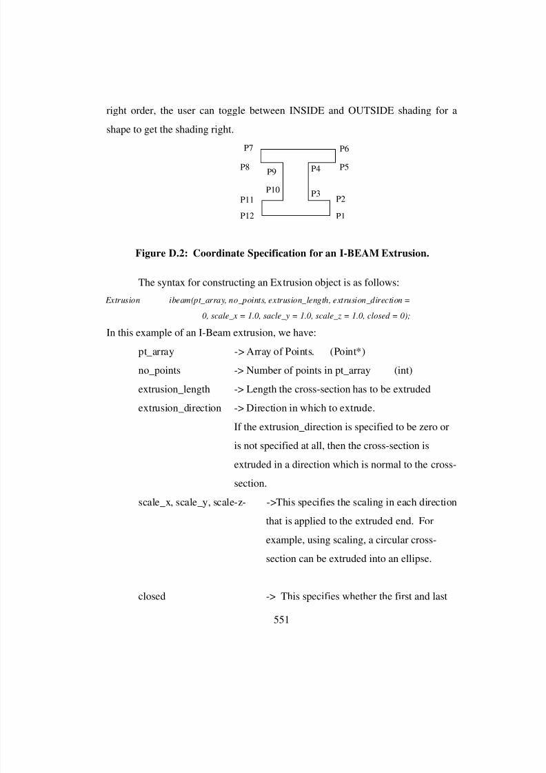
8/3/2019 Chetan Kapoor Dissertation
http://slidepdf.com/reader/full/chetan-kapoor-dissertation 572/612
551
right order, the user can toggle between INSIDE and OUTSIDE shading for a
shape to get the shading right.
P1
P5P4
P3P2
P6P7
P8P9
P10P11
P12
Figure D.2: Coordinate Specification for an I-BEAM Extrusion.
The syntax for constructing an Extrusion object is as follows:
Extrusion ibeam(pt_array, no_points, extrusion_length, extrusion_direction =
0, scale_x = 1.0, sacle_y = 1.0, scale_z = 1.0, closed = 0);
In this example of an I-Beam extrusion, we have:
pt_array -> Array of Points. (Point*)
no_points -> Number of points in pt_array (int)
extrusion_length -> Length the cross-section has to be extruded
extrusion_direction -> Direction in which to extrude.
If the extrusion_direction is specified to be zero or
is not specified at all, then the cross-section is
extruded in a direction which is normal to the cross-
section.
scale_x, scale_y, scale-z- ->This specifies the scaling in each direction
that is applied to the extruded end. For
example, using scaling, a circular cross-section can be extruded into an ellipse.
closed -> This specifies whether the first and last

8/3/2019 Chetan Kapoor Dissertation
http://slidepdf.com/reader/full/chetan-kapoor-dissertation 573/612
552
points of the cross-section are joined
together or not. The default for this in ’not
joined’. A value of ’1’ makes the cross-
section closed.
D.3.18. Class Sweep : public QuadMeshShape
This class defines all shapes that are formed by rotating a set of points
about any specified axis. The points should be specified in counter-clockwise
direction if the user is looking down at the cross-section from the direction
opposite to which the sweep is to take place. However, in the event of the points
not being specified in the right order, the user can toggle between INSIDE and
OUTSIDE shading for a shape to get the shading right.
The syntax for constructing a Sweep object is as follows:
Sweep ibeam(pt_array, no_points, no_facets = 10, axis = 0, double arcstart = 0.0,
double arcstop = 360.0, closed = 0);
In this example of an I-Beam sweep, we have:
pt_array -> Array of Points. (Point*)
no_points -> Number of points in pt_array (int)
no_facets -> Number of facets to divide the sweep into
axis -> Direction of axis about which to sweep
If the sweep axis is specified to be zero or is not
specified at all, then the cross-section is swept about
the y-axis.
arcstart Value of the angle at which to start the sweep
arcstop Value of the angle at which to stop the sweep
closed -> This specifies whether the first and last points of
the cross-section are same or not. If the points are
8/3/2019 Chetan Kapoor Dissertation
http://slidepdf.com/reader/full/chetan-kapoor-dissertation 574/612
553
same, then a 1 should be specified. This
information helps in the smooth shading of the
sweep.
D.3.19. Class Cone : public TriMeshShape
This class defines the abstract data type for a cone. The key attributes of
Cone are its height and radius.
D.3.20. Class ConeX : public Cone
This defines a cone whose axis is along the x-axis.ConeX conex(height, radius, no_of_facets = 10, origin = 0, arcstart = 0.0,
arcstop = 360.0);
D.3.21. Class ConeY : public Cone
This defines a cone whose axis is along the y-axis.
ConeY coney(height, radius, no_of_facets = 10, origin = 0, arcstart = 0.0,
arcstop = 360.0);
D.3.22. Class ConeZ : public Cone
This defines a cone whose axis is along the z-axis.
ConeZ conez(height, radius, no_of_facets = 10, origin = 0, arcstart = 0.0,
arcstop = 360.0);
D.3.23. Class Disk : public TriMeshShape
This class defines the abstract data type for a planar disk. The key
attribute of a Disk is its radius.
D.3.24. Class DiskX : public Disk
This defines a disk who’s normal is along the x-axis.
8/3/2019 Chetan Kapoor Dissertation
http://slidepdf.com/reader/full/chetan-kapoor-dissertation 575/612
554
DiskX diskz(radius, no_of_facets = 10, origin = 0, arcstart = 0.0, arcstop = 360.0);
D.3.25. Class DiskY : public Disk
This defines a disk who’s normal is along the y-axis.
DiskY diaky( radius, no_of_facets = 10, origin = 0, arcstart = 0.0, arcstop = 360.0);
D.3.26. Class DiskZ : public Disk
This defines a disk who’s normal is along the z-axis.
DiskZ diskz(radius, no_of_facets = 10, origin = 0, arcstart = 0.0, arcstop = 360.0);
D.3.27. Class Box : public PolyShape
This defines a 3D box about a specified origin.
Box box(length_x, height_y, depth_z, origin = 0);
D.4. Class Diagrams
The class diagrams for the software developed for this project are given
below. The notation proposed by Booch [1994] is used for these class diagrams.
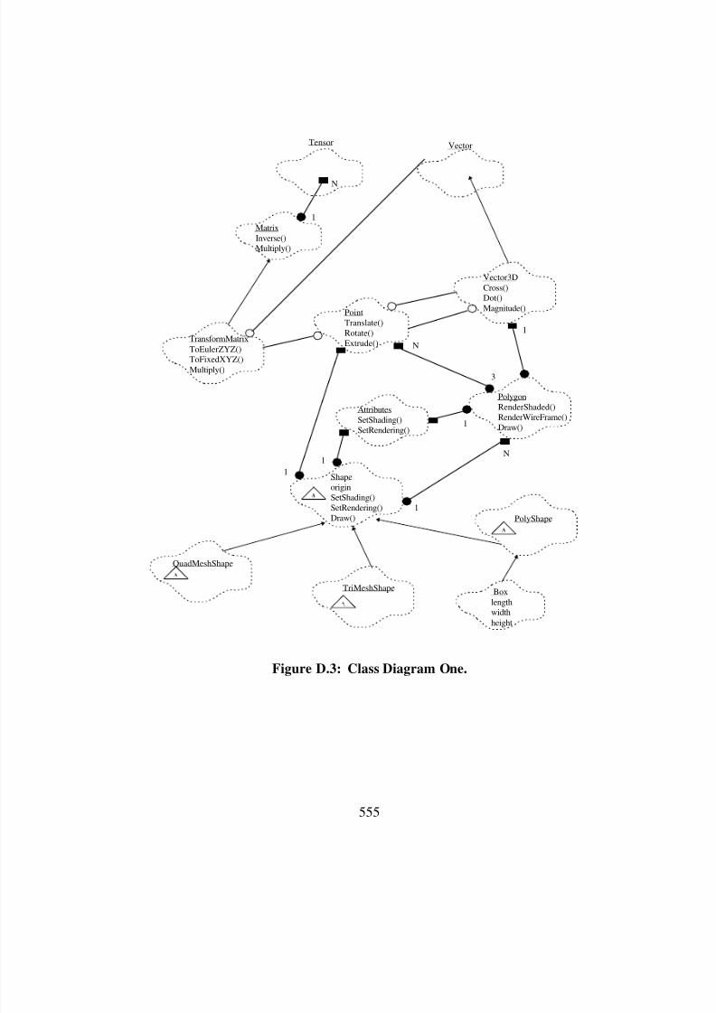
8/3/2019 Chetan Kapoor Dissertation
http://slidepdf.com/reader/full/chetan-kapoor-dissertation 576/612
555
MatrixInverse()Multiply()
TransformMatrixToEulerZYZ()ToFixedXYZ()Multiply()
Vector
Vector3DCross()Dot()Magnitude()
Tensor
PointTranslate()Rotate()Extrude()
AttributesSetShading()SetRendering()
PolygonRenderShaded()RenderWireFrame()Draw()
ShapeoriginSetShading()SetRendering()Draw()
QuadMeshShape
PolyShape
TriMeshShape
N
1
Boxlengthwidthheight
1
3
N
1
1
N1
1
Figure D.3: Class Diagram One.
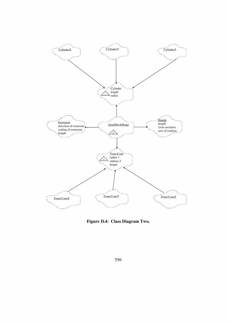
8/3/2019 Chetan Kapoor Dissertation
http://slidepdf.com/reader/full/chetan-kapoor-dissertation 577/612
556
TruncConeradius 1
raduius 2heignt
Cylinderlengthradius
QuadMeshShape
CylinderZ
Sweep
lengthcross-sectiuonaxis of rotation
CylinderYCylinderX
TruncConeZTruncConeYTruncConeX
Extrusiondirection of extrusionscaling of extrusionlength
Figure D.4: Class Diagram Two.
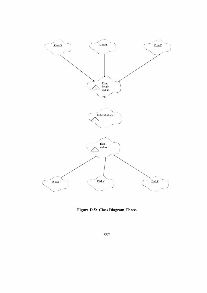
8/3/2019 Chetan Kapoor Dissertation
http://slidepdf.com/reader/full/chetan-kapoor-dissertation 578/612
557
Disk
radius
Coneheight
radius
TriMeshShape
ConeZConeYConeX
DiskZDiskYDiskX
Figure D.5: Class Diagram Three.
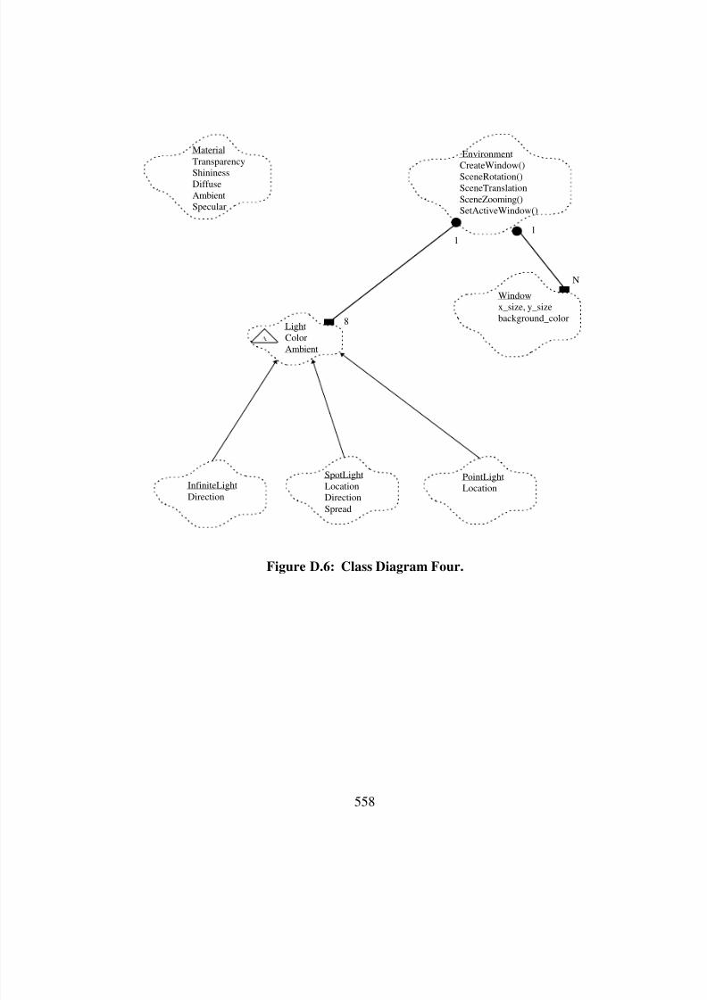
8/3/2019 Chetan Kapoor Dissertation
http://slidepdf.com/reader/full/chetan-kapoor-dissertation 579/612
558
LightColor
Ambient
InfiniteLight
Direction
PointLightLocation
SpotLightLocationDirection
Spread
Material
Transparency
ShininessDiffuseAmbientSpecular
EnvironmentCreateWindow()
SceneRotation()SceneTranslationSceneZooming()SetActiveWindow()
Windowx_size, y_sizebackground_color
N
11
8
Figure D.6: Class Diagram Four.
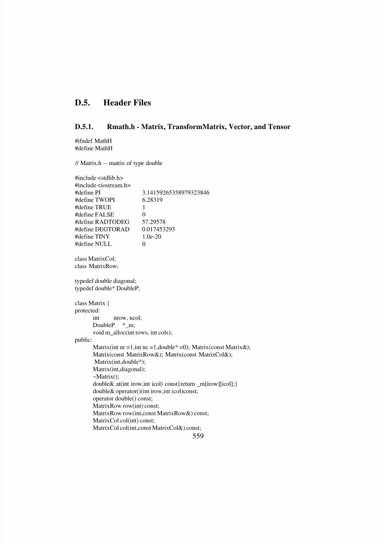
8/3/2019 Chetan Kapoor Dissertation
http://slidepdf.com/reader/full/chetan-kapoor-dissertation 580/612
559
D.5. Header Files
D.5.1. Rmath.h - Matrix, TransformMatrix, Vector, and Tensor
#ifndef MathH#define MathH
// Matrix.h -- matrix of type double
#include <stdlib.h>#include <iostream.h>
#define PI 3.14159265358979323846#define TWOPI 6.28319#define TRUE 1#define FALSE 0#define RADTODEG 57.29578#define DEGTORAD 0.017453293#define TINY 1.0e-20#define NULL 0
class MatrixCol;class MatrixRow;
typedef double diagonal;
typedef double* DoubleP;
class Matrix {protected:
int nrow, ncol;DoubleP *_m;void m_alloc(int rows, int cols);
public:Matrix(int nr =1,int nc =1,double* =0); Matrix(const Matrix&);Matrix(const MatrixRow&); Matrix(const MatrixCol&);Matrix(int,double*);
Matrix(int,diagonal);~Matrix();double& at(int irow,int icol) const{return _m[irow][icol];}double& operator()(int irow,int icol)const;operator double() const;MatrixRow row(int) const;MatrixRow row(int,const MatrixRow&) const;MatrixCol col(int) const;MatrixCol col(int,const MatrixCol&) const;
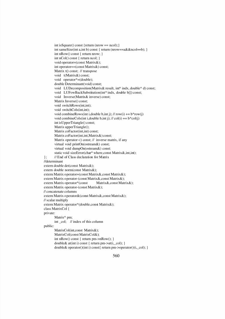
8/3/2019 Chetan Kapoor Dissertation
http://slidepdf.com/reader/full/chetan-kapoor-dissertation 581/612
560
int isSquare() const {return (nrow == ncol);}int sameSize(int a,int b) const { return (nrow==a&&ncol==b); }int nRow() const { return nrow; }int nCol() const { return ncol; }void operator=(const Matrix&);int operator==(const Matrix&) const;Matrix t() const; // transposevoid t(Matrix&) const;void operator*=(double);double Determinant(void) const;void LUDecomposition(Matrix& result, int* indx, double* d) const;void LUFowBackSubstitution(int* indx, double b[]) const;void Inverse(Matrix& inverse) const;Matrix Inverse() const;void switchRows(int,int);void switchCols(int,int);void combineRows(int i,double b,int j); // row(i) += b*row(j)void combineCols(int i,double b,int j); // col(i) += b*col(j)int isUpperTriangle() const;Matrix upperTriangle();Matrix coFactor(int,int) const;Matrix coFactor(int,int,Matrix&) const;Matrix operator~() const; // inverse matrix, if anyvirtual void printOn(ostream&) const;virtual void dumpOn(ostream&) const;static void sizeError(char* where,const Matrix&,int,int);
}; // End of Class declaration for Matrix //determinantextern double det(const Matrix&);extern double norm(const Matrix&);extern Matrix operator+(const Matrix&,const Matrix&);extern Matrix operator-(const Matrix&,const Matrix&);extern Matrix operator*(const Matrix&,const Matrix&);extern Matrix operator-(const Matrix&); // concatenate columnsextern Matrix operator&(const Matrix&,const Matrix&); // scalar multiplyextern Matrix operator*(double,const Matrix&);class MatrixCol {private:
Matrix* pm;int _col; // index of this column
public:MatrixCol(int,const Matrix&);MatrixCol(const MatrixCol&);int nRow() const { return pm->nRow(); }double& at(int i) const { return pm->at(i,_col); }double& operator()(int i) const{ return pm->operator()(i,_col); }

8/3/2019 Chetan Kapoor Dissertation
http://slidepdf.com/reader/full/chetan-kapoor-dissertation 582/612
561
void operator=(const MatrixCol&);void operator+=(const MatrixCol&);virtual void printOn(ostream&) const;
}; // End of class declaraion of MatrixColclass MatrixRow {private:
Matrix* pm;int _row; // index of this row
public:MatrixRow(int,const Matrix&);MatrixRow(const MatrixRow&);int nCol() const { return pm->nCol(); }double& at(int i) const { return pm->at(_row,i); }double& operator()(int i) const { return pm->operator()(_row,i); }double operator^(const MatrixCol&) const; // dot productvoid operator=(const MatrixRow&);virtual void printOn(ostream&) const;
}; // End of class declaration of MatrixRowextern ostream& operator<<(ostream& strm,const Matrix& m);extern ostream& operator<<(ostream& strm,const MatrixRow& m);extern ostream& operator<<(ostream& strm,const MatrixCol& m);
// class declaraton for Vectorclass Vector {protected:
int size;double *element;void init(int, const double *);
public:Vector(int sz) { init(sz, 0); }Vector(int sz, const double* array) { init(sz,array); }Vector(const Vector& v) { init(v.size, v.element); }~Vector() { delete [] element;}int GetSize() const{ return size;}void SetValues(double*) const {}double* GetArray() const {return element;}double GetMagnitude() const;double& at(int index) const {
return element[index];}double& operator[] (int index) const;Vector& operator=(const Vector&);int operator==(const Vector&) const;Vector& operator*=(double);Vector& operator/=(double);Vector& operator+=(double);Vector& operator-=(double);Vector& operator+=(const Vector& v);
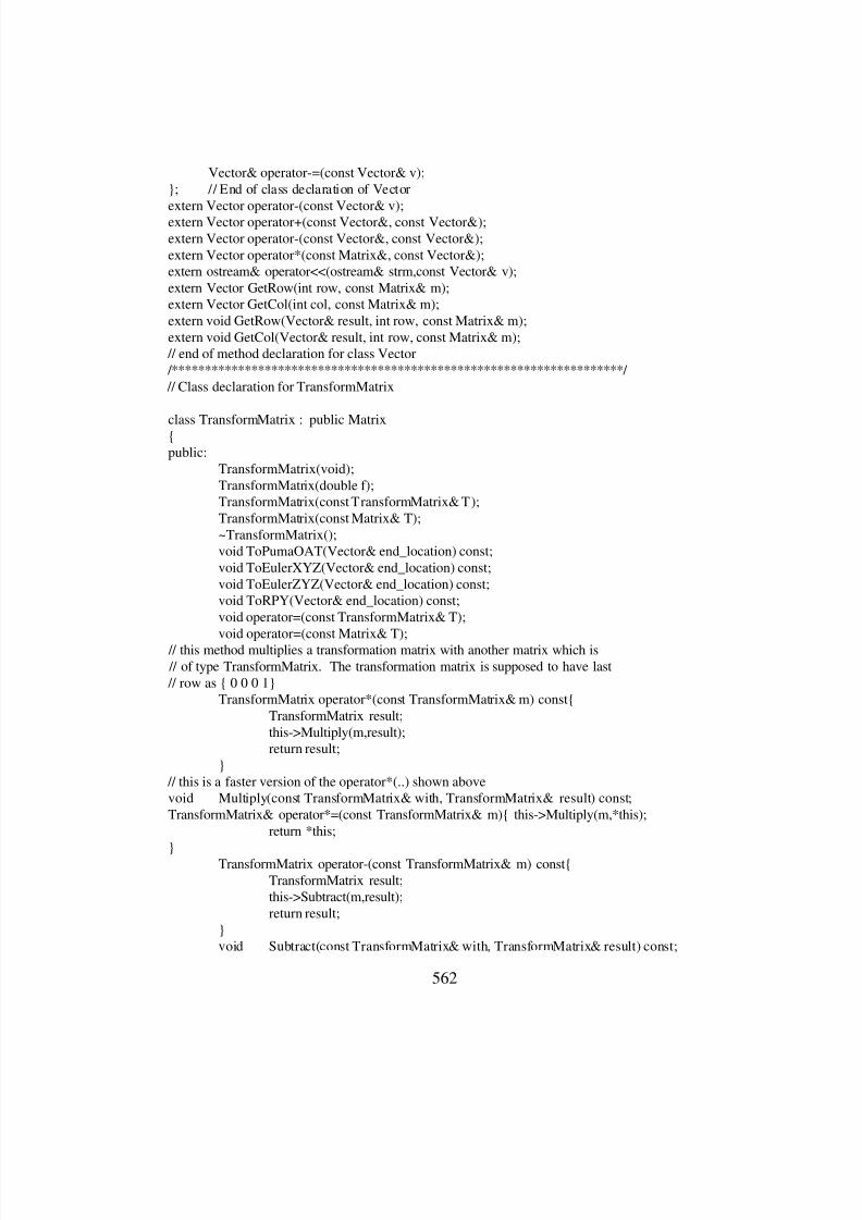
8/3/2019 Chetan Kapoor Dissertation
http://slidepdf.com/reader/full/chetan-kapoor-dissertation 583/612
562
Vector& operator-=(const Vector& v);}; // End of class declaration of Vectorextern Vector operator-(const Vector& v);extern Vector operator+(const Vector&, const Vector&);extern Vector operator-(const Vector&, const Vector&);extern Vector operator*(const Matrix&, const Vector&);extern ostream& operator<<(ostream& strm,const Vector& v);extern Vector GetRow(int row, const Matrix& m);extern Vector GetCol(int col, const Matrix& m);extern void GetRow(Vector& result, int row, const Matrix& m);extern void GetCol(Vector& result, int row, const Matrix& m); // end of method declaration for class Vector /********************************************************************/ // Class declaration for TransformMatrix
class TransformMatrix : public Matrix{public:
TransformMatrix(void);TransformMatrix(double f);TransformMatrix(const TransformMatrix& T);TransformMatrix(const Matrix& T);~TransformMatrix();void ToPumaOAT(Vector& end_location) const;void ToEulerXYZ(Vector& end_location) const;void ToEulerZYZ(Vector& end_location) const;void ToRPY(Vector& end_location) const;void operator=(const TransformMatrix& T);void operator=(const Matrix& T);
// this method multiplies a transformation matrix with another matrix which is // of type TransformMatrix. The transformation matrix is supposed to have last // row as { 0 0 0 1}
TransformMatrix operator*(const TransformMatrix& m) const{TransformMatrix result;this->Multiply(m,result);return result;
} // this is a faster version of the operator*(..) shown abovevoid Multiply(const TransformMatrix& with, TransformMatrix& result) const;TransformMatrix& operator*=(const TransformMatrix& m){ this->Multiply(m,*this);
return *this;}
TransformMatrix operator-(const TransformMatrix& m) const{TransformMatrix result;this->Subtract(m,result);return result;
}void Subtract(const TransformMatrix& with, TransformMatrix& result) const;
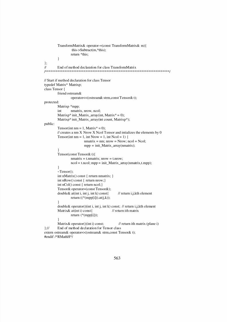
8/3/2019 Chetan Kapoor Dissertation
http://slidepdf.com/reader/full/chetan-kapoor-dissertation 584/612
563
TransformMatrix& operator-=(const TransformMatrix& m){this->Subtract(m,*this);return *this;
}}; // End of method declaration for class TransformMatrix /***********************************************************************/
// Start if method declaration for class Tensortypedef Matrix* Matrixp;class Tensor {
friend ostream&operator<<(ostream& strm,const Tensor& t);
protected:Matrixp *mpp;int nmatrix, nrow, ncol;Matrixp* init_Matrix_array(int, Matrix* = 0);Matrixp* init_Matrix_array(int count, Matrixp*);
public:Tensor(int nm = 1, Matrix* = 0); // creates a nm X Nrow X Ncol Tensor and intializes the elements by 0Tensor(int nm = 1, int Nrow = 1, int Ncol = 1) {
nmatrix = nm; nrow = Nrow; ncol = Ncol;mpp = init_Matrix_array(nmatrix);
}Tensor(const Tensor& t){
nmatrix = t.nmatrix; nrow = t.nrow;ncol = t.ncol; mpp = init_Matrix_array(nmatrix,t.mpp);
}~Tensor();int nMatrix() const { return nmatrix; }int nRow() const { return nrow;}int nCol() const { return ncol;}Tensor& operator=(const Tensor&);double& at(int i, int j, int k) const{ // return i,j,kth element
return ((*(mpp[i])).at(j,k));}double& operator()(int i, int j, int k) const; // return i,j,kth elementMatrix& at(int i) const{ // return ith matrix
return (*(mpp[i]));}Matrix& operator()(int i) const; // return ith matrix (plane i)
};// End of method declaration for Tensor classextern ostream& operator<<(ostream& strm,const Tensor& t);#endif /*RMathH*/
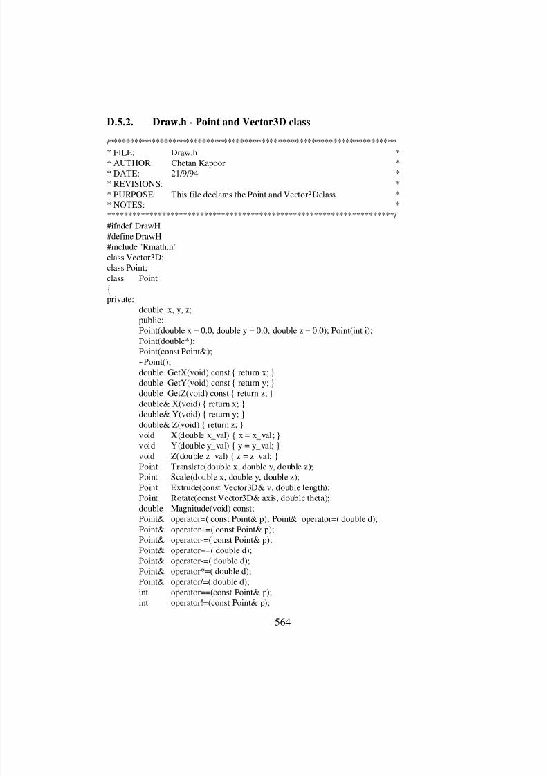
8/3/2019 Chetan Kapoor Dissertation
http://slidepdf.com/reader/full/chetan-kapoor-dissertation 585/612
564
D.5.2. Draw.h - Point and Vector3D class
/********************************************************************* FILE: Draw.h ** AUTHOR: Chetan Kapoor ** DATE: 21/9/94 ** REVISIONS: ** PURPOSE: This file declares the Point and Vector3Dclass ** NOTES: *********************************************************************/ #ifndef DrawH#define DrawH#include "Rmath.h"class Vector3D;
class Point;class Point{private:
double x, y, z;public:Point(double x = 0.0, double y = 0.0, double z = 0.0); Point(int i);Point(double*);Point(const Point&);~Point();double GetX(void) const { return x; }double GetY(void) const { return y; }double GetZ(void) const { return z; }
double& X(void) { return x; }double& Y(void) { return y; }double& Z(void) { return z; }void X(double x_val) { x = x_val; }void Y(double y_val) { y = y_val; }void Z(double z_val) { z = z_val; }Point Translate(double x, double y, double z);Point Scale(double x, double y, double z);Point Extrude(const Vector3D& v, double length);Point Rotate(const Vector3D& axis, double theta);double Magnitude(void) const;Point& operator=( const Point& p); Point& operator=( double d);Point& operator+=( const Point& p);
Point& operator-=( const Point& p);Point& operator+=( double d);Point& operator-=( double d);Point& operator*=( double d);Point& operator/=( double d);int operator==(const Point& p);int operator!=(const Point& p);
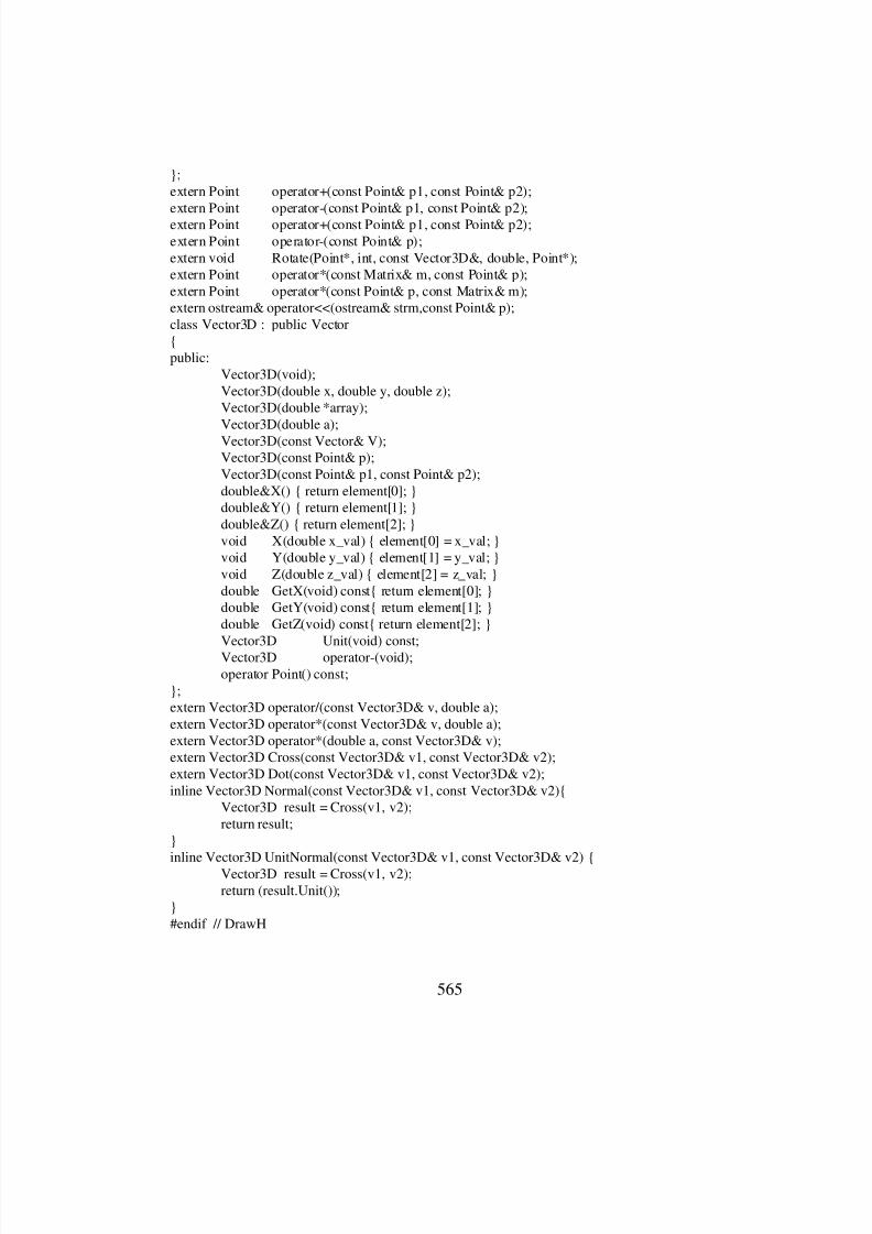
8/3/2019 Chetan Kapoor Dissertation
http://slidepdf.com/reader/full/chetan-kapoor-dissertation 586/612
565
};extern Point operator+(const Point& p1, const Point& p2);extern Point operator-(const Point& p1, const Point& p2);extern Point operator+(const Point& p1, const Point& p2);extern Point operator-(const Point& p);extern void Rotate(Point*, int, const Vector3D&, double, Point*);extern Point operator*(const Matrix& m, const Point& p);extern Point operator*(const Point& p, const Matrix& m);extern ostream& operator<<(ostream& strm,const Point& p);class Vector3D : public Vector{public:
Vector3D(void);Vector3D(double x, double y, double z);Vector3D(double *array);Vector3D(double a);Vector3D(const Vector& V);Vector3D(const Point& p);Vector3D(const Point& p1, const Point& p2);double&X() { return element[0]; }double&Y() { return element[1]; }double&Z() { return element[2]; }void X(double x_val) { element[0] = x_val; }void Y(double y_val) { element[1] = y_val; }void Z(double z_val) { element[2] = z_val; }double GetX(void) const{ return element[0]; }double GetY(void) const{ return element[1]; }double GetZ(void) const{ return element[2]; }Vector3D Unit(void) const;Vector3D operator-(void);operator Point() const;
};extern Vector3D operator/(const Vector3D& v, double a);extern Vector3D operator*(const Vector3D& v, double a);extern Vector3D operator*(double a, const Vector3D& v);extern Vector3D Cross(const Vector3D& v1, const Vector3D& v2);extern Vector3D Dot(const Vector3D& v1, const Vector3D& v2);inline Vector3D Normal(const Vector3D& v1, const Vector3D& v2){
Vector3D result = Cross(v1, v2);return result;
}inline Vector3D UnitNormal(const Vector3D& v1, const Vector3D& v2) {
Vector3D result = Cross(v1, v2);return (result.Unit());
}#endif // DrawH

8/3/2019 Chetan Kapoor Dissertation
http://slidepdf.com/reader/full/chetan-kapoor-dissertation 587/612
566
D.5.3. Shape.h - Polygon and Derivations of the Shape class
/********************************************************************* FILE: Shape.h ** AUTHOR: Chetan Kapoor ** DATE: 21/9/94 ** REVISIONS: ** PURPOSE: This file declares the Shape class ** NOTES: *********************************************************************/ #ifndef ShapeH#define ShapeH#include "Rmath.h"#include "Draw.h"
class Polygon; // forward declaration
typedef Polygon* PolygonP;
enum SHADING { OUTSIDE, INSIDE, BOTHSIDE };enum RENDER { WIREFRAME, SMOOTH, FACETED};
class Attributes{protected:
SHADING current_shading;RENDER current_rendering;
public: Attributes(RENDER render = SMOOTH, SHADING shading = OUTSIDE);Attributes(const Attributes& attr);int SetShading(SHADING);int SetRendering(RENDER);SHADING GetShading(void);RENDER GetRendering(void);Attributes& operator=(const Attributes& attr);
};
class Polygon{protected:
int number_points;Attributes attr;Point *point_array;Vector3D normal;
public:Polygon(Point*, int);Polygon(const Polygon&);
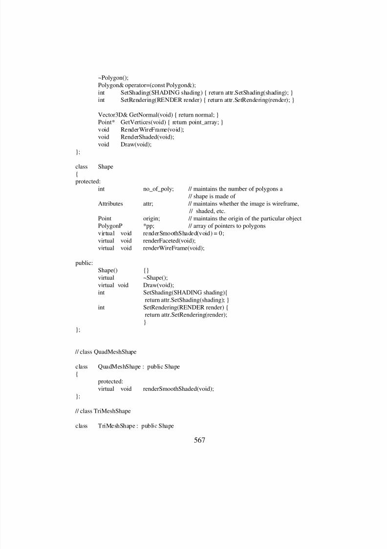
8/3/2019 Chetan Kapoor Dissertation
http://slidepdf.com/reader/full/chetan-kapoor-dissertation 588/612
567
~Polygon();Polygon& operator=(const Polygon&);int SetShading(SHADING shading) { return attr.SetShading(shading); }int SetRendering(RENDER render) { return attr.SetRendering(render); }
Vector3D& GetNormal(void) { return normal; }Point* GetVertices(void) { return point_array; }void RenderWireFrame(void);void RenderShaded(void);void Draw(void);
};
class Shape{protected:
int no_of_poly; // maintains the number of polygons a // shape is made of
Attributes attr; // maintains whether the image is wireframe, // shaded, etc.
Point origin; // maintains the origin of the particular objectPolygonP *pp; // array of pointers to polygonsvirtual void renderSmoothShaded(void) = 0;virtual void renderFaceted(void);virtual void renderWireFrame(void);
public:Shape() {}virtual ~Shape();virtual void Draw(void);int SetShading(SHADING shading){
return attr.SetShading(shading); }int SetRendering(RENDER render) {
return attr.SetRendering(render);}
};
// class QuadMeshShape
class QuadMeshShape : public Shape{
protected:virtual void renderSmoothShaded(void);
};
// class TriMeshShape
class TriMeshShape : public Shape
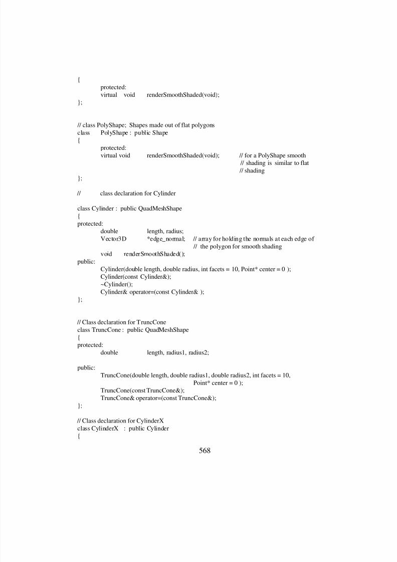
8/3/2019 Chetan Kapoor Dissertation
http://slidepdf.com/reader/full/chetan-kapoor-dissertation 589/612
568
{protected:virtual void renderSmoothShaded(void);
};
// class PolyShape; Shapes made out of flat polygonsclass PolyShape : public Shape{
protected:virtual void renderSmoothShaded(void); // for a PolyShape smooth
// shading is similar to flat // shading
};
// class declaration for Cylinder
class Cylinder : public QuadMeshShape{protected:
double length, radius;Vector3D *edge_normal; // array for holding the normals at each edge of
// the polygon for smooth shadingvoid renderSmoothShaded();
public:Cylinder(double length, double radius, int facets = 10, Point* center = 0 );Cylinder(const Cylinder&);~Cylinder();Cylinder& operator=(const Cylinder& );
};
// Class declaration for TruncConeclass TruncCone : public QuadMeshShape{protected:
double length, radius1, radius2;
public:TruncCone(double length, double radius1, double radius2, int facets = 10,
Point* center = 0 );TruncCone(const TruncCone&);TruncCone& operator=(const TruncCone&);
};
// Class declaration for CylinderXclass CylinderX : public Cylinder{
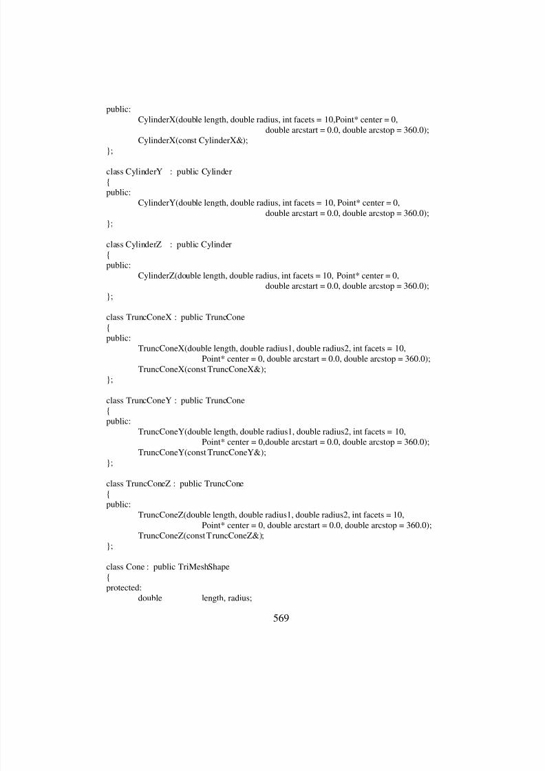
8/3/2019 Chetan Kapoor Dissertation
http://slidepdf.com/reader/full/chetan-kapoor-dissertation 590/612
569
public:CylinderX(double length, double radius, int facets = 10,Point* center = 0,
double arcstart = 0.0, double arcstop = 360.0);CylinderX(const CylinderX&);
};
class CylinderY : public Cylinder{public:
CylinderY(double length, double radius, int facets = 10, Point* center = 0,double arcstart = 0.0, double arcstop = 360.0);
};
class CylinderZ : public Cylinder{public:
CylinderZ(double length, double radius, int facets = 10, Point* center = 0,double arcstart = 0.0, double arcstop = 360.0);
};
class TruncConeX : public TruncCone{public:
TruncConeX(double length, double radius1, double radius2, int facets = 10,Point* center = 0, double arcstart = 0.0, double arcstop = 360.0);
TruncConeX(const TruncConeX&);};
class TruncConeY : public TruncCone{public:
TruncConeY(double length, double radius1, double radius2, int facets = 10,Point* center = 0,double arcstart = 0.0, double arcstop = 360.0);
TruncConeY(const TruncConeY&);};
class TruncConeZ : public TruncCone{public:
TruncConeZ(double length, double radius1, double radius2, int facets = 10,Point* center = 0, double arcstart = 0.0, double arcstop = 360.0);
TruncConeZ(const TruncConeZ&);};
class Cone : public TriMeshShape{protected:
double length, radius;
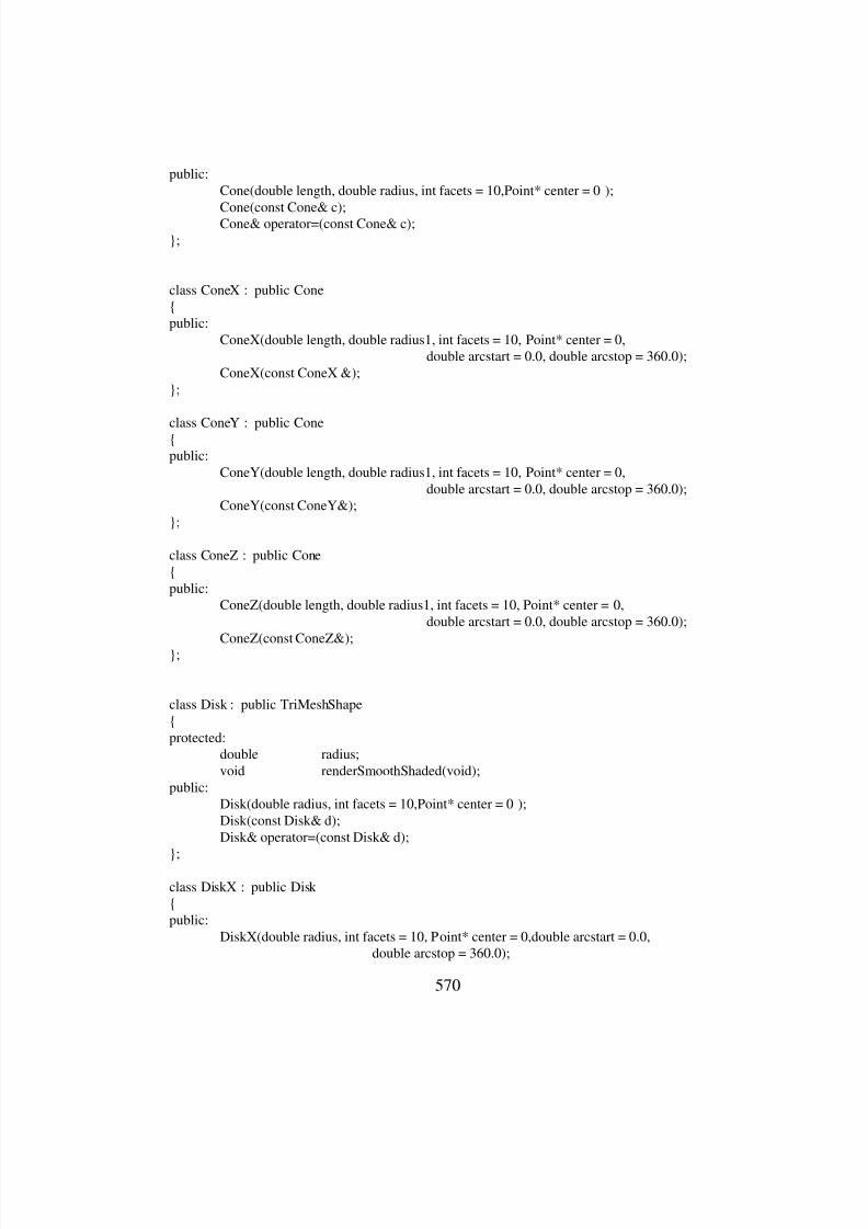
8/3/2019 Chetan Kapoor Dissertation
http://slidepdf.com/reader/full/chetan-kapoor-dissertation 591/612
570
public:Cone(double length, double radius, int facets = 10,Point* center = 0 );Cone(const Cone& c);Cone& operator=(const Cone& c);
};
class ConeX : public Cone{public:
ConeX(double length, double radius1, int facets = 10, Point* center = 0,double arcstart = 0.0, double arcstop = 360.0);
ConeX(const ConeX &);};
class ConeY : public Cone{public:
ConeY(double length, double radius1, int facets = 10, Point* center = 0,double arcstart = 0.0, double arcstop = 360.0);
ConeY(const ConeY&);};
class ConeZ : public Cone{public:
ConeZ(double length, double radius1, int facets = 10, Point* center = 0,double arcstart = 0.0, double arcstop = 360.0);
ConeZ(const ConeZ&);};
class Disk : public TriMeshShape{protected:
double radius;void renderSmoothShaded(void);
public:Disk(double radius, int facets = 10,Point* center = 0 );Disk(const Disk& d);Disk& operator=(const Disk& d);
};
class DiskX : public Disk {public:
DiskX(double radius, int facets = 10, Point* center = 0,double arcstart = 0.0,double arcstop = 360.0);
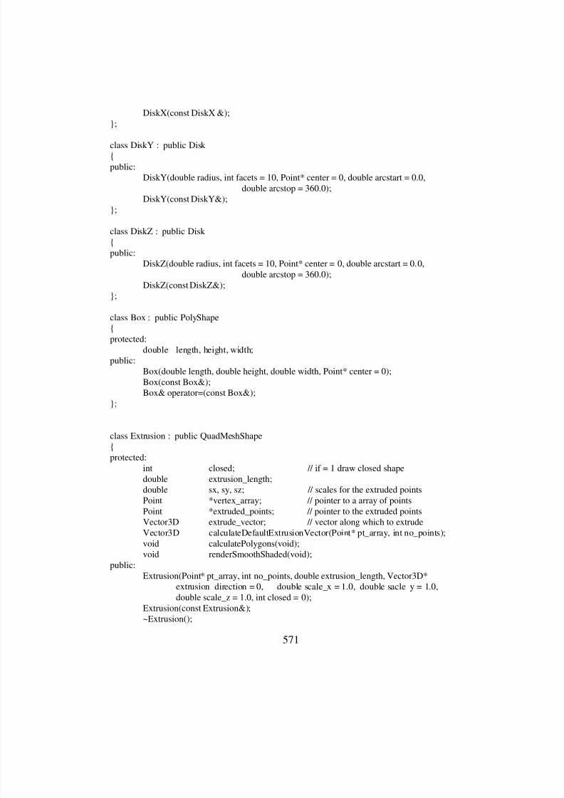
8/3/2019 Chetan Kapoor Dissertation
http://slidepdf.com/reader/full/chetan-kapoor-dissertation 592/612
571
DiskX(const DiskX &);};
class DiskY : public Disk {public:
DiskY(double radius, int facets = 10, Point* center = 0, double arcstart = 0.0,double arcstop = 360.0);
DiskY(const DiskY&);};
class DiskZ : public Disk {public:
DiskZ(double radius, int facets = 10, Point* center = 0, double arcstart = 0.0,double arcstop = 360.0);
DiskZ(const DiskZ&);};
class Box : public PolyShape{protected:
double length, height, width;public:
Box(double length, double height, double width, Point* center = 0);Box(const Box&);Box& operator=(const Box&);
};
class Extrusion : public QuadMeshShape{protected:
int closed; // if = 1 draw closed shapedouble extrusion_length;double sx, sy, sz; // scales for the extruded pointsPoint *vertex_array; // pointer to a array of pointsPoint *extruded_points; // pointer to the extruded pointsVector3D extrude_vector; // vector along which to extrudeVector3D calculateDefaultExtrusionVector(Point* pt_array, int no_points);void calculatePolygons(void);void renderSmoothShaded(void);
public:Extrusion(Point* pt_array, int no_points, double extrusion_length, Vector3D*
extrusion_direction = 0, double scale_x = 1.0, double sacle_y = 1.0,double scale_z = 1.0, int closed = 0);
Extrusion(const Extrusion&);~Extrusion();
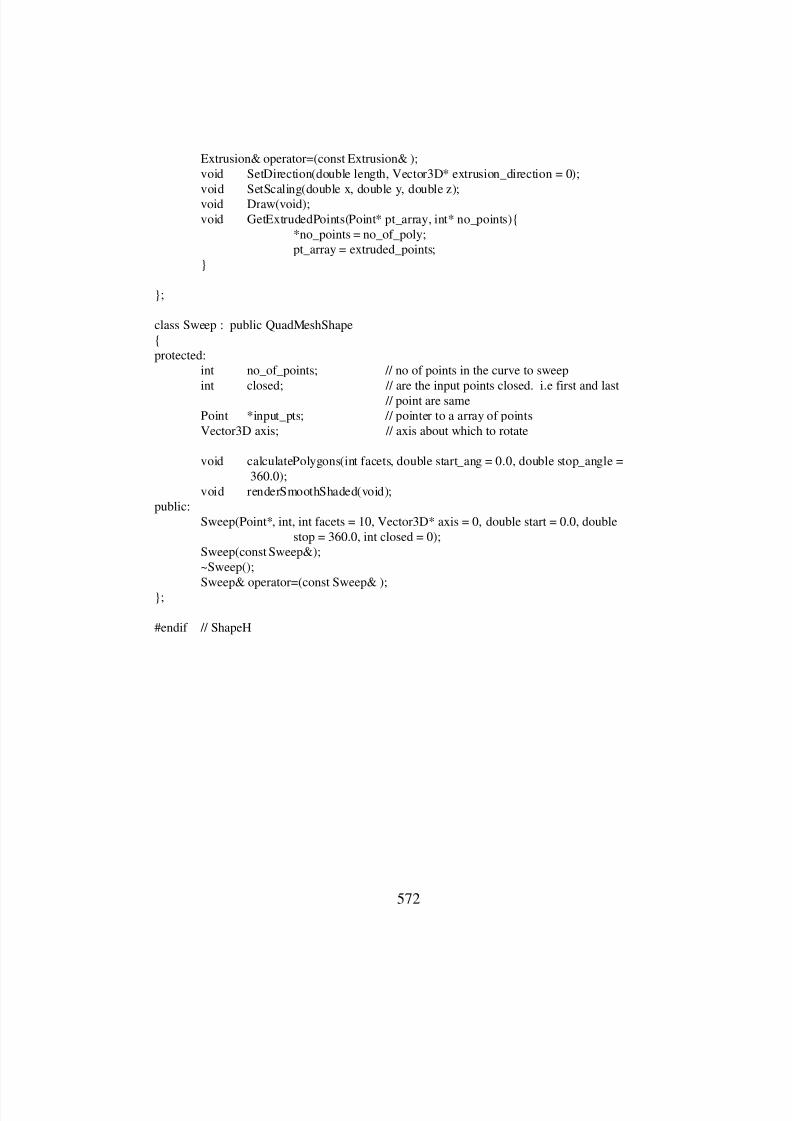
8/3/2019 Chetan Kapoor Dissertation
http://slidepdf.com/reader/full/chetan-kapoor-dissertation 593/612
572
Extrusion& operator=(const Extrusion& );void SetDirection(double length, Vector3D* extrusion_direction = 0);void SetScaling(double x, double y, double z);void Draw(void);void GetExtrudedPoints(Point* pt_array, int* no_points){
*no_points = no_of_poly;pt_array = extruded_points;
}
};
class Sweep : public QuadMeshShape{protected:
int no_of_points; // no of points in the curve to sweepint closed; // are the input points closed. i.e first and last
// point are samePoint *input_pts; // pointer to a array of pointsVector3D axis; // axis about which to rotate
void calculatePolygons(int facets, double start_ang = 0.0, double stop_angle =360.0);
void renderSmoothShaded(void);public:
Sweep(Point*, int, int facets = 10, Vector3D* axis = 0, double start = 0.0, doublestop = 360.0, int closed = 0);
Sweep(const Sweep&);~Sweep();Sweep& operator=(const Sweep& );
};
#endif // ShapeH
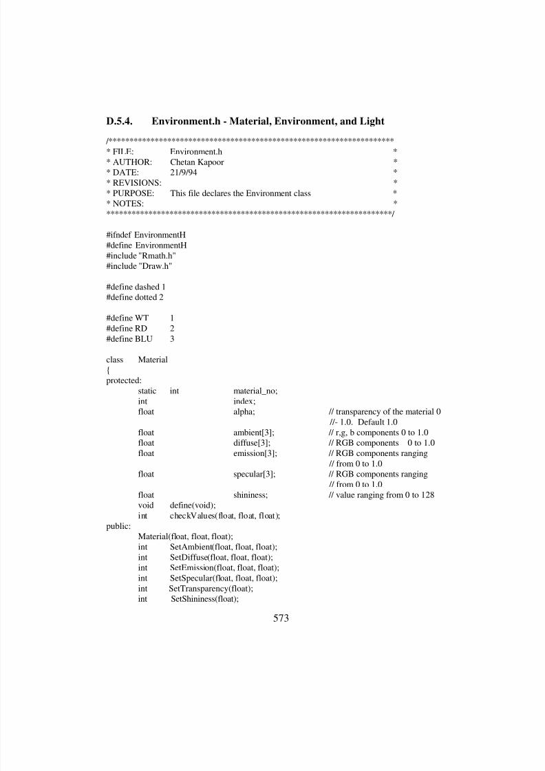
8/3/2019 Chetan Kapoor Dissertation
http://slidepdf.com/reader/full/chetan-kapoor-dissertation 594/612
573
D.5.4. Environment.h - Material, Environment, and Light
/********************************************************************* FILE: Environment.h ** AUTHOR: Chetan Kapoor ** DATE: 21/9/94 ** REVISIONS: ** PURPOSE: This file declares the Environment class ** NOTES: *********************************************************************/
#ifndef EnvironmentH#define EnvironmentH#include "Rmath.h"
#include "Draw.h"
#define dashed 1#define dotted 2
#define WT 1#define RD 2#define BLU 3
class Material{protected:
static int material_no;
int index;float alpha; // transparency of the material 0 //- 1.0. Default 1.0
float ambient[3]; // r,g, b components 0 to 1.0float diffuse[3]; // RGB components 0 to 1.0float emission[3]; // RGB components ranging
// from 0 to 1.0float specular[3]; // RGB components ranging
// from 0 to 1.0float shininess; // value ranging from 0 to 128void define(void);int checkValues(float, float, float);
public:
Material(float, float, float);int SetAmbient(float, float, float);int SetDiffuse(float, float, float);int SetEmission(float, float, float);int SetSpecular(float, float, float);int SetTransparency(float);int SetShininess(float);
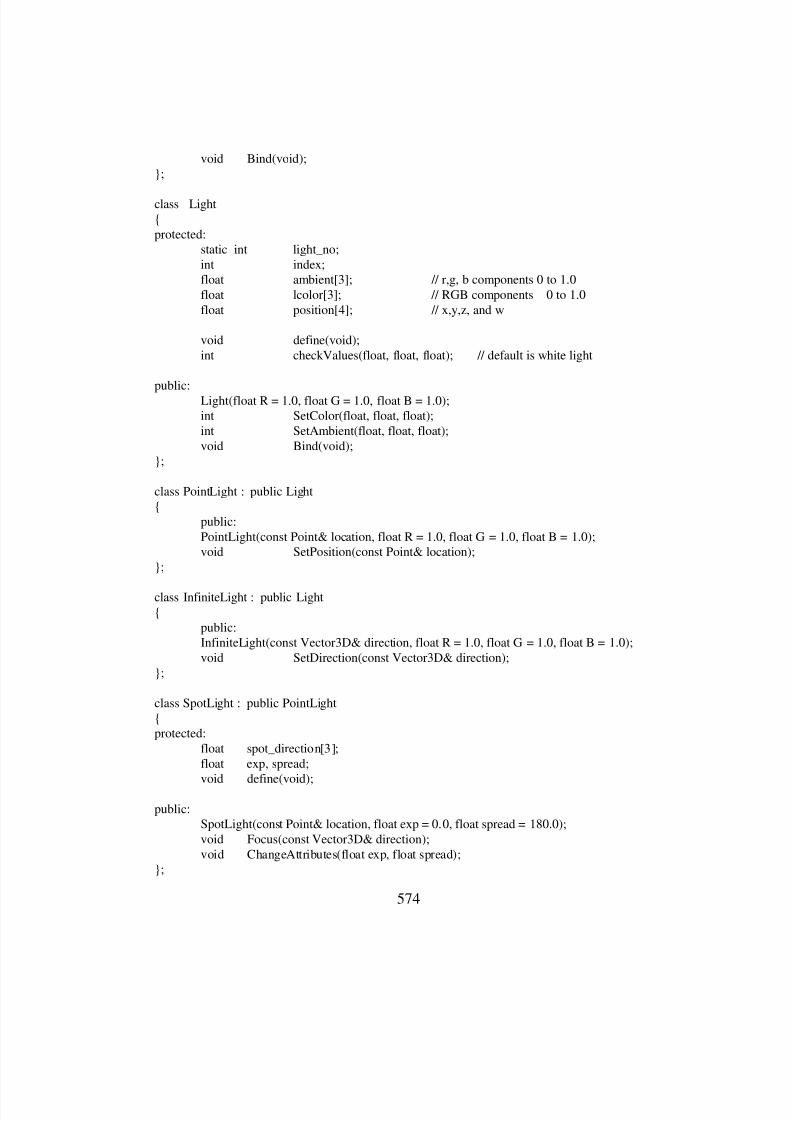
8/3/2019 Chetan Kapoor Dissertation
http://slidepdf.com/reader/full/chetan-kapoor-dissertation 595/612
574
void Bind(void);};
class Light{protected:
static int light_no;int index;float ambient[3]; // r,g, b components 0 to 1.0float lcolor[3]; // RGB components 0 to 1.0float position[4]; // x,y,z, and w
void define(void);int checkValues(float, float, float); // default is white light
public:Light(float R = 1.0, float G = 1.0, float B = 1.0);int SetColor(float, float, float);int SetAmbient(float, float, float);void Bind(void);
};
class PointLight : public Light{
public:PointLight(const Point& location, float R = 1.0, float G = 1.0, float B = 1.0);void SetPosition(const Point& location);
};
class InfiniteLight : public Light{
public:InfiniteLight(const Vector3D& direction, float R = 1.0, float G = 1.0, float B = 1.0);void SetDirection(const Vector3D& direction);
};
class SpotLight : public PointLight{protected:
float spot_direction[3];float exp, spread;void define(void);
public:SpotLight(const Point& location, float exp = 0.0, float spread = 180.0);void Focus(const Vector3D& direction);void ChangeAttributes(float exp, float spread);
};

8/3/2019 Chetan Kapoor Dissertation
http://slidepdf.com/reader/full/chetan-kapoor-dissertation 596/612
575
// class declaration of Environmentclass Window;typedef Window* WindowP;class Environment{protected:
static int win_no;WindowP window_array[10]; // max of 10 windowsWindowP active_window;void generateMaterialDefinitions(void);void destroyMaterialDefinitions(void);void initializeViewing(void);void initializeDevices(void);
public:Environment(void);~Environment(void);WindowP CreateWindow(char*name , long size_x = 0, long size_y = 0);WindowP CreateWindow(char* name, long x1, long y1, long x2, long y2);void SetActiveWindow(WindowP win);void SetActiveWindow(long window_id);void SceneRotation(int* device, int no_device, void (*func)(void) );void SceneTranslation(int* device, int no_device, void (*func)(void) );void SceneZooming(int* device, int no_device, void (*func)(void) );void DrawScene(void (*func)(void));
};
class Window{
protected:long window_id;char w_name[32];float background[3];float view_ptx, view_pty, view_ptz;float view_sightx, view_sighty, view_sightz;float scene_rotx, scene_roty, scene_rotz; // rotations of the scenefloat trans_x, trans_y, trans_z; // translations of the scenefloat zoom_factor; // zoom-factor for the scenevoid initialize(void);
public:Window(char* name, long size_x = 0, long size_y = 0);Window(char* name, long x1, long y1, long x2, long y2);long GetWindowID(void) const { return window_id; }void Move(long orgx, long orgy);

8/3/2019 Chetan Kapoor Dissertation
http://slidepdf.com/reader/full/chetan-kapoor-dissertation 597/612
576
void MoveRelative(long distx, long disty);void ResizeAndReposition(long x1, long y1, long x2, long y2);void SetMinSize(long x, long y);void SetMaxSize(long x, long y);void SetAspectRatio(long x, long y);void SetBackground(float* color);void SetViewSight(float x, float y, float z){
view_sightx = x; view_sighty = y; view_sightz = z;}void SetViewPoint(float x, float y, float z){
view_ptx = x; view_pty = y; view_ptz = z;}void SetSceneRotation(float x, float y, float z){
scene_rotx = x; scene_roty = y; scene_rotz = z;}void SetSceneTranslation(float x, float y, float z){
trans_x = x; trans_y = y; trans_z = z;}void SetZoomFactor(float z){
zoom_factor = z;}float* GetBackground(void) {
return background;}void GetViewSight(float& x, float& y, float& z) const {
x = view_sightx; y = view_sighty; z = view_sightz;}void GetViewPoint(float& x, float& y, float& z) const {
x = view_ptx; y = view_pty; z = view_ptz;}void GetSceneRotation(float& x, float& y, float& z) const {
x = scene_rotx; y = scene_roty; z = scene_rotz;}
void GetSceneTranslation(float& x, float& y, float& z) const {x = trans_x; y = trans_y; z = trans_z;
}void GetZoomFactor(float& z) const {
z = zoom_factor;}
};
#endif // EnvironmentH

8/3/2019 Chetan Kapoor Dissertation
http://slidepdf.com/reader/full/chetan-kapoor-dissertation 598/612
577
D.5.5. Defines.h: Material and Color Declarations
/********************************************************************* FILE: Defines.h ** AUTHOR: Chetan Kapoor ** DATE: 21/9/94 ** REVISIONS: ** PURPOSE: This file contains some global material and color defs. ** All ’.c’ files which plan to use these material and color ** definitions should include this file ** NOTES: *********************************************************************/ #ifndef DefineH#define DefineH
class Material;
extern float yellow[3], blue[3];extern float ltblue[3], black[3];extern float white[3], red[3];extern float ltred[3], green[3];extern float ltgreen[3], gray[3], background[3];
extern Material *brightred, *darkred, *lightred;extern Material *brightgreen, *darkgreen, *lightgreen;extern Material *dullyellow, *creme, *lightcreme;extern Material *brightblue, *darkblue, *medlightblue, *lightblue;
extern Material *gray1, *gray2, *brushedalum, *polishedalum;extern Material *gray3, *flatblack, *lightbrown, *darkbrown;extern Material *flatwhite, *specularwhite, *specularblack;
#endif // DefineH

8/3/2019 Chetan Kapoor Dissertation
http://slidepdf.com/reader/full/chetan-kapoor-dissertation 599/612
578
References
Aalund, M.P., “Design and Development of a Multi-Channel Robotic Controller,”
Master’s Thesis, Department of Mechanical Engineering, Univ. of Texas at
Austin, TX (1991).
Aalund, M.P., Geisinger, J.W., Puls, R.C., and Tesar, D. “Development of a
Digital Intelligent Servo Controller for Modular Robots,” Proceedings of the
Third International Symposium on Measurement and Control in Robotics,
AMMA-Via Vela 17-Torino, Italy, Sept., 1993, pp. Bm. I-31 to Bm. I-36.
ABB Robotics Incorporated, Operating/Teach Manual for Cincinnati Milacron T 3
600/700/800 series, Version 5.0, Release 5.0.
Aken, L.V., and Brussel, H.V., “Robot Programming Languages: The Statement
of a Problem,” Robotica, Vol. 6, 1988, pp. 141-148.
Alander, J.T., Frisk, M., Tuominen, J., and Vuolteenaho, M., “An Outline of a
Modular and Multiarm Assembly Cell with Object-Oriented Control,”
Proceedings IEEE International Conference on Robotics and Automation,
1990, pp. 592-597.
Ambrose, C., “The Development of an Interactive Synthesis Tool for IntelligentControllers of Modular, Reconfigurable Robots,” Ph.D. Dissertation, Dept. of
Mechanical Engineering, University of Texas at Austin, Austin, TX
(December, 1992).
Anderson, J.N., and Smiarowski, A., “A Fast Computer Architecture for the
Control of Robots,” Computers in Electrical Engineering, Vol. 17, No. 3,
1991, pp. 217-235.
Anderson, R.J., “SMART: A Modular Architecture for Robots and
Teleoperation,” Proceedings of the IEEE Conference on Robotics and
Automation, May, 1993, Atlanta, Georgia.
Banachiewicz, M., “SEL: Robotic Sensor/Effector Programming Language,”
Proc. IEEE International Conference on Robotics and Automation, Vol. 3,
1986, pp. 1779-1784.
8/3/2019 Chetan Kapoor Dissertation
http://slidepdf.com/reader/full/chetan-kapoor-dissertation 600/612
579
Baugh, J.W.Jr., and Rehak, D.R., "Data Abstraction in Engineering Software
Development," Journal of Computing in Civil Engineering, Vol. 6, No. 3,July 1992, pp. 282-301.
Benedict, C.E., and Tesar, D., “Model Formulation of Complex Mechanisms with
Multiple Inputs: Part1-Geometry,” ASME Journal of Mechanical Design,
Vol. 100, 1979, pp. 747-719.
Bihari, T.E., and Gopinath, P., "Object-Oriented Real-Time Systems: Concepts
and Examples," IEEE Computer , December, 1992, pp. 25-32.
Birmingham, W.P., and Gupta, A.P., “The MICON System for Computer
Design,” University Libraries, Carnegie Mellon University, Pittsburgh,
Pennsylvania, 1988.
Bison, P., and Gini, M., “An Object-Oriented Approach to Robot Programming,”
Computer Integrated Manufacturing Systems, Vol. 2, No. 1, February 1989,
pp. 29-34.
Bit3 Computer Corporation, Multibus I-VME Adapter Model 422, User’s Guide.
Blume, C., and Jakob, W., “Design of a Structured Robot Language,” Advanced
Software in Robotics, 1984, pp. 127-143.
Bolinger, D., and Bronson, T., Applying RCS and SCCS. O’Reilly and
Associates, Inc., 1995.Bonner, S., and Shin, K.G., "A Comparative Study of Robot Languages," IEEE
Computer , Vol. 15, No. 12, 1982, pp. 82-96.
Booch, G., Object Oriented Analysis and Design with Applications. Second
Edition, Redwood City, CA: The Benjamin/Cummings Publishing
Company, Inc., 1994.
Boyer, M., Daneshmend, L.K., Hayward, V., and Foisy, A., "An Object-Oriented
Paradigm for the Design and Implementation of Robot Planning and
Programming Systems," Proc. IEEE Int. Conf. on Robotics and Automation,
April 1991, pp. 204-209.
Brain, M., Win32 System Services: The Heart of Windows NT . PTR Prentice
Hall, Englewood Cliffs, New Jersey, 1994.
8/3/2019 Chetan Kapoor Dissertation
http://slidepdf.com/reader/full/chetan-kapoor-dissertation 601/612
580
Browning, G.T., “The Physical Significance of Kinematic and Dynamic
Performance Criteria for Serial Redundant Manipulators,” Masters Thesis,Dept. of Mechanical Engineering, University of Texas at Austin, TX (1996).
Bullock, D.M., and Oppenheim, I.J., "Object-Oriented Programming in Robotics
Research for Excavation," Journal of Computing in Civil Engineering, Vol.
6, No. 3, July 1992, pp. 370-385.
Burchard, R.L., and Feddema, J.T., “Generic Robotic and Motion Control API
Based on GISC-Kit Technology and CORBA Communications,”
Proceedings IEEE International Conference on Robotics and Automation,
April 1996, pp. 712-717.
Butler, M., and Tesar, D., "A Generalized Modular Architecture for Robot
Structures," Manufacturing Review , Vol. 2, No. 2, June 1989, pp. 91-118.
Butner, S., Wang, Y., Mangaser, A., and Jordan, S., “Design and Simulation of
RIPS: An Advanced Robot Control System,” Proceedings IEEE
International Conference on Robotics and Automation, Vol. 1, 1988, pp.
470-474.
Champeaux, D., Lea, D., and Faure, P., “The Process of Object-Oriented Design,”
Conference on Object-Oriented Programming Systems, Languages,
Applications, 1992, pp. 45-62.Chen, C., Trivedi, M.M., and Bidlack, C.R., “Simulation and Graphical Interface
for Programming and Visualization of Sensor-Based Robot Operation,”
Proceedings IEEE International Conference on Robotics and Automation,
May 1992, pp. 1095-1101.
Cheng, H. H., “Extending C and FORTRAN for Design Automation,” ASME
Transactions, Journal of Mechanical Design, Vol. 117, No. 3, Sept. 1995,
pp. 390-395.
Cimetrix Incorporated, “CX3000 Open Architecture Controller,” Product
Description, 1996.
Cleary, K., and Tesar, D., “Incorporating Multiple Criteria in the Operation of
Redundant Manipulators,” Proceedings IEEE International Conference on
Robotics and Automation, Vol. 1, 1990, pp. 618-623.
8/3/2019 Chetan Kapoor Dissertation
http://slidepdf.com/reader/full/chetan-kapoor-dissertation 602/612
581
Coad, P. and Yourdon, E., Object-Oriented Analysis. Prentice-Hall, Englewood
Cliffs, NJ, 1990.Coplien, J. O., Advanced C++: Programming Styles and Idioms. Addison-
Wesley Publishing Company, 1994, pp.520.
Cox, I.J., "C++ Language Support for Guaranteed Initialization, Safe Termination
and Error Recovery in Robotics," IEEE Council on Robotics and Automation,
1988, pp. 641-643.
Cox, I.J., and Gehani, N.H., "Concurrent C and Robotics, "Proc. IEEE Int. Conf.
on Robotics and Automation, 1987, pp. 1463-1468.
Cox, I.J., Kapilow, D.A., and Kropfl, W.J., “Real-Time Software for Robotics,”
AT&T Technical Journal, Vol. 67, No. 2, March-April 1988, pp. 61-72.
Craig, J.J., Introduction to Robotics Mechanics and Controls. 1986, Addision-
Wesley.
Cybernet Systems Corporation, Implementation of a Compact 6 Degree of
Freedom Force Reflecting Hand Controller with Cueing Modes.
Duffy, J., Analysis of Mechanisms and Robot Manipulators, Wiley, New-York,
1980.
Duhaut, D., Bidaud, P., and Fontaine, D., “Iada: A Language for Robot
Programming Based on Ada,” Robotics and Autonomous Systems, Vol. 9,1992, pp. 299-304.
Force Computers Incorporated, Force CPU-30 User’s Manual, Revision 2.
Fresonke, D.A., Hernandez, E., and Tesar, D., “Deflection Prediction for Serial
Manipulators,” Proceedings IEEE Conference on Robotics and Automation,
April 24-29, 1988, pp. 482-487.
Geppert, L., “Solid State,” IEEE Spectrum, January 1995, pp. 35-39.
Giddings, R.A., “Development and Demonstration of General, Real-Time Control
Software for Robotic Manipulators,” Master’s Thesis, Dept. of Mech. Eng.,
Univ. of Texas, Austin, TX (1992).
Grossman, D., “AML as a Plant Floor Language,” Robotics and Computer
Integrated Manufacturing, Vol. 2, No. 3/4, 1986, pp. 215-217.
8/3/2019 Chetan Kapoor Dissertation
http://slidepdf.com/reader/full/chetan-kapoor-dissertation 603/612
582
Grupinski, S., “Design of a System of Modular Robotic Actuators,” Master’s
Thesis, Department of Mechanical Engineering, Univ. of Texas at Austin, TX(1996).
Gruver, W.A., Soroka, B.I., Craig, J.J., and Turner, T.L., "Evaluation of
Commercially Available Robot Programming Languages, Tech. Pap. Soc.
Manuf. Eng., 1983, pp. 58-68.
Harima, T., and West, H., “Natural Robot Programming System,” Proceedings
IEEE/RSJ International Conference on Intelligent Robots and Systems, 1992,
pp. 750-756.
Hayward, V., and Paul, R.P., “Robot Manipulator Control Under UNIX RCCL:
A Robot Control “C” Library,” The International Journal of Robotics
Research, Vol. 5, No. 4, 1986, pp. 94-111.
Henderson-Sellers, B., and Edwards, J.M., “The Object-Oriented Systems Life
Cycle,” Communications of the ACM , September 1990, Vol. 33, No. 9, pp.
142-159.
Hernandez, E., Sreedhar, R. and Tesar, D., “Computational Requirements for the
Design and Control of the Fifth Generation Robot,” Robotics Research
Group, The University of Texas at Austin, 1989.
Hicks, C., Fundamental Concepts in the Design of Experiments. Springer-Verlag,Berlin, 1967.
Hill, B. M., and Tesar, D. "Rapid Analysis Manipulator Program (RAMP) as a
Design Tool for Serial Revolute Robots", Proceedings of the 1996 IEEE
International Conference on Robotics and Automation.
Hooper, R.N., “Multicriteria Inverse Kinematics for General Serial Robots,”
Ph.D. Dissertation, Dept. of Mechanical Engineering, University of Texas at
Austin, TX (1994).
Hooper, R.N., “The Interactive Assembly and Computer Animation of
Reconfigurable Robotic Systems,” Master’s Thesis, Dept. of Mechanical
Engineering, Univ. of Texas, Austin, TX (1990).
Horowitz, E., Sahni, S., and Anderson-Freed, S., Fundamentals of Data
Structures in C . Computer Science Press, 1993.
8/3/2019 Chetan Kapoor Dissertation
http://slidepdf.com/reader/full/chetan-kapoor-dissertation 604/612
583
Hudgens, J.C., “Static Robot Compliance and Metrology Procedures with
Application to a Light Machining Robot,” Ph.D. Dissertation, Dept. of Mechanical Engineering, Univ. of Texas, Austin, TX (1992).
Hutchinson, S.A., and Kak, A.C., “Fprolog: A language to integrate Logic and
Functional Programming for Automated Assembly,” Proceedings IEEE
International Conference on Robotics and Automation, Vol. 2, 1986, pp.
904-909.
Iaconics, J.M., “Design and Prototype Development of Robot Actuator Modules,”
Masters Thesis, Dept. of Mechanical Engineering, University of Texas at
Austin, TX (1991).
Isherwood, D., “DOS and Real-Time,” Third International Conference on
Software Engineering for Real-Time Systems, 1991, pp. 156-163.
Izaguirre, A., Hashimoto, M., Paul, R.P., and Hayward, V., “A New
Computational Structure for Real-Time Dynamics,” The International
Journal of Robotics Research, Vol. 11, No. 4, August 1992, pp. 346-361.
Jordan, D., “Implementation Benefits of C++ Language Mechanisms,”
Communications of the ACM , September 1990, Vol. 33, No. 9, pp. 61-64.
Kapoor, C., “Off-line Programming of a Robot Manipulator Using Graphical
Simulation,” Master’s Thesis, The University of Alabama, Tuscaloosa, AL(1992).
Kapoor, C., “Source Code Development and Formatting Guidelines,” Internal
Document, Robotics Research Group, The University of Texas at Austin,
1995.
Karlen, J.P., Thompson, J.M., Vold, H.I., Farrel, J.D., and Eismann, P.H., “A
Dual-Arm Dexterous Manipulator System with Anthropomorphic
Kinematics,” Proceedings IEEE Conference on Robotics and Automation,
1990, pp. 368-373.
Khosla, P. and Kanade, T., “Real-Time Implementation and Evaluation of Model-
Based Controls on CMU DD ARM II,” Proc. IEEE Conf. on Robotics and
Automation, 1986, pp. 1546-1555.

8/3/2019 Chetan Kapoor Dissertation
http://slidepdf.com/reader/full/chetan-kapoor-dissertation 605/612
584
Knopf, C.A., “A Roadmap For Modular Robot Metrology,” Master’s Thesis,
Department of Mechanical Engineering, Univ. of Texas at Austin, TX(1994).
Korson, T., and McGregor, J.D., “Understanding Object-Oriented: A Unifying
Paradigm,” Communications of the ACM , September 1990, Vol. 33, No. 9,
pp. 40-60.
LaLonde, W.R., Thomas, D.A., and Johnson, K., "Smalltalk as a Programming
Language for Robotics," Proc. IEEE Int. Conf. on Robotics and Automation,
1987, pp. 1456-1462 .
Landman, R.G., “Selecting a Real-Time Operating System,” Embedded Systems
Programming, Volume 9, Number 4, April 1996, pp. 79-95.
Leu, M.C., "Robotics Software Systems," Robotics and Computer-Integrated
Manufacturing, Vol. 2, No. 1, 1985, pp. 1-12.
Lewis, T., “Where is Computing Headed?” IEEE Computer , August 1994.
Lippman, S., C++ Primer. 2nd Edition, Addision Wesely.
Lozano-Peréz, "Robot Programming," Proceedings of the IEEE , Vol. 71, No. 7,
July 1983, pp. 821-841.
Marrs, M., “Design of an Advanced, High-Precision, Seven Degree-of-Freedom
Modular Robotic Manipulator,” Master’s Thesis, Dept. of MechanicalEngineering, Univ. of Texas, Austin, TX (1996).
Mellor, S., Hecht, A., Tryon, D., and Hywari, W. “Object-Oriented Analysis:
Theory and Practice,” Course Notes, in Object-Orieneted Programming
Systems, Languages, and Applications. San Diego, CA: OOPSLA’88,
September 1988, pp. 1-3.
Miller, D.J., and Lennox, R.C., "An Object-Oriented Environment for Robot
System Architectures," IEEE Control Systems, February 1991, pp. 14-23.
Mohri, S., Takeda, K., Hata, Matsuzaki, S.J.K., and Hyodo, Y., “Robot Language
From the Standpoint of FA System Development - An Outline of FA-
BASIC,” Robotics and Computer Integrated Manufacturing, Vol. 2, No. 3/4,
1985, pp. 279-292.
8/3/2019 Chetan Kapoor Dissertation
http://slidepdf.com/reader/full/chetan-kapoor-dissertation 606/612
585
Nakamura, Y., Advanced Robotics: Redundancy and Optimization. Addison-
Wesley Publishing Company, 1991, pp. 336.Narasimhan, S., Siegel, D.M., and Hollerbach, J.M., “Condor: A Revised
Architecture for Controlling the Utah-MIT Hand,” Proceedings IEEE
International Conference on Robotics and Automation, Vol. 2, 1988, pp.
446-449.
National Instruments, “Instrumentation Reference and Catalogue,” 1996.
Oram, A., and Talbott, S., Managing Projects with make. O’Reilly and
Associates, Inc., 1995.
Pahl, G. and Beitz, W., Engineering Design: A Systematic Approach. Springer-
Verlag, The Design Council, Berlin, 1988.
Park, W.T., “The SRI Robot Programming System (RPS),” Technical Paper
Society of Mechanical Engineers, pp. 22-41.
Perry, B. R., “The Development of Distance Functions and Their Higher-Order
Properties for Aritifical Potential Field-Based Obstacle Avoidance,” Master’s
Thesis, Department of Mechanical Engineering, Univ. of Texas at Austin, TX
(1995).
Peterson, J, “Criteria-Based Performance Evaluation of Manual Controllers,”
Master’s Thesis, Department of Mechanical Engineering, Univ. of Texas atAustin, TX (1996).
Pimentel, J.R., "An Object Oriented Environment for Intelligent Automation
Systems," Proc. IEEE Int. Conf. on Robotics and Automation, 1990, pp. 723-
728.
Potter, D., “Getting on the Right Bus,” Test and Measurement World, February,
1992, pp. 65-70.
Potter, David, “Getting on the Right Bus,” Test and Measurement World ,
February, 1992,
pp. 65-70.
Press, W.H., Flannery, B.P., Teukolsky, S.A., and Vetterling, W.T., Numerical
Recipes in C The Art of Scientific Computing. Cambridge University Press,
Cambridge, England, 1991.
8/3/2019 Chetan Kapoor Dissertation
http://slidepdf.com/reader/full/chetan-kapoor-dissertation 607/612
586
Puls, R.C., “Internal Communications and Interfaces for Modular Robotics,”
Masters Thesis, Dept. of Mechanical Engineering, University of Texas atAustin, TX (May, 1994).
Rackers, K.J., “Development and Demonstration of a Coordinated Control
System for Dual-Arm Robots,” Master’s Thesis, Department of Mechanical
Engineering, Univ. of Texas at Austin, TX (1996).
Rembold, U., Blume, C., and Frommherz, B.J., “The Proposed Robot Software
Interfaces SRL and IRDATA,” Robotics and Computer Integrated
Manufacturing, Vol. 2, No. 3/4, 1985, pp. 219-225.
Robotics Research Group, “The Development and Demonstration of a Class of
Modular, Dexterous, Medium Capacity Manipulator Structures,” Proposal to
DARPA (1991).
RogueWave Software, C++ Booch Components, C++ Class Library for
Multithreading and Storage Management, Class Catalog, Version 2.3
RogueWave Software, Tools.h++, Foundation Class Library for C++
Programming, Introduction and Reference Manual, Version 6.
Rubin, M.D., “Development of Real-Time Operational Software for Fault-
Tolerance Testbed,” Master’s Thesis, Univ. of Texas, Austin, TX (1993).
Salkind, L., “The SAGE Operating System,” Proceedings IEEE InternationalConference on Robotics and Automation, Vol. 2, 1988, pp. 860-865.
Schmitz, D., Khosla, P., Hoffman, R., and Kanade, T., “CHIMERA: A Real-
Time Programming Environment,” Proceedings IEEE International
Conference on Robotics and Automation, Vol. 2, 1989, pp. 846-852.
Schneider, S.A., Chen, V.W., Pardo-Castellote, G., “Control Shell: A Real-Time
Software Framework,” AIAA Conference on Intelligent Robots in Field,
Factory, Service, and Space, March, 1994.
Shanblatt, M.A., and Leung, S.S., “Computer Architecture Design for Robotics,”
Proceedings IEEE International Conference on Robotics and Automation,
Vol. 1, 1988, pp. 453-456.
Shlaer, S., and Mellor, S.J., Object-Oriented Systems Analysis: Modeling the
World in Data. Yourdon Press Computing Series, 1988, pp. 144.
8/3/2019 Chetan Kapoor Dissertation
http://slidepdf.com/reader/full/chetan-kapoor-dissertation 608/612
587
Silberschatz, and Gahin, Operating Systems Concepts. Fourth Edition, Addision
Wesley, 1994.Smith, M.G., "An Environment for More Easily Programming a Robot," Proc.
IEEE Int. Conf. on Robotics and Automation, May 1992 ,pp. 10-16.
Soroka, B. I., “Designing Languages for Robot Systems,” Technical Paper
Society of Mechanical Engineers, 1984.
Soroka, B.I., “What Can’t Robot Languages Do?,” Technical Paper Society of
Mechanical Engineers, pp. 1-8.
Sreevijayan, D., and Tesar, D., "On the Design of Fault-tolerant Robotic
Manipulator Systems," Proc. of the Third Int. Symposium on Measurement
and Control in Robotics, Turin, Italy, September, 1993.
Stankovic, J.A., “Misconceptions About Real-Time Computing,” Computer ,
October 1988, pp. 10-19.
Stewart, D.B., and Khosla, P.K., “Real-Time Scheduling of Dynamically
Reconfigurable Systems,” IEEE International Conference on Systems
Engineering, Aug 1991, pp. 139-142.
Stewart, D.B., Schmitz, D.E., and Khosla, P., “Implementing Real-Time Robotic
Systems Using CHIMERA II,” Proceedings IEEE International Conference
on Robotics and Automation, 1990, pp. 598-603.Stewart, D.B., Volpe, R.A., and Khosla, P.K., “Integration of Real-Time Software
Modules for Reconfigurable Sensor-Based Control Systems,” Proceedings
IEEE/RSJ International Conference on Intelligent Robots and Systems, July
1992, pp. 325-332.
Strang, G., Linear Algebra and its Applications, Third Edition, Harcourt Bruce
Jovanovich, 1988.
Sturzenbecker, M.C. "Building an Object-Oriented Environment for Distributed
Manufacturing Software," Proc. IEEE International conference on Robotics
and Automation, April 1991, pp. 1972-1978.
Taylor, R.H., Korein, J.U., Maier, G., and Durfee, L.F., “A General-Purpose
Control Architecture for Programmable Automation Research,” Robotics
Research: The Third International Symposium, 1986, pp. 165-173.

8/3/2019 Chetan Kapoor Dissertation
http://slidepdf.com/reader/full/chetan-kapoor-dissertation 609/612
588
Tesar, D., “Intelligent Actuators for Space,” White Paper, Robotics Research
Group, The University of Texas at Austin, TX (1996).Tesar, D., “Integration of Intelligent Machines and Robotics for Automation in
Automotive Plants,” White Paper, Robotics Research Group, The University
of Texas at Austin, TX (1996)
Tesar, D., “Operational Software For Enhanced Reliability and Performance of
Advanced Manufacturing Systems,” Texas ATP Proposal, June 22, 1993.
Tesar, D., “Status of U.S. Manufacturing,” Robotics Research Group, The
University of Texas at Austin, TX (1994).
Tesar, D., “Thirty Year Forecast: The Concept of a Fifth Generation of Robotics-
-The Super Robot,” Manufacturing Review, Vol. 2, No. 1, March 1989, pp.
16-25.
Tesar, D., and Matthew, G.K., The Dynamic Synthesis, Analysis, and Design of
Modeled Cam Systems. Lexington Books, 1976.
Thomas, M., and Tesar, D., “Dynamic Modeling of Serial Manipulator Arms,”
ASME Journal of Dynamic Systems, Measurement and Control, Vol. 104,
No. 3, 1982, pp. 218-228.
Todd, M., and Green, D.G., “An Object-Oriented Approach to Robotic Motion,”
Proceedings of the IEEE Southeastcon, 1993, 8p.Tomiyama, K., Honda, F., Shinoda, H., and Tanaka, J., “A Robot Control System
Based on a UNIX Work-Station,” IEEE International Conference on Systems
Engineering, Aug 1991, pp. 125-128.
Unimation Robotics, 500 Series Equipment and Program Manual, 398P1,
February 1983.
Van Doren, “Criteria Development to Support Decision Making Software for
Modular, Reconfigurable Robotic Manipulators,” Master’s Thesis, Dept. of
Mechanical Engineering, Univ. of Texas, Austin, TX (1992).
Volz, R.A., Mudge, T.N., and Gal, D.A., "Using ADA as a Robot System
Programming Language," Tech. Pap. Soc. Manuf. Eng., 1983, pp. 42-57.
Vuskovic, M.I., Riedel, A.L., and Do, C.Q., “The Robot Shell,” International
Journal of Robotics and Automation, Vol. 3, No. 3, 1988, pp. 165-176.
8/3/2019 Chetan Kapoor Dissertation
http://slidepdf.com/reader/full/chetan-kapoor-dissertation 610/612
589
Wander, J.P., “Development of Robot Deflection Compensation for Improved
Machining Accuracy,” Ph.D. Dissertation, Dept. of Mechanical Engineering,University of Texas at Austin, TX (1992).
Wander, J.P., and Tesar, D., “Pipelined Computation of Manipulator Modeling
Matrices,” IEEE Journal of Robotics and Automation, Vol. RA-3, No. 6,
December 1987.
White, Z., Rational Rose Essentials: Using the Booch Method.
Benjamin/Cummings.
Whitney, D.E., “Resolved Rate Motion Control of Manipulator and Human
Prostheses,” IEEE Transactions on Man-Machine Systems, Vol. MMS-10,
No. 2, pp. 47-53, 1969.
Whitney, D.E., “The Mathematics of Coordinated Control of Prostheses and
manipulators,” Journal of Dynamic Systems, Measurement, and Controls,
94(4), pp. 303-309, 1972.
WindRiver Systems, AT&T Language System Library Manual, Version 3.0.
WindRiver Systems, VxWorks Programmer’s Guide, Version 5.2.
WindRiver Systems, VxWorks Reference Manual, Version 5.2.
WindRiver Systems, Wind Foundation Classes Component Release Supplement ,
1.0 Beta.Yeh, R.T., Software Engineering Report, International Software Systems Inc.,
July 28, 1993.
Yi, B.J., “Analysis of Redundantly Actuated Mechanisms With Applications to
Design and Control of Advanced Robotic Systems,” Ph.D. Dissertation,
Dept. of Mechanical Engineering, Univ. of Texas, Austin, TX (1992).
Young, G.E. and Douglas, E.G., “Real-Time Software Development Concepts for
Engineering Applications,” Proceedings of the Winter Annual Meeting of the
ASME , Nov. 25-30, 1990, pp. 1-7.
Yourdon, E., and Constantine, L.L., Structured Design. Prentice Hall, 1979.
Yuta, S. and Kanayama, Y., “Computer Architecture for Intelligent Robots,”
Journal of Robotic Systems, Vol. 2, No. 3, 1985, pp. 237-251.
8/3/2019 Chetan Kapoor Dissertation
http://slidepdf.com/reader/full/chetan-kapoor-dissertation 611/612
590
Zheng, Y. F., “Integration of Multiple Sensors into a Robotic System and its
Performance Evaluation,” IEEE Transactions on Robotics and Automation,Vol. 5, No. 5, October 1989.
Zung, M., “The Design and Fabrication of a Two Degree of Freedom Knuckle
Joint for a Fault Tolerant Test Bed,” Master’s Thesis, Dept. of Mechanical
Engineering, Univ. of Texas, Austin, TX (1994).

8/3/2019 Chetan Kapoor Dissertation
http://slidepdf.com/reader/full/chetan-kapoor-dissertation 612/612