Chern-Simons Path Integral on R3 using Abstract Wiener

Measure

Adrian P. C. LimUniversity of Luxembourg,Mathematics Research Unit

Abstract

Instead of using white noise analysis, we use abstract Wiener measure to define the Chern-Simons path integral over R3. One rigorous and the other, not so rigorous, definitions will begiven. The latter will be used to compute the Wilson Loop observable in the abelian case,which gives us the linking number of a link.

MSC 2010: 81T08; 81T13; 60H99

Keywords: Chern-Simons, path integral, linking number

1 Introduction

Witten in his paper [Wit89] showed that the Chern-Simons path integral can be used to obtain knotpolynomials in a 3-manifold. The authors in [AS97] used white noise analysis to make sense of thepath integral Equation (2.2) on R3. They began with a Hilbert space, consisting of L2 functions.Using Minlos theorem, they complete this space, using a sequence of inner products, to define a(Gaussian) probability space E∗ consisting of distributions and L2(E∗, µ). The Chern-Simons pathintegral is now realized as a distribution acting on test functions contained in L2(E∗, µ).

A similar approach was adapted by Hahn in [Hah04]. Furthermore, he computed the WilsonLoop observables Equation (3.1) for the abelian and non-abelian gauge group. When the gaugegroup is abelian, the theory agrees very well with the known knot literature. For the non-abeliangauge group, there is a slight discrepancy.

More recently, the authors in [AM09] defined the Chern-Simons integral on a 3-manifold usingWiener measure.

Before we begin on the math proper, we will use the following notation, to make the writingeasier. This is helpful when the reader encounters unfamiliar notation used in this article.

Notation 1.1 (Set Notation.) For any vector space S, ~S will denote the direct product S × S. ~s

will denote an element in ~S, written as (s+, s−). Addition will be component-wise addition. Definea product, ~s × ~u := (s+u+, s−u−), ~s ∈ R2 and ~u ∈ ~S. ± as superscript or subscript do not makeany significant difference.

Given a Hilbert space (H, 〈·, ·〉), consider the direct product ~H := H ×H. An element in H isusually denoted by u and an element in H ×H is always denoted by a 2- component vector, ~u. LetP+ : H ×H → H (P− : H ×H → H) denote the projection onto the first (second) component.

1

Let P : H ×H → H ×H be an orthogonal projection. Let Q± = P±P : H ×H → H denotethe composition of 2 projections and let A± = Q±(H ×H) denote the range of Q±. Note that A±is a subspace in H. Define for each orthogonal projection P , an orthogonal projection P ] whoserange is equal to (A+ ⊕A−)× (A+ ⊕A−), a subspace inside H ×H.

The inner product 〈·, ·〉 is extended to an inner product, 〈〈·, ·〉〉 on the direct product by

〈〈(A1 + B1), A2 + B2〉〉 := 〈A1, A2〉+ 〈B1, B2〉.

Given ~u = (u+, u−) ∈ H ×H, denote 〈~u〉] := 〈u+, u−〉.The standard coordinates on R3 will be denoted by x = (x0, x1, x2).

MN (C) will denote the vector space of N × N matrices with complex entries. A∗ will denoteits hermitian conjugate of A. AT will denote the transpose. Tr will denote the matrix trace.

φκ will always denote a 1,2 or 3 dimensional Gaussian density function with mean 0 andvariance 1/κ2 and ς1 := κ/(8π), ς0 := κ/2π.

Remark 1.2 There is a dependence on κ in most of the definitions in this article. To simplify thenotation, reference to κ is omitted in most of the definitions, but the reader should bear in mindthat there is a κ dependence in the definitions used.

2 Chern-Simons Path Integral

Only for this section of this article, we will set κ =√

2.

Let E be a trivial bundle over R3 and G a (compact) connected Lie subgroup of U(N), N ∈ N.Denote the Lie algebra of G by g and identify g with the Lie subalgebra of the Lie algebra u(N)of U(N).

Remark 2.1 In general, given A,B ∈ g, 〈A,B〉 = −Tr[AB] is degenerate. However, if g issemisimple, then this bilinear form is non-degenerate.

Let x = (x0, x1, x2) be the usual coordinates on R3. The Chern-Simons action is given by

CS(A) =κ

4π

∫

R3Tr[A ∧ dA +

23A ∧A ∧A] dvolR3 , κ 6= 0. (2.1)

A is a connection on R3, which decays to 0 fast enough for it to be integrable on R3.

Now, we want to make sense of an expression

ZCS :=∫

A∈A

eiCS(A)DA. (2.2)

Here, A is the space of g-valued connections on the bundle E and DA is some heuristic Lebesguemeasure on A .

Every connection over R3 can be gauge transformed into the form

A = a0dx0 + a1dx1,

2

where a0 and a1 are g-valued functions over R3 and

a1(x0, x1, 0) = 0, a0(x0, 0, 0) = 0. (2.3)

This is called Axial gauge fixing in [Hah04]. Assume a0 and a1 are smooth and decay fast enoughfor the integral to be defined.

With this gauge the cubic term in the action drops out and we are left with (Dot means matrixmultiplication.)

2ς1

∫

R3Tr[∂2a0 · a1 − a0 · ∂2a1]dvolR3 , ς1 :=

κ

8π=√

28π

. (2.4)

Consider the Schwartz space S(R3), with the Gaussian measure φκ,√

φκ(x) = e−κ2|x|2/4(κ2/2π)3/4.a1(x) = x2p−(x) · √φκ(x) will satisfy Equation (2.3). Write a0(x) = p+(x) · √φκ(x). p± are g-valued, with each component being a polynomial over R3.

Let τ := x2∂2 and define an inner product

〈·, ·〉g,κ ≡ 〈·, ·〉 : A,B ∈ C∞(R3 → g)× C∞(R3 → g) → −ς1

∫

R3Tr(AB)φκdvolR3 .

Then Equation (2.4) becomes

〈x2∂2p+, p−〉 − 〈p+, p−〉 − 〈p+, x2∂2p−〉=〈τp+ + τp−, p− − p+〉 − 〈p+, p−〉+ 〈τp+, p+〉 − 〈τp−, p−〉. (2.5)

Now, let a∗ = −∂2 + x2, a = ∂2 + x2. Apply 2xy = (x + y)2 − x2 − y2 + [x, y], 2τ = 2x2∂2 =a2 − ∂2

2 − x22 − 1 = a2 − 2x2

2 + a∗a.

Now, 2∂2 = a− a∗ := a−, 2x2 = a + a∗ := a+. Let

L = a2 − a+,2

2, a+,2 = (a+)2.

DefineF (~p) := 〈2τ(p+ + p−), p− − p+〉 − 2〈p+, p−〉+ 〈Lp+, p+〉 − 〈Lp−, p−〉.

Then, Equation (2.5) becomes F (~p) + 〈a∗ap+, p+〉 − 〈a∗ap−, p−〉, which is equal to −CS(A).

The idea now is to split the expression into∫

~p∈~Sg(R3)

e−iF (~p)e−κ+〈a∗ap+,p+〉−κ−〈a∗ap−,p−〉Dp+Dp−,

for κi > 0 and then do an analytic continuation, followed by κ+ → i and κ− → −i.

For ~κ = (κ+, κ−),

1N~κ

exp[−κ+〈a∗ap+, p+〉 − κ− 〈a∗ap−, p−〉]Dp+Dp−

should be interpreted as a product of 2 infinite dimensional Gaussian measure, with variances κ−1+

and κ−1− respectively and 1/Nκ is some normalization constant. Such a measure does not exists on

C∞(R3); one has to complete the space to define a sensible Gaussian measure.

3

The (physicists) Hermite polynomials {hi}i≥0 form an orthogonal basis on L2(R, µ) with theGaussian measure dµ(x) ≡ e−x2

dx/√

π. The operators a∗ and a are the familiar raising andlowering operators, i.e. a∗hn = hn+1 and ahn = hn−1. The operator a∗a is the Hamiltonianoperator, a∗ahn = nhn.

There is a unitary isomorphism from L2(R, µ) → L2(C, e−|z|2dxdp/π), given by the standard

Geometric Quantization of the Harmonic Oscillator, which is also the Segal-Barmann transform.Using Kahler polarization, the Quantum Hilbert space is the space of Holomorphic functionsintegrable with respect to e−|z|

2dxdp/π, z = x + ip. The quantized Hamiltonian is z∂z and the

orthonormal basis is {zn/√

n!}∞n=0. Note that Q : hn

√φ1/

√2nn! → zn/

√n! and Q : a∗a → z∂z, is

a unitary isomorphism.

Notation 2.2 For integers i, j, k ≥ 0, pr will denote the triple (i, j, k) with i + j + k = r. pr! :=i!j!k! and pr!∗ := pr!k. (Note the extra k factor.) For z = (z0, z1, z2) ∈ C3, zpr := zi

0zj1z

k2 . Pr will

denote the set of all such triples, i.e.

Pr = {(i, j, k)| i + j + k = r}.Let P =

⋃∞r=0 Pr.

There is an ordering which we will adopt in the rest of the article. We will write pr ≤ pr′ , ifin the order of priority, r ≤ r′, followed by i ≤ i′, j ≤ j′ and k ≤ k′. Hpr precedes before Hpr′ ifpr ≤ pr′ . Hpr will be defined shortly.

Definition 2.3 Let Sg(R3) = S(R3) ⊗ g. Define ~Sg(R3) ∼= Sg(R3) × Sg(R3) to be the Schwartzspace of all g × g-valued functions over R3, and denote the extension of 〈a∗a·, ·〉g,κ to the directsum as 〈〈·, ·〉〉1, dropping the dependence on κ for ease of notation and let ~H1 be the Hilbert spaceusing this inner product. The norm is denoted by ‖ · ‖1:=

√〈〈a∗a·, ·〉〉1. We will let H1 denote theHilbert space containing Sg(R3) using the inner product 〈a∗a·, ·〉g,κ.

Remark 2.4 In order for 〈〈a∗a·, ·〉〉1 to qualify to be an inner product on ~H1, we only considerpolynomials which vanish at x2 = 0.

Let {Eij} be an orthonormal basis for g × g, using −Tr extended to the direct sum. LetHpr (x) := hi(x0)hj(x1)hk(x2) be a product of Hermite polynomials and Hpr will denote Hpr/

√2rpr!∗.

Here, Hpr is normalized. Consider the tensor product set

∞⋃r=0

{ς−1/21 Hpr

√φκ : pr ∈ Pr} ⊗ {Eij},

which forms an orthonormal basis for ~H1. Order this basis according to the ordering on pr. Given~u ∈ ~H1, write

~u =∑pr

∑

ij

cijpr

ς−1/21 Hpr ⊗ Eij

and〈〈a∗a~u, ~u〉〉1 =

∑pr

∑

ij

cij,2pr

, cij,2pr

= (cijpr

)2.

Definition 2.5

4

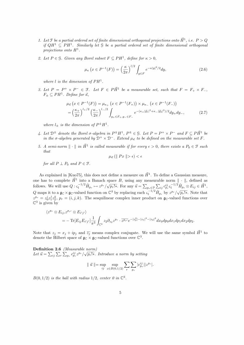
1. Let F be a partial ordered set of finite dimensional orthogonal projections onto ~H1, i.e. P > Qif QH1 ⊆ PH1. Similarly let G be a partial ordered set of finite dimensional orthogonalprojections onto H1.

2. Let P ∈ G. Given any Borel subset F ⊆ PH1, define for κ > 0,

µκ

(x ∈ P−1(F )

)=

( κ

2π

)l/2∫

y∈F

e−κ|y|2/2dy, (2.6)

where l is the dimension of PH1.

3. Let P = P+ × P− ∈ F. Let F ∈ P ~H1 be a measurable set, such that F = F+ × F−,F± ⊆ PH1. Define for ~κ,

µ~κ

(x ∈ P−1(F )

)= µκ+

(x ∈ P−1(F+)

)× µκ−(x ∈ P−1(F−)

)

=(κ+

2π

)l+/2 (κ−2π

)l−/2∫

y+∈F+,y−∈F−e−(κ+|~y1|2+κ−|~y2|2)/2dy+dy−, (2.7)

where l± is the dimension of P±H1.

4. Let D± denote the Borel σ-algebra in P±H1, P± ∈ G. Let P = P+ × P− and F ⊆ P ~H1 bein the σ-algebra generated by D+ ×D−. Extend µ~κ to be defined on the measurable set F .

5. A semi-norm ‖ · ‖ in ~H1 is called measurable if for every ε > 0, there exists a P0 ∈ F suchthat

µ~κ (‖ Px ‖> ε) < ε

for all P ⊥ P0 and P ∈ F.

As explained in [Kuo75], this does not define a measure on ~H1. To define a Gaussian measure,one has to complete ~H1 into a Banach space B, using any measurable norm ‖ · ‖, defined asfollows. We will use Q : ς

−1/21 Hpr 7→ zpr/

√pr!∗. For any ~u =

∑pr∈P

∑ij cij

prς−1/21 Hpr ⊗Eij ∈ ~H1,

Q maps it to a gC×gC-valued function on C3 by replacing each ς−1/21 Hpr by zpr/

√pr!∗. Note that

zpr = zi0z

j1z

k2 , pr = (i, j, k). The sesquilinear complex inner product on gC-valued functions over

C3 is given by

〈zpr ⊗ Eij ,zpr′ ⊗ Ei′j′〉

=− Tr[EijEi′j′ ]1π3

∫

C3z2∂z2z

pr · zpr′ e−|z20 |−|z1|2−|z2|2dx0dp0dx1dp1dx2dp2.

Note that zj = xj + ipj and zj means complex conjugate. We will use the same symbol ~H1 todenote the Hilbert space of gC × gC-valued functions over C3.

Definition 2.6 (Measurable norm)Let ~u =

∑ij

∑r

∑pr

cijpr

zpr/√

pr!∗. Introduce a norm by setting

‖ ~u ‖= supij

supz∈B(0,1/2)

∑r

∑pr

|cijpr||zpr |.

B(0, 1/2) is the ball with radius 1/2, center 0 in C3.

5

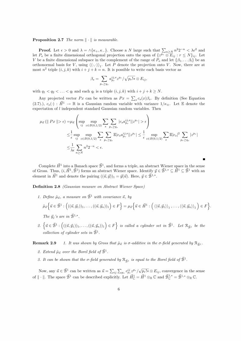
Proposition 2.7 The norm ‖ · ‖ is measurable.

Proof. Let ε > 0 and λ = ∧{κ+, κ−}. Choose a N large such that∑

n≥N n22−n < λε2 andlet Po be a finite dimensional orthogonal projection onto the span of {zpr ⊗ Eij : r ≤ N}ij . LetV be a finite dimensional subspace in the complement of the range of Po and let {β1, . . . βl} be anorthonormal basis for V , using 〈〈·, ·〉〉1. Let P denote the projection onto V . Now, there are atmost n2 triple (i, j, k) with i + j + k = n. It is possible to write each basis vector as

βs =∑

pr≥qs

aij,spr

zpr/√

pr!∗ ⊗ Eij ,

with q1 < q2 < . . . < ql and each qt is a triple (i, j, k) with i + j + k ≥ N .

Any projected vector Px can be written as Px =∑

s cs(x)βs. By definition (See Equation(2.7).), cs(·) : ~H1 → R is a Gaussian random variable with variance 1/κ±. Let E denote theexpectation of l independent standard Gaussian random variables. Then

µ~κ (‖ Px ‖> ε) =µ~κ

sup

ijsup

z∈B(0,1/2)

∑s

∑

pr≥qs

|csaij,spr||zpr | > ε

≤1ε

supij

supz∈B(0,1/2)

∑s

∑

pr≥qs

E|csaij,spr||zpr | ≤ 1

εsup

z∈B(0,1/2)

∑s

E|cs|2∑

pr≥qs

|zpr |

≤ 1λε

∑

n≥N

n22−n < ε.

Complete ~H1 into a Banach space ~B1, and forms a triple, an abstract Wiener space in the senseof Gross. Thus, (i, ~H1, ~B1) forms an abstract Wiener space. Identify ~y ∈ ~B1,∗ ⊆ ~H1 ⊆ ~B1 with anelement in ~H1 and denote the pairing ((~u, ~y))1 = ~y(~u). Here, ~y ∈ ~B1,∗.

Definition 2.8 (Gaussian measure on Abstract Wiener Space)

1. Define µ~κ, a measure on ~B1 with covariance ~κ, by

µ~κ

{~u ∈ ~B1 :

(((~u, ~y1))1, . . . , ((~u, ~yn))1

)∈ F

}= µ~κ

{~u ∈ ~H1 :

(〈〈~u, ~y1〉〉1 , . . . , 〈〈~u, ~yn〉〉1

)∈ F

}.

The ~yj’s are in ~B1,∗.

2.{~u ∈ ~B1 :

(((~u, ~y1))1, . . . , ((~u, ~yn))1

)∈ F

}is called a cylinder set in ~B1. Let R~B1 be the

collection of cylinder sets in ~B1.

Remark 2.9 1. It was shown by Gross that µ~κ is σ-additive in the σ-field generated by R~B1 .

2. Extend µ~κ over the Borel field of ~B1.

3. It can be shown that the σ-field generated by R~B1 is equal to the Borel field of ~B1.

Now, any ~u ∈ ~B1 can be written as ~u =∑

ij

∑pr

cijpr

zpr/√

pr!∗ ⊗Eij , convergence in the senseof ‖ · ‖. The space ~B1 can be described explicitly. Let ~H1

C = ~H1 ⊗R C and ~B1,∗C = ~B1,∗ ⊗R C.

6

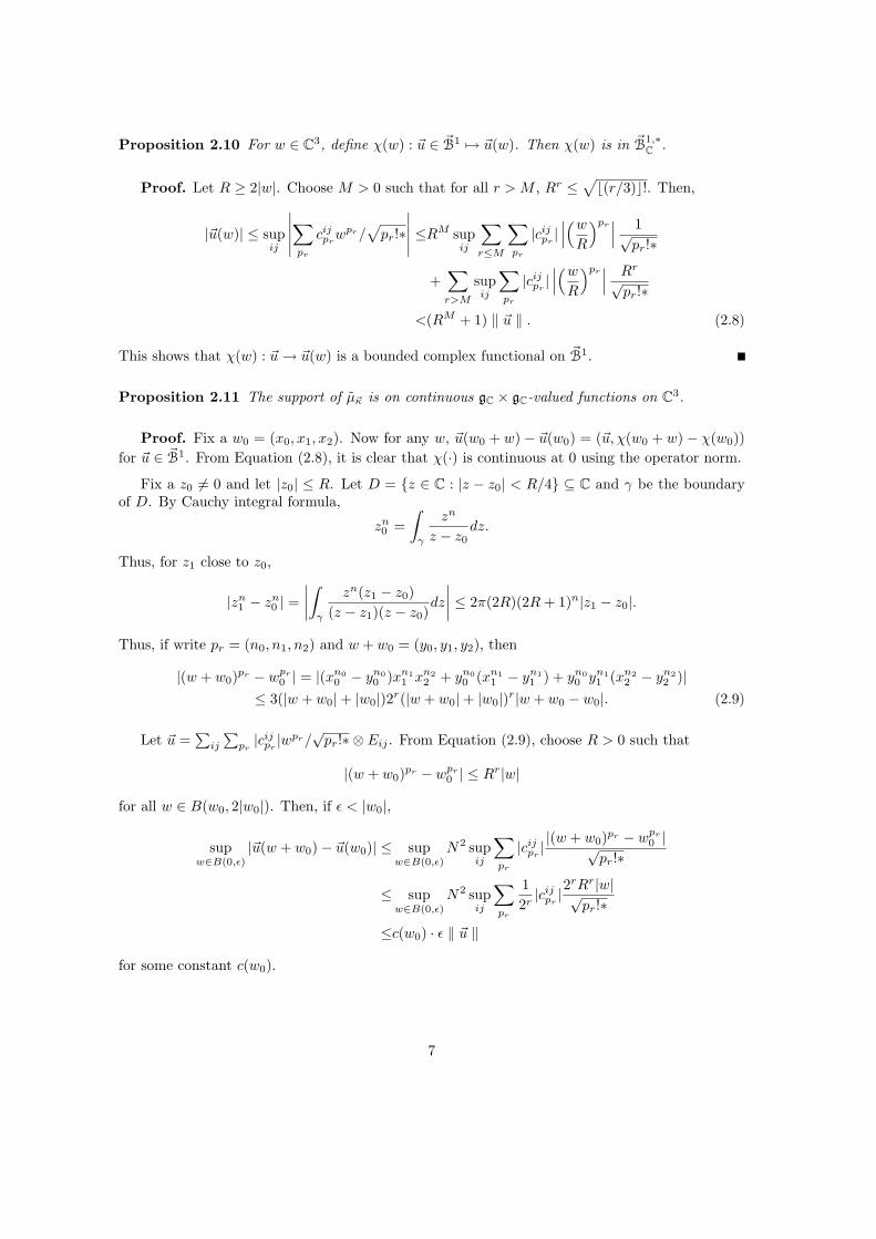
Proposition 2.10 For w ∈ C3, define χ(w) : ~u ∈ ~B1 7→ ~u(w). Then χ(w) is in ~B1,∗C .

Proof. Let R ≥ 2|w|. Choose M > 0 such that for all r > M , Rr ≤√b(r/3)c!. Then,

|~u(w)| ≤ supij

∣∣∣∣∣∑pr

cijpr

wpr/√

pr!∗∣∣∣∣∣ ≤RM sup

ij

∑

r≤M

∑pr

|cijpr|∣∣∣(w

R

)pr∣∣∣ 1√

pr!∗

+∑

r>M

supij

∑pr

|cijpr|∣∣∣(w

R

)pr∣∣∣ Rr

√pr!∗

<(RM + 1) ‖ ~u ‖ . (2.8)

This shows that χ(w) : ~u → ~u(w) is a bounded complex functional on ~B1.

Proposition 2.11 The support of µ~κ is on continuous gC × gC-valued functions on C3.

Proof. Fix a w0 = (x0, x1, x2). Now for any w, ~u(w0 + w)− ~u(w0) = (~u, χ(w0 + w)− χ(w0))for ~u ∈ ~B1. From Equation (2.8), it is clear that χ(·) is continuous at 0 using the operator norm.

Fix a z0 6= 0 and let |z0| ≤ R. Let D = {z ∈ C : |z − z0| < R/4} ⊆ C and γ be the boundaryof D. By Cauchy integral formula,

zn0 =

∫

γ

zn

z − z0dz.

Thus, for z1 close to z0,

|zn1 − zn

0 | =∣∣∣∣∫

γ

zn(z1 − z0)(z − z1)(z − z0)

dz

∣∣∣∣ ≤ 2π(2R)(2R + 1)n|z1 − z0|.

Thus, if write pr = (n0, n1, n2) and w + w0 = (y0, y1, y2), then

|(w + w0)pr − wpr

0 | = |(xn00 − yn0

0 )xn11 xn2

2 + yn00 (xn1

1 − yn11 ) + yn0

0 yn11 (xn2

2 − yn22 )|

≤ 3(|w + w0|+ |w0|)2r(|w + w0|+ |w0|)r|w + w0 − w0|. (2.9)

Let ~u =∑

ij

∑pr|cij

pr|wpr/

√pr!∗ ⊗ Eij . From Equation (2.9), choose R > 0 such that

|(w + w0)pr − wpr

0 | ≤ Rr|w|

for all w ∈ B(w0, 2|w0|). Then, if ε < |w0|,

supw∈B(0,ε)

|~u(w + w0)− ~u(w0)| ≤ supw∈B(0,ε)

N2 supij

∑pr

|cijpr| |(w + w0)pr − wpr

0 |√pr!∗

≤ supw∈B(0,ε)

N2 supij

∑pr

12r|cij

pr|2

rRr|w|√pr!∗

≤c(w0) · ε ‖ ~u ‖

for some constant c(w0).

7

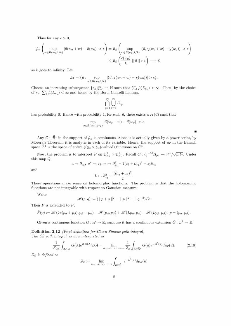
Thus for any ε > 0,

µ~κ

(sup

w∈B(w0,1/k)

|~u(w0 + w)− ~u(w0)| > ε

)= µ~κ

(sup

w∈B(w0,1/k)

|(~u, χ(w0 + w)− χ(w0))| > ε

)

≤ µ~κ

(c(w0)

k‖ ~u ‖> ε

)−→ 0

as k goes to infinity. Let

Ek = {~u : supw∈B(w0,1/k)

|(~u, χ(w0 + w)− χ(w0))| > ε}.

Choose an increasing subsequence {rk}∞k=1 in N such that∑

k µ(Erk) < ∞. Then, by the choice

of rk,∑

k µ(Erk) < ∞ and hence by the Borel Cantelli Lemma,

∞⋂q=1

∞⋃p=q

Erp

has probability 0. Hence with probability 1, for each ~u, there exists a rk(~u) such that

supw∈B(w0,1/rk)

|~u(w0 + w)− ~u(w0)| < ε.

Any ~u ∈ ~B1 in the support of µ~κ is continuous. Since it is actually given by a power series, byMorera’s Theorem, it is analytic in each of its variable. Hence, the support of µ~κ in the Banachspace ~B1 is the space of entire ((gC × gC)-valued) functions on C3.

Now, the problem is to interpret F on ~B1κ+× ~B1

κ− . Recall Q : ς−1/21 Hpr 7→ zpr/

√pr!∗. Under

this map Q,a 7→ ∂z2 , a∗ 7→ z2, τ 7→ ∂2

z2− 2(z2 + ∂z2)

2 + z2∂z2

and

L 7→ ∂2z2− (∂z2 + z2)2

2.

These operations make sense on holomorphic functions. The problem is that the holomorphicfunctions are not integrable with respect to Gaussian measure.

WriteH (p, q) := (‖ p + q ‖2 − ‖ p ‖2 − ‖ q ‖2)/2.

Then F is extended to F ,

F (p) := H (2τ(pα + pβ), pβ − pα)−H (pα, pβ) + H (Lpα, pα)−H (Lpβ , pβ), p = (pα, pβ).

Given a continuous function G : A → R, suppose it has a continuous extension G : ~B1 → R.

Definition 2.12 (First definition for Chern-Simons path integral)The CS path integral, is now interpreted as

1ZCS

∫

A∈A

G(A)eiCS(A)DA = limκ+→i, κ−→−i

1Z~κ

∫

~u∈~B1G(~u)e−iF (~u)dµ~κ(~u). (2.10)

Z~κ is defined as

Z~κ := limκ+→i, κ−→−i

∫

~u∈~B1e−iF (~u)dµ~κ(~u)

8

Remark 2.13 It is not at all clear that such an analytic continuation exists in this definition.We will not address this issue, as in the rest of this article, we will not use this definition at all.Instead, we will give an alternative definition, based on the approach used in [AS97].

3 Wilson Loop Observables

Note that for the rest of this article, κ > 0 is allowed to vary.

Let G be a Lie group. Let {ρk} be any set of finite dimensional representations of G. Theinterest in Chern-Simons path integrals is the evaluation of

Z(R3, Ci, ρi; q) :=1

ZCS

∫

A∈A

l∏

k=1

W (Ck, ρk; q)eiCS(A)DA, (3.1)

where L = {Ck}k is a link in R3 with non-intersecting (closed) curves Ck and

W (Ck, ρk; q)(A) := TrρkT exp

[q

∫

Ck

Aidxi

]. (3.2)

Here, Trρkis the matrix trace in the representation ρk and T is the time ordering operator.

W (Ck, ρk; q)(A) is the holonomy operator of A, computed along the loop Ck. The integral inEquation (3.1) will be known as the Wilson Loop observable (associated to the link L). q will becalled the charge of the link. When L consists of only one curve, the link is termed a knot. Wewill write Z(R3, L; q) ≡ Z(R3, Ci, ρ; q), when ρk = ρ for some representation ρ.

When L is empty, then Z(R3, ∅; q) = 1. The completion of ~H1 is the space of 2-tuple entire(gC × gC-valued) functions on C3, which defines a space of 2-tuple C∞(R3) (gC × gC-valued)functions, i.e.

A ∈ ~B1 7→ A|R3 ∈ (C∞(R3)⊗ gC)× (C∞(R3)⊗ gC).

Using the canonical embedding of R3 into C3, we could use Equation (3.2) to define a function on~B1 and this would give rigorous meaning to Equation (3.1).

There is a second approach to define ZCS, which was used in both [AS97] and [Hah04]. Continuethe same setting as from the previous section. From Equation (2.4), an integration by parts gives,

−ς0

∫

R3Tr [a0 · ∂2a1]dvolR3 , ς0 :=

κ

2π. (3.3)

Define 〈A,B〉0 := −ς0∫

Tr[AB]dvolR3 and (H0, 〈·, ·〉) ≡ H0 := L2g(R3, volR3), the Hilbert space

of g-valued, integrable functions. The Schwartz space S(R3) ⊗ g is dense inside H0 and thus{ς−1/2

0 Hpr

√φκ}pr∈P ⊗ {Eij} forms an orthonormal basis.

Remark 3.1 Let Hpr/√

pr! be the normalized Hermite polynomials with respect to the Gaussianmeasure e−(|x0|2+|x1|2+|x2|2)/2/(2π)3/2dx0dx1dx2. Thus,

ς−1/20 Hpr (x0, x1, x2)

√φκ = ς

−1/20 Hpr (κx0, κx1, κx2)

√φκ/

√pr!.

9

Making use of Equation (2.3), let f1 = ∂2a1. If ~u = (a0, f1), then the Chern-Simons pathintegral is defined as

limθ→i

∫

~u∈~Sg(R3)

ei〈~u〉]+ i2 〈〈~u,~u〉〉0− θ

2 〈〈~u,~u〉〉0Da0Df1. (3.4)

Define ~H0, the completion of ~Sg(R3) using 〈〈·, ·〉〉0, using the same symbol to denote the spaceof gC × gC-valued functions over C3. Define a Gaussian measure µθ on P ~H0 for any P ∈ F as inEquation (2.7). Define ‖ · ‖0:=

√〈〈·, ·〉〉0 and complete the space into ~B0 using a measurable normas before and define a Gaussian measure µθ on ~B0. Denote the paring ((~y, ~u))0 := ~y(~u) ∈ R for~y ∈ ~B0,∗.

To make sense of 〈~u〉] + 〈〈~u, ~u〉〉0 /2 on ~B0, one can define it using polarization and hence definea measure on ~B0. However, in this case, we will use a different approach.

Definition 3.2 Let θ > 0.

1. Suppose F : (0, ε) → C. Do an analytic continuation on F and write F : U ⊆ C → C forsome open and connected set U . Suppose i ∈ U . We will write

limθ→i

F (θ) = F (i).

2. Let P ∈ F, the set of finite dimensional orthogonal projections and let {~e+,k, ~e−,k}k be anorthonormal basis in P ] ~H0. Let y±k = 〈〈·, ~e±,k〉〉0 be the coordinates with respect to ~e±,k. Letthe dimension of P ] ~H0 be 2l.

3. For each k, ~yk = (y+k , y−k ) ∈ R2. Let | · | be the Euclidean distance norm in R2. Define for

each P ∈ F,

Z(P ], θ) :=(

θ

2π

)l ∫

R2l

ei∑l

k=1〈~yk〉]+ 12 |~yk|2e−

θ2

∑lk=1 |~yk|2

l∏

k=1

dy+k dy−k

and Z(P ], i) = limθ→i F (θ).

4. For any continuous cylinder function G ∈ C(P ~H0 → R), define

G({~yk}lk=1) := G

(l∑

k=1

y+k ~e+,k + y−k ~e−,k

).

5. For any continuous cylinder function G ∈ C(P ~H0 → R), let

Z(G,P ], θ)

:=1

Z(P ], θ)

(θ

2π

)l ∫

R2l

G({~yk}lk=1)e

i∑l

k=1〈~yk〉]+ 12 |~yk|2e−

θ2

∑lk=1 |~yk|2

l∏

k=1

dy+k dy−k . (3.5)

Proposition 3.3 Let P ], Q] ∈ F be orthogonal.

1. Z(P ] + Q], θ) = Z(P ], θ)Z(Q], θ).

10

2. For each θ > 0, Z(P ], θ) = (1/√

1− 2i/θ)l. l was defined in Item 2 in Definition 3.2.

3. For each θ > 0, there exists a complex measure νθ such that∫

~u∈~B0 G(~u)dνθ(~u) is given byEquation (3.5) for any cylinder function. Furthermore, |νθ| is a probability measure on ~B0.

4. Let ~s = (s+, s−) ∈ R2 and ~u = (u+, u−) ∈ ~B0,∗ ⊆ ~H0 ⊆ ~B0. Define a product ~s × ~u :=(s+u+, s−u−). The Fourier transform of νθ is given by

Fνθ(s+u+, s−u−) =∫

~B0ei((·,~s×~u))0dνθ

= exp(−i(s+u+ + s−u−)2/2θ2

1− (2i/θ)

)e−

12θ (s+,2u+,2+s−,2u−,2). (3.6)

The RHS can be analytically extended to over C/{0, 2i} and thus

limθ→i

Fνθ(~s× ~u) = e−i〈~s×~u〉] . (3.7)

Remark 3.4 1. If one is interested in only the moment generating function, then∫

~B0e((·,~s×~u))0dνθ = exp

(i(s+u+ + s−u−)2/2θ2

1− 2i/θ

)e

12θ (s+,2u+,2+s−,2u−,2)

andlimθ→i

Fνθ(~s× ~u) = ei〈~s×~u〉] . (3.8)

2. Compare the result of [4] in Proposition 3.3 with Equation (2.5.3) in [AS97], it appears weare off by a minus sign. However, note that the L2 inner product used in that article isnegative of the one used here.

Proof.

1. It follows from 〈~u + ~v〉] = 〈~u〉] + 〈~v〉], ~u ∈ P ] and ~v ∈ Q].

2. The integral

z :=θ

2π

∫

R2eixy+i(x2+y2)/2e−θ(x2+y2)/2dxdy = E[eiZ2/θ], Z ∼ N(0, 1).

But N2 ∼ χ21, and the characteristic function E[eitN2

] = 1/√

1− 2it. Thus, z = 1/√

1− 2i/θand hence the result follows from [1].

3. Let Γ : G ∈ L2(~B0, µθ) → Z(G,P ], θ) ∈ R for any bounded continuous cylinder function G.[1] says that for any cylinder function G, Z(G,P ], θ) is well defined for any P ~H0 such thatG is defined on. Since cylinder functions are dense, this linear functional Γ can be extendedto all of L2(~B0, µθ). From Equation (3.5), Γ has operator norm 1, using the L2 norm onL2(~B0, µθ). By Riesz representation theorem, there exists a complex valued function γθ,|γθ| = 1 such that Γ(G) =

∫~B0 Gγθdµθ.

11

4. Set s+ = s− = 1. Note that ei〈〈·,~u〉〉0 is a cylinder function on P ] ~H0, where P is projectiononto ~u. First assume that P ] = P , i.e. ~u = (u+e, u−e), u+, u− ∈ R and e is a unit vector inH0. Then, a straight forward computation gives

∫~B0

ei〈〈·,~u〉〉0dνθ =√

1− 2i/θE[e

iθ

(N+ iu+√

2θ+ iu−√

2θ

)2]e−( 1

2θ u+,2+ 12θ u−,2),

N is the standard normal distribution. The quantity Q = (N + λ)2 is a non-central χ2

distribution and the characteristic function for Q is given by

exp(

iλ2t1−2it

)√

1− 2it.

Plug in λ = i(u+ + u−)/√

2θ, t = 1/θ,∫

~B0ei〈〈·,~y〉〉0dνθ = exp

(−i(u+ + u−)2/2θ2

1− 2i/θ

)e−( 1

2θ u+,2+ 12θ u−,2).

Observe that u+u− = 〈~u〉]. Take the limit as θ go to i in the sense of Definition 3.2, we havethe result.

Now assume that ~u = (u1p, u2p + tq), with p, q orthonormal vectors in H0 and u±, t ∈ R.Associate + with 1 and − with 2 for convenience. P ] is now spanned by {pj , qj}j=1,2,p1, p2 ≡ p and q1, q2 ≡ q. Then ~u = u1p1 + u2p2 + tq2.

For any arbitrary vector∑

j αjpj + βjqj = y ∈ P ], 〈〈y, ~u〉〉0 = u1α1 + u2α2 + tβ2. If~w = (u1, u2), ~α = (α1, α2) and ~β = (β1, β2), then the integral becomes

(1−2i/θ)(

θ

2π

)2 ∫

R2ei(~w·~α+〈~α〉]+|~α|2/2)e−θ|~α|2/2dα1dα2·

∫

R2ei(tβ2+〈~β〉]+|~β|2/2)e−θ|~β|2/2dβ1dβ2.

Note that 〈~u〉] = u1u2. Apply the calculations above, we get the result.

Definition 3.5 (Second definition for Chern-Simons path integral)Suppose a bounded continuous function G ∈ C( ~H0) can be extended to G ∈ L1(~B0, µθ). Define theChern-Simons path integral as,

1ZCS

∫

A∈A

G(A)eiCS(A)DA := limθ→i

∫~B0

Gdνθ. (3.9)

The existence of νθ was proved in Proposition 3.3.

From Remark 3.4, we note that such an analytic continuation exists, at least for G of the formei((·,~u))0 , ~u ∈ ~B0,∗ ⊆ ~H0 ⊆ ~B0. The Chern-Simons path integral is then interpreted as a linearfunctional acting on (a possibly subspace of) L1(~B0, νθ).

12

3.1 Some Important Comments

Definition 3.5 of the Chern-Simons path integral, is not exact. Write ∂2 = a − a∗. In terms ofHermite polynomials, ∂2 : hk 7→ khk−1 − hk+1. If one does a change of variables, ∂2 : a1 7→ f1 =∂2a1, then Expression (3.4) should become

1det ∂2

∫

~u∈~Sg(R3)

ei〈~u〉]+ i2 〈〈~u,~u〉〉0− θ

2 〈〈~u,~u〉〉0Da0Df1. (3.10)

Of course, det ∂2 does not make sense. It is either 0 or ∞.

Since we are only interested in defining a probability measure, one can just divide out thisindeterminate. But the problem is that there is no way to rigorously justify this division. Thebottom line is that in the second definition of the path integral is far from exact.

Because of this change of variables formula, the definition of the path integral should be

1ZCS

∫

A∈A

G(A)eiCS(A)DA := limθ→i

∫

~a∈~B0G((a0, ∂

−12 a1))dνθ(~a). (3.11)

and the Fourier transform should yield exp[i〈(u0, ∂−12 u1)〉]]. (The adjoint of ∂−1

2 is −∂−12 .) Unfor-

tunately, given u1 ∈ H0, ∂−12 u1 is not in H0.

This change is necessary to get the right knot invariants later on. Actually, one is not interestedin the measure. What one is really after is the Wilson Loop observable. As will be shown later, itis simply a Fourier transform. But Equation (3.6) is not well defined if we make this change.

Fortunately, Equations (3.7) and (3.8) are well defined if 〈(u0, ∂−12 u1)〉] ≡ 〈u0, ∂

−12 u1〉 is defined,

even though ∂−12 u1 is not in H0. Let us be more precise about this statement. We mean that

〈u0 ⊗A, ∂−12 u1 ⊗B〉 := −Tr[AB]

∫

C3(u0 · ∂−1

2 u1)ze−|z|2

2∏

i=0

dxidpi

π< ∞.

Here, z = (z0, z1, z2) and zj = xj + ipj .

Therefore, we will make the following definition:

ECS[e((·,~s×~u))0

]:= e−i〈s+u0,s−∂−1

2 u1〉, (3.12)

for any (u0, u1) ∈ ~B0,∗ with 〈u0, ∂−12 u1〉 < ∞.

A word of caution: On the space of Hermite polynomials, ∂2 = a−a∗ and ∂−12 a1 :=

∫ ·−∞ a1(x2)dx2−∫∞

· a1(x2)dx2. However, on the space of holomorphic functions, ∂2 7→ ∂z2 − z2. The inverse of theoperator is (∂z2 − z2)−1.

If (u0, u1) ∈ ~B0,∗ ⊆ ~H0, then u1 ∈ H0. Under the map Q−1, a1 = Q−1u1 is in L2(R3 → g). Ifa1 is in L2(R3 → g), then

∂−12 a1 =

∫ ·

−∞a1(x2)dx2 −

∫ ∞

·a1(x2)dx2

is bounded, but unfortunately it is not L2 integrable. But,

〈a0, ∂−12 a1〉 =

∫

R3a0 · ∂−1

2 a1dvolR3 < ∞,

13

if a0 is L1 integrable.

So far, we considered the Lie algebra g as a Lie subalgebra in su(N). One can view it asa representation of g in u(N). In fact, our method can be generalized to any semisimple Liealgebra, if there is a representation ρ of g such that the bilinear form 〈A,B〉ρ := −Tr[ρ(A)ρ(B)],Tr is the usual matrix trace, is positive and non-degenerate. In this representation, 〈A,B〉 :=−ς0

∫Tr[ρ(A)ρ(B)]dvolR3 , for A,B : R3 → g.

Definition 3.6 (Third definition for Chern-Simons path integral)Let G be any complex (gauge) Lie group for a trivial bundle E. Let ρ be any finite-dimensionalrepresentation of G, such that the bilinear form 〈·, ·〉ρ defined above is positive and non-degenerate.Define a bilinear form 〈·, ·〉 on H0 as above. If ~φ : ~B0 → R is a bounded linear functional, define

ECSκ,ρ

[e((·,~s×~φ))0

]:= e−i〈s+φ0,s−∂−1

2 φ1〉, (3.13)

~s = (s+, s−) ∈ R2, if〈s+φ0, s

−∂−12 φ1〉 < ∞.

There is a κ dependence in the RHS of the definition, which is not obvious from the notation. Theterm ∂−1

2 is actually dependent on κ. When the representation is clear, ECSκ [·] ≡ ECS

κ,ρ[·].

Note that e((·,~s×~φ))0 is in L1(~B0, νθ). Similar to Definition 3.5, ECSκ,ρ is viewed as a linear

functional, defined only on a strict subspace of L1(~B0, νθ). Since we only need Equation (3.13),we will not find the largest possible subspace in L1(~B0, νθ) for which ECS

κ,ρ can be defined on.

For the rest of this article, our Chern-Simons path integral will be computed using Definition3.6.

4 Abelian Gauge Group

The next thing we want to compute is the Wilson Loop observables for an abelian gauge groupusing Definition 3.6 for Chern-Simons path integral. Write

ψ(z0, z1, z2) = exp[−(z20 + z2

1 + z22)/2], (z0, z1, z2) ∈ C3.

We will write

〈u0, ∂−12 u1〉 =

∫

C3(u0 · ∂−1

2 u1)ze−|z|2

2∏

i=0

dxidpi

π

for u0, u1 : C3 → C. Here, zj = xj + ipj . We will also write

〈f, g〉 =∫

Rk

f(x)g(x)dvolRk .

Here, f, g : Rk → R, k = 1, 2, 3.

We will work out the case for N = 1 for an abelian gauge group G. Let L = {Ck}k be a link,and embed R3 into C3. We assume L is smooth and let lk : [0, 1] → R3 be a parametrization ofCk. We need to do the following 2 scalings:

14

a The link L in R3 ⊆ C3 is scaled by a factor κ/2.

b Given ~a = (a0, a1) ∈ ~B0, we will scale it by√

ς2ψ, ς2 := κ/(4√

2π).

The reader might question why do we need to make these scaling. These factors are necessaryin order to obtain the knot invariants. With these scaling factors, the holonomy operator of ~acomputed along the L is given by

∏

k

W (Ck) = exp

[q√

ς2∑

k

∫

κCk/2

ψ · (a0dx0 + a1dx1)

], ~a = (a0, a1) ∈ ~B0.

The map

~a 7→ √ς2

∑

k

∫

κCk/2

ψ · (a0dx0 + a1dx1)

is linear. Suppose it can be written as ~a 7→ √ς2((~a, ~η(L)))0, whereby ~η(L) ∈ ~B0,∗ ∈ ~H0 and ((·, ·))0

is a pairing.

Using Equation (3.13), the Wilson Loop observable, Equation (3.1) now becomes

Z(R3, L) = ECSκ

[e√

ς2((·,~η(L)))0]

= exp[−iq2ς2〈η(L)0, ∂−12 η(L)1〉0],

~η(L) = (η(L)0, η(L)1). There is a κ dependence on the RHS. We will work out the RHS explicitlyin the following calculations. To obtain the knot invariants, we will have to take the limit as κgoes to infinity.

Lemma 4.1 Continue with the discussion as above. Then,

Z(R3, L) = exp[− πiq2κ3

16π√

2π

∑

j≥k

∫ 1

0

ds

∫ 1

0

dt δkj

[lj,′0 (s)lk,′

1 (t)− lk,′0 (t)lj,′1 (s)

]

· hj(s)hk(t)⟨χ(κlj(s)), ∂−1

2 χ(κlk(t))⟩ ]

,

with δkj = δj

k = 1− (δjk/2) and κ = κ/2.

Proof. Let {lk ≡ (lk0 , lk1 , lk2)} and lk : [0, 1] 7→ R3 be a parametrization of Ck. Write hκk(s) ≡

hk(s) = exp[−κ2lk,2(s)/8] and κ = κ/2. Let {s0 = 0 < s1 < . . . sn = 1} be a partition of [0, 1] and∆is = si − si−1. Let ∆ = supi ∆is. Then, doing a Riemannian sum approximation,

κ

[∫ 1

0

hk(s)a0(κlk(s))lk,′0 (s)ds + hk(t)a1(κlk(t))lk,′

1 (t)dt

]

= lim∆→0

κ

∑

i

hk(si)a0(κlk(si))lk,′0 (si)∆is +

∑

j

hk(tj)a1(κlk(tj))lk,′1 (tj)∆jt

= lim∆→0

κ

~a,

( ∑

i

hk(si)χ(κlk(si))lk,′0 (si)∆is,

∑

j

hk(tj)χ(κlk(tj))lk,′1 (tj)∆jt

)

0

.

15

χ(lk(s)) was defined earlier, a linear functional χ(lk(s)) : a 7→ a(lk(s)), i.e. evaluate a at the pointlk(s) ∈ R3.

Define an operator F such that

F (~a) := lim∆→0

κ

~a,

( ∑

i

hk(si)χ(κlk(si))lk,′0 (si)∆is,

∑

j

hk(tj)χ(κlk(tj))lk,′1 (tj)∆jt

)

0

.

We need to show that F is bounded. Since ~B0,∗ ⊆ ~H0, we can represent F as F = (·, ~η(L))0,~η(L) = (η(L)0, η(L)1), η(L) ∈ ~B0,∗.

From Equation (2.8), since the link L is bounded, thus we can find a M1 such that |χ(t)| ≤ M2

for all t ∈ L. Let M2 be a constant such that |lk,′(s)| ≤ M2. Hence,

κ

∣∣∣∣∣∣

~a,

( ∑

i

hk(si)χ(κlk(si))lk,′0 (si)∆is,

∑

j

hk(tj)χ(κlk(tj))lk,′1 (tj)∆jt

)

0

∣∣∣∣∣∣≤ 4κM1M2|~a|

for any partition. Thus, F is a bounded linear functional on ~B0 and we can write

κ

[∫ 1

0

hk(s)a0(κlk(s))lk,′0 (s)ds + hk(t)a1(κlk(t))lk,′

1 (t)dt

]=(~a, ~η(L))0.

Note that ~η(L) ∈ ~B0,∗, which is embedded in a Hilbert space. Using the unitary map Q, wecan represent η(L)0 as a function in L2(R3, volR3). Likewise for η(L)1. Recall that

∂−12 f(x0, x1, x2) =

∫ x2

−∞f(x0, x1, y)dy −

∫ ∞

x2

f(x0, x1, y)dy. (4.1)

Let w(lk(s)) = Q−1χ(κlk(s)), a real-valued function on R3. Later on, we will show that w(lk(s))is in L1(R3, volR3). See the proof of Lemma 4.2. Under the map Q−1, ~η(L) is represented as

η(L)0 =∑

k

∫ 1

0

hk(s)w(lk(s))lk,′0 (s) ds,

η(L)1 =∑

k

∫ 1

0

hk(s)w(lk(s))lk,′1 (s) ds.

Using Equation (4.1), by Fubini’s Theorem,

∂−12

∫ 1

0

hk(s)w(lk(s))lk,′1 (s) ds =

∫ 1

0

hk(s)∂−12 w(lk(s)) · lk,′

1 (s) ds.

By abuse of notation, using the same symbol ∂−12 to refer to the operator acting on the space of

holomorphic functions, we will write∫ 1

0

hk(s)∂−12 w(lk(s)) · lk,′

1 (s) ds =∫ 1

0

hk(s)∂−12 χ(κlk(s)) · lk,′

1 (s) ds.

In a nutshell, we are justified in exchanging the operator ∂−12 with the integrals.

16

Now, Equation (3.13) gives

Z(R3, L) = ECSκ

[e((·,~η(L)))0

]

=exp

[− πiq2κ3

16π√

2π

⟨∑

k

∫ 1

0

hk(s)χ(κlk(s))lk,′0 (s) ds, ∂−1

2

∑

k

∫ 1

0

hk(s)χ(κlk(s))lk,′1 (s) ds

⟩]

=exp

[− πiq2κ3

16π√

2π

⟨∑

k

∫ 1

0

hk(s)χ(κlk(s))lk,′0 (s) ds,

∑

k

∫ 1

0

hk(s)∂−12 χ(κ · lk(s))lk,′

1 (s) ds

⟩].

Further simplification gives

exp[− πiq2 κ3

16π√

2π

∑

j≥k

∫ 1

0

ds

∫ 1

0

dt δkj

[lj,′0 (s)lk,′

1 (t)− lk,′0 (t)lj,′1 (s)

]

· hj(s)hk(t)⟨χ(κlj(s)), ∂−1

2 χ(κlk(t))⟩ ]

,

with δkj = δj

k = 1− (δjk/2) and κ = κ/2.

The term

κ3

16π√

2π

∫ 1

0

ds

∫ 1

0

dt[lj,′0 (s)lk,′

1 (t)− lk,′0 (t)lj,′1 (s)

] ⟨χ(κlj(s)), ∂−1

2 χ(κlk(t))⟩hj(s)hk(t) (4.2)

should be the linking number between curves lk and lj , provided both curves do not intersect. Tocheck this, we have to first compute

⟨χ(κlj(s)/2), ∂−1

2 χ(κlk(t)/2)⟩e−κ2(lj,2(s)+lk,2(t))/8.

This is where we need to digress a bit. Here, one has to be careful. The Banach space~B0 is the space of C∞(C3,R) ⊗ gC × C∞(C3,R) ⊗ gC. We identify using Q : L2(R3, volR3) →L2(C3, e−|z|

2dω/π3), ω is the standard symplectic form on R6 and

Q : ς−1/20

Hpr (κ·)√pr!

√φκ ⊗ Eij 7→ zpr

√pr!

⊗ Eij . (4.3)

See Remark 3.1. Recall Q sends a∗ 7→ z2 and a 7→ ∂z2 . ∂−12 as an operator on ~B0 is not the same

operator as on L2(R3, volR3).

Furthermore, the linear functional a ∈ R3 : f ∈ L2(R3, volR3) 7→ f(a) is not χa ∈ ~B0,∗. In fact,the completion of L2(R3, volR3) will no longer be functions, but generalized functions, hence sucha linear functional does not make sense on the completion of L2(R3, volR3). Recall we completethe Hilbert space into a Banach space using a weaker measurable norm.

However, one can do an approximation to this functional. When integrated with respect tothe function φκ(· − a) ∈ H0, for large enough κ, 〈f, φκ(· − a)〉 gives a value close to any functionf evaluated at the point a ∈ R3. In fact, it tends to the Dirac function as κ approaches infinity.However, one has to check that it is in the dual of the Banach space containing L2(R3, volR3).

Now, χw =∑∞

r=0

∑pr

zpr wpr/pr!. Since our links lie in R3, we will only consider w real. Anintelligent guess will suggest that

√φ(· − a) should somehow be connected to χ. Thus, we need to

find the corresponding function of χa in L2(R3, volR3).

17

Lemma 4.2 Continue with the discussion as above. Then,

κ3

16π√

2π〈χ(κlj(s)/2), ∂−1

2 χ(κlk(t)/2)〉e−κ2(lj,2(s)+lk,2(t))/8

=κ2

8πe−κ2|Plj(s)−Plk(t)|2/8

⟨κ√4π

e−κ2(·−lj2(s))2/4, 2Φlk2 (t),

√2/κ(·)− 1

⟩,

where Φx2,√

2/κ is the cumulative distribution function of a normal distribution, mean x2 andvariance 2/κ2. P is the projection on R2.

Proof. Q−1 maps χκt/2 to

ς−1/20

√φκ(x)

∞∑r=0

∑pr

Hpr (κx)(κt/2)pr

pr!= ς

−1/20

√φκ(x)eκ2(2x·t−t2)/4eκ2t2/8

for t real, which upon simplification gives ς−1/20

√φκ(· − t)eκ2t2/8. Here, x · t is the usual scalar

product in R3.

In other words, for each t ∈ R3,

Q : ς−1/20

√φκ(· − t)eκ2t2/8 =ς

−1/20

√φκ

∞∑r=0

∑pr

Hpr (κ·)κrtpr

2r · pr!

7→∞∑

r=0

∑pr

zprκrtpr

2r · pr!= χκt/2 ∈ ~B0,∗.

This shows that ς−1/20

√φκ(· − t)eκ2t2/8 is in the dual space of the completion of L2(R3, volR3).

Now ∂−12 f :=

∫ ·−∞ f(x2)dx2 −

∫∞· f(x2)dx2. Thus, Equation (4.2) simplifies to

κ3

16π√

2π〈χ(κlj(s)/2), ∂−1

2 χ(κlk(t)/2)〉e−κ2(lj,2(s)+lk,2(t))/8

=κ3

16π√

2π〈Q−1χ(κlj(s)/2), ∂−1

2 Q−1χ(κlk(t)/2)〉e−κ2(lj,2(s)+lk,2(t))/8

=−1∏

α=0

κ

2√

2πe−κ2|ljα(s)−lkα(t)|2/8

⟨κ√4π

e−κ2(·−lj2(s))2/4,

∫ ·

−∞−

∫ ∞

·

κ√4π

e−κ2|x2−lk2 (t)|2/4dx2

⟩

=− κ2

8πe−κ2|Plj(s)−Plk(t)|2/8

⟨κ√4π

e−κ2(·−lj2(s))2/4, 2Φlk2 (t),

√2/κ(·)− 1

⟩,

where Φx2,√

2/κ is the cumulative distribution function of a normal distribution, mean x2 andvariance 2/κ2. P is the projection on R2. Note also that in the first equality, we made use of thefact that Q−1 preserves the inner product between the two Hilbert spaces.

The term exp[−κ2(x − y)/8] will vanish as κ goes to infinity unless x = y. If lj2(t) > lk2(s),then the integral gives a +1; if lj2(t) < lk2(s), it gives −1. This amounts to giving a + sign toovercrossing and − sign for undercrossing. Otherwise it is zero. Hence the integral along the arcscontribute negligibly to the double integral for large enough κ.

As κ goes to infinity, the integral in Equation (4.2) reduces to a finite sum, assigning +1 toovercrossings and -1 to the undercrossings. It computes the linking number between lj and lk.

18

However, there is more. One has to take into account of the sign of the orientation at eachcrossing. When projected down onto R2, lj,′0 and lk,′

1 form a frame at p. The orientation is givenby sgn(Plj ~×Plk), where ~× is the vector cross product in R2.

Definition 4.3 (Link Diagrams)Assume that a link L = {l1, l2, . . . lm} ∈ R3 is C1 and the individual curves do not intersect oneanother, i.e. lj ∩ lk = ∅ for any j, k. Parametrise each curve, lj = (lj0, l

j1, l

j2) : [0, 1] → R3 such

that |lj,′| 6= 0. Note that in the following definitions, it applies if L is just a knot.

1. Let π : R3 → R2 be the projection on the x − y plane. Define a standard projection of thelink onto R2 if the following conditions are satisfied:

a for any point p ∈ R2, π−1(p) intersects at most 2 distinct arcs in L. p is called a crossingif π−1(p) intersects exactly 2 distinct arcs.

b at each crossing p = lj(s0) = lk(t0), there exists an ε > 0 such that for all |s− s0| < ε and|t− t0| < ε, the vector cross product πlj(s)~×πlk(t) 6= 0, i.e. the 2 arcs at the crossing pare linearly independent.

Denote the set of crossings between curves lj and lk by DP(lj , lk). DP(lj) ≡ DP(lj , lj) willdenote the set of crossings in lj. We will write DP(L) to denote the set of crossings of thestandard projection of the link L.

2. For each curve lj, write the interval [0, 1) as a union of intervals⋃n(lj)

i=1 A(lj)i, where in eachinterval A(lj)i, s ∈ A(lj)i 7→ (lj0(s), l

j1(s)) is a bijection. Write C(lj)i := (lj0(A(lj)i), lj1(A(lj)i)) ∈

R2 be the image of the interval A(lj)i under lj. Without loss of generality, further assumeeach interval C(lj)i

α ≡ ljα(A(lj)i) contains at most one crossing which is an interior point inC(lj)i

α.

3. Given 2 arcs C(lj)i, C(lk)i which intersect at p, define sgn(J(C(lj)i, C(lk)i)) to be the sign ofthe determinant of the Jacobian J(C(lj)i, C(lk)i) = lj,′0 (s)lk,′

1 (t)− lk,′0 (s)lj,′1 (t) at the crossing

p = (lj0(s), lj1(s)) = (lk0(t), lk1(t)). Otherwise, define it to be zero if the 2 arcs do not intersect

at all. We will also write sgn(p; lj : lk) ≡ sgn(J(C(lj)i, C(lk)i)), p = C(lj)i ∩C(lk)i and callthis the orientation of p.

4. Using the same notation as the previous item, for each crossing p ∈ C(lj)i ∩ C(lk)i, define

sgn(C(lj)i : C(lk)i) ={

1, lj2 > lk2 ;−1, lj2 < lk2 .

If the 2 arcs do not intersect, set it to be 0. We will also write sgn(p; lj2 : lk2) ≡ sgn(C(lj)i :C(lk)i) and call this the height of p.

Remark 4.4 The set DP(L) only makes sense for a link diagram projected on R2. Different linkdiagrams will give a different set of crossings. Thus it is not well defined for a link L, but ratheron a link diagram.

Lemma 4.5

limκ→∞

κ3

16π√

2π

∫

A(lj)i

ds

∫

A(lk)i

dt[lj,′0 (s)lk,′

1 (t)− lk,′0 (t)lj,′1 (s)

] ⟨χ(lj(s)), ∂−1

2 χ(lk(t))⟩

· e−κ2(lj,2(s)+lk,2(t))/8

= −sgn(J(C(lj)i, C(lk)i))sgn(C(lj)i : C(lk)i)

19

Proof. Write Λlk2 (t)κ (·) = 2Φlk2 (t),

√2/κ(·)− 1. Then the integral becomes

−∫ 1

0

ds

∫ 1

0

dt[lj,′0 (s)lk,′

1 (t)− lk,′0 (t)lj,′1 (s)

]φκ/2(Plj(s)− Plk(t))

⟨φκ/

√2(· − lj2(s)), Λ

lk2 (t)κ

⟩.

Make a change of variables: Plj : s ∈ A(lj)i 7→ x0 = (lj0(s), lj1(s)) ∈ R2 and yj : x0 7→ lj2(s).

Similarly, Plk : t ∈ A(lk)i 7→ x1 = (lk0(t), lk1(t)) ∈ R2 and yk : x1 7→ lk2(t). Then the integralbecomes (dω = dx0 ∧ dx1.)

sgn(J(C(lj)i, C(lk)i))∫

C(lj)i×C(lk)i

φκ/2(x0 − x1)⟨φκ/

√2(· − yj(x0)),Λyk(x1)

κ

⟩dω

=sgn(J(C(lj)i, C(lk)i))∫

C(lj)i×C(lk)i×Rφκ/2(x0 − x1)φκ/

√2(x2 − yj(x0))Λyk(x1)

κ (x2) dωdx2.

(4.4)

When C(lj)i ∩ C(lk)i = ∅, the integral goes to 0. The only case is when p ∈ C(lj)i ∩ C(lk)i. Wewill only consider the case when yj(p) > yk(p). The other case is similar. Then Equation (4.4)becomes

sgn(J(C(lj)i, C(lk)i))∫

C(lj)i×C(lk)i×Rφκ/2(x0 − x1)φκ/

√2(x2 − yj(x0)) dωdx2

+ sgn(J(C(lj)i, C(lk)i))∫

C(lj)i×C(lk)i×Rφκ/2(x0 − x1)φκ/

√2(x2 − yj(x0))

[Λyk(x1)

κ (x2)− 1]

dωdx2

−→κ→∞ sgn(J(C(lj)i, C(lk)i)).

The last step requires the following explanation: For any |x2 − yj(x0)| < δ, δ small enough,x2 > yk(x1) by assumption. Furthermore, there exists a σ(δ) such that for all κ > σ,

|Φyk(x1),√

2/σ(x2)− 1| < ε

for any given ε.

Definition 4.6 (Algebraic crossing number.)For each crossing p ∈ DP(lj , lk), the quantity sgn(p; lj : lk)sgn(p; lj2 : lk2) is actually well defined onan oriented link diagram, independent of the parametrization used. Denote it by ε(p) ∈ {+1,−1}.

Corollary 4.7 (Linking number between lj and lk.) For j 6= k,

limκ→∞

κ3

16π√

2π

∫ 1

0

ds

∫ 1

0

dt[lj,′0 (s)lk,′

1 (t)− lk,′0 (t)lj,′1 (s)

] ⟨χ(lj(s)), ∂−1

2 χ(lk(t))⟩e−κ2(lj,2(s)+lk,2(t))/8

=−∑

yi∈DP(lj ,lk)

sgn(yi; lj : lk)sgn(yi; lj2 : lk2) := −lk(lj , lk),

the linking number between lj and lk.

There is a problem when j = k. In this case, one has to integrate over the arcs. Thus, thelinking number between lj and itself is ill-defined. The solution as explained in [Wit89] would beto consider a framing vj whereby vj(·) ∈ R3 is a normal vector field along the curve Cj that is

20

nowhere tangent to Cj . Define lj,ε := lj + εvj , ε is some small number. Essentially, lj,ε is a smallshift of lj in a direction vj . The framing vj chosen depends only on the topological class of vj .Then, one computes lk(lj , lj,ε) and take ε going down to zero.

Explicitly, the limit is computed as

limε→0

limκ→∞

κ3

16π√

2π

∫ 1

0

ds

∫ 1

0

dt[lj,′0 (s)lj,′1 (t)− lj,′0 (t)lj,′1 (s)

]

·⟨χ(lj(s)), ∂−1

2 χ(lj(t))⟩

e−κ2(lj,2(s)+lk,2(t))/8.

We will define the above expression as the self-linking number of lj , written as lk(lj , vj).

Remark 4.8 The self-linking number of lj depends on the framing vj.

Taking the sum over all pairs of curves, the Chern-Simons path integral, when N = 1, will givethe linking number of the link for large enough κ.

Corollary 4.9 For an abelian gauge group G with N = 1, the Wilson Loop observable Equation(3.1) for the limit as κ goes to infinity, is given by

Z(R3, L; q) =1

ZCS

∫

A∈A

l∏

k=1

W (Ck; q)eiCS(A)DA

= exp

πiq2

2

∑

j

lk(lj , vj)

exp

πiq2

∑

j>k

lk(lj , lk)

.

References

[AM09] Sergio Albeverio and Itaru Mitoma, Asymptotic expansion of perturbative Chern-Simonstheory via Wiener space, Bull. Sci. Math. 133 (2009), no. 3, 272–314. MR MR2512830

[AS97] Sergio Albeverio and Ambar Sengupta, A mathematical construction of the non-abelianChern-Simons functional integral, Comm. Math. Phys. 186 (1997), no. 3, 563–579. MRMR1463813 (98j:58022)

[FS97] Jurgen Fuchs and Christoph Schweigert, Symmetries, Lie algebras and representations,Cambridge Monographs on Mathematical Physics, Cambridge University Press, Cam-bridge, 1997, A graduate course for physicists. MR MR1473220 (99k:81078)

[Hah04] Atle Hahn, The Wilson loop observables of Chern-Simons theory on R3 in axial gauge,Comm. Math. Phys. 248 (2004), no. 3, 467–499. MR MR2076918 (2005e:81140)

[Hal03] Brian C. Hall, Lie groups, Lie algebras, and representations, Graduate Texts in Math-ematics, vol. 222, Springer-Verlag, New York, 2003, An elementary introduction. MRMR1997306 (2004i:22001)

[Hum78] James E. Humphreys, Introduction to Lie algebras and representation theory, GraduateTexts in Mathematics, vol. 9, Springer-Verlag, New York, 1978, Second printing, revised.MR MR499562 (81b:17007)

21

[Kas95] Christian Kassel, Quantum groups, Graduate Texts in Mathematics, vol. 155, Springer-Verlag, New York, 1995. MR MR1321145 (96e:17041)

[Kuo75] Hui Hsiung Kuo, Gaussian measures in Banach spaces, Lecture Notes in Mathematics,Vol. 463, Springer-Verlag, Berlin, 1975. MR MR0461643 (57 #1628)

[Wit89] Edward Witten, Quantum field theory and the Jones polynomial, Comm. Math. Phys.121 (1989), no. 3, 351–399. MR MR990772 (90h:57009)

22