Chemsep Chemsep HelpHelp
59
Contents Introduction to ChemSep . . . . . . . . . . . . . . . . . . . . . . . . . . . . . . . . . . . . . . . . . . . . . . . . 3 A Brief History of ChemSep . . . . . . . . . . . . . . . . . . . . . . . . . . . . . . . . . . . . . . . . . . . . . . 4 Acknowledgements . . . . . . . . . . . . . . . . . . . . . . . . . . . . . . . . . . . . . . . . . . . . . . . . . . . 5 The Elements of ChemSep’s Interface . . . . . . . . . . . . . . . . . . . . . . . . . . . . . . . . . . . . . . . . . 6 File Menu . . . . . . . . . . . . . . . . . . . . . . . . . . . . . . . . . . . . . . . . . . . . . . . . . . . . . . . . 9 Edit Menu . . . . . . . . . . . . . . . . . . . . . . . . . . . . . . . . . . . . . . . . . . . . . . . . . . . . . . . . 10 Solve Menu . . . . . . . . . . . . . . . . . . . . . . . . . . . . . . . . . . . . . . . . . . . . . . . . . . . . . . . 11 Analysis . . . . . . . . . . . . . . . . . . . . . . . . . . . . . . . . . . . . . . . . . . . . . . . . . . . . . . . . . 12 Databanks . . . . . . . . . . . . . . . . . . . . . . . . . . . . . . . . . . . . . . . . . . . . . . . . . . . . . . . . 13 Tools . . . . . . . . . . . . . . . . . . . . . . . . . . . . . . . . . . . . . . . . . . . . . . . . . . . . . . . . . . . 14 Problem Solving with ChemSep . . . . . . . . . . . . . . . . . . . . . . . . . . . . . . . . . . . . . . . . . . . . 15 Units . . . . . . . . . . . . . . . . . . . . . . . . . . . . . . . . . . . . . . . . . . . . . . . . . . . . . . . . . . . 16 Title . . . . . . . . . . . . . . . . . . . . . . . . . . . . . . . . . . . . . . . . . . . . . . . . . . . . . . . . . . . 18 Component Selection . . . . . . . . . . . . . . . . . . . . . . . . . . . . . . . . . . . . . . . . . . . . . . . . . . 19 Operation . . . . . . . . . . . . . . . . . . . . . . . . . . . . . . . . . . . . . . . . . . . . . . . . . . . . . . . . 20 Thermodynamic Properties . . . . . . . . . . . . . . . . . . . . . . . . . . . . . . . . . . . . . . . . . . . . . . . 23 Reactions . . . . . . . . . . . . . . . . . . . . . . . . . . . . . . . . . . . . . . . . . . . . . . . . . . . . . . . . 29 Physical Properties . . . . . . . . . . . . . . . . . . . . . . . . . . . . . . . . . . . . . . . . . . . . . . . . . . . 30 Temperature Dependent Properties . . . . . . . . . . . . . . . . . . . . . . . . . . . . . . . . . . . . . . . . . . . 31 Feeds . . . . . . . . . . . . . . . . . . . . . . . . . . . . . . . . . . . . . . . . . . . . . . . . . . . . . . . . . . 33 Degrees of Freedom . . . . . . . . . . . . . . . . . . . . . . . . . . . . . . . . . . . . . . . . . . . . . . . . . . . 34 Pressures . . . . . . . . . . . . . . . . . . . . . . . . . . . . . . . . . . . . . . . . . . . . . . . . . . . . . . . . 35 Heaters and Coolers . . . . . . . . . . . . . . . . . . . . . . . . . . . . . . . . . . . . . . . . . . . . . . . . . . . 36 Efficiencies . . . . . . . . . . . . . . . . . . . . . . . . . . . . . . . . . . . . . . . . . . . . . . . . . . . . . . . 37 Sidestreams . . . . . . . . . . . . . . . . . . . . . . . . . . . . . . . . . . . . . . . . . . . . . . . . . . . . . . . 38 Pumparounds . . . . . . . . . . . . . . . . . . . . . . . . . . . . . . . . . . . . . . . . . . . . . . . . . . . . . . 39 Design . . . . . . . . . . . . . . . . . . . . . . . . . . . . . . . . . . . . . . . . . . . . . . . . . . . . . . . . . . 40 Column Specifications . . . . . . . . . . . . . . . . . . . . . . . . . . . . . . . . . . . . . . . . . . . . . . . . . 44 Flash Specifications . . . . . . . . . . . . . . . . . . . . . . . . . . . . . . . . . . . . . . . . . . . . . . . . . . . 48 Solving the problem . . . . . . . . . . . . . . . . . . . . . . . . . . . . . . . . . . . . . . . . . . . . . . . . . . . 49 Tables . . . . . . . . . . . . . . . . . . . . . . . . . . . . . . . . . . . . . . . . . . . . . . . . . . . . . . . . . . 50 Graphs . . . . . . . . . . . . . . . . . . . . . . . . . . . . . . . . . . . . . . . . . . . . . . . . . . . . . . . . . . 51 McCabe-Thiele . . . . . . . . . . . . . . . . . . . . . . . . . . . . . . . . . . . . . . . . . . . . . . . . . . . . . 54 Solve Options . . . . . . . . . . . . . . . . . . . . . . . . . . . . . . . . . . . . . . . . . . . . . . . . . . . . . . 55 Interface Settings . . . . . . . . . . . . . . . . . . . . . . . . . . . . . . . . . . . . . . . . . . . . . . . . . . . . 58 Tec hnical Background . . . . . . . . . . . . . . . . . . . . . . . . . . . . . . . . . . . . . . . . . . . . . . . . . 59 1
Transcript of Chemsep Chemsep HelpHelp

7/27/2019 Chemsep Chemsep HelpHelp
http://slidepdf.com/reader/full/chemsep-chemsep-helphelp 1/59

7/27/2019 Chemsep Chemsep HelpHelp
http://slidepdf.com/reader/full/chemsep-chemsep-helphelp 2/59
ChemSep Help
Harry A. KooijmanAmsterdam, The [email protected]
Ross TaylorClarkson University, Potsdam, New York [email protected]
Copyright c 2013 by H.A. Kooijman and R. Taylor. All rights reserved. This publication is public domain. No responsibility is
assumed by the authors for any injury and/or damage to persons or property as a matter of products liability, negligence, or otherwise, or
from any use or operation of any methods, products, instructions, information, or idea’s contained in the material herein. The use of general
descriptive names, registered names, trademarks, etc. in this publication does not imply, even in absence of specific statement, that such
names are exempt from the relevant protective laws and regulation and therefore free for general use.

7/27/2019 Chemsep Chemsep HelpHelp
http://slidepdf.com/reader/full/chemsep-chemsep-helphelp 3/59
Introduction to ChemSep
ChemSep is a software system for modeling distillation, absorption, and extraction operations. ChemSep was designed to be
easy to use by students with no experience of engineering software, while having sufficient flexibility and power to appeal to
expert users. In pursuit of these objectives ChemSepfeatures a menu-driven, user-friendly interface with an integrated help
system and an autopilot mode that leads the novice user through the data input phase. Expert users, however, are not forced
to follow the path taken by the autopilot but can proceed to enter data in any order they wish. ChemSep also allows the user
to save program settings and to define short-cut macro keys; these can be of considerable help in developing a personal, more
efficient way of working within the user interface.
Some of the features of ChemSepinclude:
• Equilibrium and nonequilibrium stage models (Krishnamurthy and Taylor, 1985; Taylor et al., 1994, Taylor and Kr-
ishna, 1993)
• Steady-state and dynamic column models (Kooijman and Taylor, 1995)
• Ability to handle problems with up to hundreds of components and theoretical stages (40 components and 300 stages
in Lite version)
• Ability to handle a variety of units, including SI
• Automatic checking for missing or inconsistent input
• Built in library of components
• Includes a variety of widely used K-value and enthalpy models
• Ability to display flow, temperature, pressure, composition and K-value profiles, as well as McCabe-Thiele, and trian-gular diagrams
• Ability to accept user supplied estimates of flows and temperatures for problems that may be difficult to converge
• Wide range of options for end specifications, including purities
• Physical properties estimation
• Databank manager included
ChemSep is one of the few column simulation packages that feature a nonequilibrium column model. This model requires
many additional physical properties of multicomponent mixtures in comparison with the more commonly used equilibrium
models. Furthermore, models for the mass and heat transfer coefficients, interfacial area, and flow models are needed. Manydifferent models are built into ChemSep; it is also possible for users to add their own models without major difficulties.
ChemSep uses many default choices for physical property models to limit the number of selections the user has to make,
making it very easy to set up the (nonequilibrium) simulation of separation columns. However, the user is encouraged to
validate each model’s range and applicability to the specific problem being simulated. Without doing so, there is no guarantee
that the simulation is a solution to the actual separation problem at hand. This is especially true for the thermodynamic models
selected but also for the physical properties and mass transfer models.

7/27/2019 Chemsep Chemsep HelpHelp
http://slidepdf.com/reader/full/chemsep-chemsep-helphelp 4/59
A Brief History of ChemSep
The ChemSep project was started in February 1988 at the University of Technology Delft in the Netherlands. It all began
as a project to enable chemical engineering students to do simple column simulations on PC’s. The aim was to let students
do these calculations without requiring them to work with (complicated) flowsheeting packages. At that time these packages
lacked interactive interfaces that were as friendly and flexible as we thought they could be. Most such programs also required
a more powerful computer than a PC and were quite expensive, thereby prohibiting students from acquiring their own copy
and doing the calculations at home.
ChemSep was supposed to be an easy to use, self-explanatory program so that students could use it without a manual and
could setup their own simulation in a matter of minutes. The main idea was to provide the student a predefined path where
he is asked for all the required input to do a simulation. For each selection or data entry point there is online help to provide
an explanation of what is required. Before the user can initiated a simulation the user interface checks the input for errors or
possible problems and - in the event that a potential problem was diagnosed - puts him back at the appropriate place to correct
the invalid input. This proved to be very important in enabling students to use the program without a step-by-step manual (a
good thing, for we had not written one). In fact, it took 4 years for us to write the first manual - and we remain unconvinced
that many people read it.
ChemSep had to be a small program, for it needed to fit on two 360-kilobyte floppy disks (this limit was imposed by the
PCs at Delft and Clarkson universities at that time)! The requirements of the program have remained modest over the years,
especially in comparison to other simulation software. We think that this has also contributed to the success of ChemSep for
it is able to run on old as well as new PC hardware.
ChemSep (v0.92) was introduced to graduate and undergraduate students at TU Delft in September 1988 by Professor J.A.
(Hans) Wesselingh of TU Delft (now at the Rijks Universiteit Groningen in The Netherlands). The use of ChemSep by
Professor Hans in the courses he taught was of enormous value to us in improving the programs. As a result of the success
enjoyed by the program during those first courses at Delft, we continued to develop ChemSep. In March of 1991, when thenonequilibrium model was added, the source code of the user interface as well as the calculation programs was completely
rewritten. With this revision, the simulation files underwent a metamorphosis as well: they were made readable by human
beings, allowing others to use them in further calculations. The result was a completely new and more powerful interface
(with a similar ”look and feel”). This new version, 2.0, was first used in courses at the University of Amsterdam and at
Clarkson University in Potsdam, New York in September 1991. As from October 1992 we started licensing ChemSep to
universities through the CACHE Corporation. More than 80 universities on all inhabited continents have used ChemSep!
Since the first version in 1988 we have been able to steadily add new features:
• v2.0 Nonequilibrium Model (1991),
• v3.0 Liquid-Liquid Extraction (1995),
• v4.0 Reactions and Dynamics (2000),
• v5.0 Windows GUI and CAPE-OPEN Compliancy (2005), and
• v6.0 Parametric Study and User Hydraulic and MTC Models (2006).
We hope to continue this list . . .
7/27/2019 Chemsep Chemsep HelpHelp
http://slidepdf.com/reader/full/chemsep-chemsep-helphelp 5/59
Acknowledgements
We would like to express our appreciation to
• Arno Haket, who was co-author of the first version of ChemSep
• Professor Hans Wesselingh was the first to use ChemSep in his classes and courses, and was a great fan of the project
• Peter Verheijen, for bringing us all together in the first place
• Malcolm Woodman of BP for supporting the first industrial use of ChemSep
• Professor J.M. Prausnitz for making available interaction parameters
• Professors R. Krishna, Andrejz Gorak, J.D. Seader, Klaus Moller, and numerous students who used ChemSep and
provided us with feedback
• The CACHE corporation, who help us to distribute ChemSep
• Anybody else that we forgot
In ChemSep we also make use of some free tools:
• GNUplot is a free Open Source plotting program, see www.gnuplot.org
• Lister is a freeware file viewer, part of Total Commander, see www.ghisler.com
Finally, a project like ChemSep requires the appropriate inspiration and support, for which we would especially like to thank
Ina and Theresa.
Harry Kooijman and Ross Taylor

7/27/2019 Chemsep Chemsep HelpHelp
http://slidepdf.com/reader/full/chemsep-chemsep-helphelp 6/59
The Elements of ChemSep’s Interface
In common with many software systems, ChemSep’s interface consists of Windows, Menus, Lists and Spreadsheets. We
will take a look at each of these elements shortly. First, however, we need to know how to move around in the ChemSep
interface.
Navigating ChemSep
Finding your way around the interface may be done using the keys or with a mouse. Actually, even if you use a mouse, you
will still need the keys from time to time. If you have used a mouse with any Windows based interface before, you will know
how to use the mouse with ChemSep. If you haven’t used a mouse before, you won’t be able to work with ChemSep and there
is no point in us telling you how to use it here. The most important keys in ChemSep are the arrows (Up, Down, Left, and
Right), Enter, Escape.
• Up, Down, Left, Right move the cursor in the indicated direction,
• Enter accepts the current menu option or data entry. An extra mouse click will accomplish the same thing.
Other keys that perform special functions include:
• Function keys ( F1-F10)
• Alt-key combinations
• Ctrl-key combinations
Menus, Lists and Spreadsheets
ChemSep menus are arranged vertically (with the sole exception of the main menu which is horizontal). Each menu item has
one of its letters highlighted. Pressing that letter will execute the corresponding option. Also, one option in the menu will
be under the cursor. When the cursor is on the option you wish to select, press Enter . The arrow keys, as well as Home and
End , move the highlighted item. To return to the previous menu level press Escape. The Escape key always goes back one
level. Keep pressing Escape and you will get back to the main menu. Lists are similar to menus in that you see a vertically
oriented list of items contained in a box. There are a few subtle differences between menus and lists that must be explained.
Lists may be distinguished from menus by the lack of highlighted letters. Also, it is possible that not all of the list will fit in
the window. If the list is a long one, PgUp and PgDn move the list up or down by the number of lines in the list box but leave
the cursor where it was.
Spreadsheets are used for entering data. Numerical or character data is entered in fields. Many ChemSep spreadsheets have
action buttons above, below, or beside them. For example, there may be an Insert or Delete button. To exercise these actions
click on the button. Some of ChemSep’s spreadsheet fields require you to click on them in order to bring up a list of options
from which you must select one. The State field is of this kind. Many of ChemSep’s spreadsheets have semi-active fields.
That is, a particular field may not be available in all cases. The normal Up, Down, Left , Right are used to move around in
a spreadsheet. Some spreadsheets are too large to fit in the available window. You can then use PgUp, PgDn, Ctrl-PgUp
and Ctrl-PgDn to scroll (part of) the spreadsheet up or down or use the mouse to drag the slider at the side or below the
spreadsheet. A spreadsheet that is too large to fit on the screen can be easily identified.

7/27/2019 Chemsep Chemsep HelpHelp
http://slidepdf.com/reader/full/chemsep-chemsep-helphelp 7/59
While using ChemSep you often have to enter a string of characters; the title of a graph, for example, or the numerical value
of some quantity in a spreadsheet field. Position the cursor over the field where you wish to type in a new entry (or change an
old one). Simply start typing the new value. It may sometimes be more convenient to change an existing data entry. With the
cursor on the relevant field, press Enter to get into Edit mode. You can then use the arrow keys Left , Right , Home, and End
to move around, Backspace to delete the character to the left of the cursor and Del to delete the character under the cursor.
Ins toggles between insert and overwrite modes. An asterisk (*) in a spreadsheet field indicates an Unset parameter. With the
cursor on a spreadsheet field displaying a *, press Enter to display the default value and Enter again to accept it. In addition
to the alpha-numeric keys,
Formula Entry
ChemSep can process algebraic calculations wherever numerical input is required. This is useful since, if you don’t know the
actual numerical value that should be entered but you know how to calculate it, you may enter the calculation. Numerical
formulae may include the four basic arithmetic operations, +, -, *, and /. Operations may be nested within parentheses () as
well. When you have typed in the formula, press Enter to evaluate the result and Enter a second time to accept that result.ChemSep does not remember formula entries, only the final result so you may edit the formula until you press Enter.
Here are some examples of numerical formula entry:
3
5-2
(2-1) * (5-2)
All of these result in the number 3. Formula entry can be useful in the feed spreadsheet where you are asked to enter the
component flows. Perhaps you know the total flow rate and the mole fractions rather than the component flows. Instead
of using your calculator to compute the component flows, you can let ChemSep do the calculations for you. By way of an
example consider a column with a feed flow of 573 mol/s containing 36.5 mole percent ethanol, the rest being water. The
component feed flows of ethanol and water could be typed in as:
573 * 0.365
573 * (1 - 0.365)
Units Entry
ChemSep data entry fields also accept units. This feature is particularly useful if you know a quantity in some units other
than the current set of units. Simply type in the numerical value of the quantity and follow the number with its units. The
number will be displayed in the default units. For example, what if the default flow units are kmol/s but we know the feed
flows in lbmol/h? Simply type in the feed flow as, for example, 375lbmol/h and ChemSep will automatically convert thenumber to the correct value in the default set of units. You can use this feature in any data entry field in ChemSep. Spaces
are ignored when evaluating the expression with units. ChemSep checks the dimensions of the units you enter and displays a
warning message if they do not have the correct dimensions. ChemSep recognizes the standard prefixes for multiples of 10.
For example: mmol/s is recognized as (mol/s) / 1000. A numerical formula and a unit string can be entered in the same field
at the same time. All results of formula and unit entry are displayed in the default set of units.
The Keys to ChemSep
The most important keys in ChemSep are Up, Down, Left , Right , Enter . To make life easier for our users we have assigned

7/27/2019 Chemsep Chemsep HelpHelp
http://slidepdf.com/reader/full/chemsep-chemsep-helphelp 8/59
special functions to the F-keys and a number of Alt-key and Ctrl-key combinations. In addition, it is possible to assign your
own functions to the Alt, Shift and Ctrl F-keys.
The F-keys
Some F-keys have special functions assigned to them. Here is a summary:
• F1: Help
• F5: Next input panel
• F6 : Previous input panel
These keys can be pressed wherever you are within the ChemSep interface. F1 may be pressed any time you are in the
ChemSep interface to display a window containing help messages. The message displayed when F1 is pressed depends on
where you are in ChemSep. Press Escape to clear any Help message. The Help system is extensively cross-referenced. Many
help messages and the index contain one or more underlined words. These are hyperlinks that you can click to move to the
help text that relates to the highlighted keyword.
Alt-Key assignments
As is more or less standard practice in menu-driven software, the various items on the main menu can be accessed by holding
down the Alt key and pressing the highlighted letter associated with that item. For example:
• Alt-F jump to the File Menu
• Alt-E jump to the Edit menu
Some other special functions have been assigned to Alt-key combinations:
• Alt-X¡ Exit ChemSep safely (from anywhere)
• Alt-S Solve current problem (avoiding the use of the Solve item of the Input menu)
• Alt-Q Quick solve (also while avoiding the use of the Solve item of the Input menu)
The difference between these last two two-keys is that if you press Alt-S you will be asked to verify the data file name before
any existing file is overwritten. If you press Alt-Q, automatic data checking is ignored and the current file name is overwritten
immediately. The Alt-keys can be pressed from anywhere within ChemSep.
Control key assignments
Some special functions have been assigned to Ctrl-key combinations. For example:
• Ctrl-O opens a new ChemSep Window with the selected sep file.
• Ctrl-N opens a new ChemSep window.
The Ctrl-keys can be pressed from anywhere within ChemSep.

7/27/2019 Chemsep Chemsep HelpHelp
http://slidepdf.com/reader/full/chemsep-chemsep-helphelp 9/59
File Menu
The File Menu can be reached by clicking on File or by holding down Alt-F . It contains the following items:
New Opens a new ChemSep window. Ctrl-N does the same thing.
Open Opens a new ChemSep window after prompting you for a file to open. Also Ctrl-O.
Load Loads a ChemSep problem file from disk into the currently open window.
Reload Reloads the current sep file (useful for recovering from unsaved changes to the input).
Save Saves current data in a file. Prompts for a file name if data has not yet been saved.
Save as Saves current data into a file with a name different to that of the current file.
Close Resets any Input to default values and clears all Results.
Export results ChemSep can write tables (and sometimes graphs) in a variety of formats including csv (Excel) and html.
Print Prints the current table.
Print setup The standard Windows printer setup option.
View file View the contents of files using a file viewer.
Edit file Load a file into a text editor or word processor.
OS shell This option gives you access to the operating system so that you can execute a command not available in ChemSep.
Exit Quits ChemSep after it has prompted you to save the current problem to disk if it wasn’t saved yet. Alt-F4 accomplishesthe same thing.
Several of these options will bring up the standard directory features of Windows. The directory allows you to move around
the file system and select files in the normal way. SEP is the default extension used by ChemSep for all problem files. The
Open, Load, Save, and Save as options will directory list of all files with the extension SEP. You can change the extension by
clicking on the ”Files of Type” drop down list in the Directory. The View option of the File menu allows you to view files on
your disk. After selecting the view option a directory window appears asking you for the name of the file to view. Select the
file you wish to view in the usual way. The edit option is very similar to the view option except that the file is loaded into a
text editor. The default editor is notepad but you can change this in the Interface Settings optio nunder tools. The OS shell
option of the File menu allows you to shell out to the operating system (in our case DOS). This is particularly useful if you
want to execute a DOS command that cannot be executed from the File menu. To pen a DOS window select the OS Shell
option. Type ”exit” and press Enter to close the OS shell window.
7/27/2019 Chemsep Chemsep HelpHelp
http://slidepdf.com/reader/full/chemsep-chemsep-helphelp 10/59
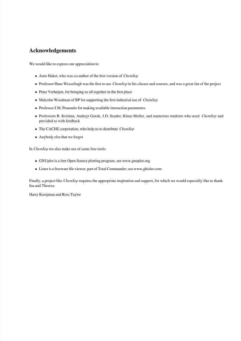
Edit Menu
The Edit menu allows the following actions:
Cut Cut selected items from the current Windows (Ctrl-X does the same thing)
Copy Copy selection Ctrl-C does the same thing)
Paste Paste items last selected by a Copy command at the current cursor postion
Delete Delete selected items (Delete key does the same thing)
Select All Select everything in the current window or input field ( Ctrl-I )
Previous Sheet Move to the prior input/output panel (F5)
Next Sheet Move to the next input/output panel (F6 )
New with Stream Opens a new ChemSep window using one of the streams of the current simulation with the same compo-
nent and properties selections

7/27/2019 Chemsep Chemsep HelpHelp
http://slidepdf.com/reader/full/chemsep-chemsep-helphelp 11/59
Solve Menu
The Solve menu allows the following actions:
Check Input Checks input data for consistency.
Check and Solve Checks input data and runs the simulation program ( Alt-S does the same thing).
Quick Solve Runs the simulation program only - does not check input ( Alt-Q does the same thing)

7/27/2019 Chemsep Chemsep HelpHelp
http://slidepdf.com/reader/full/chemsep-chemsep-helphelp 12/59
Analysis
The Analysis menu allows the following actions:
Plot File Allows you to select a file to plot
Parametric Study Here you can monitor the effect of varying specifications
Stream Curve Plot Stream Curves (UNDER DEVELOPMENT)
Phase diagrams Plot binary and ternary phase diagrams
Residue Curve Map Plot Residue Curve Map
Property diagrams Plot binary and ternary property diagrams
Graphs Quick link to some common plots
McCabe-Thiele Link to the McCabe-Thiele diagram

7/27/2019 Chemsep Chemsep HelpHelp
http://slidepdf.com/reader/full/chemsep-chemsep-helphelp 13/59
7/27/2019 Chemsep Chemsep HelpHelp
http://slidepdf.com/reader/full/chemsep-chemsep-helphelp 14/59
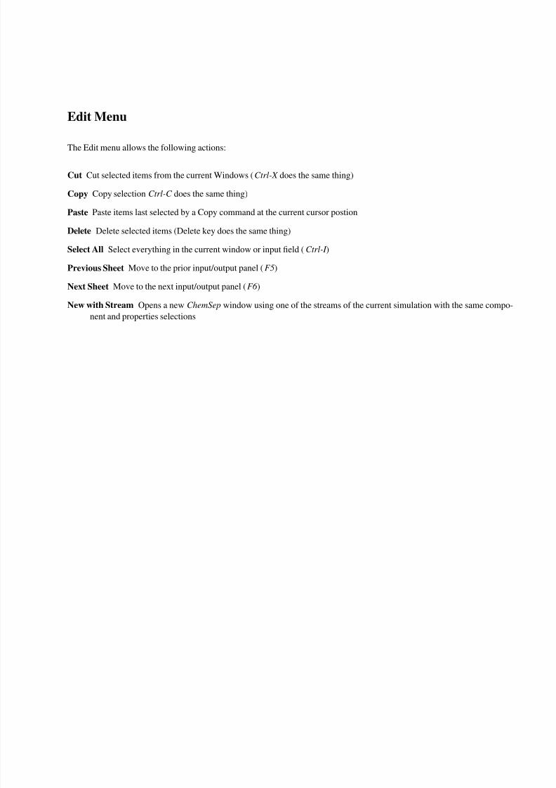
Tools
Interface Settings Pops up a panel where you can change important interface settings. Examples include the number of
significant digits to display, and whether or not to allow ChemSep to create backup files automatically.
Configure Tools Permits user to edit the button bar as well as the use the use of external programs (for example: ChemSep
comes with a separate units conversion program).
Load options Load a ChemSep configuration file.
Save options¡ Save your preferences so that they will be used the next time you call on ChemSep.
Model Developer Starts ChemSep program for adding new models to describe column internals. Requires Fortran Compiler.
Not available in all versions of ChemSep.
Selected Tools are listed at the bottom of this menu.
7/27/2019 Chemsep Chemsep HelpHelp
http://slidepdf.com/reader/full/chemsep-chemsep-helphelp 15/59
Problem Solving with ChemSep
Specifying problems and inspection of simulation results is done with the menu tree on the left hand side of the main ChemSep
window. The menu tree contains the following branches:
Title
Components
Operation
Properties
Thermodynamic properties
Reactions
Physical properties
Feeds
Specifications
Analysis
Pressures
Heaters/Coolers
Efficiencies
Sidestreams
Pumparounds
Design
Column Specificaitons
Flash Specifications
Results
Tables
Graphs
McCabe-Thiele
FUG
Units

7/27/2019 Chemsep Chemsep HelpHelp
http://slidepdf.com/reader/full/chemsep-chemsep-helphelp 16/59
Units
ChemSep is an engineering program and, therefore, requires units to express numerical results. ChemSep allows you to use a
wide variety of units for entering and displaying results. All internal calculations are carried out in SI units but are converted
to the units of your choice for display purposes. You may change the default units by clicking on Units in the tree menu to
the left of the main ChemSep window.
In the left hand column of the table in the Units panel are the names of the quantities whose units you can set. To the right
is the currently selected unit. To change a currently selected unit click in the space that shows the unit name to be changed.
Click on the down arrow to display a list of alternative units that ChemSep recognizes. Use the cursor keys or mouse to
choose the new unit. All quantities that require this unit will be displayed in the newly selected unit until you change it again.
Selected units are saved in ChemSep files so the currently selected units may be changed when you load another file.
The units of measure can be specified for the following quantities: Temperature, Molar flow, Mass flow, Pressure, Energy,
Enthalpy, Composition, Length, Inverse length, Area, Volume, Mass, Angle, Velocity, Surface tension, Density, Diffusivity,
Interaction (parameters), , , and . ChemSep recognises the following units
ChemSep recognizes the standard prefixes for multiples of 10 and they can be used in Other units. For example: ”mm” is
interpreted as ”m/1000”. 2 lists all the prefixes recognized by ChemSep. All units and their prefixes can be typed in data entry
fields as well as selected to be part of the default unit set.

7/27/2019 Chemsep Chemsep HelpHelp
http://slidepdf.com/reader/full/chemsep-chemsep-helphelp 17/59
Table 1: Units of measure
Symbol Unit Symbol Unit
kg kilogram lbf poundforce
m meter kgf kilogramforce
s seconds atm atmosphere
K Kelvin psia lbf/square inch
kmol kilomole psig lbf/sqin gauge
rad radian yd yard
N Newton ton ton
Pa Pascal USton USton
J Joule oz ounce
W Watt lbmol poundmole◦ degree mol mole
lb pound erg erg
g gram dyn dyne
min minute P Poise
h hour mi mile
day day ◦F Fahrenheit
UKgal UKgallon ◦C Celcius
USgal USgallon F Fahrenheit
l liter C Celcius
cal calorie R Rankine
Btu BritishThermalUnit bbl barrel
in inch - dimensionless
” inch % percentft feet %% per thousand
torr torr ppm parts/million
bar bar ppb parts/billion
barg bar gauge
Table 2: Units prefices
Prefix Name Factor Prefix Name Factor
T Tera 1012 d deci 10−1
G Giga 109 c centi 10−2
M Mega 106 m milli 10−3
k kilo 103 mu micro 10−6
h hecto 102 n nano 10−9
da deka 101 p pico 10−12
f femto 10−15

7/27/2019 Chemsep Chemsep HelpHelp
http://slidepdf.com/reader/full/chemsep-chemsep-helphelp 18/59
Title
The Title page is for making notes about the simulation. The information recorded on this page is saved along with all
other input, but is not used in any calculations. It is not necessary for you to specify a title or write anything else about
the simulation. However, it can often be useful to record why this simulation was done in the first place along with steos
necesasry to aid convergence (in the event that ChemSep did not converge easily). This information is especially valuable if
someone other than the originator is attempting to reproduce the orginal work. ChemSep allows you to define a simulation
title as well as additional comments. The first consists of one line which is stored in the header of each SEP file together with
information when the file was saved last and by whom. The comments are stored in the User Data field that can also be read
by other parts of the program. This enables you for example to use the comments to store measured data points that you later
use to plot under parametric study or binary property or equilbria plots. Most of the time however you can document specific
information; the origin of the problem, for example.
7/27/2019 Chemsep Chemsep HelpHelp
http://slidepdf.com/reader/full/chemsep-chemsep-helphelp 19/59
Component Selection
Components are selected from a list shown on the lower left of the Components panel. Selected components appear in the list
on the right. The name of the databank in which components are to be found appears near the top of the panel. To search other
databanks click on the Browse button next to the databank name field to bring up the Windows file manager. Typically these
databanks are binary formatted files with the .PCD extension. It is possible to load components from more than one databank
and ChemSep stores the library from which components were selected (filename with drive and directory. Do understand that
if you are sending someone else the sep-file, you need to send any non-standard library used along as well). An error will be
generated when you attempt to solve the problem if that specific library is not present on the specified path.
To include a component in the list on the right click on its name in the left hand list of components and click on the
¡i¿Select¡/i¿ button. To remove a component from the list on the right click on its name in the right hand panel and click on
the ¡i¿Remove¡/i¿ button. Components cannot be added to or removed from the list on the left. It is however, possible to
create new databanks that contain pure component data for chemicals not available in the existing databanks. The list on the
right can be re-ordered if desired. Click on the name of a component whose position in the list is to be changed. Then click
on Up and Down buttons until the component appears in the desired location.
Components in the list on the right can be replaced by another component if so desired. Click on the identifier of a component
in the list of selected components that is to be replaced. Then click on a component in the list on the left and click on the
Replace button. If a text string is typed into the Find field the list shrinks to include only those components whose names
include the text string. Components can also be chosen based on other attributes such as their property values, for example.
The advanced search capability is available only after clicking in the Advanced Search checkbox in the top right of the panel.
Components can be identified by their name, formula, or structural formula. It is also possible to simply type any desired text
string to be used as the component label within the program. Many components have the same chemical formula and it is
wise to make sure that the identifiers are unique. To change the identifier click on Tools-Interface Options.

7/27/2019 Chemsep Chemsep HelpHelp
http://slidepdf.com/reader/full/chemsep-chemsep-helphelp 20/59
Operation
Click on one of the buttons in the top half of the Operation panel to select the type of simulation desired. The Operation
panel is largely blank until the user selects a model from the list shown in the upper one third. ChemSep is mainly a single
column simulation program with the added capability of modeling a single equilibrium flash. If a column (equilibrium or
nonequilibrium) is to be modeled the user must provide some details of the column configuration: what kind (if any) of
condenser and reboiler is present, how many stages are to be modeled and the stage location of any feeds, sidestreams and
pumparounds. A schematic diagram of the column appears in the window on the right.
Flash calculations are simple equilibrium calculations with specified feeds and two resulting products (vapour and liquid).
These calculations are often used in plant flowsheet calculations, e.g. for heaters, coolers, condensers, boilers and mixers.
For a flash calculation you must specify the number of feed streams (usually this will be one).
ChemSep can simulate a wide variety of distillation, absorption, and extraction columns, including:
Simple Distillation column is one that is equipped with a condenser, a reboiler, and one feed. There will be two product
streams, the distillate and the bottom product.
Extractive Distillation consists of a column with a condenser, reboiler and two feeds that can enter any stage.
Azeotropic Distillation consists of a column with a condenser, reboiler and two feeds. One of the feeds is to the top stage
of the column.
Simple Absorber/Stripper is a column with fixed feed and product streams at the top and bottom. Only the number of
stages varies.
Reboiled Absorber/Stripper is a column with a reboiler and no condenser. One feed may be entered at any stage in addition
to a liquid feed to the top stage.
Refluxed Absorber/Stripper is a column with a condenser but no reboiler.
Single Column Stage is a column with only one stage, two fixed feeds, and top/bottom products
Simple Extractor consists of a column with at the top and bottom two liquid streams entering and leaving. Only the number
of stages may be varied. Extraction requires three or more components.
Supercritical Extractor allows you to simulate the extractor by using an cubic EOS model to describe the liquid - liquid
equilibria.
Single Extraction Stage is a column with only one stage, two liquid feeds, and two liquid products.
Complex Column The complex column option permits you to design a column with several product streams. The column
may or may not be equipped with a condenser and reboiler.
Total Reflux Column has no feed and no product streams. The column should have both a condenser and reboiler. Most
experimental studies are carried out at total reflux in order to minimize material losses. ChemSep has the ability to
model such columns.
The total number of stages must include the number of model stages plus one each for any condenser and reboiler that the
column may be equipped with.

7/27/2019 Chemsep Chemsep HelpHelp
http://slidepdf.com/reader/full/chemsep-chemsep-helphelp 21/59
Enter the stages with external feed streams. Feed stage locations can be separated by a space or by a comma. More than one
feed can go the same stage. For example: a column with feeds to the 18th and 20th stages will have the following line:
Feed stages 18, 20
If the column has sidestreams you should enter the stage numbers of stages with sidestreams. Sidestream stage locations can
be separated by a space or by a comma. More than one sidedraw can come from the same stage. For example: for a column
with sidestreams from its 3rd and 42nd stages could have the following line
Sidestream stages 3, 42
For a column with pumparounds you need to enter the stage numbers for the pumparounds. Enter first the stage from which
the pumparound is withdrawn, then a ”>” and the stage to which the pumparound is directed. For example: a column with apumparound from the 10th stage to the 3rd stage will have the following line
Pumparound stages 10>3
Condensers
ChemSep allows you to choose from 4 different types of condensers:
Total (liquid product) all of the vapour from the top stage is condensed. A portion of the liquid product is returned to the
column as reflux. This is the default option.
Total (subcooled product) all of the vapour from the top stage is condensed and the condensate cooled below the bubble
point of the mixture. The degrees of subcooling have to be specified om the product specification panel.
Partial (vapour product) has a vapour product. The condensate is assumed to be in equilibrium with the distillate.
Partial (two products) ChemSep allows you to simulate a column that has a condenser with TWO product streams; a
vapour and a liquid distillate. The two product streams are assumed to be in equilibrium with each other. Choose a
partial condenser and add a liquid sidestream from stage 1. If you choose this course, you should be aware that the
reflux ratio is defined as the ratio of liquid reflux to vapor distillate. The liquid product is handled in the same way as
other sidestreams.
None You may also have a column with no condenser. In this case you must provide a liquid feed to the top stage!
Reboilers
ChemSep allows you to choose from 4 different types of reboilers:
Partial has a liquid product (bottoms) that is assumed to be in equilibrium with the vapour stream to the column. This is the
default option.
Total all of the liquid from the bottom stage is vaporized and a portion withdrawn as product (bottoms).

7/27/2019 Chemsep Chemsep HelpHelp
http://slidepdf.com/reader/full/chemsep-chemsep-helphelp 22/59
Total, with liquid product ChemSep provides the option of choosing a total reboiler with a liquid product. The liquid
stream leaving the bottom of the column is split and a portion withdrawn as product. The remainder is sent to the
reboiler. All the liquid passing to the boiler is vaporized and returned to the column.
Superheated It is also permitted to select a reboiler that sends a superheated vapour stream to back to the column. The
degree of superheating must be given on the specifications panel.
None You may also have a column with no reboiler. In this case you must provide a vapor feed to the bottom stage.

7/27/2019 Chemsep Chemsep HelpHelp
http://slidepdf.com/reader/full/chemsep-chemsep-helphelp 23/59
Thermodynamic Properties
In the Thermodynamic Properties panel you must select the methods to be used for computing K-values and Enthalpies.
Depending on your selection of models you may be required to enter selected model parameters. Flash and column simula-
tions require a number of thermodynamic properties:
K-values
Activity coefficients
Equations of state
Vapour pressure
Enthalpy
Process simulation makes extensive use of thermodynamic properties, and they can have a profound influence on the simula-
tion results. Selecting the right models sometimes requires insight and experience from the user.
It is your responsibility to assess whether or not the thermodynamic model you have selected is adequate for your needs
K-values
ChemSep includes the following models for computing equilibrium ratios (aka distribution coefficients, or K-values):
Raoult’s law is suitable only for ideal vapor-liquid systems at low pressures. Examples of such mixtures would include
benzene-toluene and methanol-ethanol. It is worth bearing in mind that if Raoul’s law applies to any particular system
then so do the Equation of State, Gamma-Phi, and DECHEMA models.
Equation of state model (EOS) the K-values are obtained from the ratio of fugacity coefficients in the liquid and vapor
phases. The fugacity coefficients are obtained from an equation of state. This model is, perhaps, most useful for
mixtures of hydrocarbons (with or without light gases) at all pressures. Nonideal systems (e.g. methanol-water) can be
handled with the help of special mixing rules, a subject of considerable current research interest.
Gamma-Phi model for the equilibrium ratios uses fugacity coefficients (obatined from an equation of state) for the vapor
phase and the activity coefficient approach to liquid phase fugacities. This leads to a relatively complicated model that
includes a vapor pressure term and the so-called Poynting correction that accounts form changes in the liquid phase
density at higher pressures. The Gamma-Phi model can be used when dealing with nonideal fluid mixtures. It should
not be selected for systems at high pressures.
DECHEMA model is for non-ideal fluid mixtures (e.g. ethanol-water) at low pressures.The model is so-named because it is
the form of the K-value model used in the extensive compilations of equilibrium data published by DECHEMA. It is
a special case of the Gamma-Phi model in which the fugacity coefficient ratio and Poynting correction are assumed to
be unity. This model is sometimes referred to as the modified Raoult’s law, the modification being the multiplication
of the Raoult’s law K-value by an activity coefficient. The DECHEMA data compilation uses the Antoine equation to
compute the vapour pressures but ChemSep allows you to choose other vapour pressure models if you wish.
Chao-Seader Method is appropriate for mixtures of hydrocarbons and light gases. It is not recommended for nonideal
mixtures. The implementation in ChemSep uses the improvements to the original method developed by Grayson and
Streed. The method uses the Regular solution model for the liquid phase (including the Flory-Huggins correction) and
the Redlich Kwong EOS for the vapour phase. An alternative choice would be the Equation of State option.
Relative volatility model can be used for those (usually ideal) systems for which the relative volatilities are known. You
must enter the volatilities for each component in the system. Think of these parameters as K-values that are constants
(independent of temperature, pressure, and composition). The only constraint is that the volatilities must be greater
than zero. The relative volatilities then are computed directly from the ratios of the specified component volatilities.

7/27/2019 Chemsep Chemsep HelpHelp
http://slidepdf.com/reader/full/chemsep-chemsep-helphelp 24/59
Prausnitz model is a specal cse of the Gamma-Phi model that was the basis of the extensive set of thermodynamic property
calculation methods in Computer Calculations for Multicomponent Vapor-Liquid and Liquid-Liquid Equilibriaby J.
Prausnitz, T. Anderson, and 4 other authors (Prentice Hall, 1980). In their book the model uses the UNIQUAC equation
for the activity coefficients, an extended Antoine-like equation for the pure component standard state fugacities for the
liquid (this property is quite closely related to the vapor pressure), and the Hayden O’Connell method (with chemical
theory) for estimating the fugacity coefficients of the vapor phase. In ChemSep you may select other models. This
model is recommended for nonideal systems especially those that undergo vapor phase association reactions (this
includes systems with carboxylic acids, like acetic acid).
Polynomial for estimating vapor-liquid K-values used in ChemSep is:
K m = A + BT + CT 2 + DT 3 + ET 4 (1)
You must enter the coefficients A-E and the exponent m in the speadsheet. See load data for mor information.
Following your selection of a method for estimating K-values you will be invited to choose an equation of state, and/or
methods to estimate vapor pressures and activity coefficients as needed. For example, Raoult’s law requires you to select only
a vapor pressure model, whereas the Gamma-Phi aproach requires you to select an equation of state, an activity coefficient
model, and a vapor pressure model.
Activity Coefficent Models
Activity coefficients are used by thermodynamicists to account for nonideal behavior of liquid mixtures ar low to moderate
pressures. A number of methods of estimating activity coefficients is available in ChemSep.
Ideal where the activity coefficient of all species are unity.
regular solution model is due to Scatchard and Hildebrand. It is probably the simplest model of liquid mixtures and is incor-porated in the Chao-Seader method of estimating K-values. It is provided here for you to use with other thermodynamic
models if you wish.
Van Laar equation and the Margules equation can be used only for binary mixtures (i = 1, j = 2 and i = 2, j = 1).
Wilson this equation was proposed by G.M. Wilson in 1964. It is a ”two parameter equation”. That means that two inter-
action parameters per binary pair are needed to estimate the activity coefficients in a multicomponent mixture. For
mixtures that do NOT form two liquids, the Wilson equation is, on average, the most accurate of the methods used to
predict equilibria in multicomponent mixtures. However, for aqueous mixtures the NRTL model is usually superior.
NRTL equation due to Renon and Prausnitz and has three parameters. Unlike the original Wilson equation it may also be
used for liquid-liquid equilibrium calculations.
UNIQUAC stands for Universal Quasi Chemical and is a very widely used model of liquid mixtures that reduces, with certain
assumptions, to almost all of the other models mentioned in the list. Like the Wilson equation, it is a two parameter
equation but is capable of predicting liquid- liquid equilibria as well as vapour-liquid equilibria. Two versions of the
UNIQUAC model are available:
Original This is the default option and is to be used if you have obtained interaction parameters from the DECHEMA
series of handbooks.
q-prime The form of UNIQUAC that is recommended for alcohol mixtures. An additional pure component parameter,
q’, is needed. q and q’ are stored in ChemSep’s databank.
7/27/2019 Chemsep Chemsep HelpHelp
http://slidepdf.com/reader/full/chemsep-chemsep-helphelp 25/59
UNIFAC is a group contribution method that is used to predict equilibria in systems for which NO experimental equilibrium
data exist. The method is based on the UNIQUAC equation.
ASOG is a group contribution method similar to UNIFAC but based on the Wilson equation. It was developed before
UNIFAC but is less widely used because of the comparative lack of fitted group interaction parameters.
If you select one of the other models but fail to specify a complete set of the interaction parameters, then UNIFAC is used to
compute any unspecified parameters for the other model.
Enthalpy
ChemSep incorporates the following methods for estimating the enthalpy:
None speaks for itself, no enthalpy balance is used in the calculations. Column calculations will be done on the basis of
constant molar flows between stages. This is acheived in practice by assigning arbitrary constant values to the vaporand liquid phase enthalpies. WARNING: the use of no enthalpy model with subcooled and superheated feeds or for
columns with heat addition or removal on some of the stages will give incorrect results. The heat duties of the condenser
and reboiler will be reported as zero since there is no basis for calculating them.
Ideal in this model the enthalpy is computed from the ideal gas contribution. For liquids, the latent heat of vaporization is
subtracted from the ideal gas contribution.
Excess is a short name for the most complete model available in ChemSep for computing enthalpies. The excess enthalpy is
calculated from the model selected for computing K-values. For example, if the SRK EOS is used for both phases then
the excess enthalpy is computed from the same EOS for both phases. If the DECHEMA model is selected for computing
K-values there is no excess enthalpy for the vapour phase. The excess enthalpy of the liquid phase is obtained from the
activity coefficient model and the latent heat contribution is subtracted from the ideal gas contribution.
Polynomial ChemSep also allows you to estimate the enthalpies from a fourth order polynomial in temperature. If you select
this option you must enter the polynomical coefficients for each component in the data section on the lower half of the
Thermodynamic Properties panel. Two sets of parameters are needed, one for the vapour phase and a second for the
liquid phase.
In general the enthalpy of a mixture may be expressed as by the sum of the ideal contribution and an excess or residual
enthalpy. The latter may be evaluated from an equation of state and, indeed, this is how the enthalpy is calculated in many
simulation programs. In ChemSep, however, if an equation of state model is used for the K-values, the excess enthalpy of
both phases is calculated from an equation of state. If an activity coefficient model is used for the liquid phase, then the excess
enthalpy is computed from the appropriate derivative of the Gibbs excess energy model.
Vapour pressure Models
ChemSep provides the following models for calculating the vapour pressure:
Antoine is a three parameter (A, B, and C ) equation:
ln(P ∗) = A−B/(T + C ) (2)
T is the temperature (Kelvin) and P ∗ is the vapor pressure (Pascals). Note the natural logarithm! This option should
be selected if you are using activity coefficient models with parameters from the DECHEMA series. Parameters for the
Antoine equations for many components are available in the ChemSep data files and need not be loaded.

7/27/2019 Chemsep Chemsep HelpHelp
http://slidepdf.com/reader/full/chemsep-chemsep-helphelp 26/59
Extended Antoine Equation this is a six parameter (A to G) equation:
ln(P ∗
) = A + B/(C + T ) + DT + E ln(T ) + FT G (3)
T is the temperature (Kelvin) and P ∗ is the vapor pressure (Pascals). You must enter the parameters for this model in
the data section on the lower half of the Thermodynamic Properties panel.
The Extended Antoine equation can be used to correlate the vapour pressure over extended temperature ranges and can
be extended beyond the critical point for light gases. The book Computer Calculation of Vapor Liquid and Liquid Liquid
Equilibria by J.M. Prausnitz and others Prentice Hall, 1980) provides parameters for an extended Antoine equation
(used to correlate the pure species fuagacity) for 92 components. These parameters can be loaded into ChemSep by
clicking on the Load Parms button on the lower section of the Thermodynamic Properties panel. These parameters
were designed to be used in a Gamma-Phi K-value model.
Design Institute for Physical Property Research (DIPPR) uses an equation that is a special case of the one shown above
in their extensive correlation of vapor pressure data.
ln(P ∗) = A + B/T + C ln(T ) + DT E (4)
The Lee-Kesler method is a corresponding states model. It uses only critical properties and the acentric factor to predict
the vapour pressure.
Riedel equation is similar to the Lee-Kesler method. Both methods are recommended for nonpolar hydrocarbon systems.
Equations of State
Fugacity coefficients are estimated from an Equation of State (EOS). The fugacity coefficient of an ideal gas mixture is unity.
The two-term Virial equation is included in ChemSep:
Pv/RT = 1 + B (5)
Three methods of estimating the second virial coefficient, B, are available.
Hayden and O’Connell have provided a method of predicting the second virial coefficient for multicomponent vapour
mixtures. The method is quite complicated but is well suited to ideal and nonideal systems at low pressures.
The Hayden-O’Connell method can be used in conjunction with Chemical Theory which can be used for mixtures containing
carboxylic acids. The Hayden-O’Connell option does not include the chemical theory calculations. To force ChemSep to use
Chemical theory you must select it from the EOS list. You must enter the association and solvation parameters in the
spreadsheet available under Load Data.
Tsonopoulous method of estimating virial coefficients is recommended for hydrocarbon mixtures at low pressures. It isbased on an earlier correlation due to Pitzer.
Cubic equations of state are very widely used for computing properties of mixtures. They are most often used for hydrocarbon
mixtures (with or without light gases) but extensions now being developed may mean that we will soon be using this class of
model for non-ideal phase equilibrium calculations.
The Van der Waals Equation was the first cubic equation of state. The basic equation has served as a starting point for many
other EOS. The VdW equation cannot be used to determine properties of liquid phases, thus it may not be selected for the
EOS K-value model. ChemSep provides a number of cubic equations of state for estimating fugacities:
7/27/2019 Chemsep Chemsep HelpHelp
http://slidepdf.com/reader/full/chemsep-chemsep-helphelp 27/59
Redlich Kwong equation is used in the Chao-Seader method of computing thermodynamic properties. It is provided here
for use in other models. The RK equation should not be used to determine properties of liquid phases, thus it may not
be selected for the EOS K-value model.
Soave Redlich Kwong (SRK) is a modification of the Redlich Kwong EOS by Soave and one of the most widely used meth-
ods of computing thermodynamic properties. The SRK EOS is most suitable for computing properties of hydrocarbon
mixtures.
API-SRK Graboski and Daubert modified the coefficients in the SRK EOS and provided a special relation for hydrogen.
This modification of the SRK EOS has been recommended by the American Petroleum Institute (API), hence the name
of this model.
Peng-Robinson is another cubic EOS that owes its origins to the RK and SRK EOS. The PR EOS, however, gives improved
predictions of liquid phase densities.
Model Parameters
For some models you will need to enter the values of key parameters. You can tell if you need to enter parameters because
the lower half of the Thermodynamics panel will remain empty if no parameters need be loaded. As soon as you select a
model for which parameters are needed the lower half of the panel will display a drop down list of models and a spreadsheet
in which to enter parameters for one of te selected models. It is possible that you may need to enter parameters for more than
one model. The drop down list in the bottom half of the Thermodynamics panel shows the models that require interaction
parameters to be loaded into ChemSep. The necessary parameters may be found in a ChemSep parameter library (a file with
a .IPD extension) or can be entered from the keyboard. Click on a name in the drop down list of models to see the parameter
spreadsheet for that model. Each line of the speadsheet for these models lists the name of two components. Enter the binary
interaction parameters in the locations to the right of the component identifiers. Most activity coefficient models and some
equations of state require one, two or three interaction parameters. UNIFAC and ASOG do not require parameters.
Parameters for some models can be loaded from libraries that come with ChemSep. To locate a parameter library click on
the ¡i¿Load¡/i¿ button. Use the file selection window to select the desired parameter library. ChemSep will search the library
for parameters that match the system of interest. Be aware that the libraries do not contain parameters for more than a few
systems of interest. You may also load parameters from a ChemSep parameter library. Click on the Load and use the directory
facility to select a file containing parameters for the model. The parameters files are named after the appropriate model and
have the .IPD extension.
When you select an IPD file it is scanned for the right components. You will get a list of all the parameters found in the
file that match your components. You can tag the parameters you want to load in the rightmost column of the parameter list.
Click on the Load button to load the selected parameters. IPD files are stored as ASCII files. You can read them with the
View option, or modify them with the Edit option. Feel free to use your own ASCII editor. Before modifying a library, it is
best is to make a new library of your own by making a copy of the original under a different name (with an IPD extension!).
Put your name in the comment of the file (after comment=). This comment will be displayed while scanning the library.
Parameters that are not known can be left as *. Unknown activity coefficient model parameters will be generated automatically
by the simulation programs using the group contribution method, UNIFAC. The default value for equation of state parameters
is zero. A correlation developed by G. Gao, J-L. Daridon H. Saint-Guirons, P. Xans, and F. Montel (Fluid Phase Equilibria,
Vol. 74, pp. 85-93, 1992) may be used to estimate unset parameters (those marked by a *). Click on the Correlation button
to fill in any missing equation of state parameters. The correlation was developed for the Peng - Robinson EOS and simple
non-polar hydrocarbons. Be VERY careful if you use it to predict para- meters for other cubic EOS and/or other types of
components! This option is not available for all models.

7/27/2019 Chemsep Chemsep HelpHelp
http://slidepdf.com/reader/full/chemsep-chemsep-helphelp 28/59
Some vapor pressure and enthalpy models require you to enter parameters for each component. The procedure for entering
parameters for these models is identical to that for entering interaction parameters.
It is your responsibility to assess whether or not the thermodynamic model you have selected is adequate for your needs
For more detailed information on the thermodynamic and physical property models in ChemSep see Chapter 10 of the Tech-
nical Reference Section.
7/27/2019 Chemsep Chemsep HelpHelp
http://slidepdf.com/reader/full/chemsep-chemsep-helphelp 29/59
Reactions
ChemSep can accommodate the effect of chemical reactions in equilibrium stage models only. A nonequilibrium model for
columns with reactions is due for later release. Click on the Insert button to add a chemical reaction. You can add as many
chemical reactions as you like by repeatedly clicking on the Insert button. A Reactions table will appear immediately below
the Insert button. You should type the name of each line in this table. To the right of the reactions table is the Reactive
zones table. In this table you will need to enter the first and last stage numbers of those stages on which reaction takes place.
You can have more than one Reactive zone; click on the Insert button above the reactive zones table to add a new reactive
zone. Click on the name of each reaction to display the tables in which data for the reaction will appear. These tables will
appear automatically if there is only one reaction. Click on the Reaction type pull down menu and select Homogeneous or
Heterogeneous reaction. Reactions are assumed to occur in the liquid phase (homogeneous reactions) or in a catalyst that is
only in contact with the liquid (heterogeneous reactions). In the latter case the reaction is considered pseudo-homogeneous.
Click on the Kinetics basis pull down menu and select the basis for the kinetic model. Allowable bases are concentrations,
mole fractions, inverse seconds, and activities. Stoichiometric coefficients must be entered for each component and eachreaction in the first of the reaction tables. Stoichiometric coefficients are negative for reactants, positive for products, and
zero for inerts. The constants for the rate equation are entered in the second of the Reaction tables. Further details can be
found in our tutorial with examples of reactive distillation modelling with ChemSepReaction data can be saved seperately
from the sep file and loaded into other applications as needed.

7/27/2019 Chemsep Chemsep HelpHelp
http://slidepdf.com/reader/full/chemsep-chemsep-helphelp 30/59
Physical Properties
Nonequilibrium model simulations require estimates of a number of physical properties in addition to thermodynamic prop-
erties. When first displayed for a new simulation the Physical Properties panel displays only a checked box that indicates that
all physical properties are to be estimated using the default choices that are built in to ChemSep’s physical properties predic-
tion program. Clear the checkmark in roder to gain the opportunity to select physical properties. You may select methods to
estimate the following physical properties:
• Vapor density (may require selection of an equation of state)
• Liquid density
• Liquid viscosity
• Vapor viscosity
• Liquid thermal conductivity
• Vapor thermal conductivity
• Surface tension
• Vapor phase diffusion coefficients
• Liquid phase diffusion coefficients (mixture and infinite dilution)
In most cases it is possible to select methods both pure component and mixture properties. For more details on the models
available for physical property estimations please consult the Property Models Catalog.

7/27/2019 Chemsep Chemsep HelpHelp
http://slidepdf.com/reader/full/chemsep-chemsep-helphelp 31/59
Temperature Dependent Properties
Many properties can be estimated as simple functions of temperature. ChemSep includes many equations that can be used for
this purpose/ Pure component temperature dependent physical properties from correlations published by the Design Institute
for Physical Properties Research (DIPPR). However, any other quantity that depends on one dependent variable and up to
five parameters may be calculated from the equations provided. The equations available in ChemSep are as hown in 3.

7/27/2019 Chemsep Chemsep HelpHelp
http://slidepdf.com/reader/full/chemsep-chemsep-helphelp 32/59
Table 3: Temperature correlations (t is temperature in Kelvin and tr = t/tc)
Key equation
1 y = a
2 y = a + bt
3 y = a + bt + ct2
4 y = a + bt + ct2 + dt3
5 y = a + bt + ct2 + dt3 + et4
10 expa− b
c+T
11 y = exp a
12 y = exp a + bt13 y = exp a + bt + ct2
14 y = exp a + bt + ct2 + dt3
15 y = exp a + bt + ct2 + dt3 + et4
16 y = a + exp b/t + c + dt + et2
17 y = a + exp b + ct + dt2 + et3
45 y = at + bt2/2 + ct3/3 + dt4/4 + et5/575 y = b + 2ct + 3dt2 + 4et3
100 same as 5
101 y = exp a + b/t + c ln(t) + dte
102 y = atb/(1 + c/t + d/t2)103 y = a + bexp(−c/td)
104 y = a + b/t + c/t3 + d/t8 + e/t9
105 y = a/b1+(1−t/c)d
106 y = a(1− tr)[b + c.tr + d.t2r + et3r]107 y = a + b[(c/t)/sinh(c/t)]2 + d[(e/t)/cosh(e/t)]2
114 y = a2(1− tr) + b− 2ac(1− tr)− ad(1− tr)2 − c2(1− tr)3/3− cd(1− tr)4/2− d2(1− tr)5/5115 y = exp a + b/t + c ln t + dt2 + e/t2
116 y = a + b(1− tr)0.35 + c(1− tr)2/3 + d(1− tr) + e(1− tr)4/3
117 y = at + b(c/t)/tanh(c/t)− d(e/t)/tanh(e/t)
120 y = a− b/(t + c)121 y = a + b/t + c ln t + dte
122 y = a + b/t + c ln t + dt2 + e/T 2
207 same as 10
208 y = 10a−b
t+c
209 y = 10a(1/t−1/b)
210 y = 10a+b/t+ct+dt2
211 y = ab−tb−c
d

7/27/2019 Chemsep Chemsep HelpHelp
http://slidepdf.com/reader/full/chemsep-chemsep-helphelp 33/59
Feeds
For each feed the thermal condition and the component flows must be specified in the Feeds panel. The feed panel has three
parts. In the upper portion the thermal condition of each feed is specified. In the middle section the component flows are
entered. The component flows are added together to give the total flow that is printed in the bottom of the window. Each feed
appears in a separate column. Although the number of feed streams was set in the panel, you can, in fact, add and remove
feed streams in this panel.
The feed stage locations were specified in the Operation window. However, you have the option of changing the feed stage
numbers in this window. Any changes to the feed location made in this window will be reflected in the feed stages line of the
Operation window.
Column simulations require you to say something about how the feed is to be handled. In a real column a partially vaporized
feed will actually go to two different stages. The vapor portion will go the stage above and the liquid portion to the stage
where the feed was assigned. You must decide how two-phase feeds are to be handled by selecting Split, Split-below, or
Not-split. The first of these options sends the light phase (in distillation, the vapor) portion of a feed to the stage above and
the heavy phase (the liquid) to the stage selected. The third option allows both phases of a two-phase feed to go directly to
the stage selected. The second option is for feeds below the bottom of a column with no reboiler.
You must choose one of the following feed state specification options: Temperature and pressure or Pressure and vapour
fraction. It is permitted to specify the vapour fraction as zero (corresponding to a liquid at its boiling point) or unity
(corresponding to a vapour feed at its dew point). It is possible to specify vapour fractions less than zero (subcooled feeds)
and greater than unity (superheated feeds). For liquid-liquid extraction you need to enter the fraction of the feed which enters
as the light liquid phase. The bottom feed should be the light liquid (fraction 1) and the feed to the top of the column should
be the heavy phase (fraction 0) liquid. If you reverse the feeds the nonequilibrium model will stop.
Component feed flows are entered in the centre section of the feed window. Component flows can be entered in either massor molar flow units. Click on the pull down list above the feed streadsheet in order to select mass or molar basis for the feeds.
It is possible to switch from mass to molar units while entering data for the same stream. You may add extra feed streams or
eliminate unwanted feeds using the Insert or Delete options on the bottom line of the feeds window.

7/27/2019 Chemsep Chemsep HelpHelp
http://slidepdf.com/reader/full/chemsep-chemsep-helphelp 34/59
Degrees of Freedom
The number of degrees of freedom is computed as follows:
• Start with 1 for the total number of stages and add two for each stage that is not a condenser or reboiler. The pressure
and heat duty must be specified for all such stages.
• Add 2 degrees of freedom for condensers and reboilers. The necessary specification is the stage pressure. One addi-
tional quantity must also be specified (eg reflux ratio for the condenser and bottoms flow rate for the reboiler).
• For total condensers and two-product condensers, the ”stage” is, in fact, the condenser AND the reflux divider together.
The temperature and pressure in the reflux divider is assumed to be the same as the temperature and pressure in the
condenser and the heat loss from the divider is assumed to be negligible. Analogous arguments apply to stream dividers
adjacent to total reboilers.
• Add 1 more degree of freedom for subcooled and superheated streams.
• Unless the product streams from a total condenser or reboiler are specified as superheated or subcooled, they are
assumed to be saturated. That is, the condensate is at its bubble point and the vapour leaving a reboiler is at its dew
point.
• Add (c+3) for each arbitrary feed. Component feed flows, two of temperature, pressure and vapour fraction and the
stage location must be specified for each free feed.
• Add (c+2) for each fixed feed. Fixed feeds are those that enter on the top stage if it is NOT a condenser and the bottom
stage if it is NOT a reboiler. The location of these streams is fixed and so one degree of freedom is lost compared to
the free feeds.
• Add 2 degrees for each sidestream (location and flow rate or ratio). A sidestream from a two product condenser does
not have a free location and is considered in the condenser specification. This additional product stream is not counted
in the number of sidestreams.
7/27/2019 Chemsep Chemsep HelpHelp
http://slidepdf.com/reader/full/chemsep-chemsep-helphelp 35/59
Pressures
The pressure panel allows you to specify the column pressure profile in one of several different ways. When invoked for a
new problem the window contains stars (*) to indicate items that must be completed. The first star may be for the condenser
pressure. The condenser pressure must be specified (if the column has one). If the column has no condenser the condenser
pressure field will be grayed out.
The column pressure mode option allows you to select the way in which the column pressure profile is specified. You may
make the column pressure the same for all stages, you may specify a pressure profile that varies linearly from top to bottom
of the column. In addition to the top stage pressure you may choose to specify the bottom stage pressure or the pressure
drop per stage. For a nonequilibirum model you have the option of having the pressure profile calculated for you during the
simulation. When you have selected the column pressure mode additional stars (*) will appear to indicate any additional
values that must be provided.
constant pressure assigns all pressures equal to the top pressure. Note that the top stage pressure need not be the same as
the condenser pressure!
fixed pressure drop pressures of the stages will be calculated by applying the specified pressure drop for each stage to the
pressure of the stage above. You need to specify the top pressure and the pressure drop.
bottom and top pressures also assigns a constant linear pressure profile over the column but by specifying the top and
bottom pressures.
estimated pressure drop allows the simulator to compute the pressure drop using hydraulic calculations, using the specified
top pressure. This is only possible for non-equilibrium columns (otherwise a zero pressure drop is assumed).

7/27/2019 Chemsep Chemsep HelpHelp
http://slidepdf.com/reader/full/chemsep-chemsep-helphelp 36/59
Heaters and Coolers
ChemSep requires you to specify a heat duty for the column as a whole (this is heat gained or lost through the column walls)
and to give this heat stream a name. The default name for the column heat duty is Qcolumn. It is most common to assume that
the column heat duty is zero. The specified heat duty is assumed to be equally distributed over all stages except condenser
and reboiler. It can be used to simulate the heat losses to the environment (it is added to the specified stage duties).
You may also specify the heat duty for an exchanger on any stage/tray except for the condenser and reboiler (if present).
The duty of these can be separately specified.
To add a heat exchanger, click on the Insert button to specify the stage/tray. Then enter the stage number and the duty of the
exchanger on that stage (positive for heaters/reboilers, negative for coolers/condensers). You should also give each heat duty
a name. Note that quantities of heat removed from a stage should be given a NEGATIVE sign. If you leave the heat duties
unspecified they will be taken as zero. To delete a exchanger use the Remove option. Click on the exchanger to be removed
and then click Remove. You will be invited to confirm your decision.
ChemSep will let you specify the heat duties of Condenser or Reboiler but, these specifications must be on the column
specifications panel. If you try and specify the heat duty of stage 1 when the column is equipped with a condenser or of
the last stage when that is a reboiler you will see a warning that invites you to choose a valid stage number for your heat
exchanger.

7/27/2019 Chemsep Chemsep HelpHelp
http://slidepdf.com/reader/full/chemsep-chemsep-helphelp 37/59
Efficiencies
Enter the default value of the stage efficiency. This value will be used for all equilibrium stages except condensers and
reboilers and other stages selected in the other option in this menu.
The default value is 1 unless you enter another value. Efficiencies normally are expected to be in the range 0 - 1. It is,
however, possible to enter values greater than 1.
ChemSep allows you to specify efficiencies for individual stages that have values that differ from the default value. Click on
Insert and enter a stage number and efficiency value for those stages with efficiencies that differ from the default value. To
remove a stage efficiency from the list of specific stage efficiencies click first on the row of that stage to be removed and then
click the remove button. You will be asked to confirm the removal.
ChemSep will not you specify the efficiencies of Condensers and Reboilers. These units are assumed to have an efficiency of
unity. If you try and specify the efficiency of stage 1 when the column is equipped with a condenser you will see a warningthat mentions the valid range of stages.
7/27/2019 Chemsep Chemsep HelpHelp
http://slidepdf.com/reader/full/chemsep-chemsep-helphelp 38/59
Sidestreams
If you specified a sidestream on the Column Operation panel you must specify some things about the sidestream.
This spreadsheet identifies the stage from which the sidestream is withdrawn, the phase of the sidestream, whether the total
flow or flow ratio is specified, and the numerical value of the specification. The location of any sidestreams was specified in
the Operation panel but you may change the location of the sidestream here. Any changes made in this panel will be reflected
in the Operation if you return there. To change the sidestream stage locate the cursor on the Stage field and type in the new
stage location.
Select the desired sidestream Phase, vapour, or liquid from the list that appears.
Specification of sidestream flow rates is possible, or you may specify the flow ratio between the sidestream flow and the
interstage flow rate. Click on the Type field and press Enter to bring up a list with these two options. An astersik (*) will
appear in the field adjacent to the option you selected. Type the numerical value of the sidstream flow specification in thatfield. The liquid product of a two-product condenser is considered by ChemSep to be a liquid sidestream from stage 1. Click
on Insert button if you wish to add another sidestream, or use the Delete button and to eliminate a sidestream.

7/27/2019 Chemsep Chemsep HelpHelp
http://slidepdf.com/reader/full/chemsep-chemsep-helphelp 39/59
Pumparounds
If you specified a pumparound on the operation panel, there will be a pumparound option in the specifications section.
Selecting it will load the pumparound specification which works in a way that is similar to the sidestream specification panl.
Here you can specify the stages of the pumparound (these are already filled in but can be changed), the phase to pump around
(for liquids a pump would be used, for vapors a compressor), the type of flow specification (total flowrate or flowratio with
respect to the internal column flow at the stage of withdraw), the flow specification, and the type of heat specification (a
heat duty or a temperature) together with that specification. Often, liquid pumparounds are installed with coolers to increase
the liquid reflux in that secion (introducing subcooled liquid will condense some of the internal vapor flow).

7/27/2019 Chemsep Chemsep HelpHelp
http://slidepdf.com/reader/full/chemsep-chemsep-helphelp 40/59
Design
On the Design panel you select the type of internals and models for each section of your column.
ChemSep automatically allocates different sections for the column in between condenser, feeds, sidestreams, and reboiler.
You can insert or delete extra section with the appropriate button near the top of this panel. When you delete or add a section
ChemSep automatically adapts the first and last stages of each section so that all the stages are allocated to a section.
There is a button Settings that brings up a separate panel where you can read (and/or change) the basic settings and parameter
ranges used in tray and packed column calculations. This section is only for experts.
You can also adapt the sections by changing the first and last stage. Each section can consist of a different type of internals,
trays or packing. To simulate each section you need to select the following models (if required):
• Mass Transfer Coefficients (MTC)
• Liquid phase resistance
• Vapour flow model
• Liquid flow model
• Pressure drop
• Entrainment
or for a Liquid-Liquid extraction column:
• Mass Transfer Coefficients
• Dispersed phase
• Light liquid flow model
• Heavy liquid flow model
• Pressure
• Backmixing
Design mode
To simulate a column for which you do not have a complete design, you can use the design mode. This mode is activated
whenever you do not specify the diameter of a section. The program will design the column simultaneously with the sim-
ulation, using the other available design parameters that were specified if possible. You must specify the design method
parameters and the system (derating) factor to use the design mode.
After a successful column simulation in design mode an import option will become available to import the resulting section
data as input. This is useful for making small changes to the automatic designed sections.
ChemSep supports the following internals for normal (Vapor-Liquid) columns:
7/27/2019 Chemsep Chemsep HelpHelp
http://slidepdf.com/reader/full/chemsep-chemsep-helphelp 41/59
• Bubble cap tray
• Sieve tray
• Valve tray
• Dumped packing
• Structured packing
• Equilibrium stage
Internals for Liquid-Liquid extraction are:
• Sieve tray
• Dumped packing
• Structured packing
• Equilibrium stage
• RDC compartment
• Spray stage
Previously saved internal layout designs can also be loaded from a file. The default extension for this type of files is ILD.
Edit the internals data. If you leave the column diameter as * then the program will automatically start the ”design mode”,
where design is adapted during the simulation according the design method and parameters. The design is derated by the
system factor.
The reset option will reset all the internals data. The defaults option will start the design mode and the save design option
allows you to save the Internals Layout Design (ILD) so you can load it again later.
System (derating) factor
The system factor is used to derate the design to avoid problems caused by foaming and other unforeseen problems. The
default system factor (SF) is unity for nonfoaming systems. The system factor also plays a role in the design of downcomers.
For lower system factors higher downcomer residence time and lower velocity under the downcomer are allowed.
Design method
Three different design methods are available:
Fraction of flooding The column is design to operate at a specified fraction of maximum operating (flooding) conditions.
This immeadiately allows you to determine the overcapacity of the column. The default value is 0.75. The closer
the fraction of flooding is to unity, the more difficult to design the column. This is the default design method and is
commonly used when pressure drop is unimportant.

7/27/2019 Chemsep Chemsep HelpHelp
http://slidepdf.com/reader/full/chemsep-chemsep-helphelp 42/59
Table 4: Example System Factors (SF)
Foaming SF Examples
Non 1.0 Air-water
Slight 0.85-1.0 De-propanizer, H2S stripper
Moderate 0.75-0.85 Crude tower, Oil absorber, Amine/Glycol stripper, De-ethanizer
Heavy 0.5-0.75 Amine/Glycol absorber, MEK column
Stable foam 0.3-0.5 Alcohol synthesis, absorber
Table 5: Available mass transfer coefficient correlations for trays
Bubble-Cap Sieve Valve
tray tray trayAIChE AIChE AIChE
Hughmark Chan-Fair
Zuiderweg
Chen-Chuang
Harris
Bubble-Jet
Pressure drop In certain operations, for example, vacuum distillation, it is pertinent that the pressure drop in the column is
minimized. Actually, the design of these columns is done with specified pressure drops (usually resulting in operation
far below the flooding point). For packings we design the column diameter to give rise to the specified pressure drop.
For trays, we use a fraction of flooding of 0.7, and check if the resulting pressure drop is below specified.
Optimizing To fully optimize the design the following aspects play a role: Cost (diameter and tray spacing), Separation
(NTU’s), Pressure drop, Flexibility. To optimize the design for sieve trays you can specify weight factors for each.
For each of these methods you will need to specify one or more design parameters.
Liquid resistance This option selects whether the mass transfer resistance on the liquid side of the interface is included or
ignored.
Dispersed Phase In liquid-liquid extraction the dispersed phase might be either the light or the heavy liquid. This choice has
an influence on the drop slip velocity and, thus, also on the column performance and its design as well. It is a very importantspecification.
Mass Transfer Coefficient (MTC) models To model the mass transfer in the internals we need models that relate the mass
transfer to the diffusion processes occuring. In the non- equilibrium model we have an interface in between each phase,
and two bulk to interface mass transfer processes. To model these processes theoretical models like the Bubble-Jet model or
empirical models like the AICHE model for trays. The empirical models are usually restricted to specific internal types.
Pressure drop can be estimated by empirical models or specified (fixed) by the pressure menu. For packed columns different
models are available:

7/27/2019 Chemsep Chemsep HelpHelp
http://slidepdf.com/reader/full/chemsep-chemsep-helphelp 43/59
Table 6: Available mass transfer coefficient correlations for packings
Random Structured
Onda 68 Bravo 85
Bravo 82 Bravo 92
Billet + Schultes 92 Billet + Schultes 92
. . . . . .
Table 7: Pressure drop correlations for packings
Random Structured
Fixed Fixed
Ludwig 79 Billet 92Leva 92 Bravo 86
Billet 92 Stichlmair 89
Stichlmair 89 Bravo 92
. . . . . .
Flow models describe the flow in each type of internal, which determines how it is modeled. At the moment the options are
plug flow or completely mixed flow.
Entrainment consists of the liquid entrained in the vapour to next tray above or the vapour entrained in the downcomer
entering the next tray below. These effects can be severe near column flooding or at high downcomer velocity. These effects
are normally ignored but can be included to give a more precise simulation.
Backmixing consists of light liquid that moves downward and heavy liquid that moves upwards in the column. In spray or
RDC columns the back- flows can be so large that they influence the column performance significantly.
7/27/2019 Chemsep Chemsep HelpHelp
http://slidepdf.com/reader/full/chemsep-chemsep-helphelp 44/59
Column Specifications
Operation specifications are required when a condenser and/orreboiler are present. On the column specifications page you
must provide numerical values for certain key variables that you will also select. In addition, you can elect to provide initial
estimates of the reflux ratio (or reflux flow rate) and bottoms product flow rate that are used solely for estimating the flows
and compositions throughout the column.
Condenser/Distillate Specifications
If the column is equiiped with a condenser, one of the items from the list below should be specified.
Reflux ratio is the ratio of the reflux flow to the distillate flow. This specification is one of the easiest with which to obtain
converged solutions. For partial and two-product condensers you should be aware that the reflux ratio is defined as
the ratio of liquid reflux to vapor distillate. A second liquid product (if present) is handled in the same way as othersidestreams.
Condenser heat duty is the amount of heat removed in the condenser. Note that the heat duty is a negative number. The
specification of the heat duty is not recommended unless you have a very good idea of its magnitude.
Temperature of the condenser is equivalent to fixing the boiling point of the top product. This specification option is not
recommended. It is very easy to specify a condenser temperature that cannot be achieved and the calculations will not,
therefore, converge.
Distillate rate This option is recommended as it is ”easy” to obtain a converged solution with this option. However, if this
option is selected it is not permitted to select the bottoms flow rate from the reboiler (if present).
Reflux flow rate As an alternative to the reflux ratio you may specify a value for the reflux flow rate (the flow rate from thecondenser that is returned to the top of the column). This option is recommended as it is ”easy” to obtain a converged
solution with this option.
Flow rate of a component in the distillate the component flow rate is the product of the total flow and the mole fraction. It
may not be easy to obtain a converged solution if this option is selected. It is easy to specify a component flow rate that
cannot be achieved with the system that you have input.
Mole fraction of a component in the distillate It may not be easy to obtain a converged solution if this option is selected.
It is easy to specify a composition that cannot be achieved with the system that you have input.
Recovery of a component in the distillate This option may be useful if you have more than one feed with the same com-
ponents in each feed. Note that the recovery must be entered as a percentage. It may not be easy to obtain a converged
solution if this option is selected. It is easy to specify a value that cannot be achieved with the system that you haveinput.
Fraction of total feed recovered the fraction of the flow of the combined feeds that is desired as the top product. Note that
the fraction must be entered as a percentage.
Split between two components in the distillate ChemSep allows you to specify the ratio of the mole fractions of two com-
ponents in the top product stream. You must select the two components from the list provided as well as the desired
composition ratio. It may not be easy to obtain a converged solution if this option is selected. It is easy to specify a
value that cannot be achieved with the process you have created.

7/27/2019 Chemsep Chemsep HelpHelp
http://slidepdf.com/reader/full/chemsep-chemsep-helphelp 45/59
Degrees of subcooling For a subcooled condenser either the amount of subcooling (in degrees) or the reflux temperature
must be specified.
Flexible specifications Any other column variable
In most cases (with exceptions noted below) only one specification is allowed. Certain combinations of condenser and reboiler
specifications are not allowed.
You may enter estimates of the reflux ratio or the distillate flow rate. You are not required to guess these flows or flow ratio
(ChemSep will supply its own estimate if you fail to provide one). These numbers are used solely as an aid to convergence.
Reboiler/Bottom product Specifications
If a reboiler is included in the flowsheet menu, one of the items from the list below be specified.
Boilup ratio is the the ratio of the vapour returned to the column from the reboiler to the bottoms product flow rate. This
specification is one of the easiest with which to obtain converged solutions.
Reboiler heat duty is the amount of heat added in the reboiler. Note that the heat duty is a positive number. The specification
of the heat duty is not recommended unless you have a very good idea of its magnitude.
Temperature of the reboiler is equivalent to fixing the boiling point of the bottom product. This specification option is not
recommended. It is very easy to specify a reboiler temperature that cannot be achieved and the calculations will not,
therefore, converge.
Bottoms flow rate This option is recommended as it is ”easy” to obtain a converged solution with this option. However, if
this option is selected it is not permitted to select the top product flow rate for the condenser (if present).
Boilup is the flow rate of vapour returned to the column from the reboiler. This option is recommended as it is ”easy” to
obtain a converged solution with this option.
Flow rate of a component in the bottom product The component flow rate is the product of the total flow and the mole
fraction. It may not be easy to obtain a converged solution if this option is selected. It is easy to specify a component
flow rate that cannot be achieved with the system that you have input.
Component mole fraction in the bottoms It may not be easy to obtain a converged solution if this option is selected. It is
easy to specify a composition that cannot be achieved with the system that you have input.
Component recovery the fraction of the total feed of a component that is desired in the bottom product. This option may be
useful if you have more than one feed with the same components in each feed. Note that the recovery must be entered
as a percentage. It may not be easy to obtain a converged solution if this option is selected. It is easy to specify a valuethat cannot be achieved with the system that you have input.
Fraction of total feed in bottoms You may specify the fraction of the flow of the combined feeds that is desired as the
bottom product. Note that the fraction must be entered as a percentage.
Split between two components ChemSep allows you to specify the ratio between the mole fractions of two components
in the bottom product stream. You must select the two components from the list provided as well as the desired
composition ratio. It may not be easy to obtain a converged solution if this option is selected. It is easy to specify a
value that cannot be achieved with the system that you have input.
7/27/2019 Chemsep Chemsep HelpHelp
http://slidepdf.com/reader/full/chemsep-chemsep-helphelp 46/59
Degrees of superheating For a superheated reboiler either the amount of superheating (in degrees) or the boilup temperature
must be specified.
Flexible specifications Any other column variable
Flexible Specifications
To specify any variable other than those listed above you should select Flexible Specifications from the pull down speci-
fications menu. This is an advanced option for experienced users. Needless to say that the use of this specification may
sometimes lead to covergence difficulties as fewer checks for consistency of the input can be done. A flexible specification is
an equation like
RR = 2.5 or D = [400 mol/s]
The specification must done in SI units where the variables have the following units: Pressure (Pa), Temperature (K), Mole
flows (kmol/s), Mass flows (kg/s) To convert units of numbers use square brakets
[400 mol/s] -> 0.4 (kmol/s)
[25 C] -> 298.15 (K)
[2 bar] -> 2e5 (Pa)
The following variables can be used in an equilibrium column simulation: V, L, T, X, Y and in a nonequilibrium simulation:
V, L, Ti, Tl, Tv, X , X i,Y, Yi, Mf, P where Mf is the mass transfer flowrate in molar flow units. Some special variables are:
D = Distillate flow rate (kmol/s)
RR = Reflux ratioXD = Distillate composition (also YD)
B = Bottoms flow rate (kmol/s)
BR = Boilup ratio
XB = Bottoms composition (also YB)
WL = Liquid molecular weight (kg/kmol)
WV = Vapour molecular weight (kg/kmol)
MV = Vapour mass flow (kg/s)
ML = Liquid mass flow (kg/s)
MD = Distillate mass rate (kg/s)
MB = Bottoms mass rate (kg/s)
F = Component total feedrate (kmol/s)
The supported operators are: - + * / ‘where ‘is used for exponation. An illegal operation (such as 1/0) will not crash the
program but will result in erroneous results. Curved parentheses can be used to separate terms and force a different order of
evaluation.
Variables also need a stage index:
T1 T on s tage 1
L12 L o n stage 1 2

7/27/2019 Chemsep Chemsep HelpHelp
http://slidepdf.com/reader/full/chemsep-chemsep-helphelp 47/59
Variables like X, Xi, Y, Yi, F require component indices in between curved parenthesis, like:
X2(2) X on stage 2 of 2nd component
Y20(Propane) Y-propane on stage 20
Mass flows can be specified by multiplying the molar variables with the molecular weight of the appropriate phase, for
example:
WL1 * D = [4 kg/s]
or using the special variables
MB = [5000 kg/h]

7/27/2019 Chemsep Chemsep HelpHelp
http://slidepdf.com/reader/full/chemsep-chemsep-helphelp 48/59
7/27/2019 Chemsep Chemsep HelpHelp
http://slidepdf.com/reader/full/chemsep-chemsep-helphelp 49/59
Solving the problem
When you have completed the input of all data, you are ready to solve the problem.
To execute the calculation program you may carry out one of the following actions:
1. Click on the calculator icon located on the icon row
2. Click Alt-s
3. Click Alt-q
The second and third of these options also are available from the Run menu.
The difference between these last two two-keys is that if you press Alt-s all input data will be checked for completeness
and you will be asked to verify the data file name before any existing file is overwritten. If you press Alt-q, automatic data
checking is ignored and the current file name is overwritten immediately.These Alt-key combinations can be pressed from
anywhere within ChemSep.
Unless you press Alt-q, ChemSep checks for any missing or obviously inconsistent data prior to actually carrying our any
calculations. Message boxes informing you of any such oversights will appear only as needed and you will be taken directly
to the place where you should enter the missing data. If you changed something (either by accident or by design) you may
see a warning message if your change leads to some inconsistency that the program can detect. Once the data are verified (or
the checks are bypassed with Alt-q), ChemSep writes the input to a file.
If the input has not been saved in a file prior to the first invocation of the calculation program, ChemSep will insist that you
save the data in a file with a name and directory location of your choosing.
What will happen next is that ChemSep calls up the appropriate simulation program to solve the problem. A new window
opens in which the simulation program writes messages there to let you know the current status of the calculations. Consult
the Solve options for more information on this topic. If you are using the default settings (only iteration numbers written to
the screen) the window will look something like it does here.
When the calculations are complete, the program will inform you of this fact, the interface reloads the input data together
with any Results. If the calculations converged you will see a green check mark by the side of the Results label in the left
hand side tree. If the calculations failed for some reason you will see a red X next to the Results label in the left hand side
tree

7/27/2019 Chemsep Chemsep HelpHelp
http://slidepdf.com/reader/full/chemsep-chemsep-helphelp 50/59
Tables
Following the correct solution of your problem ChemSep will display the Stream Table in a window on the Tables panel.
To display a different table click on the Select table pull down menu near the top of this panel and selecting a new item from
the list displayed.
The following Tables are available :
• Overall mass and energy balances
• Temperature, pressure and flow profiles
• Column profiles for vapor and liquid mole fractions, K-values, and efficiencies
• Streams
• Specifications
• K-values (for a single stage Flash calculation)
• Physical properties
All tables are shown in a view window. The part of the table that is displayed in the window may be altered using the cursor
control keys: Up, Down, PgUp and PgDn.
The XL table button will send the table on display directly to Excel.
The Edit table button will send the table on display directly to a text editor or word processor designated on the Interface
options panel.
The Copy table button will create a copy of the table on the clipboard. The table can be pasted into any Windows program
such as Word or Excel.
The Table font button brings up a panel that allows you to change the type, style, and size of font used in the Tables.
Tables may be printed by pressing Ctrl-p or by clicking on File/Print . Tables may also be edited on screen before they are
printed.
7/27/2019 Chemsep Chemsep HelpHelp
http://slidepdf.com/reader/full/chemsep-chemsep-helphelp 51/59
Graphs
Click on the Graphs option in the tree on the left of the ChemSep window to bring up the Graphs panel. Note that this option
will not appear if you have performed a Flash calculation.
ChemSep Graphs can be saved in a variety of formats as well as pasted into other packages such as a word processor document.
The following graphs are predefined by ChemSep:
Liquid phase composition profiles Liquid phase mole fractions plotted against stage number
Vapour phase composition profiles Vapour phase mole fractions plotted against stage number
K-values K-values of all components plotted against stage number
Temperature profile Temperatures of each stage plotted against stage number
Pressure profile Pressures of each stage plotted against stage number
Flow profiles Vapour and liquid flows of each stage plotted against stage number
Mass transfer rates Component mass transfer rates from the vapor to the liquid against the stage number
Driving forces Mole fraction driving forcers (differences) against the stage number
Stripping factors Stripping factors for each component per stage
Key ratio profiles Ratio of the component mole fraction per stage
Relative volatilities Relative volatilities (ratio of K-values) per stage
If the Graph settings checkbox is empty a graph will displayed automatically in its own window upon selection from the
drop down list on the Graphs panel. You can have any number of graph windows open simultaneously. ChemSep uses the
Open Source Gnuplot program to display the graphs.
If the Graph settings checkbox is not empty the lower two thirds of the Graphs panel will show spreadsheets where you can
configure the graphs to your liking. For example, you can change the colors of each line, the line thickness and much much
more. You may also configure a graph that is already displayed through the options item of the Gnuplot menu. You can access
this menu by clicking on the Gnuplot icon in the top left corner of a Gnuplot window.
The plot spreadsheet allows the specification of the plot title, orientation (whether the stages are on the vertical or horizontalaxis - this does not yet work), axis color and the presence of labels for the displayed profiles. Boxes around the labels and
plot are also optional.
The axis spreadsheet allows you to specify the title, start and ending axis values, tic interval, the number of small tics in an
interval, and the selection of a grid, logarithmic mode, and scientific number labeling.
The left/right or top/bottom axis setup spreadsheets define the same items for the other axis. The plot can have only one stage
axis but can have both a left and right axis or a top and bottom axis. ChemSep uses by default linear axis for all its plots
(except the key ratio plot) but logarithmic axis are useful when plot values take on small values or span several decades.

7/27/2019 Chemsep Chemsep HelpHelp
http://slidepdf.com/reader/full/chemsep-chemsep-helphelp 52/59
The settings for each line are shown in the Data Sets spreadsheets. The label, color, point type (Circle, square, etc.), line
thickness (no line, normal, thick), line style (solid, dotted, centered, dashed) can be set. The axis selection, left/right or
top/bottom, selects which axis is used to plot the data. The data is then plotted with values starting from the specified first to
the last.
The Add Set button will create a new line in the spreadsheet. The Delete Set button will clear the data set from the graph. and
the write option allows you to write the profile to a file on disk. The Reset sets button removes all data sets from curent plot.
The Save sets button allows you to save your data sets to a text file. You will be given the option of saving each set of data
independently of any other.
The Save graph button adds the current plot style to the collection of plots that ChemSep can create automatically. A new
entry for the saved plots will appear in the drop down list of plots at the top of the Graphs panel. The Delete graph allows
you to delete a graph from the collection of defined plot styles. You may delete only newly defined plot styles. You cannot
delete one of the standard plots.
The Auto Axis button will cause ChemSep to set the axis limits based on the data sets selected by the plot. You can change
any axis limit determined by Auto Axis.
Other Plots
ChemSep allows you to create many other plots. New plot styles can be saved so that they can be recreated following later
simulations.
It is possible to display, for example, both mole fractions and temperatures on the same graph, one set using the left axis,
the other using the right axis. To add a profile to a graph click on an ”empty” field in the list of profiles at the btotom of the
Graphs panel. You will be shown a list of available variables: Use the cursor keys and Enter or the mouse to select a new
profile. Compositions, K-values, efficiencies, and mass transfer rates require a component number to be added (replace the #
sign by the component index number).
The stage plot string is defaulted to ”S” which is the stage number. The Y plot string is left empty and needs to be specified.
This would plot the Y variable against the stage number. To plot two variables against each other enter one as X variable and
the other as Y variable. You can enter any variable identifier from the list below.
Available identifiers:
X# Liquid mole fraction
Y# Vapour mole fraction
K# K-value
T Temperature (see also TL)
P Pressure
V Vapour flow
L Liquid flow
S Stage number
Z Stage height
HV Vapour entHalpy
HL Liquid entHalpy
where # = Component index
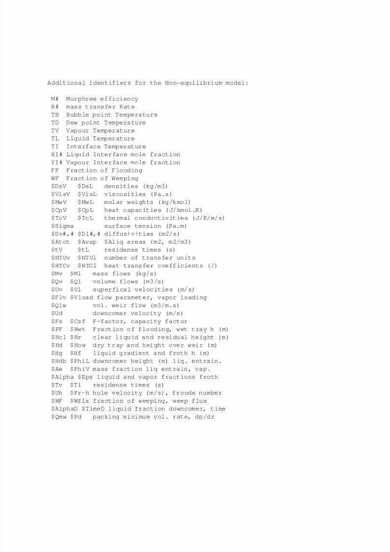
7/27/2019 Chemsep Chemsep HelpHelp
http://slidepdf.com/reader/full/chemsep-chemsep-helphelp 53/59
Additional identifiers for the Non-equilibrium model:
M# Murphree efficiency
R# mass transfer Rate
TB Bubble point Temperature
TD Dew point Temperature
TV Vapour Temperature
TL Liquid Temperature
TI Interface Temperature
XI# Liquid Interface mole fraction
YI# Vapour Interface mole fraction
FF Fraction of Flooding
WF Fraction of Weeping
$DsV $DsL densities (kg/m3)
$VisV $VisL viscosities (Pa.s)$MwV $MwL molar weights (kg/kmol)
$CpV $CpL heat capacities (J/kmol.K)
$TcV $TcL thermal conductivities (J/K/m/s)
$Sigma surface tension (Pa.m)
$Dv#,# $Dl#,# diffusivities (m2/s)
$Atot $Avap $Aliq areas (m2, m2/m3)
$tV $tL residense times (s)
$NTUv $NTUl number of transfer units
$HTCv $HTCl heat transfer coefficients (/)
$Mv $Ml mass flows (kg/s)
$Qv $Ql volume flows (m3/s)
$Uv $Ul superfical velocities (m/s)$Flv $Vload flow parameter, vapor loading
$Qlw vol. weir flow (m3/m.s)
$Ud downcomer velocity (m/s)
$Fs $Csf F-factor, capacity factor
$FF $Hwt Fraction of flooding, wet tray h (m)
$Hcl $Hr clear liquid and residual height (m)
$Hd $How dry tray and height over weir (m)
$Hg $Hf liquid gradient and froth h (m)
$Hdb $PhiL downcomer height (m) liq. entrain.
$Ae $PhiV mass fraction liq entrain, vap.
$Alpha $Eps liquid and vapor fractions froth
$Tv $Tl residense times (s)$Uh $Fr-h hole velocity (m/s), froude number
$WF $Wflx fraction of weeping, weep flux
$AlphaD $TimeD liquid fraction downcomer, time
$Qmw $Pd packing minimum vol. rate, dp/dz

7/27/2019 Chemsep Chemsep HelpHelp
http://slidepdf.com/reader/full/chemsep-chemsep-helphelp 54/59
McCabe-Thiele
McCabe-Thiele diagrams can be displayed by clicking on the Display button on the McCabe-Thiele panel.
The diagram is constructed from the mole fractions of any two components in a multicomponent mixture. The mole fractions
on each axis are normalized so that each axis extends from 0 to 1. ChemSep automatically chooses the two components to be
used in the modified McCabe-Thiele diagram by searching for the two components whose average K-values are closest to,
but either side of unity. The components used in the diagram can be changed if desired. Click on the Auto Select Key comp’s
button for ChemSep to reselect the keys according to this algorithm.
To adapt the diagram click on thr Graph settings checkbox. Two spreadhseets will appear that allow you control over some
aspects of the McCabe-Thiele diagram.
You can change the title that is displayed over the top of the figure on the screen.
ChemSep chooses the two components to be used in the modified McCabe-Thiele diagram by searching for the two compo-
nents whose average K-values are closest to, but on either side of unity. The components used in the diagram can be changed
if desired by clicking on the key-component fields. A list of components will be displayed. Use the cursor control keys and
Enter or the mouse to select one of the components.
It is traditional for a McCabe-Thiele diagram to be displayed with the construction above the 45 degree diagonal that is drawn
across the diagram. It is possible for the construction to appear below the diagonal. Use the ¡i¿Inversion¡/i¿ field in the
McCabe-Thiele spreadsheet to obtain a diagram with the consruction in the desired location. Click on the drop doen list in
the Inversion field to toggle between Yes and No.
The colour, tic spacing, label, and axis titles may be changed from the default settings if desired. It is also possible to change
the range of either axis to zoom in any particularly interesting portion of the diagram. The colour and line style of the stages
lines (the steps of the staircase), the equilibrium line, the operating line, and the Q-lines may be changed. Press Enter with the
cursor on any Lines field to bring up a list of alternatives. Use the cursor keys and Enter to select any of the options displayed.
You can see the result of any changes by clicking on the Display button on the McCabe-Thiele panel at any time.
7/27/2019 Chemsep Chemsep HelpHelp
http://slidepdf.com/reader/full/chemsep-chemsep-helphelp 55/59
Solve Options
This panel is for specifying options related to the simulation programs. As a general rule you should not need to change any
of the default settings but ChemSep provides the flexibility if you require it.
Initialization
Click on the Initialization drop down memu to bring up a list of available options. Click on one of them to select one of these
methods. There are three methods available for initializing the calculations:
Automatic This is the default method because it requires no user supplied estimates of any quantity. Read the technical
information for a discussion of how the initialization is performed for Column simulations.
User supplied you must provide your own initial estimates of the temperatures and/or of the vapour and liquid flows. You
may provide estimates of the temperature profile, the flow profiles, or of both flow and temperature profiles. If yousupply estimates of the flows then you MUST estimate BOTH vapour AND liquid flows. Estimates of temperatures
and flows will be computed automatically if you selected User supplied but forgot to provide any numerical values.
Click on User supplied to bring up a spreadsheet where you may enter your initial guesses.
Previous run uses the results printed in the SEP file. Naturally, this option will not work for an unsolved problem. However,
if the simulation programs fail to find any Old results, they will automatically invoke the Automatic Initialization.
Problems with slightly changed specifications are solved much quicker if previous results are used as starting values
for a new run. You cannot use Previous run if you change the number of stages in a column simulation.
Method
Column and Flash problems are solved using Newton’s method to solve the equations. However, flows, temperatures, andmole fractions are prevented from taking impossible values (i.e. negative values). Technical details of the implementation of
Newton’s method are available here.
Damping
If the straightforward implementation of Newton’s method fails you may want to try damping the corrections that Newton’s
method would otherwise make if left alone. You may specify different damping factors for each of the quantities listed below:
• Flow rates
• Temperatures
• Stream compositions
The adjustments made by the calculation program are mutiplied with the damping factor. Thus, a damping factor of 0.5 causes
the calculations to change the variables only half as much as the algorithm would otherwise change them. Do ¡i¿not¡/i¿ use
damping unless you are sure you need it. The number of iterations will increase.
Accuracy
The accuracy is the value of the norm of the function vector below which calculations are considered converged. In view of
the fact that SI units are used in columns and flash calculations, the default value of the convergence tolerance is 0.000001.
7/27/2019 Chemsep Chemsep HelpHelp
http://slidepdf.com/reader/full/chemsep-chemsep-helphelp 56/59
You may wish to change this in certain cases to obtain better results for mass and heat balance. ChemSep may provide a
warning if you specify a value larger than this but will not prevent you from using any value you choose.
Number of iteratons
The number of iterations fixes the maximum number of iterations allowed before the calculations are terminated. The default
number is 30. This should be more than sufficient for most problems. In the event that the maximum number of iterations
is exceeded, the most recent set of flows, temperatures, and mole fractions will be written to the SEP file. To enter a value
for the convergence tolerance, move the cursor to the accuracy line and type in a new value. The higher the value, the fewer
iterations will be needed but the problem may not be truly converged. If you are not certain if a problem has converged, rerun
it and print the iteration history to a file. Inspection of the flows, temperatures, and compositions will reveal if the problem
has converged or not.
Write History
The central section of the solve options panel is concerned with what you see on the screen or is written to a file by the
simulation programs. The following items can be printed on the screen or to a file:
• Iteration count and sum of squares
• Column profiles (temperature and flows)
• Composition profiles
• Variable and function vectors
• Jacobian matrix
The default responses for all of these items is to print only the iteration count and sum of squares. It is probably not a good
idea to suppress writing of all items otherwise you might not know if the program is working. Printing the variable and
function vectors and the Jacobian matrix is provided for development purposes only and should not be used unless you are
very very curious. The Jacobian matrix is printed in block format. The iteration history can be printed to the screen, a file, or
both. You may select the location for the iteration history to be printed by clicking on the Write History field and selecting one
of the options from the list displayed. Note that if you select file you will have very little idea as to how the calculations are
proceeding until the problem has been solved (or terminates for other reasons). The name of the file to contain the iteration
history should be typed in the History file field. We suggest you use the name of the current SEP file, but use a different
extension: ”.HIS”.
Temporary file
The column simulation program might need to use a file on disk to write information for temporary use only during the
simulation. Specify the name you would like to use for the temporary file in the Temporary file field of the Solve options
spreadsheet. The file is deleted automatically when the simulation is complete.
User Program
ChemSep allows you to run a program other than the simulation prograsm that are part of the program. You may enter the
name of a program that you would like executed in place of these two programs. Enter the full path and extension and any
command line parameters. By default, this field is left empty.

7/27/2019 Chemsep Chemsep HelpHelp
http://slidepdf.com/reader/full/chemsep-chemsep-helphelp 57/59
DOS Extender
Personal computers can operate in two different modes: Protected mode and Real mode. Protected mode programs requirea DOS extender. Protected mode versions of the simulation programs are available for four commercially available DOS
extenders: Rational, Phar Lap, Ergo, and CauseWay. Click on the DOS Extender field and press Enter to bring up a list from
which you can select the DOS Extender.

7/27/2019 Chemsep Chemsep HelpHelp
http://slidepdf.com/reader/full/chemsep-chemsep-helphelp 58/59
Interface Settings
Click on Interface Settings to bring up a new window that allows certain key items to be set.
Input:
Delete trailing zeroes: Click in the checkbox to have ChemSep hide trailing zeroes in input fields (default is not checked).
Always E-notation: Click in the checkbox to force ChemSep to use exponential notation in the display of numbers.
Number of significant digits: Enter a number in the input box besides this text string.
Automatic checking of input: Click in the checkbox to force ChemSep to check input for consistencty (as best as it can
anyway). Default is checked.
Acknowledge unit conversion: Click in the checkbox to force ChemSep to tell you whenever it converts input data to units
that differ from those you specified in the input string. Default is checked, but experienced users will want to uncheck this
option as it gets quite irritating after a while.
Hints:
Show: Click in the checkbox to force ChemSep to show hints.
Delay time: Enter a number in the input box besides this text string. This is the number of seconds that the cursor must be
stationary before a hint will be displayed. The name of the file containing the hints is shown in the file box. You can adapt
this file or make your own hints file.
Components:
Write as text in sep file: Click in the checkbox to force ChemSep to write all property data as text in the sep file (Default is
unchecked).
Default ID: ChemSep can identify components by their formula, structural formula, or their name. Click on the drop down
list to select the preferred style. Default is name.
Synonyms: If the PCD file is searched by component name it may not find the component you are looking for if you entered
part of one of the components synonyms. Most common synonyms are recorded in files with a SYN extension. To enable
ChemSep to search the SYN file for possible components matching the search criterion (name or name fragment), turn on the
Synonym search by specifying the SYN file in the Synonyms File item in the interface window. Click on the browse button
to bring up a directory of SYN files.
File:
Viewer: Displays the name of the program used to view files. ChemSep comes with a public domain file viewer called
lister.exe. To change the name of the file viewer click on the browse button to bring up a directory window.
Editor: Displays the name of the program used to edit files. Default is notepad.exe. To change the name of the editor click
on the browse button to bring up a directory window.

7/27/2019 Chemsep Chemsep HelpHelp
http://slidepdf.com/reader/full/chemsep-chemsep-helphelp 59/59
Technical Background
Process Modelling
Four Properties of Gases and Liquids - a thermodynamic primer
Property Models - a catalog of models in ChemSep
Numerical Solution of Systems of Equations
Flash Calculations
Equilibrium Stage Simulation
Nonequilibrium column modelling
Design Models for Distillation
Design Models for Extraction
Dynamic Models
More information
You can obtain updates to ChemSep Lite from our web site: www.chemsep.com. Read and/or download the latest technical
reference material. ChemSep Case Stories are also available for download.