Chemotaxis and Migration Tool 2

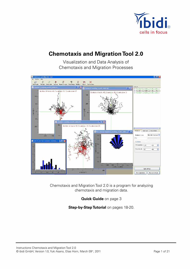
Instructions Chemotaxis and Migration Tool 2.0 © ibidi GmbH, Version 1.0, Yuki Asano, Elias Horn, March 09th, 2011 of 21

Chemotaxis and Migration Tool 2.0 Visualization and Data Analysis of

Chemotaxis and Migration Processes

Chemotaxis and Migration Tool 2.0 is a program for analyzing chemotaxis and migration data.

Quick Guide on page 3

Step-by-Step Tutorial on pages 18-20.


Table of Contents 1 Requirements.................................................................................................................... 3 2 Installation ......................................................................................................................... 3 3 Quick Guide ....................................................................................................................... 3 4 Main Panel......................................................................................................................... 4

4.1 Import Data ................................................................................................................ 4 4.2 Plot Data..................................................................................................................... 6 4.3 Sector Plots................................................................................................................ 6 4.4 Diagrams .................................................................................................................... 7 4.5 Measured Values ........................................................................................................ 9 4.6 Plot Settings ............................................................................................................. 10 4.7 Statistics................................................................................................................... 11

5 Side Panel........................................................................................................................ 11 5.1 Initialization............................................................................................................... 11 5.2 Restrictions .............................................................................................................. 12 5.3 Data Rotation ........................................................................................................... 13

6 Definitions ....................................................................................................................... 14 6.1 Directness [ref. 2] ..................................................................................................... 15 6.2 Center of Mass......................................................................................................... 15 6.3 FMI (Forward Migration Index) [ref. 3]...................................................................... 16 6.4 Rayleigh Test [ref. 4].................................................................................................. 17

7 Step-by-Step Tutorial ........................................................................................................ 18 8 References ...................................................................................................................... 21


1 Requirements • Computer (at least 1 GB RAM) • Windows Platforms XP (or higher) or Linux

2 Installation • Windows: Download ChemotaxisAndMigrationTool.zip to

your computer, unzip, and start Release\Chemotaxis.exe. No further installation is required.

• Linux: Compile the source code to the target system.

3 Quick Guide 1) Import a data table into the program, e.g. from “Manual Tracking” (.xls file) 2) Select the required number of slices (e.g. the number of pictures used for

tracking). The number of slices can be found in your original data table (“Show original data”).

3) Calibrate the software by setting the x/y pixel size and the time interval. The x/y calibration represents the edge length of a pixel in µm. The time interval repre-sents the time between each slice.

4) Press “Apply settings”, after changing the values and parameters. 5) Plot trajectories and export as image. 6) Export the values of FMI, center of mass, velocity, and Rayleigh test from the

“Measured values” window.


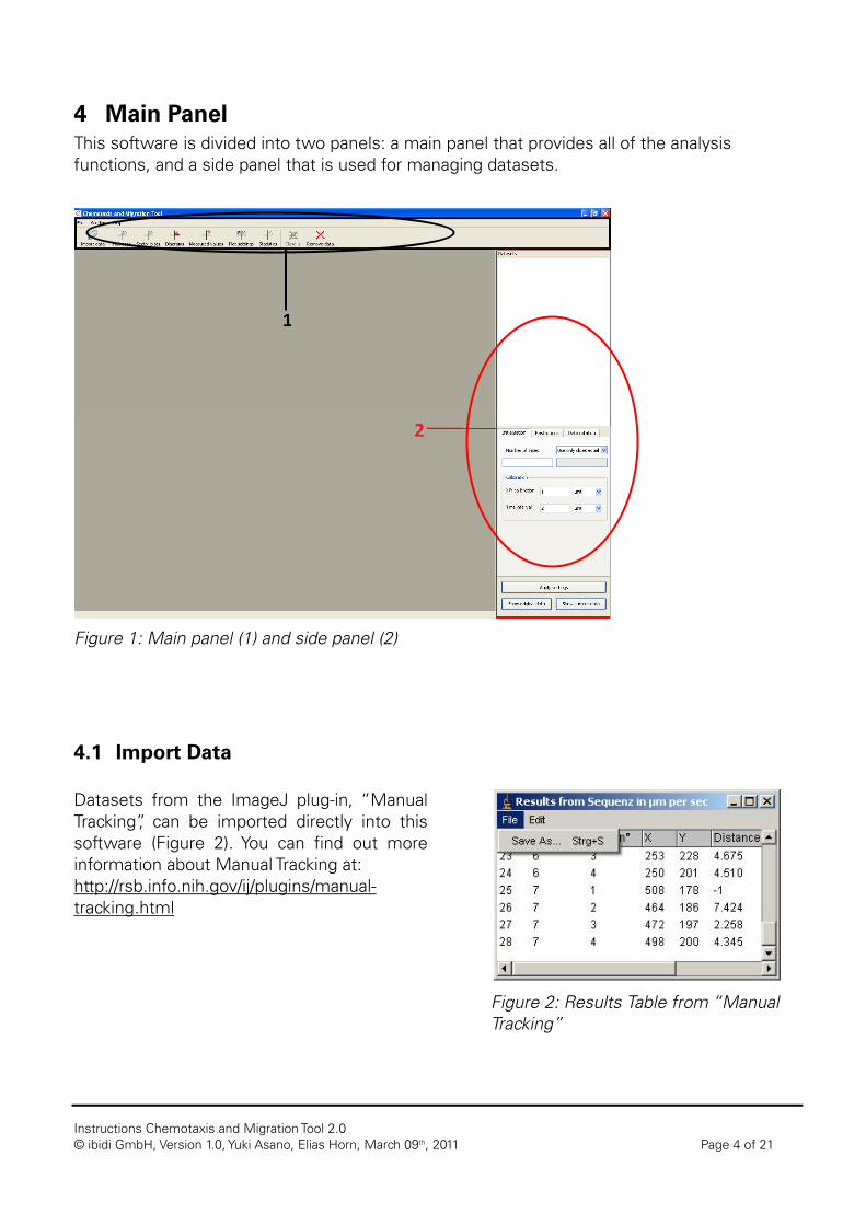
4 Main Panel This software is divided into two panels: a main panel that provides all of the analysis functions, and a side panel that is used for managing datasets.

4.1 Import Data Datasets from the ImageJ plug-in, “Manual Tracking”, can be imported directly into this software (Figure 2). You can find out more information about Manual Tracking at: http://rsb.info.nih.gov/ij/plugins/manual-tracking.html

Figure 1: Main panel (1) and side panel (2)

Figure 2: Results Table from “Manual Tracking”


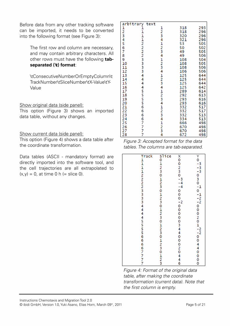
Before data from any other tracking software can be imported, it needs to be converted into the following format (see Figure 3):

The first row and column are necessary, and may contain arbitrary characters. All other rows must have the following tab-separated (\t) format: \tConsecutiveNumberOrEmptyColumn\tTrackNumber\tSliceNumber\tX-Value\tY-Value

Show original data (side panel): This option (Figure 3) shows an imported data table, without any changes. Show current data (side panel): This option (Figure 4) shows a data table after the coordinate transformation. Data tables (ASCII - mandatory format) are directly imported into the software tool, and the cell trajectories are all extrapolated to (x,y) = 0, at time 0 h (= slice 0).

Figure 3: Accepted format for the data tables. The columns are tab-separated.

Figure 4: Format of the original data table, after making the coordinate transformation (current data). Note that the first column is empty.


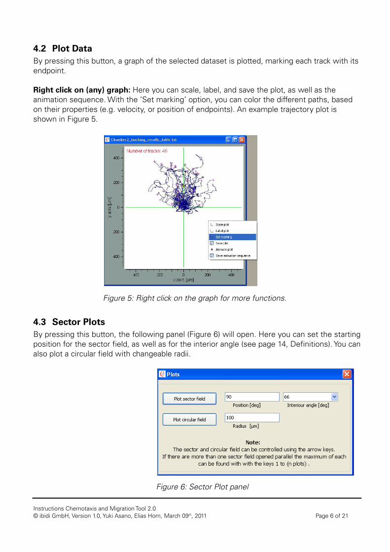
4.2 Plot Data By pressing this button, a graph of the selected dataset is plotted, marking each track with its endpoint. Right click on (any) graph: Here you can scale, label, and save the plot, as well as the animation sequence. With the ‘Set marking’ option, you can color the different paths, based on their properties (e.g. velocity, or position of endpoints). An example trajectory plot is shown in Figure 5.

4.3 Sector Plots By pressing this button, the following panel (Figure 6) will open. Here you can set the starting position for the sector field, as well as for the interior angle (see page 14, Definitions). You can also plot a circular field with changeable radii.

Figure 5: Right click on the graph for more functions.

Figure 6: Sector Plot panel


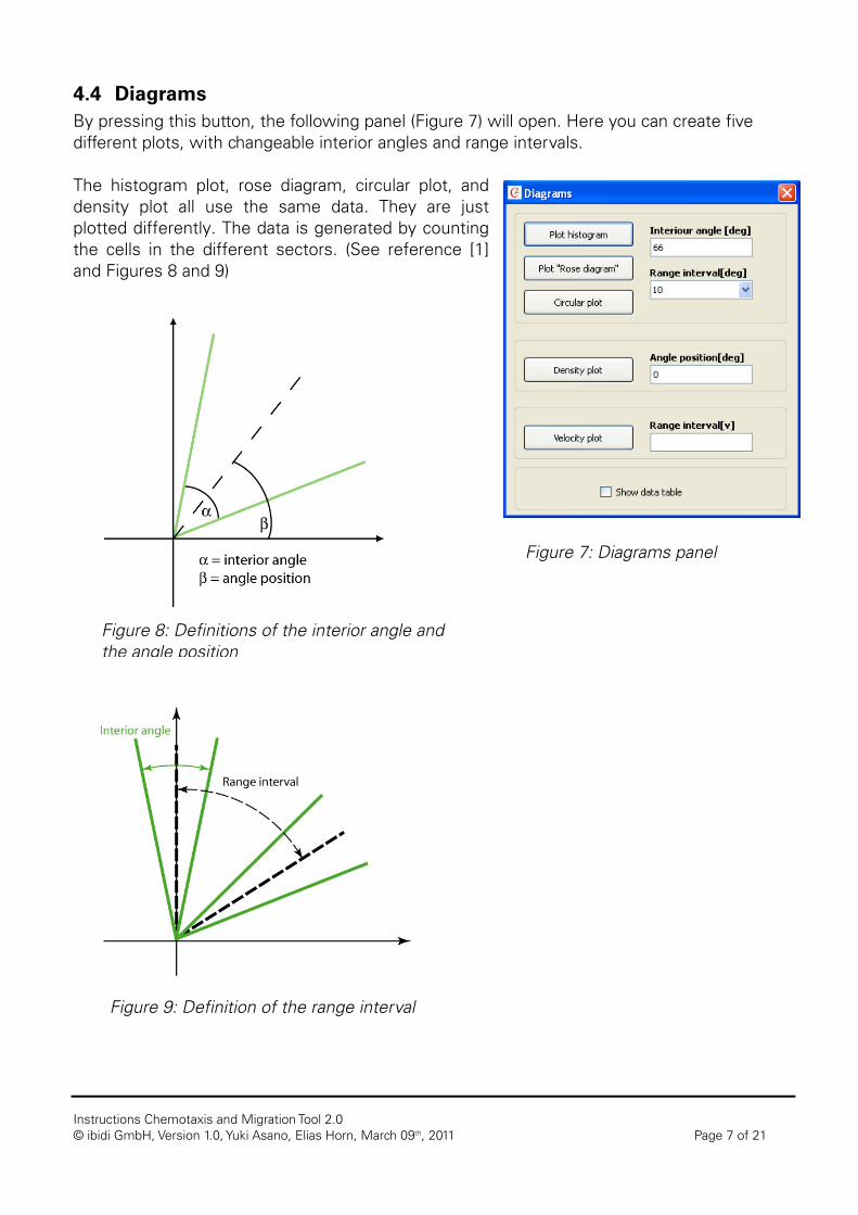
4.4 Diagrams By pressing this button, the following panel (Figure 7) will open. Here you can create five different plots, with changeable interior angles and range intervals. The histogram plot, rose diagram, circular plot, and density plot all use the same data. They are just plotted differently. The data is generated by counting the cells in the different sectors. (See reference [1] and Figures 8 and 9)

Figure 7: Diagrams panel

Figure 8: Definitions of the interior angle and the angle position

Figure 9: Definition of the range interval


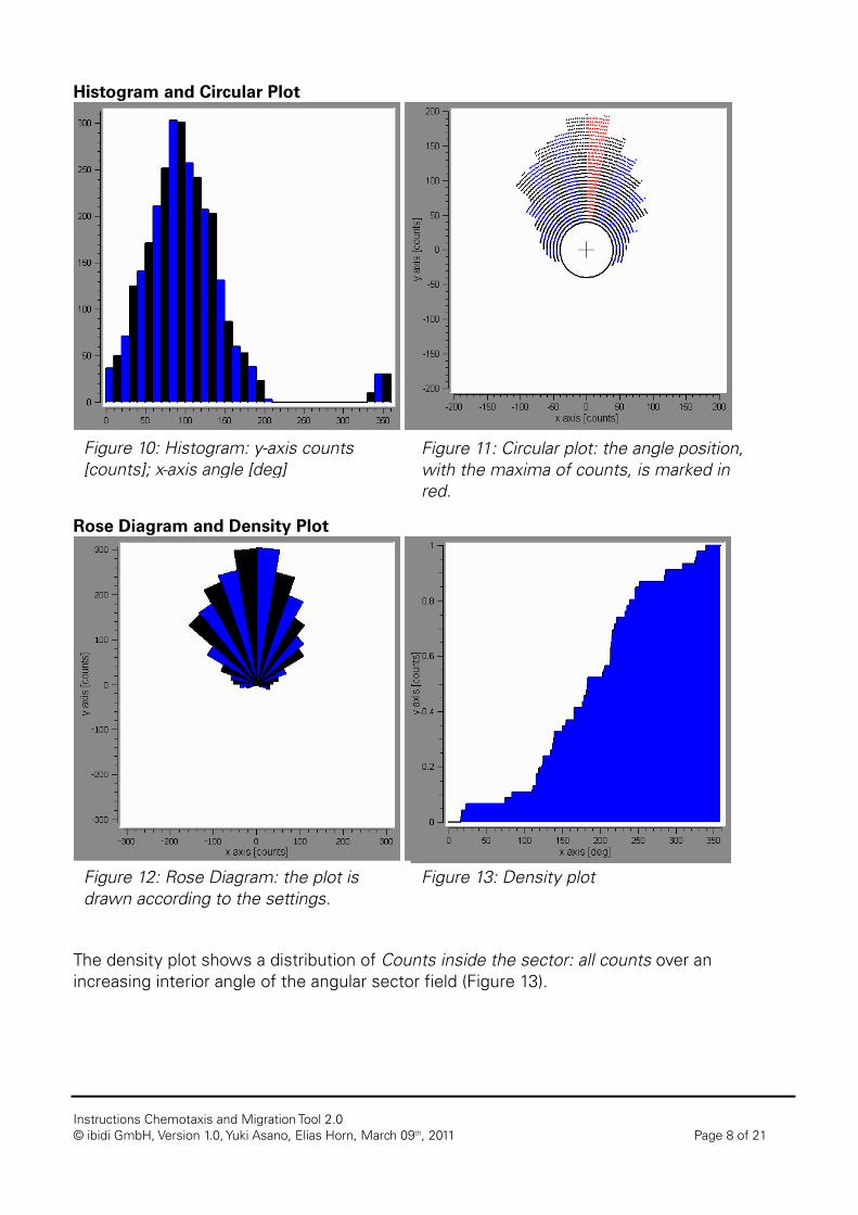
Histogram and Circular Plot

Rose Diagram and Density Plot

The density plot shows a distribution of Counts inside the sector: all counts over an increasing interior angle of the angular sector field (Figure 13).

Figure 11: Circular plot: the angle position, with the maxima of counts, is marked in red.

Figure 10: Histogram: y-axis counts [counts]; x-axis angle [deg]

Figure 12: Rose Diagram: the plot is drawn according to the settings.

Figure 13: Density plot


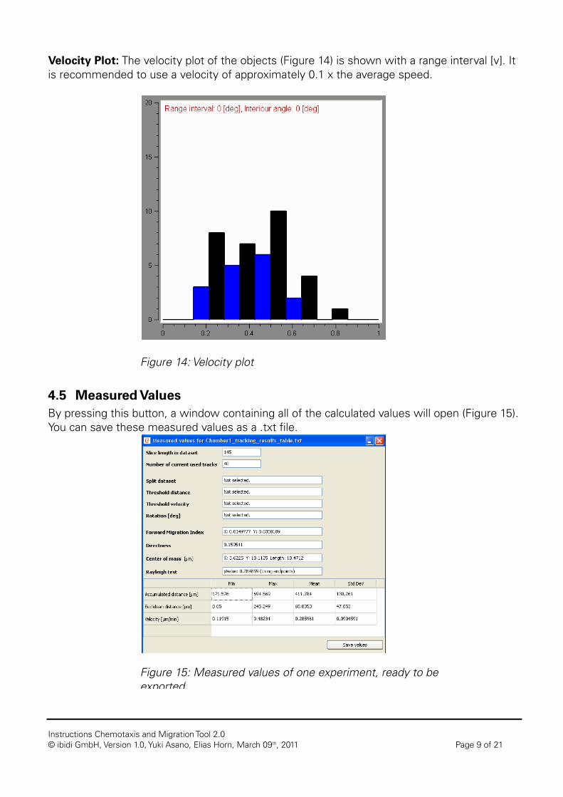
Velocity Plot: The velocity plot of the objects (Figure 14) is shown with a range interval [v]. It is recommended to use a velocity of approximately 0.1 x the average speed.

4.5 Measured Values By pressing this button, a window containing all of the calculated values will open (Figure 15). You can save these measured values as a .txt file.

Figure 14: Velocity plot

Figure 15: Measured values of one experiment, ready to be exported


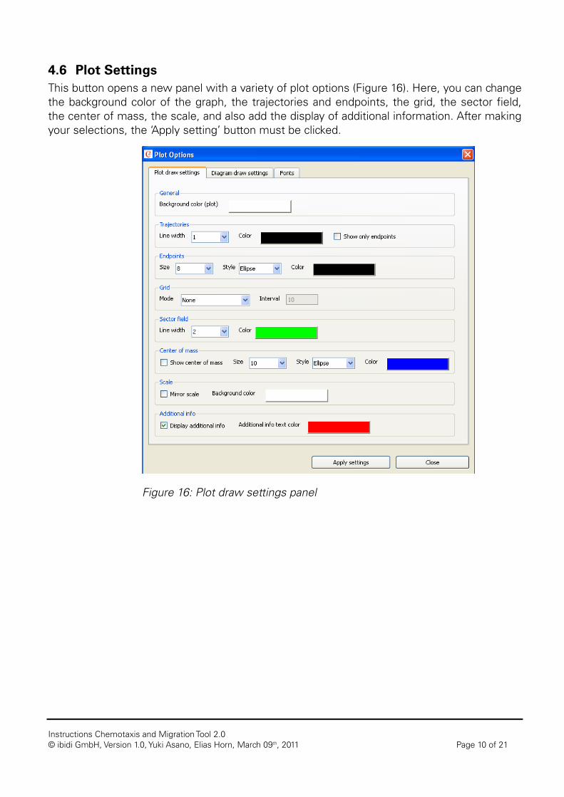
4.6 Plot Settings This button opens a new panel with a variety of plot options (Figure 16). Here, you can change the background color of the graph, the trajectories and endpoints, the grid, the sector field, the center of mass, the scale, and also add the display of additional information. After making your selections, the ‘Apply setting’ button must be clicked.

Figure 16: Plot draw settings panel


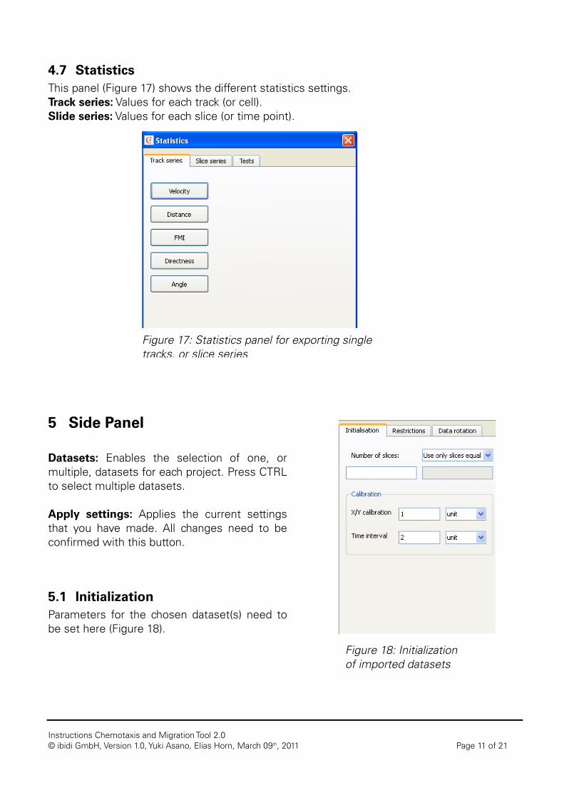
4.7 Statistics This panel (Figure 17) shows the different statistics settings. Track series: Values for each track (or cell). Slide series: Values for each slice (or time point).

5 Side Panel Datasets: Enables the selection of one, or multiple, datasets for each project. Press CTRL to select multiple datasets. Apply settings: Applies the current settings that you have made. All changes need to be confirmed with this button.

5.1 Initialization Parameters for the chosen dataset(s) need to be set here (Figure 18).

Figure 17: Statistics panel for exporting singletracks, or slice series

Figure 18: Initialization of imported datasets


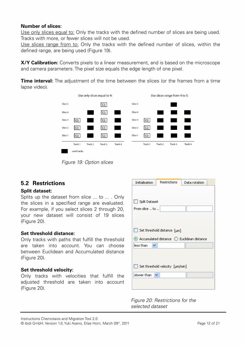
Number of slices: Use only slices equal to: Only the tracks with the defined number of slices are being used. Tracks with more, or fewer slices will not be used. Use slices range from to: Only the tracks with the defined number of slices, within the defined range, are being used (Figure 19). X/Y Calibration: Converts pixels to a linear measurement, and is based on the microscope and camera parameters. The pixel size equals the edge length of one pixel. Time interval: The adjustment of the time between the slices (or the frames from a time lapse video).

5.2 Restrictions Split dataset: Splits up the dataset from slice ... to ... . Only the slices in a specified range are evaluated. For example, if you select slices 2 through 20, your new dataset will consist of 19 slices (Figure 20). Set threshold distance: Only tracks with paths that fulfill the threshold are taken into account. You can choose between Euclidean and Accumulated distance (Figure 20). Set threshold velocity: Only tracks with velocities that fulfill the adjusted threshold are taken into account (Figure 20).

Figure 19: Option slices

Figure 20: Restrictions for the selected dataset


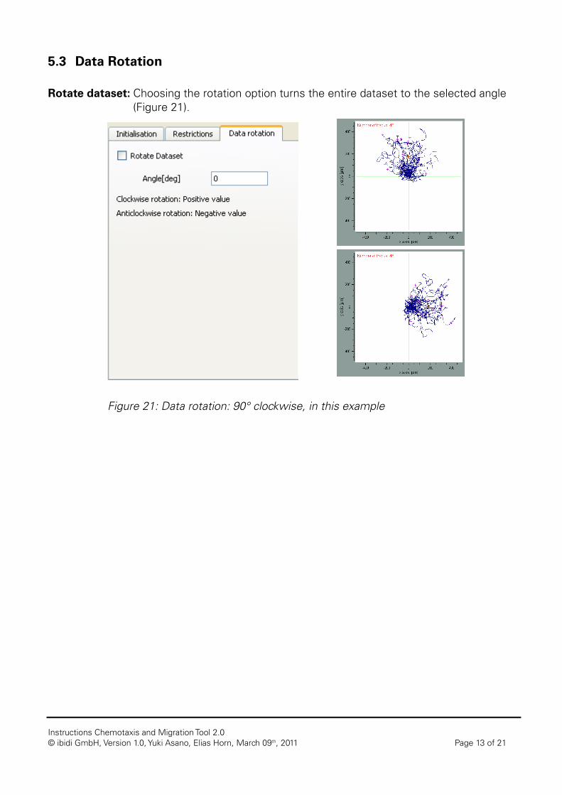
5.3 Data Rotation Rotate dataset: Choosing the rotation option turns the entire dataset to the selected angle

(Figure 21).

Figure 21: Data rotation: 90° clockwise, in this example


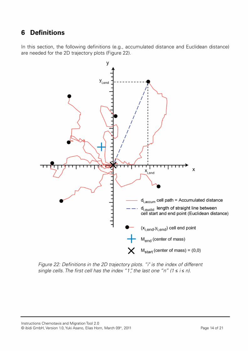
6 Definitions In this section, the following definitions (e.g., accumulated distance and Euclidean distance) are needed for the 2D trajectory plots (Figure 22).

Figure 22: Definitions in the 2D trajectory plots. “i" is the index of different single cells. The first cell has the index “1”, the last one “n” (1 ≤ i ≤ n).


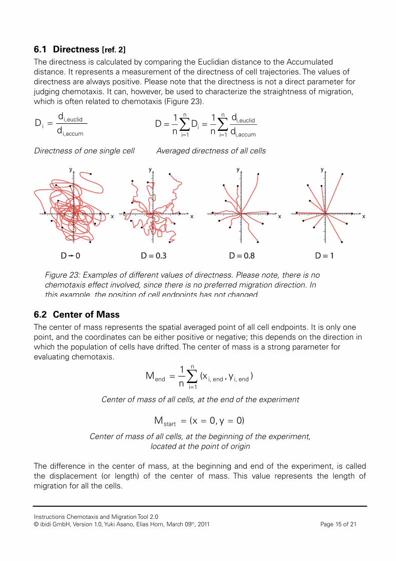
6.1 Directness [ref. 2] The directness is calculated by comparing the Euclidian distance to the Accumulated distance. It represents a measurement of the directness of cell trajectories. The values of directness are always positive. Please note that the directness is not a direct parameter for judging chemotaxis. It can, however, be used to characterize the straightness of migration, which is often related to chemotaxis (Figure 23).

Directness of one single cell Averaged directness of all cells

6.2 Center of Mass The center of mass represents the spatial averaged point of all cell endpoints. It is only one point, and the coordinates can be either positive or negative; this depends on the direction in which the population of cells have drifted. The center of mass is a strong parameter for evaluating chemotaxis.

)y,(xn1

M endi,

n

1iendi,end ∑

=

=

Center of mass of all cells, at the end of the experiment

0)y,0x(Mstart ===

Center of mass of all cells, at the beginning of the experiment, located at the point of origin

The difference in the center of mass, at the beginning and end of the experiment, is called the displacement (or length) of the center of mass. This value represents the length of migration for all the cells.

∑∑==

==n

1i accum,i

euclid,in

1ii d

dn1

Dn1

Daccum,i

euclid,ii d

dD =

Figure 23: Examples of different values of directness. Please note, there is no chemotaxis effect involved, since there is no preferred migration direction. In this example, the position of cell endpoints has not changed.


6.3 FMI (Forward Migration Index) [ref. 3] There are two forward migration indices, which represent the efficiency of the forward migration of cells, and how they relate to the direction of both axes. Both FMI values can be either positive or negative, depending on the direction in which the cell population has drifted. FMI values only make sense when a chemotaxis effect is expected under the following condition: they can be parallel to, or perpendicular to, the x and y axes, but not in 45° angles.

Forward migration indices for all cells Instead of using xFMI and yFMI, it is recommended to define a parallel and perpendicular direction, relative to the gradient. These renamed values, FMI║ (forward migration index, parallel to the gradient) and FMI┴ (forward migration index, perpendicular to the gradient), are advantageous, because they intrinsically define the location of a potential chemoattractant, even without defining the axis. Strong chemotaxis effects are characterized by a high FMI║ (a positive or negative value) and a FMI┴ that is close to “0”. Control experiments, without any chemoattractant, or with homogeneous chemoattractant concentrations, result in values close to “0” for both Forward Migration Indices.

∑=

=n

1i accum,i

end,iFMI d

y

n1

y

∑=

=n

1i accum,i

end,iFMI d

x

n1

x

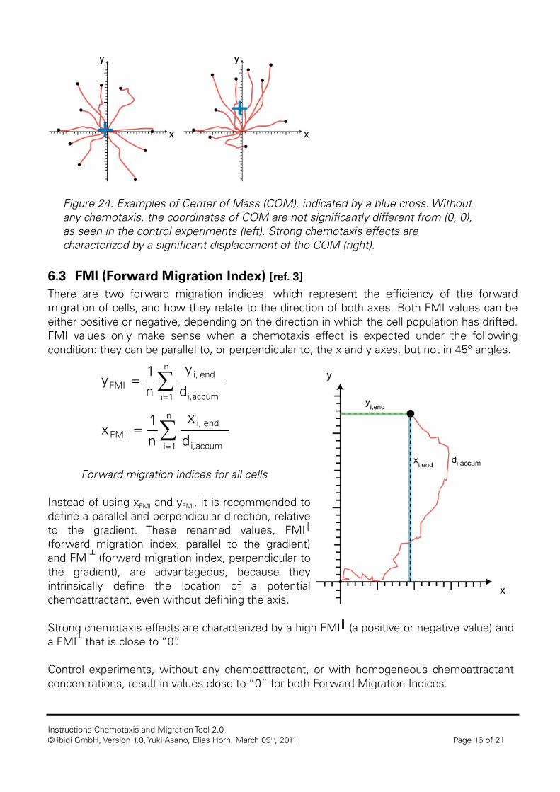
Figure 24: Examples of Center of Mass (COM), indicated by a blue cross. Without any chemotaxis, the coordinates of COM are not significantly different from (0, 0), as seen in the control experiments (left). Strong chemotaxis effects are characterized by a significant displacement of the COM (right).


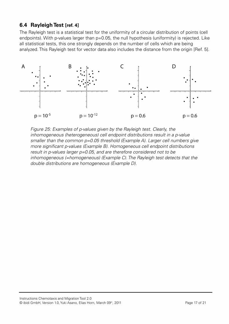
6.4 Rayleigh Test [ref. 4] The Rayleigh test is a statistical test for the uniformity of a circular distribution of points (cell endpoints). With p-values larger than p=0.05, the null hypothesis (uniformity) is rejected. Like all statistical tests, this one strongly depends on the number of cells which are being analyzed. This Rayleigh test for vector data also includes the distance from the origin [Ref. 5].

Figure 25: Examples of p-values given by the Rayleigh test. Clearly, the inhomogeneous (heterogeneous) cell endpoint distributions result in a p-value smaller than the common p=0.05 threshold (Example A). Larger cell numbers give more significant p-values (Example B). Homogeneous cell endpoint distributions result in p-values larger p=0.05, and are therefore considered not to be inhomogeneous (=homogeneous) (Example C). The Rayleigh test detects that the double distributions are homogeneous (Example D).


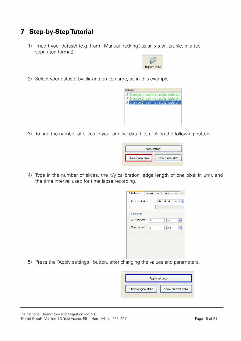
7 Step-by-Step Tutorial

1) Import your dataset (e.g. from “Manual Tracking”, as an xls or .txt file, in a tab-separated format).

2) Select your dataset by clicking on its name, as in this example:

3) To find the number of slices in your original data file, click on the following button:

4) Type in the number of slices, the x/y calibration (edge length of one pixel in µm), and the time interval used for time lapse recording.

5) Press the “Apply settings” button, after changing the values and parameters.


6) Press the “Plot data” button to get to the main plot.

7) You will get a plot that looks similar to this one:

8) By right-clicking on the graph, you can change its appearance (e.g., scale, label, marking), and save the image or its animation.

9) By pressing the “Animate plot” button, you can see the animation.


10) Press the “Measured values” button to see the measured values (see page 14, Definitions).

11) Next, the following window will open and you can save the values by pressing the “Save values” button.

12) By pressing the “Close all” button, you’ll close all windows.


8 References

[1] Mardia Kanti V., Jupp Peter E., 1999, Directional Statistics, Wiley Series

[2] Semmling V., Lukacs-Kornek V., Thaiss C. A., Quast T., Hochheiser K., Panzer U., Rossjohn J., Perlmutter P., Cao J. and Godfrey D. I.; 2010, Alternative cross-priming through CCL17-CCR4-mediated attraction of CTLs toward NKT cell–licensed DCs. Nature Immunology, 10.1038/ni.1848

[3] Foxman Ellen F., Kunkel Eric J., Butcher Eugene C., 1999, Integrating Conflicting Chemotactic Signals: The Role of Memory in Leukocyte Navigation, The Journal of Cell Biology, Volume 147, 577-587

[4] N.I. Fisher, 1993, Statistical analysis of circular data

[5] Moore BR., 1980, A modification of the Rayleigh test for vector data, Biometrika, Volume 67, 175-180

For questions or suggestions, please contact [email protected].

Chemotaxis and Migration Tool 2

Documents

Transcript of Chemotaxis and Migration Tool 2