Chemistry data assimilation validation using independent ...€¦ · Chemistry data assimilation...

Chemistry data assimilation validation using independentobservations

Angela Benedetti1, Richard Engelen1, Johannes Flemming1, HaraldFlentje2, Nicolas Huneeus3, Antje Inness1, Luke Jones1, Eleni Katragkou4,

Julia Marshall 5, Jean-Jacques Morcrette1, Carlos Ordonez6,and Michael Schulz3

(1) ECMWF, Shinfield Park, ReadingRG2 9AX, United Kingdom

Corresponding author: [email protected](2) Deutscher Wetterdienst (DWD)

Meteorologisches Observatorium Hohenpeienberg (FEHp)82383 Hohenpeissenberg, Germany

(3) Laboratoire des Sciences du Climat et de lEnvironnement91191 Gif-sur-Yvette Cedex, France

(4) National Kapodistrian University of Athens - AristotleUniversity of ThessalonikiAthens, Greece

(5) Max-Planck-Institut fur Biogeochemie07745 Jena, Germany

(6) UK Met Office,Exeter, United Kingdom

ABSTRACT

An analysis system for greenhouse gases, reactive gases andaerosols has been developed at the European Centrefor Medium–Range Weather Forecasts, under the Global and regional Earth-system Monitoring using Satellite andin-situ data (GEMS) project. The GEMS modelling and analysis systems are fully integrated in the operationalfour–dimensional assimilation system. Their purpose is toproduce global forecasts and reanalyses of atmosphericcomposition using satellite data. A multi–year reanalysishas been conducted for 2003-2007. Analysed fieldsinclude carbon dioxide, methane, carbon monoxide, ozone, formaldehyde, nitrogen oxides and aerosol opticaldepth. These fields are being evaluated using independent observations. This study presents a collection of resultsfrom the validation activities performed both by ECMWF and by various European institutes, which were part ofthe GEMS consortium.

1 Introduction: the GEMS and MACC projects

The Global and regional Earth-system Monitoring using Satellite and in-situ data (GEMS) project whichfinished in May 2009 included thirty-two European partners with expertise in various aspects of atmo-spheric composition monitoring. GEMS was part of the GlobalMonitoring for Environment and Se-curity (GMES) initiative and was established under European Commission funding in 2005 to createan assimilation and forecasting system for monitoring aerosols, greenhouse gases and reactive gases, atglobal and regional scales, through exploitation of satellite and in–situ data (Hollingsworth et al., 2008).An important component of GEMS has been the forecasting of regional air quality at the European scale.This is performed with an ensemble of air quality models fromthe participating institutes. Boundaryconditions for the high–resolution models are provided by the global model.

ECMWF Workshop on Diagnostics of Data Assimilation System Performance, 15-17 June 2009 145

BENEDETTI, A. ET AL.: CHEMISTRY DATA ASSIMILATION VALIDATION

The basis for the global GEMS forecast and analysis schemes is the operational ECMWF IntegratedForecasting System (IFS) that includes the incremental four–dimensional variational analysis system.The system has been extended to include new prognostic variables for atmospheric tracers (i.e. gasesand aerosols). A coupled chemical transport model is also part of the GEMS system and providestendencies for the chemically–active species which are present in the model (Flemming et al., 2009).

The follow–up to GEMS is the Monitoring of Atmospheric Composition and Climate (MACC) projectwhose objectives are largely the same as GEMS with a greater emphasis on user–oriented applications.

2 Brief description of the GEMS-ECMWF integrated analysis system

The main characteristics of the integrated GEMS–ECMWF analysis system are:

• T159 ( 120km) horizontal resolution,

• 60 vertical layers; top level at 0.1 hPa,

• model physics based on ECMWF model cycle 32r3,

• Four-dimensional variational (4DVAR) analysis using a 12-hour time window,

• Wavelet-based background error covariances for all tracers, and background error statistics com-puted using the NMC method (Parrish and Derber, 1992).

Control variables for the system include: carbon dioxide, methane, carbon monoxide, ozone, formalde-hyde, nitrogen oxides and total aerosol mass. Specific observational operators have been developed forthe various constituents, taking into consideration the maturity of the observing systems and the avail-ability of observations suitable for assimilation. For example, the analysis of CO2 is driven by AIRSradiance observations, whereas the reactive gases analysis is driven by retrievals of total column inte-grated amounts from various space-borne sensors such as MIPAS, OMI, SCHIAMACHY, SBUV, MLS,GOME, MOPITT. For the aerosol analysis, retrieved aerosol optical depths from the MODIS sensor areused. More details on the three sub-components of the GEMS system can be found inEngelen et al.(2009); Inness et al.(2009); Benedetti et al.(2009).

The GEMS reanalysis of the years 2003-2007 was completed in March 2009. As of July 2009, theGEMS reanalysis has been restarted to cover 2008 and 2009, and it has now reached November 2008.

3 Validation metrics

Although there were no prescribed standards for the validation exercise, for the sake of consistency mostvalidating groups chose common validation metrics as well as similar methods to display results. A fewof the metrics used are listed below

• Modified normalized mean bias,B =( 2

N

)

∑Ni=1

fi−oifi+oi

• Correlation coefficient,r =1N ∑N

i=1 ( fi− f )(oi−o)σ f σo

• Normalized Median Bias,NMedB= Median∑regioni=1

( fi−oi)Median(oi )

For the visualization the following methods were used

146 ECMWF Workshop on Diagnostics of Data Assimilation System Performance, 15-17 June 2009


• Taylor diagrams (standard deviation and correlation)

• Scatterplots (bias and correlation)

• Line plots (time series of bias and Root Mean Square error)

These can be considered to provide quantitative information about the quality of the analysis with respectto the independent observations. Qualitative informationis also displayed using profile/cross sectionplots and maps.

4 Validation of the greenhouse gas analysis

The assimilation system for greenhouse gases include CO2 and methane (CH4) as prognostic variablesand control variables. The observations assimilated consist of AIRS radiances for CO2 and SCHIA-MACHY retrievals for CH4. For the CO2 analysis, the verification observations are ground-based flaskmeasurements and aircraft observations as shown in figure1 while IASI CH4 retrievals, that were notassimilated, constitute the validating dataset for the CH4 analysis.

Figure 1: Map of observations for validating analysed CO2.

4.1 Verification of the CO2 analysis

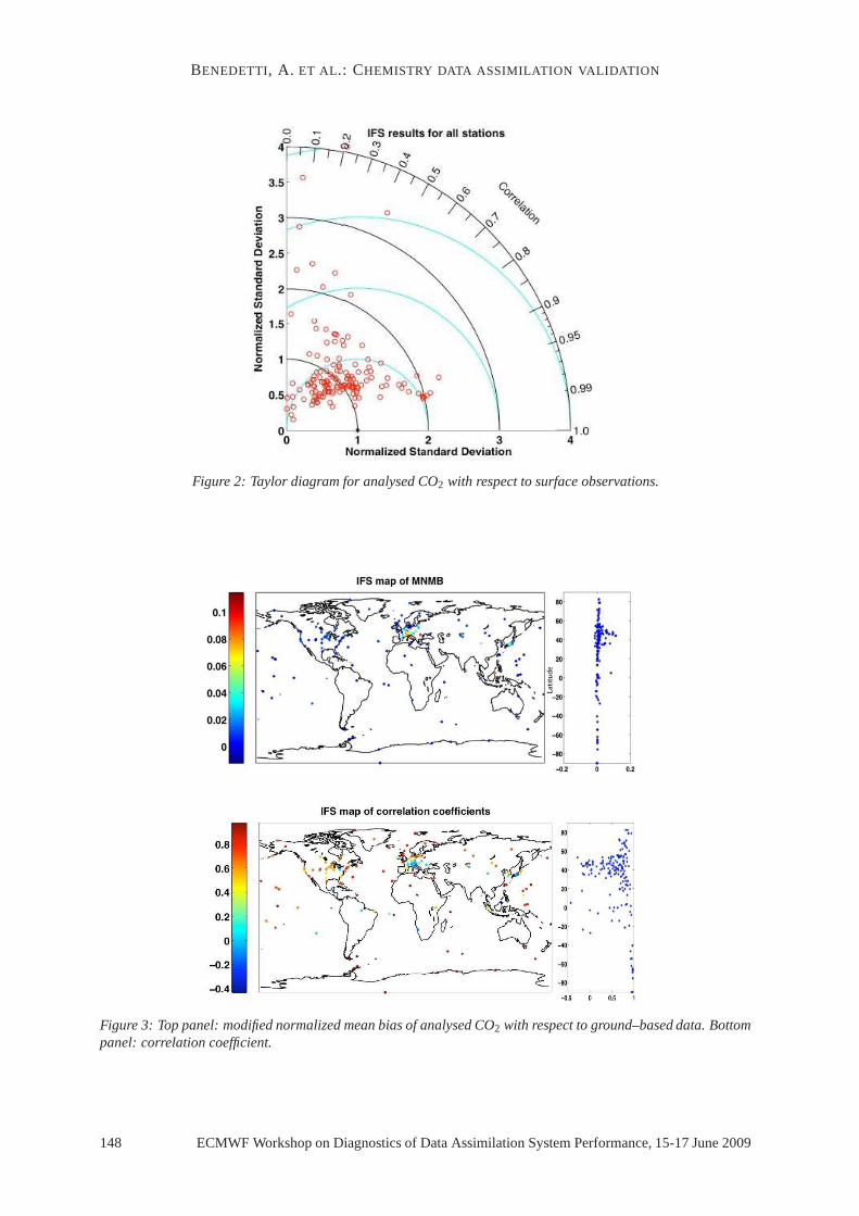
Four-dimensional analysed CO2 fields were sub-sampled to match available surface, tower, ship-based,and flight data The resultant time series were compared to available observations. Statistical results weresummarized by means of a Taylor diagram (figure2), and by using maps of modified mean normalizedbias and correlation coefficient (figure3).

The performance of the CO2 analysis is detailed in the Taylor diagram of figure2 which shows onlya few stations for which the standard deviation is large and the correlation is poor. Otherwise moststations crowd around the reference point, indicating a good agreement of the modelled CO2 with theobservations. The Taylor diagram does not show, by construction, the analysis bias which is insteadillustrated in the top panel of figure3. The figure shows that the analysed CO2 has up to a 10% positivebias over Europe. In general, the Southern Hemisphere is well-constrained, while a slightly positivetendency can be seen in the Northern Hemisphere. This seems related to a seasonal cycle which is tooweak. The bottom panel of the same figure shows a map of the correlation coefficient. Remote stationsshow good agreement while poor correlation are seen over highly populated regions with heterogeneousfluxes such as Europe.



Figure 2: Taylor diagram for analysed CO2 with respect to surface observations.

Figure 3: Top panel: modified normalized mean bias of analysed CO2 with respect to ground–based data. Bottompanel: correlation coefficient.



4.1.1 Comparison with CO2 observations from the Mauna Loa observatory

Figure4 shows the performance of the analysis in comparison with observations of CO2 surface concen-tration taken at the Carbon Cycle In Situ Observatory of Mauna Loa (19 N, 155W, 3397 m ASL). Theplot (which can easily be considered the most infamous plot of the century) shows the rapid increase ofCO2 over the last decade. The analysis does a good job in reproducing such trend especially in morerecent years, possibly due to general improvements in the observing system (for example the inclusionof GPS radio occultation data) leading to a better CO2 analysis.

Figure 4: Comparisons of CO2 concentration observed at the Mauna Loa observatory (black) with the GEMSanalysis (red).

4.2 Verification of the methane analysis

The analysed methane fields were sub-sampled in time and space to match individual retrievals froman independent satellite The appropriate weighting function was applied (not shown). Monthly meanmaps were compared for spatial and temporal correlation (figure5). Qualitatively, the analysed methanecompares well with IASI retrievals, but tends to be higher onaverage, especially in the Indian Oceanand Indian Sub-continent regions.

Figure 5: Left: methane fields retrieved from IASI observations; Right: methane fields from the GEMS reanalysis.



5 Validation of the aerosol analysis

Aerosol prognostic variables include 3 bins for desert dust, 3 bins for sea-salt, hydrophobic and hy-drophilic organic matter, hydrophobic and hydrophilic black carbon, and sulphate. The control variableis formulated in terms of the total aerosol mixing ratio. Assimilated observations are the MODIS AerosolOptical Depths (AODs) at 550 nm over land and ocean. Observation errors over ocean are prescribedas functions of the satellite scattering angle. Errors overland are assigned as 50% of the optical depthvalue. For more details seeBenedetti et al.(2009).

Validation datasets used are optical depths from AERONET, AEROCE (U. of Miami), and compilationdatasets. These are shown in figure6.

Figure 6: Map of observations for the validation of the aerosol analysis. Optical Depth 550 nm & AngstrmExponent (AERONET) (diamonds); Surface Concentration DD (AEROCE, U. de Miami) (stars, not discussedhere) and Total Deposition by Ginoux et al, 2001 (squares, not discussed). AERONET Stations where a speciesdominates the total optical depth for at least 4 months are marked with the following symbols: black diamonds =desert dust stations; red diamonds = biomass burning stations, green diamonds = sea salt stations.

The verification has focused so far on the AOD at 550 and 865 nm and the Angstrom exponent,α ,defined from the relationshipτ1

τ2=

(λ1λ2

)

−α. A validation effort is currently under way to validate also

the surface concentrations of the aerosol species.

5.1 Observation statistics from the analysis of MODIS data

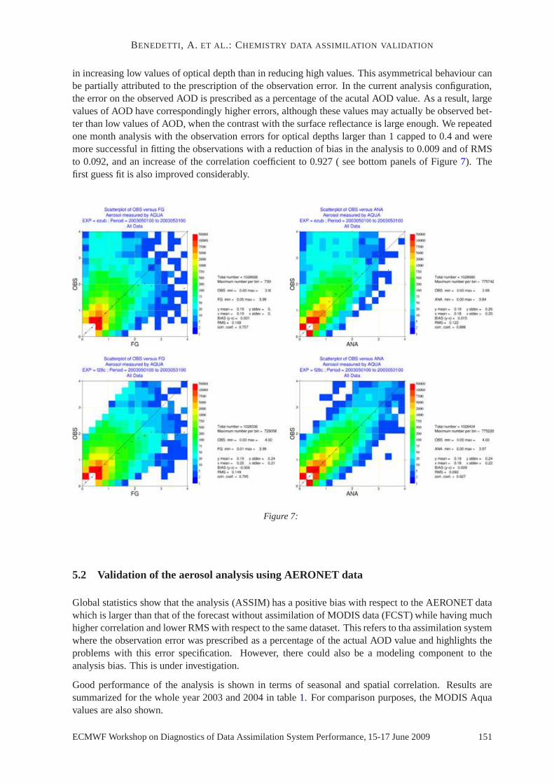
The aerosol optical depth from the analysis for the whole month of May 2003 was used to investigatethe analysis performance with respect to the assimilated observations. In a successful analysis the de-partures should always be smaller than the first guess departures (and the analysis should better matchthe observations, at least in a statistical sense). Figure7 shows scatterplots of assimilated aerosol obser-vations versus first guess (top left) and analysis (top right). By visual inspection, it is apparent that thescatter in the analysis is smaller than in the first guess. Theroot mean square error with respect to theMODIS data is lower for the analysis (0.122) than for the firstguess (0.168) while the correlation coeffi-cient is higher for the analysis (0.888) than for the first guess (0.757), indicating a good performance ofthe analysis. However, while we did not expect the analysis to improve on the first guess biases, it wassurprising to notice that the analysis effectively has a larger bias than the first guess. The distributionappears to be skewed and it is evident from the shape of the scatterplot that the analysis is more efficient



in increasing low values of optical depth than in reducing high values. This asymmetrical behaviour canbe partially attributed to the prescription of the observation error. In the current analysis configuration,the error on the observed AOD is prescribed as a percentage ofthe acutal AOD value. As a result, largevalues of AOD have correspondingly higher errors, althoughthese values may actually be observed bet-ter than low values of AOD, when the contrast with the surfacereflectance is large enough. We repeatedone month analysis with the observation errors for optical depths larger than 1 capped to 0.4 and weremore successful in fitting the observations with a reductionof bias in the analysis to 0.009 and of RMSto 0.092, and an increase of the correlation coefficient to 0.927 ( see bottom panels of Figure7). Thefirst guess fit is also improved considerably.

Figure 7:

5.2 Validation of the aerosol analysis using AERONET data

Global statistics show that the analysis (ASSIM) has a positive bias with respect to the AERONET datawhich is larger than that of the forecast without assimilation of MODIS data (FCST) while having muchhigher correlation and lower RMS with respect to the same dataset. This refers to tha assimilation systemwhere the observation error was prescribed as a percentage of the actual AOD value and highlights theproblems with this error specification. However, there could also be a modeling component to theanalysis bias. This is under investigation.

Good performance of the analysis is shown in terms of seasonal and spatial correlation. Results aresummarized for the whole year 2003 and 2004 in table1. For comparison purposes, the MODIS Aquavalues are also shown.



FCST FCST ASSIM ASSIM MODIS Aqua MODIS Aqua2003 2004 2003 2004 2003 2004

AERONET AOD 0.22 0.22 0.22 0.22 0.22 0.22# N months 1125 1422 1225 1422 1143 1292

AOD 0.24 0.26 0.27 0.27 0.20 0.20Corr 0.68 0.69 0.82 0.82 0.79 0.78RMS 0.13 0.14 0.11 0.12 0.11 0.12

Std Dev 0.76 0.73 0.81 0.79 0.89 0.93Seasonal r 0.75 0.76 0.80 0.80 0.81 0.79Spatial r 0.71 0.73 0.78 0.81 0.80 0.81

Table 1: Global statistical comparison of aerosol free-running forecast and analysis with AERONET data.

Figure8 shows scatterplots and pdfs of optical depth at 865 nm which compare the global AERONETdata with the free-running forecast (no assimilation) and the analysis. The correlation between theobservations and the analysis is greater, but the bias in theanalysis is larger than that of the forecast. Ashighlighted when discussing the analysis fit to the assimilatedassimilated observations (see subsection5.1), the analysis does not seem to be able to correct the large AOD values.

Figure9 shows the Angstrom coefficient for the free-running forecast and the analysis as they comparewith AERONET data. It can be seen that there is no improvementbetween the free–running experimentand the analysis. In general there is an over-estimation of the amount of coarse aerosol and underesti-mation of fine aerosol in the model.

Figure 10 summarizes results with the aid of a Taylor diagram. The free–running forecast withoutassimilation is marked in black, while the analysis is in red. The following fields are plotted: aerosoloptical depth at 550 nm; aerosol optical depth at 865 nm; Angstrom exponent fine mode aerosol opticaldepth at 550 nm; coarse mode aerosol optical depth at 550 nm.

Preliminary conclusions from the comparison with AERONET observations can be drawn as follows:

- Significant improvement in column integrated aerosol variables in terms of correlation and stan-dard deviation.

- A positive bias is present in the analysis.

- Assimilation of AOD at 550 nm improves also AOD at 865 nm which is not assimilated.

- Improvement of AOD at 550 and 865 nm does not translates intoimprovement of Angstromexponent suggesting that assimilation acts on correcting total aerosol burden rather than size dis-tribution.

- Overestimation of the Angstrom exponent for coarse aerosols indicates smaller particles in themodel.

- Too much fine mode sea salt represented in the model (not shown).

- Not enough Desert Dust is emitted and too much fine Desert Dust is transported far off sourceregions in the forecast model (not shown).

5.3 Another independent comparison with AERONET data

Another independent comparison with AERONET data was performed at ECMWF. The aerosol opticaldepth data used in this comparison are the Level 2.0 (cloud-screened and quality-assured) product. The



Figure 8: Optical depth at 865 nm: free-running forecast (left) and analysis (right). AERONET sunphotometerdata are shown in red in the pdf plot; model values are in blue.

Figure 9: Scatterplot of Angstrom coefficient for the free-running forecast (red) and the analysis (blue) comparedwith AERONET data.



Figure 10: Taylor diagram for model AOD and Angstrom coefficient with respecto to AERONET observations.Aerosol optical depth at 550 nm is shown with full circles; aerosol optical depth at 865 nm is shown with crosses;the Angstrom exponent is marked with squares, the fine mode aerosol optical depth at 550 nm with triangles; andthe coarse mode aerosol optical depth at 550 nm is indicated with diamonds.

site selection was thinned using an algorithm which looped through all available sites, checking each forproximity to others. If two sites were found within 700 km of each other, then the site with greater dataavailability (measured as the number of 6 hour periods with at least one observation at 500 nm duringJanuary 2003) was kept and the other discarded. This resulted in a selection of 41 stations shown infigure11.

Figure12shows some comparisons with AERONET independent data for the month of May 2003. TheAODs from the model are averages over 6 hours, whereas the AERONET observations are instantaneous.To make them comparable, the AERONET observations are averaged over the same period. Because theobservations are unevenly spaced in time, a weighted mean iscomputed in such a way that it is equalto the mean of the series of straight lines that join neighbouring observations over the period. ForecastAODs from the free–running experiment and the analysis are bilinearly interpolated to the observationlocation in space.

The analysis is shown in red and the free–running forecast inblue. Both plots show that the analysisis on average closer to the AERONET observations displayinga lower bias (left panel) and RMS error(rigth panel) than the forecast.

From this comparison with AERONET data it appears that the validation outcome is subject to thechoice of the validating dataset (or a subset of). This highlights the fact that the quality of the analysisvaries on a spatial, possibly regional scale, depending on the dominating aerosol species. Althoughin apparent contradiction with the results displayed in table 1, it shows the fact that the global spatialredistribution of AOD operated through the assimilation ofMODIS data into the model was successful.It also emphasizes that global averages, although very useful for a quick assessment of the analysisquality, may hide some important features. The issue of the global analysis bias is, however, still to beaddressed.



Figure 11: Map of the AERONET stations used for the verification of the aerosol analysis performed at ECMWF

-0.5

-0.4

-0.3

-0.2

-0.1

0

0.1

0.2

0.3

0.4

0.5

MAY 20032 3 4 5 6 7 8 9 10 11 12 13 14 15 16 17 18 19 20 21 22 23 24 25 26 27 28 29 30 31

Meaned over 41 sites globally. Period=1-31 May 2003. FC start hrs=00,12Z.FC-OBS Bias. Model AOT at 550nm against L2.0 Aeronet AOT at 500nm.

0

0.05

0.1

0.15

0.2

0.25

0.3

0.35

0.4

0.45

0.5

MAY 20032 3 4 5 6 7 8 9 10 11 12 13 14 15 16 17 18 19 20 21 22 23 24 25 26 27 28 29 30 31

Meaned over 41 sites globally. Period=1-31 May 2003. FC start hrs=00,12Z.

RMS Error. Model AOT at 550nm against L2.0 Aeronet AOT at 500nm.

Figure 12: Bias (left) and RMS (right) of the AOD at 550 nm fromthe free–running forecast (blue) and analysis(red) with respect to AERONET ground–based observations at500 nm for May 2003.



5.4 Case study: Saharan dust outbreak of March 2004

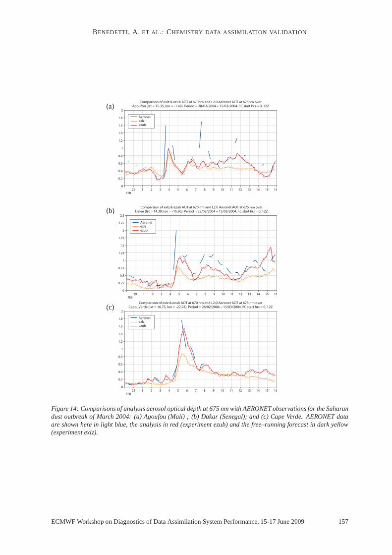
To further assess the performance of the analysis we looked at a case study relative to a major Saharandust storm recorded in early March 2004. The storm was detected by several satellite sensors andground–based sites. Very large values of AOD were recorded.Figure13 shows comparisons betweenAODs from the free-running model and the analysis compared to MODIS observations for 6 March2004. The shape of the dust outflow is well represented in bothfree–running model and analysis, butthe magnitude of the AODs is much larger in the latter in better agreement with the observations. Thisis also confirmed by looking at the AERONET data at three key stations (see Figure14). The peaksshown in the AERONET data are well captured by the analysis, despite the lack of MODIS data overthe in-land desert sites.

Figure 13: 6th March 2004 Saharan dust outbreak: comparisons of free-running model and analysis 550 nm AODswith MODIS (assimilated) observations: (a) free running model ; (b) analysis ; and (c) MODIS observations.

5.5 Vertical profiles comparison using CALIPSO data

Data from CALIPSO were used to qualitatively assess the vertical distribution of the aerosol in the anal-ysis. Generally, a good agreement is achieved on the vertical (see figure15) but there is no improvementwith respect to a forecast without assimilation of AOD observations. This is not unexpected since theAOD observations cannot constrain the vertical profile of extinction but only the model total opticaldepth.

It appears that too much aerosol is present in the upper troposphere in the analysis. This is likelyto depend on interaction between convection/vertical diffusion and the aerosol transport. We plan tocompare extinction profiles and obtain more quantitative profile information.

6 Validation of the reactive gas analysis

The reactive gases included in the GEMS analysis are ozone (O3), carbon monoxide (CO), nitrogenoxides (NOx), and Formaldehyde. The chemical model MOZART is coupled with IFS which providesthe meteorological forcing to the CTM (Flemming et al., 2009). Chemical tendencies are provided toIFS every hour.

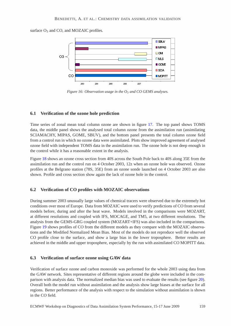
Observations used for ozone and carbon monoxide are shown infigure 16 along with the timeline ofusage.

The verifying observations for the reactive gases analysisare provided by TOMS, SCHIAMACHY,GAW



(a)

(b)

(c)

Figure 14: Comparisons of analysis aerosol optical depth at675 nm with AERONET observations for the Saharandust outbreak of March 2004: (a) Agoufou (Mali) ; (b) Dakar (Senegal); and (c) Cape Verde. AERONET dataare shown here in light blue, the analysis in red (experimentezub) and the free–running forecast in dark yellow(experiment exlz).



Figure 15: Qualitative comparison of aerosol occurence from the CALIPSO lidar (top panel) with the analysisfields from the GEMS reanalysis (bottom panel).



surface O3 and CO, and MOZAIC profiles.

Figure 16: Observation usage in the O3 and CO GEMS analyses.

6.1 Verification of the ozone hole prediction

Time series of zonal mean total column ozone are shown in figure 17. The top panel shows TOMSdata, the middle panel shows the analysed total column ozonefrom the assimilation run (assimilatingSCIAMACHY, MIPAS, GOME, SBUV), and the bottom panel presents the total column ozone fieldfrom a control run in which no ozone data were assimilated. Plots show improved agreement of analysedozone field with independent TOMS data in the assimilation run. The ozone hole is not deep enough inthe control while it has a reasonable extent in the analysis.

Figure18shows an ozone cross section from 40S across the South Pole back to 40S along 35E from theassimilation run and the control run on 4 October 2003, 12z when an ozone hole was observed. Ozoneprofiles at the Belgrano station (78S, 35E) from an ozone sonde launched on 4 October 2003 are alsoshown. Profile and cross section show again the lack of ozone hole in the control.

6.2 Verification of CO profiles with MOZAIC observations

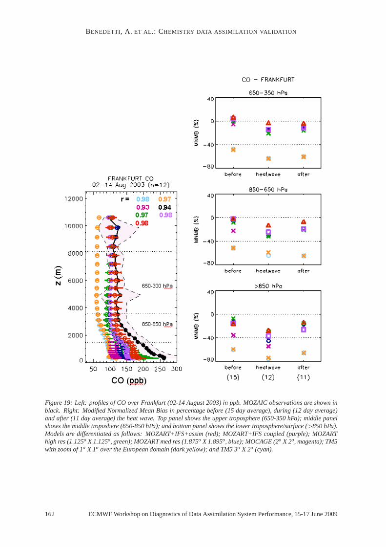
During summer 2003 unusually large values of chemical tracers were observed due to the extremely hotconditions over most of Europe. Data from MOZAIC were used toverify predictions of CO from severalmodels before, during and after the heat wave. Models involved in the comparisons were MOZART,at different resolutions and coupled with IFS, MOCAGE, and TM5, at two different resolutions. Theanalysis from the GEMS-GRG coupled system (MOZART+IFS) wasalso included in the comparisons.Figure19 shows profiles of CO from the different models as they comparewith the MOZAIC observa-tions and the Modified Normalized Mean Bias. Most of the models do not reproduce well the observedCO profile close to the surface, and show a large bias in the lower troposphere. Better results areachieved in the middle and upper troposphere, especially bythe run with assimilated CO MOPITT data.

6.3 Verification of surface ozone using GAW data

Verification of surface ozone and carbon monoxide was performed for the whole 2003 using data fromthe GAW network. Sites representative of different regionsaround the globe were included in the com-parison with analysis data. The normalized median bias was used to evaluate the results (see figure20).Overall both the model run without assimilation and the analysis show large biases at the surface for allregions. Better performance of the analysis with respect tothe simulation without assimilation is shownin the CO field.



Figure 17: Time series of zonal mean total column ozone in Dobson units. Top panel: TOMS data; middle panel:analysed total column ozone; and bottom panel: total columnozone field from a control run.



Figure 18: Ozone cross section from 40S across the South Poleback to 40S along 35E from assimilation run (top)and control run (bottom) on 4 October 2003, 12z. Ozone profiles at the Belgrano station (78S, 35E) from an ozonesonde launched on 4 October 2003 (black), assimilation run (red) and control (green). The Unit is mPa.



Figure 19: Left: profiles of CO over Frankfurt (02-14 August 2003) in ppb. MOZAIC observations are shown inblack. Right: Modified Normalized Mean Bias in percentage before (15 day average), during (12 day average)and after (11 day average) the heat wave. Top panel shows the upper troposphere (650-350 hPa); middle panelshows the middle troposhere (650-850 hPa); and bottom panelshows the lower troposphere/surface (>850 hPa).Models are differentiated as follows: MOZART+IFS+assim (red); MOZART+IFS coupled (purple); MOZARThigh res (1.125o X 1.125o, green); MOZART med res (1.875o X 1.895o, blue); MOCAGE (2o X 2o, magenta); TM5with zoom of 1o X 1o over the European domain (dark yellow); and TM5 3o X 2o (cyan).



Figure 20: Normalized median bias in percentage for surfaceozone (left) and CO (right). Top panels show resultsfrom the simulation without assimilation and bottom panelsshow results from the analysis. Regions are color-coded as follows: Global (black); Southern Hemisphere (blue); Northern Hemisphere (green/blue); Europe (darkgreen); Asia (green); North America (light green); South Ameirca (yellowish green); SeaLevel (yellow); HighAltitude (dark yellow); Low Latitude (orange); High Latitude NH (red); High Latitude SH (purple).



6.4 Issues with representativity of mountain sites

GAW stations are supposed to be horizontally representative for a grid box size of 120 km but what istheir vertical representativeness, i.e. which model levelto compare with if the observation came from amountain site? Modelled CO (O3, Aerosol) concentrations have often large vertical gradients becauseof surface emissions. Choosing the wrong level may lead to biases. There are several methods to choosethe model levels:

• Ignore mountain stations

• Consider the difference between stations height and model orography

• Consider the level according to the fit of simulated and observed meteorological parameters suchas Temperature or Relative Humidity.

6.4.1 Example: Hohenpeissenberg, 980 m

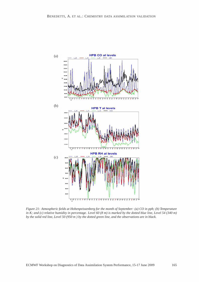
Hohenpeissenberg (HPB) is a singular mountain close to the Alps. The vertical modelled gradient in thePlanetary Boundary Layer for this site can be as large as 70% for CO and -64 % for ozone. There is alarge difference between station height and model orography. For example, with the 125 km orography(GEMS), the HPB peak cannot be resolved and the model only seeflat high terrain. With the 16 kmorography, the shape of the peak starts to being resolved andit is possible to identify a model level whichcould be representative of the air which is sampled at HPB. Inthis example, level 54 and level 50 aretested. Choosing a small-scale orography seems to better indicate to what extent the observed air wasinfluenced by surface processes or could be considered instead free tropospheric air.

Figure21shows CO, temperature and relative humidity at different model levels. A few key features arenoted for CO (shown in panel21a): there are large differences between levels 60 and 54; themodelledsurface diurnal cycle is very strong and level 54 and 50 are very similar. In constrast, panel21b showsthat for temperature there are small differences for level 54 and level 60. The values of temperature atlevel 50 appear very different from level 54. Moreover, it appear that for the 1st half of September level60 provides a better fit to the observations while for the 2nd half of September it is level 54 that providesa better fit. For relative humidity it is difficult to tell which level is most appropriate and it appears thatsub-scale influence is of paramount importance.

Conclusions from this study can be summarized as follows:

- Disregarding mountain observations is not good because there are few observations and thosesampling tropospheric air are extemely valuable.

- Considering model orography versus station height might be misleading for large-scale model(HPB would be below the T159 surface).

- Considering high-resolution orography helps to better judge the near surroundings of the station.

- Looking at temperature may confirm model level choice but one has to bear in mind that temper-ature and CO profiles have a very different shape.

7 Preliminary conclusions

Validation has been proven fundamental to assess the current status of the GEMS analysis system. Fu-ture improvements of the system, planned in MACC, will address some of the problems highlighted in



(a)

(b)

(c)

Figure 21: Atmospheric fields at Hohenpeissenberg for the month of September: (a) CO in ppb; (b) Temperaturein K; and (c) relative humidity in percentage. Level 60 (8 m) is marked by the dotted blue line, Level 54 (340 m)by the solid red line, Level 50 (950 m ) by the dotted green line, and the observations are in black.



the verification. The strategy for the verification has involved the use of available independent satellite,ground and aircraft-based observations of all GEMS tracers. Several metrics to measure the quality ofthe analyses have been used (bias, RMS, correlation, standard deviation, etc). The validation activityhas stressed the need for reliable, readily available, independent verifying data sets to provide a consis-tent record for the validations of successive versions of the the GEMS/MACC analysis systems. Theimportance of comparing analysis and observations in the most objective way was also highlighted (seemountain site example of section6.4.1). It is also important to underline that one should have realisticexpectations regarding the performance of the analysis which is limited by the forward model opera-tor, the forecast model, the prescribed background and observation errors and the inherent informationcontent of the observations.

References

Benedetti, A., J.-J. Morcrette, O. Boucher, A. Dethof, R. J.Engelen, M. Fisher, H. Flentje, N. Huneeus,L. Jones, J. W. Kaiser, S. Kinne, A. Mangold, M. Razinger, A. J. Simmons, and M. Sut-tie (2009), Aerosol analysis and forecast in the European Centre for Medium-Range WeatherForecasts Integrated Forecast System: 2. Data assimilation, J. Geophys. Res., 114, D13205,doi:10.1029/2008JD011115.

Engelen R. J., Serrar, S. and F. Chevallier, 2009: Four-dimensional data assimilation of atmosphericCO2 using AIRS observations,J. Geophys. Res., 114, D03303, doi:10.1029/2008JD010739.

Flemming,J., A. Inness, H. Flentje, V. Huijnen, P. Moinat, M. G. Schultz, and O. Stein, 2009: Couplingglobal chemistry transport models to ECMWFs integrated forecast system. Technical Memorandum590, ECMWF, 27 pp.

Hollingsworth, A., R. J. Engelen, C. Textor, A. Benedetti, O. Boucher, F. Chevallier, A. Dethof, H. El-bern, H. Eskes, J. Flemming, C. Granier, J. W. Kaiser, J.-J. Morcrette, P. Rayner, V.-H. Peuch,L. Rouil, M. G. Schultz, A. J. Simmons, and the GEMS consortium, 2008: The Global Earth–system Monitoring using Satellite and in–situ data (GEMS) Project: Towards a monitoring andforecasting system for atmospheric composition,Bull. Amer. Meteor. Soc., 89, 1147–1164, doi:10.1175/2008BAMS2355.1.

Inness, A., J. Flemming, M. Suttie, and L. Jones, 2009: GEMS data assimilation system for chemicallyactive reactive gases. Technical Memorandum 587, ECMWF, 26pp.

Morcrette, J.-J., O. Boucher, D. Salmond, L. Jones, P. Bechtold, A. Beljaars, A. Benedetti, A. Bonet,A. Hollingsworth, J. W. Kaiser, M. Razinger, S. Serrar, A. J.Simmons, M. Suttie, A. Tompkins,A. Untch, and the GEMS–AER team, 2008: Aerosol analysis and forecast in the European Centrefor Medium-Range Weather Forecast Integrated Forecast System: 1. Forward modelling,J. Geophys.Res., 114, D06206, doi:10.1029/2008JD011235.

Parrish, D. F. and J. C. Derber, 1992: The National Meteorological Center’s spectral statistical–interpolation analysis system.Mon. Weather Rev., 120, 1747–1763.

Acronyms

AEROCE = Atmosphere/Ocean Chemistry Experiment

AERONET = AErosol Robotic NETwork



AIRS = Atmospheric Infrared Sounder

CALIPSO = Cloud-Aerosol Lidar and Infrared Pathfinder Satellite Observation

CTM = Chemical Transport Model

GAW= Global Atmospheric Watch

GPS= Global Positioning System

GOME= Global Ozone Monitoring Experiment

IASI = Infrared Atmospheric Sounding Interferometer

IFS = Integrated Forecasting System

MIPAS = Michelson Interferometer for Passive Atmospheric Sounding

MLS = Microwave Limb Sounder

MOCAGE = Model of atmospheric chemistry at large scale

MODIS = Moderate Resolution Imaging Spectroradiometer

MOPITT = Measurements Of Pollution In The Troposphere

MOZAIC = Measurements of OZone, water vapour , carbon monoxide and nitrogen oxides byin-service AIrbus airCraft

MOZART = Model for OZone And Related chemical Tracers

OMI = Ozone Monitoring Instrument

SBUV = Solar Backscatter Ultraviolet

SCHIAMACHY = SCanning Imaging Absorption spectroMeter forAtmospheric ChartograpHY

TM5 = Test Model 5


Chemistry data assimilation validation using independent ...€¦ · Chemistry data assimilation...

Documents

Transcript of Chemistry data assimilation validation using independent ...€¦ · Chemistry data assimilation...