ChemicalChemical ThermodynamicsThermodynamics2013/20142013/2014

12th Lecture: Mixtures of Volatile LiquidsValentim M B Nunes, UD de Engenharia

2

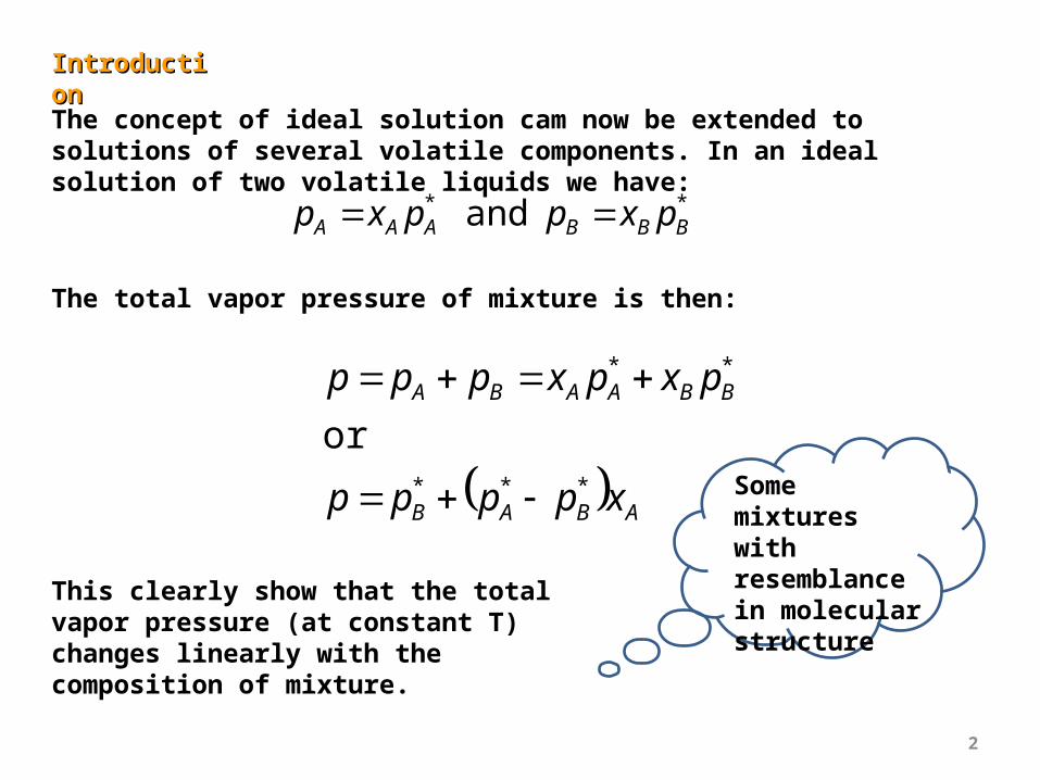
IntroductioIntroductionnThe concept of ideal solution cam now be extended to solutions of several volatile components. In an ideal solution of two volatile liquids we have:

** and BBBAAA pxppxp

The total vapor pressure of mixture is then:

ABAB

BBAABA

xpppp

pxpxppp

***

**

or

This clearly show that the total vapor pressure (at constant T) changes linearly with the composition of mixture.

Some mixtures with resemblance in molecular structure

3

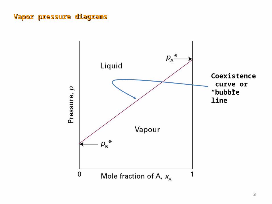
Vapor pressure diagramsVapor pressure diagrams

Coexistence curve or “bubble line”

4

The composition of vaporThe composition of vapor

The composition of liquid and vapor is not necessarily the same. It seems obvious that the vapor should be more richer in the more volatile component. Using Dalton`s law:

ppyp

py BB

AA and

It follows that: AB

ABAB

AAA yy

xppp

pxy

1 and

***

*

Inverting this expression we obtain: AABA

BAA yppp

pyx

***

*

Now, combining this two results:

AABA

BA

yppp

ppp

***

**

5

The composition of vaporThe composition of vapor

p

yA

pB*

pA*

Coexistence curve or “dew line”

6

Total phase diagram Total phase diagram

Combining both diagrams into one plot allow us to see the composition of both liquid and gas phase:

Above the liquid line the liquid phase is more stable. Bellow the vapor line the gas phase is more stable. In the middle region of the diagram we have the liquid vapor equilibrium, with two phases coexisting. At a given pressure we have a liquid with composition a in equilibrium with vapor of composition b.

7

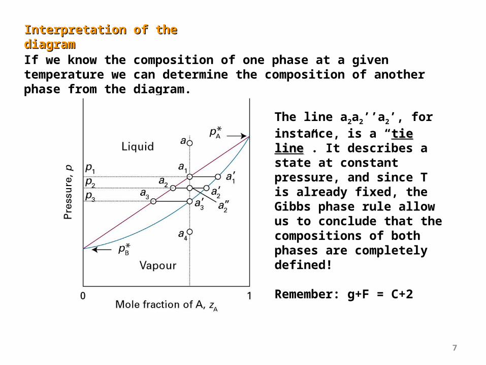
Interpretation of the diagram Interpretation of the diagram

If we know the composition of one phase at a given temperature we can determine the composition of another phase from the diagram.

The line a2a2’’a2’, for instance, is a “tie linetie line”. It describes a state at constant pressure, and since T is already fixed, the Gibbs phase rule allow us to conclude that the compositions of both phases are completely defined!

Remember: g+F = C+2

8

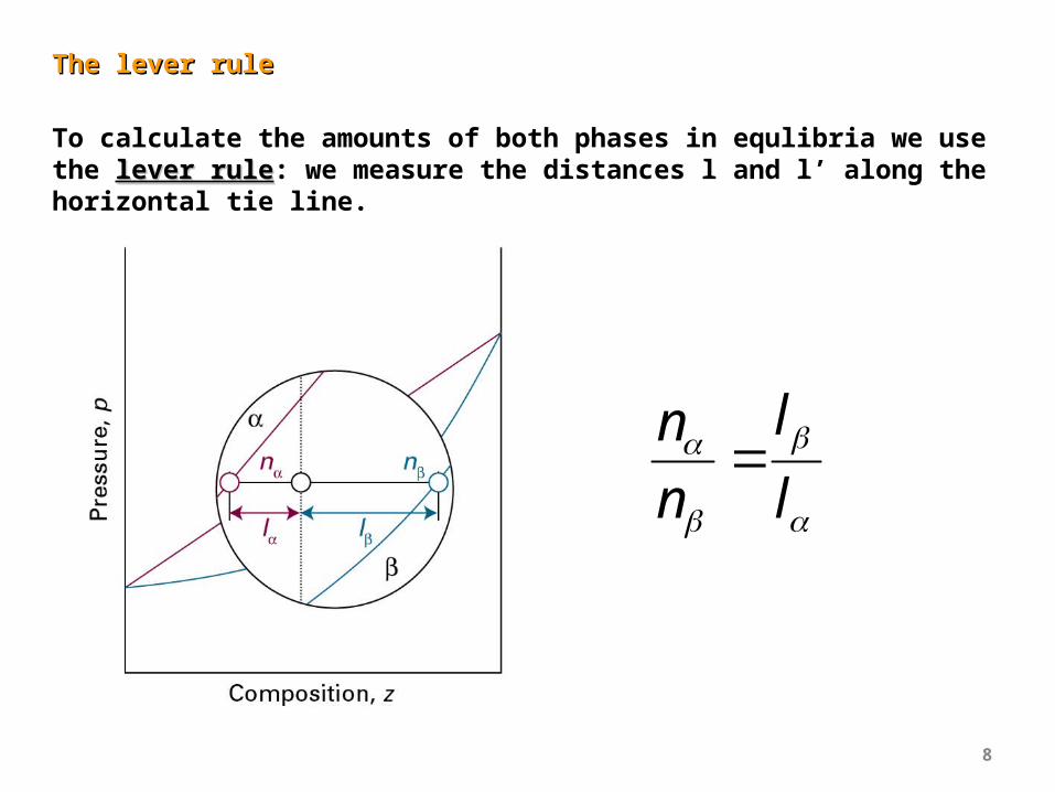
The lever ruleThe lever rule

To calculate the amounts of both phases in equlibria we use the lever rulelever rule: we measure the distances l and l’ along the horizontal tie line.

l

l

n

n

9

T-x DiagramsT-x Diagrams

Instead of T being fixed as in previous diagrams, we can keep constant pressure, and generate T-x diagrams. These diagrams have great importance in practical separation processes like distillationdistillation.

TB*

TA*

hea

t

vaporization

condensation

10

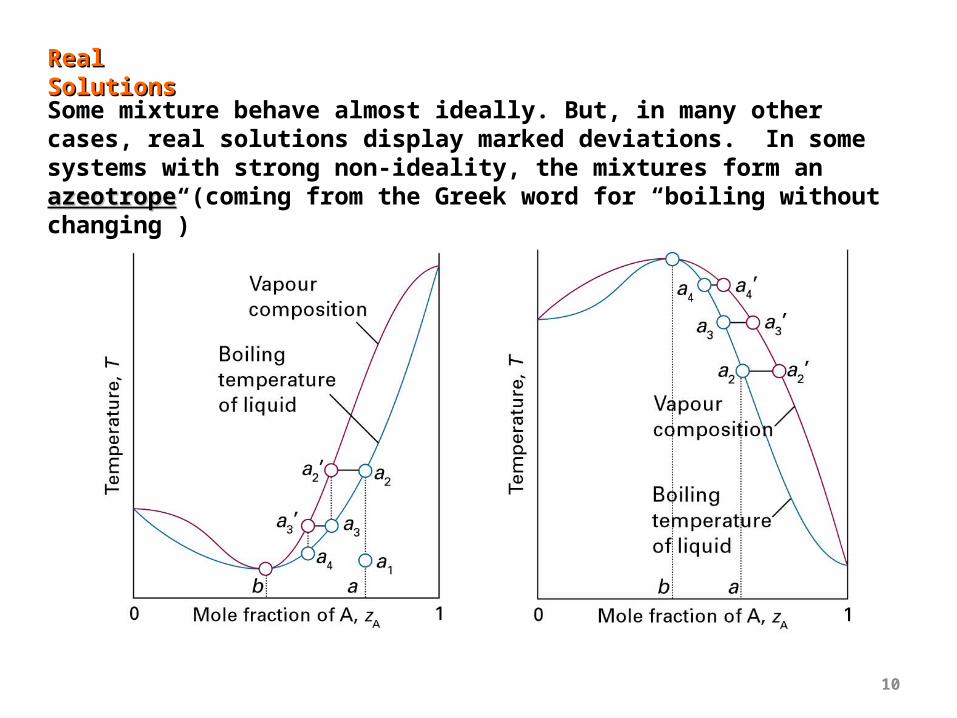
Real Real Solutions Solutions Some mixture behave almost ideally. But, in many other cases, real solutions display marked deviations. In some systems with strong non-ideality, the mixtures form an azeotropeazeotrope (coming from the Greek word for “boiling without changing”)

11

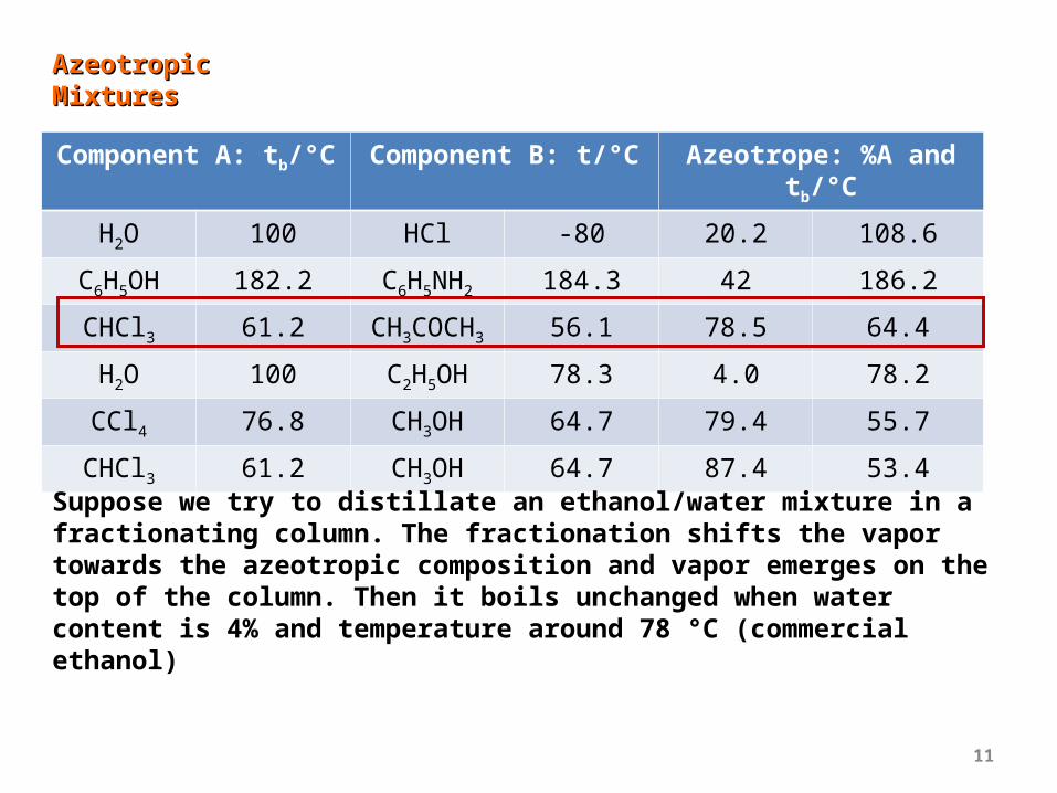
Azeotropic Azeotropic MixturesMixtures

Component A: tb/°C Component B: t/°C Azeotrope: %A and tb/°C

H2O 100 HCl -80 20.2 108.6

C6H5OH 182.2 C6H5NH2 184.3 42 186.2

CHCl3 61.2 CH3COCH3 56.1 78.5 64.4

H2O 100 C2H5OH 78.3 4.0 78.2

CCl4 76.8 CH3OH 64.7 79.4 55.7

CHCl3 61.2 CH3OH 64.7 87.4 53.4

Suppose we try to distillate an ethanol/water mixture in a fractionating column. The fractionation shifts the vapor towards the azeotropic composition and vapor emerges on the top of the column. Then it boils unchanged when water content is 4% and temperature around 78 °C (commercial ethanol)

12

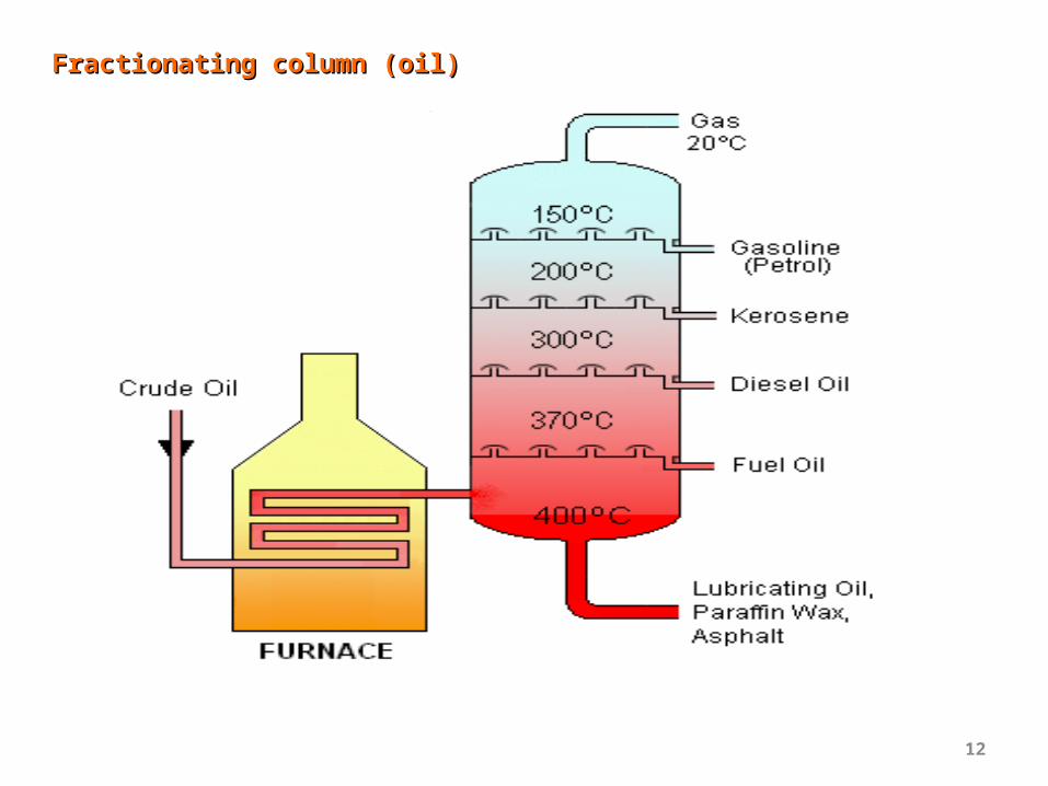
Fractionating column (oil)Fractionating column (oil)