Chemical reaction dynamics - Springer · Chemical Reaction Dynamics 233 The construction of the...
45
ChemicalReactionDynamics Part I: GeometricalStructure GEORGE F. OSTER & ALAN S. PERELSO~ Communicated by R. ARIS Abstract A mathematical theory of chemical reaction systems is proposed. Generic equations of motion are developed which separate equilibrium, nonequilibrium and stoichiometric aspects. The role of various constitutive assumptions is in- vestigated. Table of Contents 1. Introduction ................................. 230 2. Thermostatics ................................. 234 3. Dynamics .................................. 239 4. Constitutive Relations ............................. 255 References ................................... 272 1. Introduction 1.1. In classical mechanics the Hamiltonian model proposed that, out of all possible vector fields generating the equations of motion, one may consider only a restricted subclass: symplectic flows (ABRAHAM, 1967). All of the conclusions of classical mechanics derive solely from the properties of Hamilton's canonical differential equations under various constitutive assumptions, e.g. choice of Hamiltonian. In fact, even before a particular choice of Hamiltonian has been made, a great deal of information may be gleaned from the generic properties and form of the equations themselves, e.g. invariant volumes and restrictions on types of singularities. In a similar spirit, the modern theories of continuum mechanics seek to unify and place within a common conceptual framework all of the special models derived independently to describe particular continuum systems. In this paper, by adopting the viewpoint of dynamical systems and control theory, we shall endeavor to carry out an analogous program for chemical systems by con- structing a set of generic equations for chemical reactions. Recently, there have been a number of proposals to formalize the mathematical foundations of chemical reactions (WEI, 1962; ARIS, 1965, t 968; BOWEN, 1968 a; KRAMBECK, 1970; FEINBERG, 1972 a, b; HORN & JACKSON, 1972). Here, however, The work reported here was performed under the auspices of the U.S. Atomic Energy Commission.
Transcript of Chemical reaction dynamics - Springer · Chemical Reaction Dynamics 233 The construction of the...

Chemical Reaction Dynamics Part I: Geometrical Structure
GEORGE F. OSTER & ALAN S. PERELSO~
Communicated by R. ARIS
Abstract
A mathematical theory of chemical reaction systems is proposed. Generic equations of motion are developed which separate equilibrium, nonequilibrium and stoichiometric aspects. The role of various constitutive assumptions is in- vestigated.
Table of Contents
1. Introduction . . . . . . . . . . . . . . . . . . . . . . . . . . . . . . . . . 230 2. Thermostatics . . . . . . . . . . . . . . . . . . . . . . . . . . . . . . . . . 234 3. Dynamics . . . . . . . . . . . . . . . . . . . . . . . . . . . . . . . . . . 239 4. Constitutive Relations . . . . . . . . . . . . . . . . . . . . . . . . . . . . . 255 References . . . . . . . . . . . . . . . . . . . . . . . . . . . . . . . . . . . 272
1. Introduction
1.1. In classical mechanics the Hamiltonian model proposed that, out of all possible vector fields generating the equations of motion, one may consider only a restricted subclass: symplectic flows (ABRAHAM, 1967). All of the conclusions of classical mechanics derive solely from the properties of Hamilton's canonical differential equations under various constitutive assumptions, e.g. choice of Hamiltonian. In fact, even before a particular choice of Hamiltonian has been made, a great deal of information may be gleaned f rom the generic properties and form of the equations themselves, e.g. invariant volumes and restrictions on types of singularities. In a similar spirit, the modern theories of continuum mechanics seek to unify and place within a common conceptual framework all of the special models derived independently to describe particular continuum systems. In this paper, by adopting the viewpoint of dynamical systems and control theory, we shall endeavor to carry out an analogous program for chemical systems by con- structing a set of generic equations for chemical reactions.
Recently, there have been a number of proposals to formalize the mathematical foundations of chemical reactions (WEI, 1962; ARIS, 1965, t 968; BOWEN, 1968 a; KRAMBECK, 1970; FEINBERG, 1972 a, b; HORN & JACKSON, 1972). Here, however,
The work reported here was performed under the auspices of the U.S. Atomic Energy Commission.
Chemical Reaction Dynamics 231
we shall make no pretext of producing a complete axiomatic system; rather, we shall present in broad strokes an analytical structure whose details remain to be investigated.
In seeking to formulate a mathematical model for nonlinear chemical reaction dynamics, we were guided by certain considerations of consistency with other formalisms. For example, we require that the resulting structure be a rigorous extension of classical thermostatics. Furthermore, under appropriate constitutive assumptions, the equations should specialize to both the conventional linear irre- versible thermodynamic and chemical kinetic expressions. To this end, we shall derive a vector field which generates the generic equations of motion for chemical systems. These equations are expressed as a composition of maps which explicitly separates the roles of equilibrium properties, reaction properties and stoichio- metric constraints.
1.2. For chemical processes proceeding far from thermodynamic equilibrium, the mass action model has played a dominant role. This model, which has become almost synonymous with "chemical kinetics," has been successful in predicting rates of dilute gas reactions and has influenced almost all investigations of chemi- cal processes by means of statistical mechanics. However, its intuitive appeal in terms of a molecular collision picture, as well as the formal simplicity of writing kinetic equations, has influenced workers to retain the mass action model even for solution reactions by introducing various artifices such as fractional reaction orders, activity coefficients, and concentration dependent rate constants (DEN- mOH, 1971). The polynomial rate expression gradually evolved into an empirical correlation which, until recently, did not fit easily into a larger theoretical frame- work (FEINSERG, 1972a; HORN & JACKSON, 1972; HORN, 1972; KRAr~ECK, 1970; KERNER, 1972; SHEAR, 1968; SHAPIRO & SHA~LEY, 1965; WEI, 1965; ARIS, 1964). This is in contrast to the trend in modern dynamical theories (e.g. circuit theory and continuum machanics) where the distinction between the general dynamical laws and particular constitutive relations is clearly maintained. Chemical kinetics, moreover, has never been a natural extension of classical thermodynamics; thermodynamic "forces" play no role in conventional chemical kinetics. Early attempts by DE DO~ER and VAN RYSSELBERGHE (1936), ONSAOER (1931), PRI- GOOSE (1947), DE GROOT (1951), and others to formulate chemical reactions in terms of irreversible thermodynamics were successful only for steady states close to chemical equilibrium. The principal attraction of this formalism was the possibility of treating "coupled" processes phenomenologicaUy; the assumed validity of reciprocal constitutive relations played an important role in this approach (PRIGOGINE, 1967; TRU~I)ELL, 1969).
Several authors have investigated the possibility of treating chemical dynamics within a framework analogous to classical mechanics (KERNER, 1964; BraT, 1955; ONSAGER & MACHLUP, 1953). Much of the incentive for this effort lay in the esthetic appeal of mechanical variational principles which so elegantly summarize the equations of motion. Of course, such efforts were of limited validity since the constraint of symplectic flows, with their restriction to even dimensional systems, is simply too narrow a universe of discourse to encompass dissipative chemical processes.

232 G . F . OsTER&A. S. PERELSON
Recognizing the folly of forcing chemical reactions into the mold of classical mechanics, later authors began to formulate an independent mathematical struc- ture (WEI, 1962; WEI & PRATER, 1962; ARIS, 1965, 1968; BOWEN, 1968a, b; KRAMBECK, 1970). In discussing reaction stoichiometry, ARIS (1965) has noted that " . . . just as the algebra and calculus of tensors lies at the basis of continuum mechanics, so it will be found that the algebra of finite dimensional vector spaces lies at the basis of formal reaction kinetics... ". While this is certainly true for the stoichiometric aspects of kinetic systems, attempting to model the dynamics of nonlinear systems on a linear space creates some awkwardness, roughly comparable to solving a spherically symmetric problem in Cartesian coordinates. Moreover, inherent in a Euclidian vector space model are some unnatural identifications that should be avoided, e.g. the usual confusion of vectors and covectors via the canoni- cal Euclidian metric structure. Under the caveat that distinct mathematical structures be assigned to separate physical notions, such a metric structure should not be introduced into the problem capriciously, unless it is given naturally by the physics of the situation, as when, for example, the kinetic energy in classical mechanics is expressed as a quadratic form. Therefore, since we are concerned with nonlinear systems, we have chosen the language and formalism of differential manifold theory as the mathematical framework of our treatment.*
Aside from considerations of conceptual clarity involved in a geometric formulation, there is the practical aspect of dealing with systems whose state space is not Euclidean. This can come about in several ways. In chemical systems nonlinear constraint manifolds are most frequently encountered when various perturbation approximations are employed (e.g the "pseudo-steady-state" and "quasi-equilibrium" assumptions). Such nonlinear state manifolds may not possess a global coordinate system, making a manifold description mandatory. An example will be given in section 4.27.
1.3. While the mathematical language we shall employ is geometric in flavor, we have adopted the conceptual framework of modern dynamical systems and control theory.** (A formal definition of a dynamical system can be found in, say, WXLLEUS (1972) or ZADErI & DESOV_a (1963).) As a consequence, we shall take for granted that a mathematical model of a physical system has three aspects: (i) The notion of an internal "s ta te" , i.e. a set of measurements whose present values summarize past effects in a fashion sufficient to predict the future behavior of the system, assuming knowledge of future inputs. A differentiable manifold is as general a state space as we shall require. (ii) The notion of an input and an output space. (iii) The notion of a state transition function which generates out- puts from initial conditions and inputs via the intermediate state variables. Generally the state transition function is a group, or semi-group, generated by a set of differential equations.
* It is the authors' conviction that the approach through differential geometry can provide an intuitive mathematical framework for the investigation of nonlinear systems comparable to that provided by linear algebra for linear dynamical systems.
** Agis (1971) has previously suggested using ideas from the general theory of dynamical systems to treat the transient behavior of chemical reactors.

Chemical Reaction Dynamics 233
The construction of the generic equations of motion generating the state transition map for autonomous chemical systems is the central focus of this paper. Treatment of the input-output aspects will be deferred to Part II.
1.4. Our mathematical model for chemical reaction dynamics involves two aspects that should be emphasized. First, by treating the problem in a differential- geometric context it will prove natural to consider the state of a set of chemical reactions as a separate mathematical object, distinct from the state space charac- terizing the chemical species participating in the reactions. Each reaction, therefore, has its own constitutive relation in "reaction space", which is determined solely by steady state measurements. Moreover, each chemical species retains the same constitutive relation in "species space" that characterized it at thermodynamic equilibrium. In this way, the dynamical equations reduce in a natural way to classical equilibrium thermostatics, and the preeminent role of thermodynamic "forces" is maintained. Thus we achieve a true " thermodynamic" formulation of reaction dynamics.
Second, we view chemical systems as belonging to a special subclass of dynam- ical systems: so-called "interconnected systems" (WJLLEMS, 1972). In Part II we show that a chemical reaction system can be viewed as an interconnection of elementary systems in a precise sense. Most physical models, in fact, fall into this category. In the case of chemical systems this viewpoint permits us to introduce considerable simplification into the mathematical structure.
1.5. The organization of the paper can be understood in the light of the follow- ing definition: A chemical system, CS, consists of five objects {Jff, ~/f, #, A, -~) where
(1) .,4" is a differentiable manifold equipped with
(2) a differential form ~: ~ ~ T* ~r ;
(3) a second manifold, J/C, equipped with (4) a "bundle map" A: T*.4/-~ Td/ ; and
(5) a map ~ o : ~ ' ~ f ' .
The relations between these objects is summarized in Fig. 7; the remaining body of Part I is devoted to an exposition of this structure and its interpretation in conventional chemical terms.
In section 2 we first fix some geometric notations and then discuss the thermo- statics of a chemical system in terms of the manifold .,4" and the differential form /~. In section 3 we introduce the reaction manifold, .4/, and equip it with the re- action constitutive relation, A. The two manifolds are related by the map, La~o, which embodies the law of definite proportions. Next the dynamics of near- equilibrium chemical processes is discussed, both as a pedagogical introduction to the complete structure and to make contact with the familiar linear irreversible thermodynamic formalism. Nonlinear reactions proceeding far from thermostatic equilibrium necessitate several technical modifications and are treated next. Finally, in section 4, the consequences of several common constitutive assumptions are catalogued. In Part II. we show that the entire mathematical model can be concretely realized in terms of a generalized network representation. That is,
234 G.F. OSTER ~z, A. S. PERELSOI'4
an isomorphism between the mathematical structure of chemical reaction net- works and abstract network theory is established. We feel that the "n-por t model" developed there is an attractive and natural setting in which to discuss the phenomenological aspects of nonlinear reaction networks and offers substantial advantages over other representations of chemical reactions. A graphical notation has been devised, which provides an intuitive shorthand for the underlying mathe- matical structure, so that the equations of motion for complex systems may be obtained directly from the diagram. Using this notation as a guide allows us to introduce the input-output aspects of our model in a natural fashion. Finally, we extend the structure to include mass transport as well as chemical reaction.
Throughout, our intent is to elucidate the structure of the equations of motion generated by our assumptions. The dynamical consequences of the structure is pursued only within the context of certain commonly encountered constitutive assumptions. Indeed, one of the contributions of this work is to delineate more clearly the distinctions between topological, geometrical and constitutive relations for chemical systems.
2. Thermostat ics
2.1 Notation. We shall assume that the reader is acquainted with the basic notions of differentiable manifold theory; standard references include LANG, 1972; WARNER, 1971; Looms & STERNBERG, 1968; and BRICKELL d~ CLARK, 1970.* The following notations will be adhered to throughout:
NN+ the positive orthant of N-dimensional Euclidean space
IRN+ the non-negative orthant of N-dimensional Euclidean space
(Jff, tpa ) differentiable manifold JV with local charts, q~o, aeA, some index set, and dimension N.
TJff tangent bundle of d .
Tx~ r tangent space to ~ at x
T* .W" cotangent bundle of J/"
T* J/" cotangent space to .A r at x
n. natural projection n.: T~4r~JV, n. (v)=x for v~Tx.h r
n" natural projection n" : T*./V'.-,,A r, n ' (w)=x for w~T*.A".
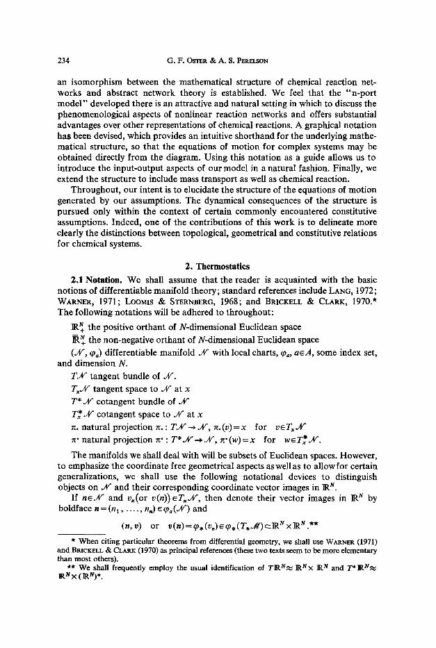
The manifolds we shall deal with will be subsets of Euclidean spaces. However, to emphasize the coordinate free geometrical aspects as well as to allow for certain generalizations, we shall use the following notational devices to distinguish objects on ~ r and their corresponding coordinate vector images in ]pN.
If neJV" and vn(or v(n))eT,.A/', then denote their vector images in IR N by boldface n= (n l , . . . . . n,) ~pa(M/') and
(n,v) or e(n)=q~,(Vn)~tp,(T,~)cIRN X~,N. **
* When citing particular theorems from differential geometry, we shall use WARNER (1971) and BRICK~LL & CLARK (1970) as principal references (these two texts seem to be more elementary than most others).
** We shall frequently employ the usual identification of Tp-N~ p, Nx ~,N and T* F,N~, F.HX (IRN)*.

Chemical Reaction Dynamics 235
Some conceptual clarity is also obtained if we distinguish between the coordi- nate functions n ~ on X and the components of vectors in p N, denoted n~. That is, if n e..4/', n e IR N and uS: IRN--* IR are the usual coordinate functions on ]R N, then
u~(n)=n~. We define n I by the compomion n~=u% q~a: JI/'--, ]R (we shall use o to denote the composition of functions: n~(n)=u% q~,(n)=u~(q~,(n))=u~(n)=n~.).
For each point neAP, a basis for the vector space T,~" is given by the coordi-
O v'(n) - ~ . where vi(.): JV" --, IR. nate derivations ~ ; so if v.eT..A/', v .=
The coordinate functions on T.hr will be denoted (n% n, i/i) where n% n(v.)=n~ and//~(v.)= v~(n). The dual basis on T'de" is given by the coordinate differentials dn~., so if
< ,+L> r.o~T*.A/', co,,= Z w,(n)dn' and dnk., =6f, i = 1 n
where 6~ is the Kronecker delta and w~(-): Jr'--, P,.
A curve F on a manifold Jr" is a map F: ]17,--..4/'. The lifted curve is defined as the map/~: ~ - - , T~r by P(t)=(F(t), P(t)), where -#(t) is the tangent vector to F at t. In coordinates it is customary to write t~(n~oF, ..., nNolO (t)=n(t) and t . ( i / 1 o _F . . . . , i/no F) (t) =//(t).
If F: .~/--, ~ , m~n=F(m) is a differentiable map between manifolds dr' and diP, then the corresponding vector map is denoted by boldface F: ]R M ~ p N. F=cp.oFo~k~ -a (where ~b b and tp. are charts mapping d / o n t o ]R u and de" onto ]pN, respectively) is also called the local representative of F. The tangent map F,(m): Tm~ll~Trt=)r r, vm~wetm) has as a local representative the Jacobian DF (m): Tm ]R M-, Tr(=) ~N, (m, v) ~, (F (m), DF(m) r). Similarly, the cotangent map F*(n): T*aff-~T*r has as a local representative the (vector) adjoint map DF(m)r: T* P.'~--* T* ]R u. This notation is summarized in Fig. 1.
F.(ml
F
DF(m)T'w Tm]R M DFIm) T / /c~ ToR" [ / ~,~ v(m} DF(m] ~,
m [ i v i [n'~:n
~ I I m i n i
Fig. 1
236 G . F . OSTER ~, A. S. PERELSON
n ~ UQ c.h"
.
~0Q ,a i'1 i
h e R . N = P~.3 n i
Fig. 2
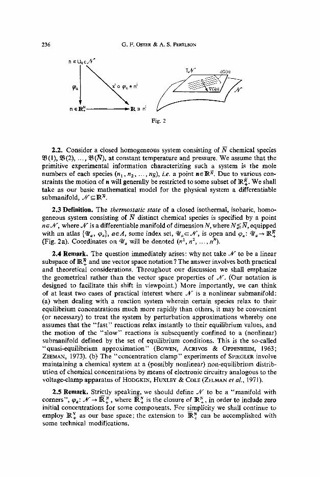
2.2. Consider a closed homogeneous system consisting of _N chemical species ~B(1), !B(2), ..., ~B(.N), at constant temperature and pressure. We assume that the primitive experimental information characterizing such a system is the mole numbers of each species (nl , n2, . . . , nn), i.e. a point ne]R~. Due to various con- straints the motion of n will generally be restricted to some subset of ]I(~+. We shall take as our basic mathematical model for the physical system a differentiable submanifold, j t f _ IR~.
2.3 Definition. The thermostatic state of a closed isothermal, isobaric, homo- geneous system consisting of N distinct chemical species is specified by a point n ~.s where ~V is a differentiable manifold of dimension N, where N < N , equipped with an atlas {q/o, q~,}, a~A , some index set, q / ~ Jff, is open and (Pa: ~ IR~+ (Fig. 2a). Coordinates on q/, will be denoted (n 1, n 2, ..., nN).
2.4 Remark. The question immediately arises: why not take ~ to be a linear subspace of ]P~+ and use vector space notation ? The answer involves both practical and theoretical considerations. Throughout our discussion we shall emphasize the geometrical rather than the vector space properties of JV. (Our notation is designed to facilitate this shift in viewpoint.) More importantly, we can think of at least two cases of practical interest where ./r is a nonlinear submanifold: (a) when dealing with a reaction system wherein certain species relax to their equilibrium concentrations much more rapidly than others, it may be convenient (or necessary) to treat the system by perturbation approximations whereby one assumes that the " f a s t " reactions relax instantly to their equilibrium values, and the motion of the " s low" reactions is subsequently confined to a (nonlinear) submanifold defined by the set of equilibrium conditions. This is the so-called "quasi-equilibrium approximation" (Bow~N, Acglvos & OPPENHEtM, 1963; ZEEMAN, 1973). (b) The "concentration clamp" experiments of SPIE6LER involve maintaining a chemical system at a (possibly nonlinear) non-equilibrium distrib- ution of chemical concentrations by means of electronic circuitry analogous to the voltage-clamp apparatus of HODGKIN, HUXLEY & COLE (ZELMAN e t al., 1971).
2.5 Remark. Strictly_ speaking, we should define Jff to be a "manifold with corners", q~,: .IV ~ ~(+N, where IR~ is the closure of ]RN,, in order to include zero initial concentrations for some components. For simplicity we shall continue to employ ]R~ as our base space; the extension to p.N+ can be accomplished with some technical modifications.

Chemical Reaction Dynamics 237
2.6. In general, a constitutive relation associates covariant with contravariant quantities. In particular, we wish to assign to each chemical species, ~3(i), its chemical potential,/~. (The subscript i will always refer to chemical species.) The following definition conforms to common usage.
2.7 Definition. A capacitive, or thermostatic constitutive relation on JV is defined as a continuous cross-section of the cotangent bundle T ' J / ' . In particular we have:
2.8 Definition. The chemical potentials /z~(') assigned to each species ~( i ) form the components of a differential form, i.e. a covector field on ~ : *
p: ,4: ~ T*~4 P,
n ~/~n"
In what follows we shall generally assume that/~ is at least of class C ~.
2.9 Remark. Under the coordinate charts, {tp*}, for T 'a f t , we may identify T*Jff locally with IR N x (IRN) *. Hence the covector #(n) is represented locally by the 2N-tuple (n~, n2, ..., nN; #1, /~Z, .. . , I~N)=( n, !~).
2.10 Remark. A commonly employed capacitive constitutive relation is the ideal dilute solution defined by
#9 + R T In ~ (2.10-1) ni v
where V is the volume and ~t~ is a function of temperature and pressure. Although it will play no immediate role in the ensuing development, the
following property is usually postulated for p(-).
2.11 Postulate. The 1-form/~ is closed, i.e. d/~ = 0, and .h: is simply connected.** This guarantees that/~ is exact, i.e.
i~=dG (2.11-1)
for some real-valued function G: JV ~ JR. Therefore G (the Gibbs free energy) fibers JV by its level sets Fig. 2 b. G is useful as a Liapunov function for thermo- dynamic systems (WEI, 1962).
2.12 Remark. Expanding dG in coordinates dn ~ on T*JV, we regain the familiar Gibbs Equation
N
dG~= ~. Iz~(n)dn ~ (2.12-1) i=1
i.e. aG (n), ~G aG )
nl, ne, . . . ,nN; (n) . . . . . (n)
- - ( , ,
* /z is related to the "Gibbs form" of HERMANN (1973). ** d is the exterior derivative, do d ( . )=O (e.g. WARNER, 1971, p. 65; LOOMIS & STERNaERG,
1968, p. 438).

238 G . F . OSTER & A. S. PERELSON
Then
o r
N
d o d G = O = ~ dl t i^ dn ~ i = l
= ~ , ( Olti. O~tJ~dniAdn j t j < i \ O n J On'/
(2.12-2)
d G ~ V G = ~--~n-rn
The trajectories of VG are curves such that
d ds r va(r
It is important to notice that the parameter s cannot be identified with "real t ime". That is, the vector field VG does not generate the flow of an actual dynamic process;
ds_ 0 its integral curves cannot be reparametrized by time, t, except in the limit d t
(i.e. for "infinitely slow processes"). In order to parametrize trajectories on by "clock t ime", we must account for an additional physical phenomenon: the velocity dependent "dissipation" accompanying all finite rate processes.
DI~=DI ~r, (2.12-3)
which are the usual Maxwell relations. N
Call pc & ~ dl~iAdn i the "reciprocity fo rm" (BRAYTON, 1971); in section 4 i = l
we shall give a geometric interpretation of this 2-form, The vanishing of Pc may be taken as a constitutive assumption for equilibrium systems. An analogous 2-form, PR, will appear when we discuss irreversible processes.
The same sort of construction arises in mechanics in the following way. The cotangent bundle to a differentiable manifold carries a "canonical" (i.e. intrinsi- cally defined) antisymmetric, bilinear form I2: T*./V ~ T* (T*.4/') (cf. LOOMIS & S~RNBERG, 1968, p. 515). By use of Darboux's theorem, f2 can be written locally as f2 = ~ dpi A dq i, where P i and qi are coordinates on T*sff (momenta and position, respectively). This 2-form is used to generate Hamilton's equations of motion on T*./r (cf. section 3.38). The chemical equations do not arise in this way, but we note that the reciprocity 2-form Pc defined on Jff is just the pull-back to Jff of the symplectic form on T*.A/', pc=p * f2.
2.13 Definition. In order to connect points on sff corresponding to different chemical compositions, we define a chemical process to be a continuous curve r I R ~ W , s ~ r
2.14 Remark. Although a metric is not given a priori on W, it is common to employ the Euclidean metric on IR n, gr ( - , - ) : R n x IR~ ~ ]R to convert covectors to vectors by the usual isomorphism: gr: (]R~)*~ ]R~. This metric may be em- ployed on .#" to define a gradient vector field
Chemical Reaction Dynamics 239
2.15 Remark. The singularities of the vector field VG correspond to the loci of thermostatic equilibria. These loci may also be characterized by a constrained extremum of G in the usual fashion (SHAPIRO & SHAPELY, 1965; CALLEN, 1960; OSTER • PERELSON, 1973).
3. Dynamics
In this section we derive a canonical form for the differential equations de- scribing chemical reaction dynamics in closed isothermal, isobaric systems. Rather than develop the dynamical equations for the general case right off, we shall pro- ceed by a more redundant, but pedagogical route and first treat the simpler case of near-equilibrium reactions. This will allow us to make contact with the familiar linear irreversible thermodynamic treatment of chemical reactions, and to motivate the ensuing technical modifications necessary to treat nonlinear systems. First, however, we estabIish some chemical notations.
3.1 Definition. A chemical reaction involving N species ~B(1), ~B(2) . . . . ~3(N) may be expressed in the general form:
~., v ~ ( i ) ~ - ~ vP~B(i). (3.1-1) 1=1 i = l
The coefficients v~ and v~' are non-negative integers, the reactant and product stoichiometric coefficients, respectively. Note that the sum extends over all 3V species to allow for the possibility that a given species can participate in a reaction as both product and reactant (e.g. an autocatalytic reaction).
The formal linear combinations of species occurring in equation (3.1-1) are called complexes, ~ (HORN & JACKSON, 1972). A chemical reaction may therefore be written in the form
cgR ~.~ c~P (3.1-2)
where fiR& ~ v~ ~B(i) is the reactant complex and cgP~ ~ vf ~B(i) is the product iffiffil t=1
complex. We say species ~( i ) is a member of the reactant (product) complex if �9 ~(v P) is non-zero.
A set of .~ homogeneous reactions, involving N distinct chemical species, occurring at constant temperature and pressure, will be called a reaction set, and denoted t 2 ~ . The reactant and product complexes for the k th reaction will be denoted cgR(k) and cge(k) respectively. The subscript k will be used to denote chemical reactions.
The ~ x .M matrix, v ~, with a elements vik (the reactant stoichiometric coefficient of species i in reaction k) will be called the reactant stoichiometric matrix. Similarly, the matrix with elements v~ek, denoted by v e, will be called the product stoichio- metric matrix. The (conventional) stoichiometric matrix is given by
A v = - v g + v P. (3.1-3)
We also define the N x 2 J~ complex stoichiometric matrix as
0~ v R - [ , r e ] . ( 3 . 1 - 4 )
The negative sign is introduced for reasons of consistency with certain thermo- dynamic formulas.
240 G.F. OSTER & A. S. PERELSON
The number of stoichiometrically independent reactions in I 2 ~ is the rank of v. If rank (v) = M, then t2~ ~ wdl be called an independent reaction set; otherwise, I 2 ~ is said to be stoichiometrically dependent. The ranks of v R and v p are the number of linearly independent reactant and product complexes, respectively. The rank of 9 is the number of independent complexes. If we denote by C R, C P, and C the sets of reactant complexes, product complexes, and complexes, respec- tively, i.e.
c R = ( C R ( k ) , k = 1 . . . . .
C = { C ( k ) , k = 1 . . . . .
C=CR u C r, then
a) if C R = C e, rank (~) = rank (v R) = rank (v e);
b) if CRc~CP=r rank (~)=rank (vR)+rank (re).
3.2. Remark. A formal description of chemical kinetic systems in terms of complexes was developed by HORN & JACKSON (1972). Algebraic aspects of reaction stoichiometry have been investigated by ARIS (1965).
3.3. In order to discuss the dissipative aspects of chemical reactions separately f rom considerations of chemical equilibrium, we consider the reaction process itself as a separate mathematical object.
The fact that each reaction, which generally involves several chemical species, may be characterized by a single coordinate, is a consequence of the " l aw of definite propor t ions" . Here we simply take this experimental fact as our license to characterize a reaction set f2~t by a point ~E(~ 1 , . . . , ~r)~]R ~t.
3,4 Remark. Just as the thermostatic state may be confined to a nonlinear submanifold of species space, ]Rg, so may the locus of reaction states, ~, be con- fined to a submanifold of the reaction space, R u . This can come about as a result of perturbation approximations also (cf. 2.4). In modelling complex reaction sets, it is frequently the case that certain species are present in much smaller amounts than others. The "pseudo-steady-state-hypothesis" assumes that the changes in the concentration of these trace elements occur on a time scale much shorter than the other species. Thus the motion of the system in R ~t is confined to a submanifold, M___R ~r. The system equations then consist of a set of M < M differential equations and ( M - M ) algebraic equations (HEINEKEN, TSUCHIYA & ARIS, 1967). Consequently, the state manifold for a reaction set is generally a nonlinear submanifold of R ~ (cf. 4.27).*
3.5 Definition. The state o f a reaction set 12~t is defined by a point r on a differentiable manifold M, modelled locally on R u, M < M , with charts Cb:
--' ]R M, b belonging to some index set B and ~ ~ M is open.** Coordinates on will be denoted (41, r "" , ~M).
* The notion of "reaction coupling" also implies a constraint amongst the reaction advance- ments, e.g. f(~) ----- 0. The physical interpretation of such constraints is not clear except in the case of stoichiometrically dependent reactions (PINGS & NESEr~ER, 1965).
** We have employed the same letter, M, to denote both the manifold and its dimension, i.e. R M Context will ensure there is no danger of confusion.
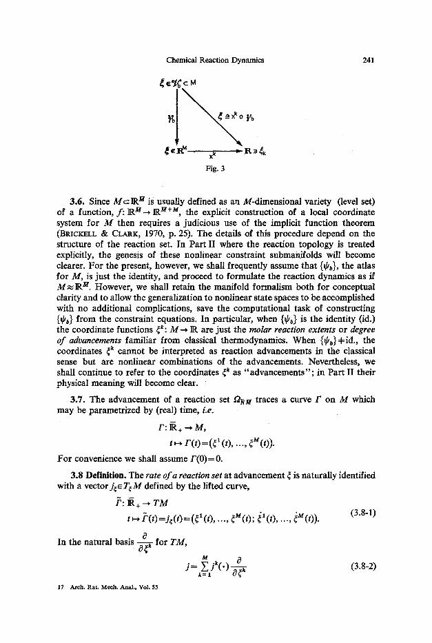
Chemical Reaction Dynamics 241
, ~ e R ~ x ~ *" R~,~k
Fig. 3
3.6. Since M ~ R n is usually defined as an M-dimensional variety (level set) of a function, f : R ~t--} lg ~t+t~, the explicit construction of a local coordinate system for M then requires a judicious use of the implicit function theorem (BRICKELL & CL~tK, 1970, p. 25). The details of this procedure depend on the structure of the reaction set. In Part II where the reaction topology is treated explicitly, the genesis of these nonlinear constraint submanifolds will become clearer. For the present, however, we shall frequently assume that {~bb}, the atlas for M, is just the identity, and proceed to formulate the reaction dynamics as if M ~ R ~. However, we shall retain the manifold formalism both for conceptual clarity and to allow the generalization to nonlinear state spaces to be accomplished with no additional complications, save the computational task of constructing {~kb} from the constraint equations. In particular, when {g/b} is the identity (id.) the coordinate functions r M--} ]R are just the molar reaction extents or degree o f advancements familiar from classical thermodynamics. When {ff~}=l:id., the coordinates ~ cannot be interpreted as reaction advancements in the classical sense but are nonlinear combinations of the advancements. Nevertheless, we shall continue to refer to the coordinates ~ as "advancements"; in Part II their physical meaning will become clear.
3.7. The advancement of a reaction set f 2 ~ traces a curve F on M which may be parametrized by (real) time, i.e.
F: R+ "--} M,
r ( t ) = ( r l(t), ...,
For convenience we shall assume F(0)= 0.
3.8 Definition. The rate o f a reaction set at advancement ~ is naturally identified with a vectorjr defined by the lifted curve,
F: ~+ --} T M
t ~ I ' ( t )=jr ..., ~u(t); ~l(t) ..... ~ ( t ) ) . (3.8-1)
0 In the natural basis ~ r for TM,
a j = ~ j ~ ( . ) - - (3.8-2) ~=1 O~ ~
17 Arch. Rat. Mech. Anal., Vol. 55
242 G.F. OSTER ,~ A. S. PERELSON
where the function j k ( ' ) : M-+ ~( is the reaction rate of the k th reaction. Via the coordinate charts ~/b, ~bb,~ F defines a vector field on ~ u :
t - - (r ~(t)).
In the ensuing development we shall state key formulas in both their coordinate free form and locally in vector notation.
3.9. As mentioned previously, a constitutive relation relates a contravariant to a covariant quantity. For each advancement 3, the constitutive relation for a reaction set relates the reaction velocity jr162 to a covector in T~. M (i.e. the reaction constitutive relations defines a "bundle m a p " , T* M ~ TM). Although there are, as yet, no naturally defined elements of T* M, as there were for T ' a t ' , the reaction stoichiometry provides us with a method of transferring differential forms on X to M.
3.10. The stoichiometry, together with an initial set of mole numbers, n~ ", defines a C ~~ map between 1~. n and ~,~ as follows.
Let H : R ~ x IR ~ x IR ~r--+ IR ~ be a C ~ map defined by
(n, ~, G) ~ n + v (G-r (3.10-1) A choice of initial mole numbers n o and an imtial advancement r = ~o determines
a C ~~ map, L.o, io~H(n ~ ~o,.): ~.~r__,~,~, defined by
L.o. go: IR~ ---, IR ~ ~ n o +v(G-G~ (3.10-2)
With no loss in generality, we assume G ~ 0, and denote L.o go simply as L=o.
When the species and reaction spaces are nonlinear submanifolds, L.o induces a map, L.o: M--, ,/f'. If i: Mc--,]R~ is the natural injection of M into IR ~ obtained by regarding points on M as points in IR ~, then L.oo i: M-- , ]R~. Let r ]R~ ~r r be a parametrization for ~r the method for selection of coordinates will be readdressed in Part I I since it involves considerations of reaction topology. Then
define L .o~r i: M ~ . Unless stated otherwise, we shall restrict the re- mainder of our considerations in Part I to the case f, i = identity, ,M = M, N = N and the manifolds M= IR M and n = IR ~r However, we shall continue to adhere to the geometric language so that the generalization to non-Euclidean manifolds is automatic.
Associated with L.o are its derivative maps Lno and L.o. To shorten the notation, we shall denote these maps L , and L*:
L,: TM --+ Tell',
L*: T'A:--+ T ' M , In coordinates
L.(G)=DLno(G)=v
je ~/tLno(g), (3.10-3)
Ix~ ~ L* p~. (3.10-4)
V~je~ ~. (3.10-5)
Since the number of linearly independent reactions is always < N - 1 (ARIS, 1965), L , (G )= v has rank < N - 1 , V GeM. Therefore we have
3.11 Proposition. Lno is not onto.

Chemical Reaction Dynamics 243
3.12 Proposition. If f2~u is an independent reaction set (i.e. rank v= M), then (a) L* is surjective, (b) L . is injective.
Proof. (a) by assumption, rank L* = M. (b) rank L , + nullity L , = M. Therefore nullity L* = 0.
3.13 Definition. The thermodynamic affinity of a reaction set at advancement is an element of T~ M defined by
a ~ -- L* #t.,o. (3.13-1)
The minus sign is due to thermodynamic convention. In local coordinates this reduces to the usual definition ~ = - v r / t .
Expanding ctr in the natural basis set {d~ k} for T~ M gives
M
ar = ~ ak(O d~ ~. (3.13-2) k = l
The function ~k: M ~ IR is the affinity of the k th reaction.
Notice that since tt is exact (/t = dG for some G: ~ff -~ 1R) L,o induces a real valued function on M, t~: M-~R, ~ ( - L * G ) ( 0 so that the affinity covector field on M is also exact:
~t= - L* I~ = - L* d G = d ( - L* G) ~ dG. (3.13-3) In coordinates,
k ~ G ( O k M M
a k ( O d r =,=-- O g ' ~ l ~ d r (3.13-4) k =
3.14. At this junction we distinguish two classes of reaction dynamics: (a) reac- tions whose rate can be completely specified by the chemical affinity, (b) reactions whose rates are not expressible as a unique function of ~ alone. The distinction between these two cases is essentially the distinction between a thermodynamic and non-thermodynamic description of reaction rates. For simplicity, we treat the thermodynamic case first.
3.15 Definition. A reaction set f2s~ will be said to have a thermodynamic reaction constitutive relation if there exists a C t fiber map, 2~: T ~ M ~ T r ~r162 V GeM. The bundle map 2 will be called a dissipative, or resistive constitu- tive relation (see Fig. 4).
Z4 .T M
~EM
F i g . 4
17*

244 G.F. OSTER t~ A. S. PERELSON
Note that 2 replaces the Euclidean metric g r ( ' , ' ) on M, as a method for converting differential forms into vector fields.* Viewed another way, the resistive constitutive relation is analogous to a nonholonomic constraint on the reaction advancements, ~ (t); i.e. 2 acts only on the second factor:
~'(~)--- ~.(4(~)). Or, in coordinates
(r ~) • (r x(~)).
3.16 Definition. We call a point p = (~o, 4 (~o)) e T* M x T M an operating point. Then the incremental resistive constitutive relation at an operating point p is the tangent map of 4:
4. ,0: T~o(T*M) ---, Ta~,o)(TM), (3.16-1)
~ o " 4 , ~o (6 ~o) = ~J~o)"
In coordinates 4.~o= D4(r ~to): ]R u--, ]R u, where the Jacobian acts only on the third factor: (~o, Gto; (5 ~) ~ (r ~to; 6j). In the treatment of the linearized equations of motion, we shall frequently omit the operating point and write simply
6j -- 4 . (6 ~). (3.16-2)
3.17 Remark. Note that 2 ( ' ) is not assumed to be linear. However, definition 3.15 includes the constitutive relation employed in conventional irreversible thermodynamics. That is, if 2 is linearized about an equilibrium point, (7, 8), then 4.(7, ~)~D~(~) is the phenomenological matrix of Onsager coefficients. It is an additionial constitutive assumption that D;t(~) be symmetric or diagonal. The consequences of various physically motivated constitutive relations will be in- vestigated in section 4.
3.18. We are now in a position to assemble the equations of motion for the thermodynamic case. Because of the constraints imposed by the reaction stoichio- merry ( i .e .L . is not surjective), the dynamics are most naturally formulated on M rather than ~r. Once the equations are solved for the flow, the trajectories on M may then be mapped back to Jff via L, , . Alternatively, the vector field defined on M may be mapped via L . into a vector field defined on a submanifold of Jf" (cf. 3.20).
3.19 Definition. Let Y.,: M---} T M be the vector field on M corresponding to an initial set of mole numbers, n o , given by
Y,o ~ 4 o ( - L*) o/to L,o. (3.19-1)
This vector field can be " read off" the mapping diagram illustrated in Fig. 5. A curve F: IR+ --} M will be called a reaction trajectory if it is a solution to the equa- tions of motion generated by }'no:
d dt r(t)=Y.o(r(t)), r (o)=o. (3.19-2)
* 2(. ) is related to the Legendre transform, viewed as a fiber map T'M--} TM (MAcLANE, 1968).

Chemical Reaction Dynamics 245
T./J/' ~ L~ TM
T ~ = T ~" M -L*
Fig. 5
The reaction trajectories may be mapped via L,o to yield the dynamical trajectories on ~" :
7(t)=L~oo F(t), 7(0)= n o (3.19-3) where y: R+ ~ .
In local coordinates, points on y(t) are given by
n(t)=n~ n(O)=n ~ (3.19-4) where
~( t )=g( - -vrp(n~162 d~(0) =0. (3.19-5)
Note that since we have set ~(0)= 0 (cf section 3.7), Y~. does not generate a flow by varying the initial conditions. However, by viewing n o as a parameter, we can define a flow ~ on M with parameter space r165
~: JR+ x X x.Ct'-,~',
(t, n ~ ~(0) =0) ~ ~(t) (3.19-6)
such that for each n~ ~/', the curve t ~ ~ (t, n ~ 0) is a reaction trajectory satisfying the initial condition ~(0, n ~ 0).
3.20. In the above treatment M has been chosen as the state space rather than r since, for stoichiometrically independent reactions, there are at most N - 1 advancements. However, we see no compelling reason for requiring our reaction sets to be independent. Our view is that we are given an actual set of chemical reactions which are kinetically independent, but possibly stoichiometrically dependent, whose dynamics we wish to model. If g2Nu has only r < M independent reactions, then in order to maintain a minimal representation of the system dyna- mics the equations of motion should not be formulated on M. The range of L,o defines an r-dimensional manifold ~ which can be parametrized by n 1 . . . . . n" (providing L*(dn 1 ̂ ... ^ dn')=~O, i.e. rankL , o=r). The coordinates on ~ , tf:
~ ]R are related to the actual (" kinetically independent") reaction advancements, ~ : M ~ R (by ~t=L*rf). The vector field Y,o on M can be transferred to ~ by defining the map L,o: M ~ ~ such that L,o = ia~o L,o, where i~: ~ r is the natural injection. Then, on ~ , the equations of motion can be written
,~ = x ( , 7 )

246 G . F . OSTER & A. S. PERELSON
T~ 4 "L~ TM
T'*.h/" " -" -d*
Fig. 6
where X: ~ --. T ~ is given by (see Fig. 6)
X = L , . o 2o - L*/~ o i~.
These are a set of only r < M independent differential equations, defined on (but not, in general, on all of Jff)*.
If ON u is a stoichiometrically independent reaction set, it is not necessary to transfer the equations to ~ . However, even if the reactions are dependent, the equations of motion cannot be formulated intrinsically on ~ (/1, for example, is defined on Jr" not on ~) . Thus, even in this case, we must first generate a vector field on M. In what follows we shall deal exclusively with independent reaction sets and formulate the dynamics on M; stoichiometrically dependent sets can easily be transferred to ~ via L,o.
3.21. By construction we have required all maps to be globally defined. There- fore, the vector field Y,o is defined on all of M unless (a) the thermostatic con- stitutive relation/z is not well defined because of a phase transition; i.e. n ~ I~(n) is not unique. (b) The dissipative constitutive relation 2~: cq~j~ is not well defined, e.g. there exist points where D),~(Gtr ~ . The physical interpretation of such points is not clear. In this paper we shall not consider either possibility.
3.22 Remark. By our choice of thermostatic state variables (T,p , n~), the volume is a real valued function on ~4 r, V: Jt r ~ ~ . Throughout we assume iso- thermal and isobaric conditions are imposed; moreover, we shall neglect any volume changes due to reaction.
3.23 Example. Consider the following set of chemical reactions,
A + B ~ C ,
2C ~-- D + B, (3.23-1)
with stoichiometric matrix
V ~ 2 "
, tpa(~) ~ ~N+ has been called the "reaction simplex" by several authors.
Chemical Reaction Dynamics 247
The equations of motion on M are given by equation (3.19-2). Assuming the solution is ideal dilute, we have
th(n(~(t)))=#? + RTln k=, V Furthermore, if we assume the reaction is near equilibrium and that A is a linear function with constant diagonal matrix ;t ~ equation (3.19-5) takes the form
~(t)= -~~ vr(l~D + RTln ( a~ +v~(t) ). (3.23-3)
For the reactions given by equation (3.23-1) with the initial composition n ~ 1, n ~ = 1, n ~ = 0, and n~ 0, the equations of motion are
~1 (t) =/~11 R T I n [ K~q (1 -- r ( t ) ) ( l -- r (t) - r (t)) ] V(r ( t ) - 2 r (t)) J '
[ K~q(r162 ] (3.23-4) ~(t)=A22RTln [ V(1 -r162
where
and
K~ q ~ exp [(gAD + #~ -- #ac)/R T], K[ q ~ exp [(2pc ~ --g~ -#~)/RT] (3.23-5)
3.24. For reactions proceeding far from thermodynamic equilibrium, the situation is somewhat more complex. In general, the affinity ~tr162 does not uniquely determine the reaction rate jr Most common constitutive relations (e.g. mass action), while consistent with the conditions of thermostatic equilibrium (with certain additional hypotheses, such as detailed balance) are not reducible to a single expression involving the affinity.
Further evidence of the difficulty is provided by the failure of many investiga- tors to devise a "potential function" with which to characterize the reaction. Experimentally this amounts to asserting that the process is not reciprocal, in the sense that D J, (~t) 4= D J. (~)r (DEsoER & OSTER, 1973 ; OSTER, PF.RELSON & KATCHALS- KY, 1973; AUSLANDER et al., 1972). The physical implications of this statement will be clearer when we introduce the multiport representation in Part II.
3.25. To incorporate these two facts, and to maintain the constraints embodied in the law of definite proportions (i.e. one parameter, the advancement r charac- terizes the k th reaction), we extend our previous definition of the reaction manifold to allow for a broadened concept of chemical affinity, while retaining the usual notion of reaction advancement and reaction rate. We shall call this construction
*' This non-uniqueness is readily seen, for example, in the simplest case: A ~ B described by mass action kinetics and occurring in an ideal dilute solution. When the concentrations of A and B are doubled, j is doubled; the affinity, however, remains unchanged.
248 G.F. OST~R & A. S. P~m~LSON
the quasi-thermodynamic case, and we shall develop the equations of motion in the same way as in our treatment of the thermodynamic case.
We view a chemical reaction as two simultaneous processes, a forward process converting the reactant complex qfR into the product complex cr and a reverse process converting cgP into fiR. Therefore, we associate two driving forces (affini- ties), ct s and ~' with each chemical reaction. Roughly, the "forward affinity", ct y, is a function of the chemical potentials associated with cgR while the "reverse affinity", ~', is a function of product chemical potentials. Mass action kinetics and Marcelin-De Donder kinetics can be described in terms of these two "driving forces" as shown by VAN RYSSFLBEa~GHE (1958), AUSLA~qDER et al. (1972), FEIN- BERG (1972), and OSTER, PERELSON & KATCHALSKY (1973) (cf. sections 4.22 and 4.24).
In order to allow for this broadened concept of chemical affinity, the reaction manifold must be modified. We construct this manifold as follows:
3.26. In the thermodynamic case we were motivated by the law of definite proportions to define a reaction manifold M with coordinate functions ~k: M--, ~ . Now we repeat that construction, but in accordance with the partitioning of chemical species into reactant and product complexes. That is, by measuring the advancement of the k th reaction using the reactant complex cgR (k) we can define a "reactant , or forward advancement", ~{. Conversely, by measuring the reaction progress using the product complex we would be led to define a product or "reverse advancement" ~ . These parameters can then be used as coordinate functions on a manifold ~r locally on R 2 u.
3.27 Definition. The state of a reaction set I2NM, characterized by a quasi- thermodynamic constitutive relation, is defined by a point ~ = (~s, ~,) on a differen- tiable manifold .~r modelled locally on ~ 2 u with charts ~ : ~b-- ,R TM, b~B, some index set, and ~be . / / is open. Coordinates on ~ will be denoted
(~sl, ~f2, ..., ~s~, ~,1, ~,2 . . . . . ~,M) and
~ : ~ ~ (~f . . . . . ~f; ~ .. . . , ~;,)=~ (~s, ~ , ) ~ .
Analogous to definition 3.10, the reaction stoichiometry together with an initial set of mole numbers defines a C | map between ~ and JV'.
3.28 Definition. Let,,~: ~ • R 2 ~t x ]R 2 M ~ ~ be the C ~~ map defined by
(n, ~', ~) ~ n + O (~ -- ~) (3 .28-1)
where ~ is the complex stoichiometric matrix (3.1-4). When ~ and ~ are sub- manifolds, a map ~ : . / / -~ X may be defined in a manner completely analogous to section 3.10. For the most part we shall restrict our attention to the case
= IR N = ~ and .4 /= ~.2 U = R2 _ll/. However, we shall retain the geometric language so that the generalization to arbitrary manifolds is automatic.
Choosing a set of initial mole numbers, nO~jff, and an initial reactant and pro- duct advancement, ~oe. / / , then determines a C ~ map,
~.o, ~o=,~(n~ ~ ~ .): ~ - - , ~ , (3.28-2)

C h e m i c a l R e a c t i o n D y n a m i c s 2 4 9
Eventually we shall choose, without loss of generality, t ~ __a 0. Therefore to shorten the notation, we shall refer to ~,o, ~'o as simply La,o.
Associated with La,o are its derivative maps:
where ] = (]$, j ' ) ~ TJ/r
3.29 Definition. defined by the pair
.oq~ T~r T.A/', (3.28-3)
.~*: T*Jf'--} T ~ / , /~ ~, ~r p, (3.28,4)
The quasi-thermodynamic affinity is an element of T*~r
= (~f, ~') =~ -.o~*/~. (3.29-I)
The covector fields ~Y and ~' are the forward and reverse affinities, respectively. When ./ff = k s and ~//= R 2 u, then we have the global relations
and
~t' = (vP) r p (3.29-2)
= - O r/~. (3.29-3)
Expanding ~ in the natural basis {d~ k} for T*~( , we obtain
M M
~= E ct~(')d~ fk+ ~, ~ ( ' ) d ~ "k. (3.29-4) k = l ~ k = l
The functions ~ ( - ) and ct~(-) are the forward and reverse affinities o f the k th reaction, respectively.
Note that if/~ is exact on Jl", then the quasi-thermodynamic affinity is exact o n Jr i .e.
= - .oq'* p = -.s dG = d ( - .~* G) = dr# (3.29-5)
where G: od/" ~ ~ is the Gibbs free energy, and fg = - s G: ~//--} JR.
3.30 Definition. A reaction set t2tr will be said to have a quasi-thermodynamic reaction constitutive relation if there exists a C l (fiber) map, A~: T ~ . t / ~ T ~ J / ; ~ ~j~'. The bundle map A will be called the quasi-thermodynamic resistive con- stitutive relation.
3.31 Definition. We now define the vector field on dr' which determines the dynamics of a reaction set with a quasi-thermodynamic constitutive relation.
Let ~/,o be the vector field on de, corresponding to an initial set of mole num- bers, n~ given by
~/,o= [A o ( - .oq'*) o # o.s (3.31-1)
This vector field can be read off the mapping diagram illustrated in Fig. 7.
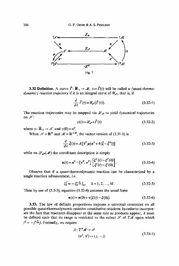
250 G.F. OSTER & A. S. PERELSON
T, .~ T,.,~
~ X 9 A/ A
r ~ " r -2e *
Fig. 7
3.32 Definition. A curve F: ~,+ --* d/ , t ~ F(t) will be called a (quasi-thermo- dynamic) reaction trajectory if it is an integral curve of adno, that is, if
d@/~(t) =~no(F(t)). (3.32-1)
The reaction trajectories may be mapped via .Ea,o to yield dynamical trajectories on ~r :
y(t) = ia.o o/~(t) (3.32-2)
where y: ~.+ ~ / " and y(0)=n ~ When X = R N and ~g=lR 2u, the vector version of (3.31-1) is
d ^ d t r = A [0 r/ t(n ~ + ~(~- ~o))] (3.32-3)
while on ~ .o(Jg) the coordinate description is simply
n ( t ) = n o - [v R, v e] [~: (t) -5 : (0 ) ] (3.32-4) lq'(t)-~'(O)J"
Observe that if a quasi-thermodynamic reaction can be characterized by a single reaction advancement, i . e .
~ = - ~ , ~ ek, k = l , 2 . . . . ,M. (3.32-5)
Then by use of (3.1-3), equation (3.32-4) assumes the usual form
n (t) = n (0) + v (q (t) - ~ (0)). (3.32-6)
3.33. The law of definite proportions imposes a universal constraint on all possible quasi-thermodynamic resistive constitutive relations. In order to incorpor- ate the fact that reactants disappear at the same rate as products appear, A must be defined such that its range is restricted to the subset 06 ~ of T ,g upon which i:= _j,n=j. Formally, we require
A: T * ~ 5 p (~:, ,() ~, (j, _ j ) (3.33-1)
Chemical Reaction Dynamics 251
Clearly, the map (if , j r ) ~ (j, _ j ) establishes 6" as a 2M-dimensional submanifold of the 4M-dimensional tangent space T~r On each fiber, Sa~ = T~dr is a subspace of dimension M. The law of definite proportions thus insures that a single reaction rate characterizes each chemical reaction.
3.34 Remark. In section 4, where we discuss other properties of constitutive relations, it will be seen that the law of definite proportions can be interpreted as an orientation restriction on the constitutive manifold defined by the graph of A in T * . / / x T Jr'.
One need not impose the law of definite proportions as a constitutive constraint. Indeed, as we shall see in Part II, chemical reactions are a subset of a larger class of dynamical systems which are not, in general, so restricted. For example, a more general class of chemical processes might include those in which unknown inter- mediates are present which are not in a quasi-stationary state. For such reactions jY4: __jr. This class of reactions will not be examined here.
3.35. The constitutive constraint embodied in the law of definite proportions restricts the possible trajectories that reactions may follow on ./r to lie on an M-dimensional integral manifold M=../#. To show this, we first construct an M-dimensional (involutive) distribution on ~ . * Let M ' be an M-dimensional manifold. Consider the map
When ~ =IR TM,
~' : ~ - ~ M' ,
(~S, ~,) ~ (~S+ ~,). (3.35-1)
J = [ I~ , IM] (3.35-2)
where l u is the M x M identity matrix. Since the rank of J is M, J is a sub- mersion.
The corresponding tangent map is
Note that
J , : TM[---~ TM',
(jr, jr) ~ ( jr +jr).
kernal ( J . ) = {f~ T.//[ •. j = 0}
= {(H, J ') ~ T~r = - j ' }
= range (A) = 6 a.
(3.35-3)
(3.35-4)
The function A defined by ~ kernel ( J * ~) is an integrable distribution on ./r with dimension M (BRICKELL & CLARK, 1970, p. 194). By the Frobenius theo-
'* A p-dimensional distribution (or p-vector field) on a 2M-dimensional manifold .At' is a function /X on .ar such that for each x in o~': (1) A(x) is a p-dimensional subspace of Tx~r and (2) there is a neighborhood r x on which there exist vector fields X~ .... Xp such that Z~ (m) is spanned by Xlm .... Xpm for all points m~q/(BRICKELL & CLARK, 1970, p. 193).

252 G.F. OSrER & A. S. PERELSON
M
N i
F ig . 8
-- i {~) c.//4
l i M I t MxM (~,-~)
rem, through each point ~ in eft' there passes an M-dimensional integral manifold of A.*
By construction, the vector field ~/no lies in the distribution A generated by A. Therefore, for each choice of initial condition ~(0), the integral curve ~(t) for ~/,o lies in an integral manifold of A. With no loss of generality we set ~ ( 0 ) - 0 and denote the corresponding integral manifold, ~/.
Note that we have a global characterization of h?4 via the natural injection i: NI-~ .~, i.e. the M-dimensional antidiagonal submanifold of .~ :
On ~/, only a single advancement characterizes each reaction. Therefore, we can denote points on ~ / b y ~ with coordinates ~k= i,~Yk= --i,~,k. Since the thermo- dynamic reaction manifold M is also M-dimensional, we can identify M g M by first embedding M ~ M x M via the antidiagonal map i : ~ ~(~, -~ ) . Then, recalling equations (3.32-4) to (3.32-6), we identify ~ : = - ~ ' g ~ and so identify i ( M) with i(~/). In fact, viewing i as a diffeomorphism onto M, we can identify M with J~/ itself: ~ g ~ g (~, - ~) ~ (~/', - ~f) ~ ( - - ~ r , ~ 9 " These identifications are summarized in the commutative diagram of Fig. 8.
It is important to realize that reaction trajectories are confined to .~/ and that a single reaction rate j = y = - j" characterizes each reaction. However, two independent affinities are still required to characterize the driving force for each reaction. Thus
A: T*J[ ~ i.(T~I),~TM,
and the vector field (a:, o:) ~ (j, - j) ,~j, (3.35-9)
~/no = A o - L#* #o L#no (3.35-10)
may be restricted to l~/, yielding the equations of motion
= A o - ~ * #o s (~) (3.35-11)
=A o dG(~)---a ~r (~) (3.35-12)
* A submanifold )kr of .#/is an integral manifoM of a distribution A on J ff for each xE)lT/, A(x)=i.(TxdCd), where i: 217/.-..//is the natural injection (BRIcV~LL & CLARK, 1970, p. 198). Thus an integral manifold is a submanffold whose tangent spaces c o i n c i d e w i t h the subspaces determined by the distribution. By a suitable coordinate change an integral manifold can always be expressed (locally) as the level set x M + 1 = constant . . . . . xa M= constant.
Chemical Reaction Dynamics 253
where (~=i*f#: l~/--+ IR and ~o=~ ~/,ol~. The vector field ~,o yields the equation of motion of a quasi-thermodynamic chemical reaction system when the law of definite proportions is imposed as a constitutive constraint. The whole purpose of this construction was to permit a broadened definition of the affinity covector field while maintaining the kinematic constraints of the law of definite proportions.
3.36 Remark. For stoichiometrically dependent reaction sets we follow a procedure similar to that outlined in section 3.20. Reaction trajectories beginning at ~(0)=0 are confined t o / ~ / f o r all t e ~ + . If t2NM has only r<M independent reactions, the image of M under .o~e,o will be an r-dimensional submanifold of ~ ;
= ~,, to which the motion will be restricted. The submanifold ~ is determined solely by the reaction stoichiometry and is precisely the same as in the thermo- dynamic case. Here, the vector version is given by
- [ v ,v ] = n ~
The vector field ~r can also be transferred to ~ by defining the map .~a~'o: J( / - , such that .oqe~o 1~ = i~ o .~a-o, where i~ is the natural injection, i~: ~ ,--~ ~.. Then, on ~ , we have the vector field X~=L~'~,oAo -.o~e*/lo is~: ~ T ~ .
3.37 Remark. For the reaction set A + B~C, 2C~--D +B, the stoichiometric matrices are
R 1 e 0 v = and v = . (3.37-1)
We assume the capacitive consitutive relation p is an ideal dilute solution and that the resistive constitutive relation A is given by mass-action (see section 4.22); i.e.
[e~f/Rr _ e~'m r] [~ik]=Ak(~fk,~'k)=XkL_e,S/Rr +e,,/Rrj (3.37-2)
where N
and k~ is the forward rate constant for the k th reaction and A~ denotes the k ta component of A. Then inserting equations (3.23-2) and (3.29-2) into (3.35-11) yields the vector field restricted to _~/:
r = ~1 ( /<7 + v - 2 (no _ r (n ~ - ~1 + r - v - 1 (no + ~1 - 2 ~)), (3.37-3)
r = ~ (/<~" + v - 2 ( n ~ + ~ 1 - 2 ~ . ) ~ - v - ~ ( n ~ + ~ 2 ) ( n ~ 1 + ~ ) )
where K~q and K~q are given by equation (3.23-5).
3.38 Remark. There is a superficial resemblance between the vector field 03t~, and Hamiltonian vector fields. As is well known, Hamiltonian flows are pure
254 G.F. OSTER ,r162 A. S. PERELSON
symplectic, of the form
k.J a=- lH
(LOOMI$ & STERNBERG, 1968, p. 521) where H is the Hamiltonian and f2= dp~ ^ dq i. Or, in vector form on R2 ,, i = j VH(x) where
x = ( q , p ) r and j = [ _ O ~ ]
is the coordinate form of I2. Similarly, on R2 m the vector field ~162 has the form
r = A o VG(~).
The two would be identical if A were the linear map J ; the replacement of A by J has an amusing circuit theoretic interpretation which will be apparent in Part II.
3.39 Remark. We wish to thank Professor R. HERMANN for pointing out that the construction of ~ is related to the geometric procedure of generating vector fields on a manifold, tiC, from the module of real-valued functions on ~ ' , ~-(~ ' ) . The two most common examples of this are the gradient and Hamiltonian vector fields: given a real valued potential ~o: ~ ' ~ IR, one obtains a covector field on d[ from dtp. If ~ ' is a Riemannian manifold, then dq~ may be converted into a vector field, grad tp, by the usual isomorphism between T*.#g and Trig' induced by the inner product structure (BIsHoP & GOLDBERG, 1968). In the case of Hamiltonian vector fields, the manifold ~ is symplectic, and therefore carries the canonical 2-form f 2 = ~ dpi A dq i, which can be employed to relate dip to a vector field by contraction: g_l t 2 = - d~o. In the case of the reaction vector field, the free energy function on JV generates a vector field ~ on another manifold ~ ' , via the stoichiometry, where the constitutive relation A ( ' ) takes the place of a Rie- mannian or symplectic structure.
3.40. The equations of motion are subject to the constraint that mass is conserved in each reaction. This constraint is incorporated in the map ~,,o by the following restriction on the construction of the stoichiometric matrix v.
Define a covector field og~T*./Vsuch that (co,, z~)=0, Vz~ET,~where 09 is a constant covector with components equal to the molecular weights w i of each chemical species, e.g. q~* (co)= (wl, ..., WN). Therefore
0 = <co., z.> = <co., s (j, _j)r Vj ~ T ~ . (3.40-1) In coordinates,
Consequently,
=wT , vj.
N
O= w r y = ~ WiVik, k = 1 . . . . . M. i = 1
Thus, by construction of -~~ trajectories of ~ , (~ ,o ) in ~ obey mass conser- vation.
(3.40-2)

Chemical Reaction Dynamics 255
T . ~ = TM
" I 1 k~o , g = . g
Fig. 9
3.41. Avls (1965) has taken as the primitive information for constructing a chemical system a set of atomic species. This point of view may be incorporated into the present treatment by defining another differentiable manifold, d , equipped with a global atlas ~0~,: d - * l R A, a ~ (al , . . . , aa), where A is the total number of elements or atomic species in the system under discussion and a~ is the number of moles of atomic species i. A molecular species can be decomposed into its elements under a linear map, fl: .A/--* d . The matrix representation of fl has (i,j)th element equal to the number of moles of element i in one mole of molecular species j . Since atomic species are conserved in a reaction, we say that a reaction is balanced if f l * o L . ( j ) = 0 Yjr i.e. if every reaction ratejeTM is mapped to the zero vector in T ~ (cf. Fig. 9). The reaction N H 4 O H = N H a + H z O is balanced, L . = v = [1 - 1 0] T and
[! i]1110~ �89 L o J LOJ
while the reaction N H 4 0 H = 2 NH34- H2 0 is not. In the quasi-thermodynamic
case a reaction is balanced if t , L#, (__Jj) =0.
3.41 Remark. t , o L , = 0 places a constraint on the possible choices of the stoichiometric matrix v.
3.42 Remark. The maximum rank of v for a set of balanced reactions is N - A', where A' = rank fl (Ares, 1965). (Since /~: IR N ~ R a and rank /~ + nullity p = iV, the dimension of the null space o f / / i s N - A ' . Therefore, for a balanced set of reactions, maximum rank v=N-A ' . )
4. Constitutive Relations
4.1. In the geometrical structure outlined in sections 2 and 3, chemical reactions have been treated as a separate mathematical object distinct from the species which partake in the reaction. This is a mathematical artifice that allows us to view the properties of the reaction process apart from the equilibrium properties of the chemical system. Implicit in this separation is the assumption that at each instant during the progress of the reaction a unique chemical potential covector can be

256 G.F. OSTER c~; A. S. PERELSON
assigned to the instantaneous species composition. Moreover, at chemical equili- brium, this covector corresponds to the usual thermostatic chemical potentials.*
In this section we briefly comment on a number of physically motivated constitutive assumptions, i.e. restrictions on the form of the maps/a, 2 and A. A more detailed analysis of the effects of these assumptions on the reaction dynamics will be presented elsewhere.
An obvious physical requirement of our model is that out of all equilibrium points of the vector field Sv.~ there be but one that corresponds to the usual notion of thermodynamic equilibrium. In order to insure this requirement and to incorporate the limitations implied by the second law of thermodynamics, we introduce restrictions on the admissible constitutive relations.
4.2. Most of the results to be presented in this section apply to both the thermo- dynamic and quasi-thermodynamic reaction constitutive relations. Therefore, we shall generally state results in terms of the quasi-thermodynamic construction; the thermodynamic case will follow mutatis mutandis except as noted. We shall assume throughout that the law of definite proportions holds and state many of our results on the manifold h5/.
In conformity with this general philosophy we shall define thermodynamic equilibrium in terms of the quasi-thermodynamic affinity. We then show that our definition is equivalent to the usual thermodynamic definition: a = 0.
M
4.3 Definition. A reaction set g2nu at advancement ~eM is said to be in a state of thermodynamic equilibrium if
(i* ~)~= 0
where i: M - + . / / is the natural injection.
4.4 Proposition. A reaction set Onu described by a thermodynamic reaction constitutive relation at advancement ~ e M is in a state of equilibrium if and only if ar = O.
Proof. Let i: J~4 ,--.Me be the natural injection, and let i(~)=~, ~e/~/, ~ e J 4 ; then ~ = ( J , a')~
M M
ak(O d ~ . k = l k = l
Pulling ~ back along i (i.e. imposing the law of definite proportions), we have
M M
O* ~)~= Z a[o i(~)d(C~o 0~+ Z ~;o ~(r '~o i)~ k = l k = l
M
k = l M
k = l
* This assumption is related to the "local equilibrium" postulate of continuum mechanics. That is, we require only that the capaeitative constitutive relation #(n) be unique and identical at each instant with the equilibrium quantity corresponding to the instantaneous composition.

Chemical Reaction Dynamics 257
By the identifications of Figure 8,
M M f , E
k = l k = l
Therefore (i* ~ ) ~ ~r
4 .5 Remark . W h e n ~ = ~ 2 M, _~/= IR~ = M and
Also observe that M
k = l
thus if ~ M is a state of thermodynamic equilibrium, C~k(~)=0, k = 1, 2 . . . . , M. If only r < M reactions in f2NM are independent, then each ~k, k = r + l . . . . , M may be expressed as a linear combination of the independent reaction affinities a l , . . . , a,. Consequently, a reaction set s at advancement ~ with r independent reactions is in a state of thermodynamic equilibrium if and only if ak(~)=0, k = l , 2, . . . , r.
4.6 Definition. The equilibrium submanifold, ~ , of a reaction set ONM is the set of points ~ e M at which the pull-back of the thermodynamic affinity vanishes:
This corresponds in the thermodynamic case to the submanifold
4.7 Remark. If/~ is exact, then we haveL* G: M ~ ]P,, such that ar = d ( - L * G)r (cf. section 3.13). CM is the critical set of L*G. Similarly, the critical set of i * ( - - ~ * G ) : -~/--~ ~ is r
4.8. For discussing the restrictions on the resistive constitutive relation, it will prove convenient to adopt the following viewpoint. Let the graph of A: T * . / t ' ~ T ~ / b e denoted by A~:
Ag =~ {(~, j') e T*.~' x T~Cr
It is well known that A s is then a closed submanifold of T*J#• (e.g. DmUDOr~N~, 1972, p. 48). For a single quasi-thermodynamic reaction Ag is a two- dimensional submanifold of R 4, while for a single thermodynamic reaction 2g is a one-dimensional submanifold of R2. * A point peA s is called an operating point. The graph of the incremental constitutive relation, A : , at an operating point p is the vector subspace TpA s of T(g,a(~))(T*J[ • Tall), i.e. the tangent space of Ag at p. Note that since TpA~ is a vector space, we can define the (Euclidean) inner product srt of any two vectors s and t in TpAg. Constitutive assumptions
�9 Since A is a constraint only on the fibers, we can ignore the base point ~ and consider the graph of A acting on the second factor only.
18a Arch. Rat. Mech. Anal., Vol. 55

258 G . F . OSTER • A. S. PERELSON
will be discussed in terms of the shape and orientation of A~ and TpA~ in T *.ll x T.//[.
4.9 Definition. The dissipation associated with a reaction set is a real-valued function on J / , # : ~ ~ , defined by evaluating ~ on the tangent vector A(a) at each point ~ed/ ,
M M
= E =~(')J~(')+ E =;(')J;((') k= l k= l
where ((~, 7) ~ Ag. Observe that whenj is restricted, by the law of definiteproportions j = (j, - j ) and
M
/r
Pulling # back to/~/, we define the dissipation as
M (~(i*~)(~)= ~ (~[--~;,)o i(~)jko i(~).
k = l
By the identifications of Figure 8 the dissipation due to thermodynamic and quasi-thermodynamic reaction constitutive relations constrained by the law of definite proportions is the same.
4.10 Definition. The reaction constitutive relationA is called passive if ((t, 3) > 0 for all (~,~)~Ag and strictly passive if ( ~ , ~ ) > 0 for all (~ ,~)#(0 , 0). A passive constitutive relation has non-negative dissipation, i.e. ~ : ~r162 ~ + . A constitutive relation is called active if it is not passive.
4.11. The reaction constitutive relation A is called locally passive at a point peAg if 5gTtsj>O V(fi~, r3j)~TpAg. If there exists a single pair (t~, 3j)~TpAg such that c5 ~rtSj < 0, then A is called locally active at p. The constitutive relation A is called locally passive if it is locally passive at all operating points. However, it is customary to call a constitutive relation locally active if it is locally active at any operating point.
4.12 Remark. Note that a reaction constitutive relation may be passive and not locally passive, or locally passive and not passive; cf. 4.23 to 4.26.
4.13 Prolmsition. Given a C 1 map A : ~.J--} ]R t, the following are equivalent: (1) A(.) is locally passive. (2) Da(x)_>__0, v x~]R'. (3) [A(xl)-A(x2)] r [ x l - x z ] > 0 , i.e. A is monotone. A map having this
property is sometimes called "dissipative."
Proof. (1) and (2) are equivalent by definition of local passivity. (2) and (3) are equivalent; cf. ORTEGA • RHEINHOLDT (1970), p. 142.

Chemical Reaction Dynamics 259
4.14 Theorem. I f A is passive and it is exact, then for any reaction trajectory F: ~,---,.r162 there exists real-valued functions fg: .1r ~ ]P, and G: .A/'---, ]P, such that a dG
ff>O along F and--d-i- < O along .WnoF. dt -
ProoL Since/~ is exact, there exists a real-valued function G: vf ~--, ~, such that # = dG. Therefore ~ = - .W*/t = d&, where @ = - .W* G. By hypothesis (~,) ' ) r (o > 0 and therefore
- d (dfa(r ~)r(o = -d7 ~ o r____ o
for all points ~ on F(t). Moreover since
d ~=- .v*~= -Go.o , -dTGo~noOr=<0.
4.15 Remark. The irreversibility condit ions/ , rh < 0 used by KRAMBECK (1970) is equivalent to our passivity assumption. The passivity condition on A therefore encompasses the restrictions on q/no(') implied by the second law of thermodyna- mics. Passivity, as we show below, is also a sufficient criterion for having all reaction rates vanish at thermodynamic equilibrium. Consequently, it also includes constraints usually ascribed to the principle of detailed balance.
Detailed balance at equilibrium, or the " law of entire equilibrium", as G. N. LEwm (1925) first expressed it, requires that every elementary process have a reverse process and that in a state of equilibrium the average rates of the for- ward and reverse processes be equal. Here we do not restrict ourselves to "separ- able" constitutive laws in which the reaction rate can be written as the difference between a forward and reverse rate, and thus we ascribe to the law of detailed balance only the fact that in a state of thermodynamic equilibrium each reaction rate vanishes, Le.j~=O for all k = 1 . . . . . M.
4.16 Theorem. I f A(') is passive and obeys the law of definite proportions, then . . . . A
all reaction rates j ~ = A( ~ ) vanish along the equdtbrmm submanif oM ~ = i ( r ).
~$k_,~rk and j~ is the equilibrium reaction rate ProoL Let ~err~=dt ' . Then ~ - ~ which we will show equals zero. Let s e T * d / h a v e only one non-zero component; say the first, such that_~'= el (~) d~ 1, where el (~)>0 is constant for all points ~ in a neighborhood q /o f ~. Letj~" andjb ~" be the reaction flows given by (j'~, -j~)~ = A(~+e~)A=A(6tLr162 ~) and (Jb, - -Jb)~=A(~ - r" zx_, f ,. ~ ) = . a ( ~ - e~, a~), respectively, V ~eq/. The dissipation ~o associated with the pair {(Ja,~'J,)~, A(a~+e~, a[)} for all ~eq/is ~ ( ~ ) = ((a~+ e~, ce~), (./'~, --jo)) = (e'~,j~$) = ~l (r ( J~) l , where (J'~)l
M
is the first component of j ~ ! = ~ ( j~) f 8/d~il~. Similarly, #b(~), the dissipation i = 1
associated with the pair {(Jb, --Jb)~, A ( ~ - - e~, c~)} is given by #b (~) = ( -- e~, Jb ~) = - -~(~) ( j~)~ V ~eq/ where (j~')l denotes the first component ofjbi . Since A is passive, # , (~) = e~ (~) (jo ~) t > 0 and #b (~) = - el (~) (Jb ~)~ > 0. Consequently (jo ~)~ > 0 and (j~ ~)~ < 0 V ~eq/. However, since A is continuous, as e~ (~) -o 0, (Jo0t and (Jb~)~ smoothly approach (ff~)l, the first component of ~ . Hence (~)~ must be zero. Similarly, all components of ]~= 0.

260 G.F. OSTER & A. S. PER~LSON
K.RAMBECK (1970) proved a similar result for the case of mass-action kinetics. Theorem 4.16 is more general; in sections 4.23 and 4.26, for example, we show that the mass-action and Michaelis-Menten constitutive relations are passive.
4.17 Remark. It is interesting to note that to each point ~e~*~ there need not correspond a stationary point on Jff. However, since ~ , is linear, hx, o(~)= La, j~ = 0 at all points n ~ s where 3v" ~ { ~ e i(~/) [j~ = 0}. Passivity insures that g~tc3w and thus to each thermodynamic equilibrium point there corresponds a stationary point on ~..
4.18. In general, there can exist points ~ ~ i(~/) such thatj~ = 0, and yet i* a~ + 0. Such points have been called points of false equilibria (PmGOGINE & DErAY, 1954) and regular equilibrium points by KRAMBECK (1970). However, if we impose the more stringent requirement of strict passivity, then one can show that every point
where ]~ vanishes is in d~ Similar results have previously been stated by COLEMAN & GU~T1N (1967), BOWEN (1968b), DUNWOODY (1969), and KRAMBECK (1970).
4.19 l_emma. I f the reaction constitutive relation A is strictly passive and obeys the law of definite proportions, then for any point "~zi(Yl), ~ = A ( t 0 = 0 / f and only if i* ~ = O.
ProoL At any point ~eJ//, if i * ~ = 0 , ~eg~ and by Theorem4.16, j~=0. Conversely, if at any point ~ei(ff4), A(a~)=0 and i*ct~4:0, then ( a ~ , ~ > = 0 , contradicting strict passivity.
4.20 Remark. We can easily relate the above results to properties of the vector
field. ~,o. In fact, since j~ =~=~,,o(~)=A o (-Aa*#)o L#,o(~)=A(~(~)), points at which ]~ vanish are simply the equilibrium points of the vector field ~,o. Thus the vector field has the characteristic of totally reflecting the properties of the resistive constitutive relation insofar as the determination of its equilibrium points are concerned. The thermostatic constitutive relation/~(-), and the reaction topo- logy, v, only effect the possible values of & and thereby determine thermodynamic equilibrium points. When A is strictly passive, the vector field and thermodynamic equilibrium points coincide.
We can rephrase the above lemma by defining the following sets:
= {~ E z(M) l ;~ = ~ = o},
.~ ~ {~ e i (/15/) [ i*t~ 4= O, and f~ = 0};
is then the set of all vector field equilibria, ~" is the set of false equilibria, and ~" c ~v- c J / . These sets are related to the set of thermodynamic equilibrium points 8~ by
~- = ' U \ ~ g (i.e. ~" =3v'n g~),
where 8~ is the complement of ~./. Therefore we have the following:

Chemical Reaction Dynamics 261
4.21 Proposition. If the reaction constitutive relation A is strictly passive, then (i) there are no false equilibrium points, Le. ~" = 9, (ii) every equilibrium point of the vector field is a thermodynamic equilibrium point, Le. ~e" = d'~.
4.22 Example. Mass-Action Constitutive Relation. For gas phase reactions the mass action constitutive relation has successfully described most experimental information (e.g. PRATT, 1969). Usually the mass-action expression for an elementary reaction is written as a polynomial expression in partial pressures or concentrations, i.e.
1 d~ N = kS I-~ c ~ - k ' I - [ c~ ~ (4.22-1)
V dt i=1 i = i
where V is the system volume, and k s and k' are the forward and reverse rate constants, respectively. Assuming that the system is ideal dilute (equation 2. I0-1), then equation (4.22-1) may be rewritten in the form
j = x I e ~t/Rr- x, e ~'/Rr (4.22-2) where
N
(4.22-3) N
x , ~ V k r e x p [ - - ~ = l V r # p / R T ] > O .
The equilibrium constant Keq is given by
K,q ~- exp [ ~= f v ~ - v~ /tp /R T] . (4.22-4)
4.23 Proposition. A reaction that obeys mass-action is (a) passive if and only if kl/k" = Keq, (b) not locally passive.
Proof. kl
(a) If -~ -= Keq , then Kf = X rlX X and
(uf, ~ )r (j, _ j ) = X(otf _ ~,) ( e a / R r e,,IRT) > 0 k f
for all ~Y and ~'. Hence mass-action is passive. Conversely, if ~-~=Keq, then ir ~= ~c,. Assume x f > x,. Then
( (uf, ~'), (j, - j ) ) = (~f - ~') (~: y e a /Rr - ~:, e ~" /RT ) < 0
for all a s and a" satisfying the inequality: In u s + a f > a" > a I. Thus mass-action is not passive, x,
(b) To test for local passivity at an operating point p, we examine
~ f ~I /RT f ~ Kr ~r/RT r
18b Arch. Rat. Mech. Anal., Vol. 55

262 G.F. OSa'ER & A. S. PERELSON
By the same arguments as used in part (a), mass action is locally passive at the operating point p if and only if
(x s e~1/RZ)e = (X, e~"/Rr)e. (4.23-1)
We assume that mass-action is passive; then ~:y=rc,, so that equation (4.23-1) is satisfied only at operating points where ct s = ct', i.e., at thermodynamic equili- brium. However, even if mass-action is not passive (xy =~ x,), there still exist operat-
ing points where equation (4.23-1) is not satisfied (in fact, at all points p /
where \
~r +. ors + R T In ~_I) ; therefore mass-action is not locally passive. This completes - v T t
the proof.
4.24 Remark. On physical grounds, one should expect that a reaction rate model is passive, since activity would imply the capacity to supply energy inde- finitely. For closed systems of elementary reactions the principle of detailed balance is usually employed to ensure that kf lk ,=Keq. Here we shall directly assume that all reactions that occur in a closed vessel are passive.* (Theorem 4.16 then guarantees that they obey detailed balance.) Consequently, we shall hence- forth employ
j = x (e "'/Rr - e "'/Rr) = A (a s , ~') (4.24-1)
as the mass-action constitutive relation for a reversible elementary reaction. With this constraint, we have shown in the above proposition that mass action is locally active at all non-equilibrium operating points.
4.25 Remark. FEINBERG (1972) has coined the term "Marcelin-De Donder kinetics" to describe any reaction that obeys the constitutive relation given by equation (4.24-1), where x is taken to be an arbitrary constant and where ct s and c~' need not correspond to the actual affinities of an elementary reaction. The above proposition shows that the Marcelin-De Donder constitutive relation is passive but not locally passive. From Theorem 4.16 we conclude that Marcelin- De Donder kinetics exhibit detailed balance. A somewhat similar result has previ- ously been established by FEINBERG (1972).
4.26. The situation concerning mass-action is not quite as simple as it appears. In its most general form, the mass-action constitutive relation is a polynomial function in concentrations or activities. As such it can be viewed as a map n ~ P ( n ) = h, from JV to TJff. Introduction of the stoichiometric constraints on the n~ effectively transfers the dynamical system to ~r r ~ R (~) where R: ~g ~ T~/ is the map completing the commutative diagram in Figure 10: .oq'.o R = P o .~e,,o. Therefore, the mass action kinetic equations effectively prescribe a map Q: J V ~ T~r that R = Q o .Lr p=.LaooQ which replaces the map
(Ao - ~ e * o #o ..~a,o): sV'~ TJ//
* HORN & JACKSON (1972) have relaxed the constraint of detailed balance in order to discuss, within a chemical kinetic framework, more general situations than chemically reacting mixtures in closed systems. Passivity is not expected to hold for such generalized mass-action systems.

Chemical Reaction Dynamics 263
�9 r * X ,,. T* .~ _ ~ -
Fig. 10
(cf. Remark 3.39). Consistancy with thermodynamics necessitates the introduction of an independent constitutive assumption on Q, e.g. detailed balance at equilib- rium. As we have shown, passivity of A replaces detailed balance in our formula- tion.
In order to isolate a resistive constitutive relation A, in equation (4.24-1), from equation (4.22-1), we have to rely on some rather adventitious choices of functional forms. Namely, the ideal dilute solution being an exponential function, n~= Ve (~'-~~ which maps the multiplicative group on IR to the additive group and thereby converts the polynomial to an exponential whose exponent contains a sum of chemical potentials. Moreover, this sum contains the affinities, ~s and ~" providing the exponents in P are just the stoichiometric coefficients. If the thermostatic constitutive relation is not ideal dilute, or, if the reaction order and molecularity do not coincide (APas, 1969, p. 80), then there is no assurance that the constitutive relation j = A(~ f, ~') could be filtered out of equation (4.22-1). For reactions which do not represent elementary steps or for heterogeneous reactions, one frequently writes (ARIS, 1969, p. 60)
R (~) =f(~) I'k; H(e ~ + vj ~)PJ- k" 17 (c ~ + v i ~)v,]
where f ( ' ) is a positive function, and flj and 7j are arbitrary real numbers. It can be shown that to be consistent with thermostatics one must have n vj = 7 j - fl~ and Kgq=kY/k" where n is a positive real number (DENeIGU, 1971, pp. 444--445; Bt.UM & LUSS, 1964). However, we proposed that, rather than patching up a dubious reaction rate expression, it is probably better simply to perform measure- ments of reaction rate as a function of forward and reverse affinities, ~ = A(~ y, ~'), and be assured that A passive will ensure consistency with thermostatics. It is probably important to emphasize that measurement of A involves only steady state experiments. Construction of the vector field ~/,o thus, in principle, involves only equilibrium and steady state experiments, separately performed; dynamic (e.g. relaxation) experiments are only required for reaction systems where each reaction cannot be examined separately.
Finally, it can be shown that the vector field P (or Q) will maintain all concen- dR
trations in the positive orthant andthat for non-autocatalytic reactions --d-( < 0,i.e.,

264 G . F . OSTER & A. S. PERELSON
the reaction rate decreases as one approaches equilibrium (ARIs, 1969). In the present theory the former requirement is ensured since we have modelled JV on RN+ ; the latter will be shown in section 4.30.
4.27 Example. Miehaelis-Menten Constitutive Relation. In many instances, the enzyme catalyzed reaction S ~ P may be described by the simple mechanism
kt ka 8 + 6r , ~ g S ~.~ g + ~. (4.27-1)
k2 k4
When the initial concentration of substrate greatly exceeds the total concentration of enzyme, Cso >> CEo, the Michaelis-Menten constitutive relation
_ KM cs-- V~t KM Cp (4.27-2) V dt s , r s KMKM+KMcs+KMCp
is applicable. The maximum velocity for the reaction S ~ P is V~= k 3 Ceo, and its
Michaelis constant K~ = kz + k3. For the reverse reaction P ~ S, V~ = k2 CEo and k2 + k3 kl
K ~ = - - k ,
In the derivation of the Michaelis-Menten equation (cf HALDA~rE, 1930, p. 40) the pseudo-stationary-state hypothesis is applied to the enzyme-substrate complex,
d i.e. one assumes ~ CEs=O. This assumption may be seen to be valid in the limit
C~o/Cso--* 0 by the use of singular perturbation techniques (HEINKEN, TSUCHIYA &; ARm, 1967). However, since
0 = d 1 �9 dt Cr's=--# (~x - ~2) =F(r ~z),
the non-linear constraint
0 = F (~ 1, ~2) = k l (CEo - - ~ 1 + ~2) (Cso -- r 1) - - (/62 + ka) (~ x - ~2) '[- k, r (%0 - r x + ~2)
(4.27-3)
is imposed on the reaction advancements, where we have employed the fact that
~l=kl(C~o-G +~2)(C~o-~1)-k2(~1-~), ~2 = k3 (r - r kh ~2 (CEo -- ~1 + ~2) (4.27-4)
are the rates of the reactions E+ S,-~-ES and E S ~ E + P, respectively. By the implicit function theorem, if OF/O r # 0, then locally one can express the constraint (4.27-3) as ~2=g(r or, if aF/O~l#:O (4.27-3) can be expressed as r =f(~2). It is easy to see that one of these two forms exists at almost all points (~1, ~2) and that locally, at least, the total enzymic process may be described in terms of a single reaction advancement.* However, since both OF/a~ 1 and OF/O~2 are zero at some points (~1, ~2), the conditions of the global implicit function theorem (KuH & HAJJ, 1971)
�9 In fact, if k l=k 4, then one of the two forms exists at all points. If kld6k4, then there exists a single point where OF/O~I = 0 and OF/a~2= 0 and neither form exists at that point.
Chemical Reaction Dynamics 265
are not satisfied. Consequently, a global coordinate system cannot be found to describe the constraint surface and a manifold formulation is essential. We shall comment on this point further in Part II.
The reversible Michaelis-Menten constitutive equation (4.27-2) may be ex- pressed in terms of the forward and reverse affinities of the overall reaction S ~ P . Assuming the solution is ideal dilute, we have
~f = p s = l ~ + R T In c s,
o~'=lZe=#De + RT lnce .
Solving for c s and c e and substituting into equation (4.27-2) yields
1 . e ~t/Rr - - e ~ ' I R T
(4.27-5) --V J= e ~'/RT ~-e ~'IRT K ~ e~llRr
where the thermodynamic constraint
V~ K'~ (4.27-6) I~ms -/tme = R T l n K e q = R T l n V~ K ~
has been used. The law of definite proportions then requires j = ( j , - j ) , and A: (c~ y, c~ 0 ~)" is thus determined by (4.27-5).
The structure of the Michaelis-Menten equation is the same as is shown in Figure I0, but now P, Q and R are rational rather than polynomial functions. Once again, the isolation of A from R depends on the fortuitous invertibility of the map e ~ (~s, ~).
4.28 Proposition. The reversible Michaelis-Menten constitutive relation is passive and locally active.
Proof.
R T
V(~ I ~,j(e~t/Rr~ _ e~./~T) >-- 0 V OJ, O~ ~,
c, 4- c, " [ - z x M eltns/RT - T--;Tr--
r M V M r M
1 1
[_._~M e~I/RT e ~ +----r +
v~ j
K M ~ /Rr 2 e ] NO.
4.29. Thermostatic Constitutive Relations. The usual thermostatic constitutive assumptions may be applied to the map/z(.). For example, there is the thermo-

266 G . F . OSTER 86 A. S. PERELSON
static stability condition, D/~> 0, for all n e ]RN + . We have previously introduced the ideal dilute solution constitutive relation (cf. 2.10-1). In general, for ideal gases, ideal solutions and solutions obeying Henry's law/~i is a logarithmic function of the composition variable ( p i ( n ) ~ R T l n n i ) , implying / ~ i ( n ) ~ - ~ as n i ~ 0 . KRAMBECK (1970) has previously argued that this asymptotic behavior plus passiv- ity is a sufficient condition for keeping all composition vectors in the positive orthant. As a consequence of thermostatic stability we have the following.
4.30 Proposition. For non-autocatalytic reactions obeying mass action and ideal dilute solution constitutive relations, Oj/O ~ < O.
Proof. ] = A(a), i . e . , j = j ( O t f , o~r).
Therefore aj tgj r ~f ~ ]'/l ~ nj t- ~ dj act' t~/z i d ny r --i~,j ~0~ f (~l.ti (~nj ~ __',y (~o~" (~l~ (~ny ~ "
Assuming mass-action, we have
aj ~ T ~3j x a~ J' = e~S/Rr' d~ ~ - R---T e~'/RT ;
~j x ~. r..~s/Rr. R . . . . . ~./RT e ,, �9 - - L ~, v i I ~ i j r j - - ~ v i i ~ i j Vj]. " ~ R T i, j
We assume the solution is ideal dilute
Oj x 0 r - R T ~ #" [e~t/'r v~ ( - v~ + v P) - e ~r/R r vP ( _ v~ + v/P)].
If the reaction is not autocatalytic, each species is either a reactant or a product in each reaction; therefore,
dj x d r = R T/~/~i, [ - (v~) 2 e"/RT-- (V/P) 2 e"/RT]
- - R T ~i [(V~)21ziie~'/RT +(v/P)2 #"e"/'T]<o=
since by thermostatic stability / t ,>0 . The equality holds only during a phase transition, e.g. precipitation reaction�9
4.31 Reciprocity. In any formalism, the choice of primitive assumptions is usually a matter of taste and convenience. In section 2.11 the differential form #: JV~ T* JV was assumed to be exact, i z = dG, where G: ~r ]R is the free energy. The Poincar6 Lemma, do dG=O is then equivalent to the Maxwell reciprocity relations, i.e. D2G (n) = D 2 G (n)r.
Conversely, one could as easily view this reciprocity condition as a constitutive assumption on the n-port capacitance represented by/~, albeit one which applies to all known materials since it is equivalent to the existence of a unique potential

Chemical Reaction Dynamics 267
function which characterizes the equilibrium state.* The question of reciprocity applies as well to the resistive constitutive map A; that is, when does DA = D A r ? If we assume that chemical reactions are always uncoupled, in the thermodynamic case, this is sufficient to assure that 2 is reciprocal. The area under the constitutive curve can be used as a potential for each entry in the diagonal matrix 2 (MILLAR, 1951 ; OSTER, PEI~a~LSON & KATCHALSKY, 1973). In the quasi-thermodynamic case, however, reciprocity is an additional hypothesis on A whose validity must be determined experimentally, or deduced from statistical mechanics. Nonlinear irreversible processes are often non-reciprocal (cf ROSENBROCK, 1962). Conse- quently, resistive constitutive relations cannot, in general, be characterized by potential functions. In the case of chemical reactions, there is certainly no reason to assume reciprocity. In fact, as we shall see, the law of definite proportions may be incompatible with reciprocity except at equilibrium.
4.32 Proposition. The mass action constitutive relation (4.22-2) is only reciprocal at thermodynamic equilibrium.
Proof. f r l(. [ e af/RT - e ~'mr]
OA(~,~ )=--RY [_e~S/Rr e~rmr ] #OA(af,~') r unless ~ f = ~r.
In the neighborhood of thermodynamic equilibrium ONSAG~R has argued, and experiments have born out in many instances, that resistive constitutive relations are reciprocal. Reciprocity of A at equilibrium is thus another physically reasonable constitutive constraint. If this equilibrium behavior is postulated, then A, when linearized about a thermodynamic equilibrium point p, reduces to 2. That is, if i*~p=0, then DA (~tp) is a quasi-diagonal block matrix
0 DA (~I')= [DA ~6~I! . .DAM(&M)] "
The law of definite proportions ensures that Jk = (J~, -Jk) and therefore each block
=
has the form
OA OA 1 dA OA
The postulate of reciprocity at equilibrium then implies
~Jk ~Jk
* In fact, this latter approach to thermostatics was advocated by BR~NSTED in the 1930's. He felt that the introduction of "unmeasurable quantities", such as free energies, was artificial and unnecessary (LAMER et al., 1949). Of course, the equilibrium conditions can be calculated as well using only the constitutive relation, conservation of thermodynamic displacements and continuity of potentials. However, the extremal formulations of Gi]ms are always available since the equilibrium constitutive relations are always reciprocal (OsTeR, PERt~LSON & KATCHALSKY, 1971, 1973),
268 G.F. OSTER &; A. S. PERELSON
and hence
the incremental constitutive relation for each reaction is a 2 x 2 matrix with four identical entries (modulo sign). This entry can then be used as the scalar constitutive relation, 2k" This assures that, about chemical equilibrium, the thermodynamic affinity, - ~ r i p , characterizes the reaction, in accordance with the classical treatment.
4.33 Remark. BRAVTON has given an interesting and useful characterization of reciprocity. Since the reaction constitutive relation (~, 4 ) ~ (~, A(~))= (~, 3) is a map between the second factors (a fiber map), it can be viewed as a submanifold A, of ]p4u via the graph of A. Then, analogous to section 2.12, we can define a 2-form on Ag by
2 M
zx ~ d o~ i ̂ dj i pR = 5 = 1
where for i=1 . . . . . M, f i_j f i , cq_~fi and for i = M + I .... ,2M, jf_j,,i-M, ~i--a,"-M. The vanishing of PR on TAg can be taken as the definition of reciprocity. A simple computation shows that p R = O is equivalent to the symmetry of the Jacobian of A:
M 2 M (aA, C~Ak ) ~. do~iAdj i= ~, ~, d~kAdoti=O.
i = , i = 1 k < i t~ O~ k t~ O: i
The concept of reciprocity turns up in various contexts throughout physics, e.g. Maxwell relations in thermostatics, Onsager relations in thermodynamics, canonical transformation theory in mechanics, and network reciprocity in circuit theory. There is an abstract connection between reciprocity and the geometric notion of a "Lagrangian submanifold" which unifies all of its various applications. The underlying common denominator is the ubiquitous occurrence of "conjugate variables" in many physical theories (e.g. position-momentum, pressure-volume, current-voltage). In the light of our previous discussions, it is clear that this notion of conjugate variables (or " th rough" and "across" variables, as they are known in engineering; MACFARLANE (1970)) corresponds mathematically to coordinates on a space and its dual. Roughly, the connection between the various forms of reciprocity may be explained as follows (for details, see ROELS & WE1N- STEIN, 1971; DESOER 86 OSTER, 1973):
Given an n-dimensional vector space, V, consider the linear space ~ = V x V*, where V* is the dual of V, with coordinates on ~f(x 1, ..., x", y , , ..., y,). By considering V to be the tangent space TpM at a point, p, of a differentiable mani- fold, M, we can extend the following considerations pointwise to the manifold case. ~ has even dimension 2n and can be equipped with a non-degenerate,
n
bilinear form, t2 = ~ dx i ̂ dyi, which is congruent to the skew-symmetric matrix
0 In mechanics, W" arises as the cotangent space at a point of the J = - I , "
"configuration space" of the system: xf=positions, y i=momenta . The cotangent
Chemical Reaction Dynamics 269
space always carries such a canonical symplectic structure which is used to generate the equations of motion (cf. section 3.38). There is a distinguished class of sub- spaces of ~ , called Lagrangian subspaces, which are defined by the vanishing of the 2-form f2; i.e. if s, t are vectors in ~,, then f2(s, t)=srJt=O defines a Lagrangian subspace (analogous to the quadratic surfaces defined by the level sets of a symmetric bilinear form)*. Generalizing, a Lagrangian submanifold, M ~ x 2n, is characterized by the vanishing of the 2-form f2 at each point, p~M, i.e. g2p(U, v)=0, for all tangent vectors u, vrTpM. Thus, each tangent space of a Lagrangian submanifold is a Lagrangian subspace.
The connection between this construction and reciprocity arises when the coordinates x ~ and y~ are functionally related. This occurs, for example, when the x i and y~ are employed as "input-output" variables, measuring the constitutive response of some physical system: y=F(x). The condition that the system be reciprocal (i.e. symmetric under exchange of small signal input-output perturba- tions) is that the submanifold defined by the graph of F( ' ) be Lagrangian. That is, if
S = , t = !1 V
are two tangent vectors to the manifold M at the point p= F(x , then
O=f2,(s,t)=(~=dxiAdyi) (s, t),
= ~ {dxi(s) dyi(t)- dxi(t) dyt(s)} i = l
= Y, {u, [DF(p) ~ ] , - ~, [DF(p) ~],} /=1
= u ~ [Dr (p) v ] - [DF(p) ~]r~
= U ~ [DF (p)-- DF(p) ~] v o r
=if . I t .
Thus, DF(') is symmetric when the graph of F( ' ) is a Lagrangian submanifold. That this imposes rather stringent orientation requirements on the submanifold defined by F (') can be seen by noting that the 2-form t2 ( . , . ) measures the (oriented) area of the 2-dimensional parallelogram spanned by the tangent vectors s and t. Thus the requirement that t2 annihilates pairs of tangent vectors means that the sum of the projections of this parallelogram on the coordinate ("constitutive") planes (x l, Yi) must exactly cancel.
As mentioned above, only transformations of the embedding space which leave the form I2 invariant will preserve the property of reciprocity. That is, if T is a coordinate change on qr
z-- Tz
* srjt is just the Lagrange bracket from classical mechanics; hence the terminology.
270 G.F. OS~R & A. S. P~Rr_~SON
where z = | ~ | , then s ~ t will hold in the new coordinates if and only if i..,pv J
T T j T = J
i.e., if T is symplectic (these are the canonical transformations of classical me- chanics.)
Viewing the reaction constitutive relation in this light, we can see that the law of definite proportions, which requires that j [ = - j ; also imposes an orientation restriction on Ag, one that is not compatible with reciprocity except in the thermo- dynamic case.
4.34. Let us briefly examine the vector space equations of motion linearized about an operating point under the reciprocity assumption. Variables x~ evaluated at the operating point will be denoted 2~.
61t= - ODA (~) ~ r D tt(n) j n
where n = n ( 0 ) + r 6 n = n - n and
~=n(O)+~
is the operating point composition.
If we assume D A ~ ) = DA(~-) r, then the equations of motion assume the form
~ h = A . B fin where A a=-~DA(~)~r=A r and DZG(n)=B=B r since D/ t (n)= D2G(g). If the reactants are sufficiently dilute, the diagonal ideal solution con-
R T stitutive relation may be employed, (B)ij=~-j-.6ij. Then B commutes with A,
and the vector field AB = (AB) r. In this case, the vector field is a gradient flow and the relaxation modes to equilibrium are characterized by real eigenvalues only (WILLEMS, 1972; MEIXr~ER, 1964). Near equilibrium, where one generally assumes reciprocity, the above is a well known result in non-equilibrium thermodynamics. Note that reciprocity provides a potential, while other assumptions, including passivity, are needed to determine if this potential can be used as a Liapunov function (cf. BRAYTON & MOSER, 1964).
4.35 Definition. A constitutive relation j = A ( ~ ) is said to be bilateral if - ~ = A(-~) . If ~ is a function of~ s alone (e.g. Oj/Oct'=O), the constitutive relation is said to be unilateral
A completely irreversible reaction is characterized by a unilateral constitutive relation, since there is no "back effect" of the product concentration on the reaction rate: a unilateral reaction constitutive relation acts as an ideal "rectifier".
In the thermodynamic case, bilateralness is simply anti-symmetry of the constitutive curve about the j axis. A glance at the mass action constitutive relation j = x(e ~I/RT- e ' 'mr) shows that it is not bilateral. FRAZIER & ULANOWICZ (1970) have employed this property of reaction constitutive relations in conjunc- tion with facilitated transport in membranes to analyze a membrane " p u m p " , wherein periodic variations in reactants result in net accumulation of product.
Note that the property of bilateralness is not related to reciprocity. The former is a global symmetry property of the constitutive relation while the latter is a local

Chemical Reaction Dynamics 271
orientation property of its tangent plane. A reciprocal function may be bilateral or not and vice versa. Of course, any linear (or linearized) constitutive relation is bilateral.
It is easy to see that all unilateral resistive constitutive relations are active. In fact, (j, __fit (O~f, ct,)=j(af) (af_a,)<O for a'>a f and j > 0 .
In chemistry irreversible reactions provide examples of unilateral constitutive relations.
4.36 Example. The Michaelis-Menten equation for the irreversible reaction S ~ P may be obtained from equation (4.25-2) by letting k4 ~ 0. In this limit, equation (4.27-2) becomes
1 d~ V~Cs -V dt - K ~ + c s (4.37-1)
and substituting the ideal solution constitutive relation, we obtain
V f eallRT j = V e~t/Rr + K ~ e~/Rr . (4.37-2)
Similar results may be obtained for other types of Michaelis-Menten schemes. For example, the kinetics of enzymes inhibited by excess substrate may be de- scribed by reactions E+ S~ES--* E+ P, ES + S ~ E S 2 with rate law
1 ^ V M c S
--V J = Cs + KM + Ks c 2 (4.37-3)
where K s is the equilibrium constant for the formation of the inactive complex ES2. Again, assuming the solution is ideal dilute yields
-V J = VM/[1 + KM e- (~'- ~)/RT + Ks e (~'-u~')/Rr ].
4.37. If the product concentrations of a reaction are maintained near zero by some means, then the reaction appears irreversible for finite reactant variations. We distinguish such cases from true unllateralness (which is a property of the resistive constitutive relation only, not the operating point) by calling them reactions "far from equilibrium" (ARIs, 1969). Such reactions can appear active when viewed from the reactant side of the reaction.
4.38 Prolmsition. The irreversible Michaelis-Menten constitutive relation is active and locally passive.
Proof. If a" has a fixed value ( ~ - oo), A is a function of only a single variable at, i.e. ~=A(~$). Passivity thus requires
V M O~ f e~t/RT otf j f = V e~I/RT + K f eU~/R T ~0.
For a f < 0 this is clearly not satisfied. Note that values of a f < 0 are admissible since the total affinity ct = c t f - a ' > 0 and the reaction proceeds in the forward

272 G.F. OSTER & A. S. PERELSON
direct ion. The const i tu t ive re la t ion is local ly passive since
5 J 5 j s = V V~ K ~ e ~ / R r e~f/~r(5 a/ ) 2 R T [e " /Rr + K ~ e ~ /Rr ]2
for all fi a s.
4.39 Remark . The const i tut ive re la t ion for Langmui r -H inshe lwood kinetics is s imilar to the i r reversible Michae l i s -Menten equa t ion (equat ion 4.37-1). Con- sequently, the above p ropos i t i on also applies to Langmui r -H inshe lwood kinetics.
4.40 Proposi t ion. The const i tut ive re la t ion for Michae l i s -Menten kinetics with subs t ra te inhib i t ion is act ive and local ly active.
Proof.
for a s < 0 ;
V M o~ f (xf j = V 1 + K M e - (~f -#~)/RT "Jr- K s e (~I-~)/RT < 0
5 a I 5 j = V VM (KM e - (~ - .".)/Rr _ K s e (~s- .~)/Rr ) (5 af) 2 < 0 R T ( 1 + K M e - (~- .~) /RT + K s e(~t-.~/(R T)2
- R T K~t [ ]
at ope ra t ing po in t s where ~J > ~ - - In ~ + Ps �9 Thus we see tha t the p roper t ies
of pass iv i ty and local passivi ty are no t necessari ly invar iant under s ingular pe r t u rba t i on reduct ion.
Acknowledgments. The authors would like to thank Professors R. HERMANN, J. MARSDEN, C. DESOER and S. SMALE for many valuable conversations and thoughtful criticisms during the course of this work.
This research was supported in part by National Institutes of Health Postdoctoral Research Fellowship 1 FO2 GM 54361-01 (A.S.P.).
References ABRAHAM, R., Foundations of Mechanics. New York: Benjamin 1967. ARm, R., The algebra of systems of second-order reactions. Indust. Engng. Chem. Fundamentals
3, 28-37 (1964). ARts, R., Prolegomena to the rational analysis of systems of chemical reactions. Arch. Rational
Mech. Anal. 19, 81-99 (1965). ARIS, R., Prolegomena to the rational analysis of systems of chemical reactions. II. Some addenda.
Arch. Rational Mech. Anal. 27, 356--364 (1968). ARIS, R., A note on the structure of the transient behaviour of chemical reactors. Chem. Engng.
J. 2, 140-141 (1971) AUSLANDER, D. M., G. F. OSTER, A. PERELSON • G. CLIFFORD, On systems with coupled chemical
reaction and diffusion. J. Dynamic Systems, Measurement, and Control, Trans. ASME, Series G, 94, 239-248 (1972)
BLOT, M. A., Variational principles in irreversible thermodynamics with applications to visco- elasticity. Phys. Rev. 97, 1463-1469 (1955).
BISHOP, R. L., & S. I. GOLDBERG, Tensor Analysis on Manifolds. New York: Macmillan 1968. BLUM, E. H., • R. LUS$, Thermodynamic consistency of reaction rate expressions. Chem. Engng.
Sci. 14, 322-323 (1964). BOWEN, R. M., On the stoichiometry of chemically reacting materials. Arch. Rational Mech.
Anal. 29, 114-124 (1968a).
Chemical Reaction Dynamics 273
BOWEN, R. M., Thermochemistry of reacting materials. J. Phys. Chem. 49, 1625-1637 (1968b). BRAYTON, R. K., & J. K. MOSER, A theory of nonlinear networks. Quart. Appl. Math 22, 1-33;
81-104 (1964). BRAYTON, R. K., Nonlinear reciprocal networks. In Mathematical Aspects of ElectricalNetwork
Analysis. Vol. III, pp. 1-15. SIAM-AMS Proceedings. Providence, R. I.: American Mathe- matical Society 1971.
BRICKELL, F., & R. S. CLARK, Differentiable Manifolds. New York: Van Nostrand Reinhold 1970. CALLEN, H., Thermodynamics. New York: Wiley 1960. COLEMAN, B. D., & M. E. GURTIN, Thermodynamics with internal state variables. J. Chem. Phys.
49, 1625-1637 (1967). DE DONDER, TH., & P. VAN RYSSELBERGHE, Affinity. Stanford, California: Stanford University
Press 1936. DE GROOT, S. R., Thermodynamics of Irreversible Processes. Amsterdam: North-Holland 1951. DENmGrl, K., The Principles of Chemical Equilibrium. 3rd ed. London: Cambridge University
Press 1971. DESOER, C., & G. OSTER, Globally reciprocal stationary systems. Int. J. Engng. SCI. 11, 141-155
(1973). DIELrDONN~, J., Treatise on Analysis, Vol. III. New York: Academic Press 1972. DUNWOODY, J., Equilibrium of homogeneous chemical reactions in ideal systems. J. Math. Anal.
Applic. 28, 493-499 (1969). FErNBERG, M., On chemical kinetics of a certain class. Arch. Rational Mech. Anal. 46, 1-41
(19723). FEtNBERG, M., Complex balancing in general kinetic systems. Arch. Rational Mech. Anal. 49,
187-194 (1972b). FLANDERS, H., Differential Forms with Applications to the Physical Sciences. New York:
Academic Press 1963. FRAZIER, G. C., & R. E. ULANOWICZ, Film transfer with nonequilibrium chemical reaction. Chem.
Engng. Sci. 25, 549-557 (1970). HEINEKEN, F. G., H. M. TtISCHIYA, & R. ARIS, On the mathematical status of the pseudo-steady
state hypothesis of biochemical kinetics. Math. Biosciences 1, 95-113 (1967). HERMANN, R., Geometry, Physics and Systems. New York: Marcel Dekker 1973 HORN, F., & R. JACKSON, General mass action kinetics. Arch. Rational Mech. Anal. 47, 81-116
(1972). HORN, F., Necessary and sufficient conditions for complex balancing in chemical kinetics. Arch.
Rational Mech. Anal. 49, 172-186 (1972). KERNER, E. H., Dynamical aspects of kinetics. Bull. Math. Biophys. 26, 333-349 (1964). KERNER, E. H., A dynamical approach to chemical kinetics: mass-action laws as generalized
Riccati equations. Bull. Math. Biophys. 34, 243-275 (1972). KRAMBECK, F. J., The mathematical structure of chemical kinetics in homogeneous single-phase
systems. Arch. Rational Mech. Anal. 38, 317-347 (1970). KUH, E. S., & I. N. HAJJ, Nonlinear circuit theory: resistive networks. Proc. I.E.E.E. 59, 340-355
(1971). LAMER, V. K., O. Foss, & H. REISS, Some new procedures in the thermodynamic theory inspired
by the recent work of J. N. Brensted. Ann. N. Y. Acad. Sci. 51, 605-626 (1949). LANG, S., Analysis II. Reading, Mass: Addison-Wesely 1969. LANG, S., Differentiable Manifolds. Reading, Mass: Addison-Wesley 1972. LEWIS, G. N., A new principle of equilibrium. Proc. Nat'l. Aead. Sci. (USA) 11, 179-183 (1925). LOOMIS, L. H., & S. STERNBERG, Advanced Calculus. Reading, Mass.: Addison-Wesley 1968. MACFARLANE, A. G., Dynamical System Models. London: Harrap 1970. MACLANE, S., Geometrical Mechanics. (Lecture Notes) Department of Mathematics, Univ. of
Chicago 1968. MEIXNER, J., On the theory of linear passive systems. Arch. Rational Mech. Anal. 17, 278-298
(1964). MILLAR, W., Some general theorems for nonlinear systems possessing resistance. Phil. Mag. 42,
1150-1160 (1951). ONSAGER, L., Reciprocal relations in irreversible processes. I. Phys. Rev. 37, 405-426 (1931).

274 G.F. OSTER & A. S. PERELSON
ONSAG~R, L., & S. MACHLUP, Fluctuations and irreversible processes. Phys. Rev. 91, 1505-1515 (1953).
ORTEGA, J. M., • W. C. RHEINBOLDT, Iterative Solution of Nonlinear Equations in Several Variables. New York: Academic Press 1970.
OSTER, G., A. PEREtSON, & A. KATCHAtSKY, Network thermodynamics. Nature 234, 393-399 (1971).
OST~R, G., & A. PERELSO~, Systems, circuits and thermodynamics. Israel J. Chem., Katchalsky Memorial Issue 11, 445-478 (1973).
OSTER, G., A. PERELSON & A. KATCHALSKY, Network thermodynamics: dynamic modelling of biophysical systems. Quart. Rev. Biophys. 6, 1-134 (1973).
PINGS, C. J., & E. B. NeB~KER, Thermodynamics of chemical coupling. Indust. Engng. Chem. Fundamentals 4, 376-381 (1965).
PRATt, G., Gas Kinetics. New York: Wiley 1969. PRIGOGINE, I., Etude Thermodynamique des Ph6nom6nes Irreversibles. Liege: Desoer 1947. PRIGOGINE, I., & R. DEFAY, Chemical Thermodynamics. London: Longmans Green 1954. PRIGOOIN~, I., Thermodynamics of Irreversible Processes, 3rd ed. New York: Wiley-Interscience
1967. ROELS, J., & A. WEINSTEIN, Functions whose Poisson brackets are constant. J. Math. Phys. 12,
1482-1486 (1971). ROS~NnROCK, H. H., The approach to a stable steady state far from equilibrium. Proc. Phys. Soc.
80, 962-970 (1962). SHAPmO, N. Z., & L. S. SHAFLEY, Mass action laws and the Gibbs free energy function. J. Soc.
Indust. Appl. Math. 13, 353-375 (1965). SHEAR, D. B., Stability and uniqueness of the equilibrium point in chemical reaction systems.
J. Chem. Phys. 49, 41~ ~147 (1968). TRUESDELL, C., Rational Thermodynamics. A Course of Lectures on Selected Topics. New York:
McGraw-Hill 1969. VAN RYSSELBERGHE, P., Reaction rates and affinities. J. Chem. Phys. 29, 640-642 (1958). WARNER, F. W., Foundations of Differentiable Manifolds and Lie Groups. Glenview, Illinois:
Scott Foresman 1971. WEI, J., An axiomatic treatment of chemical reaction systems. J. Chem. Phys. 36, 1578-1584
(1962). WEI, J., ~: C. D. PRATER, The structure and analysis of complex reaction systems. Advan.
Catalysis 13, 203-392 (1962). WEI, J., The structure of complex chemical reaction systems. Indust. Engng. Chem. Fundamentals
4, 161-167 (1965). WILLEMS, J. C., Dissipative dynamical systems. Part I: General theory. Arch. Rational Mech.
Anal. 45, 321-351 (1972). ZADEI~, L., & C. A. DESOER, Linear System Theory. New York: McGraw-Hill 1963. ZEEMAN, E. C., Differential equations for the heartbeat and nerve impulse. In Towards a Theore-
tical Biology, vol. 4, pp. 8-67, C. H. WADDINGTON, ed. Edinburgh: Edinburgh University Press 1973.
ZELMAN, A. D., J. C. T. KWAK, J. LEmovrrz, & K. S. SPIEGLER, Concentration clamp method for transport measurements in membranes. In Biological Aspects of Electrochemistry, G. MILAZZO, ed. Basel, Switzerland: Birkh~inser 1971.
University of California Berkeley
and Theoretical Division
University of California Los Alamos Scientific Laboratory
Los Alamos, New Mexico
(Received February 27, 1974)