Chemical and Engineering Thermodynamics Solutions Manual
522
v Preface This manual contains more or less complete solutions for every problem in the book. Should you find errors in any of the solutions, please bring them to my attention. Over the years, I have tried to enrich my lectures by including historical information on the significant developments in thermodynamics, and biographical sketches of the people involved. The multivolume Dictionary of Scientific Biography, edited by Charles C. Gillispie and published by C. Scribners, New York, has been especially useful for obtaining biographical and, to some extent, historical information. [For example, the entry on Anders Celsius points out that he chose the zero of his temperature scale to be the boiling point of water, and 100 to be the freezing point. Also, the intense rivalry between the English and German scientific communities for credit for developing thermodynamics is discussed in the biographies of J.R. Mayer, J. P. Joule, R. Clausius (who introduced the word entropy) and others.] Other sources of biographical information include various encyclopedias, Asimov’s Biographical Encyclopedia of Science and Technology by I. Asimov, published by Doubleday & Co., (N.Y., 1972), and, to a lesser extent, Nobel Prize Winners in Physics 1901-1951, by N.H. deV. Heathcote, published by H. Schuman, N.Y. Historical information is usually best gotten from reading the original literature. Many of the important papers have been reproduced, with some commentary, in a series of books entitled “Benchmark Papers on Energy” distributed by Halsted Press, a division of John Wiley and Sons, N.Y. Of particular interest are: Volume 1, Energy: Historical Development of the Concept, by R. Bruce Lindsay. Volume 2, Applications of Energy, 19th Century, by R. Bruce Lindsay. Volume 5, The Second Law of Thermodynamics, by J. Kestin and Volume 6, Irreversible Processes, also by J. Kestin. The first volume was published in 1975, the remainder in 1976.
Transcript of Chemical and Engineering Thermodynamics Solutions Manual

v
Preface
This manual contains more or less complete solutions for every problem in thebook. Should you find errors in any of the solutions, please bring them to my attention.
Over the years, I have tried to enrich my lectures by including historicalinformation on the significant developments in thermodynamics, and biographicalsketches of the people involved. The multivolume Dictionary of Scientific Biography,edited by Charles C. Gillispie and published by C. Scribners, New York, has beenespecially useful for obtaining biographical and, to some extent, historical information.[For example, the entry on Anders Celsius points out that he chose the zero of histemperature scale to be the boiling point of water, and 100 to be the freezing point.Also, the intense rivalry between the English and German scientific communities forcredit for developing thermodynamics is discussed in the biographies of J.R. Mayer, J. P.Joule, R. Clausius (who introduced the word entropy) and others.] Other sources ofbiographical information include various encyclopedias, Asimov’s BiographicalEncyclopedia of Science and Technology by I. Asimov, published by Doubleday & Co.,(N.Y., 1972), and, to a lesser extent, Nobel Prize Winners in Physics 1901-1951, byN.H. deV. Heathcote, published by H. Schuman, N.Y.
Historical information is usually best gotten from reading the original literature.Many of the important papers have been reproduced, with some commentary, in a seriesof books entitled “Benchmark Papers on Energy” distributed by Halsted Press, a divisionof John Wiley and Sons, N.Y. Of particular interest are:
Volume 1, Energy: Historical Development of the Concept, by R. Bruce Lindsay.
Volume 2, Applications of Energy, 19th Century, by R. Bruce Lindsay.
Volume 5, The Second Law of Thermodynamics, by J. Kestin and
Volume 6, Irreversible Processes, also by J. Kestin.
The first volume was published in 1975, the remainder in 1976.

vi
Other useful sources of historical information are “The Early Development of theConcepts of Temperature and Heat: The Rise and Decline of the Caloric Theory” by D.Roller in Volume 1 of Harvard Case Histories in Experimental Science edited by J.B.Conant and published by Harvard University Press in 1957; articles in Physics Today,such as “A Sketch for a History of Early Thermodynamics” by E. Mendoza (February,1961, p.32), “Carnot’s Contribution to Thermodynamics” by M.J. Klein (August, 1974,p. 23); articles in Scientific American; and various books on the history of science. Ofspecial interest is the book The Second Law by P.W. Atkins published by ScientificAmerican Books, W.H. Freeman and Company (New York, 1984) which contains a veryextensive discussion of the entropy, the second law of thermodynamics, chaos andsymmetry.
I also use several simple classroom demonstrations in my thermodynamics courses.For example, we have used a simple constant-volume ideal gas thermometer, and aninstrumented vapor compression refrigeration cycle (heat pump or air conditioner) thatcan brought into the classroom. To demonstrate the pressure dependence of the meltingpoint of ice, I do a simple regelation experiment using a cylinder of ice (produced byfreezing water in a test tube), and a 0.005 inch diameter wire, both ends of which aretied to the same 500 gram weight. (The wire, when placed across the supported cylinderof ice, will cut through it in about 5 minutes, though by refreezing or regelation, the icecylinder remains intact.—This experiment also provides an opportunity to discuss themovement of glaciers.) Scientific toys, such as “Love Meters” and drinking “HappyBirds”, available at novelty shops, have been used to illustrate how one can makepractical use of the temperature dependence of the vapor pressure. I also use someprofessionally prepared teaching aids, such as the three-dimensional phase diagrams forcarbon dioxide and water, that are available from laboratory equipment distributors.
Despite these diversions, the courses I teach are quite problem oriented. Myobjective has been to provide a clear exposition of the principles of thermodynamics, andthen to reinforce these fundamentals by requiring the student to consider a greatdiversity of the applications. My approach to teaching thermodynamics is, perhaps,similar to the view of John Tyndall expressed in the quotation
“It is thus that I should like to teach you all things; showing you the way toprofitable exertion, but leaving the exertion to you—more anxious to bring outyour manliness in the presence of difficulty than to make your way smooth bytoning the difficulties down.”
Which appeared in The Forms of Water, published by D. Appleton (New York, 1872).
Solutions to Chemical and Engineering Thermodynamics, 3e vii
Finally, I usually conclude a course in thermodynamics with the following quotation by Albert Einstein:
“A theory is more impressive the greater the simplicity of its premises is, themore different kinds of things it relates, and the more extended its area ofapplicability. Therefore, the deep impression classical thermodynamics madeupon me. It is the only physical theory of universal content which, within theframework of the applicability of its basic concepts, I am convinced will neverby overthrown.”

1
D 7KHUPRVWDWLFEDWKLPSRVHVLWVWHPSHUDWXUH7RQWKHV\VWHP
E &RQWDLQHU LPSRVHVFRQVWUDLQWRIFRQVWDQWYROXPH 7KHUPDO LVRODWLRQ LPSOLHV
WKDWKHDWIORZPXVWEH]HURZKLOHPHFKDQLFDOLVRODWLRQDQGFRQVWDQWYROXPH
LPSOLHV WKHUH LV QR ZRUN IORZ &RQVHTXHQWO\ WKHUH LV QR PHFKDQLVP IRU
DGGLQJRUUHPRYLQJHQHUJ\IURPWKHV\VWHP7KXVV\VWHPYROXPHDQGHQHUJ\
DUHFRQVWDQW
F 7KHUPDOO\LVRODWHGDGLDEDWLF
)ULFWLRQOHVVSLVWRQSUHVVXUHRIV\VWHPHTXDOVDPELHQWSUHVVXUHRUDPELHQW
SUHVVXUH ZJ$ LI SLVWRQF\OLQGHU LQ YHUWLFDO SRVLWLRQ +HUH
w = weight of piston, $ LWVDUHDDQGJLVWKHIRUFHRIJUDYLW\
G 7KHUPRVWDWLFEDWKFRQVWDQWWHPSHUDWXUH7
)ULFWLRQOHVVSLVWRQFRQVWDQWSUHVVXUHVHHSDUWFDERYH
H 6LQFHSUHVVXUHGLIIHUHQFH LQGXFHVDPDVV IORZSUHVVXUHHTXLOLEUDWHV UDSLGO\
7HPSHUDWXUHHTXLOLEUDWLRQZKLFKLVDUHVXOWRIKHDWFRQGXFWLRQRFFXUVPXFK
PRUH VORZO\ 7KHUHIRUH LI YDOYH EHWZHHQ WDQNV LV RSHQHG IRU RQO\ D VKRUW
WLPHDQGWKHQVKXWWKHSUHVVXUHLQWKHWZRWDQNVZLOOEHWKHVDPHEXWQRWWKH
WHPSHUDWXUHV
D :DWHULVLQDSSURSULDWHDVDWKHUPRPHWULFIOXLGEHWZHHQq&DQGq&VLQFH
WKH YROXPH LV QRW D XQLTXH IXQFWLRQ RI WHPSHUDWXUH LQ WKLV UDQJH LH WZR
WHPSHUDWXUHVZLOOFRUUHVSRQGWRWKHVDPHVSHFLILFYROXPH 9 7 9 7 9 7 9 7 q q q q & & & & HWF~ ~
7 9LQ &DQG LQFF JR
&RQVHTXHQWO\ ZKLOH 7 XQLTXHO\ GHWHUPLQHV 9 9 GRHV QRW XQLTXHO\
GHWHUPLQH7
E $VVXPLQJ WKDW DPHUFXU\ WKHUPRPHWHU LV FDOLEUDWHG DW q& DQG q& DQG
WKDW WKH VSHFLILF YROXPH RI PHUFXU\ YDULHV OLQHDUO\ EHWZHHQ WKHVH WZR
WHPSHUDWXUHV\LHOGV
9+2
7

Chapter 1
9 7 99 7 9 7
7
7
& & &
& &&
R
R R
R R VR
V
2 72 7 2 7
2 7
ZKHUH 7 LV WKH DFWXDO WHPSHUDWXUH DQG 7V LV WKH WHPSHUDWXUH UHDG RQ WKH
WKHUPRPHWHU VFDOH $W q& 9 7H[S & FF J q +RZHYHU
WKHVFDOHWHPSHUDWXUHIRUWKLVVSHFLILFYROXPHLVIURPHTQ DERYH
79 7
V
H[S&
u
u q
7KXV 7 7 V DW q& q & 5HSHDWLQJ FDOFXODWLRQ DW RWKHU
WHPSHUDWXUHV\LHOGVILJXUHEHORZ
7KH WHPSHUDWXUHHUURUSORWWHGKHUH UHVXOWV IURP WKHQRQOLQHDUGHSHQGHQFHRI
WKHYROXPHRIPHUFXU\RQWHPSHUDWXUH,QDUHDOWKHUPRPHWHUWKHUHZLOODOVR
EHDQHUURUDVVRFLDWHGZLWKWKHLPSHUIHFWERUHRIWKHFDSLOODU\WXEH
F :KHQZHXVHDIOXLGILOOHGWKHUPRPHWHUWRPHDVXUH '7 ZHUHDOO\PHDVXUH '/
ZKHUH
'' '
/9
$
0 9 7 7
$
w w2 7
$VPDOODUHD$DQGDODUJHPDVVRIIOXLG0PDJQLILHV '/ REWDLQHGIRUDJLYHQ
'7 7KXVZH XVH D FDSLOODU\ WXEH VPDOO$ DQG EXOE ODUJH0 WR JHW DQ
DFFXUDWHWKHUPRPHWHUVLQFH w w9 72 7 LVVRVPDOO
'7L
7L

D %\ DQ HQHUJ\ EDODQFH WKH ELF\FOH VWRSV ZKHQ ILQDO SRWHQWLDO HQHUJ\ HTXDOV
LQLWLDONLQHWLFHQHUJ\7KHUHIRUH
PY PJK KY
JL I I
L
u u
u
RU
NP
KU
P
NP
KU
VHFP
VHF
RUK P
E 7KHHQHUJ\EDODQFHQRZLV
PY PY PJK Y Y JKI L L I L L RU
Y I
P
u u u u
NP
KU
PP
NP
KU
VHF
VHF
Y I NPKU$Q\RQHZKRKDVELF\FOHGUHDOL]HV WKDW WKLVQXPEHU LVPXFK
WRRKLJKZKLFKGHPRQVWUDWHVWKHLPSRUWDQFHRIDLUDQGZLQGUHVLVWDQFH
7KHYHORFLW\FKDQJHGXHWRWKHPIDOOLV
'Y
P
2 7 u u u u
VHF
VHFPP
NP
KU
Y I NPKU1RZWKLVYHORFLW\FRPSRQHQWLVLQWKHYHUWLFDOGLUHFWLRQ7KH
LQLWLDOYHORFLW\RINPKUZDVREYLRXVO\ LQ WKHKRUL]RQWDOGLUHFWLRQ6R WKH ILQDO
YHORFLW\LV
Y Y Y[ \ NP
KU
D 6\VWHPFRQWHQWVRIWKHSLVWRQDQGF\OLQGHU
FORVHGLVREDULF FRQVWDQWSUHVVXUH
0% 0 0 0 0 0 0 '
(% 0 8 08 'M H3 8
0 4 Ws
0I 3G9
0 8 8 4 3G9 4 3 G9 4 3 9 9 I I2 7 0 5
0 8 8 4 30 9 9 2 7 2 7
4 0 8 8 0 39 39 0 8 39 8 39
0 + +
2 7 2 7 2 7 2 7
2 7

Solutions to Chemical and Engineering Thermodynamics, 3e Chapter 2
3 | EDU 03D9 8 +
7
7
/LQHDULQWHUSRODWLRQ
7 q & ,QLWLDOVWDWH
)LQDOVWDWH 3 03D 9 PNJ
7 q &
7 q &
/LQHDULQWHUSRODWLRQ
q
77 &
++
4 NJ N- NJ N-
: 3G9 9 9 u u
u u
u
u
I
EDU EDU P NJ
EDU3D
EDU
NJ
P V 3D
-
P V NJ P NJ
N- NJ
0 5
E 6\VWHPLVFORVHGDQGFRQVWDQWYROXPH
0% 0 0 0
(% 0 8 08 'M H3 8
0 4 Ws
0PdVI
0–
4 0 8 8 2 7
+HUH ILQDO VWDWH LV 3 u a EDU 03D 9 9 P NJ
VLQFHSLVWRQF\OLQGHUYROXPHLVIL[HG
3 03D 9
7q& 9 8
a
7
7 q &
88
N- NJ
4 u N-NJ N- NJ
F 6WHDPDVDQLGHDOJDV¥FRQVWDQWSUHVVXUH
139
57
39
57
39
57
EXW9 9 3 3

Solutions to Chemical and Engineering Thermodynamics, 3e Chapter 2
39
7
3 9
77 7
7
7 7
u
u q
.
. &
4 1 + u u u
'
J NJ
J PRO - PRO. .
N-
-
N-
: 3G9 3 9 3157
3
157
315 7 7
u u
I '
0 5
N-
G ,GHDOJDVFRQVWDQWYROXPH
39
57
39
57
KHUH9 9 3 3
6RDJDLQ39
7
3 9
7
7 7 .
4 1 8 u u u'
J NJ
J PRO
& & 59 3 4 N-
0 8 0 8 : 0 JZ Z I Z Z L V ZHLJKW P u u
0 0Z ZHLJKW NJ
NJ NJ P V P-
P NJ V-3 I L
u u u u & 7 70 5
J
NJ - J.NJ
u u u '7
'7 u
u
. .
)URP,OOXVWUDWLRQZHKDYH WKDW + 7 3 + 7 3 0 5 0 5 IRUD-RXOH7KRPVRQ
H[SDQVLRQ2QWKH0ROOLHUGLDJUDPIRUVWHDP)LJD WKHXSVWUHDPDQG
GRZQVWUHDPFRQGLWLRQVDUHFRQQHFWHGE\DKRUL]RQWDOOLQH7KXVJUDSKLFDOO\
ZHILQGWKDW 7 a . $OWHUQDWLYHO\RQHFRXOGDOVRXVHWKH6WHDP7DEOHV
RI$SSHQGL[,,,

Solutions to Chemical and Engineering Thermodynamics, 3e Chapter 2
)RU WKH LGHDO JDV HQWKDOS\ LV D IXQFWLRQ RI WHPSHUDWXUH RQO\ 7KXV
+ 7 3 + 7 3 0 5 0 5 EHFRPHV + 7 + 7 0 5 0 5 ZKLFK LPSOLHV WKDW
7 7 q&
6\VWHP&RQWHQWVRI'UXPRSHQV\VWHP
PDVVEDODQFH 0 0 0W W
'
HQHUJ\EDODQFH
08 08 0+ 4 : 3G9W W
I' LQ V
EXW4 E\SUREOHPVWDWHPHQW:V
DQG 3G9 3 9I ' LV QHJOLJLEOH 1RWH 9 7 q u & P NJ
9 7 q u & P NJ $OVRIURPWKH6WHDP7DEOHV
+ + 7 3LQ & N- NJ q EDU N3D
DQGUHFRJQL]LQJ WKDW WKH LQWHUQDOHQHUJ\RI D OLTXLGGRHVQRWGHSHQGRQSUHVVXUH
JLYHV
8 8 7 8 7W
q q & EDU VDW & N- NJ
DQG
8 8 7 8 7W
q q & EDU VDW & N- NJ
1RZXVLQJPDVVEDODQFHDQGHQHUJ\EDODQFHVZLWK 0W
NJ \LHOGV
VWHDP

Solutions to Chemical and Engineering Thermodynamics, 3e Chapter 2
0 0W W
N- N- u u u N-
7KXV
0W u
0W
NJ DQG '0 0 0W W
NJ RIVWHDPDGGHG
D &RQVLGHUDFKDQJHIURPDJLYHQVWDWHWRDJLYHQVWDWHLQDFORVHGV\VWHP
6LQFH LQLWLDODQGILQDOVWDWHVDUHIL[HG 88
9
9
3
3
HWFDUHDOO
IL[HG7KHHQHUJ\EDODQFHIRUWKHFORVHGV\VWHPLV
8 8 4 : 3G9 4 : IV
ZKHUH: : 3G9 IVWRWDOZRUN$OVR4 VLQFHWKHFKDQJHRIVWDWHLV
DGLDEDWLF7KXV8 8 :
6LQFH8DQG8
DUHIL[HGWKDWLVWKHHQGVWDWHVDUHIL[HGUHJDUGOHVVRIWKH
SDWK LW IROORZV WKDW: LV WKH VDPH IRU DOO DGLDEDWLF SDWKV 7KLV LV QRW LQ
FRQWUDGLFWLRQZLWK,OOXVWUDWLRQZKLFKHVWDEOLVKHGWKDWWKHVXP4 : LV
WKH VDPH IRU DOO SDWKV ,I ZH FRQVLGHU RQO\ WKH VXEVHW RI SDWKV IRU ZKLFK
4 LWIROORZVIURPWKDWLOOXVWUDWLRQWKDW:PXVWEHSDWKLQGHSHQGHQW
E &RQVLGHU WZR GLIIHUHQW DGLDEDWLF SDWKV EHWZHHQ WKH JLYHQ LQLWLDO DQG ILQDO
VWDWHVDQGOHW: DQG: EH WKHZRUNREWDLQHGDORQJHDFKRI WKHVHSDWKV
LH
Path 1: 8 8 : ; Path 2: 8 8 :
1RZ VXSSRVH D F\FOH LV FRQVWUXFWHG LQ ZKLFK SDWK LV IROORZHG IURP WKH
LQLWLDO WR WKH ILQDO VWDWH DQGSDWK LQ UHYHUVH IURP WKH ILQDO VWDWH VWDWH
EDFNWRVWDWH7KHHQHUJ\EDODQFHIRUWKLVF\FOHLV
8 8 :
8 8 :
: :
0 5
7KXV LI WKHZRUN DORQJ WKH WZR SDWKV LV GLIIHUHQW LH : : z ZH KDYH
FUHDWHGHQHUJ\
6\VWHP FRQWHQWVRIWDQNDWDQ\WLPH
PDVVEDODQFH 0 0 0 '
HQHUJ\EDODQFH 08 08 0+ 2 7 2 7 '
LQ

Solutions to Chemical and Engineering Thermodynamics, 3e Chapter 2
D 7DQNLVLQLWLDOO\HYDFXDWHG 0
7KXV 0 0 ' DQG 8 + +
q
LQEDU & N- NJ E\
LQWHUSRODWLRQ 7KHQ " 8 8 3 7
EDU N- NJ %\
LQWHUSRODWLRQXVLQJWKH6WHDP7DEOHV$SSHQGL[,,, 7 q &
9 3 7 q # EDU & P NJ
7KHUHIRUH 0 9 9 NJP P NJ 2 7
E 7DQN LV LQLWLDOO\ ILOOHG ZLWK VWHDP DW EDU DQG q&
q 9 9 3 7
EDU & P NJ DQG 8
N- NJ
0 9 9 9
NJ 7KXV 0 0 ' NJ (QHUJ\EDODQFH
LV 0 8 0
u u 6ROYHE\JXHVVLQJYDOXHRI
7 XVLQJ 7
DQG 3
EDU WR ILQG 9
DQG 8
LQ WKH 6WHDP 7DEOHV
$SSHQGL[ ,,, 6HH LIHQHUJ\EDODQFHDQG 0 9
P DUHVDWLVILHG %\
WULDO DQG HUURU 7 a q& DQG 0 # NJ RI ZKLFK NJ ZDV
SUHVHQWLQWDQNLQWLDOO\7KXV '0 0 0 NJ
D8VHNLQHWLFHQHUJ\ PYWRILQGYHORFLW\
-
NJ
P
NJ
Pu Y
VHF VHFVRY PVHF
E+HDWVXSSOLHG VSHFLILFKHDWFDSDFLW\uWHPSHUDWXUHFKDQJHVR
-JPRO
J
-
PRO .u u
u '7 VR'7 .
6\VWHP UHVLVWRU
(QHUJ\EDODQFH G8 GW : 4 V
ZKHUH : ( ,V DQG VLQFH ZH DUH LQWHUHVWHG RQO\ LQ VWHDG\ VWDWH G8 GW
7KXV
u u q 4 : 7V DPS YROWV & - V
DQGZDWW u YROW DPS - V
u
q q7
ZDWW
- V ZDWW
- V .& &
6\VWHP JDVFRQWDLQHGLQSLVWRQDQGF\OLQGHUFORVHG
(QHUJ\EDODQFH8 8 4W W
Ws
0I 3G9
D 9 FRQVWDQW 3G9I 4 8 8 1 8 8 1& 7 7W W W W
3 8 0 59
)URPLGHDOJDVODZ
139
57
u
u
P
.
3D
3D P PRO .PRO
VHHQRWHIROORZLQJ

Solutions to Chemical and Engineering Thermodynamics, 3e Chapter 2
7KXV
7 74
1& .
-
.
u
9 PRO - PRO .
6LQFH1DQG9DUHIL[HGZHKDYHIURPWKHLGHDOJDVODZWKDW
3
3
7
7
RU 37
73
u u
N3D 3D
E 3 FRQVWDQW u 3D
& & 53 9 - PRO .
(QHUJ\EDODQFH8 8 4 3 9W W
' VLQFH3 FRQVWDQW
1& 7 7 4 3 9 9 4 1 57 57
4 1& 7 7
9
3
0 5 0 5 0 50 5
7 74
1&
u
3
.
DQG
''
915 7
3
9
u u
PRO 3D P PRO . .
3DP
P
1RWH7KHLQLWLDOSUHVVXUH 3 3 3 DWP ZW RI SLVWRQ
3DWP EDU N3D u
3ZW SLVWRQ
P
1V
NJ PP V 1 P 3D
N3D
u
u
NJ
7KXVLQWLDOSUHVVXUH N3D
6\VWHP FRQWHQWVRIVWRUDJHWDQNRSHQV\VWHP
0DVVEDODQFH 0 0 0 '
(QHUJ\ EDODQFH 08 08 0 + 2 7 2 7 ' LQ VLQFH 4 : DQG VWHDP
HQWHULQJLVRIFRQVWDQWSURSHUWLHV
,QLWLDOO\ V\VWHP FRQWDLQV P RI OLTXLG ZDWHU DQG P RI
VWHDP
6LQFH YDSRU DQG OLTXLG DUH LQ HTXLOLEULXP DW q& IURP 6WHDP 7DEOHV
3 3D $OVR IURP 6WHDP 7DEOHV 9 / P NJ
9 9 P NJ +9 N- NJ +/ N- NJ
8 / N- NJ DQG 8 9 N- NJ

Solutions to Chemical and Engineering Thermodynamics, 3e Chapter 2
0
0
0 0 0
NJ
P
NJ
/
9
/ 9
P
P NJ
P NJNJ
(
)KK
*KK
8 N- u u
$OVR
+LQ N- NJ u u
3RVVLELOLWLHVIRUILQDOVWDWHYDSRUOLTXLGPL[WXUHDOOYDSRUDQGDOOOLTXLG
)LUVW SRVVLELOLW\ LV PRVW OLNHO\ VR ZH ZLOO DVVXPH 9/ PL[WXUH 6LQFH
3 EDU 7PXVWEHq&7KXVZHFDQILQGSURSHUWLHVRIVDWXUDWHGYDSRU
DQG VDWXUDWHG OLTXLG LQ WKH 6WHDP 7DEOHV 9 / P NJ
9 9 P NJ 8 / N- NJ +9 N- NJ DQG
8 9 N- NJ
9 [ [ [ P NJ ZKHUH
[ TXDOLW\ 8 [ [ [ N- NJ
6XEVWLWXWLQJLQWRHQHUJ\EDODQFH
0 [ 0 0 5
ZKHUH
09
9 [
P
6ROYLQJ E\ WULDO DQG HUURU \LHOGV [ TXDOLW\ 0 NJ DQG
'0 NJ $OVRWKHILQDOVWDWHLVDYDSRUOLTXLGPL[WXUHDVDVVXPHG
6\VWHP WDQNDQGLWVFRQWHQWVRSHQV\VWHP
D 6WHDG\VWDWHPDVVEDODQFH
G0
GW0 0 0
0 0 0
1 6 NJ PLQ
6WHDG\VWDWHHQHUJ\EDODQFH
G8
GW0 + 0 + 0 +
0
0
0
7 7
7

Solutions to Chemical and Engineering Thermodynamics, 3e Chapter 2
+ + + H[LWVWUHDP DWWHPSHUDWXUHRIWDQNFRQWHQWV
$OVR 7 7 WHPSHUDWXUH RIWDQNFRQWHQWV
1RZ + + & 7 7 30 5 DVVXPLQJ&3
LVQRWDIXQFWLRQRIWHPSHUDWXUH
q
+ & 7 7 + & 7 7 + & 7 7
77 7
7 7
3 3 3
&
0 5< A 0 5< A 0 5< A
0 5
E PDVVEDODQFHG0
GW0 0 0
QRXVHIXOLQIRUPDWLRQKHUH
HQHUJ\EDODQFHG8
GW0 + 0 + 0 +
EXWG8
GW
G
GW08 0
G8
GW0&
G7
GW0&
G7
GW
a2 7 9 3 VLQFH & &
3 9| IRU
OLTXLGV7KXV 0&G7
GW& 7 & 7 & 7
3 3 3 3
DQG 0 NJ
G7
GW7 7 $H &W W PLQXWHV
$W Wof 7 & q&
$W W 7 $ & $ q q& &
6RILQDOO\ 7 H W
q q & & W PLQXWHV
(% 0 8 0 8 0+) ) L L
LQ '
0 8 0 8 0 8 0 8 0 0 + +/)
/)
9)
9)
/L
/L
9L
9L
/)
9)
/ LQ 9 LQ 2 7 2 7
$OVRNQRZQLVWKDW9 0 9 0 9 P/)
/)
9)
9) HTXDWLRQVDQGXQNQRZQV
9 0 9
90
9
)9)
/) /
)
9 0 9
98 0 8 0 8 0 8
9 0 9
90 + +
!
"$#
9)
9)
/) /
)9)
9)
/L
/L
9L
9L
9)
9)
/) 9
)/ LQ 9 LQ
2 7
7KHUPRG\QDPLFSURSHUWLHVRIVWHDPIURPWKH6WHDP7DEOHV
,QLWLDOFRQGLWLRQV
6SHFLILFYROXPHRIOLTXLGDQGRIYDSRU
9 9/L
9L
P
NJ
P
NJ u
6SHFLILFLQWHUQDOHQHUJ\RIOLTXLGDQGRIYDSRU
8 8/L
9LN-
NJ
N-
NJ

Solutions to Chemical and Engineering Thermodynamics, 3e Chapter 2
0% 0 0 0I LL '
0 0 0L/L
9L 0
9/L
/L
OLWHUV
NJ
09
9L
9L
P OLWHUV
NJDQGVR0L NJ
(%
0 8 0 8 0+I I L LLQ
'
0 8 0 8 0 8 0 8 0 0 + +/I
/I
9I
9I
/L
/L
9L
9L
/I
9I
/ LQ 9 LQ 2 7 2 7
7RWDOLQWHUQDOHQHUJ\RIVWHDPZDWHULQWKHWDQN
uu uN-
3URSHUWLHVRIVWHDPHQWHULQJTXDOLW\
6SHFLILFYROXPH 9LQ uuu PNJ
6SHFLILFHQWKDOS\ +LQ uu uN-NJ
$OVRKDYHWKDW9 0 9 0 9 P/I
/I
9I
9I
7KLVJLYHVWZRHTXDWLRQVDQGWZRXQNQRZQV 0 0/I
9IDQG
7KHVROXWLRQXVLQJ0$7+&$'LV 0 0/I
9I NJDQG NJ
7KHUHIRUHWKHIUDFWLRQRIWKHWDQNFRQWHQWVWKDWLVOLTXLGE\ZHLJKWLV
6\VWHP FRQWHQWVRIERWKFKDPEHUVFORVHGDGLDEDWLFV\VWHPRIFRQVWDQWYROXPH
$OVR:V
(QHUJ\EDODQFH8 W 8 W 0 5 0 5 RU8 W 8 W 0 5 0 5
D )RU WKH LGHDO JDV X LV D IXQFWLRQ RI WHPSHUDWXUH RQO\ 7KXV
8 W 8 W 7 W 7 W .0 5 0 5 0 5 0 5 )URPLGHDOJDVODZ
39 1 57 1 1
39 1 57 7 7
9 9
EXW VLQFHV\VWHPLVFORVHG
VHHDERYH
DQG VHHSUREOHPVWDWHPHQW
3 3 7 3
. EDU 03D 03D
E )RU VWHDP WKH DQDO\VLV DERYH OHDGV WR 8 W 8 W 0 5 0 5 RU VLQFH WKH V\VWHP LV
FORVHG 8 W 8 W 0 5 0 5 9 W 9 W 0 5 0 5 )URPWKH6WHDP7DEOHV$SSHQGL[,,,
8 W 8 7 3 8 7 3
9 W 9 7 3
.
0 5
0 5
q
#
q #
03D & 03D
N- NJ
& 03D P NJ
7KHUHIRUH 8 W 8 W 0 5 0 5 NJ NJ DQG
9 W 9 W 0 5 0 5 P NJ %\ HVVHQWLDOO\ WULDO DQG HUURU ILQG WKDW
7 a q& 3 a 03D

Solutions to Chemical and Engineering Thermodynamics, 3e Chapter 2
F +HUH 8 W 8 W 0 5 0 5 DV EHIRUH H[FHSW WKDW 8 W 8 W 8 W 0 5 0 5 0 5 , ,, ZKHUH
VXSHUVFULSWGHQRWHVFKDPEHU
$OVR 0 W 0 W 0 W , ,, 0 5 0 5 ^PDVVEDODQFH`DQG
9 W 9 0 W 9 0 W 0 W 0 5 0 5 0 5 0 5 , ,,
)RUWKHLGHDOJDVXVLQJPDVVEDODQFHZHKDYH
3 9
7
3 9
7
3 9
7
3
7
3
7
3
7
0 5
,
,
,,
,,
,
,
,,
,,
(QHUJ\EDODQFH 1 8 1 8 1 8 , , ,, ,,
6XEVWLWXWH8 8 1& 7 7 90 5 DQGFDQFHOWHUPVXVH 1 39 57 DQGJHW
3 3 3 , ,, (2)
8VLQJ (TQV DQG JHW 3 u 3D 03D DQG
7 q . &
G )RUVWHDPVROXWLRQLVVLPLODUWRE8VH6WHDP7DEOHWRJHW 0, DQG 0
,, LQ
WHUPVRI9
&KDPEHU 8 , N- NJ 9 , P NJ
0 9 9 9, ,
&KDPEHU 8 8 7 3 . ,, 03D N- NJ 0 5
9 ,, P NJ 0 9 9 9,, ,,
7KXV
99
0 0
9
9 9
, ,,
P NJ
8 0 8 0 8 0 0
, , ,, ,, , ,, N- NJ2 7 1 6%\WULDODQGHUURU 7 a q & . DQG 3 a 03D
6\VWHPFRQWHQWVRIWKHWXUELQHRSHQVWHDG\VWDWH
D DGLDEDWLF
PDVVEDODQFHG0
GW0 0 0 0
HQHUJ\EDODQFHG8
GW0 + 0 + Q 0
V: 3
dV
dt
0
: 0 + + 0V N- NJ 2 7 u 0
2 7 - NJ
%XW :V ZDWW - V u u
0
u
u u
- V
- NJ NJ V NJ K
E (QHUJ\EDODQFHLV
G8
GW0 + 0 + 4 : 3
V
dV
dt
0

Solutions to Chemical and Engineering Thermodynamics, 3e Chapter 2
Z 4 0KHUH N- NJ 0 5 + + q & 03D N- NJ
7KXV
u
:V NJ V N- NJ N- V
ZDWW N:
6\VWHPNJRIZDWHUFORVHGV\VWHP
:RUNRIYDSRUL]DWLRQ I I3G9 3 G9 3 9' VLQFH3 LV FRQVWDQW DWEDU
$OVRIURP6WHDP7DEOHV 9 / P NJ 9 9 P NJ ' 9 P NJ
(QHUJ\EDODQFHIRUFORVHGV\VWHPNJ
8 8 4 3G9 4
4
u u
u
I 3D P NJ
- NJ
8
8
u
u
N- NJ - NJ
N- NJ - NJ
7KXV
4 8 8 : u u u
u
- NJ
: 3G9 I u - NJ
6RKHDWQHHGHGWRYDSRUL]HOLTXLG u - NJ RIZKLFK u LV
UHFRYHUHG DV ZRUN DJDLQVW WKH DWPRVSKHUH 7KH UHPDLQGHU u N- NJ
JRHVWRLQFUHDVHLQWHUQDOHQHUJ\
6\VWHP &RQWHQWVRIGHVXSHUKHDWHURSHQVWHDG\VWDWH
"
0 +
0 + + 7
q
NJ KU N- NJ
VDW©GOLT & N- NJ
0DVV% 0 0 0
(QHUJ\% 0 + 0 + 0 + Q 0 0 Ws 3
dV
dt
0
'HVXSHU
KHDWHU
6XSHUKHDWHG VWHDP
7 &
3 03D
:DWHU
&
6DWXUDWHG VWHDP
03D
Solutions to Chemical and Engineering Thermodynamics, 3e Chapter 2
0 0 1 6 NJ KU + + 3 VDW©GVWHDP 03D N- NJ
7KXV
u u
0 0
0
1 6 NJ KU
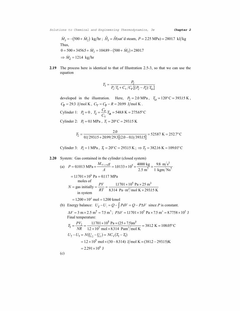
7KHSURFHVVKHUH LV LGHQWLFDO WR WKDW RI ,OOXVWUDWLRQ VR WKDWZH FDQXVH WKH
HTXDWLRQ
73
3 7 & & 3 3 7
9 3 LQ
0 5
GHYHORSHG LQ WKH LOOXVWUDWLRQ +HUH 3 03D 7LQ & . q
&3 - PRO. & & 59 3 - PRO.
&\OLQGHU 3 7&
&7 . q3
9LQ &
&\OLQGHU 3 03D 7 q & .
7
q
. &
&\OLQGHU 3 03D 7 q & . q7 . &
6\VWHP*DVFRQWDLQHGLQWKHF\OLQGHUFORVHGV\VWHP
D 30 J
$ u u
NJ
03DP
P V
NJP 1V
SLVWRQ
u 3D 03D
139
57
u u
u
u
PROHVRI
JDVLQLWLDOO\
LQV\VWHP
3D P
3D P PRO. .
PRO
NPRO
E (QHUJ\EDODQFH8 8 4 3G9 4 3 9 I ' VLQFH3LVFRQVWDQW
'9 u P P P 3 9' u u u 3D P -
)LQDOWHPSHUDWXUH
739
15
u u
u u q
3D P
PRO 3DP PRO.. &
8 8 1 8 8 1& 7 7
u u u
u
0 5 0 59
PRO - PRO. .
-
F

Solutions to Chemical and Engineering Thermodynamics, 3e Chapter 2
4 8 3 97
7
u u
u
' ''
'
RIJDV
ZRUNZRUN RI HQHUJ\ DEVRUEHG
- 0-
G 6\VWHP*DVFRQWDLQHGZLWKLQ3LVWRQ&\OLQGHURSHQV\VWHP
>1RWH6WXGHQWVWHQGWRDVVXPHG7 GW 7KLVLVWUXHEXWQRWREYLRXV@
PDVVEDODQFHG1
GW1
HQHUJ\EDODQFHG
GW18 1+
RXWQ 0
3G9
GW
+HUH 3 LV FRQVWDQW ,GHDO*DV/DZ 9 157 3 7 DQG3 RI*DV
/HDYLQJ&\OLQGHU 7 3DQG RIJDVLQWKHV\VWHP7KXV
1G8
GW8G1
GW+G1
GW3G
GW
157
3
+ 8G1
GW1&
G7
GW5G
GW17
9
57G1
GW1&
G7
GW15
G7
GW57
G1
GW1 & 5
G7
GW
G7
GW
9 9
('
0 5
4
7KXV 7 7 .
1RZJRLQJEDFNWR
1G8
GW8G1
GW+G1
GW3G9
GW DQGXVLQJ
G7
GW
G8
GW
+ 8G1
GW57
G1
GW3G9
GWRU
G1
GW
3
57
G9
GW
6LQFH3DQG7DUHFRQVWDQWV
1
1
9
9
P
P
7KXV 1 PRO u PRO
'1 PRO NPRO
D 6\VWHP*DVFRQWDLQHGZLWKLQSLVWRQF\OLQGHUFORVHGV\VWHP>QHJOHFWLQJWKH
SRWHQWLDOHQHUJ\FKDQJHRIJDV@
HQHUJ\EDODQFH
G 18
GW1G8
GW4 3
G9
GW
1&
G7
GW4 3$
GK
GW9
%XW 739
15
G7
GW
3
15
G9
GW
3$
15
GK
GW

Solutions to Chemical and Engineering Thermodynamics, 3e Chapter 2
7KXV
4$& 3
5
GK
GW$3
GK
GW3$
&
5
GK
GW
3$&
5
GK
GW
u u u u
u
9 9 3
- PRO.
- PRO.3D P P V
- V
E 6\VWHP*DVFRQWDLQHGZLWKLQSLVWRQDQGF\OLQGHURSHQV\VWHP6WDUWIURP
UHVXOWRI3DUWG3UREOHPVHHHTQ LQWKDWLOOXVWUDWLRQ
G1
GW
3
57
G9
GW
3$
57
GK
GW ZLWK3DQG7FRQVWDQW
6HHVROXWLRQWR3UREOHP
G1
GW
u u
uu
3D P
- PRO. . P V PRO V
NPRO V
0 5
>FKHFN u PRO VHF VHF PRO FRPSDUH ZLWK SDUW G RI
3UREOHP@
6\VWHPJDVFRQWDLQHGLQWKHF\OLQGHURSHQV\VWHP
,PSRUWDQWREVHUYDWLRQJDVOHDYLQJWKHV\VWHP7KDWLVHQWHULQJWKHH[LWYDOYH
RIWKHF\OLQGHUKDVVDPHSURSHUWLHVDVJDVLQWKHF\OLQGHU
PDVVEDODQFH
HQHUJ\EDODQFH
1RWHWKDWWKHVHDUH
(TQV GDQGHRI
,OOXVWUDWLRQ
G1
GW1
G 18
GW1+
()K
*K
3URFHHGLQJDVLQWKDWLOOXVWUDWLRQZHJHW(TQI
7 W
7
3 W
3
& 5
3
RU7 W
3 W5 &
3
.
0 5
ZKHUHZHKDYHXVHGDVOLJKWO\GLIIHUHQWQRWDWLRQ1RZXVLQJWKHPDVVEDODQFHZH
JHW
G1
GW
G
GW
39
57
9
5
G 3 7
GW1
0 5
RU
G 3 7
GW
15
9
0 5 0 5
u
PRO V 3D P PRO.
P3D . V
DQG

Solutions to Chemical and Engineering Thermodynamics, 3e Chapter 2
3
7
3
7W W
u
W EDU . IRU3LQEDUDQGWLQVHFV
8VLQJ W PLQXWHV VHFV LQ(TQDQGVLPXOWDQHRXVO\VROYLQJ(TQV
DQG\LHOGV
7 PLQ . 3 PLQ EDU
&RPSXWDWLRQRIUDWHVRIFKDQJHIURPPDVVEDODQFH
G
GW
3
7 7
G3
GW
3G 7
GW
15
9
OQ
RUG 3
GW
G 7
GW
157
39
OQ OQ
)URPHQHUJ\EDODQFHXVLQJHTQVDERYHDQGHTQILQ,OOXVWUDWLRQ
&
5
G 7
GW
G 3 7
GW
9 OQ OQ
0 5RU
&
5
G 7
GW
G 3
GW
3 OQ OQ
1RZXVLQJ(TQLQ(TQ7KXV
&
5
G 7
GW
&
57
G7
GW
157
39
9 9OQ
RU
G7
GW
1 57
39&WW
PLQ 9 PLQ
. VHF
DQG
G3
GW
& 3
57
G7
GW
PLQ
3
PLQ
EDU V
&RQVLGHUDIL[HGPDVVRIJDVDVWKHFORVHGV\VWHPIRUWKLVSUREOHP7KHHQHUJ\
EDODQFHLV
G 18
GW1G8
GW1&
G7
GW3G9
GW
9
)URPWKHLGHDOJDVODZZHKDYH 3 157 9 7KXV
& 1G7
GW
157
9
G9
GW
&
5
G 7
GW
G 9
GW9
9
OQ OQ
RU
&
5
7
7
9
9
7
7
9
9
& 5
9
9
OQ OQ
RU

Solutions to Chemical and Engineering Thermodynamics, 3e Chapter 2
9 7 9 7 97& 5 & 5 & 5
9 9 9 FRQVWDQW
6XEVWLWXWLQJ WKH LGHDO JDV ODZ JLYHV 39 39& &3 9 J FRQVWDQW 1RWH WKDW WKH
KHDWFDSDFLW\PXVWEHLQGHSHQGHQWRIWHPSHUDWXUHWRGRWKHLQWHJUDWLRQLQ(TQ
DVLQGLFDWHG
6\VWHP&RQWHQWVRIWKHWDQNDWDQ\WLPH
D )LQDOWHPSHUDWXUH 7 . DQGSUHVVXUH 3 u 3D2 7 DUHNQRZQ7KXVWKHUHLVQRQHHGWRXVHEDODQFHHTXDWLRQV
139
57I
3D P
- PRO.
u u
.PRO NPRO
E $VVXPHDVXVXDOWKDWHQWKDOS\RIJDVOHDYLQJWKHF\OLQGHULVWKHVDPHDVJDV
LQWKHF\OLQGHU6HH,OOXVWUDWLRQ)URP(TQIRIWKDWLOOXVWUDWLRQZH
KDYH
3
3
7
7
& 5
I
L
I
L
3
RU7
7
3
3
5 &
I
L
I
L
3
u
u
7KXV 7I . u . 3I EDU DQG
1I PRO NPRO
([FHSWIRUWKHIDFW WKDW WKHWZRF\OLQGHUVKDYHGLIIHUHQWYROXPHV WKLVSUREOHPLV
MXVWOLNH,OOXVWUDWLRQ)ROORZLQJWKDWLOOXVWUDWLRQZHREWDLQ
3
7
3
7
3
7
L
L
I
I
I
I IRU(TQD
3 3 3L I I RU 3 3I L
IRU(TQF
DQGDJDLQJHW(TQI
7
7
3
3
& 5
I
L
I
L
3
7KHQZHREWDLQ 3I EDU 7
I . DQG 7
I .
)URPSUREOHPVWDWHPHQW 3 3 3
I I I DQG 7 7 7
I I I

Solutions to Chemical and Engineering Thermodynamics, 3e Chapter 2
0DVVEDODQFHRQWKHFRPSRVLWHV\VWHPRIWZRF\OLQGHUV
1 1 1
I I L RU
3
7
3
7
3
7
3
7
I
I
I
I
I
I
L
L
(QHUJ\EDODQFHRQFRPSRVLWHV\VWHP
1 8 1 8 1 8 33
L L
I I
I I I
L
EDU
EDU
u DVEHIRUH
DQG 73
37 7 7I
I
L
L L L
.
(YHQWKRXJKWKHVHFRQGF\OLQGHULVQRWLQLWLDOO\HYDFXDWHGWKLVSUREOHPVWLOOEHDUV
PDQ\ VLPLODULWLHV WR ,OOXVWUDWLRQ 3URFHHGLQJ DV LQ WKDW LOOXVWUDWLRQ ZH
REWDLQ
3
7
3
7
3
7
3
7
L
L
L
L
I
I
I
I LQVWHDGRI(TQD
3 3 3 3 3L L I I I LQVWHDGRI(TQF
>7KXV 3I u u EDU @ DQG DJDLQ UHFRYHU (TQ I IRU
&\OLQGHU
7
7
3
3
& 5
I
L
I
L
3
(TQI
6ROXWLRQLV 3 3
EDUI I 7
I . 7
I .
D 6\VWHP *DVFRQWDLQHGLQURRPRSHQV\VWHP
PDVVEDODQFHG1
GW1
HQHUJ\EDODQFHG 18
GW1+ 4 +
G1
GW4
7KXV
4G 18
GW+G1
GW8 +
G1
GW1G8
GW
)RUWKHLGHDOJDV + 8 39 57 G1
GW
G
GW
39
57
9
5
G
GW
3
7

Solutions to Chemical and Engineering Thermodynamics, 3e Chapter 2
4 579
5
G
GW
3
71&
G7
GW57
17
3
G
GW
3
71&
G7
GW
4157
3
G3
GW15
G7
GW1&
G7
GW
9 9
9
6LQFH 3 FRQVWDQWG3
GW 4
1& G7
GW 3 RU
G7
GW
4
&
57
39
u
u u u
3
: - PRO. .
- PRO. 3D P
. V . PLQ
E 6\VWHP *DVFRQWDLQHGLQVHDOHGURRPFORVHGV\VWHP 1
(QHUJ\EDODQFHG 18
GW1G8
GW1&
G7
GW4
Y
G7
GW
4
1&
&
&
G7
GWVHDOHGURRP 9
3
9XQVHDOHGURRP
. PLQ
. PLQ
u
,QHDFKFDVHZHPXVWGRZRUNWRJHWWKHZHLJKWVRQWKHSLVWRQHLWKHUE\SXVKLQJ
WKHSLVWRQGRZQWRZKHUHLWFDQDFFHSWWKHZHLJKWVRUE\OLIWLQJWKHZHLJKWVWRWKH
ORFDWLRQRI WKH SLVWRQ :HZLOO FRQVLGHU ERWK DOWHUQDWLYHV KHUH )LUVW QRWH WKDW
FKRRVLQJWKHJDVFRQWDLQHGZLWKLQSLVWRQDQGF\OLQGHUDVWKHV\VWHP '8 4 :
%XW '8 VLQFH WKH JDV LV LGHDO DQG 7 FRQVWDQW $OVR
: 3G9 157 9 9 I OQ I L0 5 IRUWKHVDPHUHDVRQV7KXVLQHDFKFDVHZHKDYHWKDWWKHQHWKHDWDQGZRUNIORZVWRWKHJDVDUH
: 1579
9ZRUNGRQHRQJDV -I
L
u
u
OQ OQ
DQG4 : - UHPRYHGIURPJDV
,I PRUH ZRUN LV GHOLYHUHG WR WKH SLVWRQ WKH SLVWRQ ZLOO RVFLOODWH HYHQWXDOO\
GLVVLSDWLQJWKHDGGLWLRQZRUNDVKHDW7KXVPRUHKHDWZLOOEHUHPRYHGIURPWKH
JDVSLVWRQDQGF\OLQGHUWKDQLIRQO\WKHPLQLPXPZRUNQHFHVVDU\KDGEHHQXVHG
1RWHWKDWLQHDFKFDVHWKHDWPRVSKHUHZLOOSURYLGH
: 3 9DWPN3D P u u u ' -
DQGWKHFKDQJHLQSRWHQWLDOHQHUJ\RISLVWRQ
PJ K' u u u
u
NJ P V
P
P-

Solutions to Chemical and Engineering Thermodynamics, 3e Chapter 2
7KH UHPDLQGHU - PXVW EH VXSSOLHG IURP RWKHU
VRXUFHVDVDPLQLPXP
D 2QHNJZHLJKW
$QHIILFLHQWZD\RIUHWXUQLQJWKHV\VWHPWRLWVRULJLQDOVWDWHLVWRVORZO\LH
DW]HURYHORFLW\IRUFHWKHSLVWRQGRZQE\VXSSO\LQJ-RIHQHUJ\:KHQ
WKHSLVWRQLVGRZQWRLWVRULJLQDOORFDWLRQWKHNJLVVOLGVLGHZD\VRQWRWKH
SLVWRQZLWKQRHQHUJ\H[SHQGLWXUH
$Q LQHIILFLHQW SURFHVVZRXOG EH WR OLIW WKH NJZHLJKW XS WR WKH SUHVHQW
ORFDWLRQRIWKHSLVWRQDQGWKHQSXWWKHZHLJKWRQWKHSLVWRQ ,QWKLVFDVHZH
ZRXOGVXSSO\
0J K 0J9
$'
' u u
u u
u
NJ
-
P
V
P
P
NJP V
1 6
7KLVHQHUJ\ZRXOGEHWUDQVPLWWHGWRWKHJDVDVWKHSLVWRQPRYHGGRZQ7KXV
: RQJDV -DWPRVSKHUH 3( RI SLVWRQ 3( RI ZHLJKW
- -
: 4 4- - :
(IILFLHQW
,QHIILFLHQW
F\FOH F\FOH
E 7ZRNJZHLJKWV
,QWKLVFDVHZHDOVRUHFRYHUWKHSRWHQWLDOHQHUJ\RIWKHWRSPRVWZHLJKW
PJ K' u u u
NJ
P
V
P
P-
7KXVLQDQHIILFLHQWSURFHVVZHQHHGVXSSO\RQO\
-
$QHIILFLHQWSURFHVVZRXOGEHWRPRYHWKHORZHVWZHLJKWXSWRWKHSRVLWLRQRI
WKHSLVWRQE\VXSSO\LQJ
NJ
u u
u
u
P
V
P
P-
6OLGHWKLVZHLJKWRQWRWKHSLVWRQDQGOHWJR7KHWRWDOZRUNGRQHLQWKLVFDVH
LV
- DWPRVSKHUH 3( RI SLVWRQ 3( RI ZHLJKW VXSSOLHG E\ XV
' '
7KHUHIRUH

Solutions to Chemical and Engineering Thermodynamics, 3e Chapter 2
: 4 4- :
(IILFLHQW
,QHIILFLHQW -
F\FOH F\FOH
-
F )RXUNJZHLJKWV
,QWKLVFDVHWKHUHFRYHUHGSRWHQWLDOHQHUJ\RIZHLJKWVLV
NJ P V P
-
u u u
u
7KXVLQDQHIILFLHQWSURFHVVZHQHHGVXSSO\RQO\
-
$Q LQHIILFLHQWSURFHVVZRXOGEH WR UDLVH WKH ORZHVWZHLJKW XS WR WKHSLVWRQ
H[SHQGLQJ
-
NJ P V
P
P
u u u
u
7KXVWKHWRWDOZRUNGRQHLV
-
DQG
: 4 4
:
(IILFLHQW
,QHIILFLHQW
F\FOH F\FOH
G *UDLQVRIVDQG
6DPH DQDO\VLV DV DERYH H[FHSW WKDW VLQFH RQH JUDLQ RI VDQG KDV HVVHQWLDOO\
]HURZHLJKW: - 4 - : 4F\FOH F\FOH
6\VWHP *DVFRQWDLQHGLQWKHF\OLQGHUFORVHGV\VWHP
HQHUJ\EDODQFH G 18
GW1G8
GW1&
G7
GW3G9
GW
157
9
G9
GW
9 ^8VLQJ WKH
LGHDOJDVHTXDWLRQRIVWDWH`
6LQFH&9 DQG&3 DUHFRQVWDQW
&
5 7
G7
GW 9
G9
GW
9 RU
7
7
9
9
/
/
5 & 5 &
9 9
u u
q
7
P
P
. &DQG

Solutions to Chemical and Engineering Thermodynamics, 3e Chapter 2
3 39
9
7
7
EDU
u u
)URPWKHGLIIHUHQFHFKDQJHRIVWDWHIRUPRIHQHUJ\EDODQFH
'8 Q 0 I 9: 1& 7 7 3G9 0 5
DQG 139
57
u
u u
EDU
P NPRO .
. EDU PNPRO
u
: 8'
NPRO N- NPRO . .
N-
:KHUHKDVWKLVZRUNJRQH"
D 7RLQFUHDVHSRWHQWLDOHQHUJ\RISLVWRQ
E 7RLQFUHDVHNLQHWLFHQHUJ\RISLVWRQ
F 7RSXVKEDFNDWPRVSKHUHVRV\VWHPFDQH[SDQG
G :RUNGRQHDJDLQVWIULFWLRQDQGFRQYHUWHGWRKHDW
7RVHHWKLVZULWH1HZWRQ©VQG/DZRI0RWLRQIRUWKHSLVWRQ
I 0$ 3$ 3 $ PJ I PGY
GW DWP IU0 5 Y YHORFLW\RISLVWRQ
7KXV 3P
$
GY
GW3
PJ
$
I
$ DWP
IU
II I I I
'8 3G9
3 G9P
$
GY
GW
G9
GWGW
PJ
$G9
$IGY
GWGW
-
DWP IU
1RZ
$
G9
GW
GK
GWY K SLVWRQKHLJKWDQG Y
GY
GW
G
GWY
2 7
-
I3 9PY
PJ K I YGW
Y
DWP-
:RUN DJDLQVWDWPRVSKHUH
VLQFH -
:RUN XVHG WRLQFUHDVH SRWHQWLDOHQHUJ\ RI SLVWRQ
IU
LQLWLDO
' '
7KXV -
IPYI YGW
IU
D ,IWKHUHLVQRIULFWLRQ IIU WKHQ
Y Y
NJ
u
- P V P V
PJ )ULFWLRQDO )RUFH f )U
3UHVVXUH RI JDV 3 u $
f )
3DWP u $

Solutions to Chemical and Engineering Thermodynamics, 3e Chapter 2
E ,IZHDVVXPHRQO\VOLGLQJIULFWLRQ I NYIU
I YGY N Y GWPY N Y GWIUI I I
,Q RUGHU WR GHWHUPLQH WKH YHORFLW\ QRZZH QHHG WR NQRZ WKH FRHIILFLHQW RI
VOLGLQJIULFWLRQNDQGWKHQZRXOGKDYHWRVROYHWKHLQWHJUDOHTXDWLRQDERYHRU
LQWHJUDWHVXFFHVVLYHO\RYHUVPDOOWLPHVWHSV,WLVFOHDUKRZHYHUWKDW
Y YZLWKIULFWLRQ ZLWKRXWIULFWLRQ P V
q& u 3D 03D
NJ V
D PDVVEDODQFHVWHDG\VWDWH
0 0
0 0 NJ V
(QHUJ\EDODQFHQHJOHFWLQJ3(WHUPV
0 +Y
0 +Y
0 Y$ PQY$ U U PDVVGHQVLW\ Q PRODUGHQVLW\
Y YHORFLW\ $ SLSHDUHDP PROHFXODUZHLJKW
0
P
3
57Y$
Y
Y
PY
u
u u u u u
u
u u
NJ V
NJ NPRO
3D
. 3D PP V P
P V
NJ NPRO P V
NJ P 1V - NPRO N- NPRO
0 5
0 5
S
%DFNWRHQHUJ\EDODQFHQRZRQDPRODUEDVLV
+ +PY PY
& 7 7S
0 5
$VDILUVWJXHVVQHJOHFWNLQHWLFHQHUJ\WHUPV
& 7 7 7 7S & q0 51RZFKHFNWKLVDVVXPSWLRQ
YQ Y
Q
3Y
3
Y
u
u
P V
5HFDOFXODWHLQFOXGLQJWKHNLQHWLFHQHUJ\WHUPV
& 7 7PY YS - NPRO
0 5 2 7 2 7
6\VWHP IRU
SDUW D
6\VWHP IRU
SDUW E
q &
u 3D 0SD
NJV

Solutions to Chemical and Engineering Thermodynamics, 3e Chapter 2
7 7 7
u q
- NPRO
- PRO PRO NPRO&
7KXVWKHNLQHWLFHQHUJ\WHUPPDNHVVXFKDVPDOOFRQWULEXWLRQZHFDQVDIHO\
LJQRUHLW
E 0DVVEDODQFHRQFRPSUHVVRUVWHDG\VWDWH 1 1
(QHUJ\EDODQFHRQFRPSUHVVRUZKLFKLVLQVWHDG\VWDWHRSHUDWLRQ
1 + 1 + Q 0
q
: : 1 & 7 7V V S&
DGLDEDWLFFRPSUHVVRU
&DQFRPSXWH :V LI 7 LVNQRZQRUYLFHYHUVD +RZHYHUFDQQRWFRPSXWHERWK
ZLWKRXWIXUWKHULQIRUPDWLRQ
$QDO\VLVDVDERYHH[FHSWWKDW 4 z EXW :
+HUHZHJHW
%&K
'K q
1 1
4 1 & 7 7S&
&DQQRWFRPSXWH 4 XQWLO 7 LVNQRZQ
6HHVROXWLRQWR3UREOHP
D'HILQHWKHV\VWHPWREHWKHQLWURJHQJDV6LQFHD-RXOH7KRPVRQH[SDQVLRQLV
LVHQWKDOSLF + 7 3 + 7 3 0 5 0 5 8VLQJ WKH SUHVVXUH HQWKDOS\ GLDJUDP IRU
QLWURJHQ)LJXUHZHKDYH + 7 7 3 + 03D . N- NJDQGWKHQ 03D N- NJ 2 7)URPZKLFKZH ILQG WKDW7 .ZLWK DSSUR[LPDWHO\ RI WKH QLWURJHQ DV
YDSRUDQGDVOLTXLG
E $VVXPLQJ QLWURJHQ WR EH DQ LGHDO JDV SRRU DVVXPSWLRQ WKHQ WKH HQWKDOS\
GHSHQGVRQO\RQWHPSHUDWXUH6LQFHD-RXOH7KRPVRQH[SDQVLRQLVLVHQWKDOSLFWKLV
LPSOLHVWKDWWKHWHPSHUDWXUHLVXQFKDQJHGVRWKDWWKHILQDOVWDWHZLOOEHDOOYDSRU
3ODQWSURGXFHV u NZK RIHQHUJ\SHU\HDU
3ODQWXVHV u u u NZK RIKHDW
FRPSUHVVRU u 3D
7 q &
u 3D
7 "
*DV FRROHU u 3D
7 "
u 3D
7 q &

Solutions to Chemical and Engineering Thermodynamics, 3e Chapter 2
NZK - u
3ODQWXVHV u u u u- \HDU
NZKNZK - \HDU
'+ 0 & 7 7RIURFNWRWDO
NJ - J. J NJ .
-
S I L
u u u
u
0 5
u u u - \HDU \HDUV -[
[ \HDUV

6ROXWLRQV WR &KHPLFDO DQG (QJLQHHULQJ 7KHUPRG\QDPLFV H
D 6\VWHP %DOO:DWHU
(QHUJ\EDODQFH 08 0 8 08 0 8I I L L
0 & 7 7 0 & 7 7I L I L 9 9 2 7 2 7 DOVR7 7I I
7KXV
70 & 7 0 & 7
0 & 0 &
IL L
u u u u u u
u u u u
q
9 9
9 9
&
>1RWH6LQFHRQO\ '7 VDUHLQYROYHG q& ZHUHXVHGLQVWHDGRI.@
E )RUVROLGVDQGOLTXLGVZHKDYHHTQ7KDW '6 0 &G7
70&
7
7 I 3 3 OQ
IRUWKHFDVHLQ
ZKLFK&3 LVDFRQVWDQW7KXV
%DOO J-
J .
-
.
V
:DWHU J-
J .
-
.
'
'
6
6
u u
u
%&'()*
u u
u
%&'()*
OQ
OQ
DQG
'6 %DOO :DWHU-
.
-
.
1RWHWKDWWKHV\VWHP%DOO:DWHULVLVRODWHG7KHUHIRUH
'6 6 JHQ
-
.
(QHUJ\EDODQFHRQWKHFRPELQHGV\VWHPRIFDVWLQJDQGWKHRLOEDWK
0 & 7 7 0 & 7 7F FI
FL
R RI
RL
9 9 2 7 2 7 VLQFHWKHUHLVDFRPPRQILQDOWHPSHUDWXUH
NJ NJ u
u
N-
NJ ..
N-
NJ ..7 7I I3 8 3 8
7KLVKDVWKHVROXWLRQ7I R& .
6LQFH WKH ILQDO WHPSHUDWXUH LV NQRZQ WKH FKDQJH LQ HQWURS\ RI WKLV V\VWHP FDQ EH FDOFXODWHG
IURP '6 u u
u u
OQ
OQ
N-
.
&ORVHGV\VWHPHQHUJ\DQGHQWURS\EDODQFHV
G8
GW4 : 3
G9
GWV
G6
GW
4
76
JHQ
7KXVLQJHQHUDO 4 7G6
GW76
JHQDQG

6ROXWLRQV WR &KHPLFDO DQG (QJLQHHULQJ 7KHUPRG\QDPLFV H
:G8
GW4 3
G9
GW
G8
GW7G6
GW76 3
G9
GWV JHQ
5HYHUVLEOHZRUN : : 6G8
GW7G6
GW3G9
GWV V
5HY 5HYJHQ 2 7
D 6\VWHPDWFRQVWDQW89 G8
GW DQG
G9
GW
W S W TdS
dts gen S 02 7 Rev
E 6\VWHPDWFRQVWDQW63 G6
GW DQG
G3
GW3G9
GW
G
GW39
VRWKDW
: 6 :G8
GW
G
GW39
G
GW8 39
G+
GWV JHQ 6 2 7 UHY
EDUR&EDU7 "
6WHDG\VWDWHEDODQFHHTXDWLRQV
G0
GW0 0
G8
GW0 + 0 + Q 0
Ws
03
dV
dt
0 0 + 0 +
RU + +
'UDZLQJDOLQHRIFRQVWDQWHQWKDOS\RQ0ROOLHU'LDJUDPZHILQGDW 3 EDU 7 # q &
$WEDUDQG & $WEDUDQG &
P NJ P NJ
N- NJ N- NJ
N- NJ. N- NJ.
q q
|
|
9 9
+ +
6 6
$OVR
G6
GW0 6 0 6
0Q
T JHQ
6
6 0 6 6JHQ 2 7 RU
6
06 6
JHQ N-
NJ .
6\VWHP
(QHUJ\EDODQFH
'8 8 8 8 8I L I L 2 7 2 7 Q adiabat i :6 PdVI
constan
volume
:V

6ROXWLRQV WR &KHPLFDO DQG (QJLQHHULQJ 7KHUPRG\QDPLFV H
: 0& 7 7 0& 7 7 0& 7 7 7 7V
I L I L I L I L S S S 2 7 2 7 2 7 2 7
EXW 7 7 7:
0&7 7 7I I I V I L L
3
(QWURS\EDODQFH
'6 6 6 6 6I L I L 2 7 2 7
Q
TdtI
0adiabatic
Sgen
0 for maximum wo r
6 6 6 6 0&7
70&
7
7
I L I LI
L
I
L
2 7 2 7 3 3OQ OQ
RU OQ7 7
7 7
I I
L L
%&'
()* 7 7 7 7I I L L
EXW 7 7 7I I I
7 7 7I L L2 7 2 7
RU 7 7 7I L L
DQG
:
0&7 7 7 7 7 7 7V I L L L L L L
3
D (QWURS\FKDQJHSHUPROHRIJDV
'6 &7
75
3
3
3OQ OQ
HTQ
7KXV '6
OQ OQ
-
PRO.
-
PRO.
-
PRO.
E 6\VWHP FRQWHQWVRIWXUELQHVWHDG\VWDWHV\VWHP
0DVVEDODQFHG1
GW1 1 1 1 1
(QHUJ\EDODQFHG8
GW1 + 1 + Q 0
V: 3
dV
dt
0
: 1 + + 1& 7 7V 0 5 0 53
::
1& 7 7V u
3
-
PRO..
-
PRO
0 5
F ,Q ,OOXVWUDWLRQ : - PRO EHFDXVH RI LUUHYHUVLEOLWLWLHV '6 z PRUH ZRUN LV
GRQHRQWKHJDVKHUH:KDWKDSSHQVWRWKLVDGGLWLRQDOHQHUJ\LQSXW",WDSSHDUVDVDQLQFUHDVHRI
WKHLQWHUQDOHQHUJ\WHPSHUDWXUHRIWKHJDV
+HDWORVVIURPPHWDOEORFN
G8
GW&
G7
GW4
3
EDU
.
EDU
.

6ROXWLRQV WR &KHPLFDO DQG (QJLQHHULQJ 7KHUPRG\QDPLFV H
%&'
:
7 7
74
4
4
KHDWRXWRIPHWDO
KHDWLQWRKHDWHQJLQH
&G7
GW
7 7
7: :GW &
7
7G7
: & 7 7 & 77
7& 7 7 7
7
7
: & 77
7
7
7
4 & G7 & 7 7 & 77
7
W
7
7
7
7
3 3
3 3 3
3
3 3 3
!
"$#
!
"$#
I I
I
0 5
0 5 0 5
0 5
OQ OQ
OQ
$OWHUQDWHZD\WRVROYHWKHSUREOHP
6\VWHPLVWKHPHWDOEORFNKHDWHQJLQHFORVHG
(%G8
GW&
G7
GW4 : 3
6%G6
GW
4
7
Sgen
0 for maximum wo r
4 7G6
GW
G8
GW7
G6
GW: G8 & G7 3 G6
&
7G7 3
:G8
GW7
G6
GW& G7 7
&
7G7 &
7
7G7
33
3
: :GW &7
7G7 &
7
7G7
: & 7 7 7 &7
7& 7
7
7
7
7
7
7
7
7
!
"$#
I I I
OQ OQ
3 3
3 3 3
0 5
7KLVSUREOHPLVQRWZHOOSRVHGVLQFHZHGRQRWNQRZH[DFWO\ZKDWLVKDSSHQLQJ7KHUHDUHVHYHUDO
SRVVLELOLWLHV
:DWHUFRQWDFW LVYHU\VKRUW VRQHLWKHUVWUHDPFKDQJHV7YHU\PXFK ,Q WKLVFDVHZHKDYH WKH
&DUQRWHIILFLHQF\
K
:
4
7 7
7
KLJK ORZ
KLJK
%RWKZDUPVXUIDFHZDWHUq&DQGFROGGHHSZDWHUq&HQWHUZRUNSURGXFLQJGHYLFHDQG
WKH\OHDYHDWDFRPPRQWHPSHUDWXUH
7
7+
7/
72

6ROXWLRQV WR &KHPLFDO DQG (QJLQHHULQJ 7KHUPRG\QDPLFV H
0%G0
GW0 0 0 0 0 0
+ / + /1 6
(%G8
GW0 + 0 + 0 + :
+ + / /
: 0 + 0 + 0 0 +
0 + + 0 + +
0 & 7 7 0 & 7 7
+ + / / + /
+ + / /
+ 3 + / 3 /
1 6
2 7 2 70 5 0 5
6%G6
GW0 6 0 6 0 6
+ + / /
Q
T
0Sgen
0
OQ OQ
0 6 0 6 0 0 6
0 6 6 0 6 6 0 &7
70 &
7
7
7
7
7
77 7 7
0 0
0 0 0 0
+ + / / + /
+ + / / + 3
+
/ 3
/
+ /
+ /
+ /
+ / + /RU
1 6
2 7 2 7
7 7 70 0 0 0 0 0
+ /
+ + / / + / 1 6 1 6
)URPWKLVFDQFDOFXODWH 77KHQ
: 0 & 7 7 0 & 7 7 + 3 + / 3 / 0 5 0 5
7KLVFDQEHXVHGIRUDQ\IORZUDWHUDWLR
6XSSRVHYHU\ODUJHDPRXQWRIVXUIDFHZDWHULVFRQWDFWHGZLWKDVPDOODPRXQWRIGHHSZDWHULH 0 0+ /!! 7KHQ 7 7
a
+
a : 0 & 7 7 0 & 7 7 0 & 7 7 + 3 + + / 3 + / / 3 + /0 5 0 5 0 5
6XSSRVHYHU\ODUJHDPRXQWRIGHHSZDWHULVFRQWDFWHGZLWKDVPDOODPRXQWRIVXUIDFHZDWHULH 0 0+ / 7 7
a
/
a : 0 & 7 7 0 & 7 7 0 & 7 7 + 3 / + / 3 / / + 3 / +0 5 0 5 0 5
6\VWHP FRQWHQWVRIWKHWXUELQH7KLVLVDVWHDG\VWDWHDGLDEDWLFFRQVWDQWYROXPHV\VWHP
D 0DVVEDODQFHG0
GW0 0
RU 0 0
(QHUJ\EDODQFH
G8
GW0 + 0 +
Q adiabat i
: 3V
dV
dt
constan
volume
(QWURS\EDODQFH
G6
GW0 6 0 6
Q
TSgen
0, by problem state m
7KXV 0 0
NJ K 0%
: 0 + +6
2 7 (%
6 6 6%

6ROXWLRQV WR &KHPLFDO DQG (QJLQHHULQJ 7KHUPRG\QDPLFV H
6WDWH
7
q&
3
EDU 7DEOHV
6WHDP o
+
N- NJ
6
N- NJ
6WDWH
3 EDU
6 6 N-
NJ.
7DEOHV
6WHDP o
7 # q &
+ | N- NJ
:V u
NJ
K
N-
NJ
N-
KN:
E 6DPHH[LWSUHVVXUH 3 EDU 0 5 DQGVWLOODGLDEDWLF : 0 + +
V 2 7 +HUHKRZHYHU
: : +V V u
3DUWDN-
K
N-
K2 7 2 7
+
3
EDU
N- NJ
7DEOHV
6WHDP o
7
6
#
|
.
N- NJ.
7KXV
6 0 6 6JHQ
NJ
K
N-
NJ.
N-
. K u
2 7
F )ORZDFURVVYDOYHLVD-RXOH7KRPSVRQLVHQWKDOSLFH[SDQVLRQ6HH,OOXVWUDWLRQ
7KXV + +LQWR YDOYH RXW RI YDOYH DQGWKHLQOHWFRQGLWLRQVWRWKHWXUELQHDUH
+ + +
3
EDU
RXW RI YDOYH LQWR YDOYH N- NJ
7DEOHV
6WHDP o
7
6
| q
|
&
N- NJ.
)ORZDFURVVWXUELQHLVLVHQWURSLFDVLQSDUWD
6 6
3
EDU
N- NJ.
7DEOHV
6WHDP o
7
+
# q
|
&
N- NJ
:V u u N:NJ
K
N-
NJ
N-
K
6LQFHFRPSUHVVLRQLVLVHQWURSLFDQGJDVLVLGHDOZLWKFRQVWDQWKHDWFDSDFLW\ZHKDYH
7
7
3
3
5 &
3
6RWKDW7 73
3
5 &
u
u
3
.
1RZXVLQJIURPVROXWLRQWR
3UREOHPWKDW : 1& 7 7V 3 0 5

6ROXWLRQV WR &KHPLFDO DQG (QJLQHHULQJ 7KHUPRG\QDPLFV H
:V u u u u
u
J
NJ
V
PRO
J
-
PRO..
NJ
- V
7KHORDGRQWKHJDVFRROHULVIURP3UREOHP
4 1& 7 7
.
u
u u
u
S
NJ V J NJ
J PRO
-
PRO.
- V
0 5

3.11 (a) This is a Joule-Thomson expansion ⇒ =( ) = = °( ) ≈ = °( )=
$ ? $ . $
.
H T H T H T70 bar, 10133 400 1 400
32782
bar, C bar, C
kJ kg
and T = °447 C , $ .S = 6619 kJ kg K
(b) If turbine is adiabatic and reversible &Sgen = 0c h , then $ $ .S Sout in kJ kg K= = 6619 and P = 1013.
bar. This suggests that a two-phase mixture is leaving the turbine
Let fraction vapor kJ kg K
kJ kg K
V
Lx
S
S=
=
=
$ .$ .
7 3594
13026
Then x x7 3594 1 13026 6619. . .( ) + −( )( ) = kJ kg K or x = 08778. . Therefore the enthalpy offluid leaving turbine is
$ . . . . .$ $
HH H
= × + −( ) × =( ) ( )
08788 26755 1 08778 417 46 2399 6V L sat’d, 1 bar sat’d, 1 bar
kJ
kg
Energy balance
0 = + +& $ & $M H M Hin in out out&Q0 + −&W Ps
dV
dt
0
but & &M Min out= −
⇒ − = − =&
& . . .W
Ms
in
kJ
kg3278 2 2399 6 8786
(c) Saturated vapor at 1 bar
$ . ; $ .
& . . .
%.
..
&
& . . .
S H
W
M
S
M
s
= =
− = − =
( ) = × =
= − =
7 3594 26755
32782 26755 602 7
602 7 100
8786686%
7 3594 6619 0740
kJ kg K kJ kg
kJ kg
Efficiency
kJ Kh
in Actual
gen
in
(d) 0
0
0
1 2 2 1
1 1 2
1 1 2
= + ⇒ = −
= − + + −
= − + +
& & & &
& $ $ & &
& $ $&
&
M M M M
M H H W Q PdV
dt
M S SQ
TS
sc h
c h gen
Simplifications to balance equations
&Sgen = 0 (for maximum work); PdV
dt= 0 (constant volume)
& &Q
T
Q
T=
0
where T0 25= °C (all heat transfer at ambient temperature)
W
Q
Water1 bar25° C
Steam70 bar447° C

$ .H sat'd liq, 25 CkJ
kg°( ) = 10489 ; $ .S T sat'd liq, 25 C
kJ
kg K= °( ) = 03674
&
&$ $Q
MT S S= −0 2 1c h ;
− = − + − = − − −&
&$ $ $ $ $ $ $ $
max
W
MH H T S S H T S H T Ss
1 2 0 2 1 1 0 1 2 0 2c h c h c h
− = − × − − ×
= + =
&
& . . . . . .
. . .max
W
Ms 32782 29815 6619 10489 29815 03674
1304 75 4 65 1309 4 kJ kg
3.12 Take that portion of the methane initially in the tank that is also in the tank finally to be in thesystem. This system is isentropic S Sf i= .
(a) The ideal gas solution
S S T TP
P
NPV
RTN
PV
RTN
P V
RT
N N N
f i f if
i
R C
ii
if
f
f
f i
p
= ⇒ = FHG
IKJ = F
HIK =
⇒ = = = =
= − = −
30035
701502
1964 6 mol; 1962
17684
8 314 36..
. .
.
.
K
= mol
mol∆
(b) Using Figure 2.4-2.
70 bar ≈ 7 MPa, T = 300 K $ . $S Si f= =505 kJ kg K
$ . ,.
.
.V m
N
i i
i
= = =
=×
=
0019507
00195
3590 kg.
35.90 kg1282
m
kg so that
m
mkg
1000gkg
28g
mol
mol
3 3
3
At 3.5 bar = 0.35 MPa and $ .S Tf = ⇒ ≈505 138 K. kJ kg K Also,
$ . ,.
.
.
..
V m
N
f f
f
= = =
=×
=
019207
0192
3646 kg.
3646 kg1302
m
kg so that
m
mkg
1000gkg
28g
mol
mol
3 3
3
∆N N Nf i= − = − = −1302 1282 11518 mol. .
3.13 dS CdT
TR
dV
V= + eqn. (3.4-1)
∆S a R bT cT dTe
T
dT
TR
dV
V= −( ) + + + +L
NMOQP + zz 2 3
2
so that

S T V S T V a RT
Tb T T
cT T
dT T
eT T R
V
V
2 2 1 12
12 1 2
212
23
13
22
12 2
1
2
3 2
, , ln
ln
a f a f a f c h
c h c h
− = −( ) + − + −
+ − − − +− −
Now using
PV RTV
V
T
T
P
P
S T P S T P aT
Tb T T
cT T
dT T
eT T R
P
P
= ⇒ = ⋅ ⇒
− = + − + −
+ − − − −− −
2
1
2
1
1
2
2 2 1 12
12 1 2
212
23
13
22
12 2
1
2
3 2
, , ln
ln
a f a f a f c h
c h c h
Finally, eliminating T2 using T T P V PV2 1 2 2 1 1= yields
S P V S P V aP V
PV
b
RP V PV
c
RP V PV
d
RP V PV
eRP V PV R
P
P
2 2 1 12 2
1 12 2 1 1
2 2 22
1 12
3 2 23
1 13
2
2 22
1 12 2
1
2
3
2
, , ln
ln
a f a f a f
a f a f
a f a f
d i d i
− =FHG
IKJ + −
+ −
+ −
− − −− −
3.14 System: contents of valve (steady-state, adiabatic, constant volume system)
Mass balance 0 1 2= +& &N N
Energy balance 0 1 1 2 2= + +& &N H N H &Q 0 +Ws
0−P
dV
dt
0
⇒ =H H1 2
Entropy balance0 1 1 2 2= + + +& & &N S N S Sgen
&Q
T
0
⇒ = − =∆S S SS
N2 1
&
&gen
(a) Using the Mollier Diagram for steam (Fig. 2.4-1a) or the Steam Tables
T
P
P
H
T
S1
1
2
2
2
2
600 K
35
7
30453
293
7 277
==
==
⇒≈ °= bar
bar
J g
C
J g K$ . $ .
$ $ .H H1 2 30453= = J g . Thus $ .S1 65598 = J g K ; Texit C= °293
∆ $ $ $ .S S S= − =2 1 0717 J g K
(b) For the ideal gas, H H T T1 2 1 2 600 K= ⇒ = =

∆
∆
S S T P S T P CT
TR
P
P
RP
P
S
= − = −
= − = ⇒
=
2 2 1 12
1
2
1
2
1
1338
0743
, , ln ln
ln .
$ .
a f a f p
J mol K
J mol K
3.15 From the Steam Tables
At 200oC,
P
V V
U U
H H
S S
H S
L V
L V
L L
L V
=
= =
= =
= =
= ⋅ = ⋅
= = ⋅
15538 MPa
0001157 012736 m
85065 25953
852 45 27932
2 3309 64323
19407 41014
.$ . / $ . /
$ . / $ . /$ . / $ . /
$ . / $ . /
$ . $ .
m kg kg
kJ kg kJ kg
kJ kg kJ kg
kJ kg K kJ kg K
kJ / kg kJ / kg K
3 3
vap vap∆ ∆(a) Now assuming that there will be a vapor-liquid mixture in the tank at the end, the properties
of the steam and water will be
At 150oC,
P
V V
U U
H H
S S
H S
L V
L V
L V
L V
=
= =
= =
= =
= ⋅ = ⋅
= = ⋅
04578 MPa
0001091 03928 m
63168 kJ 25595
632 20 kJ 27465
18418 kJ 68379
2114 3 4 9960 kJ
.$ . / $ . /
$ . / $ . /$ . / $ . /
$ . / $ . /
$ . / $ . /
m kg kg
kg kJ kg
kg kJ kg
kg K kJ kg K
kJ kg kg K
3 3
vap vap∆ ∆
(b) For simplicity of calculations, assume 1 m3 volume of tank.Then
Mass steam initially = 0.8 m
0.12736 m kg kg
Mass water initially = 0.2 m
0.001157 m kg
Weight fraction of steam initially =6.2814
179.14
Weight fraction of water initially =6.2814
179.14
3
3
3
3
/.
/.
.
.
=
=
=
=
62814
17286 kg
003506
096494
The mass, energy and entropy balances on the liquid in the tank (open system) at any timeyields
dM
dtM
dM U
dtM H
dM S
dtM S
MdU
dtU
dM
dtM H H
dM
dt
MdU
dt
dM
dtH U
LL
L LL V
L LL V
LL
LL
L V VL
LL L
V L
= = =
+ = =
= −
& ;$
& $$
& $
$$ & $ $
$$ $
; and
or
c hAlso, in a similar fashion, from the entropy balance be obtain
MdS
dt
dM
dtS S
dM
dtSL
L LV L
L$$ $ $= − =c h ∆ vap

There are now several ways to proceed. The most correct is to use the steam tables, and to useeither the energy balance or the entropy balance and do the integrals numerically (since theinternal energy, enthalpy, entropy, and the changes on vaporization depend on temperature.This is the method we will use first. Then a simpler method will be considered.Using the energy balance, we have
dM
M
dU
H U
M M
M
U U
H UM M
U U
H U
L
L
L
V L
iL
iL
iL
iL
iL
iV
iL i
LiL i
LiL
iV
iL
=−
− = −−
= + −−
FHG
IKJ
+ ++
+
$
$ $ ,
$ $
$ $
$ $
$ $
or replacing the derivatives by finite differences
or finally 1 11
11
So we can start with the known initial mass of water, then using the Steam Tables and the dataat every 5oC do a finite difference calculation to obtain the results below.
i T (oC) $UiL (kJ/kg K) $Hi
V (kJ/kg K) MiL (kg)
1 200 850.65 2793.2 172.862 195 828.37 2790.0 170.883 190 806.19 2786.4 168.954 185 784.10 2782.4 167.065 180 762.09 2778.2 165.226 175 740.17 2773.6 163.427 170 718.33 2768.7 161.678 165 696.56 2763.5 159.959 160 674.87 2758.1 158.2710 155 653.24 2752.4 156.6311 150 631.68 2746.5 155.02
So the final total mass of water is 155.02 kg; using the specific volume of liquid water at150oC listed at the beginning of the problem, we have that the water occupies 0.1691 m3
leaving 0.8309 m3 for the steam. Using its specific volume, the final mass of steam is found tobe 2.12 kg. Using these results, we find that the final volume fraction of steam is 83.09%, thefinal volume fraction of water is 16.91%, and the fraction of the initial steam + water that hasbeen withdrawn is(172.86+6.28-155.02-2.12)/(172.86+6.28) = 0.1228 or 12.28%. A total of 22.00 kg of steamhas withdrawn, and 87.7% of the original mass of steam and water remain in the tank.
For comparison, using the entropy balance, we have
dM
M
dS
S S
M M
M
S S
SM M
S S
S
L
L
L
V L
iL
iL
iL
iL
iL
iiL
iL i
LiL
i
=−
− = − = + −FHG
IKJ
+ ++
+
$
$ $ ,
$ $
$
$ $
$
or replacing the derivatives by finite differences
of finally vap vap
1 11
11∆ ∆
So again we can start with the known initial mass of water, then using the Steam Tables andthe data at every 5oC do a finite difference calculation to obtain the results below.
i T (oC) $SiL (kJ/kg K) $Si
L (kJ/kg K) MiL (kg)
1 200 2.3309 6.4323 172.862 195 2.2835 6.4698 170.863 190 2.2359 6.5079 168.924 185 2.1879 6.5465 167.025 180 2.1396 6.5857 165.176 175 2.0909 6.6256 163.367 170 2.0419 6.6663 161.608 165 1.9925 6.7078 159.879 160 1.9427 6.7502 158.18

10 155 1.8925 6.7935 156.5311 150 1.8418 6.8379 154.91
So the final total mass of water is 154.91 kg; using the specific volume of liquid water at150oC listed at the beginning of the problem, we have that the water occupies 0.1690 m3
leaving 0.8310 m3 for the steam. Using its specific volume, the final mass of steam is found tobe 2.12 kg. Using these results, we find that the final volume fraction of steam is 83.10%, thefinal volume fraction of water is 16.90%, and the fraction of the initial steam + water that hasbeen withdrawn is(172.86+6.28-154.91-2.12)/(172.86+6.28) = 0.1234 or 12.34%. A total of 22.11 kg of steamhas withdrawn, and 87.7% of the original mass of steam and water remain in the tank.
These results are similar to that from the energy balance. The differences are the result ofround off errors in the simple finite difference calculation scheme used here (i.e., morecomplicated predictor-corrector methods would yield more accurate results.).
A simpler method of doing the calculation, avoiding numerical integration, is to assume thatthe heat capacity and change on vaporization of liquid water are independent of temperature.Since liquid water is a condensed phase and the pressure change is small, we can make thefollowing assumptions$ $ $ $ $
$ $;
$
U H H H H
dU
dt
dH
dtC
dT
dt
dS
dt
C
T
dT
dt
L L V L
L LL
L L L L
≈ − =
≈ ≈ ≈
and
and
vap
PP
∆
With these substitutions and approximations, we obtain from the energy balance
MdU
dt
dM
dtH U M
dH
dt
dM
dtH
M CdT
dt
dM
dtH
C H
C
H
dT
dt M
dM
dt
C
H
M
M
LL L
V L LL L
L LL
L
L
L
L
LfL
iL
$$ $
$$
$
$
$
$ ln
= − → =
=
=
−( ) =FHG
IKJ
c h
Now using an average value of and over the temperature range we obtain
or
vap
Pvap
Pvap
Pvap
Pvap
∆
∆
∆
∆
∆
1
150 200
and from the entropy balance
MdS
dt
dM
dtS M
C
T
dT
dt
dM
dtS
C S
C
T S
dT
dt M
dM
dt
C
S
M
M
LL L
LL L
L
L
L
L
LfL
iL
$$ $
$
$
$ln
.
.ln
= → =
=
++
FH
IK =
FHG
IKJ
∆ ∆
∆
∆
∆
vap P vap
Pvap
Pvap
Pvap
Now using an average value of and over the temperature range we obtain
or1
150 27315
200 27315
From the Steam Table data listed above, we obtain the following estimates:

CU T U T
CT
TS T S T
CS T S T
L
L
L
P
o o
o o
P
P
o o
C C
C - C
kJ
kg K
or using the ln mean value (more appropriate for the entropy calculation) based on
C C kJ
kg K
= = − = = − =⋅
FHG
IKJ = −
= = − =++
FH
IK
= −FH
IK
=⋅
$ ( ) $ ( ) . ..
ln $ $
$( ) $( )
ln..
. .
ln..
.
200 150
200 150
852 45 632 20
504 405
200 150200 27315150 27315
2 3309 184184731542315
4 3793
2
12 1a f a f
Also, obtaining average values of the property changes on vaporization, yields
∆ ∆ ∆
∆ ∆ ∆
$ $ $ . . .
$ $ $ . . .
H H T H T
S S T S T
vap vap o vap o
vap vap o vap o
C CkJ
kg
C CkJ
kg K
= × = + = = × + =
= × = + = = × + =⋅
1
2150 200
1
22114 3 19407 20275
1
2150 200
1
24 9960 41014 45487
b g b g
b g b gWith this information, we can now use either the energy of the entropy balance to solve theproblem. To compare the results, we will use both (with the linear average Cp in the energybalance and the log mean in the entropy balance. First using the energy balance
C
H
M
M
M
M
LfL
iL
fL
iL
Pvap∆ $ ln
.
..
exp . .
150 2004 405 50
20275010863
010863 089706
−( ) =FHG
IKJ = − × = −
= −( ) =
Now using the entropy balance
ln $ ln.
.
.
.ln
.
.. ln
.
.
.
..
.
M
M
C
S
M
M
fL
iL
L
fL
iL
FHG
IKJ = +
+FH
IK = F
HIK = F
HIK
= FH
IK =
Pvap∆
150 27315
200 27315
4 3793
45487
42315
4731509628
42315
47315
42315
47315089805
0 9628
Given the approximations, the two results are in quite good agreement. For what follows, theenergy balance result will be used. Therefore, the mass of water finally present (per m3) is
M M
V M V
MV
L L
L L o 3
3
V3
V o
3
3
final initial
occupying final C m
Therefore, the steam occupies 0.8308 m , corresponding to
final0.8308 m
C
0.8308 mmkg
kg
( ) = × ( ) =
= ( ) × = × =
( ) = = =
0897 15506 kg
150 15506 0001091 01692
150 039282115
. .$ . . .
$.
.
b g
b g
So the fraction of liquid in the tank by mass at the end is 155.06/(155.06+2.12) = 0.9865,though the fraction by volume is 0.1692. Similarly the fraction of the tank volume that issteam is 0.8308, though steam is only 2.12/(155.06+2.12) = 0.0135 of the mass in the tank.
(c) Initially there was 6.28 + 172.86 = 179.14 kg of combined steam and water, and finally fromthe simpler calculation above there is 155.06 + 2.12 = 157.18 kg. Therefore, 87.7% of thetotal amount of steam + water initially in the tank are there finally, or 12.3% has beenwithdrawn. This corresponds to 21.96 kg being withdrawn. This is in excellent agreementwith the more rigorous finite difference calculations done above.

3.16 (a)dN
dtN N N N= = + = −0 1 2 2 1& & ; & & or
dU
dtN H N H W Q P
dV
dtW N H N H
W
NH HS S
S= = + + + − = + −0 1 1 2 2 1 1 1 21
2 1& & & & & & &
&
& or = -
dS
dtN S N S
Q
TS
S
NS S= = − + + = −0 1 1 1 2
0 12 1
& &&
&&
&gengen CP
J
mol K=
⋅37151.
= - = KP298.15K
P
&
& .W
NH H C dT C TS
T
f
f
12 1 29815z = ⋅ −c h if the heat capacity is independent of
temperature. First consider the reversible case,
S SC
TdT R
dP
PT
T
i
f
2 11
10
0 gives − = = zz P The solution is 499.14K. Then
KJ
molP
&
& . .W
NCS
rev
1
49914 29815 7467= ⋅ −( ) = . The actual work is 25% greater
W W C T
T
act Srev
f
f
= = = ⋅ −
=
125 9334 29815
549 39
. .
.
J
molK
The solultion is K
P c h
(b) Repeat the calculation with a temperature-dependent heat capacity
C T T T TP( ) = + ⋅ − ⋅ + ⋅− − −22 243 5977 10 3499 10 7 464 102 5 2 9 3. . . .Assuming reversibility Tf = 479.44K. Repeating the calculations above with the temperature-dependent heat capacity we find Wact = 9191 J, and Tf =520.92K.So there is a significant difference between the results for the constant heat capacity and variableheat capacity cases.
3.17 T T Pi f i = 300 K, = 800 K, and = 1.0 bar
C T T T TP-2 -5 2 -9 3( ) = 29.088 - 0.192 10 + 0.4 10 - 0.870 10
J
mol K× × ×
⋅
C T
TdT P
dP
P
P
W C T dT
T
T
P
P
f
revT
T
i
f
i
f
i
f
P
K
K
6
PK
K
Calculated final pressure = 3.092 10 Pa.
J
mol
( )
( ) .
=
=
=
=
=
z z
z
=
×
= = ×
300
800
1
300
80041458 10
3.18 Stage 1 is as in the previous problem.Stage 2Following the same calculation as above.
Stage 2 allowed pressure = 9.563 10 Pa
= 1.458 10 J
mol = Stage 2 work
,7
rev-4
P
W
f 2 ×
×

Stage 3
Following the same calculation method
= 2.957 10 Pa = Stage 3 allowed pressure.
= 1.458 10J
mol = Stage 3 work
,-9
rev4
P
W
f 3 ×
×
Question for the student: Why is the calculated work the same for each stage?
3.19 The mass, energy and entropy balances aredM
dtM M M M
dU
dtM H M H Q W M H H W
W M H H
dS
dtM S M S
Q
TS M S S S
S M S S
= + = = −
= = + + + − + =
= + −
= = + + + = − + =
= −
& & , & &
& $ & $ & & ; & $ $ & ;
& & $ $
& $ & $&
& & $ $ &
& & $ $
1 2 2 1
1 1 2 2 1 1 2
1 2 1
1 1 2 2 1 1 2
1 2 1
0
0 0
0 0
s s
s
gen gen
gen
c hc h
c hc h
300 05° =C, 5 bar MPa. $ .H1 3064 2= kJ kg$ .S1 7 4599= kJ kg K
100 01° =C, 1 bar MPa. $ .H2 26762= kJ kg$ .S2 7 3614= kJ kg K
&
& . .W
Ms kJ kg1
2676 2 3064 2 388 = − = satisfied the energy balance.
&
&$ $ . . .
S
MS Sgen kJ kg K
12 1 7 3614 7 4599 00985= − = − = − can not be. Therefore the process is impossible.
3.20 Steam 20 bar 2= ° MPa and 300 C $ .H = 30235 kJ kg$ .S = 67664 kJ kg (from Steam Tables)$ .U = 2772 6 kJ kg
Final pressure = 1 bar. For reference saturation conditions areP T= =01 99 63. . MPa, $ .U L = 417 36 $ .HL = 417 46 $ .SL = 13026$ .U V = 25061 $ .HV = 26755 $ .SV = 7 3594
(a) Adiabatic expansion valve & &W Q= =0 and 0
M.B.:dM
dtM M= + =& &
1 2 0 ; & &M M2 1= − ;
E.B.:dU
dtM H M H= + =& $ & $
1 1 2 2 0 ; $ $H H2 1=
From Steam Tables⇒ H2 30235= . T = °250 C $ .H = 29743 kJ kg $ .S = 80333 kJ kg K
P = 01. MPa T = °300 C $ .H = 3074 3 kJ/kg $ .S = 82158 kJ/kg K
By interpolation T H= ° ⇒275 C gives = 3023.5 kJ / kg$ all vapor

$ .
& $ & $ &
&
&$ $ .
S
dS
dtMS M S S
S
MS S
=
= + + =
= − − =
81245
0
1359
1 2 2
2 1
kJ kg K
= 8.1254 6.7664 kJ kg K
gen
gen
gen
(b) Well designed, adiabatic turbine
E.B.: & $ & $ &M H M H W1 1 2 2 0+ + = ; & $ $W H H= −2 1c hS.B.: & $ & $M S M S1 1 2 2 0+ = ; $ $S S2 1= ; $ .S2 67664= kJ kg K
⇒ Two-phase mixture. Solve for fraction of liquid using entropy balance.
x x
x
⋅ ( ) + −( ) ⋅ == ( )7 3594 1 13026 6 7664
0 902
. . .
. not good for turbine!$ . . . . .&
& . . .
&
& .
H
W
M
W
M
2 0902 26755 0098 417 46 2454 2
2454 2 30235 569 3
569 3
= × + × =
= −( ) = −
− =
kJ kg
kJ kg
kJ kg
(c) Isorthermal turbine ⇒ superheated vapor
T
P
= °=
OQP
300
01
C
MPa final state
.
$ .
$ .
H
S
=
=
3074 3
82158
kJ kg
kJ kg K
E.B.: & $ & $ & &M H M H Q W1 1 2 2 0+ + + =s
S.B.: & $ & $&
M S M SQ
T1 1 2 2+ + +Sgen0
= 0
&& $ & $ & $ $
&
&$ $ . . .
.&
&
&
&$ $ . . . .
Q
TM S M S M S S
Q
MT S S
W
M
Q
MH H
= − − = −
= − = +( ) −( )
=
− = + − = + −( ) =
1 1 2 2 1 2 1
2 1
1 2
300 27315 82158 67664
8307
8307 30235 3074 3 779 9
c h
c h
c h
kJ kg K
kJ kg
kJ kgs
⇒ get more work out than in adiabatic case, but have to put in heat.

6\VWHP FRQWHQWVRIWKHFRPSUHVVRUVWHDG\VWDWHFRQVWDQWYROXPH$OVRJDVLVLGHDO
D 0DVVEDODQFH
o 1 1 1 1
(QHUJ\EDODQFH
1 + 1 + Q 0
adiabatic
: 3V
dV
dt
0
(QWURS\EDODQFH
1 6 1 6Q
T
0Sgen
0
reversib l
compresso r
6 6
)URPWKHHQHUJ\EDODQFH : 1& 7 7V
3 0 5 RU
:
1& 7 7V 3 0 5
)URPWKHHQWURS\EDODQFH 6 6 7 73
3
5 &
3
7KXV
:
1& 7
3
3
V
5 &
!
"
$##
3
3
E 7ZRVWDJHFRPSUHVVLRQZLWKLQWHUFRROLQJVRWKDWJDVLVUHWXUQHGWRLQLWLDO WHPSHUDWXUHEHIRUH
HQWHULQJQGFRPSUHVVRU
ZRUNLQVWDJH
!
"
$##
: 1& 73
3V
,
5 &
3
3
ZKHUH 3 SUHVVXUHDIWHUVWFRPSUHVVRU
ZRUNLQVWDJH
!
"
$#
: 1& 73
3V
,,
5 &
3
3
7RWDOZRUN
!
"
$##
: : 1& 73
3
3
3:
V
,
V
,,
5 & 5 &
V3
3 3
7RILQG 3 IRUPLQLPXPZRUNVHW G: G3V
G
G3: 1& 7
5
&
3
3 3
5
&
3
3
3
3
3 33
V
5 & 5 &
5 & 5 &
%&K
'K
()K
*K
1 6
2 7 0 5
0 5 0 5
3
3 3
33
33
RU
3 33
6WXGHQWVVKRXOGFKHFNWKDWWKLVUHVXOWVLQPLQLPXPDQGQRWPD[LPXPZRUN
6\VWHPQLWURJHQFRQWDLQHGLQERWKWDQNVFORVHGDGLDEDWLFFRQVWDQWYROXPH
0DVVEDODQFH 0 0 0L I I
(QHUJ\EDODQFH 08 0 8 0 8I I I I
)LQDOSUHVVXUHFRQGLWLRQ 3 3I I
)RUWKHHQWURS\EDODQFHWKHQLWURJHQLQWKHILUVWWDQNWKDWUHPDLQVLQWKHWDQNZLOOEHWDNHQDV
WKHV\VWHP7KHQ
6 6L I

(TXDWLRQ¤WRJHWKHUZLWKHTQRIVWDWHLQIRUPDWLRQRIWKHIRUP 6 6 7 3 8 8 7 3
DQG 9 9 7 3 ZKLFKZHFDQJHWIURP)LJSURYLGHVHTQVIRUWKHXQNQRZQV
7 3 7I I I DQG 3 I
3URFHGXUHWREHIROORZHGLQVROXWLRQ
L *XHVVDILQDOSUHVVXUH 3 I
LL 8VHHTQ)LJWRFRPSXWH 7 I FDOXFXODWH 8 I
LLL 8VH)LJWRJHW 9 I FRPSXWH 0 9
9
II
LY 0 0 0I I
DQG 9 9 0I I
Y 8VH 3 I DQG 9 I WRJHW7 I
DQG 8 I
YL 6HHLIHQHUJ\EDODQFH(TQLVVDWLVILHG,ILWLVJXHVVHG 3 I LVFRUUHFW,ILWLVQRW
JXHVVQHZ S I JREDFNWRLLDQGUHSHDWFDOFXODWLRQ
6RPHSUHOLPLQDULHV
7
3
L
L
.
EDU
)LJXUH o
+
9
L
L
|
N- NJ
P NJ
7KXV 0 9 9L L P P NJ NJ
$VDILUVWJXHVVXVHLGHDOJDVVROXWLRQIRUSUHVVXUH$OVRWU\VRPHQHLJKERULQJSUHVVXUHV0\
VROXWLRQLV
3 3
7 7
7 7
I I
I I
I I
. .
EDU VDPHDVLGHDOJDVVROXWLRQ
LGHDOJDVVROXWLRQ
. LGHDOJDVVROXWLRQ .
2 7
2 7
D 6HWXSMXVWDVLQ3UREOHPDERYH6ROXWLRQDIWHUDQXPEHURILWHUDWLRQVLV 3 3I I | EDU
7 I q & DQG 7 I
q &
E 6LQFHQRZWKHUHLVKHDWH[FKDQJHEHWZHHQWKHWZRFKDPEHUVZHKDYH 7 7I I 7KLVHTXDWLRQ
LV XVHG LQVWHDGRI HQWURS\ EDODQFH 6ROXWLRQ SURFHGXUH LV WR JXHVV D ILQDO SUHVVXUH DQG WKHQ
FRPSXWHILQDOWHPSHUDWXUHXVLQJILUVWWKHPDVVEDODQFH
0 0 09
9
9
9
9
9
9 9
99
9 9
99L I I
L I I I IL
7KDWLVFKRRVH 7 I XQWLOHTQLVVDWLVILHG7KHQFRPSXWH 7 I IURPHQHUJ\EDODQFHLH
0 8 0 8 0 8 0 0 8 8 8L L I I I I I I I L I 2 7
:KHQJXHVVHG 3 I LVFRUUHFW 7 I FRPSXWHGIURPHTQVDQGXVLQJWKH6WHDP7DEOHVZLOO
EHLGHQWLFDO0\VROXWLRQLV 3 I EDU DQG 7 I # q &
6\VWHP FRQWHQWVRIWXUELQHRSHQFRQVWUDQWYROXPHVWHDG\VWDWH
0DVVEDODQFHG1
GW1 1 1 1
(QHUJ\EDODQFHG1
GW1 + 1 + Q 0
adiabatic
: 3V
dV
dt
0
constant
volume

: 1 + + 1 & 7 7V 0 5 0 53 IRUWKHLGHDOJDV
(QWURS\EDODQFHG1
GW1 6 1 6
Q
T
0 6JHQ
%&'
()*
OQ OQ6 1 6 6 1 &7
75
3
3JHQ 3
0 5
RU
7 73
3
6
1 &
5 &JHQ
!
"
$#
3
3
H[S
D )RU 7 WREHDPLQLPXPVLQFH6JHQ t DQG 1 ! 6JHQ PXVWEH]HUR 7KXV WKHPLQLPXP
RXWOHWWHPSHUDWXUHRFFXUVLQUHYHUVLEOHRSHUDWLRQ
E : 1 & 7 7V 30 5 6LQFH 7 7
! WKHPD[LPXPZRUNRFFXUVZKHQ 7 LVDPLQLPXP7KXV
:VLVDPD[LPXPLQPDJQLWXGHIRUDUHYHUVLEOHSURFHVV
D )RUDQ\V\VWHP
G6
GW0 6
4
76
L L
!
"$#
JHQ
GHSHQGLQJQWKHSURFHVV 4 t RU 4 d DQG 0 6L L¦ t RU 0 6
L L¦ d $OVR 6JHQ RU
6JHQ ! GHSHQGLQJRQZKHWKHURUQRWWKHSURFHVVLVUHYHUVLEOH7KXV G6 GW IRUDV\VWHPFDQ
EHJUHDWHUWKDQOHVVWKDQRUHTXDOWR]HUR
6LQFH E\ GHILQLWLRQ WKH XQLYHUVH FRQWDLQV HYHU\WKLQJ LW PXVW EH D FORVHG V\VWHP DQG
DGLDEDWLFVLQFHWKHUHLVQRWKLQJIRUWKHXQLYHUVHWRH[FKDQJHPDVVRUKHDWZLWK7KHUHIRUH
G6
GW6
G6
GW6 t
JHQ JHQ
7KXVWKHHQWURS\RIWKHXQLYHUVHFDQQRWGHFUHDVHDQGWKHVWDWHPHQWLVWUXH
E &RQVLGHUWKHFKDQJHIURPDQ\VWDWHWRDQ\VWDWHLQDFORVHGV\VWHP7KHHQHUJ\DQGHQWURS\
EDODQFHVIRUWKLVWUDQVIRUPDWLRQDUH
%&'
8 8 4 : :
6 6 6JHQ
6LQFHWKHSURFHVVLVDGLDEDWLF
,IWKHWUDQVIRUPDWLRQLVSRVVLEOHWKHQ 6JHQ t QRZFRQVLGHUWKHWUDQVIRUPDWLRQIURPVWDWHWR
VWDWH+HUH
8 8 :
6 6 6JHQ
&RPSDULQJHTQVDQGZHKDYH: : 7KLVLVRN
&RPSDULQJHTQVDQGZHKDYH 6 6JHQ JHQ
6HSDUDWHO\ZHKDYHLIWKHSURFHVVHVDUHSRVVLEOHWKDW 6JHQ t DQG 6JHQ t 7KHRQO\ZD\WKDW
DOO WKHVH WKUHHHTXDWLRQV IRU 6JHQ DQG 6JHQ FDQEH VDWLVILHG LV LI 6 6JHQ JHQ WKDW LV ERWK
SURFHVVHVDUH UHYHUVLEOH *HQHUDOO\ SURFHVVHV DUHQRW UHYHUVLEOH +RZHYHU HTQ UHTXLUHV
WKDWRQO\RQHRI 6JHQ DQG 6JHQ FDQEHJUHDWHUWKDQ]HUR7KXV

,I 6JHQ ! o LVSRVVLEOHEXW o LVQRWSRVVLEOH
,I 6JHQ ! o LVSRVVLEOHEXW o LVQRWSRVVLEOH
7KLVLVOLNH,OOXVWUDWLRQH[FHSWWKDWWKH5DQNLQHUDWKHUWKDQYDSRUFRPSUHVVLRQUHIULJHUDWLRQ
F\FOHLVXVHG2QO\SURSHUWLHVRISRLQWDQGSDWKIURPoFKDQJHV
3RLQWLVHQWURSLF 6 N- NJ. + q N- NJ & 7 q &
6/ & q [ IUDFWLRQYDSRU 69 & q
[ [
[ +/ & q + [ [
+9 & q +
4 + +
: + +
%/
&23
,IWKHWXUELQHGULYHVFRPSUHVVRU
: + + + +
2 7 2 7
&23
9DSRUFRPSUHVVLRQF\FOHZLWKFKDQJHRI 7ORZ DQG 7KLJK
/RFDWLRQ 6WDWH 3DWK 7 q & 3N3D + N- NJ0 5 6 N- NJ0 5 6DW©GOLT
LVHQWKDOS
9/PL[
3 FRQVW 6DW©GYDS
LVHQWURSH p VXSHUKHDWHG
YDSRU
3 FRQVW n 6DW©GOLT
,QWHUSRODWLRQ
3 N3D q& 6 + q& 6 + q& 6 +
3 N3D q& 6 + q& 6 +
DWN3D 6 DWq&DQG +
DWN3D 6 DWq&DQG +
DWN3D7 q&DQG +

4 + +
: + +
&
&23
*HQHUDODQDO\VLVRIDKHDWHQJLQH
G6
GW
4
7
4 7G6
GW 4 7G6 D E D
7
7
I DUHD
4 7G6 7 6 6 D E D
I 0 5 DUHD
,QWHJUDWLRQDURXQGDF\FOH
4 4 :
: 4 4 D E D D E D
:
4
:
4 D E D
QHW
QHW
QHW
LQ
QHW
DUHD DUHD
DUHD
DUHD
DUHDK
2ULJLQDOF\FOH,QFUHDVLQJHYDSRUDWRU7EXWQRWSUHVVXUH

2ULJLQDOF\FOH ,QFUHDVLQJHYDSRUDWRU 7 3DQG
(LWKHUZD\PRUHZRUNLVREWDLQHGZLWKRQO\DVOLJKWLQFUHDVHLQKHDWUHMHFWHG
DOPRVWDOOWKHDGGLWLRQDOKHDWLQSXWLVFRQYHUWHGWRZRUN
HIILFLHQF\LPSURYHV
'HFUHDVLQJHYDSRUDWRU7
1RWHPD\JHWLQWRSKDVHUHJLRQ
$JDLQHIILFLHQF\ZLOOLQFUHDVHGXHWRPRUHZRUNEHLQJSURGXFHGDQGOHVVKHDWUHMHFWHG
D E D c c c ZLWKRXWVXSHUKHDWD E D ZLWKVXSHUKHDWLQJ

&OHDUO\JUHDWHUZRUNRXWSXWDQGKLJKHUHIILFLHQF\ZLWKVXSHUKHDW
D E D ZLWKRXWVXEFRROLQJ
c c c cD E D ZLWKVXEFRROLQJ
3UREDEO\LVJUHDWHUHIILFLHQF\ZLWKVXEFRROLQJEXWLVQRWDVHYLGHQWDVZLWKVXSHUKHDWLQJFDVH

LVHQWURSLF
&
&
N3D
03D
03D
7 3
6 + 9
DW 3 03D a
7 + 6

7 + 6
7 + N- NJ
:RUN P NJ N3D
P NJ 3D P NJ - P
N- NJ
o u
u u u
I9G3
K :
4
QHW
LQ
:QHW
4LQ
K
7XUELQHLVRQO\EXWDGLDEDWLF
u
:
:
WXUELQH
LGHDO
WXUELQH
DFW
+
N- NJ
6RVWDWH 3 +
7 q & + 6
7 q & + 6
q7 & 6 N- NJ.
K
03D
&
a
7
03D
+ 6P
N3D
N3D
,IWXUELQHLVRQO\HIILFLHQW
: LQSUHYLRXVFDVH
: +
K u a
8 / N- NJ 6/ N- NJ. 8 / N- NJ 6/

N3D
03D
&
a&
3 7
N3D
VDW/
VXSHUKHDWHG
YDSRU
VXSHUKHDWHG
YDSRU
03D
+ 6 9
4 + + + +
: + +
:
4
LQ
K

(QHUJ\EDODQFHDURXQGZKROHF\FOH
6% 4 4 4+ / 0 4 4 40 + /
4
7
4
7
4
7
4
7
4
7
4
7
4
7
4
7
+
+
/
/
0
0
/
/
+
+
0
0
+
+
0
0
4 74
7
4
7
4
7
4
7
4
7
4
7
47 7
47 7
/ /+
+
0
0
+
+
/
/
+
0
/
0
++ /
// 0
47 7
47 7
4
4
7 7
7 7
7 7
7 7
7 7
7 7
7 7
7 7
7
7
7 7
7 7
7
7
+
+ 0
/
/ 0
/
+
+ 0
/ 0
0 +
0 +
0 /
0 /
0 +
0 /
/
+
+ 0
0 /
/
+
0 5 0 50 5 0 5
)LUVWZULWHEDODQFHHTXDWLRQVIRUWKHFRQWHQWVRIWKHWXUELQH7KLVLVDVWHDG\VWDWHFRQVWDQWYROXPH
DGLDEDWLFV\VWHP
0% 0 0 0 0
(% 0 + 0 + : : 1 + +V V
0 5
6% 0 6 0 6Q
T
0 6JHQ
0D[LPXPZRUNUHYHUVLEOHSURFHVV 6JHQ VHH6HF 6 6 7KXVWKHLQOHWDQG
H[LWWXUELQHFRQGLWLRQVDUHFRQQHFWHGE\DYHUWLFDOOLQHRQWKH0ROOLHUGLDJUDP
D + - J
FRQQHFWLQJ.
EDUDQGEDU
9HUWLFDOOLQH o
+ 7
37
3
q
- J &
EDU6DWXUDWLRQ
IRU EDU
:
0+ +V
- J - J
E 7ZRVWDJHWXUELQH8VHEDODQFHHTXDWLRQVDERYHIRUHDFKVWDJH
6WDJH
& - J
&
- J EDU
- J. - J.
7 +
3 7
+ 3
6 6
L
.
EDU
q
q
o
$IWHUUHKHDWLQJLQWKHUHDFWRU

6WDJH
EDU - J
& &
- J EDU
- J
3 +
7 7
+ 3
6 6
q q
o
1RWH 7KHUHLVQRZRUNGRQH LQUHKHDWLQJVWHSQRVKDIWZRUNDQGQRFKDQJHRIUHKHDWHUERXQGDULHV
2QO\HQHUJ\WUDQVIHUVWHSLVKHDWLQJ 4 0 - J
7RWDOZRUNRXWJ
:
0
V - J
- J DGGLWLRQDOZRUN0 5
F 6LPLODUWRSDUWEDERYHH[FHSWWKDWLQWHUPHGLDWHSUHVVXUHLVEDU
4 0
: 0V
- J
- J - J DGGLWLRQDOZRUN0 5
6\VWHPFRQWHQWVRIWKHWDQNDWDQ\WLPHRSHQDGLDEDWLFFRQVWDQWYROXPHV\VWHP
D 0DVVEDODQFHG1
GW1
LGHDOJDVODZ 139
57
139
57 ZKHUH 9 YROXPHWULFIORZUDWH
7KXVG
GW
39
57
39
579
G
GW
3
7
3
79
VLQFH9DQG 9 DUHERWKFRQVWDQW
G
GW
3
7
9
9OQ
RU
3
7
3
7
9W
9
PLQ
H[S
u
EDU
.RU
3 7 3 7 PLQ PLQ EDU . u ^ `
(QHUJ\EDODQFHG
GW18 1+ 8
G1
GW1
G8
GW+
G1
GW
RU 1G8
GW
G1
GW+ 8 57
G1
GW1&
G7
GW 9
XVLQJ 1 39 57 \LHOGV 5G3
GW
3
7&
G7
GW 3 RU 7 7
3
3
5 &
3
>1RWHFRXOGKDYHJRWWHQWKLVUHVXOWIURPWKHHQWURS\EDODQFHDOVR@
7
3
PLQPLQ
EDU
VLPXOWDQHRXVO\VROYLQJHTXDWLRQVDQG\LHOGV
3 PLQ EDUDQG7 PLQ .

E 6LQFH SXPS LV DGLDEDWLF DQG UHYHUVLEOH 6 6LQ RXW RU 7 7
3
3
5 &
3
VLQFH 3 3 7KLV HTXDWLRQ
LPSOLHVWKDW 7 7
.
1XPEHURIPROHVRIJDVLQWDQNLQLWLDOO\ 1 1
13 9
57
PRO
u u
u
EDU P - P EDU
- PRO. .
G1
GW1 1 W W W PRO PLQ PRO PLQ
D (QWURS\EDODQFHRQDQHOHPHQWRIJDVWKDWUHPDLQVLQWKHWDQNVHH,OOXVWUDWLRQ\LHOGV
6 W 67 W
7
3 W
37 W
3 W5 &
3
)URPWKHLGHDOJDVHTXDWLRQRIVWDWH
3 W 9 1 W 57 W7 W 1 W
3 W
9
5
7 1
3
7KXV
7 W
3 W W W
u
.
EDU
1RZXVLQJHTQLQHTQWRVROYHIRU 3 W DQG 7 W \LHOGV
3 W W
7 W W
u
u
%XW 7 W LV WHPSHUDWXUH LQ WKH WDQN:KDWDERXW WHPSHUDWXUHRIJDV OHDYLQJ WKH WKURWWOLQJYDOYH" *DV
JRLQJWKUXYDOYHXQGHUJRHVD-RXOH7KRPVRQH[SDQVLRQ + +LQ RXW
6LQFHJDVLVLGHDOWKLVLPSOLHV
7 7LQ RXW 7KXV 7 W W u
RXW RI YDOYH
E ,IWDQNLVLVRWKHUPDOWKHQLQVWHDGRIHTQZHKDYH
3 W
1 W
57
9
3
13 W W
EDU
DQG 7 W FRQVWDQW .
6XPPDU\
EDU
$GLDEDWLF
,VRWKHUPDO
7 . 3
W W
W

7KLVLVDWRXJKSUREOHP
6XEVFULSWGHQRWHVSURSHUWLHVLQLQLWDOO\ILOOHGWDQN
6XEVFULSWGHQRWHVSURSHUWLHVLQLQLWLDOO\HYDFXDWHGWDQN
:HZLOOXVHLDQGIVXSHUVFULSWVWRGHQRWHLQLWLDODQGILQDOSURSHUWLHVDQGZHZLOODVVXPHQHJOLJLEOHPDVV
KROGXSLQHQJLQH
0DVVEDODQFHRQFORVHGV\VWHPFRQVLVWLQJRIERWKWDQNV
1 1 1 139
7
39
7
3 9
7
3 9
7
L L I IL
L
L
L
I
I
I
I
EXW
3 3 3 37 7
I I I I
I I
u
u
u
EDUP
.
(QWURS\EDODQFHRQJDVFRQWDLQHG LQ WDQN LQLWLDOO\DQG ILQDOO\ 7KLV LVDFORVHGDGLDEDWLF UHYHUVLEOH
V\VWHP
G6
GW6 6 &
7
75
3
3
L II
L
I
L
3OQ OQ
7KXV
7 73
3
3I LI
L
5 & I
3
(TXDWLRQLPSOLHVWKDW 7DQG 3
DUHUHODWHGDVIROORZV
G 7
GW
5
&
G 3
GW
OQ OQ
3
0DVVDQGHQHUJ\EDODQFHVRQWDQN
G1
GW1 1
G
GW1 8 1+ 8
G1
GW1
G8
GW
0 5
RU 1 &G7
GW
G1
GW+ 8 57
G1
GW57 1
9 0 5
XVLQJHTQJLYHV
1&
&
G 3
GW1
G1
GW
9
3
OQ
EDODQFHV RQ WKH HQJLQH DGLDEDWLF UHYHUVLEOH IRU PD[LPXP ZRUN DQG VLQFH QR KROGXS RI PDVV
G1 GW
6XEVFULSWHQJUHIHUVWRJDVOHDYLQJHQJLQHDQGJRLQJLQWRWDQN

+ + 1 :
6 6 1
6 6
VHQJ
HQJ
HQJ
3 83 8
$OVR 3 3 HQJ
7 7 3 3 7 3 35 & 5 &
HQJ HQJ 3 3
2 7 0 5
1RWHWKDW7 7HQJ z
DQG
: 1& 7 7V 3 HQJ2 7
EDODQFHVRQWDQN>1RWHLUUHYHUVLEOHPL[LQJRFFXUVXQOHVVIRUWXLWRXVO\ 7 7HQJ DWDOOWLPHVFDQWKLV
RFFXU"7KXV 6JHQ ! DQGHQWURS\EDODQFHJLYHVQRXVHIXOLQIRUPDWLRQ@
0DVVEDODQFH G1 GW 1
(QHUJ\EDODQFHG 1 8
GW8
G1
GW1
G8
GW1+
G1
GW+
0 5
HQJ HQJ %XW
+ & 7 7
8 & 7 7 57 & 7 & 7
()*3
9 9 3
0 50 5 ZKHUH 7 UHIHUHQFHWHPSHUDWXUH
G1
GW+ 8
G1
GW& 7 & 7 & 7 & 7 1 &
G7
GW
HQJ 3 HQJ 3 9 3 9 3 8 < A
RU
1 & 7 & 7 1 &G7
GW3 HQJ 9 9
< A
DQG
1G
GW1
G
GW
39
57
39
57
G7
GW
9
57
G3
GW
0 5
G7
GW
57 1
39
7
3
G3
GW
XVLQJHTQVDQGLQHTQ
1 & 73
3& 7 1 &
57
391 1 &
7
3
G3
GW
& 7 139
57&
7
3
G3
GW
5 &
3 9 9 9
9 9
3
%&K'K
()K*K
1& 73
3
& 9
5
G3
GW
5 &
39
3
DQGXVLQJHTQ

1
&
&& 7
3
3
G 3
GW&
9
5
G3
GW
5 &
9
3
3 9
3
OQ
RUILQDOO\
93
3
G3
GW9
G3
GW
9 3G3
GW9 3
G3
GW
5 &
5 & 5 &
3
3 3
RU
I I9G3
39
G3
35 &
3
3
5 &
3
3
L
I
L
I
3 3
3 3I & & & & I & & & &2 7J L 2 7J L9 39 3
9 39 3
3 I EDUXVLQJ(TQ7 I
.
1RZXVLQJHTQ 7 I
.
)LQDOO\ WRJHW WKH WRWDOZRUNZHGRDQRYHUDOO HQHUJ\EDODQFH V\VWHP WZR WDQNV DGLDEDWLF FORVHGFRQVWDQWYROXPH
1 8 1 8 1 8 1 8 :I I I I L L L LV
:&
53 9 9 39 39V
I L L
u u^ `
u
9
EDUP - N-
0 5< A
D aVDWYDSRU
OLTXLGSURGXFHG
:RUNLQVWDJH N- NJ
:RUNLQVWDJH N- NJ
N- NJ
N- NJ OLTXLG1 N- NJ 1 SURGXFHG
0 0 0
0 + 0 + 0 +
[ [
[
[
c
IUDFWLRQYDSRU
IUDFWLRQRIOLTXLG
(QWKDOS\RIVWUHDPEHIRUHFRPSUHVVRU

6WDJH
6WDJH
N- NJ1
DVEHIRUH
+ +03D. 03D.
N- NJ
u u
6WDJH
6WDJH
DVEHIRUH N- NJ
N- NJ/1
1RWHEHFDUHIXODERXWFRRUGLQDWHV\VWHP$PDVVIORZLQWKHQHJDWLYHuGLUHFWLVQHJDWLYH
&DVH,&RQFXUUHQWIORZ
0DVVEDODQFHRQVKDGHGYROXPH
PDVVLQ
HOHPHQWDW
WLPH
PDVVLQ
HOHPHQW
DWWLPH
PDVVLQ
DWIDFH
DW LQ
PDVVRXW
DWIDFHDW
LQW W W / W / / W
' ' ' '
VWHDG\ VWDWH
0 0 W/ / /'
'1 6
0 0 0/ / /
'
(QHUJ\EDODQFHRQWKHVKDGHGYROXPH
HQHUJ\LQ
HOHPHQW
DW
HQHUJ\LQ
HOHPHQW
DW
HQHUJ\IORZLQ
E\PDVVIORZ
DW LQ
HQHUJ\IORZRXW
E\PDVVIORZDW
LQW W W / W / / W
' ' ' '
HQHUJ\IORZLQ
E\KHDWIORZ
LQWLPH'W
VWHDG\VWDWH
0 + W 0 + W 4 / W/ / / / / /
' ' ' '' '
0 + + 0& 7 7 4 // / / / / /
' '
'0 5 0 53
GLYLGLQJE\ '/ WDNLQJOLPLWDV '/o DQGXVLQJVXEVFULSWWRGHQRWHIOXLG
0 &G7
G&4 7 7
3 N 0 5
'/
[
/
+HDW H[FKDQJHU LV
LQ VWHDG\VWDWH RSHUDWLRQ

4 KHDWIORZUDWHSHUXQLWOHQJWKRIH[FKDQJHU
6LPLODUO\IRUIOXLGRWKHUSDUWRIH[FKDQJHU
0 &G7
G/4 7 7
3 N 0 5
0 DQG0 DUHERWKIRUFRQFXUUHQWIORZ
$GGLQJWKHHTXDWLRQV
0 &G7
G/0 &
G7
G/
3 3
)URPSUREOHPVWDWHPHQW 0 0 DQG& &3 3
G7
G/
G7
G/
G
G/7 7 0 5 RU 7 7 & FRQVWDQW
DQG 7 & 7 7 & 7
QRZJRLQJEDFNWR
G7
G/ 0&7 7
& 7
0&
N N
3 3
0 5 0 5
DQGLQWHJUDWLQJ
OQ
& 7
& 7
/
0&
/
/
I
L
N
3
/0&
3
N
7 I q& 7 L
q& 7 I q& 7 L
q&
$OVR& 7 7 7 7L L I I q &
> L LQLWLDOFRQGLWLRQVFRQGLWLRQVDW / I ILQDOFRQGLWLRQVFRQGLWLRQVDW / ZKHUH / OHQJWKRI
H[FKDQJHU@
8VLQJWKLVLQHTXDWLRQDERYHJLYHV
/
/
OQ OQ
$QGPRUHJHQHUDOO\DWDQ\SRLQWLQWKHH[FKDQJHU
& 7 /
& 7
/
/7 /
& /
/7
/
/
7 //
/
7 / & 7 //
/
L
L
q
q
H[S H[S H[S
H[S
H[S
&
&
1RZZULWLQJDQHQWURS\EDODQFH

H[S
H[S
0 6 W 0 6 W4
7/ W
0G6
G/
4
7
7 7
7
/ /
/ /
/ / / / / /
7
' ' ' '' '
N N0 5 0 50 5
QHHG DEVROXWHKHUH
G6/
0
/ /
/ /G
/
/
&/ /
/ /G
/
/
6 / 6 / &/ /
S
S
H[S
H[S
H[S
H[S
OQ H[S
%&'
()*
N 0 50 5
0 50 5
0 5
&DVH,,&RXQWHUFXUUHQWIORZ 0 0
0 &G7
G/7 7
3 N 0 5
0 &G7
G/7 7
3 N 0 5
0 &G7
G/7 7
3 N 0 5
(TQFRPHVIURPHTQXVLQJ 0 0 6XEWUDFWLQJHTQIURPHTQJLYHV
G
G/7 7 7 7 &
7 7
q
q
0 5 FRQVWDQW &
&
7KXV
0 &G7
G/7 7
7/
0&7
7/
/
/
0&
/
/
L
3
3
3
N N
N
N
0 5
ZKHUH /0&
3
NDQGWKHHQWURS\EDODQFH
0G6
G/
4
7 7
G6
G/ 0 / 0&
N
N
N 3DEVROXWH
WHPSHUDWXUHQHHGHG KHUH
q&
q&

G6/
0 / 0&G
/
/
&
/ /G
/
/
&
[G[
6 / 6 &/
/
OQ
N
N 3
3
3
3
1 6
6XPPDU\
&RQFXUUHQWIORZ
7/
/
7/
/
6 / 6 / &/ /
%&'
()*
H[S
H[S
OQ H[S
3
0 5
&RXQWHUFXUUHQWIORZ
7/
/
7/
/
6 / 6 &/
/
OQ 3

3.37 (a) dU
dtW Q P
dV
dtW Q P
dV
dtP P
dV
dtS S= + − = + − − −& & & &0 0a f
and
dS
dt
Q
TS= +
&&
0gen
Now let
& &W W PdV
dtP P
dV
dtS= − − −0 0a f
and
& & & & &W W PdV
dtW P P
dV
dt
dU
dtW Q P
dV
dtu S u= + = − − ⇒ = + −0 0 0a f
or
U U W Q P V V
S SQ
TS Q T S T S T S
u2 1 0 2 1
2 10
0 2 0 1 0
− = + − −
− = + ⇒ = − −
a fgen gen
and
U U W T S T S T S P V V
W U PV T S U PV T S T S
T S
W U PV T S
u
u
u
2 1 0 2 0 1 0 0 2 1
2 0 2 0 2 1 0 1 0 1 0
0
2 1 0 0
0
− = + − − − −
= + − − + − +
≥
= − = + −
gen
gen
gensince
where
a fa f a f
max ,A A A
(b)0
0
1 2
1 20
= − + +
= − + +
& & & &
& &&
M H M H Q W
M S M SQ
TS
S
gen
Here & &W WS u=
⇒ = − − = − + − +
⇒ = − − − +
≥
= − = −
& & & & & & & &
& & &
& &max
W M H M H Q M H M H MT S MT S T S
W M H T S M H T S T S
T S
W M H T S
u
u
u
2 1 2 1 0 1 0 2 0
2 0 2 1 0 1 0
0
2 1 0
0
gen
gen
genSince
where
a f a f
b gB B B
(c) Using the Steam Tables we findi) at 30 bar = 3 MPa and 600°C
$ .U = 32850 kJ kg , $ .S = 7 5085 kJ kg K , $ .V = 013243 m kg3

$ $ $ $
. . . . .
.
A1 0 0
232850 1013 013243 10 298 15 75085
105976
= + −
= + + × ⋅ − ×=
U P V T S
bar m kg kJ bar m
kJ kg
3 3
ii) at 5 bar = 05. MPa and 300°C$ .U = 28029 kJ kg , $ .S = 7 4599 kJ kg K, $ .V = 05226 m kg3
$ . . . . . .A2228029 1013 05226 10 29815 7 4599 63167= + × × − × = kJ kg
$ $ $ ( . . ) .Wu = − = − = −A A2 1 63167 105976 428 09 kJ kg kJ kg
This is the maximum useful work that can be obtained in the transformation with the environmentat 25°C and 1.013 bar. It is now a problem of clever engineering design to develop a device whichwill extract this work from the steam in a nonflow process.(d) Since the inlet and exit streams are at 25°C and P = 1013. bar, any component which passesthrough the power plant unchanged (i.e., the organic matter, nitrogen and excess oxygen in the air,etc.) does not contribute to the change in availability, or produce any useful work. Therefore, foreach kilogram of coal the net change is:
0 7 5833
5833
. .
.
kg of carbon mol of C
mol of O
to produce 58.33 mol CO2
2
=+
also
015 833. . kg of water mol of H O undergoes a phase change
from liquid to vapor2=
Therefore
& $ & . . . . . .
& $ & . . . . . .
.
max
M N
M N
W
W
i ii
i ii
u
u
B B
B B
in in carbon oxygen liquid water
out outcarbon dioxide water vapor
actual
kJ kg coal
kJ kg coal
kJ kg coal kJ kg coal
kW- hr kg coal kJ kg coal
= = × + × + × − + ×( )
= −
= = × −( )+ × − + ×( )
= −
= − − ( ) =
= − =
∑
∑
( ) ( ) ( )
( ) ( )
b g
b g
5833 0 5833 0 8 33 68317 298 15 0 039
1976
5833 94052 833 578 298 15 00106
24858
24858 1976 22882
2 2 7920
Efficiency in % =×
=7920 100
2288234 6%.
Thus a coal-fired electrical power generation plants converts slightly more than 1/3 of the usefulwork obtainable from the coal it consumes. This suggests that it would be useful to look foranother method of generating electrical power from coal . . . for example, using an electro-chemical fuel cell. Considering the amount of coal consumed each year in power generation, andthe consequences (strip mining, acid rain, greenhouse effect, etc.) the potential economic savingsand environmental impact of using only 1/3 as much coal is enormous.

$VVXPSWLRQV
7XUELQHDQGSXPSRSHUDWHUHYHUVLEO\
DQGDGLDEDWLFDOO\
1RSUHVVXUHGURSDFURVVFRQGHQVHUDQG
ERLOHU
2QO\KHDWWUDQVIHURFFXUVDWFRQGHQVHU
DQGERLOHU
/RFDWLRQ 3DWK 6WDWH 7 q & 3EDU + N- NJ 6 N- NJ. P NJ9
VXSHUKHDWHG
YDSRU
'6
VXSHUKHDWHG
YDSRU
3 FRQVWDQW
VDW©G OLT
'6
FRPSOLT
3 FRQVWDQW
>$WHDFKVWDWHWKHSURSHUWLHVLQER[HVZHUHNQRZQDQGXVHGZLWKWKHVWHDPVWDEOHVWRILQGWKHUHPDLQLQJ
SURSHUWLHV@1RZUHDG\WRDQVZHUTXHVWLRQV
D 1HWZRUNRXWSXWSHUNLORJUDP
+ + + +
2 7 2 7 N- NJ
E +HDWGLVFDUGHGE\FRQGHQVHU
+ +
N- NJ
F )UDFWLRQRIZRUNXVHGE\SXPS
u
G +HDWDEVRUEHGLQERLOHU N- NJ
H 7KHUPDOHIILFLHQF\
u u
1HWZRUNRXW
+HDWLQ
&RQGHQVHU
:
%RLOHU
3XPS 7XUELQH

Carnot efficiency (1100°C and 15°C)
= − = +( ) − +( )+( )
× =T T
T1 2
1
1100 27315 15 273 15
1100 27315100 7902%
. .
..
For comparison, Carnot efficiency (700°C and 60.1°C) which are the temperature levels of working fluid(steam) in the closed-loop power cycle
=+( ) − +( )
+× =
700 273 15 601 27315
700 27315100 6576%
. . .
..
which is almost twice as high as the actual efficiency.
3.39 Three subsystems: unknowns T f1 , P f
1 , T f2 , P f
2 , T f3 , P f
3 (6 unknowns)
After process P P Pf f f1 2 3= = (2 equations)
Subsystem 1 has undergone a reversible adiabatic expansion
⇒ =S Sf i1 1 , or T T
P
Pf i
f
i
R C
1 11
1
=FHG
IKJ
P
(1 equation) (#1)
Subsystem 3 has undergone a reversible adiabatic compression
⇒ =S Sf i3 3 , or T T
P
PT
P
Pf i
f
i
R Ci
f
i
R C
3 33
33
3
=FHG
IKJ =
FHG
IKJ
P P
(1 equation) (#2)
Mass balance subsystems 1 + 2
N N N NP V
T
P V
T
P V
T
P V
Tf f i i
f
f
f
f
i
i
i i
i1 2 1 21 1
1
2 2
2
1 1
1
2 2
2
+ = + ⇒ + = +
or
PT
V
Tf
f
f
f
05 10 05
29315
1 025
293150 017909
1
2
2
. .
.
.
..+
FHG
IKJ =
×+
×= (1 equation) (#3)
Energy balance on subsystems 1 + 2 + 3
N U N U N U N U N U N U
P V
RTC T
P V
RTC T
P V
RTC T
P V
RTC T
P V
RTC T
P V
RTC T
P V V V P V P V P V
f f f f f f i i i i i i
f
ff
f
ff
f
ff
i
ii
i
ii
i
ii
f f f i i i
1 1 2 2 3 3 1 1 2 2 3 3
1 1
11
2 2
22
3 3
33
1 1
11
2 2
22
3 3
33
1 2 3 1 1 2 2 3 3
+ + = + +
+ + = + +
+ + = + +
V V V V V V
c h
but V V V V V Vf f i i1 2 3 1 2 3 05 025 025 1+ + = + + = + +( ) =. . . m3
P f =× + × + ×
=10 05 1 025 1 025
155
. . .. bar
using this result in eqn. (1) → =T f1 252 45. K
in eqn. (2) → =T f3 448 93. K

V VP
P
T
T
V
f ii
f
f
i
f
3 33
3
3
3
2
0251
55
448 93
293 15006961
0 25 2 006961 0 4304
= ⋅ = × × =
= × − =
..
.
..
. . .
m
m
3
3
Now using Eqn. (#3)
PT
V
T TTf f
f
f ff05
5505
252 45
043040017909 337 41
1
2
2 22
..
.
.
.. .+
FHG
IKJ = +
FHG
IKJ = ⇒ = K
Thus the state of the system is as follows
Initial FinalT1 293.15 K 252.45 K
P1 10 bar 5.5 bar
T2 293.15 K 337.41 K
P2 1 bar 5.5 bar
V2 0 25. m3 0 4304. m3
T3 293.15 K 448.93 K
P3 1 5.5 bar
V3 0 25. m3 0 0696 m. 3
Work done on subsystem 3
Energy balance
N U N U W PdV
P V
RTC T
P V
RTC T P V
C
RP V
C
RW
WC R
RP V P V
f f i i
f f
ff
i i
ii f f i i
f f i i
3 3 3 3
3 3
33
3 3
33 3 3 3 3
3 3 3 3 3 55 00696 1 0 25
03984 3984
− = = −
− = − =
= − − = × − ×( )
= ⋅ =
zV V
V V
P
3 bar m kJ
c h . . .
. .
3.40 For the mass and energy balances, consider the composite system of can + tire as the system. Also gas isideal for this system Q = 0 and W = 0
mass balance: N N N NP V
T
P V
T
P V
T
P V
Tf f i i
f
f
f
f
i
i
i
i1 2 1 21 1
1
2 2
2
1 1
1
2 2
2
+ = + ⇒ + = + (1)
energy balance
N U N U N U N U P V P V P V P Vf f f f i i i f f i i1 1 2 2 1 1 2 2 1 1 2 2 1 1 2 2+ = + ⇒ + = + (2)
(see derivation of eqn. (c) of Illustration 2.5-5)
Also P Pf f1 2 2 6 bar= = ←( ). 3 ; using eqn. (3) in eqn. (2) yields
PP V P V P V
Vi
f f i
11 1 2 2 2 2
1
2 2
4
26 4 06 10 1 4 10
6 10109 27=
+ −=
× × − × ×
×=
− −
−
. ..
c h bar

To use eqn. (1) to get final temperatures, need another independent equation relating T f1 and T f
2 . Could do
an energy balance around tank 1, as in derivation of eqn. (f) of Illustration 2.5-5. A more direct way is to doan entropy balance around a small fluid element, as in Illustration 3.5-2 and immediately obtain Eqn. (e) ofthat illustration
T
T
P
P
f
i
C R f
i1
1
1
1
FHG
IKJ =
FHG
IKJ
P
Thus
T TP
Pf i
f
i
R C
1 11
1
8 314 30
2952 6
109 27104 69=
FHG
IKJ = FH IK =
P
K.
..
.
(very cold!)
Using this result in eqn. (1) gives T f2 30326 K= . .
3.41 (a) System: Gas in the tank — system boundary is just before exit to the tank. System is open, adiabatic, andof constant volume.
M.B.:
S. B.:
constant since
dN
dtN
d N S
dtN S
SdN
dtN
dS
dtN S
dN
dtS N
dS
dtS N
=
( )=
⇒ + = = ⇒ = = ≠( )
&
&
& 0 or 0
Note: Gas just leaving system has the same thermodynamic properties as gas in the system by the “well-mixed” assumption.For the ideal gas this implies
T TP
P
R C
2 12
1
=FHG
IKJ
P
(b) T2
8 314 30
22 273151
133 52= +( )FH IK =. .. bar
17.5 bar K
(c) System: Gas in the tank + engine (open, constant-volume, adiabatic)M.B.: N N Nf i− = ∆
∆N = amount of mass (moles) that left the systemE.B.: N U N U NH Wf f i i S− = +∆ out
Note: H out = constant, since gas leaving engine is of constant properties.
Thus
+ = − −
= − − +
= − − + =
= − +
W N U N U N H
N U N U N H N H
N C N C T N C T N C T T T
N C T C T N RT
S f f i i
f f i i f i
f i i f i i
f f i i i
∆ out
out out
V V P out P out out
V P
but ;

B= −= − −
UVW
reference temperature
see Eqn. (2.4 - 8)P
V
H C T T
U C T T RT0
0 0
a fa f
Now PV NRT NPV
RT= ⇒ =
N
N
W
i
f
s
= ×× × ⋅
=
= ×× ×
=
= −( ) × − × + × ×=
−
−
175
295 15 8 314 100 3566 kmol
1
13352 8314 10004504
004504 30 8 314 133 52 30 295 15 0 3566 8 314 29515
606 6 kJ
2
2
.
. ..
. ..
. . . . . . .
.
bar 0.5 m
K bar m kmol K
bar 0.5 m
K kmol
3
3
3
Since WS > 0 , work must be put into the engine if the outlet temperature is to be maintained at 22°C.
(Alternatively, heat could be added and work extracted.)We should check to see if the process considered above is indeed possible. Can do this by using theentropy balance and ascertaining whether Sgen ≥ 0 .
Entropy balance
N S N S N N S S
N CT
TN R
P
PN C
T
TN R
P
PS
f f i i f i
ff
ff
ii
ii
− = − +
⇒ − − + =
c h out gen
Pout out
Pout out
genln ln ln ln
But T Tiout K= = 295 15. , and P Pfout bar= = 1 so
N CT
TN R
P
PSf
f
ii
i
fP genln ln+ =
or
Sgen kJ K= × + × =004505 30133 52
2951503566 8314
175
17414. ln
.
.. . ln
..
Thus, Sgen > 0 , and the process is possible!
(d) Similar process, but now isothermal: system = gas in tank and engine.M.B.: N N Nf i− = ∆
E.B.: N U N U N H Q W N N H Q Wf f i i s f i s− = + + = − + +∆ out outc hS.B.: N S N S N S
Q
TS N N S
Q
TSf f i i f i− = + + = − + +∆ out gen out genc h
Set Sgen = 0 , since we want maximum work (see Sec. 3.2). Thus

Q T N S N S N N T S
TN S S TN S S
N TRP
PN RT
P
P
f f i i f i
f f i i
ff
ii
= − − −
= − − −
= − +
d i c hd i a f
out
out out
out out
ln ln
But P Pf = =out bar1 and
Q
W N U N U N H N H Q
N RT N RT Q N N RT Q
s f f i i f i
f i i f
= × × FH IK =
= − − + −
= − + − = − −
03566 8314 295 15175
12504 6 kJ. . . ln
..
out out
c h
but NPV
RTf = = ×× ×
= ×−−1 05
29515 8 314 102038 102
2.
. .. kmol and
Ws = −( ) × × − = −03566 00204 8314 29515 2504 6 1679 6 kJ. . . . . . . In this case we obtain work!
3.42 a) For each stage of the compressor, assuming steady-state operation and reversible adiabatic operation wehave from the mass, energy and entropy balances, respectively0
0
0
= + = − = −
= + + = −
= + =
& & & & &
& $ & $ & & & ( $ $ )
& $ & $ $ $
M M M M M
M H M H W W M H H
M S M S S S
in out out in
in in out out out in
in in out out out in
or
or
and
or So through each compressor (but not intercooler) stage, one follows a line on constant entropy in Fig. 2.4-2Therefore, for first compressor stage we have
$ ( ) $ ( ) .
$ ( $ . )
& (
H T P S T P
H S P T
W
in in
out out
= = = = = =
= = = =
= − =
200 K, 1 767 200 K, 1 65
65 5 963 295
963 767
bar kJ / kg and bar kJ / kg K
kJ / kg K, bar kJ / kg and K
Therefore the first stage work per kg. of methane flowing through the compressor is
first stage) kJ / kg 196 kJ / kg
After cooling, the temperature of the methane stream is 200 K, so that for the second compressor stage wehave
$ ( ) $ ( ) .
$ ( $ . )
& (sec
H T P S T P
H S P T
W
in in
out out
= = = = = =
= = = =
= − =
200 K, 5 760 kJ 200 K, 5 565
565 25 960 kJ 300 K
960 760 kJ
bar / kg and bar kJ / kg K
kJ / kg K, bar / kg and
Therefore the second stage work per kg. of methane flowing through the compressor is
ond stage) / kg 200 kJ / kg
Similarly, after intercooling, the third stage compressor work is found from
$ ( ) $ ( ) .
$ ( $ . )
& (
H T P S T P
H S P T
W
in in
out out
= = = = = =
= = = =
= − =
200 K, 25 718 kJ 200 K, 25 4 65
4 65 100 bar 855 288 K
855 718 kJ
bar / kg and bar kJ / kg K
kJ / kg K, kJ / kg and
Therefore the third stage work per kg. of methane flowing through the compressor is
third stage) / kg 137 kJ / kg

Consequently the total compressor work through all three stages is&W = + + =196 200 137 533 kJ / kg
b) The liquefaction process is a Joule-Thomson expansion, and therefore occurs at constant enthalpy. Theenthalpy of the methane leaving the cooler at 100 bar and 200 K is 423 kJ/kg. At 1 bar the enthalpy of thesaturate vapor is 582 kJ/kg, and that of the liquid is 71 kJ/kg. Therefore from the energy balance on thethrottling valve and flash drum we have
$ $
$ ( ) ( ) $ ( $ (
( )
H H
H x H xH
x x
in out=
= −
= − ⋅ + ⋅
or
sat'd. vapor, 1 bar) + sat'd. liquid, 1 bar)
423 kJ
kg
kJ
kg
kJ
kg
200 K, 100 bar 1
1 71 582
where x = 0.689 is the fraction of vapor leaving the flash drum, and (1-x) = 0.311 is the fraction of themethane that has been liquefied. Therefore, for each kilogram of methane that enters the simpleliquefaction unit, 689 grams of methane are lost as vapor, and only 311 grams of LNG are produced.Further, since 533 kJ of work are required in the compressor to produce 311 grams of LNG, approximately1713 kJ of compressor work are required for each kg. of LNG produced.
c) As in the illustration, we choose the system for writing balance equations to be the subsystem consisting ofthe heat exchanger, throttle valve and flash drum (though other choices could be made). The mass andenergy balances for this subsystem (since there are no heat losses to the outside or any work flows) are
& & & &
( )
& $ & $ & $
$ ( $ ( ( ) $ (
( )
'
' '
M M M M x
x x
M H M H M H
H T P x H T P x H P
x x
3 5 6 3
3 3 5 5 6 6
1
1 1
1 200 K, 100 bar) 200 K, 1 1 1
718 1 71
= + == − +
= +
⋅ = = = ⋅ = = + − ⋅ =
= ⋅ + − ⋅
or taking and letting be the fraction of vapor
bar) sat'd.liquid, bar)
423 kJ
kg
kJ
kg
kJ
kg
The solution to this equation is x = 0.544 as the fraction of vapor which is recycled, and 0.456 as thefraction of liquid.The mass and energy balances for the mixing of the streams immediately before the compressor are& & &
& & . & .
$ .
' '
' '
M M M
M M M
H
5 1 1
1 5 1
1
1 0544 0456
718
+ =
= = =
=
; then basing the calculation of 1 kg of flow into the compressor
, and
However, since both the recycle vapor and the inlet vapor are at 200 K and 1 bar, the gas leaving the
mixing tee must also be at these conditions, so that the inlet conditions to the first compressor are the
same as in the simple liquefaction process, and kJ
kg Also, all other compressor stages
operate as in the simple liquefaction process.
'
Therefore, the total compressor work per kg of methane passed through the compressor is&W = + + =196 200 137 533 kJ / kg of methane through the compressor. However, each kg. of methane
through the compressor results in only 0.456 kg. of LNG (the remainder of the methane is recycled).Consequently the compressor work required per kg. of LNG produced is (533 kJ/kg)/0.456 kg = 1168 kJ/kgof LNG produced. This is to be compared to 1713 kJ/kg of LNG produced in the simple liquefactionprocess.

3.43 (also available as a Mathcad worksheet)
Problem 3.43 with MATHCAD
bar 101300 Pa. mol 1 RE 8.314joule
mol K.. RG 0.00008314
bar m3.
mol K..
Heat capacity Cp 2.5 RE.
Initial Conditions (Vt=total volume, m^3): Ti 298 K. Pi 400 bar. Vt 0.045 m3.
Find initial molar volume and number of molesStart with initial guess for volume, m^3/mol Vi
RG Ti.
PiVi 6.194 10 5 m3=
Initial molar volume andnumber of moles Vi 6.194 10 5 m3= N
Vt
ViN 726.518 mol=
Final pressure is 1.013 bar, and final temperature is unknown; will be found by equating the initial and final entropies. Guess final temperature is 200 K
Pf 1.013 bar. T 50 K. VfRG T.
Pf
Solve for final temperature usingS(final) - S(initial) = 0
Given0 Cp ln
T
Ti. RG ln
Pf
Pi. Tf FIND T( )
Final temperature Tf 26.432 K=
W3
2RE. Tf Ti( ). N. W 2.461 106 joule=
TNTeqW
4600000joule
kg.
TNTeq 0.535 kg=

3.44 (also available as a Mathcad worksheet)
3.44 N2R 8.314 RR 8.314 10 5.
Note that in the 1st and 2nd printings, carbon dioxide was used as the fluid. This gave unreasonable answers when this problem was revisited with the Peng-Robinson eqn.of state, as both the initial and final states were found to be in the liquid state. Thereforefrom the 3rd printing on, the fluid has been changed to nitrogen.
Heat capacity constants for nitrogen
Cp0
28.883 Cp1
0.157 10 2. Cp2
0.808 10 5. Cp3
2.871 10 9.
Ti 298.15 Tf 100
Given
Ti
Tf
TCp
0Cp
1T. Cp
2T2. Cp
3T3.
Td R ln
1.013
140.
Tf find Tf( ) Tf 72.054=
Number of moles = N = PV/RT N140 3.1416. .01( )2. .06.
RR 298.15.N 0.106= moles
W N
Ti
TfTCp
0Cp
1T. Cp
2T2. Cp
3T3. d.
W 695.114= joules 4600 J = 1 gram TNT
Grams of TNT = GW
4600G 0.151= grams of TNT
RR 8.314 10 5.3.44CO2 R 8.314
Note that in the 1st and 2nd printings, carbon dioxide was used as the fluid. This gave unreasonable answers when this problem was revisited with the Peng-Robinson eqn.of state, as both the initial and final states were found to be in the liquid state. Thereforefrom the 3rd printing on, the fluid has been changed to nitrogen.
Heat capacity constants
Cp0 22.243 Cp1 5.977 10 2. Cp2 3.499 10 5. Cp3 7.464 10 9.
Ti 298.15 Tf 200
Given
Ti
Tf
TCp0 Cp1 T. Cp2 T2. Cp3 T3.
Td R ln
1.013
140.

3.45 25 bar = 2 5. MPa; 600°C$ .H = 36863 kJ kg ; $ .S = 7 5960 kJ kg K
1 bar 100°C $ .S = 7 3614150 $ .S = 7 6314
∆ = 027. 1311⇒ = °T C143 44.$ . . .H = − =27764 131 27633 kJ kg
W = − + = −−
= −
3686 3 27633 923
16614
16830
. . kJ kg
kJ mol
ideal gas kJ mola fActual work 784.55dU
dtM H H Q P
dV
dtW
H HWM
= = − + − +
= + = − =
0
36863 784 55 290175
1 1 2
2 11
& $ $ & &
$ $&
&. . .
c h s
s
Final state P = 1 bar ; $ .H = 290175$ .$ .
. $ .
. $ .
H
H
T
H
H
1 28753
1 2974 999 6
50
99 6
290175 1 2645
bar, 200 C
bar, 250 C
bar, 200 C
°( ) =°( ) =
UVW=
− °( ) =
∆∆
T
S
S
S
= + =
( ) =
( ) =
( ) =
20050
9962645 213 28
1 80333
1 78343
1 7 8872
.. .
$ .
$ .
$ .
bar, 250
bar, 200
bar, 213.28
Tf find Tf( ) Tf 79.836=
Number of moles = N = PV/RT N140 3.1416. .01( )2. .06.
RR 298.15.N 0.106= moles
To calculate work done (energy released), we need the internal energy change. Therefore needCv = Cp - R
W NTi
TfTCp0 8.314 Cp1 T. Cp2 T2. Cp3 T3. d.
W 555.558= joules 4600 J = 1 gram TNT
Grams of TNT = GW
4600G 0.121= grams of TNT

dS
dtM S S S= = − +0 1 2& $ $ &c h gen ;
&
&$ $ . . .
.
.
S
MS Sgen kJ kg K
kJ kg K
ideal gas
= − − = − =
=( )
2 1 78872 75960 02912
52416
5468
PR: T = °600 C ; P = 25 barH
S
= ×=
216064 10
14 74377
4.
.
Now P = 1 bar , S = 1474377. . Guess T = °213 C .
T S H213 19.67116 727195.150 14.74399 503486.
&
& . . .W
M= − = −503486 216064 1657154 J mol
Actual work ⇒ =H f 752059.
T S H213 19.67116 7271.95230 20.90787 7883.64220 20.18472 7523.41
219.9 20.17742 7519.80219.92 20.17888 7520.53
S = − =2017888 1474377 543511. . .
3.46 From simple statics the change in atmospheric pressure dP accompanying a change in height dh isdP gdh= −ρwhere ρ is the local mass density and g is the gravitational constant. Assuming a packet of air undergoes analtitude change relatively rapidly (compared to heat transfer), the entropy change for this process is
d SC
TdT
R
PdP Q Sgen= − =P
oth and equal zero0 since b & & .
Combining the two equations above we haveC
TdT
R
PdP
R
Pgdh
R
P
N
VMgdh
M
Tgdh
dTdh
MgC
dT
dh
dT
dh
P
P
or
For dry air K
km Note that is referred to as the adiabat ic lapse rate.
Also, its value will be less than that above as the humidity increases.
= = − = − = −
= −
≅ −
ρ
9 7. .
In fact, if the humidity is 100%, so water will condense as the pressure decreases, the adiabatic lapse ratewill be almost zero.

Solutions to Chemical and Engineering Thermodynamics, 3e
4
4.1 Using the Mollier diagram
µ=∂∂
FH IK = FH IK =−( )°
× − ×
= × ° = °−
T
P
T
PH H
∆∆
510 490
1241 10 7 929 10
4 463 10 4 463
7 6
6
C
Pa
C Pa C MPa
. .
. .
c h
κSS S
T
P
T
P=
∂∂
FH IK ≈ FH IK =−( )°
× − ×
= × ° = °−
∆∆
510 490
1069 10 9 515 10
1702 10 1702
7 6
5
C
Pa
C Pa C MPa
. .
. .
c h
∂ ∂∂ ∂
= ∂∂
× ∂∂
= ∂∂
× ∂∂
=∂∂
×∂∂
= = ( )
H S
H S
H T
S T
S P
H P
H T
H P
S P
S T
T H
P H
P S
T S
T
P
S
a fa f
a fa f
a fa f
a fa f
a fa f
a fa f
a fa f
,
,
,
,
,
,
,
,
,
,
,
,.
µκ
0262 unitless
4.2 (a) Start from eqn. 4.4-27
H T P H T P RT Z TdP
dTP dV
VV
V
, ,( ) − ( ) = −( ) + FH IK −LNM
OQP=∞
zIG 1
PRT
V b
a T
V bV b=
−−
( )+ −2 22
; ∂∂
FH IK =−
−+ −
P
T
R
V b
da dt
V bV bV2 22
so
H T P H T P
RT Z TR
V b
da dt
V bV b
RT
V b
a T
V bV bdV
RT Z a Tda
dT
dV
V bV b
V
V
V
V
, ,( ) − ( )
= −( ) +−
−+ −
RSTUVW −
−+
( )+ −
LNM
OQP
= −( ) + +FH IK + −
=∞
=∞
zz
IG
12 2
12
2 2 2 2
2 2
From integral tables we have
dx
a x b x c b a c
a x b b a c
a x b b a c′ + ′ + ′=
′ − ′ ′
′ + ′ − ′ − ′ ′
′ + ′ + ′ − ′ ′z 2 2
2
2
1
4
2 4
2 4ln for 4 02′ ′ − ′ <a c b
In our case ′ =a 1 , ′ =b b2 , c b= − 2 ; so 4 4 1 2 82 2 2 2′ ′ − ′ = ⋅ ⋅ − − ( ) = −a c b b b bc h and
′( ) − ′ ′ = =b a c b b2 24 8 2 2 .

Solutions to Chemical and Engineering Thermodynamics, 3e
H T P H T P
RT Za Tda dT
b
V b b
V b b
V b b
V b b
RT Za Tda dT
b
V b
V b
V V
, ,
ln ln
ln
( ) − ( )
= −( ) + − + −+ +
− + −+ +
LNMM
OQPP
= −( ) +− + −
+ +
=∞
IG
12 2
2 2 2 2
2 2 2 2
2 2 2 2
2 2 2 2
12 2
1 2
1 2
a f
a f d id i
or finally
H T P H T P RT ZTda dT a
b
Z B
Z B, , ln( ) − ( ) = −( ) +
− + +
+ −
LNMM
OQPP
IG 12 2
1 2
1 2
a f d id i
(b) This part is similar except that we start from eqn. (4.4-28)
S T P S T P R ZdP
dT
R
Vdv
R ZR
V b
da dT
V bV b
R
VdV
R Z RV b
V
da dT
b
V b
V b
R Z Bda dT
b
Z B
Z B
VV
V
V
V
V
V
V
V
, , ln
ln
ln ln ln
ln ln
( ) − ( ) = + FH IK −LNM
OQP
= +−
−+ −
−LNM
OQP
= + − ++ +
+ −
= −( ) ++ +
+ −
FHG
IKJ
=∞
=∞
=∞ =∞
zz
IG
2 22
2 2
1 2
1 2
2 2
1 2
1 2
d id i
d id i
4.3 Start with eqn. (4.2-21): dU C dT TP
TP dV
V
= + FHG
IKJ −
LNMM
OQPPV
∂∂
. Thus ∂∂
U
TC
V
FHG
IKJ = V ;
∂∂
∂∂
∂∂
U
TC T
P
TP
V
TP V P
FHG
IKJ = + F
HGIKJ −
LNMM
OQPPFHG
IKJV and
∂∂
∂∂
∂∂
∂∂
U
T
U
TT
P
TP
V
TP V V P
FHG
IKJ − F
HGIKJ = F
HGIKJ −
LNMM
OQPPFHG
IKJ .
(a) Ideal gas PV RT=
TP
TP
U
T
U
TV P V
∂∂
∂∂
∂∂
FHG
IKJ − = ⇒ F
HGIKJ = F
HGIKJ0
(b) van der Waals gas
PRT
V b
a
V=
−− 2 ;
∂∂
P
T
R
V bV
FHG
IKJ =
−; ⇒
FHG
IKJ −
LNMM
OQPP =T
P
TP
a
VV
∂∂ 2
Also: dPRdT
V b
RT
V bdV
a
VdV=
−−
−( )+
2 3
2

Solutions to Chemical and Engineering Thermodynamics, 3e
⇒ FHG
IKJ = −( )
−( ) −=
−( )− −( )L
NMOQP
⇒ FHG
IKJ − F
HGIKJ =
−( ) − −( )
=−( )
− −( )
−∂∂
∂∂
∂∂
V
T
R V b
RT V b a V
T
V b
a V b
RV
u
T
u
T
a
V T V b a V b RV
aRV V b
RTV a V b
P
P V
2 3 3
1
2
3 2
2
2
2
2
(c) The Virial Equation of State
PV
RT
B
V
C
V
B
Vii
i
= + + + = +=∑1 12
1
L
or PRT
V
B RT
Vii
i
= + +=∑ 1
1
∂∂
∂∂
P
T
R
V
B R
V
RT
V
dB
dTB
TP
TP
RT
V
dB
d T
V
ii
ii
i
i
i
Vi
i
i
FHG
IKJ = + + FH IK ←
⇒FHG
IKJ − =
+=
+=
+=
∑ ∑
∑
11
11
11
Note: This is a total
derivative, since is
a function of only temperature
ln
Also need ∂ ∂V T Pa f , but this is harder to evaluate alternatively. Since
∂∂
∂∂
∂∂
∂∂
∂ ∂
∂ ∂VT
PV
TP
VT
P T
P VP T V P
V
T
FHG
IKJ
FHG
IKJ
FHG
IKJ = − ⇒ F
HGIKJ = −1
a fa f
∂∂
P
T V
FHG
IKJ is given above.
∂∂
∂∂
P
V
RT
V
i B RT
V
V
T
V RT V B RT V RT V dB d T
T RT V i B RT V
T
ii
i
P
ii
i
ii
ii
i
FHG
IKJ = − −
+( )
⇒ FHG
IKJ =
+ +FHG
IKJ
+ +( )FHG
IKJ
+=
+
=
+
+
=
∑
∑ ∑
∑
2 21
1
1
1
1
1
1
1
d ia fln
Using RT
VP
B RT
Vii
i
= − +=∑ 1
1
, we get
∂∂
V
T
V P RT V dB d T
T P iB RT VP
ii
ii
FHG
IKJ =
+
+
+
+
∑∑
1
1
d ia fa f
ln
and

Solutions to Chemical and Engineering Thermodynamics, 3e
∂∂
∂∂
U
T
U
T
R
V
dB
d T
P RT V dB d T
P iB RT VP Vi
i
ii
ii
FHG
IKJ − F
HGIKJ =
+
+
LNMM
OQPP∑ ∑
∑
+
+ln
ln1
1
d ia f
4.4 (a) Start from
µ ∂∂ µ
∂∂
= − − FHG
IKJ
LNM
OQP ⇒ = − − F
HGIKJ
LNM
OQP
1 1
CV T
V
TC V T
V
TP PPP
but V TV
TT
V T
TP P
− FHG
IKJ
LNM
OQP = − F
HGIKJ
∂∂
∂∂
2 a f and C
T V T
T PP = F
HGIKJ
2
µ∂
∂a f
.
(b) ∂∂
µV T
T
C
TP
a fFHG
IKJ = P
2 ; integrate V
T
V
T
C
TdT
T P T P T P
T PFH IK − FH IK = z2 1 1
2
2, , ,
, µ P .
Thus V T P V T PT
TT
C
TdT
T P
T P
2 12
12 2
1
2
, ,,
,
a f a f= + z µ P .
4.5 PRT
V b
a
V=
−−
2
∂∂
P
V
RT
V b
a
VT
FHG
IKJ = −
−( )+2 3
2(1)
∂∂
2
2 3 4
2 6P
V
RT
V b
a
VT
FHG
IKJ =
−( )− (2)
at the critical point P PC→ , T TC→ and V VC→
∂∂
P
V
RT
V b
a
VT
C
C C
FHG
IKJ = ⇒
−=0
22 3a f (1')
∂∂
2
2 3 402 6P
V
RT
V b
a
VT
C
C C
FHG
IKJ = ⇒
−=a f (2')
Dividing (1') by (2') ⇒ − = ⇒ =1
2
1
3 3V b V b
VC Ca f from (1')
aV RT
V b
b RT
b b
bRT V RTC C
C
C C C C=−
=( )
−( )= =
3
2
3
22
3
2 3
278
98a f
Also PV
RT
V
V b
a
RTV=
−− ; and P
a
b b
a
b
a
bC =
( )− =
8
27 2 9 272 2
⇒ = =−
− = −
= − = =
ZP V
RT
V
V b
a
RT V
V
V
V RT
V RTCC C
C
C
C C C
C
C
C C
C C2 3
9 8
3
2
9
8
3
80375
a fa f
.

Solutions to Chemical and Engineering Thermodynamics, 3e
4.6 d SC
TdT
V
TdP
P
= − FHGIKJ
P ∂∂
[eqn. (4.2-20)]
For the ideal gas d SC
TdT
R
PdPIG P= −
*
. Thus, at constant temperature
d S SR
P
V
TdP
P
− = − FHGIKJ
LNM
OQP
IGd i ∂∂
and
S T P S T P S T P S T PR
P
V
TdP
PP
P
, , , ,( ) − ( ) − =( ) − =( ) = − FHG
IKJ
RSTUVW=
zIG IG0 00
∂∂
However, S T P S T P, ,=( ) − =( ) =0 0 0IG , since all fluids are ideal at P = 0 . Also
PV Z T P RTr r= ,a f . Thus
∂∂
∂∂
V
T PRZ T P RT
Z T P
TPr r
r r
P
FHG
IKJ = + F
HGIKJ
RSTUVW
1,
,a f a f
and
R
P
V
T
R
PZ T P
RT
P
Z
T
S T P S T P RZ
P
T
P
Z
TdP
RZ T P
P
T
P
Z
TdP
Pr r
P
PT P
T P
r r
r
r
r r Pr
T P
T P
rr r
r r
−FHG
IKJ = − − −
FHG
IKJ
⇒ ( ) − ( ) = − − + FHG
IKJ
LNM
OQP
= −−
+FHG
IKJ
LNMM
OQPP
=
=
zz
∂∂
∂∂
∂∂
∂∂
,
, ,
,
,
,
,
,
a fk p
a f
1
1
1
0
0
IG
4.7 (a) Ideal gas
PV NRT
N
=
=( )
+( ) × × ⋅=−
50 bar 100 m
27315 150 8314 10142 12
3
3K bar m kmol K kmol
c h. .
.
Energy balance, closed nonflow system
∆U Q PdV Q W= − = +z .
However, for ideal gas ∆U = 0 since T is constant (isothermal). Thus
W Q PdVNRTV
dV NRTVV
NRTPP
Q
= − = − = − = − = −
= − × × +( ) × FH IK= × == −
z z ln ln
. . ln
. .
.
2
1
1
2
3
142 1 27315 15050
300
895 9 10 895 9
895 9
kmol 8.314 J mol K
kJ MJ
MJ
Also, by Ideal Gas Law at fixed T and N

Solutions to Chemical and Engineering Thermodynamics, 3e
PV PV V VP
P1 1 2 2 2 11
2
100 m50
3001667= ⇒ = = × =3 3 m.
(b) Corresponding states
T P ZH H
TS Sr r
C
IGIG
initial state
final state 1.391300
73.76cal
mol K
cal
mol K
− −
+ = =
=
150 27315
304 21391
50
73760679 094 07 0 4
4067 0765 45 2 4
.
..
.. . . .
. . . .
Number of moles of gas = = = =NPV
ZRT
142 1
094151 2
.
.. kmol ( 142 1. =
PV
RT from above)
Final volume = =VZNRT
Pff
=× × × × +( )−0765 151 2 8 314 10 273 15 150
300
2. . . .=1356 m. 3
Energy balance on gas: ∆U Q W= +
Entropy balance on gas processes in gas are reversible: ∆SQ
TS S= + ⇒ =gen gen 0 . Therefore
∆SQ
T= or Q T S= ∆
∆
∆
∆
S S S N S S N S S S S S S
NP
P
N N
Q T S
W U Q N U U Q N H H N P V PV Q
f i f i f f f i i i
f
i
f i f i f f i i
= − = − = − + − − −
= − × − − − ×( )RSTUVW
= − −RSTUVW = −
= = +( ) × × −( ) = −
= − = − − = − − − −
c h c h c h c hm rIG IG IG IG
J K
kmol MJ
2 4 4184 8 314 04 4184
8 368 8314300
502326
27315 150 151 2 2326 14885
. . . ln . .
. . ln .
. . . .
=−
+LNMMN T
H H
TCf f
C
IGd iH Hf
IGiIG−c h
0Since process
is isothermal.
−−
− +OQPP −T
H H
TZ RT Z RT QC
i i
Cf f i i
IGd i
=− − −( )( ) × −
× +( ) × −( )LNM
OQP +
= × − + + = − +=
151 2304 2 45 07 4184 8314
273 15 150 0 765 09414885
151 2 10 48365 615 7 14885 638 2 14885
850 3
3
.. . . . .
. . ..
. . . . . .
.
kmol MJ
J MJ MJ
MJ
(c) Peng-Robinson E.O.S.Using the program PR1 with T = 27315. , P = 1 bar as the reference state, we obtainT = °150 C , P = 50 barZ = 0 9202. ; V = × −06475 10 3. m mol3 ; H = 470248 . J mol ; S = −1757. J mol K .
T = °150 C , P = 300 bar

Solutions to Chemical and Engineering Thermodynamics, 3e
Z = 0 7842. ; V = × −0 9197 10 4. m mol3 ; H = −6009. J mol ; S = −4124. J mol .
NV
V= =
×=−
100 m
06475 10154 443
3
3 m mol kmol
..
Q TN S= = +( ) × × − − −( )( ) = −∆ 273 15 150 154 44 4124 1757 1546 9. . . . . MJ
W U Q H PV H PV Q
N H PV H PV Q
f i
f i
= − = −( ) − −( ) −
= −( ) − −( ) −
=
− − × ×
× ⋅ −
+ × × ×
L
N
MMMM
O
Q
PPPP× + ×
=
−
−
∆
154 44
6009 300 0 9197 10
10 4702 48
50 0 6475 10 10
10 1546 9 10
885 25
4
5
3 5
3 6.
. .
.
.
.
.
J bar m
MJ
3
Note that N, Q and W are close to values obtained from corresponding states.
4.8 ∂∂
∂∂
∂∂
∂∂
∂ ∂∂ ∂
T
P
T S
P S
T S
P T
P T
P S
S T P T
S P T PS
FHG
IKJ =
( )( )
=( )( )
⋅( )
= −( ) ( )( ) ( )
,
,
,
,
,
,
, ,
, ,a f =
−= =
∂ ∂∂ ∂
∂ ∂ αS P
S T
V T
C T
V T
CT
P
Pa fa f
a fP P
and
κκ
∂
∂∂ ∂∂ ∂
∂∂
∂∂
∂∂
∂∂
∂∂
∂∂
S
T
S
T
V P
V V dP
V V dP
V S P S
V T P T
V S
V T
P T
P S
S V
T V
T P
S P
S
T
T
S
C
T
T
C
C
C
= =( ) ( )( ) ( )
=( )( )
⋅( )( )
=( )( )
⋅( )( )
= FHG
IKJ ⋅ FHG
IKJ = ⋅ =
1
1
a fa fa fa f
, ,
, ,
,
,
,
,
,
,
,
,V
P
V
P
4.9 (a)∂∂
∂∂
∂∂
∂∂
∂∂
∂∂
H
V
H T
V T
H T
P T
P T
V T
H
P
P
VT T T
FHG
IKJ =
( )( )
=( )( )
⋅( )( )
= FHG
IKJ
FHG
IKJ
,
,
,
,
,
,
Since ∂∂
P
V T
FHG
IKJ ≠ 0 (except at the critical point)
∂∂
H
V T
FHG
IKJ = 0 if
∂∂
H
P T
FHG
IKJ = 0
(b)∂∂
∂∂
∂∂
∂∂
∂∂
∂∂
∂ ∂ α∂∂
α
S
V
S P
V P
S P
T P
T P
V P
S
T
T
V
C
T VV
dT
dV
C TV
V V T
C
TV
S
V
P P P
P P P
FHG
IKJ =
( )( )
=( )( )
⋅( )( )
=FHG
IKJ ⋅
FHG
IKJ
= ⋅ ⋅ FHG
IKJ = = ⇒ F
HGIKJ
−
,
,
,
,
,
,
~P P P1
11
a fa f4.10 (a) We start by using the method of Jacobians to reduce the derivatives

Solutions to Chemical and Engineering Thermodynamics, 3e
∂∂
∂∂
∂∂
∂∂
∂∂
∂∂
∂ ∂∂ ∂
∂∂
∂ ∂∂ ∂
∂ ∂∂
TV
T HV H
T HT P
T PT V
T VV H
H T
P T
P T V T
H V T V
H
P
P V
H T
H V
d H T
H
T
T
V
T
V
FHG
IKJ =
( )( )
=( )( )
⋅( )( )
⋅( )
= −( )( )
( ) ( )( ) ( )
= −FHGIKJ
= −
,,
,,
,,
,,
,
,
, ,
, ,
a f
a fa f
a fa f
Now from Table 4.1 we have that
∂∂
∂∂
H
PV T
V
TT P
FHG
IKJ = − F
HGIKJ and
∂∂
∂∂
∂∂
HT
C V TVT
PTV P V
FHG
IKJ = + − F
HGIKJ
LNM
OQPFHG
IKJP
alternatively, since H U PV= +
∂∂
∂∂
∂∂
H
T
U
T
PV
TC V
dP
dTV V V V
FHG
IKJ = F
HGIKJ +
( )FHG
IKJ = + FH IKV
Thus
∂∂
∂ ∂ ∂ ∂∂ ∂
∂ ∂ ∂ ∂
∂ ∂T
V
P V V T V T
C V P T
V P V T P T
C V P TH
T P
V
T V
V
FHG
IKJ =
− −+
=− +
+a f a f
a fa f a f
a fV V
Note: I have used ∂∂
∂∂
∂∂
P
V
V
T
P
TT P V
FHG
IKJ
FHG
IKJ = −FHG
IKJ .
∂∂
∂∂
∂∂
∂∂
∂∂
∂∂
∂∂
∂∂
∂∂
T
V
T S
V S
T S
V T
V T
V S
S T
V T
T V
S V
S
V
T
S
T
C
P
T
S
T V V
FHG
IKJ =
( )( )
=( )( )
⋅( )( )
= −( )( )
⋅( )( )
=FHG
IKJFHG
IKJ = −
FHG
IKJ
,
,
,
,
,
,
,
,
,
,
V
(b) For the van der Waals fluid
∂∂
P
T
R
V bV
FHG
IKJ =
−,
∂∂
P
V
RT
V b
a
VT
FHG
IKJ = −
−( )+2 3
2
Thus
∂∂
T
V
RTV V b a V RT V b
C V R V bH
FHG
IKJ =
− − −( ) + + −( )
+ −
2 22n sV
after simplification we obtain
∂∂
T
V
a V b RTV b
C V b V R V b VH
FHG
IKJ =
− −( ) −
−( ) + −( )
2 2 2
2 2 3C

Solutions to Chemical and Engineering Thermodynamics, 3e
and
∂∂
T
V
RT
C V bS
FHG
IKJ = −
−( )V
4.11 There are a number of ways to solve this problem. The method I use is a little unusual, but thesimplest that I know of. At the critical point all three roots of V are equal, and equal to V C .
Mathematically this can be expressed as V V C− =a f3 0 which, on expansion, becomes
V V V V V VC C C3 2 2 33 3 0− + − = (1)
compare this with
PRT
V b
a
V V b b V b
RT
V b
a
V bV b=
−−
+( ) + −( )=
−−
+ −2 22
which multiplying through by the denominators can be written as
V V bRT
Pb
bRT
P
a
PV b
RTb
P
ab
P3 2 2 3
2
32
0+ −FH IK + − − +FH IK + + −FHG
IKJ = (2)
Comparing the coefficients of V in Eqns. (1) and (2) gives TC , PC
V bRT
PVC
CC
2 3: − = − (3)
V bbRT
P
a
PVC
C CC: − − + =3
232 2 (4)
V bRT
Pb
ab
PVC
C CC
0 3 2 3: + − = − (5)
From Eqn. (3)
P b
RT
P V
RTZC
C
C C
CC− = − = −1
33 or
P b
RTZC
CC= −1 3 (6)
For convenience, let y ZC= −1 3 or Zy
C =−1
3. Then
P b
RTyC
C
=
From Eqn. (4)

Solutions to Chemical and Engineering Thermodynamics, 3e
−FHG
IKJ − F
HGIKJ + =
⇒ − + + =−( )
3 2 3
3 23 1
9
2
22
22
2
P b
RT
P b
RT
aP
RTZ
y yaP
RT
y
C
C
C
C
C
CC
C
C
a f
a for expanding and rearranging
aP
RTy yC
Ca f c h221
310 4 1= + + (7)
Finally from eqn. (5)
P b
RT
bP
RT
P b
RT
aP
RTZC
C
C
C
C
C
C
CC
FHG
IKJ + F
HGIKJ − F
HGIKJFHG
IKJ = −
3 2
23
a fy y y y y y3 2 2 31
310 4 1
1
271+ − ⋅ + + = − −( )c h
or
64 6 12 1 03 2y y y+ + − = (8)
This equation has the solution y = 0077796074.
⇒ =bRT
PC
C
0077796074. (from Eqn. (6))
aRT
PC
C
= 04572355292
.a f
(from Eqn. (7))
Also Zy
C =−
=1
30307401309. .
Note that we have equated a and b to TC and PC only at the critical point. Therefore these functions
could have other values away from the critical point. However, as we have equated functions of V ,
we have assumed a and b would only be functions of T. Therefore, to be completely general wecould have
aRT
P
T
T
bRT
P
T
T
C
C C
C
C C
=FHG
IKJ
=FHG
IKJ
0457235529
0077796074
2
.
.
a fα
β
with αT
TC
FHG
IKJ → 1 as
T
TC
→ 1 and βT
TC
FHG
IKJ → 1 as
T
TC
→ 1 .
In fact, Peng and Robinson (and others) have set β= 1 at all temperatures and adjusted α a s a
function of temperature to give the correct vapor pressure (see chapter 5).
4.12 (also available as a Mathcad worksheet)

Solutions to Chemical and Engineering Thermodynamics, 3e
dN
dtN N N N
dUdt
N H N H QQN
H H
= + = ⇒ = −
= + + = ⇒ = −
& & & &
& & &&
1 2 2 1
1 1 2 21
2 1
0
0
Also, now using the program PR1 with T = 27315. , P = 1 bar reference state we obtain
T = °100 C T = °150 CP = 30 bar P = 20 barZ = 0 9032. Z = 0 9583.
V = × −09340 10 3. m mol3 V = × −01686 10 2. m mol3
H = 3609 72. J mol H = 679606 . J mol
S = −1584. J mol K S = −4 68 . J mol
&
& . . .Q
N= − =679606 3609 72 318634 J mol
4.13 (also available as a Mathcad worksheet)
Since process is adiabatic and reversible ∆S = 0 or S Si f= , i.e.,
S S T310 K, 14 bar 345 bar( ) = =( )?, . Using the program PR1 with the T = 27315. K and P = 1
bar reference state we obtain T = 310 K , P = 14 bar , Z = 0 9733. , V = × −01792 10 2. m mol3 ,
H = 109083. J mol and S = 1575. J mol K .
By trial and error (knowing P and S , guessing T) we obtain T = 34191. K , P = 345 bar ,
Z = 0 9717. , V = × −08007 10 4. m mol3 , H = 188609. J mol , S = 1575. J mol K
⇒ =Tf 34191. K .
System = contents of compressor
M.B.: dN
dtN N N N= = + ⇒ = −0 1 2 2 1& & & &
E.B.: dU
dtN H N H= = + +0 1 1 2 2& & &Q
0
adiabatic
+ −&W Ps
dV
dt
0
volume ofcompressor
constant
& & &W N H N HS = − +1 1 2 2 or &
& . . .W
NH HS = − = − =2 1 188609 109083 7952 6 J mol
4.14 (a) Pa
VV b RT
PV
RT
V
V b
a
RTV+
FHG
IKJ −( ) = ⇒ =
−−2
i) lim limPV
V
PV
RT
V
V b
a
RTV→→∞
→∞=
−−F
HGIKJ =
01
ii) B VPV
RTV
V
V b
a
RTVPV
V= −FH IK =
−− −RST
UVW→→∞
→∞lim lim
01 1
=− −( )
−( )−RST
UVW =−( )
−RSTUVW = −
→∞ →∞lim lim
V VV
V V b
V b
a
RTV
bV
V b
a
RTb
a
RT
Q.
N1
.N2
.M.B.
E.B.

Solutions to Chemical and Engineering Thermodynamics, 3e
iii) C VPVRT
BV
VbV b V b
V bb V
V bb
PV
V V= − −F
HGIKJ = − −( )
−RST
UVW =−
=→→∞
→∞ →∞lim lim lim
0
22
21
⇒ =C b2
(b) At the Boyle temperature: limP
VPV
RTB
→−FH IK = ⇒ =
01 0 0
0 = −ba
RTB
, Ta
RBb
= but aV RTc c=
9
8, b
V c=3
(Eqns. 4.6-3a)
TV RT
RVT TB
c c
cc c= = =
9 8
3
27
83375.
4.15 (a) From table: TB ~ 320 K , i.e., B T BBa f = ( ) =320 K 0
The inversion temperature is the temperature at which
∂∂
∂∂
∂∂
∂∂
∂∂
T
P CV T
V
T
TP T
RTP
BRP
dBdT
V TVT
RTP
BRTP
TdBdT
B TdBdT
H P
P P
P
FHG
IKJ = = − − F
HGIKJ
LNM
OQP
FHG
IKJ = +L
NMOQP = +
− FHG
IKJ = + − − = −
01
P
Thus, T inv is the temperature at which B TdB
dt− = 0 .
Plot up B vs. T, obtain dB dT either graphically, or numerically from the tabular data. I find
T inv ~ 600 K . Also, dB dT decreases with increasing temperature (i.e.,
dB dT ~ .456 cm mol K3 at 87.5 K and 0.027 cm mol K3 at 650 K. Presumably it is negative
at even higher temperature!)(b) Generally
µ ∂∂
∂∂
= FHG
IKJ = − − F
HGIKJ
RSTUVW = − −RST
UVWTP C
V TVT C
B TdBdTH P
1 1
P P
Using the data in the table it is easy to show that for T T< inv , B TdB
dT− < ⇒ >0 0µ , while for
T T> inv , B TdB
dT− > ⇒ <0 0µ .
(c) Since Fig. 2.4-3 for nitrogen is an H-P plot is easiest to proceed as follows
∂∂ ∂ ∂ ∂ ∂
∂ ∂∂ ∂
T
P H T P H
H P
H TH P T
T
P
FHG
IKJ =
−=
−1
a f a fa fa f
Since ∂ ∂H T CPa f = P is > 0 and less than ∞ [Except at a phase transition—see Chap. 5 and
Problem 5.1—however, µ has no meaning in the two-phase region], if dT dP Ha f is to be zero,
then d H dP Ta f must equal zero. That is, an inversion point occurs when isotherms are parallel
to lines of constant H (vertical line). This occurs at low pressures (ideal gas region) and at high

Solutions to Chemical and Engineering Thermodynamics, 3e
pressures (nonideal gas region). See, for example, T = − °200 C isotherm near 30 MPa (whichis off the figure).
To identify the inversion temperatures of nitrogen we can use Fig. 2.4-2b, a temperature-
entropy diagram. From part a of this problem we note that at T inv
V TV
TP T
P
TP P
= FHG
IKJ ⇒ = − F
HGIKJ
inv inv∂∂
∂∂
Thus at each inversion temperatures T inv we can find a density (or pressure) for which thisequation is satisfied. Unfortunately, it is difficult to read the figure.

Solutions to Chemical and Engineering Thermodynamics, 3e
4.16 18 kg; $ ..V = = × −003
18 kg1667 103 m
m kg3
3 . Using Fig. 2.4-2 we find P≈ 91 bar
Using the program PR1, with T = 42315. K and $ .V = × −1667 103 m kg3 , we find, by trial-and-error
that P = 108 0 bar. .
4.17 Using the program PR1 we find at 300°C and 35 bar; Z = 0 6853. ; V = × −09330 103. m mol3 ;
H = =21033 21033, . J mol kJ mol and S = 7 06 . J mol K .
To use the principle of corresponding states we will assume the state of T = °16 C and P = 01. baris an ideal gas state (i.e., don’t need corrections for nonideality at this condition). At 300°C and 35bar we have
Tr =++
=300 273 15
283 2 2731510302
.
. ..
Pr = =35
4560 76754
..
We find Z = 0 71. ; H H TCIG J mol− =d i 8 37. ; S SIG J mol K− = 7113. .
From Appendix II
C T T T
H C dT
SC
TdT R
P
IGP
IG P
J mol
bar
0.1 barJ mol K
*
*
.
.
*
.
.
. . . .
ln .
= + − × + ×
= =
= − FH
IK = −
− −
z
z
22 243 005977 3499 10 7464 10
11910
3520386
5 2 9 3
289 15
573 15
289 15
57315
∆
∆
Thus
H T
H H TH H
TCC
= °( )
= °( ) + +−F
HGIKJ
= + − +( )( ) =°
300
16
0 11910 283 2 273 15 837 7253300
C, 35 bar
C, 0.1 bar
J mol
IGIG
C, 35 bar
∆
. . .
S T = °( ) = − − =300 0 20386 7113 27499C, 35 bar J mol K. . .
Finally PV ZRT= ; V =× × ×
= ×−
−0 71 8 314 10 573 15
3509666 10
53. . .
. m mol3 .
4.18 Equation of state P V b RT−( ) =
(a)∂∂
P
T
R
V b
P
TV
FHG
IKJ =
−= ;
∂∂
V
T
R
P
V b
TP
FHG
IKJ = = −
; and ∂∂
P
V
P
V bT
FHG
IKJ = −
−Thus
C C TV
T
P
TC T
R
P
P
TC R
P VP V V V= + F
HGIKJ
FHG
IKJ = + ⋅ = +
∂∂
∂∂
for C P T C TP P, *( ) = ( ) , we must have that

Solutions to Chemical and Engineering Thermodynamics, 3e
∂∂
∂∂
∂∂
∂∂
∂∂
∂∂
C
PT
V
T
V
T T
V
T T
R
PC T P C T
T P
P P P P
P
P P
FHG
IKJ = −
FHG
IKJ =
FHG
IKJ = F
HGIKJ = = ⇒ ( ) = ( )
2
2
2
2
0
0 , *
Similarly, for C V T C TV V, *( ) = ( ) , we must have that ∂∂
∂∂
C
VT
P
TT V
VFHG
IKJ =
FHG
IKJ =
2
2 0 .
∂∂
∂∂
∂∂
∂∂
2
2 0P
T T
P
T T
R
V bC T V C T
V V V V
FHG
IKJ =
FHG
IKJ =
−= ⇒ = ( )V V, *a f
(b) First case is clearly a Joule-Thomson expansion ⇒ =H constant
∂∂
∂∂
T
P CV T
V
T C
RT
Pb
RT
P
b
CH P
FHG
IKJ = − − F
HGIKJ
LNM
OQP
= − + −LNM
OQP = −1 1
P P P
Since CP is independent of P, integration can be done easily
C T dT b P PT
T
P( ) = − −z1
2
2 1a f
to proceed, we need to know how Cp depends on T. If Cp is independent of T we have
T Tb
CP P2 1 2 1= − −
P
a f (1)
Eqn. (1) also holds if CP is a function of T, but then it is the average heat capacity over the
temperature interval which appears in Eqn. (1).The second expansion is at constant entropy (key words are reversible and adiabatic)
∂∂
∂ ∂∂ ∂
∂ ∂T
P
S P
S T
V T
C T
T
C
R
PC
dT
TR
dP
PS
T
P
P
T
T
P
PFHG
IKJ = − = + = ⇒ =z za f
a fa f
P PP
1
2
1
2
If CP is independent of T, then
T TP
P
R C
2 12
1
=FHG
IKJ
P
; (2)
more complicated expression arises if C C TP P= ( ) .
4.19 (also available as a Mathcad worksheet)General:
mass balance: N N Ni f f1 1 2= + (1)
energy balance: N U N U N Ui i f f f f1 1 1 1 2 2= + (2)

Solutions to Chemical and Engineering Thermodynamics, 3e
state variable constraints: T T Tf f f1 2= = ; P P Pf f f
1 2= = ; V V U Uf f1 2 1 2= ⇒ =
(a) Ideal gas solutionEqns. of state: PV NRT= ; U C T C TR= −V P
From M.B. get: P
T
P
T
i
i
f
ff
1
1
2=
From E.B. get: T T T Ti f i f1 1 20= ⇒ = = °C ; P Pf i= =
1
2250 bar1 .
(b) Corresponding states solution
PV ZNRT= or PV ZRT=
U T U T U U T U T H H PV PV
U T H H Z PV
U T H H Z RT
T( ) = ( ) + − ( ) = ( ) + − − + ( )
= ( ) + − + −( )( )
= ( ) + − + −( )
IG IG IG IG IG
IG IG IG
IG IG
d i d id id i
1
1
From the mass balance
P
Z T
P
Z T
i
i i
f
f f1
1
75500 10
20 27315 1221398 10 2=
×+( ) ×
= × = ×. .
. ; or P
Z T
f
f f= ×6990 104.
where we have used
Z Z T Pir r= =
+= =
××
=FHG
IKJ =
20 27315
190 71538
5 10
4 64 101077 122
7
6
.
.. ,
.. .
From energy balance
N U N U N U N N U N N U U Ui i f f f f f f f f f i f i1 1 1 1 2 2 1 2 1 2= + = + = + ⇒ =c h c h
where we have used the fact that U Uf f1 2= . Since T Tf f
1 2= and P Pf f1 2= . But
U U U T U T H H H H
Z RT Z RT
f i f i
T P T P
T P T P
f f i i
f f i i
1 1 0
1 1
− = = − + − − −
+ −( ) − −( )
IG IG IG IGb g b g c h c h, ,
, ,
and
U T U T C T T T
H H
Z RT
T H H
Z RT
f i f i f
T P
T P
f T P
T P
i i
i i
f f
f f
IG IGv
IG
IG
J mol K K
J mol
J mol
c h c h c h c hd i
d i
− = − = −
− = − × = −
−( ) = − × × = −
⇒ = + − + × + × + −
+ −( )
27 25 29315
180 190 7 3432 6
1 022 8314 293 15 536 2
0 2725 293 15 27 25 0 22 8314 180 190 7
1
. .
. . .
. . . .
. . . . . . .
,
,
,
,
27 25 1 4,021., ,T H H Z RTf T P T Pf f f f+ − + −( ) =IGd i (1)

Solutions to Chemical and Engineering Thermodynamics, 3e
To be solved along with
P
T Z
f
f f= ×6 99 104. (2)
I found the solution by making a guess for T f , using eqn. (2) and Fig. 4.6-3 to find Pf , by trial
and error. Then, guessed T f and computed Pf were tested in eqn. (1). Solution found:T f ~ .237 3615 K C= − ° ; Pf ~ . .1011 10 10117× = Pa bar.
(c) The van der Waals gas
We know that: U Ui f= and V Vi f=1
2. To evaluate the final temperature we start from
dTT
VdV
T
UdU T T
T
VdV
U V
f i
U UV
V
i
f
= FHG
IKJ + F
HGIKJ ⇒ − = F
HGIKJz∂
∂∂∂
∂∂
alongpath ofconst.
but
∂∂
∂ ∂∂ ∂
∂ ∂T
V
U V
U T
T P T P
C
a
C VU
T
V
VFHG
IKJ = − = −
+= −
a fa f
a fV V
2
Now, by Eqn. (4.2-36)
∂∂
∂∂
C
VT
P
TT V
VFHG
IKJ =
FHG
IKJ
2
2 for vdW eos PRT
V b
a
V=
−−
2
∂∂
P
T
R
V bV
FHG
IKJ =
−;
∂∂
2
2 0P
TC C C
V
FHG
IKJ = ⇒ ⇒ =V V V is independent of volume *
but C C RV P J mol K* * . . .= − = − =35565 8 314 2725
⇒ − = − = − = + −FHG
IKJ
= − =
z zT Ta
C VdV
a
C
dV
V
a
C V V
a
C VV V
f i
V
V
V
V
f i
ii f
i
f
i
f
V V V
V
since
2 2
1 1
2
1
2.
Thus the first step is to find Vi .

Solutions to Chemical and Engineering Thermodynamics, 3e
Pa
VV b RT
V V
T T
T
PRT
V b
a
V
ii
i
i f
f i
f
f
f
f f
+FHGG
IKJJ − =
⇒ = × = ×
− =− ⋅
× × ×= −
⇒ = − = = − °
=−
− = ×× − ×
−×
− −
−
− −
d id i
a f c h
d i c h
2
5 4
5
2 4 5
6 678 10 1336 10
02283
2 2725 6678 1062 73
29315 62 73 230 42 42 73
8314 230 42
1336 10 4 269 10
02283
1336
. ; . .
.
. ..
. . . .
. .
. .
.
.
m mol m mol
Pa m mol
J mol K m mol K
K C
3 3
6 2
3
10
8286 10 8286 bar
4 2
6
−
= × =
c hPf . . Pa
(d) Here we will use the program PR1. Using the 273.15 K and 1 bar reference state we find that atthe initial conditions Z = 11005. , Vi = × −05365 104. m mol3 , Hi = −328185. J mol and
Si = −5912. J mol K. Therefore
U H P Vi i i i= − = − − × × × = −−328185 500 05365 10 10 5964354 5. . . J mol
Now since U Uf i= = −596435. J mol and
V Vf i= = × −2 1073 104. m mol3 .
We must, by trial-and-error, find the temperature and pressure of the state having theseproperties. I find the following as the solution Tf = 230 9. K ; P~ 99 bar (for which
V = 01075. m mol3 and U = −5968 4. J mol ). To summarize, we have the following answers
for the different parts of the problem:
Pf T f
Ideal gas 250 bar 293.15 KCorresponding states 101.1 bar 237 Kvan der Waals 82.86 bar 230.42 KPeng-Robinson 99 bar 230.9 K
Once again, the ideal gas solution is seriously in error.
4.20 Mass balance (system = both tanks): N N Ni f f1 1 2= +
energy balance (system = both tanks): N U N U N Ui i f f f f1 1 1 1 2 2= +
entropy balance (system = portion of initial contents of tank 1, also in there finally): S Si f1 1=
Also, P P Pf f f1 2= = ; N
V
Vi
i11
1
= ; NV
Vf
f11
1
= and NV
Vf
f22
2
=
(a) Ideal gas solution: obtain P
T
P
T
P
T
i
i
f
f
f
f1
1
1
1
2
2
= + from mass balance and
P P P P Pi f f f f1 1 2
72 250 bar 25 10= + = ⇒ = = ×. Pa from energy balance

Solutions to Chemical and Engineering Thermodynamics, 3e
T TP
PTf i
f
i
R Cf
1 11
11
8 314 35 565
20 273 151
2249 3
239
=FHG
IKJ ⇒ = +( )FH
IK =
= − °
P
K
C from entropy balance
. .
.
. .
and
1 2 1355 9 82 7
2 1 12
T T TT
f i ff= − ⇒ = = °. . K C
Also
N
N
P V
RT
RT
P V
f
i
f
f
i
i1
1
1 1
1
1
1 1
7
7
25 10
249 3
293 15
500 100588= ⋅ =
×⋅
×=
.
.
.
..
and
N
N
N
N
f
i
f
i2
1
1
1
1 0412= −FHG
IKJ = .
(b) Corresponding States Solution:
Initial conditions Tr = =29315
190 71538
.
.. ; Pr = ×
×=5 10
4 64 101077
7
6.. ; ⇒ =Z 122. ;
H H
TC
IG
J mol K−
= 180 . ; S SIG J mol K− = 96 . .
Mass balance:
P
Z TP
Z T Z T
i
i if
f f f f1
1 1 1 1 2 2
751 1 50 10
122 293 151398 10= +
RSTUVW
=×
×= ×
.
. .. (1)
Entropy balance:
S S S S S S S Sf i f f i i
1 1 1 1 1 1 1 10− = = − + − − −IG IG, IG, IGd i d i d i
or
S S CT
RPf
f f
1 11
729315 50 109 6− + −
×= −IG
Pd i ln.
ln.
. (2)
Energy balance:
N U N U N Ui i f f f f1 1 1 1 2 2= + but N N N N U U N U Ui f f f f i f f i
1 1 2 1 1 1 2 2 2 0= + ⇒ − + − =d i d i
or

Solutions to Chemical and Engineering Thermodynamics, 3e
P V
Z RTH P V H P V
P V
Z RTH P V H P V
Z TH H H H H H Z RT Z RT
Z TH H H H H H
f
f ff f f i i i
f
f ff f f i i i
f ff f f i i i f f i i
f ff f f i i i
1 1
1 11 1 1 1 1 1
2 2
2 22 2 2 1 1 1
1 11 1 1 1 1 1 1 1 1 1
2 22 2 2 1 1 1
0
1
1
− − − + − − − =
− + − − − − +
+ − + − − −
d i d in s d i d in s
d i d i d in s
d i d i
, IG , IG , IG , IG
, IG , IG , IG , IGd in s− + =Z RT Z RTf f i i2 2 1 1 0
Substituting in the known values gives
135565 29315 8314 6 406 5
135565 29315 8 314 6 406 5 0
1 11 1 1 1 1
2 22 2 2 2 2
Z TH H T Z T
Z TH H T Z T
f ff f f f f
f ff f f f f
− + − − +
+ − + − − + =
, IG
, IG
d i c hn s
d i c hn s
. . . , .
. . . , . (3)
Eqns. (1-3) now must be solved. One possible procedure isi) Guess Pf
ii) Use Eqn. (2) to find T f1
iii) Use Eqn. (1) to find T f2
iv) Use Eqn. (3), together with T f1 and T f
2 to see if guessed Pf is correct. If not, go back to
step i.After many iterations, I found the following solution Pf = 9787. bar; T f
1 2216 K= . ;
T f2 259 4= . K ; N Nf i
1 1 0 645= . ; N Nf i2 1 0 355= . .
(c) Peng-Robinson equation of stateHere we use the equations
N N Ni f f1 1 2= + (4)
N U N U N Ui i f f f f1 1 1 1 2 2= + with U H PV= − (5)
S Si f1 = (6)
P P Pf f f1 2= =
and N V Vi i1 1 1= ; N V Vf f
1 1 1= ; N V V V Vf f f2 2 2 1 2= = since V V1 2= (value of V1 cancels out
of problem, so any convenient value may be used). Procedure I used to solve problem was as
follows. From PR1 we know V Ni i1 1⇒c h and Si
1 given initial conditions. Then
1. Guess value of T f1 , find P Pf f
1 = that satisfies S Sf i1 1=
2. Use T f1 , Pf and V f
1 to get N f1 ; then N N Nf i f
2 1 1= − so V f2 is known.
3. From Pf and V f2 find (trial-and-error with PR1) T f
2
4. See if eqn. (5) energy balance is satisfied; if not go back to step 1. After a number of
iterations I find Pf =103 6 bar. ; T f1 222 3= . K ; T f
2 2555= . K ; N Nf i1 1 0 619= . ;
N Nf i2 1 0381= . .

Solutions to Chemical and Engineering Thermodynamics, 3e
Summaryideal gas(part a)
Correspondingstates (part b)
P-R E.O.S.(part c)
Pf 250 bar 97.87 103.6
T f1
249.3 K 221.6 K 222.3 K
T f2
355.9 K 259.4 K 255.5 K
N Nf i1 1
0.588 0.645 0.619
N Nf i2 1
0.412 0.355 0.381
Clearly, the ideal gas assumption is seriously in error!
4.21 System = contents of compressor. This is a steady-state, open constant volume system.
mass balance: dN
dtN N= = +0 1 2& &
energy balance: dU
dtN H N H Q W Ps= = + + + −0 1 1 2 2& & & & dV
dt
0
⇒ = − + +0 1 1 2& & &N H H Q Wsa f
entropy balance: dS
dtN S N S
Q
T= = + + +0 1 1 2 2
& &&
S gen
0
.= − +&
&N S S
Q
T1 1 2a f
Thus,
& &Q TN S S= − −1 1 2a f&
&Q
NQ T S S
12 1= = −a f
and
& &
&W Q
NQ H HS +
= + = −1
2 1W
(a) Corresponding states solution
Q T S S T S S S S S S
T S S S S RP
P
= − = − + − − −
= − − − −RSTUVW
2 1 2 2 2 1 1 1
2 2 1 12
1
a f d i d i d in s
d i d i
IG IG IG IG
IG IG ln
Now Tr = =37315
405 6092
.
.. ; Pr , .
~ . 1 =1
112 80 009 ; Pr , .
. 2 = =50
112 80 443 . Thus
Q RT T S S S SPT
PT
r
r
r
r
= − + − − −RST
UVW= − × × + − −( ) = −
==
==
ln
. . ln . . .
, ,..
..
50
1
8314 37315 50 37315 523 0 14,088 1
2 2 0 4440 92
1 1 0 0090 92
2 1
IG IG
J mol
d i d i
and
W + = − = − + − − −
=
Q H H H H H H H H
T
2 1 2 2 20
1 1 1( ) ( ) ( )IG IG
sinceconstant
IG IG

Solutions to Chemical and Engineering Thermodynamics, 3e
Thus
W
W
+ =−
−−R
S|T|
UV|W|
= × − +( )
= −= − − =
Q TH H
T
H H
T
Q
CC C
2 2 1 1 405 6 6 28 0
25472
25472 11540 9
IG IG
J mol
J mol
d i d i. .
.
. , .
(b) Clausius gas
P V b RT−( ) = ; VRT
Pb= + ;
∂∂
V
T
R
PP
FHG
IKJ =
Thus
∆
∆
∆
SS
PdP
V
TdP R
PdP R
P
P
Q T S RT
HH
PdP V T
V
TdP
RT
Pb
RT
PdP
bdP b P P
TP
P
PP
P
P
P
TP
P
PP
P
P
P
P
P
=FHG
IKJ = −
FHG
IKJ = − = −
= = − FH
IK = −
= FHG
IKJ = − F
HGIKJ
LNM
OQP
= + −LNM
OQP
= = − =
z z z
z z z
z
∂∂
∂∂
∂∂
∂∂
1
2
1
2
1
2
1
2
1
2
1
2
1
2
1
50
112,136 5
182 8
2
1
2 1
ln
ln .
.
J mol
J mola f
So W + =Q 182 8 . J mol and
W = − + = + =Q 182 8 12,136 5 182 8 12,319 3. . . . J mol
(c) Peng-Robinson equation of stateUsing the program PR1 we find (for T = 27315. and P = 1 bar ideal gas reference state) that
100°C, 1 bar 100°C, 50 barV 0 3089 101. × − m mol3 0 4598 103. × −
H 3619.67 J/mol 1139.65
S 11.32 J/mol K –25.94
Note, from PR1, the vapor pressure of NH3 at 100°C is 62.58 bar. Therefore, use vapor
solution to P-R equation.Then Q T S S= − = −2 1 13 9036 a f , . J mol
W + = − = − = −Q H H2 1 1139 65 3619 67 24800 . . . J mol
and W = − − =Q 24800 11423 6 . , . J mol .

Solutions to Chemical and Engineering Thermodynamics, 3e
4.22 (also available as a Mathcad)
Considering the gas that is in the tank finally as the system, this is a closed system undergoing areversible, adiabatic expansion. Therefore S Si f= .
(a) d SC
TdT
V
TdP
P
= − FHGIKJ
P ∂∂
but with P V b RT−( ) = or VRT
Pb= + . Then
∂∂
V
T
R
PP
FHG
IKJ = ; also
∂∂
∂∂
∂∂
C
PT
V
TT
T
R
PC
T P P
PP
FHG
IKJ = −
FHG
IKJ = − = ⇒
2
2 0 is independent of pressure. Therefore
C CP P= * . Thus
01= = −z z∆S
C
TdT R
PdP
T
T
P
P
i
f
i
f
P*
(1)
This has the solution Pf = 1310 bar. . Now to find the initial and final molar volumes we use
VRT
Pb= +
V
V
i
f
=
=
0 000709
0 00197
.
.
m mol
m mol
3
3
So that N
N
V
Vf
i
i
f
= = 0 3595. (or 35.95%)
(b) Corresponding states
0 = − = − + − − −S S S S S S S Sf i f f f i i iIG IG IG IGd i d i d i
Initial state
T
P
S S
Z
r
r
= =
= =⇒
− ==
400
304 213149
50
7376067787
0 49
0906.
.
..
.
.
IG
S SP
f ifIG IG− = − −d i 124009 8314
50. . ln
(As given by eqn. (1) above. Why?)Guess for final state (use P from part a), then iterate. Final solution is Pf =1152. bar for which
Pr = 0156. , S SIG − ≅ 029. and Zf = 0 939. .
N
N
P Z RT
P Z RT
P
Z T
Z T
P
f
i
f f f
i i i
f
f f
i i
i
= = ⋅ = × × = ( )c ha f
1152
50
400
300
0 906
0 93902964
. .
.. or 29.64%
(c) Peng-Robinson equation of stateUse program PR1 with given heat capacity constants to find a pressure at 300 K which has thesame entropy as the state T = 400 K, P= 50 bar. By trial-and-error we find that
P = 1337. bar (somewhat higher than the previous cases). Also, Vi = × −05982 103. m mol3
and

Solutions to Chemical and Engineering Thermodynamics, 3e
VN
N
V
Vff
i
i
f
= × ⇒ = =−0175 10 0 34162. . m mol3 (or 34.16%)
4.23 There are two obvious ways to proceed.1) retain T and P as the independent variables since we have a program, PR1 that calculates
V T P,( ) , H T P,( ) and S T P,( ) . We can then use
U T P H T P PV H T P ZRT, , ,( ) = ( ) − = ( ) − (where Z Z T P= ( ), ) (1)
G T P H T P TS T P, , ,( ) = ( ) − ( ) (2)
andA T P G PV U TS H PV TS H ZRT TS,( ) = − = − = − − = − − (3)
Now we will write
H T P H T RT ZT da dT a
bX,( ) = ( ) + −( ) + −IG 1
2 2
a f(4)
and
S T P S T P R Z BT da dT
bX, , ln( ) = ( ) + −( ) +IG a f
2 2(5)
where for convenience, I have used
XZ B
Z B=
+ +
+ −
LNMM
OQPP
ln1 2
1 2
d id i
Then we find
U T P U TT da dT a
bX,( ) = ( ) + −IG a f
2 2 where U H RTIG IG= − (6)
G T P G T P RT Z Z Ba
bX, , ln( ) = ( ) + −( ) − −( ) −IG 1
2 2(7)
and
A T P A T P RT Z Ba
bX, , ln( ) = ( ) − −( ) −IG
2 2(8)
Thus we can either use eqns. (1 to 3) and previously calculated values Z, H and S , or modify
PR1 to use Eqns. (6-8) instead of Eqns. (4 and 5).2) The second alternative is to take T and V as the independent variables and start from
dU C dT TP
TP dV
V
= + FHG
IKJ −
LNMM
OQPPV
∂∂
and d SC
TdT
P
TdV
V
= + FHG
IKJ
V ∂∂
to get
S SP
T
R
VdV
VT V
T V
− =FHG
IKJ −
LNMM
OQPP=∞
zIG ∂∂,
,
and
U U TP
TP dV
VT V
T V
− =FHG
IKJ −
LNMM
OQPP=∞
zIG ∂∂,
,

Solutions to Chemical and Engineering Thermodynamics, 3e
Then put in the Peng-Robinson equation of state and from build up a procedure to calculate S ,
H , U , P, A and G with T and V as the independent variables. We will not follow this
alternative further.
4.24 We will do these calculations using
G H TS= − and A G PV H PV TS= − = − −
As an example, consider the T = °0 Cisotherm P= 1 bar, H = −742 14. J mol
G = − − × −( ) = −742 14 27315 2 59 3468 . . . . J mol , S
V
= −
=
259
22 6800
.
.
J mol K
m kmol3
A= − − × × = −3468 1 10 230275. . bar 0.02268 m mol J J mol3
P H
S
V
G
A
= = −= −=
⇒==
5 786 05
1609
0 004513
36089
13524
bar J mol
J mol K
m mol
J mol
J mol3
.
.
.
.
.
P H
S
V
G
A
= = −= −=
⇒==
10 bar 840 75
2199
0002242
51658
29238
.
.
.
.
.
J mol
J mol K
m mol
J mol
J mol3
P H
S
V
G
A
= = −= −=
⇒==
20 bar 949 56
2806
0 001107
67150
45010
.
.
.
.
.
J mol
J mol K
m mol
J mol
J mol3
P H
S
V
G
A
= = −= −=
⇒==
40 bar 116397
34 40
0 0005409
8232 4
60688
.
.
.
.
.
J mol
J mol K
m mol
J mol
J mol3
P H
S
V
G
A
= = −= −=
⇒==
60 bar 137264
3834
0 0003532
9099 9
69789
.
.
.
.
.
J mol
J mol K
m mol
J mol
J mol3
P H
S
V
G
A
= = −= −=
⇒==
80 bar 157376
4129
00002602
9704 6
76230
.
.
.
.
.
J mol
J mol K
m mol
J mol
J mol3
P H
S
V
G
A
= = −= −=
⇒==
100 bar 176561
4369
0 0002052
10168 3
8116 3
.
.
.
, .
.
J mol
J mol K
m mol
J mol
J mol3

Solutions to Chemical and Engineering Thermodynamics, 3e
Similarly, G and A at other points could be computed, though this will not be done here.
4.25 (a) ρ=1
V
∂ρ ∂ ∂∂ρ
∂∂
∂ ∂∂ ∂
= ∂FHGIKJ = − ⇒ F
HGIKJ = − F
HGIKJ = +−1 2 2
2
VV V
PV
P
V
V S V
S PS S
P
V
a fa f
by eqn. (4.1-6a)
Now
d SC
TdT
P
TdV
S
P
C
T
T
P
d SC
TdT
V
TdP
S
V
C
T
T
V
PV
C
T
T
V
T
C
P
TV
T
V
P
TV
P
V
V V V
P P P
S P V P V T
= + FHG
IKJ ⇒ F
HGIKJ = F
HGIKJ
= + FHG
IKJ ⇒ F
HGIKJ = F
HGIKJ
⇒FHG
IKJ =
FHG
IKJ ⋅
FHG
IKJ =
FHG
IKJ
FHG
IKJ = −
FHG
IKJ
V V
P P
P
V
∂∂
∂∂
∂∂
∂∂
∂∂
∂∂
∂∂ρ
∂∂
∂∂
γ∂∂
∂∂
γ∂∂
2 2 2
by eqn. 4.1- 6a( )( )
Thus v VP
VV
T
V
P
TST P V
= − FHG
IKJ = F
HGIKJ
FHG
IKJγ
∂∂
γ∂∂
∂∂
2 2 .
(b) γ = C
CP
V
for the ideal gas C C RC R
C
R
CP VV
V V
= + ⇒ = + = +γ 1
For the Clausius Gas
γ∂ ∂ ∂ ∂ ∂
∂∂∂
= =+
= + FHG
IKJ
FHG
IKJ
C
C
C T V T P T
C
T
C
V
T
P
TP V
P V
P
V
V
V V
a f a f1
with P V b RT−( ) =

Solutions to Chemical and Engineering Thermodynamics, 3e
∂∂
V
T
R
P
V b
TP
FHG
IKJ = = −
and ∂∂
P
T
R
V bV
FHG
IKJ =
−
Thus
γ = + ⋅ − ⋅−
= +1 1T
C
V b
T
R
V b
R
CV V
To show that C C Vv v≠ ( ) we start from eqn. (4.2-35)
∂∂
∂∂
C
VT
P
TT V
VFHG
IKJ =
FHG
IKJ
2
2 but ∂∂
P
T
R
VV
FHG
IKJ = ;
∂∂
2
2 0P
TV
FHG
IKJ = for ideal gas
and ∂∂
P
T
R
V bV
FHG
IKJ =
−;
∂∂
2
2 0P
TV
FHG
IKJ = for Clausius gas]
⇒ FHG
IKJ =∂
∂C
V T
V 0 for the ideal and Clausius Gases
(c) v VT
V
P
TPV RTS ideal gas( ) = = =γ γ γ2
v VT
V b
R
V b
V
V bRT
V
V bv
S
ST V
Clausius gas
ideal gasat same and
( ) =− −
=−
=−
( )
γ γ2
4.26 PreliminariesPressure = outward force per unit area exerted by gasForce = tensile force exerted on fiber — at mechanical equilibrium fiber exerts an equal and oppositeinward force⇒ In all thermodynamic relations replace P by − F A and V by LA, and they will be applicable to
fiber.
In particular, in place of S S T V= ( ), and dSS
TdT
S
VdV
V T
= FHG
IKJ + FHG
IKJ
∂∂
∂∂
. We will use S S T L= ,a f
and dSS
TdT
S
LdL
L T
= FHG
IKJ + F
HGIKJ
∂∂
∂∂
. Also
∂∂
∂∂
∂∂
∂∂
∂∂
∂∂
S
T
C
T
S
T
C
T
S
T
P
T
S
L
F
T
dST
dUP
TdV dS
TdU
F
TdL
V L
T V T L
FHG
IKJ = ⇒
FHG
IKJ =
FHG
IKJ =
FHG
IKJ ⇒
FHG
IKJ = −
FHG
IKJ
= + ⇒ = =
V L
1 1

Solutions to Chemical and Engineering Thermodynamics, 3e
(a) From the above dSS
TdT
S
LdL
C
TdT
S
LdL
L T T
= FHG
IKJ + F
HGIKJ = + F
HGIKJ
∂∂
∂∂
∂∂
L and the analog of the
Maxwell relation
∂∂
∂∂
∂∂
∂∂
S
V
P
T A
S
L A
F
TT V T L
FHG
IKJ = F
HGIKJ ⇒ F
HGIKJ = − F
HGIKJ
1 1
we get
dSC
TdT
F
TdL
C
TdT L L dL
L
= − FHG
IKJ = − −L L∂
∂γ 0a f
(b) dU TdS PdV dU TdS FdL= − ⇒ = += − − + − =C dT T L L dL T L L dL C dTL Lγ γ0 0a f a f(Note: This is analog of ideal gas expression U U T= ( ) or dU C dTv= )
(c) dSC
TdT L L dL= − −L γ 0a f
⇒ ( ) − = − −RSTUVWzS L T S L T
C
TdT L L dL
L T
L T
, ,,
,
0 0 0
0 0
a f a fL γ
Choosing the path L T L T L T0 0 0, , ,a f a f→ → ( ) yields
S L T S L TT
TdT L L dL
T
TT T L L
T L
T L
T L
T L
, ,
ln
,
,
,
,
( ) − =+
− −
= + − − −
z z0 0 0
00 0
2
0 0
0
0
2
a f a f
a f a f
α βγ
α βγ
(d) A reversible (slow), adiabatic expansion ⇒ − =S L T S L Tf f i i, ,c h a f 0
0
2
0 0 0 0
02
02
= − − −
= FHG
IKJ + − − − − −
S L T S L T S L T S L T
T
TT T L L L L
f f i i
f
if i f i
, , , ,
ln
c h a fm r a f a fk p
c h c h a fα βγ
Need to solve this transcendental equation to find Tf .
(e) dU C dTU
LFL
TU= ⇒ F
HGIKJ = ⇒ =∂
∂0 0
F TS
LT L L T L L T
F
TST L
= − FHG
IKJ = − − − = − = − F
HGIKJ
∂∂
γ γ ∂∂0 0a fk p a f

Solutions to Chemical and Engineering Thermodynamics, 3e
4.27 (a) dU TdS PdV GdNU
ST
V N
= − + ⇒ FHG
IKJ =
∂∂ ,
; ∂∂
U
VP
S N
FHG
IKJ = −
,
; and ∂∂
U
NG
S V
FHG
IKJ =
,
Now equating mixed second derivatives
∂∂
∂∂
∂∂
∂∂
∂∂
∂∂V
U
S S
U
V
T
V
P
SS N V N V N S N S N V N, , , , , ,
FHG
IKJ = F
HGIKJ ⇒ F
HGIKJ = −FHG
IKJ (1)
∂∂
∂∂
∂∂
∂∂
∂∂
∂∂N
U
S S
U
N
T
N
G
SS V V N V N S V S V V N, , , , , ,
FHG
IKJ = F
HGIKJ ⇒ F
HGIKJ = −FHG
IKJ (2)
and
∂∂
∂∂
∂∂
∂∂
∂∂
∂N
U
V V
U
N
P
N
G
VS V S N S N S V S V S N, , , , , ,
FHG
IKJ = F
HGIKJ ⇒ −FHG
IKJ =
∂FH IK (3)
(b), (c), and (d) are derived in similar fashion.
4.28 (also available as a Mathcad worksheet)(a) The procedure that will be used is to first identify the temperature at which µ = 0 , and then
show that µ < 0 at larger temperatures, and µ > 0 at lower temperatures. The starting point is,
from Sec. 4.2
µ∂∂
α= FHG
IKJ = − −( )
T
P
V
CT
H P
1
where, from Illustration 4.2-4, for the van der Waals gas,
α− =−
− −( )12
2TV
V b
a
RVV b and µ= − −
− − −( )
RS|T|UV|W|
V
C V V b a V b RTVP
11
2 2a f
Simplifying yields
µ= −− − −( )
− − −( )
= −−( ) − −( )
−( ) − −( )
V
C
b V b a V b RTV
V V b a V b RTV
VC
RTb V b a V b V
RTV V b a V b V
P
P
a fa f
2
2
2
2
2
2
2
2
(1)
Now for µ to be zero, either the numerator must be zero, or the denominator infinity. Only theformer is possible. Thus,
Ta V b
RV
V b
b
a V b
RV binv =
−( )⋅
−( )=
−( )2 22
2
2 the desired expression
to determine the sign of the Joule-Thomson coefficient in the vicinty of the inversion
temperature, we will replace T in eqn. (1) by T inv +δ , where δ may be either positive ornegative. The result is

Solutions to Chemical and Engineering Thermodynamics, 3e
µδ
δ= −
−( )−( ) + −( )
V
C
Rb V b
RV V b a V b bVP 2 2 2
It is easily shown that the denominator is always positive. Thus,µ δ is proportional to if inv− ⇒ >T T , so that δ > 0 , µ < 0 . Alternatively, if T T< inv , δ < 0
and µ > 0 .
(b) Using a V RTC C=9
8 and b
V C=3
T V RTV V
RV VT
V V
V
T
T
V V
V V
V
VT
C CC
CC
C r
C
C r
r C
r
rr
inv
invinv
= ⋅−
= FH
IK
−
⇒ = FH
IK
−⋅ =
−=
298
3
3
274 3
3 1
9
4 3
3 13
3 3 1
4
2
2
2 2
2
2 2
2 2
2
2
a fd i
a f
a f a f(2)
(c) Expression above gives T T Vr r rinv inv= a f ; what we want is Tr
inv as a function of Pr . Thus look at
PV
V T PT
V Vr
rr r r
r
r r
+FHG
IKJ − = ⇒ =
−−
33 1 8
8
3 1
32 2a f (3)
Choose Vr as independent variable; use Eqn. (2) to get Trinv , and use Eqn. (3) to get Pr .
Results are tabulated and plotted below.
Vr Trinv T inv K( ) Pr P (bar) T inv C°( )
0.5 0.75 94.65 0 0 –178.550.625 1.455 183.62 5.622 190.8 –89.60.75 2.048 262.5 7.977 270.7 –10.71.0 3.0 378.6 9.0 305.5 105.41.25 3.63 458.1 8.64 293.2 184.91.50 4.083 515.3 8.0 271.5 242.11.75 4.422 558.1 7.344 249.3 284.92.0 4.688 591.6 6.751 229.1 318.4

Solutions to Chemical and Engineering Thermodynamics, 3e
4.29 (also available as a Mathcad worksheet)
4.29 Take the gas to be nitrogen
Enter constants R 8.314 Pa m3.
mole K.. Ti 273.15 K.
System is the gas to be compressed. System is closed and isothermal (constant temperature).
Energy balance is U(final) - U(initial) = Q + W = Q - PdV
Initial conditions are 0 C and 1 bar, final conditions are 0 C and 100 bar
a) Ideal gas Consequently, as we already knew, the internal energy of an ideal gas is not a function of pressure or volume, only temperature.
P1 V T,( )R T.
VT
TP1 V T,( )
d
d. P1 V T,( ) 0
ViR Ti.
100000 Pa. Vi 0.0227 m3 mole 1= Initial and final volumes
VfR Ti.
10000000 Pa.Vf 2.271 10 4 m3 mole 1
=
WVi
VfVP1 V Ti,( )d W 1.0458 104 mole 1
joule=
U(final)-U(initial)=0, so Q = -W
Q W Q 1.0458 104 mole 1joule=
b) Virial equation of state
B 10.3 106. m
3
mole.
C 1.517 109. m
6
mole2
.

Solutions to Chemical and Engineering Thermodynamics, 3e
P2 V T,( )R T.
V1 B
V
C
V2
.Consequently, the internal energy of this gas is also not a function of pressure or volume, only temperature.However, if the virial coefficient were a function of temperature (which is the actual case) then the internal energy of this gas would be a function of temperature.
TT
P2 V T,( )d
d. P2 V T,( ) 0
Guesses for Initial and final volumes ViR Ti.
10000 Pa.Vf
R Ti.
1000000 Pa.
Given100000 Pa. P2 Vi Ti,( ) Vi find Vi( ) Vi 0.0227 m3 mole 1
=
Given10000000 Pa. P2 Vf Ti,( ) Vf find Vf( ) Vf 2.2353 10 4 m3 mole 1
=
WVi
VfVP2 V Ti,( )d W 1.0424 104 mole 1
joule=
U(final)-U(initial)=0, so Q = -WQ W Q 1.0424 104 mole 1
joule=
c) The van der Waals gas
a 0.1368 Pa m6.
mole2
.b 3.864 10
5. m3
mole.
P3 V T,( )R T.
V b
a
V2
=a/V^2 In this case the internal energy is a function of volume (or pressure)T
TP3 V T,( )
d
d. P3 V T,( ) .1368 Pa. m
6
mole2
V2.
.
Guesses for Initial and final volumes ViR Ti.
10000 Pa.Vf
R Ti.
1000000 Pa.
Given100000 Pa. P3 Vi Ti,( ) Vi find Vi( ) Vi 0.0227 m3 mole 1
=
Given10000000 Pa. P3 Vf Ti,( ) Vf find Vf( ) Vf 2.132 10 4 m3 mole 1
=
WVi
VfVP3 V Ti,( )d W 1.0414 104 mole 1
joule=
∆U
Vi
Vf
Va
V2
d ∆U 635.618 mole 1joule=
Q 1.0424 104 mole 1joule=
Q ∆U W

Solutions to Chemical and Engineering Thermodynamics, 3e
d) The Peng-Robinson fluid
w 0.04 b 0.07780 R.126.2 K.
33.94 105. Pa.
.b 2.4051 10 5 m3 mole 1
=
ac 0.45724R
2 126.2 K.( )2.
33.94 105. Pa.
.alf 1 0.37464 1.54226 w. 0.26992 w. w.( ) 1
273.15
124.6
0.5.
2
alf 0.6249=
a ac alf.a 0.0927 m6 mole 2
Pa=
P4 V T,( )R T.
V b
a
V V b( ). b V b( ).
TT
P4 V T,( )d
d. P4 V T,( ) float 4, .09268 Pa. m
6
mole2
V V 2.405 105. m
3
mole.. 2.405 10
5. m3
mole. V 2.405 10
5. m3
mole...
.
Which shows that the internal energy is a function of volume (or pressure)
Guesses for Initial and final volumes ViR Ti.
10000 Pa.Vf
R Ti.
1000000 Pa.
Given100000 Pa. P4 Vi Ti,( ) Vi find Vi( ) Vi 0.0227 m3 mole 1
=
Given10000000 Pa. P4 Vf Ti,( ) Vf find Vf( ) Vf 2.2006 10 4 m3 mole 1
=
WVi
VfVP4 V Ti,( )d W 1.041 104 mole 1
joule=
T 273.15 K.
∆U
Vi
Vf
VTT
P4 V T,( )d
d. P4 V T,( ) d
∆U 378.0606 mole 1joule=
Q ∆U WQ 1.0788 104 mole 1
joule=

Solutions to Chemical and Engineering Thermodynamics, 3e
4.30 For an isothermal process involving a fluid described by the Redlich-Kwong equation of statedevelop expressions for the changes in(a) internal energy,(b) enthalpy, and(c) entropyin terms of the initial temperature and the initial and final volumes.For your information, the Redlich-Kwong equation of state is
PRT
V b
a
T V V b=
−−
⋅ ⋅ +( )
and
dx
x x c c
x
x c+( )=
+FH IKz 1
ln
dU TP
TP dV
TR
V b
at
T V V b
RT
V b
a
T V V bdV
adV
TV V b
U T V U T Va
T
dV
V V b
a
Tb
V
V b
V b
V
V
V
V
= FHG
IKJ −
LNMM
OQPP
= ⋅−
++( )
−−
−+( )
LNM
OQP
=−
+( )
− = −+( )
= −+
+LNM
OQPz
∂∂
1 2
2
2 2
3 2 1 2
2 12
2
1
11
2
a f
a f a f, , ln
H T V H T V U T V U T V P V PV
a
T b
V
V
V b
V bRT
V
V b
V
V b
a
T V b V b
, , , ,
ln
2 1 2 1 2 2 1 1
2
1
1
2
2
2
1
1
2 1
2
1 1
a f a f a f a fa fa f
− = − + −
= − ⋅ ++
LNM
OQP +
−−
−LNM
OQP
−+
−+
LNM
OQP
d SP
TdV
R
V b
a
T V V bdV
S T V S T V RV b
V b
a
T b
V
V
V b
V b
V
= FHG
IKJ =
−+
+( )LNM
OQP
− =−−
+ ⋅++
LNM
OQP
∂∂ 2
2
3 2
2 12
13 2
2
1
1
2
, , ln lna f a f a fa f
G T V G T V H T V T S T V H T V TS T V
a
Tb
V
V
V b
V bRT
V
V b
V
V b
a
T V b V b
RTV b
V b
a
T b
V
V
V b
V b
a
Tb
V
V
V b
V b
, , , , , ,
ln
ln ln
ln
2 1 2 2 1 1
2
1
1
2
2
2
1
1
2 1
2
1
2
1
1
2
2
1
1
2
2
1 1
2
a f a f a f a f a f a fa fa f
a fa f
a f
− = − − −
= − ⋅++
LNM
OQP+
−−
−LNM
OQP
−+
−+
LNM
OQP
− −−
− ⋅ ++
LNM
OQP
= − ⋅++a f
LNM
OQP +
−−
−LNM
OQP
−+
−+
LNM
OQP−
++
FHG
IKJ
RTV
V b
V
V b
a
T V b V bRT
V b
V b
2
2
1
1
2 1
2
1
1 1ln

Solutions to Chemical and Engineering Thermodynamics, 3e
4.31
Joule-Thomson ExpansionP1 25= bar , T1 300= ° C , P2 1= bar , T2 = ?
(a) Ideal gas-enthalpy is independent of pressure ⇒ = °T2 300 C
(b) van der Waals gasH H H H H H H H
RT Z TP
TP dV C dT RT Z
TP
TP dV
PRT
V b
a
V
P
T
R
V bT
P
T
VV
V T P
p
T
T
VV
V T P
V
2 1 2 2 2 1 1 1
2 2 1 1
2
0
0 1 1
0
2 1
1
2
1 1
= ⇒ − + − − − =
⇒ = − + FHG
IKJ −
LNMM
OQPP
+ − −
− FHG
IKJ −
LNMM
OQPP
=
=−
− FHG
IKJ =
−FHG
IK
= ∞
=∞
z zz
IG IG IG IG
c h c h c ha f a f
a f
a f
∂∂
∂∂
∂∂
∂∂
,
*
,
; ; J − =−
−−
+ =V
PRT
V b
RT
V b
a
V
a
V2 2
⇒ = − + + − − −
= − + + − −
= − − −FHG
IKJ + + + +
− +
= − − −FHG
IKJ + − +
=∞ =∞
=∞
z z zz z
z
0 1 1
0 1 1
01 1
01 1
2 2 2 1 1 2
2 2 2 1 1
2 2 22 1
2 3
1 1 1
2 2 22 1
2 1
2
1
2 1
2
1
2
1
2
RT Z adV
VC dT RT Z a
dV
V
RT Z adV
VC dT RT Z
P V RT aV V
a bT cT dT dT
PV RT
P V RT aV V
a T Tb
V
V
pT
T
V
V
V
V
pT
T
T
T
a f a f
a f a f
c h
a f
V
V
2
3 4
22
12
23
13
24
14
1 1 1
T T
cT T
dT T PV RT
−
+ − + − − +
c h
c h c hSolved together with vdW EOST = 575 07. K , ≈ °3019. C (T increases?)(c) Peng Robinson EOSThermodynamic properties relative to an ideal gas at 273.15 K and 1 bar.$ .H 300 9 4363 103°( ) = ×C, 25 bar J mol
After some trial and error$ . .H 274 1 94362 103°( ) = ×C, 1 bar J / mol
Close enough So the solution is T=274.1oC
(d) Steam tables$ .$ .$ .
$ .
H
H T
H T
H T
T
300 30088
30088
250 2974 3
300 3074 3
267 540 K
°( ) =
( ) =
= °( ) =
= °( ) =⇒ ≅ ° =
C, 25 bar kJ kg
= ?, 1 bar kJ kg
C, 1 bar
C, 1 bar
C
4.32 Note error in first printing. The problem statement should refer to
X

Solutions to Chemical and Engineering Thermodynamics, 3e
Problem 4.13, not the previous problem. The solution is available onlyas a Mathcad worksheet.
4.33 A N V T kT Q N V T kTf T V Z N V T
N
N N N
, , ln , , ln,
!( ) = − ( ) = − ( )L
NMOQP
a f
= − ( ) − − FH IK +NRT f T NkT V NkT ZN
VT kT Nln ln ln , ln !
Stirling’s approximation ln ! lnN N N N= −
A N V T NkT f T NkT V kT ZNV
T NkT N NkT
A
VP
NkT
VNkT
Z N V T
N V
N V
V
PNkT
V
N kT
V
Z N V T
N V
A
TS Nk f T NkT
d f T
dTNk V k Z
N
VT
NkTZ N V T
TNk N
T N T T
T
V N
N V
, , ln ln ln , ln
ln ,
ln ,
lnln
ln ln ,
ln ,ln
,
,
,
( ) = − ( ) − − FH IK + −
FHG
IKJ = − = − −
= −
∂FHG
IKJ = − = − ( ) − ( ) − − FH IK
− + −
∂∂
∂∂
∂∂
∂∂
∂
∂∂
a fa f
a f
a fa f
a f
2
2
kT
S Nk f T NkTd f T
dTNk
N
Vk Z
N
VT
NkTZ N V T
TkT
GA
NkT f T kT V kT
Z N V T
N V
N V
N
NkT Z N V T kT N kT kT
N V
T V V V
= ( ) + ( ) − FH IK + FH IK+ ∂
∂−
= FHG
IKJ = − ( ) − −
− + + −
lnln
ln ln ,
ln ,
ln lnln ,
ln , ln
,
,
a f
a fa f
a f
a fmolecule
∂∂
∂∂
∂∂
G N G NkT f T NkT VNkT
V
Z N V T
N V
NkT N NkT ZN
VT
= ⋅ = − ( ) − −
+ − FH IK
molecule ln lnln ,
ln ln ,
∂∂a fa f
As a check
G A PV NkT f T NkT V NkT ZN
VT NkT N
NkTNkT
V
NkT
V
Z N V T
N VV
NkT f T NkT V NkT ZN
VT NkT N
T
= + = − ( ) − − FH IK +
− + −LNM
OQP
= − ( ) − − FH IK +
ln ln ln , ln
ln ,
ln ln ln , ln
2
∂∂a fa f
− + −NkT NkTNkT
V
z N V T
N VT
∂∂
ln ,a fa f
= − ( ) − − FH IK +
−
NkT f T NkT V NkT ZN
VT NkT N
NkT
V
Z N V T
N V
ln ln ln , ln
ln ,∂∂a fa f

Solutions to Chemical and Engineering Thermodynamics, 3e
which checks!∂ FH IK = −
= − ( ) − − FH IK + −LNM
OQP
= −( )
− FHG
IKJ
LNMM
OQPP
∂
∂∂
∂∂
T
A
T
U
T
TNk f T Nk V Nk Z
N
VT Nk N Nk
Nkd f T
dTNk
Z N V T
T
V N
V N
N V
,
,
,
ln ln ln , ln
ln ln ,
2
a f
U NkTd f T
dTNkT
Z N V TT
CdU
dTNkT
d f T
dTNkT
d f T
dT
NkTZ N V T
TNkT
Z N V T
T
N V
N V
N V N V
=( )
+ FHG
IKJ
= FH IK =( )
+( )
+ FHG
IKJ +
FHG
IKJ
2 2
22
2
22
2
2
ln ln ,
ln ln
ln , ln ,
,
,
, ,
∂∂
∂∂
∂∂
a f
a f a fV
H U PV
NkTd f T
dTNkT
Z N V T
T
NkT
V
NkT
V
Z N V T
N V
N V
T
= +
=( )
+FHG
IKJ
+ −
2 2ln ln ,
ln ,
,
∂∂
∂∂
a f
a fa f
etc.
4.34 d H dH d H C dT V TV
TdP C dT
P
res IGP P= − = + − F
HGIKJ
LNM
OQP −∂
∂*
= − + − FHG
IKJ
LNM
OQP
= − +FHG
IKJ −
LNM
OQP
C C dT V TV
TdP
dU C C dT TP
TP dV
P
V
P P
resV V
*
*
c h
c h
∂∂
∂∂
d SC
TdT
P
TdV d S
C C
TdT
P
T
P
TdV
dSC C
T
V
T
V
TdP
V V
P
= + FHG
IKJ ⇒ = − + F
HGIKJ −
LNMM
OQPP
= − − FHG
IKJ −
LNM
OQP
V res V V
res V Vor
∂∂
∂∂
∂∂
*
*
dG d H d TS d H Td S S dT
C C dT V TV
TdP C C dT T
V
TV dP
S dT
P P
res res res res res res
P p P P
res
= − = − −
= − + −FHG
IKJ
LNM
OQP − − −
FHG
IKJ −
LNM
OQP
−
c hc h c h* *∂
∂∂∂
dG S dTres res=

Solutions to Chemical and Engineering Thermodynamics, 3e
H T P H T P RT Z TP
TP dV
PRT
V b
a
V
P
T
R
V b
TP
TP
RT
V b
RT
V b
a
V
a
V
VV
V
V
V
, ,( ) − ( ) = −( ) + FHG
IKJ −
LNMM
OQPP
=−
−
FHG
IKJ =
−
FHG
IKJ − =
−−
−+ =
=∞zIG 1
2
2 2
∂∂
∂∂
∂∂
H T P H T P RT Za
VdV RT Z a
V
RT Za
VRT Z
RT
P
a
V
P
RT
RT ZaP
ZRT
V
V
, ,( ) − ( ) = −( ) + = −( ) − −∞
LNM
OQP
= −( ) − = −( ) − ⋅
= −( ) −
=∞zIG 1 1
1 1
1 1
1
2
H T P H T RT ZaP
ZRTH,( ) − ( ) = −( ) − =IG res1
U U T P U T H T P PV H PV
H T P RTPV
RT
PV
RTRT H T P RT Z
H T P RT ZaP
ZRT
res IG IG IG
resIG
res
res
= ( ) − ( ) = − − −
= ( ) − + = + −( )
= ( ) − −( ) =
, ,
, ,
,
a f d ia f 1
1
S S T P S T PP
T
R
VdV
R
V b
R
VdV R
V b
V bR
V
V
S T P RV
V bR
Z
Z BB
Pb
RT
VV
V
V
V
res IG
res
= ( ) − ( ) = −FHG
IKJ −
LNMM
OQPP
= −−
−LNM
OQP = − −( )
→ ∞( ) −+
→ ∞( )
( ) =−
=−
=
=∞
=∞
zz
, ,
ln ln
, ln ln ;
∂∂
4.35 a) The Soave-Redlich-Kwong equation of state is
Rewrite this in the power series of V
Notice that the three roots of volume at the critical point are identical so we can write
PRT
V b
a T
V V b=
−−
−( )
a f
VRT
PV b
RT
Pb
a T
PV
a T b
P3 2 2 0− + − − −FH IK − =
( ) ( )
V V
V V V V V V
C
C C C
− =
− + − =
b g33 2 2 3
0
3 3 0
or

Solutions to Chemical and Engineering Thermodynamics, 3e
At critical point, the second and fourth equations must be satisfied simultaneously. Consequently, thecoefficients of each power of V must be the same. Thus,
Solving the above three equations together for a(T), b and Vc, we get
b) ZP V
RT
P V
RT
RT
PCC C
C
C C
C
C
C
= = =3
1
3
4.36 (also available as a Mathcad worksheet)
PRT
V b
a T
V V b=
−−
( )+( )
H T P H T P RT Z TP
TP dV
P
T
R
V b V V b
da T
dT
TP
TP
RT
V b
T
V V b
da T
dT
RT
V b
a
V V b
V V ba T
da T
dT
VV
V
V
V
, ,( ) − ( ) = −( ) + FHG
IKJ −
LNMM
OQPP
FHG
IKJ =
−−
+( )( )
FHG
IKJ − =
−−
+( )( )
−−
++( )
=+( )
−( )L
NMOQP
=∞zIG 1
1
1
∂∂
∂∂
∂∂
So the integral to be done is
1 1 1
1 1 1
V V bdV
dV
V V b b
V b
V
b
V b
V b
V b
V b
V b
V
V
V
V
V
V
V
V
+( )=
+( )=
−( )⋅ +L
NMOQP
= −+L
NMOQP+
+LNM
OQP = −
+LNM
OQP
=∞ =∞ =∞
=∞
z z ln
ln ln ln
So
3
3 2 2
3
VRT
P
V bRT
Pb
a T
P
Va T
Pb
CC
C
CC
C
C
C
CC
C
=
−
=
= - - and a f
a f
VRT
P
b VRT
P
a TP V
b
RT
P
a T a T TRT
PT
CC
C
CC
C
CC C C
C
CC
C
=
= −
= =
= =
3
2 1 0
0 42748
0 42748
3
3 2
2
= .08664 and
Also
c h
a f a f
a f a f
.
( ) ( ) . ( )α α

Solutions to Chemical and Engineering Thermodynamics, 3e
H T P H T P RT Z TP
TP dV
RT Za T da dT
b
V b
V
RT ZT da dT a
b
Z Pb RT
Z
RT ZT da dT a
b
Z B
Z
VV
V
, ,
ln
ln
ln
( ) − ( ) = −( ) + FHG
IKJ −
LNMM
OQPP
= −( ) −− +F
HGIKJ
= −( ) + − +LNM
OQP
= −( ) +− +L
NMOQP
=∞zIG 1
1
1
1
∂∂
a f
a f a f
a f
S T P S T P R ZPT
RV
dV
P
T
R
V
R
V b V V b
da
dT
R
V
VV
V ZRT P
V
, , ln( ) − ( ) = + FHG
IKJ −
LNMM
OQPP
FHG
IKJ − =
−−
+( )−
=∞
=
zIG ∂∂
∂∂
1
R
V b V V b
da
dT
R
VdV
RV b
V bR
V
V
da
dT b
V b
V
RV b
V
da
dT b
Z Pb RT
Z
RZ B
Z
da
dT b
Z B
Z
V
V ZRT P
V V
−−
+( )−L
NMOQP
=−
−− +
+
=−
++L
NMOQP
=−FH IK +
+LNM
OQP
=∞
=
→∞ →∞
z 1
1
1
1
ln ln ln
ln ln
ln ln
a f
S T P S T P R Z RZ B
Z
da
dT b
Z B
Z
R Z BdadT b
Z BZ
, , ln ln ln
ln ln
( ) − ( ) = +−FH IK +
+LNM
OQP
= −( ) + +LNM
OQP
IG
1
1
G H T S RT ZaP
zRTRT
Z
Z Bres res res= − = −( ) − −
−1 ln
Redlich-Kwong
PRT
V b
a
TV V b
P
T
R
V b
a
T V V b
TP
TP
RT
V b
a
TV V b
RT
V b
a
T V V b
a
TV V b
a
TV V b
V
V
=−
−+( )
FHG
IKJ =
−+
+( )
FHG
IKJ − =
−+
+( )−
−+
+( )
=+( )
=+( )
∂∂
∂∂
1 2
1 2
3 2 3
2
3 2
a f
a f
a f

Solutions to Chemical and Engineering Thermodynamics, 3e
H T P H T P RT Za
T
dV
V V b
RT Za
b T
V
V b
RT Za
b T
ZZ bP RT
RT Za
b T
Z
Z B
V
V
, ,
ln
ln
ln
( ) − ( ) = −( ) ++( )
= −( ) ++
= −( ) ++
= −( ) ++
=∞zIG
13
2
13
2
13
2
13
2
a f
U T P U T Pa
b T
Z
Z B
S T P S T PP
T
R
VdV
RV b
aT V V b
RV
dV
RV
V b
a
T b
V
V b
RZ
Z B
a
T b
Z
Z B
VV
V
V
V
, , ln
, ,
ln ln
ln ln
( ) − ( ) =+
( ) − ( ) = − FHG
IKJ −
LNMM
OQPP
= −−
++( )
−LNM
OQP
=−
−+
=−
−+
=∞
=∞
zz
IG
IG
3
2
1 2
1 2
2
3 2
3 2
3 2
∂∂
a f
a f

Solutions to Chemical and Engineering Thermodynamics, 3e
4.37 (also available as a Mathcad worksheet)
Problem 4.37
Critical properties and heat capacity for oxygen:
Tc 154.6 K. Pc 5.046 106. Pa. ω 0.021 Tref 298.15 K. Pref 105 Pa.
Cp T( ) 25.460joule
mole K.. 1.519 10 2. T. joule
mole K2.. 0.715 10 5. T2. joule
mole K3.. 1.311 10 9. T3. joule
mole K4..
Soave-Redlich-Kwong Constants:
R 8.31451joule
K mole.. a1 0.42748
R2 Tc2.
Pc. α T( ) 1 0.480 1.574 ω. 0.176 ω 2. 1
T
Tc.
2
a T( ) a1 α T( ). b 0.08664R Tc.
Pc. b 2.207 10 5 m3 mole 1=
(Initial guess for solver)Temperature and Pressure:
T 173.15 K. P 1 105. Pa. V 10 4 m3. mole 1.
Solve block for Volume:
Given PR T.
V b
a T( )
V V b( ).V Find V( )
Calculation of Compressibility:
ZP V.
R T.
Calculation of Enthalpy and Entropy:
HDEP R T. Z 1( ).a T( )
Ta T( )d
dT.
bln
V
V b. HIG
Tref
TTCp T( ) d
SDEP R lnZ V b( ).
V. T
a T( )d
d
bln
V
V b. SIG
Tref
T
TCp T( )
Td R ln
P
Pref.
H HIG HDEP S SIG SDEP
Final Results:
T 173.15 K= Z 0.9952=
V 0.014327 m3 mole 1=P 1 105 Pa=
H 3.60273 103 mole 1 joule=
S 15.62 K 1 mole 1 joule=

Solutions to Chemical and Engineering Thermodynamics, 3e
4.38 (also available as a Mathcad worksheet)
4.38 with the SRK equation
Property Data(T in K, P in bar):
Tc 126.2 Pc 33.94 om 0.04 Cp1
27.2 Cp2
4.2 10 3.
R 0.00008314 kap 0.480 1.574 om. 0.176 om. om.
Initial Conditions (Vt = total volume, m^3): Ti 170 Pi 100 Vt 0.15
SRK Constants: b 0.08664R Tc.
Pc. ac 0.42748
R2 Tc2.
Pc.
Initial temperature T Ti
Note that these are being defined as a function of temperature since we will need tointerate on temperature later to obtain the final state of the system
alf T( ) 1 1 kap 1T
Tc.
2
.a T( ) ac alf T( ).
Da T( )T
a T( )d
d
Find initial molar volume and number of molesStart with initial guess for volume, m3/mol
VR Ti.
Pi
Solve SRK EOS for initial volume Given PiR T.
V b
a T( )
V V b( ).Vi Find V( )
Initial molar volume andnumber of moles
Vi 1.02 10 4= NiVt
ViNi 1.471 103=
Entropy departure at theinitial conditions
DELSi R ln Vi b( )Pi
R T... Da T( )
bln
Vi b
Vi. 105.
Now consider final state Nf Ni 10 50. Vf0.15
NfV Vf
Type out final number ofmoles and specific volume Nf 971.269= Vf 1.544 10 4=
Final pressure, will change in course of solving for the final temperature Pf T( )
R T.
V b
a T( )
V V b( ).
Entropy departureat final conditions DELS T( ) R ln V b( )
Pf T( )
R T... Da T( )
bln
V b
V. 105.
Solve for final temperature usingS(final) - S(initial) = 0
GIVEN
0 Cp1
lnT
Ti. Cp
2T Ti( ). R 105. ln
Pf T( )
Pi. DELS T( ) DELSi
T FIND T( )
Type out solution V 1.544 10 4= T 131.34= Pf T( ) 37.076=

Solutions to Chemical and Engineering Thermodynamics, 3e
4.39 (also available as a Mathcad worksheet)
Problem 4.39
Critical properties for carbon dioxide:
Tc 304.2 K Pc 7.376 106. Pa ω 0.225
Soave-Redlich-Kwong Equation of State and Constants:
R 8.31451joule
K mol.or Pa m3.
K mol.( )
a1 0.42748R2 Tc2.
Pc. b 0.08664
R Tc.
Pc.
α T( ) 1 0.480 1.574 ω. 0.176 ω 2. 1T
Tc.
2
a T( ) a1 α T( ).
P V T,( )R T.
V b
a T( )
V V b( ).
Data given in the problem:
T 150 273.15( ) K P1 50 105. Pa P2 300 105. Pa V1total 100 m3
V RT
P1. (Initial guess needed for solver)
Solving for the initial molar volume and the number of moles of carbon dioxide:
Given P1 P V T,( )
V1molar Find V( ) NV1total
V1molarN 1.518 105=
V1molar 6.587 10 4=
Solving for the final molar volume and the final total volume:
VR T.( )
P2
Given P2 P V T,( )
V2molar Find V( ) V2molar 9.805 10 5=
V2total V2molar N. (i) V2total 14.885=
Calculating the amount of work done to compress the gas:
Work NV1molar
V2molarVP V T,( ) d. ii( ) Work 8.823 108= joule
Since the temperature is constant, the change in enthalpy, H(T, P2) - H(T,P1), is just equal to Hdep(T,P2) - Hdep(T,P1) :
Hdep T P,( ) R T. P V.
R T.1.
a T( ) TT
a T( )d
d.
bln
V
V b.
H T P,( ) Hdep T P,( ) H T P2,( ) 4.382 103= H T P1,( ) 7.314 103=
Q N H T P2,( ) H T P1,( )( ) P2 V2molar. P1 V1molar.( )( ). Work
Q 3.837 108= joule

Solutions to Chemical and Engineering Thermodynamics, 3e
4.40 (also available as a Mathcad worksheet)
Problem 4.40
Critical properties and heat capacity for ethylene:
Tc 282.4 K Pc 5.036 106. Pa ω 0.085
Ca 3.950 Cb 15.628 10 2. Cc 8.339 10 5. Cd 17.657 10 9.
Soave-Redlich-Kwong Equation of State and Constants:
J
mol K.R 8.31451 a1 0.42748R2 Tc2.
Pc. α T( ) 1 0.480 1.574 ω. 0.176 ω 2. 1
T
Tc.
2
a T( ) a1 α T( ). b 0.08664R Tc.
Pc. P V T,( )
R T.
V b
a T( )
V V b( ).
T1 100 273.15( ) K P1 30 105. PaV
R T1.( )
P1(Initial guess for solver)
PaT2 150 273.15( ) K P2 20 105.
Solving for the initial and final molar volume (Only one root is possible for each volume because both temperatures are above the critical temperature):
Given P1 P V T1,( )
V1 Find V( ) V1 9.501 10 4= m3
Given P2 P V T1,( )
V2 Find V( ) V2 1.467 10 3= m3
Defining the reference state as P=1 bar, and T=300 K :
Hig T( )300
TTTCa Cb TT. Cc TT2. Cd TT3. d
Hdep T P, V,( ) R T. P V.
R T.1.
a T( ) TT
a T( )d
d.
bln
V
V b.
H T P, V,( ) Hdep T P, V,( ) Hig T( )
Q H T2 P2, V2,( ) H T1 P1, V1,( )
Q 2.64 103= joule

Solutions to Chemical and Engineering Thermodynamics, 3e
4.41 (also available as a Mathcad worksheet)
Problem 4.41 Soave-Redlich Kwong EOS with MATHCAD
mol 1 bar 101300 Pa.RE 8.314
joule
mol K.. RG 0.00008314
bar m3.
mol K..
Property Data(T in K, P in bar):
Tc 304.2 K. Pc 73.76 bar. om 0.225
kap 0.480 1.574 om. 0.176 om. om.
Initial Conditions: Ti 400 K. Pi 50 bar.
SRK Constants: b 0.08664RG Tc.
Pc. ac 0.42748
RG2 Tc2.
Pc.
Initial temperature T Ti
Note that these are being defined as a function of temperature since we will need tointerate on temperature later to obtain the final state of the system
alf T( ) 1 1 kap 1T
Tc.
2
.a T( ) ac alf T( ).
Da T( )T
a T( )d
dHeat capacityconstants
Cp1 22.243joule
mol K.. Cp2 5.977 10 2. joule
mol K..
Cp3 3.499 10 5. joule
mol K.. Cp4 7.464 10 9. joule
mol K..
Find initial molar volume and number of molesStart with initial guess for volume, m^3/mol V
RG Ti.
PiV 6.6512 10 4 m3=
Solve SRK EOS for initial volume Given PiRG T.
V b
a T( )
V V b( ).Vi Find V( )
Vi 6.09602 10 4 m3=
Entropy departure at theinitial conditions
DELSi ln Vi b( )Pi
RG T.. Da T( )
b RG.ln
Vi b
Vi. RE.
DELSi 2.37467 K 1 joule= ZiPi Vi.
RG T.Zi 0.91653=
DelHi RE T. Zi 1( ).T
Ta T( )d
d. a T( )
bln
Zib Pi.
RG T.
Zi.
DelHi 1.24253 103 joule=
Final temperature is 300 K, and final pressure is unknown; will be found by equating the initial and final entropies. Guess final temperature is 10 bar
Pf 10 bar. T 300 K. VRG T.
Pf V 2.4942 10 3 m3=

Solutions to Chemical and Engineering Thermodynamics, 3e
4.42 (also available as a Mathcad worksheet. In fact, this file contain graphs and otherinformation.)
Easier to work with ∂∂
∂∂
C
VT
P
TT V
VFHG
IKJ =
FHG
IKJ
2
2 than with ∂∂
∂∂
C
PT
V
TT P
PFHG
IKJ = −
FHG
IKJ
2
2 .
C V T C V T C V T C T TP
TdV
a
T
V b
V
a
T
V b
V
V
V
V
V
V V V V, , ,
. ln . ln
*( ) − = ∞( ) = ( ) − ( ) =FHG
IKJ
=+
=+F
HGIKJ
=∞
=∞
z ∂∂
2
2
3 2 3 2075 075
Temperature part of ideal gas entropy change
ti 400 tf 300
DSidealT Cp1 lntf
ti. Cp2 tf ti( ). Cp3
2tf2 ti2. Cp4
3tf3 ti3.
DSidealT 11.24332 K 1 joule=
Note: To use the given and find commands for variable with different dimensions such as P and V, will haveto convert to dimensionless variables so as not to have a units conflict. Define x=V/b and y=P/Pc
initial guess xV
bx 83.95847= y 0.5
Giveny Pc. RG 300. K.
x b. b
a 300 K.( )
x b. x b. b( ).
0 DSidealT RE lny Pc.
Pi. ln x b. b( )
y Pc.
RG 300. K.. Da 300 K.( )
b RG.ln
x 1
x. RE. DELSi
Y FIND x y,( )Y
53.6541
0.19654=
Vf Y0
b. Vf 1.59393 10 3 m3=
Pf Y1
Pc. Pf 1.46849 106 Pa=
Pf
bar14.49643= Fraction mass remaining in tank =
Vi
Vf0.38245=

Solutions to Chemical and Engineering Thermodynamics, 3e
So C V T C Ta
T b
V b
VV V, . ln*( ) = ( ) ++F
HGIKJ075 3 2 . Clearly as V → ∞ (ideal gas) we
recover C CV V= * .
Procedure: Choose collection of V ’s
Calculate C CV V− * for given V and T
Calculate P from RK EOS get C CV V− * vs. P
Next use
C C TV
P
P
TC T
P T
P VT V
V
TP V V= − F
HGIKJ
FHG
IKJ = −
∂∂
∂∂
∂ ∂
∂ ∂
2 2a fa f
to convert from CV to CP . Have done both parts using MATHCAD. See the
MATHCAD F file.4.43 (also available as a Mathcad worksheet)
a) PRT
V b
a
T V V b=
−−
+( );
PV
RT
B
V
C
VZ= + + + =1
2 L
ZPV
RT
V
V b
V
RT
a
T V V b
V
V b
a
RT V b
b V
a V
RT b V b V
a V
RT b V
V
Z b Va V
RTb
a
RT V
= =−
−+( )
=−
−+( )
=−
−+( )
=−
−+( )
= + − = + −FH IK
3 2
3 2 3 2
3 2 3 2
1
1 1
1
1 1
1
1 11
/ / /
/
/
//
Now expanding in a power series in
B ba
RT= − 3 2 ; B = 0 ; b
a
RTB
= 3 2
Ta
bRT
a
bRB B3 2
2 3
876 5= ⇒ = FH IK = . K
b) Using the Redlich-Kwong parameters
Ta
bRB = FH IK =2 3
876 5. K
4.44 (also available as a Mathcad worksheet)
ZV
V b
a
RT V b=
−−
+( )3 2

Solutions to Chemical and Engineering Thermodynamics, 3e
∂∂
∂∂
∂∂
∂∂
∂∂
Z
P V b
V
P
V
V b
V
P
a
RT V b
V
P
PRT
V b
a
T V bV
P
V
RT
V b
a
T V bVV b
T T T T
T
FHG
IKJ =
−FHG
IKJ −
−( )FHG
IKJ +
+( )FHG
IKJ
=−
−+
FHG
IKJ = −
−( )+
++( )
1
2
2 3 2 2
2
2 2 2
c h
d ilimPV T
P
V→→∞
FHG
IKJ =
00
∂∂
; limPV T
P
V→∞→∞
FHG
IKJ = ∞
∂∂
lim
lim
PV T T
T
PV b T
Z
P V b
V
V b
a
RT V b
V
P
Z
P
V b V V b a RT V b
RT V b a T V bV V b
Z
P
V b V V b
RT V b
b
RT
→→ ∞
→∞→
FHG
IKJ = =
−−
−( )+
+( )LNM
OQPFHG
IKJ
FHG
IKJ =
−( ) − −( ) + +( )
− −( ) + + +( )
FHG
IKJ =
− − −( )
− −( )=
0 2 3 2 2
2 3 2 2
2 2 2
2
2
01
1
2
∂∂
∂∂
∂∂
∂∂
m r m rm r c h
limPV T
Z
P
V V a RT V
RT V a T V V
a RT V
RT V
aV
RT V
a
RT
→→∞
FHG
IKJ =
− +
− ( ) + ⋅
=−
= − = −
0
3 2
2 4
3 2 2
2
2
3 2 2 3 2
1 1
2
∂∂
c hd i
d i
4.45 a) The Redlich-Kwong equation of state is
which we rewrite as follows
PV
RT
V
V b
a
RT V b
PV
RT
V
V b
a
RT V b
b
V b
a
RT V b
VPV
RTb
V
V b
a
RT
V
V b
VPV
RTV
PV
RTb
V
V b
a
RT
V
V bb
a
RTB TP V V
=−
−+( )
− =−
− −+( )
=−
−+( )
−FH IK =−
−+
−FH IK = −FH IK =−
−+
LNM
OQP = − =→ → ∞ →∞
15
15 15
15
0 15 15
1 1
1
1 1
.
. .
.
. .( )
so that
and
Lim Lim Lim
( )bVVT
a
bV
RTP
+−
−=

Solutions to Chemical and Engineering Thermodynamics, 3e
To proceed further, we now need to have expressions for a and b in terms of the criticalproperties. To obtain these we proceed as in Problem 4.35 and rewrite this in the powerseries of V
Notice that the three roots of volume at the critical point are identical so we can write
At critical point, the second and fourth equations must be satisfied simultaneously.Consequently, the coefficients of each power of V must be the same. Thus,
Solving the above three equations together for a(T), b and Vc, we get
So B T ba
RT
RT
P
RT
P TC
C
C
C
( ) . ..
.
.= − = −15
25
15008664 042748
For n-pentane, TC=469.6 K and PC = 33.74 bar
The resulting virial coefficient as a function of temperature is shown below.
VRT
PV b
RT
Pb
a
T PV
ab
T P3 2 2 0− + − − −FH IK − =
V V
V V V V V V
C
C C C
− =
− + − =
b g33 2 2 3
0
3 3 0
or
3
3 2 2
3
VRT
P
V bRT
Pb
a
T P
Va
T Pb
CC
C
CC
C C C
CC C
=
−
=
= - - and
VRT
P
b VRT
P
aR T
P
CC
C
CC
C
C
C
=
= −
=
3
2 1 0
042748
3
2 25
= .08664 and d i
..

Solutions to Chemical and Engineering Thermodynamics, 3e
4.46 Inversion temperature µ∂∂
α α= = FHG
IKJ = − − ⇒ =0 1 1
T
P
V
CT T
H P
α ∂∂
= FHG
IKJ
1
V
V
T P
but ∂∂
∂∂
∂∂
V
T
P
V
T
PP T V
FHG
IKJ
FHG
IKJ
FHG
IKJ = −1 by triple product rule.
∂∂ ∂ ∂ ∂ ∂
∂ ∂
∂ ∂VT P V T P
P T
P VP T V
V
T
FHG
IKJ = − = −1
a f a fa fa f
(a) vdW EOS; PRT
V b
a
V=
−−
2 ; ∂∂
P
T
R
V bV
FHG
IKJ =
−
∂∂
P
V
RT
V b
a
VT
FHG
IKJ = −
−( )+2 3
2
∂∂
V
T
R V b
RT V b a VP
FHG
IKJ =
− −( )−( ) −( ) +2 32n s
α∂∂
= FHG
IKJ =
− −( )− −( ) +
1
22 3V
V
T
R V V b
RT V b a VP
k pn s
Tα = 1 ; − −( )
− −( ) +=RT V V b
RT V b a V2 321n s
.0
0.002
B T( )
1.5 103.200 T
200 400 600 800 1000 1200 1400 1600
0.001
0

Solutions to Chemical and Engineering Thermodynamics, 3e
RT
V V b
RT
V b
a
V
TRV V b V b
a
V
TR
V V bV b V
a
V
−( )=
−( )−
−( )−
−( )LNM
OQP = −
−( )− − = −
2 3
2 3
2 3
2
1 1 2
2
bRT
V V b
a
V−( )=2 3
2
Ta
bR
V b
V
a
bR
b
V=
−( )= −F
HGIKJ
2 21
2
2
2
(1)
also PRT
V b
a
V=
−− 2 (2)
Choose VCalculate Tinv from Eqn. (1)
Calculate P from Eqn. (2)Solution done with MATHCAD (see MATHCAD worksheet).
(b) RK EOS
PRT
V b
a
TV V b
P
V
RT
V b
a
T V V b
a
TV V b
P
T
R
V b
a
T V V b
T
V
=−
−+( )
FHG
IKJ = −
−( )+
+( )+
+( )
FHG
IKJ =
−+
+( )
∂∂
∂∂
2 2 2
3 2
1 2a f
α∂∂
∂ ∂
∂ ∂
α
= FHG
IKJ = −
=− −( ) + +( )
− −( ) + +( ) + +( )
=
1 1
1 1 2
1
3 2
2 2 2
V
V
T V
P T
P V
V
R V b a T V V b
RT V b a TV V b a T V V b
T
P
V
T
a fa f
a fl qm r n s n s
−−( )
−+( )
= −−( )
++( )
++( )
−−
−−
LNM
OQP =
+( )+
++L
NMOQP
−−
− −−( )
LNM
OQP =
−( )=
+( )+( ) ++( )
LNM
OQP
RT
V V b
a
T V V b
RT
V b
a
T V V b
a
TV V b
RT
V b V V b
a
TV V b V V b V
RT
V b
V b V
V V b
RTb
V V b
a
TV V b
V b V
V V b
1 2
1 1 1 1 1 2
3 2
1 2 2 2 2 2
2
a f
a f

Solutions to Chemical and Engineering Thermodynamics, 3e
RTb
V V b
a
TV V b
V b
V V b
RTb
V b
a V b
T V V b
Ta V b
V V b
V b
Rb
Ta
Rb
b
V
V b
V b
−( )=
+( )++( )
−( )=
+( )+( )
= +( )+( )
−( )
= +LNM
OQP
−( )+( )
RSTUVW
2
2 2
3 22
2
2
2
2 3
2
5 3
5 3
2
5 3
2
25 3
4.47 Sorry, in the first printing this problem was misplaced. It is Problem 5.47, andthe solution appears in Chapter 5 of the solution manual.
The replacement problem is“Repeat the calculation of Problem 4.31 with the Soave version of the Redlich-Kwong equation.”The solution is as follows:
Using a Mathcad program for the Soave-Redlich-Kwong EOS we findH 300 9 45596 103°( ) = ×C, 25 bar J mol.
(relative to ideal gas at 273.15 K and 1 bar).Now by trial and error until enthalpies match
H
H
274 5 945127 10
274 6 9 45486 10
3
3
. .
. .
°( ) = ×
°( ) = ×
C, 1 bar
C, 1 bar
Close enough
⇒ T = 274.6 Co
Note that this solution is only very slightly different from that obtained with thePeng-Robinson equation (274.1oC compared to 274.6oC obtained here).
4.48 (also available as a Mathcad worksheet)
Problem 4.48 Peng-Robinson EOS with MATHCAD
mol 1 bar 101300 Pa.RE 8.314
joule
mol K.. RG 0.00008314
bar m3.
mol K..
Property Data(T in K, P in bar):
Tc 5.19 K. Pc 2.27 bar. om 0.387 Cp 2.5 RE.
kap 0.37464 1.54226 om. 0.26992 om. om.
Initial Conditions and total volume Vt: Ti 298 K. Pi 400 bar. Vt 0.045 m3.
Peng-Robinson Constants: b 0.07780RG Tc.
Pc. ac 0.45724
RG2 Tc2.
Pc.
Initial temperature T Ti
Note that these are being defined as a function of temperature since we will need tointerate on temperature later to obtain the final state of the system
alf T( ) 1 1 kap 1T
Tc.
2
.a T( ) ac alf T( ).
Da T( )T
a T( )d
d

Solutions to Chemical and Engineering Thermodynamics, 3e
Find initial molar volume and number of molesStart with initial guess for volume, m^3/mol V
RG Ti.
PiV 6.19393 10 5 m3=
Solve P-R EOS for initial volume Given PiRG T.
V b
a T( )
V V b( ). b V b( ).Vi Find V( )
Initial molar volume andnumber of moles Vi 7.10667 10 5 m3= N
Vt
ViN 633.20762=
Entropy departure at theinitial conditions
DELSi ln Vi b( )Pi
RG T.. Da T( )
2 2. b. RG.ln
Vi 1 2 b.
Vi 1 2 b.. RE.
DELSi 0.0151 K 1 joule= ZiPi Vi.
RG T.Zi 1.14736=
DelHi RE T. Zi 1( ).T
Ta T( )d
d. a T( )
2 2. b.ln
Zi 1 2b Pi.
RG T..
Zi 1 2b Pi.
RG T..
. DelHi 274.27781 joule=
Final pressure is 1.013 bar, and final temperature is unknown; will be found by equating the initial and final entropies. Guess final temperature is 30 K
Pf 1.013 bar. T 25.7 K. VRG T.
Pf V 2.10928 10 3 m3=
Note: To use the given and find command for variables with different dimensions such as T and V, will have to convert to dimensionless variables so as not to get a units conflict. Define x=V/b, y=T/Tc
initial guess x 10 y 5
GivenPf
RG y. Tc.
x b. b
a y Tc.( )
x b. x b. b( ). b x b. b( ).
0 Cp lny Tc.
Ti. RE ln
Pf
Pi. RE ln x b. b( )
Pf
RG y. Tc... Da y Tc.( ) RE.
2 2. b. RG.ln
x b. 1 2 b.
x b. 1 2 b.. DELSi
Y FIND x y,( )Y
150.89161
5.27265=
V Y0
b. V 2.2315 10 3 m3= Tf Y1
Tc. Tf 27.36506 K= Final temperature
ZfPf V.
RG T.Zf 1.05794=

Solutions to Chemical and Engineering Thermodynamics, 3e
4.49 (also available as a Mathcad worksheet)
DelHf RE Tf. Zf 1( ).Tf
Tfa Tf( )d
d. a Tf( )
2 2. b.ln
Zf 1 2b Pf.
RG Tf..
Zf 1 2b Pf.
RG Tf..
.
DelHf 11.61232 joule=
Uf - Ui = (Hf - Zf*R*Tf) - (Hi - Zi*R*Ti) = Hf - Hi - Zf*R*Tf + Zi*R*Ti = (Hf-HfIG) + HfIG -(Hi - HiIG) -HiIG - Zf*R*Tf + Zi*R*Ti = DelHf - DelHi + Cp*(Tf-Ti) - Zf*R*Tf + Zi*R*Ti
DelU DelHf DelHi Cp Tf Ti( ). Zf RE. Tf. Zi RE. Ti.( ) N.
DelU 2.08062 106 joule=
TNTeqDelU
4600000joule
kg.
TNTeq 0.45231 kg=
PENG-ROBINSON EQUATION OF STATE CALCULATION Nitrogen
The Property Data should be as followsTc (in K), Pc (in bar), omega, Tb (in K) Cp1, Cp2, Cp3, Cp4 (In eqn Cp=Cp0+Cp1*T+Cp2*T^2+Cp3*T^3)Tref (in K), Pref (in bar) (reference conditions)
Note that in the 1st and 2nd printings, carbon dioxide was used as the fluid. This gave unreasonable answers when this problem was revisited with the Peng-Robinson eqn.of state, as both the initial and final states were found to be in the liquid state. Thereforefrom the 3rd printing on, the fluid has been changed to nitrogen.
i 0 1, 3.. R 0.00008314
Cp0
28.883 Cp1
0.157 10 2. Cp2
0.808 10 5. Cp3
2.871 10 9.
Tc 126.2 Pc 33.94 om 0.04
Trs 273.15 Prs 1.0kap 0.37464 1.54226 om. 0.26992 om. om.
Peng-Robinson Constants: b 0.07780R Tc.
Pc. ac 0.45724
R2 Tc2.
Pc.

Solutions to Chemical and Engineering Thermodynamics, 3e
Input temperature and pressure of calculation T 298.15 K, P 140 bar
alf T( ) 1 1 kap 1T
Tc.
2
. a T( ) ac alf T( ). CA T P,( )a T( ) P.
R T.( )2CB T P,( )
P b.
R T.
Da T( )T
a T( )d
d
Z T P,( ) A CA T P,( )
B CB T P,( )
V
A B. B2 B3
A 3 B2. 2 B.
1 B( )
1
ZZ polyroots V( )
ZZi
0 Im ZZi
0if
i 0 2..∈for
ZZ sort ZZ( )
ZZ0
ZZ2
ZZ0
10 5<if
ZZ2
ZZ0
ZZ2
10 5<if
ZZ
Vector of coefficients in the PR equation in the form0=-(A*B-B^2-B^3)+(A-3*B^2-2*B)*Z-(1-B)*Z^2+Z^3
Solution to the cubic
Set any imaginary roots to zeroSort the roots
Set the value of any imaginary rootsto value of the real root
Calculate molar volumes
VL T P,( )Z T P,( )
0R. T.
P103. VV T P,( )
Z T P,( )2
R. T.
P103.
Fugacity expressions [actually ln(f/P)] for the liquid fl and vapor fv
fl T P,( ) Z T P,( )0
1 ln Z T P,( )0
CB T P,( )CA T P,( )
2 2. CB T P,( ).ln
Z T P,( )0
1 2 CB T P,( ).
Z T P,( )0
1 2 CB T P,( )..
fv T P,( ) Z T P,( )2
1 ln Z T P,( )2
CB T P,( )CA T P,( )
2 2. CB T P,( ).ln
Z T P,( )2
1 2 CB T P,( ).
Z T P,( )2
1 2 CB T P,( )..
phil T P,( ) exp fl T P,( )( ) phiv T P,( ) exp fv T P,( )( )
fugl T P,( ) P phil T P,( ). fugv T P,( ) P phiv T P,( ).

Solutions to Chemical and Engineering Thermodynamics, 3e
Residual entropy for liquid (DELSL) and vapor (DELSV) phases
DELSL T P,( ) R ln Z T P,( )0
CB T P,( ). Da T( )
2 2. b.ln
Z T P,( )0
1 2 CB T P,( ).
Z T P,( )0
1 2 CB T P,( ).. 105.
DELSV T P,( ) R ln Z T P,( )2
CB T P,( ). Da T( )
2 2. b.ln
Z T P,( )2
1 2 CB T P,( ).
Z T P,( )2
1 2 CB T P,( ).. 105.
Residual enthalpy for liquid (DELHL) and vapor (DELHV) phases
DELHL T P,( ) R T. Z T P,( )0
1. T Da T( ). a T( )
2 2. b.ln
Z T P,( )0
1 2 CB T P,( ).
Z T P,( )0
1 2 CB T P,( ).. 105.
DELHV T P,( ) R T. Z T P,( )2
1. T Da T( ). a T( )
2 2. b.ln
Z T P,( )2
1 2 CB T P,( ).
Z T P,( )2
1 2 CB T P,( ).. 105.
Ideal gas properties changes relative to the reference state
DELHIG T( ) Cp0
T Trs( ).Cp
1T2 Trs2.
2
Cp2
T3 Trs3.
3
Cp3
T4 Trs4.
4
DELSIG T P,( ) Cp0
lnT
Trs. Cp
1T Trs( ).
Cp2
T2 Trs2.
2
Cp3
T3 Trs3.
3R 105. ln
P
Prs.
Total entropy and enthalpy relative to ideal gas reference state
SL T P,( ) DELSIG T P,( ) DELSL T P,( ) SV T P,( ) DELSIG T P,( ) DELSV T P,( )
HL T P,( ) DELHIG T( ) DELHL T P,( ) HV T P,( ) DELHIG T( ) DELHV T P,( )
SUMMARY OF RESULTS
T 298.15= K Pressure, bar P 140=

Solutions to Chemical and Engineering Thermodynamics, 3e
LIQUID VAPOR
Compressibility
Enthalpy, J/mol
Entropy, J/mol K
Fugacity coefficient
Fugacity, bar
Volume, m^3/kmol
Z T P,( )0
0.99907= Z T P,( )2
0.99907=
HL T P,( ) 96.20674= HV T P,( ) 96.20674=
SL T P,( ) 41.04818= SV T P,( ) 41.04818=
phil T P,( ) 0.97024= phiv T P,( ) 0.97024=
fugl T P,( ) 135.83299= fugv T P,( ) 135.83299=
VL T P,( ) 0.17689= VV T P,( ) 0.17689=
Number of moles initially N3.1416 .01( )2. .06.
VV T P,( )1000. N 0.10656=
Tf 100 Pf 1.103
Given
SV Tf Pf,( ) 41.04818Tf find Tf( )
Tf 69.36841=
Tf 69.36841= K Pressure, bar Pf 1.103=
LIQUID VAPOR
Compressibility
Enthalpy, J/mol
Entropy, J/mol K
Fugacity coefficient
Fugacity, bar
Volume, m^3/kmol
Z Tf Pf,( )0
5.61855 10 3= Z Tf Pf,( )2
0.94081=
HL Tf Pf,( ) 1.16967 104= HV Tf Pf,( ) 5.96312 103=
SL Tf Pf,( ) 114.62977= SV Tf Pf,( ) 41.04818=
phil Tf Pf,( ) 0.31698= phiv Tf Pf,( ) 0.94395=
fugl Tf Pf,( ) 0.34963= fugv Tf Pf,( ) 1.04117=
VL Tf Pf,( ) 0.02938= VV Tf Pf,( ) 4.91926=
U T P,( ) HV T P,( ) 1400.17689
100. U T P,( ) 96.45439=
U Tf Pf,( ) HV Tf Pf,( ) 1.0134.91926
100.
U Tf Pf,( ) 5.96317 103=
W N U Tf Pf,( ) U T P,( )( ). W 625.17152=
GW
4600 G 0.13591= grams of TNT

Solutions to Chemical and Engineering Thermodynamics, 3e
PENG-ROBINSON EQUATION OF STATE CALCULATION Carbon dioxide
The Property Data should be as followsTc (in K), Pc (in bar), omega, Tb (in K) Cp1, Cp2, Cp3, Cp4 (In eqn Cp=Cp0+Cp1*T+Cp2*T^2+Cp3*T^3)Tref (in K), Pref (in bar) (reference conditions)
Note that in the 1st and 2nd printings, carbon dioxide was used as the fluid. This gave unreasonable answers when this problem was revisited with the Peng-Robinson eqn.of state, as both the initial and final states were found to be in the liquid state. Thereforefrom the 3rd printing on, the fluid has been changed to nitrogen.
i 0 1, 3.. R 0.00008314
Cp0
22.243 Cp1
5.977 10 2. Cp2
3.499 10 5. Cp3
7.464 10 9.
Tc 304.2 Pc 73.76 om 0.225
Trs 273.15 Prs 1.0kap 0.37464 1.54226 om. 0.26992 om. om.
Peng-Robinson Constants: b 0.07780R Tc.
Pc. ac 0.45724
R2 Tc2.
Pc.
Input temperature and pressure of calculation T 298.15 K, P 140 bar
alf T( ) 1 1 kap 1T
Tc.
2
. a T( ) ac alf T( ). CA T P,( )a T( ) P.
R T.( )2CB T P,( )
P b.
R T.
Da T( )T
a T( )d
d
Z T P,( ) A CA T P,( )
B CB T P,( )
V
A B. B2 B3
A 3 B2. 2 B.
1 B( )
1
ZZ polyroots V( )
ZZi
0 Im ZZi
0if
i 0 2..∈for
ZZ sort ZZ( )
ZZ0
ZZ2
ZZ0
10 5<if
ZZ2
ZZ0
ZZ2
10 5<if
ZZ
Vector of coefficients in the PR equation in the form0=-(A*B-B^2-B^3)+(A-3*B^2-2*B)*Z-(1-B)*Z^2+Z^3
Solution to the cubic
Set any imaginary roots to zeroSort the roots
Set the value of any imaginary rootsto value of the real root
Calculate molar volumes
VL T P,( )Z T P,( )
0R. T.
P103. VV T P,( )
Z T P,( )2
R. T.
P103.

Solutions to Chemical and Engineering Thermodynamics, 3e
Fugacity expressions [actually ln(f/P)] for the liquid fl and vapor fv
fl T P,( ) Z T P,( )0
1 ln Z T P,( )0
CB T P,( )CA T P,( )
2 2. CB T P,( ).ln
Z T P,( )0
1 2 CB T P,( ).
Z T P,( )0
1 2 CB T P,( )..
fv T P,( ) Z T P,( )2
1 ln Z T P,( )2
CB T P,( )CA T P,( )
2 2. CB T P,( ).ln
Z T P,( )2
1 2 CB T P,( ).
Z T P,( )2
1 2 CB T P,( )..
phil T P,( ) exp fl T P,( )( ) phiv T P,( ) exp fv T P,( )( )
fugl T P,( ) P phil T P,( ). fugv T P,( ) P phiv T P,( ).
Residual entropy for liquid (DELSL) and vapor (DELSV) phases
DELSL T P,( ) R ln Z T P,( )0
CB T P,( ). Da T( )
2 2. b.ln
Z T P,( )0
1 2 CB T P,( ).
Z T P,( )0
1 2 CB T P,( ).. 105.
DELSV T P,( ) R ln Z T P,( )2
CB T P,( ). Da T( )
2 2. b.ln
Z T P,( )2
1 2 CB T P,( ).
Z T P,( )2
1 2 CB T P,( ).. 105.
Residual enthalpy for liquid (DELHL) and vapor (DELHV) phases
DELHL T P,( ) R T. Z T P,( )0
1. T Da T( ). a T( )
2 2. b.ln
Z T P,( )0
1 2 CB T P,( ).
Z T P,( )0
1 2 CB T P,( ).. 105.
DELHV T P,( ) R T. Z T P,( )2
1. T Da T( ). a T( )
2 2. b.ln
Z T P,( )2
1 2 CB T P,( ).
Z T P,( )2
1 2 CB T P,( ).. 105.
Ideal gas properties changes relative to the reference state
DELHIG T( ) Cp0
T Trs( ).Cp
1T2 Trs2.
2
Cp2
T3 Trs3.
3
Cp3
T4 Trs4.
4
DELSIG T P,( ) Cp0
lnT
Trs. Cp
1T Trs( ).
Cp2
T2 Trs2.
2
Cp3
T3 Trs3.
3R 105. ln
P
Prs.

Solutions to Chemical and Engineering Thermodynamics, 3e
Total entropy and enthalpy relative to ideal gas reference state
SL T P,( ) DELSIG T P,( ) DELSL T P,( ) SV T P,( ) DELSIG T P,( ) DELSV T P,( )
HL T P,( ) DELHIG T( ) DELHL T P,( ) HV T P,( ) DELHIG T( ) DELHV T P,( )
SUMMARY OF RESULTS
T 298.15= K Pressure, bar P 140=
LIQUID VAPOR
Compressibility
Enthalpy, J/mol
Entropy, J/mol K
Fugacity coefficient
Fugacity, bar
Volume, m^3/kmol
Z T P,( )0
0.29126= Z T P,( )2
0.29126=
HL T P,( ) 1.03464 104= HV T P,( ) 1.03464 104=
SL T P,( ) 67.27151= SV T P,( ) 67.27151=
phil T P,( ) 0.365= phiv T P,( ) 0.365=
fugl T P,( ) 51.09983= fugv T P,( ) 51.09983=
VL T P,( ) 0.05157= VV T P,( ) 0.05157=
Number of moles initially N3.1416 .01( )2. .06.
VL T P,( )1000. N 0.36552=
Tf 50 Pf 1.013
Given
SL Tf Pf,( ) SL T P,( )Tf find Tf( )
Tf 277.04181=
Tf 277.04181= K Pressure, bar Pf 1.013=
LIQUID VAPOR
Compressibility
Enthalpy, J/mol
Entropy, J/mol K
Fugacity coefficient
Fugacity, bar
Volume, m^3/kmol
Z Tf Pf,( )0
2.52794 10 3= Z Tf Pf,( )2
0.99308=
HL Tf Pf,( ) 1.10995 104= HV Tf Pf,( ) 93.98326=
SL Tf Pf,( ) 67.27151= SV Tf Pf,( ) 0.2929=
phil Tf Pf,( ) 26.04907= phiv Tf Pf,( ) 0.99311=
fugl Tf Pf,( ) 26.3877= fugv Tf Pf,( ) 1.00603=
VL Tf Pf,( ) 0.05748= VV Tf Pf,( ) 22.58025=

Solutions to Chemical and Engineering Thermodynamics, 3e
4.50 We start from
d S C dTP
TdV
V= +
∂∂
FH IKV
Since the entropy at 0 K is not a function of temperature, it follows that CV = 0.Also, since the entropy is not a function of specific volume, it follows that
∂∂
FH IK =
∂∂
FH IK∂∂
FH IK∂∂
FHG
IKJ = −
∂∂
FH IK = −∂∂
FHG
IKJ
∂∂
FH IK =
∂∂
FHG
IKJ <
∂∂
FH IK = = ∂∂
FH IK =
P
T
P
T
V
P
T
V
P
T
P
V
V
T
P
V
V
T V
V
T
V
V T P
V T P
T
P P
0
1
0
0
0 and 1
0
However, by the triple product rule
or
but from the thermodynamic stability condition
which implies that
α
4.51 Rewrite the Clausius equation as
VRTP
bVT
RT
V
TC C
V TV
Tb
P
P
P
= + ∂∂
FH IK =
∂∂
FHG
IKJ =
−∂∂
FH IK
Then
eans is independent of pressure and equal to
and =
P P*
;
)2
2 0 (which m
a) Therefore
U T P,( ) HV T P,( )U T P,( ) 1.03464 104=
U Tf Pf,( ) HV Tf Pf,( )U Tf Pf,( ) 93.98326=
W N U Tf Pf,( ) U T P,( )( ). W 3.81613 103=
GW
4600 G 0.82959= grams of TNT
Note that this answer does not make sense. The reason is that with carbondioxide, but the initial and final states would be liquid. Therefore, carbondioxide is a poor choice of fluid for this problem, and also problem 3.44. Inthe third and later printings, nitrogen is used.

Solutions to Chemical and Engineering Thermodynamics, 3e
∆H H T P H T P C T dT bdP
T T T T T T b P P
T
T
P
P
= − = ( ) + =
− + − + − + − =
z z( , ) ( , )
) ( ) ( ) )
*2 2 1 1
1 22
12
23
13
1
1
2
1
2
0
2 30
P
2 2
or
( (
is the line of constant enthalpy.
αβ γ
b)
∆S S T P S T PC T
TdT
V
TdP
C TT
dTRP
dP
T
TT T T T R
P
P
T
T
PP
P
T
T
P
P
= − =( )
− ∂∂
FH IK =
=( )
− =
+ − + − − =
z zz z
( , ) ( , )
ln ( ) ( ) ln
*
*
2 2 1 1
2
12 1 2
212 2
1
1
2
1
2
1
2
1
2
0
0
20
P
P
or
is the line of constant entropy.
α β γ
c) For the fluid to have a Joule-Thomson inversion temperature
µ
µ
= ∂∂
FH IK
= ∂∂
FH IK = −− ∂
∂FH IKL
NMOQP = −
+ −= −
T
P
T
P
V TVT
C
RTP
b TRP
C
b
C
H
H
P
must undergo a sign change. However
P P P
This is always negative, so the Clausius does not have a Joule-Thomsoninversion temperature.

Solutions to Chemical and Engineering Thermodynamics, 3e
5
5.1 (also available as a Mathcad worksheet) (a) $ $G H TS= − at P = 25. MPa and T = ° =22399 49714. .C K
$ $ $ . . . .
$ $ $ . . . .
G H TS
G H TS
V V V
L L L
J g
J g
equal with
the accuracy
of tables
= − = − × = −
= − = − × = −
UV|W|28031 497 14 62575 307 8
962 11 497 14 25547 307 9
(b) T T H TS G°( ) ( ) −− × = −− × = −− × = −− × = −− × = −
C K
J g
V V L$ $ $
. . . . .
. . . . .
. . . . .
. . . . .
. . . . .
225 498 15 28063 498 15 6 2639 314 1
250 52315 28801 523 15 6 4085 472 5
300 57315 30088 573 15 6 6438 799 1
350 62315 31263 62315 68403 11362
400 67315 32393 673 15 7 0148 14827(Note: All Gibbs free energies are relative to the internal energy and entropy of the liquid phase
being zero at the triple point. Since $ ~ $H UL L , and $ $ $G H TSL L L= − , we have that $GL = 0 atthe triple point.)
(c) T T H TS G°( ) ( ) −− × = −− × = −− × = −− × = −− × = −− × = −
C K
J g
L L V$ $ $
. . . . .
. . . . .
. . . . .
. . . . .
. . . . .
. . . . .
160 43315 675 55 43315 19427 165 9
170 44315 719 21 44315 20419 185 7
180 45315 763 22 453 15 21396 206 3
190 46315 807 62 46315 22359 227 9
200 47315 852 45 47315 23309 250 4
210 48315 897 76 48315 2 4248 273 8
RESULTS(d) T
V°( )C
m kg
to
0.07998
3150 160 180 200 220 224
0 001091 0001102 0001127 0 001157 0 001190 0001197$ . . . . . .c h
T
V
°( )C
m kg3
225 250 300 350 400
0 08027 0 08700 009890 010976 012010$ . . . . .c h(e) Will compute CP from C
H
T
H T T H T
TPP ~
$ $ $∆∆
∆∆
FHG
IKJ = +( ) − ( )

Solutions to Chemical and Engineering Thermodynamics, 3e
T
C
°( )C
kJ kg K to
3.200P
150 170 180 190 200 210 224
4 328 4 392 4 430 4 472 4518 4 572
4 6225
a f . . . . . .
.
T
C
°( )C
kJ kg KP
250 300 350 400
2 952 2 574 2 350 2 260a f . . . .These results are plotted below.
5.2 Closed system energy balance: dU
dtQ P
dV
dt= −&
Closed system entropy balance: dS
dt
Q
TS= +
&&gen
(a) System at constant volume and constant entropy
dV
dt= 0 and
dS
dt= 0
⇒ =dU
dtQ& and 0 = + ⇒ = −
&& & &Q
TS Q TSgen gen

Solutions to Chemical and Engineering Thermodynamics, 3e
and dU
dtTS= − &
gen ; T > 0 ; &Sgen ≥ 0
⇒ ≤dU
dt0 or U = minimum at equilibrium at constant V and S.
(b) System at constant entropy and pressure again & &Q TS= − gen .
Now dP
dtP
dV
dt
d
dtPV= ⇒ = ( )0 . Thus
dU
dtQ P
dV
dtTS
d
dtPV= − = − − ( )& &
gen
and
dU
dt
d
dtPV
d
dtU PV
dH
dtTS+ ( ) = +( ) = = − ≤&
gen 0
Therefore, enthalpy is a minimum at equilibrium at constant S and P.
5.3 (a) The condition for equilibrium at constant T and V is that the Helmholtz free energy A shall be aminimum.i) Equilibrium analysis (following analysis in text)
dAA
TdT
A
VdV
A
MdM
V M T M T V
II
II
I
II
I
II=
FHG
IKJ +
FHG
IKJ +
FHG
IKJ
∂∂
∂∂
∂∂, , ,
but dTI = 0 , since temperature is fixed, and
∂∂
A
VP
T M
I
IIF
HGIKJ = −
,
and ∂∂
A
MG
T V
I
IIF
HGIKJ =
,
$
Thus, following the analysis in the text, we obtain
dA P P dV G G dM P P G G= − − + − ⇒ = −I II I I II I I II I II and c h c h$ $ $ $
ii) Stability analysis:Here again we follow analysis in Sec. 5.2—and find
1
22 02 2 2d A A dV A dV dM A dMVV VM MM= ( ) + ( )( ) + ( ) ≥
This can be rewritten as
1
202
1 12
2 22d A dx dx= + ≥θ θa f a f
where
θ1 = AVV ; θ2
2 2
=−
= −A A A
AA
A
AMM VV VM
VVMM
VM
VV

Solutions to Chemical and Engineering Thermodynamics, 3e
and
dx dVA
AdMVM
VV1 = + , dx dM2 =
Thus, θ1 0≥ and θ2 0≥
θ ∂∂
∂∂
∂∂
∂∂
∂∂1
2
2 0=FHG
IKJ = F
HGIKJ = −( ) ⇒ −FHG
IKJ ≥A
V VAV V
PPV
T M T M T M T M T M, , , , ,
or ∂∂
P
V T M
FHG
IKJ ≤
,
0 as previously found
θ2
2
0= − ≥AA
AMMVM
VV
AP
VVVT M
= −FHGIKJ
∂∂ ,
; AM
A
V
P
MVMT M T V
= FHG
IKJ = −FHG
IKJ
∂∂
∂∂
∂∂, ,
;
AM
AM
GMMM
T V T V T V
= FHG
IKJ =
FHG
IKJ
∂∂
∂∂
∂∂, , ,
$
Now be Eqn. (4.8-17) on a mass basis
∂∂
∂∂
$$
, ,
G
M M
G
MG
T V T V
FHG
IKJ = F
HGIKJ −
LNMM
OQPP
1
Also, dG VdP SdT GdMG
MV
P
MG
T V T V
= − + ⇒ FHG
IKJ = F
HGIKJ +$ $
, ,
∂∂
∂∂
and
∂∂
∂∂
∂∂
$$
, , ,
GM M
VPM
VPM
AT V T V T V
MM
FHG
IKJ = F
HGIKJ = F
HGIKJ =1
so
AA
AV
P
M
P M
P V
P
MV
V
P
P
M
P
MV
V
M
MMVM
VV T V
T V
T M
T V T M T V
T V T P
− = FHG
IKJ −
−
−
= FHG
IKJ + F
HGIKJ
FHG
IKJ
LNM
OQP
= FHG
IKJ − FHG
IKJ
LNM
OQP
22
$
$
$
,
,
,
, , ,
, ,
∂∂
∂ ∂
∂ ∂
∂∂
∂∂
∂∂
∂∂
∂∂
a fa f
by the triple product
rule; Eqn. (4.1- 6)
Since
∂∂
θVM
V AAAT P
MMVM
VV
FHG
IKJ = ⇒ − = =
,
$2
2 0!
(b) The Gibbs free energy must be a minimum for a system constrained at constant T and P

Solutions to Chemical and Engineering Thermodynamics, 3e
i) Equilibrium analysis
dGG
TdT
G
PdP
G
MdM
P M T M T P
II
II
I
II
I
II=
FHG
IKJ +
FHG
IKJ +
FHG
IKJ
∂∂
∂∂
∂∂, , ,
Since T and P are fixed,
dGG
MdM G dM
T P
II
II I I=
FHG
IKJ =∂
∂ ,
$
Thus
dG G G dM= − =$ $I II Ic h 0 and $ $G GI II=ii) Stability analysis
12
02 22
22d G G dM
G
MdMMM
T P
= ( ) =FHG
IKJ ( ) >∂
∂ ,
Now
∂∂
∂∂
∂∂
2
2
1 1G
M
G
M M
G
MG
MG G
T P T P T P
FHG
IKJ =
FHG
IKJ ⇒ F
HGIKJ −
LNMM
OQPP
= −, , ,
$$ $ $
4.9-10
Eqn.
Thus GMM ≡ 0 , and stability analysis gives no useful information.
5.4 (a) At constant M, T and V, A should be a minimum. For a vapor-liquid mixture at constant M, Tand V we have:
A A A= +L V
and at equilibrium dA dA dA= = +0 L V . Thus
dA P dV S dT G dM P dV S dT G dM= = − − + + − − +0 L L L L L L V V V V V V$ $m r m rbut
M dM dM dM dM
V dV dV dV dV
T dT dT
dA P P dV G G dM
= ⇒ + = = −
= ⇒ + = = −
= ⇒ + =
⇒ = − − + − =
constant
constant
constant
L V L V
L V L V
L V
L V L L V L
0 or
0 or
0
0c h c h$ $
Since dV L and dML are independent variations, we have that
P PL V= ; and $ $G GL V=
also T TL V= by constraint that T is constant and uniform.(b) At constant M, T, and P, G = minimum or dG = 0 or equilibrium.
dG V dP S dT G dM V dP S dT G dM= − + + − +L L L L L L V V V V V V$ $m r m r

Solutions to Chemical and Engineering Thermodynamics, 3e
and constant
constant
constant
L V
L V
L V
M dM dM
P dP dP
T dT dT
= ⇒ = −
= ⇒ = =
= ⇒ = =
0
0
⇒ = + = − =dG G dM G dM G G dM$ $ $ $L L V V V L Lc h 0
or $ $G GL V= for vapor-liquid equilibrium at constant T and P.
(Also, T and P are uniform—this is implied by constraints.)
5.5 From Sec. 4.2 we have
C C TV
P
P
TC T
V
T
P
VT V P TP V V= − F
HGIKJ
FHG
IKJ = − F
HGIKJ
FHG
IKJ
∂∂
∂∂
∂∂
∂∂
2 2
It is the last form of the equation which is useful here now T > 0 and ∂ ∂V T Pa f2 0≥ . However
∂∂
P
V T
FHG
IKJ
<=
RST0
0 at critical point or limit of stability
Thus C CP V> in general; except that C CP V=i) at the critical point or limit of stability of a single phase.ii) For the substances with zero valuer (or very small value) of the coefficient of thermal expansion
α ∂ ∂= 1 V V T Pa fa f such as liquids and solids away from the critical point.
5.6 Stability conditions for a fluid are
CV > 0 and ∂∂
P
V T
FHG
IKJ < 0
for a fiber these translate to
CL > 0 and ∂∂
F
L T
FHG
IKJ > 0
Now C TL = +α β ; if CL > 0 for all T, then CL > 0 at T ⇒ 0 implies α > 0 ; CL > 0 as T → ∞
implies β > 0 . Also, ∂ ∂ γF L TTa f = > 0 since T > 0 , this implies γ > 0 .
5.7 dU Td S PdV dST
dUP
TdV= − ⇒ = +
1
Thus ∂∂
S
U TV
FHG
IKJ =
1 and
∂∂
S
V
P
TU
FHG
IKJ = . These relations, together with the equation
S SU
U
V
V= + +o
o oα βln ln (1)
will be used to derive the required equation.

Solutions to Chemical and Engineering Thermodynamics, 3e
[Note that Eqn. (1), which is of the form S S U V= ( ), is a fundamental equation of state , in the
sense of Sec. 4.2.]
(a)∂∂
αα
αS
U
U
U U U TU T
V
FHG
IKJ = F
HGIKJ = = ⇒ =
−
o o
11 1
(2)
(b)∂∂
ββS
V
P
T
V
V V VU
FHG
IKJ = = ⋅ =
o
o
1. Thus PV T= β . (3)
[Clearly, the fluid with an equation of state given by (1) is an ideal gas with constant heatcapacity]
(c) Stability criteria:
∂∂ ∂
∂∂
∂∂
2 2 2
2
2
2
S
U V
S
V
S
UU V
FHG
IKJ <
FHG
IKJ
FHG
IKJ and
∂∂
2
2 0S
V U
FHG
IKJ < ;
∂∂
2
2 0S
U V
FHG
IKJ <
Now
∂∂
∂∂
α αα
∂∂
∂∂
β ββ
2
2 2
2
2 2
0 0
0 0
S
U U U U
S
V V V V
V V
U U
FHG
IKJ = = − < ⇒ >
FHG
IKJ = = − < ⇒ >
UV||
W||
for fluid
to be
stable
[Note: α β, > 0 by problem statement.]
and
∂∂ ∂
∂∂
∂∂
β2
0S
U V USV U VV U V
= ∂∂
FHG
IKJ = ≡
Thus, the stability criteria yield
α∂∂
= FHG
IKJ = >
U
TC
Vfrom
Eqn. (2)
V 0 since α and β are positive constants
and
β ∂∂
∂∂
= − FHG
IKJ > ⇒ F
HGIKJ <V
T
P
V
P
VT T
2
0 0
Thus, fluid is always stable and does not have a first order phase transition.
5.8 At limit of stability ∂ ∂P V Ta f = 0 for the van der Waals equation:
Pa
VV b RT+
FHG
IKJ −( ) =2
So that at limit of stability
∂∂
P
V
RT
V b
a
VT
FHG
IKJ = = −
−+ =0
203 ; or
2 1 13 2 2
a
V
RT
V b V b
RT
V b V bP
a
V=
−( )=
− −FHG
IKJ =
−+
FHG
IKJ

Solutions to Chemical and Engineering Thermodynamics, 3e
Thus P a V b V= −( )2 3 ; or using
a P VC C= 3 2 and bV
PV
VC
rr
r
= ⇒ =−
3
3 23
To obtain the envelope, we compute Pr for various values of Vr
Vr 10 2 1 0.8 0.7
Pr 0.028 0.5 1.0 0.781 0.0343
Notice, that the critical point V Pr r= =1 1,a f is the upper limit of metastability (i.e., Pr ≤ 1 ), as well
as the limit of single phase stability.
5.9 T and P will be taken as the independent variables at a second order phase transition
Then G GI II= ; S SI II= , since SG
T P
= −FHGIKJ
∂∂
and
V VI II= , where VG
P T
= FHG
IKJ
∂∂
and, of course, T TI II= and P PI II= .From S SI II= we have that along the 2nd order phase transition curve that d S dSI II= or
∂∂
∂∂
∂∂
∂∂
∂∂
∂∂
ST
dTSP
dPST
dTSP
dP
C
TdT
V
TdP
C
TdT
V
TdP
P T P T
P P
I I II II
PI I
PII II
FHG
IKJ +
FHG
IKJ =
FHG
IKJ +
FHG
IKJ
⇒ −FHG
IKJ = −
FHG
IKJ
Thus
∂∂ ∂ ∂ ∂ ∂
P
T
C C
V T V TP P
FHG
IKJ = −
−alongtransitioncurve
PI
PII
I IIT d i d io t(1)
Similarly, equating dV dVI II= yields
∂∂
∂∂
∂∂
∂∂
V
TdT
V
PdP
V
TdT
V
PdP
P T P T
I I II IIFHG
IKJ +
FHG
IKJ =
FHG
IKJ +
FHG
IKJ
Thus
dP
dT
V T V T
V P V PP P
T T
FH IK =− −
−alongtransitioncurve
I II
I II
∂ ∂ ∂ ∂
∂ ∂ ∂ ∂
d i d io td i d i (2a)
However, since V VI II= , we can divide numerator and denominator by V and obtain

Solutions to Chemical and Engineering Thermodynamics, 3e
∂∂
α ακ κ
P
T T T
FHG
IKJ = −
−alongtransitioncurve
I II
I II (2b)
Note: The Clausius-Clapeyron equation is
TP
T
H H
V V
∂∂
FHG
IKJ = −
−alongtransitioncurve
I II
I II (3)
However, this form is indeterminate for a 2nd order phase transit ion. Applying L’Hopital’s rule toeqn. (3) taking derivatives of numerator and denominator with respect to T at constant P
TP
T
C C
V T V T
∂∂ ∂ ∂ ∂ ∂
FHG
IKJ = −
−alongtransitioncurve
PI
PII
I IId i d i which is eqn. (1)!
Similarly, applying L’Hopital’s rule, but now taking derivatives with respect to P at constant T.
TP
T
H P H P
V P V P
V T V T V T V T
V P V P
T T
T T
P P
T T
∂∂
∂ ∂ ∂ ∂
∂ ∂ ∂ ∂
∂ ∂ ∂ ∂
∂ ∂ ∂ ∂
FHG
IKJ =
−
−
=− − +
−
alongtransitioncurve
I II
I II
I I II II
I II
c h c hc h c h
c h c hc h c h
but V VI II= so that
⇒FHG
IKJ = −
−
−T
P
TT
V T V T
V P V PP P
T T
∂∂
∂ ∂ ∂ ∂
∂ ∂ ∂ ∂alongtransitioncurve
I II
I II
d i d id i d i
which is eqn. (2a)!
5.10 (a)dPdT
HT V
dPd T
H H
V VFH IK = ⇒ = −
−= ×
−alongtransitioncurve
L S
L S3
J kg
m kg
∆∆ ln
$ $
$ $.
.
335 10
0 000093
5
= − ×361 103. J m3
dP
d TP P
T
Tln. . . ln= − × = − × ⇒ − = − ×361 10 361 10 361 109 9
2 19 2
1
J m Pa3
or T T P P2 1
10
2 12 985 10
=− ×
−RST
UVW−
exp.
Paa f
(b)dPdT
HT Valong
transitioncurve
= ∆∆
but ∆V VRT
P≈ V ~

Solutions to Chemical and Engineering Thermodynamics, 3e
dP
dT
HP
RT= ∆
2 ; d P
dT
H
RT
ln = ∆2
If we assume that ∆H is constant, then
ln lnP
P
H
R T TT
T
R
H
P
P2
1 2 12
1
2
1
11 1 1
= − −FHG
IKJ ⇒ = −
LNM
OQP
−∆∆
(c) Denver: P25846 10= ×. Pa
T
T
210 4 5
2
3
6
4
5
1
273 15 2 985 10 846 10 1013 10
273 15 0
1
37315
8 314 10
2255 10 18
846 10
1013 10368 08 K 94 9
F
B
K C freezing point essentially unchanged
C
= − × × − ×
= = ° ( )
= −×
× ×××
LNM
OQP = = °
−
−
. exp . . .
.
.
.
.ln
.
.. .
c hm r

Solutions to Chemical and Engineering Thermodynamics, 3e
5.11 This problem involves the application of the Clausius-Clapeyron equation. We will assume that theheats of fusion, sublimation and vaporization are all constant. Thus we will use
lnP
P
H
R T T2
1 2 1
1 1= − −F
HGIKJ
∆ in all cases. Now ∆ ∆ ∆H H Hvap sub fus= − . To calculate ∆Hsub we
will use the following sublimation data:
State 1: Triple point; T = ° =112 9 386 05. .C K ; P = ×1157 104. PaState 2: T = ° =1054 378 55. .C K ; P = ×8 00 103. Pa
⇒××
FHG
IKJ = = − −FH IK
⇒ = ×
= × ⇒ = −( ) ×
= ×
ln.
..
. .
.
. . .
.
1157 10
800 100369
1
386 05
1
378 55
5980 10
1527 10 5980 1527 10
4 453 10
4
3
4
4 4
4
∆
∆
∆ ∆
H
R
H
H H
sub
sub
fus vap
J mol
J mol
J mol
and ∆H Rvap = 5356 K . To find the normal boiling temperature we again use Clausius-Clapeyron
equation.
ln.
.
.
. .
. .
1013 10
1157 10
4453 10
8314
1 1
386 05
457 7 184 5
5
4
4
2
2
××
FHG
IKJ =
− ×−
FHG
IKJ
==
⇒ = = °
T
T
State 1 T. P.
State 2 N.B.P.
K C
Experimental value = °183 C ; difference due to assumption that ∆Hvap is a constant.
5.12 (a) At equilibrium P Psat satice water( ) = ( )
Equating the ln Psat ’s gives
288962614 01
26302654328
273 1..
..
.− = − ⇒ = °T T
T C
and
ln ..
.. .P Psat satice Pa( ) = − = ⇒ =288962
61401
273164096 607 7
(b) ln P AB
T= − and
d P
dT
H
RT
ln = ∆2 also
d P
dT
B
TH B R
ln = + ⇒ = ⋅2 ∆
Thus
∆H
R ice vapor→= 61401. and ∆Hsub J mol= ×5105 104.
∆H
R water vapor→= 54328. and ∆Hsub J mol= ×4517 104.
∆ ∆ ∆ ∆H H H Hfusice water
sub vap J mol= = − = ×→ 5880 103.

Solutions to Chemical and Engineering Thermodynamics, 3e
5.13 (Also available as a Mathcad worksheet. The Mathcad solution includes graphs.)
(a) Use the Clausius-Clapeyron equation
∆H
R
P P
T T
vap
=−
ln 2 1
1 21 1
a f
Plotting ln P vs. 1
T and graphically taking slope, I find ∆Hvap J mol~ 42700 .
(b) The vapor pressure is low enough that the ideal gas approximation should be valid—thus
d P
dT
P
T
H
RT
ln lnvap vap vap
= =∆∆
∆2
either graphically or analytically, we find
∆Hvap J mol~ ,313 600
5.14 (a) Start with Eqn. (5.4-6)
f PRT
VRT
PdP
f
P
PV
RTdP
P P
= −FH IKRST
UVW⇒ = −FH IKz zexp ln
11
0 0
but 1
PdP
d PV
PV
dV
V
dZ
Z
dV
V=
( )− = − so
ln lnf
PZ
dZ
Z
PV
RT
dV
VZ
Z P
RT VdV
Z
Z
V
V
V
V
= −( ) − −FH IK = −( ) − − −FHG
IKJ
= =∞ =∞z z z1 1 1
1
1
1
or
ln lnf
PZ Z
RT
RT
VP dV
V
V
= −( ) − + −FHG
IKJ
=∞z1
1(Eqn. 5.4-8)
(b) ZB T
V= +
( )1 and P
RT
V
B
V= +F
HGIKJ1
ln ln
ln ln
f
P
B
V
B
V RT
RT
V
RT
V
RT
V
B
VdV
BV
Z BV
dVZBV
Z
V
V
V
V
= − +FHG
IKJ + − − ⋅F
HGIKJ
LNM
OQP
= − + = −
=∞
=∞
zz
11
12
Solutions to Chemical and Engineering Thermodynamics, 3e
(c) vdW e.o.s.
PRT
V b
a
V=
−− 2 ; Z
PV
RT
V
V b
a
V RTvdW = =
−− 2
RT
VP dV
RT
V
RT
V b
a
VdV RT
V
V b
a
V
RTV
V b
a
V
V
V
V
V
V
V
−FHG
IKJ = −
−+
FHG
IKJ =
−−
=−
−
=∞ =∞ =∞z z 2 ln
ln
so
ln ln ln
ln ln ln
ln
f
P
V
V b
a
RTVZ Z
Z ZPb
RT
a
RT
RT
PV
P
RTZ Z
ZA
ZZ B
vdW
=−
− + −( ) −
= − −FH IK − ⋅ ⋅ + −( ) −
= −( ) − − −( )
1
1
1
where AaP
RT=
( )2 and BPb
RT= .
(d) Peng-Robinson equation of state. Start with
RT
VP dV
RT
V
RT
V b
a
V V b b V bdV
RTV
V b
a
b
V b
V b
RTZ
Z B
a
b
V b
V b
V
V
V
V
−FHG
IKJ = −
−+
+( ) + −( )LNM
OQP
=−
−+ +
+ −
LNMM
OQPP
=−
−+ +
+ −
LNMM
OQPP
=∞ =∞z z
ln ln
ln ln
2 2
1 2
1 2
2 2
1 2
1 2
d id id id i
[See solution to Problem 4.2 for integral]. Therefore
ln ln ln ln
ln ln
f
PZ Z
Z
Z B
a
bRT
V b
V b
Z Z Ba
bRT
V b
V b
PR
= −( ) − +−
−+ +
+ −
LNMM
OQPP
= −( ) − −( ) −+ +
+ −
12 2
1 2
1 2
12 2
1 2
1 2
d id i
d id i
5.15 (a) f fH Sliq
H Svap
2 2= ; f P f Pvap = a f , where the fugacity coefficient, f P will be gotten from
corresponding states.
P P
T T
Z
C r
C r
C
,
,
,
..
.
.. .
..
.
H S
H S
H S
2
2
2
bar
K
which is reasonably close to 0.27
= ⇒ = =
= ⇒ = + =
=
894220
89 4202237
373 2255 273 15
373 208002
0284,

Solutions to Chemical and Engineering Thermodynamics, 3e
Fro m Fig. 5.4-1, f
P= 0765. , f SH 2
bar= × =20 0765 153. . .
(b) For a liquid, from Eqn. (5.4-18)
f Pf
P
V
RTdP
P
P
= FH IKLNMM
OQPPzvap
sat vap
exp
Since Pvap Pa= ×6 455 103. at the temperature of interest, we will assume that f Pa fsat ~ 1.
Also, we will consider the liquid to be incompressible. Thus
V
RTdP
V
RTdP
V P P
RTP
P
P
P
vap vap
vap
z z= =−c h
and
f PV P P
RT
PSH
vapvap
2Pa=
−LNMM
OQPP =
−( )× ×
LNM
OQPexp exp
.
. .
c h6455
0 018 6455
8314 10 310 63
so that
Pressure, Pa fH2S, Pa Reported
P = ×10 107. 6,921 6,925
50 107. × 9,146 9,175
10 108. × 12,960 12,967
5.16 (also available as a Mathcad worksheet)(a) There are (at least) two ways to solve this problem. One way is to start from
f PRT
VRT
PdP
P
= −FH IKRST
UVWzexp1
0
or
RTf
PV
RT
PdP
RT
P P P
P
ln
. .
.
.
= −FH IK= × ⋅ × +( )
( ) × ×=
z−
−
0
6
3
8 314 10 27315 400
1801 10
0 310748 MPa m mol K K
MPa g mol kg g m kg
33

Solutions to Chemical and Engineering Thermodynamics, 3e
From Steam Tables T = °400 C
P MPa $V m kg3 $V RT P−0.01 31.063 –0.01180.05 6.029 –0.005960.10 3.103 –0.004480.2 1.5493 –0.004440.3 1.0315 –0.004330.4 0.7726 –0.004270.5 0.6173 –0.004200.6 0.5137 –0.004210.8 0.3843 –0.004131.0 0.3066 –0.004151.2 0.2548 –0.004161.4 0.2178 –0.004161.6 0.19005 –0.004171.8 0.16847 –0.004172.0 0.15120 –0.00417
By numerical integration of this data we find that
RTf
P
f
P
ln ~ .
ln.
..
− ⋅
⇒ =− ⋅
⋅= −
0 0084
0 0084
0310748 0 027032
MPa m kg
MPa m kg
MPa m kg
3
3
3
so f P = 097333. and f = 1947. MPa . A second way to use the steam tables is to assume that
steam at 400°C and 0.01 MPa is an ideal gas. From the steam tables, at these conditions, we have$ .H = 32796 kJ kg ; $ .S = 9 6077 kJ kg K
⇒ = − = − × = −
= − = °( ) = °( )
$ $ $ . . . .
.
G H TS
G G
3279 6 673 15 9 6077 3187 8
574127 400 400
kJ kg
kJ kmol C, 0.01 MPa C, 0.01 MPaIG
Also
G T G T V dP
G TRT
PdP
P
IG IG IG
MPa
2 MPa
IG2 MPa
C, 2 MPa C, 0.01 MPa
C, 2 MPa kJ kmol
kJ kmol
= °( ) − = °( ) =
= °( ) = − +
= − + = −
=z
z400 400
400 574127
574127 8314 200 277603
0 01
0 01
.
.
.
. . ln .
Also, from steam tables
G T
f
P
G G
RT
f
= °( ) = − ×( ) ×= −
=−F
HGIKJ =
− +×
FH IK== × =
400 3247 6 673 15 71271 1801
2791563
2791563 277603
8314 67315
09726
09726 2 1945
C, 2 MPa
kJ kmol
MPa MPa
IG
. . . .
.
exp exp. .
. .
.
. .

Solutions to Chemical and Engineering Thermodynamics, 3e
(b) Corresponding states T P wC C= = =647 3 22048 MPa, 0344. . . K, a f
Tr =+
=400 273 15
647 3104
.
.. ; Pr = =
2
2204800907
..
From corresponding states chart (actually from Table in Hougen, Watson and Rogatz, Vol. II, p.601) we have
f
Pf= ⇒ =0983 1966 MPa. .
(c) Using the program PR1 we find
f = =19 40 bar 1940 MPa. .
Comment: The steam table results are probably the most accurate, and the corresponding statesresults the least accurate. Note that with the availability of the computer program PR1, the P-Re.o.s. is the easiest to use. The results would be even more accurate if the PRSV equation wasused.
5.17 (a)PV
RT
B
V
C
V= + + +1 2 L ; ⇒ = + + +V
RT
P
BRT
V P
CRT
V P2 L
Thus
PV
RT
B
RT P BRT V P CRT V P
C
RT P BRT V P CRT V P
= ++ + +
++ + +
+
1 2
2
L
LL
= ++ + + + +
++ +− −1
1 1 21 2
2B P RT
B RT P C RT P
C P RT
B V
a fk p k p
a fL L L L
Now keeping terms of order 1, B , B2 and C only yields
PV
RTB
P
RTB
P
RTC
P
RT
BP
RTC B
P
RT
= + FH IK − +FH IK + FH IK= + + − FH IK +
1 1
1
2
22
L
Lc h
(b) VRT
PB C B
P
RT= + + − FH IK +2c h L and V
RT
PIG = . Therefore
V V B C BP
RT− = + − FH IK +2IG c h L and
f
P RTB C B
P
RTdP
P
= + − +LNM
OQP
RSTUVWzexp
1 2
0
c h L
or

Solutions to Chemical and Engineering Thermodynamics, 3e
f
P
BP
RT
C B P
RT= +
− FH IK +RS|T|
UV|W|exp
2 2
2
c hL
We will consider a number of alternatives for using the virial coefficient data. The first is tostart with Eqn. (5.4-6a)
f
P RTV
RT
PdP
RTV V dP
P P
= −FH IKRST
UVW= −
RSTUVWz zexp exp
1 1
0 0
IGd i (1)
thus we need to evaluate the integral 10
RT V V dPP
−z IGd i . Since the truncated virial equation
P RT V B V C V= + +1 2 3 can not easily be solved for V as a function of T and P, the
following procedure will be used:i) Choose values of V and compute
PRT
V
B
V
C
V= + +
FHG
IKJ1 2 and P
RT
VIG =
ii) Plot P and PIG as a function of V
iii) Use these two plots to obtain V IG and V (real gas) at the same value of P, also compute
V T P V T P, ,( )− ( )IG
iv) Finally, use a numerical or graphical integration scheme to get f P as a function of P
Same representative values of V V− IG are given below
P 106 Pac h 1 2 3 4 5 6 7 8
− −V V IG
3m kmol
d i 0.187 0.180 0.187 0.223 0.206 0.211 0.201 0.180
P 106 Pac h 9 10 11 12 13 14 15
− −V V IG
3m kmol
d i 0.1573 0.1384 0.1215 0.1069 0.0944 0.0834 0.0739
Using the data and performing the integration we obtain
P 106 Pac h 1 3 5 7 9 10 11 13 15
f P 0.939 0.822 0.703 0.602 0.527 0.499 0.475 0.439 0.412
An alternative is to note that dPP
VdV
T
= FHG
IKJ
∂∂
and, with
PRT
V
B
V
C
V= + +
FHG
IKJ1 2 , that
∂∂
P
V V
B
V
C
VRT
T
FHG
IKJ = − − −
FHG
IKJ
1 2 32 3 4

Solutions to Chemical and Engineering Thermodynamics, 3e
and
1 1 1
1 2 3
21 1 3
2
1 1
2
0 0 0
0 2 3
0 0 00
2 20
00 0
0
RTV V dP
RTV
P
VdV
RT
RT
PdP
V
B
V
C
VdV
dP
P
PV P V P BV P V P
C
V P V P
PV RTB
P
TV
V P P
PV P
V P
P
P
P
− =FHG
IKJ −
= − + +FHG
IKJ −
LNMM
OQPP
= − + +( )
−FHG
IKJ +
( )−F
HGIKJ
LNM
OQP
= − + +
z z zz z
( )
( )
→
( )
→
IGc h
a f a f a f
a f
∂∂
lim
lim ln ln
ln lnV
C
V+ 3
2 2
[Note: limP
V P0 0
0→
= ∞a f ]
Thus
f
P
RT
PV
B
V
C
V
RT
PV
B
V
C
V= + +
RSTUVW = +
RSTUVWexp ln exp
2 3
2
2 3
22 2
but PV RT B V C V= + +1 2/ / and
f
P
B V C V
B V C V
V V
V V=
+
+ +=
− +
− +
exp exp . .
. .
2 3 2
1
03326 001938
1 01663 0 012921
2
2
2
2
m r m r(2)
for V in m kmol3 .
The use of this equation leads to results that are somewhat more accurate than the graphicalintegration scheme. Still another possibility is to use the results of part (a) which yields
f
PP P P= − − × −exp . .000619 10207 10 5 2m r for in bar (3)
The results of using this equation are listed below.Finally we can also compute f Pa f using corresponding states (Figure 5.4-1). For methyl
fluoride TC = 317 7. K and PC = 5875. MPa (note ZC is unknown is V C has not been
measured). Thus, Tr = +( ) =27315 50 317 7 1017. . . , and for each pressure Pr can be computed,
and f P found from Fig. 5.4-1.
The results for each of the calculations are given below:
P (bar) 10 30 50 70 100 130 150eqn. (1) f P 0.939 0.822 0.703 0.602 0.499 0.439 0.412
eqn. (2) f P 0.939 0.822 0.710 0.607 0.503 0.442 0.416
eqn. (3) f P 0.939 0.823 0.715 0.617 0.486 0.376 0.314
Correspondingstates f P
0.96 0.85 0.72 0.60 0.47 0.39 0.345
Note that at low pressure, all the results for f P are similar. At high pressures, however, the
results differ. Equation (3) is approximate, and probably the least accurate. Equation (2) shouldbe the most accurate, except that there is a question as to how accurate it is to use an equation ofstate with only the second and third virial coefficients for pressures as high as 150 bar.

Solutions to Chemical and Engineering Thermodynamics, 3e
5.18 (a) Assume the vapor phase is ideal, and that ∆Hvap is approximately constant (or an average
∆Hvap can be used).
lnP
P
H
R T T2
1 2 1
1 1= − −
FHG
IKJ
∆ vap
(1)
⇒ FH IK =−
+−
+FH IK
⇒ = × = ×
ln.
. . . . .
. .
2 026
1013
1
222 0 27315
1
178 0 27315
352 10 2 93 103 4
∆
∆ ∆
H
R
H
RH
vap
vapvapK J mol
(b) ∆H T H T H Tvap sat. vap, sat. liq,( ) = ( )− ( )
= ( ) − ( ) − ( ) − ( )
⇒ ( ) = −FHG
IKJ − −F
HGIKJ
LNMM
OQPP
H T H T H T H T
H T TH H
T
H H
TCC T T
sat. vap, sat. liq. , IG IG
vapIG
sat. vap,
IG
sat. liq.,
∆
(c) TT
TrC
= =++
=200 27315
2831 273150851
.
. ..
H H
TCTr
IG
sat. vapJ mol K
−FHG
IKJ =
=0 851
506
.
. and H H
TCTr
IG
sat. liq. J mol K
−FHG
IKJ =
=0 851
4469
.
.
∆H Tvap K 44.69 J mol( ) = − = ×556 45 506 2205 104. . .
(d) The reason for the discrepancy is probably not the inaccuracy of corresponding states (sinceZC = 0272. which is close to 0.27) but rather the assumption of an ideal vapor phase in the
Clausius-Clapeyron equation. We correct for gas-phase nonideality below.
at T = °178 C , Tr = 0811. , Z = 082. T = °222 C , Tr = 0890. , Z = 0 71.
The average value of the compressibility is
Z = +( ) =1
2082 071 0765. . .
We now replace eqn. 1 with
ln . .
.
PP
H
ZR T TH2
1 2 1
4
4
1 10 765 2 93 10
2 24 10
= − −FHG
IKJ ⇒ = × ×
= ×
∆ ∆vap
vap J mol
J mol
c h
which is in much better agreement with the result of part (c). A better way to proceed would beto compute the compressibility as a function of temperature, i.e., find Z Z T P= ( ), and then
integratedP
dT
H P
Z T P RT=
( )∆ vap
, 2

Solutions to Chemical and Engineering Thermodynamics, 3e
rather than use an average value of Z, i.e. Z .
5.19 Basis: vessel volume 1 m3 (cancels out of problem)x = fraction of vessel filled with liquid water
N = total number of moles of water = +−( )x
V
x
VL V
1 (per 1 m3 of vessel)
1) Total number of moles same at all conditions2) x is the same at initial loading and at critial pointState 1—low pressure V VV L>>
⇒ = +−( )
≈Nx
V
x
V
x
V1
1L V L
State 2—Critical point V V V Nx
V
x
V VCC C C
V L= = ⇒ =−
+ =21 1
but
N Nx
V V C1 2
1= ⇒ =L or x
V
V C
=L
(a) Using steam tables
V L 3C m kg25 0001003°( ) = . ; V C = 0003155. m kg3
x = =0001003
000315503179
.
..
⇒ Initial fill should contain 31.79% of volume with liquid (which was reported in the Chemicaland Engineering News article).
(b) Peng-Robinson equation of state
V L3C m mol25 0 2125 10 4°( ) = × −.
and the P-R equation of state predicts ZC = 03074. (solution to Problem 4.11b) so
VZ RT
P
x
CC C
C
= =× × ×
= × ⇒ =
−
−
03074 8314 10 647 3
075033 10 02832
6
4
. . .
. .
MPa m mol K K
22.048 MPa
m mol
3
3
or an initial fill of 28.32% of volume with liquid.
5.20 (a) One theory for why ice skating is possible is because ice melts due to the pressure put upon itunder the ice skates, and then refreezes when skate leaves and the pressure is released. Skateactually moves over a film of water on the sheet of ice. To find the lowest temperature we usethe Clapeyron equation to calculate the change in freezing point as a result of the appliedpressure. Properties of ice:
ρ = ⇒ =090 111. .g cc cc gV S
∆ ∆ ∆$ $ $ . . .H H Hfus sub vap J g= − = − =28348 25013 3335 (at 0.01°C)
(Appendix III)

Solutions to Chemical and Engineering Thermodynamics, 3e
∂∂
∂∂
P
T
H
T V
P
T
FHG
IKJ = ⇒ =
× −( )
= − = −sat
J g
K cc g
J cc K bar K
∆∆
$
$.
. .
. .
333 5
27315 1 111
1110 111 4
or ∂∂
T
PT P
FHG
IKJ − ⇒ = − ( )~ . .00090 0 009K bar K bar∆ ∆
Assume 70 kg person on 0 6 cm. 2 skate area (well sharpened)
∆
∆
P
T
= = × =
⇒ = − °
70
06116 7 09807 114 4
103.
. . .
.
kg cm bar kg cm bar
C
2 2
assuming skate makes complete contact with ice. If the surface is irregular (as it is) maybecontact only over 10% of area. In this case ∆T = − °93. C . My observation in Minnesota wasthat it was possible to skate down to ~ − °20 C (5% contact area??). Of course, thethermodynamic model for this process may be incorrect. Other possibilities include the meltingof ice as a result of friction, or by heat transfer from the skater’s foot to the ice. I believe thethermodynamic theory to be the a reasonable explanation of the phenomena.
(b) Since ∆ $Hfus > 0 and ∆ $V fus > 0 for CO2 and most other materials, freezing point will be
elevated not depressed. Liquid film can not form and ice skating is impossible.(c) More difficult to quantify. Similar to (a) for freezing point depression, which on release of
pressure causes refreezing and formation of snowball; but in this case there is also considerableheat transfer from the hands to the surface of the snowball that causes melting.

Solutions to Chemical and Engineering Thermodynamics, 3e
5.21 (also available as a Mathcad worksheet)
5.22 (also available as a Mathcad worksheet)
5.21
From Eq. 5.7-4 ∆T=∆P*∆V*T/∆H bar 105 Pa.
Water∆ T
1000 bar. 0.090610 6. m3
g.. 273.1. K.
333.8joule
g.
∆ T 7.412 K=
Acetic acid∆ T
1000 bar. 0.01595 106. m3
g.. 289.8. K.
187joule
g.
∆ T 2.472K=
Tin
∆ T
1000 bar. 0.00389 106. m3
g.. 505.0. K.
58.6joule
g.
∆ T 3.352K=
Bismuth∆ T
1000 bar. 0.0034210 6. m3
g.. 544. K.
52.7joule
g.
∆ T 3.53 K=
5.22
i 0 10..R 8.314
∆ H T a, b, c,( ) R c T( )2. b T. a.
Ag(s) Tmax 1234 Tmin 298 a 14710 b 0.328 c 0
Yi
Tmax Tmin
10i( ). Tmin
T, K ∆Hm, J/mol
Yi
298391.6485.2578.8672.4766
859.6953.2
1.047 103.
1.14 103.
1.234 103.
∆ H Yi
a, b, c,
1.215 105.
1.212 105.
1.21 105.
1.207 105.
1.205 105.
1.202 105.
1.2 105.
1.197 105.
1.194 105.
1.192 105.
1.189105.

Solutions to Chemical and Engineering Thermodynamics, 3e
Ag(l) Tmax 2485 Tmin 1234 a 14260 b 0.458 c 0
Yi
Tmax Tmin
10i( ). Tmin
T, K ∆Hsub, J/mol
Yi
1.234 103.
1.359 103.
1.484 103.
1.609 103.
1.734 103.
1.86 103.
1.985 103.
2.11 103.
2.235 103.
2.36 103.
2.485 103.
∆ H Yi
a, b, c,
1.139 105.
1.134 105.
1.129 105.
1.124 105.
1.12 105.
1.115 105.
1.11 105.
1.105 105.
1.1 105.
1.096 105.
1.091 105.
BeO(s) Tmax 2800 Tmin 298 a 34230 b 0.869 c 0
Yi
Tmax Tmin
10i( ). Tmin
T, K ∆Hm, J/mol
Yi
298548.2798.4
1.049 103.
1.299 103.
1.549 103.
1.799 103.
2.049 103.
2.3 103.
2.55 103.
2.8 103.
∆ H Yi
a, b, c,
2.824 105.
2.806 105.
2.788 105.
2.77 105.
2.752 105.
2.734 105.
2.716 105.
2.698 105.
2.68 105.
2.662 105.
2.644 105.

Solutions to Chemical and Engineering Thermodynamics, 3e
Ge(s) Tmax 1210 Tmin 298 a 20150 b 0.395 c 0
Yi
Tmax Tmin
10i( ). Tmin
T, K ∆Hm, J/mol
Yi
298389.2480.4571.6662.8754
845.2936.4
1.028 103.
1.119 103.
1.21 103.
∆ H Yi
a, b, c,
1.665 105.
1.662 105.
1.659 105.
1.656 105.
1.654 105.
1.651 105.
1.648 105.
1.645 105.
1.642 105.
1.639 105.
1.636 105.
Mg(s) Tmax 924 Tmin 298 a 7780 b 0.371 c 0
Yi
Tmax Tmin
10i( ). Tmin
T, K DHm, J/mol
Yi
298360.6423.2485.8548.4611
673.6736.2798.8861.4924
∆ H Yi
a, b, c,
6.376 104.
6.357 104.
6.338 104.
6.318 104.
6.299 104.
6.28 104.
6.261 104.
6.241 104.
6.222 104.
6.203 104.
6.183 104.

Solutions to Chemical and Engineering Thermodynamics, 3e
Mg(l) Tmax 1380 Tmin 924 a 7750 b 0.612 c 0
Yi
Tmax Tmin
10i( ). Tmin
T, K DHm, J/mol
Yi
924969.6
1.015 103.
1.061 103.
1.106 103.
1.152 103.
1.198 103.
1.243 103.
1.289 103.
1.334 103.
1.38 103.
∆ H Yi
a, b, c,
5.973 104.
5.95 104.
5.927 104.
5.904 104.
5.88 104.
5.857 104.
5.834 104.
5.811 104.
5.788 104.
5.764 104.
5.741 104.
NaCl(s)Tmax 1074 Tmin 298 a 12440 b 0.391 c 0.4610 3.
Yi
Tmax Tmin
10i( ). Tmin
T, K DHm, J/mol
Yi
298375.6453.2530.8608.4686
763.6841.2918.8996.4
1.074 103.
∆ H Yi
a, b, c,
1.021 105.
1.017 105.
1.012 105.
1.006 105.
1 105.
9.94 104.
9.871 104.
9.799 104.
9.721 104.
9.639 104.
9.552 104.

Solutions to Chemical and Engineering Thermodynamics, 3e
5.23 (also available as a Mathcad worksheet)
5.24 For the solid-liquid transition
∂∂
∂∂
∂∂
P
T
H
T V
P
T
H
V
P
T
P PT
T
FHGIKJ = ⇒ FHG
IKJ = = =
FHGIKJ = = × = = ×
⇒ = + ×
eq
f
eq
f
eq
3
J g
cc g J cc
J cc J m bar Pa
∆∆
∆∆ln .
.
ln. . .
ln
127
01317964 3
964 3 964 3 10 9643 9643 10
9643
6 8
2 12
1
Si(s)
Tmax 1683 Tmin 1200 a 18000 b 0.444 c 0
Yi
Tmax Tmin
10i( ). Tmin
T, K DHm, J/mol
Yi
1.2 103.
1.248 103.
1.297 103.
1.345 103.
1.393 103.
1.442 103.
1.49 103.
1.538 103.
1.586 103.
1.635 103.
1.683 103.
∆ H Yi
a, b, c,
1.452 105.
1.45 105.
1.449 105.
1.447 105.
1.445 105.
1.443 105.
1.442 105.
1.44 105.
1.438 105.
1.436 105.
1.434 105.
5.23
The metal tin undergoes a transition from a gray phase to a white phase at 286 K at ambien pressure. Given that the enthalpy change of this transition is 2090 kJ/mole and that the volume change of this transition is -4.35 cm3/mole, compute the temperature at which this transition occurs at 100 bar.
From Eq. 5.7-4 ∆T=∆P*∆V*T/∆H bar 105 Pa.
∆ T
99 bar. 4.3510 6. m3
mole.. 286. K.
2090000joule
mole.
∆ T 5.89310 3 K=

Solutions to Chemical and Engineering Thermodynamics, 3e
⇒ =−
×RST
UVW=
−×
RSTUVW
T TP P PTP
TP TP
Pa
Pa
Pa11
8
5
89 643 10278 7
10
9 643 10exp
.. exp
.(1)
For the solid-vapor transition, assuming an ideal vapor phase
ln
ln ln . .
. .
ln
P
P
H
R T T
H
R
P P
T T
P
P T T
2
1 2 1
2 1
2 13 3
2
1 2 1
1 1
1 1
2667 1333
3696 10 3822 105513
55131 1
= − −FHGIKJ
⇒ − =−
=× − ×
= −
⇒ = − −FHGIKJ
− −
∆
∆
sub
sub
Ka f a f
and
TT
P
P PTP
TP
TP= − ×LNM
OQP
=−
−−
101814 10
1000
3696 01814 26671
3
1
1
. ln. . ln .c h (2)
Solving Eqns. (1) and (2) simultaneously gives
PTP bar kPa= =0 483 483. . and TTP K= 278 7.
[The melting temperature of benzene ~ triple point temperature = ° =553 278 7. .C K , which agreesexactly with our prediction].
5.25 First, at 298.15 K, lets relate the Gibbs free energy at any pressure to the value given at 1 bar.
G P G P
P
G P G P
P
dia dia
g g
298 15 298 11 3510 1000
1
8314 10 298 15
29815 298 11 2220 1000
1
8314 10 298 15
5
5
. , ,( )
. .
, ,( )
. .
( ) = =( ) +− × × ×
× ×
F
H
GGG
I
K
JJJ
( ) = =( ) +− × × ×
× ×
F
H
GGG
I
K
JJJ
−
−
3
3
3
3
barbar
kg
m
g
kg
mol
12 g
bar mmol K
K
barbar
kg
m
gkg
mol12 g
bar mmol K
K
Note that
V
V
dia
g
= × × = ×
= × × = ×
−
−
1
3510
1
100012 34188 10
1
2220
1
100012 54054 10
6
6
m
kg
kg
g
g
mol
m
mol
m
kg
kg
g
g
mol
m
mol
3 3
3 3
.
.
Therefore

Solutions to Chemical and Engineering Thermodynamics, 3e
G P G P G P G P
P
P
P
dia g dia g298 15 29815 298 1 298 1
1 34188 54054 10
8314 10 298 15
12900
80143 1036185 10
6
5
56
. , , , ,
( ) . .
. .
..
( ) − ( ) = =( ) − =( )
+− × −( ) ×
× ×
F
H
GGG
I
K
JJJ
× ×
= +×
= ×
−
−
−
3
3
-5
bar bar
bar
mmol
bar mmol K
K
at equilibrium at 298.15 K we have
0 = 2900 -0 - ( -1) 8.0143 10
bar = 36.185 Mbar
To find the transition pressure at other temperatures we use the Clapeyron equation
∂∂FHIK = =
−( )
( ) ××
= × =
−
P
T
S
Vsat3
3J
mol K
3.4188 -5.4054mmol
Pa m
J
Pa
K
bar
K
∆∆
2 377 5740
10
1
16928 10 16928
6
6
. .
. .
which indicates that for every degree K increase about 298.15 K we need to increase the pressureby 16.928 bar. However, this is a small percentage increase compared to the 36.185 MPa pressurerequired at 298.15 K. So the transition is essentially (within engineering accuracy) only veryweakly dependent on pressure.
5.26 Mass balance: M Mf i=
Energy balance: U Uf i=
Equilibrium criterion: G G GS L V= = ; also S= maximumWe will assume the vapor phase is an ideal gas.Properties of the triple point (a convenient reference state):
$
$ $
$ $
. .
.
$
U T
U T H
U T H RT
V
liquid, C, triple point reference state
solid, C solid vapor J g
vapor, C
J g J mol mol
18 g
J g
since
vap
= °( ) = ( )
= °( ) = − →( ) = −
= °( ) = −
= − × ×
=
≅
0 0
0 335
0
2530 8 314 273151
24038
0∆
∆∆
Energy content of original system:
$ . .
$ .$ . ~
. ..
.
U T
U T
U T C C C R
liquid, C + J g C C J g
solid, C J g J g C C J g
vapor, C J g C where
C J g
V V P
= − °( ) = ° × − °( ) = −
= − °( ) = − + ° × − °( ) = −
= − °( ) = + − °( ) −
= + −FH
IK − °( ) =
10 0 4 22 10 422
10 335 21 10 356
10 24038 10
24038 2 038 314
1810 23881
Also, initial specific volume of vapor phase
VRT
PV
33 Pa m mol K K
287.6 Pa m mol= =
⋅ ×=
8314 263157609
. .

Solutions to Chemical and Engineering Thermodynamics, 3e
Ratio of mass initially present in vapor to mass in liquid
= = =×
= ×−
−M
M
V
V
V
L
L
V
3
3
m mol
m mol
18 10
7 6092 37 10
56.
..
⇒ Negligible mass of system initially present in gas phase!Since the initial system is a subcooled liquid + vapor, the following possibilities exist for
the equilibrium state.(1) All the liquid freezes and some vapor remains (i.e., a solid-vapor system at equilibrium).The energy released (heat of fusion) would then go to heat the system—Since 335 J/g arereleased, and CP J g C~ .4 22 ° , too much energy is released for only the solid and vapor to be
present.(2) Some of the liquid vaporizes and some freezes, so that a solid-liquid-vapor mixture ispresent. Thus, the system is at the triple point at equilibrium. [The energy released insolidification of the water goes to heat the system up to 0°C, the triple point temperature.]We will consider this second possibility here; as a first guess, the small amount of vapor will notbe included in the calculations.
Let fraction of liquid that solidified
initial mass of liquid in the systemL
x
M
=
=
Energy balance
M U x M U xM U
x x
x
x
L L L L L SC C C
J
on that is solid
fraction that is liquid
$ $ $
.
.
.
− °( ) = −( ) °( ) + °( )− = −( )( ) + −( )
⇒ =− =
10 1 0 0
42 2 1 0 335
0126 fracti
1 0874Now lets go back and determine the amount of vapor in the system
triple point pressure kPa Pa Steam tables
= =A0611 611.
As a first approximation, assume that the vapor still occupies about 1/2 of the total volume—this is reasonable, since we expect little volume change of the condensed phase due either tofreezing or thermal expansion.
M
M
V 3
3
m mol Pa
8.314 Pa m mol K K=
× ×
⋅ ×= ×
−−18 10 611
27315484 10
56.
..
c h
If we now include this amount of vapor in the energy balance, it makes only an insignificantchange in the computed solid and liquid fractions. ⇒ We will neglect the presence of the vapor.To compute the entropy change, we notice that if we started with 1 gram of liquid, the netchange in the system would be
1 10
2 37 10 10
0874
0126 g soli
4 84 106 6
g liquid C
g vapor C, 287.6 Pa
g liquid 0 C
d 0 C
vapor 0 C, 611 Pa
− °( )+
× − °( )→
°( )°( )
× °( )− −.
.
.
.
Entropy changes1 g liquid (–10°C) → 1 g liquid (0°C)

Solutions to Chemical and Engineering Thermodynamics, 3e
∆S CT
T= = =P
f
i
J gK J gKln . ln.
..4 22
27315
2631501574
0.126 g liquid (0°C) → 0.126 g solid (0°C)
∆ ∆ ∆
∆∆
∆∆
$ $ $
$$ $
G H T S
SH
TS M
H
T
= = −
= =
0
and
∆S = − × = −335
273 150126 g 01545
J g
K J K
.. .
4 84 2 37 10 2 47 10 2 47 106 6 6. . . .−( ) × = × °( ) → × °( )− − − g liquid 0 C g vapor 0 C
∆∆
SH
T= × = × × = ×− − −2 47 10 2 47 10
2530
273 160229 106 6 4.
$.
..
vap
J K
⇒ vapor makes a negligible contribution in computing ∆S
∆S = − =01574 01545 0 0029. . . J K for each gram of water present.
5.27 Gibbs Phase Rule (Eqn. 5.6-1) F = −3 P(a) Only solids can have many as 3 phases present. These can only exist at a single point of T and
P as there are no degrees of freedom.If only 2 solid phases, F = ⇒1 a single degree of freedom. Can fix either T or P.If only one solid phase present, then F = 2, both T and P can vary independently.
(b) If a liquid is also presentLiquid alone F = − =3 1 2 T and P independently
variableLiquid + 1 solid F = − =3 2 1 Can vary T or P, the
other followsLiquid + 2 solids F = 0 Only a single point
(c) Same as (b), with vapor replacing liquid in discussion above.(d) If liquid and vapor are already present, then P= 2
⇒ 1 degree of freedom if no solid is present (i.e., either T or P can be fixed, not both)If liquid and vapor and solid are present, P= 3⇒ =F 0 Triple point is a unique point on phase diagram.
5.28 Criterion for equilibrium at constant T and V as that A= minimum. However, from Problem 5.4this implies G GV L= (not A AV L= !)
Now G A PV= + and P A V T= − ∂ ∂a f . Thus, at equilibrium
G AA
VV G A
A
VV
T T
V VV
V L LL
LL= −
FHGIKJ = = −
FHGIKJ
∂∂
∂∂
(1)
Also at equilibrium P PA
V
A
VT T
V LV
V
L
L= ⇒FHGIKJ =FHGIKJ
∂∂
∂∂
⇒ Pressures are equal when derivatives of A with respect to V are equal. The derivative of A with
respect to V is the tangent to the curve in the A V− plane. Thus both curves must have a common
tangent if equilibrium is to occur, and the slope of this tangent line is the negative of the equilibrium

Solutions to Chemical and Engineering Thermodynamics, 3e
pressure. Now must prove that the points of intersection of the tangent line and A curve are points
at which G GV L= . From the figure we have A A A V V VTV L V L= + −∂ ∂a f d i but this is exactly
what is required by Eqn. (1) for G GV L= ! So we have indeed identified the equilibrium state.
5.29 (a) From the equilibrium criteria we have T TV L= , P PV L= and
G G V dPV T
V TV L
V
L
= ⇒ =z,
,
0 or VP
VdV
TV
V ∂∂FHGIKJ =z
L
V
0
(b) For the van der Waals equation we have
PT
V Vr
r
r r
=−
−8
3 1
33 (1)
and
∂∂
P
V V
T
V V
T
Vr
r r
r
r r
r
r
FHGIKJ = −
−= −
−RST
UVW6 24
3 16
1 4
3 13 2 3 2a f a f
Thus
VP
VdV
V
TV
VdV
V
TV V
rr
rr
V
V
r
r r
rr
V
V
r V
Vr
r r V
V
r
r
r
r
r
r
r
r
∂∂FHGIKJ = = −
−FHG
IKJ
= − − − − −
z z−
L
V
L
V
L
V
L
V
01 4
3 1
01 4
93 1 3 1
2 2
1
a f
a f a fln
and
ln3 1
3 13 1 3 1
9
41 0
1 1V
VV V
TV
V
V
r
rr r
r r
r
r
L
VV L
L
L
V
−
−+ − − − + −
FHGIKJ =
− −c hc h c h c h (2)
Another equation arises from the fact that P P P Pr rV L V L= ⇒ = so that, using Eqn. (1)
A
V
VVVL
( )LV VVV
A −
∂∂

Solutions to Chemical and Engineering Thermodynamics, 3e
8
3 1
3 8
3 1
32 2
T
V V
T
V V
r
r r
r
r rV V L L−
− =−
−c h c h
,
or, solving for the reduced temperature
TV V
r
r r
r r
=−
− − −38
1 1
1 1
2 2V L
V L1 3V 1 3V
c h c h c h c hm r (3)
This is an independent equation between Tr , VrV and Vr
L . Using Eqn. (3) in Eqn. (2) gives'
ln3 1
3 13 1 3 1
6 1
3 1
1
3 10
1V
VV V
V V
V V V V
r
rr r
r r
r r r r
L
VV L
V L
V L V L
−
−
RS|T|
UV|W|
+ − − −
++ −
−−
RSTUVW
=
−c hc h c h c h
(4)
(c) Procedure used in solution
i) Guess (or choose) a value of VrV , compute Vr
L which satisfies Eqn. (4).
ii) Use VrV and Vr
L so obtained to compute Tr from Eqn. (3).
iii) Use Vr and Tr and Eqn. (1) to get P Pr r= vap. [Note: This calculation was done on a
digital computer.] Results are at end of problem solution.(d) The Clausius-Clapeyron equation can be written as
dP
dT
H
T V
P
T
dP
dT
H
T VC
C
r
rcoexistancecurve
vap vap
= = =∆∆
∆∆
or
dP
dT
H
T V P
H
T V
V
a
b
a
H
T Vr
r r C r
C
r r
vap vap vap vap
= = =∆
∆∆
∆∆
∆1 3 92
Since a P VC C= 3 2 ; V bC = 3 . Now 9b a has units of energy( )−1 , so define a reduced heat of
vaporization, ∆Hrvap , to be 9b a H∆ vap. Thus
∆ ∆H T VdP
dTr r rrvapvap
=
Thus ∆Hrvap can be computed by taking derivatives of results of part (c). (This was done
graphically). The results are as shown below.
VrV Vr
L Prvap Tr Tr ∆Hr
vap
3 103× 0.3690 2 617 104. × − 0.29480.3124 9.1
1 103× 0.3745 8772 104. × − 0.33000.3341 8.69
8 102× 0.3758 1123 103. × − 0.33820.3477 8.69
5 102× 0.3789 1894 103. × − 0.35710.3686 8.51

Solutions to Chemical and Engineering Thermodynamics, 3e
3 102× 0.3829 33503 103. × − 0.38020.3986 8.77
15 102. × 0.3896 7 299 103. × − 0.41710.4297 8.87
100 0.3947 0.01153 0.44230.4522 8.70
75 0.3985 0.01597 0.46210.4704 8.52
60 0.4020 0.02056 0.47870.4859 8.54
50 0.4052 0.02527 0.49310.5025 8.62
40 0.4095 0.03254 0.51190.5251 8.53
30 0.4158 0.04505 0.53830.5591 8.85
20 0.4268 0.07112 0.57990.5964 8.01
15 0.4365 0.09810 0.61290.6389 7.81
10 0.4538 0.1534 0.66490.6807 7.51
8 0.4658 0.1954 0.69650.7184 7.33
6 0.4849 0.2650 0.74020.7550 6.97
5 0.4998 0.3198 0.76970.7885 6.64
4 0.5226 0.3996 0.80720.8323 5.86
3 0.5596 0.5240 0.85730.8922 4.89
2 0.6410 0.7332 0.92700.9354 3.94
1.8 0.6710 0.7899 0.94370.9567 3.22
1.5 0.7364 0.8830 0.96970.9849 1.43
1.0 1.0 1.0 1.0
Results are plotted below.

Solutions to Chemical and Engineering Thermodynamics, 3e
The reduced vapor pressure and heat of vaporization for the van der Waals fluid.
5.30 (a) Restricted form of Gibbs Phase Rule: F P= −3⇒ P must be 3 or less⇒ quaternary point can not exist in a 1-component fluid.
(b) 2 phases ⇒ = − =F 3 2 1 degree of freedom.Thus, if any property of one of the phases is specified, this is sufficient to fix all of thethermodynamic properties of both phases! However, if only the total molar volume of the two-
phase system (or some other two-phase property), i.e., V x V T P x V T P= ( )+ ( )I I II II, , , this is not
sufficient to solve for xI , VI and VII . That is, many choices of T and P can yield the same
value of the total molar volume by varying the mass distribution between the two phases.Consider now the situation in which the total molar volume and total molar enthalpy isspecified. In this case we have
1 = +
= ( ) + ( )
= ( ) + ( )
x x
V x V T P x V T P
H x H T P x H T P
I II
I I II II
I I II IIand
, ,
, ,
The unknowns here are xI , xII and either T or P (note that since the system has only onedegree of freedom, either T or P, but not both are independent variables). Thus, given equationof state information (relating V and H to T and P, and the two-phase coexistance curve), the
equations above provide 3 equations to be solved for the 3 unknowns.
5.31 (a) d SS
TdT
S
PdP
P T
= FHGIKJ + FHG
IKJ
∂∂
∂∂
. Thus
∂∂
∂∂
∂∂
∂∂
S
T
S
T
S
P
P
TP T
FHGIKJ = FHG
IKJ + FHG
IKJFHGIKJsat
curvesatcurve

Solutions to Chemical and Engineering Thermodynamics, 3e
but
∂∂
S
T
C
TP
FHGIKJ = P ;
∂∂
P
T
H
T V
FHGIKJ =
satcurve
vap
vap
∆∆
and, by the Maxwell relations
∂∂
∂∂
αS
P
V
TV
T P
FHGIKJ = −FHG
IKJ = −
Thus
C TS
TC V
H
VC
V
T
H
VPsat
satcurve
P
vap
vap P
vap
vap= FHGIKJ = − = − FHG
IKJ
∂∂
α ∂∂
∆∆
∆∆
and
C C VH
VC
V
T
H
Vi i i i i
P
i
sat P
vap
vap P
vap
vap= − = − FHG
IKJα ∂
∂∆∆
∆∆
;
where i denotes the phase.(b) For the liquid
∆V Vvap L>> , and αi C C~ ~0⇒ satL
PL
For the vapor we will use C H T H T T TP ~ 2 1 2 1a f a f a f− − and
∂ ∂V T V T V T T TPa f a f a f a f~ 2 1 2 1− − and
C C VH
VsatV
PV V V
vap
vap= −α∆∆
[ CP and ∂ ∂V T Pa f will be evaluated using finite differences above and steam tables. In each
case T1 will be taken as the saturation temperature, and T2 to be the next higher temperature in
the steam tables.]Thus, at 100°C (0.1 MPa)
CPV kJ kg K=
−=
2776 4 26761
502 006
. .. ;
dV
dT P
FHIK = − =19364 16958
500 00481
. .. m kg K3
at 370°C (21.0 MPa) CPV kJ kg K= 14 6 . and
dV
dT P
FHIK = 0 000141. m kg K3 . Thus, at 100°C
CsatV 3
3kJ kg K m kg KkJ kg
m kg
kJ kg K
= − ×
= −
2 006 00048122570
16719
4 488
. ..
.
.
at 370°C

Solutions to Chemical and Engineering Thermodynamics, 3e
CsatV 3
3kJ kg K m kg KkJ kg
.0027 m kg
kJ kg K
= − ×
= −
146 0 000141441.6
0
8359
. .
.
5.32 (a) Multiply out the terms, and this is easily proved.
(b) SS
N U N T T
T
N
S
U NUNU V U V
= = FHIK = − F
HGIKJ =FHG
IKJ
∂∂ ∂
∂∂
∂∂
∂∂ ∂
2
2
21 1
, ,
= FHGIKJ
∂∂
∂∂U
S
NN V U V, ,
but dST
dUP
TdV
G
TdN
S
N
G
TU V
= + − ⇒ FHGIKJ = −
1 ∂∂ ,
so that
∂∂ ∂
∂∂
∂∂
∂∂
∂∂
∂∂
∂∂
∂∂
2
2
2 2
1
1 1
S
U N U
G
T T
G
U
G
T
T
U
TN
G
U
G
NT
T
U TN
G
T
T
U
G
NT C
V N N V V N
V V V V v
= −FHIK = − FHG
IKJ − F
HGIKJ
= −FHGIKJ +
FHGIKJ = −
FHGIKJFHGIKJ +
, , ,
Now dG VdP SdT= − ; thus
∂∂
∂∂
G
TV
P
TS
V V
FHGIKJ = FHG
IKJ −
and
SC NT
VP
TS
G
NT C
V
NC T
P
T
G TS
NT CUN
V v V
= − FHGIKJ −
RS|T|
UV|W|
+ =− FHGIKJ +
+12 2
V V V
∂∂
∂∂
but G TS H+ = . Thus
ST
T
N
V
NC T
P
T
H
NT CUN
U V V
= − FHGIKJ = − F
HGIKJ +
12 2
∂∂
∂∂, V V
(c) SN
S
V N
P
T T
P
N
P
T
T
NVNU V U V U V
= = FHIK = FHG
IKJ − F
HGIKJ
∂∂
∂∂
∂∂
∂∂
∂∂, , ,
12
= = −FHG
IKJ = −
FHGIKJ +
FHGIKJ
= − FHGIKJ + F
HGIKJ = − F
HGIKJFHGIKJ + F
HGIKJ
= FHGIKJ − FHG
IKJ
LNMM
OQPP
∂∂
∂∂
∂∂
∂∂
∂∂
∂∂
∂∂
∂∂
∂∂
∂∂
∂∂
∂∂
V
S
N
G T
V T
G
V
G
T
T
V
NT
G
V
G
NT
T
V NT
G
T
T
V
G
NT
T
V
T
V NTG T
G
T
U N U N U N
U U U U U
U U
a f, , ,
1
1 1
1
2
2 2
2
but

Solutions to Chemical and Engineering Thermodynamics, 3e
dU C dT TP
TP dV
T
V CT
P
TP
V U V
= + FHGIKJ −
LNMM
OQPP
⇒ FHGIKJ = − F
HGIKJ −
LNMM
OQPPV
V
∂∂
∂∂
∂∂
1
Also
∂∂
∂∂
∂∂
∂∂
∂ ∂ ∂ ∂ ∂ ∂ ∂ ∂
∂ ∂
∂∂
∂ ∂∂ ∂
G
T
G U
T U
G U
T V
T V
T U
G T U V G V U T
U V
G
T
C G V
U V
U
V T T V
T
V
T
T
FHGIKJ = = ⋅
=−
= FHGIKJ −
,
,
,
,
,
,
;
a fa f
a fa f
a fa f
a f a f a f a fa f
a fa fV
dG VdP SdT= − ; ∂∂
∂∂
G
TV
P
TS
V V
FHGIKJ = FHG
IKJ − and
∂∂
∂∂
G
VV
P
VT T
FHGIKJ = FHG
IKJ
Thus,
∂∂
∂∂
∂ ∂∂ ∂
G
TV
P
TS
C V P V
T P T PU V
T
V
FHGIKJ = FHG
IKJ − −
−V a fa f
G TG
TH TS VT
P
TTS
C TV P V
T P T PU V
T
V
− FHGIKJ = − − FHG
IKJ + +
−∂∂
∂∂
∂ ∂∂ ∂
V a fa f
TP
TP G T
G
T
H VTP
TT
P
TP C TV
P
V
V U
V V T
∂∂
∂∂
∂∂
∂∂
∂∂
FHGIKJ −
RS|T|
UV|W|
− FHGIKJ
RS|T|
UV|W|
= − FHGIKJ
RS|T|
UV|W|FHGIKJ −
RS|T|
UV|W|
+ FHGIKJV
so that, finally,
ST
P
N
P
T
T
N
NC TH VT
P
TT
P
TP
V
NT
P
V
VNU V U V
V V T
= FHGIKJ − F
HGIKJ
= − − FHGIKJ
RS|T|
UV|W|FHGIKJ −
RS|T|
UV|W|
− FHGIKJ
1
1
2
2
∂∂
∂∂
∂∂
∂∂
∂∂
, ,
V
(d) SS
N N
G
T T
G
N
G
T
T
NNN
U V U V U V U V
=FHGIKJ = −RST
UVW = − FHGIKJ + F
HGIKJ
∂∂
∂∂
∂∂
∂∂
2
2 2
1
, , , ,
= − FHGIKJ −
RS|T|
UV|W|
+ FHGIKJA4-10
eqn. 12TN
G
NG
G
NT
T
NU V U V
∂∂
∂∂, ,
Now
dG VdP SdT GdNG
NV
P
NS
T
NG
U V U V U V
= − + ⇒ FHGIKJ = FHG
IKJ − FHG
IKJ +
∂∂
∂∂
∂∂, , ,

Solutions to Chemical and Engineering Thermodynamics, 3e
⇒ = −FHGIKJ +
FHGIKJ +
FHGIKJ
= − FHGIKJ + F
HGIKJ = − FHG
IKJ + FHG
IKJ
SV
TN
P
N
S
TN
T
N
G
T N
T
N
V
TN
P
N
H
T N
T
N
V
T
P
N
H
T
T
N
NNU V U V U V
U V U V U V U V
∂∂
∂∂
∂∂
∂∂
∂∂
∂∂
∂∂
, , ,
, , , ,
2
2
but from above
12 2T
T
N
V
NC T
P
T
H
NT CU V V
∂∂
∂∂
FHGIKJ = F
HGIKJ −
, V V
and, from equating the two expressions for SVN
12
T
P
N
H P T
NC T
V
NC
P
T
V
NT
P
VU V
V
V T
∂∂
∂ ∂ ∂∂
∂∂
FHGIKJ =
−+ FHGIKJ − F
HGIKJ,
a fV V
Putting these expressions together yields
SHV
NC T
P
T
H
NC T
V P T
NC
V
NT
P
VNNV
V
T
= FHGIKJ − − + F
HGIKJ
2 2
2
2 2 2
V V V
∂∂
∂ ∂ ∂∂
a f
(e) It is now simple algebra to combine the expressions above, and those in Sec. 5.2, and show that
θ3
2 2
2= − − −
−S S S
S
S S S S
S S S SUU NN UN
UU
UU VN UV UN
UU UU VV VN
a fb g
is exactly zero!!
5.33 (Mathcad worksheets in the Mathcad Utilities Directory are also available to do these calculations)Students in my thermodynamics courses have produced thermodynamics diagrams for many fluidsusing the program PR1 and following the methods in illustrations of Chapters 4 and 5. Thefollowing figures are examples of some of these diagrams. It should be noted that all of thesediagrams are in qualitative, but not quantitative agreement with thermodynamic diagrams generatedusing more accurate equations of state. In particular, liquid densities are not predicted veryaccurately from the Peng-Robinson e.o.s. so that the location of the two-phase dome is somewhatshifted as are the other thermodynamic properties. Diagrams for other substances will be found inthe file named “Other figs”
Thermodynamic properties of nitrogen by Tom Petti

Solutions to Chemical and Engineering Thermodynamics, 3e
Pressure-volume diagram for nitrogen Peng-Robinson eos.

Solutions to Chemical and Engineering Thermodynamics, 3e

Solutions to Chemical and Engineering Thermodynamics, 3e
5.34 Thermodynamic properties of water (steam) by Allen Donn.
Pressure-volume diagram of steam computed with the Peng-Robinson equation of state

Solutions to Chemical and Engineering Thermodynamics, 3e
Temperature-entropy diagram of steam computed with the Peng-Robinson equation of state.

Solutions to Chemical and Engineering Thermodynamics, 3e
Pressure-enthalpy diagram of steam computed with the Peng-Robinson equation of state.
5.35(a) This would be a difficult problem if it were not for the availability of the program PR1. Using thisprogram, the critical properties and the heat capacity data in the text, and the T = 27315. K ,P = 1 bar reference state (which cancels out of the problem) we find for ethylene
85 bar and 25 29815° =C K.H
S
= −= −
6388
5279
J mol
J mol K.
By trial and error, using guessed values of T until we obtain Pvap = 10 bar, we obtain
T = 22135. K ; SV J mol K= −29 44. ; V V 3 m mol= × −01536 102. ;
SL J mol K= −7871. ; V L 3 m mol= × −05454 104. .
T= 300°C
T= 200°C
T= 150°C
T= 425°C

Solutions to Chemical and Engineering Thermodynamics, 3e
Now considering the fluid initially in the tank that will be in the tank finally as the system wehave
N Ni f= and S Si f=
(b) Now there can not be only vapor in the tank (entropy too high) or only liquid (entropy too low),
so there must be two phase mixture. Let xL = mass (or mole) fraction of liquid. Thus:
x S x S S
x x
x x
iL L L V
L L
L V
J mol K
+ − = = −
−( ) + − −( ) = −
=− +− +
= =
1 52 79
7871 1 2944 52 79
5279 2944
7871 29440474 0526
c hc h
.
. . .
. .
. .. ; .
Thus, 47.4 wt % of fluid in tank is liquid, and 52.6% is vapor. Based on 1 mole in tank we have
V = × × + × × = ×
=× ×
×× =
=
− − −
−
−
0 474 05454 10 0526 01536 10 8 338 10
0 474 05454 10
8338 10100 31%
969%
4 2 4
4
4
. . . . .
. .
..
.
m mol
volume % liquid
volume % vapor
3

Solutions to Chemical and Engineering Thermodynamics, 3e
5.36 (also available as a Mathcad worksheet) ∂∂
P
T
H
T V
FHG
IKJ =
sat
∆∆
Assume V V V VZRT
PV L V>> ⇒ =∆ ~ '
∂∂
∂∂
P
T
H
ZRT P
P
T
H
ZRT
FHG
IKJ = ⇒ F
HGIKJ =
sat sat
∆ ∆2 2
ln
but
∂∂
∂∂
ln.
.. ln
. .. .
P
T T TT
T T TT
FHG
IKJ = − −FH IK
= + − = −( )
sat
435525622 7
4 70504
56227 4 70504 15622 7 4705042 2
Thus
∆H
ZRT TT2 2
15622 7 4 70504= −( ). .
or
∆H ZR T= −( ) =56227 4 70504 31602. . , J mol at 75°C
Z =× − × +( )( )
=31602
8314 5622 7 4 70504 273 15 750 9539
,
. . . ..
but
PV
RT
B
VZ= + = =1 09539.
so
B
V= − = −0 9539 1 004607. . ; B V= −0 04607.
Then V RT P= 0 9539. . To find P use
ln ..
.. ln .
.
P
P
vap
vap
= −+( )
− +( )
=
435525622 7
273 15 754 70504 27315 75
08736 bar
V =× × × +( )
= ×−
−0 9539 8314 10 273 15 75
0873631606 10
52. . .
.. m mol3
and
B = − × −1456 10 3. m mol3

Solutions to Chemical and Engineering Thermodynamics, 3e
5.37We start with Eqn. (5.7-4), the Clapeyron equation
∂∂P
T
H
T VG G
sat
I II
FHG
IKJ =
=
∆∆
[Note: Error in problem statement of 1st printing. Disregard comment that the volume change onfusion is zero.]From the problem statement ∆H = 48702. kJ mol , but no data on ∆V is given. Also Psat = 1013.bar at T = ° =185 29165. .C K . Based on other hydrocarbons, we can guess that
∆V fus 3 to 2 m kg~ 1 10 4× −
We will use this as an estimate and determine the effect on Tm . Also, the molecular weight of
hexadecane is 226.45. Thus
dP
d Tln
.
.
.
= ×× × ×
= ×
−48702 1000
10 226 54 1
214 9810
4
7
kJ mol J kJ
m kg g mol kg 1000 g
J m
3
3
δ
δ[where δ is 1 or 2]
= × × ⋅ × = ×
= ⇒ −( ) =
= −( ) ×LNM
OQP =
==
RST
− −214 98 1010 10
214 98 10
214981013
21498
291 65
291 65200 1013
21498
294 36 1
297 10 2
72 3
2
2
2
. .
ln . ln.
. exp. .
.
δ δ
δ δδ δ
δ
J m bar m kJ kJ J bar
bar K
if
if
3 3
dP d T PT
T
So the freezing point is raised between 2.7 and 5.5 K, depending on the (unknown) value of ∆V fus .
5.38 (also available as a Mathcad worksheet)
This is a one-component adiabatic flash process. I will assume that only vapor + liquid are present,and then show that this is indeed the case.There are two ways to solve this problem. One is to calculate all the thermodynamic properties, andthe second is to use the steam tables. Both methods will be considered here(1) Calculating all thermodynamic properties, and assuming the vapor phase is ideal.
energy balance: 10 95 10. $ $ $U T x U T xU TL L VC= °( ) = −( ) ( ) + ( )
equilibrium requirements: T TL V= ; P PL V= ; and G G P PL V vap= ⇒ =Also, using data supplied earlier,
PT
vap = −FH IKexp ..
1479054328
and by the ideal gas law

Solutions to Chemical and Engineering Thermodynamics, 3e
PN RT
V
x T
x= = × × ⋅
× − −( )
−
−
V
V
3
volume taken upby liquid
mol 8.314 (bar m mol K18 10
1 10 10 10
5
3 6
)
Equating P and Pvap we have
x T
x T
x T
x
18 8314 10
1 10 10 1014 790
5432 8
18
8314
1000 10
5
3 6
× ×× − −( )
= −FH IK = ⋅− −( )
−
−
.exp .
. .
Also we have for the internal energies
$
$ . .$ . .
$ $ . ..
$ . . .
U T
U T
U T T C
U T H RT
U T T
v
L
L
L
V vap
V
C reference state
C C J g C J g
assuming constant
C J g
= °( ) =
= °( ) = ° × ° =
( ) = −( ) × =
= °( ) = − = − × =
( ) = + −( ) ×
0 0
95 95 4184 397 48
273 15 4184
0 22608314 273 15
18213383
213383 27315 2 09
∆
so that
10 397 48 10 4184 27315 213383 27315 2 09× = −( ) × × −( ) + + −( ) ×. . . . . .x T x T
I find that the solution to these equations is
T = 352 68 K. and P = 05411. barx = 03289. g
This is so far above the melting point of water, that the presence of an ice phase is impossible.(2) Using the steam tables
energy balance:
10 95 10 397 88 10⋅ = °( ) = × = −( ) ( ) − ( )$ . $ $U T x U T xU TL L V
both at saturation
C1 244 344
also P P T= ( )sat and
V x V T xV T= = −( ) ( ) + ( )0 001 10. $ $ m3 L V
Procedure
i) Guess T, get P Tsat( ) , $V TL ( ) , $V TV( ) , $U TL ( ) and $U TV ( ) from steam tables
ii) See if Eqns. (1) and (2) are satisfied by using Eqn. (2) to get x, and then seeing if Eqn. (1) issatisfied.For example, guess T = °80 C :$ .V L 3 m g= × −1029 10 6 $ .U L J g= 334 86 $ .V V 3 m g= × −3407 10 3 $ .U V J g= 24822P = 4739. kPa
⇒ ( )( ) =x eqn. 2 029058. ; x eqn. 1( )( ) = 0 29348.

Solutions to Chemical and Engineering Thermodynamics, 3e
by iteration and interpolation
T = °794. C , P = 04739. bar and x = 029. grams .
Difference between this solution and the previous one is due to the inaccuracies of theapproximate vapor pressure equation in Part 1, and the assumption of constant heat capacities.
5.39 All the P-V data for this problem was obtained with a simple basic language program written for thisproblem. Calculations were done for n-butane as a representative fluid. The van der Waals loopregion is shown on the diagram. What is interesting is that, in addition to the van der Waals loop,there is much structure in the P-V plot. Much of it occurs in the region of b V> and V < 0 , so that
it has no relevance to our calculations. In the region V b> there is only the van der Waals loop
behavior at low reduced temperatures, and the hyperbolic behavior PV RT=( ) at very high
temperatures. The main point is that the cubic equations we use exhibit quite complicated P- V
behavior, but only relatively simple behavior in the region of interest to us, which is V b> .
P- V diagram for n-butane calculated with the Peng-Robinson equation of state for realizable (V b> ) and
physically unrealizable ( V b< ) regions.

Solutions to Chemical and Engineering Thermodynamics, 3e
5.40 Let TE = the equilibrium transition temperature when both solid phases are stable.
dG VdP SdT= −
Also dH TdS VdP= + so at constant pressure
∂∂
∂∂
S
T T
H
T
C
TP P
pFHG
IKJ = F
HGIKJ =1
⇒ phase with higher heat capacity will have a higher entropy since the entropy of both phases arezero at 0 K.Then, again at constant pressure
∂∂
G
TS
P
FHG
IKJ = −
Since both phases have the same Gibbs free energy at the temperature, T, this implies that thesubstance with the larger entropy (which arises from larger heat capacity) will have the lower Gibbsfree energy, and therefore be the stable phase.
5.41PV
RT
B T
V= +
( )1 ; P
RT
V
B T RT
V= +
( )2
∂∂
P
V
RT
VT
FHG
IKJ = − 2 ;
− ( )<
203
B T RT
V
2 13 2
B T
V V
( )> − ; B T
V
V
V( ) > − = −3
22 2; B T
V( ) > −2
Back to virial eq.
PV
RTV B T
2
0− − ( ) = ; VPB RT
P RT=
+ ± +1 1 4
2
a f
VRT
P
RT
P
PB
RT
BRT
P
PB
RT
B
PB RT
RT
P
= ± +
> − LNM
OQP ± +LNM
OQP
± +> −
2 21
4
1
2 21 1
4
1 1 4 4a f fluid will be stable
In fact, B TV( ) > −2
is sufficient since B T V( ) << in all conditions where second virial coefficient is
used.
Approximation B TV
B TRT
P( ) > − ⇒ ( ) > −
2 2~ for stability.

Solutions to Chemical and Engineering Thermodynamics, 3e
5.42 Easy way dU
dtQ P
dV
dt= −& ;
dS
dt
Q
TS= +
&&gen
System of constant entropy & &Q TS= − gen
Also constant pressuredU
dtTS P
dV
dtTS
d
dtPV
dU
dt
d
dtPV
d
dtU PV
dH
dtTS
= − − = − − ( )
+ ( ) = +( ) = = − ≤
& &
&
gen gen
gen 0
⇒ =H maximum at equilibriumdH
d H
dH TdS VdP
d HT
SdS
T
PdSdP
V
SdPdS
V
PdP
d HT
SS
T
S
T
S
T
CC
P S P S
P P
P
=
≥ ⇒= +
=FHG
IKJ ( ) +
FHG
IKJ +
FHG
IKJ +
FHG
IKJ ( )
= FHG
IKJ ≥ ⇒ F
HGIKJ ≥
FHG
IKJ = ≥ ⇒ >
0
0
0 0
0 0
2
2 2 2
2 2
∂∂
∂∂
∂∂
∂∂
∂∂
∂∂∂
∂∂
a f
PP
More theoretically correct wayEquilibrium criterion for a closed system at constant entropy and pressure.dU
dtQ P
dV
dt= −& ;
dS
dt
Q
TS= +
&&gen
& &
&
Q TdS
dtTS
dU
dtT
dS
dtP
dV
dtTS
= −
= − −
gen
gen
Constant entropy dS
dt= 0 ; constant pressure P
dV
dt
d
dtPV= ( )
⇒ = − ( ) −dU
dt
d
dtPV TS&gen ;
d
dtU PV TS+( ) = − &
gen
dH
dtTS
dH
dtH= − ≤ ⇒ ≤ ⇒ =&
gen minimum stability0 0
d H2 0> but dH TdS VdP G dNi= + +
d H H H dS H H dN
H H dS dN
N N
N NN H dS N H dS dN N H dN
2 2 2
2 2
2 0
2 0
= + + +
+ + >
= + + + >
SSI
SSII I
NNI
NNII I
SNI
SNII I I
I II
I III
SSI I I
SNI I I I
NNI I
c hc h c hc hc h
c h c hMaking a transformation of variables
dx dSH
HdN1 = +I SN
NN
; dx dN2 = I

Solutions to Chemical and Engineering Thermodynamics, 3e
θ1 = NHSS ; θ2
2 2
=−NH NH N H
NHSS NN SN
SS
c h
As a check
θ θ1 12
2 22
2 2 2
dx dx
NH dSH
HdN
NH NH N H
NHdN
+
= +FHG
IKJ + −
SSI SN
SS
I SS NN SN2
SS
I
= + ⋅ + ⋅
+ −
NH dS NHH
HdS dN NH
H
HdN
NH dNNH
HdN
SSI
SSSN
SS
I ISS
SN2
SS2
I
NNI SN
2
SS
I
2 2
2 2
2
which is correct so
θ θ θ θ
θ∂∂
∂∂
∂∂
∂∂
1 12
2 22
1 2
1
2
2
0 0 0
0
dx dx
NH NH
SN
S
H
SN
T
SP P P
+ ≥ ⇒ > >
= =FHG
IKJ =
FHG
IKJ =
FHG
IKJ >
;
SS
but d SC
TdT
V
T P
= − FHGIKJ
P ∂∂
; ∂∂
∂∂
S
T
C
T
S
T
NC
TP P
FHG
IKJ = ⇒ F
HGIKJ =P P
⇒ >NT
NCP
0 ; N T C> > ⇒ >0 0 0, P
Second criterion
NH NH N H
NHSS NN SN
2
SS
− 2
; HH
N NG
G
NS P S P S PNN =
FHG
IKJ = ( ) =
FHG
IKJ
∂∂
∂∂
∂∂
2
2, , ,
HN
H
S NT
T
N
NH NH
HN
G
NN
T N
T S
S P P NS P
S P
S P
S P
P N
SN
NNSN2
SS
=FHG
IKJ = ( ) =
FHG
IKJ
− = FHG
IKJ − =
∂∂
∂∂
∂∂
∂∂
∂∂
∂ ∂
∂ ∂
, ,,
,
,
,
,
?a fa f
2
5.43 (also available as a Mathcad worksheet)
5.43 ISENTHALPIC CLAUSIUS EQUATION OF STATE CALCULATION
Cp0
20.97 bb0
4.28 10 5. bb1
1.35 10 7. b T( ) bb0
bb1
T.
R 8.314 10 5.
Input initial temperature and pressure of calculation Ti 120 273.15 Pi 50 bar
Input final pressure Pf 10 bar
Initial state calculations T Ti P Pi ViR Ti.( )
Pib Ti( )
ZiPi Vi.( )
R Ti.Zi 1.1467=
DELHin R T. Zi 1( ).R Ti2. bb
1.
Vi b Ti( )105.
DELHin 214=
Guess for final state T 0.8 Ti. P Pf
Residual enthalpy (DELHF)V T P,( )
R T.( )
Pb T( ) Z T P,( )
P V T P,( ).( )
R T.

Solutions to Chemical and Engineering Thermodynamics, 3e
DELHF T P,( ) R T. Z T P,( ) 1( ).R T2. bb
1.
V T P,( ) b T( )105.
Ideal gas properties changes relative to the initial state DELHIG T P,( ) Cp0
T Ti( ).
Solve for the exit temperature
GivenDELHF T P,( ) DELHIG T P,( ) DELHin 0 T find T( ) T 401.314=
δH DELHF T P,( ) DELHIG T P,( ) DELHin HF DELHF T P,( ) DELHIG T P,( )
SUMMARY OF RESULTS
FEED EXIT
Temperature, K Ti 393.15= T 401.314=
Pressure, bar Pi 50= P 10=
Compressibility Zi 1.1467= Z T P,( ) 1.0291=
Enthalpy(relative to the feed)
0 HF 214=
δH 3.1264 10 13=
Symbolic determination of enthalpy departure function for theClausius equation of state
File: 5-43 symbolic
b T bb,( ) bb0
bb1
T.
P T V, R, bb,( )R T.( )
V b T bb,( )
TP T V, R, bb,( )d
d
R
V bb0
bb1
T.R
T
V bb0
bb1
T. 2. bb
1.
der T V, R, bb,( )T
P T V, R, bb,( )d
d
Int T V, R, bb,( ) T der T V, R, bb,( ). P T V, R, bb,( )
Int T V, R, bb,( ) TR
V bb0
bb1
T.R
T
V bb0
bb1
T. 2. bb
1.. R
T
V bb0
bb1
T..
Upon simplificationR T2.
bb1
V bb0
bb1
T. 2.

Solutions to Chemical and Engineering Thermodynamics, 3e
5.44 Clausius EOS: PRT
V b T=
− ( )
Condition for stability is ∂∂
P
V T
FHG
IKJ < 0
For the Clausius equation
∂∂
P
V
RT
V bT
FHG
IKJ = −
−( )2 Since R > 0 , T > 0 and V b−( ) >2 0 .
Then ∂∂
P
V T
FHG
IKJ must be negative or
∂∂
P
V T
FHG
IKJ < ⇒0 Single phase is stable at all conditions.
5.45 See solution to Problem 5.41. If fluid is unstable, then a vapor-liquid phasetransition can occur.
5.46 Redlich-Kwong equation of state
ln lnf
P RT
RT
VP dV Z Z
V
V ZRT P
= −FHG
IKJ − + −( )
=∞
=
z11
MATHCAD has trouble with an infinite lowerlimit, so use a very large number insteadDelH T V, R, bb,( )
1015
VSInt T S, R, bb,( ) d
DelH T V, R, bb,( ) R T2.bb
1
V bb0
bb1
T.. R T2.
bb1
1000000000000000 bb0
bb1
T..
This term can be neglected, would be zero if an infinite lower limit could be used
DelH T V, R, bb,( ) R T2.bb
1
V bb0
bb1
T..
Final result

Solutions to Chemical and Engineering Thermodynamics, 3e
RT
VP dV
RT
V
RT
V b
a T
V V bdV
RTV
VRT
V b
V ba T
dV
V V b
RTV
V ba
b
V b
VRT
Z
Z B
a
b
Z B
Z
V
V
V V
V
−FHG
IKJ = −
−+
( )+( )
FHG
IKJ
=→ ∞
−−
−( )+ ( )
+( )
=−
+ −FH IK+F
HGIKJ =
−−
+FH IK
z zz
=∞
→∞ =∞
ln ln
ln ln ln ln1
ln ln ln ln
ln ln
ln ln
f
P
Z
Z B
a
bRT
Z B
ZZ Z
Z Ba
bRT
Z B
ZZ
Z Z Ba
bRT
Z Pb RT
Z
=−
−+FH IK − + −( )
= − −( ) −+FH IK + −( )
= −( ) − −( ) −+FH IK
1
1
1
AaP
RTB
bP
RT= =2 ;
ln ln lnf
PZ Z B
A
B
Z B
Z= −( ) − −( ) − +FH IK1
Using the same analysis for the Soave-Redlich-Kwong equation of state leads tothe following
ln ln ln
ln ln
f
PZ Z
Pb
RT
a T
RTb
Z Pb RT
Z
Z Z Ba T
RTb
Z B
Z
= −( ) − −FH IK − ( ) +LNM
OQP
= −( ) − −( ) − ( ) +LNM
OQP
1
1
a f
5.47 (also available as a Mathcad worksheet)See Mathcad for the graphs.
Problem 5.47
P V T, R, a, b,( )R T.
V b
a
T0.5 V. V b( ).
VR T.
VP V T, R, a, b,( ) d R T. ln V( ). 1. ln V 1. b.( ). R. T. a
T b.ln V( ). 1.
a
T b.. ln V b( ).
Tc 126.2 K. Pc 3.396 106. Pa. R 8.314Pa m3.
mole K..
a 0.42748R2 Tc2.5.
Pc. b 0.08664
R Tc.
Pc.
T 110 K.
i 0 100.. V0
1.5 b. Vi 1
Vi
1.001i. V0
4.015 10 5 m3 mole 1=
Pi
R T.
Vi
b
a
T0.5 Vi
. Vi
b. Zi
Pi
Vi
.
R T. V100
5.655 10 3 m3 mole 1=
fopi
lnV
i
Vi
bln Z
iZ
i1
a
T1.5 R. b.ln
Vi
Vi
b.

Solutions to Chemical and Engineering Thermodynamics, 3e
Pi
105
Pa.
logV
i
b
0 0.5 1 1.5 2 2.550
0
50
100
150fi
Pi
exp fopi
.
fi
logV
i
b
0 0.5 1 1.5 2 2.50
5 105
1 106
1.5 106
2 106
2.5 106
T 150 K.
i 0 100.. V0
1.5 b. Vi 1
Vi
1.001i. V0
4.015 10 5 m3 mole 1=

Solutions to Chemical and Engineering Thermodynamics, 3e
Pi
R T.
Vi
b
a
T0.5 Vi
. Vi
b. Zi
Pi
Vi
.
R T.V
1005.655 10 3 m3 mole 1=
fopi
lnV
i
Vi
bln Z
iZ
i1
a
T1.5 R. b.ln
Vi
Vi
b.
fi
Pi
exp fopi
.
Pi
105
Pa.
logV
i
b
0 0.5 1 1.5 2 2.50
100
200
300
400
500
fi
logV
i
b
0 0.5 1 1.5 2 2.50
5 106
1 107
1.5 107
2 107
2.5 107

Solutions to Chemical and Engineering Thermodynamics, 3e
5.48 (also available as a Mathcad worksheet)
5.49 (also available as a Mathcad worksheet)
Problem 5.48
a) If ethanol is an ideal gas, the f = P, so that the fugacity of ethanol is 505 kPa
b) Starting from eqn. 5.48 we have that
ln (f/P)=(B/V) - ln Z +(Z-1) mol 1
P 505000 Pa. T 273.15 126( ) K. R 8.314Pa m3.
mol K.. B 523 10 6. m3
mol.
VR T.( )
PV 6.571 10 3 m3=
Given P V.( )
R T.1
B
VV find V( ) V 5.998 10 3 m3=
ZP V.( )
R T. Z 0.913=
fsat P expB
Vln Z( ) Z 1( ).
fsat 4.592 105 Pa=
Problem 5.49
The density of ethanol is 0.789 g/cc at 20 C which we will also use at 126 C, and its molecular weight is 46.07. Therefore its liquid molar volume is
kPa 103 Pa. MPa 106 Pa.
Vl
46.07 10 3. kg
mol.
0.789 103. kg
m3.
Vl 5.839 10 5 m3=
a)f fsat exp
25 MPa. 505 kPa.( ) Vl.( )
R T..
f 7.066 105 Pa=
b)
VV p( ) Vl 1 1.09 10 6. kPa 1. 101.3 kPa. p( )..VV 25 MPa.( ) 5.681 10 5 m3=
f fsat exp1
R T. 505 kPa.
25 MPa.
pVV p( ) d..f 7.024 105 Pa=

Solutions to Chemical and Engineering Thermodynamics, 3e
5.50 (also available as a Mathcad worksheet)
5.50 FUGACITY CALCULATION USING SRK EQUATION
Read in properties for Pentane Tc 469.6 Pc 33.74 om 0.251
kappa calculation kap 0.480 1.574 om. 0.176 om. om.
S-R-K Constants: R 0.00008314 b 0.08664R Tc.
Pc. ac 0.42748
R2 Tc2.
Pc.
Note that these are being defined as a function of temperature.
alf T( ) 1 1 kap 1T
Tc.
2
. a T( ) ac alf T( ).
CA T P,( )a T( ) P.
R T.( )2CB T P,( )
P b.
R T. Da T( )T
a T( )d
dDa T( )
Ta T( )d
d
Z T P,( ) A CA T P,( )
B CB T P,( )
V
A B.
A B2 B
1
1
ZZ polyroots V( )
ZZi
0 Im ZZi
0if
i 0 2..∈for
ZZ sort ZZ( )
ZZ0
ZZ2
ZZ0
10 5<if
ZZ2
ZZ0
ZZ2
10 5<if
ZZ
Vector of coefficients in the SRK equationin the form0=-A*B+(A-B^2-B)*Z-*Z^2+Z^3
Solution to the cubic
Set any imaginary roots to zeroSort the roots
Set the value of any imaginary rootsto value of the real root
Enter temperature T, and pressure P.
T 100 C T 273.15 T K P 50
Fugacity expressions [actually ln(f/P)] for the liquid fl and vapor fv
fl T P,( ) Z T P,( )0
1 ln Z T P,( )0
CB T P,( )CA T P,( )
CB T P,( )ln
Z T P,( )0
CB T P,( )
Z T P,( )0
.
fv T P,( ) Z T P,( )2
1 ln Z T P,( )2
CB T P,( )CA T P,( )
CB T P,( )ln
Z T P,( )2
CB T P,( )
Z T P,( )2
.

Solutions to Chemical and Engineering Thermodynamics, 3e
Fugacity Fugacity coefficient
fugl P exp fl T P,( )( ). fugl 6.49272= fl T P,( ) 2.04134= philfugl
Pphil 0.12985=
fugv P exp fv T P,( )( ). fugv 6.49272= fv T P,( ) 2.04134=phiv
fugv
Pphiv 0.12985=
SUMMARY OF RESULTS
T 373.15= K Vapor pressure, bar P 50=
LIQUID VAPOR
Compressibility
Fugacity coefficient
Fugacity, bar
Z T P,( )0
0.23249= Z T P,( )2
0.23249=
phil 0.12985= phiv 0.12985=
fugl 6.49272= fugv 6.49272=
Read in properties for Benzene Tc 562.1 Pc 48.94 om 0.212
kappa calculation kap 0.480 1.574 om. 0.176 om. om.
S-R-K Constants: R 0.00008314 b 0.08664R Tc.
Pc. ac 0.42748
R2 Tc2.
Pc.
Note that these are being defined as a function of temperature.
alf T( ) 1 1 kap 1T
Tc.
2
. a T( ) ac alf T( ).
CA T P,( )a T( ) P.
R T.( )2CB T P,( )
P b.
R T. Da T( )T
a T( )d
dDa T( )
Ta T( )d
d

Solutions to Chemical and Engineering Thermodynamics, 3e
Td Td
Z T P,( ) A CA T P,( )
B CB T P,( )
V
A B.
A B2 B
1
1
ZZ polyroots V( )
ZZi
0 Im ZZi
0if
i 0 2..∈for
ZZ sort ZZ( )
ZZ0
ZZ2
ZZ0
10 5<if
ZZ2
ZZ0
ZZ2
10 5<if
ZZ
Vector of coefficients in the SRK equationin the form0=-A*B+(A-B^2-B)*Z-*Z^2+Z^3
Solution to the cubic
Set any imaginary roots to zeroSort the roots
Set the value of any imaginary rootsto value of the real root
Enter temperature T, and pressure P.
T 100 C T 273.15 T K P 50
Fugacity expressions [actually ln(f/P)] for the liquid fl and vapor fv
fl T P,( ) Z T P,( )0
1 ln Z T P,( )0
CB T P,( )CA T P,( )
CB T P,( )ln
Z T P,( )0
CB T P,( )
Z T P,( )0
.
fv T P,( ) Z T P,( )2
1 ln Z T P,( )2
CB T P,( )CA T P,( )
CB T P,( )ln
Z T P,( )2
CB T P,( )
Z T P,( )2
.
Fugacity Fugacity coefficient
fugl P exp fl T P,( )( ). fugl 2.01968= fl T P,( ) 3.20908= philfugl
Pphil 0.04039=
fugv P exp fv T P,( )( ). fugv 2.01968= fv T P,( ) 3.20908=phiv
fugv
Pphiv 0.04039=
SUMMARY OF RESULTS
T 373.15= K Vapor pressure, bar P 50=
LIQUID VAPOR
Compressibility
Fugacity coefficient
Fugacity, bar
Z T P,( )0
0.17187= Z T P,( )2
0.17187=
phil 0.04039= phiv 0.04039=
fugl 2.01968= fugv 2.01968=

Solutions to Chemical and Engineering Thermodynamics, 3e
5.51 (Solution using Mathcad worksheet)
T = -200oC Pvap = 0.10272 bar
Z
H
S
V
V
V
=
= − ×
=
0 99512
55795 10
17372
3
.
.
.
Z
H
S
L
L
L
= ×
= − ×
= −
−4 414 10
12994 10
118 74
4
4
.
.
.
T = -180oC Pvap = 1.348 bar
Z
H
S
V
V
V
=
= − ×
= −
0 96359
51095 10
32 734
3
.
.
.
Z
H
S
L
L
L
= ×
= − ×
= −
−4 955 10
11948 10
106 15
3
4
.
.
.
T = -160oC Pvap = 6.750 bar
Z
H
S
V
V
V
=
= − ×
= −
08810
4 7953 10
42 099
3
.
.
.
Z
H
S
L
L
L
=
= − ×
= −
0 02307
10805 10
95210
4
.
.
.
T = -140oC Pvap = 20.676 bar
Z
H
S
V
V
V
=
= − ×
= −
073096
4 7988 10
49 6785
3
.
.
.
Z
H
S
L
L
L
=
= − ×
= −
007305
94328 10
84 481
3
.
.
.
T = -130oC Pvap = 32.310 bar
Z
H
S
V
V
V
=
= − ×
= −
061800
50406 10
53938
3
.
.
.
Z
H
S
L
L
L
=
= − ×
= −
012528
85449 10
78418
3
.
.
.
T = -125oC Pvap = 39.554 bar
Z
H
S
V
V
V
=
= − ×
= −
054226
52985 10
56685
3
.
.
.
Z
H
S
L
L
L
=
= − ×
= −
016843
79739 10
74 744
3
.
.
.
T = -120oC Pvap = 47.848 bar
Z
H
S
V
V
V
=
= − ×
= −
0 42788
58378 10
61034
3
.
.
.
Z
H
S
L
L
L
=
= − ×
= −
0 24887
71281 10
69 459
3
.
.
.

Solutions to Chemical and Engineering Thermodynamics, 3e
The Mathcad worksheet for this file is shown below.

Solutions to Chemical and Engineering Thermodynamics, 3e

Solutions to Chemical and Engineering Thermodynamics, 3e
5.52 (also available as a Mathcad worksheet)
5.52 Pure component properties calculation using the SRK equation of state
Read in properties for oxygen Tc 154.6 Pc 50.46 om 0.021
Heat capacity constants
Cp0
25.460 Cp1
1.519 10 2. Cp2
0.715 10 5. Cp3
1.311 10 9.
Reference state and kappa calculation
Trs 298.15 Prs 1.0 kap 0.480 1.574 om. 0.176 om. om.
S-R-K Constants: R 0.00008314 b 0.08664R Tc.
Pc. ac 0.42748
R2 Tc2.
Pc.
Note that these are being defined as a function of temperature for convenience.
alf T( ) 1 1 kap 1T
Tc.
2
. a T( ) ac alf T( ).
CA T P,( )a T( ) P.
R T.( )2CB T P,( )
P b.
R T. Da T( )T
a T( )d
dDa T( )
Ta T( )d
d

Solutions to Chemical and Engineering Thermodynamics, 3e
CA T P,( )a T( ) P.
R T.( )2CB T P,( )
P b.
R T. Da T( )T
a T( )d
dDa T( )
Ta T( )d
d
Z T P,( ) A CA T P,( )
B CB T P,( )
V
A B.
A B2 B
1
1
ZZ polyroots V( )
ZZi
0 Im ZZi
0if
i 0 2..∈for
ZZ sort ZZ( )
ZZ0
ZZ2
ZZ0
10 5<if
ZZ2
ZZ0
ZZ2
10 5<if
ZZ
Vector of coefficients in the SRK equationin the form0=-A*B+(A-B^2-B)*Z-*Z^2+Z^3
Solution to the cubic
Set any imaginary roots to zeroSort the roots
Set the value of any imaginary rootsto value of the real root
Enter temperature T, and pressure P.
T 125 C T 273.15 T K P 100
Fugacity expressions [actually ln(f/P)] for the liquid fl and vapor fv
fl T P,( ) Z T P,( )0
1 ln Z T P,( )0
CB T P,( )CA T P,( )
CB T P,( )ln
Z T P,( )0
CB T P,( )
Z T P,( )0
.
fv T P,( ) Z T P,( )2
1 ln Z T P,( )2
CB T P,( )CA T P,( )
CB T P,( )ln
Z T P,( )2
CB T P,( )
Z T P,( )2
.
Fugacity Fugacity coefficient
fugl P exp fl T P,( )( ). fugl 34.64672= fl T P,( ) 1.05997= philfugl
Pphil 0.34647=
fugv P exp fv T P,( )( ). fugv 34.64672= fv T P,( ) 1.05997= phivfugv
Pphiv 0.34647=
Residual entropy for liquid (DELSL) and vapor (DELSV) phases

Solutions to Chemical and Engineering Thermodynamics, 3e
DELSL R ln Z T P,( )0
CB T P,( ). Da T( )
bln
Z T P,( )0
CB T P,( )
Z T P,( )0
. 105.
DELSV R ln Z T P,( )2
CB T P,( ). Da T( )
bln
Z T P,( )2
CB T P,( )
Z T P,( )2
. 105.
Residual enthalpy for liquid (DELHL) and vapor (DELHV) phases
DELHL R T. Z T P,( )0
1. T Da T( ). a T( )
bln
Z T P,( )0
CB T P,( )
Z T P,( )0
. 105.
DELHV R T. Z T P,( )2
1. T Da T( ). a T( )
bln
Z T P,( )2
CB T P,( )
Z T P,( )2
. 105.
Ideal gas properties changes relative to the reference state
DELHIG Cp0
T Trs( ).Cp
1T2 Trs2.
2
Cp2
T3 Trs3.
3
Cp3
T4 Trs4.
4
DELSIG Cp0
lnT
Trs. Cp
1T Trs( ).
Cp2
T2 Trs2.
2
Cp3
T3 Trs3.
3R 105. ln
P
Prs.
Total entropy and enthalpy relative to ideal gas reference state
SL DELSIG DELSL SV DELSIG DELSV HL DELHIG DELHL HV DELHIG DELHV
V0
Z T P,( )0
8.314. 10 2. T
P. V
00.04081=
V2
Z T P,( )2
8.314. 10 2. T
P.
V2
0.04081=
SUMMARY OF RESULTS
T 148.15= K Vapor pressure, bar P 100=
LIQUID VAPOR
Compressibility Z T P,( ) 0.3313= Z T P,( ) 0.3313=

Solutions to Chemical and Engineering Thermodynamics, 3e
Some representative results are shown below.
T (C) -125 -150 -175 -200P=1 barZ 0.9923 0.9872 0.9766 0.9505V 12.2227 10.1072 7.9693 5.7804H -4301.41 -4994.48 -5684.02 -6375.9S -19.97 -25.1 -31.35 -35.49
P=10 barZ 0.9193 0.8565 0.03572 0.04292V 1.1323 0.877 0.02914 0.0261H -4561.07 -5357.77 -12395.6 -13706.2S -40.28 -46.18 -106.11 -121.5
P=50 barZ 0.1946 0.1647 0.17634 0.21349V 0.04795 0.03373 0.02878 0.02597H -8938.78 -10919.2 -12338.7 -13628.9S -79.34 -93.79 -106.71 -121.86
P=100 barZ 0.3313 0.318 0.34788 0.42446V 0.04081 0.03256 0.02839 0.02581H -9291.09 -10896.8 -12261.8 -13530.9S -83.19 -95.02 -107.39 -122.29.
5.53 (also available as a Mathcad worksheet)
LIQUID VAPOR
Compressibility
Volume, m^3/kmol
Enthalpy, J/mol
Entropy, J/mol K
Fugacity coefficient
Fugacity, bar
Z T P,( )0
0.3313= Z T P,( )2
0.3313=
V0
0.04081= V2
0.04081=
HL 9.29109 103= HV 9.29109 103=
SL 83.19194= SV 83.19194=
phil 0.34647= phiv 0.34647=
fugl 34.64672= fugv 34.64672=
5.53 Pure component properties calculation using the SRK equation of state
Read in properties for Water Tc 647.3 Pc 220.48 om 0.344
Heat capacity constants
Cp0
32.218 Cp1
0.192 10 2. Cp2
1.055 10 5. Cp3
3.593 10 9.

Solutions to Chemical and Engineering Thermodynamics, 3e
Reference state and kappa calculation
Trs 373.15 Prs 1.013 kap 0.480 1.574 om. 0.176 om. om.
S-R-K Constants: R 0.00008314 b 0.08664R Tc.
Pc. ac 0.42748
R2 Tc2.
Pc.
Note that these are being defined as a function of temperature for convenience.
alf T( ) 1 1 kap 1T
Tc.
2
. a T( ) ac alf T( ).
CA T P,( )a T( ) P.
R T.( )2CB T P,( )
P b.
R T. Da T( )T
a T( )d
dDa T( )
Ta T( )d
d
Z T P,( ) A CA T P,( )
B CB T P,( )
V
A B.
A B2 B
1
1
ZZ polyroots V( )
ZZi
0 Im ZZi
0if
i 0 2..∈for
ZZ sort ZZ( )
ZZ0
ZZ2
ZZ0
10 5<if
ZZ2
ZZ0
ZZ2
10 5<if
ZZ
Vector of coefficients in the SRK equationin the form0=-A*B+(A-B^2-B)*Z-*Z^2+Z^3
Solution to the cubic
Set any imaginary roots to zeroSort the roots
Set the value of any imaginary rootsto value of the real root
Enter temperature T, and pressure P.
T 50 C T 273.15 T K P 0.15
Fugacity expressions [actually ln(f/P)] for the liquid fl and vapor fv
fl T P,( ) Z T P,( )0
1 ln Z T P,( )0
CB T P,( )CA T P,( )
CB T P,( )ln
Z T P,( )0
CB T P,( )
Z T P,( )0
.
fv T P,( ) Z T P,( )2
1 ln Z T P,( )2
CB T P,( )CA T P,( )
CB T P,( )ln
Z T P,( )2
CB T P,( )
Z T P,( )2
.

Solutions to Chemical and Engineering Thermodynamics, 3e
Fugacity Fugacity coefficient
fugl P exp fl T P,( )( ). fugl 0.09983= fl T P,( ) 0.40721= philfugl
Pphil 0.6655=
fugv P exp fv T P,( )( ). fugv 0.14972= fv T P,( ) 1.83629 10 3= phivfugv
Pphiv 0.99817=
Residual entropy for liquid (DELSL) and vapor (DELSV) phases
DELSL R ln Z T P,( )0
CB T P,( ). Da T( )
bln
Z T P,( )0
CB T P,( )
Z T P,( )0
. 105.
DELSV R ln Z T P,( )2
CB T P,( ). Da T( )
bln
Z T P,( )2
CB T P,( )
Z T P,( )2
. 105.
Residual enthalpy for liquid (DELHL) and vapor (DELHV) phases
DELHL R T. Z T P,( )0
1. T Da T( ). a T( )
bln
Z T P,( )0
CB T P,( )
Z T P,( )0
. 105.
DELHV R T. Z T P,( )2
1. T Da T( ). a T( )
bln
Z T P,( )2
CB T P,( )
Z T P,( )2
. 105.
Ideal gas properties changes relative to the reference state
DELHIG Cp0
T Trs( ).Cp
1T2 Trs2.
2
Cp2
T3 Trs3.
3
Cp3
T4 Trs4.
4
DELSIG Cp0
lnT
Trs. Cp
1T Trs( ).
Cp2
T2 Trs2.
2
Cp3
T3 Trs3.
3R 105. ln
P
Prs.
Total entropy and enthalpy relative to ideal gas reference state
SL DELSIG DELSL SV DELSIG DELSV HL DELHIG DELHL HV DELHIG DELHV
SUMMARY OF RESULTS
T 323.15= K Vapor pressure, bar P 0.15=
LIQUID VAPOR
Compressibility
Enthalpy, J/mol
Entropy, J/mol K
Fugacity coefficient
Fugacity, bar
Z T P,( )0
1.35706 10 4= Z T P,( )2
0.99816=
HL 4.74037 104= HV 1.71382 103=
SL 127.05678= SV 10.96203=
phil 0.6655= phiv 0.99817=
= =

Solutions to Chemical and Engineering Thermodynamics, 3e
5.54 (also available as a Mathcad worksheet)
5.54 ISENTHALPIC PENG-ROBINSON EQUATION OF STATE CALCULATION
Tc 154.6 Pc 50.46 om 0.021 kap 0.37464 1.54226 om. 0.26992 om. om.
Cp0
25.46 Cp1
1.591 10 2. Cp2
0.7151 10 5. Cp3
1.311 10 9.
Peng-Robinson Constants: R 0.00008314 b 0.07780R Tc.
Pc. ac 0.45724
R2 Tc2.
Pc.
Input initial temperature and pressure of calculation Ti 120. K, Pi 30 bar
Input final pressure Pf 3.0 bar
Initial state calculations T Ti P Pi
alf T( ) 1 1 kap 1T
Tc.
2
. a T( ) ac alf T( ). CA T P,( )a T( ) P.
R T.( )2CB T P,( )
P b.
R T.
Da T( )T
a T( )d
d
Z T P,( ) A CA T P,( )
B CB T P,( )
V
A B. B2 B3
A 3 B2. 2 B.
1 B( )
1
ZZ polyroots V( )
ZZi
0 Im ZZi
0if
i 0 2..∈for
ZZ sort ZZ( )
ZZ0
ZZ2
ZZ0
10 5<if
ZZ2
ZZ0
ZZ2
10 5<if
ZZ
Vector of coefficients in the PR equation in the form0=-(A*B-B^2-B^3)+(A-3*B^2-2*B)*Z-(1-B)*Z^2+Z^3
Solution to the cubic
Set any imaginary roots to zeroSort the roots
Set the value of any imaginary rootsto value of the real root
Zf T P,( ) Z T P,( )Calculate inital properties
Calculate initial molar volumeand enthalpy and entropy departure
Z T P,( )
0.0888
0
0.0888
=VL
Z T P,( )0
R. T.
P103.

Solutions to Chemical and Engineering Thermodynamics, 3e
DELHin R T. Z T P,( )0
1. T Da T( ). a T( )
2 2. b.ln
Z T P,( )0
1 2 CB T P,( ).
Z T P,( )0
1 2 CB T P,( ).. 105.
DELSin R ln Z T P,( )0
CB T P,( ). Da T( )
2 2. b.ln
Z T P,( )0
1 2 CB T P,( ).
Z T P,( )0
1 2 CB T P,( ).. 105.
DELHin 5.9875 103= DELSin 40.1647=
Guess for final state T 0.8 Ti. P Pf
Fugacity expressions [actually ln(f/P)] for the liquid fl and vapor fv
fl T P,( ) Z T P,( )0
1 ln Z T P,( )0
CB T P,( )CA T P,( )
2 2. CB T P,( ).ln
Z T P,( )0
1 2 CB T P,( ).
Z T P,( )0
1 2 CB T P,( )..
fv T P,( ) Z T P,( )2
1 ln Z T P,( )2
CB T P,( )CA T P,( )
2 2. CB T P,( ).ln
Z T P,( )2
1 2 CB T P,( ).
Z T P,( )2
1 2 CB T P,( )..
Given fl T P,( ) fv T P,( ) 0 T find T( ) T 101.906=
Residual entropy for liquid (DELSL) and vapor (DELSV) phases
DELSL T P,( ) R ln Z T P,( )0
CB T P,( ). Da T( )
2 2. b.ln
Z T P,( )0
1 2 CB T P,( ).
Z T P,( )0
1 2 CB T P,( ).. 105.
DELSV T P,( ) R ln Z T P,( )2
CB T P,( ). Da T( )
2 2. b.ln
Z T P,( )2
1 2 CB T P,( ).
Z T P,( )2
1 2 CB T P,( ).. 105.
Residual enthalpy for liquid (DELHL) and vapor (DELHV) phases
DELHL T P,( ) R T. Z T P,( )0
1. T Da T( ). a T( )
2 2. b.ln
Z T P,( )0
1 2 CB T P,( ).
Z T P,( )0
1 2 CB T P,( ).. 105.
DELHV T P,( ) R T. Z T P,( )2
1. T Da T( ). a T( )
2 2. b.ln
Z T P,( )2
1 2 CB T P,( ).
Z T P,( )2
1 2 CB T P,( ).. 105.

Solutions to Chemical and Engineering Thermodynamics, 3e
Ideal gas properties changes relative to the initial state
DELHIG T P,( ) Cp0
T Ti( ).Cp
1T2 Ti2.
2
Cp2
T3 Ti3.
3
Cp3
T4 Ti4.
4
DELSIG T P,( ) Cp0
lnT
Ti. Cp
1T Ti( ).
Cp2
T2 Ti2.
2
Cp3
T3 Ti3.
3R 105. ln
P
Pi.
Find vapor-liquid split x 0.5
Given
x DELHV T P,( ). 1 x( ) DELHL T P,( ). DELHIG T P,( ) DELHin
x find x( ) x 0.1618= Fraction vapor
HV DELHV T P,( ) DELHIG T P,( ) SV DELSV T P,( ) DELSIG T P,( )
HL DELHL T P,( ) DELHIG T P,( ) SL DELSL T P,( ) DELSIG T P,( )
δH x HV. 1 x( ) HL. DELHin δS x SV. 1 x( ) SL. DELSin
SUMMARY OF RESULTS
FEED LIQUID VAPORTemperature, K Ti 120= T 101.906= T 101.906=
Pressure, bar Pi 30= P 3= P 3=
Vapor-liquid split x 0.1618=
Compressibility
Enthalpy, J/mol(relative to feed)
Entropy, J/mol K(relative to feed)
Enthalpy changeJ/mol
Entropy changeJ/mol K
Z Ti Pi,( )0
0.0888= Z T P,( )0
9.3464 10 3= Z T P,( )2
0.9309=
0 HL 7.0203 103= HV 635.2466=
0 SL 48.8038= SV 13.8527=
δH 0=
δS 1.4957=

Solutions to Chemical and Engineering Thermodynamics, 3e
5.55 (also available as a Mathcad worksheet)
ISENTROPIC PENG-ROBINSON EQUATION OF STATE CALCULATION
Tc 154.6 Pc 50.46 om 0.021 kap 0.37464 1.54226 om. 0.26992 om. om.
Cp0
25.46 Cp1
1.591 10 2. Cp2
0.7151 10 5. Cp3
1.311 10 9.
Peng-Robinson Constants: R 0.00008314 b 0.07780R Tc.
Pc. ac 0.45724
R2 Tc2.
Pc.
Input initial temperature and pressure of calculation Ti 120. K, Pi 30 bar
Input final pressure Pf 3.0 bar
Initial state calculations T Ti P Pi
alf T( ) 1 1 kap 1T
Tc.
2
. a T( ) ac alf T( ). CA T P,( )a T( ) P.
R T.( )2CB T P,( )
P b.
R T.
Da T( )T
a T( )d
d
Z T P,( ) A CA T P,( )
B CB T P,( )
V
A B. B2 B3
A 3 B2. 2 B.
1 B( )
1
ZZ polyroots V( )
ZZi
0 Im ZZi
0if
i 0 2..∈for
ZZ sort ZZ( )
ZZ0
ZZ2
ZZ0
10 5<if
ZZ2
ZZ0
ZZ2
10 5<if
ZZ
Vector of coefficients in the PR equation in the form0=-(A*B-B^2-B^3)+(A-3*B^2-2*B)*Z-(1-B)*Z^2+Z^3
Solution to the cubic
Set any imaginary roots to zeroSort the roots
Set the value of any imaginary rootsto value of the real root
Zf T P,( ) Z T P,( )Calculate inital properties
Calculate initial molar volumeand enthalpy and entropy departure
Z T P,( )
0.0888
0
0.0888
=VL
Z T P,( )0
R. T.
P103.

Solutions to Chemical and Engineering Thermodynamics, 3e
DELHin R T. Z T P,( )0
1. T Da T( ). a T( )
2 2. b.ln
Z T P,( )0
1 2 CB T P,( ).
Z T P,( )0
1 2 CB T P,( ).. 105.
DELSin R ln Z T P,( )0
CB T P,( ). Da T( )
2 2. b.ln
Z T P,( )0
1 2 CB T P,( ).
Z T P,( )0
1 2 CB T P,( ).. 105.
DELHin 5.9875 103= DELSin 40.1647=
Guess for final state T 0.8 Ti. P Pf
Fugacity expressions [actually ln(f/P)] for the liquid fl and vapor fv
fl T P,( ) Z T P,( )0
1 ln Z T P,( )0
CB T P,( )CA T P,( )
2 2. CB T P,( ).ln
Z T P,( )0
1 2 CB T P,( ).
Z T P,( )0
1 2 CB T P,( )..
fv T P,( ) Z T P,( )2
1 ln Z T P,( )2
CB T P,( )CA T P,( )
2 2. CB T P,( ).ln
Z T P,( )2
1 2 CB T P,( ).
Z T P,( )2
1 2 CB T P,( )..
Given fl T P,( ) fv T P,( ) 0 T find T( ) T 101.906=
Residual entropy for liquid (DELSL) and vapor (DELSV) phases
DELSL T P,( ) R ln Z T P,( )0
CB T P,( ). Da T( )
2 2. b.ln
Z T P,( )0
1 2 CB T P,( ).
Z T P,( )0
1 2 CB T P,( ).. 105.
DELSV T P,( ) R ln Z T P,( )2
CB T P,( ). Da T( )
2 2. b.ln
Z T P,( )2
1 2 CB T P,( ).
Z T P,( )2
1 2 CB T P,( ).. 105.
Residual enthalpy for liquid (DELHL) and vapor (DELHV) phases
DELHL T P,( ) R T. Z T P,( )0
1. T Da T( ). a T( )
2 2. b.ln
Z T P,( )0
1 2 CB T P,( ).
Z T P,( )0
1 2 CB T P,( ).. 105.
DELHV T P,( ) R T. Z T P,( )2
1. T Da T( ). a T( )
2 2. b.ln
Z T P,( )2
1 2 CB T P,( ).
Z T P,( )2
1 2 CB T P,( ).. 105.

Solutions to Chemical and Engineering Thermodynamics, 3e
Ideal gas properties changes relative to the initial state
DELHIG T P,( ) Cp0
T Ti( ).Cp
1T2 Ti2.
2
Cp2
T3 Ti3.
3
Cp3
T4 Ti4.
4
DELSIG T P,( ) Cp0
lnT
Ti. Cp
1T Ti( ).
Cp2
T2 Ti2.
2
Cp3
T3 Ti3.
3R 105. ln
P
Pi.
Find vapor-liquid split x 0.5
Given
x DELSV T P,( ). 1 x( ) DELSL T P,( ). DELSIG T P,( ) DELSin
x find x( ) x 0.1379= Fraction vapor
HV DELHV T P,( ) DELHIG T P,( ) SV DELSV T P,( ) DELSIG T P,( )
HL DELHL T P,( ) DELHIG T P,( ) SL DELSL T P,( ) DELSIG T P,( )
δH x HV. 1 x( ) HL. DELHin δS x SV. 1 x( ) SL. DELSin
SUMMARY OF RESULTS
FEED LIQUID VAPORTemperature, K Ti 120= T 101.906= T 101.906=
Pressure, bar Pi 30= P 3= P 3=
Vapor-liquid split x 0.1379=
Compressibility
Enthalpy, J/mol(relative to feed)
Entropy, J/mol K(relative to feed)
Enthalpy changeJ/mol
Entropy changeJ/mol K
Z Ti Pi,( )0
0.0888= Z T P,( )0
9.3464 10 3= Z T P,( )2
0.9309=
0 HL 7.0203 103= HV 635.2466=
0 SL 48.8038= SV 13.8527=
δH 152.4165=
δS 0=

Solutions to Chemical and Engineering Thermodynamics, 3e
5.56 (also available as a Mathcad worksheet)
5.56 ISENTHALPIC S-R-K EQUATION OF STATE CALCULATION
Tc 154.6 Pc 50.46 om 0.021 kap 0.480 1.574 om. 0.176 om. om.
Cp0
25.46 Cp1
1.591 10 2. Cp2
0.7151 10 5. Cp3
1.311 10 9.
S-R-K Constants: R 0.00008314 b 0.08664R Tc.
Pc. ac 0.42748
R2 Tc2.
Pc.
Input initial temperature and pressure of calculation Ti 120. K, Pi 30 bar
Input final pressure Pf 3.0 bar
Initial state calculations T Ti P Pi
alf T( ) 1 1 kap 1T
Tc.
2
. a T( ) ac alf T( ). CA T P,( )a T( ) P.
R T.( )2CB T P,( )
P b.
R T.
Da T( )T
a T( )d
d
Z T P,( ) A CA T P,( )
B CB T P,( )
V
A B.
A B2 B
1
1
ZZ polyroots V( )
ZZi
0 Im ZZi
0if
i 0 2..∈for
ZZ sort ZZ( )
ZZ0
ZZ2
ZZ0
10 5<if
ZZ2
ZZ0
ZZ2
10 5<if
ZZ
Vector of coefficients in the S-R-K equation in the form0=-A*B+(A-B^2-B)*Z-Z^2+Z^3
Solution to the cubic
Set any imaginary roots to zeroSort the roots
Set the value of any imaginary rootsto value of the real root
Zf T P,( ) Z T P,( )Calculate inital properties
Calculate initial molar volumeand enthalpy and entropy departure
Z T P,( )
0.1004
0
0.1004
=VL
Z T P,( )0
R. T.
P103.
DELHin R T. Z T P,( )0
1. T Da T( ). a T( )
bln
Z T P,( )0
CB T P,( )
Z T P,( )0
. 105.

Solutions to Chemical and Engineering Thermodynamics, 3e
DELSin R ln Z T P,( )0
CB T P,( ). Da T( )
bln
Z T P,( )0
CB T P,( )
Z T P,( )0
. 105.
DELHin 6.0618 103= DELSin 40.9502=
Guess for final state T 0.8 Ti. P Pf
Fugacity expressions [actually ln(f/P)] for the liquid fl and vapor fv
fl T P,( ) Z T P,( )0
1 ln Z T P,( )0
CB T P,( )CA T P,( )
CB T P,( )ln
Z T P,( )0
CB T P,( )
Z T P,( )0
.
fv T P,( ) Z T P,( )2
1 ln Z T P,( )2
CB T P,( )CA T P,( )
CB T P,( )ln
Z T P,( )2
CB T P,( )
Z T P,( )2
.
Given fl T P,( ) fv T P,( ) 0 T find T( ) T 102.0671=
Residual entropy for liquid (DELSL) and vapor (DELSV) phases
DELSL T P,( ) R ln Z T P,( )0
CB T P,( ). Da T( )
bln
Z T P,( )0
CB T P,( )
Z T P,( )0
. 105.
DELSV T P,( ) R ln Z T P,( )2
CB T P,( ). Da T( )
bln
Z T P,( )2
CB T P,( )
Z T P,( )2
. 105.
Residual enthalpy for liquid (DELHL) and vapor (DELHV) phases
DELHL T P,( ) R T. Z T P,( )0
1. T Da T( ). a T( )
bln
Z T P,( )0
CB T P,( )
Z T P,( )0
. 105.
DELHV T P,( ) R T. Z T P,( )2
1. T Da T( ). a T( )
bln
Z T P,( )2
CB T P,( )
Z T P,( )2
. 105.
Ideal gas properties changes relative to the initial state
DELHIG T P,( ) Cp0
T Ti( ).Cp
1T2 Ti2.
2
Cp2
T3 Ti3.
3
Cp3
T4 Ti4.
4

Solutions to Chemical and Engineering Thermodynamics, 3e
5.57 (also available as a Mathcad worksheet)
DELSIG T P,( ) Cp0
lnT
Ti. Cp
1T Ti( ).
Cp2
T2 Ti2.
2
Cp3
T3 Ti3.
3R 105. ln
P
Pi.
Find vapor-liquid split x 0.5
Given
x DELHV T P,( ). 1 x( ) DELHL T P,( ). DELHIG T P,( ) DELHin
x find x( ) x 0.1661= Fraction vapor
HV DELHV T P,( ) DELHIG T P,( ) SV DELSV T P,( ) DELSIG T P,( )
HL DELHL T P,( ) DELHIG T P,( ) SL DELSL T P,( ) DELSIG T P,( )
δH x HV. 1 x( ) HL. DELHin δS x SV. 1 x( ) SL. DELSin
SUMMARY OF RESULTS
FEED LIQUID VAPORTemperature, K Ti 120= T 102.0671= T 102.0671=
Pressure, bar Pi 30= P 3= P 3=
Vapor-liquid split x 0.1661=
Compressibility
Enthalpy, J/mol(relative to feed)
Entropy, J/mol K(relative to feed)
Enthalpy changeJ/mol
Entropy changeJ/mol K
Z Ti Pi,( )0
0.1004= Z T P,( )0
0.0106= Z T P,( )2
0.934=
0 HL 7.1435 103= HV 630.1699=
0 SL 49.936= SV 13.8781=
δH 0=
δS 1.6121=
5.57 ISENTROPIC S-R-K EQUATION OF STATE CALCULATION
Tc 154.6 Pc 50.46 om 0.021 kap 0.480 1.574 om. 0.176 om. om.
Cp0
25.46 Cp1
1.591 10 2. Cp2
0.7151 10 5. Cp3
1.311 10 9.
S-R-K Constants: R 0.00008314 b 0.08664R Tc.
Pc. ac 0.42748
R2 Tc2.
Pc.
Input initial temperature and pressure of calculation Ti 120. K, Pi 30 bar
Input final pressure Pf 3.0 bar
Initial state calculations T Ti P Pi

Solutions to Chemical and Engineering Thermodynamics, 3e
Initial state calculations T Ti P Pi
alf T( ) 1 1 kap 1T
Tc.
2
. a T( ) ac alf T( ). CA T P,( )a T( ) P.
R T.( )2CB T P,( )
P b.
R T.
Da T( )T
a T( )d
d
Z T P,( ) A CA T P,( )
B CB T P,( )
V
A B.
A B2 B
1
1
ZZ polyroots V( )
ZZi
0 Im ZZi
0if
i 0 2..∈for
ZZ sort ZZ( )
ZZ0
ZZ2
ZZ0
10 5<if
ZZ2
ZZ0
ZZ2
10 5<if
ZZ
Vector of coefficients in the S-R-K equation in the form0=-A*B+(A-B^2-B)*Z-Z^2+Z^3
Solution to the cubic
Set any imaginary roots to zeroSort the roots
Set the value of any imaginary rootsto value of the real root
Zf T P,( ) Z T P,( )Calculate inital properties
Calculate initial molar volumeand enthalpy and entropy departure
Z T P,( )
0.1004
0
0.1004
=VL
Z T P,( )0
R. T.
P103.
DELHin R T. Z T P,( )0
1. T Da T( ). a T( )
bln
Z T P,( )0
CB T P,( )
Z T P,( )0
. 105.
DELSin R ln Z T P,( )0
CB T P,( ). Da T( )
bln
Z T P,( )0
CB T P,( )
Z T P,( )0
. 105.
DELHin 6.0618 103= DELSin 40.9502=
Guess for final state T 0.8 Ti. P Pf
Fugacity expressions [actually ln(f/P)] for the liquid fl and vapor fv

Solutions to Chemical and Engineering Thermodynamics, 3e
fl T P,( ) Z T P,( )0
1 ln Z T P,( )0
CB T P,( )CA T P,( )
CB T P,( )ln
Z T P,( )0
CB T P,( )
Z T P,( )0
.
fv T P,( ) Z T P,( )2
1 ln Z T P,( )2
CB T P,( )CA T P,( )
CB T P,( )ln
Z T P,( )2
CB T P,( )
Z T P,( )2
.
Given fl T P,( ) fv T P,( ) 0 T find T( ) T 102.0671=
Residual entropy for liquid (DELSL) and vapor (DELSV) phases
DELSL T P,( ) R ln Z T P,( )0
CB T P,( ). Da T( )
bln
Z T P,( )0
CB T P,( )
Z T P,( )0
. 105.
DELSV T P,( ) R ln Z T P,( )2
CB T P,( ). Da T( )
bln
Z T P,( )2
CB T P,( )
Z T P,( )2
. 105.
Residual enthalpy for liquid (DELHL) and vapor (DELHV) phases
DELHL T P,( ) R T. Z T P,( )0
1. T Da T( ). a T( )
bln
Z T P,( )0
CB T P,( )
Z T P,( )0
. 105.
DELHV T P,( ) R T. Z T P,( )2
1. T Da T( ). a T( )
bln
Z T P,( )2
CB T P,( )
Z T P,( )2
. 105.
Ideal gas properties changes relative to the initial state
DELHIG T P,( ) Cp0
T Ti( ).Cp
1T2 Ti2.
2
Cp2
T3 Ti3.
3
Cp3
T4 Ti4.
4
DELSIG T P,( ) Cp0
lnT
Ti. Cp
1T Ti( ).
Cp2
T2 Ti2.
2
Cp3
T3 Ti3.
3R 105. ln
P
Pi.
Find vapor-liquid split x 0.5
Given
x DELSV T P,( ). 1 x( ) DELSL T P,( ). DELSIG T P,( ) DELSin

Solutions to Chemical and Engineering Thermodynamics, 3e
5.58 This problem was solved using the attached Mathcad worksheet. The results are
T(oC) Pvap with α(T) Pvap with α =1 (P in kPa)
273.15 0.3137 166.57283.15 0.5529 221.329293.15 1.697 288.55303.15 3.208 369.83323.25 9.994 580.97343.15 26.681 867.65373.15 92.355 1467.0393.15 186.67 1997.1423.25 463.23 3016.5448.15 886.08 4094.2474.15 1599.4 5456.5523.15 4065.2 8759.0
x find x( ) x 0.1408= Fraction vapor
HV DELHV T P,( ) DELHIG T P,( ) SV DELSV T P,( ) DELSIG T P,( )
HL DELHL T P,( ) DELHIG T P,( ) SL DELSL T P,( ) DELSIG T P,( )
δH x HV. 1 x( ) HL. DELHin δS x SV. 1 x( ) SL. DELSin
SUMMARY OF RESULTS
FEED LIQUID VAPORTemperature, K Ti 120= T 102.0671= T 102.0671=
Pressure, bar Pi 30= P 3= P 3=
Vapor-liquid split x 0.1408=
Compressibility
Enthalpy, J/mol(relative to feed)
Entropy, J/mol K(relative to feed)
Enthalpy changeJ/mol
Entropy changeJ/mol K
Z Ti Pi,( )0
0.1004= Z T P,( )0
0.0106= Z T P,( )2
0.934=
0 HL 7.1435 103= HV 630.1699=
0 SL 49.936= SV 13.8781=
δH 164.5454=
δS 7.1054 10 15=

Solutions to Chemical and Engineering Thermodynamics, 3e
623.15 16744 18865643.15 21060
As can be seen, the S-R-K equation is of comparable accuracy to the P-Requation. In both cases if the α parameter is set to one, the results are not verygood, indeed quite bad at low temperatures.
The Mathcad worksheet used in solving this problem is given below.

Solutions to Chemical and Engineering Thermodynamics, 3e
5.59 (also available as a Mathcad worksheet)The solution is that the final temperature is 131.34 K, and the final pressure is37.036 bar.
5.59 Using SRK EOS with the approximate two-constant heat capacity expression
Property Data(T in K, P in bar):
Tc 126.2 Pc 33.94 om 0.04 Cp1 27.2 Cp2 0.0042
R 0.00008314 kap 0.480 1.574 om. 0.176 om. om.
Initial Conditions (Vt=total volume, m^3): Ti 170 Pi 100 Vt 0.15
Peng-Robinson Constants: b 0.08664R Tc.
Pc. ac 0.42748
R2 Tc2.
Pc.
Initial temperature T Ti
Note that these are being defined as a function of temperature since we will need tointerate on temperature later to obtain the final state of the system
alf T( ) 1 1 kap 1T
Tc.
2
.a T( ) ac alf T( ).
Da T( )T
a T( )d
d
Find initial molar volume and number of molesStart with initial guess for volume, m^3/mol V
R Ti.
Pi

Solutions to Chemical and Engineering Thermodynamics, 3e
5.60 a) At a given temperature, the stability limit of a fluid is determined by thefollowing criterion (Note that this leads to the spinodal curve)
∂∂
FHG
IKJ =
P
V T
0
For the given EOS, the stability limit of a fluid undergoing a pressure change atconstant temperature is
∂∂
FHG
IKJ = − − − =
P
V
RT
V
BRT
V
CRT
VT2 3 42 3 0
or V BV C2 2 3 0+ + =
In order to have a phase transition, there must be two distinct stability limits,i.e., the above quadratic equation must have two different roots of V. Therefore,
( ) ( )2 4 1 3 02B C− × × >
or B C2 3>
Solve P-R EOS for initial volume Given PiR T.
V b
a T( )
V V b( ).( )Vi Find V( )
Initial molar volume andnumber of moles
Vi 1.02 10 4= NiVt
ViNi 1.471 103=
Entropy departure at theinitial conditions
DELSi R ln Vi b( )Pi
R T... Da T( )
bln
Vi b
Vi. 105.
Now consider final state Nf Ni 10 50. Vf0.15
NfV Vf
Type out final number ofmoles and specific volume Nf 971.269= Vf 1.544 10 4=
Final pressure, will change in course of solving for the final temperature Pf T( )
R T.
V b
a T( )
V V b( ).
Entropy departureat final conditions DELS T( ) R ln V b( )
Pf T( )
R T... Da T( )
bln
V b
V. 105.
Solve for final temperature usingS(final)-S(initial)=0
GIVEN0 27.2 ln
T
Ti. 0.0042 T Ti( ). R 105. ln
Pf T( )
Pi. DELS T( ) DELSi
T FIND T( )Type out solution T 131.34= Pf T( ) 37.076=

Solutions to Chemical and Engineering Thermodynamics, 3e
b) According to Illustration 4.2-1
dU C dT TP
TP dV
V= +
∂∂
FH IK −LNM
OQPV
But for the given EOS TP
TP
V
∂∂
FH IK −LNM
OQP = 0
Therefore,
∆U dU C V T dT= =z z V ( , )
Since ∂∂
FHG
IKJ =
∂∂
FHG
IKJ =
C
VT
P
TT V
V2
2 0 (Because B and C are not functions of T)
Therefore C C T C a bTv v V*= = = +( )
and
∆U a bT dT a T Tb
T TT
T
= + = − + −z ( ) ( ) ( )2 1 22
12
21
2
The internal energy change is the same for an ideal gas.
c) According to Eqn 4.2-19
d SC
TdT
P
TdV
V
= + ∂∂
FH IKV so that
∂∂
FHG
IKJ = −
∂∂
FH IK=
+=
+ +FHG
IKJ
+T
V
TP
T
C
P
a bT
RT
V
BRT
V
CRT
Va bTS
V
V
2 3
For an ideal gas,
∂∂
FHG
IKJ =
+=
FHG
IKJ
+=
+( )T
V
P
a bT
RTV
a bT
RT
V a bTS

6ROXWLRQV WR &KHPLFDO DQG (QJLQHHULQJ 7KHUPRG\QDPLFV H
7KHUPRG\QDPLFSURSHUWLHVRIQ+H[DQHE\:LOOLDP3URYLQH
7 .
7 .
7 .
7 .
7 .
7 .
7 .
7 .
7 .

6ROXWLRQV WR &KHPLFDO DQG (QJLQHHULQJ 7KHUPRG\QDPLFV H

6ROXWLRQV WR &KHPLFDO DQG (QJLQHHULQJ 7KHUPRG\QDPLFV H
3 EDU
3 EDU
3 EDU
3 EDU
3 EDU

6ROXWLRQV WR &KHPLFDO DQG (QJLQHHULQJ 7KHUPRG\QDPLFV H
7KHUPRG\QDPLFSURSHUWLHVRIQEXWDQHE\&KLX&KDQ
375 K
350 K
325 K
300 K
275 K

6ROXWLRQV WR &KHPLFDO DQG (QJLQHHULQJ 7KHUPRG\QDPLFV H
7KHUPRG\QDPLFSURSHUWLHVRIPHWKDQHE\0LFKDHO6RZD

6ROXWLRQV WR &KHPLFDO DQG (QJLQHHULQJ 7KHUPRG\QDPLFV H

Solutions to Chemical and Engineering Thermodynamics, 3e
6
6.1 (a) By Eqn. (6.2-3)
∂∂
H
NG
i P S Ni
j i
FHG
IKJ =
≠, ,
;
but G H TSi i i= − . Thus
∂∂
H
NH TS
i P S Ni i
j i
FHG
IKJ = −
≠, ,
(b) Since U U S V N= , ,a f
dUU
SdS
U
VdV
U
NdN
TdS PdVU
NdN
V N S N i S V Ni
i
i S V Ni
i
j i
j i
= FHG
IKJ + F
HGIKJ + F
HGIKJ
= − + FHG
IKJ
≠
≠
∑
∑
∂∂
∂∂
∂∂
∂∂
, , , ,
, ,
(1)
However, we also have U H PV= − ; dU dH PdV VdP= − − , and, by Eqn.(6.2-3)
dU VdP TdS G dN PdV VdP TdS PdV G dNi i i i= + + − − = − +∑ ∑ (2)
Equating (1) and (2) shows that GU
Nii S V N j i
= FHG
IKJ
≠
∂∂ , ,
. Next we start from
A A T V N
dAA
TdT
A
VdV
A
NdN
V N T N i T V Ni
i j i
= ( )
⇒ = FHG
IKJ + FHG
IKJ + F
HGIKJ
≠
∑
, ,
, , , ,
∂∂
∂∂
∂∂
or
dA SdT PdVA
NdN
i T V Ni
i j i
= − − + FHG
IKJ
≠
∑ ∂∂ , ,
(3)
However, we also have that A U TS= − ;

Solutions to Chemical and Engineering Thermodynamics, 3e Chapter 6
dA dU TdS SdT TdS PdV G dN TdS SdTi i= − − = − + − −∑
or
dA SdT PdV G dNi i= − − + ∑ (4)
Comparing (3) and (4) yields
GA
Nii T V N j i
= FHG
IKJ
≠
∂∂ , ,
6.2 (a) General: θ θ= ∑ Ni i where θ ∂θ ∂i i T P NNj i
=≠
a f , , and
d dN N di i i iθ θ θ= +∑ ∑ (1)
However, we also have that
dT
dTV
dVN
dNV N T N i T V N
i
j i
θ∂θ∂
∂θ∂
∂θ∂
= FHG
IKJ + F
HGIKJ + F
HGIKJ
≠
∑, , , ,
(2)
Subtracting (2) from (1) yields
0 = −FHG
IKJ −
FHG
IKJ + −
FHG
IKJ
LNMM
OQPP +
≠
∑ ∑∂θ∂
∂θ∂
θ∂θ∂
θT
dTV
dVN
dN N dV N T N
ii T V N
i i i
j i, , , ,
At constant T and V
0 = − FHG
IKJ
LNMM
OQPP +∑ ∑θ
∂θ∂
θii T V N
i i iNdN N d
, ,
(general equation)
For θ = A , θi iA= and ∂θ∂
∂∂N
A
NG
i T V N i T V Ni
j i j i
FHG
IKJ = F
HGIKJ =
≠ ≠, , , ,
. Thus,
θ∂θ∂i
i T V Ni i iN
A G PVj i
− FHG
IKJ = − = −
≠, ,
and
N dA P VdNi i T V i i T V∑ ∑=, ,
specific equation for θ = A
(b) Following the analysis above, we also get

Solutions to Chemical and Engineering Thermodynamics, 3e
0 = −FHG
IKJ −
FHG
IKJ + −
FHG
IKJ
LNMM
OQPP +
≠
∑ ∑∂θ∂
∂θ∂
θ∂θ∂
θU
dUV
dVN
dN N dV N U N
ii U V N
i i i
j i, , , ,
and, at constant U and V
0 = − FHG
IKJ
LNMM
OQPP +
≠
∑ ∑θ∂θ∂
θii U V N
i i iNdN N d
j i, ,
Now, choosing θ = S , and using that ∂∂
S
N
G
Ti U V N
i
j i
FHG
IKJ = −
≠, ,
, which is easily
derived, yields
− =∑ ∑T N dS H dNi i U V i i U V, ,
(c) Following a similar analysis to those above, we obtain
0 = −FHG
IKJ −
FHG
IKJ + −
FHG
IKJ
LNMM
OQPP +
≠
∑ ∑∂θ∂
∂θ∂
θ∂θ∂
θS
dSV
dVN
dN N dV N S N
ii S V N
i i i
j i, , , ,
which, at constant V and S, reduces to
0 = −FHG
IKJ
LNMM
OQPP +
≠
∑ ∑θ∂θ∂
θii S V N
i i iNdN N d
j i, ,
Finally, using θ = U , and ∂ ∂U N Gi S V N ij ia f , , ≠
= yields
N dU PV TS dNi i S V i i i S V∑ ∑= − +, ,l q
6.3 (a) At constant U and V, S = maximum at equilibrium
S S S N S N Si ii
C
i ii
C
= + = += =∑ ∑I II I I II II
1 1
but
dSS
UdU
S
VdV
S
NdN
S
UdU
S
VdV
S
NdN
V N U N i U V Ni
V N U N i U V Ni
j i
j i
= =FHG
IKJ +
FHG
IKJ +
FHG
IKJ
+FHG
IKJ +
FHG
IKJ +
FHG
IKJ
≠
≠
∑
∑
0∂∂
∂∂
∂∂
∂∂
∂∂
∂∂
I
II
I
II
I
II
II
IIII
II
IIII
II
IIII
, , , ,
, , , ,
Since U U U= + =I II constant, dU dUII I= −

Solutions to Chemical and Engineering Thermodynamics, 3e Chapter 6
Since V V V= + =I II constant, dV dVII I= −and since N N Ni i i= + =I II constant, dN dNi i
II I= −Also,
∂∂
S
U TV N
FHG
IKJ =
,
1;
∂∂
S
V
P
TU N
FHG
IKJ =
,
and ∂∂
S
N
G
Ti U V N
i
j i
FHG
IKJ = −
≠, ,
(see previous problem)
Thus
dST T
dUP
T
P
TdV
G
T
G
TdN
T T P P G G
ii
i i
= = −FH IK + −FHG
IKJ − −
FHG
IKJ
⇒ = = =
∑01 1 1 1
I III
I
I
II
III
I
I
II
III
I II I II I IIand ; ;
for equilibrium in a closed system at constant U and V.(b) For a closed system at constant S and V, U has an extremum. Thus
dUU
SdS
U
VdV
U
NdN
U
SdS
U
VdV
U
NdN
V N S N i S V Ni
i
V N S N i U V N
ii
j i
j i
= =FHG
IKJ +
FHG
IKJ +
FHG
IKJ
+FHG
IKJ +
FHG
IKJ +
FHG
IKJ
≠
≠
∑
∑
0∂∂
∂∂
∂∂
∂∂
∂∂
∂∂
I
II
I
II
I
II
II
IIII
II
IIII
II
IIII
, , , ,
, , , ,
but S, V and N j , j C= 1, ,L are constant. Thus
dU T T dS P P dV G G dN
T T P P G G
i i ii
i i
= = − + − + −
⇒ = = =
∑0 I II I I II I I II I
I II I II I II and
c h c h c h,
for equilibrium in a closed system at constant S and V.
6.4 (a) For a closed system at constant T and V, A is a minimum at equilibrium; thusdAV T, = 0 . From Eqn. (6.2-5)
dA PdV SdT G dNi i= − − + ∑ or dA G dNV T i i, = ∑
But, N N Xi i i= +, 0 ν . Thus dN dXi i= ν and
dA G dXV T i i, = =∑νb g 0 or ∂∂
νA
XG
V Ti i
i
FHG
IKJ = =∑
,
0 .
(b) For a closed system at constant U and V, S = maximum, or dS U V, = 0 . From
Eqn. (6.2-4) dST
dUP
TdV
TG dNi i= + − ∑1 1
; thus

Solutions to Chemical and Engineering Thermodynamics, 3e
dST
G dNU V i i, = − ∑1 or dS
TG dXU V i i, = − ∑1
νb g
and
∂∂
νS
X TG
U Vi i
i,
= − =∑1
0
6.5 Let mi = molecular weight of species i. Multiplying Eqn. (6.3-2a) by mi and
summing over all species i yields, for a closed system
m N m N X mi i i i i i∑ ∑ ∑= = +total mass in systemtotal mass in
system initially
,0 ν
However, since the total mass is a conserved quantity,
m N m N X mi i i i i i∑ ∑ ∑= ⇒ =,0 0ν , where X can take on any value.
Consequently, if this equation is to be satisfied for all values of X, thenνi im∑ = 0 !
Similarly, in the mu lti-reaction case, starting from N N Xi i ij jj
M
= +=
∑,01
ν , we get
m N m N m X m X X mi ii
C
i i oi
C
ii
C
ij jj
M
ii
C
ij jj
M
jj
M
ij ii
C
= = = = = = = =∑ ∑ ∑ ∑ ∑ ∑ ∑ ∑= + ⇒ = =
1 1 1 1 1 1 1 1
0, ν ν ν
Since the X j ’s are not, in general, equal to zero, we have
νij ii
C
m=∑ =
1
0
In particular, for the reaction H O H 1 2 O2 2 2= + a f , or H 1 2 O H O 02 2 2+ − =a f , we
have
νij ii
m∑ = +( )( ) + FH IK ( ) + −( )( ) =1 21
232 1 18 0 .
6.6 From Eqns. (6.6-4) we have
V V V xV
x T P1 1 2
1
= + +∆∆
mixmix∂
∂a f
,
(1)
and

Solutions to Chemical and Engineering Thermodynamics, 3e Chapter 6
V V V xV
x T P2 2 1
1
= + +∆∆
mixmix∂
∂a f
,
(2)
Now since T, P and X, are the independent variables, we have that
d V d V d V d xV
x
V
x
V
x
x
xdx x
V
xdx
xV
xdx
x
x
T P T P T PT P
T P T P T P
T P
1 1 21
1 1
2
11 2
2
12 1
2
2
12 1
2
1
1
, , ,,
, , ,
,
= + + LNM OQP
= + +
= = −
∆∆
∆ ∆ ∆
∆
mixmix
mix mix mix
mix since
a f a f
a f a f a f
a f
0 since pure component volume is a function of
T and P only
∂∂
∂∂
∂∂
∂∂
∂∂
∂∂
∂∂
Similarly
dV xV
xdxT P
T P
2 1
2
12 1,
,
= −∂
∂∆ mixa f
Thus
x V x xV
xdx x x
V
xdxi i T P
T P T P
α∂
∂∂
∂∑ = − ≡,, ,
1 2
2
12 1 2 1
2
12 1 0
∆ ∆mix mixa f a f
Thus, V1 and V2 given by equations (1) and (2) identically satisfy the Gibbs-
Duhem equation x di i T Pθ∑ =
,0 .
A similar argument applies for the partial molar enthalpies of Eqn. (6.6-9).
6.7 (also available as a Mathcad worksheet)
The students can solve this problem by drawing tangent lines to the ∆V mix
curves. Polak and Lu smoothed their data using the Redhich-Kister equation (seeEqn. (6.6-5a)). That is, they fitted their data to
∆V x x C x x x x C xjj
j
n
jj
mix = − = − −( )−
=
−∑ ∑1 2 2 11
11 1
11 1 2a f a fNow
∂∂∆V
xx C x
x C x x x C j x
jj
jj
jj
mixa f a f a fa f a f a f
11 1
1
1 11
1 1 12
1 1 2
1 2 2 1 1 1 2
= − −
− − − − −( ) −
−
− −
∑
∑ ∑
Thus V V V xV
xx A x B1 1 2
11
211 2− = − = − −∆
∆mix
mixa f a f a f k p∂∂
(1)
and

Solutions to Chemical and Engineering Thermodynamics, 3e
V V V xV
xx A x B2 2 1
112
22− = − = +∆∆
mixmixa f a f k p∂
∂(2)
where
A C xjj
j
n
= − −
=∑ 1 2 1
1
1
a f and B C j xjj
j
n
= −( ) − −
=∑ 1 1 2 1
2
1
a fTaking species 1 to be methyl formate, Polak and Lu found
C C C C1 2 3 4
033259 010154 00516 00264
081374 0 00786 00846 00448
methyl formate - Methanol
methyl formate - Ethanol
− − −−
. . . .
. . . .
[units are cc/mol; multiply by 10 3− to get m kmol3 ]
I have used the equations above and the constants given to find V V1 1− and
V V2 2− , since this leads to more accurate results than the graphical method.
The results are tabulated and plotted below.Methyl formate - Methanol
xMF 0 0.1 0.2 0.3 0.4 0.5
∆V mix cc mola f 0 –0.039 –0.065 –0.080 –0.085 –0.083
V V1 1− –0.459 –0.329 –0.225 –0.148 –0.093 –0.058
V V2 2− 0 –0.007 –0.025 –0.051 –0.080 –0.109
xMF 0.6 0.7 0.8 0.9 1.0
∆V mix cc mola f –0.075 –0.063 –0.047 –0.027 0
V V1 1− –0.035 –0.021 –0.011 –0.004 0
V V2 2− –0.136 –0.162 –0.192 –0.236 –0.309
ThusV V VMF = + −6278 1 1. b g cc/mol or 10 3− m kmol3 .
V V VM = + −4073 2 2. b g .
Methyl formate - EthanolxMF 0 0.1 0.2 0.3 0.4 0.5
∆V mix cc mola f 0 0.080 0.136 0.174 0.196 0.203
V V1 1− 0.935 0.682 0.507 0.381 0.285 0.205
V V2 2− 0 0.013 0.043 0.085 0.137 0.201
xMF 0.6 0.7 0.8 0.9 1.0
∆V mix cc mola f 0.196 0.174 0.134 0.077 0
V V1 1− 0.138 0.081 0.037 0.010 0
V V2 2− 0.284 0.390 0.522 0.680 0.861

Solutions to Chemical and Engineering Thermodynamics, 3e Chapter 6
ThusV V VMF = + −6278 1 1. b g cc/mol. Multiply by 10 3− for m kmol3 .
V V VE = + −5868 2 2. b g
6.8 This problem is similar to the last one, and will be treated in a similar fashion.Fenby and Ruenkrairergasa give their data in the form
∆H x x C xjj
j
n
mix J mola f a f a f= − − −
=∑2 2 2
1
1
1 1 2 (1)
where component 2 is the fluorobenzene. The constants given in theaforementioned reference and Fenby and Scott J. Phys. Chem 71, 4103 (1967) aregiven below
System C1 C2 C3 C4
C H C F Cl6 6 6 5− –2683 929 970 0
C H C F Br6 6 6 5− –3087 356 696 0
C H C F I6 6 6 5− –4322 –161 324 0
C H C F6 6 6 6− –1984 +1483 +1169 0
C H C F H6 6 6 5− 230 +578 +409 +168

Solutions to Chemical and Engineering Thermodynamics, 3e
If we replace x2 with 1 1− x in Eqn. (1), we regain the equation of the previous
illustration, except for a factor of −( ) −1 1j in the sum and the corresponding places
in the other equations.
xC H6 6∆H mix H H−b gC H6 6
H H−b gC F Cl6 5xC F Cl6 5
0 0 –2642 0 1.00.1 –252 –2171 –39.2 0.90.2 –463 –1790 –130 0.80.3 –609 –1466 –242 0.70.4 –679 –1175 –349 0.60.5 –671 –903 –439 0.50.6 –590 –646 –506 0.40.7 –453 –409 –555 0.30.8 –284 –205 –601 0.20.9 –119 –57.8 –666 0.11.0 0 0 –784 0
[Note: J/mol]
C H C F Br6 6 6 5− C H C F I6 6 6 5−
xC H6 6∆H mix H H−b g
C H6 6
H H−b gC F Br6 5
∆H mix H H−b gC H6 6
H H−b gC F I6 5
x xC F6 5
0 0 –2747 0 0 –3837 0 1.00.1 –263 –2248 –42.9 –359 –3119 –52.1 0.90.2 –488 –1829 –153 –657 –2489 –200 0.80.3 –654 –1469 –306 –883 –1937 –431 0.70.4 –751 –1149 –486 –1026 –1456 –740 0.60.5 –772 –861 –683 –1081 –1040 –1121 0.50.6 –717 –600 –893 –1042 –689 –1572 0.40.7 –595 –370 –1120 –910 –402 –2095 0.30.8 –420 –181 –1374 –688 –187 –2695 0.20.9 –212 –50.0 –1671 –382 –48.9 –3379 0.11.0 0 0 –2035 0 0 –4159 0

Solutions to Chemical and Engineering Thermodynamics, 3e Chapter 6
C H C F6 6 6 6− C H C F H6 6 6 5−
xC H6 6∆H mix H H−b g
C H6 6
H H−b gC F6 6
∆H mix H H−b gC H6 6
H H−b gC F H6 5
x xC F6 5
0 0 –2298 0 0 61.0 0 1.00.1 –218 –1899 –31.2 –2.2 36.2 –1.1 0.90.2 –392 –1590 –93.0 –3.9 –2.8 +6.8 0.80.3 –502 –1332 –146 13.5 –42.3 +37.4 0.70.4 –536 –1097 –162 31.4 –72.3 +100 0.60.5 –496 –867 –125 57.5 –87.0 +202 0.50.6 –394 –637 –28.9 86.9 –84.5 344 0.40.7 –253 –413 +121 110 –66.7 524 0.30.8 –108 –212 +308 116 –39.4 +737 0.20.9 –4.5 –60.9 +503 85.9 –12.6 +973 0.11.0 0 0 +688 0 0 1217 0
↑ ↑ ↑Note: Changes in sign in column
6.9 (a) Gibbs Phase Rule: F C M P= − − + 2P = 2 , C = 2 , M F= ⇒ = − − + =0 2 0 2 2 2 degrees of freedom
Thus can fix two variables, usually from among T, P, x and y.(b) P = 1 , C = 3 and M F= ⇒ = − − + =1 3 1 1 2 3 degrees of freedom
Thus, we can fix 3 variables, for example, T, P and xH 2.
(c) Formation reactionsC 2O CO
C O CO
2H H
C 4H CH
2H O H O
2
2
4
2
+ →+ →
→+ →
+ →
Use O CO C= − and H1
2H 2= to eliminate O and H from the set so that
C 2 CO C CO
C 4 1 2 H CH
2 1 2 H CO C H O
2CO CO C
C 2H CH
H CO H O C
2
2 4
2 2
2
2 4
2 2
+ −( ) →+ →+ −( ) →
⇒→ +
+ →+ → +
a fa f
Thus we have found a set (there is no unique set) of three independentreactions among the six species. Consequently, C = 6 , M = 3 , P = 2 (solidcarbon + gas phase).F C M P= − − + = − − + =2 6 3 2 2 3 degrees of freedom. As a check:
# of unknowns
Note:
S S V VCO CO H CH
H O CO CO H CH
2 2 4
2 2 2 4
=
= − − − −
8
1
T P T P x x x x
x x x x x
, , , , , , ,c h

Solutions to Chemical and Engineering Thermodynamics, 3e
Relations among the unknowns T TS V= , P PS V= , no phase equilibriumrelations, but 3 chemical equilibrium relations of the form νij iG∑ = 0 .
8 unknowns 5 eqns. unspecified unknowns or
3 degrees of freedom
− = 3
6.10 (a) In general, for a binary, two-phase mixture C M P= = =2, 0 2,a fF C M P= − − + = − − + =2 2 0 2 2 2 degrees of freedom.However, for an azeotrope there is the additional restriction x y1 1= , which
eliminates one degree of freedom. Thus, there is only 1 degree of freedom for abinary, azeotropic system.
(b) In osmotic equilibrium P PI II≠ , since the membrane is capable of supporting
a pressure difference, and G G2 2I II≠ , where 2 is the species which does not
pass through the membrane. Therefore, the independent unknowns are T I ,
PI , x1I , T II , PII and x1
II . [Note, x2I and x2
II are not independent unknowns
since x x2 11I I= − and x x2 11II II= − ]. There are two equilibrium relations
between these six unknowns: viz. T TI II= and G G1 1I II= . Consequently,
there are four degrees of freedom … that is, as we shall see in Sec. 8.7, if T, PI ,
PII and x1I are specified, x1
II will be fixed.
(c) Case I: M C P F= = = ⇒ = − − + =0 2, 2 2 0 2 2 2,Case II: M C P F= = = ⇒ = − − + =0 2, 3 2 0 3 2 1,
6.11 (a) Gibbs Phase Rule: F C M P= − − + 2C = 2 , M F P P= ⇒ = − − + = −0 2 0 2 4 degrees of freedom.Therefore, a maximum of 4 phases can exist at equilibrium (for example a solid,two liquids and a vapor, or two solids, a liquid and a vapor, etc.)
(b) Gibbs Phase Rule: F C M P= − − + 2C = 2 , M F P P= ⇒ = − − + = −1 2 1 2 3 degrees of freedom.Therefore, a maximum of e phases can exist at equilibrium (for example a twoliquids and a vapor, or a solid, a liquid and a vapor, etc.)
6.12 (a)dN
dtN Ni
i i= +& &,rxn
dU
dtN H Qi i= + −∑ & & W s
0−P
dV
dtdS
dtN S
Q
TS
TdSdt
T N S TS Q
i i
i i
= + +
− − =
∑
∑
&&
&
& & &
gen
gen

Solutions to Chemical and Engineering Thermodynamics, 3e Chapter 6
dU
dtN H T
dS
dtT N S TS P
dV
dtdU
dtP
dV
dtT
dS
dtN H TS TS
i i i i
i i i
= + − − −
+ − = − −
∑ ∑
∑
& & &
& &
gen
genb gdU
dtP
dV
dtT
dS
dtN TS
dN
dt
dX
dtTSi i
ii i+ − = − = −FH IK −∑ ∑& & &µ ν µgen gen
General expressionNowSystem is only permeable to species 1dU
dtP
dV
dtT
dS
dt
dN
dt
dX
dtTS+ − − −FH IK = − ≤1
1 1 0ν µ &gen
When T and P constantd
dtU PV TS
d
dtN X+ −( ) − − ≤1 1 1 0ν µa f
d
dtG N X
G N X
− − ≤
⇒ − − =
1 1 1
1 1 1
0ν µ
ν µ
a fa f minimum at equilibrium
(b) When T and V are constantd
dtU TS
d
dtN X
A N X
−( ) − − ≤
⇒ − − =
1 1 1
1 1 1
0ν µ
ν µ
a fa f minimum at equilibrium
6.13 (a) 2N N
2O O
2N O N O N1
2O N O
2N 2O 2NO N O 2NO
2N 4O N O N 2O N O
2N 4O 2NO N 2O 2NO
2N 5O N O N5
2O N O
2
2
2 2 2 2
2 2
2 4 2 2 2 4
2 2 2 2
2 5 2 2 2 5
→→
+ → + →
+ → + →+ → + →+ → + →
+ → + →
⇒ 5 independent reactions(b) F C M P= − − + = − − + = − =2 7 5 1 2 9 6 3
F = 3 degrees of freedom(c) 1 degree of freedom used in O :N2 2 ratio ⇒ 2 degres of freedom
6.14 Mass balance: M M M f1 2+ = Molecular weight H O g mol2 = 1802.
Energy balance: M U M U M Uf f1 1 2 2$ $ $+ =
In each case the system is M1 kg of solution 1 + M2 kg of solution 2.
Since Q = 0 , Ws = 0 (adiabatic mixing)
For liquids $ $U H≡ . Thus we have
$$ $
HM H M H
M Mf =++
1 1 2 2
1 2

Solutions to Chemical and Engineering Thermodynamics, 3e
when M M1 2= ; $ $ $H H Hf = +1
2 1 2c h .
(a) Read from Figure 6.1-1$ .
$ .
H
H
13
23
69 10
61 10
= ×
= − ×
J kg
J kg
Thus $ . .H f = × = ×1
25410 10 2 705 104 4c h J kg
To find the composition, so a sulfuric acid balance
ρ ρ ρ ρ ρ ρ1 1 2 2 1 21
2M M Mf f f+ = ⇒ = +a f since M M1 2=
where ρi = weight percent of ith flow stream.
Thus ρf = +( ) =1
210 90 50 wt % sulfuric acid. From Figure 6.1-1
50 wt % H
2 705 101104
2 4SO
J kgC$ $ .
~H U
Tf= = ×⇒ °
(b) Here $ .H1369 10= × J kg ,
$ . $ . . .H H f25 3 53186 10
1
269 318 6 10 156 10= − × ⇒ = −( ) × = − × J kg J kg and
ρ1 10 wt %= , ρ ρ2 60 wt % 35= ⇒ =f wt % . Using
Figure 6.1-1, Tf ~ 22°C .
Notice that there is a balance between the energy released in mixing, ∆ $Hmix ,
and the energy absorbed in heating the mixture, C TP∆ . In case (a), ∆ $Hmix is
very large, and T Tf > 1 or T2 , while in case (b) ∆ $Hmix is smaller, so that
T Tf ~ 1 .
6.15 (a) MW H O g mol2 = 1802. ; MW H SO g mol2 4 = 9808 .
100 g H 555
100 g H 1022
2 4
O mol
SO mol
==
.
.
Note: When these are mixed, a solution containing5.44 mol H O2 /mol acid is formed. ∆Hs for such a solution is –58,390 J/mol
acid. Thus,
total heat released = × − = −102 58 390 59,558 J. , mol acid J mol acida f(Negative sign means that heat is released!)
(b) Adding another 100 grams of water produces a solution which contains 10.88mol H O2 /mol acid. From the graph ∆H s J mol acid= −64,850 . However, –
58,390 J/mol of acid were released in preparing the first solution, so that only –6,460 J/mol acid, or 6,590 J, are released on this further dilution.

Solutions to Chemical and Engineering Thermodynamics, 3e Chapter 6
(c) 60 wt % H SO moles H O moles acid2 4 2⇒ =40 1802
60 98083629
.
.. for which
∆H s J mol acid= −52,300 , and
∆Hs J mol acidd
98.08= − × = −52,300
60 mol aci31990 J,
Note: Enthalpy of 60 WT% solution is –31,990 J relative to pure componentsat the same temperature. Similarly25 1627 wt % H SO mol H O mol acid2 4 2⇒ . , ∆H s J mol acid~ ,−68830
and
∆Hs J mol acid98.08
= − ××
= −68 830 025 75
13160 J,.
,
Final solution =175 grams ; 78.75 grams acid = 0803. mol,
96.25 grams water = 5347. mol ⇒ 6 66 . mol H O mol acid2 . So that
∆
∆
H
Hs
s
J mol acid= −
= −
60 670
48 720 J
,
,
Thus, enthalpy change on mixing, ∆Hmix is
∆Hmix = − − − −( ) = −48 720 31990 13160 3570 J, , ,
Thus, 3570 J 357= kJ must be removed to keep solution isothermal!
(d) For 1 mole of solute: 1 12 22
1
+ = + + ⋅ FHG
IKJN H H N H H
N
Na f mix 1 2 s∆ (argument of
∆Hs ) and for N1 moles of solute and N2 moles of solvent.
N N H N H N H N HN
NH1 2 1 1 2 2 1
2
1
+ = + + FHG
IKJ =a f mix s mix∆
Now
HH
NH H
N
NN
H
N N
N N
NT P T P T P1
11
2
11
2 1
2 1
1
= FHG
IKJ = + F
HGIKJ + ⋅
∂∂
∂∂
∂∂
mixs
s
, , ,
∆∆a f
a fa f
or
H H HN
N
N
N
H N N
N N T P1 1
2
1
2
1
2 1
2 1
− = FHG
IKJ − L
NMOQP∆
∆s
s∂∂
a fa f ,
since ∂
∂N N
N
N
N2 1
1
2
12
a f= −
Similarly, starting from HH
N T P2
2
= FHG
IKJ
∂∂
mix
,
we obtain
H HH N N
N N T P2 2
2 1
2 1
− =∂
∂∆ sa fa f ,
(e) 50 wt % acid ⇒ =50 1802
50 98085443
.
.. mol H O mol acid2
∆H s J mol5443 58 370 . ,( ) = − and, from the accompanying graph
∂∂∆H N N
N N N N
s
at
J mol2 1
2 1 5 4432 1
91630 46 030
202,280
a fa f =
=−( ) − −( )
= −.
, ,
so that H H2 2 2,280 − = − J mol and

Solutions to Chemical and Engineering Thermodynamics, 3e
H H1 1 58 370 544 2,280 45 967− = −( ) − −( ) = −, . , J mol .
6.16 To get partial molar properties it is easiest to first convert all data in problem tomole fractions and properties per mole.
xCCl4
4 44
wt % CCl
wt % CCl wt % CCl=
+ −153 84
153 84 100 7811
.
. .a f a fwhere MWCCl4
= 15384. ; MWC H6 6= 7811. .
C C
C x x
P P
P CCl CCl
mole mixture grams mixt ure MW of mixture
4 4
( ) = ( ) × ( )
= × × + − ×153 84 1 7811. .c h
also, compute x Ci iP,∑ , where C iP, = heat capacity of pure species i and
∆C C x Ci iP mix P Pmixture, ,= ( ) − ∑ . Results are given below:
Wt % CCl4 xCCl4CP J mol K x Ci iP,∑ ∆CP mix, J mol Ka f
0 0 137.90 137.90 010 0.0534 133.91 137.17 –3.2620 0.1126 129.55 136.35 –6.8030 0.1787 124.45 135.44 –10.9940 0.2529 118.85 134.42 –15.6750 0.3368 113.98 133.72 –19.7460 0.4323 111.29 131.96 –20.6770 0.5423 110.48 130.44 –19.9680 0.6701 110.59 128.69 –18.1090 0.8205 114.44 126.62 –12.18100 1 124.15 124.15 0

Solutions to Chemical and Engineering Thermodynamics, 3e Chapter 6
Using these data, and the graphical procedure introduced in Sec. 6.6, we obtainthe following results.
xCCl40 0.1 0.2 0.3 0.4 0.5
C CP P CCl4−b g –71 –60.7 –58.0 –44.5 –27.5 –17.5
CP CCl4, 53.15 63.5 66.2 79.7 96.7 106.7
C CP P C H6 6−b g 0 –0.5 –1.3 –6.7 –16.0 –24.0
CP C H6 6, 137.9 137.4 136.6 131.2 121.9 113.9
xCCl40.6 0.7 0.8 0.9 1.0
C CP P CCl4−b g –11.8 –8.7 –4.1 –1.2 0
CP CCl4, 112.4 115.45 120.1 123.0 124.15
C CP P C H6 6−b g –30.8 –36.7 –49.8 –67.5 –80.5
CP C H6 6, 107.1 101.2 88.1 70.4 57.4

Solutions to Chemical and Engineering Thermodynamics, 3e
An alternate solution to this problem follows.
Alternate Solution to Problem 6.16Instead of using Equations (6.6-10a and b) and ∆CP mix, data, Equations (6.6-
11a and b) and the heat capacity data for the mixture can be used. SinceEquations (6.6-11a and b) are very similar to Equations (6.6-10a and b) [ofwhich Equations (6.6-4a and b) and (6.6-9a and b) are special cases], it followsthat the graphical construction discussed in Sec. 6.6 can be used. Thedifference, however, is that the tangents to the CP mix, vs. mole fraction curve
will give CP CCl4, and CP C H6 6, directly, rather than C CP P CCl4−b g and
C CP P C H6 6−b g as before. An illustrative graph, and the numerical results
obtained using a much larger graph are given below:
xCCl40 0.1 0.2 0.3 0.4 0.5
CP CCl4,3.0 63.0 63.0 82.0 97.0 106.2
CP C H6 6,137.9 137.9 137.9 130.7 122.9 114.7
xCCl40.6 0.7 0.8 0.9 1.0
CP CCl4,113.0 117.0 120.3 123.2 124.15
CP C H6 6,105.7 97.6 87.3 70.8 55.9

Solutions to Chemical and Engineering Thermodynamics, 3e Chapter 6
Note that these results differ from previous results by small amounts. Previous results areprobably more accurate since the curvature of ∆CP mix, vs. xCCl4
is greater than that of
CP mix, vs. xCCl4, so tangents are found with greater accuracy.
6.17 Let
x
y
==
UVWlbs. of 20 WT% solution
lbs. of pure acid
used to make 1 lb.
of 60 WT% solution
(a) Total mass balance: x y+ = 1Species mass balance on acid: 0 2 06 1. .x y+ = ( )( )⇒ + −( ) =0 2 1 06. .x x or x = 05. kg 20 WT% solution, y = 05. kg pure acid.
(b) From Figure 6.1-1
$ .
$ .
$ .
$ $ ~
H
H
H
H H
20 wt%, 122 10
100 wt%, 710 10
60 wt%, 159 10
60 wt%, 60 wt%,
5
4
5
5 C J kg
50 C J kg
70 C J kg
boiling point 143 C 0 J kg
°( ) = − ×
°( ) = ×
°( ) = − ×
( ) = °( )
Using the change over a time interval form of the energy balance equation,considering the initial state to be two 0.5 lbs. of separated 20 WT% and pureacid solutions, and the final state to be 1 lb. of mixed solution, and neglecting
the difference between $H and $U for these liquids, yields
$ . $ . $H T H H Qf60 wt%, 05 20 wt%, 05 100 wt%, 5 C 50 Cc h− °( ) − °( ) =

Solutions to Chemical and Engineering Thermodynamics, 3e
at Tf = °70 C
Q = − × − × − × − × ×
= − ×
159 10 05 122 10 05 71 10
625 10
5 5 4
4
. . . . .
.
b g b g J kg final solution
at Tf = = °boiling point C143
Q = − − × − × = − ×0 05 122 10 05 71 10 255 105 4 4. . . . .b g b g J kg final solution
6.18 Suppose there was enough information available on ∆θmix , where θ is any
extensive thermodynamic property of a mixture, as a function of the three molenumbers N1 , N2 , and N3 , that the data could be fitted to a polynomial expression
in x1 , x2 and x3 or, equivalently, in N1 , N2 and N3 where N Nii
= ∑ . The
partial molar properties could then be obtained by differentiation of the polynomialexpression for ∆θmix . That is since
θ θ θ θ
θ ∂θ∂
θ ∂ θ∂
= = +
= = +
=∑
≠ ≠
N N N N N
N N
i ii
ii T P N
ii T P Nj i j i
∆
∆
mix
mix
1 2 31
3
, ,
, , , ,
a fa f
so that
θ θ∂ θ
∂i ii T P NN
j i
− =≠
∆ mixa f, ,
Alternately, graphical methods could be developed for finding θ θi i− along paths
where Ni is varied, and other mole numbers are fixed (i.e., xi is varied, while the
mole ratios of the other species in the mixture are fixed.)Since it is unlikely that enough information will be available for any mixing propertyto obtain ∆θmix as an explicit function of mole fractions or species mole numbers
for ternary, quaternary, etc. mixtures, it is not surprising that there is littleinformation on partial molar properties in such systems.

Solutions to Chemical and Engineering Thermodynamics, 3e
D 7KH*LEEV'XKHPHTXDWLRQLV(TXDWLRQE
[+
[[
+
[7 3 7 3
w
w
w
w
1RZw
w
w
w
+
[[ E
[
[E [
7 3
DQGw
w
+
[E [
7 3
VRWKDW
[+
[[
+
[E E [ [
7 3 7 3
w
w
w
w
0 5 IRUDOO [ E E E
E OLP[
L LL
D +o
T T DQG D +
ZKHUH + DQG +
DUH WKH SXUH
FRPSRQHQWPRODUHQWKDOSLHV7KXV
+ + E[ + + E[
DQG
'
'
+ [ + + [ + + [ E[ [ E[
+ [ [ E[ [ E[ [
PL[
PL[
1 6 1 60 5
1RWH 6RUU\ DERXW VHW RI GDWD EHLQJ JLYHQ LQ DOFRKROZW DQG RWKHU LQZDWHU
PROHEXWWKLVLVWKHZD\WKHGDWDDSSHDUHGLQWKH,QWHUQDWLRQDO&ULWLFDO7DEOHV
D )LUVWZLOOFRQYHUWWKHGDWDWRPROHIUDFWLRQV
ZW$NJ$
NJ$ NJ:
u
[$
$
$ :
NJ$ 0:
NJ$ 0: NJ: 0:
[$$ :
ZW$
ZW$ ZW$ 0: 0:
$OVR9PL[ PL[0: U ZKHUH UPL[ PL[WXUHGHQVLW\DQG 0: LVWKHPROH
IUDFWLRQDYHUDJHGPROHFXODUZHLJKWRIPL[WXUHLH 0: 0: ¦ [L L
$OVR9$ $0: FRKRO U ZWDO DQG
9: :0: U DOFRKRO

Solutions to Chemical and Engineering Thermodynamics, 3e
ZW
DOFRKRO[$ 0: 9 [9
L LPL[¦ '9
PL[FFPRO
>PXOWLSO\E\ IRU
P NPRO @
¤
¤ ¤
¤ ¤
¤ ¤
¤ ¤
¤ ¤
¤ ¤
¤ ¤
¤ ¤
¤ ¤
¤ ¤
¤ ¤
¤ ¤
¤ ¤
¤ ¤
¤ ¤
¤ ¤
¤ ¤
¤ ¤
¤ ¤
¤
7KH '9PL[
GDWDDUHSORWWHGDQG WKHJUDSKLFDOSURFHGXUHRI6HFXVHG WR
ILQG 9 9$ $1 6 DQG 9 9: :
1 6 5HVXOWVDUHJLYHQLQWKHIROORZLQJWDEOH
1H[WQRWHWKDW

Solutions to Chemical and Engineering Thermodynamics, 3e
'
'
+
+
PL[6LQFH KHDW LV
HYROYHGLV QHJDWLYH
SHUPROH
PL[WXUH
+HDWHYROYHG
SHUPROHHWKDQRO
0ROHIUDFWLRQ
RIHWKDQROPL[
u u
2QFH '+PL[ LVFRPSXWHGJUDSKLFDOSURFHGXUHLVXVHGWRJHW + +$ $1 6 DQG+ +: :1 6 7DEOH EHORZ JLYHV 9 9$ $1 6 9 9: :1 6 + +$ $1 6 DQG+ +: :1 6 DVDIXQFWLRQRIWKHZDWHUPROHIUDFWLRQ
[: 9 9: : 9 9$ $ '+PL[ + +: : + +$ $
FFPRO N-PRO
¤ ¤
¤ ¤
¤ ¤ ¤ ¤
¤
¤ ¤ ¤ ¤
¤
¤ ¤ ¤ ¤ ¤
¤
¤ ¤ ¤ ¤ ¤
¤
¤ ¤ ¤ ¤
¤
¤ ¤ ¤ ¤
¤
¤ ¤ ¤ ¤
¤
¤ ¤ ¤ ¤ ¤
¤ ¤ ¤
¤ ¤ ¤ ¤ ¤
¤
¤ "
n n

Solutions to Chemical and Engineering Thermodynamics, 3e
:H ZDQW WR HYDOXDWH + 7 3 \ + 7 3 [$9
$/ 2 7 ZKHUH [$ DQG \$ GHQRWH WKH
OLTXLGDQGYDSRUDOFRKROPROHIUDFWLRQVUHVSHFWLYHO\DQGWKHVXSHUVFULSWV9DQG/
GHVLJQDWH WKH YDSRU DQG OLTXLG SKDVHV 7R DQ H[FHOOHQW DSSUR[LPDWLRQ DW WKH
WHPSHUDWXUHVKHUH + 7 3 \ + 7 3$
9
$
9 2 7 7RSURFHHGIXUWKHUZHXVH
+ 7 3 + 7 3 [ + 7 3 + 7 3 + 7 3 + 7 3 [$
9
$
/
$
9
$
/
$
/
$
/
ZKHUH
+ 7 3 + 7 3 +$9
$/ YDS
SXUHHWKDQRO
- PRO ' 6HH3UREOHPD
DQG + 7 3 [ + 7 3$/
$/
ZDVFRPSXWHGLQ3UREOHP7KXV
'
'
'
+ + 7 3 [ + 7 3
+
+
$YDS
PROH $
$/
$ $/
$YDS
PROH $
$YDS
PROH $
- PRO
- PRO
- PRO
- PRO
a
a
0 5
7R HYDOXDWH '+$YDS
PROH $
o FDUHPXVW EH WDNHQ VLQFH + +$/
$/3 8 EHFRPHV YHU\
ODUJH DQG QHJDWLYH LQ WKLV OLPLW 7R DYRLG VHULRXV HUURUV ZH ZLOO ILW WKH ORZ
DOFRKRO KLJKZDWHUPROH IUDFWLRQ GDWDZLWK D SRO\QRPLDO LQPROH IUDFWLRQ DQG
HYDOXDWH + +$ $1 6 DQDO\WLFDOO\,XVHG'+ [ [ $ % [ [PL[ $ : $ : 0 50 5 See Eqn. (6.6-5a)
7KHQ
+ +1 +
1[ $[ % [ [
7 3 1
$ $PL[
$: : : :
:
w
w
'
2 7
DQG OLP[
[
+ + $ %:
$
$ $o
o
1 6 )LWWLQJ '+PL[ GDWDDW [: DQG ,
ILQGWKDW $ N- PRO DQGN-PRO7KXV
+ +[$ $$
N- PRO o
7KXV
'+[
$YDS
$
N- PROo

Solutions to Chemical and Engineering Thermodynamics, 3e
&OHDUO\ DW PRGHUDWH DQG KLJK HWKDQRO FRQFHQWUDWLRQV DQ HWKDQRO PROHFXOH PXVW
LQWHUDFWZLWK WKHZDWHUHWKDQROPL[WXUH WR DOPRVW WKH VDPH H[WHQW DV DQ HWKDQRO
PROHFXOHLQWHUDFWVZLWKSXUHHWKDQRO7KXVLWVKHDWRIYDSRUL]DWLRQIURPVROXWLRQ
LV DERXW WKH VDPH DV IURP SXUH HWKDQRO +RZHYHU DW YHU\ ORZ DOFRKRO
FRQFHQWUDWLRQV WKHUH LVDGUDPDWLFFKDQJH 3UHVXPDEO\ZDWHUQRZDOPRVWSXUH
IRUPVDPRUHRUGHUHGVWUXFWXUHSUREDEO\DVDUHVXOWRIK\GURJHQERQGLQJ7KXV
LWVHHPVUHDVRQDEOHWKDWDWYHU\ORZHWKDQROFRQFHQWUDWLRQVHDFKHWKDQROPROHFXOH
LVPRUH LQYROYHG LQ K\GURJHQ ERQGLQJ ZLWKZDWHUPROHFXOHV WKDQ LW LV LQ SXUH
HWKDQROZLWKHWKDQROPROHFXOHV
&RQVHTXHQWO\WKHKHDWRIYDSRUL]DWLRQRIHWKDQROIURPGLOXWHDOFRKROVROXWLRQVLV
JUHDWHUWKDWLVPRUHHQHUJ\LVQHHGHGWKDQIRUWKHSXUHVXEVWDQFH
9 7 3 [ [ E [ E [ [ D [ [L
L
L
Q
¦
0 5
D OLP [
9 7 3 [ 9 7 3 E
o
OLP [
L9 7 3 [ 9 7 3 E
o
0 5
E 91
197 3 1
w
w
!
"$#
!
"$#
¦
¦
¦ ¦
w
w
w
w
11[ 9 1[ 9
1[ 1[
1D
1[ 1[
1
11 9 1 9 1 1 D
1 1
1 11[ 1
9 1D 1 1
1 11 1
D L 1 1
1 1
1 1 D L1
L
L
L
L
Q
L
L
L
L
Q
L L
L
L
L
L
Q
L
L
L
L
Q
L
0 50 5 0 5
0 50 5
: ?
0 50 5
0 50 5
1
1 1
9 [ D [ [ [ [ D L [ [
[ [ D L [ [
9 [ D [ [ [ [ L[ L [ [ [
9 9 [ D [ [ L [
L
L
L
Q
L
L
L
Q
L
L
L
L
L
L
L
Q
L
L
L
Q
0 50 5
0 5 0 5
0 5
0 5 0 5
0 5
¦
¦ ¦
¦
¦
¦
6LPLODUO\E\WDNLQJGHULYDWLYHZLWKUHVSHFWWR 1 ZHREWDLQ
9 9 [ D [ [ L [L
L
¦ 0 57KHUHIRUH
9 9 9 [ D [ [ L [L
L
L
Q
H[
¦ 0 5
DQG
9 9 9 [ D [ [ L [L
L
H[ ¦ 0 5

Solutions to Chemical and Engineering Thermodynamics, 3e
F 9 7 3 [ 9 D DL
L
L
Q
L
L
L
Q
H[ H[ o f
¦ ¦0 5
D D D D
9 7 3 [ 9 D DL
L
L
Q
L
L
Q
H[ H[ o f
¦ ¦0 5
D D D D
7KHVH GHULYDWLRQV DUH WKH VDPH DV LQ 6HF )RU H[DPSOH VWDUWLQJ ZLWK WKH
FORVHGV\VWHPHTXDWLRQV
G1
GW
G8
GW4 : 3
G9
GW
V DQGG6
GW
4
76
JHQ
ZLWK 6JHQ t 8 18L L
¦ DQG 6 1 6L L
¦ :HKDYHILUVW1RU0 FRQVWDQW
1RZIRUDFRQVWDQWYROXPHDGLDEDWLFV\VWHPZLWKQRVKDIWZRUNZHKDYH
G8
GW FRQVWDQW DOVR9 FRQVWDQW
DQG
G6
GW6 6 t JHQ FDQRQO\LQFUHDVHDWFRQVWDQW19DQG8
6 PD[LPXPDWHTXLOLEULXPDWFRQVWDQW198
6LPLODUO\ZLWK :V IRUDQLVRWKHUPDOV\VWHPFRQVWDQW17DQG9DWFRQVWDQW
YROXPHZHKDYH
G8
GW4 DQG
G6
GW
4
76
JHQ RU
4 7G6
GW76 JHQ
VR
G8
GW7G6
GW76
G 8 76
GW
G$
GW76
$ 1 7 9
JHQ JHQ
PLQLPXPDWHTXLOLEULXPDWFRQVWDQW DQG
6LPLODUO\RQHFDQVKRZWKDW* PLQLPXPDWFRQVWDQW17DQG3
0 0 [ [ [1
0 5
010
G10 1
0
1L
L 7 3 1 L 7 3 1M L M L
z z
w w
w
EXW

Solutions to Chemical and Engineering Thermodynamics, 3e
w
w
w
w
w
w
0
1
0
[
[
1L 7 3 1 M 7 3 1M
M
L 7 3 1M L M N M L
zz
z
¦
1RZ
[1
1M
M w
w
w
w1[
1
1
1
1
1
[
1M L
1
1
1
[
1M LL
M
L
M
M M
L L
z
%
&K
'K
LI
LI
7KHUHIRUH
w
w
w
w
w
w
w
w
w
w
w
w
w
w
0
1
0
[
[
1
0
[
[
1
1
0
[
0
[
[
1
0 00
[[
0
[
L 7 3 1 M 7 3 1
M
M L L 7 3 1
L
L 7 3 [ M 7 3 [
M
M L
L
L 7 3 [
M
M 7 3 [
M L N M N L
M L N M
M L N M
zz
z
zz
zz
z
z
¦
¦
¦
6HH6HFWLRQ
6LQFHWKHVWDEOHHTXLOLEULXPVWDWHRIWKHPL[WXUHIRUVRPHUDQJHRIFRPSRVLWLRQVLV
DV WZR OLTXLG SKDVHV UDWKHU WKDQ D VLQJOH KRPRJHQHRXV SKDVH WKH *LEEV IUHH
HQHUJ\RIWKHKRPRJHQHRXVPL[WXUHPXVWEHJUHDWHUWKDQDOLQHDUFRPELQDWLRQRI
WKH*LEEV IUHH HQHUJLHV RIPL[WXUHV RI FRPSRVLWLRQV RQ HLWKHU VLGH RI WKH DFWXDO
PL[WXUH FRPSRVLWLRQ 7KDW LV WKH*LEEV IUHH HQHUJ\ RI WKHPL[WXUHPXVW EH DV
LQGLFDWHGLQ)LJXUHEHORZ
1RZWKH*LEEVIUHHHQHUJ\RIWKHPL[WXUHLV
* 1 * 1 * 1 * 1 * , , , , ,, ,, ,, ,,
ZLWKWKHUHVWULFWLRQVWKDW
1 1 1 , ,, RFRQVWDQW
DQG 1 1 1 , ,, RFRQVWDQW 7KXVZHKDYHWKDW
* 1 * 1 * 1 1 * 1 1 * , , , , R , ,, R ,, ,,2 7 2 7
$WHTXLOLEULXP
w
w
*
1* *
7 3 1
,
, ,,
,
ZKHUH LQ HYDOXDWLQJ HDFKRI WKHVH GHULYDWLRQVZH KDYH XVHG WKH*LEEV'XKHP
HTXDWLRQDQG
w
w
*
1* *
7 3 1
,
, ,,
,

Solutions to Chemical and Engineering Thermodynamics, 3e
+RZHYHU * * 1 , w w0 5 LV D WDQJHQW WR WKH* YHUVXV 1 FXUYH 7KXV WKH
HTXLOLEULXPUHTXLUHPHQW WKDW * * , ,, UHTXLUHV WKDW WKHFRPSRVLWLRQVRI WKH WZR
HTXLOLEULXPSKDVHVDUHDWWKHLQWHUVHFWLRQVRIHDFKOREHRIWKH*YHUVXV 1 FXUYH
ZLWKWKHVLQJOHWDQJHQWOLQHWRERWKFXUYHV6HH)LJ>1RWH6HH3UREOHP@
7KHOLPLWRIVWDELOLW\RIDVLQJOHSKDVHLVIRXQGIURPWKHFRQGLWLRQWKDW G *
+HUHWKDWLPSOLHV
w
w
*
17 3 1
1RZ* 1 * 1 *
w
w
w
w
w
w
*
1* 1
*
11
*
1*
7 3 1 7 3 1 7 3 1
6LQFHWKHODVWWZRWHUPVVXPWR]HURE\WKH*LEEV'XKHPHTXDWLRQ7KXV
w
w
w
w
*
1
*
17 3 1 7 3 1
7KXVWKHOLPLWVRIVWDELOLW\RIDVLQJOHSKDVHDUHWKHLQIOHFWLRQSRLQWVRQWKH*YV
1 RU*YV [ FXUYHDQGWKHORFDOPD[LPXPDQGPLQLPXPRQWKH * YV 1
RU* YV [ FXUYHV6HH)LJXUH7KHUHJLRQEHWZHHQHDFKFRH[LVWLQJSKDVH
FRPSRVLWLRQDQGWKHDGMDFHQWLQIOHFWLRQSRLQWUHSUHVHQWVDPHWDVWDEOHUHJLRQ7KLV
LVLOOXVWUDWHGLQ)LJXUH

Solutions to Chemical and Engineering Thermodynamics, 3e
D + [ + [ +% % % 0 5 ($
[ [ [ [% % % % 0 5 0 5 0 5
EXW '+ + [ + [ +% % %PL[ ($ 0 5
'+ [ [ [ [% % % %PL[ 0 5 0 5 0 5
)URP(TXDWLRQE
''
+ [+
[+ +%
%PL[
PL[($ ($
w
w
0 5DOVR
''
+ [+
[+ +%
%% %PL[
PL[ 0 5 0 5w
w
1RZ
w
w
'+
[[ [ [
[ [ [
%% % %
% % %
PL[0 5 0 5 0 5 0 5
0 5 0 5
7KHUHIRUH
+ + [ [ [
[ [ [
% % %
% % %
($ ($
1 6 0 5 0 5
0 5 0 5
DQG
+ + [ [ [
[ [ [
% % % % %
% % %
1 6 0 5 0 5 0 5
0 5 0 5
E $W [%
+ +
+ +% %
($ ($ - PRO
- PRO
1 6
1 6
(c) 0L[LQJSURFHVV
6\VWHP PROHRIHDFKLQLWLDOPL[WXUHPROHVWRWDO
'LIIHUHQFHIRUPRIPDVVEDODQFH 1 1 1I L L PRO
%DODQFHRQEHQ]HQHVSHFLHVEDODQFH
[ 1 [ 1 [ 1
[
% I I % L L % L L
% I
REYLRXVO\
(QHUJ\EDODQFH 1 8 1 8 1 8 4I I L L L L
)RUOLTXLGVROXWLRQV8 +| &RQVHTXHQWO\

Solutions to Chemical and Engineering Thermodynamics, 3e
4 + + + + [ + [ + [I L L % % % 0 5 0 5 0 5EXW
'
'
+ + [ + [ +
+ + [ + [ +
% % %
% % %
PL[ PL[ ($
PL[ PL[SRO\QRPLDO JLYHQ
LQ SUREOHP VWDWHPHQW
($
SXUH FRPSRQHQWHQWKDOSLHV
0 50 5
4 + [ + +
+ [ + +
+ [ + +
+ [ + [ + [
% %
% %
% %
% % %
u
'
'
'
' ' '
PL[ ($
PL[ ($
PL[ ($
PL[ PL[ PL[
-
0 50 50 50 5 0 5 0 5
4 4N-
PROQ SURSDQRO
PROHIUDFWLRQ
RIQ SURSDQRO
N-
PRORIVROXWLRQ
%&'
()*u %&'
()*7KXVZHREWDLQWKHIROORZLQJ
0ROH + 2
4N-PROSURSDQRO
'+PL[ N-PROVROXWLRQ
0ROH + 2
4N-PROSURSDQRO
'+PL[ N-PROVROXWLRQ
0ROH + 2
4 ¤ ¤ ¤ ¤
'+PL[ ¤ ¤ ¤ ¤
0ROH + 2
4 ¤ ¤ ¤ ¤
'+PL[¤ ¤ ¤ ¤
'+PL[ LV SORWWHG EHORZ DQG + + DQG + + DUH HYDOXDWHG XVLQJ WKH
JUDSKLFDOSURFHGXUHRI6HF

Solutions to Chemical and Engineering Thermodynamics, 3e
'DVKHGOLQHVDUHVDPSOHWDQJHQWOLQHV>1RWH5HVXOWVLQWDEOHDQGILJXUHEHORZJRWWHQ
XVLQJDPXFKELJJHUJUDSK@
[+ 2+ +Q3 Q3 + ++ 2 + 2
N-PRO
¤
¤
¤
¤
¤
¤

Solutions to Chemical and Engineering Thermodynamics, 3e
D '+ [ [ $ % [ [ [ [ $ % [PL[ 0 5 0 5 0 5 [ [ $ % [
2 7 0 5
w
w
'+
[[ [ $ % [ [ %[ [PL[
0 5 0 5
''
+ [+
[[ [ $ % [ [
[ [ [ $ [ [ [ [ [ % %[ [
[ $ % [ + +
PL[PL[
w
w0 5
0 5 0 50 50 5
DW [ + + $ % $ %
''
''
+ [+
[+ [
+
[
[ [ $ % [ [
[ [ [ $ % [ [ %[ [
[ $ % [ + +
PL[PL[
PL[PL[
w
w
w
w
0 50 5 0 5
0 5
DW [ + + $ % $ %
!
"$#
DW. $ u
% u
+ +
+ +
- PRO
- PRO
E & &7
+ +L L L L3 3
w
w1 6 w
w
$
7
w
w
%
7
& &7
+ +$
7
%
7
& &
3 3
3 3
- PRO.
- PRO.
w
w
w
w
w
w1 6
F 2YHUDOOPDVVEDODQFH 1 1 1
QRFWDQROPDVVEDODQFH [ 1 [ 1 [ 1
$OVRSUREOHPLQIRUPDWLRQ 1 1

Solutions to Chemical and Engineering Thermodynamics, 3e
%DVLVRIFDOFXODWLRQ 1 1 1
[
u u
(QHUJ\EDODQFH 1 + 1 + 1 + 4
'+ + [ + [ +PL[
+ + [ + [ +
'PL[
4 1 + 1 + 1 1 +
+ + +
' ' '
' ' '
PL[ PL[ PL[
PL[ PL[ PL[
0 5 0 5 1 60 50 5 0 5 0 5
'
'
'
'
+ [ [ [ [
+
+
+
PL[
PL[
PL[
PL[
- PRO
- PRO
- PRO
u
u
u
0 50 50 50 5
u u u
4
4
- PROVROXWLRQ
+HDWPXVWEHDGGHG
4 - PROVROXWLRQ

Solutions to Chemical and Engineering Thermodynamics, 3e
6.29 The mass balance of the acetic acid-pyridine streams at steady-state is
0 = + + ⇒ − + ⇒& & & & & & &N N N N N N NP A mix mix P A mix = = -2kmol
min
The energy balance is0
1 1 2 05
2 05
= + +
= + + + +
= ⋅ − + ⋅ − − ⋅ =
= ⋅ =
& & & &
& & & &
. &
& .
N H N H N H Q
N H N H N x H x H H Q
H H H H H x Q
Q H x
P P A A mix mix
P P A A mix P P A A mix
P P A A mix P
mix P
+
+
+
so
∆
∆
∆
a fa f a f a f
a fNow from the table
∆∆
∆
H x
H x
H x
mix P
mix P
mix P
J / mol and
J / mol
By interpolation
J / mol
= = −= = −
= ≈ −
0 4786 4833
05029 4765
05 4773
.
.
.
a fa f
a f
Negative sign means that heat must be removed (or cooling supplied) to keepthe process at a constant temperature. Since ethylene glycol has a value of CP =2.8 kJ/kg K. From an energy balance we have that
2 8 20 K 9546
9546
28 20 K170 5
. &min
& min
..
kJkg K
kJ
Therefore
kJ
kJ
kg K
kg ethylen e glycol
min
⋅× × =
=
⋅×
=
M
M
6.30 (also available as an Mathcad worksheet)
&min
Q = ⋅ −( ) ⋅ ⋅
= −
2 47731 1000 mol
9546
kmol J
mol
kJ
1000 J kmol
kJ
min
Problem 6.30
x0
0 H0
0 x1
0.0371 H1
1006 x2
0.0716 H2
1851
x3
0.1032 H3
2516 x4
0.1340 H4
3035 x5
0.1625 H5
3427
x6
0.1896 H6
3765 x7
0.2190 H7
4043 x8
0.2494 H8
4271
x9
0.2760 H9
4440 x10
0.3006 H10
4571 x11
0.3234 H11
4676
x12
0.3461 H12
4760 x13
0.3671 H13
4819 x14
0.3874 H14
4863
x15
0.3991 H15
4832 x16
0.4076 H16
4880 x17
0.4235 H17
4857
x18
0.4500 H18
4855 x19
0.4786 H19
4833 x20
0.5029 H20
4765

Solutions to Chemical and Engineering Thermodynamics, 3e
18 18 19 19 20 20
x21
0.5307 H21
4669 x22
0.5621 H22
4496 x23
0.5968 H23
4253
x24
0.6372 H24
3920 x25
0.6747 H25
3547 x26
0.7138 H26
3160
x27
0.7578 H27
2702 x28
0.8083 H28
2152 x29
0.8654 H29
1524
x30
0.9277 H30
806 x31
1.0 H31
0
i 0 1, 31..
Hi
xi
0 0.5 16000
4000
2000
0
One-constant Margules fit
f x( ) x 1 x( ). S linfit x H, f,( ) S 1.961 104=
Two-constant Margules fit
f x( )x 1 x( ).
x 1 x( ). 2 x. 1( ). SS linfit x H, f,( )SS
1.893 104
8.068 103=
Three-constant Margules fit
f x( )
x 1 x( ).
x 1 x( ). 2 x. 1( ).
x 1 x( ). 2 x. 1( )2.
SS linfit x H, f,( )SS
1.88 104
7.983 103
1.143 103
=
HH x( ) 1.88 104. x 1 x( ).( ). 7.983 103. x 1 x( ). 2 x. 1( ).( ). 1.143 103. x 1 x( ). 2 x. 1( )2..
dHH x( )xHH x( )d
d
∆ H1 x( ) HH x( ) 1 x( ) dHH x( ). ∆ H2 x( ) HH x( ) x dHH x( ).

Solutions to Chemical and Engineering Thermodynamics, 3e

Solutions to Chemical and Engineering Thermodynamics, 3e

Solutions to Chemical and Engineering Thermodynamics, 3e
HH xi
0970.622
1.76 103.
2.393 103.
2.931 103.
3.363 103.
3.718 103.
4.045 103.
4.322 103.
4.517 103.
4.66 103.
4.762 103.
4.835 103.
4.88 103.
4.902 103.
4.906 103.
4.905 103.
4.895 103.
4.853 103.
4.777 103.
4.688 103.
4.561 103.
4.388 103.
4.162 103.
3.86 103.
3.545 103.
3.186 103.
2.751 103.
2.218 103.
1.581 103.
859.0460
∆ H1 xi
2.793 104.
2.45 104.
2.16 104.
1.917 104.
1.7 104.
1.516 104.
1.355 104.
1.195 104.
1.044 104.
9.243 103.
8.227 103.
7.36 103.
6.565 103.
5.886 103.
5.281 103.
4.953 103.
4.724 103.
4.317 103.
3.696 103.
3.102 103.
2.653 103.
2.2 103.
1.759 103.
1.349 103.
963.67683.156458.239274.249135.44248.0288.490
∆ H2 xi
064.168230.38462.512753.807
1.074 103.
1.418 103.
1.828 103.
2.288 103.
2.716 103.
3.127 103.
3.52 103.
3.92 103.
4.296 103.
4.663 103.
4.875 103.
5.03 103.
5.319 103.
5.8 103.
6.315 103.
6.747 103.
7.231 103.
7.763 103.
8.327 103.
8.946 103.
9.48 103.
9.989 103.
1.05 104.
1.1 104.
1.144 104.
1.177 104.
1.196 104.

Solutions to Chemical and Engineering Thermodynamics, 3e
6.31 Starting by writing the equation for the formation of each of the six compoundspresent from their elements
C + 4H = CH4 (1)2O = O2 (2)C + 2O = CO2 (3)C + O = CO (4)2H = H2 (5)2H + O = H2O (6)
Now using eqn. (2) to eliminate the oxygen atom, and eqn. (5) to eliminate thehydrogen atom. We obtain
C + 2H2 = CH4
C + O2 = CO2
C + 1/2O2 = COH2 + 1/2O2 = H2O
Thus from the Denbigh method, we find there are four independent reactions.One such set is listed above.
6.32 (a) N H 2NH2 2 3g g g( ) + ( ) = ( ) ∆Hrxn kJ mol= × −( ) = −2 461 922. .
∆Grxn kJ mol= × −( ) = −2 165 330 . .
(b) C H C H CH3 2 48 4g g g( ) = ( ) + ( )∆Hrxn kJ mol= − − − =525 745 104 7) 82 7. . ( . .
∆Grxn kJ mol= − − − =685 505 243 423. . ( . ) .
(c) CaCO CaO CO3 2s s g( ) = ( ) + ( )∆Hrrxn kJ mol= − − − − =635 1 393 5 1206 9) 178 3. . ( . .
∆Grxn kJ mol= − − − − =604 0 394 4 11288 130 4. . ( . ) .
(d) 4CO 8H 3 22 4 2g g g g g( ) + ( ) = ( ) + ( ) + ( )CH CO H O2
∆Hrxn kJ mol= × −( ) + −( ) + × −( ) − × −( ) = −3 745 393 5 2 241 8 4 110 5 658 6 . . . . .
∆Grxn kJ mol= × −( ) + −( ) + × −( ) − × −( ) = −3 505 394 4 2 228 6 4 137 2 454 3. . . . .
6.33 Buckmasterfullerene C60(BF) + 60 O2 = 60 CO2 for which∆Hcomb = 26,033 kJ/mol= 26,033 kJ/60 mols C
Graphite 60C + 60 O2 = 60CO2 for which ∆Hcomb = 60×393.513= 23,611 kJ/60mols C
For these reactions sice only carbon, carbon dioxide and oxygen are involved,∆Hf = -∆Hcomb
Subtracting the first chemical reaction above from the second yields60C > C60(BF) => -26033 – (-23611) = -2422 kJ/mol C60(BF)

Solutions to Chemical and Engineering Thermodynamics, 3e
6.34 (also available as an Mathcad worksheet)
Problem 6.34 Partial molar enthalpies File: 6-34.MCD
x0
0 H0
0 x1
0.0120 H1
68.8 x2
0.0183 H2
101.3
x3
0.0340 H3
179.1 x4
0.0482 H4
244.4 x5
0.0736 H5
344.6
x6
0.1075 H6
451.1 x7
0.1709 H7
565.3 x8
0.1919 H8
581.0
x9
0.2301 H9
585.0 x10
0.2636 H10
566.1 x11
0.2681 H11
561.9
x12
0.2721 H12
557.8 x13
0.3073 H13
519.6 x14
0.3221 H14
508.012 12 13 13 14 14
x15
0.3486 H15
468.5 x16
0.3720 H16
424.4 x17
0.3983 H17
369.1
x18
0.4604 H18
197.1 x19
0.4854 H19
135.4 x20
0.5137 H20
66.1
x21
0.5391 H21
1.9 x22
0.5858 H22
117.1 x23
0.6172 H23
186.5
x24
0.6547 H24
266.9 x25
0.7041 H25
360.3 x26
0.7519 H26
436.6
x27
0.7772 H27
470.5 x28
0.7995 H28
495.9 x29
0.8239 H29
510.0
x30
0.8520 H30
515.8 x31
0.8784 H31
505.3 x32
0.8963 H32
486.0
x33
0.9279 H33
420.5 x34
0.9532 H34
329.2 x35
0.9778 H35
184.7
x36
0.9860 H36
123.3 x37
0.9971 H37
25.1 x38
1.0 H38
0.0
i 0 1, 38..
Hi
xi
0 0.5 11000
500
0
500
1000
One-constant Margules fit
f x( ) x 1 x( ). SS linfit x H, f,( )SS 528.45491=
HH x( ) SS0
x. 1 x( ).
dHH x( )xHH x( )d
d
PH1 x( ) HH x( ) 1 x( ) dHH x( ). PH2 x( ) HH x( ) x dHH x( ).

Solutions to Chemical and Engineering Thermodynamics, 3e
Two-constant Margules fit
f x( )x 1 x( ).
x 1 x( ). 2 x. 1( ).SS linfit x H, f,( ) SS
337.24041
5707.44046=
HH x( ) x 1 x( ). SS0
SS1
2 x. 1( )..dHH x( )
xHH x( )d
d
PH1 x( ) HH x( ) 1 x( ) dHH x( ). PH2 x( ) HH x( ) x dHH x( ).

Solutions to Chemical and Engineering Thermodynamics, 3e
Three-constant Margules fit
f x( )
x 1 x( ).
x 1 x( ). 2 x. 1( ).
x 1 x( ). 2 x. 1( )2.
SS linfit x H, f,( )SS
488.57112
5672.45617
970.2807
=
HH x( ) SS0
x 1 x( ).( ). SS1
x 1 x( ). 2 x. 1( ).( ). SS2
x. 1 x( ). 2 x 1( )2.
dHH x( )xHH x( )d
d PH1 x( ) HH x( ) 1 x( ) dHH x( ). PH2 x( ) HH x( ) x dHH x( ).

Solutions to Chemical and Engineering Thermodynamics, 3e
Four-constant Margules fit
f x( )
x 1 x( ).
x 1 x( ). 2 x. 1( ).
x 1 x( ). 2 x. 1( )2.
x 1 x( ). 2 x. 1( )3.
SS linfit x H, f,( )
HH x( ) x 1 x( ). SS0
SS1
2 x. 1( ). SS2
2 x. 1( )2. SS3
2 x. 1( )3..
dHH x( )xHH x( )d
d PH1 x( ) HH x( ) 1 x( ) dHH x( ). PH2 x( ) HH x( ) x dHH x( ).

Solutions to Chemical and Engineering Thermodynamics, 3e

Solutions to Chemical and Engineering Thermodynamics, 3e
HH xi
075.89284112.97104197.51978264.87861365.61955465.07305563.45181575.52278576.41179558.17713554.54726551.10303512.60889492.43244451.15379409.80542358.55983221.37494161.1655990.5511525.5922
95.51229176.23404269.19976380.26243466.63265500.06403520.4105530.95404525.02317498.49631467.10138380.96262279.46841148.7080197.3604521.20369
0
PH1 xi
6620.616196037.19385746.574385066.793834503.470033607.096192606.804021219.73582871.2077347.7529914.2952157.0664894.0214
379.84612481.19324638.98059756.15737866.449841052.072981101.25441140.977081162.733261169.066421148.810311098.66681990.04823841.94903748.83482660.0669557.74661436.6149323.9931250.96992135.329462.1140815.165876.19570.27562
0
PH2 xi
03.488377.9542926.1374650.23256108.09291207.10545428.17388505.3063644.75104763.09798778.58558792.26028908.52549955.044671034.54471100.471281169.464531307.912051351.951971391.468391415.538521422.807381391.880051303.496671070.73515670.81348367.7306636.47376
405.602561033.968091759.052422335.169153542.170124706.437226030.577446517.963437216.852197407.10877

Solutions to Chemical and Engineering Thermodynamics, 3e
6.35 Assume reactor operates in steady state. Then the mass balance is
0 = − +
= + −
N N X
N N X
i i i
i i i
, ,
, ,
in out
in out
or
ν
νand the energy balance is
0 = − +
= − +
= − − +
= − +
∑ ∑
∑ ∑∑ ∑
∑
N H N H Q
Q N H N H
N X H N H
N H H H T X
i i
i
i i
i
i ii
i ii
i i ii
i ii
i i ii
, , , ,
, , , ,
, , , ,
, , ,
( )
( )
in in out out
in in out out
out in out out
out out in rxn in
or
ν
b g ∆
Using a Mathcad worksheet, the heats of formation and heat capacities in theappendices of the textbook, we find that 59.93 kJ must be supplied per mole of N2entering reactor. See Mathcad worksheet for this problem.
6.36 (also available as an Mathcad worksheet)
6.36
x250
0 H250
0 x500
0 H500
0 Nomenclature H25 = enthalpy at 25CH50 = enthalpy at 50CHH25 and HH50 are correlated enthalpies.∆H125 = difference between partial molar and pure component enthalpies of species 1 at 25C,etc.
x251
0.027 H251
223.16 x501
0.031 H501
76.20
x252
0.034 H252
290.15 x502
0.043 H502
121.84
x253
0.054 H253
329.50 x503
0.082 H503
97.55
x254
0.094 H254
384.25 x504
0.098 H504
52.75
x255
0.153 H255
275.07 x505
0.206 H505
125.60
x256
0.262 H256
103.41 x506
0.369 H506
370.53
x257
0.295 H257
81.22 x507
0.466 H507
435.43
x258
0.349 H258
11.35 x508
0.587 H508
473.11
x259
0.533 H259
133.98 x509
0.707 H509
460.55
x2510
0.602 H2510
168.31 x5010
0.872 H5010
238.23
x2511
0.739 H2511
177.94 x5011
0.9999 H5011
0.0
x2512
1.0 H2512
0.0 x5012
1.0 H5012
0.0
i 0 12..

Solutions to Chemical and Engineering Thermodynamics, 3e
Three-constant Margules fit
f x( )
x 1 x( ).
x 1 x( ). 2 x. 1( ).
x 1 x( ). 2 x. 1( )2.
s25 linfit x25 H25, f,( )s25
851.268
1.543 103
5.027 103
=
s50 linfit x50 H50, f,( )s50
1.95 103
1.443 103
2.099 103
=
HH25 x( ) s250
x. 1 x( ). s251
x. 1 x( ). 2 x. 1( ). s252
x. 1 x( ). 2 x. 1( )2.
HH50 x( ) s500
x. 1 x( ). s501
x. 1 x( ). 2 x. 1( ). s502
x. 1 x( ). 2 x. 1( )2.

Solutions to Chemical and Engineering Thermodynamics, 3e
dHH25 x( )xHH25 x( )
d
ddHH50 x( )
xHH50 x( )
d
d
∆ H150 x50( ) HH50 x50( ) 1 x50( ) dHH50 x50( ).
∆ H125 x25( ) HH25 x25( ) 1 x25( ) dHH25 x25( ).
∆ H250 x50( ) HH50 x50( ) x50 dHH50 x50( ).
∆ H225 x25( ) HH25 x25( ) x25 dHH25 x25( ).

Solutions to Chemical and Engineering Thermodynamics, 3e
6.37 (also available as an Mathcad worksheet)
6.37
x0
0.2108 H0
738 x1
0.2834 H1
900 x2
0.3023 H2
933
x3
0.4285 H3
1083 x4
0.4498 H4
1097 x5
0.5504 H5
1095
x6
0.5562 H6
1096 x7
0.6001 H7
1061 x8
0.6739 H8
976
x9
0.7725 H9
780 x10
0.8309 H10
622
i 0 10..
Hxxi
Hi
xi
1 xi
.
Hi
xi
0.2 0.4 0.6 0.8 11200
1000
800
600
Hxxi
xi
0.2 0.4 0.6 0.8 14450
4440
4430
4420

Solutions to Chemical and Engineering Thermodynamics, 3e
6.38 (a) C H 121
2O 47.02N 8CO 9H O 47.02N8 18 2 2 2 2 2+ + → + +
∆ ∆ ∆ ∆H H H Hf f frxn CO H O C H2 8 18= + −
= −( ) + −( ) − −( ) = −
8 9
8 393 5 9 2418 208 4 51158 kJ2, , ,
. . . .
∆ ∆ ∆U H NRTrxn rxn kJ
kJ kJ
= − = − −( ) × ×
= − − = −
51158 kJ 17 135 8 314298 15
100051158 8 7 5124 5
. . ..
. . .CP of mixture = × + × + × =8 5125 9 39 75 47 02 3243 2292 61. . . . . J mol K
CV of mixture = − = − × =AC NRP
# ofmoles
J mol K2292 61 6402 8 314 176035. . . .
T TU
Cfinal inrxn
V
K= + = +×
= + =∆
298 1551245 10
1760 35298 15 291107 3209 2
3
..
.. . .
by ideal gas law
PV NRTN T
P
N T
PP P
N
N
T
T
P
i i
i
f f
ff i
f
i
f
i
f
= ⇒ = =
= × =
;
.
.
.
..
bar16402
6052
32092
2981511386 bar
(b) Adiabatic expansion
∆ H1i
4430 1 xi
2. ∆ H2i
4430 xi
2.
Hxxi
4.436 103.
4.432 103.
4.424 103.
4.422 103.
4.433 103.
4.425 103.
4.44 103.
4.421 103.
4.441 103.
4.438 103.
4.427 103.
∆ H1i
2.759 103.
2.275 103.
2.156 103.
1.447 103.
1.341 103.
895.481872.526708.446471.092229.28126.675
∆ H2i
196.854355.798404.837813.402896.278
1.342 103.
1.37 103.
1.595 103.
2.012 103.
2.644 103.
3.058 103.

Solutions to Chemical and Engineering Thermodynamics, 3e
CP per mole( ) =+ +
= =229261
8 9 4702
229261
64023581
.
.
.
..
T TP
P
R C
2 12
1
8 314 3581
3209 21
11386=
FHG
IKJ = × FH IK
P
..
. .
T20 2321732092 0087827 18245= ( ) =. . .. K
dU
dtW= & ;
dS
dt= 0 +S gen
0
W C T= = − ×V J mol of octane∆ 2 438 106.
(c) This is like Carnot cycle with a varying upper TdU
dtQ W C
dT
dt= + =& &
V ; dS
dt
Q
T=
&
L
+S gen
0=
C
T
dT
dtP ; T2 150= ° C
dU
dtT
dS
dtW= +L& or
∆ ∆
∆
U T S W
W C T T CT
T
W
CdT
dtT
C
T
dT
dtW W C
dT
dtT
C
T
dT
dt
− =
= − ⋅
= −( ) − ×
= − ×
= + ⇒ = −
L
V L PL
H
V LP
V LP
J mol of octane
ln
. . . . . ln.
..
& &
176035 423 15 18245 42315 2292 6142315
182451049 106
W C T T T CT
TS V L H L PL
H
= − −a f ln
dU
dtN H N H Q Wi i i i= − + + =∑ ∑& & & &
, , , ,in in out out 0
dS
dtN S N S
Q
Ti i i i= − +∑ ∑& &&
, , , ,in in out outamb
+S gen
0= 0
(for maximum work)& & &
& & &
& & &
& &
, , , ,
, , , ,
, , , ,
, , , ,
Q T N S N S
N H T S N H T S W
W N H T S N H T S
N H T S N X H T S
i i i i
i i i i i i
i i i i i i
i i i i i i i
= − −
= − − − +
− = − − −
= − − + −
∑ ∑∑ ∑∑ ∑∑ ∑
amb in in out out
in ,in amb in out ,out amb out
in ,in amb in out ,out amb out
in ,in amb in in ,out amb out
0 b g b gb g b gb g b gb gν
Absolute maximum work T T Tin out amb= =
Ideal gas H Hi i= ; G Gi i, ,in out= ; S S R xi i i= − ln
− = − − +
+ −
∑ ∑ ∑∑∑
& ln
ln ln
, , , , , ,
, , ,
W N G RT N x N G
RT N x X G RT x
i ii
i i
i
i ii
i i iii
i i
in in amb in in in in
amb in out amb out ν b g

Solutions to Chemical and Engineering Thermodynamics, 3e
− = + −
= + −
∑ ∑ ∑
∑ ∑
& ln ln
ln ln
,,
,,
,,
,,
W RT Nx
xX G RT x
RT Nx
xX G RT x
ii
ii i i
ii
ii
amb inin
outamb out
amb inin
outrxn amb out
i
i
ν ν
ν∆
6.39C is the number of components, and M is the number of phases.
Then the unknowns are
(number of moles of species in phase K)
C P unknowns
(pressure in phase K) P unknowns
(temperature in phase K) P unknowns.
Total number of unknowns is C P + P + P P C + 2
K
K
K
N i
P
T
i
= ×
=
=× = × ( )
Then restrictions are that
is the same in all phases, i.e.,
P - 1 restrictions
is the same in all phases, i.e.,
P - 1 restrictions
must be the same for species in all phases
C P - 1) restrictions
In addition we have the stoichiometric relation for each species that
= = which provides an addition C restrictions.
Therefore the number of degrees of freedom F are
F = (C + 2) P - (C + 2) P -1) - C = C + 2 - C = 2
independent of the number of components,
I II III
I II III
K
k
k=1
K
o
T T T T
P P P P
G i
N N N X
i
i i i ij jj
M
= = =
= = =
= ×
+
⋅ ⋅
∑ ∑=
.....
.....
(
(
, ν1
phases or independent chemical reactions.
Therefore Duhem's theorem is valid.

Solutions to Chemical and Engineering Thermodynamics, 3e Chapter 7
7
7.1 PV T P N N N RT V T P x V T P
U T P N N N U T P U T P x U T P
i i i
i i i i
, , , , , ,
, , , , , , ,
1 2
1 2
K
K
a fa f
= ⇒ ( ) = ( )
= ( ) ⇒ ( ) = ( )∑
∑Also S T P x S T P R xi i i, , , ln( ) = ( ) −
∆
∆
U x U T P x U T P x
V x V T P x V T P x
ii
i i ii
ii
i i ii
mix
mix
= ( ) − ( ) = =
= ( ) − ( ) = =
∑ ∑
∑ ∑
, , ,
, , ,
0 0
0 0
∆ ∆ ∆H U P Vmix mix mix= + = 0
∆S x S T P x S T P x R x R x xi i i i i i imix = ( )− ( ) = − = −∑ ∑ ∑, , , ln ln
∆
∆ ∆
G x G T P x G T P x H TS H T S
x H H T x S S
H T S RT x x
i i i i i i i i
i i i i i i
i i
mix
mix mix
= ( ) − ( ) = − − −
= − − −
= − =
∑ ∑∑ ∑
∑
, , ,
ln
b g a fb g b g
Similarly∆ ∆ ∆A U T S RT x xi imix mix mix= − = ∑ ln
.
7.2 The picture of the process here is as follows
1
2
1
2
T V P
T V P
C T V PC
, ,
, ,
, ,
M
Mixture Ni∑ Moles of gas at T V and !
B →Mix keeping
and fixedT VfT V P, ,
(a) LetPi = initial pressure of species i (pressure in unmixed state)
P = final pressure of mixed gas
P x Pii= = partial pressure of species i in final state
want to show that P Pii=
P NRT V N RT Vi= = ∑b gP N RT Vi i=
and

Solutions to Chemical and Engineering Thermodynamics, 3e Chapter 7
↓ initial pressure of pure iP x P x NRT V N RT V Pi
i i i i= = = =↑ partial pressure of species i Q.E.D.
(b) Since the internal energy of an ideal gas is independent of total pressure, it follows that
U T x U TiIGM
iIG,( ) = ( ) for mixing at constant total pressure or constant partial pressure. Thus,
∆U mixIGM = 0 .
Next,
V T P xV
N
N RT
P
RT
P
RTx
Px
RTx
P
xRT
Px
V P T
Nx V T P
ii T P
j i
i
ii
ii
ii
ii i i
IGM
IGIG
, ,
,,
,
( ) =RST
UVW = = =
= = =
∑∂∂
a f a f
Thus V T P x x V T Pi i i iIGM IG, , ,( ) = a f
Can now define two ∆θmixIGM
∆θ θ θmixIGM
1= ( )− ( )∑ x T P x T Pi i i, , ,m r and ∆θ θ θmix
IGM
2= ( ) −∑ x T P x T Pi i i, , ,a fm r
∆θ mixIGM
1 was computed in Section 7.1 and will not be considered here. We will be concerned
with ∆θ mixIGM
2!
∆V x V T P x V T P x x V T P V T P
x xV
Nx x
V
x N
V
Nx
V
NC
V C
N
i i i i i i i i i i
i ii
i ii
i
i
C
i
i
C
mixIGM IGM= ( ) − = −
= − = − = −
= −( ) = −( )
∑ ∑∑ ∑ ∑
∑
=
=
, , , , ,a fl q a f a fk pa f a f a f1 1 1
11
1
1
Note: 11i
C
C=∑ =
where C = number of components.For enthalpy we have
H T P x U T P x PV T P x U T P Px V T P
U T P PV T P H T P
i i i i i i i
i i i
IGM IGM IGM IG IG
IG IG IG
, , , , , , , ,
, , ,
( ) = ( ) + ( ) = ( ) +
= ( ) + ( ) = ( )
a f
Thus
∆H x H T P x H T Pi i imixIGM IGM IG
10= ( ) − ( ) =∑ , , ,d i
and

Solutions to Chemical and Engineering Thermodynamics, 3e Chapter 7
∆H x H T P x H T P
x U T P PV T P U T P PV T P
x PV T P PV T P x RT RT
i i ii
C
i i i i i i i
ii
i i i i i
mixIGM IGM IG
IG IG
2 11
0 0
= ( ) −
= ( ) + ( ) − ( ) −
= + ( ) − = − =
=∑
∑∑ ∑
, , ,
, , , ,
, ,
a fd ia fn s
a fk p
To compute ∆S mixIGM we use the same sort of argument as in Section 7.1, but noting here that the
volume occupied by each gas in the initial and final states are the same. Therefore
S T P x S T Pi i iIGM IG, , ,( ) = a f . Since T and V of each species is unchanged (see eqn. (3.4-2)).
Therefore
∆S x S T P x S T Pii
i i imixIGM IGM IG
20= ( ) − =∑ , , ,a fn s
For the Helmholtz free energy we note that
A U TS A T P x U T P x TS T P x
U T TS T P A T P
i i i
i i i i i
= − ⇒ ( ) = ( ) − ( )
= ( ) − =
IGM IGM IGM
IG IG IG
, , , , , ,
, ,a f a f
Thus, ∆AmixIGM
20= . Finally G A PV= + ⇒,
G T P x A T P x PV T P x A T P Px V T P
A T P PV T P G T P
i i i i i i i i
i i i i i i i
IGM IGM IGM IG IG
IG IG IG
, , , , , , , ,
, , ,
( ) = ( ) + ( ) = +
= + =
a f a fa f a f a f
So that
∆GmixIGM
20=
7.3 Generally mixing at constant T and P and mixing at constant T and V are quite different.However, for the ideal gas we have
PV N RTi i= (pure fluids) and PV N RTi= ∑ (mixtures)
Thus for the pure fluids (same T and P)
VN RT
P11= and V
N RT
P22=
⇒ + = + = + =V VN RT
P
N RT
PN N
RT
PV1 2
1 21 2a f a f
So for the ideal gas the mixing process described in problem statement is also a mixing process atconstant T and P and Table 7.1-1 applies here also.
7.4 We have the following properties for a mixture for mixing at constant T and P:U T P x N U T P
V T P x N V T P
S T P x N S T P R N x
S S CU
UR
V
V
i i
i i
i i i i
i i ii
i
i
i
, , ,
, , ,
, , , ln
ln ln,
( ) = ( )
( ) = ( )
( ) = ( ) −
= + +
∑∑∑ ∑
and V0
0 0

Solutions to Chemical and Engineering Thermodynamics, 3e Chapter 7
Si0 , U i
0 , V i0 are at some reference state.
(a) Find Vi , U i , Si and Gi in terms of Si0 , U i
0 , V i0 , C iV, , R, T, and P . Need U i , V i .
We know dU Td S PdVS
U TV
= − → =∂∂
1;
∂∂
S
V
P
TU
= and S S CU
UR
V
Vi i ii
i
i
i
= + +00 0V, ln ln for
pure component i.∂∂
S
U TC
UU C T
Vi
ii i= = → =
1 1V V, ,
∂∂
S
VR
VU i
=1
and ∂∂
∂∂
∂∂
S
V
U
S
V
UU V S
⋅ ⋅ = −1
∂∂
∂∂
∂∂
∂∂
U
ST
V
U P
S
VT
P
S
V
R
V
P
T
VRT
P
V S U U i
i
= = − ⇒ = ⋅−
= − → = =
⇒ =
1 11
So UU
N NN C T C T Ui
i T P N ii i i i
j i
= = = =≠
∑∂∂
∂∂, ,
, ,V V
U C Ti i= V,
VV
N NN V
RT
PV Vi
i T P N ii i i i
j i
= = = = =≠
∑∂∂
∂∂, ,
7.5 (a) Start with eqn. 7.2-13
ln ln lnf
x P RT
RT
VN
dP
NdV Zi
ii
i VV
V ZRT P= = −
∂FHG
IKJ
LNMM
OQPP −
=∞
=zφ1
PRT
V b
a
V
NRT
V Nb
N a
V
NRT
V N b
N N a
V
P
N
RT
V N b
NRT
V N bb
N a
V
RT
V Nb
NRTb
V b
N a
V
NP
N
RT
V
RTb
V b
x a
V
i i
i j ij
i V i i i ii
j ij
i j ij
i V
i j ij
=−
− =−
− =−
−
∂∂
=−
−−
− −
=−
+−( )
−
∂∂
= +−( )
−
∑∑∑
∑ ∑∑
∑
∑
2
2
2 2
2 2
2 2
2 2
2
2
2
b g a f

Solutions to Chemical and Engineering Thermodynamics, 3e Chapter 7
ln ln ln
ln ln
ln ln
ln ln ln
φ
φ
ii
i
i
j ijj
V
ZRT P
V
ZRT Pi
V
ZRT P j ijj
V
ZRT P
ij ij
ji
i
ii
i
i
f
x P RT
RT
V
RT
V b
RTb
V b
x a
VdV Z
RTRT
V
V b
RTb
V b
x a
VZ
ZZ B
BZ B
x a
RTVZ B
PbRT
f
x P
B
Z BZ B
x
= = −−
−−( )
+L
NMMM
O
QPPP
−
=−
LNM
OQP +
−( )− −
=−
+−( )
− − =FH IK
⇒ = =−
− −( ) −
∑z
∑
∑
=∞
=∞ =∞=∞
12
12
2
2
2 2
2
where
j ijj
a
RTV
∑
(b) For a pure van der Waals fluid (Eqn. 5.4-13)
ln lnf
PZ Z B
a
RTVi
ii= −( ) − − −1 a f
and, by definition of the activity coefficient
f x f
f x PB
Z BZ B
x A
Z
f P Z Z BA
Z
i i i i
i ii
j ijj
i iii
i
= ⇒
=−
− −( ) −
RS|
T|
UV|
W|
= −( ) − − −RSTUVW
∑γ
exp ln
exp ln
2
1
mixture
pure fluid
a f
so
f
x f
B Z B Z B x A Z
Z Z B A Zi
i i
i j ijj
i iii=
−( ) − −( ) −FHG
IKJ
LNM
OQP
RST|UVW|
−( ) − − −=
∑exp ln
exp ln
2
1mixture
pure fluida f a fk p γ
Note that the compressibilities in pure fluid and mixture will generally be different at the same Tand P.
7.6 As a preliminary note that, from Eqns. (4.4-27 and 28)
H T P H T P RT Z TP
TP dV
VV
V ZRT P
, ,( ) − ( ) = −( ) +FHG
IKJ −
LNMM
OQPP=∞
=
zIG 1∂∂
and
S T P S T P R ZP
T
R
VdV
VV
V ZRT P
, , ln( ) − ( ) = + FHG
IKJ −
LNMM
OQPP=∞
=
zIG ∂∂

Solutions to Chemical and Engineering Thermodynamics, 3e Chapter 7
vdw E.O.S. PRT
V b
a
V=
−− 2 so
∂∂
P
T
R
V bV
FHG
IKJ =
−; T
P
TP
RT
V b
RT
V b
a
V
a
VV
∂∂
FHG
IKJ − =
−−
−( )+ =2 2
∂∂
P
T
R
V
R
V b
R
VV
FHG
IKJ − =
−( )− ;
⇒ ( ) − ( ) = −( ) + = −( ) − = −( ) −=∞
=
zH T P H T P RT Za
VdV RT Z
a
VRT Z
RTA
ZV
V ZRT P
, ,IG 1 1 12
and
S T P S T P R ZR
V b
R
VdV
R Z RV b
VR Z B
V
V ZRT P
V
ZRT P
, , ln
ln ln ln
( ) − ( ) = +−
−LNM
OQP
= +−( )
= −( )
=∞
=
=∞
zIG
Now on to solution of problem.
(a) V V x VRT
PZ x Z Vi i i i
exmix mix mix= − = − =∑ ∑b g ∆
Zmix = compressibility of mixture at T and P
Zi = compressibility of pure fluid i at T and P
Will leave answer to this part in this form since the analytic expression for Zi and Zmix
(solution to cubic) is messy. Though it can be analytically and symbolically with a computeralgebra program such as Mathcad, Mathematica, Maple, etc.)
(b) H H x HRT
Z
RTA
Zx RT Z
RTA
Zi i i ii
i
exmix
mix
mix
mix mix
= − =−
− − − −LNM
OQP∑ ∑1
1a f
= − + FHG
IKJ −
= − + −FHG
IKJ
∑ ∑
∑ ∑
RT Z x Z RTx A
Z
RTA
Z
RT Z x Z RTx A
Z
A
Z
i ii i
i
i ii i
i
mixmix
mix
mixmix
mix
b g
b gU H PV x H PV
H x H P V x V
RT Z x Z RTx A
Z
A
ZRT Z x Z
RTx A
Z
A
Z
i i i
i i i i
i ii i
ii i
i i
i
exmix mix
mix mix
mixmix
mixmix
mix
mix
= − − −
= − − −
= − + −FHG
IKJ − −
= + −FHG
IKJ
∑∑ ∑
∑ ∑ ∑
∑
a f a fb g b g
b g b g

Solutions to Chemical and Engineering Thermodynamics, 3e Chapter 7
(c) S x S R x x
S
P Z B R X Z B R x x
R Z B R x Z B x
R Z B R x x Z B
RZ B
Z B
i i i i
ex
i i i i i
i i i i
i i i i
ii i
xi
mix
mix mix
mix
mix
mix
− −
=
= − − − −
= − − − +
= − − −
= −−
∑ ∑
∑∑
ln
ln ln ln
ln ln ln
ln ln
ln
mix
mix
mix
a f a fa f a fa f a f
a fΠ
(d) G H TS RT Z x Z RTx A
Z
A
Z
RTZ B
Z B
A U TS RTx AZ
AZ
RTZ B
Z B
ex ex exi i
i i
i
ii i
x
ex ex ex i i
ii
i ix
i
i
= − = − + −FHG
IKJ
−−−
= − = + −FHG
IKJ − −
−
∑ ∑
∑
mixmix
mix
mix mix
mix
mix
mix mix
b g
a f
a f
ln
ln
Π
Π
7.7 (a) Start from eqn. (7.2-13)
ln ln ln, ,
φii
i i T V NV
V ZRT Pf
y P RT
RT
VN
P
NdV Z
j i
= = −∂∂
FHG
IKJ
LNMM
OQPP −
≠=∞
=z1
but
PV
RT
B
V
y y B
V
PRT
V
B RT
V
N RT
V
RT N N B
V
i j ij
i i j ij
= + = +
= + = +
∑∑
∑ ∑∑
1 1
2 2
mix
mix
∂∂
= +
∂∂
= + = +
⇒
= − −L
NMMM
O
QPPP
−
= − ( )
∑
∑ ∑
∑z
∑
=∞
=
P
N
RT
V
N B RT
V
NP
N
NRT
V
N N B RT
V
RT
V
x B
VRT
f
y P RT
RT
V
RT
V
RT x B
VdV Z
Vx B Z
i
j ijj
i
j ijj j ij
i
i
j ijj
V
V ZRT P
j ij
2
22
12
2
2
2 2
2ln ln
ln eqn. 7.4 - 6
Note also that
PV
RT
B
V= +1 or
PV
RTV B
PV
RTV B
2 2
0= + − − =

Solutions to Chemical and Engineering Thermodynamics, 3e Chapter 7
⇒ =± +
VPB RT
P RT
1 1 4
2 or
PV
RTZ PB RT= = ± +
1
21 1 4d i
as P Z→ →0 1, (ideal gas limit) so only + sign allowed
Z PB RT= + +1
21 1 4d i
Note that at low pressures we can obtain a simpler expression. At low pressures
PV
RT
B
V
B P
RT= + ≈ +1 1mix mix
Then
VRT
PB
RT
Py B y y B y B
V VRT
PB
RT
Py y B VIG
i j ij
= + = + + +
− = + − = =∑∑
mix
mixex
12
11 1 2 12 22
222m r
Also
V NV N NRT
P N NN B N B N N B= = + +
++ +1 2
1 212
11 22
12 1 2 221
2a f m r
VN
VRT
P N NN N B
N B
N N
RT
Py y B y B
RT
Py B y B y B y y B y B
RT
Py y B y y B y B
RT
Py y B y B y B
V VRT
Py y B y B
i j iji
j ijj
i j ij j ij
11 1 2 1 2
1 11 2 12 12
11 1 2 12 22
22
1 1 11 2 1 12 22
22
1 1 11 22
12 22
22
1 1 1 1 11 22
12
2
2 2 2
2 2 1
2 2
2 2
= = −+
++
= − +
= + + − − −
= + − + − −
= + − + −
− = + − +
∑∑∑
∑∑ ∑
∂∂
a f a fa fa fIGM
12 22
22− −y BRT
P
ln
exp
fy P RT
V V dP y y B y B y BP
RT
f
y Py y B y B y B
P
RT
P1
11 1
01 1 11 2
212 2
222
1
11 1 11 2
212 2
222
12 2
2 2
= − = − + −
⇒ = − + −RSTUVW
z IGMc h a f
a f
This is an alternate, some approximate expression that we will use in what follows. Also, forthe pure component we have
f
P
B P
RT1 11= L
NMOQPexp

Solutions to Chemical and Engineering Thermodynamics, 3e Chapter 7
Note that these expressions are slightly easier to use then the full expressions since we don’thave to solve for V (or Z) first
fy f
y y B y B y B P RT
B P RT
y y B y B y BP
RT
y B B BP
RT
1
1 11
1 1 11 22
12 22
22
11
1 12
11 22
12 22
22
22
12 11 22 1
2 2
1 2 2
2
= =− + −
= − − + + −RSTUVW
= − −LNM
OQP =
γ
γ
exp
exp
exp
exp
a f a fl qk p
b ga f
or lnγδ
112 2
2
=y P
RT where δ12 12 11 222= − −B B B
(b) Repeating the argument for a ternary mixture
lnγ δ δ δ δ δ1 22
12 2 3 12 13 22 32
13= + + − +P
RTy y y ya f
By simple generalization
lnγ δ δ δ1 1
11
2= + −
≠≠≠
∑∑P
RTy yi j i ij ij
jj
iii j
c h Note: δii = 0
7.8 (a) G x x A B x xex = + −1 2 1 2a fk pG N G
N N
N NA B
N N
N N
GG
N
N
N NA B
N N
N N
N N
N NA B
N NN N
N N
N N
B
N N
B N N
N N
x A B x x
T P
ex ex
exex
= =+
+−+
FHG
IKJ
RSTUVW
=FHG
IKJ =
++
−+
FHG
IKJ
RSTUVW
−+
+ −+
RSTUVW
++ +
− −+
RSTUVW
= + −
1 2
1 2
1 2
1 2
11
2
1 2
1 2
1 2
1 2
1 22
1 2
1 2
1 2
1 2 1 2
1 2
1 22
2 1 2
∂∂ ,
a fa f
a fa f
a fk p− + − + − +
= + − + −
x x A B x x x x B x x
Ax Bx Bx Bx Bx
1 2 1 2 1 2 1 2
22
22
23
22
23
1
2 2 2
a fk p a f
Thus G RT A B x Bx1 1 22
233 4ex = = +( ) −lnγ .
Now by repeating the calculation, or by using the symmetry of Gex and replacing B by −B and
interchanging the subscripts 1 and 2 we obtain
G RT A B x Bx2 2 12
133 4ex = = −( ) +lnγ
(b) GRTa x q x q
x q x qG NG
RTa q q N N
N q N qex ex ex =
+⇒ = =
+2 212 1 1 2 2
1 1 2 2
12 1 2 1 2
1 1 2 2
After some algebra

Solutions to Chemical and Engineering Thermodynamics, 3e Chapter 7
GN G
N
RTa q
x q x q
G
RT
a q
x q x q x x
T P N
11
12 1
1 1 2 22
11 12 1
1 1 2 22
1 22
2
2
1
2
1 1
exex
ex
= =+
⇒ = =+
=+
∂
∂
γα
α β
d ia f
a f a f
, ,
ln
Similarly lnγ ββ α2
2 121
=+ x xa f .
(c)G
RTa z z a z z a z z
ex
= + +2 2 212 1 2 13 1 3 23 2 3 ; where zx q
x qii i
j jj
=∑
and
G NG RT N q a N N q qk k
k
kj k j k j
jk
ex ex= =FHG
IKJ∑ ∑∑
−1
; thus
ln, ,
,γ ∂∂i
i
i T P N
i kj k j k jj k
k kk
ij i j jj
k kk
G
RT NG
q a q q x x
x q
a q q x
x qj i
= =
−
FHG
IKJ
+≠
∑
∑
∑
∑ex
ex2
2
Now setting
α12 1 122= q a , β α12 2 21 2 12 212 2= = = ⇒q a q a qq
21 12
12
= βα
;
similarly, qq
31 13
13
=β
α, etc. For the case i = 1
lnγα β α α β α β α β α α α α α β
β α β α122
12 12 122
32
13 13 132
2 3 12 12 13 13 12 13 23 12 12
1 2 12 12 3 13 132=
+ + + −
+ +
x x x x
x x x
a f a fn s a fa f a fa f a fk p
Interchanging indices 1 and 2
lnγβ α β α β α α β β α β α α β α
α β β α212
12 12 122
32
23 23 232
1 3 12 12 23 23 12 13 23 12 12
2 1 12 12 3 23 232=
+ + + −
+ +
x x x x
x x x
a f a fn s a fa f a fa f a fk p
Finally, interchanging indices 1 and 3 in the original equation yields
lnγβ α β β α β α β α β β β β β α
α β α β322
23 23 232
12
13 13 132
1 2 23 23 13 13 23 13 12 23 23
3 2 23 23 1 13 132=
+ + + −
+ +
x x x x
x x x
a f a fn s a fa f a fa f a fk p
7.9 (also available as a Mathcad worksheet)
Using Eqns. (7.6-b) yields: α = −LNM
OQP
b
RT
a
b
a
b1 1
1
2
2
2
and β= −LNM
OQP
b
RT
a
b
a
b2 1
1
2
2
2
. From Section 4.6,
we have three different expressions relating the a and b parameters to the critical properties:
1) aR T
PC
C
=27
64
2 2
and bRT
PC
C
=8
. Eqn. (4.6-4a)
2) a P VC C= 3 2 and bV C=3
. Eqn. (4.6-4b)

Solutions to Chemical and Engineering Thermodynamics, 3e Chapter 7
3) aV RTC C=
9
8 and b
V C=3
. Eqn. (4.6-3a)
Since ZC is not equal to 3/8 for the fluids under consideration, each set of relations will give a
different pair of values for a and b. Generally, set 1 is used, since V C is known with less accuracy
than PC and TC . All three sets of parameters will be considered here.
Benzene 2,2,4-trumethyl pentane
VC C= MW ρ 0.2595 m kg3 0.4776 m kg3
Set 1 a1875 106. × m Pa kmol3 2 2c h 3609 106. × m Pa kmol3 2 2c h
b0119
2. m kmol3c h 0 232
2. m kmol3c h
α 0.480β 0.937
Set 2 a9 945 105. × m Pa kmol3 2 2c h 1698 106. × m Pa kmol3 2 2c h
b 0 3.0865 m kmol 0159 3. m kmolα 0.353β 0.658
Set 3 a 13655 106. × m Pa kmol3 2 2b g 2 476 106. × m Pa kmol3 2 2c hb 0 0865. m kmol3 0159 3. m kmolα 0.433β 0.807
Set 4Example 7.5-1 α = 0 415.Fitting the van Laar equation β= 0706.
Set 5
Example 7.6-1 α δ δ= − =V
RT1
1 22 0 703a f .
Regular Solution Theory β α= =V
V2
1
1304.
The 5 sets of results are plotted below.
Numbers in circles denote parameter sets used.Parameter set 4 , fitted to the experimental data, should be the most accurate. Parameter set 3 ,obtained using V C and TC data should be reasonably good, also.

Solutions to Chemical and Engineering Thermodynamics, 3e Chapter 7
7.10 i) One-constant Margules equationRT Axlnγ 1 2
2= RT x Alnγ1 1 0= =a fThus
RT RTx
xAx A A xln ln*γ
γγ1
1 1
1 122
22
01=
== − = − −
a fa f c h
or
γ1221* exp=
− −LNMM
OQPP
A x
RT
c h and γ1
1
1
22
1000 1=
⋅ − −LNMM
OQPP
x
m M
A x
RTs
expc h
ii) Two-constant Margules equation
RT x x x
RT x
ln
ln
γ α βγ α β
1 1 1 22
1 23
1 1 1 10
a fa f
= += = +
RT RTx
xx xln ln*γ
γγ
α β11 1
1 11 2
21 2
3
01 1=
== − − − −
a fa f c h c h
Thus
γα β
11 2
21 2
31 1* exp=− − − −L
NMM
OQPP
x x
RT
c h c h
and
γα β
11
1
1 22
1 23
1000 1 1=
⋅ − − − −LNMM
OQPP
x
m M
x x
RTs
expc h c h
B

Solutions to Chemical and Engineering Thermodynamics, 3e Chapter 7
iii) van Laar equation
lnγ αα β1 1
1 221
xx x
a f a f=+
; lnγ α1 1 0x = =a f
ln ln ln*γ γ γ αα β
α1 1 1 1 1 11 2
201
x x xx x
a f a f a f a f= − = =+
−
or, upon rearrangement,
γ α β αβ α1
21 2 1
2 12
2* exp= − ++
LNM
OQP
x x x
x x
a fa f
and
γ α β αβ α1
1
1
21 2 1
2 12
1000 2= ⋅ − ++
LNM
OQP
x
m M
x x x
x xs
expa f
a fiv) Regular Solution Theory
RT x Vlnγ φ δ δ1 1 1 22
1 22a f a f= − and RT x Vlnγ δ δ1 1 1 1 2
20= = −a f a f(since φ2
2 2
1 1 2 2
1=+
⇒x V
x V x V as x1 0→ )
Thus
RT x RT x RT x Vln ln ln*γ γ γ φ δ δ1 1 1 1 1 1 1 22
1 220 1a f a f a f c ha f= − = = − −
γφ δ δ
11 2
21 2
21* exp=− −L
NMM
OQPP
V
RT
c ha f and
γφ δ δ
11
1
1 22
1 22
1000 1=
⋅ − −LNMM
OQPP
x
m M
V
RTs
expc ha f
v) UNIQUAC Model
ln ln ln ln
ln lim ln
γ φ θφ
φ θ τθ τ
θ τ
γ γ
ii
ii
i
ii
i
ij j i j ij
j
j ij
k kjk
j
i ix
i
x
zq l
xx l q
xi
= + + − − − −L
NMMM
O
QPPP
→ =
∑ ∑ ∑∑
→
21
00
c h
a f a fNow consider xi → 0 , then θ j →1 and θi → 0
φi
i
i i
i
i
x
x r
x r x r x
r
x r x r=
+⋅ =
+1 1 2 2 1 1 2 2
1,
φ θφ
i
i
i
j
i
i
i i
i i
i
i
j
jx
r
r
x q x q x q
x r x r x r
q
r
r
q= = +
+=; 1 1 2 2
1 1 2 2
a fa f
ln ln ln ln
ln ln ln ln
ln ln
*
γ ττ
τ
γγ
γφ θ
φφ
θ τθ τ
θ ττ
τ
τ
ii
ji
i
j
j
ii
i
jj i ij
ij
jj
i j
i ii
i
i
j i
i j
i
ij j
i
ji
i j ijj
j ij
k kjk
jij
ij
jj
r
r
zq
q
q
r
rl
r
rl q
x
r
x r
zq
q r
q r xx l
r
rl
q
=FHG
IKJ + ⋅
FHG
IKJ + − − − −
LNM
OQP
→= =
FHG
IKJ + ⋅
FHG
IKJ − +
− − − + +L
NMMM
O∑
∑ ∑∑
21
0 21
1 11
c h
a f
QPPP

Solutions to Chemical and Engineering Thermodynamics, 3e Chapter 7
γ γ11
11
1000=
⋅x
m Ms
* where γ1* is as given above.
7.11 An ideal gas constrained to remain at constant volume and T, is also a system at constant internalenergy and volume, since U is only a function of temperature for the ideal gas. Consequently, atequilibrium, the entropy should be a maximum.Suppose there were N1 molecules and N lattice sites. For any distribution of the N1 molecules
among the N lattice sites there will be N1 lattice sites with molecules, and N N N2 1= − empty
lattice sites. Thus we can consider the “lattice gas” to be a mixture of N1 molecules and N2 holes,
and the entropy of various configurations of this binary system can be computed. Following theanalysis of Appendix 7.1, it is clear that the random mixture, or uniform distribution of gasmolecules, is the state of maximum entropy. A completely ordered state (for example, the first N1
lattice sites filled, and the next N N N2 1= − lattice sites empty) is an especially low entropy
configuration.
7.12 The principle of corresponding states, and the pseudo-critical constant concept will be used first,then the Peng-Robinson equation of state (program PR1)
(a) O2 : TC = 154 6 K. ; PC = 5046 bar. ; Tr = =290
154 61876
.. ; Pr = =
800
50461585
.. .
From Figure 5.4-1: f
Pf P
f
P= ⇒ = FH IK =1025 820 bar. .
Using the P-R e.o.s.. and the program PR1 fO2 bar= 7351. .
(b) N2 : TC K= 126 2. ; PC bar= 3394. ; Tr = =290
126 22 298
.. ; Pr = =
800
33942357
.. ;
f
P≅ 136. ;
fN 2= 1088 bar .
Using the P-R e.o.s. fN 2 bar= 1043 .
(c) Lewis-Randall Rule
Corresponding states P-R e.o.s.
fO20 3 820 2460 bar. .× = 0 3 7351 220 5. . .× = bar
fN 20 7 1088 7616 bar. .× = 0 7 1043 7301. .× = bar
(d) Kay’s RuleTCM K= × + × =03 154 6 07 126 2 134 72. . . . .
PCM = × + × =0 3 5046 0 7 3894 3890 bar. . . . .
ψ
ψ
ψ
ψ
O
CM2 C O CM
N
O C O CM
CM
N
22
2
2 2
2
= − − = − −( ) = −
= − −( ) = +
= −−
= −
=
T
TT T
P P P
P
,
,
.. . .
.. . .
.
.
c h
c h
290
134 72154 6 134 72 0318
290
134 72126 2 134 72 0136
6112
2 622
2
2
2 2
2
TrM = =290
134 7221526
.. ; PrM = =
800
389020565
..

Solutions to Chemical and Engineering Thermodynamics, 3e Chapter 7
f
P~ .123 ;
H H
RT
−≅ − = −
IG
C
17
19870856
.
.. ; ZM ~ .16
ln ln .. .
.
. .
.
. . . .
. ; . . .
f
x P
f
x Pf
N
N
N
NN
2
2
2
2
2 bar
= −( ) −( )
( )+
−( )( )
= + + =
⇒ = = × × =
1230136 0856
21526
16 1 2 622
20565
02070 0 0251 0 0765 03086
13615 07 800 13615 762 4
2
ln ln .. .
.
. .
..
. ; . . .
f
x P
f
x Pf
O
O
O
OO
2
2
2
22
bar
= −−( ) −( )
( )+
−( ) −( )= −
⇒ = = × × =
1230318 0856
21526
16 1 6112
2065002929
097113 097113 03 800 2331
2
(e) Prausnitz-Gunn RuleP R x Z x T x V
Z
T
V
P
i iZ
i iT
i iV
CM C C C
CM
CM
CM
CM
CM CM CM
see part d
bar vs. 38.90 bar in part d
=
= × + × == ( )= × + × =
=× ×
=
∑ ∑ ∑= = =
, , ,/
. . . . .
.
. . . . .
. . .
..
b g b g c h03 0 288 0 7 0 290 02894
134 72
0 3 00732 072 00895 008461
008314 0 2894 134 72
0084613831
TrM and PrM are so close to results in (d) that ZM , f P ; H H− IG are all the same. Also, ψ’s
are the same.
ψ
ψ
2
2
800
3831
0 0895 00846
0 0846
126 2 134 72
134 72
0290 02894
02894800
3831005792 006324 0 00207 2487
8003831
0 0732 0 084600846
154 6 134 72134 72
0288 0289402894
5794
02070 0025106 2487
2088
N
O
N
N
2
2
2
2
=−FH IK −
−FH IK −−FH IKRST
UVW= + − =
= −FH IK − −FH IK − −FH IKRSTUVW
= −
= + + × =
.
. .
.
. .
.
. .
.
.. . . .
.. .
.. .
.. .
..
ln . .. .
.
f
x P030357
13547 758 6 bar
.
. .φNN
NN2
2
2
2= = =
f
x Pf
ln .f
x PO
O
2
2
= −001819 ; φOO
O2
2
2
= =f
x P09820. ; fO2
bar= 235 7.

Solutions to Chemical and Engineering Thermodynamics, 3e Chapter 7
(f) Using the program PR1we find fO2= 224 9. bar and fN 2
bar= 732 3. .
SUMMARY
fN 2fO2
Lewis-Randallwith corresponding states
761.6 bar 246.0 bar
with Peng-Robinson eos 730.1 220.5Kay’s Rule 762.4 233.1
Prousnitz-Gunn 758.6 235.7Peng-Robinson e.o.s. directly
(program PR1)732.3 224.9
7.13
This problem was solved using the program UNIFAC. To present the extent of nonideality, two
measures will be used. One is the infinite dilution activity coefficients, and the other is Gex max( ) ,
that is, the maximum value of the excess Gibbs free energy. The results appear below for the case ofT = °50 C
1 2 γ 1∞ γ 2
∞ Gex (J/mol)
water ethanol 2.7469 7.2861 829.6benzene 304.0 1867.7 3507.9toluene 446.5 8776.2 3765.4
ethanol benzene 8.8774 4.5590 1162.0toluene 8.1422 5.4686 1177.7
benzene toluene 0.9650 0.9582 –26.1
These results were obtained treating toluene as 5 ACH groups + 1 ACCH3 group.
An alternative is to consider toluene to be 5 ACH groups, 1 AC group and 1 CH3 group. We do this
just to demonstrate that there can be a number of possible group assignments, each of which willresult in somewhat different activity coefficients.
1 2 γ 1∞ γ 2
∞ Gex (J/mol)
water toluene 340.1 6162.0 3685.0ethanol toluene 9.928 5.966 1269.2benzene toluene 1.0058 1.0080 4.5
We see, from the results (independent of which group assignment is used for toluene) that thebenzene-toluene mixture, which contains chemically similar species, is virtually an ideal solution.The water-toluene and water-benzene mixtures consist of very dissimilar species and, therefore, themixtures are very nonideal. Ethanol contains a hydrocarbon end and a polar -OH end.Consequently, it is almost equally compatible (or incompatible) with both water and hydrocarbonsolvents and forms only moderately nonideal mixtures with both this behavior is predicted above.
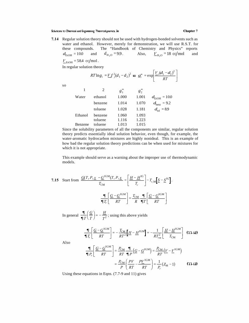
Solutions to Chemical and Engineering Thermodynamics, 3e Chapter 7
7.14 Regular solution theory should not be used with hydrogen-bonded solvents such aswater and ethanol. However, merely for demonstration, we will use R.S.T. forthese compounds. The “Handbook of Chemistry and Physics” reportsδEtOH = 100. and δH O2
= 9 9. . Also, V H O2cc mol= 18 and
V EtOH cc mol= 584. . In regular solution theory
RT Vi i jlnγ φ δ δ= −21 2
2a f so γδ δ
iiV
RT∞ =
−LNM
OQP
exp 1 22a f
so1 2 γ 1
∞ γ 2∞
Water ethanol 1.000 1.001 δEtOH = 100.
benzene 1.014 1.070 δbenz = 9 2.
toluene 1.028 1.181 δtol = 89.
Ethanol benzene 1.060 1.093toluene 1.116 1.223
Benzene toluene 1.013 1.015Since the solubility parameters of all the components are similar, regular solutiontheory predicts essentially ideal solution behavior, even though, for example, thewater-aromatic hydrocarbon mixtures are highly nonideal. This is an example ofhow bad the regular solution theory predictions can be when used for mixtures forwhich it is not appropriate.
This example should serve as a warning about the improper use of thermodynamicmodels.
7.15 Start from G T P x G T P x
T
H H
TT S S
cr
, , , ,,
( ) − ( ) = −LNM
OQP − −
IGM
CM
IG
MIG .
∂∂
∂∂T
G G
RT
T
R T
G G
RTr
−LNM
OQP = −L
NMOQP
IGMCM
IGM
In general ∂
∂T
G
T
H
TFH IK = − 2 ; using this above yields
∂∂T
G G
RT
T
RTH H
RT
H H
Tr rm
−LNM
OQP = − − = − −L
NMOQP
IGMCM IGM
IGM
CM2 2
1(7.7-12)
Also
∂∂
∂∂P
G G
RT
P
RT PG G
P
RTV V
P
P
PV
RT
PV
RT PZ
r
r
−LNM
OQP = − = −
= −FHG
IKJ = −
IGMCM IGM CM IGM
CMIGM
M
d i d i
a f11 (7.7-13)
Using these equations in Eqns. (7.7-9 and 11) gives

Solutions to Chemical and Engineering Thermodynamics, 3e Chapter 7
ln ln
ln
, ,
,
, ,
,
f
x P
f
P
T H H
RTN
T
N
PZ N
P
N
f
P
H H
RT T
Z
P
j
j
rm
j T P N
r
r
j T P N
r
j
r
j
i j
i j
= FHG
IKJ −
− FHG
IKJ
+ −FHG
IKJ
= FHG
IKJ −
−+ −
≠
≠
CMIGM
MM
IGM
M CM
M
d i
a f
d i a f
2
2 1 2
11
1
∂
∂
ψ ψ (7.7-14)
For Kay’s rules, T x Ti iCM C= ∑ , and P x Pi iCM C= ∑ , , we have
ψ∂∂
∂∂
∂∂
∂∂1 2 2
2 2
j r
j j j j
i i
j i ij
NT
NN
N
T
T
NT
T
T
N
NT
T N
N T
N
NT
T
T
N
N T
N
T
TT T
KCM CM
CM
CM
C
CM
C C
CM2 C CM
( ) =FHG
IKJ =
RSTUVW = − = −
RSTUVW
= − −RSTUVW = − −
∑
∑
,
, ,,m r
Since the “combining rule” for PCM is the same as for TCM (for Kay’s rule), it
follows that
ψ2 2j
jP
PP PK
CMC CM( ) = − −,m r
For the Prausnitz-Gunn rule, T TCM CM Kay= ( ) , so ψ ψ1 1j jPG K( ) = ( ) . However
P
R x Z x T
x V
i ii
i ii
i ii
CM
C C
C
=
FHG
IKJFHG
IKJ∑ ∑
∑, ,
,
Thus,
ψ∂∂
∂∂
∂∂
2 2
2
2
1
j r
j T P N j
j
i i i i
i i i
j i i
i i i
j i i
i i i i
j
i i
j
i
NP
N
NP
P NP
NP
P N
R N Z N T
N N V
NP
P
RZ N T
N N V
RT N Z
N N VP
N
V
N V
NP
P
Z
N Z
i j
PGCM
CM
CM
C C
C
CM
C C
C
C C
CCM
C
C
CM
C
C
( ) =FHG
IKJ = −
= −RST|
UVW|= − + − −
LNM
OQP
RST|UVW|
= −
≠
∑ ∑∑ ∑
∑∑ ∑
∑∑ ∑ ∑ ∑
, ,
, ,
,
, ,
,
, ,
,
,
,
,
k p
,
,
,
,
,
, , ,
i
j
i i
j
i i
j j j
T
N T N
V
N V
P
P
V
V
T
T
Z
Z
∑ ∑ ∑+ − −
RST|UVW|
= + − −RST
UVW
C
C
C
C
CM
C
CM
C
CM
C
CM
1
1
Thus
ψ2j j j jP
P
V V
V
T T
T
Z Z
ZPG
CM
C CM
CM
C CM
CM
C CM
CM
( ) =−F
HGIKJ −
−FHG
IKJ −
−FHG
IKJ
LNM
OQP
, , ,

Solutions to Chemical and Engineering Thermodynamics, 3e Chapter 7
7.16
System: 1 mole of initial mixturesystem is closed, isothermal and isobaric
Mass balance: x x1 2 1+ =
Energy balance: dU
dtQ P
dV
dtW= − +& &
s
Entropy balance: dS
dt
Q
TS= +
&&gen
Thus
& &
& &
& &
WdU
dtQ P
dV
dT
Q TdS
dtTS
WdU
dtT
dS
dtTS P
dV
dt
s
gen
s gen
= − +
= −
⇒ = − + +
a) Since both P and T are constant, we can write
& &
& &
WdU
dt
d
dtPV
d
dtTS TS
d
dtU PV TS TS
dG
dtTS
s gen
gen gen
= + ( ) − ( ) +
= + −( ) + = +
Clearly, for &Ws to be a minimum, &Sgen = 0 , and &WdG
dtsmin = .
W G G x G x G x G x G
x G G x G G
x RTf T P
f T P xx RT
f T P
f T P x
f ismin per mole of
initial mixtureFHG
IKJ = − = + − −
= − + −
=( )
( )+
( )( )
1 1 2 2 1 1 2 2
1 1 1 2 2 2
11
1
22
2
b g b gln
,
, ,ln
,
, ,
b) Now for either ideal mixtures or Lewis-Randall mixtures, f T P x
f T Pxi
ii
, ,
,
( )( )
= .
Therefore,
W RT x x x xsmin = − − ≥1 1 2 2 0ln ln , so work must be added!
T, Px1, x2
Process
T, Px1 moles pure 1
T, Px2 moles pure 2

Solutions to Chemical and Engineering Thermodynamics, 3e Chapter 7
[Note: & &Q TdS
dtTS= − gen ; thus & maxQ T
dS
dt= , which occurs when W Ws s
min= .
Following same analysis as above leads to
Q T x S T P S T P x x S T P S T P xmax , , , , , ,= ( ) − ( ) + ( ) − ( )1 1 1 2 2 2l qc) Using the ideal gas or ideal mixture assumption, since isomers can beexpected to form ideal mixtures, and the result above
W RT x x x xsmin J
mol K
J
mol K
J
mol of feed
= − − =⋅
× × − −
= −⋅
× × = −
1 1 2 2 8314 300 K 05 05 05 05
8 314 300 K 05 17288
ln ln . . ln . . ln .
. ln . .
7.17 NGN N
N NA
C N N
N N=
++ −
+
LNM
OQP
1 2
1 2
1 22
1 22
a fa f
GNG
Nx A C x x x x A C x x
x N CN N
N N
C N N
N N
x x A C x x x x C x x C x x
x A C x x Cx x x x x x
x A C
T P N
11
2 1 22
1 2 1 22
1 21 2
1 22
1 22
1 23
2 1 1 22
1 2 1 2 1 22
22
1 22
1 2 1 2 1 2
22
2
22
1 2 2
2 1
=( )
= + − − + −
+−+
−−
+LNM
OQP
= − + − + − − −
= + − + − − +
= +
∂∂ , ,
a f a fa fa f
a fa f
a f a f a f a fa f a fx x Cx x x x RT1 2
21 2
21 2 14− + − =a f a f lnγ
GNG
Nx A C x x x x A C x x
x x N NN N
N N
C N N
N N
x x A C x x x x C x x x x
x A C x x Cx x x x RT
T P N2
21 1 2
21 2 1 2
2
1 2 1 21 2
1 22
1 22
1 23
1 2 1 22
1 2 1 2 1 2
12
1 22
2 12
1 2 2
1
2 2
1 2 1
4
=( )
= + − − + −
+ + − −+
− −+
LNM
OQP
= − + − − − + −
= + − − − =
∂∂
γ
, ,
ln
a f a f
a f a fa f
a fa f
a f a f a fa f a f
or
RT x A C x x Cx x x
RT x A C x x Cx x x
ln
ln
γ
γ
1 22
1 22
1 1 2
2 12
1 22
2 1 2
4
4
= + − + −
= + − − −
a f a fa f a f
7.18 (a) i) One constant Margules equation.
RT A xlnγ1 121= −a f ; RT
xA x
∂ γ∂ln 1
112 1= − −a f

Solutions to Chemical and Engineering Thermodynamics, 3e Chapter 7
or
∂ γ∂
∂ γ∂
ln
limln
lim
1
1
1
1
1
1 1
1
2 1
2 10
1 1
x
A x
RT
x
A x
RTx x
= − −
=−
=→ →
a f
a f
ii) Two constant Margules equations
RT x x
x RTx x x
ln
ln
γ α β∂ γ∂
α β
1 1 12
1 13
1
11 1 1 1
21
1 1
12 1 3 1 0 as 1
= − + −
= − − − − → →
a f a fa f a fn s
iii) van Laar Equation
lnγ αα β1
1 221
=+ x xa f
Thus
∂ γ∂
α ββ α
ln 1
1
2 21
1 13 1
2 1
10 as 1
x
x
x xx= −
− +→ →a f
a fiv) Regular Solution Theory expression
R.S.T. has the same form as the van Laar Equation, so that proof followsfrom (iii) above.
(b) Starting from the Gibbs-Duhem Equation, Eqn. (7.3-16)
01
=FHG
IKJ=
∑ xxi
i
j T Pi
C ∂ γ∂ln
,
we obtain
0 11
12
2
1
= FHG
IKJ + F
HGIKJx
xx
xT P T P
∂ γ∂
∂ γ∂
ln ln
, ,
Alternatively, since dx dx2 1= − , we have
xx
xxT P T P
11
12
2
2
∂ γ∂
∂ γ∂
ln ln
, ,
FHG
IKJ = F
HGIKJ (*)
Now limx
x1 1
1 1→
= and limln
,x
T Px1 1
1
1
0→
FHG
IKJ =
∂ γ∂
⇒ FHG
IKJ = ⇒ F
HGIKJ =
→ →lim
lnlim
ln
, ,x
T Px
T P
xx
xx1 11
11
1 12
2
2
0 0∂ γ∂
∂ γ∂

Solutions to Chemical and Engineering Thermodynamics, 3e Chapter 7
which also implies that limln
,x
T P
xx2 0
22
2
0→
FHG
IKJ =
∂ γ∂
or, more generally
limln
,x
ii
i T Pi
xx→
FHG
IKJ =
00
∂ γ∂
Thus we have
limln
ln
,x
i
i T Pi
i xx
→
FHG
IKJ = ⇒
=1
1
0
1
∂ γ∂
γ departs, with
zero slope, from its
value of 0 at
and
limln
ln
.
ln,
xi
i
i T P ii
i i
i
xx x
x
x→
FHG
IKJ = ⇒ →
0
1
01
0∂ γ∂
γ
γ
rises less rapidly
than as Thus
is bounded!!!
7.19 Let M = molality of salt in solution.i) For KCl: z+ = 1 , z− = 1 , M MK = , M MCl = ;
I z M M M Mi i= = × + ×( ) =∑1
2
1
21 12
ii) For CrCl3 : z z
M M M MI M M M+ −
+ −
= = −= =
UVW = × + × =3 1
3
1
23 1 3 62 m r
iii) For Cr SO2 4 3a f : z z
M M M MI M M M+ −
+ −
= = −= =
UVW = × + × =3 2
2 3
1
23 2 4 3 152 m r
Now, the Debye-Hückel expression is lnγ α± + −= − z z Iand Equation (7.11-18)
ln .γ α±
+ −+ −= −
++z z I
Iz z I
101 ; α = FH IK1178
1 2
.mol
lit at 25°C
i) KClM lnγ ± Debye-Hückel Eqn. (7.11-18)
experiment ln .γ ± = −1178 Mln
..γ ± = −
++1178
101
M
MM
0.1 0.770 0.689 0.7610.2 0.718 0.590 0.7090.3 0.688 0.525 0.6790.5 0.649 0.435 0.6450.6 0.637 0.402 0.6350.8 0.618 0.349 0.6211.0 0.604 0.308 0.613

Solutions to Chemical and Engineering Thermodynamics, 3e Chapter 7
ii) CrCl3
M lnγ ± ln .γ ± = −8657 M ln
.
..γ± = −
++8657
1 2 44918
M
MM
0.1 0.331 0.065 0.2560.2 0.298 0.021 0.2260.3 0.294 87 10 3. × − 0.227
0.5 0.314 2 2 10 3. × − 0.2620.6 0.335 12 10 3. × − 0.291
0.8 0.397 4 3 10 4. × − 0.3731.0 0.481 17 10 4. × − 0.492
iii) Cr SO2 4 3a fM lnγ ± ln .γ ± = −27374 M
ln.
.γ± = −
++27374
1 38739
M
MM
0.1 0.0458 174 10 4. × − 0.0502
0.2 0.0300 4 82 10 6. × − 0.0113
0.3 0.0238 308 10 7. × − 0.1220.5 0.0190 392 10 9. × − 0.5080.6 0.0182 618 10 10. × − 1.104
0.8 0.0185 2 33 10 11. × − 5.559
1.0 0.0208 129 10 12. × − 29.44
Thus the Debye-Hückel and extended Debye-Hückel (with a fixed value ofthe δ parameter) theories are not very accurate. However, if the δ parameter isadjusted, much better agreement with experimental data can be achieved. Thisis left to the student to prove.
7.20 (also available as a Mathcad worksheet)

Solutions to Chemical and Engineering Thermodynamics, 3e Chapter 7
lngDH2i
1.178 Mi
0.5.
1 Mi
0.50.1 M
i.
lngDH3i
1.178 Mi
0.5.
1 Mi
0.50.30 M
i.

Solutions to Chemical and Engineering Thermodynamics, 3e Chapter 7
7.21 The Gibbs-Duhem equation, written in terms of molalities and using the meanionic activity coefficient is as follows: M dG M dG
G G RT M M
G G RT x
o
o
S S E E
E E
S S S S
is solvent and E is electrolyte
but
+ =
= +
= +
± + −+ −
0 where S
ln
ln
γ
γ
ν ν νc ha f
So that
M dG M dG
M d x M d M M
M d x M d M M d x M d M
S E E
S S S E
S S S E S S S E
S + =
+ =
+ = = +
± + −
± ± ± ±
+ −
0
0
0
ln ln
ln ln ln ln
γ γ
γ γ γ ν γ
ν ν ν
ν ν
a f c ha f c h a f d i
This is the Gibbs-Duhem equation for the solute-electrolyte system.
For HClM M+ = HCl ν+ = 1
M M− = HCl ν− = 1
M M M M± = ⋅ =2 2HCl1
HCl1
HCl
MS = =1000
185556.
xM
M M MSS
S E E
=+
=+
5556
5556
.
.
M d x M d MS S S HCl HClln lnγ γ+ +( ) =±1 1 0a f
d xM d M
M
d xM d M
xM
M
lnln
lnln
.
ln.
ln
γ γ
γγ
γ γ
S SHCl HCl
H O
S SHCl HCl
S SHCl
HCl
2
= −
=−
= −
±
±
±
2
2
5556
2
5556
a f
a f
a f∆ ∆
This can now be used as a basis for numerical integration with the activitycoefficient expression from Illustration 7.11-1. Or proceeding further,

Solutions to Chemical and Engineering Thermodynamics, 3e Chapter 7
d xM d M
M
d d xM d M d M
d dM
M d M d M
lnln
ln lnln
.
ln
.
ln ln.
.
ln
.
ln
.
γγ
γ γ
γγ
S SHCl HCl
H O
S SHCl HCl HCl
SHCl
HCl HCl HCl
2
=−
+ = − + −
++
FHG
IKJ = − +
−
±
±
±
2
2
5556
2
55565556
5556
2
5556
2
5556
a f
a f a f
a f a f
From Illustration 7.11-1
ln( ).
.γ± = −+
+1178
10 3
M
MMHCl
HClHCl
dM M M
dMln( ). .
( ).γ ± = −
++
++
FHG
IKJ
1
2
1178
1
1
2
1178
103
2HCl HCl HCl
HCl
ddM
M
M
M M MdM dM
ln.
.
. .
( ).
.
γ SHCl
HCl
HCl
HCl HCl HClHCl HCl
−+
= − −+
++
+FHG
IKJ −
5556
2
5556
1
2
1178
1
1
2
1178
103
2
55562
d
M
M
M
M
M
MdM
ln
.
.
. ( )
.
. ( )
.
. .
γ S
HCl
HCl
HCl
HCl
HCl
HClHCl=
++
⋅ +−
⋅ +− −
FHG
IKJ
1
5556
1178
5556 1
1178
5556 1
06
5556
2
55562
This can only be solved by numerical integration. (See MATHCAD file for thisproblem).
7.22 (a) The two-constant Redlich-Kister expansion, which leads to the two-constantMargules equation is
G x x A B x xex = + −1 2 1 2a fk p
1
4.5185 103.
gamma M( )
300 M0 10 20 30
0
0.5
1

Solutions to Chemical and Engineering Thermodynamics, 3e Chapter 7
Thus
G
x xA B x
ex
1 212 1= + −a f (1)
Which is a linear function of x.The form of the Wohl Equation which leads to the van Laar Equation is
GRTa x q x q
x q x qex =
+2 12 1 1 2 2
1 1 2 2
which can be rearranged to
x x
G
x q x q
RTa q q1 2 1 1 1 2
12 1 2
1
2ex =+ −a f
(2)
which is also a linear function of x. Equations (1) and (2) provide thejustification for the procedure.
(b) The figure below is the required plot. Clearly, neither equation is an accuratefit of the data. [The 2-constant Wohl (or van Laar) equation plot of the data,i.e., the form of Eq. (2), is closest to being linear, and therefore should be thebetter of the two-constant fits of the data. The data can, however, be fit quitewell with a 3-constant Redlich-Kister expansion—See Illustration 8.1-4]
7.23 Expression for Gex in this problem is the same as that of Eq. (7.6-6). If we
recognize that A and B in Eq. (7.6-6) is replaced by ART and BRT here. Also,
since 1 2− = −x x xAr CH Ar4a f c h , species 1 is methane and species 2 is argon.

Solutions to Chemical and Engineering Thermodynamics, 3e Chapter 7
(a) Therefore
RT ART BRT x BRTxlnγ 1 22
233 4= +( ) −
and
RT ART BRT x BRTxlnγ 2 22
233 4= −( ) +
At x x1 2 05= = .
ln . . .γ11
4
1
40 2944 0 0118 00766= +( ) = +( ) =A B ; γ CH 4
= 10796.
ln . . .γ21
4
1
402944 0 0118 00706= −( ) = −( ) =A B ; γAr = 10732.
(b) G RTx x A B xexAr Ar Ar= − + −1 1 2a f a fk p at xAr = 05.
G xART
Aex
Ar = =05.a f and G x
R
ATexAr =
=05
4
.a f
Thus
G x
RT
exAr at K K
==( ) = × =
05109 109
03036
48 2731
. ..
a f
G x
RT
exAr at K K
==( ) = × =
05112 112
0 2944
482432
. ..
a f
G x
RT
exAr at K K
==( ) = × =
05115 74 115 74
02804
481134
.. .
..
a f
Now replacing differentials with finite differences
T ∆T G
R
ex
∆ G
R
exFHG
IKJ
G
RT
ex
∆ G
RT
exFHG
IKJ
109 8.2731 0.07593 –0.0299 –0.0023
112 8.2432 0.07363.74 –0.1298 –0.0035
115.74 8.1134 0.0701
Next using
∂∂
∆ ∆G RT
T
H
RTP
a f =−
2 and ∂
∂
∆ ∆G RT
T
H
RT
H
RTP
ex exmixc hL
NMMOQPP
=−
=−
2 2
Thus ∆
∆∆
G RT
TRT H
ex
mix
c h b g× − =2 where T = average temperature over
∆T .

Solutions to Chemical and Engineering Thermodynamics, 3e Chapter 7
⇒ ≅ − × ( ) × − + −RSTUVW =∆H mix K J mol8 314 112
1
2
0 0023
3
00035
374888 2.
. .
..
(c) From ∂∂
G
TS
P
FHG
IKJ = − we obtain
∂∂T
G
R
S
RP
ex exFHG
IKJ = − . Therefore,
SR G R
Tex
ex
J mol K
J mol K
= − = − ×−
+−RST
UVW=
∆
∆
/.
. .
.
d i8 314
1
2
00299
3
01298
302213
Also
∆S R x x Si imixex
J mol K
= − + = − × × ( ) +
=∑ ln . . ln . .
.
8314 2 05 05 0045
5984
7.24 We start with
ln, ,
f
x P RTV V dP
RT
V
N
RT
PdPi
ii i
P
i T P N
P
j i
= − = FHG
IKJ −
LNMM
OQPPz z
≠
1 1
0 0
IGM
Eqn. (7.2-3a)
c h ∂∂
Now
dPV
d PVP
VdV
RT
VdZ
P
VdV
P
ZdZ
P
VdV= ( ) − = − = = −
1
Also, by triple product rule
∂∂
∂∂
∂∂
∂∂
∂∂
∂∂
V
N
P
V
N
P
VV
N
P
N
V
P
i T P N T N
i
T V N
ii P T N i T V N T N
j i j j i
j i j i j
FHG
IKJ ⋅ FHG
IKJ ⋅ FHG
IKJ = −
⇒ = FHG
IKJ = −FHG
IKJ
FHG
IKJ
≠ ≠
≠ ≠
, , , , ,
, , , , ,
1
So

Solutions to Chemical and Engineering Thermodynamics, 3e Chapter 7
ln
ln
, , ,
, ,
, ,
f
x P RT
P
N
V
PdP
P
P
ZdZ
P
VdV
RT
P
NNdV
VdV
ZdZ
RT
RT
VN
P
NdV
Z
Z
RT
RT
VN
P
N
i
i i T V N T N
i T V NV
V
V
V
PZ
Z
i T V NV
V
i
j i j
j i
j i
= −FHGIKJ
FHG
IKJ − −L
NMOQP
= − FHG
IKJ + −
= − FHG
IKJ
LNMM
OQPP −
=
= − FHG
IKJ
≠
≠
≠
z zz z z
z=∞ =∞ =
=
=∞
1 1
1 1 1
1
1
1
01
∂∂
∂∂
∂∂
∂∂
∂∂ T V NV
V
j i
dV Z, ,
ln≠
LNMM
OQPP −
=∞z
7.25
G
RTx x
G
RT
N G
RTN
x
N
G
RT N
G
RT
x
NN
N
N N
N
N
dN
dN
G
RTx
x
i j ijji
C
i
j ijj
i
C
T P N
j ijj
ij ij
ji
Ci
j ijj
j ijj
Ci i
j i
ex
ex ex
ex ex
ex
= −LNM
OQP
= = −L
NMMM
O
QPPP
⇒ =FHG
IKJ
= −
L
NMMM
O
QPPP
− −
L
NMMM
O
QPPP
= = −LNM
OQP
−
∑∑
∑∑
∑
∑∑∑
∑
=
=
=
=
≠
ln
ln
ln
ln ln
, ,
Λ
Λ
Λ
ΛΛ
Λ
ΛΛ
1
1
1
1
1
12
1
11
1
∂∂
γ 1
1 1
1
1
1
1
x
x x
x
xx
x
j ijj
i
C i j ijj
j ijj
i
C
j ijj
Ci i
j ijj
i
C
Λ
Λ
Λ
ΛΛ
Λ
∑∑∑
∑∑
∑ ∑∑
= =
= =
+
= −LNM
OQP
−ln
Which is the answer to part b... To obtain the result of part a, we restrict i and j tothe values 1 and 2, and note that Λii = 1 . Thus
ln lnγ1 1 2 121
1 2 12
2 21
1 21 2
1= − + −+
−+
x xx
x x
x
x xΛ
ΛΛ
Λbut
1 1
1 2 12
1 2 12 1
1 2 12
2 12
1 2 12
−+
=+ −
+=
+x
x x
x x x
x x
x
x xΛΛ
ΛΛ
Λso that
ln lnγ1 1 2 12 212
1 2 12
21
1 21 2
= − + ++
−+
LNM
OQPx x x
x x x xΛ
ΛΛ
ΛΛ

Solutions to Chemical and Engineering Thermodynamics, 3e Chapter 7
7.26 All the calculations for this problem were done using the program VLMU with thebinary interaction parameter for CO C2 4− n equal to 0.13 as given in Table 7.4-1.
The results are only given in graphical form here.
T = 377.6 Kkij = 0.13
80
supercriticalfCO2
60
40
vapor
2040
liquidvapor
fnC4
xnC4
80
60
60
4020

Solutions to Chemical and Engineering Thermodynamics, 3e Chapter 7
T =300 Kkij = 0.13
80
20
20
4040
60 liquid
liquidvapor
CO2f
fnC4
vapor
liquid
80
2040
60
40
20
xnC4

Solutions to Chemical and Engineering Thermodynamics, 3e Chapter 7
7.27
G ax x x x
NGAN N N N
N NA
N N N N
N N
ex
ex
= −
= −+
= −+
LNM
OQP
1 2 1 2
1 2 1 2
1 22
12
2 1 22
1 22
a fa f
a f a f∂
∂NG
NA
N N N
N N
N N N N
N N
A x x x x x x x
Ax x x x x x Ax x x x x x
Ax x x x x x Ax x Ax x
Ax x RT
N T P
ex
1
1 2 22
1 22
12
2 1 22
1 23
1 2 22
12
2 1 22
2 1 2 12
1 2 2 1 1 2 1 2
2 1 2 2 1 2 22
1 22
2
22
2
2
2 2
2 2 2
2 2 2 2 1 2
2 2 4 1 4 4 1
3 4
, ,
= −+
−−
+
LNMM
OQPP
= − − +
= − − + = − − +
= − + = − = − −
= − =
a fc ha f
a fa f
a f lnγ1
∂∂NG
NA
N N N
N N
N N N N
N N
A x x x x x x x
Ax x x x x x Ax x x x x x
Ax x x x x x Ax x Ax x
Ax x
N T P
ex
2
12
1 2
1 22
12
2 1 22
1 23
12
1 2 12
2 1 22
1 1 2 1 2 22
1 1 2 2 1 2
1 1 1 2 1 2 12
2 12
1
12
1
1
2 2
2 2 2
2 2 2 2 1 2
2 2 1 4 1 4 1
3 4
, ,
= −+
−−
+
LNMM
OQPP
= − − +
= − − + = + − −
= − − = − = − −
= − + =
a fc ha f
a fa f
a f RT lnγ2
(This is just a check since by symmetry of original equation 1 2↔ gives minussign. Therefore 1 2↔ on lnγ must give minus sign!)
Does this expression satisfy the Gibbs-Duhem Equation?
xd
dxx
d
dx11
12
1
1
0ln lnγ γ+ = or − + =x
d
dxx
d
dx11
22
1
1
0ln lnγ γ
d
dx
A
RT
d
dxx x
A
RT
d
dxx x
A
RTx x
d
dx
A
RT
d
dxx x
A
RT
d
dxx x
A
RTx x
ln
ln
γ
γ
2
1 112
11
12
13
1 12
1
2 222
22
22
23
2 22
3 4 3 4
6 12
3 4 3 4
6 12
= − + = − +
= − +
= − = −
= −
a f c h
c ha f c h
c hGibbs-Duhem Equation
− − + − +
= − + − +
= − + + = + −
xA
RTx x x
A
RTx x
A
RTx x x x x x x x
A
RTx x x x x x x x
A
RTx x x x
1 2 22
2 1 12
2 1 1 22
2 1 12
2
1 2 1 2 1 22
12
2 12
22
1 2
6 12 6 12
6 12 6 12
12 12 1212
1
c h c h
c h a f= ( ) =
120 01
222A
RTx x
⇒ Satisfies Gibbs-Duhem Equation

Solutions to Chemical and Engineering Thermodynamics, 3e Chapter 7
7.28 To check the utility of these models we will use the Gibbs-Duhem equation in theform
xx
xxT P T P
11
12
2
1
0∂ γ∂
∂ γ∂
ln ln
, ,
FHG
IKJ + F
HGIKJ =
For the model
ln
ln
γ
γ1 2
21
2
2 12
1= = −
=
Ax A x
Bx
a f
Gives
xx
xx
x A x x B x
x x B A
T P T P1
1
12
2
11 1 2 1
1 2
0 2 1 1 2
2 0
∂ γ∂
∂ γ∂
ln ln
, ,
FHG
IKJ +
FHG
IKJ = = ⋅ ⋅ − −( ) + ⋅
= −( ) =
a f
The only way this equation can be satisfied is if A B= ; if not the Gibbs-Duhemequation is violated.
For the model lnγ 1 2= Axn ; lnγ 2 1= Axn
xx
xx
x n A x x n Ax
nAx x x x
T P T P
n n
n n
11
12
2
11 1
12 1
1
1 2 22
12
1 1 0
0
∂ γ∂
∂ γ∂
ln ln
, ,
FHG
IKJ + F
HGIKJ = ⋅ ⋅ − −( ) + ⋅ ⋅ =
= − + =
− −
− −
a f
The only way the Gibbs-Duhem equation can be satisfied for all values of x1 and
x2 (with x x1 2 1+ = ) is if n = 2 in which case the term in brackets is always zero.
For the model lnγ 1 2= Axn ; lnγ 2 1= Bxn . We have
xx
xx
x n A x x n Bx
nx x Ax Bx
T P T P
n n
n n
11
12
2
11 1
12 1
1
1 2 22
12
1 1 0
0
∂ γ∂
∂ γ∂
ln ln
, ,
FHG
IKJ + F
HGIKJ = ⋅ ⋅ − −( ) + ⋅ ⋅ =
= − + =
− −
− −
a f
For this equation to be satisfied, the term in the brackets must be zero. This canonly be in n = 2 and A B= .

Solutions to Chemical and Engineering Thermodynamics, 3e Chapter 7
7.29 We will write the Flory-Huggins expression as
GRT
x mxx x m
x mx
G
RTN
xN
x
x
x mx
mx
x mx
G
RT
NG
RT
N N m
N mN
N
G
RT
N m
N mN
N N m
N mN
ex
res
ex
comb
ex
res
ex
res
ex
res
with
= + =+
= + =+
=+
= =+
FHG
IKJ =
+−
+= − = − =
χ φφ χ
φ φφ φ
χ
∂∂
χ χχ φ φφ χφ φ χφ
1 2 1 21 2
1 2
11
12
2
21
1
1 22
2
1 2
1 2
1 2
1
2
1 2
1 2
1 22 2 1 2 2 1 2
21
a f
a f a f a f
ln ln ,
Similarly
∂∂
χ χ χ φ φφ φ
φ φ
∂∂
φ ∂∂
φ ∂∂
φ
φ
N
G
RT
N m
N mN
N N m
N mNm xm
G
RTN
xN
x
N
G
RT xN
N xN
N x
x x mx
N
N mN
2
1
1 2
1 2
1 21 1 2 1
2
11
12
2
2
1
1
11
1
1
12
1
2
2
1
1 1 2 1 2
1
ex
res
ex
comb
ex
comb
FHG
IKJ =
+−
+= − =
= +
FHG
IKJ = + +
=+
=+
a f
ln ln
ln ln ln
and
∂∂
φ ∂∂
φ φ
φ
∂∂
φ ∂∂
φ φ
N x
N mN
N N mN
N
N mNN
N xx
x
m
x mx
Nm
N mN
N x
m
Nm N mNN
N xx
m
1
1
1
1 2
1 2 1 22 1
1
1
11 1
2
2 1 2 1 2
1
2
2 1 22
1
2
22
2
1
1
ln ; ln
ln ; ln
= ++
−+
LNM
OQP = −
=+
=+
= −+
LNM
OQP = −
a f
Therefore
ln
ln
ln ln
γ∂
∂∂
∂
φφ
φχφ
φφ
φφ
φφ χφ
11 1
1
11 1 2
222
1
11
222 1
12 2
21 11
=FHG
IKJ +
FHG
IKJ
= + − + −FH IK +
= + − − + = + −FH IK +
N
G
RT N
G
RT
xx x
m
x mx
x m
ex
comb
ex
res
a f
Also

Solutions to Chemical and Engineering Thermodynamics, 3e Chapter 7
∂∂
∂∂
φ φ
φφ
∂∂
φφ
∂∂
φ
γ φ φ φ χφ
φ φ φ φ φ φ χφ
φ φ
φ φ
N
G
RT NN
xN
x
xN
x
N xN
x
N x
xx m x
xm x
xm
xm
x m x
2 21
1
12
2
2
2
21
1
1 2
1
12
2
2 2
2
2
22
21 1 2 2 1
2
2
21 1 1
2 2
21 1
2
2
2
1 1 2 2
1
1
ex
conf
FHG
IKJ = +L
NMOQP
= + +
= + − + − +
= + − + = + −( ) +
= − −( )
− −
ln ln
ln
ln ln
ln ln
ln
1 244 344 1 244 344
a f a f
1 12+ χφ
7.30 (also available as a Mathcad worksheet)
7.30
i 0 1, 10.. xi
0.1 i.
fmai
xi
exp 1.06 1 xi
2.. 1.126.
fmi
1 xi
exp 1.06 xi
2.. 0.847.
x
0
0
1
2
3
4
5
6
7
8
9
10
0
0.1
0.2
0.3
0.4
0.5
0.6
0.7
0.8
0.9
1
= fma
0
0
1
2
3
4
5
6
7
8
9
10
0
0.266
0.444
0.568
0.66
0.734
0.8
0.867
0.94
1.024
1.126
= fm
0
0
1
2
3
4
5
6
7
8
9
10
0.847
0.77
0.707
0.652
0.602
0.552
0.496
0.427
0.334
0.2
0
=
Hma 1.126 exp 1.06( ). Hma 3.25=
Hm 0.847 exp 1.06( ). Hm 2.445=

Solutions to Chemical and Engineering Thermodynamics, 3e Chapter 7
7.31 Show A P Ca
bx
a
bii
iEOS
mix
mix
→ ∞( ) = −LNM
OQP∑
start − = → − = −→∞∞zP
A
VA A PdV
TV V
V∂∂
(V → ∞ is convenient since we have ideal gas and ideal gas mixtures)
P-R
PRT
V b
a
V V b b V b=
−−
+( ) + −( )← pure component
A ART
V b
a
V V b b V bdV
RT V ba
V bV bdV
V V
V V
V
− = −−
++( ) + −( )
= − −( ) − ∞ ++ −
→∞∞ ∞
∞
z zzln ln 2 22
Need to integrate1 2444 3444
From Problem 4.2 we have that
1
2
1
2 2
1 2
1 22 2V bV bdV
b
V b
V b
V
+ −=
+ −
+ +
FHG
IKJ∞
z lnd id i
⇒ − = − −( ) − ∞ ++ −
+ +
FHG
IKJ→∞A A RT V b
a
b
V b
V bV V ln ln ln2 2
1 2
1 2
d id i

Solutions to Chemical and Engineering Thermodynamics, 3e Chapter 7
So for pure component:
A A RT V ba
b
V b
V bi V i V ii
i
i
i
− = − − − ∞ ++ −
+ +
FHG
IKJ→ ∞ ln ln lna fk p d i
d i2 2
1 2
1 2
By exact analogy for mixture
A A RT V ba
b
V b
V bV V− = − − − ∞ ++ −
+ +
FHG
IKJ→∞ ln ln lnmix mix
mix
mix
mix mix
mix mix
a fk p d id i2 2
1 2
1 2
Now when V → ∞ get ideal gas or ideal gas mixture:
A A RT V ba
b
V b
V b
A A RT V b
a
b
V b
V b
V
V
− = − −( ) − ∞ ++ −
+ +
FHG
IKJ
− = − − − ∞
++ −
+ +
FHG
IKJ
IG
IGMmix mix
mix
mix
mix mix
mix mix
ln ln ln
ln ln
ln
2 2
1 2
1 2
2 2
1 2
1 2
d id i
a fk pd id i
and by definition A A Aex IM= − (i.e., A A A= +IM ex ) so; have A A− IGM so
A A A A Aex IGM IM IGM= − − +d i and
A x A RT x xi i i iIGM IG= +∑ ∑ ln ; A x A RT x xi i i i
IM = +∑ ∑ ln
A A A x A RT x x x A RT x x
A A A x A A
A
i i i i i i i i
i i i
ex IGM IG
ex IGM IG
this is why we found for pure component
= − − − + +
= − − −
∑∑ ∑ ∑∑
ln ln
d i d i∆
So putting in results for A A PdVV
V
− = −∞∞z for pure i and mixture.
A RT V ba
b
V b
V b
x RT V b RTa
b
V b
V bi i i
i
i
i i
i ii
exmix mix
mix
mix
mix mix
mix mix
= − − − ∞ ++ −
+ +
FHG
IKJ
− − − + ∞ ++ −
+ +
FHG
IKJ
RS|T|
UV|W|∑
ln ln ln
ln ln ln
a f d id i
a f d id i
2 2
1 2
1 2
2 2
1 2
1 2
Need to collect some terms.
A RT V b x V b
a
b
V b
V bx
a
b
V b
V b
i i ii
ii
i
i i
i i
exmix mix
mix
mix
mix mix
mix mix
= − − − ∞ − − − ∞LNM
OQP
+ −+ −
+ +
FHG
IKJ −
+ −
+ +
FHG
IKJ
∑
∑
ln ln ln ln
ln ln
a f a fd id i
d id i2 2
1 2
1 2 2 2
1 2
1 2
Now let P → ∞ which is the same as V bi i→ and V bmix mix→
= − − ∞ − − − ∞
+−
+
FHG
IKJ −
−
+
FHG
IKJ
∑
∑
RT b b x b b
a
b
b
bx
a
b
b
b
i i i
ii
i
i
i
[ ln ln [ ln ln ]
ln ln
mix mix
mix
mix
mix
mix
a f a fc hc h
c hc h
1 3 2 4
2 2
2 2
2 2 2 2
2 2
2 2
Now 1 and 2 cancel ln ln0 0 0− =∑ xi

Solutions to Chemical and Engineering Thermodynamics, 3e Chapter 7
and 3 and 4 cancel − ∞ + ∞ =∑ln lnxi 0 . i.e., −∞ + ⋅∞ =3 0
So
Aa
bx
a
b
ab
xab
Aa
bx
a
b
C P R
P RP
ii
i
ii
i
P RP
ii
i
-ex mix
mix
mix
mix
-ex mix
mix
where for -
→∞
→∞
= ⋅−+
FHG
IKJ −
−+
FHG
IKJ
= −+
FHG
IKJ ⋅ −L
NMOQP
= − −LNM
OQP
−+
FHG
IKJ = − =
∑
∑
∑
1
2 2
2 2
2 2 2 2
2 2
2 2
2 2
2 2
1
2 2
06232
2 2
2 2
1
2 20 6232
ln ln
ln
.
ln . *
Now for van der Waals ⇒ same process though solution is briefer.
− = ⇒ − = −−
+→∞ ∞ ∞z zPA
VA A
RT
V bdV
a
VdV
TV V
V V∂∂ 2
Pure component
A A RT V b RTa
V
A A RT V b RTa
V
A A A A A x A A
V i ii
i
V
i i
− = − − + ∞ −
− = − − + ∞ −
≡ − = − = − ←∑
IG
IGM
M MM
M
ex IM IGM IG
and for the mixture
and same as above
ln ln
ln ln
a f
a fd i d i
Putting in results for A A PdVV
V
− = −∞∞z for pure i and for the mixture.
A RT V b RTa
V
x RT V b RTa
V
RT V b x V b xa
Vx
a
V
M MM
M
i i ii
i
M M i i i iM
Mi
i
i
ex = − − − ∞ −
− − − − ∞ −RST
UVW= − − + − + ∞ − ∞ − +
∑
∑ ∑ ∑
ln ln
ln ln
ln ln ln ln
a f
a f
a f a f
Take limit P → ∞ , V bi i→ ; V bM M→ .
First 4 terms cancel!
Aa
bx
a
bP
M
Mi
i
iVDWex
→∞
= − −LNM
OQP∑1
7.32 Starting from
ba
RTx x b
a
RTQ
G Ca
bx
a
b
MM
iji
j ijij
ex M
Mi
i
ii
− = −FHG
IKJ ≡
= −LNM
OQP
∑∑
∑
and
*

Solutions to Chemical and Engineering Thermodynamics, 3e Chapter 7
or
and a
b
G
Cx
a
bDRT b
a
DRTM
M
ex
ii
iiM
M= + ≡ =∑*
Substituting, we then obtain
a
DRT
a
RTQ
a
RTQ
D
D
ba
RTQ Q
D
DQ
Q
D
M M M
MM
− = =−
= + =−
+ =−
so that
and1
1 1
7.33 Equation (7.10-11) is easily derived, is generic, and applies to any mixing rule.This will be used as the starting point. With the Wong-Sandler mixing ruleNote that derivatives must be taken with respect to mole numbers.
Therefore
needs to be in the form of
Similarly
needs to be in the form of
From this starting point, eqns. (7.10 -12 and 13) are easily derived.
Q x x ba
RT
N Q N N ba
RT
D xa
b RT
G
C RT
ND Na
b RTN G
C RT
i j ijij
ji
i j ijij
ji
ii
i
ex
i
ii
i
ex
i
= −FHG
IKJ
= −FHG
IKJ
= +
= +
∑∑
∑∑
∑
∑
2
*
*
7.34 Starting from eqn. (7.2-13)
ln ln, ,
/f
x P RT
RT
VN
P
NdV Zk
k k T V NV
V ZRT P
j k
= −∂
∂FHG
IKJ
LNMM
OQPP −
≠=∞
= z1
The Soave-Redlich-Kwong equation of state is
PRT
V b
a T
V V b
NRT
V Nb
N a T
V V Nb=
−−
+( )=
−−
+( )( ) ( )2
with
Nb N b N a N N ai ii
iji
j ij= =∑ ∑∑ and 2
Now taking the derivative, we obtain
RT
VN
P
N
RT
V
RT
V b
RTb
V b
x a
V V b
ab
V V bk T V N
ki ik
i k
j k
−∂∂
FHG
IKJ = −
−−
−( )+
+( )−
+( )≠
∑
, ,2 2
2
NP
NRT
V bRTb
V b
x a
V V bab
V V bk T V N
ki ik
i k
j k
∂∂
FHG
IKJ =
−+
−( )−
+( )+
+( )≠
∑
, ,2 2
2

Solutions to Chemical and Engineering Thermodynamics, 3e Chapter 7
and then
ln ln
ln/
/ /ln
/
/
/
ln
, ,
/f
x P RT
RT
VN
P
NdV Z
RT
RTZRT P
ZRT P b
RTb
ZRT P b
x a
b
ab
b
ZRT P
ZRT P b
ab
b ZRT P b
Z
k
k k T V NV
V ZRT P
ki ik
i k
k
j k
= − ∂∂
FHG
IKJ
LNMM
OQPP −
=−
+−
+ −RS|T|
UV|W| +
−+( )
L
N
MMMMMM
O
Q
PPPPPP
−
≠=∞
=
z∑
1
1
2
2
Now using B=Pb/RT and A = Pa/(RT)2 we obtain
ln ln ln lnf
x P
Z
Z B
B
Z B
A
B
x A
A
B
B
Z
Z B
A
B
B
Z BZk
k
ki ik
i k k=−
+−
+ −RS|T|
UV|W| +
−+
−∑
2
However, the Soave-Redlich-Kwong equation of state can be rewritten asfollows
PRT
V b
a
V V b
PV
RTZ
V
V b
a
RT V b
Z
Z B
A
Z B
ZB
Z B
A
Z B
=−
−+( )
= =−
−+( )
=−
−+
− =−
−+
1
Using this expression in the 2nd and 4th terms on the right-hand side of thefugacity expression yields the desired result
ln ln lnf
x PZ B
Z
Z B
A
B
x A
A
B
B
Z
Z B
B
BZk
k
i iki k k= − −
−+ −
RS|T|
UV|W| +
+ −( )∑
21
Note that in this derivation, we have used the followingdx
x x b b
x
x b
dx
x x b b
x
x b b x b
dx
x bx b
+( )=
+FH IK
+( )=
+FH IK +
+( )
−( )= −( )
zzz
1
1 12 2
ln
ln
ln
7.35 See Mathcad worksheet.a and b) See Mathcad file 7-35.MCD and figures contained there
c) Clearly

Solutions to Chemical and Engineering Thermodynamics, 3e Chapter 7
H RT x mxAx RT
Tx mx
x
x mx
mx
x mx
Ax x Rm
x mx
ex
= + = ++ +
=+
χ φφ1 2 1 22
1 21
1 2
2
1 2
22
1
1 2
a f a f a f a f
G
RTx
xx
x
Ax
Tx mx
RT
N G
N x m
NAxT
x mx
N
NAxT
x mx
N
A
T N
Nx x mx x mx
x mx
T P N
T P N
T P N
ex
ex
= + + +
= ∂∂
FHG
IKJ = + −FH IK +
∂ +FH IK∂
F
HGGG
I
KJJJ
∂ +FH IK∂
F
HGGG
I
KJJJ
=∂
∂++
11
12
2
2
21 2 1 2
11
1
12
21 2 1 2
1
21 2 1 2
1 1
2 1 2 1 2
1 2
11
1
2
2
2
ln ln
ln ln, ,
, ,
, ,
φ φ φφ
γ φ φφφ
φφ
a f
a f
a f a fa f a fa f
a fa f a f a f a fa f
21
2 1 2
1 2 1 2
2 2
1 2 1 2
2 1 2
1 22
1 2
2 1 2
1 2 1 22
2 2 2 2 1 1 2 22 2
1 12 2
2 1
11
1
1
11
LNM
OQP =
∂∂ + +
LNM
OQP
=+ +
−+ +
−+ +
LNM
OQP
= − − = − − = −
= + −F
A
T N
N N mN
N mN N N
A
T
N mN
N mN N N
N N mN
N mN N N
N N mN
N mN N N
AT
x x x xAx
Tx
AxT
x
x m
φ φ φ φ φ φ φ φ
γφ
ln ln H IK + −φφ
φ22 2
2 1Ax
Tx
ln ln, ,
, ,
, ,
γ φ φφφ
φφ
22
2
21
21 2 1 2
2
21 2 1 2
2 2
2 1 2 1 2
1 22
2
22
1
1 2 1 2
11
1
1
1
= ∂∂
FHG
IKJ = + −( ) +
∂ +FH IK∂
F
HGGG
I
KJJJ
∂ +FH IK∂
F
HGGG
I
KJJJ
=∂
∂++
LNM
OQP =
∂∂ + +
L
RT
NG
N xm
NAxT
x mx
N
NAx
Tx mx
N
A
T N
Nx x mx x mx
x mx
A
T N
N N m
N mN N N
T P N
T P N
T P N
ex a f
a f a fa f a fa fNM
OQP
=+ +
−+ +
−+ +
LNM
OQP
= − − = − − = +
= + −( ) + +
A
T
N mN
N mN N N
N N m
N mN N N
N N m
N mN N N
A
Tx x x x
Ax
Tx
Ax
Tx
xm
Ax
Tx
2
2 2
1
2 1
1 2 1 2
22
12
1 22
1 2
22
1
1 2 1 22
1 2 1 22
1 2 21 2
2 22 2
1 1
22
22
2 21 1
a fa f a f a f a fa fφ φ φ
φφ
φφ
γ φ φ φ φln ln
d) and e) See figures in Mathcad worksheet 7-35.mcd.

Solutions to Chemical and Engineering Thermodynamics, 3e Chapter 7

Solutions to Chemical and Engineering Thermodynamics, 3e Chapter 7

Solutions to Chemical and Engineering Thermodynamics, 3e Chapter 7

Solutions to Chemical and Engineering Thermodynamics, 3e Section 8.1
8
8.1-1 f f x P y PiV
iL
i i i i= ⇒ =vapγ , since the pressure is low enough that fugacity coefficient corrections
will be small.
(a) For the ideal solution, γ i = 1 for all species; 1 2= =EB nH, ; y x P Pi i i= vap . Thus,
y1 04723 07569 0 4537 07879= × =. . . .
and
y2 05277 00773 0 4537 00899= × =. . . . ;
yi∑ = 08778. which indicates that the ideal solution assumption is invalid!
(b) Regular solution behavior:
V V1 2
11 2
21 2
75 148 cm
8 9 7 4
= == =
cm
cal cc cal cc
3 3
δ δ. .a f a fφφ
1 1 1 1 1 2 2
2
0 4723 75 04723 75 05277 148 0312
0688
= + = × × + ×( ) ==
x V x V x Va f . . . .
.
ln .γφ δ δ
11 2
21 2 0133=
−=
V
RT; γ1 1142= . . Similarly γ2 1055= . . Therefore,
y1 1142 07879 08998= × =. . . ; y2 1055 00899 00948= × =. . . ; and yi∑ = 0 9946. which is much
closer to unity.(c) UNIFAC: using the program UNIFAC we have γ1 1173= . and γ2 1118= . ;
⇒ = × =y1 1173 07879 09242. . . ; y2 1118 00899 01005= × =. . . ; yi∑ = 10247. which is too high.
(d) First the expression γ i i iy P x P= 1vap and the given vapor-liquid equilibrium data will be used
to compute the species activity coefficients in the given solution:
γ108152 03197
0 2843 075691211=
××
=. .
. .. ; similarly, γ2 1069= .
Using eqns. (7.5-10) we obtain β = 03055. and α = 06747. . Thus, using the van Laar eqn.
ln.
.γ1
1 22
06747
1 2 2085=
+ x x and ln
.
.γ2
2 12
0 3055
1 0 4528=
+ x x
at x1 0 4723= . , γ1 1079= . , γ2 1144= . , so that y1 08504= . , y2 01029= . and yi∑ = 0953. .
Since none of the models yields yi∑ = 10. , none of the solution models is completely correct.

Solutions to Chemical and Engineering Thermodynamics, 3e Section 8.1
Since the regular solution model comes closest to meeting this criteria, it presumably leads tothe best predictions—however, this is merely a hypothesis.
8.1-2 The van Laar equation will be used to fit the data given. Starting from
γ i i i iy P x P= vap 1
2
==
H O
FURF2
we obtain, at 10 mole % water, γ1 5826= . and γ2 1266= . . Using eqn. (7.5-10) we get
α = 85648. and β = 07901. . Thus,
ln.
.γ1
1 22
85648
1 10841=
+ x xa f and ln.
.γ2
2 12
07901
1 00922=
+ x xa fwhich we will assume is valid at all temperatures.
At the new temperature we have x P y Pi i iγ 1vap = or x y1 1 110352 1013γ × = ×. . and
x y2 2 201193 1013γ × = ×. . which must be solved together with the activity coefficient expressions
above, and the criteria that x x1 2 1+ = and y y1 2 1+ = . Solution procedure I used was to guess a
value of x1 , compute x2 from x x2 11= − , compute γ1 and γ2 from the expression above, yi
from y x P Pi i i i= γ vap for i = 1 and 2, and then check to see if yi∑ = 1 . Proceeding this way,
the following results were obtained
calculated measured
x
x
y
y
1
2
1
2
0075 0 20
0925 080
0867 089
0129 011
. .
. .
. .
. .
Note yi∑ = 0.996 which is not quite equal to 1. The discrepancy between the calculated and
experimental results indicates the dangers of using approximate solution models.
8.1-3 The desired result may be proved a number of different ways.
Simplest proof: We have show that at an azeotropic point ∂∂
FHG
IKJ =P
x T1
0 using the triple product rule
in the form
∂∂
FHG
IKJ
∂∂
FH IK∂∂
FH IK = −P
x
T
P
x
TT x P1
1
1
1
yields
∂∂
FHG
IKJ = − ∂
∂FHG
IKJ
∂∂
FH IK =P
x
T
x
P
TT P x1 1 1
0
Since there is no reason to believe ∂∂
FH IK =P
T x1
0 in fact, vap∂
∂FH IK =
RSTUVW
P
T
P H
RTx12
∆

Solutions to Chemical and Engineering Thermodynamics, 3e Section 8.1
We then have ∂∂
FHG
IKJ =T
x P1
0 .
Alternate proof: P x P x P RT V= + =1 1 1 2 2 2γ γvap vap for an ideal gas phase. Thus
∂∂
FHG
IKJ = + ∂
∂+ ∂
∂LNM
OQP −
RST+ ∂
∂+ ∂
∂LNM
OQPUVW
=
T
x
V
RP x P
x
P
xP
x Px
P
x
P
P
11 1 1 1 1
1
1
1
12 2
2 2 22
1
2
1
0
γ γ γ γ
γ γ
vap vapvap
vap
vapvap
ln ln
ln ln
Now:
i)∂
∂FHG
IKJ =ln P
x P
1
1
0vap
Since the pure component vapor pressure does not depend on the mixture
composition at fixed P and T since ∂∂
FHG
IKJ =T
x P1
0
ii) Gibbs-Duhem eqn. is
H
T
T
xV
P
xx
xx
x
P P xx
ex
P
ex
P P P
P
∂∂
FHG
IKJ −
∂∂
FHG
IKJ +
∂∂
FHG
IKJ +
∂∂
FHG
IKJ =
⇒ − + ∂∂
FHG
IKJ
LNM
OQP =
→ →10
1
10
11
12
2
1
1 1 2 2 11
1
0
1 0
ln ln
ln
γ γ
γ γ γvap vapc h
or γ γ1 1 2 2P Pvap vap= . From here on it is the same argument as in the text.
Alternative to proof above: start with P x P x P= +1 1 1 2 2 2γ γvap vap
∂∂
FHG
IKJ ≡ = +
∂∂
FHG
IKJ +
∂∂
FHG
IKJ
RSTUVW −
+ ∂∂
FHG
IKJ + ∂
∂FHG
IKJ
RSTUVW
P
xP x P
x
P
xP
x Px
Px
P P P
P P
1
11 1 1 1 1
1
1
1
12 2
2 2 22
1
2
1
0 γ γγ
γ
γ γ
vap vapvap
vap
vapvap
ln ln
ln ln
Now using an argument similar to (i) above, and also using (ii), gives γ γ1 1 2 2P Pvap vap=
8.1-4 In general, we have x P y Pi i i iγ vap = and x P Pi i iγ∑ =vap . Also, from the experimental data, we
know PETvap = 02321. bar and PB
vap = 0 2939. bar.
(a) Ideal solution: x P y Pi i ivap = and x P Pi i∑ =vap . Thus y
x
PETET=
× 02321. and
P x x= × + =ET E02321 02939. . or P x= −02321 00617. . ET . Consequently x y− and P x−diagrams are given on following page.

Solutions to Chemical and Engineering Thermodynamics, 3e Section 8.1
(b) Regular solution model:
δi iV L
ethanol
benzene
125 584
9 2 890
. .
. .
Ethanol solubility parameters at 25°C was computed using ∆H ETvap = 9674 cal/mol
∆ ∆U H RTETvap
ETvap= − and δET ET
vapETL= ∆U Vd i1 2
Thus ln .γφ δ δ
φETB ET ET B
B=−
=2 2 2
210059V
RT and ln .γ φB ET= 15329 2 . These activity coefficient
expressions are used with the general equations above to obtain the solution. The results aregiven below.
(c) The program UNIFAC was used to obtain the predictions shown in the figures below.
(d) First we evaluate the activity coefficients at the given data point using γ i i i iy P x P= vap to
obtain γET = 12244. and γB = 20166. . Next using eqns. (7.5-10) we obtain α = 20271. and
β= 14993. . This is to be compared with α = 195. and β= 116. in Table 7.5-1]. Thus we
obtain
γ ETET ET
=+ −
RSTUVWexp
.
.
2 0271
1 13520 1 2x xa fand
γ BET ET
=+ −
RSTUVWexp
.
.
14993
1 0 7396 1 2x xa fUsing these expressions in the general equations we obtain the results plotted below.

Solutions to Chemical and Engineering Thermodynamics, 3e Section 8.1
8.1-5 (a) Using the vapor pressure data (Plotting ln Pvap vs 1 T ), I find that at T = °1054. C ,
PACvap ≈ 0 6665. bar and PT
vap ≈ 08793. bar. Thus γAC = =1013 0 6665 1520. . .a f and
γT = =1013 08793 1152. . . at the azeotropic composition of xT = 0 627. . Next, using eqns. (7.5-
10) and treating toluene as species 1, I find α = 1075. and β= 1029. . Thus,
ln.
.γT
T
M
=+
1075
1 10452x
x
and ln.
.γAC
AC
T
=+
1029
1 0 9572x
x
.
These expressions have been used to obtain the results plotted below.
(b) f f x P y PiL
iV
i i i i= ⇒ =γ vap . Thus, γ γi i i ix P P= vap and yi∑ = 1 . Procedure I used was, for
each value of xT , to
i) Guess an equilibrium temperature Tii) Compute yT and yAC , and check to see if yi∑ = 1
iii) If not, guess a new value of T and repeat the calculationA simpler procedure is to use Mathcad or another computer algebra program
Results Experiment van Laar IdealxT 0.25 0.50 0.75 0.25 0.50 0.75 0.25 0.50 0.75
yT 0.43 0.57 0.69 0.43 0.57 0.70 0.30 0.56 0.80
T °( )C 104.5 100.8 100.6 107.5 105.8 105.8 116.5 114 111
Ideal solution results were obtained in a similar matter, except that all activity coefficients wereset equal to unity.
8.1-5i 0 1, 20.. x
i0.05 i.
Write van Laar model this way to avoid division by zero.
gamt i( ) exp1.075 1 x
i2.
1 xi
1.045 xi
. 2gamac i( ) exp
1.029 xi
2.
xi
0.957 1 xi
. 2
gamt i( )
gamac i( )
xi
0 0.5 11
2
3
ln gamt i( )( )
ln gamac i( )( )
xi
0 0.5 10
0.5
1
1.5

Solutions to Chemical and Engineering Thermodynamics, 3e Section 8.1
8.1-6 (a) We start with eqn. (6.2-12b): x dG SdT VdPi i∑ + − = 0 . And note that at constant temperature
SdT = 0 and
dG RTd f RTd x f T Pi i i i i= =ln ln γ 1a fa f ,
so that
RT x d x RT x d RT x d f VdPi i i i i i∑ ∑ ∑+ + − =ln ln lnγ 0
However, for the pure fluid fugacity, we have, from eqn. (7.2-8a)
RTd f dG V dPi i iln = =
Thus
RT x d x RT x d x V V dPi i i i i i∑ ∑ ∑+ + − =ln lnγ b g 0
Also
x V V x V x V x V
V RT x d x V dP
i i i i i i i i
i i i
∑ ∑ ∑ ∑∑
− = − = −
= − ⇒ − =
ex
ex exln γa f 0
Now assuming
i) Ideal gas-phase behavior: x P y Pi i i iγ vap = or x y P Pi i i iγ = vap and
ii) That PV RTex / << 1 we obtain
x d x x d y P PPV
RTd Pi i i i i i∑ ∑= =ln ln lnγa f c hvap
ex
or
x d y x d P x d P PV RT d Pi i i i i∑ ∑ ∑+ − =ln ln ln lnvap exd i
Pi
xi
gamt i( ). 0.8793. 1 xi
gamac i( ). 0.6665. yi
xi
gamt i( ). 0.8793
Pi
.
Pidi
xi
0.8793. 1 xi
0.6665.yid
ixi
0.8793
Pidi
.
yi
yidi
xi
0 0.5 10
0.5
1
Pi
Pidi
xi
0 0.5 10.6
0.8
1

Solutions to Chemical and Engineering Thermodynamics, 3e Section 8.1
Now noting that x d Piivap∑ =ln 0 , since Pi
vap is a function of temperature only and
x d P d P x d Pi i∑ ∑= =ln ln lnb g , yields x d yPV
RTd Pii
ex
∑ = −FHG
IKJln ln1 or
x
ydy
x
ydy
x
y
x
ydy
PV
RTd P d P1
11
2
22
1
1
2
21 1+ = −F
HGIKJ = −
FHG
IKJ ≈ −
ex
ln ln
Since y y1 2 1+ = , dy dy2 1= − . Also y y2 1= − , and x x2 11= − ,
x
y
x
y
x y y x
y y
x y
y y1
1
1
1
1 1 1 1
1 1
1 1
1 1
1
1
1 1
1 1−
−−
=− − −
−=
−−
a f a f a fa f a f so
y x
y y
dy
dx
d P
dx1 1
1 1
1
1 11
−−
=a fa f
ln
To obtain the x y− diagram, I used the equation above in a finite difference form. Using
the argument i to denote the ith data point, the equation above becomes
y i x i
y i y iy i y i P i P i1 1
1 11 11
1 1( ) − ( )
( ) − ( )⋅ ( ) − −( ) = ( ) − −( )a f ln ln
y i1( ) is unknown, however, P i1( ) , P i1 1−( ) , x i1( ) are known. Also y1 1( ) is either 0 or 1
depending on which end of the data one starts with. In fact, I started at both ends, in twoseparate calculations, to check the results. I solved this problem using the equation aboverewritten as
y iB B C
1
2 4
2( ) =
± −
where
Bx i y i P
P=
( ) + −( ) ++
1 1 1
1
∆∆
ln
ln and C
x i y i
P=
( ) −( )+
1 1 1
1 ∆ ln
and averaged the results from starting at the x1 0= and x1 1= ends.
Once x1 and y1 , were known, the activity coefficients were calculated from
γ 1 1 1 1= y P x Pvap and γ 2 2 2 2= y P x Pvap . Results are given below.
b. CCl4 + n-Heptane System
= exprmntlx-y data

Solutions to Chemical and Engineering Thermodynamics, 3e Section 8.1
8.1-7 A simpler solution using Mathcad is available as a Mathcad worksheet.(a) At the bubble point we have
y x P Pi i i= vap where P = 5 bar
xET = 005. ; xP = 010. , xNB = 040. and xMP = 045. . Procedure used was
i) Guess T,ii) Compute each yi , and the sum yi∑ . If yi∑ = 1 , guessed T is correct; if yi∑ > 1 ,
guessed T is too high; if yi∑ < 1 , guessed T is too low. If yi∑ ≠ 1 , we correct T and
recalculate. Solution: T = 29366. K (bubble point) yET = 04167. , yP = 01730. ,
yNB = 01601. and yMP = 0 2502. .
(b) The dew point calculation is similar. Here, yET = 005. , yP = 010. , yNB = 040. and yMP = 045. .
P = 5 bar, and T and the xi 's are the unknowns. Thus, here we guess the dew point
temperature, compute each of the xi 's from x Py Pi i i= vap and evaluate xi∑ . If xi∑ = 1 , the
guessed temperature is the dew point temperature; if xi∑ >1 , guessed T is too low; if
xi∑ <1 , guessed T is too high. Solution (obtained using the computer) T = 314 23. K (dew
point) xET = 0 0039. , xP = 00337. , xNB = 05215. and xMP = 04409. .
(c) The advantage of the Mathcad worksheet for the isothermal flash calculation is that one can usethe initial flash equations directly, rather than having to make the substitutions below.
For the isothermal flash vaporization calculation, we proceed as in Illustration 8.1-3. First, wecalculate the K factors, i.e.
KET =+ − +
=10 817 08 303 15 4 402229
510185
. . ..
a f,
and, similarly KP = 2238. , KNB = 0546. and KMP = 0743. . Thus, the equations to be solved
are:x x x xET P NB MP+ + + = 1 (1)
y y y y x x x xET P NB MP ET P NB MP+ + + = ⇒ + + + =1 10185 2238 0546 0743 1. . . . (2)
Also,x L K K x LET ET ET ET1 0 05 10185 9185 005− + = ⇒ −( ) =a f . . . . (3)
and, similarly
c. Ethylene bromide + 1-nitropentane System
x-y data
Azeotrope
= exprmntl

Solutions to Chemical and Engineering Thermodynamics, 3e Section 8.1
x LP 2238 1238 010. . .−( ) = (4)
x LNB 0546 0454 0 40. . .+( ) = (5)
x LMP 0743 0257 0 45. . .+( ) = (6)
Solution procedure I used was to guess L, compute the xi 's from eqns. (3 to 6), and then
ascertain whether eqns. (1) and (2) were satisfied. After a number of iterations, I obtained thefollowing solution:
L
x
x
x
x
x
V
y
y
y
y
yi i
======
======∑ ∑
086667
00225
00858
04258
04659
1000
013333
0 2289
01921
0 2326
0 3464
1000
.
.
.
.
.
.
.
.
.
.
.
.
ET
P
NB
MP
ET
P
NB
MP
(d) For an adiabatic flush vaporization, shown below, the energy balance must also be satisfied
This is a (two-phase) Joule-Thomson expansion, so that the energy balance yields H Hin out= ,
or
x H T P x L x H T P x
V y H T P y
i iL
i iL
i iV
∑ ∑
∑
( ) = ( ) +, , , ,
, ,
inlet cond itions outlet liquid conditions
outlet vapor conditions c h
This equation must be satisfied, together with the mass balances and phase equilibriumequations of part c. Thus, we have one new unknown here, the outlet temperature, and anadditional equation from which to find that unknown.
8.1-8 (a) Starting from x P y Pi i i iγ vap = , we obtain γ i i i iy P x P= vap , and using the data in the problem
statement, we can compute each γ i , and then ln γ γP Aa f and G RT x xexP P A A= +ln lnγ γ .
These results, together with G RT x xexP A and its inverse are tabulated on the following page.
Also, there is a plot of ln γ γP Aa f vs. xA . This plot indicates that the data appears to be
thermodynamically consistent (i.e. lnz ≈γ γP A Aa fdx 0 ), though the points at the composition
extremes ( xA = 0021. and xA = 0953. ) look suspect
(b) See Problem 7.22 the plots of G RT x xexP A and x x G RTP A
ex appear on the following
page. The fact that neither is linear indicates that neither the two-constant Margules, nor the vanLaar equation will accurately fit the data. Hence, one will have to use at least a 3-constantRedlich-Kister expansion for the Gibbs free energy to obtain a good fit of the experimental datafor this system!
liquidliquid
vapor
X
pressure reducing valve or device

Solutions to Chemical and Engineering Thermodynamics, 3e Section 8.1
x xG
RT
G
RTx x
x x RT
GA P P Aγ γγγ
ln
. . . . . . . .
. . . . . . . .
. . . . . . . .
. . . . . . . .
. . . . . . . .
. . . . .
P
A
ex es
A P
A Pex
FHG
IKJ
0021 0979 33407 13140 09331 0 2927 14 237 00702
0061 0939 36497 10643 12323 01367 2 3866 04190
0134 0866 31326 11142 10337 0 2467 21259 04704
0 210 0 790 25617 11700 0 7837 0 3216 19385 05159
0 292 0 708 2 2196 12187 05995 0 3729 18037 05544
0405 0595 18190 13475 03000 0 4198 17421 05740
0503 0497 15132 15582 00293 0 4288 17153 05830
0611 0389 13299 18214 03145 0 4074 17141 05834
0 728 0272 11689 2 3716 07075 03485 17600 05682
0869 0131 10542 31505 10948 01962 17235 05802
0953 0047 10191 4 5509 14964 00893 19937 05016
. . .
. . . . . . . .
. . . . . . . .
. . . . . . . .
. . . . . . . .
. . . . . . . .
−−−−−
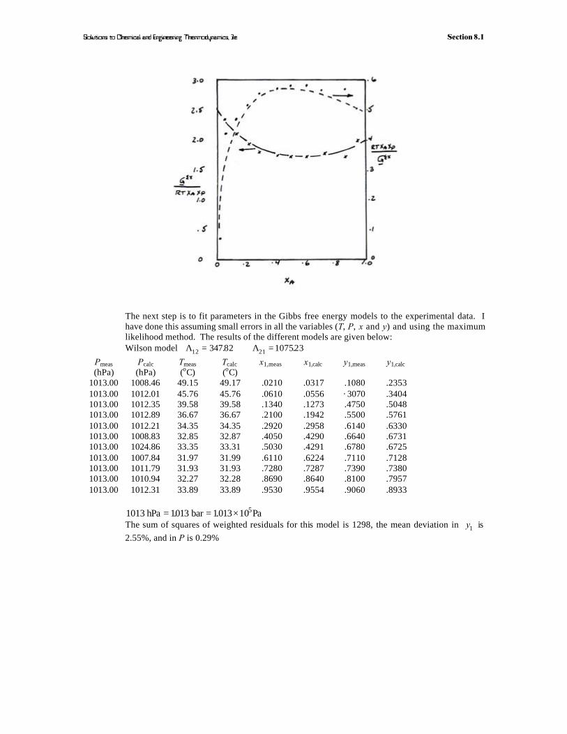
Solutions to Chemical and Engineering Thermodynamics, 3e Section 8.1
The next step is to fit parameters in the Gibbs free energy models to the experimental data. Ihave done this assuming small errors in all the variables (T, P, x and y) and using the maximumlikelihood method. The results of the different models are given below:Wilson model Λ12 347 82= . Λ21 107523= .
Pmeas
(hPa)Pcalc
(hPa)Tmeas
(oC)Tcalc
(oC) x1,meas x1,calc y1,meas y1,calc
1013.00 1008.46 49.15 49.17 .0210 .0317 .1080 .23531013.00 1012.01 45.76 45.76 .0610 .0556 · 3070 .34041013.00 1012.35 39.58 39.58 .1340 .1273 .4750 .50481013.00 1012.89 36.67 36.67 .2100 .1942 .5500 .57611013.00 1012.21 34.35 34.35 .2920 .2958 .6140 .63301013.00 1008.83 32.85 32.87 .4050 .4290 .6640 .67311013.00 1024.86 33.35 33.31 .5030 .4291 .6780 .67251013.00 1007.84 31.97 31.99 .6110 .6224 .7110 .71281013.00 1011.79 31.93 31.93 .7280 .7287 .7390 .73801013.00 1010.94 32.27 32.28 .8690 .8640 .8100 .79571013.00 1012.31 33.89 33.89 .9530 .9554 .9060 .8933
1013 1013 1013 105 hPa bar Pa= = ×. .The sum of squares of weighted residuals for this model is 1298, the mean deviation in y1 is
2.55%, and in P is 0.29%

Solutions to Chemical and Engineering Thermodynamics, 3e Section 8.1
NRTL model τ12 777 95= . τ21 432 53= .
Pmeas
(hPa)Pcalc
(hPa)Tmeas
(oC)Tcalc
(oC) x1,meas x1,calc y1,meas y1,calc
1013.00 1008.14 49.15 49.17 .0210 .0379 .1080 .24001013.00 1011.69 45.76 45.76 .0610 .0650 .3070 .34691013.00 1011.87 39.58 39.58 .1340 .1399 .4750 .51311013.00 1012.35 36.67 36.67 .2100 .2034 .5500 .58431013.00 1012.18 34.35 34.35 .2920 .2939 .6140 .64031013.00 1010.35 32.85 32.86 · 4050 .4186 .6640 .67931013.00 1025.99 33.35 33.30 .5030 .4173 .6780 .67841013.00 1007.37 31.97 31.99 .6110 .6208 ·7110 .71311013.00 1010.33 31.93 31.94 .7280 .7296 .7390 .73481013.00 1009.50 32.27 32.28 .8690 .8581 .8100 .78961013.00 1011.83 33.89 33.89 .9530 .9505 .9060 .8890
Sum of squares of weighted residuals =1547Mean deviation in y1 is 3.00%; in P = 0 34%.
UNIQUAC Model The parameters are τ12 = 572.61 and τ21 = –72.84Mean deviation in y1 is 3.0790; in P is 0.34%
Pmeas
(hPa)Pcalc
(hPa)Tmeas
(oC)Tcalc
(oC) x1,meas x1,calc y1,meas y1,calc
1013.00 1008.12 49.15 49.17 .0210 .0381 .1080 .24021013.00 1011.66 45.76 45.76 .0610 .0655 .3070 .34741013.00 1011.82 39.58 39.58 ·1340 .1412 .4750 .51411013.00 1012.26 36.67 36.67 .2100 .2048 .5500 .58551013.00 1012.10 34.35 34.35 ·2920 .2946 .6140 .64171013.00 1010.40 32.85 32.86 .4050 .4180 .6640 .68071013.00 1026.29 33.35 33.30 .5030 .4177 .6780 .68001013.00 1007.25 31-97 31.99 ·6110 .6206 .7110 .71391013.00 1010.16 31.93 31.94 .7280 .7295 .7390 .73511013.00 1009.43 32.27 32.28 .8690 .8579 .8100 .78951013.00 1011.80 33.89 33.89 .9530 .9503 .9060 .8888
van Laar modelα = 15032. β = 18534.
Mean % P = 0 34. ; y = 318%. sum of squares of wt. residuals =1625
Pmeas
(hPa)Pcalc
(hPa)Tmeas
(oC)Tcalc
(oC) x1,meas x1,calc y1,meas y1,calc
1013.00 1008.13 49.15 49.17 .0210 .0380 .1080 .24031013.00 1011.66 45.76 45.76 .0610 .0656 .3070 .34781013.00 1011.78 39.58 39.58 .1340 .1419 .4750 .51541013.00 1012.19 36.67 36.67 .2100 .2057 .5500 .58741013.00 1012.06 34.35 34.35 .2920 .2947 .6140 .64411013.00 1010.66 32.85 32.86 .4050 .4164 .6640 .68371013.00 1025.98 33.35 33.30 .5030 .4121 .6780 .68221013.00 1007.14 31.97 31.99 .6110 .6202 .7110 .71621013.00 1009.92 31.93 31.94 .7280 .7293 .7390 .73621013.00 1009.57 32.27 32.28 .8690 .8585 .8100 .78971013.00 1011.89 33.89 33.89 .9530 .9512 .9060 .8894

Solutions to Chemical and Engineering Thermodynamics, 3e Section 8.1
2-Constant Margules Model A = 17737. B = 19259.Mean % deviation in P = 0 33%. and in y = 2 90%. , and sum of squares of weighted residuals =1401
Pmeas
(hPa)Pcalc
(hPa)Tmeas
(oC)Tcalc
(oC) x1,meas x1,calc y1,meas y1,calc
1013.00 1008.60 49.15 49.17 .0210 .0287 .1080 .23371013.00 1012.14 45.76 45.76 .0610 .0502 .3070 .33821013.00 1012.66 39.58 39.58 .1340 .1135 .4750 .50221013.00 1013.56 36.67 36.67 .2100 .1731 .5500 .57361013.00 1013.81 34.35 34.35 .2920 .2764 .6140 .63141013.00 1004.67 32.85 32.88 .4050 .4396 .6640 .66531013.00 1023.95 33.35 33.31 .5030 .4598 .6780 .66701013.00 1005.18 31.97 32.00 .6110 .6465 .7110 .68991013.00 1014.78 31.93 31.92 .7280 .7317 .7390 .70821013.00 1013.07 32.27 32.27 .8690 .8863 .8100 .79321013.00 1012.36 33.89 33.89 .9530 .9578 .9060 .8928
So, of the models considered here, the Wilson model provides the best description (of the two-constant models) for this data set.
8.1-9 Using the program UNIFAC taking T and xP as known, and computing γ P , γA and P as well as
yP we obtain
x T P x P y yP Pcalc
Acalc calc
ibar
i ivap
Pcalc
PC°( ) =( )
∑γ γ γ exp
. . . . . . .
. . . . . . .
. . . . . . .
. . . . . . .
. . . . . . .
. . . . . . .
. . . .
0021 4915 41390 1006 0922 0147 0108
0061 4576 37515 10053 0 983 0325 0 307
0134 3958 31680 10258 0 976 0498 0475
0 210 3667 2 6687 10649 0 995 0583 0550
0 292 3435 2 2487 11302 0 993 0635 0 614
0405 3285 18162 12697 0 993 0677 0 664
0503 3335 15416 14540 1004 0697 0678
0611 3197 13247 17663 1002 0717 0711
0 728 3193 11592 2 3176 1001 0742 0 739
0869 3227 10388 35893 1005 0804 0810
0953 3389 10053 4 9909 1018 0897 0906
. . .
. . . . . . .
. . . . . . .
. . . . . . .
. . . . . . .
Ameasuredvalue =1013. bar

Solutions to Chemical and Engineering Thermodynamics, 3e Section 8.1
While the prediction is not perfect, it is relatively good.

Solutions to Chemical and Engineering Thermodynamics, 3e Section 8.1
8.1-10 First we should check to see if this problem is soluble (i.e.., well-posed in the sense of the Gibbsphase rule). The Gibbs phase rule, eqn. (6.9-6) is F C M P= − − + 2 . Thus here we haveF = − − + =3 0 2 2 3 degrees of freedom. Since the temperature, and two independent liquid-phase mole fractions are specified, the problem is well posed.
For the solution of this problem, the following subscripts will be used: 1 = ethanol ,2 = benzene and 3 = ethyl acetate . As the first step, compute the pure component vapor
pressures. This is done by using the vapor pressure data in the “Chemical Engineers' Handbook ”,
making plots of ln Pivap vs 1 T , and then determining ln Pi
vap (and hence Pivap ) at T = °78 C
1 2847 10 3T = × −. Kc h we find
P1 10vap ≅ . bar; P2 0 9666vap ≅ . bar and P3 1053vap ≅ . bar
Next, we need compute the liquid phase activity coefficients. This will be done using the ternaryvan Laar eqn. (eqn. (A7.3-2)). [See also Problem 7.8c], together with the entries in Table 7.6-1.Here one has to be careful about the order in which the species appear in the table. I obtained thefollowing:
α β α β β αα β α β β αα β α β β α
12 12 21 12 21 12
32 32 23 32 23 32
31 31 13 31 13 31
1946 1610 1610 1946
115 0 92 092 115
0896 0896 0896 0896
= = ⇒ = = = == = ⇒ = = = == = ⇒ = = = =
. . . .
. . . .
. . . .
Now from eqn. (A7.3-2)
ln
. . .
.
.
..
.
..
γα α α α α
γ
βα
βα
βα
βα
αβ
βα
βα
1
22
12
2
32
13
2
2 3 12 13 23
1 2 3
2
22
32
2 3
1 2 32
0 40 2
1
12
12
13
13
12
12
13
13
12
12
12
12
13
13
2 31
13320 0896 1730
08273
0 6333
0866607308
2 0767
=+ + + −
+ +
=+ +
+ += =
⇒ =
= ==
x x x x
x x x
x x x x
x x x x xx
e j e j e j e j e j
m r
To obtain an expression for γ2 , we interchange subscripts 1 and 2 in eqn. (A7.3-2) to obtain [see
solution to prob. 7.8c]
ln
. . .
. .
.
..
.
..
γβ α β α α
γ
αβ
βα
αβ
βα
βα
αβ
βα
2
12
12
2
32
23
2
1 3 12 23 13
2 1 3
2
12
32
1 3
2 1 32
0 40 2
2
12
12
23
23
12
12
23
23
12
12
12
12
23
23
2 31
2 3521 14375 2 7025
12087 1250
05403
130360 4145
15136
=+ + + −
+ +
=+ +
+ += =
⇒ =
= ==
x x x x
x x x
x x x x
x x x x xx
e j e j e je je j e j e j
m r
An expression for γ3 is obtained by interchanging indices 1 and 3 in eqn. (A7.3-2) to obtain [see
solution to Problem 7.8c]

Solutions to Chemical and Engineering Thermodynamics, 3e Section 8.1
ln
. . .
.
.
.
ln . .
..
γβ β β β β
γ γ
αβ
αβ
αβ
αβ
βα
αβ
αβ
3
22
23
2
12
13
2
1 2 23 13 12
3 2 1
2
22
12
1 2
3 2 12
0 40 2
3 3
23
23
13
13
23
23
13
13
23
23
23
23
13
13
2 31
0 7360 0896 00268
080
01557
08464
01840 and 12020
=+ + + −
+ +
=+ +
+ +=
⇒ = =
= ==
x x x x
x x x
x x x x
x x x x xx
e j e j e je je j e j e j
m r
With these "preliminaries" taken care of, we can now proceed on to the solution. The equilibriumequations are
x P y Pi i i iγ vap = and x P Pi i i∑ =γ vap
Therefore
x P
x P
x P
P
1 1 1
2 2 2
3 3 3
0 2 20767 1000 0 41534
04 15136 0 9666 058522
0 4 12020 1053 050620
150684
γ
γ
γ
vap
vap
vap
bar
bar
= × × =
= × × =
= × × ==
. . . .
. . . .
. . . .
.
and
y y y1 2 302756 03884 03360= = =. . .
Note that the vapor composition is only very slightly different than the liquid composition. (Thisis because the vapor pressures and activity coefficients of the species are all quite similar).
An alternative is to use the program UNIFAC to estimate the activity coefficients. Usingthe program with ethanol 1 CH , 1 CH , 1 OH3 2− − −a f , benzene (6–ACH) and ethyl acetate
1 CH , 1 CH , 1 CH COO3 2 3− − −a f we obtain, at 20 mole % ethanol, 40 mole % benzene and 40
mole % ethyl acetate at 78°C ) thatγ1 2 2062= . ; γ2 11931= . and γ3 10038= .
The solution is P = 12965. bar and
y1 03181= . ; y2 0 3558= . and y3 0 3261= .
Clearly this result is different from the ternary van Laar prediction. In the absence of experimentaldata for this ternary mixture, it is difficult to say which model is better.
8.1-11 For the simpler models, it is possible to show by simple mathematics that the model either does ordoes not permit a double azeotrope. For example, the van Laar model is
G
RT
a x q x q
x q x q
a
a
x x
x x
x x
x x
ex
=+
× =+
=−
+ −2 2
2
1
112 1 1 2 2
1 1 2 2
12
12
1 2
1 2
1 1
1 1
αβα β
αβα β
a fa f
Now for the benzene-hexafluorobenzene system Gex has an interior maximum and an interior
minimum. That is, dG dxex1 is zero twice in the region 0 11≤ ≤x . To see if the van Laar model
permits this we examine

Solutions to Chemical and Engineering Thermodynamics, 3e Section 8.1
d
dx
G
RT
x
x x
x
x x
x x
x x
exFHG
IKJ = −
+ −+ −( )
+ −− −
+ −−( ) =αβ
α βαβ
α βαβ
α βα β1
1
1
1
1
101
1 1
1
1 1
1 1
1 12
a fa fa f a f
a fa f
orαβ
α βαβ α β
β
α β α β
α α β β α β
1 2
1
1
10
0
0
1
1 1
1 1
1 12
2 1 1 2 1 2
1 2 12
1 2 22
1 2 1 2
−+ −
−− −( )
+ −=
⇒ − + − −( ) =
− − + − + =
x
x x
x x
dx x
x x x x x x
x x x x x x x x x x
a fa f
a fa f
a fa f
or
α βαβ
x xx
x12
22 2
1
2
= ⇒ =FHG
IKJ or
x
x2
1
= ±αβ
Now α β and must be of same sign (otherwise we get the square root of a negative number).
Also, since 0 11≤ ≤x and 0 12≤ ≤x , only positive sign is allowed. Thus x x2 1 = α β when
dG dxex1 0= . And only an interior maximum (if α > 0 and β > 0 ) or an interior minimum (if
α < 0 and β < 0 ) can occur, but not both! Therefore, van Laar model can not describe the
observed behavior.
Similarly, obviously the one-constant Margules model G Ax xex = 1 2 can not give both an interior
minimum & maximum, so it can not describe observed behavior.Instead of continuing this extreme argument, we will look at the results of merely fitting theexperimental data.
Two-constant-Margules model
Pmeas
(hPa)Pcalc
(hPa) x1,meas x1,calc y1,meas y1,calc
521.60 521.60 .0000 .0000 .0000 .0000525.70 518.42 .0941 .0940 .0970 .0880525.68 517.53 .1849 .1849 .1788 .1777522.87 517.19 .2741 .2741 .2567 .2679518.18 516.24 .3648 .3648 .3383 .3605509.89 514.09 .4538 .4539 .4237 .4522507.73 511.32 .5266 .5268 .4982 .5275503.50 507.72 .6013 .6015 .5783 .6051499.74 503.06 .6894 .6896 .6760 .6970497.57 498.70 .7852 .7852 .7824 .7960497.94 496.96 .8960 .8960 .8996 .9063501.55 501.55 1.0000 1.0000 1.0000 1.0000
- only 1 azeotrope at x1 09≥ .

Solutions to Chemical and Engineering Thermodynamics, 3e Section 8.1
Wilson model
Pmeas
(hPa)Pcalc
(hPa)y1,meas y1,calc
521.60 521.60 .0000 .0000525.70 510.55 .0970 .0757525.68 500.76 .1788 .1556522.87 492.21 .2567 .2407518.18 484.89 .3383 .3335509.89 479.35 .4237 .4300507.73 476.28 .4982 .5118503.50 474.74 .5783 .5974499.74 475.30 .6760 .6982497.57 479.24 .7824 .8038497.94 488.48 .8996 .9145501.55 501.55 1.0000 1.0000
Only a single azeotrope predicted to occur.
NRTL modelPmeas
(hPa)Pcalc
(hPa)x1,meas y1,meas y1,calc
521.60 521.60 .0000 .0000 .0000525.70 518.93 .0941 .0970 .0896525.68 516.49 .1849 .1788 .1773522.87 514.23 .2741 .2567 .2647518.18 512.08 .3648 .3383 .3545509.89 510.11 .4538 .4237 .4436507.73 508.62 .5266 .4982 .5170503.50 507.19 .6013 .5783 .5927499.74 505.66 .6894 .6760 .6825497.57 504.17 .7852 .7824 .7804497.94 502.69 .8960 .8996 .8938501.55 501.55 1.0000 1.0000 1.0000
No azeotrope results form the least squares fitting of parameters
UNIQUAC model
Pmeas
(hPa)Pcalc
(hPa)x1,meas y1,meas y1,calc
521.60 521.60 .0000 .0000 .0000525.70 528.19 .0941 .0970 .0953525.68 526.27 .1849 .1788 .1717522.87 521.58 .2741 .2567 .2503518.18 515.87 .3648 .3383 .3368 ←509.89 510.44 .4538 .4237 .4276507.73 506.61 .5266 .4982 .5046503 50 503.46 .6013 .5783 .5852499.74 500.91 .6894 .6760 .6807497.57 499.57 .7852 .7824 .7832497.94 499.80 .8960 .8996 .8978 ←501.55 501.55 1.0000 1.0000 1.0000
Double azeotrope predicted, as indicated.

Solutions to Chemical and Engineering Thermodynamics, 3e Section 8.1
Therefore, of the models considered only the UNIQUAC model is capable of producing the
peculiar behavior of Gex for this system.
8.1-12 From Table 8.1-1 we have (assuming an ideal vapor phase)
x1 1 2 101
200503 34337 10247 05251
01014 31394 10192 04885
01647 2 6218 10445 0 3997
0 2212 2 2340 10918 0 3109
0 3019 19334 11332 02320
0 3476 17879 11637 01865
0 4082 15928 12643 01003
04463 15237 13068 00666
05031 14284 13755 0 0164
05610 13225 14984 0 0542
0 6812 11841 17837 01779
0 7597 11285 2 0086 0 2504
08333
γ γγγ
log
. . . .
. . . .
. . . .
. . . .
. . . .
. . . .
. . . .
. . . .
. . . .
. . . .
. . . .
. . . .
.
FHG
IKJ
−−−
10648 2 4539 03625
0 9180 10223 31792 0 4927
. . .
. . . .
−−
See figure below.

Solutions to Chemical and Engineering Thermodynamics, 3e Section 8.1
Log
The two areas I and II appear to be approximatelyequal, so the data will be presumed to bethermodynamically consistent. In fact, from propernumerical analysis, we find the data to be consistent.

Solutions to Chemical and Engineering Thermodynamics, 3e Section 8.1
8.1-13P x P x P= +1 1 1 2 2 2γ γvap vap
∂∂
FHG
IKJ = − + ∂
∂+ + ∂
∂P
xP x P
xP x P
xT21 1 1 1
1
22 2 2 2
2
2
γ γ γ γvap vap vap vap ; where we have used that ∂∂
= −x
x1
2
1 as
x2 10 1→ →γ and ∂∂
=γ1
2
0x
. So
∂∂
FHG
IKJ = − + +
→
P
xP P
T x2 01 2 2
2,
vap vapγ xx2
2
2
0→( ) ∂∂γ
so that
γ2 2
1
0
2
02 2x
P Px
PT x→ =
+ ∂∂
FHG
IKJ
→a fvap
vap, constant temperature ebulliometer
Now
P x P x P= +1 1 1 2 2 2γ γvap vap
and
∂∂
FHG
IKJ = = − + ∂
∂FHG
IKJ + ∂
∂FHG
IKJ
∂∂
FHG
IKJ
+ +∂∂
FHG
IKJ +
∂∂
FHG
IKJ
∂∂
FHG
IKJ
P
xP x
xP x
P
T
T
x
P xx
P xP
T
T
x
P P P
P T P
21 1 1
1
21 1 1
1
2
2 2 22
22 2 2
2
2
0 γ γ γ
γγ
γ
vap vapvap
vap vapvap
as x2 10 1→ →, γ and ∂∂
→γ1
2
0x
0 011
22 2 2= − + ∂
∂FHG
IKJ + →P
dP
dT
T
xx P
P
vapvap
vapγ a f
or
γ2 2
11
0
2
02 2x
PdP
dTTx
PP x→ =
− FHGIKJ ∂
∂FHG
IKJ
→a fvap
vap
vap, constant pressure ebulliometer
8.1-14 (also available as a Mathcad worksheet)Clearly many different thermodynamic models can be used. We will use the van Laar model
lnγ ααβ
1 21 1
2
=+ x
x
and lnγ ββα
2 21 2
1
=+ x
x
which gives lnγ α1∞ = and lnγ β2
∞ = . Using the data in the problem statement
α = ( ) =ln . .16931 05266 and β= ( ) =ln . .19523 0 6690 . Using these parameter values in the activity

Solutions to Chemical and Engineering Thermodynamics, 3e Section 8.1
coefficient equations above, together with P x Pi i i i= γ vap ; P P P= +1 2 and y P Pi i= gives, at
x1 02= .
x y y2 1 202 04483 05517= = =. . . and P = 06482. bar
Also
x y y P2 1 20500 0 7036 0 2946 08431
0 700 08118 01882 09262
0850 08943 01057 09732
0 900 0 9256 00744 09861
0 950 09604 0 0396 09972
0975 09795 00205 10019
= = = =. . . .
. . . .
. . . .
. . . .
. . . .
. . . .
8.1-15 (also available as a Mathcad worksheet)Using Mathcad I obtained the following results
T K T K
x x
= == =
− −300 K 400 K
01 58340 01 15318
05 0 4255 05 11172
09 003103 0 9 00815
EOH EAC EOH EAC
EOH EOH. . . .
. . . .
. . . .
Thus the results exhibit strong composition and temperature dependence. For an ideal solution
x P y Py
x
P
PK
y x
y x
P
Pi i ii
i
iij
i i
j j
i
j
vapvap vap
vap= ⇒ = ⇒ = =
Thus, for an ideal solution, the relative volatility Kij has no composition dependence, but can be
dependent on temperature (unless, fortuitously, Pivap and Pj
vap have the same temperature
dependence, that is, ∆ ∆H Hi jvap vap= ). The composition dependence arises from the non-ideal
solution behavior. Since the activity coefficients dependent on temperature, nonideal solutionbehavior also contributes to the temperature dependence of the relative volatility.
8.1-16 This system was used for illustration in the first edition. The figures which appear below are fromthat source. [I changed to the hexane-triethylamine system since the x and y were too close in thebenzene-ethylene chloride system because the pure component vapor pressures are so close.]

Solutions to Chemical and Engineering Thermodynamics, 3e Section 8.1
8.1-17
x Pf
Py P1 1 1 1γ vapFH IK =
(a) αγγ
γγ21
2 2
1 1
2 2 2
1 1 1
2 2 2
1 1 1
2
1
2
1
1 2
1
1 2
12
22
12
22
12
12
1
= = = =
= =
=
− − −
− −
y x
y x
P f P P
P f P P
P f P
P f P
P e f P
P e f P
P
Pe
f P
f P
P
Pe
f P
f P
P
Pe
Ax RT
Ax RT
A x x RT A x x RT
T
A x RT
T
vap
vap
vap
vap2vap
1vap
2vap
1vap
2vap
1vap
2vap
1vap
dependence
Compositionand dependence
a fa f
a fa f
a fa f
a fa f
a fa f
;
d i a fd i
a f1 24 34
124 34
f P
f PT P
a fa f
2
1
and dependence
(b) Ideal mixture at low pressure
A = 0 above and also all f
PFH IK = 1
α212
1
= ( )( )
P T
P TT
vap
vap
dependence124 34

Solutions to Chemical and Engineering Thermodynamics, 3e Section 8.1
8.1-18 a) Starting from
f f x P y P
x P x P P
yx P
x P x P
y xP
P P
i
L
i
L
i i i
ii i
ii
= =
+ =
=+
= =+
we get, for the ideal solution, that
Now adding such equations for both components, we get
so that
In a equimolar mixture
vap
vap vap
vap
vap vap
vap
vap vap
1 1 2 2
1 1 2 2
11 2
05
;
.a f
b) For the nonideal mixture
Now adding these equations for both components, we get
so that
For the one - constant Margules model
In a equimolar mixture with the
vap
vap vap
vap
vap vap
vap
vap vap
vap
vap vap
x P y P
x P x P P
yx P
x P x P
yx P a x
x P ax x P ax
y xP a
P a P a
i i i i
ii i i
ii i i
ii
γ
γ γ
γγ γ
=
+ =
=+
=−
+
= =( )
( ) + ( )
1 1 1 2 2 2
1 1 1 2 2 2
2
1 1 22
2 2 12
1
2
12
2
1
0505 05
05 05 05 05
;
exp( )
exp( ) exp( )
.. exp( . )
. exp( . ) . exp( .
a f
a f 21 2)
=+
P
P Pivap
vap vap
which is exactly the same result as for the ideal solution. However, these twodifferent models only give the same vapor-phase composition in an equimolarmixture. However, even in this case, the pressures for the ideal and one-constant Margules mixtures are different.
8.1-19
G Ax xAx
RTex = ⇒ =
FHG
IKJ1 2 1
22
γ exp ; γ212
=FHG
IKJexp
Ax
RT
x P y P1 1 1 1γ vap =
Azeotrope x yP
P1 1 11
= ⇒ =γ vap
γγ
2
1 2
1 1
2
12
22
12
22
= ⋅ = = = −P
P
P
P
P
P
e
ee
Ax RT
Ax RT
A x x RT
vap
vap vap
vapd i
ln
ln ln ln
P
P
A
RTx x
A
RTx x
A
RTx x x
A
RTx
P
PA
RT
x
P
P
RT
x
P
P
1
212
22
12
12
12
1 12
11
2 1
1
2 1
2
1
1 1 2
2 12 1 1 2
vap
vap
vap
vap
vap
vap
vap
vap
= − = − − = − + −
− = ⇒ =−
=−
c h a fd i c h
a fSo for an azeotrope to form
(1) If P P2 1vap vap>
Azeotrope will form near x1 0= if A RTP
P= ln 2
1
vap
vap
Azeotrope will form at x1 05+ = . if A = ∞ ; at x1 05− = . if A = −∞ .

Solutions to Chemical and Engineering Thermodynamics, 3e Section 8.1
Azeotrope will form near x1 1= if A RTP
P= − ln 2
1
vap
vap
Or in general xRT
A
P
P12
1
1
21= −
FHG
IKJ
FHG
IKJln
vap
vap
So we can draw figures of regions in which azeotropes can be expected to form.
(2) If P P1 2vap vap> then A
RT
x
P
P=
−1 2 1
1
2
lnvap
vap
Mirror image of point 1
(b) TAx x
R=
−2 11 1a f; A
RT
x x=
−2 11 1a f at x1 05= . ; A RT= 2
8.1-20 (also available as a Mathcad worksheet)
8.1-20
T 69
p5 10.42226799
8.314 273.15 T( ). p5 exp p5( ) p5 2.721=
p6 10.45629676
8.314 273.15 T( ). p6 exp p6( ) p6 1.024=
p7 11.43135200
8.314 273.15 T( ). p7 exp p7( ) p7 0.389=
x5 0.25 x6 0.45 x7 0.3
P x5 p5. x6 p6. x7 p7. P 1.258=
y5x5 p5.( )
Py6
x6 p6.( )
Py7
x7 p7.( )
P
Bubble point pressure P 1.258=
Bubble point compositions y5 0.541= y6 0.366= y7 0.093=
Now on to dew point calculation
Initial guesses P 1 x5 0.1 x6 0.6 x7 0.3
z5 0.25 z6 0.45 z7 0.3
GIVENx5 x6 x7 1 x5 p5. z5 P. x6 p6. z6 P. x7 p7. z7 P.
soln FIND x5 x6, x7, P,( )
x5 soln0
x6 soln1
x7 soln2
P soln3
Dew point pressure P 0.768=
Dew point compositions x5 0.071= x6 0.338= x7 0.592=

Solutions to Chemical and Engineering Thermodynamics, 3e Section 8.1
8.1-21 (also available as a Mathcad worksheet)
8.1-21
Solving for the bubble point pressure
T 69 P 1.013
p5 T( ) exp 10.42226799
8.314 273.15 T( ).p5 T( ) 2.721= K5 T P,( )
p5 T( )
P
p6 T( ) exp 10.45629676
8.314 273.15 T( ).p6 T( ) 1.024= K6 T P,( )
p6 T( )
P
p7 T( ) exp 11.43135200
8.314 273.15 T( ). p7 T( ) 0.389= K7 T P,( )p7 T( )
P
y5 0.33 y6 0.33 y7 0.33 z5 0.25 z6 0.45 z7 0.3
GIVEN
K5 T P,( ) z5. K6 T P,( ) z6. K7 T P,( ) z7. 1 y5 K5 T P,( ) z5. y6 K6 T P,( ) z6. y7 K7 T P,( ) z7.
soln FIND y5 y6, y7, P,( )
y5 soln0
y6 soln1
y7 soln2
P soln3
y5 0.541= y6 0.366= y7 0.093= P 1.258=
This is the bubble-point pressure solution. Now on to the dew-point pressure problem.
Note that xi=yi/Kix5 0.33 x6 0.33 x7 0.33
GIVEN
z5
K5 T P,( )
z6
K6 T P,( )
z7
K7 T P,( )1 x5
z5
K5 T P,( )x6
z6
K6 T P,( )x7
z7
K7 T P,( )
soln FIND x5 x6, x7, P,( )
x5 soln0
x6 soln1
x7 soln2
P soln3
x5 0.071= x6 0.338= x7 0.592= P 0.768=
This is the dew-point pressure solution.So for a mixture of the composition z5=0.25, z6=0.45 and z7=0.30, at a temperature of 69 C, the mixture will be all liquid at pressures above 1.258 bar, and all vapor at pressures below 0.768 bar. Vapor-liquid equilibrium will exist at this temperature only between 0.768 and 1.258 bar, so this is the pressure range we will examine.

Solutions to Chemical and Engineering Thermodynamics, 3e Section 8.1
T 69 L 0.99 P 1.2
GIVEN K5 T P,( ) x5. K6 T P,( ) x6. K7 T P,( ) x7. x5 x6 x7( ) 0
x5 L 1 K5 T P,( )( ). K5 T P,( )( ). z5
x6 L 1 K6 T P,( )( ). K6 T P,( )( ). z6
x7 L 1 K7 T P,( )( ). K7 T P,( )( ). z7 soln FIND x5 x6, x7, L,( )
x5 soln0
x6 soln1
x7 soln2
L soln3
V 1 L
x5 0.223= x6 0.456= x7 0.32= V 0.094= L 0.906=
y5 K5 T P,( ) x5. y6 K6 T P,( ) x6. y7 K7 T P,( ) x7.
y5 0.507= y6 0.389= y7 0.104=
P 1.1L 0.80
GIVEN K5 T P,( ) x5. K6 T P,( ) x6. K7 T P,( ) x7. x5 x6 x7( ) 0
x5 L 1 K5 T P,( )( ). K5 T P,( )( ). z5
x6 L 1 K6 T P,( )( ). K6 T P,( )( ). z6
x7 L 1 K7 T P,( )( ). K7 T P,( )( ). z7 soln FIND x5 x6, x7, L,( )
x5 soln0
x6 soln1
x7 soln2
L soln3
V 1 L
x5 0.18= x6 0.458= x7 0.362= V 0.264= L 0.736=
y5 K5 T P,( ) x5. y6 K6 T P,( ) x6. y7 K7 T P,( ) x7.
y5 0.445= y6 0.427= y7 0.128=
P 1.0 L 0.60
GIVEN K5 T P,( ) x5. K6 T P,( ) x6. K7 T P,( ) x7. x5 x6 x7( ) 0
x5 L 1 K5 T P,( )( ). K5 T P,( )( ). z5
x6 L 1 K6 T P,( )( ). K6 T P,( )( ). z6
x7 L 1 K7 T P,( )( ). K7 T P,( )( ). z7 soln FIND x5 x6, x7, L,( )
x5 soln0
x6 soln1
x7 soln2
L soln3
V 1 L
x5 0.141= x6 0.445= x7 0.414= V 0.451= L 0.549=
y5 K5 T P,( ) x5. y6 K6 T P,( ) x6. y7 K7 T P,( ) x7.
y5 0.383= y6 0.456= y7 0.161=

Solutions to Chemical and Engineering Thermodynamics, 3e Section 8.1
P 0.9 L 0.40
GIVEN K5 T P,( ) x5. K6 T P,( ) x6. K7 T P,( ) x7. x5 x6 x7( ) 0
x5 L 1 K5 T P,( )( ). K5 T P,( )( ). z5
x6 L 1 K6 T P,( )( ). K6 T P,( )( ). z6
x7 L 1 K7 T P,( )( ). K7 T P,( )( ). z7 soln FIND x5 x6, x7, L,( )
x5 soln0
x6 soln1
x7 soln2
L soln3
V 1 L
x5 0.107= x6 0.412= x7 0.481= V 0.663= L 0.337=
y5 K5 T P,( ) x5. y6 K6 T P,( ) x6. y7 K7 T P,( ) x7.
y5 0.323= y6 0.469= y7 0.208=
P 0.8 L 0.20
GIVEN K5 T P,( ) x5. K6 T P,( ) x6. K7 T P,( ) x7. x5 x6 x7( ) 0
x5 L 1 K5 T P,( )( ). K5 T P,( )( ). z5
x6 L 1 K6 T P,( )( ). K6 T P,( )( ). z6
x7 L 1 K7 T P,( )( ). K7 T P,( )( ). z7 soln FIND x5 x6, x7, L,( )
x5 soln0
x6 soln1
x7 soln2
L soln3
V 1 L
x5 0.078= x6 0.359= x7 0.563= V 0.91= L 0.09=
y5 K5 T P,( ) x5. y6 K6 T P,( ) x6. y7 K7 T P,( ) x7.
y5 0.267= y6 0.459= y7 0.274=
P 0.77 L 0.10
GIVEN K5 T P,( ) x5. K6 T P,( ) x6. K7 T P,( ) x7. x5 x6 x7( ) 0
x5 L 1 K5 T P,( )( ). K5 T P,( )( ). z5
x6 L 1 K6 T P,( )( ). K6 T P,( )( ). z6
x7 L 1 K7 T P,( )( ). K7 T P,( )( ). z7 soln FIND x5 x6, x7, L,( )
x5 soln0
x6 soln1
x7 soln2
L soln3
V 1 L
x5 0.071= x6 0.339= x7 0.59= V 0.995= L 5.309 10 3=
y5 K5 T P,( ) x5. y6 K6 T P,( ) x6. y7 K7 T P,( ) x7.
y5 0.251= y6 0.451= y7 0.298=
P 1.25 L 0.95
GIVEN K5 T P,( ) x5. K6 T P,( ) x6. K7 T P,( ) x7. x5 x6 x7( ) 0
x5 L 1 K5 T P,( )( ). K5 T P,( )( ). z5
x6 L 1 K6 T P,( )( ). K6 T P,( )( ). z6
x7 L 1 K7 T P,( )( ). K7 T P,( )( ). z7 soln FIND x5 x6, x7, L,( )
x5 soln0
x6 soln1
x7 soln2
L soln3
V 1 L
x5 0.246= x6 0.451= x7 0.303= V 0.013= L 0.987=
y5 K5 T P,( ) x5. y6 K6 T P,( ) x6. y7 K7 T P,( ) x7.
y5 0.536= y6 0.369= y7 0.094=

Solutions to Chemical and Engineering Thermodynamics, 3e Section 8.1
8.1-22 (also available as a Mathcad worksheet)
i 0 1, 9..
PP
0.768
.77
.8
.9
1.0
1.1
1.2
1.25
1.258
xx5
0.071
0.071
0.078
0.107
0.141
0.180
0.223
0.246
0.250
xx6
0.338
0.339
0.359
0.412
0.445
0.458
0.456
0.451
0.450
xx7
0.592
0.590
0.563
0.481
0.414
0.362
0.320
0.303
0.300
LL
0
0.0053
0.090
0.337
0.549
0.736
0.906
0.987
1.0
8.1-22
Solving for the bubble point temperature
T 69 P 1.013
p5 T( ) exp 10.42226799
8.314 273.15 T( ).p5 T( ) 2.721= K5 T P,( )
p5 T( )
P
p6 T( ) exp 10.45629676
8.314 273.15 T( ).p6 T( ) 1.024= K6 T P,( )
p6 T( )
P
p7 T( ) exp 11.43135200
8.314 273.15 T( ). p7 T( ) 0.389= K7 T P,( )p7 T( )
P

Solutions to Chemical and Engineering Thermodynamics, 3e Section 8.1
y5 0.33 y6 0.33 y7 0.33 z5 0.25 z6 0.45 z7 0.3
GIVEN
K5 T P,( ) z5. K6 T P,( ) z6. K7 T P,( ) z7. 1 y5 K5 T P,( ) z5. y6 K6 T P,( ) z6. y7 K7 T P,( ) z7.
soln FIND y5 y6, y7, T,( )
y5 soln0
y6 soln1
y7 soln2
T soln3
y5 0.548= y6 0.363= y7 0.088= T 61.788=
This is the bubble-point temperature solution. Now on to the dew-point temperature problem.
Note that xi=yi/Kix5 0.33 x6 0.33 x7 0.33
GIVEN
z5
K5 T P,( )
z6
K6 T P,( )
z7
K7 T P,( )1 x5
z5
K5 T P,( )x6
z6
K6 T P,( )x7
z7
K7 T P,( )
soln FIND x5 x6, x7, T,( )
x5 soln0
x6 soln1
x7 soln2
T soln3
x5 0.074= x6 0.346= x7 0.579= T 77.436=
This is the dew-point pressure solution.
So for a mixture of the composition z5=0.25, z6=0.45 and z7=0.30, the mixture will be all liquidat temperatures below 61.79 C, and all vapor at temperatures above 77.44 C. Vapor-liquidequilibrium will exist only between 61.79 and 77.44 C, so this is the temperature range we will examine.
T 62 L 0.99 P 1.013
GIVEN K5 T P,( ) x5. K6 T P,( ) x6. K7 T P,( ) x7. x5 x6 x7( ) 0
x5 L 1 K5 T P,( )( ). K5 T P,( )( ). z5
x6 L 1 K6 T P,( )( ). K6 T P,( )( ). z6
x7 L 1 K7 T P,( )( ). K7 T P,( )( ). z7 soln FIND x5 x6, x7, L,( )
x5 soln0
x6 soln1
x7 soln2
L soln3
V 1 L
x5 0.246= x6 0.451= x7 0.303= V 0.012= L 0.988=
y5 K5 T P,( ) x5. y6 K6 T P,( ) x6. y7 K7 T P,( ) x7.
y5 0.543= y6 0.367= y7 0.09=
T 65 L 0.80

Solutions to Chemical and Engineering Thermodynamics, 3e Section 8.1
GIVEN K5 T P,( ) x5. K6 T P,( ) x6. K7 T P,( ) x7. x5 x6 x7( ) 0
x5 L 1 K5 T P,( )( ). K5 T P,( )( ). z5
x6 L 1 K6 T P,( )( ). K6 T P,( )( ). z6
x7 L 1 K7 T P,( )( ). K7 T P,( )( ). z7 soln FIND x5 x6, x7, L,( )
x5 soln0
x6 soln1
x7 soln2
L soln3
V 1 L
x5 0.198= x6 0.459= x7 0.343= V 0.187= L 0.813=
y5 K5 T P,( ) x5. y6 K6 T P,( ) x6. y7 K7 T P,( ) x7.
y5 0.476= y6 0.41= y7 0.114=
T 68 L 0.60
GIVEN K5 T P,( ) x5. K6 T P,( ) x6. K7 T P,( ) x7. x5 x6 x7( ) 0
x5 L 1 K5 T P,( )( ). K5 T P,( )( ). z5
x6 L 1 K6 T P,( )( ). K6 T P,( )( ). z6
x7 L 1 K7 T P,( )( ). K7 T P,( )( ). z7 soln FIND x5 x6, x7, L,( )
x5 soln0
x6 soln1
x7 soln2
L soln3
V 1 L
x5 0.157= x6 0.453= x7 0.389= V 0.365= L 0.635=
y5 K5 T P,( ) x5. y6 K6 T P,( ) x6. y7 K7 T P,( ) x7.
y5 0.411= y6 0.444= y7 0.144=
T 71 L 0.40
GIVEN K5 T P,( ) x5. K6 T P,( ) x6. K7 T P,( ) x7. x5 x6 x7( ) 0
x5 L 1 K5 T P,( )( ). K5 T P,( )( ). z5
x6 L 1 K6 T P,( )( ). K6 T P,( )( ). z6
x7 L 1 K7 T P,( )( ). K7 T P,( )( ). z7 soln FIND x5 x6, x7, L,( )
x5 soln0
x6 soln1
x7 soln2
L soln3
V 1 L
x5 0.124= x6 0.432= x7 0.443= V 0.551= L 0.449=
y5 K5 T P,( ) x5. y6 K6 T P,( ) x6. y7 K7 T P,( ) x7.
y5 0.352= y6 0.464= y7 0.183=
T 74 L 0.20
GIVEN K5 T P,( ) x5. K6 T P,( ) x6. K7 T P,( ) x7. x5 x6 x7( ) 0
x5 L 1 K5 T P,( )( ). K5 T P,( )( ). z5
x6 L 1 K6 T P,( )( ). K6 T P,( )( ). z6
x7 L 1 K7 T P,( )( ). K7 T P,( )( ). z7 soln FIND x5 x6, x7, L,( )

Solutions to Chemical and Engineering Thermodynamics, 3e Section 8.1
x5 soln0
x6 soln1
x7 soln2
L soln3
V 1 L
x5 0.098= x6 0.398= x7 0.504= V 0.749= L 0.251=
y5 K5 T P,( ) x5. y6 K6 T P,( ) x6. y7 K7 T P,( ) x7.
y5 0.301= y6 0.467= y7 0.232=
T 76 L 0.10
GIVEN K5 T P,( ) x5. K6 T P,( ) x6. K7 T P,( ) x7. x5 x6 x7( ) 0
x5 L 1 K5 T P,( )( ). K5 T P,( )( ). z5
x6 L 1 K6 T P,( )( ). K6 T P,( )( ). z6
x7 L 1 K7 T P,( )( ). K7 T P,( )( ). z7 soln FIND x5 x6, x7, L,( )
x5 soln0
x6 soln1
x7 soln2
L soln3
V 1 L
x5 0.083= x6 0.369= x7 0.548= V 0.891= L 0.109=
y5 K5 T P,( ) x5. y6 K6 T P,( ) x6. y7 K7 T P,( ) x7.
y5 0.27= y6 0.46= y7 0.27=
T 77 L 0.10
GIVEN K5 T P,( ) x5. K6 T P,( ) x6. K7 T P,( ) x7. x5 x6 x7( ) 0
x5 L 1 K5 T P,( )( ). K5 T P,( )( ). z5
x6 L 1 K6 T P,( )( ). K6 T P,( )( ). z6
x7 L 1 K7 T P,( )( ). K7 T P,( )( ). z7 soln FIND x5 x6, x7, L,( )
x5 soln0
x6 soln1
x7 soln2
L soln3
V 1 L
x5 0.077= x6 0.353= x7 0.57= V 0.966= L 0.034=
y5 K5 T P,( ) x5. y6 K6 T P,( ) x6. y7 K7 T P,( ) x7.
y5 0.256= y6 0.453= y7 0.291=
T 78 L 0.05
GIVEN K5 T P,( ) x5. K6 T P,( ) x6. K7 T P,( ) x7. x5 x6 x7( ) 0
x5 L 1 K5 T P,( )( ). K5 T P,( )( ). z5
x6 L 1 K6 T P,( )( ). K6 T P,( )( ). z6

Solutions to Chemical and Engineering Thermodynamics, 3e Section 8.1
x7 L 1 K7 T P,( )( ). K7 T P,( )( ). z7 soln FIND x5 x6, x7, L,( )
x5 soln0
x6 soln1
x7 soln2
L soln3
V 1 L
x5 0.071= x6 0.337= x7 0.592= V 1.045= L 0.045=
y5 K5 T P,( ) x5. y6 K6 T P,( ) x6. y7 K7 T P,( ) x7.
y5 0.242= y6 0.445= y7 0.313=
T 61 L 0.9
GIVEN K5 T P,( ) x5. K6 T P,( ) x6. K7 T P,( ) x7. x5 x6 x7( ) 0
x5 L 1 K5 T P,( )( ). K5 T P,( )( ). z5
x6 L 1 K6 T P,( )( ). K6 T P,( )( ). z6
x7 L 1 K7 T P,( )( ). K7 T P,( )( ). z7 soln FIND x5 x6, x7, L,( )
x5 soln0
x6 soln1
x7 soln2
L soln3
V 1 L
x5 0.264= x6 0.446= x7 0.29= V 0.047= L 1.047=
y5 K5 T P,( ) x5. y6 K6 T P,( ) x6. y7 K7 T P,( ) x7.
y5 0.566= y6 0.351= y7 0.083=
i 0 1, 9..
TT
61.788
62
65
68
71
74
76
77
77.436
xx5
0.25
0.246
0.198
0.157
0.124
0.098
0.083
0.077
0.074
xx6
0.45
0.451
0.459
0.453
0.432
0.398
0.369
0.353
0.346
xx7
0.3
0.303
0.343
0.389
0.443
0.504
0.548
0.570
0.570
LL
1.0
0.988
0.813
0.635
0.449
0.251
0.109
0.034
0.0

Solutions to Chemical and Engineering Thermodynamics, 3e Section 8.1
8.1-23 (also available as a Mathcad worksheet)
8.1-23a
i 0 10.. xi
0.1 i.
Pi
T 380
Pvap1 exp 9.32253120.29
T 63.63
Pvap2 exp 9.25083341.62
T 57.57
gam1 exp
630T
323.15. 335 1
T
323.15. 1 x
i2.
8.314 T.
gam2 exp
630T
323.15. 335 1
T
323.15. x
i2.
8.314 T.
Pi
xi
gam1. Pvap1. 1 xi
gam2. Pvap2.
x
0
0
1
2
3
4
5
6
7
8
9
10
0
0.1
0.2
0.3
0.4
0.5
0.6
0.7
0.8
0.9
1
= P
0
0
1
2
3
4
5
6
7
8
9
10
0.329
0.368
0.403
0.433
0.461
0.485
0.508
0.529
0.548
0.566
0.583
= P in bar

Solutions to Chemical and Engineering Thermodynamics, 3e Section 8.1
T 380 Pvap1 exp 9.32253120.29
T 63.63Pvap2 exp 9.2508
3341.62
T 57.57
gamli
exp
630T
323.15. 335 1
T
323.15. 1 x
i2.
8.314 T.
gam2i
exp
630T
323.15. 335 1
T
323.15. x
i2.
8.314 T.
y1i
xi
gamli
. Pvap1.
Pi
y2i
1 y1i
0.582581
0.328551
Pi
10 xi
0 0.2 0.4 0.6 0.8 10.3
0.4
0.5
0.6

Solutions to Chemical and Engineering Thermodynamics, 3e Section 8.1
8.1-23b generalized at fixed pressure
i 0 10.. xi
0.1 i.
TTi
T 373.
DT 5
Pvap1 exp 9.32253120.29
T 63.63
Pvap2 exp 9.25083341.62
T 57.57
gam1 exp
630T
323.15. 335 1
T
323.15. 1 x
i2.
8.314 T.
gam2 exp
630T
323.15. 335 1
T
323.15. x
i2.
8.314 T.
P xi
gam1. Pvap1. 1 xi
gam2. Pvap2.
DT 10 ln380
P 750..
T T DT
TTi
T
DT 0.00001>while
TTi
Have to recalculate vapor pressures, activity coefficients and vapor phase mole fractions sincethese variables are only defined within the subprogram.
Pvap1i
exp 9.32253120.29
TTi
63.63
Pvap2i
exp 9.25083341.62
TTi
57.57
gam1i
exp
630TT
i
323.15. 335 1
TTi
323.15. 1 x
i2.
8.314 TTi
.
gam2i
exp
630TT
i
323.15. 335 1
TTi
323.15. x
i2.
8.314 TTi
.

Solutions to Chemical and Engineering Thermodynamics, 3e Section 8.1
Pi
xi
gam1i
. Pvap1i
. 1 xi
gam2i
. Pvap2i
.
y1i
xi
gam1i
. Pvap1i
.
Pi
y2i
1 xi
gam2i
. Pvap2i
.
Pi
P
0
0
1
2
3
4
5
6
7
8
9
10
0.507
0.507
0.507
0.507
0.507
0.507
0.507
0.507
0.507
0.507
0.507
= x
0
0
1
2
3
4
5
6
7
8
9
10
0
0.1
0.2
0.3
0.4
0.5
0.6
0.7
0.8
0.9
1
= y1
0
0
1
2
3
4
5
6
7
8
9
10
0
0.193
0.339
0.456
0.554
0.639
0.717
0.789
0.859
0.929
1
= TT
0
0
1
2
3
4
5
6
7
8
9
10
394.064
390.316
387.383
385.011
383.041
381.368
379.919
378.646
377.513
376.498
375.584
=
gam1
0
0
1
2
3
4
5
6
7
8
9
10
1.293
1.23
1.177
1.133
1.096
1.065
1.041
1.023
1.01
1.003
1
= gam2
0
0
1
2
3
4
5
6
7
8
9
10
1
1.003
1.01
1.023
1.041
1.065
1.095
1.132
1.175
1.227
1.286
= Pvap1
0
0
1
2
3
4
5
6
7
8
9
10
0.886
0.795
0.73
0.679
0.64
0.608
0.581
0.558
0.539
0.522
0.507
= Pvap2
0
0
1
2
3
4
5
6
7
8
9
10
0.507
0.453
0.414
0.385
0.362
0.343
0.328
0.315
0.303
0.293
0.285
=
TTi
xi
0 0.5 1370
380
390
400
y1i
xi
0 0.5 10
0.5
1

Solutions to Chemical and Engineering Thermodynamics, 3e Section 8.1
8.1-24 (also available as a Mathcad worksheet)
8.1-24 Benzene activity in benzene - polyisobutylene (40,000) mixtures
NB 1 NPIB40000
104VB 88.26 VIB 131.9 R 8.314 χ 1.0
mb 0.8331 mpib 1WtB
mb
mb mpibWtB 0.4545= WtPIB 1 WtB
xb
WtB
78
WtB
78
WtPIB
40000
xpib 1 xb PhiBxb VB.
xb VB. xpib NPIB. VIB. PhiP 1 PhiB
PhiB 0.4264= xpib 2.3352 10 3= PhiP 0.5736=xb 0.9977=
mNPIB VIB.
NB VB.m 574.7878=
lnGB lnPhiB
xb1
1
mPhiP. χ PhiP2. γ B exp lnGB( ) γ B 1.0529=
lnG2 lnPhiP
xpib1 m( ) PhiB. χ PhiB2. γ P exp lnG2( ) γ P 0=
ab xb γ B. ab 1.0505=lnG2 238.9603=
lnGB 0.0516= activity of benzene
Partial pressure of benzene = 0.0606 ab. 0.0637= bar
mb 0.5543 mpib 1WtB
mb
mb mpibWtB 0.3566= WtPIB 1 WtB
xb
WtB
78
WtB
78
WtPIB
40000
xpib 1 xb PhiBxb VB.
xb VB. xpib NPIB. VIB. PhiP 1 PhiB
xb 0.9965= PhiB 0.3309=xpib 3.5056 10 3= PhiP 0.6691=

Solutions to Chemical and Engineering Thermodynamics, 3e Section 8.1
lnGB lnPhiB
xb1
1
mPhiP. χ PhiP2. γ B exp lnGB( ) γ B 1.0133=
lnG2 lnPhiP
xpib1 m( ) PhiB. χ PhiB2. γ P exp lnG2( ) γ P 0=
ab xb γ B. ab 1.0097=lnGB 0.0132= lnG2 184.5044=
activity of benzene
Partial pressure of benzene = 0.0606 ab. 0.0612= bar
mb 0.291 mpib 1WtB
mb
mb mpibWtB 0.2254= WtPIB 1 WtB
xb
WtB
78
WtB
78
WtPIB
40000
xpib 1 xb PhiBxb VB.
xb VB. xpib NPIB. VIB. PhiP 1 PhiB
xb 0.9933= PhiB 0.2061= xpib 6.6564 10 3= PhiP 0.7939=
lnGB lnPhiB
xb1
1
mPhiP. χ PhiP2. γ B exp lnGB( ) γ B 0.8608=
lnG2 lnPhiP
xpib1 m( ) PhiB. χ PhiB2. γ P exp lnG2( ) γ P 0=
ab xb γ B. ab 0.8551=lnGB 0.1499= lnG2 113.4422=
activity of benzenePartial pressure of benzene = 0.0606 ab. 0.0518= bar
Calculation of pure component vapor pressure of benzeneData from Perry's Pvap = 40 mm Hg at T = 7.6 C and 60 mm Hg at 15.4 C
A 10 B 3000
givenln 40( ) A
B
273.15 7.6ln 60( ) A
B
273.15 15.4
con find A B,( )
A con0
A 18.6885= B con1
B 4.2111 103=
Pvap
exp AB
273.15 10
750Pvap 0.0606= bar

Solutions to Chemical and Engineering Thermodynamics, 3e Section 8.1
8.1-25 (also available as a Mathcad worksheet)
8.1-25 Cyclohexane activity in cyclohexane - polyisobutylene (40,000) mixtures
NC 1 NPIB40000
104VC
84.16
.779VIB 131.9 R 8.314 χ 0.475
mc 1.318 mpib 1WtC
mc
mc mpibWtC 0.5686= WtPIB 1 WtC
xc
WtC
84.16
WtC
84.16
WtPIB
40000
xpib 1 xc PhiCxc VC.
xc VC. xpib NPIB. VIB. PhiP 1 PhiC
PhiC 0.5716= xpib 1.5938 10 3= PhiP 0.4284=xc 0.9984=
mNPIB VIB.
NC VC.m 469.5731=
lnGC lnPhiC
xc1
1
mPhiP. χ PhiP2. γ C exp lnGC( ) γ C 0.9578=
lnG2 lnPhiP
xpib1 m( ) PhiC. χ PhiC2. γ P exp lnG2( ) γ P 0=
ac xc γ C. ac 0.9563=lnG2 262.067=
lnGC 0.0431= activity of cyclohexane
Partial pressure of cyclohexane = 0.1303 ac. 0.1246= bar
mc 0.434 mpib 1WtC
mc
mc mpibWtC 0.3026= WtPIB 1 WtC
xc
WtC
84.16
WtC
84.16
WtPIB
40000
xpib 1 xc PhiCxc VC.
xc VC. xpib NPIB. VIB. PhiP 1 PhiC
xc 0.9952= PhiC 0.3052= xpib 4.8245 10 3= PhiP 0.6948=
lnGC lnPhiC
xc1
1
mPhiP. χ PhiP2. γ C exp lnGC( ) γ C 0.7716=
lnG2 lnPhiP
xpib1 m( ) PhiC. χ PhiC2. γ P exp lnG2( ) γ P 0=
ac xc γ C. ac 0.7679=lnGC 0.2593= lnG2 137.998=
activity of cyclohexane
Partial pressure of cyclohexane = 0.1303 ac. 0.1001= bar

Solutions to Chemical and Engineering Thermodynamics, 3e Section 8.1
8.1-26 (also available as a Mathcad worksheet)
mc 0.147 mpib 1WtC
mc
mc mpibWtC 0.1282= WtPIB 1 WtC
xc
WtC
84.16
PhiC
84.16
WtPIB
40000
PhiCxc VC.
xc VC. xpib NPIB. VIB.xpib 1 xc PhiP 1 PhiC
xc 0.4174= PhiC 0.1556= xpib 0.5826= PhiP 0.8444=
lnGC lnPhiC
xc1
1
mPhiP. χ PhiP2. γ C exp lnGC( ) γ C 1.2146=
lnG2 lnPhiP
xpib1 m( ) PhiC. χ PhiC2. γ P exp lnG2( ) γ P 0=
ac xc γ C. ac 0.507=lnGC 0.1944= lnG2 72.5182=
activity of benzene
Partial pressure of cyclohexane = 0.1303 ac. 0.0661= bar
So while not perfect, the value of the Flory parameter chosen, 0.475, gives a reasonably good description of the cyclohexane-polyisobutylene system.
Calculation of pure component vapor pressure of cyclohexaneData from Perry's Pvap = 60 mm Hg at T = 14.7 C and 100 mm Hg at 25.5 C
A 10 B 3000
givenln 60( ) A
B
273.15 14.7ln 100( ) A
B
273.15 25.5
con find A B,( )
A con0
A 18.2201= B con1
B 4.0661 103=
Pvap
exp AB
273.15 25
750Pvap 0.1303= bar
8.1-26 Pentane activity in pentane - polyisobutylene (40,000) mixtures
NP 1 NPIB40000
104VP
72.15
.630VIB 131.9 R 8.314 χ 0.85

Solutions to Chemical and Engineering Thermodynamics, 3e Section 8.1
mp 1.405 mpib 1WtP
mp
mp mpibWtP 0.5842= WtPIB 1 WtP
xp
WtP
84.16
WtP
84.16
WtPIB
40000
xpib 1 xp PhiPxp VP.
xp VP. xpib NPIB. VIB. PhiPib 1 PhiP
PhiP 0.6012= xpib 1.4953 10 3= PhiPib 0.3988= xp 0.9985=
mNPIB VIB.
NP VP.m 442.9714=
lnGP lnPhiP
xp1
1
mPhiPib. χ PhiPib2. γ P exp lnGP( ) γ P 1.0261=
lnG2 lnPhiPib
xpib1 m( ) PhiP. χ PhiP2. γ Pib exp lnG2( ) γ Pib 0=
aP xp γ P. aP 1.0246=lnGP 0.0258= lnG2 259.8176=
activity of n-pentane
Partial pressure of n-pentane = 0.3778 aP. 0.3871= bar
mp 0.269 mpib 1WtP
mp
mp mpibWtP 0.212= WtPIB 1 WtP
xp
WtP
84.16
WtP
84.16
WtPIB
40000
xpib 1 xp PhiPxp VP.
xp VP. xpib NPIB. VIB. PhiPib 1 PhiP
xp 0.9922= PhiP 0.224= xpib 7.7609 10 3= PhiP 0.224=
lnGP lnPhiP
xp1
1
mPhiPib. χ PhiPib2. γ P exp lnGP( ) γ P 0.8169=
lnG2 lnPhiPib
xpib1 m( ) PhiP. χ PhiP2. γ Pib exp lnG2( ) γ Pib 0=
ap xp γ P. ap 0.8105=lnGP 0.2023= lnG2 94.3441=
activity of n-pentane
Partial pressure of n-pentane = 0.3778 ap. 0.3062= bar

Solutions to Chemical and Engineering Thermodynamics, 3e Section 8.1
mp 0.0294 mpib 1WtP
mp
mp mpibWtP 0.0286= WtPIB 1 WtP
xp
WtP
84.16
PhiP
84.16
WtPIB
40000
PhiPxp VP.
xp VP. xpib NPIB. VIB.xpib 1 xp PhiPib 1 PhiP
xp 0.1264= PhiP 0.0355= xpib 0.8736= PhiPib 0.9645=
lnGP lnPhiP
xp1
1
mPhiPib. χ PhiPib2. γ P exp lnGP( ) γ P 1.6197=
lnG2 lnPhiPib
xpib1 m( ) PhiP. χ PhiP2. γ Pib exp lnG2( ) γ Pib 1.7316 10 7=
ap xp γ P. ap 0.2047=lnGP 0.4822= lnG2 15.5691=
activity of n-pentane
Partial pressure of pentane = 0.3778 ap. 0.0773= bar
So while not perfect, the value of the Flory parameter chosen, 0.85, gives a reasonably good descriptionof the pentane-polyisobutylene system.
Calculation of pure component vapor pressure of pentaneData from Perry's Pvap = 200 mm Hg at T = 1.9 C and 400 mm Hg at 18.5 C
A 10 B 3000
givenln 200( ) A
B
273.15 1.9ln 400( ) A
B
273.15 18.5
con find A B,( )
A con0
A 17.4764= B con1
B 3.3496 103=
Pvap
exp AB
273.15 10
750Pvap 0.3778= bar

6ROXWLRQV WR &KHPLFDO DQG (QJLQHHULQJ 7KHUPRG\QDPLFV H 6HFWLRQ
8VLQJWKHFULWLFDOSURSHUWLHVLQWKHWH[WWKHSURJUDP9/08DQGWKHIROORZLQJLQWHUDFWLRQ
SDUDPHWHUV
N& &
N& &
N& &
,REWDLQWKHIROORZLQJ
%XEEOHSRLQW EDU .3 7 \ \ \& & &
8VLQJWKHVDPHSURJUDPDQGLQIRUPDWLRQDVDERYH,REWDLQWKHIROORZLQJ
'HZSRLQW EDU .3 7 [ [ [& & &
6HHILJXUHRQIROORZLQJSDJH
$JDLQZHXVHWKHSURJUDP9/08DQGWKHGDWDIURP3UREOHP$OVRVLQFHDWEDUWKH
EXEEOHSRLQWRIWKHPL[WXUHLV.DQGWKHGHZSRLQWLV.ZHRQO\QHHGWRFRQVLGHU
WHPSHUDWXUHVEHWZHHQWKHVHWZRH[WUHPHV7KHUHVXOWVIROORZ

6ROXWLRQV WR &KHPLFDO DQG (QJLQHHULQJ 7KHUPRG\QDPLFV H 6HFWLRQ
3
7 [ [ [ \ \ \
EDU
. 9 / VSOLW
1RWHWRLQVWUXFWRU
5H3UREOHPVDQG
<RXVKRXOGWDNHWLPHWRGLVFXVVKRZWKHFRPSRVLWLRQVDUHFKDQJLQJZLWKSUHVVXUHLQHDFK
RIWKHFDVHVDERYH)RUH[DPSOHLQ3UREOHPDWORZEXEEOHSRLQWSUHVVXUHVWKHYDSRU
FRPSRVLWLRQLVYHU\GLIIHUHQWWKDQWKHOLTXLGZLWKWKHYDSRUJUHDWO\HQULFKHGLQWKHOLJKW &0 5
FRPSRQHQW+RZHYHUDVWKHSUHVVXUHLQFUHDVHVDQGWKHFULWLFDOSRLQWLVDSSURDFKHGWKHYDSRU
FRPSRVLWLRQEHFRPHVVLPLODUWRWKDWRIWKHOLTXLG$QDORJRXVFRPPHQWVDSSO\WRWKHGHZSRLQW
FDVHRI3UREOHP
6HHVROXWLRQWR3UREOHP7KHGHULYDWLRQRI(TVLVLGHQWLFDOWRWKHGHULYDWLRQRIHTQV
DDQGE 7KHVHDOJRULWKPVDUHLQFRUSRUDWHGLQWRWKHSURJUDP9/08([DPLQHWKDWSURJUDPWRVHH
WKHDOJRULWKPVXVHG
D 7KHHTXDWLRQVWREHXVHGWRVROYHWKLVSUREOHPDUHWKHPDVVEDODQFHVWKHHTXLOLEULXPFRQGLWLRQ
HTXDOLW\RI IXJDFLWLHV DQG WKH HQHUJ\EDODQFH :ULWLQJ WKHVH HTXDWLRQV IRU DQ RSHQ VWHDG\
IORZV\VWHPZHKDYHIRUPROHRIIHHGRIFRPSRVLWLRQV ]L
3BESL
3BGSL
7BESL7BGS
L
9DSRU/LTXLG(TXOLEULXP
7 LQ .
3LQ
EDU
%XEEOHSRLQW
FXUYH
'HZSRLQW
FXUYH

6ROXWLRQV WR &KHPLFDO DQG (QJLQHHULQJ 7KHUPRG\QDPLFV H 6HFWLRQ
0DVVEDODQFHV ] [ / \9 L 1L L L
/ 9 VXPPLQJHTXDWLRQVDERYHRYHUDOOVSHFLHV
SKDVHHTXLOLEULXPFRQGLWLRQ I IL
/
L
9
[ 3I
[ 3\ 3
I
\ 3L 1
L
L
L
L
L
L
/ 9
RU
[ 7 3 [ \ 7 3 \L L L LI I
/ 9
2 7RU
.\
[. 7 3 [ L 1
L
L
L
L
L
L
I
I
/
9
HQHUJ\EDODQFH ¦ ¦ ¦ 1 + 1 + 1 +L L L L L L
1 6 1 6 1 6LQ RXW
9
RXW
/
RU
¦ ¦ ¦] + 9 [ + / \ +L L L L L L1 6 1 6 1 6
LQ
9 /
$OVRZHKDYHWKHVXPPDWLRQFRQGLWLRQV
[L ¦ DQG \
L ¦
E :LWK WKH H[FHSWLRQ RI HT WKH RWKHU HTXDWLRQV DUH WKH RQHV XVHG LQ WKH LVRWKHUPDO IODVK
FDOFXODWLRQVHHHTVDQG7KHUHIRUHWKHHDVLHVWDOJRULWKPWRLPSOHPHQWLVWR
XVHWKHRQHIRUWKHLVRWKHUPDOIODVKZLWKDQH[WUDRXWHUORRSZKLFKLWHUDWHVRQILQDOWHPSHUDWXUH
7KLVLVGRQHE\DGGLQJDQHQWKDOS\FDOFXODWLRQVHHHTDWRWKHSURJUDPDQGFDOFXODWLQJ
WKHHQWKDOS\RIWKHIHHGVWUHDPDQGWKHOLTXLGDQGYDSRUVWUHDPV,IHTLVQRWVDWLVILHGWKH
H[LWWHPSHUDWXUHLVDGMXVWHGDQGWKHFDOFXODWLRQUHSHDWHG
F $0DWKFDGZRUNVKHHW 0&' LV DYDLODEOH IRU WKLV FDOFXODWLRQ 7KLV ZRUNVKHHW LV DOVR
DYDLODEOHDVWKH$GREH3')ILOHSGI
7KLVSUREOHPLVSUREDEO\PRVWHDVLO\VROYHGXVLQJDQHTXDWLRQRIVWDWHVXFKDVWKH3HQJ5RELQVRQ
HTXDWLRQ8VLQJWKHSURJUDP9/08WKHFULWLFDOSURSHUWLHVLQ7DEOHDQG N
IURP
7DEOHZHREWDLQWKHIROORZLQJ
PROHHWKDQH
LQOLTXLG
&DOFXODWHG
YDSRUPRO EDU
0HDVXUHPHQW
YDSRUPRO EDU3 3
7KXVZHVHHXVLQJWKHSURJUDP9/08ZHREWDLQYHU\DFFXUDWHSUHGLFWLRQVLQDVLPSOHPDQQHU
WKRXJKRIFRXUVHPXFKZRUNZHQWLQWRSUHSDULQJWKHSURJUDP:LWKWKHH[FHSWLRQRIWKH
PROHWKDQHOLTXLGWKHFRPSRVLWLRQVDUHSUHGLFWHGWRDERXWPROHIUDFWLRQDQGEDU
DFFXUDF\
$JDLQWKHSURJUDP9/08ZLOOEHXVHGZLWKWKHFULWLFDOSURSHUWLHVLQ7DEOHDQGWKHYDOXH
N
JLYHQLQ7DEOH7KHRQO\TXHVWLRQLVKRZWRXVHWKHSURJUDPWRJHW.YDOXHV,
KDYHXVHGWKHLVRWKHUPDOIODVKVLQFHWKDWLVWKHRQO\RSWLRQWKDWDOORZVPHWRVSHFLI\7DQG3
2QHWKHQKDVWRFKRRVHDIHHGFRPSRVLWLRQWKDWDVVXUHVWKDWRQHLVLQWKHWZRSKDVHUHJLRQWKLV
FDQEHFKHFNHGE\DFROOHFWLRQRIEXEEOHSRLQWRUVLPLODUFDOFXODWLRQVLIGHVLUHG7KLV
FRUUHVSRQGVWRPHWKDQHFRPSRVLWLRQVLQWKHUDQJH

6ROXWLRQV WR &KHPLFDO DQG (QJLQHHULQJ 7KHUPRG\QDPLFV H 6HFWLRQ
d d[&
,QWKLVUDQJHZHILQGWKHIROORZLQJ
[ \ .
PHWKDQH
EHQ]HQH
DVNHGIRULQSUREOHPVWDWHPHQW
:HXVHWKHSURJUDP9/08FULWLFDOSURSHUWLHVLQ7DEOHDQGDYDOXHRI N JLYHQLQ
7DEOH7KHSUREOHPPXVWEHVROYHGE\WULDODQGHUURU7KHHDVLHVWZD\LVWRVWDUWZLWKWKH
EXEEOHSRLQW3SURJUDP7KLVOHDGVWRWKHUHVXOWWKDWWKHEXEEOHSRLQWSUHVVXUHLVEDU
7KHUHIRUHDORZHUSUHVVXUHWKDQEDUPXVWEHXVHGWRSURGXFHDSSUHFLDEOHYDSRU/LNHZLVH
XVLQJWKHGHZSRLQWSUHVVXUHSURJUDPJLYHVDGHZSRLQWSUHVVXUHRIEDU7KHUHIRUHWKH
SUHVVXUHPXVWEHEHWZHHQEDUDQGEDUWRSURGXFHDSSUHFLDEOHYDSRU%\WULDODQGHUURU
ZHILQGDW7 . 3 EDU9 / DQG
)HHG /LT 9DSRU
&
Q&
3KDVHFRPSUHVVLELOLW\ =
.
8VLQJWKHSURJUDP9/08FULWLFDOSURSHUWLHVLQ7DEOHDQGWKHIROORZLQJLQWHUDFWLRQ
SDUDPHWHUV N& &
N& Q&
N& L&
N& Q&
N& L&
DQG NQ& L&
ZHREWDLQWKHIROORZLQJ
&RPSRQHQW )HHG /LTXLG 9DSRU
HWKDQH
SURSDQH
Q EXWDQH
L EXWDQH
PROHV
FRPSUHVVLELOLW\
.
7KHUHIRUHPRORIWDQNFRQWHQWVZLOOEHYDSRUDQGWKHUHPDLQLQJPROZLOOEH
OLTXLG>,IZHEHOLHYHWKHFRPSUHVVLELOLWLHVHYHQWKRXJKWKHOLTXLGFRPSUHVVLELOLW\KDVVRPHHUURU
WKHQZHKDYHWKDWRIWKHYROXPHRIWKHWDQNLVILOOHGZLWKOLTXLGDQGWKHUHPDLQLQJ
LVILOOHGZLWKYDSRU@
7KHDQDO\VLVLVVLPLODUWRWKDWRI3UREOHPH[FHSWWKDWWKHHQHUJ\EDODQFH
¦ ¦ ¦] + / [ + 9 \ +L L L L L L1 6 1 6 1 6
LQ
/ 9
XVHGWKHUHLVQRZUHSODFHGZLWKWKHHQWURS\EDODQFH
¦ ¦ ¦] 6 / [ 6 9 \ 6L
LL
LL
L2 7 4 9 4 9LQ
/ 9
$0DWKFDGZRUNVKHHW 0&' LV DYDLODEOH IRU WKLV FDOFXODWLRQ7KLVZRUNVKHHW FDQEH
YLHZHGDVWKH$GREH3')ILOHSGI

6ROXWLRQV WR &KHPLFDO DQG (QJLQHHULQJ 7KHUPRG\QDPLFV H 6HFWLRQ
D +9 GDWDDUHREWDLQHGIURPWKH6XSHUKHDWHG6WHDP7DEOHV$OVR
+ 7 3 + 7/ / 03D DQ\SUHVVXUH | VLQFHDWORZDQGPRGHUDWHSUHVVXUHVWKHOLTXLG
HQWKDOS\LVLQGHSHQGHQWRISUHVVXUHWRDQH[FHOOHQWDSSUR[LPDWLRQ7KHUHIRUH + 7 3/ LV
WDNHQDORQJWKHVDWXUDWLRQOLQHDQGWKHQH[WUDSRODWHGWRKLJKWHPSHUDWXUHDVVKRZQEHORZ
*HQHUDO7KHVWDUWLQJSRLQWIRUVROYLQJWKLVSUREOHPLV
I I [ I \ 3 31
/
1
9
1 1 1
/
1 1 J
ZKHUH 31LVWKHSDUWLDOSUHVVXUHRIQLWURJHQLQWKHJDVSKDVH$OVR I
1
/
IXJDFLW\RISXUH
OLTXLGQLWURJHQLVEDUDFFRUGLQJWRWKHSUREOHPVWDWHPHQW
D ,GHDOVROXWLRQ
J1
DOVR 31
EDUSUREOHPVWDWHPHQW
WKXV
[3
I1
1
1
/
E 1RQLGHDOVROXWLRQ
+HUH OQ J1 1
[2 7 6LQFH IURP WKH LGHDO VROXWLRQ FDVH DERYH [1
LV TXLWH VPDOO
DQGZLOOEHHYHQVPDOOHUKHUHLWLVUHDVRQDEOHWRDVVXPHWKDW
|[1
OQ J1
DQG
J1
7KXV
[3
I1
1
1 1
/
u u
J
7KH+HQU\V/DZ&RQVWDQWLVWKHFRQVWDQWLQWKHH[SUHVVLRQ
+ [ IL L L
9 KHUH + [1 1
EDU

6ROXWLRQV WR &KHPLFDO DQG (QJLQHHULQJ 7KHUPRG\QDPLFV H 6HFWLRQ
WKXV +[
11
EDU
EDU
$OVR VLQFH + I1 1 1/
J DQG 9
H[ ZH KDYH WKDW WKH DFWLYLW\ FRHIILFLHQW J 1
LV
LQGHSHQGHQWRISUHVVXUH7KXVWKHRQO\SUHVVXUHYDULDWLRQRIWKH+HQU\VODZFRQVWDQWZLOOEH
WKURXJKWKH3R\QWLQJSUHVVXUHFRUUHFWLRQWRWKHOLTXLGSKDVHRISXUHQLWURJHQ
D 7R FRPSXWH WKH LGHDO VROXELOLW\ ZH ZLOO XVH 6KDLUV FRUUHODWLRQ )LJ ILUVW ZH QHHG WR
FRPSXWHWKHUHGXFHGWHPSHUDWXUH
7U
WKXV
I
3&
/
)LJ
# DQG I / EDU u EDU
7KHUHIRUHDWDWPSDUWLDOSUHVVXUHRIPHWKDQH
[3
I&+
LGHDO &+
&+
/
EDU u
EDU DOOVROYHQWV
E 7R FRPSXWH WKH DFWLYLW\ FRHIILFLHQWV ZH XVH [ I&+ &+
/
&+
EDUJ RU
J &+ &+
/
&+ &+ u [ I [ 7KHIROORZLQJUHVXOWVDUHREWDLQHG
&+ EHQ]HQH &+ &&O
&+ & + &+ & + 0F'DQLHO
*XHUU\
&+ &+
&+ &+
J J
J J
F 7KHUHJXODUVROXWLRQPRGHOJLYHVIRUWKH &+ & +
PL[WXUH
JG G
I&+
&+
/
&+ & +
& +
%&K'K
()K*K
u
u
%&'()* H[S H[S
9
57
2 7
6LQFHI& +
| 1RWH &+SDUDPHWHUVIURP7DEOH & +
SDUDPHWHUVIURP7DEOH
7KLV UHVXOW LVQRW LQ DJUHHPHQWZLWK HLWKHU VHW RIGDWD EXW LV GLVWLQFWO\ FORVHU WR*XHUU\V
UHVXOW
D 6WDUWIURP I I [ I \ 3I
3L L L L L L
L
/ * /
J
'HWHUPLQDWLRQRIQLWURJHQSURSHUWLHV
7U 1
.
.
3
U 1
EDU
EDU

6ROXWLRQV WR &KHPLFDO DQG (QJLQHHULQJ 7KHUPRG\QDPLFV H 6HFWLRQ
)URP )LJ I
3
#1
1RZ XVLQJ 6KDLUV FRUUHODWLRQ )LJ
I 3
3&
1/
EDU
KRZHYHUDWEDUZHKDYH
I 3
3
I 3
3
9 3
57
I 3
& &
1/
1/
1
/
1/
EDU
EDU EDU
%&K'K
()K*K
H[S
H[S
'HWHUPLQDWLRQRIEHQ]HQHSURSHUWLHV
7U & +
.
.
DQG 3
U & +
EDU
EDU
)URP )LJ I
3 YDSRU
# DQG IRU WKH OLTXLG ZH QHHG WKH YDSRU SUHVVXUH )URP WKH
&KHPLFDO(QJLQHHUV+DQGERRNZHKDYH 3YDS EDUDW 7 q & DQG 3YDS EDU
DW 7 q & XVLQJ OQ 3$
7%YDS DV WKH LQWHUSRODWLQJ IRUPXODZH ILQG 3YDS EDU
)URP)LJZHKDYHZLWKDOLWWOHH[WUDSRODWLRQWKDWI
3 VDW
| >$ORQJWKHVDWXUDWLRQ
OLQH@7KXV
I 3I
3
9 3 3
57VDW
& +/
& +YDS & +
/ YDS
EDU
%&K'K
()K*K u u
u
u
%&'()* H[S H[S
2 7
7KXVWKHHTXDWLRQVWREHVROYHGDUH
[ \
[ \
[ [
\ \
1 1 1
& + & + & +
1 & +
1 & +
EDU EDU
EDU EDU
J
J
WRJHWKHUZLWK
JG G I
1
1
/
1 & + & +
%
&K'K
()K*K
H[S9
57
2 7
DQG
JG G I
& +
& +
/
& +
%
&K'K
()K*K
H[S9
57
1 1
2 7
ZKHUHWKH 1SDUDPHWHUVDUHJRWWHQIURP7DEOHDQGWKHEHQ]HQHSDUDPHWHUVIURP7DEOH
%HFDXVHRIWKHQRQOLQHDUQDWXUHRIWKHHTXDWLRQVGXHWRWKHFRPSRVLWLRQGHSHQGHQFHRI
WKHDFWLYLW\FRHIILFLHQWWKLVSUREOHPLVEHVWVROYHGE\WULDODQGHUURU,FKRVH [1
DVWKH
LQLWLDOJXHVV

6ROXWLRQV WR &KHPLFDO DQG (QJLQHHULQJ 7KHUPRG\QDPLFV H 6HFWLRQ
6ROXWLRQREWDLQHGZDV
[ \1 1
DQG
0HDVXUHGYDOXHV
[ \1 1
DQG
E $WEDUWKHFDOFXODWLRQLVVLPLODUKRZHYHUWKHQXPEHUVDUHDOLWWOHGLIIHUHQW,ILQG
I
3 & +
9
| I
3&
1
/
| DQG I& +
/
|
6ROXWLRQREWDLQHGZDV
[ \1 1
DQG
0HDVXUHPHQW\LHOGV
[ \1 1
,Q ERWK FDVHV WKH OLTXLG FRPSRVLWLRQV DUH LQEHWWHU DJUHHPHQWZLWK H[SHULPHQW WKDQ WKH YDSRU
FRPSRVLWLRQV
1RWH,KDYHIRXQGWKDWVRPHVWXGHQWVWU\WRPDNHDODUJHH[WUDSRODWLRQRIWKHYDSRUSUHVVXUH
UDWKHUWKDQXVLQJ6KDLUVFRUUHODWLRQLWLVDODUJHH[WUDSRODWLRQKHUHVLQFHWKHQLWURJHQFULWLFDO
WHPSHUDWXUH LV . ,IZH H[WUDSRODWH WKH ORZ WHPSHUDWXUHYDSRUSUHVVXUH DQGPDNH WKH
VPDOOIXJDFLW\FRHIILFLHQWFRUUHFWLRQZHREWDLQ I1
/
EDU FRPSDUHGWREDUKHUHDW
EDU 7KLV OHDGV WR [1
FRPSDUHG WR FDOFXODWHG KHUH DQG REVHUYHG
H[SHULPHQWDOO\
0RUDO8VH6KDLUVFRUUHODWLRQLQVWHDGRIPDNLQJODUJHH[WUDSRODWLRQVRIWKHYDSRUSUHVVXUH
D 6XSSRVHDVPDOODPRXQWRIOLTXLG '1 LVYDSRUL]HGWKHQWKHUHDUH \ 1' PROHVRIGLVVROYHG
JDV LQ WKH YDSRU DQG [ [ 1 1 ' ' PROHV RI GLVVROYHG JDV OHIW LQ WKH OLTXLG ZH DUH
LQWHUHVWHGLQDGLIIHUHQWGLVWLOODWLRQLHWKHFDVHZKHUH '[ DQG '1 ZLOOEHYHU\VPDOO7KXV
[ [ 1 1 [1 [ 1 1 [ [ 1
[1 [ 1 1 [
|
' ' ' ' ' '
' '1RZZULWLQJDPDVVPROHEDODQFHRQWKHGLVVROYHGJDV\LHOGV
[1 \ 1 [ [ 1 1 \ 1 [1 [ 1 1 [ | ' ' ' ' ' '
7KXV
'
'
[
1
\ [
1
DQGWDNLQJWKHOLPLWDV '1 o \LHOGV
G[
G1
\ [
1
E 8VLQJ \+[
3 \LHOGV
G[
G1 1
[
1
+ 3
3
+[
3 [
RUG [
G 1
+ 3
3
OQ
OQ
1RZLQWHJUDWLQJEHWZHHQ
[ 1 0 5 DQG [ 1 \LHOGV
G [+ 3
3G 1
[
[
1
1
OQ OQ
I I
RU OQ OQ OQ OQ[ [+ 3
31 1
ZKLFKFDQEHUHZULWWHQDV

6ROXWLRQV WR &KHPLFDO DQG (QJLQHHULQJ 7KHUPRG\QDPLFV H 6HFWLRQ
[
[
1
1
+ 3 3
RU1
1
[
[
3 + 3
F )RU[
[ ZHKDYH
1
1
7KXVRQO\RILQLWLDOQXPEHURIPROHVRI
OLTXLG QHHG EH YDSRUL]HG LQ D GLIIHUHQWLDO GLVWLOODWLRQ LH QR YLROHQW ERLOLQJ RWKHUZLVH
HTXLOLEULXPZLOOQRWEHREWDLQHGWRUHPRYHRIWKH &2
)RU[
[
1
1
7KXVRQO\RILQLWLDOQXPEHURIPROHVRIOLTXLGQHHGEHYDSRUL]HGWRUHPRYHRIWKH
&2
,XVHGWKHEXEEOHSRLQWRSWLRQRISURJUDP9/08WUHDWLQJWKHOLTXLGPROHIUDFWLRQRI &2 DVDQ
DGMXVWDEOHSDUDPHWHUXQWLOD &2 SDUWLDOSUHVVXUHRIEDULQWKHYDSRUSKDVHZDVREWDLQHG
7KHUHVXOWVDSSHDUEHORZ
[ 3 \ 3 \ 3&2 WRW &2 &2 &2 WRW
EDU
7KHUHIRUHWKHSUHGLFWHGVROXELOLW\LV [&2
|
D 7KLV SUREOHP LV WUHDWHG LQ WKH VDPHPDQQHU DV WKH SUHYLRXV SUREOHP 7KH UHVXOWV DUH JLYHQ
EHORZ
N
[ 3 \ 3 \ 3
&2 WRW &2 &2 &2 WRW
7KHUHIRUH WKH SUHGLFWHG VROXELOLW\ LV | [&2
7KLV LV FRQVLGHUDEO\ KLJKHU WKDQ WKH
H[SHULPHQWDOYDOXHRI [&2
E N
[ 3 \ 3 \ 3
&2 WRW &2 &2 &2 WRW
,Q WKLV FDVH [&2
| ZKLFK LV TXLWH FORVH WR WKH H[SHULPHQWDO YDOXH RI 7KLV
LOOXVWUDWHVWKHLPSRUWDQFHRIWKHELQDU\LQWHUDFWLRQSDUDPHWHU N

6ROXWLRQV WR &KHPLFDO DQG (QJLQHHULQJ 7KHUPRG\QDPLFV H 6HFWLRQ
D 139
579
1
u u
*EDU P
PRO .
.
EDU
D
1 1* :
:
P J P
J PRO
u
u u
D U
[1
1 1
1
1
[
1
1
!
"$#
uu u
u
!
"$#
u!
"$#
*
* :
:
*
: :
:
*
.
U
D
U
D
E / YROXPHJDV
YROXPHOLTXLGIRUVLPSOLFLW\DVVXPHP OLTXLG
/9 1 7
u
P
*
1
9
7
/
7*
u
u
[1
1
7
/
7/
!
"$#
uu
u
!
"$#
u!
"$#
:
*
:
:
U
U
F 6 9 1 u u u
*
EDUP PRO. . FP P
EDU
1 6* u
u
1
:
[1
1 1
6 6
6
6
66
u
u
u
u
u
u
*
* :
G [. [.
+
+
H 16
0*
6
1:
[1
1 1
6
6 0
6
0
6
0
*
* : 6
6
6
&RQGLWLRQIRUHTXLOLEULXPDVWKHVROXELOLW\OLPLWLV I IL L
/ 9 ZKLFKLPSOLHV
'* 57I
I57
[ I 7 3 [
I 7 3 \57 [ 57
I 7 3 [
I 7 3
L
L
L L L
L L
L
L L
L
HT/
9
VRO /
9
VRO/
9 EDU
OQ OQ
OQ OQ
0 50 5
0 5
VLQFHWKHIXJDFLW\RIWKHVSHFLHVLQWKHYDSRUSKDVHDVWKLVORZSUHVVXUHLVJLYHQE\WKH/HZLV5DQGDOOUXOH
DQGMXVWHTXDOWRWKHIXJDFLW\RIWKHSXUHVSHFLHVDWEDU1RZWKHODVWWHUPRQWKHULJKWRIWKLV
HTXDWLRQLVHTXDOWRWKH*LEEVIUHHHQHUJ\FKDQJHRIWUDQVIHUULQJWKHJDVIURPWKHLGHDOJDVVWDWHWRD
VROXWLRQRIXQLWPROHIUDFWLRQ7KHUHIRUH
' '* 57 [ 57I 7 3 [
I 7 357 [ *
L
L L
L
L
HT VRO/
9
VRO
EDU
OQ OQ
OQ
0 5

6ROXWLRQV WR &KHPLFDO DQG (QJLQHHULQJ 7KHUPRG\QDPLFV H 6HFWLRQ
ZKHUH'*LVWKHIUHHHQHUJ\FKDQJHGDVNHGIRULQWKHSUREOHPVWDWHPHQW7KHUHIRUH '* 57 [L
OQ VRO EXW
OQ OQ[ $%
7& 7 '7 (7
L
VRO WKHQ '* 57 $%
7& 7 '7 (7
!
"$#OQ DOVR
w
w
*
7
7
+
RU
w
w
w
w
*
7
*
7
7
+
7+ 7
7
'
'+7
5 $%
7& 7 '7 (7 7 5 % &7 '7 (7
w
w
!
"$#
%&'()* OQ 2 7
* + 76 6+ *
76
+ *
7
'
' '
'65
7% &7 '7 (7 $7 % &7 7 '7 (7
5
7$7 &7 7 &7 '7 (7
5 $ & 7 & '7 (7
OQ
OQ
OQ
&+
7&
+
75 & '7 (7
3
3 3
w
w
w'
w
'
D:HH[SHFWWKHVROXELOLW\RIEURPLQHLQZDWHUWREHTXLWHORZVRWKDWWKHPRODUFRQFHQWUDWLRQRI
ZDWHUZLOOEHHVVHQWLDOO\XQFKDQJHG7KHQWKHFKDQJHLQIUHHHQHUJ\IRUWKHEURPLQHGLVVROXWLRQ
SURFHVVLV
'*0
057
I
I 057
I 0
I 0
0
057
0
057
0
OQ
OQ
OQ
OQ
%U
DT
%U
+ 2
DT
+ 2
DT
ZKHUHLVWKHPRODUFRQFHQWUDWLRQRIZDWHU$VVXPLQJ0ZLOOEHYHU\VPDOOWKHVHFRQGWHUP
FDQEHQHJOHFWHGDQGZHREWDLQ
'*0
057
0
OQ
7KHUHVXOWVDUHSORWWHGEHORZ
*L
0L

6ROXWLRQV WR &KHPLFDO DQG (QJLQHHULQJ 7KHUPRG\QDPLFV H 6HFWLRQ
E $WVDWXUDWLRQWKHIXJDFLW\RIOLTXLGEURPLQHHTXDOVWKDWRIEURPLQHLQVROXWLRQ7KHUHIRUH
I I 0 0%U
DT
%U/
RU VR
(LWKHUE\XVLQJWKLVYDOXHLQWKHHTXDWLRQDERYHRUXVLQJWKHJUDSKDERYHZHVHHWKDWWKH
)UHHHQHUJ\FKDQJHLV]HURLIWKHOLTXLGLVVDWXUDWHGZLWKEURPLQH
&2
7& . 3& EDU Z 7% .
7ROXHQH
)URP3UDXVQLW]6KDLU&RUUHODWLRQ
7U I
3&
/
# $VVXPHYHU\OLWWOHWROXHQHLQYDSRU \&2
a
[\ 3 I 3
I 7 3 9 57&2
&2
&2 &2
/
&2
EDU EDU
0 50 5 = BJ H[S
$WEDU 7U 3
U
I
3
I
)LJXUH
&2
/
|
u
EDU
1RZFDOFXODWHWKH3R\QWLQJFRUUHFWLRQ
H[S
H[S
H[S
FF PRO EDU
. EDUP PROFF
P
FF
u
u uu
!
"$#
u u
u u u
!
"$#
6RLGHDO¦3UDXVQLW]6KDLU§VROXELOLW\
[&2
u
u
1RZFRQVLGHUVROXWLRQQRQLGHDOLW\
7DEOH 7DEOH
G7
7
9
G&2
&2
9
OQ
J
II
I
&2
7
7
7
7 7
7 7 &2 &2
&2
&2 &2
&2
&2
&2
&2
FF PRO FDO FF
- PRO. . FDO -
u u
0 5
2 72 7
2 7 2 7
9 [
9 [ 9 [
[
[ [
[
[
[
[
6RWRILQGWKHQRQLGHDOVROXELOLW\PXVWVROYH
[[ [
&2
7
&2 &2
H[S
H[S I 2 7 2 7J LZKLFKKDVWKHVROXWLRQ [
&2 XVLQJ0$7+&$'
)URP3URJUDP9/08ZLWK N&2 7
XVLQJIODVKZLWKHTXLPRODUIHHG

6ROXWLRQV WR &KHPLFDO DQG (QJLQHHULQJ 7KHUPRG\QDPLFV H 6HFWLRQ
3UHVVXUH EDU
[ \
&2
7
1RWH 3 \ 3&2 &2
u u EDU a
N&2 7
[ \
&2
7
3&2
a EDU
:KLFKLVUHDVRQDEO\FORVHWRWKH3UDXVQLW]6KDLUFRUUHODWLRQUHVXOWHVSHFLDOO\JLYHQWKHGLIIHUHQFHLQ
WKHPHWKRGV
D )URPWKH6WHDP7DEOHV 7 q & 3 N3D
E DWP N3D
\:
EDU
UHPDLQGHULVR[\JHQDQGQLWURJHQ
,QLWLDOSDUWLDOSUHVVXUHRI 1 N3D
u
,QLWLDOSDUWLDOSUHVVXUHRI 2
N3D u
0ROHIUDFWLRQ 1LQZDWHU [ + 3
1 1 1
[1
N3D N3D EDU
EDU PROHIUDFWLRQ
u
u
u u
0ROHIUDFWLRQ 2LQZDWHU
[2
EDU
EDU PROHIUDFWLRQ
u
u u u

Solutions to Chemical and Engineering Thermodynamics, 3e Section 8.4
8.4-1 (a) From eqn. (8.4-2) we have, at equilibrium, that
x x x xiI
iI I
iII
iII IIγ γd i d i= for all species i
and from regular solution theory we have
RT Vi i jlnγ φ δ δ= −21 2
2a f
and G x V x Vx x V V
x V x Vex = + − =
+−1 1 2 2 1 2 1 2
2 1 2 1 2
1 1 2 21 2
2a f a fφφ δ δ δ δ . The critical solution
temperature is found from
∂∂
FHG
IKJ = =
∂∂
FHG
IKJ +
∂∂
FHG
IKJ
2
12
2
12
2
120
G
x
G
x
G
xT P T P T P, , ,
ex
IM
where
G x G T P x G T P RT x x x xIM = ( ) + ( ) + +1 1 2 2 1 1 2 2, , ln lna fBy taking derivatives, we find that
∂∂
FHG
IKJ =
2
12
1 2
G
x
RT
x xT P
IM
,
and ∂
∂FHG
IKJ = −
−
+
2
12
12
22
1 22
1 1 2 23
2G
x
V V
x V x VT P
ex
,
δ δa fa f
Thus, setting
∂∂
FHG
IKJ =
∂∂
FHG
IKJ =
2
12
2
12 0
G
x
G
xT P T P
IM ex
, ,
we obtain
RTx x V V
x V x V
V V
x V x VC =−
+=
−+
221 2 1
222
1 22
1 1 2 23 1 2
1 2 1 22
1 1 2 2
δ δφφ
δ δa fa f
a fa f (*)
(b) To find the upper consolute temperature, that is, TC ,max , we use ∂∂
FHG
IKJ =T
xC
P1
0 or
RTx
V V
x V x Vx x
x x V V
x V x VC
P
∂∂
FHG
IKJ =
−
+− −
−+
RSTUVW =
1
12
22
1 22
1 1 2 23 2 1
1 2 1 2
1 1 2 2
2 30
δ δa fa f
a fa f
clearly the term k p must be zero at the upper consolute temperature. Thus, we obtain
xV
V V
V V V V
V V11
1 2
12
22
1 2
1 2
=−
±+ −
−a fOnly the negative solution is realistic. Thus, the composition at the upper consolute point is

Solutions to Chemical and Engineering Thermodynamics, 3e Section 8.4
x xV V V V V
V V1 212
22
1 2 1
2 1
1= − =+ − −
−c h
a fNote that this composition depends only on the molar volumes of species, and not theirsolubility parameters! Note also, that as V 2 1→ , x1 05→ . , as should be expected.
Substituting this result into eqn. (*) above yields
RTV V V V V V V V V V
V V V V V V V VC =
− + + − − −
− + − − +
2 12
22
1 22
1 2 12
22
1 2
1 2
12
22
2 12
12
22
1 2
1 2
1 2
3
δ δa f a fd i a f d i a f
8.4-2 For G Ax xex = 1 2 we have, from G RTN G
Ni ii T P N j i
exex
= =∂
∂
FHG
IKJ
≠
ln, ,
γd i
. That RT Axlnγ 1 22= and
RT Axlnγ 2 12= .
(a) The equilibrium curve is one for which G Gi iI II
= or x xi i i iI I II IIγ γ= for both species (i.e.,
i = 1 2, ). Thus, the equilibrium phase envelope is the solution to the equations
xA x
RTx
A x
RTii
iiI
III
II
exp exp1 1
2 2−R
S|T|
UV|W|
=−R
S|T|
UV|W|
c h c h
and
1 12 2
−RS|T|
UV|W|= −
RS|T|UV|W|
xAx
RTx
Ax
RTii
iiI
III
II
c h c hexp exp
and we have two equations for the two unknowns: x xiI
iII,
(b) Limit of stability criterion is ∂∂
FHG
IKJ =
2
12 0G
x T P,
, where
G x G x G RT x x x x Ax x
G G ex
= + + + +1 1 2 2 1 1 2 2 1 2ln lna fIM
1 2444444 3444444 123
setting
∂∂
FHG
IKJ =
2
12 0G
x T P,
yields x xRT
Ax x x x1 2 1 1 1 1
2
21= = − = −a f
solving for x1 yields xRT
A11
2
1
21
2= ± − or x
RT
AiI = − −
1
2
1
21
2 and x
RT
AiII = + −
1
2
1
21
2
8.4-3 (a) Regular solution theory suppose that Sex = 0 , or, since G H TSex ex ex= − , that G Hex ex= .
This is the case for the C H - CCl6 6 4 system, but not for the C H - CS6 6 2 system. Therefore,
regular solution theory is not applicable to the C H - CS6 6 2 system. To test the Hildebrand-
Scatchard model we use

Solutions to Chemical and Engineering Thermodynamics, 3e Section 8.4
Gx V x V
x V x Vex =
+−1 1
22 2
2
1 12
2 22 1 2
2δ δa f
at x1 05= . we obtain
G ex cal mol J mol=( ) × × ( ) ×
+( )× −( ) = =
05 89 05 61
05 89 6110 9 2 1158 48452. .
.. . .
compared with ≈ 105 J mol experimentally. Thus, we concluded that while the CCl - C H4 6 6
system has Sex = 0 and thus may satisfy the regular solution model, it is not well represent by
Scatchard-Hildebrand regular solution theory.(b) Since Gex is a symmetric function of composition for the CS - C H2 6 6 system, we will represent
the composition dependence of Gex by the one-constant Margules expression G Ax xex = 1 2 with
A = 1160 J mol , so that G xex J mol= = =1 05 290 .a f , as is observed experimentally. For the
one-constant Margules eqn., by eqn. (8.4-14),
TA
RUC = =×
≈2
1160
2 8 31470 K
.Thus, if a liquid phase(s) were to exist at very low temperatures, it would exist as two phasesbelow 70 K, and a single stable phase above 70 K. However, since 70 K is well below themelting points of either of the pure components, and, presumably, the eutectic point as well (seesection 8.7), no liquid-liquid phase separation will be observed. [Note: we can improve ourestimation of the upper consolute temperature by taking into account the temperature
dependence of the excess Gibbs free energy. In particular, from ∂∂
= −GT
T
H
T
b g2 we obtain
G
T
G
T
H
TdT H
T TT T
T
Tex ex exex
2 11
2
22 1
1 1− = − ≈ −
FHG
IKJz
where we have assumed, for simplicity, that Hex is temperature independent. At x1 05= . ,
Hex J mol≈ 525 . Thus
G x T TT
ex1 2 2
2
05290
298 15525
1 1
298 15= = + −RST
UVWLNM
OQP. ,
. .a f
and, at T2 80 K= ,
G xex 80 K J mol1 05 462= ≅. ,a f , and A T =( ) ≅80 K 1848 J mol
implying an upper consolute temperature of
TA
RUC K= =2
111
Guess again T TUC K= =2 105
G xex1 05 105 1056 K= =. , . Ka f , TUC K= 106 4. (which is close to guess)
Since this temperature is still well below the melting points of the species, our conclusion doesnot change, there is no phase separation. We do, however, see the importance of accounting forthe temperature dependence of the excess Gibbs free energy (and activity coefficients)!]
(c) For vapor-liquid equilibrium we have f f x P y PiL
iV
i i i i= ⇒ =γ vap at an azeotropic point
x yi i= , so that γ i iP Pvap = for our system

Solutions to Chemical and Engineering Thermodynamics, 3e Section 8.4
A
RT=
×=
1160
8 314 319 650 4365
. ..
also
γ γC H C Hvap
CS CSvap
6 6 6 6 2 2P P P= =
or
ln ln ln lnγ γC H C Hvap
CS CSvap
6 6 6 6 2 2+ = +P P
or
0 4365 04365 12 2. ln .x
P
PxCS
C Hvap
CSvap CS26 6
2
2+ = −c h
This equation has, as its only solution,xCS2
≅ 182.
which is not between 0 and 1. Thus, we conclude that no azeotrope is formed. [Note: we could
get a better estimate of Gex at the temperature of interest by talking into account the
temperature dependence of Gex as was done in part b. Then we find that
G T xex C, J mol= ° = =465 05 2731. .a fThus, the solution becomes even less non-ideal, and an azeotrope will not be formed.]
8.4-4 (a) Starting from
x xA x
RTx x
A x
RTi i ii
i i iiI I I
III II II
II
γ γ=−L
NMM
OQPP = =
−LNMM
OQPPexp exp
1 12 2c h c h
which we can solve for A
ART x x
x
x
i i
i
i=− − −
lnII
I
I II
e jc h c h1 1
2 2
Using the data for benzene x xBI
BII= =0 48 and 094. .c h yields
A
RT= 252. , while using the data
for perfluoro-n-heptane yields A
RT= 331. . Since the two values of A are different, we conclude
that the one-constant Margules equation is not consistent with the experimental data.(b) Regular solution theory gives
x xV
RTx x
V
RTi i ii j
i i ii jI I I
IP B II II II
IIP Bγ
φ δ δγ
φ δ δ=
−LNMM
OQPP = =
−LNMM
OQPPexp exp
c h a f c h a f2 2 2 2
which, solving for δ δP B−a f2 yields
δ δφ φ
P B I II
II
I
− =−
a f e jc h c h
22 2
RT
V
x
x
i j j
i
iln
; where φ jj jx V
x V x V=
+P P B B

Solutions to Chemical and Engineering Thermodynamics, 3e Section 8.4
From Table 7.6-1 V B cc mol= 89 ; V P3m mol= 0 226 . from the problem statement. Thus
φBI = 0 2666. , φB
II = 08605. , φPI = 07334. and φP
II = 01395.
Using the benzene data, we obtain δ δP B cal mol− =a f2 108 . or δ δP B= ± =33 125. . or 5.9.
Note that we can not choose between these two values solely on the basis of the data here.Activity coefficient data on perfluoro-n-heptane in other fluids would be needed to fix δP . The
value 5.9 is, however, quite close to the value of 6.0 given in Table 7.6-1.Doing a similar calculation to the one above, but not using the perfluoro-n-heptane data
yields
δ δP B− =a f2 7 75. or δ δP B= ± =2 8 12 0. . or 6.4
Thus, regular solution theory is also not completely consistent with the experimental data!
8.4-5 The condition for material stability is that d G2 0> for all variations at constant T and P. Herethis implies
∂∂
FHG
IKJ >
2
12 0G
x T P,
or equivalently ∂
∂
FHG
IKJ >
2
12 0
∆G
xT P
mix
,
.
Looking at the curve in the problem statement, we see that at points B and C this derivative iszero, and between points B and C it is negative. This implies phase instability or phase separation,with points B and C being the limits of stability.
The condition of phase equilibrium is
G G1I
1II= and G G2
I2II= (1)
Now from Chapter 6 we have
∆V xV
xV V
T Pmix
mix−∂∆
∂FHG
IKJ = −1
1
2 2,
and
∆H xH
xH H
T Pmix
mix−∂∆
∂FHG
IKJ = −1
1
2 2,
similarly we have
∆G xG
xG G
T Pmix
mix−∂∆
∂FHG
IKJ = −1
1
2 2,
(2)
Therefore, the equilibrium conditions can be written as
∆∆
∆∆
G T P x xG
xG T P x x
G
xmixI I mix
I mixII II mix
II, , , ,d i a f d i a f−
∂∂
= −∂
∂22
22
(3a)
and
∆∆
∆∆
G T P x xG
xG T P x x
G
xmixII
1I mix
I mixII II mix
II , , , ,d i a f d i a f−
∂∂
= −∂
∂11
1
(3b)
Subtracting the second of these equations from the first yields

Solutions to Chemical and Engineering Thermodynamics, 3e Section 8.4
xG
xx
G
xx
G
xx
G
x1I mix
II mix
2I 1
II mix
1I
II mix
2II
∂∂
−∂
∂=
∂∂
−∂
∂∆ ∆ ∆ ∆a f a f a f a f
12 2
and using dx dx2 1= − gives
x xG
xx x
G
x1
11 2
1
I2I mix
III II mix
II+∂
∂= +
∂∂
c h a f c h a f∆ ∆
or, since x xi i1 2 1+ =
∂∂
=∂
∂∆ ∆G
x
G
xmix
1I
mixII
a f a f1
(4)
Thus, at the equilibrium state not only is G Gi iI II= , but eqn. (4) is satisfied also. Using this last
result in eqn. (3a) gives, at equilibrium
∆ ∆G T P x xG
xG T P x x
G
xiT P
iT P
mixI I mix
mixII II mix, , , ,
, ,
d i d i−∂∆
∂FHG
IKJ = −
∂∆∂
FHG
IKJ1 1
Now eqn. (4) implies that the slope of the ∆G mix curve must be the same at the two points at
which the phases are in equilibrium. Further, from eqns. (1 and 2) we have that since G Gi iI II= ,
the two lines have the same intercept. Since the two tangent lines have the same slope and thesame intercept, the lines must be identical, i.e., the equilibrium points are on a common tangentline.
8.4-6 At the bubble point (assuming an ideal vapor phase)
x P y P Pi i i i∑ ∑= =γ vap . So x P x P PB B B W W Wγ γvap vap+ =
(a) 0 04 0427 096 1 0 784 1013 15244. . . . . .( ) ( ) + ( )( )( ) = ⇒ =γ γB B bar
so yB =× ×
=15244 004 0427
10130257
. . .
.. and yW = × × =0 96 1
0784
10130743.
.
..
(b) At equilibrium x xx
xBI
BI
BII
BII
BII B
IBI
BIIγ γ γγ
= ⇒ = =×004 15244
04
. .
. or γ B
II = 1524. ; also
γγ
WII W
IWI
WII= =
×=
x
x
096 1
0 6160
.
..
(c) Since x xi i i iI I II IIγ γ= and x P x P Pi i i i i i
II II vap I I vap∑ ∑= =γ γ . The second liquid phase will also
have a bubble point pressure of 1.013 bar.
8.4-7 Though the overall composition is 50 mole % isobutane, in fact there are really two phases ... oneliquid of composition 11.8 mole % isobutane and the other liquid of composition 92.5 mole %isobutane. Since, at liquid-liquid equilibrium x xi i i i
I I II IIγ γ= and
P x P x Pi i i i i ibubbleI I vap II II vap= =∑ ∑γ γ ,
we need to calculate the bubble point pressure for one phase since the other phase will have thesame bubble point pressure. Also, since the pressures are not expected to be very high, we willassume an ideal vapor phase. So the equations we will use are
x P y Pi i i iγ vap = and x P y P Pi i i i∑ ∑= =γ vap

Solutions to Chemical and Engineering Thermodynamics, 3e Section 8.4
We will use the 92.5 mole % liquid for the calculations.
γγ
isob isob
furf isob
from the problem statementx
x
= == =
0925 1019
0925
. .
. ?
a fa f
However, from the liquid-liquid equilibrium condition we have
x x xx
xfurfI
furfI
furfII
furfII
furfI
isobfurfII
furfII
furfIγ γ γγ
= ⇒ = = =×
=09250882 1033
007512148.
. .
..a f
Therefore
P x Pi i= = × × + × × × =∑ −γ 0 925 1019 4 909 12148 0075 4 93 10 46323. . . . . . . bar
yisob = × × =0925 10194 909
4 6320 999. .
.
.. ; yfurf = 0 001.
8.4-8 (a) At LLE x xi i i iI I II IIγ γ= . Here this implies
xA
RTx x
A
RTx1 1
2
1 1
21 1I I II IIexp exp−RST
UVW = −RSTUVWc h c h
and
1 11 1
2
1 1
2− RST
UVW = − RSTUVWx
A
RTx x
A
RTxI I II IIc h c h c h c hexp exp
These equations are symmetric with respect to the interchange on the subscripts 1 and 2 (that isreplacing x1 by x x2 11= − and x x2 11= −a f by x1 yields exactly the same set of equations).
This suggests that the equilibrium is symmetric. Of course, that is exactly what we wouldexpect with the one-constant Margules expression. Therefore, we have
x x
x x
HI
HII
EtOHI
EtOHII
and
= =
= =
0 0902 09098
0 9098 00902
. .
. .
(b) Here, as in the previous two problems, the bubble point pressure can be computed from either
liquid phase since x xi i i iI I II IIγ γ= . Assuming an ideal vapor phase, we have
x P y Pi i i iγ vap = and P x Pi i i= ∑ γ vap
where the activity coefficients and vapor pressure are given in the problem statement. Thesolution (putting all the equations into Mathcad) is
P = 19657. bar, yH = 05795. , yEtOH = 04205.
8.4-9 The condition for liquid-liquid equilibrium is x xi i i iI I II IIγ γ= using the one-constant Margules eqn.
we have RT A xi ilnγI I= −12c h . Now
0 097 0097 0903 09030097
0903
0 903
0097
1 0097 1 0903 2 768
1 1 1 11 1
1 1
2 2
. . . . ln.
.ln
.
.
. . .
γ γγγ
x xx
x
A
RT
A
RT
= = = ⇒==
=
= −( ) − −( ) ⇒ =
a f a f a fa f

Solutions to Chemical and Engineering Thermodynamics, 3e Section 8.4
so that
γ
γ
1 12
2 22
2 768 1
2768 1
= −
= −
exp .
exp .
x
x
a fd ia fd i
Now to compute the pressure in the one phase liquid region we use
P x P x P
x x x x
= +
= − + − × −
1 1 1 2 2 2
1 12
1 12 32 768 1 0167 1 2 768 313 10
γ γvap vap
exp . . exp . .a fd i a f c h
x Pacet bar
Two
region
phase
( )
0 000313
0 02 00507
0 04 00887
006 01186
008 01420
0 09 01517
0097 01577
0 903 01577
0 92 01590
0 94 01607
096 01626
098 01647
10 0167
.
. .
. .
. .
. .
. .
. .
. .
. .
. .
. .
. .
. .
8.4-10 Since we have the concentrations of the coexisting equilibrium liquid phase we can determine twobinary parameters. Also, since we are interested in two different temperatures (LLE at 20°C andVLE at 734. °C ) we want an activity coefficient model with some built in temperature dependence(otherwise, we will get LLE with the same compositions at all temperatures.) Consequently, I willuse the two constant Margules equation

Solutions to Chemical and Engineering Thermodynamics, 3e Section 8.4
⇒ = +
= +
RT x B x
RT x B x
ln
ln
γ α
γ α1 2
21 1 2
2 12
2 2 1
a fa f
where αiiA B= + −( ) +3 1 1 ; B Bi
i= −( )4 1 . These equations are to be used with x x1 1 1 1I I II IIγ γ= ;
x x2 2 2 2I I II IIγ γ= ; x1 00850I = . ; x x2 11I I= − ; xII
1 0 6363= . ; x x2 21II I= − . Putting all this into Mathcad, I
findA B= = −48334 19802. . J mol J mol
Now using T = °734. C , the same constants as above, I find
x P yMEK MEKbar( )0 0 3603 0
1 0 7241 0540
2 08313 0617
3 08601 0637
4 08696 0 646
5 08776 0 656
6 08867 0677
7 08931 0714
8 08903 0 775
9 08718 0867
10 08337 1000
.
. . .
. . .
. . .
. . .
. . .
. . .
. . .
. . .
. . .
. . .
Azeotrope is predicted to occur at xMEK ≈ 07287. and P = 08935. bar
Note: LLE does not occur at this higher temperature. If it did the calculated P x− diagram would haveboth an interior maximum and minimum as a function of temperature, and the predicted x-y diagram wouldbe like a sideways S, with the x-y line crossing the x = y line twice.

Solutions to Chemical and Engineering Thermodynamics, 3e Section 8.4
8.4-11 The Wilson model is
G RT x xi jj
ijex = −
LNM
OQP∑ ∑ln Λ
with
ΛijjL
iL
ij jiV
V RT= −
−LNM
OQP
expλ λc h
which, for a binary mixture, reduces to
G RT x x x x x xex = − + + +1 1 2 12 2 1 21 2ln lnΛ Λa f a fk pand
G x G x G RT x x x xIM = + + +1 1 2 2 1 1 2 2ln lna fso
G x G x G RT xx
x xx
x
x x= + +
++
+FHG
IKJ1 1 2 2 1
1
1 2 122
2
1 21 2
ln lnΛ Λ
Now we look at the derivative of G
∂∂
FHG
IKJ = − +
+
++ ∂
∂ +FHG
IKJ
−+
++ ∂
∂ +FHG
IKJ
= − ++
+ ++
− −+
RSTUVW
−+
G
xG G RT
x
x x
RTxx x
x x
x
x x
RTx
x xRTx
x x
x x
x
x x
G G RTx
x x
RT x xx x
x
x x
RTx
x x
T P11 2
1
1 2 12
11 2 12
1 1
1
1 2 12
2
1 21 22
1 21 2
2 1
2
1 21 2
1 21
1 2 12
1 2 121 2 12
1 12
1 2 122
2
1 21
1 1
,
ln
ln
ln
ln
Λ
ΛΛ
ΛΛ
Λ
Λ
ΛΛ
ΛΛ
Λ
a f a fa f
2
1 21 21 21 2
2 21
1 21 22
1 21
1 2 12
1 2 121 2 12 1 1 12
2
1 21 2
1 21 21 21 2 2 21 2
1 21
1 2 12
12
1 2 12
2
1 21 2
21
1 1+ +
−+
−−
+RST
UVW= − +
+
++
+ − + −+
++
− − − +
= − ++
++
−+
−
RT x xx x
x
x x
G G RTx
x x
RT
x xx x x x RT
x
x x
RT
x xx x x x
G G RTx
x xRT
x x
RTx
x x
RT
x
ΛΛ
ΛΛ
Λ
ΛΛ Λ
Λ
ΛΛ Λ
ΛΛ
Λ
ΛΛ
a f a fa f
a fk p
a f k p
ln
ln
ln
ln1 21 2Λ + x

Solutions to Chemical and Engineering Thermodynamics, 3e Section 8.4
Then
∂∂
FHG
IKJ =
+ ∂∂ +
FHG
IKJ −
+= −
− + ∂∂ +
FHG
IKJ +
+−
=+
+ − −
++
+ + −
2
12
1 2 12
1 1
1
1 2 12
12
1 2 122 12
1 21 2
2 1
2
1 21 2
21
1 21 22 21
1 1 2 121 2 12 1 12
2 1 21 22 1 21 2 2 21
1
1
1
G
xRT
x x
x x
x
x x
RT
x x
RTx x
x x
x
x x
RT
x x
RT
x x xx x x
RT
x x xx x x
T P,
ΛΛ
ΛΛ
Λ
ΛΛ
ΛΛ
Λ
ΛΛ Λ
ΛΛ Λ
a f a f
a f a f
a f a f a fk p
a f a f 1a fk p
So
∂∂
FHG
IKJ =
++
+
LNM
OQP =
2
12
122
1 1 2 122
212
2 1 21 22 0
G
xRT
x x x x x xT P,
ΛΛ
ΛΛa f a f
at upper critical solution temperature
Now 0 11≤ ≤x and 0 12≤ ≤x ; in particular, neither x1 nor x2 is negative. Also, clearly
ΛΛ
12
1 2 12
2
0x x+
FHG
IKJ > and
ΛΛ
21
1 21 2
2
0x x+
FHG
IKJ >
So, for the Wilson model, the only way for ∂∂
FHG
IKJ =
2
12 0G
x T P,
is if T = 0 K . Thus, the upper
consolute temperature for the Wilson model is T = 0 K , and there is no liquid-liquid equilibrium.
8.4-12 (a) Clearly from
RT x
G x RT x RT x x x x
x x x x x x
i jln .
ln ln . .
. .
γ
γ γ
=
= + = +
= + =
8163
8163 8163
8163 8163
2
1 1 2 2 1 22
2 12
1 2 1 2 1 2
we have
kJ
mol
ex
a fTherefore, the upper consolute temperature for this model is
TA
Ruc K= =×
=2
8163
2 8 314490 9
..
First do the LLE calculation. At LLE x xi i i iI I II IIγ γ= . Here this implies
xA
RTx x
A
RTx1 1
2
1 1
21 1I I II IIexp exp−RST
UVW = −RSTUVWc h c h
and
1 11 1
2
1 1
2− RST
UVW = − RSTUVWx
A
RTx x
A
RTxI I II IIc h c h c h c hexp exp
where A=8163. The results using the MATHCAD worksheet with this problem number are

Solutions to Chemical and Engineering Thermodynamics, 3e Section 8.4
T (K) xHI xH
II
250 0.023 0.977275 0.035 0.965300 0.050 0.950325 0.0688 0.9312350 0.0921 0.9079375 0.1206 0.8794400 0.1558 0.8442425 0.2001 0.7999450 0.2584 0.7416475 0.3461 0.6539485 0.4053 0.5949
Now do VLE calculation. Basis is xAx
RTP y Pi
ji iexp −
FHG
IKJ =
2vap and that x
Ax
RTP Pi
ji
i
exp −FHG
IKJ =∑
2vap
The results using the MATHCAD worksheet with this problem number areP=0.1013 bar P=1.013 bar P=10.13 bar
xH yH T K yH T K yH T K0 0 300.18 0 351.56 0 424.170.01 0.4276 290.080.02 0.6305 282.65 0.3185 342.290.025 0.1578 418.620.03 0.7359 277.280.04 0.7959 273.22 0.4892 335.700.05 0.2642 414.450.06 0.5867 331.070.07 0.6197 329.310.075 0.3376 411.360.08 0.6457 327.840.090.10 0.6827 325.60 0.3888 409.090.125 0.4250 407.450.15 0.4505 406.290.175 0.4683 405.490.825 0.4568 405.410.85 0.4718 406.440.875 0.4934 407.950.9 0.5818 327.24 0.5249 410.170.910.92 0.6110 328.390.925 0.5717 413.430.930.94 0.6540 330.060.95 0.6444 418.300.96 0.7503 274.67 0.7188 332.500.97 0.7898 275.600.975 0.7661 425.850.98 0.8409 276.75 0.8216 336.150.99 0.9083 278.22 0.8973 338.66 0.885 432.581.00 1.0 280.10 1.0 341.86 1.0 438.59

Solutions to Chemical and Engineering Thermodynamics, 3e Section 8.4
Mole fraction of n-hexane
0.0 0.2 0.4 0.6 0.8 1.0
Tem
pera
ture
, o C
200
250
300
350
400
450
500
550
LLE
P = 10.13 bar
P = 1.013 bar
P = 0.1013 bar
Vapor
Liquid
Vapor
Liquid
Vapor
Liquid

Solutions to Chemical and Engineering Thermodynamics, 3e Section 8.4
8.4-13(a) Bubble point pressure. Assume vapor phase is ideal. Thenx P y Pi i i iγ vap =
Solvent
xx m
x P y Pm
x P y P11
12 2
21 1 1 2 2
21 11
11
1exp ln exp
φφ φ φ φ φ+ −FH IK +L
NMOQP = ⇒ −FH IK +L
NMOQP =vap vap
(1)
Polymer
xx
m x P y Pm
x P y P22
21 1
22 2 2 2 2
22 21 1
1exp ln exp
φφ φ φ φ φ− −( ) +L
NMOQP = ⇒ −FH IK +L
NMOQP =vap vap
but for the polymerP y y2 2 10 0 1vap ~ ~ , ~⇒
Therefore, from eqn. (1)
P Pm
x P= = −FH IK +LNM
OQPbubble
point
vapφ φ φ1 2 22
111
exp
Mole fraction of n-hexane
0.0 0.2 0.4 0.6 0.8 1.0
Tem
pera
ture
, o C
240
260
280
300
320
340
360
VLLE Line
LLE Region
Vapor
VLERegion
VLE Region
L1L2

Solutions to Chemical and Engineering Thermodynamics, 3e Section 8.4
(b) Liquid-liquid equilibrium
xx m
x P
xx m
x P
mx
mx
11
12 2
21
11
12 2
2
1
1 2 22
1 2 22
11
11
11
11
II
II I vap
IIII
IIII II vap
I I I II II II
exp ln
exp ln
exp exp
φ φ φ
φ φ φ
φ φ φ φ φ φ
+ −FH IK +LNM
OQP
= + −FH IK +LNM
OQP
⇒ −FH IK +LNM
OQP = −FH IK +L
NMOQP
c h
c h
c h c hSimilarly
φ φ φ φ φ φ2 1 12
2 1 12
1 1I I I II II IIexp exp−( ) + = −( ) +m x m xc h c hData needed
(a) bubble point volume of solventvolume of polymersolvent-polymer χ parameter
vapor pressure of solvent(b) liquid-liquid equilibrium
volume of solventvolume of polymersolvent-polymer χ parameter
8.4-14 Consider the condition for liquid-liquid phase equilibrium of a solute assuming that undissolvedsolute is also present
f T P x f T P x f T P
x T P x f T P x T P x f T P f T P
x T P x x T P x
i i i
i i i i i
i i
I I II II L
I I L II II L L
I I II II
or
and then
, , , , ,
, , , , , , ,
, , , ,
d i d i
d i d i
d i d i
= = ( )
( ) = ( ) = ( )
= =
γ γ
γ γ 1
Therefore, if the activity of a species in solution is ever greater than unity, a separate phase pure(or very concentrated) in that species will form and reduce the activity of the species in the otherphases to unity.
8.4-15 (also available as a MATHCAD worksheet)
8.4-15
V1 1.6 105. V2 1.5 105.m
V2
V1chi T( )
1895
T
phi11 x11( )x11 V1.
x11 V1. 1 x11( ) V2.phi21 x11( ) 1 phi11 x11( )
phi12 x12( )x12 V1.
x12 V1. 1 x12( ) V2.phi22 x12( ) 1 phi12 x12( )
x11 0.01 x12 0.99 x21 1 x11 x22 1 x12

Solutions to Chemical and Engineering Thermodynamics, 3e Section 8.4
T 600Given
lnphi11 x11( )
phi12 x12( )phi12 x12( ) phi11 x11( )( ) 1
1
m. chi T( ) phi21 x11( )2 phi22 x12( )2. 0
lnphi21 x11( )
phi22 x12( )phi11 x11( ) phi12 x12( )( ) 1 m( ). chi T( ) phi11 x11( )2 phi12 x12( )2. 0
v find x11 x12,( )v
0.05979
0.94392=
T 700 Given
lnphi11 x11( )
phi12 x12( )phi12 x12( ) phi11 x11( )( ) 1
1
m. chi T( ) phi21 x11( )2 phi22 x12( )2. 0
lnphi21 x11( )
phi22 x12( )phi11 x11( ) phi12 x12( )( ) 1 m( ). chi T( ) phi11 x11( )2 phi12 x12( )2. 0
v find x11 x12,( )v
0.11360
0.89956=
T 800 Given
lnphi11 x11( )
phi12 x12( )phi12 x12( ) phi11 x11( )( ) 1
1
m. chi T( ) phi21 x11( )2 phi22 x12( )2. 0
lnphi21 x11( )
phi22 x12( )phi11 x11( ) phi12 x12( )( ) 1 m( ). chi T( ) phi11 x11( )2 phi12 x12( )2. 0
v find x11 x12,( )v
0.21265
0.83659=
T 825 Given
lnphi11 x11( )
phi12 x12( )phi12 x12( ) phi11 x11( )( ) 1
1
m. chi T( ) phi21 x11( )2 phi22 x12( )2. 0
lnphi21 x11( )
phi22 x12( )phi11 x11( ) phi12 x12( )( ) 1 m( ). chi T( ) phi11 x11( )2 phi12 x12( )2. 0
v find x11 x12,( )v
0.25958
0.81687=

Solutions to Chemical and Engineering Thermodynamics, 3e Section 8.4
8.4-16 There are many different algorithms that could be used. One is a sequential one of first testingfor LLE, if LLE does not occur then test for VLE. If LLE occurs, one must also test for VLLE,etc. In all the possibilities that must be tested for are only a liquid phase as stable phase, only avapor as the stable phase, VLE with a liquid rich in component 1 as the equilibrium phases,VLE with a liquid rich in component 2 as the equilibrium phases, or VLLE.
T 835 Given
lnphi11 x11( )
phi12 x12( )phi12 x12( ) phi11 x11( )( ) 1
1
m. chi T( ) phi21 x11( )2 phi22 x12( )2. 0
lnphi21 x11( )
phi22 x12( )phi11 x11( ) phi12 x12( )( ) 1 m( ). chi T( ) phi11 x11( )2 phi12 x12( )2. 0
v find x11 x12,( )v
0.28957
0.80795=
T 843 Given
lnphi11 x11( )
phi12 x12( )phi12 x12( ) phi11 x11( )( ) 1
1
m. chi T( ) phi21 x11( )2 phi22 x12( )2. 0
lnphi21 x11( )
phi22 x12( )phi11 x11( ) phi12 x12( )( ) 1 m( ). chi T( ) phi11 x11( )2 phi12 x12( )2. 0
v find x11 x12,( )v
0.34590
0.79783=
The temperature 843 K is the highest at which a nontrivial solution is obtained. At highertemperature on the trivial solution of both phases being equal is obtained. Thus, the FH model predicts that LLE will occur up to this temperature. That is, 916.2 is the UCST forSAN and PMMA. Of course, at this high temperature the polymers are likely to decompose.

6ROXWLRQV WR &KHPLFDO DQG (QJLQHHULQJ 7KHUPRG\QDPLFV H 6HFWLRQ
)ROORZLQJ,OOXVWUDWLRQZHKDYH
OQ
[
u
G I0 5
ZKHUHI
[9
[ 9 [ 9
%HQ]HQH9
FF PRO G
FDOFF E\LWHUDWLRQZHILQGWKDW [
H[SW
7ROXHQH9
G
E\LWHUDWLRQZHILQGWKDW [
H[SW
&DUERQWHWUDFKORULGH9
G
E\LWHUDWLRQZHILQGWKDW [
H[SW
&KORUREHQ]HQHLVDVRPHZKDWPRUHFRPSOLFDWHGFDOFXODWLRQLQWKDWWKHUHJXODUVROXWLRQSDUDPHWHUV
DUHQRWDYDLODEOH)URP3HUU\V&KHPLFDO(QJLQHHUV+DQGERRNWKHIROORZLQJGDWDLVREWDLQHG
PROHFXODUZHLJKW VSHFLILFJUDYLW\
3
7
YDS 3D
&
q
8VLQJWKLVGDWDZHILQG9 FF PRO '+
57
YDS.
'8YDS
- PRO DQG
G
'8
9
YDS
FDO FF 0 5 ZLWKWKHVHSDUDPHWHUVE\LWHUDWLRQZHILQG [
H[SW 7KXVWKHRUGHURIRXUSUHGLFWLRQVLVFRUUHFWEXWRXUSUHGLFWLRQVDUHEHWZHHQ
DQGWRRKLJK
:HZLOODJDLQXVHUHJXODUVROXWLRQWKHRU\)ROORZLQJLOOXVWUDWLRQZHKDYH
OQ [ G I0 5 IRUDVLQJOHVROYHQW
DQG
OQ [
G2 7 IRUPL[HGVROYHQWV
ZKHUH
G I G ¦ M
M
M DQGI M
M M
O
O
O
[ 9
[ 9
¦
DQGWKHVXPVH[WHQGRYHUDOOVROYHQWDQGVROXWHVSHFLHV7KHSDUDPHWHUVXVHGLQWKHFDOFXODWLRQ
DUHOLVWHGEHORZ
9
Q
FF PRO FDO FF
KH[DQH
&&O
0 5 0 5G
6LQFHWKHPROHIUDFWLRQRIQDSKWKDOHQHDSSHDUVRQWKHULJKWKDQGVLGHRIHTQVDQGWKURXJK
WKHYROXPHIUDFWLRQDQGVROXELOLW\SDUDPHWHUWHUPVWKHVHHTXDWLRQVPXVWEHVROYHGE\WULDODQG
HUURU7KHUHVXOWVDUHJLYHQEHORZ

6ROXWLRQV WR &KHPLFDO DQG (QJLQHHULQJ 7KHUPRG\QDPLFV H 6HFWLRQ
&RPSRVLWLRQRILQLWLDO
PL[WXUH
(TXLOLEULXPVROXELOLW\
RIQDSKWKDOHQH
(TXLOLEULXPFRPSRVLWLRQ
RIPL[WXUH
&&/ 1$ + &&/ [ [ [ [ [+
,QWKHERRN7KH3URSHUWLHVRI*DVHVDQG/LTXLGVWKHGLWLRQE\5HLG3UDXVQLW]3ROLQJ
0F*UDZ+LOOZHILQGWKHIROORZLQJSURSHUWLHVIRUELSKHQ\O 7& . 3
& EDU
Z 7% . 7KHYDSRUSUHVVXUHLVJLYHQE\
OQ 3
3[ [ [ [ [
&
YDS
ZKHUH [7
7&
OLTXLGUDQJH
$OVRWKHOLTXLGGHQVLW\LV J FF DQG0: 7KH+DQGERRNRI&KHPLVWU\DQG
3K\VLFVJLYHVWKHIROORZLQJIRUWKHVXEOLPDWLRQSUHVVXUHRIELSKHQ\O
ORJ
37
PP+J IRU q d d q& &7
1HLWKHURIWKHVHH[SUHVVLRQLVJRRGIRUWKHWHPSHUDWXUHUDQJHRILQWHUHVWWRXVKHUHEXWZHZLOOXVH
WKHH[SUHVVLRQDERYH,QWKLVZD\WKHIROORZLQJUHVXOWVDUHREWDLQHG
7
3 3 3 I \ \ FDOF%
q
u u
u
u
u
&
EDU EDUYDS3R\QWLQJ % % %H[S
7 q
u
u
u
u
u
u
u
u
&
7 q
u
u
&

6ROXWLRQV WR &KHPLFDO DQG (QJLQHHULQJ 7KHUPRG\QDPLFV H 6HFWLRQ
+HUHWKH3R\QWLQJIDFWRUZDVFDOFXODWHGIURP H[S
3 3
7
%
9
!
"
$##
2 7
7RSURFHHGZHQRZPXVW
FKRRVHD N&2 %
YDOXH,KDYHQRWGRQHDQH[WHQVLYHVWXG\EXWEDVHGRQWKH 7 q & LVRWKHUP
N&2 %
VHHPVOLNHDUHDVRQDEOHFRPSURPLVHYDOXH7KLVYDOXHZDVXVHGWRREWDLQWKH
SUHGLFWHGYDSRUPROHIUDFWLRQVE\XVLQJ9/08VSHFLHVIXJDFLW\RSWLRQDQGE\WULDODQGHUURU
FKRLFHVRIWKHFRPSRVLWLRQVPDWFKLQJWKHELSKHQ\OIXJDFLW\>1RWHLI\RXRU\RXUVWXGHQWVREWDLQ
DEHWWHUFRUUHODWLRQSOHDVHOHWPHNQRZ@&OHDUO\WKHRYHUDOODJUHHPHQWLVQRWYHU\JRRG,WLV
TXDOLWDWLYHO\EXWQRWTXDQWLWDWLYHO\FRUUHFW
D )URPWKHGDWDLQWKHSUREOHPVWDWHPHQWWKHIXJDFLW\RIVROLGQDSKWKDOHQHDW q& DQGEDULV
I1
EDU
EDU P NPRO
. EDU FP NPRO P FP PRO NPRO
EDU
u u
u u
u u u
%&K
'K
()K
*K
u
H[S
2 7
7KHIXJDFLW\FRHIILFLHQWIRUWKHYLULDOHTXDWLRQRIVWDWHLV
OQIL M LM\ % %3
57 ¦2 7 ZLWK % \ \ %L M LM ¦¦
1RZ ZH ZLOO DVVXPH WKDW \1 LV VPDOO VR WKDW \1 | ,Q WKLV FDVH % %#&2
DQG
\ % % % %M
M
LM¦
u
1 &2 &2 &2
2 7 VR
OQ
I
I
u %&'
uu u u
()K
*K
EDU
P
NPRO .
PRO
NPRO
EDU P
PRO .
1
VR
\
I VDW 9 3 3
57
VDW
1
1
1
!
"$#
u u
H[S
3 8
I
E 1RZXVLQJWKH3HQJ5RELQVRQ(TXDWLRQRIVWDWH:HXVHWKHSURJUDP9/08VSHFLHVIXJDFLW\
RSWLRQDW WKHVSHFLILHG7 DQG3ZLWK N&2 1
DV LQ LOOXVWUDWLRQDQGDGMXVW WKH
FRPSRVLWLRQRIQDSKWKDOHQHXQWLO DYDSRUSKDVH IXJDFLW\RIQDSKWKDOHQHRI u EDU LV
REWDLQHG%\WULDODQGHUURU,ILQG \1 ZKLFKLVPXFKORZHUWKDQWKHYLULDOHTXDWLRQ
UHVXOW6LQFHDWVRPHZKDWGLIIHUHQWWHPSHUDWXUHVDQGSUHVVXUHVWKH3HQJ5RELQVRQPRGHOZDV
LQUHDVRQDEO\JRRGDJUHHPHQWZLWKH[SHULPHQWDOGDWD,KDYHPRUHFRQILGHQFHLQWKLVUHVXOW

6ROXWLRQV WR &KHPLFDO DQG (QJLQHHULQJ 7KHUPRG\QDPLFV H 6HFWLRQ
1RWDWLRQ
1L WRWDOQXPEHURIPROHVRIVSHFLHVL
1L- QXPEHURIPROHVRIVSHFLHVLLQSKDVH-
1 1-
L-
L
¦ WRWDOQXPEHURIPROHVLQSKDVH-
[L- PROHIUDFWLRQRIVSHFLHVLLQSKDVH -
1
1
L-
M-
M
¦
D 7ZROLTXLGSKDVHV
(TXLOLEULXPFRQGLWLRQV I 7 3 [ I 7 3 [ LL L, , ,, ,,
0DVVEDODQFHFRQVWUDLQWV 1 1 1 LL L L , ,,
7KXVZHKDYHVL[HTXDWLRQVIRUWKHVL[XQNQRZQV 1 - LL- , ,,
$OWHUQDWLYHO\ZHFDQWUHDW [ [ [ [ 1
, , ,, ,, , DQG 1 ,, DVWKHVL[XQNQRZQV
E 7ZROLTXLGSKDVHVEXWVSHFLHVDQGFRPSOHWHO\LPPLVFLEOH
(TXLOLEULXPFRQGLWLRQ I 7 3 [ I 7 3 [
, , ,, ,,
0DVVEDODQFHFRQVWUDLQW 1 1 1 , ,,
$OVR
1 1 1 1 1 [1
1 1
1 1 1 1 1 [1
1 1
,
, , , ,
,
,
,
,, ,,
,, ,, ,,
,,
,, ,,
%DVLFDOO\ZHKDYHWZRHTXDWLRQV>DQG@IRUWKHWZRXQNQRZQV 1
, DQG 1
,, 7KHRWKHU
HTXDWLRQVPHUHO\UHODWHWKHXQNQRZQ 1 ,
DQG 1 ,,
WRWKHPROHIUDFWLRQVWKDWDSSHDULQHTQ
F 7KUHHOLTXLGSKDVHV
HTXLOLEULXPFRQGLWLRQVI 7 3 [ I 7 3 [ L
I 7 3 [ I 7 3 [ L
L L
L L
, , ,, ,,
, , ,,, ,,,
3 8 3 83 8 3 8
%&K
'K
PDVVEDODQFHFRQVWUDLQWV 1 1 1 1 LL L L L , ,, ,,,
7KXV ZH KDYH HTXDWLRQV IRU WKH XQNQRZQ 1L
- L - RU
[ [ [ [ [ [ 1 1 1
, , ,, ,, ,,, ,,, , ,, ,,,
3UHOLPLQDU\FDOFXODWLRQV
0: J PRO& + 2
&& + 2
PRO OLWHU
SK\GUR[\EHQ]RLFDFLG
0: J PRO& + 2
&& + 2
PRO OLWHU
1RWDWLRQ
,, DTXHRXVSKDVH , GLHWK\OHWKHUSKDVH
&
&.
L
L
L
,
,, RU&
&
.L
L
L
,,
,
$OVR
& 9 & 9 1L L L
, , ,, ,, LQLWLDOQXPEHURIPROHVRIVSHFLHVL
RUXVLQJHTQ

6ROXWLRQV WR &KHPLFDO DQG (QJLQHHULQJ 7KHUPRG\QDPLFV H 6HFWLRQ
& 9& 9
.1
L
L
L
L
, ,
, ,,
7KXV
&1
9 . 9L
L
L
,
, ,,
2 7DQG& . &
. 1
9 . 9L L L
L L
L
,, ,
, ,,
2 76LQFHGLHWK\OHWKHUDQGZDWHUDUHVRLQVROXEOHDQGVLQFHUHODWLYHO\VPDOODPRXQWVRIJDOOLFDFLG
DQGSK\GUR[\EHQ]RLFDFLGZLOOEHWUDQVIHUUHG,ZLOODVVXPHWKDW9 , DQG9 ,, DUHXQFKDQJHG
GXULQJWKHSDUWLWLRQLQJSURFHVV
)LQDOO\ 1 9 &L L u,, ZKHUH&
L
FRQFHQWUDWLRQRIVSHFLHVLQWKHZDWHUSKDVHEHIRUHLW
LVFRQWDFWHGZLWKWKHGLHWK\OHWKHU
D +HUH 9, 9
,, && + 2
,
PRO OLWHU
&&
& + 2
,, & + 2
,
PRO OLWHU
&& + 2
,
PRO OLWHU
&&
& + 2
,, & + 2
,
PRO OLWHU
EDQGF
8VLQJEDWFKHVRIGLHWK\OHWKHUHDFKRIOLWHUV
VWEDWFK
& &
&
& + 2
,
& + 2
,, & + 2
,
& &
&
& + 2
,
& + 2
,, & + 2
,
$IWHUVHFRQGEDWFK
&
&
&
.
&
.
& + 2
, & + 2
,,
&+2
,
&+2
&+2
&+2
1 6RULQJHQHUDO
&&
.
& .
.Q
Q 9
9 .
Q9
9
Q& + 2
, & + 2
& + 2
& + 2 & + 2
& + 2
,
,,&+2
,
,,
&&
.
&
.Q
Q 9
9 .
Q9
9
Q& + 2
,, & + 2
& + 2
& + 2
& + 2
,
,,&+2
,
,,
ZLWK D VLPLODU H[SUHVVLRQ IRU SK\GUR[\EHQ]RLF DFLG 8VLQJ WKHVH HTXDWLRQV ZH REWDLQ WKH
IROORZLQJUHVXOWV

6ROXWLRQV WR &KHPLFDO DQG (QJLQHHULQJ 7KHUPRG\QDPLFV H 6HFWLRQ
LQLWLDO& + 2
LQDT SKDVH
LQLWLDO& + 2
LQDT SKDVHOLWHUEDWFK
OLWHUEDWFKHV
OLWHUEDWFKHV
,
,
,
Q 9
Q 9
Q 9
1RWHWKHKXJHSXULILFDWLRQLQILYHVWDJHV
5HJXODUVROXWLRQWKHRU\
OQJ IG G
957
0 5 OQJ I
G G
957
0 5
+HUH
9
9
%U
/
%U
&&O
/
&&O
FF PRO FDO FF
FF PRO FDO FF
G
G
0 50 5
OQ
J%U
&&/
%U &&/
%U
%U %U
u
!
"
$##
u
[
[ [
[
[ [
0 50 5
7KXV
[
[
[
%U
%U
&&O
%U
+ 2 %U
&&O
%U
&&O
%U
+ 2
u u
J
JJ
5HJXODUVROXWLRQSDUDPHWHUV
%U FF PRO FDO FF
&6 FF PRO FDO FF
/
/
9
9
G
G
0 50 5
57 9OQJ I G G%U %U
/
&6 %U &6
2 7,Q &6
SKDVHOHW
[ PRO &6 OLWHURIVROXWLRQ
\ PRO %U OLWHURIVROXWLRQ
$VVXPLQJQRYROXPHFKDQJHRQPL[LQJZHWKHQKDYH
\ [ RU [\
1RZDW
H[WUHPHVRI%U
FRQF LQ&6
%U &6
%U &6
\ [ [
\ [ [
u |
u |
I
I

6ROXWLRQV WR &KHPLFDO DQG (QJLQHHULQJ 7KHUPRG\QDPLFV H 6HFWLRQ
7KXVZHFDQWDNHI&6| RYHUWKHZKROHFRPSRVLWLRQUDQJHDQG
OQ
J %U
&6
u u
u
RUJ %U&6
| RYHUZKROHFRPSRVLWLRQUDQJH1RZ
.[
[
.
,
,,
,,
,
,
,,
ZKHUH, DTXHRXVSKDVH
,, RUJDQLFSKDVH
J
J
JJ
ZKHUH
.[
[
%U
%U
PROHV %U
PROHV %U PROHV + 2
PROHV %U
PROHV %U PROHV &6
LQDTXHRXVSKDVH
LQRUJDQLFSKDVH
1RZZHH[SHFW
PROHV+ 2 !! PROHV%U
PROHV&6 !! PROHV%U
PROHV %U
PROHV + 2
PROHV %U
PROHV &6
|.
'DWDJLYHQLQSUREOHPVWDWHPHQWLVIRU
c .
PROHV %U
OLWHU DTXHRXV VROXWLRQ
PROHV %U
OLWHU &6 VROXWLRQ
7KXV
. . . c cu
OLWHUV
PRO ZDWHU
OLWHUV
PRO &6
$OVR
JJ
%U
+ 2 %U
&6
c .
)URPZKLFKZHREWDLQWKHIROORZLQJ
\ [
P P P
%U %U
+ 2
J
u
u
u
u
u
u
u
7RLQIHUDUHODWLRQVKLSEHWZHHQJ%U
+ 2
DQGWKHVDOWPRODULW\P,SORWWHG OQJ%U
+ 2
YHUVXVOQPDQG
YDULRXVSRZHUVRIPXVLQJWKHGDWDDW \ ,IRXQGWKDWWKHH[SUHVVLRQ OQ%U
+ 2
&P
JDYHDYHU\JRRGILWRIWKHGDWD7KHSDUDPHWHU&LVDZHDNO\LQFUHDVLQJIXQFWLRQRIWKHEURPLQH
PROHIUDFWLRQ,GLGQRWDWWHPSWWRGHWHUPLQHWKLVGHSHQGHQFH
&RQVLVWHQF\UHODWLRQEHWZHHQ 3YDS +DQGVROXELOLW\
[ + 3 [ 3 [ 3L L L L L L L L L
fJ JYDS YDS
+ 3L L L fJ YDS

6ROXWLRQV WR &KHPLFDO DQG (QJLQHHULQJ 7KHUPRG\QDPLFV H 6HFWLRQ
)RUDVXEVWDQFHDERYHLW©VPHOWLQJSRLQWOLTXLGDVDSXUHFRPSRQHQWEXWRQO\RIOLPLWHGVROXELOLW\
[L L
VDWJ f JL
L[
f VDW
+3
[L
L
L
YDS
VDW
1RZLQ7DEOHGDWDDUHIRU+LQ& + 3 & [ + [ +L L L L L L Lc c : VR
c ++
&
3
& [
3
&L
L L
L
L
L:
YDS
:VDW
YDS
VDW
([DPSOHEXWDGLHQH 0:& +
c u u u
+L
/
N3D
PJ / J PJ P PRO J
N3D P PRO EDU P PRO FRPSDUHGWR
0 5 2 7 0 5
([DPSOH7ULFKORUREHQ]HQH 0:& + &O u
c u
u
u u
+L
N3DP PRO
N3DP PRO
EDUP PRO FRPSDUHGWR
2 7([DPSOH$QLOLQH
3L
YDS N3D EDU u
6ROXELOLW\ u SSP PJ /
c u
u u u u
u
u
u u
+L
EDU
PJ / J PJ / P PRO
EDU P PRO
EDU P PRO VRPHWKLQJZURQJLQWKLVFDVH FRPSDUHZLWK
0 5 1 6 0 5
([DPSOH'LFKORUREHQ]HQH 3YDS EDU u N3D
6ROXELOLW\ PJ / 0:
c u
u u u
u u
+L
EDU
PJ / J PJ / P PRO
EDU P PRO FRPSDUHGWR
0 5 2 7 0 5
2 7([DPSOH(WK\OEHQ]HQH 3YDS N3D EDU u 0:
c u
u u
u
u
+L
EDU P PRO
FRPSDUHGWR
2 7([DPSOH1DSWKDOHQH 3YDS N3D EDU u u 0:
c u u
u u
+L
EDU P PRO FRPSDUHGWR EDU P PRO 2 7
([DPSOH6W\UHQH 3YDS EDU u N3D 0:
c u u
u u
+L
EDU P PRO FRPSDUHGWR EDU P PRO 1 6

6ROXWLRQV WR &KHPLFDO DQG (QJLQHHULQJ 7KHUPRG\QDPLFV H 6HFWLRQ
/HW 71%
QRUPDOERLOLQJWHPSHUDWXUHRIWKHVROYHQW 7% DFWXDOHOHYDWHGERLOLQJWHPSHUDWXUH
RIVROYHQW$WWKHDFWXDOERLOLQJWHPSHUDWXUH
I 7 3 [ I 7 3 \ I 7 3/
%
9 9
% 0 5 2 7 0 5
6LQFHWKHYDSRUDWWKHYDSRUOLTXLGLQWHUIDFHRIHLWKHUDSXUHERLOLQJVSHFLHVRUDVKHUHDOLTXLG
ZLWKDQRQYRODWLOHVROXWLRQLVWKHSXUHVROYHQWVSHFLHV1RZ
I 7 3 [ [ [ I 7 3/
%
/
% 0 5 0 5 J
6RWKDW
[ [I 7 3
I 7 3
9
%
/
%
J
0 50 5
DQG
OQ OQ
[ [
I 7 3
I 7 3
* 7 3 * 7 3
57
9
%
/
%
9
%
/
%
%
J
0 50 5
0 5 0 5
1RZIROORZLQJWKHFRQVWDQWSUHVVXUHSDWKEHORZ
ZHREWDLQ
' ' '
' ''
+ 7 3 + 7 & G7
6 7 3 6 7&
7G7
% 1%
7
7
% 1%
7
7
1%
%
1%
%
YDS YDS3
YDS YDS 3
0 5 0 5
0 5 0 5
I
IZKHUH
'& & &9 /
3 3 3
6LQFH ' ' '* 7 3 + 7 7 6 71% 1% 1% 1%
YDS YDS YDS0 5 0 5 0 5 %\HTXLOLEULXPUHTXLUHPHQWIRUSXUH
IOXLGDWWKHQRUPDOERLOLQJSRLQW
''
6 7+ 7
71%
1%
1%
YDS
YDS
0 5 0 5
DQG
' ' ''
* 7 3 + 77
7& G7 7
&
7G7
% 1%
%
1%7
7
%7
7
1%
%
1%
%YDS YDS3
30 5 0 5 !
"$# I I
VRWKDWZHREWDLQ
OQ [ [+ 7
57
7
7 57& G7
5
&
7G71%
%
%
1% %7
7
7
7
1%
%
1%
%
J 0 5 0 5
!
"$# I I
''
'YDS
33
FRPSDUHZLWKHTQ
,I '&3 LVLQGHSHQGHQWRIWHPSHUDWXUHZHREWDLQ
/LTXLG
/LTXLG
9DSRU
9DSRU
7 7%
7 71%

6ROXWLRQV WR &KHPLFDO DQG (QJLQHHULQJ 7KHUPRG\QDPLFV H 6HFWLRQ
OQ OQ[ [+ 7
57
7
7
&
5
7
7
7
7
1%
%
%
1%
1%
%
%
1%
J 0 5 0 5
!
"$#
!
"$#
' 'YDS
3
)XUWKHUPRUHIRUVPDOOVROXWHFRQFHQWUDWLRQV
J
[0 5 | DQG OQ OQ[ [ [ | 0 5
VRWKDW
!
"$#
!
"$#
[+ 7
57
7
7
&
5
7
7
7
7
1%
%
%
1%
1%
%
%
1%
' '
YDS30 5
OQ
DQGZKHQWKH '&3 WHUPVPD\EHQHJOHFWHG
[+ 7
57
7 7
7
1%
1%
1% %
%
'YDS0 5
RU
7 7 757 7 [
+ 7
57 [
+ 7% 1% %
% 1%
1%
1%
1%
# |
0 50 5 0 5
ERLOLQJ SRLQW HOHYDWLRQ
YDS YDS'
' '
FRPSDUHZLWKIUHH]LQJSRLQWGHSUHVVLRQHTXDWLRQ
7 7 757 [
+ 7P I
P
P
#'
'IUHH]LQJ SRLQW GHSUHVVLRQ
IXV
0 5
6LQFH ' '+ +YDS IXV
! LWIROORZVWKDWWKHDGGLWLRQRIDVROXWHGHSUHVVHVWKHIUHH]LQJSRLQWWRD
JUHDWHUH[WHQWWKDQLWUDLVHVWKHERLOLQJSRLQW
6LQFHPHWKDQROHWKDQROJO\FHURODQGZDWHUDOOKDYH2+JURXSVWKH\DUHLQVRPHVHQVHVLPLODU
$OVRVLQFHQRDFWLYLW\FRHIILFLHQWGDWDDUHJLYHQZHZLOODVVXPHWKDWWKHPL[WXUHVLQYROYHGDUH
LGHDO>2QHUHDOO\VKRXOGJRWRWKHOLEUDU\DQGWU\WRILQGDFWLYLW\FRHIILFLHQWGDWDIRUWKHVH
V\VWHPVRUGDWDIURPZKLFKDFWLYLW\FRHIILFLHQWVFDQEHFRPSXWHGRUXVHWKHYDQ/DDUFRQVWDQWVLQ
7DEOH@$VVXPLQJLGHDOVROXWLRQEHKDYLRUZHREWDLQIURPHTQ
OQ OQ[+ 7
5
7 7
7 7
&
5
7
7
7
7
IXVP P I
P I
P
I
P
I
!
"
$#
!
"
$#
' '0 5 3
1RZ '+IXV - PRO DQGIURP3UREOHP
'& & &/ 63 3 3
- J & J PRO - PRO & q u q
7KXVIRU 7P q & . DQG 7I q &
OQ
OQ
[
u
!
"$#
!
"$#
7KXV [+ 2
WRFDXVHDIUHH]LQJSRLQWGHSUHVVLRQWR q & WKDWLVZHPXVWDGG
PROHIUDFWLRQRIVROXWH
/HW \ JUDPVRIVROXWHWKDWQHHGEHDGGHGWRJUDPV + 2
P PROHFXODUZHLJKWRI
VROYHQW
7KXVZHQHHG

6ROXWLRQV WR &KHPLFDO DQG (QJLQHHULQJ 7KHUPRG\QDPLFV H 6HFWLRQ
[\
P
\
P
RU \ P
1RZIRU PHWKDQRO P \ J
HWKDQRO P \ J
JO\FHURO P \ J
DUHQHHGHGSHUJUDPV + 2
WRORZHUIUHH]LQJSRLQWWR q &
1RWHVXSSRVHZHWRRNLQWRDFFRXQWVROXWLRQQRQLGHDOLWLHVVLQFHWKHYDQ/DDU
FRHIILFLHQWVIRUWKHVHV\VWHPVVHH7DEOHDUHSRVLWLYHWKHDFWLYLW\FRHIILFLHQWVZLWKEH
JUHDWHUWKDQXQLW\DQG OQJ+ 2
! 7KXVLQVWHDGRI OQ [+ 2
ZHZLOOKDYH
OQ [+ 2 + 2
J RU OQ OQ[+ 2 + 2
J VRWKDW [+ 2
ZLOOEHOHVVWKDQKHUHDQGPRUH
VROXWHPXVWEHDGGHG
)RUWKHVHVROXWLRQVWKHHIIHFWVRIQRQLGHDOLWLHVDUHQRWWRRODUJH8VLQJYDQ/DDU
SDUDPHWHUVLQ7DEOHIRUPHWKDQRO + 2
DW q& ZHILQG [ | LQVWHDGRI
KHUHVRWKDW \PHWK
JUDPV J + 2# LQVWHDGRIJUDPVKHUH%HORZDUHIUHH]LQJ
SRLQWGHSUHVVLRQGDWDIRUYDULRXVDTXHRXVVROXWLRQVPHWKDQRODQGHWKDQROGDWDIURPWKH
+DQGERRNRI&KHPLVWU\DQG3K\VLFVJO\FHUROGDWDIURP*O\FHUROHGLWHGE\&60LQHUDQG
11'DOWRQ5HLQKROG3XEOLVKLQJ1HZ<RUNS)URPWKHVHGDWDZHILQGWKDWWR
ORZHUVROXWLRQIUHH]LQJWHPSHUDWXUHWR q & ZHQHHGZWPHWKDQROYVZWLQRXU
FDOFXODWLRQVZWHWKDQROYVZWFDOFXODWHGDQGZWJO\FHUROZW
FDOFXODWHG

6ROXWLRQV WR &KHPLFDO DQG (QJLQHHULQJ 7KHUPRG\QDPLFV H 6HFWLRQ
$VVXPHLGHDOVROXWLRQVWREHJLQDOVRQHJOHFW '&3WHUP
OQ
[
+ 7
5
7 7
7 7
7
7
IXV
P P I
P I
I
I
+ 2
u
' 0 5

6ROXWLRQV WR &KHPLFDO DQG (QJLQHHULQJ 7KHUPRG\QDPLFV H 6HFWLRQ
+ 2
IUHH]LQJRXW (*)UHH]LQJ J&DOFDW¤R&
[+ 2
,'
[+ 2
5($/
7I 7I [+ 2
J+ 2
J(*
OQ
[
7
7
I
I(*
u
)RUQRQLGHDOVROXWLRQV
[[
LGHDO
J
[+2
7I.
ZDWHUIUHH]HVRXW
(*IUHH]HVRXW
LGHDODQGUHDO UHDO
LGHDO

6ROXWLRQV WR &KHPLFDO DQG (QJLQHHULQJ 7KHUPRG\QDPLFV H 6HFWLRQ
'+ I -PRO
[ 7I FRPSRQHQW 7I FRPSRQHQW
//(
[ ,
[ ,,
7 .
//(7$
5&
u
[ 7
JLYHQ [7
7
!
"$#
H[S
7 7 7 ILQG
\ [
JLYHQ \7
7
!
"$#
H[S
7 7 7 ILQG
)RUFRPSDULVRQZHDOVRVKRZWKHUHVXOWVIRU '+I
-
PRO

6ROXWLRQV WR &KHPLFDO DQG (QJLQHHULQJ 7KHUPRG\QDPLFV H 6HFWLRQ
[
7HPSHUDWXUH.
'+I
&RPSRQHQWIUHH]HVRXWILUVW
//(UHJLRQGRHVQRWLQWHUVHFW6/(UHJLRQ
&RPSRQHQWIUHH]HVRXW ILUVW
[
7HPSHUDWXUH.
6/(
//(
//(
6/(
6/(
'+I -PRO

6ROXWLRQV WR &KHPLFDO DQG (QJLQHHULQJ 7KHUPRG\QDPLFV H 6HFWLRQ
6\VWHP HQHUJ\EDODQFH
G8
GW4 : 3
G9
GW3
G9
GW6 ,
,,,
,,
HQWURS\EDODQFH
G6
GW
4
76
JHQ
&RQVWUDLQWV :6 V\VWHPLVLVRWKHUPDO 3, DQG 3,, DUHFRQVWDQWWKXV
4 7G6
GW76
G
GW76 76 JHQ JHQ
DQG
G8
GW
G
GW76 76 3
G9
GW3
G9
GW
G
GW76 76
G
GW3 9
G
GW3 9
G
GW8 76 3 9 3 9
G*
GW76
JHQ,
,,,
,,
JHQ, , ,, ,,
, , ,, ,,JHQ
2 7 2 7
2 7
ZKHUHZHKDYHGHILQHG* WREH* 8 76 3 9 3 9 , , ,, ,,
&RQVHTXHQWO\
G*
GW76 *
d JHQ PLQLPXPDWHTXLOLEULXP
DQG
* 8 76 3 9 3 9 8 8 7 6 6 3 9 3 9
* 7 3 1 * 7 3 1
, , ,, ,, , ,, , ,, , , ,, ,,
, , , ,, ,, ,,
2 7 2 7
2 7 2 7
RQO\V\VWHPYDULDWLRQSRVVLEOHLVLQ 1L, DQG 1L
,, IRUDOOVSHFLHVLZKLFKFDQSDVVWKURXJKWKH
PHPEUDQH+RZHYHUVLQFH 1 1L L, ,, FRQVWDQW G1 G1L L
,, , 7KXV
* 1 * 7 3 [ 1 * 7 3 [M M M M ¦ ¦, , , , ,, ,, ,, ,,
3 8 3 8
DQG
w
w
w
w
w
w
!
"
$
#
#
#
zz
z
¦
¦
*
1* 7 3 [ 1
* 7 3 [
1
* 7 3 [ 1* 7 3 [
1
L 7 3 1
L M
M
L7 3 1
L M
M
L7 3 1
M LM L
M L
,
, , , ,
, , ,
,
,, ,, ,, ,,
,, ,, ,
3 8
3 8
3 8
3 8
PLQXVVLJQDULVHVIURP G1 G1L L
,, ,
1RZERWKVXPPDWLRQWHUPVYDQLVKXSRQDSSOLFDWLRQRIWKH*LEEV'XKHPHTXDWLRQWRHDFKSKDVH
7KXVZHKDYHDWHTXLOLEULXPWKDW
3
3
6\VWHP

6ROXWLRQV WR &KHPLFDO DQG (QJLQHHULQJ 7KHUPRG\QDPLFV H 6HFWLRQ
w
w
z
*
1* 7 3 [ * 7 3 [
* 7 3 [ * 7 3 [
L 7 3 1
L L
L L
M L
,
, , , ,, ,, ,,
, , , ,, ,, ,,
3 8 3 8
3 8 3 8
IRUHDFKSHUPHDEOHLVSHFLHVRUHTXLYDOHQWO\
I 7 3 [ I 7 3 [L L, , , ,, , ,,
3 8 3 8
/HW & QXPEHURIFRPSRQHQWV
&S QXPEHURIFRPSRQHQWVWKDWFDQSDVVWKURXJKPHPEUDQHFOHDUO\& &St
7KHV\VWHPFRQVLVWVRIWZRKRPRJHQHRXVUHJLRQVWKDWFDQEHWKRXJKWRIDVWZRSKDVHVDQGWKHUH
DUHQRFKHPLFDOUHDFWLRQVRFFXUULQJ
6LQFH& YDULDEOHVDUHQHHGHGWRIL[WKHWKHUPRG\QDPLFVWDWHRIDVLQJOHSKDVHWKHUHDUH
& DSSDUHQWXQNQRZQVKHUH+RZHYHUZHKDYHWKHIROORZLQJHTXLOLEULXPFRQGLWLRQV
7 7
* * L & &L L S S
, ,,
, ,,
UHODWLRQ
IRU UHODWLRQV
2 7
:HDOVRNQRZWKHQXPEHURIPROHVRIWKHLPSHUPHDEOHVSHFLHVLQHDFKFHOOWKH\DUHWKHVDPHDV
LQWKHLQLWLDOVWDWH+RZHYHUVLQFHWKLVLVQRWLQIRUPDWLRQDERXWDQLQWHQVLYHSURSHUW\LWLVQRWRI
KHOSKHUH7KXVWKHDFWXDOQXPEHURIGHJUHHVRIIUHHGRPDUH
) & & & &S S 2 7
)RUDELQDU\V\VWHPZLWKDPHPEUDQHSHUPHDEOHWRRQO\RQHRIWKHVSHFLHVZHKDYH
) GHJUHHVRIIUHHGRP
7KXVLIZHVSHFLI\WHPSHUDWXUHWKHWZRSUHVVXUHVDQGRQHSKDVHFRPSRVLWLRQZHFDQLQ
SULQFLSDOFRPSXWHWKHFRPSRVLWLRQRIWKHRWKHUSKDVH$OWHUQDWLYHO\DVLQWKHLOOXVWUDWLRQLQWKLV
VHFWLRQZHFDQVSHFLI\7 [, [
,, DQG 3, DQGWKHQFRPSXWHWKHYDOXHRI 3,, QHHGHGWR
PDLQWDLQHTXLOLEULXP
D * 7 3 [ * 7 3 57 [ * 57 [
[ [
L L L V L L L L
L V L L L
OQ OQ
OQ OQ OQ
I J
I J
RU I JL V L L
[ OQ OQ 1 6
E PRODULWLHVRIWKHVDOWVLQVHDZDWHUDUHLQWKHIROORZLQJUDWLRV
P P P P1D&O .&O PJ&O 0J62
VLQFH WKHPDMRUVDOWFRPSRVLWLRQ LV1D&OZHZLOO IRU VLPSOLFLW\DVVXPHRQO\1D&O LVSUHVHQW
:KHQFRQYHUWLQJWRPROHIUDFWLRQIURPLRQLFVWUHQJWKWKDWLVZHZLOODVVXPHDOO ]L $OVR
ZH ZLOO DVVXPH WKDW WKH DGGLWLRQ RI VHD VDOW LQFUHDVHV WKH GHQVLW\ RI WKH ZDWHU VROXWLRQ EXW
OHDYHVWKHZDWHUPRODUFRQFHQWUDWLRQXQFKDQJHGDW PROHV OLWHU ,QWKLVFDVH
[,
V
ZKHUH , LRQLFVWUHQJWK
8VLQJWKHGDWDLQWKHSUREOHPVWDWHPHQWDQGHTQVDQGZHREWDLQWKHUHVXOWVLQWKH
WDEOHEHORZ
7RJHWWKHRVPRWLFSUHVVXUHZHXVHHTQRUWKHHTXLYDOHQWUHODWLRQ

6ROXWLRQV WR &KHPLFDO DQG (QJLQHHULQJ 7KHUPRG\QDPLFV H 6HFWLRQ
* 7 3 [ * 7 3 [V VVROYHQW
,, ,,
VROYHQW
, , 2 7 2 7
1RZ
* 7 3 [ * 7 3 57 [
* 7 3 * 7 3 9 3 3
V V VVROYHQW VROYHQW
VROYHQW
,,
VROYHQW
,
VROYHQW
,, ,
OQ
0 5
2 7 2 7 2 7
I
ZKHUHZH KDYH DVVXPHG WKH OLTXLG VROYHQW KHUHZDWHU LV LQFRPSUHVVLEOH DQGZHZLOO WDNH
[V
, 7KXVZHREWDLQ
* 7 3 57 [ * 7 3 57 [
* 7 3 * 7 3 9 3 3
V V V VVROYHQW
,, ,,
VROYHQW
, ,,
VROYHQW
,,
VROYHQW
,
VROYHQW
,, ,
OQ OQ
2 7 2 7
2 7 2 72 7 2 7
I I
RU
'3 3 3 57[
9[
V
V
V V ,, ,
,,
VROYHQW
,,I IOQ OQ EDU
7KHRVPRWLFSUHVVXUH '3 LVJLYHQLQWKHWDEOHEHORZ
, [ [ 3V V V V L
,, EDUOQ OQ
J J I '
7KHSURJUDP9/08LVXVHGIRUWKHFDOFXODWLRQVLQWKLVVROXWLRQ1RYDOXHRIWKHELQDU\
LQWHUDFWLRQSDUDPHWHUNLMIRUK\GURJHQFRQWDLQLQJPL[WXUHVDUHJLYHQLQ7DEOH7KHUHIRUHD
QXPEHURIGLIIHUHQWYDOXHVZLOOEHWULHG7KHUHVXOWVDUHJLYHQEHORZ
+\GURJHQSURSDQHV\VWHPDW q& DQGEDU
[
N
N
N
+
FDOF
+ &
+ &
+ &
H[SI
I
+\GURJHQSURSDQHV\VWHPDWq& DQGEDU
[
N
N
N
N
+
FDOF
+ &
+ &
+ &
+ &
H[SI
I

6ROXWLRQV WR &KHPLFDO DQG (QJLQHHULQJ 7KHUPRG\QDPLFV H 6HFWLRQ
+\GURJHQPHWKDQHV\VWHPDW q& DQGEDU
[
N
N
N
N
+
FDOF
+ &
+ &
+ &
+ &
H[SI
I
7KHPRVWREYLRXVFRQFOXVLRQIURPWKHVHUHVXOWVLVWKDWWKH3HQJ5RELQVRQHTXDWLRQRIVWDWHGRHV
QRWILWWKHGDWDYHU\ZHOOXQOHVVYHU\ODUJHYDOXHVRIWKH NLM SDUDPHWHURUELQDU\LQWHUDFWLRQ
SDUDPHWHUVDUHXVHG,QGHHGXQUHDOLVWLFDOO\ODUJHYDOXHVPXVWEHXVHGLHRIWKHRUGHURI
UDWKHUWKDQWKHRUOHVVIRUPDQ\RWKHURIWKHV\VWHPVZHKDYHFRQVLGHUHG7KHPRVWSUREDEOH
UHDVRQIRUWKLVLVWKDWWKHWHPSHUDWXUHIXQFWLRQLQWKHD7WHUPRIWKH3HQJ5RELQVRQHTXDWLRQRI
VWDWHGRHVQRWUHSUHVHQWYHU\VXSHUFULWLFDOFRPSRQHQWVVXFKDVK\GURJHQDWWKHFRQGLWLRQVKHUH
YHU\ZHOO,QSDUWLFXODUWKHWHPSHUDWXUHIXQFWLRQ
D 75 7
37F
F
D D N77
7F
ZLWKN Z Z ZDVREWDLQHGE\ILWWLQJGDWDDORQJWKHYDSRUOLTXLG
VDWXUDWLRQFXUYHLH 7Ud ZKLOHIRUK\GURJHQZHKDYH 7
U
7KLVLVDQ
HQRUPRXVH[WUDSRODWLRQDQGXQGRXEWHGO\JUHDWO\LQHUURU6HFRQGWKHDFHQWULFIDFWRUGHSHQGHQFH
RINZDVIRXQGE\XVLQJYDSRUSUHVVXUHGDWDIRUDUJRQDQGPHWKDQH Z | DQGWKHQRUPDO
SDUDIILQV Z ! 7KHUHIRUHWKHXVHRIWKLVIXQFWLRQZLWKK\GURJHQ Z DOVRUHSUHVHQWV
DQH[WUDSRODWLRQ6LQFHK\GURJHQLVSUREDEO\VRSRRUO\UHSUHVHQWHGE\WKH3HQJ5RELQVRQ
HTXDWLRQLWLVQRWVXUSULVLQJWKDWK\GURJHQFRQWDLQLQJPL[WXUHVDUHSRRUO\GHVFULEHG,IWKLV
VXJJHVWLRQLVWUXHWKHQWKHK\GURJHQPHWKDQHV\VWHPVKRXOGEHPRUHSRRUO\UHSUHVHQWHGWKDQWKH
K\GURJHQSURSDQHV\VWHPVLQFHLQWKHIRUPHUV\VWHPPHWKDQHLVDOVRVXSHUFULWLFDO
7U
)LQDOO\ZHQRWHWKDWWKHVHQVLWLYLW\RIWKHIXJDFLW\FRHIILFLHQWRUWKHVSHFLHVIXJDFLW\WR
WKHELQDU\LQWHUDFWLRQSDUDPHWHUVLVUHODWLYHO\ORZIRUWKHPL[WXUHVFRQVLGHUHGKHUHLQWKDWODUJH
YDULDWLRQVLQNSURGXFHUDWKHUVPDOOYDULDWLRQVLQI+
7KHVROYHQWLVXQVSHFLILHGEXWZHZLOOFRQVLGHULWWREHZDWHUVLQFHZDWHULQWKHPRVWFRPPRQ
VROYHQWIRUPROHFXODUZHLJKWGHWHUPLQDWLRQV$VVXPHZHSXWJVROXWHLQJRIZDWHU
7KHQ
[VROXWH
0:
0:
VROXWH
VROXWH
ZKHUH 0:VROXWH
PROHFXODUZHLJKWRIVROXWH7KHUHIRUH
0:VROXWH
VROXWH
[ u u u

6ROXWLRQV WR &KHPLFDO DQG (QJLQHHULQJ 7KHUPRG\QDPLFV H 6HFWLRQ
L )UHH]LQJSRLQWGHSUHVVLRQXVLQJHTQ
''
757
+[ [P
I
u
VROXWH VROXWH
7KXV
0:
.
VROXWH
'7 u u
LL %RLOLQJSRLQWHOHYDWLRQ
I [ 3 7 3 7L:
: :YDS
:YDSEDU & q
$VVXPH OQ 3 $%
7 &:YDS
VR
OQ OQ OQ[ 3 7 3 7: :YDS YDS& q
OQ OQ[ [ [%
7 &
%
7 &%
7 & 7 &
[ %7 & 7 &
7 & 7 &
% 7 7
7 &6
: 6 6 |
!
"
$
#
!
"
$
#
|
0 5
0 5
0 5
0 5
0 5
$VVXPLQJ '7 LVVPDOOVR7DQG 7 DUHQRWYHU\GLIIHUHQWDQG
'7 7 7[ 7 &
%
60 5
)RUZDWHUIURP5HLG3UDXVQLW]DQG6KHUZRRG
OQ 3:YDS PP+J
7 .VR '7 [
6
0:
.
6
'7 u u
LLL 2VPRWLFSUHVVXUH '357[
9 VROXWH
VROXWH
HTQ
u
u
'3[6
EDUP PRO. . PP+J EDU
FP PRO P FP
0:
PP+J
6
'3
6XPPDU\
)UHH]LQJSRLQWGHSUHVVLRQFDQHDVLO\EHXVHG IRU 0: PD\EHSRVVLEOH IRUGHSUHVVLRQ
0: QRWOLNHO\WREHXVDEOHIRU 0:
%RLOLQJ SRLQW PD\ EH SRVVLEOH IRU 0: GLIILFXOW RU LPSRVVLEOH HOHYDWLRQ IRU
0: QRWSRVVLEOHIRU 0:
2VPRWLFSUHVVXUH0HDVXUDEOH '3 IRUDOOFDVHV3RVVLELOLW\RIILQGLQJDVXLWDEOHPHPEUDQHYHU\
GRXEWIXO IRU D VXEVWDQFH RI 0: RU YHU\ HDV\ IRU D SURWHLQ RU SRO\PHU RU RWKHU
VXEVWDQFHRI 0: LHILOWHUSDSHU

Solutions to Chemical and Engineering Thermodynamics, 3e Section 8.9
8.9-1 (also available as a Mathcad worksheet)
8.9-2 (also available as a Mathcad worksheet)
8.9-1
kow 105.5 ksedw 0.4 0.05. 1.3. kow. ksw 0.4 0.02. 1.5. kow.
ksedw 8.221922 103= ksw 3.794733 103=
equilibriumsolubilityxs
0.0001
250
1000
18
xs 7.2 10 9= gam1
xsgam 1.388889 108=
H 2 10 7. 1.013. gam. H 28.138889= bar/mol frac
kaw 0.2164H
298.15. kaw 0.020423=
cw 0.3 10 9. g/g water or cw 0.3 10 3. g/m^3 of water
cb 0.05 kow. cw. cb 4.743416= g/m^3 water or 4743 ppb by weight
g/m^3 of airca kaw cw. ca 6.127039 10 6=
cs ksw cw. cs 1.13842= g/m^3 of soil
cscs
1.5 106.cs 7.589466 10 7= g/g soil or 0.7589 ppm by wt.
csed ksedw cw. csed 2.466577= g/m^3 of sediment
csedcsed
1.3 106.csed 1.897367 10 6= g/g sediment or 1.897 ppm by wt.
8.9-2
i 0 3.. LKow0
5.52 LKow1
5.16 LKow2
3.66 LKow3
3.31
S0
27 S1
140 S2
7000 S3
40000
Si
Si
10 9. solubility in g/liter
Ci
0.05 Si
. 10LKow
i.

Solutions to Chemical and Engineering Thermodynamics, 3e Section 8.9
8.9-3 (also available as a Mathcad worksheet)
Water = 4 m3 ;
fish = = × × = ×− −200 cm 2 10 10 2 102 6 43 3 3 3 3 cm m cm m
Soil = 3 m3
air = − − − =10 4 3 0 0002 29998 m. . 3
(a) Benzenevapor pressure (25°C) = 0127. barsolubility in water (25°C) = 0 0405. mol %
x
H P
K
K K K
K
i
Bsat
B
Bvap
AW
0W 0W BW
SW
bar mol fraction
γ γ
γ
∞ ∞
∞
⇒ = = ×
= = × × =
= × =
= = = × == × × =
~.
.
. . .
..
..
log . ; ; . . ;
. . .
11
00004052 469 10
0127 2 469 10 313 6
313 60 2164
298 1502276
213 135 005 135 6 75
04 002 135 108
3
3
10
By a mass balance
10 10 4 3 2 9998 m
2 10
4 3 15
2 9998 m
2 10
3
4
4
× = + + ×
+ × ×
= +
+ ×
+ ×
−
−
−
g m m air
m
g m g 10 g soil
air
m g m B
H O3
B,H O soil3
B,soil3
B,air
fish3
B,fish
B,H O3
SW B,H O6
3AW B,H O
f3
BW B,H O3
2 2
2 2
2
2
C C C
C
C K C
K C
K C
.
.
.
c h c h
c h10 10
4 3 108 15 2 9998 02276 24 10 675
3
4
×
= + × × + × + × ×
−
−
g
B,H O2C . . . . . .c h
CB,H O3
2 g m= × =−1048 10 1048 ppb3. . ; in water 1 g m ppm3 =1
C
C
C
B,soil3
B,air3
B,fish3
g
g soil g m
g m
g m
= × × =×
= ×
= × × = ×
= × × = ×
−−
−
− −
− −
108 1048 101132 10
101698 10
02276 1048 10 0239 10
675 1048 10 7 074 10
33
63
3 3
3 3
. ..
.
. . .
. . .
C
4.47 10 4
1.012 10 3
1.6 10 3
4.083 10 3
= Fish concentration in g/liter
CPi
Ci
1000.Fish concentration in ppm
CP
0.447
1.012
1.6
4.083
=

Solutions to Chemical and Engineering Thermodynamics, 3e Section 8.9
(b) DDT KAW, DDT = × −95 10 4.
K0W, DDT = ×1549 106.
Proceeding the same way
C
C
C
DDT,H O3
DDT,air3
DDT,fish3
2 g m ppt
g m
g m
= × =
= ×
= × =
−
−
−
1793 10 1793
3332 10
13883 10 1388 ppb
7
3
3
. .
.
. .
8.9-4 (also available as a Mathcad worksheet).
8.9-4
Kow 224 Pvap 310 2
750. bar S 440 mg/liter MW 157.5
x
0.440
157.5
1000
18
x 5.029 10 5= mole fraction of ClNO2benzene
Gam1
xGam 1.989 104= H Pvap Gam. H 0.795= bar/mole fr
Mass balance: 100 kg = CW*7*10^6 + CA*6*10^9 + CS*4.5*10^4 + Csed*2.1*10^4
Equilibrium relations: CA=Kaw*CW Kaw=0.2164*H/298.15 CS=Ksw*CW Ksw=0.02*0.4*Kow*1.5 (g/m^3)/(g/m^3) Csed=Ksedw*Cw Ksedw=0.05*0.4*Kow*1.3
Ksw 0.02 0.4. Kow. 1.5. Ksedw 0.05 0.4. Kow. 1.3. Kaw 0.2164H
298.15.
Ksw 2.688= Ksedw 5.824=Kaw 5.773 10 4=
Cw100 1000.( )
7 106. 6 109. Kaw. 4.5 104. Ksw. 2.1 104. Ksedw.
Cw 9.339 10 3= g/m^3 or 9.339 ppb by wt
Ca Kaw Cw. Ca 5.392 10 6= g/m^3
Cs Ksw Cw. Cs 0.025= g/m^3 or Cs Cs1000
1.5. Cs 16.736= ppb by wt
Csed Ksedw Cw. Csed 0.054= g/m^3 or Csed Csed1000
1.3.
Csed 41.84= ppb by wt

Solutions to Chemical and Engineering Thermodynamics, 3e Section 8.10
8.10-1 This is a simple algebraic exercise, so the details will not be given.
8.10-2 The starting point for the liquidus line is
x
x
x
H T
RTT
T
x
x
H T
RTT
T
x
x
H T
RTT
T
m
m
m
m
m
m
1
2 1
2 1
2 2
2
1 1
1 1
1 1
1
2 1
2 1
2 2
2
1 1
1 1
L
L L
S S
fus
L L
S S
fus L L
S S
fus=
− −RST
UVWLNM
OQP
−RST
UVWLNM
OQP
− −RST
UVWLNM
OQP
γ
γ
γ
γ
γ
γ
c hc h
b g
c hc h
b g c hc h
b gexp
exp exp
,
,
,
,
,
,
∆
∆ ∆
and for the solidus line is
x
x
x
H T
RTT
T
x
x
H T
RTT
T
x
x
H T
RTT
T
m
m
m
m
m
m
1
2 1
2 1
2 2
2
1 1
1 1
1 1
1
2 1
2 1
2 2
2
1 1
1 1
S
S S
L L
fus
S S
L L
fus S S
L L
fus=
− − −RST
UVWLNM
OQP
− −RST
UVWLNM
OQP
− − −RST
UVWLNM
OQP
γ
γ
γ
γ
γ
γ
c hc h
b g
c hc h
b g c hc h
b gexp
exp exp
,
,
,
,
,
,
∆
∆ ∆
a) Regular solution model for the liquid, the solid phase is idealthe liquidus line is
x
x
RT
H T
RTT
T
x
RT
H T
RT
T
T
x
RT
H T
RT
T
T
m
m
m
m
m
m
1
1
2
2 2
2
12
1 1
1
12
2 2
2
11
1
11 1
L
L fus
L fus L fus=
−−F
HGG
IKJJ −
RSTUVW
LNM
OQP
−FHGG
IKJJ −
RSTUVW
LNM
OQP
−FHGG
IKJJ −
RSTUVW
LNM
OQP
exp exp
exp exp exp exp
,
,
,
,
,
,
Ω ∆
Ω ∆ Ω ∆
c h b g
c h b g c h b g
and for the solidus line is
x
x
RT
H T
RTT
T
x
RT
H T
RT
T
T
x
RT
H T
RT
T
T
m
m
m
m
m
m
1
1
2
2 2
2
12
1 1
1
12
2 2
2
1 1
11 1
S
L fus
L fus L fus=
− −FHGG
IKJJ − −
RSTUVW
LNM
OQP
−−F
HGG
IKJJ − −
RSTUVW
LNM
OQP − −
FHGG
IKJJ − −
RSTUVW
LNM
OQP
exp exp
exp exp exp exp
,
,
,
,
,
,
Ω ∆
Ω ∆ Ω ∆
c h b g
c h b g c h b g
So these nonlinear equations must be solved simultaneously for the liquidus and solidus lines,together with the equations for the second component, and that the sum of the mole fractions ineach phase must be unity.
b) Regular solution model for the solid, and the liquid phase is idealthe liquidus line is
x
x
RT
H T
RTT
T
x
RT
H T
RT
T
T
x
RT
H T
RT
T
T
m
m
m
m
m
m
1
1
2
2 2
2
12
1 1
1
12
2 2
2
11
1
11 1
L
S fus
S fus S fus=
− −−F
HGG
IKJJ −
RSTUVW
LNM
OQP
−−F
HGG
IKJJ −
RSTUVW
LNM
OQP
− −FHGG
IKJJ −
RSTUVW
LNM
OQP
exp exp
exp exp exp exp
,
,
,
,
,
,
Ω ∆
Ω ∆ Ω ∆
c h b g
c h b g c h b g

Solutions to Chemical and Engineering Thermodynamics, 3e Section 8.10
and for the solidus line is
x
x
RT
H T
RTT
T
x
RT
H T
RT
T
T
x
RT
H T
RT
T
T
m
m
m
m
m
m
1
1
2
2 2
2
12
1 1
1
12
2 2
2
1 1
11 1
S
S fus
S fus S fus=
−FHGG
IKJJ − −
RSTUVW
LNM
OQP
−FHGG
IKJJ − −
RSTUVW
LNM
OQP
−FHGG
IKJJ − −
RSTUVW
LNM
OQP
exp exp
exp exp exp exp
,
,
,
,
,
,
Ω ∆
Ω ∆ Ω ∆
c h b g
c h b g c h b g
So these nonlinear equations must also be solved simultaneously for the liquidus and solidus lines, togetherwith the equations for the second component, and that the sum of the mole fractions in each phase must beunity.
c) Regular solution model for the liquid and the solid phases, but with different values of Ω .The liquidus line is
x
x x
RT
H T
RTT
T
x x
RT
H T
RT
T
T
x x
RT
H T
RT
T
T
m
m
m
m
m
m
1
1
2
1
2
2 2
2
12
12
1 1
1
12
12
2 2
2
11 1
1
1 11 1
L
LL
SS fus
LL
SS fus
LL
SS fus
=
−− − −F
HGG
IKJJ −
RSTUVW
LNM
OQP
− − −FHGG
IKJJ −
RSTUVW
LNM
OQP −
−FHGG
IKJJ −
RS
exp exp
exp exp exp exp
,
,
,
,
,
,
Ω Ω ∆
Ω Ω ∆ Ω Ω ∆
c h c h b g
c h c h b g c h c h b gT
UVWLNM
OQP
and for the solidus line is
x
x x
RT
H T
RTT
T
x x
RT
H T
RT
T
T
x x
RT
H T
RT
T
T
m
m
m
m
m
m
1
1
2
1
2
2 2
2
12
12
1 1
1
12
12
2 2
2
1 1
1 11 1
S
SS
LL fus
SS
LL fus
SS
LL fus
=
−−F
HGG
IKJJ − −
RSTUVW
LNM
OQP
− − −FHGG
IKJJ − −
RSTUVW
LNM
OQP
−−F
HGG
IKJJ − −
RST
exp exp
exp exp exp exp
,
,
,
,
,
,
Ω Ω ∆
Ω Ω ∆ Ω Ω ∆
c h c h b g
c h c h b g c h c h b g UVWLNM
OQP
Again, we have a set of nonlinear equations that must be solved simultaneously for the liquidus and soliduslines, together with the equations for the second component, and that the sum of the mole fractions in eachphase must be unity.
8.10-3 (also available as a Mathcad worksheet).
Problem 8.10-3 File: 8-10-3.MCD
x11 0.1 x12 0.9 T 225TUC
5000
2 8.314.TUC 300.698=
Given
x11 exp5000 1 x11( )2.
8.314 T.. x12 exp
5000 1 x12( )2.
8.314 T..
1 x11( ) exp5000 x11( )2.
8.314 T.. 1 x12( ) exp
5000 x12( )2.
8.314 T..
v find x11 x12,( )v
0.111
0.889=

Solutions to Chemical and Engineering Thermodynamics, 3e Section 8.10
T 250Given
x11 exp5000 1 x11( )2.
8.314 T.. x12 exp
5000 1 x12( )2.
8.314 T..
1 x11( ) exp5000 x11( )2.
8.314 T.. 1 x12( ) exp
5000 x12( )2.
8.314 T..
v find x11 x12,( )v
0.169
0.831=
T 275Given
x11 exp5000 1 x11( )2.
8.314 T.. x12 exp
5000 1 x12( )2.
8.314 T..
1 x11( ) exp5000 x11( )2.
8.314 T.. 1 x12( ) exp
5000 x12( )2.
8.314 T..
v find x11 x12,( )v
0.256
0.744=
T 285Given
x11 exp5000 1 x11( )2.
8.314 T.. x12 exp
5000 1 x12( )2.
8.314 T..
1 x11( ) exp5000 x11( )2.
8.314 T.. 1 x12( ) exp
5000 x12( )2.
8.314 T..
v find x11 x12,( )v
0.306
0.694=
T 290Given
x11 exp5000 1 x11( )2.
8.314 T.. x12 exp
5000 1 x12( )2.
8.314 T..
1 x11( ) exp5000 x11( )2.
8.314 T.. 1 x12( ) exp
5000 x12( )2.
8.314 T..
v find x11 x12,( )v
0.339
0.661=

Solutions to Chemical and Engineering Thermodynamics, 3e Section 8.10
8.10-4 (also available as a Mathcad worksheet)
Solid-liquid phase diagram:
Given: ΩS = 10 000, , Tm,1 800 K= , Tm, 2 600 K= ; ∆H1 6200 f J mol= ; ∆H 2 4900 f J mol= .
liquid phase ideal:→ solidus line
x
H
RTT
T
H
RT
T
T
H
RT
T
T
m
m m
1
22
11
22
1 1
1 1
2
1 2
S
Sf
sf
sf
=
− − −FHG
IKJ
RSTUVW
− −FHG
IKJ
RSTUVW
− −FHG
IKJ
RSTUVW
γ
γ γ
exp
exp exp
∆
∆ ∆(1)
liquidus line
x
H
RTT
T
H
RT
T
T
H
RT
T
T
m
m m
12
2
1
1
1 2
2
11
1
11
11
2
2
LS
f
S
f
S
f=
− −FHG
IKJ
RSTUVW
−FHG
IKJ
RSTUVW − −
FHG
IKJ
RSTUVW
γ
γ γ
exp
exp exp
∆
∆ ∆(2)
Start with Equation (1); pick x1S , find T so that (1) is satisfied. Use T, x1
S in (2).
T 298Given
x11 exp5000 1 x11( )2.
8.314 T.. x12 exp
5000 1 x12( )2.
8.314 T..
1 x11( ) exp5000 x11( )2.
8.314 T.. 1 x12( ) exp
5000 x12( )2.
8.314 T..
v find x11 x12,( )v
0.418
0.582=
T 300Given
x11 exp5000 1 x11( )2.
8.314 T.. x12 exp
5000 1 x12( )2.
8.314 T..
1 x11( ) exp5000 x11( )2.
8.314 T.. 1 x12( ) exp
5000 x12( )2.
8.314 T..
v find x11 x12,( )v
0.458
0.542=

Solutions to Chemical and Engineering Thermodynamics, 3e Section 8.10
γ
γ
1 22
2 12
SS
S
SS
S
=LNM
OQP
=LNM
OQP
exp
exp
Ω
Ω
RTx
RTx
c h
c h
To find solid-solid equilibrium, use
f f x x x x1 1S,I S,II
1S,I
1S,I
1S,II
1S,II
2S,I
2S,I
2S,II
2S,II and = → = ⋅ =γ γ γ γ
Ω = 10000x TS TL Liquid – Liquid Eq.
0.0001 599.95 599.73 T xI1 xII
1
0.05 573.39 476.34 300 0.021 0.9790.1 543.92 387.62 350 0.041 0.9590.2 480.02 350.42 400 0.070 0.9300.3 418.14 366.34 450 0.111 0.8890.4 378.88 376.07 500 0.169 0.8310.5 393.54 372.61 550 0.256 0.7440.6 458.60 351.32 600 0.458 0.5420.7 545.01 290.99 575 0.322 0.6780.8 635.78 601.4 0.50.9 722.650.95 762.83 595.06
0.9999 799.93 799.59
0.975 781.83 698.520.925 743.08 472.85
Tuc =×
=10000
2 8314601 40
..
x x
x x
1 1 1 1
1 2 1 21 1
I I II II
I I II II
γ γ
γ γ
=
− = −c h c h

Solutions to Chemical and Engineering Thermodynamics, 3e Section 8.10
8.10-5
G x x x xRT
NGN N
N N
N N
N N ZRT
N N
N N
N N
N N ZRT
N G
N
N
N N
N N
N N
N N
N N
N N
N N ZRT
x
ex
ex
ex
T P N
= −FH IK=
+−
+FHG
IKJ =
+−
+
∂∂
FHG
IKJ =
+−
+LNM
OQP −
+−
+LNM
OQP
=
1 2 1 2
1 2
1 2
1 2
1 22
1 2
1 2
12
22
1 23
2
1
2
1 2
1 2
1 22
1 22
1 23
12
22
1 24
2
2
1
1
2 3
2
ΩΩ
ΩΩ
ΩΩ
Ω Ω
so that
a f a f
a f a f a f, ,
− − − = − − −
∂∂
FHG
IKJ = − −
∂∂
FHG
IKJ = − −
x x x x x xZRT
x x x x xZRT
RTN G
Nx x x x
ZRT
RTN G
Nx x x x
ZRT
ex
T P N
ex
T P N
1 2 1 22
12
22
2
2 1 1 22
1
2
11
22
1 22
1
2
22
12
2 12
2
2
2 3 1 2 3
2 3
2 3
2
1
a f a fΩ Ω Ω Ω
Ω Ω
Ω Ω
ln
ln
, ,
, ,
γ
γ
=
and by symmetry
=
8.10-6 (also available as a Mathcad worksheet).
L
S1S2E
S1LE
S2LE S1
S2
L
8.10-6
Treat as freezing point depression problem and use Eqn. 8.5-12.
i 0 1, 9.. xi
1 0.1 i.

Solutions to Chemical and Engineering Thermodynamics, 3e Section 8.10
T0
1410 T1
1385 T2
1350 T3
1316 T4
1290 T5
1278
T6
1261 T7
1242 T8
1215 T9
1090
∆ Cp T( ) 26.606 23.932 2.469 10 3. T. 4.142 10 5. T2. R 8.314
∆ H 50626 Tm 1410
Term2i
1
R Ti
.Tm
Ti
x∆ Cp x( ) d.Term3
i1
RTm
Ti
x∆ Cp x( )
xd.
Term1i
∆ H
8.314 Ti
.1
Ti
Tm. Term2
iTerm3
i
γi
1
xi
exp Term1i
.
γi
11.0291.0411.0741.1581.3411.5922.0052.7743.809
γ i
xi
0 0.5 10
2
4

Solutions to Chemical and Engineering Thermodynamics, 3e Section 8.11
8.11-1 Clearly, it is only water that condenses out at the dew point, since O2 and N2
are far above their critical temperatures. Thus, at the dew point P y P PH O
vapH O H O2 2 2
= = = partial pressure of H O2 in air.
[In writing this expression, all fugacity coefficients have been assumed equal tounity.]From the data in Problem 5.12 we have, at the dew point,
ln ..
. ..PH O
vap
2= −
+=263026
54328
27315 25678086
and
P PH Ovap
H O2 2dew point= ( ) = = 24618 Pa.
at the air conditions P TH Ovap
2C= °( ) =256 33549. .
⇒ == = °( )
= °( )× =relative humidity
C
C
H O H Ovap
H Ovap
2 2
2
P P T
P T
206
256100% 7338%
.
..
8.11-2 Equilibrium condition for V-L-S equilibrium: f f fH OV
H OL
H OS
2 2 2= = where
f y PH OV
H O atm2 2=
f H OL
2= vapor pressure of liquid water
f H OS
2= vapor (sublimation) pressure of ice.
[Here, again, we have neglected all fugacity coefficient departures from unity.]Now, in fact, we know that at normal pressures the liquid is the stable phase above0°C and the solid at temperatures below 0°C. Thus, liquid droplets will stable atsaturation conditions above 0°C, and water (ice) crystals will be stable atsaturation conditions below 0°C.At –25°C (248.15 K) and P = 1 2 bar, we have, for equilibrium with the liquid
yf
P
PH Oeq, L H O
L
atm
vap
2
2 water
bar= =
( )= × −
051644 10 3
..
[from equating f fH OV
H OL
2 2= ]
For equilibrium with the solid
yP
H Oeq, S
vap
2
ice
bar=
( )= × −
051268 10 3
..
[from equating f fH OV
H OS
2 2= ]
Thus, if the relative humidity (with respect to equilibrium with the liquid) is only
1268 10 1644 10 100% 771%3 3. . ~ .× × ×− −c h the ice crystals will be stable. At
higher relative humidities it is possible to have water vapor in equilibrium withliquid droplets in a metastable state, at lower relative humidities the ice crystalswill sublime.

Solutions to Chemical and Engineering Thermodynamics, 3e Section 8.11
8.11-3 We will assume, since Hydrochloric acid is a strong acid, that the HCl moleculewill be completely ionized at all concentrations.Let y = wt% HCl ; 100 − =y wt% of H O2 .
mol HCl 100 grams solution
mol H O 100 grams solution
mol H Cl ions 100 grams solution
mole fraction of water
2
=
= −
=
= −( )−( ) +
= −( )−( ) +
+ −
y
y
y
yy y
yy y
365100
1802
365100 180
100 180 2 3652 0278 100
20278 100 2
.
.
,.
.. .
..
Mole fractions for each solution are given in the table below.Next, we use the partial pressure (vapor-liquid equilibrium) data. For water, wehave
f f x P PWL
WV
W W Wvap
W= ⇒ =γ ,
where, again, we have neglected all fugacity coefficient corrections. Using, from
Problem 5.12, that for ln . .P TWvap in Pa;= −263026 54328 for bar
ln . .P TWvap = −14 7898 54328 and from the problem statement that
ln .P AB
TW = −FH IK2 3026
we obtain
ln . . . .x AT
BW Wγa f − −( ) + −( )23026 1478981
54328 2 3026
From which we obtain the following results:
y xW ln xW Wγa f xW Wγ γ γW W W W= x x
10 0.9012 –0.19172 0.82554 0.9160 (0.8707)20 0.8022 –0.53917 0.5832 0.7270 (0.6472)30 0.7029 –1.16719 0.31124 0.4428 (0.3770)40 0.6033 –2.12638 0.11927 0.1977 (0.1585)
Note that the activity coefficient for water is significantly less than unity.[Numbers in parentheses are γW calculated assuming HCl not ionized.]
8.11-4 Equilibrium between water in air and water in aqueous solution requires that
f fH OL
H OV
2 2= . Neglecting fugacity coefficient corrections, we have

Solutions to Chemical and Engineering Thermodynamics, 3e Section 8.11
f x P x
f y Pf
Py P P
P
xP
H OL
H O H O H Ovap
H O H Oentry in table for
0 wt% Na CO
H OV
H O H O H O
H OH O
H OH O
2 2 2 2 2 2
2 3
2 2 2 2
2
2
22
bar
for in bar
= =
= = =
⇒ =
A
=
γ γ
γ
4 24
4 24
1
.
( )
.,
Let W = wt% Na CO2 3 ; MW g molNa CO2 3= 106
moles Na CO 100 g solution
moles ions 100 g solutionassuming Na CO is
completely ionized
moles H O 100 g solution
2 3
2 3
2
=
= FHG
IKJ
= −
W
W
W
1063
106
100
18
mole fraction water =−( )
−( ) +=
−−
100 18
100 18 3 106
100
100 0 4906
W
W W
W
W.
Thus
γ H OH O
22=
−( )
−( )
P W
W
100 0 4906
424 100
.
.
Values of γ H O2 calculated from above equation are listed below:
W 0 5 10 15 20 25 30PH O2
kPa( ) 4.24 4.16 4.05 3.95 3.84 3.71 3.52
γ H O21.00 1.007 1.010 1.015 1.021 1.023 1.011
xH O21.0 0.974 0.946 0.918 0.887 0.855 0.821
γ H O2 (assuming
Na CO2 3 did not ionize)
1.0 0.990 0.974 0.959 0.944 0.924 0.891
8.11-5 xair = mole fraction of air in water (liquid)
xP
Hairair
Henry’slaw
constant
3
5
kPa 10 Pa kPa
bar 10 Pa bar= = ×
× ×≅ × −01333
4 3 1003 104
7.
..
⇒ =xH O21 (Do not have to consider air trapped in water)
At equilibrium
f f fH OL
H OS
H OV
2 2 2= = ;
⇒ = = = =x P P y P P xH O H Ovap
H Osub
H O H Ovap
H O2 2 2 2 2 2 since 1

Solutions to Chemical and Engineering Thermodynamics, 3e Section 8.11
[Note: Because of the low pressures involved, we have neglected f P terms and
Poynting corrections.]For comparison, in an air-free measurement, we have
P P PH Ovap
H Osub
TP2 2= =
where PTP is the true triple point temperature.
Since P PH Ovap
H Osub
2 2= has to be satisfied in both cases, we would obtain the same
triple point temperature in both the air-free experiment, and the measurement withair.In the air-free experiment we measure P P= H O2
and get the triple point pressure.
In the experiment with air we measure P P P= +H O air2 and, mistakenly, assume
this is the triple point pressure; actually PH O2 is the triple point pressure. The
error, ∆P , is equal to the partial pressure of air; here 0.1333 kPa. Thus, we have
%..
. errorH OTP
2
= × = × =∆P
P100
013330 6113
100 218%
[Note: From the Steam Tables, triple point pressure is 0.6113 kPa.]
8.11-6
SG
T Tx G x G
TRT x x
R x RT xT
H TG T
TRT
Tx
RT xP
VG
P Px RT
P x P x
P x
i i ii
P x
P x P xi i
ii
P x
T x T xi
exex
ex ex
exex
exex
= −FHG
IKJ = − +
= − +
= − − FHG
IKJ
= −LNMM
OQPP = −
= −FHG
IKJ
=FHG
IKJ =
∑ ∑
∑
∑
∂∂
∂∂
∂∂
γ γ
γ∂ γ∂
∂
∂∂
∂γ
∂ γ∂
∂∂
∂∂
, ,
,
,
, ,
,
, ,
ln ln
lnln
ln
ln
1 1 2 2
1 1 2 2
2 2
2
m r
k p
d i
lnln
,
γ∂ γ∂i i
i
T xi
RT xP
∑ ∑= FHG
IKJ
U H PV RT xT
PRT xP
RT xT P
CH
TRT x
TRT x
T
ii
P xii
i
T xi
ii
P x
i
T xi
P x
ii
P xi
i
P x
ex ex ex
Pex
ex
= − = − FHG
IKJ − F
HGIKJ
= − FH IK + FH IKLNM
OQP
=FHG
IKJ = − F
HGIKJ − F
HGIKJ
∑ ∑
∑
∑ ∑
2
22
22
∂ γ∂
∂ γ∂
∂ γ∂
∂ γ∂
∂∂
∂ γ∂
∂ γ∂
ln ln
ln
ln
ln
ln
ln ln
, ,
, ,
, , ,
8.11-7 (a) Since tartaric acid is a weak acid, we will assume it is not ionized. Lettingz = grams of tartaric acid per 100 grams of water, we obtain

Solutions to Chemical and Engineering Thermodynamics, 3e Section 8.11
xz
zT
mole fraction
of tartaric acid= =
+150
150 100 18; x xW T= −1 .
At the boiling point we have x P PW W Wvap
W barγ = = 1013. . Thus,
γ W W Wvap=1013. x P . The results of the computations appear below.
z xT xW γW
87 0.0945 0.9055 0.9445177 0.1752 0.8248 0.8744272 0.2461 0.7539 0.8105
Thus, solution is not ideal.(b) Now we use Eqn. (8.7-2)
ln lnγ W W
fusPx
H T
R
T T
T T
C
R
T
T
T
Tm m f
m f
m
f
m
f
a f a f= −−L
NMOQP
− − +LNM
OQP
∆ ∆1
From Problem 5.26C
CCP
PP
liquid J g C
solid J g CJ mol C
( ) = °( ) = °
⇒ = °4 22
213816
.
..∆
Also, from the Chemical Engineers Handbook ∆Hfus J mol= 60082. . Let
y T Tm f= , we obtain
ln.
. .
.
.ln
ln . . ln
xT
T
T
T
T
T
x y y y
m
f
m
f
m
fW W
W W
γ
γ
a fa f
=−
×−
LNM
OQP − − +
LNM
OQP
= − − + − +
60082
8 314 273161
3816
83141
2 6457 1 4590 1
Procedure is to use the data tabulated above to obtain the product xW Wγ , and
then compute y by trial and error. Below are the results of solving theequation above, and also of neglecting the ∆CP term, i.e., solving
ln .x yW Wγa f = − −2 6457 1
z xT
T C
T
T Cf f
wP P
also
with term
also
without term87 0.9055 -15.95 C 15.25 C
∆ ∆ ∆ ∆° − °
− −177 08248 3376 3003
272 0 7539 99 88
. . .
. –49. –42.
8.11-8 (a) Imagine the separation process to occur continuously, as below:
Q W
Separator1 mole of mixturex1 moles of pure species 1
x2 moles of pure species 2

Solutions to Chemical and Engineering Thermodynamics, 3e Section 8.11
Mass balance: 0 1 1 2= − −x x
Energy balance: 0 1 1 2 2= − − + +H x H x H Q Wmix
Entropy balance: 0 1 1 2 2= − − +S x S x SQ
Tmix +S gen
0
Subtracting the product of temperature and the entropy balance from theenergy balance yields
0 1 2= − − − − − +H TS x H TS x H TS Wmix mix 1 1 2 2a f a f a for
W G x G x G G RT x x Gi ii
= − − − = − = − −=∑mix 1 2 mix
ex1 2
1 2
k p ∆ ln,
ThusW RT x x x x Ax x= − + −1 1 2 2 1 2ln ln
and
Q W H x H x H W H= − − − = − −mix 1 2ex
1 2
However,
∂
∂∂
∂
∂∂
G T
T
H
TH T
T
G
T
H TT
Ax x
TAx x G S
P xi
ex exex
ex
ex ex ex
d i,
= − ⇒ = −FHG
IKJ
⇒ = − RSTUVW = = ⇒ =
22
2 1 21 2 0
Therefore
Q W H RT x x G Gi ii
= − − = + + −=∑ex ex exln
,1 2
orQ RT x x x x= +1 1 2 2ln lnk p
(b) W RT x x x x Ax x= ⇒ + = −0 1 1 2 2 1 2ln lna f or
TAx x
R x x x xW = =−
+01 2
1 1 2 2ln ln.
Upper consolute temperature: TA
RUC =
2For an equimolar mixture
TA
R
A
R
TW = =
−×
= =0
1 2 1 2
1 2 1 2 2 4 2 2 2
a fa fa f a fln ln ln
UC
and, for this case
Q RT
RTA
= − ⋅ = − = −lnln
22 2
1
2 4
UCUC
(c) If A is a function of temperature, then
H TT
Ax x
TT
Ax x
TTx x
A
T
G x x TA
T
P x P x
P x
ex
ex
= − FH IK = − FHG
IKJ
= − FHG
IKJ
2 1 2 2 1 22 1 2
1 2
∂∂
∂∂
∂∂
, ,
,

Solutions to Chemical and Engineering Thermodynamics, 3e Section 8.11
W RT x x x x Ax x= − + −1 1 2 2 1 2ln lna fas before but
Q RT x x x x x x TA
T P x
= + + FHG
IKJ1 1 2 2 1 2ln ln
,
a f ∂∂
and, for W = 0 , we have, as before
TA R
=4
2ln
but TUC is no longer equal to A
R2.
8.11-9 At equilibrium G T P x G T P xi iI I II II, , , ,d i d i= ; i =1 2, and along the equilibrium
curve
dG T P x dG T P xi iI I II II, , , ,d i d i= ; i =1 2,
Treating T, P and one mole fraction as the independent variables in this binarysystem, we obtain
dG S dT V dPG
xdx
dG S dT V dPG
ydy
ii i i
i
i i ii
I I II
II II IIII
= − + +FHG
IKJ
= − + +FHG
IKJ
UV||
W||
=
∂∂∂∂
11
11
1 2,
Equating dGiI and dGi
II ,
− + +FHG
IKJ = − + +
FHG
IKJS dT V dP
G
xdx S dT V dP
G
ydyi i
i
T Pi i
i
T P
I II
II IIII∂
∂∂∂1
11
1, ,
; i =1 2,
Now multiplying by yi , summing and rearranging gives
− − + −
=FHG
IKJ −
FHG
IKJ
⇒ − = − −FHG
IKJ
=
=
∑ ∑
∑ ∑
∑ ∑ ∑
y S S dT y V V dP
yG
ydy y
G
xdx
y V V dP y S S dT yG
xdx
i i ii
i i i
ii
T Pi
i
T P
i i i i i i ii
T Px y
I II I II
II
by the Gibbs-Duhem equation
I
I II I III
Since ed,the Gibbs-Duhem equationdoes not apply
c h c h
c h c h
1
2
1
0
11
1
11
∂∂
∂∂
∂∂
, ,
,’s and ’s are mix
Since G Gi iI II= , H TS H TSi i i i
I I II II− = − or S S H H Ti i i iI II I II− = −c h .
For vapor-liquid equilibrium, with phase I = liquid, and phase II = vapor, we have,at low and moderate pressures, that
V Vi iII I>> , and V
RT
PiII ≈

Solutions to Chemical and Engineering Thermodynamics, 3e Section 8.11
Therefore
− = − −FHG
IKJ
⇒ − = − − FHG
IKJ
FHG
IKJ =
=
−
=
= −
=
=
∑ ∑ ∑
∑
yRT
PdP
Ty H H dT y
G
xdx
RTd PT
H dT yG
xdx
P
T
H
RT
ii
RTd P
i i ii
H y
y y
ii
T Pi
ii
T Pi
x
1
2
1
2
1
11
1
2
11
1
2
2
1
1
1
2 1
ln
,
,
ln
ln
1 244 344 1 2444 3444
I II
for molescomponent 1 and
moles ofcomponent 2 from solution.
vap
vap
vap
c h∆
∆
∆
∂∂
∂∂
∂∂
8.11-10 (a) Start from the Gibbs-Duhem equation for each phase
− + + =∑S dT V dP x dGi iK K K K 0
where K designates the phase, and is equal to I, II or III here. The criterionfor equilibrium is
G G G Gi i i iI II III= = = (no need to designate phase on Gi )
Along the equilibrium coexistence line
dG dG dG dGi i i iI II III= = =
Also, the pressures are equal in each phase as are the temperatures. Thus, wehave the three equations
VdP
dTx
dG
dTx
dG
dTS
VdP
dTx
dG
dTx
dG
dTS
VdP
dTx
dG
dTx
dG
dTS
I I I I
II II II II
III III III III
+ + =
+ + =
+ + =
11
22
11
22
11
22
However,
G H T S x G T S H x G H Gi i i i i= − = ⇒ = − = −∑ ∑K K K K K K Kd iUsing this result gives
VdP
dTx
dG
dT TG
Tx Hi
ii
ii i
K K K K+ +FHG
IKJ =∑ ∑1 1
; K = 1 2, 3,
or, in matrix form

Solutions to Chemical and Engineering Thermodynamics, 3e Section 8.11
V
V
V
dP
dT
x
x
x
dG
dT TG
x
x
x
dG
dT
G
T T
x H
x H
x H
i i
i i
i i
I
II
III
I
II
III
I
II
III
I I
II II
III III
L
NMMM
O
QPPP
+
L
NMMM
O
QPPP
+FHG
IKJ +
L
NMMM
O
QPPP
+FHG
IKJ =
L
NMMM
O
QPPP
∑∑∑
1
1
1
11
2
2
2
2 21 1
Thus, we have 3 algebraic equations for the three unknowns
dP
dTFH IK ,
dG
dT
G
T1 1+F
HGIKJ and
dG
dT
G
T2 2+F
HGIKJ
Using Cramer’s rule and solving for dP
dT gives
dP
dT
Tx H x x
Tx H x x
Tx H x x
x x
x x
x x
i i
i i
i i
=
∑
∑
∑
1
1
1
1 2
1 2
1 2
I I I I
II II II II
III III III III
I1I
2I
II1II
2II
III1III
2III
V
V
V
This type of relationship was first derived by Gibbs.(b) The Gibbs Phase Rule is F C P M= − − + 2
i) For liquid-liquid miscibility (only one liquid phase)P = 2 (vapor, liquid), C = 2 and M = 0
F = − − + =2 2 0 2 2 degrees of freedom.Thus if, at fixed temperature, the liquid phase mole fraction is varied, the totalpressure will change.ii) liquid-liquid immiscibility (two liquid phases)
P = 3 (vapor + 2 liquids)Thus
F = − − + =2 3 0 2 1 degree of freedomConsequently, at fixed temperature the two phase compositions and thepressure are fixed. Varying the average mole fraction would change the massdistribution between the two phases, but would not change the composition ofeither phase or the total pressure. That is, when two liquid phases and a vaporphase exist in a binary mixture, the equilibrium pressure depends only ontemperature and not on average composition.
8.11-11 Types of equilibrium that could occur are:i) solid-liquidii) liquid-vaporiii) solid-liquid-vaporiv) solid-vaporWe will assume
i) Ideal solutions ⇒ =f x Pi i iL vap
ii) Ideal gas phase ⇒ =f y Pi iV
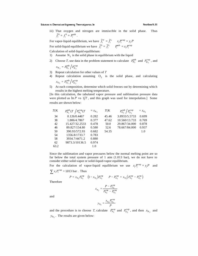
Solutions to Chemical and Engineering Thermodynamics, 3e Section 8.11
iii) That oxygen and nitrogen are immiscible in the solid phase. Thus
f f Pi i iS S sub= = .
For vapor-liquid equilibrium, we have f f x P y Pi i i i iV L vap= ⇒ =
For solid-liquid equilibrium we have f f P x Pi i i i iS L sub vap= ⇒ =
Calculation of solid-liquid equilibrium:1) Assume N2 is the solid phase in equilibrium with the liquid
2) Choose T, use data in the problem statement to calculate PHsub
2 and PH
vap2
, and
x P PN Nsub
Nvap
2 2 2=
3) Repeat calculation for other values of T4) Repeat calculation assuming O2 is the solid phase, and calculating
x P PO Osub
Ovap
2 2 2=
5) At each composition, determine which solid freezes out by determining whichresults in the highest melting temperature.
[In this calculation, the tabulated vapor pressure and sublimation pressure datawere plotted as ln P vs 1 T , and this graph was used for interpolation.] Some
results are shown below:
T K( ) P T P TNsub
Nvap
2 2( ) ( ) = xN 2
T K( ) P POsub
Ovap
2 2= xO2
34 0.126/0.4467 0.282 45.46 3.8933/5.5733 0.69938 1.806/4.7867 0.377 47.62 10.560/13.733 0.76942 15.427/32.2533 0.478 50.0 29.867/34.000 0.87846 89.827/154.80 0.580 52.6 78.667/84.000 0.93750 390.93/572.93 0.682 54.35 1.054 1356.8/1733.7 0.78358 3934.7/4471.2 0.88062 9873.3/10136.5 0.974
63.2 1.0
Since the sublimation and vapor pressures below the normal melting point are sofar below the total system pressure of 1 atm (1.013 bar), we do not have toconsider either solid-vapor or solid-liquid-vapor equilibrium.
For the calculation of vapor-liquid equilibrium we use x P y Pi i ivap = and
x Pi ivap bar∑ = 1013. . Thus
P x P x P P P x P P= + − ⇒ − = −N Nvap
N Ovap
Ovap
N Nvap
Ovap
2 2 2 2 2 2 2 21c h c h
Therefore
xP P
P PNOvap
Nvap
Ovap2
2
2 2
=−
−
and
yx P
PNN N
vap
22 2=
and the procedure is to choose T, calculate PNvap2
and POvap
2, and then xN 2
and
yN2. The results are given below:

Solutions to Chemical and Engineering Thermodynamics, 3e Section 8.11
T 75.5 77.5 80 82.5 85 87.5 90.1 KPN
vap2
1.013 1.333 1.849 2.467 3.284 4.200 bar
POvap
20.2187 0.3147 0.4267 0.5867 0.7600 1.013 bar
xN 21.0 0.713 0.455 0.288 0.158 0.074 0
yN21.0 0.938 0.830 0.700 0.512 0.305 0
Below is the vapor-liquid-solid phase diagram for O2 and N2 determined by experiment
(B.F. Dodge and A. K. Dunbar, J. Amer. Chem., Soc. 49, 501 (1927); B. F. Dodge, Chem. & Met.Eng. 35, 622 (1928); M. Ruhemann and B. Ruhemann, “Low Temperature Physics”, CambridgeUniv. Press, London, 1937, p. 100; and R.B. Scott, “Crogenic Engineering”, Van Nostrand,Princeton, 1959, p. 286). The main difference between this figure and our calculations is that O2
and N2 actually form mixed solids on freezing, which we presumed would not occur.
[I am grateful to my former colleague at the University of Delaware, Prof. K. Bischoff forbringing these data to our attention.]

Solutions to Chemical and Engineering Thermodynamics, 3e Section 8.11
8.11-12 Note: Error in Problem statement in 1st printing vapor pressure of isobutane is490.9 kPa not 4.909 kPa.Based on Illustration 8.4-2 this is a problem in vapor-liquid-liquid (3 phase)equilibrium. Also, from Problem 8.9-10, we have that the coexistence pressure isconstant over the whole range of average (or total) mole fractions for which twoliquid phases exist. From Illustration 8.4-2, one liquid phase is present forx xisobutane = ≤1 01128. and x1 09284≥ . . For overall mole fractions in the range
01128 0 92841. .≤ ≤x , two liquid phases exist. To compute the V-L-L coexistence
pressure in the one-liquid phase region, we use (neglecting fugacity coefficient
corrections) x P x P P1 1 1 2 2 2γ γvap vap+ = where P1 490 9vap kPa= . , and
P2 0493vap kPa= . , and γ1 and γ2 (or x1 1γ and x2 2γ ) are given in Table in
Illustration 8.4-2. Also, the van Laar constants are given there, so γ1 and γ2 can
be computed at other compositions. Results are given below
x1 x P1 1 1γ vap + x P2 2 2γ vap P
0 0 1 0493× . 0.493 kPa0.025 0 3068 490 9. .× + 0 9764 0 493. .× 151.10.05 05491 490 9. .× + 0 9555 0493. .× 270.00.075 0 7384 490 9. .× + 0 9371 0 493. .× 362.90.10 08843 490 9. .× + 0 9231 0 493. .× 434.6
0.1128 0 945 4909. .× + 0 914 0 493. .× 464.4↓ ↓ ↓ ↓
0.9284 464.40.95 0 9582 490 9. .× + 0 7325 0493. .× 470.70.975 0 9771 490 9. .× + 0 4318 0493. .× 479.9
1 490.9 490.9

Solutions to Chemical and Engineering Thermodynamics, 3e Section 8.11
8.11-13 The vapor pressure of water is 1.013 bar at 100°C. To compute the vaporpressure of acetone, we fit the data in the problem statement to
ln P A T Bvap = + and find A = −36189. , B = 109930. and
PACvap C100 3650 bar°( ) = . .
(a) To compute activity coefficients, we will use the van Laar model withα = 2 05. , β= 150. , as given in Table 7.5-1. Thus
ln.
.
. .
γα
α βγ
ACAC AC AC AC
AC AC
=+ −
=+ −
⇒ = =1 1
2 05
1 13667 1
1050 at 08
2 2x x x x
x
a fa f a fa f
and
ln.
.
. .
γβ
β αγ
WW W W W
W W at
=+ −
=+ −
⇒ = =1 1
150
1 07317 1
2 921 02
2 2x x x x
x
a fa f a fa f
At vapor-liquid equilibrium
x P x P PW W Wvap
AC AC ACvapγ γ+ =
Substituting the results for γ i , Pivap above yields
P = 3658. barThus, for all pressure above 3.658 bar only a liquid of composition xW = 02. ,
xAC = 08. will be present.
(b) This calculation is more difficult, since we can not calculate the dew point“pressure” (at fixed temperature) until the liquid phase composition andactivity coefficients are known. Thus the problem involves a trial-and-errorsolution of the equations
x P y PW W Wvap
Wγ = ; x P y PAC AC ACvap
ACγ = , and x xAC W+ = 1
where xW , xAC and P are the unknowns (The γ i can be calculated from the
xi using the van Laar equations). By repeated guesses, I find
P = 3601. bar; xW = 0295. and xAC = 0705.
Thus, for all pressures below 3.601 bar, only the vapor (of compositionyW = 020. , yAC = 080. ) is present.
Note: One should check the conditions of both parts (a) and (b) to the aboveproblem for the possible occurrence of two coexisting liquid phases.
8.11-14 Using the program VLMU with k nCO C2 6− = 011. (Table 7.4-1) results in no
solution at 140 bar and 75°C. However, trying the bubble point and dew pointpressure programs we obtain the following results (at T = 34815. K )

Solutions to Chemical and Engineering Thermodynamics, 3e Section 8.11
xCO2bubble point
P, baryCO 2
dew pointP, bar
yCO 2dew point
P, bar0.1 12.96 0.001 1.21 0.9 15.060.3 37.93 0.05 1.28 0.92 20.250.5 64.15 0.1 1.35 0.93 24.640.7 89.14 0.3 1.76 0.94 32.020.72 91.36 0.4 2.07 0.945 38.560.74 93.49 0.5 2.51 0.947 42.620.76 95.52 0.6 3.17 0.949 49.390.78 97.43 0.7 4.31 0.9495 52.750.80 99.17 0.73 4.83
0.75 5.25 Program doesn’tProgram doesn’t 0.78 6.03 converge at higher
converge at higher 0.80 6.70 CO2 concentrations
CO2 concentrations 0.82 7.56
Since the program doesn’t converge at higher concentrations of CO2 along either
the bubble point or dew point curves, we have to make an estimate of the CO2
concentration based on the data above. There are two possibilities: (1) The CO2

Solutions to Chemical and Engineering Thermodynamics, 3e Section 8.11
saturation of the liquid at 140 bar is in the retrograde region at somewhere betweenxCO2
of 0.8 and 0.95 [Note, simple equation of state programs, such as VLMU
typically do not converge in the retrograde region, and more sophisticatedalgorithms and numerical methods must be used]; (2) at 140 bar only the vaporexists, that is, all the hexane vaporizes.An alternative is to use the activity coefficient approach. We do this here usingregular solution theory and corresponding states for the fugacity coefficients. Thestarting point is the equilibrium condition
x f y fi i i i iγ L V=
which, for hexane translates to
xf
PP
V P P
RTy P
f
PH Hsat, H
Hvap H
LHvap
HH
γ FH IK−RS|T|
UV|W|= FH IKexp
c h
while for CO2 , which is considerable above its critical point, we have
xf P
PP
V P
RTy P
f
PCCCO CO
L
COCO
COL
COCO
2 2
2
22
22
bar barγ
=( )FHG
IKJ
−( )RS|T|UV|W|
= FH IK1013 1013.
exp.
,
Also, fitting vapor pressure data for n-hexane in “The Chemical EngineersHandbook” we find P TH
vap C= °( ) =75 1226 bar. . Also T = ° =75 34815C K.Next, we have
TC K( ) PC bar( ) δ cal cca f1 2 V L cc mola fn-hexane 507.4 29.69 7.3 ←Table 7.6-1→ 132CO2 304.2 73.76 6.0 ←Table 8.3-1→ 55
Tr Pr f Pa fsat f PCLc h f PVc h
n-hexane 0.686 4.715 0.732 ~0.08←Fig. 5.4-1CO2 1.144 1.898 ~1.15 0.65←Fig. 8.3-1
Thus
x y
x y
CO
3
3 CO CO
CO CO CO
2 2 2
2 2 2
m mol bar
348.15 K 8.314 10 bar m mol K
× × × × × −( )× × ( )
RS|T|UV|W|
= × ×
⇒ =
−
−115 737655 10 140 1013
0650 140
08238
6
5. . exp.
.
.
c h γ
γ
and
x y
x y
H H H
H H H
348.15 8.314 10
× × ×× × −( )
× ×RST
UVW = × ×
⇒ =
−
−0 732 1226132 10 140 1226
008 140
6628
6
5. . exp.
.
.
γ
γ

Solutions to Chemical and Engineering Thermodynamics, 3e Section 8.11
The ideal mixture γ i = 1a f solution is
yCO 2= 0 9696. xCO2
= 07988. (Easily solved using
yH = 00304. xH = 0 2012. Mathcad)
To obtain a more accurate solution, regular solution theory will now be used tocompute the γ i ’s
lnγφ δ δ
HHL
CO H CO2 2=−V
RT
2 2c hand
lnγφ δ δ
COCOL
H H CO
22 2=
−V
RT
2 2c h
using the ideal solution as a first guess and iterating, or using Mathcad and solvingdirectly, I obtain the following
yCO 2= 0 9620. xCO2
= 07747. Qualitatively in agreement
yH = 00380. xH = 0 2253. with the P-R e.o.s. results.
Note the enormous solubility of carbon dioxide in hexane and, indeed, in reservoircrude! That is why carbon dioxide has been used in enhanced oil recovery (crudeoil swells so more is recovered, and viscosity drops so the trapped oil in the earthmatrix flows more easily.)
8.11-15 Possibilities: 1 liquid phase1 vapor phase2 phases vapor + liquid2 phases liquid + liquid3 phases liquid + liquid + vapor
We will assume that only one liquid phase exists and show that this assumption iscorrect.From the data in the problem statement
PEACvap bar= 09475. and PEOH
vap = 08879. bar
The bubble point pressure of an equimolar mixture is
P x Pi i i= = × +( ) =∑ γ vap 05 0896 05 09475 08879 1148 bar2. exp . . . . .c hSince the applied pressure is 1.8 bar, no vapor is in equilibrium with an equimolarmixture at the specified temperature of 75°C. Now we have to check to seewhether one or two liquids are present at equilibrium. To determine this we startwith
RT AxA
RTx A xi j i j jln lnγ γ= ⇒ − = ′2 2 2
with ′ =A 0896. given in the problem statement. Therefore A A RT RT= ′ = 0896. .Now from eqn. 8.4-14 we have that the upper consolute temperature (the highesttemperature at which two liquids exist) for the one-constant Margules equation is

Solutions to Chemical and Engineering Thermodynamics, 3e Section 8.11
TA
R
RT
RTUC K= = = =
2
0896
20448 155 97
.. .
This temperature is so much below the system temperature of 348.15 K, that thesingle liquid phase is the stable phase. Therefore, the equimolar mixture at 75°Cand 1.8 bar is stable, and the only phase present.
8.11-16 For an azeotropic mixture, from eqn. (8.1-3)γ
γ
γ
i ivapP P
x
x
=
= = =
= = =
/
..
..
..
..
C C
B C
0510 2747
024611167
0510 2747
024411258
a fa f
Since the two activity coefficients are so close, and the azeotrope occurs near0.5 mole fraction, so I will use the one-constant Margules equation.
G x
RTx x
Ax x A
exC
C C B B
C B
== + = + =
= = ( )( ) =
051051 11167) 0 49 11258 011435
051 0 49 011435
.ln ln . ln( . . ln( . ) .
. . .
a f γ γ
A = 0.4576 therefore Gex =8.314×(273.15+40) ×0.4576 = 1191xCxB
RT x x
RT x x
P x x x x x
y xx x
P x
ln exp .
ln exp .
exp . . ( ) exp . .
( )exp . .
γ γ
γ γC B C B
B C B C
C C C B C
C CC C
C
or
or
Also
= =
= =
= − + −
=−
1191 0 4576
1191 0 4576
0 4576 1 0246 1 04576 0244
04576 1 0246
2 2
2 2
2 2
2
b gb g
a f a fc h b g
a fc ha f
b) The LLE upper consolute temperature is
TA
RUC K
which is much below the freezing point of each compound.
= =× ×
×=
2
0 4576 31315 8314
2 83147165
. . .
..
yi
xi
0 0.5 10
0.5
1
Pi
Pi
xi
yi
,0 0.5 1
0.24
0.26
0.28

Solutions to Chemical and Engineering Thermodynamics, 3e Section 8.11
c) Freezing point depression
ln
ln
ln
,
,
, ,
,
,
,
xH T
R T T
T T
R
H Tx
TT
RT
H Tx
fusm
m
mfus
m
m
mfus
m
S Ssolvent
solvent
solvent solventS S
solvent
solvent
solventS S
or
or
γ
γ
γ
a f b g
b g a f
b g a f
= − −FHG
IKJ
= −
=−
∆
∆
∆
1 1
1 1
1
For cyclohexane freezing
For benzene freezing
B BB B
C CC C
Tx x
Tx x
= +
− × + =−
=+
− × + =−
27315 66
18314 27315 66
2630
279 751 08844
27315 553
18314 27315 553
9953
278 68
1 02378
. .. ( . . )
ln
.. ln
. .. ( . . )
ln
.
. ln
γ γ
γ γ
a f a f
a f a f
8.11-17
a)
jC D
RTRT x CD x
x D x D x x Dx x
D Dx
11
1 1 1
1 1 1 1 11
1
1
1
1
1
1
= − ∇ + = ∇
∇ + ∇ = ∇ = + ∂∂
LNM
OQP
= + ∂∂
LNM
OQP
o o
o o
o
µ γ
γ γ
γ
ln
ln lnln
ln
ln
c h
b)
RT A x
xx
xx
xx
ART
x
xAx x
ln ( )
ln
ln
ln ln
γ
γ γ γ
1 12
1
11
1
11
1
21
22
21 2
1
2
= −
∂∂
= ∂∂
= − ∂∂
= −∂FH IK
∂= −
D Dx
DA
RTx x= +
∂∂
LNM
OQP = −FH IKo o1 1
21
11 2
ln
ln
γ
c) 1) Infinite dilution x D D1 0 and → → o
Tci
Tbk
xi
xk
,0 0.5 1
0
200
400

Solutions to Chemical and Engineering Thermodynamics, 3e Section 8.11
2) At LLE critical point at UCTA
Rx x= = =
2051 2 .
D DR T
R T= −
× × ××
LNM
OQP =o
UC
UC
12 2
0
3) Negative deviations from Raoult’s law ⇒ A is negative
D DA
RTx x A D D= −FH IKo o with negative, > 1
21 2
8.11-18 (also available as a Mathcad worksheet).
8.11-18
γ Pinf 16 γ Hinf 6.34 PvapP 20.277 PvapH 28.022
Using the van Laar equation
α ln γ Pinf( ) β ln γ Hinf( )
i 1 2, 99.. xi
0.01 i.
γ Pi
expα
1α
β
xi
1 xi
2γ H
iexp
β
1β
α
1 xi
xi
2 Pi
xi
PvapP. γ Pi
. 1 xi
PvapH. γ Hi
.
Pi
xi
0 0.5 120
30
40
50
yPi
xi
PvapP. γ Pi
.
Pi
0.920522
0.097206
yPi
0.990.01 xi
0 0.5 10
0.5
1

Solutions to Chemical and Engineering Thermodynamics, 3e Section 8.11
So this system exhibits either azeotropy or LLE. Test for LLE
x11 0.01 x12 0.90
Given
x11 expα
1α
β
x11
1 x11
2. x12 exp
α
1α
β
x12
1 x12
2.
1 x11( ) expβ
1β
α
1 x11
x11
2. 1 x12( ) exp
β
1β
α
1 x12
x12
2.
y find x11 x12,( )
x11 y0
x11 0.113= x21 1 x11 x21 0.887=
x12 y1
x12 0.684= x22 1 x12 x22 0.316=
x12 0.684=
So there is LLE

9
Note that many of the problems in this chapter can be solved relatively easily with twoprograms. The first is CHEMEQ which makes the calculation of the chemical equilibriumconstant at any temperature very easy. The second is an equation solving program, suchas Mathcad, for solving the nonlinear algebraic equation(s) which result. It is advisablethat students know how to use both. [I have used Mathcad for many of the problemsolutions reported here.]
9.1 From Equation 9.1-18
ln. .
ln . .
K TG
RT
K K T
a
a a
= °( ) =− ° °( )
= −×
⇒ = − = °( ) = × −
2525 17,740
8 314 29815
71566 and 25 77967 10 4
CC
C
rxn∆
Next using Eqn. 9.1-23b with ∆a = 16736 . J mol K ; ∆ ∆ ∆ ∆b c d e= = = = 0 gives
[Note: Error in problem statement of first printing. ∆CP J mol K= 16736 . not
kJ/mol K]
ln.
ln.
. . .
.
.ln
.
., . .
.. . .
K T
K T
a
R
RH a
a
a
=( )=( )
=
+ − ( ) + × −
=
+ − + × −FH IK= + =
− −
500 K
298 15
500
298 15
1298 15 298 15 500 298 15
16736
8 314
500
298 151
831455 480 16736 298 15
1
500
1
298 1510407 82228 92635
1 1
K
rxno
∆
∆ ∆
ln ln . . . . .
.
K T K T
K Ta a
a
=( ) = =( ) + = − + =⇒ =( ) =
500 K 298 15 9 2635 71566 92635 2107
500 K 8 225

Solutions to Chemical and Engineering Thermodynamics, 3e Chapter 9
Mass Balance TableSpecies In Out yi y Xi =( )09436.
IPOH 1 1− X 1 1−( ) +( )X X 0.0290
Prop 0 X X X1+( ) 0.4855
H2 0 X X X1+( ) 0.4855
Total 1+ X → calculated after X wasfound below
Now Ka a
a
X P
X X
X
Xa = = =+( ) −( )
=−
H Prop
IPOH
2 bar 1 bar2 2
2
1013
1 1 1
.a fb g .
X K Xa2 21= −( ) ; 1 2+ =K X Ka aa f or X K Ka a= +1a f ;
K Xa = ⇒ = ⇒8 225 09436 9436%. . . of alcohol is converted.
9.2 Reaction: CaC O CaCO CO2 4 3= +
Ka a
aa Pa = = =CaCO CO
CoC OCO CO
3
2 4
T °( )C 375 388 403 410 416 418
P Pdiss CO kPa= ( ) 1.09 4.00 17.86 33.33 78.25 91.18
K Pa = CO 100 0.0109 0.0400 0.1786 0.3333 0.7825 0.9181
ln Ka –4.5282 –32.315 –1.7356 –1.1112 –0.2581 –0.1052
T K( ) 648.15 661.15 676.15 683.15 689.15 691.15
− = °RT K Galn ∆ rxn
2 4kJ / mol CaC O
reacted
24.401 17.763 9.757 6.3113 1.4788 0.6351
Now d G RT
d T
d K
d T
H
RTa∆ ∆rxn
orxnob g
= − = −ln
2 (1)
and ∆∆ ∆
SH G
Trxno rxn
orxno
=−
(2)
Plot the data for ln Ka vs. T. It falls on a reasonably straight line of slope ~ 0.106.
i.e., d K
dTaln
~ .0103 . Thus, ∆H RTrxno ≅ 0103 2. , which follows from Eqn. (1). Once
∆Hrxno is evaluated, Eqn. (2) can be used to get ∆Srxn
o . The results are given
below:

Solutions to Chemical and Engineering Thermodynamics, 3e Chapter 9
T °( )C 375°C 403°C 418°C
∆Hrxno 358.7 390.4 409.9 kJ/mol CaC O2 4 reacted
∆Srxno 0.5159 0.5630 0.5984 kJ/mol K CaC O2 4 reacted
9.3 Reactions: C CO+ ( ) = ( )2 2COg g (1)
2CO Og g( ) = + ( )2C 2 (2)
Mole balance tableSpecies Initial Final yi
C —CO2 1 1 1− X 1 11 1 2− + −X X Xa f a fCO 0 2 21 2X X− 2 11 2 1 2X X X X− + −a f a fO2 0 X2 X X X2 1 21+ −a f
1 1 2+ −X X
ay P
yii
i= =1 bar
since P = 1 bar
(a) From the program CHEMEQ we find that K Ta,1 2000 K 39050=( ) =
at T K K X Ka a a= = × ⇒ =−2000 K 2 445 10 0 0 and 39050219
2 2 1, , ,. ~ , ~
Ka
a aX X
X X XX
X XX
K
Kaa
a,
,
,1
1 22
1 1 2
12
1 112 1
1
41 1
41 1 4
1= = −− + −
≅− +
⇒ =+
=CO2
C CO 2
a fa fa f
a fa fa f
(as one would expect with such a large equilibrium constant)(b) At 1000 K using CHEMEQ
640 650 660 670 680 690 7006
4
2
0
Temperature (K)
ln K
a

Solutions to Chemical and Engineering Thermodynamics, 3e Chapter 9
K T
K T
a
a
,
,
.
.
1
223
1000 K 1835
1000 K 3984 10
=( ) =
=( ) = × −
X11835
4 18350561=
+=
.
..
Thus, the composition of the gas leaving the graphite bed is
Species 2000 K 1000 KCO2 2 594 10 5. × − 0.283
CO 1.0 0.717O2 0 0
9.4
KG
RT
a
aa
f T P
f T P
V
RTP
a
ii
i
i
= −RST
UVW =−
×RST
UVW =
= =( )
=( )= −( )RST
UVWA
exp exp. .
.
;,
,exp
∆ rxno
diamond
graphitePoynting correction
terms assumedincompressible solid
where bar
bar
2866
8 314 298 1503147
11
a
a
V P RT
V P RT
V V P
RTdiamond
graphite
dim
gr
dim gr bar
bar
bar=
−( )−( )
=− −( )RS|T|
UV|W|exp
expexp
1
1
1k pn s
d i
where
V
V
P
RT
G
RT R
P
diam3
graph3
rxno
g mol
g cccc mol m mol
g mol
.25 g cc cc mol m mol
cc - bar J mol
barJ mol
cc molJ cc
= = = ×
= = = ×
= −( ) −( ) =−
= −
⇒ − = = =
−
−
12
35134188 34188 10
12
253333 53333 10
0 314734188 53333 1 2866
12866
1914514970 14970 bar
6
6
.. .
. .
ln .. .
..
∆
or P = 14971 bar .
Thus for P < 14971 bar ; a
aKa
diam
graph
> and graphite is stable phase
for P > 14971 bar ; a
aKa
diam
graph
< and diamond is stable phase
⇒ Need a hydraulic press capable of exerting 14971 bar to convert pencil leads todiamonds. (Also, should consider a higher temperature!)
9.5 For convenience, write reaction as N O 2NO2 2 2+ =Species balance table

Solutions to Chemical and Engineering Thermodynamics, 3e Chapter 9
Species Initial Final yi
O2 1 1− X 1 4762−( )X .
N2 0 79 021 3762. . .= 3762. − X 3762 4 762. .−( )X
NO 0 2 X 2 4 762X .
4.762
Since P = 1013. bar ; ay P
ii=
1 bar
Ky
y y
X
X X
XK
K
a
a
a
= =( )
−( ) −( )
=− + +
−
NO2
N O2 2
which has the solution2
1 3762
2 381 19073 15048
4 1
2
.
. . .
a fUsing the program CHEMEQ and its data base the following results are obtained(which agree with Figure 9.1-2)
T °( )C 1500 1600 1800 2000
Ka 0 9795 10 4. × − 01924 10 3. × − 05861 10 3. × − 01455 10 2. × −
X 0.00954 0.0133 0.0231 0.0361
T °( )C 2100 2200 2400 2500
Ka 0 2154 10 2. × − 0 3077 10 2. × − 05718 10 2. × − 0.007487
X 0.0438 0.0520 0.0701 0.0796
T °( )C 2600 2800 2900 3000
Ka 0.009539 0 01450. 0.01732 0.02028
X 0.0893 0.1086 0.118 0.1269
9.6 (a) From Appendix IV
∆H fo ∆G f
o
Na SO 10H O2 4 2⋅ –4322.5 –3642.3 kJ/mol
Na SO2 4 –1382.8 –1265.2
H O2 –241.8 –228.6
⇒ = °( ) = −( ) − −( ) − −( ) = −= °( ) = −
⇒ = °( ) = +×( )
= +
= °( ) = ×
∆∆
H T
G T
K T
K T
rxn
rxn
a
a
C kJ mol
C kJ mol
C
C
25 43225 13828 10 228 6 521 7
25 911
2591100
8 314 2981536751
25 9139 1015
. . . .
.
ln,
. ..
.
Now

Solutions to Chemical and Engineering Thermodynamics, 3e Chapter 9
Ka
a a P
P
aNa SO 10H O
Na SO H O10
H O
H O
2 4 2
2 4 2 2
2
bar
C bar bar
=⋅
=FHG
IKJ = ×
⇒ °( ) = × =
⋅
−
109139 10
25 2503 10 00253
10
15
2
.
. .
(b) At 15°C. Since 15°C is near 25°C we will correct Ka for temperature using only
the ∆Hrxno term, i.e.
ln. .
.
exp . .
. .
K T
K T
H
R
K T K T
P
a
a
rxno
a a
H O
C
C
C C
C bar bar2
= °( )= °( )
= − −FH IK =
= °( ) = = °( ) ( ) = ×
°( ) = × =−
15
25
1
288 15
1
2981573438
15 25 7304 1358 10
15 1221 10 0 01221
19
2
∆
Experimental data (Baxter and Lansing, J.A.C.S. 42, 419 (1920))P
P
P
H O
H O
H O
2
2
2
C bar
C
C
0 0003693
15 001228 bar
25 00256 bar
°( ) =
°( ) =
°( ) =
.
.
.
9.7 (also available as a Mathcad worksheet)
Ka
a a
y
yaCS
C S
CS
S
2
2
2
2
= = . Since aC = 1 (solid), and P = =1 bar standard state
pressure.Species balance table:
Species Initial Final yi K X Xa = −( )1
C — — —S2 1 1− X 1−( )X ⇒ or
CS2 0 X X X K K= +a a( )1
1
Using CHEMEQ I find Ka C750 8478°( ) = . and Ka C1000 6 607°( ) = . . Therefore
X 750 0894°( ) =C . and X 1000 0869°( ) =C . . X y= CS2 is the percentage
equilibrium conversion of sulfur.
9.8 (a) Ba NO3a f2 solution
I z C C C C C
C C C C
= = ( ) + ( ) + ( ) + ( )
= + + +
∑1
2
1
22 1 1 1
1
24
2 2 2 2 2i i Ba NO Ag Cl
Ba NO Ag Cl
3
3
m rm r
but C C CAg Cl AgCl= = ; C CBa Ba NO3= a f2
; C CNO Ba NO3 3= 2 2a f

Solutions to Chemical and Engineering Thermodynamics, 3e Chapter 9
I C C C C C= + + = +1
24 2 2 3
2 2 2Ba NO Ba NO AgCl Ba NO AgCl3 3 3a f a f a fn s
CBa NO3a f2 CAgCl I I ln Ks , where
K Cs = AgCl2
2111 10 4. × − 01309 10 4. × − 6 4639 10 4. × − 2 542 10 2. × − –22.4873
7 064 10 4. × − 01339 10 4. × − 213259 10 4. × − 4 618 10 2. × − –22.4420
44 02 10 4. × − 01450 10 4. × − 132 21 10 4. × − 11498 10 2. × − –22.2827
560 10 4. × − 01467 10 4. × − 168147 10 4. × − 12 967 10 2. × − –22.2594(mol/liter) (mol/liter)
(b) La NO3a f2 solution
Using similar analysis to that above yields I C C= +63La NO AgCl3a f .
CLa NO3a f2CAgCl I I ln Ks , where
K Cs = AgCl2
1438 10 4. × − 01317 10 4. × − 87597 10 4. × − 2 9597 10 2. × − –22.4751
5780 10 4. × − 01367 10 4. × − 348167 10 4. × − 59006 10 2. × − –22.4006
166 10 4. × − 01432 10 4. × − 99 7432 10 4. × − 9 9872 10 2. × − –22.3077
2807 10 4. × − 01477 10 4. × − 168 568 10 4. × − 12 983 10 2. × − –22.2458(mol/liter) (mol/liter)
I mol / liter( ) 12
Except for the single point or high ionic strength (AgCl in KNO3 ), all the data
fall on a straight line.

Solutions to Chemical and Engineering Thermodynamics, 3e Chapter 9
9.9 For BaSO Ba SO4 4= +++ −− , we have
I z M C C C Si i= ≅ + = =∑ ++ −−
1
2
1
22 2 4 42 2 2
Ba SO BaSO4 4o t
where S = solubility of BaSO4 in moles/liter
also K C C Ss = =+ + −−Ba SO4
2 . Note we have neglected the difference between M
and C. Thus
T °( )C α Table 7.6( ) S K Ss = 2 I S= 2
5 1.140 156 10 6. × − 2 43 10 10. × − 7 9 10 3. × −
10 1..149 16.7 2.789 8.17315 1.158 18.3 3.349 8.55620 1.167 19.8 3.920 8.90025 1.178 21.6 4.666 9.295
(mol/liter) mol litera f2 mol litera f1 2
Now KK
s =( ) + −
+ −
+
±+
a molal1 ν ν
ν νγ and K
Ks
s= °
±++ −γν ν . K Ks°= ( ) + −+
a molal1 ν ν or
KKs
a molal
= °( ) + −+1 ν ν and
ln ln ln
ln
ln ln
K K
K z z I
K I K I
s s
s
s s
= °−
= °+ +
= °+ ⋅ ×( ) = °+
±++ −
++ −− ++ −−
ν ν
ν ν α
α α
Ba SO Ba SO4 4e j2 2 2 16
or K K S S Ss s° = − = −exp exp16 162α αd i d i .
Note that Ka is the equilibrium constant for the reaction
BaSO Ba ideal 1 molal SO ideal 1 molal4 s aq aq( ) = +++ −−, ,a f a f4
and ∆G
TR Krxn
a= − ln . Thus we have
T °( )C Ks° ln Ks°∆G
TR Ka
rxn = − ln ∆Hrxn ∆Grxn ∆Srxn
5 2 261 10 10. × − –22.2100 184.654 20490 51,362 –110.99
10 2.587 –22.0754 183.535 21234 51,968 –108.5415 3.094 –21.8964 182.047 21991 52,457 –105.7320 3.607 –21.7430 180.771 22760 52,993 –103.1325 4.275 –21.5731 179.359 23543 53,476 –100.40
mol lita f2 J
mol KFH IK
(J/mol) (J/mol) (J/mol)

Solutions to Chemical and Engineering Thermodynamics, 3e Chapter 9
∆G Trxn is essentially a linear function of T as can be seen by plotting the data.
Also, from the plot we have
∂∂
∆ ∆ ∆∆
G T
T
G T
Trxn rxn 2 J mol K
a f a f~ ~ .−026485
However∂
∂∂
∂G T
T
H
TH T
G T
TT
a f a f= − ⇒ = − = ( )
22 2 026485∆
∆rxn
rxn .
Finally
∆∆ ∆
∆∆ ∆
SH G
TS
H G
T=
−⇒ =
−rxn
rxn rxn
Both ∆Hrxn and ∆Srxn are given in the table on previous page.
9.10 (also available as a Mathcad worksheet)(a) Using the program CHEMEQ, the following results are obtained
rxn 1 C H 3H O 3CO 7H
rxn 2 C H 6H O 3CO 10H3 8 2 2
3 8 2 2 2
+ = ++ = +
rxn Ka
1000 K
Ka
1100 K∆Hrxn
o
1000 K
∆Grxno
1000 K
∆Hrxno
1100 K
∆Grxno
1100 K1 01343 1012. × 0 4806 1014. × 537.260 –213.030 538.140 –288.11
2 0 3332 1012. × 0 3851 1014. × 432.380 –220.590 436.440 –286.09
All energies in kJ/mol of C3H8
(b) Ka a
a aa,1
7
= H CO3
C H H O3
2
3 8 2
and Ka a
a aa,2
10
= H CO3
C H H O6
2 2
3 8 2
where, since P = 1 bar
ay P
yii
i= =1 bar
.
Species balance table
Species In Out yi
C H3 8 1 1 1 2− −X X 1 1 2− + ∑X Xa fH O2 10 10 3 61 2− −X X 10 3 61 2− − ∑X Xa fCO 0 3 1X 3 1X ∑
CO2 0 3 2X 3 2X ∑H2 0 7 101 2X X+ 7 101 2X X+ ∑a f
∑ = + +11 6 1 2X Xa fThus
KX X X
X X X X X Xa,1
13
1 27
1 2 1 23
1 26
27 7 10
1 10 3 6 11 6 6= +
− − − − + +a f
a fa f a f

Solutions to Chemical and Engineering Thermodynamics, 3e Chapter 9
KX X X
X X X X X Xa,2
23
1 210
1 2 1 26
1 26
27 7 10
1 10 3 6 11 6 6= +
− − − − + +a f
a fa f a fAlso
K
K
X X X
X X Xa
a
,
,
1
2
13
1 23
23
1 23
10 3 6
7 10= − −
+a fa f
In view of the very large numerical values of the equilibrium constants, weexpect X X1 2 1+ ~ . Using this approximation we get
KX X
X X Xa,1
13
27
1 2 23 6
27 7 3
1 7 3 17= +
− − − ( )a f
a fa f ; KX X
X X Xa,2
23
210
1 2 26 6
27 7 3
1 7 3 17= +
− − − ( )a f
a fa fand
K
K
X X
X X
K
K
X X
X X
X X
X Xa
a
a
a
,
,
,
,
1
2
13
23
23
23
1
2
1 3
1 2
2 2
2 2
2 2
7 3
7 3
7 3
7 3
1 7 3
7 3= −
+⇒
FHG
IKJ = −
+= − −
+a fa f
a fa f
a fa fa f
Note that this last equation is a simple quadratic equation for X2 given Ka,1
and Ka ,2 . Also, then X X1 21= − .
(c) at 1000 K: X1 0527= . ; X2 0473= .
at 1100 K: X1 0 603= . ; X2 0397= .
Thus we obtain
Species yi 1000 K( ) yi 1100 K( )C H3 8 0 0
H O2 0.328 0.342
CO 0.093 0.106CO2 0.083 0.070
H2 0.495 0.482
9.11 (also available as a Mathcad worksheet)
Reaction: SO1
2O SO2 2 3+ =

Solutions to Chemical and Engineering Thermodynamics, 3e Chapter 9
Species balance table
Species Initial Final yi
SO2 1 1− X 1
338 05
−−
X
X. .
O21
2
1
21−( )X
1 2 1
338 05
−( )−
X
X. .
N21
2
079
021188× =
.
.. 1.88
188
338 05
.
. .− X
SO3 0 XX
X338 05. .−
3381
2. − X
Since P = 1013. bar ; ay P
yii
i= =1
1013 bar
.
Ka
a a
y
y y
X X
Xa
SO
SO O
SO
SO O
3
2 2
3
2 2
= = =−( )
−( ) ( )1 2 1 2
1 2
1 2 3 2 1 2
338 05
1013 1 05
. .
. .
The chemical equilibrium constant for this problem was calculated using theprogram CHEMEQ and then the problem was solved using Mathcad. The resultsappear belowT °( )C Ka X ySO2
yO2ySO3
0 1016 1014. × ~1 ~0 ~0 0.3472
100 08625 109. × ~1 ~0 ~0 0.3472
200 01012 107. × 0.9998 6148 10 5. × − 3074 10 5. × − 0.3472
300 01265 105. × 0.9967 0.001139 0.000569 0.3459
400 05903 103. × 0.9750 0.008635 0.0004317 0.3371
500 0 6188 102. × 0.8935 0.0363 0.0182 0.3046
600 01104 102. × 0.7090 0.0962 0.0481 0.2343
700 0 2847 101. × 0.4569 0.1723 0.0862 0.1450
800 0.9566 0.2467 0.2313 0.1157 0.0757900 0.3951 0.1252 0.2637 0.1319 0.03771000 0.1863 0.0655 0.2792 0.1396 0.01961100 0.09969 0.0366 0.2866 0.1433 0.01091200 0.05862 0.0220 0.2903 0.1451 0.006521300 0.03722 0.0141 0.2923 0.1462 0.004181400 0.02518 0.0096 0.2934 0.1467 0.00285

Solutions to Chemical and Engineering Thermodynamics, 3e Chapter 9
9.12 Reaction: C H Cl C H Cl2 4 2 2 4 2+ =However, C H Cl2 4 2 is a liquid at 50°C — 2 phase reaction!
Some physical property data
Species Normal boiling point Pvap C50°( ) TC PC bar
C H Cl2 4 2 83.47°C 0.288 bar
C H2 4 –88.63°C 122.5 bar‡ 9.2°C 50.36
Cl2 –34.6°C 14.87 bar
‡Since ethylene is above its critical temperature, its “liquid-phase” vapor-pressurewill have to be estimated if we are to do the vapor-liquid equilibrium calculation.However, since we need only a moderate extrapolation (from T = °9 2. C toT = °50 C ), we will do an extrapolation of the vapor-pressure data, and not useShair’s correlation. Using vapor-pressure equation in the Handbook of Chemistry
and Physics, we find Pvap C50 1225°( ) ~ . bar for ethylene.
Note: To be consistent, all vapor pressure data for this problem have been takenfrom the Handbook of Chemistry and Physics. The data differs, in many cases by±20% from The Chemical Engineers’ Handbook . I believe the latter may be moreaccurate.Species balance table
Species Initial FinalC H2 4 1 1− X = +y V x LC H C H2 4 2 4
Cl2 1 1− X = +y V x LCl Cl2 2
C H Cl2 4 2 0 X = +y V x LC H Cl C H Cl2 4 2 2 4 2
Also, since P = 1 bar , ay P
yii
i= =1 bar
for species whose standard state is a vapor.
Note: An obvious first guess is that no C H Cl2 4 2 is present in the vapor phase,
and no Cl2 or C H2 4 is present in the liquid phase. Since the standard states of
1
0
Xi
YSO2i
YO2i
YSO3i
1.4 103.0 T
i
0 500 1000 15000
0.5
1

Solutions to Chemical and Engineering Thermodynamics, 3e Chapter 9
C H2 4 and Cl2 are as pure vapors and C H Cl2 4 2 is as a liquid, this would result in
an equilibrium relation of the form
Ka
a aaC H Cl
C H Cl
2 4 2
2 4 2
= =⋅
=1
1 2 1 24
which clearly can not be true! Therefore, to obtain the correct solution to thisproblem we must consider the possibility that all species may be present in allphases!In the table above, L and V are the total number of moles in the liquid and vaporphases, respectively. L V+ = 1Phase equilibrium: f f y P x PV
iL
i i i i1 = ⇒ = γ vap
Chemical equilibrium: (standard state: C H2 4 and Cl2 = vapor; C H Cl2 4 2 = pure
liquid)
Kx
y yaC H Cl C H Cl
C H Cl
2 4 2 2 4 2
2 4 2
=γ
Now using data in Appendices II and IV, and Eqn. 9.1-23b we obtain
K Ta C= °( ) ×50 11 1023~ . a huge number.
⇒ × × =y y xC H Cl Cl C H Cl C H Cl2 4 2 2 2 4 2 2 4 2c h 11 1023. γ
⇒ Reaction goes, essentially, to completion.Vapor-liquid equations
y x y x y xC H Cl C H Cl C H Cl C H C H C H Cl Cl Cl2 4 2 2 4 2 2 4 2 2 4 2 4 2 4 2 2 2 = ( ) = ( ) = ( )γ γ γ0 284 121 14 68. ; ; .
Now going back to chemical equilibrium relation
x x xC H C H Cl Cl C H Cl C H Cl2 4 2 4 2 2 2 4 2 2 4 2γ γ γc hc h c h× ( )( ) × =14 68 121 11 1023. .
Since, for this system, we expect all the activity coefficients to be of reasonable size(less than, say, 10), it is clear that the only solution is xC H Cl2 4 2
~ 1 ,
x xC H Cl2 4 2= = 0 [actually, these latter mole fractions will be of the order 10 13− ]
Plugging these values back into the vapor-liquid equilibrium equation, we findyi <∑ 1 . ⇒ No vapor phase!
Thus, the solution to this problem is that there is no vapor phase present atequilibrium, only a liquid phase. The reaction goes to completion in the liquidphase, so that
xC H Cl2 4 2= 1 , xC H2 4
= 0 , xCl2= 0 .
9.13 G G RT x G RT xi i i i i i i= + = + ÷ ÷ln lnγ γ where
xi = apparent mole fraction = °°∑
N
Ni
j
xi÷ = actual mole fraction =
∑N
Ni
j
In the model, γ i÷ = 1 , since the ternary mixture is ideal.
⇒ = =+ +
× + °°
=°
× + °+ +
÷
γ ii
i
i
A B B
A B
i
i
i
A B
A B B
x
x
N
N N N
N N
N
N
N
N N
N N N2 2

Solutions to Chemical and Engineering Thermodynamics, 3e Chapter 9
⇒ = + °+ +
γ AA B
A B B
N NN N N
2
and γ BB
B
A B
A B B
NN
N NN N N
=°
= + °+ +
2
Now consider the chemical equilibrium:
InitialNumber moles
Finalnumber moles
Mole fractionxi
A NA NAN
N N NA
A B B+ −°2
B NB° N XB
° −2 N N
N N N
B B
A B B
°
°
−
+ −
22
2
B2 — XN
N N NB
A B B
2
2+ −°
N N X
N N N
A B
A B B
+ −
= + −
°
°2
Ka
a
N N N N
N N
B
B
B A B B
B B
a = =+ −
−
°
°2 2 2
2
2 22
c hc h
Solving this equation gives
NN N k N N k K N k
BB A B A A B
2
2 24
2=
+ − + −° ° °c h c h c hwhere k K= +4 1a , and
22
2 2 2
2 2 2 1 2kN
N Nx kx kx kx x x
kx kx k
B
A Ba B B a B a
a B
+= + − + +
= + − = −
° c hδ δ
and δ = −( ) + + + +2 1 22 2 1 2k x kx kx kx x xa B B a B ac h
Also we obtain
NN N
kkB
A B
2 22=
+−
°c hδ ; N N
N N
kkB B
A B= −+
−°°c h
2 δ
N N N N NkA B B A B+ + = + ° FH IK2 2
a f δ and
N NN N N
kA B
A B B
+ °+ +
=2
2δ
Thus
γδA
A B
A B B
N NN N N
k= ++ +
=°
2
2 and
γ
δδ δ
BB A B
B A B B
B BA A B B A
N N N
N N N N
k
x k
k
xx kx x kx x
=+
+ +
= − −( )LNM
OQP = + + −
°
°
c hc h
c h 2
12 2 2
22 2 1 2

Solutions to Chemical and Engineering Thermodynamics, 3e Chapter 9
9.14 (also available as a Mathcad worksheet)
Reactions: C H OH1
2O CH CHO H O2 5 2 3 2+ = + rxn 1
C H OH CH CHO H2 5 3 2= + rxn 2
Species balance table:
Species In OutC H OH2 5 1 1 1 2− −X X
O2 0.75 0 75 05 1. .− X
N2079
0 21075 28214
.
.. .× = 2.8214
H O2 0 X1
CH CHO3 0 X X1 2+H2 0 X2
Σ4 571
1
2 1 2. + +X X
Using the program CHEMEQ we obtain
Ka, .1137 228 10= × aerobic reaction
Ka, .2 6 643= is greatly favored!
With these values of the equilibrium constant we obtain X1 1~ and X2 0≅ [all ethyl alcohol used
up in first reaction]. Therefore, yC H OH3 5~ 0, yO2
~ .0 049, yN2~ .0556, yH O2
~ .0197,
yCH CHO3~ .0197 and yH 2
~ 0.
9.15 (also available as a Mathcad worksheet)C H C H H3 8 3 6 2= + rxn 1
C H C H CH3 8 2 4 4= + rxn 2Species balance table
Species Initial Final yi
C H3 8 1 1 1 2− −X X 1
11 2
1 2
− −+ +
X X
X X
C H3 6 0 X1X
X X1
1 21+ +
H2 0 X1
X
X X1
1 21+ +
C H2 4 0 X2X
X X2
1 21+ +
CH4 0 X2X
X X2
1 21+ +Σ 1 1 2+ +X X
In general, we have ay P
ii=
1 bar, thus

Solutions to Chemical and Engineering Thermodynamics, 3e Chapter 9
Ka a
a
y y
y
P P X
X X X Xa,112
1 2 1 21 1 1 1= = F
HIK =
− − + +C H H
C H
C H H
C H
3 6 2
3 8
3 6 2
3 8 bar bara fa f
Similarly
Ka a
a
P X
X X X Xa,222
1 2 1 21 1 1= =
− − + +C H CH
C H
2 4 4
3 8 bar a fa f
Also K
K
X
Xa
a
,
,
2
1
22
12= , so define α = =X
X
K
Ka
a
2
1
2
1
,
,
. Thus
KP X
X X
P X
Xa,1
12
1 1
12
212
1
1 1 1 1
1
1 1=
− +( ) + +( )=
− +( ) bar bara f
a fa fa f
α α α
(a) Constant pressure case: P 1 bar= 1
⇒ =+ +
XK
K K
a
a a
11
11 2
21 2 2
1
,
, ,d i and X
K
K K
a
a a
22
11 2
21 2 2
1=
+ +
,
, ,d iResults are given in table below.
(b) Constant volume case: Assume gas is ideal
PV NRT PN
N
T
TX X
Tf
f
i
f
i
= ⇒ = = + +LNM
OQP1
298 151 2a f.
bar
or
PX T
KX T X
X X
X T
X
XT
K K KT
K K
XT
K K KT
K K
f
a
a a a a a
a a a a a
= + +( )
⇒ =+ +( )+ +( ) − +( )
=− +( )
⇒ = + + − +RST
UVW⇒ = + + − +
RS
1 1
298151 1 298 15
1 1 1 1 298 151 1
298 15 4
298 15
298 15 4
29815
1
11 1
2
1 1
12
1
1 11 2
11 2
21 2 2
11 2
21 2
2 21 2
11 2
21 2 2
11 2
21 2
α
αα α α
..
.
.
.
.
.
,
, , , , ,
, , , , ,
a f
TUVW
Results are given in table below.
T K( )1000 1200 1400 1500 1600 1800 2000
Ka,1 2.907 38.88 246.0 512.6 972.4 2809 6511
Ka,2 534.3 2581 7754 11950 17350 31900 50870

Solutions to Chemical and Engineering Thermodynamics, 3e Chapter 9
Part a
yC H3 80 0 0 0 0 0 0
y yC H H3 6 2= 0.034 0.055 0.076 0.086 0.096 0.114 0.132
y yC H CH2 4 4= 0.465 0.445 0.424 0.414 0.404 0.386 0.368
Part b
yC H3 8 0.003 0.001 0.000 0.000 0.000 0.000 0.000
y yC H H3 6 2= 0.034 0.055 0.076 0.086 0.096 0.114 0.132
y yC H CH2 4 4= 0.464 0.445 0.424 0.414 0.404 0.386 0.368
P bar 6.69 8.045 9.389 10.061 10.732 12.074 13.416As usual, all equilibrium constant were computed using the program CHEMEQ and Mathcad.
9.16 (also available as a Mathcad worksheet)Reaction: N O 2NO2 2+ =Species balance table
Species Initial Final yi
N2 1 1− X1
2
− X
O2 1 1− X1
2
− X
NO 0 2X XΣ 2
Since P= 1 bar, ay P
yii
i= =1 bar
. Thus
Ka
a a
X
Xa = =−( )
NO
N O2 2
4
1
2
2
or
KX
XX
K
Ka
a
a
1 2 2
1 2=
−⇒ =
+(1)
Now, the energy balance for the adiabatic reactor, Eqn. (9.7-10b) is
0 = +∑ zN C dT H T Xi iT
T
a f a fin P rxn out
in
out
, ∆
or
X
C C dT
H T
T
T
= −
+z P N P O
rxn out
2 2
in
out
, ,m ra f∆
(2)

Solutions to Chemical and Engineering Thermodynamics, 3e Chapter 9
Using the program CHEMEQ and the data in Appendix II, together with eqns. (1 and 2), thefollowing results are obtained.
T K( ) Ka ∆H rxn
(kJ/mol)Xeq Xenergy
2800 0.008002 162.26 0.0428 0.09552820 0.008406 161.38 0.0438 0.08652840 0.008822 160.48 0.0449 0.07732860 0.009251 159.54 0.0459 0.06812880 0.009691 158.58 0.0469 0.05872900 0.01014 157.58 0.0479 0.04932920 0.01060 156.55 0.0490 0.03972940 0.01108 155.49 0.0500 0.03002960 0.01156 154.39 0.0510 0.02012980 0.01206 153.26 0.0521 0.01013000 0.01256 152.10 0.0531 0.0
The solution is T ~ .29025 K and X = 00482. so that yNO = 0 0482. , y yN O2 2= = 04759. .
9.17 Suppose we start with 1 mole of hydrogen and z moles of nitrogen. The species balance table is:
Species Initial Final yi
H2 1 1 3− X1 3
1 2
−+ −
X
z X
N2 z z X− z X
z X
−+ −1 2
NH3 0 2X2
1 2
X
z X+ −∑ = + −1 2z X
and
KP
P P
y
y y P
KP X z X
z X X
a
a
= = FH
IK
⇒ FH
IK =
+ −( )−( ) −( )
NH
N H
NH
N H
3
2 2
3
2 2
bar
bar bar
bar
bar
1
1 1
1
1
4 1 2
1 3
2
3
2
3
2
2 2 2
3
c hc hc h
(1)
Note: We are assuming P is low enough that no f P corrections are needed!
Now we want to know how X changes with z, so we will look at the derivative dX dz at constant T
and P. Starting from Eqn. (1) we obtain

Solutions to Chemical and Engineering Thermodynamics, 3e Chapter 9
08 1 2
1 3
8 1 2
1 31 2
4 1 2
1 31
12 1 2
1 33
1 2 1 2
2 4 1 2 1 9 1 3
2
3
2
3
2 2
2 3
2 2
4
= + −( )−( ) −( )
+ + −( )−( ) −( )
−FH
IK
−+ −( )
−( ) −( )−F
HIK −
+ −( )−( ) −( )
−FHIK
⇒ = −( ) − + −( )− + −( ) + −( ) + −( )
X z X
z X X
dX
dz
X z X
z X X
dX
dz
X z X
z X X
dX
dz
X z X
z X X
dX
dz
dX
dz
z X z X
X z X z X Xa f
where X must be equal to, or smaller than, the smallest of 1/3 and z.
For yz X
z XzN2
= =−
+ −⇒ =05
1 21. . Let z= +1 δ where δ may be either + or –.
dX
dz
X X
X X X X=
+ −( ) − − +( )− − +( ) + −( ) +( ) + −( )
1 1 2 2 2
2 4 2 2 1 1 9 1 3
δ δδ δa f
Since X ≤ 1 3, the denominator is always positive, so we need only look at the numerator to
determine the sign of dX dz.
Num=+ −
−− +
1
1
1
1 2δ δX X a f
Now do Taylor series expansions in δ
1− X and
δ2 1−( )X
.
Num=−
−−
FH
IK −
−−
−( )FHG
IKJ =
−−( )
1
11
1
1
11
2 1 2 1 2X X X X X
δ δ δ
Thus, the sign of dX dz is the same as the sign of −( )δ . If δ > 0 , i.e., more N2 is added than is
required for yN 2= 05. , dX dz< 0 , so that NH3 decomposes, and N2 is produced.
If, however, δ < 0 , i.e., less N2 is added than is needed for yN 2= 05. , the addition of N2 causes
more NH3 to be formed.
Note: If, instead of N2 addition at constant pressure, the nitrogen was added at constant total
volume, so that partial pressure of either species were unaffected, and the partial pressure of N2
increased, then, from
KP
P Pa = NH
H H
3
2 2
bar
bar bar
1
1 1
2
3
c hc hc h
it is clear that the reaction would always go in the direction of increased ammonia production. Thisis an important distinction between reactions at constant volume and at constant pressure in this case.
9.18 (also available as a Mathcad worksheet)
Reactions: C H C H H4 10 4 8 2= + rxn 1
C H C H H4 8 4 6 2= + rxn 2

Solutions to Chemical and Engineering Thermodynamics, 3e Chapter 9
Species balance table
Species Initial Final yi
C H4 10 1 1 1− X1
11
1 2
−+ +
X
X X
C H4 8 0 X X1 2− X X
X X1 2
1 21
−+ +
C H4 6 0 X2X
X X2
1 21+ +
H2 0 X X1 2+X X
X X1 2
1 21
++ +
Σ 1 1 2+ +X X
Since pressure =1 bar, ay P
yii
i= =1 bar
. Thus
Ky y
y
X X X X
X X Xa,11 2 1 2
1 1 21 1= =
− +− + +
C H H
C H
4 8 2
4 10
a fa fa fa f
⇒ + − − = −K X X X X X Xa, 1 2 12
1 2 12
221c h (1)
and
Ky y
y
X X X
X X X Xa,22 1 2
1 2 1 21= =
+− + +
C H H
C H
4 6 2
4 8
a fa fa f
⇒ + − − = +K X X X X X X Xa,2 1 12
2 22
1 2 22c h (2)
Using CHEMEQ (for equilibrium constants) and Mathcad (for solution) I obtain
T Ka,1 Ka,2 X1 X2 yC H4 10yC H4 8
yC H4 6yH2
900 0.9731 0.1191 0.724 0.147 0.147 0.308 0.079 0.4661000 5.814 0.5575 0.951 0.464 0.020 0.202 0.192 0.586
9.19 This problem can be solved graphically, as shown here, or analytically as seen in the Mathcadworksheet.
Reaction: H1
2O H O2 2 2+ =
Using the program CHEMEQ, the equilibrium constant can be computed at each temperature. The
results are given on the next page. Also, since P= 1013. bar ay P
yii
i= = ×1 bar
1013. .

Solutions to Chemical and Engineering Thermodynamics, 3e Chapter 9
(a) Stoichiometric amount of pure oxygen
Species In Out yi
H2 1 1− X2 1
3
−( )−
X
X
O2 0.51
21−( )X
1
3
−−
X
X
H O2 0 X 2
3
X
X−Σ 1
23−( )X
⇒ =( )
=−
⋅ −−( )
⋅ −( )−( ) ( )
= −( )−( ) ( )
Ka
a a
X
X
X
X
X
X
X X
X
aH O
H O
2
2 2
1 2 1 2
1 2
1 2 1 2
1 2
3 2 1 2
1013
23
32 1
3
1 1013
3
1 1013
. .
.
or
K X X Xa 1 1013 3 03 2 1 2 1 2−( ) ( ) − −( ) =.
This will be solved using Mathcad.From the energy balance we obtain the following
T K( ) XEng Part a( ) XEng Part b( ) XEng Part c( )1000 0.129 0.194 0.5091200 0.167 0.226 0.6581300 0.7341400 0.207 0.279 0.8111500 0.8991600 0.246 0.333 0.9681800 0.286 0.388 1.1272000 0.328 0.4432200 0.370 0.5002400 0.412 0.5572600 0.455 0.6152800 0.498 0.6743000 0.542 0.7333200 0.585 0.7923400 0.629 0.8523600 0.674 0.911
and, from Eqn. (9.7-10b), we get
X N
C dT
Hii
Ci
T
T
T
= −=∑
za f
a fin
P
rxn
in
ed
ed1
,
∆

Solutions to Chemical and Engineering Thermodynamics, 3e Chapter 9
where N C C Ci ii
C
a f in P P H P O2 2, , ,=∑ = +
1
1
2 and Tin K= 29815. .
(b) 100% excess oxygen
Species In Out yi
H2 1 1− X 1
2 05
−−
X
X.
O2 1 11
2− X
1 05
2 05
−−
.
.
X
X
H O2 0 XX
X2 05− .
21
2− X
⇒ −( ) −( ) − −( ) =K X X X Xa 1 1 05 2 05 01 2 1 2. . and, for energy balance
N C C Ci ii
C
a fin P P N P O2 2, , ,=∑ = +
1
(c) 100% excess oxygen in air
Species In Out yi
H2 1 1− X1
5762 05
−−X
X. .
O2 1 1 05− . X 1 05
5762 05
−−.
. .
X
X
N2
079
0 211 3762
.
..× = 3.762
3762
5762 05
.
. .− X
H O2 0 XX
X5762 05. .−5762 05. .− X
⇒ −( ) −( ) − −( ) =K X X X Xa 1 1 05 5762 05 01 2 1 2. . .
and
N C C C Ci ii
C
a f in P P H P O P N2 2 2, , , ,.=∑ = + +
1
3762
From the intersections of the equilibrium and energy balance curves, we obtain the followingsolutions [curves on following page] (or directly by solving the equations using MATHCAD)
(a) Tad K= 3535 yH2= 0291.
X = 0 659. yO2= 0146.
yH O2= 0563.
(b) Tad K= 3343 yH2= 0104.
X = 0835. yO2= 0 368.
yH O2= 0528.

Solutions to Chemical and Engineering Thermodynamics, 3e Chapter 9
(c) Tad = 1646 K yH 2~ 0
X ≅ 10. yO2= 0 095.
yH O2= 0190.
yN2= 0715.
9.20 Using the data in the problem statement, Tables 2.4 and A6.1, I find
Ka a
a aa
y Pa, .1 750 K 148 1
1( ) = = = =CaOSiO CO
CaCO SiOCO
CO2 2
3 2
2
2
bar, (1)
since the activity of all the solids are unity.
Ka a a
a a
a
a
y
ya, .2
3
3750 K 00277( ) = = = =⋅
SiO Fe O CO
FeO SiO CO
CO
CO
CO
CO
2 3 4
2 2 2 2
, (2)
and
Ka a
a a a y P
y P
a, .
.
3
3
3 1 214
1 2
1 2
28
750 K 08973 101 1
11242 10
( ) = = × = =FHG
IKJ
⇒ = × −
Fe O SiO
FeOSiO O O O
O
3 4 2
2 2 2 2
2
bar
bar(3)
From eqn. (2) we have
y
yCO
CO2
~ .0 0277 , while from spectroscopic observations y
yCO
CO2
≅ −10 4

Solutions to Chemical and Engineering Thermodynamics, 3e Chapter 9
Also, from eqn. (1), PCO2~148 bar, while from the probe, the total atmospheric pressure is only
between 75 and 105 bar. Finally, from Eqn. (3), we conclude there is no O2 in the atmosphere,
compared to a trace from spectroscopic observations.Conclusions? Somewhat ambiguous!Calculations and data are not in quantitative agreement, but are certainly in qualitative agreement.Consider the uncertainty in all the measurements, the atmospheric model is undoubtedly areasonable one, and can not be rejected.
9.21 (a) The condition for chemical equilibrium is
KG
RT
a
a aaV rxn
VEBV
SV
HV=
−FHG
IKJ =exp
∆; vapor phase (1)
or
KG
RT
a
a aaL rxn
LEBL
SL
HL=
−FHG
IKJ =exp
∆; liquid phase (2)
where ∆Grxni is the standard state Gibbs free energy change on reaction in phase i.
The phase equilibrium requirements are
f fEBL
EBV= , f fS
LSV= and f fH
LHV= (3)
From problem statement ∆GrxnV kJ mol= −830 . , and Ki
V = ×3482 1014. . This implies that the
reaction will go, essentially, to completion in the gas phase. Now G H TS= − , and for most
liquids neither ∆Hvap or T S∆ vap is more than several kJ/mol. Also, since, for hydrogen, the
vapor is the stable phase, G GHL
HV
2 2> . Therefore, it seems likely that ∆Grxn
L will be of about
the same size and sign as ∆GrxnV . Consequently, the liquid phase chemical equilibrium constant
will also be large, and the hydrogenation reaction will essentially go to completion in the liquidphase.⇒ mole fraction of styrene will be very small in both phases. The problem then reduces todetermining the solubility of the excess hydrogen in the liquid ethyl benzene, and determiningthe amount of ethyl benzene in the vapor. Thus, the equations to be solved are
f f x f y PEBL
EBV
EB EB EBL
EB= ⇒ =γand
f f x f y PHL
HV
H H HL
H= ⇒ =γHere we have assumed that the vapor phase is ideal.As a first guess, we will assume that very little hydrogen is dissolved in the liquid phase. Thus,γEB = 1 , φEB = 1, and, using regular solution theory
ln. . .
..
.
γ δ δ
γ
HHL
EB H
H
cc mol cal cc 4.184 J / cal
.314 J mol K K= − = × −( ) ×
×=
⇒ =
V
RT
a f2 231 88 325
8 298 1501612
1175
Next we have to estimate the fugacity of hydrogen in the liquid phase. An obvious way toproceed is to use Shair’s correlation, in Sec. 8.5. However, hydrogen was not used indeveloping this correlation, and Prausnitz warns against its use for light gases such as hydrogenand helium; since experimental data are not available, we have little choice but to use this

Solutions to Chemical and Engineering Thermodynamics, 3e Chapter 9
correlation. Note, however, that for hydrogen, TC = 332. K and PC = 12 97. bar , so that
T T Tr C= = 8 98. , which is off the scale of Fig. 8.3-1. If we extrapolate this correlation to
Tr = 898. (a very serious assumption), then we obtain f PCL
1.013 barc h ~ 4, and
f L . bar, 25 C bar1013 4 1297 5188 bar°( ) = × =. .
[Note the the Poynting pressure correction of this result to 3 bar total pressure is negligible.]As a first guess, we will assume that the gas-phase is essentially pure hydrogen. Therefore,
xy P
fHH
H HL
bar
1.175 51.88 bar= =
×=
γ3
0 049. , and x xEB H= − =1 0951. .
Using the vapor pressure data for ethyl benzene, plotted in the form of ln Pvap vs 1 T , we find
that PEBvap kPa= 1273. at 25°C.
yx P
PEBEB EB EB
vap
100 kPa= =
× ××
≅γ 0 951 1 1273
30 004
. ..
and yH = 0996. [Since the gas phase is almost pure hydrogen, as assumed, there is no need to
iterate to a solution].
⇒==
≅
==
≅
= °=
x
x
x
y
y
y
T
P
H
EB
S
H
EB
S
and at C
and bar
0049
0 951
0
0 996
0004
00
25
3
.
.
.
.
.
An alternative calculation is to use the Peng-Robinson equation of state. The critical propertiesof hydrogen are given in Table 4.6-1. The values for ethylbenzene are TC = 617.2 K, PC = 36bar, ω=0.302, and TB=409.3 K. There is no binary interaction parameters for hydrogen withother components in Table 7.4-1, so we will assume that its value is zero. Using the isothermalflash calculation in the program VLMU we obtain the following results
and at C
and bar
H
EB
S
H
EB
S
x
x
x
y
y
y
T
P
==
≅
==
≅
= °=
0 0018
0 9982
0
09952
00048
00
25
3
.
.
.
.
.
This may be a more accurate calculation than using regular solution theory which required anextrapolation of the Prausnitz-Shair correlation.. However, the result is based on the assumptionthat kij = 0. It would be better to have some experimental data to get a better estimate of thisparameter.
(b) At 150°C and 3 bar.Using the data in the Problem statement, Appendices II and IV we findK Ta = °( ) = ×150 31 108C . . So again we can presume that all the styrene in the vapor and liquid
phases is converted to ethyl benzene.As a first approximation (iteration), we will assume that the liquid phase is essentially pure ethylbenzene. Thus we obtain
γ H =−( )
×RST
UVW=exp
. . .
. ..
31 325 88
1987 423 15112
2
Here again, we find, extrapolating Fig. 8.3-1, that
f xHL
H~ .. .
.5188 bar3
5188 1120052⇒ =
×=
and xEB = − =1 0052 0948. . .
Now, however, PEBvap bar~ .1303
⇒ =×
=yEB
1303 0948
30 412
. ..
Now using these values for another iteration, we obtain

Solutions to Chemical and Engineering Thermodynamics, 3e Chapter 9
x y T
x y
x y
H H
EB EB
ST ST
C
bar
= = = °= =
=
0 029 0586 150
0 971 0414 3
0 0 0
. .
. .
~ .
Again using the Peng-Robinson equation of state, the program VLMU and the assumption thatkij = 0, we obtain the following
x y T
x y
x y
H H
EB EB
ST ST
C
bar
= = = °= =
=
0 0016 05034 150
0 9984 04966 3
0 00
. .
. .
~ .
In both parts a and b we see that the results of the equation of state calculation are in qualitative,but not quantitative agreement with the Prausnitz-Shair correlation. However, the latter predictsmuch higher solubilities of hydrogen in the liquid phase. The equation of state calculation ismuch easier to do (given the availability of the program VLMU). If some experimental datawere available for hydrogen solubility in ethylbenzene (or other aromatics), the value of kij
could be adjusted to reproduce that data. Then we would have more confidence in the equationof state predictions for the problem here. If such experimental data were available, it is not clearhow one would adjust the Prausnitz-Shair correlation to match that such data.
9.22 (a) Energy balance on a fixed mass of gas
dU
dtQ P= −& dV
dt
0
+ W0. ⇒ = F
HGIKJ = F
HGIKJ
FHG
IKJ
&QU
t
U
T
T
tV V V
∂∂
∂∂
∂∂
but CQ
T
t
U
T
V
VV = F
HGIKJ
= FHG
IKJ
&
∂∂
∂∂
.
Now U N U N Ui i i i= =∑ ∑ , since we will assume the gas is ideal at the temperatures and
pressures encountered here. Also N N Xi i i= +,0 ν and U T U T C dTi i R
T
T
R
( ) = + za f V where TR is
some convenient reference temperature.
CU
T TN U
N
TU N
U
T
UX
TN C U T
X
TN C T
VV V
i ii
Vi i
i
V
i iV
i V iV
i V i
,
, ,
eff
rxn
=FHG
IKJ =
FHG
IKJ =
FHG
IKJ +
FHG
IKJ
= FHG
IKJ + = ( )FHG
IKJ + ( )
∑ ∑ ∑
∑ ∑ ∑
∂∂
∂∂
∂∂
∂∂
ν∂∂
∂∂
∆
where ∆U Ui irxn = =∑ν internal energy change on reaction.
Species balance table
Species In Out yi
N O2 4 1 1− X 1
1
−+
X
X
NO2 0 2X 2
1
X
X+Σ 1+ X

Solutions to Chemical and Engineering Thermodynamics, 3e Chapter 9
Ka
a
y P
y P
y P
y
X P
X Xa = = =( )
=−( ) +( )
NO
N O
NO
N O
NO
N O
2
2 4
2
2 4
2
2 4
bar
bar bar bar
2 2 2 21
1 14 11 1
c hc h
a f
By the ideal gas law PV NRTP
NT
P
N T= ⇒ = 0
0 0
where the subscript 0 denotes the initial
conditions
⇒ =FHG
IKJFHG
IKJ =
+( )
⇒ = +( ) ⋅−( ) +( )
= ⋅ ⋅−( )
P PN
N
T
T
X T
KX X T
X X T
X T
X Ta
00 0
2
0
2
0
1013 1
300
4 1 1013
1 1
4 1013
1
.
. .
bar
or X
X
T K
Ta
20
1 4 1013−=
⋅ ⋅=
.α X X2 1 0− −( ) =α
X X X+ − = ⇒ = + −RST
UVWα α α
α0
21
41 (1)
dX
dT
d
dTX
d
dTV
FH
IK = + −
RSTUVW
LNM
OQP
= −+
LNM
OQP
αα α
α2
14
11
1 4a fln
but d
dT
d K
dT T
U
RTaln lnα = − =1
2
∆ rxn . Also
∆ ∆U U H RT H RTi i i i irxn rxn= = − = −∑ ∑ ∑ν ν νa f (2)
ν
α
i U H RT
C X C XCU
RTX
∑ = ⇒ = −
⇒ = −( ) + + −+
LNM
OQP
1
11
1 4
2
2
∆ ∆
∆rxn rxn
V eff V N O V NOrxn
2 4 2, , ,a f
a f (3)
First two terms give the composition (mole fraction) – weighted heat capacity of the individualcomponents; the last term is the enhancement of the heat capacity due to the chemical reaction.This term has one ∆U rxn dependence since that amount of energy is absorbed as the reaction
equilibrium shifts, and a second ∆U rxn dependence, since this determines the extent of a shift in
the equilibrium with temperature.
(b) Using CHEMEQ and the data in Appendix II (for CP* ), lnKa was determined at each
temperature along with CV for both NO2 and N O2 4 . Then, from Eqns. (1) and (3) X and
CV eff, as well. These are tabulated and plotted below.
T (K) α X P (bar) CV NO2, CV N O2 4, CV eff,
300 0.044275 0.1891 1.205 37.11 78.83 410.5350 1.0016 0.6177 1.912 38.94 84.47 546.9400 10.0613 0.9163 2.588 40.65 89.55 195.9450 58.883 0.9835 3.014 42.22 94.06 69.11500 236.25 0.9958 3.370 43.67 98.01 49.23550 721.36 0.9986 3.712 45.00 101.39 46.49600 1796.25 0.9994 4.051 46.23 104.20 46.71700 7220.4 0.99986 4.727 48.36 108.12 48.45
J/mol K

Solutions to Chemical and Engineering Thermodynamics, 3e Chapter 9
9.23 This is a very difficult problem. I used the NASA chemical equilibrium program, referenced in Sec.9.4, in the solution of this problem. I will describe here how this problem could be solved withoutthis program.First we need to identify the independent chemical reactions among the components. Starting from
2C 2H HCCH
2O O and first using
C O CO 2H HCCH 2C
2H O H O to eliminate H, and then
C 2O CO O12
O
2H H to eliminate O
2
2
2 2
2
+ ==
+ = = −+ =
+ = =
=yields
C1
2O CO
HCCH1
2O H O 2C
C O CO
HCCH H 2C
2
2 2
2 2
2
+ =
+ = +
+ == +
From Fig. 9.1-2 we have that Ka for the reaction C 1 2 O CO2+ =a f is very large over the whole
temperature range (i.e., Ka = O 1010c h at 1000 K and O 106c h at 3000 K). Since O2 is present in
excess, this implies that their will be no solid carbon present. Thus, we will eliminate C using thereaction equation C CO O2= − ⇒1 2a f

Solutions to Chemical and Engineering Thermodynamics, 3e Chapter 9
1) HCCH3
2O H O 2CO2 2+ = +
2) CO1
2O CO2 2+ =
3) HCCH O H 2CO2 2+ = +The three equations above form a set of independent reactions that can be used for the description ofthis reaction system. In fact, since eqns. (1) and (3) are both expected to go to completion, I used thefollowing reaction sequence for the description of this system:
HCCH5
2O H O 2CO rxn 1
CO1
2O CO rxn 2
H1
2O H O rxn 3
2 2 2
2 2
2 2 2
+ = +
+ =
+ =
The first step in the numerical solution of this problem is the calculation of the equilibrium constantsand heats of reaction for the reactions above. Using the program CHEMEQ I obtained:
T 3000 3100 3200 3300 3400∆Hrxn,1 –1310 –1320 –1332 –1345 –1361 kJ
Ka,1 159 1016. × 2 90 1015. × 582 1014. × 127 1014. × 2 97 1013. ×∆Hrxn,2 256.2 251.2 245.5 238.8 221.0 kJ
Ka,2 0.3246 0.4507 0.6092 0.8027 1.033
∆Hrxn,3 261.9 264.9 266.9 269.9 273.5 kJ
Ka,3 0.0476 0.0668 0.0922 0.1252 0.1675
T 3500 3600 3700 3800 3900∆Hrxn,1 –1378 –1398 –1419 –1444 –1470 kJ
Ka,1 7 45 1012. × 198 1012. × 554 1011. × 1633 1011. × 5006 1010. ×∆Hrxn,2 222.2 212.1 200.6 187.6 173.0 kJ
Ka,2 1.299 1.598 1.926 2.274 2.633
∆Hrxn,3 277.6 282.2 287.5 293.5 300.2 kJ
Ka,3 0.2213 0.2891 0.3738 0.4793 0.6098
Clearly, with such a large value of the equilibrium constant, reaction (1) must go essentially tocompletion. I will assume it does. Thus, the reaction stoichiometry is
HCCH5
2O H O 2CO
CO CO1
2O
H O H1
2O
Note: These
eactions are the
inverses of
eactions 2 and 3 above.
2 2 2
2 2
2 2 2
+ = + =
= + =
= + =
U
V|||
W|||
X
X
X
r
r
1
2
3
1
?
?

Solutions to Chemical and Engineering Thermodynamics, 3e Chapter 9
Species Initially After rxn 1goes to completion
Equilibrium yi
HCCH 1 0 0 0
O215
4
5
4
5
4
1
2
1
22 3+ +X X54
12
122 3+ +F
HIK ∑X X
CO2 0 2 2 2− X2 2−
∑X
H O2 0 1 1 3− X1 3−
∑X
H2 0 0 X3X3
∑
CO 0 0 X2X2
∑
∑ = + +17
4
1
2 2 3X Xa f
⇒ = =
= + +− + +
−Ka a
a
y y
y
X X X
X X X
a,21
1 2 1 2
2 2 31 2
2 2 31 2
5 4 1 2 1 2
2 17 4 1 2 1 2
b g
a f a f a fa f a f a f a f
CO O
CO
CO O
CO
2
2
2
2
(1)
(where for simplicity I have assumed that the standard state and atmospheric pressures were thesame) and
Ka a
a
y y
y
X X X
X X Xa,3
11 2 1 2
3 2 31 2
3 2 31 2
5 4 1 2 1 2
1 17 4 1 2 1 2b g a f a f a f
a f a f a f a f− = = =
+ +− + +
H O
H O
H O
H O
2 2
2
2 2
2
(2)
where the equilibrium constants Ka,2 and Ka,3 are the ones whose numerical values are given in the
table above.Instead of solving these nonlinear algebraic equations, I used the NASA Gibbs free energyminimization program to find the equilibrium mole fractions. Since this package uses a different setof thermodynamic data, the computed mole fractions do not agree with eqns. (1 and 2) and the tableof equilibrium constants given above. The results are:
T K( ) 3000 3200 3400 3600 3800 4000
yCO 0.1530 0.2126 0.2605 0.2940 0.3154 0.3284
yCO20.2777 0.2017 0.1395 0.0945 0.0642 0.0442
yH20.0153 0.0254 0.0384 0.0539 0.0705 0.0869
yH O20.2001 0.1818 0.1616 0.1404 0.1193 0.0995
yO20.3539 0.3785 0.4000 0.4173 0.4307 0.4410
X2 1.3017 1.5126 1.6609 1.7614
X3 0.1920 0.2771 0.3710 0.4658
∆Hrxn kJ( ) –1006 –987.8 –997.0 –1025
C dTT
T
P
in
AD
kJz ( )616.3 691.2 775.7 871.9 981.1 1106

Solutions to Chemical and Engineering Thermodynamics, 3e Chapter 9
In the table above, the mole fractions were computed using the NASA program, X2 and X3 were
then computed from the mole fractions using
y XH2= ∑3 and y XCO = ∑2
where ∑ = + +17
4
1
2 2 3X Xa f . ∆Hrxn and the integral C dTT
T
P
in
AD
z were computed using Eqn. (9.1-19a)
and the ∆Hrxn data in Table A6.1 and CP data in Table 2.4. Also,
∆ ∆ ∆ ∆H T H T X H T X H Trxn rxn rxn rxn( ) = ( )+ ( )+ ( ), , ,1 2 2 3 3
and
C C dT C dTT
T
T
T
P HCCH P O P2
in
AD
in
AD
, ,+FH
IK =z z15
4.
Finally, from eqn. (9.7-10a) we have, at the adiabatic reaction (flame) temperature that
01 1
= += =∑ z ∑N C dT H T Xii
C
iT
T
j jj
M
a f a fin P rxn AD
in
AD
, ,∆
or, in the notation here
C dT H TT
T
P rxn AD
in
AD
z + =∆ a f 0
Plotting up the results in the previous table, i.e. C dTT
T
P
in
AD
z vs T and ∆Hrxn vs T, leads to the solution
T X X
y y y
y y
AD
CO CO H O
H O
2 2
2 2and
= = == = == =
3830 K 1680 0387
0 0606 03180 01160
00732 0 4322
2 3. .
. , . , .
. . .
Comment: The solution above considered only O2 , H O2 , CO2 , CO, H2 and HCCH as possible
reaction species. At the high temperatures involved here, other reactions and other species arepossible. This is obvious in the results below. The dashed lines result from the chemicalequilibrium program of NASA with only the species mentioned above as allowed species, and thesolid lines result from the Chemical Equilibrium Program with all species allowed.

Solutions to Chemical and Engineering Thermodynamics, 3e Chapter 9
Note how different the two solutions are!The actual (unrestricted) solution has O and H (not ions, but atoms) as important reaction products,but these species have not even been considered in the adiabatic reaction temperature calculation.The conclusion is that restricting over consideration to just the species in the problem statement isunjustified!
9.24 (also available as a Mathcad worksheet)
Using the program CHEMEQ we obtain that at 600 K, Ka = 345 0. and ∆Hrxn = −103 94. kJ/mol
for the reactionC H C H C H C H6 6 2 6 5 2 5g g g( ) + ( ) = ( )4 .
C6H6
C2H4
C6H6
C2H4
C6H5C2H5

Solutions to Chemical and Engineering Thermodynamics, 3e Chapter 9
To find the extent of reaction we use
Species Initial Final yi ai
C H6 6 1 1− X1
2
−−
X
X
1
2 1
−−
FH
IKFH
IK
X
X
P
bar
C H2 4 1 1− X1
2
−−
X
X
1
2 1
−−
FH
IKFH
IK
X
X
P
bar
C H C H6 5 3 5 0 XX
X2 −X
X
P
2 1−FH
IKFH
IK bar
2− X
Ka
a a
X X P
X X P
X X
X P
a = =⋅
= −( )−( ) −( )
=−( )
−( )
345 02 1
1 2 1
2
1 1
2 2
2
. C H C H
C H C H
6 5 2 5
6 6 2 4
bar
bar
bar
a fa f
a fNow P P
X= × = ×
−=initial
Total of moles
Initial # of moles bar1013
2
2.
⇒ = =⋅ ⋅ −( )⋅ −( ) −( )
=⋅
⋅ −( )K
X X
X X
X
Xa 345 0
2 2
1013 1 2
2
1013 12 2.. .
which has the solution X = 0 927. and P = 05434. bar.Heat which must be removed to keep reactor isothermal is
0 927 103 940 96 352. , ,× = ( ) J removed .
9.25 The two “reactions” are HI g H g I g2 2( ) = ( ) + ( )1
2
1
2 and I g I s2 2( ) = ( ) .
Using the data in the Chemical Engineer’s Handbook we have
∆ ∆
∆
∆
G G
KG
RT
a a
a
KG
RT
a
a
a
a
rxn,1 rxn,2
rxn,1 H I
HI
rxn,2 I
I
kcal = 8.159 kJ kcal =-19.37 kJ
s
g
2 2
2
2
° °
°−
°
= = −
=−RS
TUVW
= × =
=−RS
TUVW
= =( )( )
195 4 63
372 10
2478 3
12
1 2 1 2
2
. .
exp .
exp .
,
,
Solid precipitation of one tiny crystal is just like a dew-point problem, that is, at the pressure atwhich the first bit of solid appears the vapor composition is unchanged. Therefore, the first step is tocompute the vapor composition due to reaction 1 only.
Species Initial Final yi ai
HI 1 1− X 1− X1
1
−( )X P
atm
H2 01
2X
1
2X
1 2
1
a fXP
atm
I2 01
2X
1
2X
1 2
1
a fXP
atmΣ 1
Note: standard state pressure in the Chemical Engineers Handbook is 1 atm.

Solutions to Chemical and Engineering Thermodynamics, 3e Chapter 9
⇒ × =−( )
=−( )
=−372 101 2 1
1 1 2 12
1 2 2
1. ,
a f a fa f
X P
X P
X
XKa
atm
atm
or
xK
Ka
a
=+
=2
2 10 0692481
1
,
,
. (independent of pressure!)
Thus at all pressures (low enough that nonideal vapor phase corrections can be ignored) we have
y yH I2 2= = 003462. ; yHI = 093075.
which is the composition of the vapor when the first precipitation of solid I2 occurs.
Now consider the second reaction:
a a yP
Ky P
PK y
P
s g
aa
I I I
I I
2 2 2
2 2
atm
atm
atm
atm
0.03462 2478.3 bar.
( ) ( )= = FH
IK
⇒ = = ⇒ =
=×
= =
11
2478 31
1
1
10 01166 atm 001181
22
,,
.
. .
a f
Thus, if P > 001181. bar precipitation of solid I2 will occur.
9.26 (a) 2 3 3 2NaHCO NaCO CO H O2s s g g( ) = ( ) + ( ) + ( )
Ka a a
aa = NaCO CO H O
NaHCO
3 2 2
32
but a
aNaHCO
NaCO
3
3
solids=
=UVW
1
1
⇒ = = ⋅K a aP P
a H O COH O CO
2 2
2 2
bar bar1 1
but P y PN
NPi i
i= = where N = total moles in gas phase, Ni = moles of i in gas phase and
N N P P PH O CO H O CO2 2 2 2= ⇒ = =
1
2.
Therefore
KP
a = LNM
OQP
1 2
1
2a f bar
and
K
K
K K
a
a
a a
301 2 0826 kPa
1706 10
1101 2 166 97
0697
30 10979 110 03610
25
2
°( ) =×L
NMOQP = ×
°( ) = ×LNM
OQP =
°( ) = − °( ) = −
−C100 kPa
C kPa
100 kPaC C
a f
a f
..
..
ln . ; ln .

Solutions to Chemical and Engineering Thermodynamics, 3e Chapter 9
Now
ln ln lnK T
K TK T K T
H
R T Ta
aa a
2
12 1
2 1
1 1a fa f a f a f= − = − −F
HGIKJ
∆ rxn (1)
This assumes that ∆Hrxn is independent of T, the only assumption we can make with the limited
data in the problem statement
⇒ = kJrxn∆H 128 2.
(b) Going back to Eqn. (1) above we have
K T K TH
R T Ta a( ) = = − −FH
IK
FH
IK = × − −F
HIK
FH
IK
−301 1
303151706 10 15420
1 1
303 155o rxnCb gexp
.. exp
.
∆
ln . . .KT Ta = − − + = −109788
15420508659 398871
15420
(c) P P PCO H O2 2= ⇒ = =10 bar 10 bar 20 bar. . .
⇒ = ×LNM
OQP =K Ta( )
.1 2 2 0
11
2a f
⇒ = = ° =T P386 6 K 113 45 1. . C for bar.CO2
9.27 Reaction C 2H CH2 4+ =Using the program CHEMEQ we have K Ta =( ) =1000 K 009838.
Species Initial (gas) Final (gas) yi
C
H2 1 1 2− X 1 2
1
−−
X
X
CH4 0 XX
X1−Σ 1− X
Ka
a a
a
a
XP
X
X
X P
X X
X P
X X
X
a = = =−( )
⋅−( )−( )
FH
IK
= −( )−( )
= −( )−( )
CH
C H
CH
H
4
2
4
2 bar
bar
bar
2 2
2
2
2
2 2
1 1
1
1 2
1
010041
1 2
1 1
1 2.
The solutions to this equation are X = 00769. and X = 09231. .With such a small value of the equilibrium constant, the X = 00769. solution is the correct one.This implies yH2
= 0917. and yCH 4= 0 083.
This is (probably within experimental and calculational error) essentially the same as the equilibriumcomposition. Therefore, the reaction process is thermodynamically limited, not mass transferlimited. Consequently increasing the equilibration time by slowing the hydrogen flow will have noeffect on the process.

Solutions to Chemical and Engineering Thermodynamics, 3e Chapter 9
9.28 (also available as a Mathcad worksheet)Reactions
C H O CO H
C 2H O CO 2H
CO C 2CO
CO H O CO H
2 2
2 2 2
2
2 2 2
+ = ++ = +
+ =+ = +
For simplicity, let’s write reactions 1, 2 and 4 in reverse
CO H C H O
CO 2H C 2H O
CO C 2CO
CO H CO H O
2 2
2 2 2
2
2 2 2
+ = ++ = +
+ =+ = +
Now need to identify the independent chemical reactions.Start by writing
C O CO
2H O H O
C 2O CO
2H H
Eliminate
reaction 4
since no
H present
C O CO
H O H O
C 2O CO
2
2
2
2 2
2
+ =+ =
+ ==
⇒+ =+ =
+ =
Now use O1
2CO
1
2C2= − to eliminate O since no atomic oxygen present.
C1
2CO
1
2C CO
H1
2CO
1
2C H O
2
2 2 2
+ = +
+ = +
or
C CO 2CO
2H CO C 2H O This is one set of
independent reactions.2
2 2 2
+ =+ = +
UVWAdd these two
2H C 2CO 2CO C 2H O H CO CO H O2 2 2 2 2 2+ + = + + ⇒ + = +
We will use
H CO CO H O
2H CO C 2H O as the
independent reactions.2 2 2
2 2 2
+ = ++ = +
UVW

Solutions to Chemical and Engineering Thermodynamics, 3e Chapter 9
Species Initial Final yi ai
CO2 1 1 1 2− −X X 1 1 2− −∑
X X 1
11 2− −∑
LNM
OQP
X X P
barH2 1 1 21 2− −X X 1 21 2− −
∑X X 1 2
11 2− −∑
LNM
OQP
X X P
barCO 0 X1 X1
∑X P1
1∑LNM
OQP bar
H O2 0 X X1 22+ X X1 22+∑
X X P1 22
1
+∑
LNM
OQP bar
C 0 X2a f(not in gas phase)
0
∑ = −2 2X
Ka a
a a
X X X
X X X Xa,11 1 2
1 2 1 2
2 2
1 1 2= =
+− − − −
CO H O
CO H2 2
a fa fa f
Ka a
a a
X X X
X X X X Pa,2
2
21 2
22
1 22
1 2
1 2 2
1 2 1
1=
==
+ −− − − −
C H O
H CO
2
2 2
bara f a f a fa f a f
Using the program CHEMEQ, I find the following
T K( ) Ka,1 Ka,2
600 0 3665 10 1. × − 758.6700 0.1110 48.43800 0.2493 5.950900 0.4596 1.137
1000 0.7387 0.2974
(a) No carbon deposits X2 0=
KX
Xa,1
12
121
=−a f and K
X
X Pa,212
13
2
1
1= ⋅−a f
bar
Solving these equations, I find
T K( ) 600 700 800 900 1000
P bar( ) 1151 10 4. × − 6111 10 3. × − 0.126 1.357 9.237
If the pressure for a given temperature is above the pressure calculated, carbonwill deposit.

Solutions to Chemical and Engineering Thermodynamics, 3e Chapter 9
(b) Exactly 30% of carbon is deposited X2 03= .
KX X
X Xa,.
. .11 1
1 1
0 6
0 7 04=
+− −a f
a fa f and Kx
X X Pa,. .
. .2
12
1 12
0 6 17
07 04
1= + ( )− −a f
a fa f bar
T K( ) 600 700 800 900 1000
X1 0.0157 0.0410 0.0750 0.1104 0.1427
P bar( ) 0.0084 0.170 1.972 15.266 85.419
9.29 The reaction the engineer is concerned about isTi(s) + SiO2(s) = TiO2(s) + Si(s)This is equivalent to the first reaction in the problem statement minus the secondreaction. Therefore
∆
∆
G
KG
R Ta
rxno
rxno
kJ
mol
kJ
mol
J
moland the equilibrium constant for this re action is
= − − − = − = −
= −⋅
FHG
IKJ =
⋅FH IK =
674 644) 30 30 000
30000
8314 127317 02
( ,
exp exp.
.
Consequently, as the engineer fears, the titanium purity will be effected by hightemperature contact with silicon dioxide.
9.30 From Eqns. (9.1-8 and 9.9-6) we have thatnFE RT K Ga
orxno= = −ln ∆
Consequently, by measuring the zero-current cell potential we obtain thestandard state Gibbs free energy change on reaction (if all the ions are in theirstandard states). Now if we continue further and measure how the zero-currentstandard state cell potential varies as a function of temperature, we have
nFE
T
G
TS
H
G H T S H G T S
P P
∂∂
FHG
IKJ = − ∂∆
∂FHG
IKJ ≡
= − = +
orxno
rxno
rxno
rxno
rxno
rxno
rxno
rxno
rxno
Consequently by knowing the zero - current, standard state cell potential
and its temperature derivative we can calculate from
or
∆
∆
∆ ∆ ∆ ∆ ∆ ∆
Similarly starting fromnFE G= −∆ rxn and the measured zero-current potentials,
we can calculate the enthalpy and entropy changes for the reaction when theions are not in their standard states.
9.31 The chemical reaction isCH3-CHOH-CH3 = CH3-CO-CH3 + H2
Assuming we start with pure acetone, the mass balance table with all species asvapors (given the high temperature and low pressure) is
Species in out y ai-prop 1 1-X (1-X)/(1+X) (1-X)×95.9/(1+X) )×100acetone 0 X X/(1+X) X×95.9/(1+X) )×100hydrogen 0 X X/(1+X) X×95.9/(1+X) )×100 Σ 1+X

Solutions to Chemical and Engineering Thermodynamics, 3e Chapter 9
But X = .564, so aI-P=0.2673, and aace = aH =0.3458. Therefore
Ka a
a
G
RT
G
RTG
a = =×
= = −FHG
IKJ
− = − = × × =
−
ace H
i P
rxno
rxno
rxno so
J
mol
0 3458 03458
0267304474
08043 8314 452 2 08043 30238
. .
.. exp
. ; . . . .
∆
∆∆
9.32 The reactions areC6H6 + H2 = 1,3-cyclohexadieneC6H6 + 2H2 = cyclohexeneC6H6 + 3H2 = cyclohexane
The Gibbs free energy of formation data needed to solve this problem
∆ ∆
∆ ∆
G G
G G
f f
f f
o o
o o
benzene) kJ
mol cyclohexene)
kJ
mol
cyclohexane) kJ
mol cyclohexdiene)
kJ
mol
( . ( .
( . ( , .
= =
= − =
124 5 106 9
269 13 178 97
The Gibbs free energy of formation for 1,3-cyclohexadiene is not available inAppendix IV, Perry’s The Chemical Engineer’s Handbook or the Handbook ofChemistry and Physics. The value was found using data on the WWW sitehttp://webbook.nist.gov/chemistry. This Web site contains the National Instituteof Standards and Technology (NIST) chemistry data book. The values found onthis Web site are
∆H
S
S
S
fo cyclohexdiene, 298.15 K)
kJ
mol
cyclohexdiene, 298.15 K) J
mol K
C,graphite, 298.15 K)J
mol K
H , 298.15 K)J
mol K
( , .
( , .
( .
( .
1 3 7141
13 197 3
588
130 68 2
− =
− =⋅
=⋅
=⋅
Note that these entropies are with respect to the entropy equal to zero for thepure component and 0 K. Also, the entropy change of reaction at 0 K is zero forall reactions. Therefore
∆S
S S S
fo cyclohexdiene, 298.15 K)
cyclohexdiene, 298.15 K) C, 298.15 K) H , 298.15 K)
J
mol K
( ,
( , ( (
. . . .
13
13 6 4
197 3 6 588 4 130 68 360 75
2
− =
− − ⋅ − ⋅
= − ⋅ − ⋅ = −⋅
∆ ∆ ∆G H T Sf f fo o ocyclohexdiene, 298.15 K)
J
mol
kJ
mol
( , . .
.
13 71410 29815 360 75
178967 178 97
− = − = − ⋅ −( )
= =
The mass balance table assuming all the organics are present only in the liquidphase, and that the hydrogen is present in great excess to keep its partialpressure fixed at 1 bar. Also, since all the organics are so similar, we will

Solutions to Chemical and Engineering Thermodynamics, 3e Chapter 9
assume they form an ideal liquid mixture, and that there is no hydrogen in theliquid phase. Mass balance table for liquid phase:
Species In Out x activity
Benzene 1 1-X1-X2-X3 1-X1-X2-X3 1-X1-X2-X3
1,3-cyclohex 0 X1 X1 X1
cyclohexene 0 X2 X2 X2
cyclohexane 0 X3 X3 X3
Total 1
The equilibrium relations are
Ka
a a
X
X X Xa,, exp
. .
exp( . ) .
11 3 1
1 2 3
10
1
178970 124500
8 314 29815
21973 2 866 10
= =− − −
= − −( )×
FH IK= − = ×
−
−
cyc
benz H 2
Ka
a a
X
X X Xa, exp. .
exp( . .
2 22
1 2 31
106900 124500
8 314 298 15
71002) 1212 2
= =− − −
= − −( )×
FH IK= =
cychene
benz H 2
Ka
a a
XX X Xa, exp
. .
exp( . .
3 33
1 2 3
17
126900 1245008314 298 15
39374) 12587 10
= =− − −
= − −( )×
FH IK= = ×
cychane
benz H 2
By examining the values of the equilibrium constants, or more directly by takingratios of these equations, we see that X3 is about equal to unity. Then by takingthe ratio of the first of these equations to the third, we have
X
XX1
3
10
1727
12 866 10
12587 102 27 10=
××
= × ≈−
−.
..
and by taking the ratio of the second of these equations to the thirdX
XX2
317
152
12122
12587 109 63 10=
×= × ≈−.
..
This suggests that X3 ~ 1, X2 is of the order or 10-17, and X1 is of order10-27. Thus the benzene will react to form essentially all cyclohexane.
9.33 The process is
Assume all other component concentrations are unchanged since the glucoseconcentration is so low. The mass balance is
N1, IN
.
N2, IN
.N1, OUT
.
N2, OUT
.5 × 10-3 mol/kg
5 × 10⁻⁶ mol/kg5 × 10-5 mol/kg
5 × 10⁻³ mol/kg

Solutions to Chemical and Engineering Thermodynamics, 3e Chapter 9
& & & &
&
& & &
& & &
, ,N N N N
N N
N N
1 2in in 1,out 2,out
G 1,out G 1,in
G 2,out G 2,in
If is the rate of glucose transported, then
+ = +
= +
= −
δ
δ
δ
b g b gb g b gThe energy balance is
0 = + − − + +∑ ∑ ∑ ∑& & & & & &N H N H N H N H Q Wi i1,in i i
2,in i i1,out i i
2,outc h c h c h c h
and the entropy balance is
0 = + − − + +∑ ∑ ∑ ∑& & & &&
&N S N S N S N SQ
TSi i
1,in i i2,in i i
1,out i i2,out genc h c h c h c h
The kidney operates reversibly, and minimum work implies &Sgen = 0 .
Subtracting T times the entropy balance form the energy balance gives
0 = + − − +∑ ∑ ∑ ∑& & & & &N G N G N G N G Wi i1,in i i
2,in i i1,out i i
2,outc h c h c h c h
or& & & & &
& & & &
& & & & & &
W N G N G N G N G
N G N G N G N G
N G N G N G N G
= + − −
= + − −
= + + − − −
∑ ∑ ∑ ∑i i1,out i i
2,out i i1,in i i
2,in
G G1,out G G
2,out G G1,in G G
2,in
G 1,in G1,out G 2,in G
2,out G G1,in G G
2,in
c h c h c h c hc h c h c h c hb ge jc h b ge jc h c h c hδ δ
Now since the concentrations are very low, and have not changed significantly,
G G G GG1,in
G1,out
G2,in
G2,out
and c h c h c h c h= =
Therefore& &W G G= −δ G
1G
2c h c h
(since, from the previous equation, we can eliminate the subscripts in and out).Then
&
& lnW
G G RTf
fδ= − =
FHG
IKJG
1G
2
G 1
G 2
c h c h c hc h
Now assuming ideal solutions (or that the activity coefficients of glucose in bloodand urine are the same)
&
& ln ln lnW
RTf
fRT
x
xRT
C
Cδ=
FHG
IKJ =
FHG
IKJ =
FHG
IKJ
G 1
G 2
G 1
G 2
G 1
G 2
c hc h
a fa f
a fa f
where we have assume that both blood and urine, being mostly water, have aboutthe same molar concentration. Therefore
&
& ln ln ln
. . ln( ) .
WRT
C
CRT RT
δ=
FHG
IKJ =
××
FHG
IKJ = ( )
= × × = =
−
−G 1
G 2
J
mol K K
J
mol
kJ
mol
a fa f
5 10
5 10100
8314 310 1 100 11873 11873
3
5
Note that body temperature is 98.6oF = 310.1 K

Solutions to Chemical and Engineering Thermodynamics, 3e Chapter 9
9.34 (also available as a Mathcad worksheet).
9.35 (also available as a Mathcad worksheet).From the Steam Tables Pvap = 12.349 kPaFrom CHEMEQ Ka = 171.2HNH3 (from problem statement) = 384.5 kPa/mole fraction
The solution at various pressures is
9.34
Given:
T 298.15 K. M 1 0.0001mole
liter. M 2 0.01
mole
liter.
α 1.178mole
liter
1
2. R 8.31451
joule
K mole..
Using eqn 9.9-10 and the Debye-Huckel limiting law of eqn 7.11-15:
ln γ( ) α 4. 4 M CuSO4..
γ M CuSO4 exp α 8. M CuSO4.
∆ G2moles 2 R. T. lnM 1
M 2
. 2 R. T. lnγ M 1
γ M 2
.
The change is Gibb's Free Energy calculated above is for two moles of electrons (n=2). The number of moles of electrons in this problem is calculated below:
n 20.01 mole. 0.0001 mole.
2. n 9.9 10 3 mole=
∆ Gn
2∆ G2moles
.
Wmax ∆ G (for a process at constant temperature and pressure)
Wmax 92.204 joule=

Solutions to Chemical and Engineering Thermodynamics, 3e Chapter 9
P (kPa) X f0.10 0.0899 00.25 0.2017 00.50 0.3467 01.00 0.5478 02.00 0.7868 04.00 1.0322 06.00 1.1670 08.00 1.2559 0
10.00 1.3204 012.00 1.3701 014.00 1.4099 016.00 1.4429 018.00 1.4707 018.40 1.4757 2.02×10-05
18.50 1.4797 0.011419.00 1.4996 0.068020.00 1.5339 0.158925.00 1.6437 0.398930.00 1.7063 0.506835.00 1.7488 0.571340.00 1.7806 0.616250.00 1.8267 0.679260.00 1.8602 0.726170.00 1.8869 0.766180.00 1.9093 0.803090.00 1.9291 0.8388100.00 1.9472 0.8745104.50 1.9449 0.8908
0.0
0.5
1.0
1.5
2.0
2.5
0 20 40 60 80 100
Pressure, kPa
X a
nd f
X, molar extent of reactionf, fraction liquid

Solutions to Chemical and Engineering Thermodynamics, 3e Chapter 9
9.36 (also available as a Mathcad worksheet).
9.36
Rxn: C8H18 + 25/2*O2 = 9*H2O + 8*CO2
Given:
∆ Hf N2 0joule
mole. ∆ Hf O2 0
joule
mole. ∆ Hf C8H18 255100
joule
mole.
∆ Hf CO2 393500joule
mole. ∆ Hf H2O 285800
joule
mole.
Cp CO2 T( ) 22.243joule
mole K.. 5.977 10 2. T. joule
mole K2.. 3.499 10 5. T2. joule
mole K3.. 7.464 10 9. T3. joule
mole K4..
Cp N2 T( ) 28.883joule
mole K.. 0.157 10 2. T. joule
mole K2.. 0.808 10 5. T2. joule
mole K3.. 2.871 10 9. T3. joule
mole K4..
Cp H2O T( ) 32.218joule
mole K.. 0.192 10 2. T. joule
mole K2.. 1.055 10 5. T2. joule
mole K3.. 3.593 10 9. T3. joule
mole K4..
Mass Balance Table:
Species In OutC8H18 1 0O2 25/2 0N2 (25/2)*(0.71/0.21) = 42.26 42.26CO2 0 8H2O 0 9Total 55.76 59.26
Nin C8H18 1 mole. Nin O225
2mole. N N2 42.26 mole.
Nout CO2 8 mole. Nout H2O 9 mole.
Energy Balance at Steady State:
0
1
k
i
N i H i.
=
Q VPd W (where Hi is the partial molar enthalpy of species i)

Solutions to Chemical and Engineering Thermodynamics, 3e Chapter 9
9.37 (also available as a Mathcad worksheet).
Assuming no heat flow, no change in volume of the engine, and an ideal gas mixture yields:
W
1
k
i
N i H i.
=
(where is Hi is the molar enthalpy of species i)
At 150 C:
H N2 ∆ Hf N2298.15 K.
423.15 K.
TCp N2 T( ) d
H H2O ∆ Hf H2O298.15 K.
423.15 K.
TCp H2O T( ) d
H CO2 ∆ Hf CO2298.15 K.
423.15 K.
TCp CO2 T( ) d
W Nout CO2 H CO2. Nout H2O H H2O
. N N2 H N2 ∆ Hf N2. Nin C8H18 ∆ Hf C8H18
. Nin O2 ∆ Hf O2.
W 5.233 106 joule=
This work obtained is per mole of n-octane.
9.37
Given:
R 8.31451joule
K mole..
T1 298.15 K. P1 105 Pa. T2 650 K. P2 106 Pa.
∆ GC3H8 24300joule
mole. ∆ GCH4 50500
joule
mole. ∆ GC2H4 68500
joule
mole.
(at 298.15 K)
∆ H C3H8 104700joule
mole. ∆ H CH4 74500
joule
mole. ∆ H C2H4 52500
joule
mole.
Mass Balance Table:
Species In Out y
C3H8 1 1-X (1-X)/(1+X)CH4 0 X X/(1+X)C2H4 0 X X/(1+X)Total 1+X

Solutions to Chemical and Engineering Thermodynamics, 3e Chapter 9
Calculation of mole fractions and activities:
yC3H8 X( )1 X
1 XyCH4 X( )
X
1 XyC2H4 X( )
X
1 X
aC3H8 X P,( ) yC3H8 X( )P
105 Pa.. aCH4 X P,( ) yCH4 X( )
P
105 Pa..
aC2H4 X P,( ) yC2H4 X( )P
105 Pa..
∆ Grxn ∆ GC2H4 ∆ GCH4 ∆ GC3H8 ∆ Grxn 4.23 104 mole 1 joule=
∆ H rxn ∆ H C2H4 ∆ H CH4 ∆ H C3H8 ∆ H rxn 8.27 104 mole 1 joule=
Ka 298.15 exp∆ Grxn
R T1.Ka 298.15 3.885 10 8=
Part (a): X 10 4 (initial guess)
Given Ka 298.15aC2H4 X P1,( ) aCH4 X P1,( ).
aC3H8 X P1,( )Xa Find X( ) Xa 1.971 10 4=
yC2H4 Xa( ) 1.971 10 4=yC3H8 Xa( ) 1= yCH4 Xa( ) 1.971 10 4=
Part (b):
From equation 9.1-22b:
Ka 650 Ka 298.15 exp∆ H rxn
R
1
T2
1
T1.. Ka 650 2.704=
X .5 (initial guess)
Given Ka 650aC2H4 X P1,( ) aCH4 X P1,( ).
aC3H8 X P1,( )Xb Find X( ) Xb 0.854=
yC3H8 Xb( ) 0.079= yC2H4 Xb( ) 0.461= yCH4 Xb( ) 0.461=

Solutions to Chemical and Engineering Thermodynamics, 3e Chapter 9
9.38 (also available as a Mathcad worksheet).
Part (c):
X .5 (initial guess)
Given Ka 650aC2H4 X P2,( ) aCH4 X P2,( ).
aC3H8 X P2,( )Xc Find X( ) Xc 0.461=
yC3H8 Xc( ) 0.369= yC2H4 Xc( ) 0.316= yCH4 Xc( ) 0.316=
9.38
R 8.31451joule
K mole.. Grxn 2400
joule
mole. T 298.15 K. V 4 liter.
a A xA γ A, xA γ A. a B 1
a C xA γ C, 1 xA γ C. a D P( )
P
105 Pa.
Ka expGrxn
R T.Ka 2.633=
Part (a):
xA 0.5 (initial guess)
Given Kaa D 0.5 105. Pa. a C xA 1,.
a B a A xA 1,.xA Find xA
xC 1 xA
xA 0.16= xC 0.84=
Part (b):
Recognizing that the partial molar Gibb's excess is in the form of the one constant Margules expression yields:
γ A exp 0.3 xC2. γ C exp 0.3 xA
2.

Solutions to Chemical and Engineering Thermodynamics, 3e Chapter 9
9.39 (also available as a Mathcad worksheet).
Given Kaa D 0.5 105. Pa. a C xA exp 0.3 xA
2.,.
a B a A xA exp 0.3 1 xA2.,.
xA Find xA
xC 1 xA
xA 0.132= xC 0.868=
Part (c):
Mass Balance Table:
Species In OutA 1 1-XB 2 2-XC 0 XD 0 X
Assuming that D is an ideal gas:
P=(n*R*T)/V P X( )X R. T.
V
X 0.5 (initial guess)
Given Ka
a DX R. T. mole.
Va C X 1,( ).
a B a A 1 X 1,( ).X Find X( )
X 0.425=
N A 1 X N B 2 X N C X N D X
xA 1 X xC X P DX R. T. mole.
V
N A 0.575= N B 1.575= N C 0.425= N D 0.425=
xA 0.575= xC 0.425= P D 2.633 105 Pa=
9.39
Without dissociation:
Amount_Adsorbed_Without K1 a H2.

Solutions to Chemical and Engineering Thermodynamics, 3e Chapter 9
9.40 (also available as a Mathcad worksheet).
Assuming the activity of molecular hydrogen gas is equal to the pressure of hydrogen gas:
Amount_Adsorbed_Without K1 P H2.
With dissociation:
Amount_Adsorbed_With K1 a H2. 1
2K3. a H
.
Using the equilibrium constant for the reaction H2 = 2H, the activity of atomic hydrogen can be solved for in terms of the activity of molecular hydrogen:
Given K2a H
2
a H2Find a H
Using the positive root for the activity of hydrogen yields:
Amount_Adsorbed_With K1 a H2. 1
2K3. K2. a H2
.
Assuming the activity of molecular hydrogen gas is equal to the pressure of hydrogen gas:
Amount_Adsorbed_With K1 P H2. 1
2K3. K2. P H2
.
If the amount adsorbed varies linearly with the partial pressure of molecular hydrogen then no dissociation is occurring. If the amount adsorbed varies as the square root of the partial pressure, then dissociation is occurring.
9.40
Since this is a combustion reaction, the reaction can be assumed to go to completion.
Rxn:
C4H1013
2O2. 0.79
0.21
13
2. N2. 4 CO2. 5 H2O. 0.79
0.21
13
2. N2.
Given:
(The values for the Gibbs free energy of formation are given at one bar. The difference in Gibbs free energy between one bar and one atmosphere will be ignored because it is insignificant in this calculation.)
∆ Gf C4H10 16600joule
mole.

Solutions to Chemical and Engineering Thermodynamics, 3e Chapter 9
9.41 (also available as a Mathcad worksheet).
∆ Gf O2 0joule
mole. ∆ Gf CO2 394400
joule
mole. T 298.15 K.
∆ Gf N2 0joule
mole. ∆ Gf H2O 237100
joule
mole. R 8.31451
joule
K mole..
MW C4H10 4 12.001. gm
mole. 10 1.0079. gm
mole.
N I 113
2
0.71
0.21
13
2. N F 4 5
0.71
0.21
13
2. (Total number of moles)
GI ∆ Gf C4H1013
2∆ Gf O2
. 0.79
0.21
13
2. ∆ Gf N2
. R T. ln1
N I
13
2ln
13
2
N I
. 0.79
0.21
13
2. ln
0.79
0.21
13
2.
N I
..
GF 4 ∆ Gf CO2. 5 ∆ Gf H2O
. 0.79
0.21
13
2. ∆ Gf N2
. R T. 4 ln4
N F
. 5 ln5
N F
. 0.79
0.21
13
2. ln
0.79
0.21
13
2.
N F
..
GI 6.067 104 mole 1 joule=N C4H10
20000 gm.
MW C4H10GF 2.82 106 mole 1 joule=
From eqn 9.8-5:W molar GF GI R T. N F N I
.
W N C4H10 W molar.
W 9.515 108 joule=
9.41
Process #1: N2(gas) = N2(metal)
Ka 1
aN2 metal
aN2 gas
H N2 xN2 metal.
P N2
xN2 metal
Ka 1 P N2.
H N2

Solutions to Chemical and Engineering Thermodynamics, 3e Chapter 9
9.42 (also available as a Mathcad worksheet).
wt%nitrogen A P N2. where A
2 Ka 1.
H N2
Process #2: N2(gas) =2*N(metal)
Ka 2aN metal
2
aN2 gas
H N xN metal. 2
P N2
xN metalKa 2 P N2
.
H N
wt%nitrogen B P N2. where B
Ka 2
H N
The empirical expression given in the problem is supported by process #2.
Rxn: CH4 + 2*O2 = CO2 + 2*H2O R 8.31451
∆ Hf H2O 241800 ∆ Hf CO2 393500 ∆ Hf O2 0 ∆ Hf N2 0 ∆ Hf CH4 74500
∆ Gf H2O 228600 ∆ Gf CO2 394400 ∆ Gf O2 0 ∆ Gf N2 0 ∆ Gf CH4 50500
Heat capacity:
Cp CH4 T( ) 19.875 5.021 10 2. T. 1.268 10 5. T2. 11.004 10 9. T3.
Cp O2 T( ) 28.167 0.630 10 2. T. 0.075 10 5. T2.

Solutions to Chemical and Engineering Thermodynamics, 3e Chapter 9
Cp N2 T( ) 27.318 0.623 10 2. T. 0.095 10 5. T2.
Cp H2O T( ) 29.163 1.449 10 2. T. 0.202 10 5. T2.
Cp CO2 T( ) 75.464 1.872 10 4. T. 661.42
T
Defining z as the methane to air ratio:
Mass Balance Table:
Species In OutCH4 9.524*z (9.524*z)-XO2 2 2-2*XN2 7.524 7.524CO2 0 XH2O 0 2*XTotal 9.524*(z+1) 9.524*(z+1)
∆ Hrxn 25 ∆ Hf CO2 2 ∆ Hf H2O. ∆ Hf CH4 2 ∆ Hf O2
. ∆ Hrxn 25 8.026 105=
If z<0.105, then methane is the limiting reactant and X=9.524*zIf z>0.105, then oxygen is the limiting reactant and X=1
X z( ) if z 0.105< 9.524 z., 1,( )
Cp out1 z T,( ) 9.524 z. X z( )( ) Cp CH4 T( ). 2 2 X z( ).( ) Cp O2 T( ).
Cp out2 z T,( ) 7.524 Cp N2 T( ). X z( ) Cp CO2 T( ). 2 X z( ). Cp H2O T( ).
Cp out z T,( ) Cp out1 z T,( ) Cp out2 z T,( )
Using equation 9.7-10b:
Tout 2500 (initial guess)
T ad z( ) root
298.15
ToutTCp out z T,( ) d ∆ Hrxn 25 X z( ). Tout,
z 0.01 0.02, 1..

Solutions to Chemical and Engineering Thermodynamics, 3e Chapter 9
9.43 (also available as a Mathcad worksheet).
T ad z( )
z0 0.1 0.2 0.3 0.4 0.5 0.6 0.7 0.8 0.9
500
1000
1500
2000
2500
The solution is approximate because the range for the heat capacity of methane used is only valid between 273 K and 1500 K.
9.43:
From eqn 3.3-4:
W Q 1
T 1 T 2
T 1
. (for a Carnot cycle)
dW dQ 1
T 1 T 2
T 1
.
W
T 1
T 2
Q 1
T 1 T 2
T 1d
dQ 1 Cp out dT 1.
W Carnot z( )
298.15
T ad z( )
T 1T 1 298.15
T 1Cp out z T 1,. d

Solutions to Chemical and Engineering Thermodynamics, 3e Chapter 9
9.44 (also available as a Mathcad worksheet).
Wobtained Carnot z( )W Carnot z( )
9.524(Dividing by 9.524 gives the work per mole of air)
The work obtained by the Carnot cycle is plotted versus z at the end of Problem 9.44
9.44
Nout N2 7.524 Nout CH4 z( ) 9.524 z. X z( ) (from the mass balance table)
Nout CO2 z( ) X z( ) Nout H2O z( ) 2 X z( ). Nout O2 z( ) 2 2 X z( ). N z( ) 9.524 z 1( ).
Nin CH4 z( ) 9.524 z. Nin O2 2 Nin N2 7.524
T 298.15
Partial Molar Gibb's Free Energy:
Gout N2 z( ) ∆ Gf N2 R T. lnNout N2
N z( ).
Gout O2 z( ) ∆ Gf O2 R T. lnNout O2 z( )
N z( ).
Gout H2O z( ) ∆ Gf H2O R T. lnNout H2O z( )
N z( ).
Gout CO2 z( ) ∆ Gf CO2 R T. lnNout CO2 z( )
N z( ).
Gout CH4 z( ) ∆ Gf CH4 R T. lnNout CH4 z( )
N z( ). Gin N2 z( ) ∆ Gf N2 R T. ln
Nin N2
N z( ).
Gin CH4 z( ) ∆ Gf CH4 R T. lnNin CH4 z( )
N z( ). Gin O2 z( ) ∆ Gf O2 R T. ln
Nin O2
N z( ).
From eqn 9.7-16b:
Out1 z( ) Nout N2 Gout N2 z( ). Nout O2 z( ) Gout O2 z( ). Nout CH4 z( ) Gout CH4 z( ).

Solutions to Chemical and Engineering Thermodynamics, 3e Chapter 9
9.45 (also available as a Mathcad worksheet).
Out2 z( ) Nout H2O z( ) Gout H2O z( ). Nout CO2 z( ) Gout CO2 z( ).
In z( ) Nin N2 Gin N2 z( ). Nin O2 Gin O2 z( ). Nin CH4 z( ) Gin CH4 z( ).
W FuelCell z( ) Out1 z( ) Out2 z( ) In z( )
Wobtained FuelCell z( )W FuelCell z( )
9.524
The work obtained has units of joules per mole of air.
9.45
Given:
∆ GAgCl 108700joule
mole. ∆ GAg 77110
joule
mole. ∆ GCl 131170
joule
mole.
∆ GTlCl 186020joule
mole. ∆ GTl 32450
joule
mole.
R 8.31451joule
K mole.. T 298.15 K.

Solutions to Chemical and Engineering Thermodynamics, 3e Chapter 9
9.46 a) From Table 9.1-4, we have that
∆ ∆
∆
G G
G
f f
f
, ,
,
. .
.
Ago
SO
o
Ag SOo
kJ
mol and
kJ
molAlso, from Perry' s Handbook,
kJ
mol2 4
+ −−= = −
=
7711 741991
614 21
4
Now consider the reactionAg2SO4 = 2Ag+ + SO4
—
The chemical equilibrium relation for this reaction is
K
a a
aK
a
s
= − × − − −( )×
FH IK = −×
FH IK= −( ) = × = =− + −−
exp(
. .exp
. .
exp . .
2 77110 741991 641210
8314 298 15
53439
8 314 298 15
215580 43388 10 102
4
4
Ag SO
AgSO
o
Now from eqn. (9.2-7), assuming the simple Debye-Hückel equation
Part (a):
∆ Grxn AgCl ∆ GAg ∆ GCl ∆ GAgCl ∆ Grxn AgCl 5.464 104 mole 1 joule=
K AgCl exp∆ Grxn AgCl
R T.K AgCl 2.676 10 10=
The solubility product given in illustration 9.3-2 is 1.607E-10. This experimental value is of the same order of magnitude as the theoretical value calculated above.
Part (b):
∆ Grxn TlCl ∆ GTl ∆ GCl ∆ GTlCl ∆ Grxn TlCl joule=
K TlCl exp∆ Grxn TlCl
R T.K TlCl =
The solubility product given in illustration 9.3-2 is 1.116E-2. This experimental value is two orders of magnitude greater than the theoretical value calculated above.

Solutions to Chemical and Engineering Thermodynamics, 3e Chapter 9
ln ln
ln
ln
ln ln ln ln
K K z z z M
K M M
K M M
M M
K K MM M
M
s s i i
s
s
s s
= + +
= + +( ) × +
= + × +
=
= + =( )
=
+ − + − ∑
+ −−
+ −−
−− +
+
+ −−
+
o
oAg SO
oAg SO
SO Ag
oAg
Ag SOAg
But so that
molal
ν ν α
α
α
α
a f
e j
e j
e j e j
1
2
2 1 1 21
24
3 21
24
1
2
63
2 1
2
2
3
3
4
4
4
4
This has the solution
M M
Ks
Ag SO
3
mol
liter and
mol
literTherefore,
=mol
liter
mol
liter= 2.781
mol
liter
+ −−= × = ×
×FH IK × × × FH IK
− −
− − −
8 224 10 4112 10
8 224 10 4112 10 10
4 4
42
4 10
4. .
. .
b) Note that there is a error in the problem statement of the first printing of thetext. The solution should be 0.5 M CuSO4 and saturated with AgSO4. The Thehalf-cell reactions areAg Ag s for which
Cu(s) Cu for which volts
Therefore for the reaction
2Ag + Cu(s) s Cu
o
++ o
++ o
+
+
+ → = +
→ + = −
→ + = + − =
e E
e E
E
( ) .
.
( ) . . .
080 volts
034
2Ag 080 034 046 volts
Next we have from eqn. (9.9-7) that
E ERT
F
a
aE
RT
F
a
aE
RT
F
M
M
M
M
M
o= − = − = −
= − +FHGG
IKJJ
= − ( ) +FHGG
IKJJ
++
+
++
+
++ + +
+ +
++
+
++
++
+
++
++
±
±
±
±
±
±
2
0 0 0257
0 0 025705
2
0 5 0 5
0 5 0 5
0 5 0 5
ln ln ln
. ln ln
. ln.
ln
. .
. .
. .
Cu
Ag
o Cu
Ag
o Cu Cu
Ag Ag
Cu
Ag
Cu
Cu
Ag
Cu
Cu
.46
.46
c he j
c he j
a fc ha fe j
c he j
a fa f
e ja fa f
γ
γ
γγ
γγ
To proceed further, we have to compute the solubility of AgSO4 in the 0.5MCuSO4 solution. For this and all the calculations that follow, we will use the factthat since the CuSO4 concentration is so much higher than that of AgSO4, we willneglect the contribution of AgSO4 to the total solution ionic strength. Also,because of the high ionic strength of the solution, we will use Eqn. (7.11-18) tocompute the mean ionic activity coefficient, as follows:

Solutions to Chemical and Engineering Thermodynamics, 3e Chapter 9
ln.
.
. .
ln.
. .
ln.
. .
γ
γ
γ
±+ −
±
±
= −+
+
= × + × = +( ) =
= − ×+
+ × = −
= − ×+
+ × = −
1178
103
1
22 05 2 05
1
22 2 2
1178 1 2 2
1 20 3 2 07801
1178 2 2 2
1 20 3 2 21602
2 2
2 4
2 4
z z I
II
Iwhere
Therefore,
Ag SO
Ag SO
c h
a f
a f
So now we haveln ln ( . )
ln ( . )
. . .
..
.
..
K K
K
KM M M
M
s s
s
s
= + + −
= + +( ) −= − − = −
= × =( )
=( )
=×
= ×
+ −
−
−−
+ −− +
+
o
o
Ag SO Ag
Ag
so
molal molal
and
molal
ν νa f
e j e j
0 7801
2 1 07801
215580 2 3403 238983
41793 101
05
1
41793 10
0591425 10
11
2
3
2
3
116
4
E = −( )
×+ × − − × −
FHG
IKJ
= − − +( ) = − =
−0 0025705
91425 1005 21602) 1 0 7801
046 0 0257 11256 10801 07801 046 02816 0178 volt
0 5
6.46
. ln.
.. ( . ( . )
. . . . . . . .
.
c h
Since this is positive, it is the potential that is produced by the cell (rather thanmust be applied) for metallic silver to form.
9.47 (also available as a Mathcad worksheet).
9.47
Given (Ka and Hrxn were calculated on CHEMEQ): R 8.31451joule
K mole..
Ka 345.0 Hrxn 103940joule
mole. P 105 Pa. T 600 K. Ni 2 mole.
Mass Balance Table:
Species In Out y
C6H6 1 1-X (1-X)/(2-X)C2H4 1 1-X (1-X)/(2-X)C6H5C2H5 0 X X/(2-X)Total 2-X

Solutions to Chemical and Engineering Thermodynamics, 3e Chapter 9
9.48 (also available as a Mathcad worksheet).
aC6H6 X( )1 X
2 XaC2H4 X( )
1 X
2 XaC6H5C2H5 X( )
X
2 X
KaX X( )aC6H5C2H5 X( )
aC6H6 X( ) aC2H4 X( ).
X 0.9 (initial guess)
Given KaX X( ) Ka X Find X( )
X 0.946= XX X mole.
Assuming the contents of the reactor behave as an ideal gas:
ViNi R. T.
PNf 2 X( ) mole. Vf
Nf R. T.
P Nf 1.054 mole=
An energy balance on the reactor yields:
Q XX Hrxn.Vi
VfVPd
Q 1.031 105 joule= (Heat must be removed because Q is negative)
9.48
Part (a):Using equation 9.1-20b:
ln Ka( )∆ Grxn
R T.
T
57.33
R T.0.17677
R
d
d
∆ Hrxn
R T2.
57.33
R T2.
∆ Hrxn
R T2.
∆ Hrxn 57.33kJ
mole.

Solutions to Chemical and Engineering Thermodynamics, 3e Chapter 9
Part (b):
∆ Grxn T( ) 57330joule
mole. 176.77
joule
mole K.. T. R 8.31451
joule
K mole..
Ka T( ) exp∆ Grxn T( )
R T.
Mass Balance Table:
Species In OutN2O4 1 1-XNO2 0 2*XTotal 1 1+X
Calculation of mole fractions and activities:
y N2O4 X( )1 X
1 Xy NO2 X( )
2 X.
1 X
a N2O4 X P,( ) y N2O4 X( )P
105 Pa.. a NO2 X P,( ) y NO2 X( )
P
105 Pa..
KaX X P,( )a NO2 X P,( )2
a N2O4 X P,( )
X 0.7 (initial guess)
Given Ka T( ) KaX X P,( ) X T P,( ) Find X( )
Xb 0.1 X 323.15 K. 104 Pa., Xb 1 X 323.15 K. 105 Pa., Xb 10 X 323.15 K. 106 Pa.,
y NO2 Xb 0.1 0.91= y NO2 Xb 1 0.605= y NO2 Xb 10 0.261=
y N2O4 Xb 0.1 0.09= y N2O4 Xb 1 0.395= y N2O4 Xb 10 0.739=
Part (c):
Xc 0.1 X 473.15 K. 104 Pa., Xc 1 X 473.15 K. 105 Pa., Xc 10 X 473.15 K. 106 Pa.,
y NO2 Xc 0.1 1= y NO2 Xc 1 0.999= y NO2 Xc 10 0.988=
y N2O4 Xc 0.1 1.246 10 4= y N2O4 Xc 1 1.243 10 3= y N2O4 Xc 10 0.012=

Solutions to Chemical and Engineering Thermodynamics, 3e Chapter 9
9.49 (also available as a Mathcad worksheet).
9.49
Given:
∆ H rxn 58620joule
mole. ∆ S rxn 138.2
joule
K mole.. R 8.31451
joule
K mole..
Ta 298.15 K. Tb 373.15 K. P1 104 Pa. P2 105 Pa. P3 106 Pa.
Mass Balance Table:
Species In Out y
M 2 2-2*X (2-2*X)/(2-X)D 0 X X/(2-X)Total 2-X
Activities, Equilibrium Constant, and Equilibrium Expression:
a M X P,( )2 2 X.
2 X
P
105 Pa.. a D X P,( )
X
2 X
P
105 Pa..
∆ Grxn T( ) ∆ H rxn T ∆ S rxn. Ka T( ) exp
∆ Grxn T( )
R T.
KaX X P,( )a D X P,( )
a M X P,( )2
X 0.999 (initial guess for solver)
Given KaX X P,( ) Ka T( ) X 1 DegreeOfDimerization T P,( ) Find X( )
Part (a):
DegreeOfDimerization Ta P1,( ) 0.953=
DegreeOfDimerization Ta P2,( ) 0.985=
DegreeOfDimerization Ta P3,( ) 0.995=

Solutions to Chemical and Engineering Thermodynamics, 3e Chapter 9
Part (b):
DegreeOfDimerization Tb P1,( ) 0.547=
DegreeOfDimerization Tb P2,( ) 0.842=
DegreeOfDimerization Tb P3,( ) 0.949=
Part (c):
Nomenclature N = initial number of moles before dimerizationNm = number of moles of monomer after dimerization = N-2XNd = number of moles of dimer = XTotal # of moles = N-XyM=(N-2X)/(N-X)yD=X/(N-X)P = (Nm + Nd)*R*T/V
P Nm Nd( )R T.( )
V. Nm Nd( )
N
N R. T.( )
V. N X( )
N
N R. T.( )
V.
Kayd
ym2 P
1 bar.
X N X( ).( )
N 2 X( )2 P
1 bar.
which has the solution
or X
N
1
21
1
4 Ka. P
1 bar. 1
.X
N
2
N
21
4 Ka. P
1 bar.
4 Ka. P
1 bar. 1
.
andN X( )
N1
X
N0.5 0.5
1
4 Ka. P
1 bar. 1
. 0.5 11
4 Ka. P
1 bar. 1
.
where P 0.5 1
1
4 Ka. P
1 bar. 1
. N R. T.( )
V.
Ka exp∆ Hrxn T∆ Srxn( )
R T.
Note that the EOS goes to the ideal gas limit as Ka goes to zero, and 1/2 the ideal gas limit whenKa goes to infinity (all dimer). Also, the equation of state will have an other than linear dependence ontemperature due to the temperature dependence of Ka.

Solutions to Chemical and Engineering Thermodynamics, 3e Chapter 9
9.50 (also available as a Mathcad worksheet).
9.50
Given (All Units are SI):
T1 267 T2 255 P1 CH4 2 106. P2 CH4 1.5 106. R 8.31451
Activities:
a hydrate 1 a H2O 1 a CH4 P CH4P CH4
105
Part (a):
Ka P CH4a hydrate
a H2O5.75 a CH4 P CH4
.∆ Grxn T P CH4, R T. ln Ka P CH4
.
∆ Grxn T1 P1 CH4, 6.65 103=
∆ Grxn T2 P2 CH4, 5.742 103=
Part (b):
∆ H rxn 103 ∆ S rxn 10 (initial guesses)
Given ∆ Grxn T1 P1 CH4, ∆ H rxn T1 ∆ S rxn. ∆ Grxn T2 P2 CH4, ∆ H rxn T2 ∆ S rxn
.
ans Find ∆ H rxn ∆ S rxn, ∆ H rxn ans0
∆ S rxn ans1
∆ H rxn 1.357 104= ∆ S rxn 75.737=
Part (c):
Ka 273 Ka P1 CH4 exp∆ H rxn
R
1
273
1
T1.. Ka 273 0.044=
P273 CH4 106 (initial guess)
Given Ka P273 CH4 Ka 273 P273 CH4 Find P273 CH4
P273 CH4 2.288 106=

Solutions to Chemical and Engineering Thermodynamics, 3e Chapter 9
9.51 The reactions are
iA Aij1 ⇔ jB Bji1 ⇔ and iA jB A Bi j1 1+ ⇔
The overall mass balance on species A
NA
iN iN iN i NA A
i
A B
ji
A A B
jii i j i i j
= = + = +FHG
IKJ∑ ∑∑ ∑∑initial number of
moles of 1
Overall mass balance on species B
NB
jN jN j N NB Bj
j
A B
ij
B A B
iji j j i j
= = + = +FHG
IKJ∑ ∑∑ ∑∑initial number of
moles of 1
At equilibrium
G iGA Ai− =
10 ; G iGB Bi
− =1
0 ; G iG jGA B A Bi j− + =
1 10c h ;
and
G N G N G N GA Ai
B Bj
A B A Bji
i i j j i j i jtotal = + +∑ ∑ ∑∑
At equilibrium dGtotal = 0 with respect to each extent of reaction.
dG G dN G dN G dN
N d G N d G N d G
A A B B A B A B
A A B B A B A B
i i i i i j i j
i i i i i j i j
total = + +
+ + + =
∑ ∑ ∑∑
∑ ∑ ∑∑ 0
0 by the Gibbs-
Duhem equation
Also, using the equilibrium equations
dG iG dN iG dN iG jG dN
G idN G idN iG dN jG dN
G idN i dN G jdN j dN
G dN G dN
A Ai B Bi A B A B
A Ai B Bi Ai
A B Bj
A B
A Ai A Bji
B j A Bj
A A B B
i j
i j i j
i j i j
total = = + + +
= = + + +
= +FHG
IKJ
LNM
OQP
+ +LNM
OQP
= +
∑ ∑ ∑∑∑ ∑ ∑ ∑ ∑ ∑
∑∑ ∑∑
0
0
1 1 1 1
1 1 1 1
1 1
1 1
b g
e j
∂∂G
NG G
A N T PA A
B
i
totalFHG
IKJ ≡ =
,
. Also ∂∂G
NG G
B N T PB B
A
i
totalFHG
IKJ ≡ =
, ,

Solutions to Chemical and Engineering Thermodynamics, 3e Chapter 9
Therefore G GA A1 = and G GB B1 = (1)
Also, we have that, by definition
∂∂
∂∂
G
PRT
f
Pi
T
i
T
FHG
IKJ = F
HGIKJ
ln(2)
Thus, integrating between any two states, we have
G T P G T P RTf T P
f T Pi ii
i
, , ln,
,2 12
1
a f a f a fa f− = (3)
Now using Eqn. (3) with Eqns. (1), and recognizing that Eqns. (1) must besatisfied at all T and P implies that
f T P f T PA A, ,( ) = ( )1 and f T P f T PB B, ,( ) = ( )1
Alternatively we could integrate Eqn. (2) between P = 0 and the pressure P andnote that Eqn. (1) must be satisfied at all T and P. This implies that
f P
f P
f P
f PA
A
A
A
1
1 0 0
( )=( )
=( )
=( )
but as P → 0 only A1 will be present (LeChatelier’s principle)
⇒ =( ) = =( )f P f PA A0 01 so that f P f PA A1( ) = ( ) .
9.52A A A
A A A
A A An n
1 1 2
1 2 3
1 1
+ ⇔+ ⇔
+ ⇔ +
M
etc.
NA
N N N nA iN
N iN
NN ix N
N
Nix
n i
Ti
TT i T
Ti
01
1 2 3
0
2 3= = + + + + + =
= = =
⇒ =
∑
∑ ∑
∑
Total moles
of initially
where total number of moles in system
L L
Now b x b ix b b ixi i i i= = =∑ ∑ ∑1 1 and
a x x a a ix jx a a ixi j ii jj i j i= = =∑∑ ∑∑ ∑1 1
2d iwhich implies that

Solutions to Chemical and Engineering Thermodynamics, 3e Chapter 9
(a) a aN
NT
=FHG
IKJ1
02
and b bN
NT
= FHG
IKJ1
0
Also
K Ka
a a
x P
x x P
x
x x Pjj
j
j j
j j
j j
j j+
+ + + + += = = =( )
11
1
1 1
1 12
1 1
1 1
1
1
1φ
φ φ
φφ φ
bar
bar
bara fa f
Then
φ φ
φj
j
j
j
P x
x x K1
1
1
1+
+= or φ
φ φj
j
j
jP
x x K
x+
+
=1
1
1
1
For the moment we will assume that
φ φ
φαj
j
j
j
P x
x x K1
1
1
1+
+= =
is independent of the index j and then show that this is indeed the case. Then
x K x
x x K x x K x x K x K x K
12
2
1 2 3 1 2 1 12
13 2
α
α α α α α
=
= = = =a f a f a fSimilarly
x x K
x K xjj j
4 14 3
11
=
= −
α
α
a f
a fM
M
etc.
Then N N ix N i K xT ii i= = ( )∑ ∑ −
0 01
1α .
Also x K xjj j∑ ∑= = ( ) =−1 11
1α
Now from the properties of geometric sums
θθ
i
i =
∞
∑ =−0
1
1
we have
K x x K x x K xx
K xj j
j
j
j
j
j
α α αα
( ) = = =−
=−
=
∞−
=
∞
=
∞
∑ ∑ ∑11
11 1
1
11 1
0
1
111a f a f (*)

Solutions to Chemical and Engineering Thermodynamics, 3e Chapter 9
so that
x K x1 11= − α or x K1 1 1+( ) =α ; Kx
α = −1
11
Also
id
d
d
dii
i
i
i
i
i
θθ
θθ θ θ
θ−
=
∞
=
∞−
=
∞
∑ ∑ ∑=FHG
IKJ =
−FH IK =
−( )=1
0 02
1
1
1
1
1
1
so that
i K x x i K x x i K x
x
K x
N
N x
x
K x x
i i
i
i
i
i
i
T
α α α
α α
( ) = =
=−
= =−
FHG
IKJ =
−
=
∞−
=
∞−
=
∞
∑ ∑ ∑11
11 1
1
11 1
1
0
1
12
0 1
1
1
2
1
2
1
1
1
11
a f a f
a ffrom Eqn. (*) above
⇒ =N
N xT
0 1
1 and b b
N
Nx b
T
= FHG
IKJ =1
01 1 ; a a
N
Nx a
T
=FHG
IKJ =1
02
12
1
For the van der Waals equation of state we have
PRT
V b
a
V
NRT
V Nb
N a
V=
−− =
−−2
2
and
ln lnφii j ijB
Z BZ B
x a
RTV=
−− −( ) − ∑2
which here becomes
ln ln lnφij i
jiB
Z BZ B
x ija
RTV
iB
Z BZ B
ia
RTVjx=
−− −( ) − =
−− −( ) −∑ ∑1 1 12 2
ln lnφii
T
iB
Z BZ B
ia
RTV
N
N=
−− −( ) −
2 1 0
so that

Solutions to Chemical and Engineering Thermodynamics, 3e Chapter 9
ln ln ln ln
ln
ln
φ φ
φφ φ φ
φ φ
φ
j
jj j
T
j
j
j jB
z BZ B
a
RTV
N
Nj j
Z B
Z B
RT P
V b
1
11 1
1
1 0
1
1
1 1 1 1 1
21 1
1
++
+
= + −
= + − +( )( )−
+ − − +( ) −( )
− + − +( )( )
= − −( )
=−
=−
or
(b)P RT
V b
RT
V b N N
N RT
N V N bj
j T
T
T
φ φ
φα1
1 1 0 0 1+
=−
=−
=−
=a fwhich is independent of the index j as was assumed. Now that we know that α is independent of the index j. We can use
x K1 1 1+( ) =α and α =−
=−
=−
N RT
N V N b
RT
V N N b
RT
V x bT
T T0 1 0 1a fx
RTK
V x bx V x b RTK V x b
x b x V RTK b V
b x x V RTK b V
11 1
1 1 1 1 1
12
1 1 1
1 12
1 1
1 1
0
0
+−
FHG
IKJ = ⇒ − + = −
− + + + − =
− + + + =
a fa f
a f
(c) xV RTK b V RTK b b V
b11 1
21
1
4
2=
+ + ± + + −a f a f(**)
Also
PRT
V b
a
V
RT
V x b
x a
V=
−− =
−−2
1
12
12 (***)
Equations (**) and (***) are the set which forms the equation of state for theassociating van der Waals fluid. Notice that to solve for V we need x1 which
depends on V ; therefore, the equation is no longer cubic.
Note that if the fluid is non-associating, then K = 0 in this limit
xV b V b V b
b
V b V b
b11
21 1
2
1
1 1
1
4
2 21=
+ ± − +=
+ − −=
a f d i a f a f
so that
PRT
V b
a
V=
−−
1
12
which is the usual van der Waals equation.

Solutions to Chemical and Engineering Thermodynamics, 3e Chapter 9
9.53 The description of HF containing systems is described in the article “Collection ofPhase Equilibrium Data for Separation Technology” by William Schotte in Ind.Eng. Chem. Process Des. Dev. (1980), 19, 432–439. By a careful examination ofthe density and other data, he proposed that HF associates in the vapor phaseaccording to the reactions
2HF HF
6HF HF
8HF HF
2
6
8
⇔ ( )
⇔ ( )
⇔ ( )and, over the temperature range of 195 to 240 K, the equilibrium constants are
Kf
f T
Kf
f T
Kf
f T
22
12
66
16
88
18
6429 4241456
21100969 7292
252245834689
= = −LNM
OQP
= = −LNM
OQP
= = −LNM
OQP
exp.
.
exp.
.
exp.
.
where Knn has units of atm( ) −1 , and fi is the fugacity of species i. Next, Schotte
used a (questionable) argument by Tamir and Wisniak [Chem. Eng. Sci (1978), 33,651] that the fugacity coefficients φi i if x P= of the monomers, dimers,
hexamers and octamers are all aproximately equal, and can be calculated from thefugacity of pure HF. This alleviated the need to specify the molecular parametersfor the association complexes. Using this model, Schotte obtained very goodagreement for the association factor (density) of pure HF and an HF-Freon mixtureusing a simple equation of state such as Peng-Robinson (which must be solvediteratively since chemical equilibrium is superimposed on the phase equilibriumcalculation).
An alternative, instead of using the Tamir-Wisniak assumption of equality offugacity coefficients is to use the model in Problem 9.52
a j aj = 21 and b jbj = 1
and then treat HF as a chemical reaction system with HF, HF 2( ) , HF 6( ) and
HF 8( ) . Similarly, HF + non-associating component would be treated as a five
component system: non-associating component + HF, HF 2( ) , HF 6( ) and HF 8( ) .
In each of these cases the compositions of the HF components change as theequilibrium changed. The problem with this proposal is that the a parameters forthe association complexes become unrealistically large. For example,a a8 164= × . Consequently, no completely theoretically-correct model for the HF
associating system exists, though the models now in use are probably satisfactoryfor engineering calculations.