rsos.royalsocietypublishing.org

ResearchCite this article: Aiello LM, Schifanella R,Quercia D, Aletta F. 2016 Chatty maps:constructing sound maps of urban areas fromsocial media data. R. Soc. open sci. 3: 150690.http://dx.doi.org/10.1098/rsos.150690

Received: 14 December 2015Accepted: 19 February 2016

Subject Category:Computer science

Subject Areas:human-computer interaction/artificialintelligence/software

Keywords:urban informatics, soundscape, mapping

Author for correspondence:Daniele Querciae-mail: quercia@cantab.net

One contribution to a special feature ‘Cityanalytics: mathematical modelling andcomputational analytics for urban behaviour’.

Chatty maps: constructingsound maps of urban areasfrom social media dataLuca Maria Aiello1, Rossano Schifanella2,

Daniele Quercia3 and Francesco Aletta4

1Yahoo Labs, London, UK2University of Turin, Turin, Italy3Bell Labs, Cambridge, UK4University of Sheffield, Sheffield, UK

Urban sound has a huge influence over how we perceive places.Yet, city planning is concerned mainly with noise, simplybecause annoying sounds come to the attention of city officialsin the form of complaints, whereas general urban sounds donot come to the attention as they cannot be easily captured atcity scale. To capture both unpleasant and pleasant sounds, weapplied a new methodology that relies on tagging informationof georeferenced pictures to the cities of London and Barcelona.To begin with, we compiled the first urban sound dictionaryand compared it with the one produced by collating insightsfrom the literature: ours was experimentally more valid (ifcorrelated with official noise pollution levels) and offereda wider geographical coverage. From picture tags, we thenstudied the relationship between soundscapes and emotions.We learned that streets with music sounds were associatedwith strong emotions of joy or sadness, whereas those withhuman sounds were associated with joy or surprise. Finally,we studied the relationship between soundscapes and people’sperceptions and, in so doing, we were able to map which areasare chaotic, monotonous, calm and exciting. Those insightspromise to inform the creation of restorative experiences in ourincreasingly urbanized world.

1. IntroductionStudies have found that long-term exposure to urban noise(in particular, to traffic noise) results into sleeplessness andstress [1], increased incidence of learning impairments amongchildren [2], and increased risk of cardiovascular morbidity suchas hypertension [3] and heart attacks [4,5].

Because those health hazards are likely to reduce lifeexpectancy, a variety of technologies for noise monitoring andmitigation have been developed over the years. However, those

2016 The Authors. Published by the Royal Society under the terms of the Creative CommonsAttribution License http://creativecommons.org/licenses/by/4.0/, which permits unrestricteduse, provided the original author and source are credited.

on September 6, 2018http://rsos.royalsocietypublishing.org/Downloaded from

2

rsos.royalsocietypublishing.orgR.Soc.opensci.3:150690

................................................solutions are costly and do not scale at the level of an entire city. City officials typically measure noiseby placing sensors at a few selected points. They do so mainly because they have to comply with theenvironmental noise directive [6], which requires the management of noise levels only from specificsources, such as road traffic, railways, major airports and industry. To fix the lack of scalability of a typicalsolution based on sensors, in distinct fields, researchers have worked on ways of making noise pollutionestimation cheap. They have worked, for example, on epidemiological models to estimate noise levelsfrom a few samples [7], on capturing samples from smartphones or other pervasive devices [8–12], andon mining geolocated data readily available from social media (e.g. Foursquare, Twitter) [13].

All this work has focused, however, on the negative side of urban sounds. Pleasant sounds have beenleft out from the urban planning literature, yet they have been shown to positively impact city dwellers’health [14,15]. Only a few researchers have been interested in the whole ‘urban soundscape’. In the WorldSoundscape Project,1 for example, composer Raymond Murray Schafer et al. defined soundscape forthe first time as an environment of sound (or sonic environment) with emphasis on the way it is perceived andunderstood by the individual, or by a society [16]. That early work eventually led to a new InternationalStandard, ISO 12913, where soundscape is defined as [the] acoustic environment as perceived or experiencedand/or understood by a person or people, in context [17]. Since that work, there remains a number of unsolvedchallenges though.

First, there is no shared vocabulary of urban sounds. Back in the early days of the World SoundscapeProject, scholars collected sound-related terms and provided a classification of sounds [16], but thatclassification was meant to be neither comprehensive nor systematic. Signal processing techniques forautomatically classifying sounds have recently used labelled examples [18,19], but, again, those traininglabels are not organized in any formal taxonomy.

Second, studying the relationship between urban sounds and people’s perceptions is hard. So far,the assumption has been that a good proxy for perceptions is noise level. But perceptions depend on avariety of factors; for example, on what one is doing (e.g. whether one is at a concert). Therefore, policiesfocusing only on the reduction of noise levels might well fall short.

Finally, urban sounds cannot be captured at scale and, consequently, they are not considered whenplanning cities [20]. That is because the collection of data for managing urban acoustic environments hasmainly been relegated to small-scale surveys [21–24].

To partly address those challenges, we used georeferenced social media data to map the soundscapeof an entire city, and related that mapping to people’s emotional responses. We did so by extendingprevious work that captured urban smellscapes from social media [25] with four main contributions:

— We collected sound-related terms from different online and offline sources and arranged thoseterms in a taxonomy. The taxonomy was determined by matching the sound-related terms withthe tags on 1.8 million georeferenced Flickr pictures in Barcelona and London, and by thenanalysing how those terms co-occurred across the pictures to obtain a term classification (co-occurring terms are expected to be semantically related). In so doing, we compiled the firsturban sound dictionary and made it publicly available: in it, terms are best classified into six top-level categories (i.e. transport, mechanical, human, music, nature, indoor), and those categoriesclosely resemble the manual classification previously derived by aural researchers overdecades.

— Upon our picture tags, we produced detailed sound maps of Barcelona and London at the level ofstreet segment. By looking at different segment types, we validate that, as one expects, pedestrianstreets host people, music and indoor sounds, whereas primary roads are about transport andmechanical sounds.

— For the first time, to the best of our knowledge, we studied the relationship between urbansounds and emotions. By matching our picture tags with the terms of a widely used word-emotion lexicon, we determined people’s emotional responses across the city, and how thoseresponses related to urban sound: fear and anger were found on streets with mechanical sounds,whereas joy was found on streets with human and music sounds.

— Finally, we studied the relationship between a street’s sounds and the perceptions people arelikely to have of that street. Perceptions came from soundwalks conducted in two cities in the UKand Italy: locals were asked to identify sound sources and report them along with their subjectiveperceptions. Then, from social media data, we determined a location’s expected perception basedon the sound tags at the location.

1www.sfu.ca/ truax/wsp.html.

on September 6, 2018http://rsos.royalsocietypublishing.org/Downloaded from

3

rsos.royalsocietypublishing.orgR.Soc.opensci.3:150690

................................................2. MethodologyThe main idea behind our method was to search for sound-related words (mainly words reflectingpotential sources of sound) on georeferenced social media content. To that end, we needed to get hold oftwo elements: the sound-related words and the content against which to match those words.

2.1. Sound wordsWe obtained sound-related words from the most comprehensive research project in the field—the WorldSoundscape Project—and from the most popular crowdsourced online repository of sounds—Freesound.

2.1.1. Schafer’s words

The World Soundscape Project is an international research project that initiated the modern study ofacoustic ecology. In his book The soundscape, the founder of the project, R. Murray Schafer, coinedthe term soundscape and emphasized the importance of identifying pleasant sounds and using themto create healthier environments. He described how to classify sounds, appreciating their beauty orugliness, and offered exercises (e.g. ‘soundwalks’) to help people become more sensitive to sounds.An entire chapter was dedicated to the classification of urban sounds, which was based on literary,anthropological and historical documents. Sounds were classified into six categories: natural, human,societal (e.g. domestic sounds), mechanical, quiet and indicators (e.g. horns and whistles). Our work alsoused that classification: to associate words with each category, three annotators independently hand-coded the book’s sections dedicated to the category, and the intersection of the three annotation sets(which is more conservative than the union) was considered, resulting in a list of 236 English terms.

2.1.2. Crowdsourced words

Freesound is the largest public online collaborative repository of audio samples: 130 K sounds annotatedwith 1.5 M tags are publicly available through an API. Out of the unique tags (which were 65 K), weconsidered only those that occurred more than 100 times (the remaining ones were too sparse to beuseful), resulting in 2.2 K tags, which still amounted to 76% of the total volume as the tag frequencydistribution was skewed. However, those tags covered many topics (including user names, navigationalmarkers, sound quality descriptions and synthesized sound effects) and reflected ambiguous words attimes (e.g. ‘fan’ might be a person or a mechanical device) and, as such, needed to be further filtered toretain only words related to sounds or physical sound sources. One annotator manually performed thatfiltering, which resulted into a final set of 229 English terms.

In addition to that set of words, there is an online repository specifically tailored to urban soundscalled Favouritesounds.2 This site hosts crowdsourced maps of sounds for several cities in the world:individuals upload recordings of their favourite sounds, place them on the city map and annotate themwith free-text descriptions. By manually parsing the 6 K unique words contained in those descriptions,we extracted 243 English terms.

2.2. Georeferenced contentHaving two sets of sound-related words at hand, we needed social media data against which those wordshad to be matched. 17 M Flickr photos taken between 2005 and 2015 along with their tags were madepublicly available in London and Barcelona. In those two cities, we identified each street segment fromOpenStreetMap3 (OSM is a global group of volunteers who maintain free crowdsourced online maps).We then collated tags in each segment together by considering the augmented area of the segment’spolyline, an area with an extra space of 22.5 m on each side to account for positioning errors typicallypresent in georeferenced pictures [25,26].

We found that, among the three crowdsourced repositories, Freesound words matched most of thepicture tags and offered the widest geographical coverage (figure 1), in that they matched 2.12 M tags andcovered 141 K street segments in London. In addition, Freesound’s words offered a far better coveragethan Schafer’s did, with a broad distribution of tags over street segments (figure 2).

2www.favouritesounds.org.

3A segment is often a street’s portion between two road intersections but, more generally, it includes any outdoor place (e.g. highways,squares, steps, footpaths, cycle-ways).

on September 6, 2018http://rsos.royalsocietypublishing.org/Downloaded from

4

rsos.royalsocietypublishing.orgR.Soc.opensci.3:150690

................................................

120

K

134

K

141

K

0

0.5 M

1.0 M

1.5 M

2.0 M

2.5 M

tags photos segments

London

16K

17K

20K

0

0.1 M

0.2 M

0.3 M

0.4 M

0.5 M

tags photos segments

dictionaries

Schafer

Favoritesounds

Freesound

Barcelona

Figure 1. Coverage of the three urban sound dictionaries. Number of tags, photos, street segments that had at least one smell word fromeach vocabulary in Barcelona and London. Each bar is a smell vocabulary. Schafer was extracted from Schafer’s book The soundscape,whereas the other two were online repositories. The best coverage was offered by Freesound.

1

10

102

103

104

1 10 102 103 104

no. sound tags

no. s

egm

ents

city

London

Barcelona

Figure 2. Number of street segments (y-axis) containing a given number of picture tags that match Freesound terms (x-axis) in Londonand Barcelona. Many streets had a few tags, and only a few streets have a massive number of them. London has 141 K segments withat least one tag (and 15 tags in each segment, on average), Barcelona 20 K (25 tags per segment on average).

Because the words of the other online repository considerably overlapped with Freesound’s (67%Favoritesounds tags are also in Freesound), we worked only with Freesound (to ensure effectivecoverage) and with Schafer’s classification (to allow for comparability with the literature).

2.3. CategorizationTo discover similarities, contrasts and patterns, sound words needed to be classified. Schafer alreadydid so. Our Schafer’s words are classified into seven main categories—nature, human, society, transport,mechanical, indicators and quiet—and each category might have a subcategory (e.g. society includes thesubcategories indoor and entertainment). By contrast, Freesound’s words are not classified. However,by looking at which Freesound words co-occur in the same locations, we could discover similarities(e.g. nature words could co-occur in parks, whereas transport words in trafficked streets). The use ofcommunity detection to extract word categories had been successfully tested in previous work thatextracted categories of smell words [25]. Compared with other clustering techniques (e.g. LDA [27],K-means [28]), a community detection technique has the advantage of being fully non-parametricand quite resilient to data sparsity. Therefore, we also applied it here. We first built a co-occurrencenetwork where nodes were Freesound’s words, and undirected edges were weighted with the numberof times the two words co-occurred in the same Flickr pictures as tags. The semantic relatedness amongwords naturally emerged from the network’s community structure: semantically related nodes endedup being both highly clustered together and weakly connected to the rest of the network. To determinethe clustering structure, we could have used any of the literally thousands of different community

on September 6, 2018http://rsos.royalsocietypublishing.org/Downloaded from

5

rsos.royalsocietypublishing.orgR.Soc.opensci.3:150690

................................................

waveshow

lleavesfootsteps

running

chatter

speaking

baby

kids

tools

machin

ery

drill

ing

alar

m

ring

ing

helicopter

airplane

train

railway

motor

car

organ

churchbell

computer

paper

flush

shower

reco

rdin

g

radi

oguita

r

mus

ic

radi

o

mus

icnature

human indoor

transportm

echa

nica

l

home

office

church

road

railairin

dica

tors

wor

k

industrial

children

voice

walking

natural

elements

vegetation

and animals

trum

pet

ham

mer

thunder

Figure 3. Urban sound taxonomy. Top-level categories are in the inner circle; second-level categories are in the outer ring and examplesof words are in the outermost ring. For space limitation, in the wheel, only the first categories (those in the inner circle) are complete,whereas subcategories and words represent just a sample.

detection algorithms that have been developed in the last decade [29]. None of them always returnsthe ‘best’ clustering. However, because Infomap had shown very good performance across severalbenchmarks [29], we opted for it to obtain the initial partition of our network [30]. Infomap’s partitioningresulted in many clusters containing semantically related words, but it also resulted in some clusters thatwere simply too big to possibly be semantically homogeneous. To further split those clusters, we appliedthe community detection algorithm by Blondel et al. [31], which has been found to be the second bestperforming algorithm [29]. This algorithm stops when no ‘node switch’ between communities increasesthe overall modularity [32], which measures the overall quality of the resulting partitions.4 The result ofthose two steps is the grouping of sound words in hierarchical categories. Because a few partitions ofwords could have been too fine-grained, we manually double-checked whether this was the case and,if so, we merged all those subcommunities that were under the same hierarchical partition and thatcontained strongly related sound words.

Figure 3 sketches the resulting classification in the form of a sound wheel. This wheel has six maincategories (inner circle), each of which has a hierarchical structure with variable depth from 0 to 3. Forbrevity, the wheel reports only the first level fully (inner circle), whereas it reports samples for the twoother levels. Despite spontaneously emerging from word co-occurrences and being fully data-driven,the classification in the wheel strikingly resembles Schafer’s. The three categories human, nature andtransport are all in both categorizations. The category quiet is missing, because it does not match anytag in Freesound, as one would expect. The remaining categories are all present but arranged at adifferent level: music and indoor are at the first level in the wheel, whereas they are at the second levelin Schafer’s categorization; the mechanical category in the wheel collates two of Schafer’s categories intoone: mechanical and indicator.

Freesound not only offered a classification similar to Schafer’s and to recent working groups’classifications [18,33] (speaking to its external validity), but also offered a richer vocabulary of words.

4If one were to apply Blondel’s algorithm right from the start, the resulting clusters would be less coherent than those produced byour approach.

on September 6, 2018http://rsos.royalsocietypublishing.org/Downloaded from

6

rsos.royalsocietypublishing.orgR.Soc.opensci.3:150690

................................................

0

0.1

0.2

0.3

Freesound

0

0.1

0.2

0.3

0.4city

Barcelona

London

Schafer

naturehuman

musictransport

mechindoor

naturehuman

societytransport

mechindicator

quiet

Figure 4. Fraction tagc/tag of picture tags that matched sound category c over all the tags in the city.

By looking at the fraction tagc/tag of sound words in category c that matched at least one georeferencepicture tag (tagc) over the total number of tags in the city (tag), we saw that Freesound resulted in a fullrepresentation of all sound categories (figure 4), whereas Schafer’s resulted in a patchy representationof many categories. Therefore, given its effectiveness, Freesound was chosen as the sound vocabularyfor the creation of the urban sound wheel. Only the wheel’s top-level categories were used. The fulltaxonomy is, however, available online5 for those wishing to explore specialized aspects of urban sounds(e.g. transport, nature).

3. ValidationWith our sound categorization, we were able to determine, for each street segment j, its sound profilesoundj in the form of a six-element vector. Given sound category c, the element soundj,c is

soundj,c =tagj,c

tagj, (3.1)

where tagj,c is the number of tags at segment j that matched sound category c, and tagj is the total numberof tags at segment j. To make sure the sound categories c we had chosen resulted in reasonable outcomes,we verified whether different street types were associated with sound profiles one would expect (§3.1),and whether those profiles matched official noise pollution data (§3.2).

3.1. Street typesOne way of testing whether the six-category classification makes sense in the city context is to see whichpairs of categories do not tend to co-occur spatially (e.g. nature and transport should be on separatestreets). Therefore, for each street segment, we computed the pairwise Spearman rank correlation ρ

between the fraction of sound tags in category c1 and that of sound tags in category c2, across all segments(figure 5). That is, we computed ρj(soundj,c1 , soundj,c2 ) across all j’s. We found that the correlations wereeither zero or negative. This meant that the categories were either orthogonal (i.e. the categories of human,indoor, music, mechanical show correlations close to zero) or geographically sorted in expected ways (withρ = −0.50, nature and transport are seen, on average, on distinct segments).

To visualize the geographical sorting of sounds, we marked each street segment with the soundcategory that had the highest z-score in that segment (figure 6). The z-scores reflect the extent to whichthe fraction of sound tags in category c at street segment j deviated from the average fraction of soundtags in c at all the other segments:

zsoundj,c = soundj,c − μ(soundc)

σ (soundc), (3.2)

where μ(soundc) and σ (soundc) are the mean and standard deviation of the fractions of tags in soundcategory c across all segments. We then reported the most prominent sound at each street segment infigure 6: traffic was associated with street junctions and main roads, nature with parks or greenery spotsand human and music with central parts or with pedestrian streets.

5http://goodcitylife.org/chattymaps/project.html.

on September 6, 2018http://rsos.royalsocietypublishing.org/Downloaded from

7

rsos.royalsocietypublishing.orgR.Soc.opensci.3:150690

................................................

–0.05 –0.05 –0.10 –0.13 –0.13

–0.05 –0.06 –0.09 –0.16 –0.16

–0.06–0.05 –0.12

–0.31

–0.22 –0.23

–0.12–0.09–0.10 –0.31

–0.50

–0.31

–0.22–0.16–0.13 –0.50

–0.31–0.23–0.16–0.13

mech

mechmusic

indoor

human

nature

transport

music

indoor

human

nature

transport

Figure 5. Pairwise rank correlations between the fraction of sound tags in category c1 (soundj,c1 ) and the faction in category c2 (soundj,c2 )across all segments j in London.

One, indeed, expects that different street types (table 1 reports the most frequent types in OSM) wouldbe associated with different sounds. To verify that, we computed the average z-score of a sound categoryc for the segments with street type t:

z̄soundc,typet=

∑j∈St

(zsoundj,c)

|St| , (3.3)

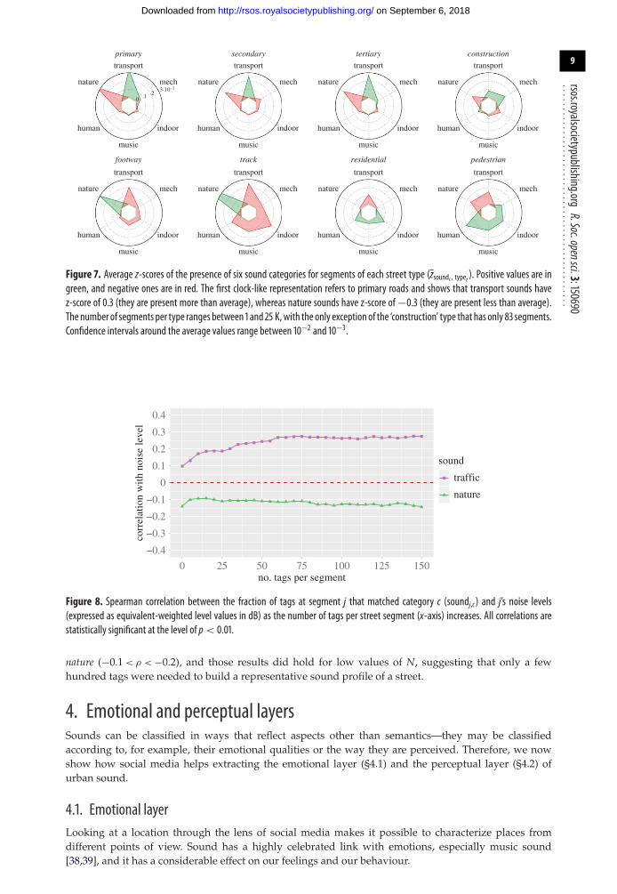
where St is the set of segments of (street) type t. Figure 7 reports the average values of those z-scores.Each clock-like representation refers to a street type, and the sound categories unfold along the clock:positive (negative) z-score values are marked in green (red) and suggest a presence of a sound categoryhigher (lower) than the average one. By looking at the positive values, we saw that primary, secondaryand tertiary streets (which contain cars) were associated with transport sounds; construction sites withmechanical sounds; footways and tracks (often embedded in parks) were associated with nature sounds;residential and pedestrian streets were associated with human, music and indoor sounds. Then, bylooking at the negative values, we learned that primary, secondary, tertiary and construction streetswere not associated with nature; and the other street types were not associated with sounds relatedto transport.

3.2. Noise pollutionThe most studied aspect of urban sounds is the issue of noise pollution. Despite the importance of thatissue, there are no reliable and high-coverage noise measurement data for world-class cities. There is agreat number of participatory sensing applications that manage databases of noise levels in several cities,and some of them are publicly accessible [8–12], but all of them offer a limited geographical coverage ofa city.

Barcelona is an exception, however. In 2009, the city council started a project, called Strategic NoiseMap, whose main goal was to monitor noise levels and ultimately find new ways of limiting soundpollution. The project has a public API6 that returns noise values at the level of street segment for thewhole city. For each segment, we collected the four dB values provided: three yearly averages for thethree times of the day (day: from 07.00 to 21.00; evening: from 21.00 to 23.00; and night: from 23.00 to07.00), and one aggregate value, the equivalent-weighted level (EWL), that averages those three valuesadding a 5 dB penalty to the evening period, and a 10 dB to the night period. With a practice akin to theone used for air quality indicators [34,35], those noise level values are estimated by a prediction modelthat is bootstrapped with field measurements [36]. In the case of Barcelona, the model is bootstrappedwith 2.300 short-span noise measurements lasting at most 15 min, usually taken during daytime, andwith 100 long-span ones lasting from 24 h to a few days.

To see whether noise pollution was associated with specific sound categories, we considered the streetsegments with at least N tags and computed, across all the segments, the Spearman rank correlationsρj(EWLj, soundj,c) between segment j’s EWL values (in dB) and j’s fraction of picture tags that matched

6Interactive Map of Noise Pollution in Barcelona (http://w20.bcn.cat:1100/WebMapaAcustic/mapa_soroll.aspx?lang=en).

on September 6, 2018http://rsos.royalsocietypublishing.org/Downloaded from

8

rsos.royalsocietypublishing.orgR.Soc.opensci.3:150690

................................................

1 – REGENT’S PARK2 – HYDE PARK3 – GREEN PARK4 – WATERLOO

5 – HYDE PARK CORNER6 – SOHO

7 – BLOOMSBURY8 – CAMDEN HIGH ST.

9 – RIVER THAMES

1 – MONTJUIC PARK2 – PARK GÜELL

3 – CIUTADELLA PARK

4 – AV. DIAGONAL

5 – PLAZA DE ESPAÑA6 – AV. DE LES CORTS CATALANES

7 – GOTHIC/CIUTAT VELLA

8 – BARCELONETA

9 – RONDA LITORAL (WATER FRONT)

10 – EL FORUM

transportnaturehumanmusicindoor

transportnaturehumanmusicindoor

1

8

7

6

3

5

9

2 6

410

93

78

5

6 1

4

2

4

9

9

(a)

(b)

Figure 6. Urban sound maps of London (a) and Barcelona (b). Each street segment is marked with the sound category c that has thehighest z-score for that segment (zsoundj,c ). In London, natural sounds are found in Regent’s Park (1), Hyde Park (2), Green Park (3) and allaround the River Thames (9). By contrast, transport sounds are aroundWaterloo station (4) and on the perimeter of Hyde Park (5). Humansounds are found in Soho (6) and Bloomsbury (7), and music is associated with the small clubs on Camden High Street (8). In Barcelona,natural sounds are found in Montjuic Park (1), Park Guell (2) and Ciutadella Park (3), and on the beaches of Barceloneta (8) and RondaLitoral (9). By contrast, annoying and chaotic sounds are found on the main road of Avinguda Diagonal (4), on Plaza de Espana (5) andon Avinguda De Les Corts Catalanes (6). Human sounds are found in the historical centre called Gothic/Ciutat Vella (7), and music in theopen-air arena of El Forum (10). Only segments with at least five sound tags were considered.

category c7 (figure 8). The idea was to determine not only which categories were associated with noisepollution but also how many tags were needed to have a significant association. We found that noisepollution was positively correlated (p < 0.01) with traffic (0.1 < ρ < 0.3) and negatively correlated with

7In computing the correlations, we used the method by Clifford et al. [37] to address spatial autocorrelations.

on September 6, 2018http://rsos.royalsocietypublishing.org/Downloaded from

9

rsos.royalsocietypublishing.orgR.Soc.opensci.3:150690

................................................transport

primary secondary tertiary construction

music

footway track residential pedestrian

mech

0 1 23·10–1

nature

indoorhuman

transport

music

mechnature

indoorhuman

transport

music

mechnature

indoorhuman

transport

music

mechnature

indoorhuman

transport

music

mechnature

indoorhuman

transport

music

mechnature

indoorhuman

transport

music

mechnature

indoorhuman

transport

music

mechnature

indoorhuman

Figure 7. Average z-scores of the presence of six sound categories for segments of each street type (z̄soundc , typet ). Positive values are ingreen, and negative ones are in red. The first clock-like representation refers to primary roads and shows that transport sounds havez-score of 0.3 (they are present more than average), whereas nature sounds have z-score of−0.3 (they are present less than average).The number of segments per type ranges between 1 and 25 K,with the only exception of the ‘construction’ type that has only 83 segments.Confidence intervals around the average values range between 10−2 and 10−3.

−0.4

−0.3

−0.2

−0.1

0

0.1

0.2

0.3

0.4

0 25 50 75 100 125 150no. tags per segment

corr

elat

ion

with

noi

se le

vel

sound

traffic

nature

Figure 8. Spearman correlation between the fraction of tags at segment j that matched category c (soundj,c) and j’s noise levels(expressed as equivalent-weighted level values in dB) as the number of tags per street segment (x-axis) increases. All correlations arestatistically significant at the level of p< 0.01.

nature (−0.1 < ρ < −0.2), and those results did hold for low values of N, suggesting that only a fewhundred tags were needed to build a representative sound profile of a street.

4. Emotional and perceptual layersSounds can be classified in ways that reflect aspects other than semantics—they may be classifiedaccording to, for example, their emotional qualities or the way they are perceived. Therefore, we nowshow how social media helps extracting the emotional layer (§4.1) and the perceptual layer (§4.2) ofurban sound.

4.1. Emotional layerLooking at a location through the lens of social media makes it possible to characterize places fromdifferent points of view. Sound has a highly celebrated link with emotions, especially music sound[38,39], and it has a considerable effect on our feelings and our behaviour.

on September 6, 2018http://rsos.royalsocietypublishing.org/Downloaded from

10

rsos.royalsocietypublishing.orgR.Soc.opensci.3:150690

................................................Table 1. Description of the eight most frequent street types in Open Street Map.

street type description

footway designated footpaths mainly or exclusively for pedestrians. This includes walking tracks and gravel paths. . . . . . . . . . . . . . . . . . . . . . . . . . . . . . . . . . . . . . . . . . . . . . . . . . . . . . . . . . . . . . . . . . . . . . . . . . . . . . . . . . . . . . . . . . . . . . . . . . . . . . . . . . . . . . . . . . . . . . . . . . . . . . . . . . . . . . . . . . . . . . . . . . . . . . . . . . . . . . . . . . . . . . . . . . . . . . . . . . . . . . . . . . . . . . . . . . . . . . . . . . . . . . . . . . . . . . . . .

residential roads that serve as an access to housing, without function of connecting settlements. Often lined with housing. . . . . . . . . . . . . . . . . . . . . . . . . . . . . . . . . . . . . . . . . . . . . . . . . . . . . . . . . . . . . . . . . . . . . . . . . . . . . . . . . . . . . . . . . . . . . . . . . . . . . . . . . . . . . . . . . . . . . . . . . . . . . . . . . . . . . . . . . . . . . . . . . . . . . . . . . . . . . . . . . . . . . . . . . . . . . . . . . . . . . . . . . . . . . . . . . . . . . . . . . . . . . . . . . . . . . . . . .

pedestrian roads used mainly or exclusively for pedestrians in shopping and residential areas. They may allow access ofmotorized vehicles only for very limited periods of the day

. . . . . . . . . . . . . . . . . . . . . . . . . . . . . . . . . . . . . . . . . . . . . . . . . . . . . . . . . . . . . . . . . . . . . . . . . . . . . . . . . . . . . . . . . . . . . . . . . . . . . . . . . . . . . . . . . . . . . . . . . . . . . . . . . . . . . . . . . . . . . . . . . . . . . . . . . . . . . . . . . . . . . . . . . . . . . . . . . . . . . . . . . . . . . . . . . . . . . . . . . . . . . . . . . . . . . . . . .

track roads for mostly agricultural or forestry uses. Tracks are often rough with unpaved surfaces. . . . . . . . . . . . . . . . . . . . . . . . . . . . . . . . . . . . . . . . . . . . . . . . . . . . . . . . . . . . . . . . . . . . . . . . . . . . . . . . . . . . . . . . . . . . . . . . . . . . . . . . . . . . . . . . . . . . . . . . . . . . . . . . . . . . . . . . . . . . . . . . . . . . . . . . . . . . . . . . . . . . . . . . . . . . . . . . . . . . . . . . . . . . . . . . . . . . . . . . . . . . . . . . . . . . . . . . .

primary a major highway linking large towns, normally with two lanes not separated by a central barrier. . . . . . . . . . . . . . . . . . . . . . . . . . . . . . . . . . . . . . . . . . . . . . . . . . . . . . . . . . . . . . . . . . . . . . . . . . . . . . . . . . . . . . . . . . . . . . . . . . . . . . . . . . . . . . . . . . . . . . . . . . . . . . . . . . . . . . . . . . . . . . . . . . . . . . . . . . . . . . . . . . . . . . . . . . . . . . . . . . . . . . . . . . . . . . . . . . . . . . . . . . . . . . . . . . . . . . . . .

secondary a highway which is not part of a major route, but nevertheless forming a link in the national route network,normally with two lanes

. . . . . . . . . . . . . . . . . . . . . . . . . . . . . . . . . . . . . . . . . . . . . . . . . . . . . . . . . . . . . . . . . . . . . . . . . . . . . . . . . . . . . . . . . . . . . . . . . . . . . . . . . . . . . . . . . . . . . . . . . . . . . . . . . . . . . . . . . . . . . . . . . . . . . . . . . . . . . . . . . . . . . . . . . . . . . . . . . . . . . . . . . . . . . . . . . . . . . . . . . . . . . . . . . . . . . . . . .

tertiary roads connecting smaller settlements or roads connecting minor streets to more major roads. . . . . . . . . . . . . . . . . . . . . . . . . . . . . . . . . . . . . . . . . . . . . . . . . . . . . . . . . . . . . . . . . . . . . . . . . . . . . . . . . . . . . . . . . . . . . . . . . . . . . . . . . . . . . . . . . . . . . . . . . . . . . . . . . . . . . . . . . . . . . . . . . . . . . . . . . . . . . . . . . . . . . . . . . . . . . . . . . . . . . . . . . . . . . . . . . . . . . . . . . . . . . . . . . . . . . . . . .

construction active road construction sites. Major road and rail construction schemes that typically require several years tocomplete

. . . . . . . . . . . . . . . . . . . . . . . . . . . . . . . . . . . . . . . . . . . . . . . . . . . . . . . . . . . . . . . . . . . . . . . . . . . . . . . . . . . . . . . . . . . . . . . . . . . . . . . . . . . . . . . . . . . . . . . . . . . . . . . . . . . . . . . . . . . . . . . . . . . . . . . . . . . . . . . . . . . . . . . . . . . . . . . . . . . . . . . . . . . . . . . . . . . . . . . . . . . . . . . . . . . . . . . . .

One way of extracting emotions from georeferenced content is to use a word-emotion lexiconknown as EmoLex [40]. This lexicon classifies words into eight primary emotions: it contains binaryassociations of 6468 terms with the their typical emotional responses. The eight primary emotions (anger,fear, anticipation, trust, surprise, sadness, joy and disgust) come from Plutchik’s psychoevolutionarytheory [41], which is commonly used to characterize general emotional responses. We opted for EmoLexinstead of other commonly used sentiment dictionaries (such as LIWC [42]) as it made it possible to studyfiner-grained emotions.

We matched our Flickr tags with the words in EmoLex and, for each street segment, we computed itsemotion profile. The profile consisted of all Plutchik’s primary emotions, in that each of its elements wasassociated with an emotion:

emotionj,e =tagj,e

tagj, (4.1)

where tagj,e is the number of tags at segment j that matched primary emotion e. We then computed thecorresponding z-score:

zemotionj,e = emotionj,e − μ(emotione)

σ (emotione). (4.2)

By computing the Spearman rank correlation ρj(zsoundj,c , zemotionj,e ), we determined which sound wasassociated with which emotion. From figure 9, we see that joyful words were associated with streetstypically characterized by music and human sounds, whereas they were absent in streets with traffic.Traffic was, instead, associated with words of fear, anticipation and anger. Interestingly, words of sadness(together with those of joy) were associated with streets with music, words of trust with indoors andwords of surprise with streets typically characterized by human sounds.

4.2. Perceptual layerFrom our social media data, we knew the extent to which a potential source of sound was present on astreet. If we knew how people usually perceived that source as well, we could have estimated how thestreet was likely to be perceived.

One way of determining how people usually perceive sounds in the city context is to run soundwalks.These were introduced in the late 1960s [43] and are still common among acoustic researchersnowadays [44,45]. Therefore, to determine people’s perceptions, one of the authors conducted soundwalksacross eight areas in Brighton and Hove (UK) and 11 areas in Sorrento (Italy) in April and October.They involved 37 participants (UK: 16 males, five females, μage = 38.6, δage = 11.5; Italy: 10 males, sixfemales, μage = 34.7, δage = 7.1) with a variety of backgrounds (e.g. acousticians, architects, planningprofessionals, local authorities and environmental officers). The experimenter led the participants alonga predefined route and stopped at selected locations. At each of the locations, participants were askedto listen to the acoustic environment for two minutes and to complete a structured questionnaire(table 2) inquiring about sound sources’ notability [46], soundscape attributes [46], overall soundscape

on September 6, 2018http://rsos.royalsocietypublishing.org/Downloaded from

11

rsos.royalsocietypublishing.orgR.Soc.opensci.3:150690

................................................joy

sadness

trust

fear

surprisedisgust

anger

anticipationjoy

sadness

trust

fear

surprisedisgust

anger

anticipationjoy

sadness

trust

fear

surprisedisgust

anger

anticipation

joy

sadness

trust

fear

surprisedisgust

anger

anticipationjoy

sadness

trust

fear

surprisedisgust

anger

anticipationjoy

sadness

trust

fear

surprisedisgust

anger

anticipation

transport nature human

music indoor mechanical

0 1 2 3 4·10–1

Figure 9. Correlation between zsoundj,c and zemotionj,e . Each clock-like representation refers to a sound category. The different emotionsunfold around the clock, and the emotions that are associated with the sound category are marked in green (positive correlations) orin red (negative emotions). All correlations are statistically significant at the level of p< 0.01.

Table 2. The questionnaire used during the soundwalk. For each question, participants could express their preference on a 10-pointordinal scale.

question items scale extremes (1–10)

to what extent do you presently hear thefollowing five types of sounds?

Traffic noise (e.g. cars, trains, planes), soundsof individuals (e.g. conversation, laughter,children at play), crowds of people (e.g.passers, sports event, festival), naturalsounds (e.g. singing birds, flowing water,wind in the vegetation), other noise (e.g.sirens, construction, industry)

[do not hear at all, . . .,dominates completely]

. . . . . . . . . . . . . . . . . . . . . . . . . . . . . . . . . . . . . . . . . . . . . . . . . . . . . . . . . . . . . . . . . . . . . . . . . . . . . . . . . . . . . . . . . . . . . . . . . . . . . . . . . . . . . . . . . . . . . . . . . . . . . . . . . . . . . . . . . . . . . . . . . . . . . . . . . . . . . . . . . . . . . . . . . . . . . . . . . . . . . . . . . . . . . . . . . . . . . . . . . . . . . . . . . . . . . . . . .

overall, how would you describe thepresent surrounding soundenvironment?

— [very bad, . . ., very good]

. . . . . . . . . . . . . . . . . . . . . . . . . . . . . . . . . . . . . . . . . . . . . . . . . . . . . . . . . . . . . . . . . . . . . . . . . . . . . . . . . . . . . . . . . . . . . . . . . . . . . . . . . . . . . . . . . . . . . . . . . . . . . . . . . . . . . . . . . . . . . . . . . . . . . . . . . . . . . . . . . . . . . . . . . . . . . . . . . . . . . . . . . . . . . . . . . . . . . . . . . . . . . . . . . . . . . . . . .

overall, to what extent is the presentsurrounding sound environmentappropriate to the present place?

— [not at all, . . ., perfectly]

. . . . . . . . . . . . . . . . . . . . . . . . . . . . . . . . . . . . . . . . . . . . . . . . . . . . . . . . . . . . . . . . . . . . . . . . . . . . . . . . . . . . . . . . . . . . . . . . . . . . . . . . . . . . . . . . . . . . . . . . . . . . . . . . . . . . . . . . . . . . . . . . . . . . . . . . . . . . . . . . . . . . . . . . . . . . . . . . . . . . . . . . . . . . . . . . . . . . . . . . . . . . . . . . . . . . . . . . .

for each of the eight scales below, to whatextent do you agree or disagree that thepresent surrounding soundenvironment is . . .

pleasant, chaotic, vibrant, uneventful, calm,annoying, eventful, monotonous

[strongly disagree, . . .,strongly agree]

. . . . . . . . . . . . . . . . . . . . . . . . . . . . . . . . . . . . . . . . . . . . . . . . . . . . . . . . . . . . . . . . . . . . . . . . . . . . . . . . . . . . . . . . . . . . . . . . . . . . . . . . . . . . . . . . . . . . . . . . . . . . . . . . . . . . . . . . . . . . . . . . . . . . . . . . . . . . . . . . . . . . . . . . . . . . . . . . . . . . . . . . . . . . . . . . . . . . . . . . . . . . . . . . . . . . . . . . .

quality [46,47] and soundscape appropriateness [48]. The questionnaire classified urban sounds intofive categories (traffic, individuals, crowds, nature, other) as it is typically done in soundwalks [49,50],and the perceptions of such sounds into eight categories (pleasant, chaotic, vibrant, uneventful, calm,annoying, eventful and monotonous, after Axelsson et al.’s [51] work).

Those soundwalks resulted in 342 tuples, each of which represents a participant’s report about soundsand perceptions at a given location. Each tuple had 13 [1,10] values: five values reflecting the extent towhich the five sound categories were reported to be present, and the other eight reflecting the extent towhich the eight perceptions were reported. More technically, soundk,c is the score for sound category cat tuple k, and perceptionk,f is the score for perception category f at tuple k. The frequency distributionsof soundk,c (figure 10) suggest that the participants experienced both streets with only a few sounds,and streets with many. In addition, they rarely experienced crowds and came across traffic and, only at

on September 6, 2018http://rsos.royalsocietypublishing.org/Downloaded from

12

rsos.royalsocietypublishing.orgR.Soc.opensci.3:150690

................................................

0

10

20

30

40

50

1 2 3 4 5 6 7 8 9 10

individuals

0

50

100

150

1 2 3 4 5 6 7 8 9 10

crowds

0

20

40

1 2 3 4 5 6 7 8 9 10

nature

0

20

40

60

80

1 2 3 4 5 6 7 8 9 10

traffic

0

20

40

60

1 2 3 4 5 6 7 8 9 10

other

Figure 10. Frequency distributions of the survey’s scores for sound presence (from 1 to 10) across categories: individuals, crowds, nature,traffic and other. Sounds of individuals are scored in the full 1-to-10 range, whereas sounds of crowds are typically scored with a value of1 or 2 as they might have been absent most of the time.

0

10

20

30

40

1 2 3 4 5 6 7 8 910

pleasant

01020304050

1 2 3 4 5 6 7 8 910

calm

0

20

40

60

1 2 3 4 5 6 7 8 910

vibrant

01020304050

1 2 3 4 5 6 7 8 910

eventful

0

20

40

1 2 3 4 5 6 7 8 910

annoying

0

20

40

60

1 2 3 4 5 6 7 8 910

chaotic

0

20

40

1 2 3 4 5 6 7 8 910

monotonous

0

20

40

60

1 2 3 4 5 6 7 8 910

uneventful

Figure 11. Frequency distributions of the survey’s perception scores (from 1 to 10) for each perception category. Most of the perceptionsare scored in the full 1-to-10 range.

times, nature. Instead, the frequency distributions of perceptionk,f (figure 11) suggest that the participantsexperienced streets with very diverse perceptual profiles, resulting in the use of the full [1,10] score rangefor all perceptions.

To see which sounds participants tended to experience together, we computed the rank cross-correlation ρk(soundk,c1 , soundk,c2 ) (figure 12a). Amid crowds, the participants reported high score inthe category ‘individuals’. These two sound categories—individuals and crowds—had similar soundprofiles so much so that the category ‘crowds’ could be experimentally replaced by the category‘individuals’ in the specific instance of those soundwalks. Furthermore, as one would expect, thepresence of traffic was associated with the absence of individuals, crowds and nature.

To then see which perceptions participants tended to experience together, we computed therank cross-correlation ρ(perceptionk,f1 , perceptionk,f2 ) (figure 12b). Perceptions meant to have oppositemeanings indeed resulted in negative correlations (pleasant versus annoying, eventful versusuneventful, vibrant versus monotonous and calm versus chaos). Interestingly, with their near-zero

on September 6, 2018http://rsos.royalsocietypublishing.org/Downloaded from

13

rsos.royalsocietypublishing.orgR.Soc.opensci.3:150690

................................................

crowds annoying

annoying

calm

calm

chaotic

chaotic

eventful

eventful

monotonous

monotonous

pleasant

pleasant

uneventful

uneventful

vibrant

vibrant

crowds

individuals

individuals

nature

nature

other

other

traffic

traffic

0.67

0.67

0.03

–0.01 –0.04 0.10 –0.03

–0.03–0.35–0.43–0.34

0.15 0.10 –0.35

0.15 –0.04 –0.43

0.03 –0.01 –0.34–0.73

–0.73

0.55

0.33

–0.79

0.07

–0.14 –0.03

0.20 –0.21

0.24 0.68 –0.44 0.20 –0.59

–0.76 0.42 –0.03 –0.59

0.76 –0.55 0.09 –0.31 –0.03 0.20

–0.17 0.01 –0.42 –0.31 0.42 –0.44

–0.03 –0.11 0.21 –0.42 0.09 –0.76 0.68

–0.68 0.21 0.01 –0.55 –0.21 0.24

–0.68 –0.11 –0.17 0.76 0.20 –0.03

0.55 0.33 –0.79 0.07 –0.14–0.03

(a) (b)

Figure 12. Pairwise rank cross-correlations between the survey’s sound scores soundk,c (a) and its perception scores perceptionk,e (b).

eventful

uneventful

annoying pleasant

CHAOTIC VIBRANT

CALMMONOTONOUS

Figure 13. Two principal components describing how study participants perceived urban sound. The combination of the first component‘uneventful versus eventful’ with the second component ‘annoying versus pleasant’ results in fourmainways of perceiving urban sounds:vibrant, calm, monotonous and chaotic [51].

annoyingcalm

chaotic

eventful

monotonous

pleasant

uneventful

vibrant

annoyingcalm

chaotic

eventful

monotonous

pleasant

uneventful

vibrant

crowds

individuals

nature

other

traffic

crowds

individuals

nature

other

traffic

–0.40 0.23 –0.09 0.33 –0.31 0.46 –0.24 0.46 0.03

0.03

0.06

0.23

0.29

0.20

0.23

0.34

0.09

0.03

0.10

0.11

0.05

0.22

0.32

0.06

0.06

0.08

0.23

0.19

0.25

0.24

0.30

0.07

0.03

0.06

0.06

0.16

0.23

0.14

0.31

0.28

0.16

0.16

0.10

0.22

0.17

0.13

0.16

0.14

0.38–0.180.52–0.290.30–0.220.38–0.49

–0.31 0.47 –0.40 –0.10 0.00 0.39 0.17 –0.11

–0.010.14–0.24–0.260.010.15–0.170.29

0.57 –0.61 0.56 0.07 0.16 –0.64 –0.14 –0.08

(a) (b)

Figure 14. Relationship between sounds and perceptions in the soundwalk survey data. (a) Correlations between the survey’s soundscores soundk,c and its perception scores perceptionk,e. Sounds of crowds, for example, are perceived to be pleasant and vibrant but notannoying. (b) Probability p(f |c) that perception f was reported at a location with sound category c.

correlation, pleasantness and eventfulness were orthogonal—when a place was eventful, nothing couldhave been said about its pleasantness.

To see which sounds participants experienced together with which perception, we computed the rankcorrelation ρk(soundk,c, perceptionk,f ) (figure 14a). On average, vibrant areas tended to be associated withcrowds, pleasant areas with individuals, calm areas with nature and annoying and chaotic areas with

on September 6, 2018http://rsos.royalsocietypublishing.org/Downloaded from

14

rsos.royalsocietypublishing.orgR.Soc.opensci.3:150690

................................................1 – REGENT’S PARK

2 – HYDE PARK

3 – GREEN PARK

4 – WATERLOO

5 – HYDE PARK CORNER

6 – SOHO

7 – BLOOMSBURY

9 – RIVER THAMES

8 – CAMDEN HIGH ST.

chaoticcalmmonotonousvibrant

chaoticcalmmonotonousvibrant

1 – MONTJUIC PARK

2 – PARK GÜELL

3 – CIUTADELLA PARK

4 – AV. DIAGONAL

5 – PLAZA DE ESPAÑA

6 – AV. DE LES CORTS CATALANES

7 – GOTHIC/CIUTAT VELLA

9 – RONDA LITORAL (WATER FRONT)

10 – EL FORUM

8 – BARCELONETA

2

5

34

9

7

6

1

8

9

9

2

4

5

6 1

78

39

410

6

(b)

(a)

Figure 15. Perceptualmaps of London (a) andBarcelona (b). At each segment, the perception f with the highest probabilitywas reported(i.e. with the highest pj(f )). In London, calm soundswere found in Regent’s Park (1), Hyde Park (2), Green Park (3) and all around the RiverThames (9). By contrast, chaotic sounds were around Waterloo station (4) and Hyde Park Corner (5). Vibrant sounds were found in Soho(6), Bloomsbury (7) and Camden High Street (8). In Barcelona, calm sounds were found in Montjuic Park (1), Park Guell (2) and CiutadellaPark (3), and on the beach of Barceloneta (8). By contrast, on the beach in front of Ronda Litoral (9), we found monotonous sounds.Chaotic sounds were found on the main road of Avinguda Diagonal (4), on Plaza de Espana (5) and on Avinguda De Les Corts Catalanes(6). Vibrant sounds were found in the historical centre called Gothic/Ciutat Vella (7), and some in the open-air arena of El Forum (10),which was also characterized by chaotic sounds.

traffic. In a similar way, Axelsson et al. studied the principal components of their perceptual data [51]and found very similar results: they found that two components best explain most of the variability inthe data (figure 13).

Finally, to map how streets are likely to be perceived, we needed to estimate a street’s expectedperception given the street’s sound profile. The sound profiles came from our social media data,whereas the expected perception could have been computed from our soundwalks’ data. We had alreadycomputed the correlations between sounds and perceptions (figure 14a). However, those correlations arenot expected values (accounting for, e.g. whether a perception is frequent or rare) but they simply are

on September 6, 2018http://rsos.royalsocietypublishing.org/Downloaded from

15

rsos.royalsocietypublishing.orgR.Soc.opensci.3:150690

................................................(b)(a) (c)

Figure 16. Examples of ambiguously tagged pictures. (a) Street art in Brick Lane taggedwith the term ‘screaming’, and the same locationCarriage Drive with Hyde Park tagged with opposing terms related to (b) traffic sounds and (c) nature sounds.

strength measures. Therefore, we computed the probability of perception f given sound category c as

p( f |c) = p(c| f ) · p( f )p(c)

. (4.3)

To compute the composing probabilities, we needed to discretize our [1,10] values taken during thesoundwalks, and did so by segmenting them into quartiles. We then computed

p(c| f ) = Q4(c ∧ f )Q4( f )

(4.4)

and

p(c) = Q4(c)Q4(c∗)

; p( f ) = Q4( f )Q4( f ∗)

, (4.5)

where Q4(c) is the number of times the sound category c occurred in the fourth quartile of its score;Q4(c∗) is the number of times any sound occurred in its fourth quartile; and Q4(c ∧ f ) is the number oftimes sound c as well as perception f occurred in their fourth quartiles.

The conclusions drawn from the resulting conditional probabilities (figure 14b) did not differ fromthose drawn from the previously shown sound–perception correlations (figure 14a). As opposed to thecorrelation values, none of the conditional probabilities were very high (all below 0.33). This is becausethe conditional probabilities were estimated through the gathering of perceptual data in the wild8 and,as such, the mapping between perception and sound did not result in fully fledged probability values.Those values are best interpreted not as raw values but as ranked values. For example, nature soundswere associated with calm only with a probability 0.34, yet calm is the strongest perception related tonature as it ranks first.

The advantage of conditional probabilities over correlations is that they offer principled numbers thatare properly normalized and could be readily used in future studies. They could be used, for example, todraw an aesthetics map, a map that reflects the emotional qualities of sounds. In the maps of figure 15,we associated each segment with the colour corresponding to the perception with the highest value ofpj( f ) = ∑

c p( f |c) · pj(c), where pj(c) = soundj,c, which is the fraction of tags at segment j that matchedsound category c. pj( f ) is effectively the probability that perception f is associated with street segmentj, and the strongest f is associated with j. By mapping the probabilities of sound perceptions in London(figure 15a) and Barcelona (figure 15b), we observed that trafficked roads were chaotic, whereas walkableparts of the city were exciting. More interestingly, in the soundscape literature, monotonous areas havenot necessarily been considered pleasant (they fall into the annoying quadrant of figure 13), yet thebeaches of Barcelona were monotonous (and rightly so), but might have also been pleasant.

5. DiscussionA project called SmellyMaps mapped urban smellscapes from social media [25], and this work—calledChattyMaps—has three main similarities with it. First, the taxonomy of sound and that of smell were

8It has been shown that, in soundwalks, perception ratings are affected by not only sounds, but also visual cues (e.g. greenery has beenfound to modulate soundscape ‘tranquillity’ ratings [52,53]).

on September 6, 2018http://rsos.royalsocietypublishing.org/Downloaded from

16

rsos.royalsocietypublishing.orgR.Soc.opensci.3:150690

................................................

0

0.05

0.10

0.15

0 0.5 1.0 1.5 2.0 2.5 3.0segment tag entropy

prob

abili

ty

0

0.5

1.0

1.5

2.0

1 25 50 75 100 125 150no. sound tags per segment

segm

ent t

ag e

ntro

py

city

London

Barcelona

Figure 17. Diversity (entropy) of sound tags. Frequency distribution (a), and how the diversity varies with the number of tags per streetsegment (b). Segments with zero diversity (28% in Barcelona, 35% in London) were excluded.

low high

low high

(b)

(a)

Figure 18. Maps of the diversity of sound tags for each street segment in London (a) and Barcelona (b). Only segments with five ormoretags are displayed.

on September 6, 2018http://rsos.royalsocietypublishing.org/Downloaded from

17

rsos.royalsocietypublishing.orgR.Soc.opensci.3:150690

................................................both created using community detection algorithms, and both closely resembled categorizations widelyused by researchers and practitioners in the corresponding fields. Second, the ways that social mediadata were mapped onto streets (e.g. buffering of segments, use of longitude/latitude coordinates on thepictures) are the same. Third, in both works, the validation was done with official data (i.e. with airquality data and noise pollution data). However, the two works differ as well, and they do so in threemain ways. First, as opposed to SmellyMaps, ChattyMaps studied a variety of urban layers: not only theurban sound layer, but also the emotional, perceptual and sound diversity layers. Second, smell wordswere derived from smellwalks (as no other source was available), whereas sound words were derivedfrom the online platform of Freesound. Third, because SmellyMaps showed that picture tags were moreeffective than tweets in capturing geographical-salient information, ChattyMaps entirely relied on Flickrtags.

Our approach comes with a few limitations, mainly because of data biases. The urban soundscapeis multifaceted: the sounds we hear and the way we perceive them change considerably with smallvariations of, for example, space (e.g. simply turning a corner) and time (e.g. day versus night). Bycontrast, social media data have limited resolution and coverage, and that results in false positives. Attimes, sound tags do not reflect real sounds because of either misannotations or the figurative use of tags(figure 16a). Fortunately, those cases occur rarely. By manually inspecting 100 photos with sound tags, nofalse-positive was found: 87 pictures were correctly tagged and 13 referred to sounds that were plausibleyet hard to ascertain.

Even when tags refer to sounds likely present in an area, they might do so partially. For example,the tags on the picture of figure 16b consisted of traffic terms (rightly) but not of nature terms, and thatwas a partial view of that street’s soundscape. This risk shrinks as the number of sound tags for thesegment increases. Indeed, let us stick with the same example: figure 16c was taken a few metres awayfrom figure 16b, and its tags consisted of nature terms.

To partly mitigate noise at boundary regions, we did two things. First, as described in §2, we added abuffer of 22.5 m around each segment’s bounding box. This has been commonly done in previous workdealing with georeferenced digital content [25,26]. It is hard to measure automatically how many tagsare needed to get high confidence sound profiles, but we estimated it to be around 20–25 tags (figure 8),if official air quality data are used for validation.

Second, we associated sound distributions (and not individual sounds) with street segments. The six-dimensional sound vector was normalized in [0, 1] to have a probabilistic interpretation. In figure 16b,c,nature sounds were predominant, yet traffic-related sounds varied from 20% to 2% depending on thedifferent parts of that street.

More generally, to have a more comprehensive view of this phenomenon, we determined eachsegment’s sound diversity by computing the Shannon index

diversityj = −∑

csoundj,c · ln(soundj,c), (5.1)

where soundj,c is the fraction of tags at segment j that matched sound category c. After removing zerodiversity values (often associated with segments having only one tag, which made 28% of segments inBarcelona, and 35% segments in London), we saw that the frequency distribution of diversity (figure 17a)had two peaks in 1 (for both cities) and in 1.5 for London and in 2.0 for Barcelona. Then, by mappingthose values (figure 18), we saw that the values close to the first peak were associated with parks andsuburbs, and those close to the second peak (and higher) were associated with the central parts of thetwo cities. Furthermore, the diversity did not depend on the number of tags per segment and becamestable for segments with at least 10 tags (figure 17b).

6. ConclusionWe showed that social media data make it possible to effectively and cheaply track urban sounds at scale.Such a tracking was effective, because the resulting sounds were geographically sorted across street typesin expected ways, and they matched noise pollution levels. The tracking was also cheap because it didnot require the creation of any additional service or infrastructure. Finally, it worked at the scale of anentire city, and that is important, not least because, before our work, there had been nothing in sonographycorresponding to the instantaneous impression which photography can create . . . The microphone samples detailsand gives the close-up but nothing corresponding to aerial photography [16].

However, whereas landscapes can be static, soundscapes are dynamic [54]. Their perceptions areaffected by demography (e.g. personal sensitivity to noise, age), context (e.g. city layout) and time

on September 6, 2018http://rsos.royalsocietypublishing.org/Downloaded from

18

rsos.royalsocietypublishing.orgR.Soc.opensci.3:150690

................................................(e.g. day versus night, weekdays versus weekends). Future studies could partly address those issuesby collecting additional data and by comparing models of urban sounds generated from social mediawith those generated from geographic information system techniques.

Nonetheless, no matter what data one has, fully capturing soundscapes might well be impossible. Ourwork has focused on identifying potential sonic events. To use a food metaphor, if those events are theraw ingredients, then the aural architecture (which comes with the acoustic properties of trees, buildings,streets) is the cooking style, and the soundscape is the dish [54].

To unite hitherto isolated studies in a new synergy, in the future, we will conduct a comprehensivemulti-sensory research of cities, one in which visual [55,56], olfactory [25] and sound perceptions areexplored together.

The ultimate goal of this work is to empower city managers and researchers to find solutions for anecologically balanced soundscape where the relationship between the human community and its sonic environmentis in harmony, as Schafer famously (and prophetically) remarked in the late 1970s [16].

Data accessibility. Aggregate version of the data is available at http://goodcitylife.org and on Dryad doi:10.5061/dryad.tg735.Competing interests. We declare we have no competing interests.Funding. F.A. received funding through the People Programme (Marie Curie Actions) of the European Union’s 7thFramework Programme FP7/2007-2013 under REA grant agreement no. 290110, SONORUS ‘Urban Sound Planner’.Acknowledgements. We thank the Barcelona City Council for making the noise pollution data available.

References

1. Halonen J et al. 2015 Road traffic noise is associatedwith increased cardiovascular morbidity andmortality and all-cause mortality in London. Eur.Heart J. 36, 2653–2661. (doi:10.1093/eurheartj/ehv216)

2. Stansfeld SA et al. 2005 Aircraft and road trafficnoise and children’s cognition and health: across-national study. Lancet 365, 1942–1949.(doi:10.1016/S0140-6736(05)66660-3)

3. Van Kempen E, Babisch W. 2012 The quantitativerelationship between road traffic noise andhypertension: a meta-analysis. J. Hypertens. 30,1075–1086. (doi:10.1097/HJH.0b013e328352ac54)

4. Hoffmann B et al. 2006 Residence close to hightraffic and prevalence of coronary heart disease.Eur. Heart J. 27, 2696–2702. (doi:10.1093/eurheartj/ehl278)

5. Selander J, Nilsson ME, Bluhm G, Rosenlund M,Lindqvist M, Nise G, Pershagena G. 2009 Long-termexposure to road traffic noise and myocardialinfarction. Epidemiology 20, 272–279. (doi:10.1097/EDE.0b013e31819463bd)

6. The European Parliament. 2002 Directive2002/49/EC: assessment and managementof environmental noise. Off. J. Eur. Commun.189.

7. Morley D, De HK, Fecht D, Fabbri F, Bell M, GoodmanP, Elliott P, Hodgson S, Hansell A, Gulliver J. 2015International scale implementation of theCNOSSOS-EU road traffic noise prediction model forepidemiological studies. Environ. Pollut. 206,332–341. (doi:10.1016/j.envpol.2015.07.031)

8. Maisonneuve N, Stevens M, Niessen ME, Hanappe P,Steels L. 2009 Citizen noise pollution monitoring.In Proc. 10th Annual Int. Conf. on Digital GovernmentResearch, Puebla, Mexico, 17–21 May 2009, pp.96–103. Digital Government Society of NorthAmerica.

9. Schweizer I, Bärtl R, Schulz A, Probst F, MühläuserM. 2011 NoiseMap—real-time participatory noisemaps. In Proc. 2nd Int. Workshop on Sensing

Applications on Mobile Phones, Seattle, WA, USA,1 November 2011, pp. 1–5.

10. Meurisch C, Planz K, Schäfer D, Schweizer I. 2013Noisemap: discussing scalability in participatorysensing. In Proc. ACM 1st Int. Workshop on Sensingand Big Data Mining, Rome, Italy, 14 November 2013,pp. 6:1–6:6.

11. Becker M et al. 2013 Awareness and learning inparticipatory noise sensing. PLoS ONE 8, e81638.(doi:10.1371/journal.pone.0081638)

12. Mydlarz C, Nacach S, Park TH, Roginska A. 2014 Thedesign of urban sound monitoring devices. In AudioEngineering Society Convention 137, Los Angeles, CA,USA, 9–12 October 2014.

13. Hsieh H-P, Yen T-C, Li C-T. 2015 What makes NewYork so noisy?: reasoning noise pollution by miningmultimodal geo-social big data. In Proc. 23rd ACMInt. Conf. on Multimedia (MM), Brisbane, Australia,26–30 October 2015, pp. 181–184.

14. Nilsson ME, Berglund B. 2006 Soundscape quality insuburban green areas and city parks. Acta Acust.United with Acust. 92, 903–911.

15. Andringa TC, Lanser JJL. 2013 How pleasant soundspromote and annoying sounds impede health: acognitive approach. Int. J. Environ. Res. Public Health10, 1439–1461. (doi:10.3390/ijerph10041439)

16. Schafer RM. 1993 The soundscape: our sonicenvironment and the tuning of the world. Rochester,VT: Destiny Books.

17. International Organization for Standardization. 2014ISO 12913-1:2014 acoustics—Soundscape—part 1:definition and conceptual framework. Geneva,Switzerland: ISO.

18. Salamon J, Jacoby C, Bello JP. 2014 A dataset andtaxonomy for urban sound research. In Proc. 22ndACM Int. Conf. on Multimedia (MM), Orlando, FL,USA, 3–7 November 2014, pp. 1041–1044.

19. Salamon J, Bello J. 2015 Unsupervised featurelearning for urban sound classification. In IEEE Int.Conf. on Acoustics, Speech and Signal Processing,Brisbane, Australia, 19–24 April 2015, pp. 171–175.(doi:10.1109/ICASSP.2015.7177954)

20. Aletta F, Axelsson Ö, Kang J. 2014 Towards acousticindicators for soundscape design. In Proc. ForumAcusticum Conf., Krakow, Poland, 7–12 September2014.

21. Herranz-Pascual K, Aspuru I, Garcia I. 2010 Proposedconceptual model of environment experience asframework to study the soundscape. In Inter Noise2010: Noise and Sustainability, Lisbon, Portugal,13–16 June 2010, pp. 2904–2912. Institute of NoiseControl Engineering.

22. Schulte-Fortkamp B, Dubois D. 2006 Preface tospecial issue: recent advances in soundscaperesearch. Acta Acust. United with Acust. 92, I–VIII.

23. Schulte-Fortkamp B, Kang J. 2013 Introduction tothe special issue on soundscapes. J. Acoust. Soc. Am.134, 765–766. (doi:10.1121/1.4810760)

24. Davies WJ. 2013 Editorial to the special issue:applied soundscapes. Appl. Acoust. 2, 223.

25. Quercia D, Aiello LM, Schifanella R, McLean K. 2015Smelly maps: the digital life of urban smellscapes.In Int. AAAI Conf. onWeb and Social Media (ICWSM),Oxford, UK, 26–29 May 2015.

26. Quercia D, Aiello LM, Schifanella R, Davies A. 2015The digital life of walkable streets. In Proc. 24th ACMConf. onWorld WideWeb (WWW), Florence, Italy,18–22 May 2015, pp. 875–884.

27. Blei DM, Ng AY, Jordan MI. 2003 Latent dirichletallocation. J. Mach. Learn. Res. 3, 993–1022.

28. Lloyd SP. 1982 Least squares quantization in PCM.IEEE Trans. Inf. Theory 28, 129–137. (doi:10.1109/TIT.1982.1056489)

29. Fortunato S. 2010 Community detection in graphs.Phys. Rep. 486, 75–174. (doi:10.1016/j.physrep.2009.11.002)

30. Rosvall M, Bergstrom CT. 2008 Maps of randomwalks on complex networks reveal communitystructure. Proc. Natl Acad. Sci. USA 105, 1118–1123.(doi:10.1073/pnas.0706851105)

31. Blondel VD, Guillaume J-L, Lambiotte R, Lefebvre E.2008 Fast unfolding of communities in largenetworks. J. Stat. Mech. Theory Exp. 2008, P10008.(doi:10.1088/1742-5468/2008/10/P10008)

on September 6, 2018http://rsos.royalsocietypublishing.org/Downloaded from

19

rsos.royalsocietypublishing.orgR.Soc.opensci.3:150690

................................................32. Newman ME. 2006 Modularity and community

structure in networks. Proc. Natl Acad. Sci. USA103, 8577–8582. (doi:10.1073/pnas.0601602103)

33. Brown A, Kang J, Gjestland T. 2011 Towardsstandardization in soundscape preferenceassessment. Appl. Acoust. 72, 387–392.(doi:10.1016/j.apacoust.2011.01.001)

34. Eeftens M et al. 2012 Development of land useregression models for PM2.5 , PM2.5 absorbance,PM10 and PMcoarse in 20 European study areas;results of the ESCAPE project. Environ. Sci. Technol.46, 11195–11205. (doi:10.1021/es301948k)

35. Beelen R et al. 2013 Development of NO2 and NOxland use regression models for estimating airpollution exposure in 36 study areas inEurope—the ESCAPE project. Atmos. Environ. 72,10–23. (doi:10.1016/j.atmosenv.2013.02.037)

36. Gulliver J et al. 2015 Development of an open-sourceroad traffic noise model for exposure assessment.Environ. Model. Softw. 74, 183–193. (doi:10.1016/j.envsoft.2014.12.022)

37. Clifford P, Richardson S, Hémon D. 1989 Assessingthe significance of the correlation between twospatial processes. Biometrics 45, 123–134.(doi:10.2307/2532039)

38. Kivy P. 1989 Sound sentiment: an essay on themusical emotions, including the complete textof the corded shell. Philadelphia, PA: TempleUniversity Press.

39. Zentner M, Grandjean D, Scherer KR. 2008 Emotionsevoked by the sound of music: characterization,classification, and measurement. Emotion 8, 494.(doi:10.1037/1528-3542.8.4.494)

40. Mohammad SM, Turney PD. 2013 Crowdsourcing aword–emotion association lexicon. Comput. Intell.29, 436–465. (doi:10.1111/j.1467-8640.2012.00460.x)

41. Plutchik R. 1991 The emotions. Lanham, MD:University Press of America.

42. Pennebaker J. 2013 The secret life of pronouns: whatour words say about us. New York, NY: Bloomsbury.

43. Southworth M. 1969 The sonic environment ofcities. Environ. Behav. 1, 49–70. (doi:10.1177/001391656900100104)

44. Semidor C. 2006 Listening to a city with thesoundwalk method. Acta Acust. United with Acust.92, 959–964.

45. Jeon JY, Hong JY, Lee PJ. 2013 Soundwalk approachto identify urban soundscapes individually. J.Acoust. Soc. Am. 134, 803–812. (doi:10.1121/1.4807801)

46. Axelsson Ö, Nilsson ME, Berglund B. 2009 A Swedishinstrument for measuring soundscape quality. InProc. Euronoise Conf., Edinburgh, UK, 26–28 October2009.

47. Liu J, Kang J, Luo T, Behm H, Coppack T. 2013Spatiotemporal variability of soundscapes in amultiple functional urban area. Landsc. UrbanPlann. 115, 1–9. (doi:10.1016/j.landurbplan.2013.03.008)

48. Axelsson Ö. 2015 How to measure soundscapequality. In Proc. Euronoise Conf., Maastricht, TheNetherlands, 31 May–3 June 2015, pp. 1477–1481.

49. Aletta F, Margaritis E, Filipan K, Romero VP,Axelsson Ö, Kang J. 2015 Characterization of thesoundscape in Valley Gardens, Brighton, by asoundwalk prior to an urban design intervention.

In Proc. Euronoise Conf., Maastricht, The Netherlands,31 May–3 June 2015, pp. 1–12.

50. Aletta F, Kang J. 2015 Soundscape approachintegrating noise mapping techniques: a case studyin Brighton, UK. Noise Mapp. 2, 50–58. (doi:10.1515/noise-2015-0001)

51. Axelsson Ö, Nilsson ME, Berglund B. 2010 A principalcomponents model of soundscape perception. J.Acoust. Soc. Am. 128, 2836–2846. (doi:10.1121/1.3493436)

52. Watts GR, Pheasant RJ, Horoshenkov KV. 2011Predicting perceived tranquillity in urban parks andopen spaces. Environ. Plann. B 38, 585–594.(doi:10.1068/b36131)

53. Watts G, Miah A, Pheasant R. 2013 Tranquillity andsoundscapes in urban green spaces: predicted andactual assessments from a questionnaire survey.Environ. Plann. B 40, 170–181. (doi:10.1068/b38061)

54. Blesser B, Salter L. 2009 Spaces speak, are youlistening? Experiencing aural architecture.Cambridge, MA: MIT Press.

55. Quercia D, Schifanella R, Aiello LM. 2014 Theshortest path to happiness: recommendingbeautiful, quiet, and happy routes in the city.In Proc. 25th ACM Conf. on Hypertext and SocialMedia (HT), Santiago, Chile, 1–4 September 2014,pp. 116–125.

56. Quercia D, O’Hare NK, Cramer H. 2014 Aestheticcapital: what makes London look beautiful, quiet,and happy? In Proc. 17th ACM Conf. on ComputerSupported Cooperative Work & Social Computing(CSCW), Baltimore, MD, USA, 15–19 February 2014,pp. 945–955.

on September 6, 2018http://rsos.royalsocietypublishing.org/Downloaded from