1

Charge, geometry, and effective mass in the Kerr-

Newman solution to the Einstein field equations

Gerald E. Marsh

Argonne National Laboratory (Ret)5433 East View ParkChicago, IL 60615

E-mail: gemarsh@uchicago.edu

Abstract. It has been shown that for the Reissner-Nordström solution to

the vacuum Einstein field equations charge, like mass, has a unique space-

time signature [Found. Phys. 38, 293-300 (2008)]. The presence of charge

results in a negative curvature. This work, which includes a discussion of

effective mass, is extended here to the Kerr-Newman solution.

PACS: 04.20.Cv, 04.20.Dw.

Key Words: Kerr-Newman, charge, curvature.

2

Introduction.

It has been shown in the predecessor to this paper [1] that if the source of the field

is the singularity of the vacuum Reissner-Nordström solution of the coupled Einstein-

Maxwell field equations, only the Schwarzschild mass is seen at infinity, with the charge

and its electric field making no contribution. It was also shown that if the charge alone is

the source of the field, the effective mass seen at infinity vanishes. These results are a

direct consequence of charge having the properties of a negative mass while the electric

field produced by the charge has a positive effective mass. Near the time-like singularity,

which is the source of the field, space-time has a negative curvature. The effective mass

within a sphere of radius R was found to be

M Eff

In= m − Q

2

R . (1)

On the other hand, the effective mass of the electric field outside this sphere is given by

M Eff

Out=

Q2

R . (2)

This results in

M Eff

In+ M Eff

Out= m. (3)

Thus, the “negative mass” associated with the charge Q is exactly compensated by the

effective mass contained in the electric field present in the volume exterior to the surface

r = R. If the radius r = R→∞, the effective mass contained within the surface at infinity

is m, the Schwarzschild or, equivalently, the ADM mass.

These results are extended here to the Kerr-Newman solution. Because of the

axial rather than spherical symmetry, the situation is far more complex than in the case of

the Reissner-Nordström solution. The Kerr-Newman solution to the field equations is, of

3

course, the charged Kerr solution, and like the Kerr solution, is asymptotically flat.

Being axially symmetric, it has two independent, commuting Killing vectors and these

have been used [2, 3, 4] in Komar’s formula [5] to derive conserved quantities.

The next section addresses the question of spatial curvature near the singularity

and this is followed by a discussion of effective mass.

Curvature in the Kerr-Newman solution

Vacuum solutions to the Einstein field equations satisfy Rµν = 0, and this means

that the curvature scalar R = Rµµ also vanishes. As a consequence, how best to

characterize the curvature near black holes is unclear. The Kretschmann scalar

K = RαβγδRαβγδ has been used by several authors [6, 7], but the interpretation of the scalar

is somewhat ambiguous. As pointed out in [7], the Kretschmann scalar can be positive

for spaces having a negative curvature. A different method of characterizing the

curvature that was used in [1] will be explored below.

The Kerr-Newman solution in generalized Eddington coordinates [8], which are

convenient for this approach, is given by

ds2

= dr2

− 2a sin2θ dr dφ + r2 + a2 sin

2θ dφ 2

+ r2 + a2 cos2θ dθ 2 − dt2

+2mr − Q

2

r2 + a2 cos2θ

dr − a sin2θ dφ + dt

2

,

(4)

where the symbols have their conventional meanings.

In [1] it was pointed out that for the Reissner-Nordström solution the metric takes

the Minkowski form when r = Q2/2m. Interestingly enough, the same thing occurs in the

Kerr-Newman metric except that now r has a different meaning with surfaces of constant

r corresponding to confocal ellipsoids satisfying

x2 + y2

r2 + a2 + z2

r2 = 1. (5)

4

It will be seen, however, that unlike the Reissner-Nordström solution, where it

was possible to show that for r < Q2/2m the curvature was negative, the case of the Kerr-

Newman solution is more complex.

In order to interpret what follows, it will be necessary to compute the surfaces

where grr and gφφ vanish; the infinite red shift surfaces (where g00 = 0) for various values

of the parameters, and their relation to the horizons, have been given elsewhere [9] and

are not relevant to the following discussion. To determine the curvature near the ring

singularity, it is useful to examine the case where a2 + Q2 > m2, which allows the region

near the singularity to be visible from infinity. Setting a = m = Q = 1 as a convenient

choice of parameters, the condition gφφ = 0 results in the fourth order equation

r4 + r2 + r2 + 1 cos2θ + 2r − 1 sin

2θ = 0. (6)

Two of the solutions to this equation are imaginary, one is negative, and the last is

positive and real. The latter is very long and writing it out would add no insight into its

nature. The condition grr = 0 using the same value for the parameters results in the

quadratic equation

r2 + 2r + cos2θ − 1 = 0. (7)

The positive root is r = 2 − cos2θ − 1 . While the surface grr = 0 will play no role in

what follows, it and its relation to the surface gφφ = 0 are of interest in their own right.

The plots of the real, positive solution to Eq. (6) and of Eq. (7) are shown in Cartesian

coordinates in Fig. 1, where henceforth R = (x2 +y2)1/2. gφφ and grr are negative (time-like)

within their respective toroids gφφ = 0 and grr = 0.

5

Figure 1. The surfaces where grr = 0 and gφφ = 0 in Cartesian coordinates. Thevalues of the parameters are a = m = Q = 1. The surfaces are toroids, the z-axisbeing the axis of symmetry. The ring singularity is shown as a heavy dot locatedat R = 1 and z = 0.

The method of exploring the curvature near the ring singularity is the same as that

used in [1] where the ratio of the circumference of a circle to its radius was computed.

One has, for the Eddington coordinates used in Eq. (4), the relations

R = r2 + a212 sin θ and z = r cos θ. (8)

Notice that substituting these equations into Eq. (5) yields an identity.

First consider the equatorial plane where θ = π/2. The first of Eqs (8) allow the

ratio of the circumference of a circle in the plane to its radius to be written as

CR =

gφφ0

2πdφ

r2 + a212

= 2π

2mr − Q2

a2

r2 + r2 + a2

r2 + a2

12

.

(9)

Note that when C/R is set equal to 2π and the resulting equation solved for r one obtains

r = Q2/2m where the metric of Eq. (4) takes the Minkowski form. This ratio is plotted in

Fig. (2) for the same values of the parameters used in Fig. (1). The ratio vanishes for

6

r~0.404698, which corresponds to R~1.0830 in Cartesian coordinates. The toroidal

surface gφφ = 0 of Fig. 1 intersects the equatorial plane in two circles. The latter values of

r or R correspond to the circle of greatest radius.

Figure 2. The ratio of the circumference to the radius R in the equatorial plane ofthe Kerr-Newman solution in Eddington coordinates. The ring singularity isshown as the heavy dot at r = 0. The portion of the curve above the line C/R =2π corresponds to a negative curvature and that below to positive curvature. C/R= 0 at r ~ 0.404698 where gφφ = 0, and crosses the line C/R = 2π at r = Q2/2m,which for the value of the parameters used here, a = m = Q = 1, is 0.5.

The ratio of the circumference to its radius for a circle not in the equatorial plane

is considerably more complicated. Using both of Eqs. (8), the ratio can be written as a

function of the variables θ and z as

CR =

gφφ0

2πdφ

r2 + a212sin θ

=

2π2mz cos θ − Q

2cos2 θ a2sin

4 θ

z2 + cos4 θ+ z2 + a2cos2 θ tan

2 θ

12

z2 + a2cos2 θ12tan θ

.

(10)

7

For a given plane z = Const., each value of θ determines a circle in the plane centered on

the z-axis, corresponding to the intersection of that plane with the hyperboloid of one

sheet associated with each θ. These hyperbolae are confocal to the ellipsoids

corresponding to r = Const. given by Eq. (5). There is a bit of a subtlety here in that the

surface θ = Const. is only a half-hyperboloid lying in the half space z > 0 (z < 0) when

θ < π/2 (θ > π/2).

Note again that if z = r cosθ is substituted back into the expression for C/R given

by Eq. (10), and the result set equal to 2π, the solution to the equation for r again yields

r = Q2/2m independent of θ. The plots for various values of z are shown in Figs. 3(a),

3(b), and 3(c).

(a) (b) (c)

Figure 3. The ratio of the circumference to the radius for three values of z. Note that each valueof θ corresponds to a different circle centered on the z-axis in the plane z = Const. (a) z = 2; (b) z = 0.1. The ratio vanishes at θ ≈ 0.905169 and θ ≈ 1.29788 where the plane z = 0.1intersects the toroid gφφ = 0; (c) z ≈ 0.13569. Here the plane is almost tangent to the toroidalsurface of gφφ = 0. In these figures, θ = 0 corresponds to the C/R-axis and θ = π/2 to infinity. Thecurves in (b) and (c) cross the line C/R = 2π at r = Q2/2m = 0.5 for the chosen parameters.

Interpretation of Fig. 3, compared to that of the Reissner-Nordström solution, is

complicated by the effects of rotation. The difference in behavior between the Kerr and

Kerr-Newman solution is due to there being no toroidal surface within which gφφ is time-

like for the uncharged Kerr metric. An excellent discussion of rotationally induced

effects in the Kerr metric has been given by de Felice and Clarke [10].

The effects of rotation in the presence of a magnetic field have been studied by

Kulkarni and Dadhich [11], who also discuss the Gaussian curvature and its role in the

embedding problem.

8

Thus, while the computation of the ratio of the circumference of a circle to its

radius in a plane z = constant gives some interesting results, perhaps the most important

conclusion is that for r = Q2/2m the ratio is equal to 2π. It is at this radius that the Kerr-

Newman metric takes the Minkowski form.

Effective mass in the Kerr-Newman solution

From Eq. (1) it can be seen that in the case of the Reissner-Nordström solution the

effective mass within a sphere of radius r = Q2/2m is –m. While the literature contains a

number of definitions for the Kerr-Newman effective mass [2, 4], the one that will be

used here is that given by de Felice and Bradley [6]. The latter not only has the virtue of

being equal to the Schwarzschild or ADM mass at infinity, it also yields the Reissner-

Nordström value of –m at the radius r = Q2/2m. de Felice and Bradley give the equation

M KN = m −2m a2 cos2 θ + Q

2r

r2 + a2cos2 θ.

(11)

This expression for the Kerr-Newman effective mass is dependent on the variable θ, but

for r = Q2/2m it yields –m independent of θ. This means that the region within the

surface r = Q2/2m effectively has negative curvature. Since the value of the effective

mass at infinity is m, the effective mass of the field energy contained in region Q2/2m ≤ r

≤ ∞ must be 2m. Again the same as the Reissner-Nordström solution despite, as

discussed earlier, the difference in meaning for r.

As is readily apparent, if Q2 = 0 the effective mass given by Eq. (11) vanishes on

the surface r = a cos θ. Indeed, the origin of Eq. (11) is related to the fact that the

Kretschmann scalar vanishes on this surface for the uncharged Kerr metric. The

Kretschmann scalar for the Kerr-Newman metric is given by [7]

K = 8

r2 + a2cos2θ6

× [6m2 r6 − 15 a2r4cos2θ + 15 a4r2cos4θ − a6cos6θ − 12 m r Q2

r4 − 10 a2r2cos2θ + 5 a4cos4θ + Q4

7 r4 − 34 a2r2cos2θ + 7 a4cos4θ ].

(12)

9

For Q2 = 0 and r = a cos θ one may confirm that K = 0. However, this is not the case for

Q2 ≠ 0, nor is it true for the surface r = Q2/2m. It is therefore not clear what role the

Kretschmann scalar plays for the Kerr-Newman solution.

Cohen and de Felice, in an earlier paper [2], derive an expression for the effective

mass of the Kerr-Newman solution in Boyer-Lindquist coordinates. The metric in these

coordinates is

ds2

= − ∆ ΣA

dt2

+ A sin2θ

Σ dφ + Ω dt2

+ Σ∆ dr

2+ Σ dθ 2

,

(13)

where,

Ω = aA Q

2 − 2mr

∆ = r2 + a2 + Q2 − 2mr

Σ = r2 + a2cos2θ

A = r2 + a2 Σ − a2 Q2 − 2mr sin

2θ.

(14)

Cohen and de Felice then evaluate the Komar integral [5]

I = * dξ,∂V

(15)

where ξ, is the Killing 1-form, *dξ is the Hodge dual of the 2-form dξ, and V is the

volume interior to the space-like boundary ∂V. They then use an orthonormal frame of 1-

forms to evaluate *dξ. The surface chosen is r = r0 = constant. Because of the cross

terms in the metric, the “time” difference for simultaneous events [12] on this surface

differ by dt = −g00−1g0φ dφ. So as to have a surface of simultaneous events one must

10

subtract the contribution to the integral due to the time difference between initial and

final events. The Komar integral then reduces to what will be called the effective mass

interior to the surface r = r0:

M K−N

Int= 1

8π * dξ∂V

= 18π dφ

0

2πf A

12 sin θ dθ,

0

π

(16)

where (including a sign correction from [6]),

f = 2 A12

Σ 3 mΣ + Q2 − 2mr r 1 + aΩ sin

2θ .

(17)

The integral is readily evaluated and yields

M K−N

Int= m − Q

2

2r0−

Q2

r02 + a2

2ar02 tan

−1 ar0

.

(18)

As pointed out by Cohen and de Felice, this expression does not explicitly include

the negative contribution to the effective mass due to rotation. This is readily apparent by

setting Q2 = 0, which leaves only the mass term. Kulkarni, et al. and Chellathurai and

Dadhich [3, 4] give an expression for the effective mass that does include rotation,

however it is exact only in the limits of the outer horizon and infinity. Since the interest

here is primarily on the effects of charge, the expression given by Eq. (18) suffices.

That Eq. (18) yields the correct value for the Reissner-Nordström solution when

a = 0 can be seen by expanding the right hand side in a series in a. One obtains

M K−N

Int= m − Q

2

r0− Q

2a2

3r03 +

Q2a4

15r05 − Q

2a6

35r07 + ... .

(19)

11

For a = 0, the result is the same as in Eq. (1).

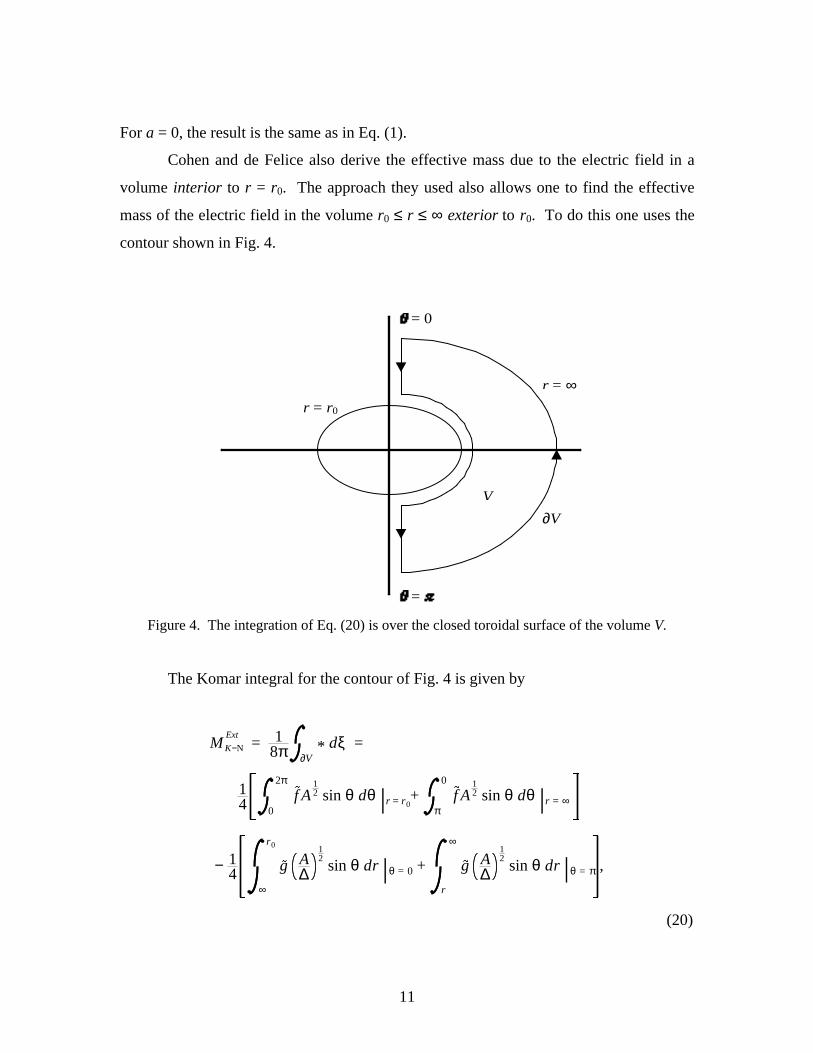
Cohen and de Felice also derive the effective mass due to the electric field in a

volume interior to r = r0. The approach they used also allows one to find the effective

mass of the electric field in the volume r0 ≤ r ≤ ∞ exterior to r0. To do this one uses the

contour shown in Fig. 4.

Figure 4. The integration of Eq. (20) is over the closed toroidal surface of the volume V.

The Komar integral for the contour of Fig. 4 is given by

M K−N

Ext= 1

8π * dξ∂V

=

14

f A12 sin θ dθ

0

2π

|r = r0+ f A

12 sin θ dθ

π

0

|r = ∞

− 14 g A

∆

12

sin θ dr

∞

r0

|θ = 0 + g A∆

12

sin θ dr

r

∞

|θ = π ,

(20)

r = r0

r = ∞

= 0

=

V

∂V

12

where,

g = aΩ A3

Σ 6∆

12

sin 2θ 1 + r2 + a2

a Ω .

(21)

In doing the integration, one must also take into account the path of integration

and the fact that for the volume V the normal to the surface r = r0 points in the negative

r-direction (opposite to the direction when computing the effective mass within this

surface). The last two integrals in Eq. (20) vanish, and the first two combine to both

eliminate the mass term associated with the ring singularity (which is exterior to the

volume of integration) and yield

M K−N

Ext=

Q2

2r0+

Q2

r02 + a2

2ar02 tan

−1 ar0

.

(22)

Thus, as in the case for the Reissner-Nordström solution, one has

M K−N

Int+ M K−N

Ext= m,

(23)

where m is the Schwarzschild or ADM mass.

Summary

By excluding the effects of rotation in the definition of effective mass for the

Kerr-Newman metric, it has been shown that the “negative mass” due to charge has

properties very similar to that of the Reissner-Nordström metric. Both take the

Minkowski form at r = Q2/2m, even though the meaning of r is different for the two

metrics; the effective mass interior to this surface is –m in both cases; and both have an

13

effective mass of m at infinity. In addition, the effective mass for both metrics satisfies,

for any surface defined by r = constant (again for either definition of r), the relation

M Eff

Int+ M Eff

Ext= m.

(24)

Thus the positive effective mass of the electric field exterior to the surface exactly

compensates for the “negative mass” associated with the charge located within the

surface.

Acknowledgement

The author would like to thank one of the referees for catching two typographical errors

and pointing out an interesting and relevant paper.

14

REFERENCES

[1] Marsh, G. E.: Charge, Geometry, and Effective Mass. Found. Phys. 38, 293-300(2008). In Eqs. (24) of this paper, the denominators on the r.h.s. should be R2.[2] Cohen, J. M. and de Felice, F.: The total effective mass of the Kerr-Newman metric.J. Math. Phys. 25, 992-994 (1984).[3] Kulkarni, R., Chellathurai, V., and Dadhich, N.: The effective mass of the Kerrspacetime. Class. Quantum Grav. 5, 1443-1445 (1988).[4] Chellathurai, V. and Dadhich, N.: Effective mass of a rotating black hole in amagnetic field. Class. Quantum Grav. 7, 361-370 (1990).[5] Komar, A.: Covariant Conservation Laws in General Relativity. Phys. Rev. 113, 934-936 (1959).[6] de Felice, F. and Bradley, M.: Rotational anisotropy and repulsive effects in the Kerrmetric. Class. Quantum Grav. 5, 1577-1585 (1988).[7] Henry, R. C.: Kretschmann scalar for a Kerr-Newman Black Hole. Astrophys. J 535,350-353 (2000).[8] An excellent discussion of these coordinates and their interpretation can be found in:Boyer, R. H. and Lindquist, R. W.: Maximal Analytic Extension of the Kerr Metric. J.Math. Phys. 8, 265-281 (1967).[9] Marsh, G. E.: The infinite red-shift surfaces of the Kerr and Kerr-Newman solutionsof the Einstein field equations. http://arxiv.org/abs/gr-qc/0702114. (2007)[10] de Felice, F. and Clarke, C. J. S.: Relativity on curved manifolds (CambridgeUniversity Press, Cambridge 1992).[11] Kulkarni, R. and Dadhich, N.: Surface geometry of a rotating black hole in amagnetic field. Phys. Rev. D 33, 2780-2787 (1986).[12] Cohen, J. M. and Moses, H. E.: New Test of the Synchronization Procedure inNoninertial Systems. Phys. Rev. Lett. 39, 1641-1643 (1977).