Brigham Young University Brigham Young University

BYU ScholarsArchive BYU ScholarsArchive

Theses and Dissertations

2015-12-01

Characterizing the Effects of Capillary Flow During Liquid Characterizing the Effects of Capillary Flow During Liquid

Composite Molding Composite Molding

Michael Ray Morgan Brigham Young University - Provo

Follow this and additional works at: https://scholarsarchive.byu.edu/etd

Part of the Industrial Technology Commons

BYU ScholarsArchive Citation BYU ScholarsArchive Citation Morgan, Michael Ray, "Characterizing the Effects of Capillary Flow During Liquid Composite Molding" (2015). Theses and Dissertations. 5787. https://scholarsarchive.byu.edu/etd/5787

This Thesis is brought to you for free and open access by BYU ScholarsArchive. It has been accepted for inclusion in Theses and Dissertations by an authorized administrator of BYU ScholarsArchive. For more information, please contact scholarsarchive@byu.edu, ellen_amatangelo@byu.edu.

Characterizing the Effects of Capillary Flow

During Liquid Composite Molding

Michael Ray Morgan

A thesis submitted to the faculty of Brigham Young University

in partial fulfillment of the requirements for the degree of

Master of Science

Andrew R. George, Chair Michael P. Miles

David T. Fullwood

School of Technology

Brigham Young University

December 2015

Copyright © 2015 Michael Ray Morgan

All Rights Reserved

ABSTRACT

Characterizing the Effects of Capillary Flow

During Liquid Composite Molding

Michael Ray Morgan School of Technology, BYU

Master of Science

As the aerospace industry continues to incorporate composites into its aircraft, there will be a need for alternative solutions to the current autoclaving process. Liquid composite molding (LCM) has proven to be a promising alternative, producing parts at faster rates and reduced costs while retaining aerospace grade quality.

The most important factor of LCM is controlling the resin flow throughout the fiber

reinforcement during infusion, as incomplete filling of fibers is a major quality issue as it results in dry spots or voids. Void formation occurs at the resin flow front due to competition between viscous forces and capillary pressure. The purpose of this work is to characterize capillary pressure in vacuum infusion, and develop a model that can be incorporated into flow simulation.

In all tests performed capillary pressure was always higher for the carbon fiber versus

fiberglass samples. This is due to the increased fiber packing associated with the carbon fabric. As the fabric samples were compressed to achieve specific fiber volumes an increase in capillary pressure was observed due to the decrease in porosity. Measured values for capillary pressure in the carbon fabric were ~2 kPa, thus the relative effects of Pcap may become significant in flow modeling under certain slow flow conditions in composite processing.

Keywords: capillary pressure, liquid composite molding, vacuum infusion, carbon fiber, resin infusion

ACKNOWLEDGEMENTS

I would like to express my gratitude and appreciation to Dr. Andrew George for the

constant encouragement and assistance during the course of this research. His enthusiasm and

vision for the future of composite processing was a motivating force for the completion of this

work.

Mention is made to my fellow classmate and colleague, Paul Hannibal, whose research

aided in the analysis and results of this work.

Love and appreciation to my wife Emily, for her constant support, patience, and sacrifice

through out this experience. Also to my parents, siblings, and friends who took interest in my

work and provided help and advice when needed.

iv

TABLE OF CONTENTS

LIST OF FIGURES ..................................................................................................................... vi

1 Introduction ............................................................................................................................. 1

1.1 Composite Incorporation and Purpose ............................................................................. 2

1.1.1 Economical Benefits and Environmental Goals ......................................................... 4

1.2 Manufacturing Processes.................................................................................................. 5

1.2.1 Autoclave Processing .................................................................................................. 5

1.2.2 Out-of-Autoclave (OoA) Processing .......................................................................... 6

1.2.3 Liquid Composite Molding (LCM) ............................................................................ 6

1.3 Simulation Modeling ........................................................................................................ 7

1.4 Problem Statement ........................................................................................................... 9

1.5 Hypotheses ....................................................................................................................... 9

2 Literature Review ................................................................................................................. 10

2.1 Capillary Pressure Measurement Methods ..................................................................... 12

2.2 Modeling Capillary Pressure .......................................................................................... 15

3 Methodology .......................................................................................................................... 18

3.1 Fabric .............................................................................................................................. 18

3.2 Test Fluid........................................................................................................................ 18

3.3 Experimental Design ...................................................................................................... 19

3.3.1 Fabric Dip Tests ........................................................................................................ 19

3.3.2 DIC/DAQ Vacuum-Bag Infusions ............................................................................ 21

4 Research Results and Analysis ............................................................................................ 24

4.1 Fabric Dip Tests ............................................................................................................. 24

4.1.1 Height vs. Time Data Acquisition ............................................................................ 24

4.1.2 Capillary Pressure Calculation Methods ................................................................... 26

v

4.1.2.1 Method A – Neglecting Gravity ....................................................................... 26

4.1.2.2 Method B – Partially Accounting for Gravity .................................................. 28

4.1.2.3 Method C – Fully Accounting for Gravity ....................................................... 29

4.1.3 Uncompressed Dip Test Pcap Results ........................................................................ 30

4.1.4 Compressed Dip Test Pcap Results ............................................................................ 36

4.1.5 Comparison of Pcap Results with Prediction ............................................................. 42

4.2 DIC/DAQ Infusion Results ............................................................................................ 45

4.2.1 Permeability Determination ...................................................................................... 45

4.2.1.1 Fiberglass Permeability ..................................................................................... 45

4.2.1.2 Carbon Permeability ......................................................................................... 47

4.2.2 Comparison of Compressibility for Infusion and Squeeze-flow .............................. 49

4.2.3 Pressure Gradient Comparison ................................................................................. 50

4.3 Pcap Comparison Between Dip Tests and DIC/DAQ Testing ........................................ 55

5 Conclusions ............................................................................................................................ 57

5.1 Future Recommendations ............................................................................................... 58

REFERENCES ............................................................................................................................ 59

vi

LIST OF FIGURES

Figure 1-1: Pictorial Representation of Materials Used on the Boeing 787 Dreamliner ................ 3

Figure 3-1: Vectorply Carbon Fiber (left) and JB Martin Fiberglass (right) Samples ................. 18

Figure 3-2: Experimental Setup for Compressed Fabric Dip Tests .............................................. 21

Figure 3-3: DIC/DAQ Test Plate Drawing ................................................................................... 22

Figure 3-4: Experimental Setup of DIC/DAQ System ................................................................. 23

Figure 4-1: Partially Saturated Carbon Fiber (Left) and Fiberglass (Right) Fabrics .................... 24

Figure 4-2: Flow Front Advancement in Carbon Fiber at 5, 20, and 50 Minutes ........................ 25

Figure 4-3: Original and Binary Image of Saturated Samples ...................................................... 26

Figure 4-4: h2 vs. t Average Profiles for Uncompressed Dip Tests .............................................. 31

Figure 4-5: Uncompressed Pcap Results for Method A: Each Sample (top); Averaged by Orientation (bottom) ............................................................................................. 32

Figure 4-6: Uncompressed Pcap Results for Method B: Each Sample (top); Averaged by Orientation (bottom) ............................................................................................. 33

Figure 4-7: Uncompressed Method C Plots for Determination of Average Pcap: Carbon (top), Fiberglass (bottom) ............................................................................. 34

Figure 4-8: Average Pcap Values for Uncompressed Flow Tests .................................................. 36

Figure 4-9: h2 vs. t Average Profiles for Compressed Dip Tests: Carbon (left), Fiberglass (right) ....................................................................................................... 37

Figure 4-10: Linear Fits for Only First Few Data Points from Figure 4-9 ................................... 38

Figure 4-11: Compressed Pcap Results for Method A: Carbon (left), Fiberglass (right); Individual (top), Averaged (bottom) ........................................................................ 39

Figure 4-12: Compressed Pcap Results for Method B: Carbon (left), Fiberglass (right); Individual (top), Averaged (bottom). ...................................................................... 40

Figure 4-13: Compressed Method C Plots for Determination of Average Pcap: Carbon (top), Fiberglass (bottom)............................................................................ 41

Figure 4-14: Average Pcap Values Throughout a Compressed Flow Test .................................... 42

vii

Figure 4-15: Fabric Compressibility Measurement Results from DIC/DAQ Testing for Fiberglass Infusion 2 and 3 ............................................................................... 46

Figure 4-16: Permeability as a Function of Fiber Content, Fit to Infusion Data, for Fiberglass DIC/DAQ Infusions................................................................................ 47

Figure 4-17: Compressibility Measured from Hannibal (2015) for Carbon Reinforcement .......................................................................................................... 48

Figure 4-18: Permeability as a Function of Fiber Content Fit to Infusion Data ........................... 48

Figure 4-19: Compressibility Determined by Instron During Squeeze Flow and by DIC/DAQ During Vacuum Infusion ........................................................................ 50

Figure 4-20: Inferred Pressure Gradient Results (George 2011) .................................................. 51

Figure 4-21: Experimental and Simulated Resin Pressure Gradient from Inlet to Flow Front for Carbon-3 DIC Infusion .................................................................... 53

Figure 4-22: Experimental and Simulated Data of PR gradient .................................................... 56

1

1 INTRODUCTION

Over the past decade civil aerospace manufacturers have made incredible technological

advancements with the incorporation of composite materials into their private and commercial

airplanes. The replacement of metal components by advanced composites has provided many

advantages and allowed for a lighter, more fuel-efficient aircraft. As industry continues to realize

the advantages of composite materials, it is continually searching for alternate solutions to the

current cumbersome manufacturing methods. Liquid composite molding (LCM) has proven to

be a promising alternative, producing parts at faster rates and reduced costs while retaining

aerospace grade quality.

The most important factor of LCM is controlling the resin flow throughout the fiber

reinforcement during infusion. Incomplete filling of fibers is a major quality issue as it results in

dry spots or voids, consequently decreasing the mechanical properties of the part. Simulation

software has been developed to better understand resin flow of different resin/fiber combinations

in an effort to improve mold design and eliminate void formation. Current simulation software

has limited accuracy when applied to particular processes due to inadequacies in addressing

capillary pressure.

Capillary pressure, also known as “wicking,” is the ability of a liquid to flow in narrow

spaces without the assistance of, and in opposition to external forces like gravity. During resin

infusion (RI), capillary pressure allows fiber bundles (tows or roving) to absorb resin until

2

complete saturation of the fiber bundle is achieved. This phenomenon has typically been deemed

negligible in simulation due to the use of high infusion pressures or low fiber content materials

during infusion processes. However, as incorporation of LCM processes into the commercial

aerospace industry is accepted for high-performance and large structural parts, high fiber content

materials along with low pressures (vacuum only for large parts) are required, causing capillary

pressures to be a significant component in accurate simulations of resin flow.

1.1 Composite Incorporation and Purpose

The aerospace industry for nearly a century has relied on metals for the structural support and

skin of its airplanes. This began in 1915 with the Junker J1, the first all metal airplane, composed

of an age hardened aluminum alloy known as duralumin. As airplane design continued to

advance, so did the metals with which they were built. Exotic aluminum alloys were developed

to meet specific needs, along with the incorporation of hard metals such as stainless steels, nickel

alloys, and titanium. Integrating these metals into critical areas of the body, wings, and engines

has enabled aerospace manufacturers to design and produce aircraft ranging from supersonic

fighter jets to double-deck, wide bodied airliners. Though metal has and will continue to play a

critical role in airplane design, industry has turned to alternative materials such as advanced

composites to provide comparable properties with less weight.

Application of composites on civil airplanes began with the interior cabin of the Boeing

707. Fiberglass composite was used on detail components within the cabin totaling a mere two

percent of the structural weight. Since the 707, both Boeing and Airbus have increased the use

of composites in their commercial airplanes as knowledge and manufacturability of composites

have improved.

3

In 2005 Airbus debuted the A380 utilizing composites extensively in the wings, tail

section, fuselage undercarriage, and doors. The A380 was also the first commercial airplane to

have a central torsion box made of carbon fiber reinforced plastic (CFRP). The sum of the

composites used on the A380 totaled 25 percent of the structural weight. Four years later Boeing

announced the 787 Dreamliner, which has composites comprising 50 percent of the structural

weight as shown in Figure 1-1 (Boeing 787 Dreamliner Specs 2015). It was the first commercial

aircraft to use CFRP extensively on both the skin and structure of the fuselage. In 2016 it is

projected for the Airbus A350 to hit the market and will surpass the 787 in overall composite use.

Just like the 787 its fuselage skin and structure will be composed of composites totaling more

than 53 percent of the structural weight. These airplanes represent the commercial sector’s

ingenuity and innovation to achieve both economical benefits and environmental goals.

Figure 1-1: Pictorial Representation of Materials Used on the Boeing 787 Dreamliner

4

1.1.1 Economical Benefits and Environmental Goals

Financial savings that are realized through the application of composites materials are

attributed to their net-shape capabilities, mechanical and chemical properties, and overall weight

reduction. Composite parts are constructed from layers of carbon fabric molded within a resin

matrix into a net shape, eliminating almost all scrap material. This is completely opposite from

metal parts which are typically cut from a block, forging, or casting, resulting in immediate loss

in material costs due to metal removal.

Mechanical and chemical properties of composites are also very beneficial financially.

Benefits such as increased strength, superior durability, and corrosion resistance, has allowed for

reduced maintenance costs and service inspections. On the Airbus A350, the service intervals

have been reduced from 6 years to 12, which significantly reduced maintenance costs for

customers (Innovative Materials 2015).

The largest financial impact, particularly in the long term, is reducing fuel consumption.

This is achieved by reducing the overall weight of the airplane. Composites materials are

typically 20 percent lighter than aluminum allowing manufacturers to maximize weight

reduction. This is a substantial savings on planes such as the 787 and A350 when considering

that over 50 percent of the structural weight is composite.

Reduced fuel consumption is not only economically- but also environmentally- friendly.

It is helping to further reach the goals that the Advisory Council for Aviation Research and

Innovation in Europe (ACARE) had in their 2001 report “European Aeronautics: A Vision for

2020” (Argüelles 2001). In the report’s environmental section it asked for there to be a total

engagement by the industry in a task of studying and minimizing the industry’s impact on the

global environment with 3 major goals outlined:

5

1. A reduction in perceived noise to one half of the current average levels.

2. A 50% cut in CO2 emissions per passenger kilometer (which means a 50% cut in fuel

consumption in the new aircraft of 2020)

3. An 80% cut in nitrogen oxide (NOx) emissions.

1.2 Manufacturing Processes

Processing of aerospace grade composite has two main requirements; one is minimal void

content, second being high fiber content of around 60 percent. Achieving both these

requirements maximizes the mechanical properties of the fiber/resin combination, while

minimizing weight. The most commonly used and reliable method to meet these requirements is

autoclave processing. Though reliable, autoclaves have their drawback such as high operating

costs and batch processing. This is why industry is actively pursuing the development of out-of-

autoclave processing that can meet quality requirements in order to reduce costs and increase

efficiency. LCM has been proven to be able to achieve both minimal void content along with

high fiber content.

1.2.1 Autoclave Processing

Autoclave processing utilizes pre-impregnated (pre-preg) fibers along with high pressure

to aid in complete wet out and high fiber content. Pre-preg fibers come in different forms, such

as unidirectional fiber rolls or woven mats, allowing for the layup process to be performed by

hand or automation. Fibers are applied to the mold in a designed layered pattern to apply

stiffness and strength to specific features of the part. The part may go through several debulking

cycles in order to remove air between layers and increase fiber density. A final vacuum bagging

is applied to the part, and it is placed in the autoclave oven. A vacuum hose will remain

6

connected to the part, while the oven is brought up to temperature and pressure. As temperature

increases it begins to cure the resin and pressure helps to remove excess resin along with

increasing the adhesion between fiber layers.

Drawbacks to the autoclaving process involve both cost and efficiency. The autoclave

itself is a substantial capital investment, especially as the size of the part increases. High

operational costs are associated with the energy required to reach both temperature and pressure

during curing. Curing cycles limit production to batch processing which reduces the rate and

efficiency at which the parts can be produced. As demand for aerospace composite structures

increases, it could easily surpass the autoclave capacity that is currently available in industry.

1.2.2 Out-of-Autoclave (OoA) Processing

Out-of-autoclave manufacturing techniques are alternatives to the current high-pressure

autoclave process. Typically OoA is very similar to the traditional autoclave process; utilizing

pre-preg fibers consolidated under a vacuum bag, but as the name implies it is simply oven cured

versus using an autoclave. These OoA prepregs are designed with lower viscosity resins to

achieve similar consolidation and degassing of voids at lower pressures. There are other

techniques that have been developed such as liquid composite molding, which utilizes dry fibers

that are infused with resin, then oven cured.

1.2.3 Liquid Composite Molding (LCM)

Liquid composite molding is a family of processes that utilize either double sided molds,

or single sided mold with vacuum bag. Determined by the mold and process used, resin is forced

through the fibers using mechanical pressure, vacuum pressure, or a combination of the two.

These processes have been shown to be very reliable and cost effective at producing comparable

7

parts to autoclave qualities. Resin transfer molding (RTM) has been successfully proven to

produce aerospace grade quality parts with minimal void content, and high fiber contents. One of

the drawbacks to RTM is because of high infusion pressures, a double-sided mold is required,

reducing its cost effectiveness for large composite parts. A solution is the advancement of a

current process known as vacuum infusion (VI).

Vacuum infusion requires only a single sided mold, covered in vacuum bagging. Similar

to autoclave processing, air is completely evacuated from the layup, minimizing entrapped air

and compressing the fibers. Resin is then drawn through the fibers until complete saturation is

achieved. Additional steps such as bleed out and vacuum at the inlet for less thickness variation

may be performed for optimal properties before parts are placed in the oven for curing.

The main limitation of LCM processes and particularly VI is the comprehension and control of

the resin flow front during infusion. Unlike random fiber mats, engineered woven fabric mats

display dual scale flow during resin saturation. This is due to the macro flow that occurs between

fiber tows, and micro-flow occurring as individual fibers become saturated within the tows.

Different effects are observed during infusions involving high pressure, low pressures, and

different fiber/resin combinations. Simulation modeling has been developed to help overcome

these parameters, but is not completely accurate for all processes.

1.3 Simulation Modeling

Simulation software including PAM-RTM, Polyworx, and LIMS has been developed to

model resin flow during infusion processes. Modeling has aided in reducing both time and cost

on mold development, which was traditionally accomplished through the trial and error method.

Features such as inlets, vents, and outlet ports can be properly positioned within the software

8

before tooling is even created; reducing mold rework, and minimizing dry spots, voids, and race-

tracking.

A current issue with simulation modeling is accurately modeling the resin flow front due

to the limited knowledge of particular variables. One of these variables is the capillary pressure

that is involved in the pressure gradient. Most modeling has neglected capillary pressure

because of the nature of the two principle markets where flow simulation is used. For high-

volume, smaller geometry composites, manufacturers use a resin transfer molding (RTM) type

process, where high pressures are required to force resin through tightly packed fibers causing

capillary pressures to be insignificant in comparison to the applied pressure gradient. In contrast,

the marine/energy industry manufactures low-volume, large parts using VI with low fiber

contents, decreasing the capillary effect that can occur between fibers. The aerospace industry

will require a mixture of these two processing techniques over the next 20 years allowing for

quick processes to produce large composite primary structures with high fiber content. Focus has

been given to VI due to the fact that RTM is limited to the size of components that can be created

because larger parts require pressures that are unfeasible.

In all cases, the accuracy of flow simulation is also hindered by the understanding of

variables more significant than the capillary pressure, such as permeability. But flow simulation

is constantly improving and capillary pressure is an issue that needs to be addressed. Critical

issues that are dependent on capillary flow, such as void prediction, are becoming more prevalent

in the literature. By neglecting capillary pressure, simulation models will be limited to the

accuracy with which they can predict the resin flow rate and pattern. The purpose of this research

is to characterize the capillary pressure effects in vacuum infusion, resulting in a model for

capillary pressure that can be incorporated into flow simulation.

9

1.4 Problem Statement

Efforts have been made to model the VI process, but most have deemed capillary pressures

insignificant because of low fiber volumes and high filling rates. By neglecting capillary

pressure, simulation models will be limited to the accuracy with which they can predict the flow

rate and pattern of a fiber resin combination in 3-dimensional modeling. The purpose of this

research is to characterize the capillary pressure effects in vacuum infusion, resulting in a model

for capillary pressure that can be incorporated into flow simulation.

1.5 Hypotheses

Capillary pressures will have a significant effect on the flow velocity when using high fiber

content reinforcement and slow resin infusion. Incorporating this additional pressure into the

pressure gradient will allow reasonable predictions of flow rates in both rigid tooling and

vacuum infusions.

10

2 LITERATURE REVIEW

During RI the overall quality of parts produced is highly dependent on complete

saturation of fibers by the resin flow front. As the resin flow front progresses throughout the

fiber matrix there is the inherent risk of dry spots or voids forming, which have a detrimental

effect on the physical and mechanical properties of the part. Research and studies have been

conducted on resin flow to improve current simulation software and aid in the understanding and

improvement of RI processes.

Complete saturation of a fiber preform requires all empty spaces between the fibers to be

filled with resin, including the space between fiber tows and the spaces between each individual

fiber that makes up the tow (Simacek 2010). Due to the complex architecture of engineered

fabrics and the inherent variation of layup technique and processing methods, there is a

probability that there will be regions inside fiber tows or in between fiber tows that will be

devoid of resin. In Kuentzer’s research (Kuentzer 2007) they hypothesized that pores within the

tows take 4.5 times longer to fill than the regions between the fiber tows. This is related to the

dual scale flow that has been observed at the resin flow front, which is the leading cause of void

formation in RI processes.

Dual scale flow is caused by viscous forces around the fiber bundles (macroflow) and

capillary forces between the fibers in the bundles (microflow) occurring simultaneously

(Gourichon 2006). The competition of these two flows causes a large difference in the position

11

of the flow front leading to the potential of void formation (Chang 1997). In the case of a high

resin velocity, voids will form within fiber tows because flow in the channel between tows is

faster than in the tow because of the high permeability of the channel (Figure 2-1 b). For low

resin velocity, however, the capillary flow will dominate within tows and hence voids will form

in the channels between tows (Figure 2-1 a) (Patel 1996, Kang 2000). This interplay between the

flows at the macro and micro scale will dictate whether the final microstructure of the composite

part manufactured is devoid of dry spots and voids.

Figure 2-1: Macro and Micro Void Formation. Reprinted from LeBel (2014)

Void content within a composite part is considered as representative of the part’s

structural integrity. As the presence of voids increases there is a degenerate effect on mechanical

performances such as interlaminar shear strength, flexural strength and compressive strength

(Ruiz 2006). Minimal void content is required in aerospace applications, and as the content

12

increases, so does the risk or scrapping the part. Therefore, in order to avoid the creation of voids

in the composite part, it is critical to understand not only the flow behavior at the macro scale,

but also what the role of capillary effects is in micro-impregnating the porous network.

Simulation of resin infusion is based on measurement or calculation of the pressure

gradient; the flow velocity is directly proportional to that pressure gradient. Pcap has been shown

to affect that pressure gradient (Lai 1997, Ahn 1991), although little effort to couple Pcap to

filling simulation exists in literature (Section 2.2), and even less to experimentally validate any

Pcap -coupled filling simulation model. At low pressure conditions in RI such as during slower

resin velocity when the flow front is far from the inlet, the levels of Pcap that have been measured

in literature can exceed the mechanically applied pressure gradient, thus implying that flow

simulation would be much more accurate when accounting for capillary effects.

2.1 Capillary Pressure Measurement Methods

Different measurement methods have been used to determine the capillary pressure in fluid

saturation of carbon and fiberglass fibers. A common first step to understanding capillary forces

is measurement of the wicking behavior of the fluid, based on the Wilhelmy plate method, a test

designed to calculate the surface tension of a liquid by measuring the force acted on a vertically

immersed plate. The surface tension of a liquid may be considered one of the most important

parameters influencing resin impregnation, as is it plays a key role in determining the wettability

of reinforcing fibers by a resin matrix in composite processing. Related to the surface tension, is

the contact angle, which decreases with the surface tension of the liquid. As the contact angle

decreases, the wettability of the system is said to improve. This has been found to translate in to

13

larger capillary pressures, which produce a higher rate of liquid penetration into fiber bundles by

wicking flow (Lee 1988, Ahn 1991).

Lee (1988) used this principle when performing dynamic wettability measurements on

carbon and Teflon fibers immersed in silicone oil and epoxy resin. A single fiber was immersed

in the liquids and the surface tension and contact angle was calculated for each interaction. This

work showed that the dynamic fiber wettability measurements give direct information on the

interaction between the fiber and resin to be processed.

Batch et al (1996) also applied Wilhelmy’s principle when measuring capillary flow,

driven by capillary forces only, in longitudinal and transverse direction inside fiber bundles. The

saturation rate was measured by suspending a fiber filled tube and submersing the base into a

fluid. As the fluid penetrated the fiber the increase of weight could be observed. This work was

unique as the fiber was held within a glass tube, which could influence the capillary flow of the

liquid.

Ahn et al (1991) designed and constructed an apparatus capable of measuring

simultaneously the unsteady-state permeability and capillary pressure in a simulated composite

impregnation experiment. Thirty plies of plain woven carbon fiber fabric were placed within the

apparatus and resin was forced through the preform with a constant force. The experiments

showed that as porosity increased capillary pressures decreased. At low porosity a maximum

capillary pressure of 37 kPa was observed. This pressure value is significant compared to even

the highest pressure gradient achievable in vacuum infusion, 100 kPa at sea level; a change of 37

kPa in the applied pressure gradient would result in a 37% change in the filling velocity for this

case.

14

Patel and Lee (1996) used a centrifuge apparatus to measure capillary pressure-saturation

relationships. The sample fiber mat was completely saturated with the test liquid and subjected to

centrifugal force at various speeds of rotation. Centrifugal force tries to force the liquid out of the

sample, while capillary pressure tries to contain it in the sample. The study also demonstrated

that lower fiber reinforcement porosity results in higher capillary pressures, but reduces

permeability and thus the bulk flow rate. Thus there would be an optimum porosity at which the

spontaneous impregnation rates are the highest.

Amico (2000) performed two different capillary infiltration experiments. The first was

similar to Lee (1988) and Batch et al (1996) where a single fiber was partially immersed in the

wetting liquid, and as the liquid uptake occurred due to capillary pressures only, weight and

height readings of the column of liquid were continuously taken. The second experiment

performed was with the same device, but instead of a single yarn, a single layer of plain woven

glass fabric was used, and height measurements were taken during the infiltration.

Neacsu (2006) studied radial impregnation of fiber tows. The cylindrical fibrous sample

were created by wrapping glass fibers around a tube to thicknesses of 12.5-60 mm. Sensors were

strategically inserted from one to five locations to signal arrival time of liquid saturation. The top

and bottom of the fibers were sealed so liquid could only enter from the outside diameter and air

could escape through the tube. The experiments were then initiated by immersing the sample in a

bath of impregnating liquid.

Min Li (2010) performed two separate infusion experiments, the first being driven by

vacuum pressures, the second driven by compressed air pressure. The employed driving pressure

was sufficiently low, less than 60 kPa, so that capillary pressure effects could not be neglected.

In these experiments the unidirectional glass fiber bundles were tested at different fiber volume

15

fractions of 50%, 60%, and 70%. Capillary pressures were then extrapolated from the data

gathered from infusion experiments.

Lebel (2014) utilized capillary rise experiments similar to those performed in Amico

(2000). The setup was developed to monitor simultaneously the flow front position and the total

uptake mass by spontaneous imbibition during a 24 hour test. The fabric was held in a glass mold

as it was lowered into a fluorescent dyed fluid. The dye, illuminated by a black light, allowed for

visual tracking of the fluid as it saturated the glass fibers. In conjunction with digital images

taken of the fluid rise, an automated tracking of the capillary front was developed in Matlab. The

experimental methodology proposed in Lebel’s paper can be used to characterize the imbibition

properties of fiber tows and fabrics as well as penetrativity of thermosetting resins. Moreover, it

can be used to identify the window of optimal flow front velocity to reduce void formation. The

experiments performed in this paper are very similar to experiments carried out in this work and

will be discussed later (section 3.3.1).

Note that only one previous test method characterized carbon fabrics (Ahn 1991), despite

the fact that the lower porosity inherent in carbon reinforcements compared to glass should cause

higher capillary pressures. This is assumed to be due to the opacity of carbon – which makes it

more difficult to monitor fluid wetting of the fabric compared with fiberglass. This study aims to

help fill in the gap of capillary characterization for carbon fabrics, where that data is needed the

most.

2.2 Modeling Capillary Pressure

The modeling of capillary pressure has been applied in several different methods. Pillai

(1998) modeled delayed impregnation of fiber tows by the inclusion of a “sink” (negative source

16

term) in the equation of continuity for the flow in the inter-two regions. Slade (2001) also

characterized the unsaturated flow behavior of various mats using a constant sink term in a

continuity equation, along with identifying a dimensionless number called the sink effect index

ψ. The sink effect index characterizes the magnitude of liquid absorption by the tows and is a

function of the relative resistance to the flow in the tow and inter-tow regions, and the packing

density of the tows. Gourichon (2006) included a sink term in there modeling that represented

liquid absorption velocity per unit volume and added additional volumes in the form of 1D

elements in their simulation model.

A simpler method to model the effects of capillary pressure in resin flow is to modify the

measured or calculated pressure gradient by adding (1991 Ahn) or subtracting (1997 Lai) the

capillary pressure, depending on whether the capillary flow is faster or slower, respectively, than

the bulk macro flow. As the flowrate during infusion is proportional to the pressure gradient, the

changes due to the capillary pressure directly affect the flowrate.

Another method for accounting for capillary flow is through the capillary number Ca.

The capillary number is a ratio of the viscous force to the capillary force and is define as:

𝐶𝐶𝐶𝐶 = 𝜇𝜇𝜇𝜇𝛾𝛾 (2-1)

where µ is the resin viscosity, ν is the global (macroscopic) resin velocity, and γ is the surface

tension of the resin. A modified capillary number was also sometimes used defined as:

𝐶𝐶𝐶𝐶∗ = 𝜇𝜇𝜇𝜇𝛾𝛾𝛾𝛾𝛾𝛾𝛾𝛾𝛾𝛾 (2-2)

which included θ to account from the contact angle between the fiber and resin. The capillary

number has often been used in permeability measurements (Hattabi 2005, Min Li 2010) and void

17

prediction models (Kang 2000, Gourichon 2006, Ruiz 2006) as void content could be shown to

be a function of the capillary number.

18

3 METHODOLOGY

3.1 Fabric

Two types of fabric reinforcements were selected to evaluate the capillary pressures

during saturation (Figure 3-1). The fiberglass reinforcement is an unbalanced weave, JB Martin

TG-15-N (518 g/m2) with PPG rovings. The carbon fiber sample is a +45/-45 biaxial non-

crimped fabric (NCF), VectorPly C-BX 1800 (580 g/m2).

Figure 3-1: Vectorply Carbon Fiber (left) and JB Martin Fiberglass (right) Samples

3.2 Test Fluid

The selected test fluid was store bought canola oil. This was an inexpensive alternative to

resins and other chemicals while still providing comparable characteristics. The hydrocarbon-

19

polymer nature of canola oil results in similar fluid properties to an epoxy or polyester resin, e.g.

surface tension, viscosity at room temperature, contact angles on a given surface.

3.3 Experimental Design

3.3.1 Fabric Dip Tests

Fabric samples were cut in 50 mm x 60 mm rectangles in both the warp and weft

directions. This allowed enough fabric for mounting and immersion into the fluid, while

maintaining a 50x50 mm2 area of saturation. Other studies discussed using die cutting for

samples to maintain edge quality, but a straight edge and razor were used with acceptable results

as no significant shear or fabric damage were observed.

Fabric dip tests were performed in a black room held at a temperature of 20°C ± 2°C.

Images were visually aided by a 75-watt fluorescent black light bulb and captured with a Sony

Alpha DSLR camera equipped with a Sigma 50 mm f/2.8 EX DG macro lens. The fabric was

slowly lowered until a minimum of 5mm was immersed in the oil. A large, wide reservoir

approximately 90mm in diameter and 40mm deep held 237 ml of oil in order to minimize oil

level fluctuation as the oil is wicked up into the reinforcement during saturation. A timer was

started and images taken at specified intervals for an hour, or until complete saturation was

achieved. For measurement calculations a scale was placed next to the samples and captured in

each photo so during analysis a correlation between millimeters and pixels could be set.

An initial issue discovered during experiments was the difficulty to see the canola oil’s

progression through the fabrics in the fabric dip tests. Many different solutions were explored

including food coloring, ink, soap dye, oil stain, and red chili oil, but all had poor results. Both

food coloring and ink were immiscible in the oil. The soap dye, oil stain, and red chili oil were

20

miscible, but as the mixture progressed through the fabric the coloring slowly faded, as it

appeared the coloring was being filtered out. Other similar experimental designs have employed

fluorescent dyes to monitor saturation in fiberglass (Lebel 2014). Adding a few drops of

Universal AC UV Dye to the canola oil and implementing a black light, the progression could

easily be seen in both the fiberglass and carbon fiber samples. To the author’s knowledge, this is

the first known published use of fluorescent dyes with carbon reinforcements as carbon is

opaque, but the polymer stitching threads in this NCF allowed tracking of the flow-front.

Non-compressed dip tests were performed with a single ply fiberglass and carbon fiber

fabric. Three tests were performed in both the warp and weft direction and for each of the two

reinforcement types for a total of 12 tests. Images were taken of the fiberglass tests at an interval

of 5 minutes until complete saturation was achieved. The carbon fiber samples filled at a much

slower rate (lower permeability and higher uncompressed fiber content) resulting in images

being taken every 5 minutes for the first 30 minutes, then every 10 minutes for the last 30

minutes.

Compressed dip tests were performed with four ply’s of each fabric. The samples were

held between two 13mm thick sheets of acrylic that were clamped together at each of the four

corners (Figure 3-2). Spacers ran the vertical length of each side of the fabric and were adjusted

to a specific distance to create the desired fiber volume. Sealing putty was also applied along the

lengths of the fabric between it and the spacers to minimize race-tracking and allow for a more

homogeneous, one-dimensional flow direction (consistent saturation). The fiberglass tests were

performed in the warp and weft direction for 40, 45, and 50 percent fiber volume, while the

carbon fiber was performed in the warp and weft for 50, 55, and 60 percent fiber volume. The

fiber volume was determined by the following equation:

21

𝑣𝑣𝐹𝐹 = 𝑛𝑛𝐴𝐴𝑊𝑊𝑤𝑤𝜌𝜌𝐹𝐹

(3-1)

where vF, n, AW, w, and ρF represent the fiber volume percent, number of plies, areal weight of

the fabric, thickness, and density of the fibers, respectively. Each combination of fiber

orientation and fiber volume was performed three times for a total of 36 experiments.

Figure 3-2: Experimental Setup for Compressed Fabric Dip Tests

3.3.2 DIC/DAQ Vacuum-Bag Infusions

Vacuum-bag infusions were performed in order to observe flow behavior using a

combination of digital image correlation (DIC) and data acquisition (DAQ) systems. Infusions

were performed on both carbon fiber and fiberglass samples, cut to dimensions of 400 mm by

250 mm, stacked four ply’s thick, all ply’s being longest in the warp direction. A special plate

22

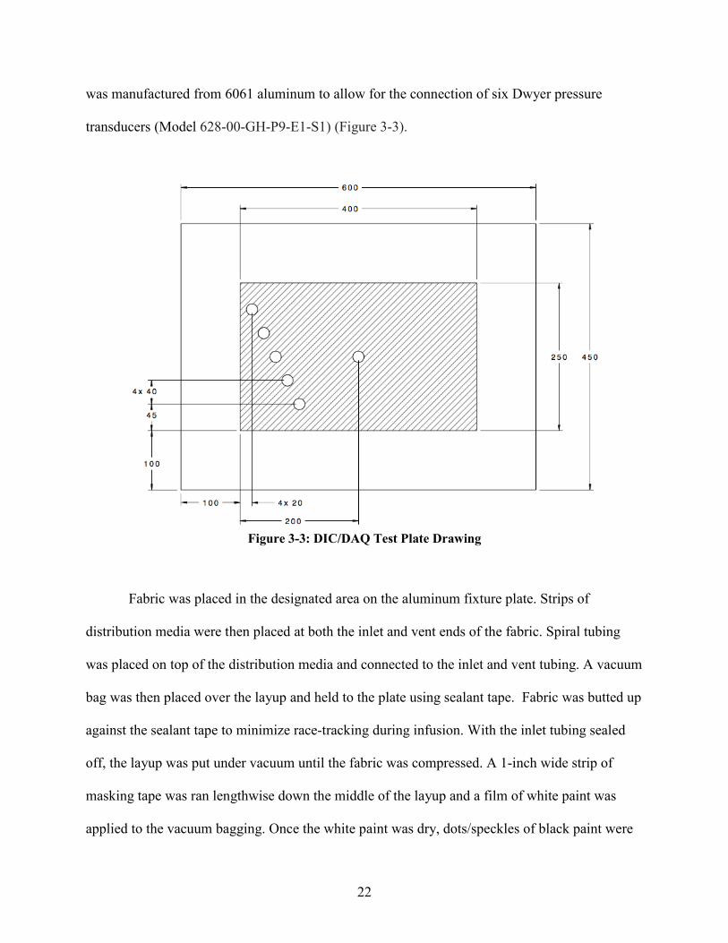
was manufactured from 6061 aluminum to allow for the connection of six Dwyer pressure

transducers (Model 628-00-GH-P9-E1-S1) (Figure 3-3).

Figure 3-3: DIC/DAQ Test Plate Drawing

Fabric was placed in the designated area on the aluminum fixture plate. Strips of

distribution media were then placed at both the inlet and vent ends of the fabric. Spiral tubing

was placed on top of the distribution media and connected to the inlet and vent tubing. A vacuum

bag was then placed over the layup and held to the plate using sealant tape. Fabric was butted up

against the sealant tape to minimize race-tracking during infusion. With the inlet tubing sealed

off, the layup was put under vacuum until the fabric was compressed. A 1-inch wide strip of

masking tape was ran lengthwise down the middle of the layup and a film of white paint was

applied to the vacuum bagging. Once the white paint was dry, dots/speckles of black paint were

23

applied over the white paint for contrast. The masking tape could then be removed so that resin

flow could be observed during the infusion in a thin strip along the flow direction (Figure 3-4).

Figure 3-4: Experimental Setup of DIC/DAQ System

With layup complete, it could then be placed under the DIC cameras and the transducers

were connected to the DAQ system. The inlet tubing was placed in an oil pot that was left open

to ambient pressure. The vent tubing was connected to a closed catch pot and brought to vacuum

pressure (0-10 mbar absolute pressure). A shim was placed on top of the layup to prevent caliper

indentation into the vacuum bag, and calipers were used to measure the thickness or height of the

fabric to use as a basis for calculating thicknesses from the DIC’s displacement data. After both

DIC and DAQ systems began collecting data, vacuum was removed and the fabric was allowed

to relax, so as to verify and calibrate the pressure readings from the measured DAQ electrical

signals. Vacuum was then reapplied to the layup, the inlet tube opened to the oil pot commencing

infusion, and the test was allowed to run until complete saturation of the fibers was achieved.

24

4 RESEARCH RESULTS AND ANALYSIS

4.1 Fabric Dip Tests

4.1.1 Height vs. Time Data Acquisition

With all fabric dip tests, both uncompressed and compressed, fluorescent dyed canola oil

was allowed to saturate up the fibers (Figure 4-1) until the flow front reached the top of the

sample. At various time intervals the height was measured to give a relation of height versus

time for oil saturation.

Figure 4-1: Partially Saturated Carbon Fiber (Left) and Fiberglass (Right) Fabrics

A similar test was presented in the literature (Amico 2000). This technique was

performed in a similar study (Lebel 2014) using fluorescent dye to visually track and measure

25

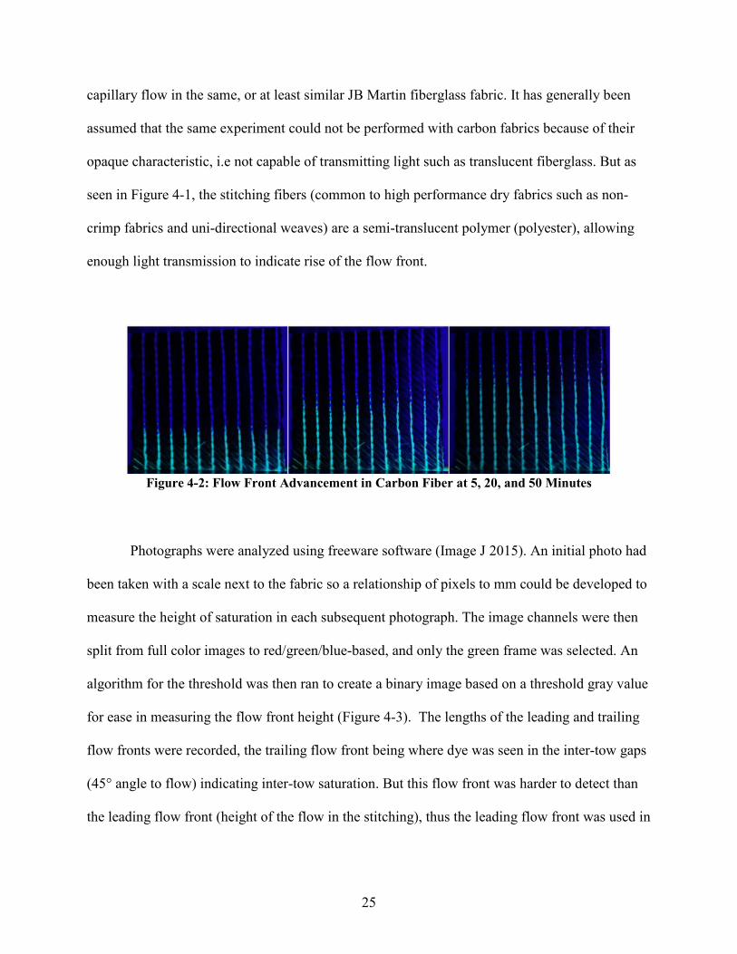
capillary flow in the same, or at least similar JB Martin fiberglass fabric. It has generally been

assumed that the same experiment could not be performed with carbon fabrics because of their

opaque characteristic, i.e not capable of transmitting light such as translucent fiberglass. But as

seen in Figure 4-1, the stitching fibers (common to high performance dry fabrics such as non-

crimp fabrics and uni-directional weaves) are a semi-translucent polymer (polyester), allowing

enough light transmission to indicate rise of the flow front.

Figure 4-2: Flow Front Advancement in Carbon Fiber at 5, 20, and 50 Minutes

Photographs were analyzed using freeware software (Image J 2015). An initial photo had

been taken with a scale next to the fabric so a relationship of pixels to mm could be developed to

measure the height of saturation in each subsequent photograph. The image channels were then

split from full color images to red/green/blue-based, and only the green frame was selected. An

algorithm for the threshold was then ran to create a binary image based on a threshold gray value

for ease in measuring the flow front height (Figure 4-3). The lengths of the leading and trailing

flow fronts were recorded, the trailing flow front being where dye was seen in the inter-tow gaps

(45° angle to flow) indicating inter-tow saturation. But this flow front was harder to detect than

the leading flow front (height of the flow in the stitching), thus the leading flow front was used in

26

further calculations. Although all example photos seen so far depict uncompressed tests, the

acquisition of height vs. time data in the compressed tests followed the same methodology.

Figure 4-3: Original and Binary Image of Saturated Samples

4.1.2 Capillary Pressure Calculation Methods

Three methods were used to infer the capillary pressure from the height vs. time data

measured in the dip tests.

4.1.2.1 Method A – Neglecting Gravity

Resin flow during composites processing has traditionally been modeled with Darcy’s

Law for porous media theory (Darcy, 1856). For one-dimensional flow neglecting the effects of

27

gravity, the velocity of flow can be integrated with respect to time to give the length versus time

relationship:

ℎ2

𝑡𝑡= 2𝐾𝐾𝐾𝐾𝐾𝐾

𝜑𝜑𝜑𝜑 (4-1)

Where h is length of flow going up through the height of the sample, t is time, K is permeability,

∆P is the change in pressure gradient, ϕ is porosity, and µ is the viscosity of the fluid. In a dip

test, the only pressure driving flow is the capillary pressure, thus Pcap can be substituted for ∆P

and then Pcap can be calculated from any data point of (h,t):

𝑃𝑃𝑐𝑐𝑐𝑐𝑐𝑐 = ℎ2𝜑𝜑𝜑𝜑2𝐾𝐾𝑡𝑡

(4-2)

Assuming known values for the porosity, viscosity and permeability. The permeability,

K, was experimentally determined, but the details will be presented later in this thesis along with

the tests used to determine it. The porosity was estimated as the non-compressed wet porosity,

which was also determined in experiments described later in this paper. The viscosity of the

canola oil test fluid was determined experimentally with a Brookfield viscometer at various

temperatures to build a model to predict the viscosity at any particular ambient temperature.

Equation 4-2 results in effective Pcap values at each of the data sampling time intervals.

Flow front progression is never very regular due to micro-variation in the textile (Vernet, 2014).

An averaged value for Pcap can be determined by fitting a linear equation to a plot of h2 vs. t,

where the slope, M equals:

𝑀𝑀 = 2𝐾𝐾𝐾𝐾𝑐𝑐𝑐𝑐𝑐𝑐𝜑𝜑𝜑𝜑

(4-3)

28

The slope is averaged across all data points, and thus the average Pcap across the

experiment can be determined by solving Equation 4-3 for Pcap. These forms of Darcy’s Law are

commonly used in experimental permeability determination (Vernet 2014).

4.1.2.2 Method B – Partially Accounting for Gravity

The second method for determination of Pcap only partially accounts for the effects of

gravity. The slope of h2 vs. t was again determined for each sample, assuming a linear profile

exists, which again neglects gravity. A function for the non-squared h(t) can be determined by

taking the square root of that linear fit, including the slope, M of that linear profile:

ℎ = √𝑀𝑀𝑀𝑀 (4-4)

Taking the derivative with respect to t gives us the inferred slope at any point:

𝑑𝑑ℎ𝑑𝑑𝑡𝑡

= 𝑀𝑀2

(𝑀𝑀𝑀𝑀)−1 2⁄ (4-5)

Equation 4-1 can be modified to incorporate the effects of gravity. Beginning with the non-

integrated velocity form of Darcy’s Law, and incorporating gravity as well as capillary pressure

as the only driver for flow (Amico 2000):

𝑑𝑑ℎ𝑑𝑑𝑡𝑡

= 𝐾𝐾𝜑𝜑𝜑𝜑

𝐾𝐾𝑐𝑐𝑐𝑐𝑐𝑐−𝜌𝜌𝜌𝜌ℎℎ

= 𝐾𝐾𝐾𝐾𝑐𝑐𝑐𝑐𝑐𝑐𝜑𝜑𝜑𝜑ℎ

− 𝐾𝐾𝜌𝜌𝜌𝜌𝜑𝜑𝜑𝜑

(4-6)

where K, µ, ϕ, Pcap, ρ, and g, are the permeability, viscosity, porosity, capillary pressure, liquid

density, and gravitational constant, respectively. The right-most term represents the contribution

of gravity, decreasing the flow rate dh/dt of the infusion. At short flow distances, the effects of

gravity are small, and the right-most term in Equation 4-2 can be disregarded, reverting back to

Equation 4-1. But in this calculation method, although the slope was determined assuming a

29

linear profile in h2 vs. t, that slope is used in Equation 6, leaving the gravity term in place.

Substituting Equation 4-5 (dh/dt) into Equation 4-6 and solving for Pcap:

𝑃𝑃𝛾𝛾𝐶𝐶𝑐𝑐 = ±ℎ� 𝑀𝑀𝜇𝜇𝑀𝑀2𝐾𝐾�𝑀𝑀𝑀𝑀

+𝜌𝜌𝜌𝜌� (4-7)

This function, given the height and time for a given data point, is Method B for determination of

Pcap.

4.1.2.3 Method C – Fully Accounting for Gravity

A solution was presented in Amico (2000) to determine Pcap from a dip test while fully

accounting for gravity. Equation 4-6 (Darcy’s Law with the gravity term) can be converted to a

linear equation:

𝑑𝑑ℎ𝑑𝑑𝑡𝑡

= 𝑀𝑀 1ℎ

+ 𝐵𝐵 (4-8)

where:

𝑀𝑀 = 𝐾𝐾𝐾𝐾𝑐𝑐𝑐𝑐𝑐𝑐𝜑𝜑𝜑𝜑

,𝐵𝐵 = −𝐾𝐾𝜌𝜌𝜌𝜌𝜑𝜑𝜑𝜑

(4-9)

This can lead to confusion, as M in this case is the slope (dh/dt vs 1/h) of a graph of data

including a different slope (h vs. t). The slope dh/dt in this case is not assumed linear but

approximated at each data point by taking the difference in height and time in succeeding

sampling steps. To minimize bias towards the initial fast flow, the instantaneous slope was

approximated by averaging the difference in heights and time for three successive measurement

points:

𝑑𝑑ℎ𝑑𝑑𝑡𝑡

= �ℎ2−ℎ1𝑡𝑡2−𝑡𝑡1

+ ℎ1−ℎ0𝑡𝑡1−𝑡𝑡0

�12 (4-10)

30

Each value of this slope is plotted against the corresponding value of 1/h, and the slope M

and intercept B can be fitted from the resulting graph as per Equation 4-8.

As the permeability is difficult to measure with certainty, the two parts of Equation 4-9

(for slope and intercept) were combined by solving each for K. The resulting combined equation

was then solved for Pcap:

𝑃𝑃𝑐𝑐𝑐𝑐𝑐𝑐 = −𝑀𝑀𝜌𝜌𝜌𝜌𝐵𝐵

(4-11)

This gives an average value for Pcap over the entire test range based on the fitted M and B

of the graph of 1/h vs. dh/dt.

4.1.3 Uncompressed Dip Test Pcap Results

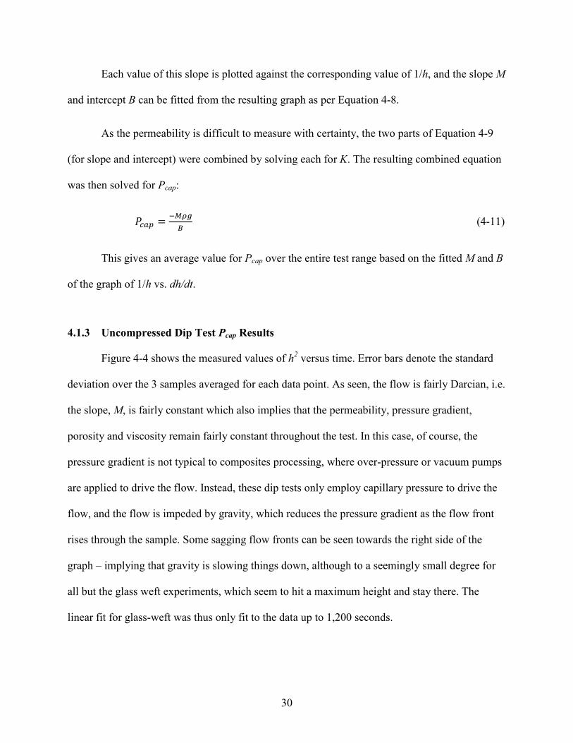
Figure 4-4 shows the measured values of h2 versus time. Error bars denote the standard

deviation over the 3 samples averaged for each data point. As seen, the flow is fairly Darcian, i.e.

the slope, M, is fairly constant which also implies that the permeability, pressure gradient,

porosity and viscosity remain fairly constant throughout the test. In this case, of course, the

pressure gradient is not typical to composites processing, where over-pressure or vacuum pumps

are applied to drive the flow. Instead, these dip tests only employ capillary pressure to drive the

flow, and the flow is impeded by gravity, which reduces the pressure gradient as the flow front

rises through the sample. Some sagging flow fronts can be seen towards the right side of the

graph – implying that gravity is slowing things down, although to a seemingly small degree for

all but the glass weft experiments, which seem to hit a maximum height and stay there. The

linear fit for glass-weft was thus only fit to the data up to 1,200 seconds.

31

Figure 4-4: h2 vs. t Average Profiles for Uncompressed Dip Tests

After calculating the Pcap for each time interval, the average Pcap value for each material

and orientation was plotted against h to observe the amount at which Pcap is changing as the flow

advances. This is shown in Figure 4-5 for Method A, Figure 4-6 for method B, and Figure 4-7

for method C.

Figure 4-5 shows linearly decreasing Pcap with flow height for all but one sample. This

decreasing trend is assumed to be due to the effects of gravity in that the flow rate is being

slowed down more and more by gravity as the test goes on, but the model to determine Pcap has

no way to account for that except to blame the decreasing flow rate on a decrease in the driving

pressure. The slope ranges from approximately 3 to 8 kPa/m for all of the four averaged plots.

The hydrostatic pressure head due to gravity is the product of the density, gravity and height, the

pressure divided by the height (slope) in Figure 4-5 should be approximately the product of

density and gravity, which in this case is about 9 kPa/m. This value is close to the range in

slopes, lending credibility to gravitational effects. Note that little difference exists between

orientations (warp vs. weft). Also, the carbon data shows about twice the capillary pressure as

32

glass, an understandable result due to the higher fiber packing in carbon compared to the glass

fabric.

Figure 4-5: Uncompressed Pcap Results for Method A: Each Sample (top); Averaged by Orientation (bottom)

Figure 4-6 (Method B) shows increasing slopes instead of decreasing slopes as were seen

in Figure 4-5 (Method A). This is probably due to the incongruence of not accounting for gravity

to determine dh/dt, and then using that value in an equation with a gravity term. The slopes in

this case are around 7-8 kPa/m for all but the glass weft averaged profiles, an even closer match

33

to the product of gravity and density as determined above. Note that in both cases, there is again

little difference between flow orientations, with error bars overlapping each other for the 0 and

90 degree tests. The agreement is especially clear for carbon in the averaged data, but even glass

has good agreement when looking at the individual tests. Carbon again results in higher Pcap than

glass.

Figure 4-6: Uncompressed Pcap Results for Method B: Each Sample (top); Averaged by Orientation (bottom)

34

Figure 4-7 (Method C) only shows results for the fitting of M and B to the data, for the

purposes of determination of the average capillary pressure by Equation 4-11. The fitted values

for M and B are seen on the charts. The initial data point (at the fastest flowrate) was neglected in

these fits as it was far from the rest of the data (up and too the right on this figure) and off the

linear fits from the other data points. The resulting profiles show fair linearity, justifying this

calculation method.

Figure 4-7: Uncompressed Method C Plots for Determination of Average Pcap: Carbon (top), Fiberglass (bottom)

The average Pcap value through each material and flow orientation was computed for

each test method, by using the average slope method described above for both Methods A and

35

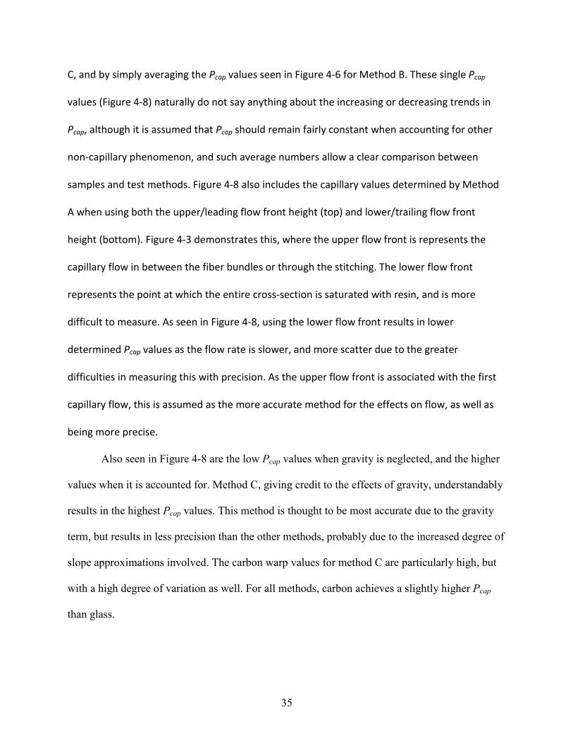
C, and by simply averaging the Pcap values seen in Figure 4-6 for Method B. These single Pcap

values (Figure 4-8) naturally do not say anything about the increasing or decreasing trends in

Pcap, although it is assumed that Pcap should remain fairly constant when accounting for other

non-capillary phenomenon, and such average numbers allow a clear comparison between

samples and test methods. Figure 4-8 also includes the capillary values determined by Method

A when using both the upper/leading flow front height (top) and lower/trailing flow front

height (bottom). Figure 4-3 demonstrates this, where the upper flow front is represents the

capillary flow in between the fiber bundles or through the stitching. The lower flow front

represents the point at which the entire cross-section is saturated with resin, and is more

difficult to measure. As seen in Figure 4-8, using the lower flow front results in lower

determined Pcap values as the flow rate is slower, and more scatter due to the greater

difficulties in measuring this with precision. As the upper flow front is associated with the first

capillary flow, this is assumed as the more accurate method for the effects on flow, as well as

being more precise.

Also seen in Figure 4-8 are the low Pcap values when gravity is neglected, and the higher

values when it is accounted for. Method C, giving credit to the effects of gravity, understandably

results in the highest Pcap values. This method is thought to be most accurate due to the gravity

term, but results in less precision than the other methods, probably due to the increased degree of

slope approximations involved. The carbon warp values for method C are particularly high, but

with a high degree of variation as well. For all methods, carbon achieves a slightly higher Pcap

than glass.

36

Figure 4-8: Average Pcap Values for Uncompressed Flow Tests

4.1.4 Compressed Dip Test Pcap Results

Figure 4-9 shows the h2 vs. t profiles for all material, orientation, and thickness

combinations. In contrast to Figure 4-4 (uncompressed tests), these profiles who definite sagging

in all cases, implying that gravity is playing a greater role at slowing the flow down as the

sample gets higher. The role of gravity is assumed to be playing a higher role here than in the

uncompressed test due to the slower flow / greater reduction in pressure caused by the greater

compaction. Thus the linear fits for Pcap determination by Method A were done using only the

data up through 1800 s for carbon, and 360 s for glass, to reduce the non-linearity caused by

gravity (Figure 4-10). Note that although the nonlinearity is reduced, there is still some sagging

in the right side of each profile even at these short times.

37

Figure 4-9: h2 vs. t Average Profiles for Compressed Dip Tests: Carbon (left), Fiberglass (right)

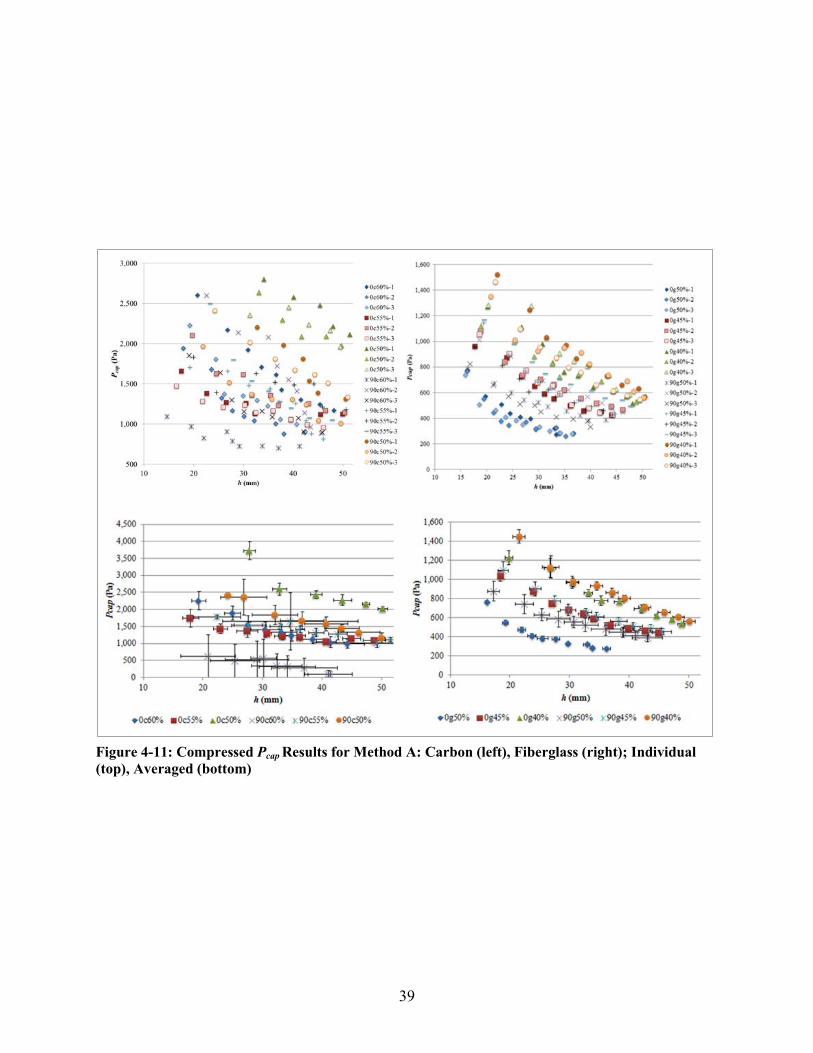
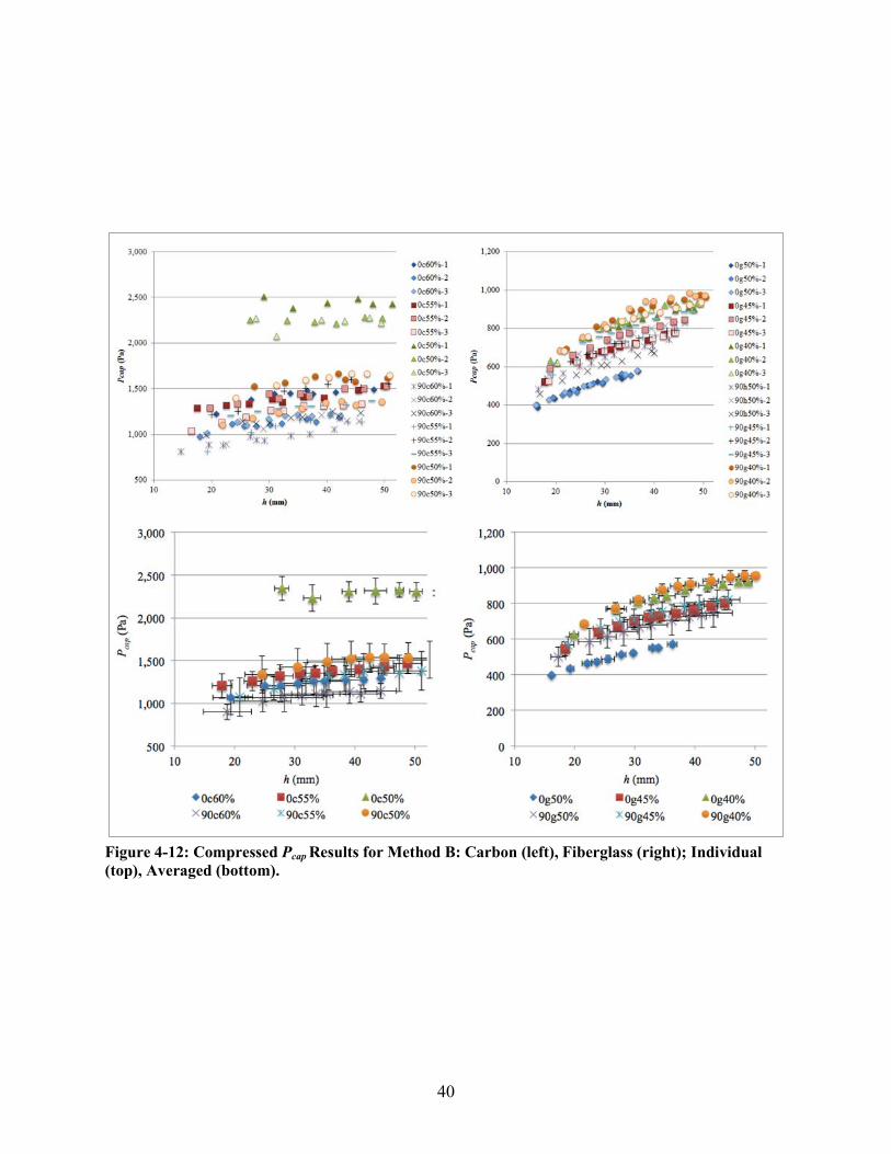
Figure 4-11 through 4-13 show the same graphs as Figure 4-5 through 4-7 but for the

compressed dip tests, including the three different thickness (compaction) levels. The figures

include first a graph of the individual plotted data points for each sample, and then a graph of

those data points averaged by orientation with errors bars representing standard deviation.

Method A (Figure 4-11) again shows decreasing slopes due to neglecting gravity in the flow

calculations. Method B (Figure 4-12) again reverses this trend and shows positive slopes. The

data in Method C (Figure 4-13) appears to be fairly linear again, thus validating this calculation

method.

38

Figure 4-10: Linear Fits for Only First Few Data Points from Figure 4-9

39

Figure 4-11: Compressed Pcap Results for Method A: Carbon (left), Fiberglass (right); Individual (top), Averaged (bottom)

40

Figure 4-12: Compressed Pcap Results for Method B: Carbon (left), Fiberglass (right); Individual (top), Averaged (bottom).

41

Figure 4-13: Compressed Method C Plots for Determination of Average Pcap: Carbon (top), Fiberglass (bottom)

Figure 4-14 shows the averaged values for each flow test again (as in Figure 4-8), this

time for the compressed tests. Carbon again shows higher Pcap than glass. In the uncompressed

results, Method A resulted in lower Pcap values than Method B, but no clear difference across all

fiber contents can be seen here in the compressed tests. Method C no longer provides the highest

estimates of Pcap, although a high standard deviation is again seen.

The results listed here for Pcap have been low (usually between 1 and 2 kPa) compared to

the 100 kPa provided by full vacuum at sea level in common infusion processing. During resin

42

infusion processing, however, that maximum pressure gradient of 100 kPa only exists when the

flow first enters the preform, and the pressure gradient at the flow front, driving the flow,

continues to diminish as the flow moves through the fibrous reinforcement. The maximum

pressure gradient is also reduced when infusing at higher altitudes than sea level. Thus the

relative effects of Pcap, even at 1 kPa may become significant in flow modeling under certain

slow flow conditions in composites processing.

Figure 4-14: Average Pcap Values Throughout a Compressed Flow Test

4.1.5 Comparison of Pcap Results with Prediction

A classic equation to describe capillary flow was derived (Ahn 1991) from capillary flow

modeling and adapted to flow in a fibrous reinforcement:

𝑃𝑃𝑐𝑐𝑐𝑐𝑐𝑐=𝐹𝐹𝐷𝐷𝑓𝑓∙ 1−𝜑𝜑

𝜑𝜑𝛾𝛾𝛾𝛾𝛾𝛾𝛾𝛾(𝛾𝛾𝐶𝐶𝐷𝐷) (4-12)

0

500

1,000

1,500

2,000

2,500

3,000

3,500

Atop-0 Atop-90 B-0 B-90 C-0 C-90

Pcap

(Pa)

glass 50% glass 45% glass 40%

carbon 60% carbon 55% carbon 50%

43

where F, Df, ϕ,θCD, are a form factor describing the flow direction in relation to the fiber

orientation, diameter of a single fiber, the surface tension of the liquid, and the dynamic contact

angle between the liquid and solid fiber surface, respectively. The difficulty with using this

equation is the difficulty in measuring the form factor and the dynamic contact angle. The latter

requires macro lens video of the capillary rise on a single 7-10 micron fiber as it is drawn out of

the liquid (Lee, 1996). But general comparisons can be made by relative estimates of these

variables.

In Equation 4-12, F is the form factor for alignment of the fibers to flow, being 4 for

along the fibers (parallel flow), and 2 for perpendicular flow. Both of these fabrics are nearly

isotropic in permeability (as discussed later in this paper). The carbon fabric is a balanced +45/-

45 biaxial fabric, with a very small stitching fiber being the only difference in flow orientation.

The fiberglass fabric is an unbalanced biaxial weave, but both warp and weft only differ a small

amount in areal weight. This is evident in the Pcap results, as there seems to be no difference in

flow orientation, implying that the form factor is fairly uniform for both warp and weft in both

materials. The porosity, surface tension, and fiber diameter are constant throughout a flow test.

The dynamic contact angle has been shown to slightly decrease as the velocity decreases (Lee,

1996), but the magnitude of this change on Pcap in Equation 4-12 is difficult to ascertain without

performing difficult measurements of θCD. Other possible sources of variation in the variables are:

1. In the uncompressed dip tests, the fluid flow is not completely 1D in the upward

direction, but flows off and down off the sides also.

2. Porosity may be changing with increasing lubrication, making a gradient in porosity

along the fabric from the fluid pool to the flow front.

44

If we neglect these two possible sources of variation, then Pcap should remain constant

throughout an experiment. Of course, methods A and B have shown to have regular gradients

one way or the other, which is assumed to be due to gravitational effects not being accounted for.

Compressed fabrics showed a higher Pcap than non-compressed. This is probably due to

the higher fiber volumes that were tested with the carbon fiber, which resulted in a higher

compression than the fiberglass tests, and would predict by Equation 4-12 a rise in Pcap along

with the decrease in porosity from higher compression.

For method A calculation, the Pcap values for carbon are a little less than twice that of the

fiberglass Pcap values (Figure 4-8). As these are both biaxial NCF’s, the form factor should be

similar. And the differences in flow rates are thought to cause minor differences in the dynamic

contact angle on similar sizing materials for both fiber types. The surface tension is equal in both

cases as it’s the same test fluid. Therefore the differences in fiber diameter (7 microns for carbon

and 10 for glass) and porosity (63% for carbon and 67% for glass) should account for the only

differences in Pcap according to Equation 12. With the variables for each fabric type, the

predicted Pcap from Equation 12 for carbon is 1.67 times that of glass, which agrees well with the

ratio seen in Figure 4-8 for method A. The lower porosity in carbon compared to glass is also

assumed to cause the rise in Pcap values seen in Figure 4-14.

In Figure 4.14, it can be noted that increasing porosity resulted in increasing Pcap for

methods A and B, while no significant trend can be seen in method C (all within each other’s’

standard deviation). This would seem to be a contradiction of Equation 12, as porosity is in the

denominator of the equation, and increasing porosity would increase the flow rate, and

correspondingly the contact angle, thus decreasing the cosine of the contact angle. These two

cases would both predict decreases in Pcap, not the increases seen in Figure 4.14. One possible

45

explanation would again be gravitational effects; gravity becomes more relatively important as

the flow slows down in more compressed samples. This may explain the lack of any clear trend

in Pcap for carbon using Method C, where gravity is accounted for, and no particular increase or

decrease is seen with increasing thickness.

4.2 DIC/DAQ Infusion Results

Along with the dip tests, two additional types of experiments were performed; one being

compressibility tests performed in another work (Hannibal, 2015), and the other were infusions

monitored by a DIC/DAQ system.

4.2.1 Permeability Determination

The fabric permeability, K that was used in later flow calculations was determined as

follows.

4.2.1.1 Fiberglass Permeability

The compressibility was taken from the DIC/DAQ infusion experiments that were

performed as part of this study. The compressibility is the function PC(vF) representing the

compaction pressure needed to achieve a given fiber content. This is analogous to a stress-strain

diagram in a compression test of any other material. The compressibility was determined as the

measured local fabric compression pressure (ambient pressure minus the local resin pressure as

measured by DAQ pressure transducers) for the measured sample fiber content (derived from the

sample thickness as measured with DIC). The compressibility data derived at the 20mm, 40mm,

and 60mm sensor points in fiberglass infusion number 2 and 3 (the others were regarded as

46

outliers) was averaged and then this data was fit to the Loos-Grimsley compressibility model

(Figure 4-17), which has previously shown good fitting for high vF fabrics (George 2011):

1 − �𝑣𝑣𝐹𝐹0𝐷𝐷𝑣𝑣𝐹𝐹� = 𝐴𝐴𝑤𝑤 + 𝐵𝐵𝑤𝑤 �

𝐾𝐾𝐶𝐶𝐶𝐶𝑤𝑤+ 𝐾𝐾𝐶𝐶

� (4-13)

Where Aw, Bw, and Cw are fitting constants. Aw represents a relationship between the dry

uncompressed fiber content (vf0D) and the wet uncompressed fiber content (vf0W), Aw = 1-

(vfoD/vf0W). The average compressibility was fit with the following constants: Aw = 0.0934, Bw =

0.364, and Cw = 44.43 mbar.

Figure 4-15: Fabric Compressibility Measurement Results from DIC/DAQ Testing for Fiberglass Infusion 2 and 3

This compressibility function was taken and put into a Matlab program that fits a

permeability function, K(vF) (the permeability at a given fiber content; a power law function K =

AK·vFBK) to the L versus t data as measured by monitoring flow front position through the

DIC/DAQ infusions. The Matlab model was developed as a version of Darcy’s law that accounts

for the change in thickness during vacuum infusion (under a vacuum bag) as described in (Modi

2009, Correia 2004). This model was modified from the usual calculation of filling time, to fit

47

the permeability to the filling rate. The permeability was fit in this way to the L vs. t data for all 5

DIC/DAQ fiberglass infusions (all in the warp direction), and resulted in five fits for AK and BK.

These were averaged (Figure 4-18) to result in the follow permeability fit constants: AK =

3.9·10-11 m2 and BK = -0.56.

Figure 4-16: Permeability as a Function of Fiber Content, Fit to Infusion Data, for Fiberglass DIC/DAQ Infusions

With no infusions performed in the weft direction, and the literature showing little

anisotropy in flow for this material (George 2014), the fabric was assumed to be isotropic, and

these warp values were used for the weft permeability as well. A literature value at a low fiber

volume (38.5%) was very high (7.8·10-10 m2) compared to extrapolation of this fitted model

which prompts the need for further testing to verify the assumption of anisotropic flow.

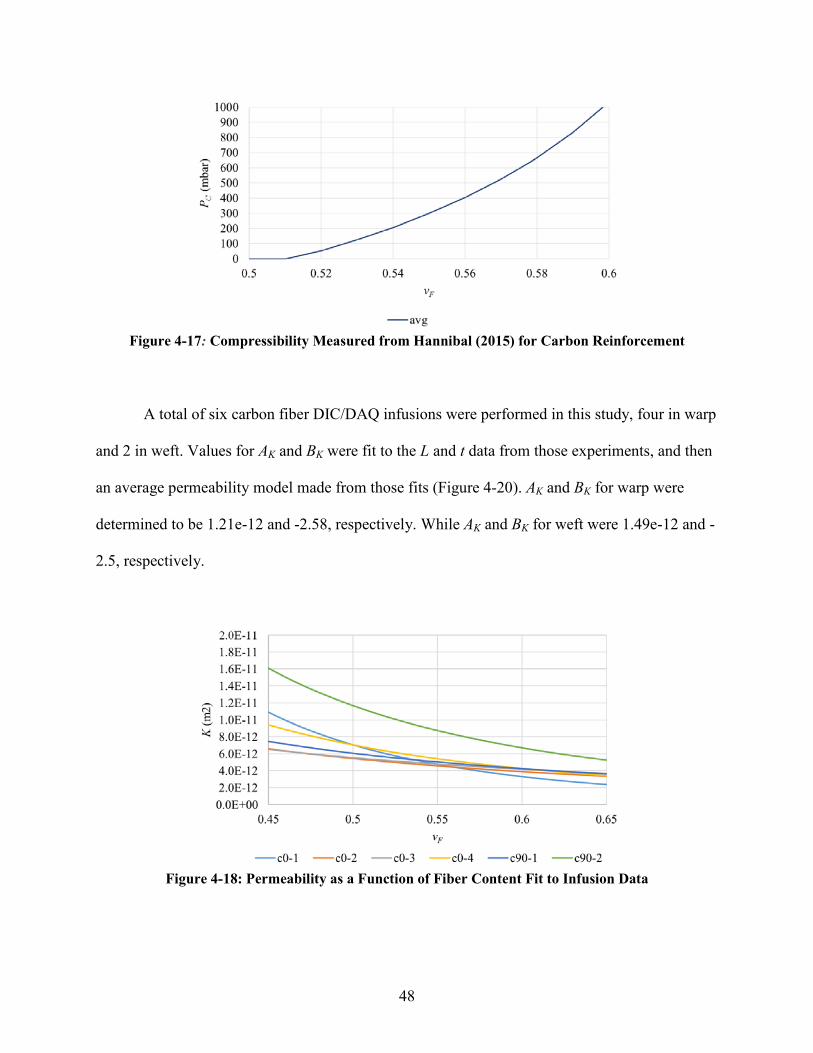
4.2.1.2 Carbon Permeability

For carbon, the compressibility model used (Figure 4-19) was a fit of Equation 4-13 to

averaged data from compressibility tests on 5 carbon fiber samples in canola oil performed

elsewhere (Hannibal 2015). The compressibility model used was: Aw = 0.3190, Bw = 0.1827 and

Cw = 853.5 mbar.

48

Figure 4-17: Compressibility Measured from Hannibal (2015) for Carbon Reinforcement

A total of six carbon fiber DIC/DAQ infusions were performed in this study, four in warp

and 2 in weft. Values for AK and BK were fit to the L and t data from those experiments, and then

an average permeability model made from those fits (Figure 4-20). AK and BK for warp were

determined to be 1.21e-12 and -2.58, respectively. While AK and BK for weft were 1.49e-12 and -

2.5, respectively.

Figure 4-18: Permeability as a Function of Fiber Content Fit to Infusion Data

49

4.2.2 Comparison of Compressibility for Infusion and Squeeze-flow

The DIC/DAQ tests were done with vacuum infusion, which involves wetting flow, with

Pcap affecting the filling rate as it changes the pressure gradient at the flow front. The

compressibility (Equation 4-13) was fit to the data at sampled time increments for the

compaction pressure right at each pressure transducer and the thickness of the preform for any

time at which the flow front had passed each transducer.

In contrast, the Instron-determined compressibility tests done in Hannibal (2015) = fabric

soaked in bath of oil or epoxy, squeezed under Instron in compression and then soaks up the

fluid again as the Instron retreats and the sample relaxes and grows in thickness. The load on the

Instron minus the calculated total resin pressure on the sample resulted in the compaction at any

time and sample thickness, giving the compressibility function shown in Figure 4-19. The

sample has to squeeze and expand, which includes the fiber bundles, so there’s capillary flow in

and out of the fiber bundles, but all the fibers should already be wetted which implies that Pcap

effects are small if any. Thus although the absolute capillary pressure involved is yet unknown

for both the DIC/DAQ tests in this study and the squeeze-flow tests done in Hannibal (2015), a

comparison of the resultant compressibility curves should allude to the differences in capillary

pressure effects. Figure 4-21 shows the average compressibility determined from all tests

involving the carbon NCF for both methods. Note that the squeeze-flow compressibility in

Figure 4-19 comes from the Instron load data during expansion of the wet fabric, which is

thought to be most accurate to infusion. But pressure sensor data in that study suggests that the

sample was not expanding as fast as the Instron cross-head, so the compression data during that

test might give better data. Thus the compressibility models from both expansion and

compression squeeze-flow data are shown in Figure 4-21.

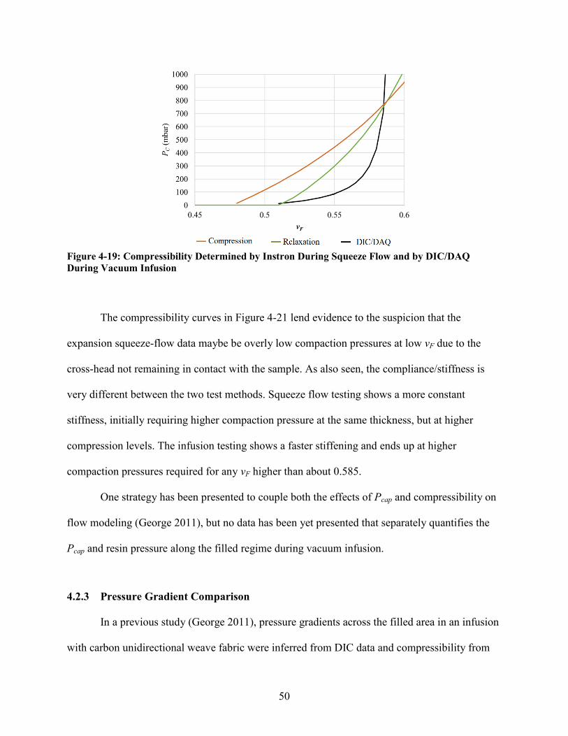
50

Figure 4-19: Compressibility Determined by Instron During Squeeze Flow and by DIC/DAQ During Vacuum Infusion

The compressibility curves in Figure 4-21 lend evidence to the suspicion that the

expansion squeeze-flow data maybe be overly low compaction pressures at low vF due to the

cross-head not remaining in contact with the sample. As also seen, the compliance/stiffness is

very different between the two test methods. Squeeze flow testing shows a more constant

stiffness, initially requiring higher compaction pressure at the same thickness, but at higher

compression levels. The infusion testing shows a faster stiffening and ends up at higher

compaction pressures required for any vF higher than about 0.585.

One strategy has been presented to couple both the effects of Pcap and compressibility on

flow modeling (George 2011), but no data has been yet presented that separately quantifies the

Pcap and resin pressure along the filled regime during vacuum infusion.

4.2.3 Pressure Gradient Comparison

In a previous study (George 2011), pressure gradients across the filled area in an infusion

with carbon unidirectional weave fabric were inferred from DIC data and compressibility from

51

squeeze flow in Instron testing(Figure 4-20). Results from that study are shown in Figure 4-22

for a carbon unidirectional weave, where the pressure gradient is presented as a function of α,

representing the relative position between the inlet side of the reinforcement (α = 0) and where

ever the flow front is (α = 1). Thus α = 0.5 implies a point halfway between the inlet and the flow

front, where ever that is as the flow continues to move through the sample during infusion. Note

that these values for the resin pressure were not measured directly, but “inferred” (calculated

indirectly) evaluating the equivalent resin pressure from the compressibility model from Instron-

testing for the measured thickness from DIC.

Figure 4-20: Inferred Pressure Gradient Results (George 2011)

In Figure 4-22, the solid black line is the pressure gradient as predicted by Darcy’s Law

where the fabric thickness does not change. The pressure should be a linear gradient from the

inlet pressure (ambient in the case of vacuum infusion) to the vacuum pressure on the vent. The

dashed line is the predicted pressure gradient from the Modi-Correia model (Modi 2008, Correia

52

2004) which accounts for the vacuum bag height change, and was calculated using the

compressibility determined from Instron-testing. The slope of the pressure gradient at the flow

front (α = 1) determines the filling speed at that moment during the infusion; the steeper the

negative slope, the faster the infusion. Vacuum infusion allows for more thickness by the resin

inlet, and thus less pressure loss there than a fixed height infusion, thus making the slope slightly

steeper and faster flow.

The dotted line in Figure 4-22 was a version of the Modi-Correia model, coupled to a

prediction of the contribution by capillary pressure based on the Ahn model in Equation 4-12.

This is based on the pressure balance:

𝑃𝑃𝑐𝑐𝑎𝑎𝑎𝑎𝑎𝑎𝑎𝑎𝑛𝑛𝑡𝑡 − 𝑃𝑃𝑣𝑣𝑐𝑐𝑐𝑐𝑣𝑣𝑣𝑣𝑎𝑎 + 𝑃𝑃𝑐𝑐𝑐𝑐𝑐𝑐 = 𝑃𝑃𝐶𝐶+𝑃𝑃𝑅𝑅 (4-14)

The colored data points in Figure 4-22 are the inferred resin pressures along the filled

area when the flow front was 20 mm along in filling the sample, 40, 70, 100, and 135 mm. Those

resin pressure dropped to negative “effective” pressures, much lower than the usually-assumed

vacuum pressures by the flow front. This suggested that the capillary pressure contribution in

Equation 4-14 may be much larger than the black dashed line model was predicting, and

suggesting that the contribution of Pcap to the overall flow rate may be much higher than

previously assumed. These conclusions led to the use of DIC/DAQ in this study to try to

reproduce these results, but with DAQ and pressure transducers to directly measure the resin

pressure to try to validate these capillary effects.

In more recent work (Hannibal 2015), it was shown that the compressibility models used

to determine the data in Figure 4-22 were faulty; the contribution of resin pressure to the load on

the Instron was not accounted for when calculating the compaction pressure on the

reinforcement.

53

In this study, the two compressibility models (from squeeze-flow and directly from the

DIC/DAQ data during infusion) were evaluated against each other by plugging each model into

the Modi-Correia model and comparing the resultant pressure gradients. Figure 4-21 shows the

modeled pressure gradients from the data and compressibility models for the third carbon DIC

infusion. Again, the linear Darcy’s law gradient, the Modi-Correiea model, and the model

coupled with an approximated Pcap are all shown. The actual measured resin pressures from the

pressure transducers are also included in the graph, arranged similar to Figure 4-22 where the

resin pressure across the filled regime is presented in different symbols, for when the flow front

is at various lengths corresponding to the position of the 6 pressure transducers. When the flow

front is at 20mm, there is only one pressure sensor (the one at 20 mm) measuring pressure at an

infused location, resulting in only one data point. When the flow front reaches 200 mm, all 6

sensors are measuring pressure at filled locations and more data points are shown.

Figure 4-21: Experimental and Simulated Resin Pressure Gradient from Inlet to Flow Front for Carbon-3 DIC Infusion

As seen in Figure 4-21, the measured values of PR “bow” up from the linear Darcy’s Law

model, as predicted by the Modi-Correia model. But neither compressibility model results in the

same amount of curvature as the measured values for PR, which are independent of Pcap. This

54

implies that these compressibility models are under-predicting the compliance (opposite of

stiffness) due to Pcap effects. As discussed in Section 4.2.2, the squeeze-flow tests should have

less Pcap involved then in the actual infusion. As the left graph represents the filling prediction

using the squeeze-flow compressibility model, it exhibits more compliance than the right graph’s

results based on infusion compressibility. This implies that when Pcap forces are involved in the

compressibility testing, and not accounted for, i.e. separated from the other pressures involved,

then the compressibility results in a lower compliance (stiffer model) than the true nature of the

reinforcement. But even the squeeze-flow compressibility model still under predicts the

compliance, suggesting that Pcap forces may still be somehow involved in that test, although to a

lesser extent than during infusion.

As the pressure gradient predictions in the right graph in Figure 4-21 are resultant from

compressibility based on full Pcap effects, and the measured PR points are independent of Pcap,

the difference between the two may be an approximation of the relative effect of Pcap on the flow

rate during infusion. The flow rate is proportional to the pressure gradient at the flow front (α =

0). The predicted pressure gradient with no coupled effects from Pcap ends up at α = 0 at the same

pressure as the measured pressure gradient (the vacuum pressure, 300 Pa), but seems to have a

slightly lower pressure gradient (less downward curvature), thus under-predicting the flow rate.

The flow model coupled with a Pcap term in the pressure balance (dotted line in Figure 4-21) has

a slightly steeper pressure gradient than the non-coupled model, and may be closer to the

experimental gradient at the flow-front, although it’s hard to tell without more data points around

the flow front and just behind it. But the difference between the experimental PR and the coupled

model at the flow-front is equal to the approximated value for Pcap used in the flow model, which

is based on Equation 4-12. Thus the difference is still simulated and not measured.

55

4.3 Pcap Comparison Between Dip Tests and DIC/DAQ Testing

Figure 4-22 shows the data from Figure 4-21 (left side – squeeze flow compressibility

model), with only experimental data for the pressure gradient when the flow-front is at the

transducer at 100 mm. Added to this graph is the “inferred” pressure gradient as was done in

Figure 4-22, where the thickness data across the entire 100 mm (sampled at high resolution in

DIC) was converted to their equivalent PR values by using the compressibility model determined

from infusion – in essence using the average relationship between DIC data and DAQ data for

that test. This allows one to see the entire PR gradient from the experiment instead of just a

couple points at the transducer locations. But as seen in Figure 4-22, this profile departs from the

experimental PR gradient. First, a “tail” is seen in the bottom right, where the inferred PR values

jumps up. This was noted previously (George 2011) and is the effect of measuring thicknesses

around the flow front where the reinforcement is only partially saturated, before either bulk flow

or Pcap effects finish saturating everything just behind the flow front. Partial saturation means the

reinforcement is partially dry, which makes the material stiffer due to less lubrication. The length

of this tail is thus related to the difference in speeds for capillary flow and bulk flow between the

fiber bundles. The compressibility model determination doesn’t reflect this partial saturation

because most of the transducer data sampling is done when the flow front is somewhere in

between the transducers, and very few data comes from when the partially saturated flow front is

right over a transducer.

The other departure from the experimental pressure gradient is the drop below the

experimental values, even to negative pressures before the partial lubrication tail brings it back

up. Although this is not as severe a drop as was seen in Figure 4-22 with a faulty compressibility

model, this is still evidence of negative effective pressures due to Pcap forces acting on the

56

pressures involved during infusion. The thickness under the vacuum bag is affected by both PR

and Pcap, thus the difference between this inferred profile and the PR experimental values is

assumed to be a relative experimental determination of the effects of Pcap. The precision of DIC

testing seems somewhat inadequate to measure the difference between this and the experimental

PR values with confidence (the negative PR values seem suspiciously low), especially not

knowing for sure at what point partial saturation is making the curve shoot up into unusable data.

But a difference of about 50 mbar (5 kPa) is a visually approximated difference between the 2

curves. The thickness of the sample by the flow front during this infusion was about 2.2 mm, and

this carbon infusion was done in the warp direction. Looking back at Figure 4-14, the warp Pcap

at this thickness (corresponding to 60% fiber content) was determined in the dip tests to be about

1.3 kPa, which is lower than the 5 kPa estimated from infusions, but is at least in the same order

of magnitude, and doesn’t look as bad of a match when considering all the sources of error from

DIC, DAQ, and compressibility fitting associated with the infusion Pcap measurement method.

Perhaps with better data sampling, and continued further testing, the relationship between Pcap

values determined in infusion and in dip testing will be made clearer.

Figure 4-22: Experimental and Simulated Data of PR gradient

57

5 CONCLUSIONS

Fabric dip tests were conducted similar to previous studies, using fluorescent dye to

visually track and measure capillary flow. The stitching fibers in a carbon NCF allowed enough

light transmission to indicate rise of the flow front. Three methods were used to infer the

capillary pressure from the height vs. time data measured in the dip tests: neglecting gravity,

partially accounting for gravity, and fully accounting for gravity. The latter method resulted in

the highest calculated values of capillary pressures, and is assumed to be the most accurate of the

measurement methods, although it was not as precise as the other methods. Values for Pcap were

measured by this method of ~2 kPa for the carbon fabric. Thus the relative effects of Pcap may

become significant in flow modeling under certain slow flow conditions in composites

processing.

Along with the dip tests, infusions were also monitored by a DIC/DAQ system.

Comparison of compressibility data from this experiment with the data from a squeeze-flow test

lends evidence to the suspicion that the expansion squeeze-flow data may be resulting in overly

low compaction pressures. Squeeze flow testing shows a more constant stiffness, while the

infusion testing shows a faster stiffening and ends up at higher compaction pressures required for

any vF higher than about 0.585.

The measured values of resin pressure in these infusion tests “bow” up from the linear

Darcy’s Law model, as predicted by the Modi-Correia model. The compressibility models used

58

results in less curvature than the measured values for resin pressure, which are independent of

Pcap. This implies that these compressibility models are under-predicting the compliance

(opposite of stiffness) due to Pcap effects, which are involved in compressibility testing. The flow

model coupled with a Pcap term in the pressure balance has a slightly steeper pressure gradient

than the non-coupled model, and seems to be closer to the experimental gradient at the flow-

front. The dip in the effective resin pressure (inferred from the thickness) to levels below the

vacuum pressure can be attributed to Pcap and this same dip is seen in the model.

5.1 Future Recommendations

For the improvement of future testing and analysis similar to that which has been

performed in this work, the following recommendations are given. Dip tests would be repeated,

but performed with different fluids to see if the change in contact angle and surface tension does

indeed alter the capillary pressure as predicted by Equation 4-12. Each fluid would also be tested

to measure the dynamic contact angle θCD, to improve the resulting Pcap in equation 4-12.

59

REFERENCES

Ahn, K. J., J. C. Seferis, and J. C. Berg. "Simultaneous measurements of permeability and capillary pressure of thermosetting matrices in woven fabric reinforcements." Polymer composites 12.3 (1991): 146-152.

Amico, S.C. Permeability and Capillary Pressure in the Infiltration of Fibrous Porous Media in Resin Transfer Moulding. University of Surrey, 2000

Argüelles, P., et al. "European Aeronautics: A vision for 2020." Advisory Council for Aeronautics Research in Europe, Report (2001).

Batch, G. L., Y.T. Chen, and C.W. Macoskot. "Capillary impregnation of aligned fibrous beds: experiments and model." Journal of reinforced plastics and composites 15.10 (1996): 1027-1051.

"Boeing 787 Dreamliner Specs." Modern Airliners. Web. 20 Nov. 2015.

Chang, C.Y., L.W. Hourng, and C.J.Wu. "Numerical study on the capillary effect of resin transfer molding." Journal of reinforced plastics and composites 16.6 (1997): 566-586.

Correia, N.A.C.M. Analysis of the vacuum infusion moulding process. PhD. diss. University of Nottingham, 2004.

Darcy, H.P.G. Les fontaines publiques de la ville deDijon. Paris: Dalmont (1856).

George, A., H. Ahlborn, M. ElGhareeb, K. Drechsler, and D. Heider. “Compressibility Modeling and Validation for Coupled Flow Simulation.” Paper presented at the 18th International Conference on Composite Materials (ICCM), Jeju, South Korea, 2011.

George, A. Optimization of resin infusion processing for composite materials: simulation and characterization strategies. Diss. University of Stuttgart, 2011.

George, A. “Rigid Tooling for Optical 3D Wetting Permeability Measurements” FPCM 12 Enschede, The Netherlands. 14 July 2014. Lecture.

Gourichon, B., C. Binetruy, and P. Krawczak. "A new numerical procedure to predict dynamic void content in liquid composite molding." Composites Part A: applied science and manufacturing 37.11 (2006): 1961-1969.

60

Hannibal, P. "Compressibility Measurement and Modeling to Optimize Flow Simulation of Vacuum Infusion Processing for Composite Materials." (2015).

Hattabi, M., et al. "Flow analysis during on-line and radial injection applications in permeability measurements." Journal of reinforced plastics and composites24.18 (2005): 1909-1920.

"ImageJ." ImageJ. Web. 20 Nov. 2015.

"Innovative Materials | Airbus, a Leading Aircraft Manufacturer."Airbus. Web. 20 Nov. 2015.

Kang, M. K., W.I. Lee, and H.T. Hahn. "Formation of microvoids during resin-transfer molding process." Composites Science and Technology60.12 (2000): 2427-2434.

Kuentzer, N., et al. "Correlation of void distribution to VARTM manufacturing techniques." Composites Part A: applied science and manufacturing 38.3 (2007): 802-813.

Lai, Y.H, B. Khomami, and J.L. Kardos. "Accurate permeability characterization of preforms used in polymer matrix composite fabrication processes." Polymer Composites 18.3 (1997): 368-377.

LeBel, F., et al. "Prediction of optimal flow front velocity to minimize void formation in dual scale fibrous reinforcements." International journal of material forming 7.1 (2014): 93-116.

Lee, W.J., Characterizing High Performance Composite Processability With Dynamic Polymer Composites 9(1) (1988): 36-41.

Lee, Y.N, and S.N. Chiao. "Visualization of dynamic contact angles on cylinder and fiber." Journal of colloid and interface science 181.2 (1996): 378-384.

Li, M., et al. "Dynamic capillary impact on longitudinal micro-flow in vacuum assisted impregnation and the unsaturated permeability of inner fiber tows."Composites Science and Technology 70.11 (2010): 1628-1636.

Modi, D.G., A. Modelling and Active Control of the Vacuum Infusion Process for Composites Manufacture Diss. University of Nottingham, 2008.

Neacsu, V., A. Abu-s a bank of aligned micro-cylindersInternational Journal of Multiphase Flow 32 (2006): 677 691.

Patel, N., and L.J Lee. "Modeling of void formation and removal in liquid composite molding. Part I: Wettability analysis." Polymer Composites 17.1 (1996): 96-103.

61

Pillai, K. M., and S. G. Advani. "A model for unsaturated flow in woven fiber preforms during mold filling in resin transfer molding." Journal of Composite Materials 32.19 (1998): 1753-1783.

Ruiz, E., et al. "Optimization of injection flow rate to minimize micro/macro-voids formation in resin transfer molded composites." Composites science and technology 66.3 (2006): 475-486.

Simacek, P., V. Neacsu, and S.G. Advani. "A phenomenological model for fiber tow saturation of dual scale fabrics in liquid composite molding."Polymer Composites 31.11 (2010): 1881-1889.

Slade, J., K. M. Pillai, and S. G. Advani. "Investigation of unsaturated flow in woven, braided and stitched fiber mats during mold-filling in resin transfer molding." Polymer Composites 22.4 (2001): 491.

Vernet, N., et al. "Experimental determination of the permeability of engineering textiles: Benchmark II." Composites Part A: Applied Science and Manufacturing61 (2014): 172-184.