CHARACTERIZING SOFTBALL BAT MODIFICATIONS AND THEIR RESULTING

PERFORMANCE EFFECTS

By

CURTIS MATTHEW CRUZ

A thesis submitted in partial fulfillment of the requirements for the degree of

MASTER OF SCIENCE IN MECHANICAL ENGINEERING

WASHINGTON STATE UNIVERSITY Department of Mechanical and Materials Engineering

May 2005

To the Faculty of Washington State University:

The members of the Committee appointed to examine the thesis of Curtis Matthew Cruz find it satisfactory and recommend that it be accepted.

___________________________________ Chair ___________________________________ ___________________________________

ii

ACKNOWLEGEMENTS

None of my accomplishments over the course of my schooling would have been

possible if it were not for the wonderful people in my life. I would first like to thank my

amazing wife Cammie, who in addition to working three jobs and volunteering much of

her time has still found time to support all of my endeavors as a graduate student.

Through my own 40+ hour work weeks and stressful days she has always found the right

things to say and helped me to remember the things that are most important in life.

The rest of my family’s support and guidance through the years is also greatly

appreciated. My ever-supportive parents have been truly exceptional role models, and

my sister’s courage and conviction is an inspiration to me every day.

My success at WSU has also been a function of the people I have been fortunate

enough to work with and learn from. For all of the time and effort he has put forth on my

behalf, and the opportunities he has provided me with, I will be forever thankful to Dr.

Lloyd Smith. More than anything, I will always value the friendship that we have

developed.

For all of their companionship and help through the years I also need to thank my

fellow Bat Rats. Aaron and Joey, I cannot imagine a more fun and entertaining work

environment than the one you guys helped create. In the coming years I am sure I’ll

forget all about the work I did at WSU, but I will never forget the good times we had.

Eric, if the Bat Lab were a pie it would be cherry. I’ve enjoyed the last semester and am

confident the lab will continue to excel under your watch.

iii

Janet Danforth deserves as big a thank you as anybody. I flooded her desk with

purchase orders for two years and her diligence allowed the lab to grow into what it is

today.

Charlena Grimes has been a huge help through my six year career at WSU. As an

advisor and a friend, she has always been there for anything I have needed. The WSU

machine shop has also been a big help with my schooling. Without them, our many

projects could not have been as successful as they were.

I also need to thank everybody else that has helped to distract me from my schooling.

Matt, Brian, Phil, and many others have provided an escape from the monotony of

schoolwork.

Last, but definitely not least, I need to thank Dr. Daniel Russell and Dr. Alan Nathan

for their technical assistance through my research. The many conversations regarding the

physics of softball have been both entertaining and enlightening. Finally, the ASA is

acknowledged for their financial support of my work. If it were not for their desire to

better the game of softball none of this work would be possible.

iv

CHARACTERIZING SOFTBALL BAT MODIFICATIONS AND THEIR

RESULTING PERFORMANCE EFFECTS

Abstract

by Curtis Matthew Cruz, M.S. Washington State University

May 2005

Chair: Lloyd V. Smith

In recent years the procedure for measuring the performance of softball bats, and

the metric used in these measurements have seen significant changes. Due partially to

these changes, it has become increasingly common for players to modify stock bats with

the purpose of improving their performance. This work examines the most common bat

alteration methods in terms of their effects on performance as well as their effect on bats’

physical properties such as barrel stiffness and vibration characteristics. In addition, a

study investigating the effect that weight distribution has on performance and bat

characteristics was conducted.

Numerical simulations describing three different bat constructions were also

performed with the goal of verifying experimentally obtained values and predicting the

effect various bat weight distributions would have on bat characteristics.

All of the bat modification methods were studied by measuring performance

levels and physical characteristics before and after the bats had been modified. All of the

bat alterations were found to improve bat performance. The most effective alteration

method improved performance an average of 6.6%, while the least effective method

resulted in performance gains of 2.6%. Barrel stiffness and vibration characteristics were

v

found to be sensitive to the bat alterations, although neither was sensitive enough to

quantify the performance changes. Bat performance was also found to be a function of

the number of bat-ball impacts the bat has undergone. After 500 impacts the

performance level of multiple-wall aluminum and composite bats improved 4.2%.

Varying the weight distribution of stock bats was shown to have a considerable

effect on the location of maximum performance along the length of the bat barrel. Those

same weighting variations had some effect on the bats’ measured physical characteristics.

These measured properties correlated favorably with numerical simulation, including a

description of a multiple-wall bat.

vi

TABLE OF CONTENTS

ACKNOWLEGEMENTS.............................................................................................................. iii

Abstract ........................................................................................................................................... v

TABLE OF CONTENTS.............................................................................................................. vii

CHAPTER ONE

INTRODUCTION .............................................................................................................. 1

REFERENCES ....................................................................................................... 5

CHAPTER TWO

LITERATURE REVIEW ................................................................................................... 6

2.1 General Trends in Bat Performance................................................................. 6

2.2 Direct Measurements of Bat Performance..................................................... 13

2.3 Comparison of Bat Performance Tests and Metrics ...................................... 18

2.4 Indirect Performance Metrics ........................................................................ 21

2.4.1 Modal Analysis ............................................................................. 21

2.4.2 Barrel Compression ...................................................................... 29

2.4.3 Contact Time................................................................................. 33

2.5 Bat Doctoring................................................................................................. 34

2.5.1 Weighting...................................................................................... 35

2.5.2 Shaving ......................................................................................... 38

2.5.3 Natural Break In............................................................................ 41

2.5.4 Accelerated Break In..................................................................... 41

2.5.5 Bat Painting................................................................................... 45

2.6 Bat Models ..................................................................................................... 45

2.7 Summary ........................................................................................................ 47

REFERENCES ..................................................................................................... 48

CHAPTER THREE

BAT MODIFICATIONS.................................................................................................. 51

3.1 Bat Doctoring Study ...................................................................................... 51

3.2 Results............................................................................................................ 56

3.2.1 Structural group - shaved bats....................................................... 56

3.2.2 Structural group - ABI bats........................................................... 61

vii

3.2.3 Naturally Broken In Group ............................................................ 66

3.2.4 Weighting group ............................................................................ 69

3.2.5 Painted group ................................................................................. 71

3.3 Discussion ...................................................................................................... 76

REFERENCES ..................................................................................................... 80

CHAPTER FOUR

BAT WEIGHT DISTRIBUTIONS................................................................................... 81

4.1 Weighting Study ............................................................................................ 81

4.2 Results............................................................................................................ 85

4.2.1 Wood bat........................................................................................ 86

4.2.2 Single wall aluminum bat .............................................................. 87

4.2.3 Multiple-wall aluminum bat .......................................................... 88

4.2.4 Multiple-wall composite bat .......................................................... 89

4.3 Discussion ...................................................................................................... 90

REFERENCES ..................................................................................................... 98

CHAPTER FIVE

COMPUTER MODELING .............................................................................................. 99

5.1 Modeling Methods ......................................................................................... 99

5.2 Convergence study....................................................................................... 102

5.3.1 Bat models ................................................................................... 107

5.3.2 Solid wood bat ............................................................................. 112

5.3.3 Single wall aluminum .................................................................. 114

5.3.4 Multiple-wall aluminum .............................................................. 115

5.4 Summary ...................................................................................................... 116

REFERENCES ................................................................................................... 118

CHAPTER SIX

SUMMARY.................................................................................................................... 119

6.1 Review ......................................................................................................... 119

6.2 Bat modifications ......................................................................................... 119

6.3 Weighting study........................................................................................... 119

6.4 Computer modeling ..................................................................................... 120

viii

6.5 Future work.................................................................................................. 120

APPENDIX ONE

Apparatus ........................................................................................................................ 122

APPENDIX TWO

Standard Bat Data and Plots ........................................................................................... 125

APPENDIX THREE

Flowchart describing doctored bat testing procedure ..................................................... 127

APPENDIX FOUR

Flowchart describing NBI bat testing procedure ............................................................ 128

APPENDIX FIVE

Doctoring Study Data ..................................................................................................... 129

APPENDIX SIX

Doctoring Study: Weighted bat data............................................................................... 132

APPENDIX SEVEN

Weighting Study Data..................................................................................................... 133

APPENDIX EIGHT

Bat Profiles (all profiles in inches) used for numerical modeling .................................. 137

Model information used in numerical simulations ......................................................... 140

Detailed information used for multiple-wall aluminum bat model ................................ 141

ix

LIST OF TABLES

Table 3.1 – List of all bats included in the bat doctoring study........................................ 52

Table 3.2 – Performance Rankings Based on Indirect and Direct Performance Measures

................................................................................................................................... 65

Table 5.1 – Measured and simulated vibrational characteristics of a solid wood bat .... 113

Table 5.2 – Measured and simulated physical characteristics of a solid wood bat ........ 113

Table 5.3 – Measured and simulated vibrational characteristics of a weighted solid wood

bat............................................................................................................................ 113

Table 5.4 – Measured and simulated physical characteristics of a weighted solid wood bat

................................................................................................................................. 113

Table 5.5 – Measured and simulated vibrational characteristics of a single wall aluminum

bat............................................................................................................................ 114

Table 5.6 – Measured and simulated physical characteristics of a single wall aluminum

bat............................................................................................................................ 114

Table 5.7 – Measured and simulated vibrational characteristics of a weighted single wall

aluminum bat .......................................................................................................... 115

Table 5.8 – Measured and simulated physical characteristics of a weighted single wall

aluminum bat .......................................................................................................... 115

Table 5.9 – Measured and simulated vibrational characteristics of a multiple-wall

aluminum bat .......................................................................................................... 116

Table 5.10 – Measured and simulated physical characteristics of a multiple-wall

aluminum bat .......................................................................................................... 116

Table A2.1 – Standard bat barrel compression and modal analysis data........................ 125

x

LIST OF FIGURES

Figure 2.1a – Schematic of bat-ball collision ..................................................................... 8

Figure 2.1b – Solid aluminum barrel-ball collision ............................................................ 9

Figure 2.2 – Schematic of relevant bat regions................................................................... 9

Figure 2.3 – Coordinate system definition........................................................................ 14

Figure 2.4 – Balance Point Schematic .............................................................................. 15

Figure 2.5 – MOI Stand Schematic................................................................................... 16

Figure 2.6 – Modal Analysis Schematic ........................................................................... 24

Figure 2.7 – Waterfall plot showing the 1st two flexural frequencies and mode shapes of

a softball bat.............................................................................................................. 25

Figure 2.8 – Bending Modes of a Softball Bat ................................................................. 28

Figure 2.9 – Hoop Modes of a Softball Bat ...................................................................... 29

Figure 2.10 – Single-wall Plate......................................................................................... 30

Figure 2.11 – Multiple-wall Plate ..................................................................................... 32

Figure 2.12 – Prototype pendulum bat tester .................................................................... 34

Figure 2.13 – Cross section of handle portion of softball bats ......................................... 36

Figure 2.14 – Setup for turning down the outside diameter of a bat ................................ 39

Figure 2.15 – Setup for boring down the inside diameter of a bat.................................... 40

Figure 2.16 – Picture of a Ball Hammer and Rubber Mallet ............................................ 42

Figure 2.17a – Composite Bat in a Vise ........................................................................... 43

Figure 2.17b – Composite Bat Compressed in a Vise ...................................................... 44

Figure 3.1 – Batting cage used for NBI bat group............................................................ 56

Figure 3.2 – MOI Changes due to Shaving....................................................................... 57

Figure 3.3 – Flexural Frequency Changes due to Shaving ............................................... 58

Figure 3.4 – First Resonant Hoop Frequency Changes due to Shaving ........................... 59

Figure 3.5 – Barrel Stiffness Changes due to Shaving ..................................................... 60

Figure 3.6 – Performance Changes due to Shaving.......................................................... 60

Figure 3.7 – MOI changes due to ABI processes ............................................................. 61

Figure 3.8 – Flexural Frequency Changes due to ABI Processes..................................... 62

Figure 3.9 – First Resonant Hoop Frequency Changes due to ABI Processes ................. 62

Figure 3.10 – Barrel Stiffness Changes due to ABI Processes ......................................... 63

xi

Figure 3.11 – Performance Changes due to ABI processes.............................................. 64

Figure 3.12 – Visible Damage Resulting from BCT Treatment....................................... 64

Figure 3.13 – Flexural frequency trends due to natural break in methods ....................... 66

Figure 3.14 – BBS trends due to natural break in methods .............................................. 68

Figure 3.15 – Barrel stiffness trends due to natural break in methods ............................. 68

Figure 3.16 – Hoop frequency trends due to natural break in methods............................ 69

Figure 3.17 – Method of Increasing MOI of Weight Group............................................. 70

Figure 3.18 – Performance Changes due to End Loading ................................................ 71

Figure 3.19 – Barrel Stiffness Comparison Before and After Painting ............................ 72

Figure 3.20 – Ultra Converted to Velocit-e II................................................................... 73

Figure 3.21 – Ultra Converted to Velocit-e II (knobs) ..................................................... 73

Figure 3.22 – Ultra converted to Velocit-e II (end caps).................................................. 73

Figure 3.23 – Ultra II Converted to Freak ........................................................................ 74

Figure 3.24 – Ultra II Converted to Freak (knobs) ........................................................... 74

Figure 3.25 – Ultra Ii converted to Freak (end caps)........................................................ 74

Figure 3.26 – Ultra II Converted to Freak 98 ................................................................... 75

Figure 3.27 – Ultra II Converted to Freak 98 (knobs) ...................................................... 75

Figure 3.28 – Ultra II converted to Freak 98 (end caps)................................................... 75

Figure 3.29 – Effectiveness of Various Doctoring Methods ............................................ 76

Figure 3.30 – Hoop frequencies plotted against bat performance .................................... 78

Figure 3.31 – Barrel stiffnesses plotted against bat performance..................................... 78

Figure 4.1 – Schematic of bat impact and weight addition locations ............................... 82

Figure 4.2 – MOI Study weight addition example 1 ........................................................ 83

Figure 4.3 – MOI Study weight addition example 2 ........................................................ 83

Figure 4.4 – MOI Study weight addition example 3 ........................................................ 84

Figure 4.5 – MOI Study weight addition example 4 ........................................................ 84

Figure 4.6 – MOI Study weight addition example 5 ........................................................ 85

Figure 4.7 – BBCOR as a function of weight location – wood bat .................................. 87

Figure 4.8 – BBCOR as a function of weight location – single wall aluminum bat ........ 88

Figure 4.9 – BBCOR as a function of weight location – multiple-wall aluminum bat .... 89

Figure 4.10 – BBCOR as a function of weight location – multiple-wall composite bat .. 90

xii

Figure 4.11 – Waterfall plot of single wall aluminum: no weight.................................... 92

Figure 4.12 – Waterfall plot of single wall aluminum: weight at 17” location ................ 92

Figure 4.13 – Waterfall plot of multiple-wall composite: no weight ............................... 93

Figure 4.3 – Waterfall plot of multiple-wall composite: weight at 17” location.............. 93

Figure 4.15 – High speed video capture of bat-ball impact.............................................. 96

Figure 4.16 – Discretized softball bat ............................................................................... 96

Figure 5.1 – Flexural frequency convergence due to longitudinal element variations... 103

Figure 5.2 – Hoop frequency convergence due to longitudinal element variations ....... 103

Figure 5.3 – Flexural frequency convergence due to circumferential element variations

................................................................................................................................. 104

Figure 5.4 – Hoop frequency convergence due to circumferential element variations .. 105

Figure 5.5 – Flexural frequency convergence due to through the thickness element

variations................................................................................................................. 106

Figure 5.6 – Hoop frequency convergence due to through the thickness element

variations................................................................................................................. 106

Figure 5.7 – Wood bat model ......................................................................................... 108

Figure 5.8 – Sectioned view of wood bat model ............................................................ 109

Figure 5.9 – Single wall aluminum bat model................................................................ 109

Figure 5.10 – Sectioned view of single wall aluminum bat model................................. 110

Figure 5.11 – Views of knob used on aluminum bat models.......................................... 110

Figure 5.12 – Multiple-wall aluminum bat model .......................................................... 111

Figure 5.13 – Sectioned view of multiple-wall aluminum bat model............................. 111

Figure 5.14 – Close-up of sectioned view of multiple-wall aluminum bat model ......... 112

Figure A1.1 – Ball cannon, Breach plate, and Air tank accumulator ............................. 123

Figure A1.2 – Ball cannon loading procedure ................................................................ 123

Figure A1.3 – Arrestor plate, Light curtains, and bat in position for impact.................. 124

Figure A2.1 – Standard bat barrel compression trend .................................................... 125

Figure A2.2 – Standard bat modal analysis trends ......................................................... 126

xiii

CHAPTER ONE

- INTRODUCTION -

The game of softball was created in 1887 by George Hancock, who used a tied-up

boxing glove as a ball and a broomstick as a bat [1.1]. As softball grew in popularity and

participation levels increased on a national scale, organizations were founded with the

purpose of standardizing the rules of the game and organizing consistent and fair

competition. The first of these organizations was the Amateur Softball Association of

America (ASA), which was founded in 1933, and named the National Governing Body of

Softball by the United States Olympic Committee in 1978 [1.2].

While a tied up boxing glove was a sufficient ball for use in the first game of

softball, it was quickly replaced by a ball that resembled a modern-day baseball. The

most common construction consisted of three layers; a core, a wrap, and a cover. The

cores were made from either a mixture of cork and rubber, or Kapok (a cork substitute

made from natural fibers). The cores were then wrapped with yarn and covered with

cowhide, horsehide, or a synthetic material [1.1]. Balls of this construction were not

especially durable, as they often deformed when the cores softened with repeated

impacts. Despite this drawback, this style of ball was used for nearly a century before

alternative, polyurethane-based, or “poly-core” balls were introduced.

The first poly-core balls were produced in 1972 – they were constructed of a

polyurethane-based core and had leather or synthetic covers [1.3]. When first introduced,

the durability and liveliness of poly-core balls were significantly higher than those of

traditional balls. As a result, standards were implemented to measure the liveliness and

hardness of the balls. A restriction on the ball liveliness was developed in the early

1

1980’s, while a restriction on the ball hardness was not developed until the late 1990’s

[1.4, 1.5]. Poly-core balls have almost completely replaced traditional balls, and there are

currently many combinations of softball hardness and liveliness that are acceptable for

play in the major softball associations.

A few years prior to the introduction of poly-core balls, another major equipment

change took place. In 1970, aluminum softball bats were produced [1.3], which marked

the first alternative to wood bats. Originally, the aluminum bats were in demand because

they offered superior durability compared to wood bats. As technology improved, more

exotic aluminum alloys were used to manufacture bats, and by the mid to late 1980’s

aluminum bats were performing at a higher level than any bats ever produced. Around

this same time, manufacturers began experimenting with bats made from composite

materials, such as graphite and fiberglass, although these bats were not highly regarded

because they did not perform as well as the best aluminum bats [1.6]. By 1994, both

titanium and multiple-walled aluminum bats were in production [1.6]. The performance

of these bats was significantly higher than even the highest performing single-walled

aluminum bats of the time.

The major national softball organizations believed in order to maintain an

acceptable level of safety and a competitive balance in their game,* standards needed to

be put in place so that the performance of bats could be controlled. A bat test was soon

developed, and it was adopted by the American Society of Testing and Materials

(ASTM). By 2000, the most prominent national softball organizations required all of the

bats used in their leagues to conform to their prescribed standards (as measured by the

* The ASA felt that an average player should not be able to hit the ball out of a field with fences set at 300 feet from home plate [1.2].

2

new ASTM bat test). Nearly all of the bats that had been in production were able to be

certified using these standards. Titanium bats, however, exceeded the standards and were

banned from use by most associations.

The new performance limitations did not significantly limit the creativity of

manufacturers, and bats continued to evolve as technology improved. The use of

composite materials increased as companies developed high-performing metal/composite

hybrids and full composite designs. In addition, existing multiple-walled bat designs

were improved upon and this style of bat grew in popularity as multiple manufacturers

put them into production. By 2004, the National Governing body of Softball had again

become concerned with the level of safety and competitive balance of the game of

softball. Based on an improved bat testing procedure and a desire to maintain the

character of softball, the ASA lowered the performance limit on the bats that it would

certify. The reduction in allowable performance resulted in the banning of previously-

certified bats and much controversy.

While there were many reactions to the ASA’s revised performance limit, one

unanticipated consequence was a dramatic increase in the number of modified bats* used

in recreational leagues and tournament play. In order to understand why the use of

modified bats increased, it is useful to understand the advantages and disadvantages of

high performing and modified bats. In general, a bat’s performance and durability work

against each other – as performance goes up, durability goes down, and vice versa.

Prior to 2004, the highest performing bats were optimized for performance and

suffered from marginal durability. Modifying these bats resulted in a small performance

* The term “modified bat” refers to any stock bat that has been modified with the purpose of improving its performance. Bat modifications will be discussed in detail in the following chapter.

3

increase and a significant decrease in durability. Consequently, the majority of people

that modified bats competed only in the highest levels of softball, where nearly all teams

were sponsored and used similar high-performing equipment. Therefore, the small

performance advantage gained by modifying a bat outweighed the decrease in durability

because sponsors usually provided the teams with equipment. In contrast, players in

recreational softball leagues were usually not willing to spend the time, money, and effort

to continually replace a bat for only minimal gains in performance.

After the lower performance limit was introduced in 2004, the highest performing

ASA approved bats were no longer optimized for performance. As a result, the top

performing bats did not suffer from marginal durability. Now, for the first time,

modifying a top performing bat resulted in a significant performance increase and only a

moderate decrease in durability. Subsequently, many recreational softball players are

willing to spend the time, money, and effort to occasionally replace a bat for significant

performance increases.

With the use of modified bats on the rise, understanding the effects that various

modifications have on bats and how modified bats can be detected have become

important issues surrounding the game of softball. This study considers the methods used

to modify bats and their effects on bat performance and physical characteristics. In

addition to the investigation of modified bats, stock bats are also evaluated in order to

determine how their performance and physical characteristics change with normal use.

Finally, bat performance and physical characteristics were modeled using Finite Element

Analysis (FEA) and the results were compared to experimental measurements.

4

REFERENCES 1.1 Sullivan, G. The Complete Guide to Softball. Fleet Publishing Corporation, New

York. 1965. 1.2 ASA Certified Equipment. 1/30/2005.

http://www.softball.org/about/pdf/ASA_Bat_Ball_Certification_Program_ Overview.pdf

1.3 Worth Innovation Timeline. 1/30/2005.

http://www.worthsports.com/aboutworth/timeline.html 1.4 McKeown, Kelly. Amateur Softball Association. Private communication.

February, 2005. 1.5 Laws, Tony. Amateur Softball Association. Private communication. February,

2005. 1.6 Chauvin, Dewey. Easton Sports. Private communication. February, 2005.

5

CHAPTER TWO

- LITERATURE REVIEW -

2.1 General Trends in Bat Performance

In 2003, the ASA funded a study whose purpose was to determine how the

performance of softball bats had evolved since the introduction of non-wood bats. The

study included samples of bats from the six predominant eras of bat design – wood,

standard grade aluminum, aerospace grade aluminum, multiple-wall aerospace grade

aluminum, titanium, and composite. The study, which has come to be known as the Era

Study, showed that in the span of nearly 30 years, revolutions in bat construction had led

to a performance increase of 17% over traditional wood bats [2.1].

In recent history, researchers have conducted investigations in order to understand

the factors that affect bat performance. One of the first of these studies was carried out

by Naruo and Sato [2.2] who measured the coefficient of restitution (COR) between a

ball and 12 different tubes. They found that the COR was dependent on both the flexural

stiffness and circumferential stiffness of the tubes. Specifically, the COR rose with

increasing bending stiffness and decreasing circumferential stiffness. Naruo and Sato

confirmed that this same trend occurred in softball bats when they compared the COR

and stiffness characteristics of bats made from wood, aluminum, composite, and

titanium*.

Brooks, Knowles, and Mather [2.3] found a similar result when they investigated the

COR of balls bouncing off of thin plates made from various materials. In a numerical

analysis they observed that under certain conditions the contact time between the ball and

* Nauro and Sato used modal analysis (which will be described herein) to determine the relative stiffness between their tubes and bats.

6

the plate matched the time required for the plate to deflect and return to its original

position. Under these conditions the COR increased because some of the vibrational

energy in the plate was returned to the ball. The investigators referred to this type of

impact as an isoharmonic impact, and they speculated that plates made from composite

materials could be “tuned” to achieve an optimum COR.

Nishikawa [2.4] furthered the understanding of how bending and circumferential

stiffness affected bat performance when his numerical model of a bat and ball collision

identified values at which bending and circumferential stiffness produced a maximum

COR. From his work, Nishikawa concluded that bending stiffness was not significant to

performance because the flexural deflection cannot fully develop during the contact time,

while the circumferential stiffness is significant because the area around the impact

undergoes a full cycle of circumferential deflection*.

Russell [2.5], who ranked bat stiffness using modal analysis like Naruo and Sato,

evaluated the Era Study bats and confirmed the trend that lower circumferential stiffness

correlated with higher bat performance. Russell’s work also included using a simple

mass-spring system to model the bat ball collision. With this model, Russell, like

Nishikawa, found an optimum circumferential stiffness that would provide the most

efficient bat ball collision.

A rigorous analysis of the bat ball collision has been conducted by Nathan, Russell,

and Smith [2.6]. In their investigation, the collision was modeled using a mass-spring

system similar to the one used in [2.5]. In their model, both the bat and ball were

represented with a mass and a spring. In a simulation of an impact using a lower

performing bat and a typical ball, the model showed that the spring representing the ball * Nishikawa determined relative stiffness of his bats by comparing force vs. deflection values

7

compressed much more than the spring representing the bat. This results in a significant

loss of energy because the ball spring behaves inelastically – which prevents all of the

energy stored in the ball to be utilized in the collision. By holding the mass and spring

constant (representing the ball) fixed, and varying the mass and spring constant of the bat,

the effect of circumferential stiffness on performance was characterized. The model

showed that the largest COR occurred when the bat spring compressed more than the ball

spring – in which case the bat’s stored energy can be utilized in the collision because the

bat behaves elastically. This process is analogous to the physics of a trampoline, as a

result, when a bat exhibits this behavior it is referred to as the trampoline effect. Figures

2.1a,b show a schematic of the bat-ball collisions and associated deflections between a

solid bat and ball and a hollow bat and ball, and pictures of the impact area between a

ball and a solid aluminum barrel section.

Figure 2.1a – Schematic of bat-ball collision

8

Figure 2.1b – Solid aluminum barrel-ball collision

Other commonly studied bat performance parameters are weight and its distribution.

Before discussing these parameters it is useful to explicitly define the terms that will be

used to describe specific portions of a bat. Figure 2.2 shows the regions of interest of the

bat in this research.

Figure 2.2 – Schematic of relevant bat regions

There are no strict definitions for the weighting (also known as loading), but bats are

generally classified as either balanced or endloaded. Balanced bats have their mass

9

centers located closer to the knob of the bat than endloaded bats, which have their mass

centers located closer to the distal end of the bat.

Noble and Eck [2.7] investigated the effect loading has on performance by adding

weight to three similar bats. The additional weight was distributed uniquely for each bat,

and results showed that adding weight to either the knob or distal ends of the bats

increased performance. This result, as well as the observation that adding weight to the

handle portion of a bat is the most effective loading strategy, will be examined in the

current study.

House [2.8] stated that heavier bats are more effective than lighter bats because for a

given swing speed a higher momentum is achieved and can be transferred to the ball.

Adair [2.9] reached a similar conclusion in his book. Using a hollowed out (corked) bat

as an example, he said a lighter bat should decrease performance because less energy can

be transferred to the ball. Adair also touches on how adjusting the weight of a bat will

affect more than collision efficiency, stating that a player’s swing speed is not

independent of bat loading.

Most other examinations of bat weight and weight distribution focus on how bat

loading helps or hinders a player’s ability to achieve a maximum swing speed. This is

seen as an important idea because a faster swing is believed to increase batted ball speed.

Bahill [2.10, 2.11] has completed two studies investigating this topic. Bahill examined

the effect that a bat’s weight has on the speed at which it can be swung by individual

players. The study did not control moments of inertia (MOI) between the various

weighted bats, but the bats did maintain similar centers of mass. Results showed that

each player had an ideal bat weight that would optimize swing speed. Lighter bats were

10

generally swung faster than heavy bats; and in plots showing the decline in swing speed

versus bat weight, the curves seemed to be approaching a nominal swing speed.

In [2.11], Bahill studied the effect of MOI on swing speeds. In the study, players

swung four bats with a wide range of MOI. Results showed that, in general, players’

swing speeds decreased linearly with increasing MOI. Bahill concluded that most

players would benefit from swinging bats that are more endloaded than most bats

currently in production.

In a study investigating the swing speeds of wood and aluminum baseball bats,

Nichols, Elliot, Miller, and Koh [2.12] found that the aluminum bats were swung faster

than wood bats. The average linear velocity of the distal end of the wood bats was 5.6%

slower than the average linear velocity of the distal end of the aluminum bats. The

differences in swing speed were determined to be a result of the MOI difference between

the bats, as the wood bat’s MOI was 22% higher than that of the aluminum bat.

Fliesig, Zheng, Stodden, and Andrews [2.13] evaluated the effect varying MOI has

on the swing speed of both baseball and softball players in a study that consisted of 34

individuals. All of the test subjects competed at the collegiate level of their respective

sport (baseball and fastpitch softball), and it was found that both baseball and softball

swing speeds increased linearly with decreased MOI.

The relationship between bat mass properties (bat weight and MOI) and swing speed

have been characterized in detail for both slowpitch and fastpitch softball players by

Smith [2.14, 2.15]. In the slowpitch field study,* players from all skill levels competing

in the ASA National Championship Series hit with two different groups of bats. One set

* A field study is conducted under conditions that simulate actual playing conditions as closely as possible by allowing test subjects to hit pitched balls on a standard outdoor softball field.

11

of bats had varying weight (24-31oz in 2oz increments) and constant MOI, while the

second group of bats had constant weights and varying MOI (7,000-11,000 in

2,000 increments). It was found that for the range of bats tested, swing speed was

independent of bat weight and dependent on MOI according to

2inoz ⋅

2inoz ⋅

4/12000,9

⎟⎟⎠

⎞⎜⎜⎝

⎛ ⋅=

IinozVV nominalactual , (2.1)

where Vactual (mph) is the linear swing speed at the impact location normalized for bat

inertia, Vnominal (mph) is the nominal swing speed at the impact location, and I is the

inertia of the bat ( ) about a pivot point six inches from the knob end of the bat. 2inoz ⋅

In Smith’s [2.15] second field study, 31 female fastpitch softball players with skill

levels ranging from high school to members of the 2004 Olympic Gold Medal winning

USA Softball team hit with two groups of bats. The first set of bats had varying weight

(22-28oz in 3oz increments) and constant MOI, and the second group of bats had

constant weight and varying MOI (7,000-9,000 in 1,000 increments). This

study produced similar results to its predecessor in that swing speed was dependent on

MOI, but the swing speed of the fastpitch players was also found to be slightly dependent

on bat weight. The dependence on MOI and weight were described by

2inoz ⋅ 2inoz ⋅

1.2000,8

⎟⎟⎠

⎞⎜⎜⎝

⎛ ⋅=

IinozVV nominalactual , (2.2)

and

065.25

⎟⎠⎞

⎜⎝⎛=

mozVV nominalactual (2.3)

where m is the weight of the bat (oz).

12

A salient feature of Smith’s field studies is evidence that in addition to swing speed

being dependent on bat weight and/or MOI, it is also dependent on the style of game

which is being played. While this result is nominally interesting in itself, it becomes

more significant when one begins to analyze bats for the purpose of regulating their

performance.

2.2 Direct Measurements of Bat Performance

Until now, the focus of this chapter has been to outline the general trends in bat

performance – these general trends, however, are insufficient for determining absolute

bat performance. For this, a more complete analysis is necessary.

Momentum is conserved in the bat–ball collision. The three largest regulating

agencies, the ASA, the United States Specialty Sports Association (USSSA), and the

National Collegiate Athletic Association (NCAA), use a momentum balance to compute

bat performance. Each of these organizations uses a different bat performance metric and

standard that will be discussed in more detail in the following section. The ASA uses a

test described by ASTM F 2219-02 [2.16] in which a softball traveling at 110 mph

impacts a stationary bat. The USSSA test follows the procedure outlined in ASTM F

1890-02 [2.17], which is similar to the procedure used by the ASA, except a 60 mph

impact is used. In the test used by the NCAA to certify baseball bats, a ball traveling at

70 mph impacts a bat traveling at 66 mph. The momentum balance for the bat-ball

collision has the form

rpripi IQmvIQmv ωω +=+)( , (2.4)

where is the ball mass (oz), is the inbound ball speed (in/s), is the ball rebound

speed (in/s), and Q is the impact location on the barrel measured from the pivot point

m iv rv

13

(in)* of the bat, iω is the initial bat rotational speed (rad/s), rω is the post impact

rotational speed (rad/s), and is the bat MOI ( ). The sign convention to be used

in equation 2.4 is defined with the help of figure 2.3. Positive is the left to right direction,

and right to left is negative.

pI 2inoz ⋅

Figure 1.3 - Coordinate system definition

The bat MOI is measured from the pivot point and is calculated from a form of the

dynamic equilibrium of a physical pendulum,

( )⎟⎟⎠

⎞⎜⎜⎝

⎛= 2

2

4πη agWI t

p , (2.5)

in which case g is the gravitational acceleration (in/s2), is the total weight of the bat

(oz), and a is the distance from the bat’s balance point (BP) to the pivot point (in), given

by

tW

* The pivot point is 6.0 inches from the knob end of the bat in all testing standards. Therefore, a ball that impacts the barrel 27.0 inches from the knob end of the bat would have 0.21=Q inches. All other references to a bat’s pivot point in this paper refer to a location 6.0 inches from the knob end of the bat.

14

0.6−= BPa . (2.6)

The BP, also known as center of mass, is the point along the length of the bat where it

would balance on a knife edge. To measure the BP, a bat is placed on a balance point

stand, as shown in figure 2.4, and the weight at the 6.0 inch location (W6) and the 24.0

inch location (W24) are recorded. The balance point is then calculated from the equation

⎟⎟⎠

⎞⎜⎜⎝

⎛ +=

tWWWBP 246 246 . (2.7)

Figure 2.4 – Balance Point Schematic

The period η is found by measuring the time for a bat to swing through ten cycles in a

pendulum, as shown in figure 2.5. The pivot point of the pendulum is 6.0 inches from the

knob end of the bat.

15

Figure 2.5 – MOI Stand Schematic

Assuming that the inbound speed of the ball and the initial bat speed are known,

equation 2.3 has two unknowns, and rv rω . Regulating agencies must determine which

of these unknown values to measure. The ASA and NCAA choose to measure and

solve for

rv

rω , while the USSSA chooses to do the opposite. The methods should be

equivalent, but in practice measuring the ball rebound speed can be more repeatable than

measuring the bat recoil speed due to the fact that bat recoil speed can be affected by

vibrations in the bat and any resistance to bat motion caused by the fixture used to grip

the bat. The remaining calculations will be carried out assuming ball rebound speed is

measured and bat recoil speed is solved for by rearranging equation 2.4 to

( )i

p

rir I

mQvv ωω ++

= . (2.8)

The Bat-Ball Coefficient of Restitution (BBCOR), or , is defined as the ratio of

the outgoing to incoming relative speeds of the bat and ball,

BBe

QvQve

ii

rrBB ω

ω++

= . (2.9)

16

Combining (2.8) and (2.9), and assuming an initially stationary bat ( 0=iω ) yields

( ripii

rBB vv

IvmQ

vve ++=

2

) . (2.10)

The performance standard used by the USSSA is the Bat Performance Factor (BPF). It is

defined as the ratio of to the measured coefficient of restitution (COR) of the ball, e.

The ball COR is the ratio of the rebound to inbound speed of a ball impacting a rigid

wall at 60 mph and is tested according to ASTM F 1887-02 [2.18]. The ball COR is

calculated from the equation

BBe

e

i

r

vve = . (2.11)

The USSSA performance metric is written as

e

eBPF BB= . (2.12)

Both the ASA and NCAA performance metrics require further numerical

manipulations. Specifically, two dimensionless parameters, the bat recoil factor (r) and

the bat-ball collision efficiency (ea) are necessary. The bat recoil factor depends only on

the inertial properties of the bat and ball [2.19] and is given by

p

n

IQmr

2

= , (2.13)

where is the nominal ball weight (oz). nm

The collision efficiency is a model-independent relationship that can be derived

using conservation laws [2.19], and is defined as

⎟⎠⎞

⎜⎝⎛

+−

=rree BB

a 1. (2.14)

17

Further inspection of equation 2.14 illustrates that ea is a maximum when the bat recoil

factor is a minimum. From an energy standpoint, when equation 2.13 is small, less

energy is transferred to the bat and more is transferred to the ball. As the bat inertia

increases, and . 0→r BBa ee →

The NCAA performance metric, the Ball Exit Speed Ratio (BESR), is based on the

bat-ball collision efficiency and is written as

21

+= aeBESR . (2.15)

The performance metric used by the ASA, Batted Ball Speed (BBS), is based on the

bat-ball collision efficiency and also accounts for the pitch and swing speed of a player.

It is written as

( ) ( )aa eVveBBS ++= 1 , (2.16)

where is the pitch speed and V is the bat swing speed at the impact location. The ASA

assumes a pitch speed of 25 mph, and uses a special form of equation 2.1 to calculate

swing speed. By accounting for the impact location and using the average swing speed

found in [2.14], equation 2.1 becomes

v

41

90005.30

5.885 ⎟⎟⎠

⎞⎜⎜⎝

⎛⎟⎠⎞

⎜⎝⎛ +

=pI

QV . (2.17)

Since the BBS performance metric describes bat performance in terms speed, it is

easy to relate it to yet another tangible metric—hit distance. Using projectile motion

equations and accounting for air resistance on a ball in flight, a one mile an hour change

in batted ball speed can be shown to alter a ball’s flight by 7.5 ft.

2.3 Comparison of Bat Performance Tests and Metrics

18

Bat performance can be measured using three different test procedures and two

different data collection methods. The data collection methods (measuring either ball

rebound or bat recoil speed and solving for the other) have been discussed in section

2.2.1, but the various testing procedures have not been specifically addressed. In test

method one, a moving ball impacts an initially stationary bat, in method two, a swinging

bat impacts an initially stationary ball, and in method three, a moving ball impacts a

swinging bat. Each of these methods should provide identical performance ratings, but in

practice, the test results and their repeatability can be affected by the test fixtures and the

difficulty in performing each test.

Test methods one and two are simpler than test method three due to the fact that test

method three requires a device to propel a ball and swing a bat, and must accurately

control the timing between the two. Although the complexity of methods one and two

are similar, method two is not used by any regulating associations to measure bat

performance. Method one is used to measure BBS and BPF, while method three is

utilized by the certified BESR test.

While the measurement of BBS and BPF use the same test method, they are

dramatically different in three aspects. The BBS test protocol [2.16] requires a ball

traveling at 110 mph to impact an initially stationary bat and measure the rebound speed

of the ball. In addition, the bat is impacted in one half inch increments along the barrel

portion of the bat in order to experimentally find the maximum BBS location.* The BPF

test [2.17] is different because it requires a ball traveling at 60 mph to impact an initially

stationary bat and measure the recoil speed of the bat. Furthermore, the bat is only

* This procedure is known as “scanning” a bat.

19

impacted at one predetermined location, its center of percussion (COP), which may or

may not be near the maximum BPF location on the bat. A bat’s COP can be found using

MdI

COP p= , (2.18)

where M is the total mass of the bat and d is the distance from the BP to the pivot point.

The test for BESR [2.20] requires a ball traveling at 70 mph to impact a bat whose

linear velocity at a point measured 6 inches in from the distal end of the bat is 66 mph. In

order to balance the momentum equation, ball rebound speed is measured, and the post-

impact bat speed is calculated. In this test, the barrel of the bat is scanned in order to find

the location which produces the maximum BESR value.

Smith [2.21] has investigated these performance standards in a study in which the

effects of each of their distinct procedures and assumptions was discussed. It was found

that the BPF tends to underestimate performance because it is performed at speeds that

are inconsistent with game conditions and because it is measured at a predetermined

location that does not consistently coincide with the location on the bat that would

produce a maximum BPF value. Testing the bat using a 60 mph impact does not provide

an effective performance metric because the trampoline effect is less dramatic at lower

speeds due to the fact that the lower impact forces of the slower impact do not provide

enough energy to flex the walls of bats as they are in games. Also, by testing at the COP

of a bat, often times the maximum BPF of the bat is not measured. In recent years,

manufacturers have taken advantage of this metric by altering the weight distributions of

their bats in order to manipulate the COP location, and ensure that their bats would not

exceed the 1.20 BPF limit.

20

The BESR performance metric has been shown to underestimate the performance of

relatively low MOI bats. This occurs because the BESR test protocol requires all bats to

be tested at the same swing speed. As a result, two bats of different MOI that test at the

same level on the BESR scale can have very different on-field performances due to the

fact that the lower MOI bat can be swung at a faster rate.

Based on these observations, Smith made recommendations for a performance test

that better described conditions seen in play. The BBS metric was developed taking

these recommendations into account, and as a result, it yields results closer to those seen

in play. Appendix 1 describes the test setup used for the BBS scan.

2.4 Indirect Performance Metrics

In other organized sports that utilize striking implements, such as golf and cricket,

rules are in place that limit the performance of the striking implements. One key

difference between the golf and softball tests is that the United States Golf Association

(USGA) test is not based on a direct measure of performance [2.22]. Instead, it measures

characteristics of gold club heads that are known to correlate with performance.

Similarly, softball bats have measurable characteristics that often correlate with bat

performance. They will be discussed in the following sections.

2.4.1 Modal Analysis

While the vibration patterns of an excited structure may seem to be random, they are

in fact very predictable. All structural objects have tendencies to vibrate at specific

frequencies (natural or resonant frequencies) with associated deformation patterns, or

mode shapes. Modal analysis can be thought of as the study of an object’s dynamic

characteristics, or its frequency, damping, and mode shapes.

21

In order to determine the dynamic characteristics of a structure, first the stimulus and

the structure’s response to that stimulus need to be measured and recorded. One

acceptable method of stimulation is to apply a sinusoidal force to the structure, such that

the frequency and the peak force of the loading cycle are fixed. By changing the

frequency of the loading cycle and recording the structure’s response with an

accelerometer, it can be seen that the amplitude of the measured response varies as the

frequency of the loading cycle changes. This trend can be seen by plotting the response

in the time domain.

The previous observation becomes more useful when the data is transformed to the

frequency domain using the Fast Fourier Transform (FFT), and calculating a Frequency

Response Function (FRF)[2.23]. An FRF is defined as the ratio of the response signal to

the stimulus signal under steady state conditions,

InputFFT

OutputFFTFRF = . (2.19)

When its magnitude is plotted versus frequency, peaks can be seen at each of the

structure’s resonant frequencies. The FRF can also be defined for a single degree of

freedom system,

kyycymtx ++= &&&)( , (2.20)

as

⎟⎟⎠

⎞⎜⎜⎝

⎛+⎟⎟

⎠

⎞⎜⎜⎝

⎛−

=

nn

ik

H

ωωξ

ωω

ω

21

11)( 2 , (2.21)

where ω is the frequency, nω is the natural frequency, and ξ is the critical damping

factor [2.24].

22

In order to determine the second vibration characteristic, damping, equation 2.21

must be solved for the critical damping factor, at which point damping rate, nσ can be

found from

2

22

1 ξξω

σ−

= nn . (2.22)

The final vibration characteristic, mode shape, can be found by evaluating the

imaginary components of multiple FRF’s. Before this process is fully examined, it will

be useful to describe the modal analysis procedure in more detail.

It was stated before that one method of exciting a structure was to apply a constant

sinusoidal load (this is also known as a shaker test); another acceptable method of

stimulating a structure is to impact it with another object, usually an impact hammer.*

The latter of these methods was used to obtain vibration data in this research, and further

discussion of modal analysis refers to this method of testing. Until now, modal analysis

has only been described in terms of a single measurement, but a complete analysis which

defines mode shapes (or deflection patterns) in addition to frequency and damping of a

structure, requires multiple measurements. Using a bat as an example, if an

accelerometer was attached to the underside of the distal end of the bat, and the bat was

impacted opposite the accelerometer, as shown in figure 2.6, the FRF generated from the

collected data would describe the frequency and damping characteristics of the entire bat,

but would only describe the deflection of one point on the bat due to a specific impact.

* An impact hammer is a device used for impact modal analysis testing. It utilizes an accelerometer to measure the input into the system.

23

Figure 2.6 – Modal Analysis Schematic

In order to obtain the mode shape data describing the entire bat, more measurements are

necessary. Two methods may be used to acquire the additional data. The first option, a

roving response test, consists of moving the accelerometer along the length of the bat in

small increments while continuing to impact the bat in the same location. The other

method that can be used, and was used in this research, is called a roving impact test. It

consists of leaving the accelerometer fixed in one location and impacting the bat at small

increments along its length.

As they are derived from a Fourier Transform, FRF’s are composed of real and

imaginary components, and the mode shape data is carried by the imaginary components

[2.5]. If the imaginary portions of the FRF’s (obtained from a complete roving impact

test on a bat) are plotted in a waterfall plot, a trace of the peak magnitudes at each natural

frequency will show the mode shape corresponding to that frequency. Figure 2.7 shows

an example of this.

24

Amplitude (db)

Bat Length (in)

Frequency (Hz/3)

Figure 2.7 – Waterfall plot showing the 1st two flexural frequencies and mode shapes of a softball bat

The range of frequency information collected in a modal analysis depends on the

equipment used to make the measurements. For example, when impacting a structure

with a relatively stiff impact hammer tip, a higher range of frequencies will be excited

than when using a less stiff hammer tip. The excited frequency ranges are dependent on

the impact tip because a stiffer tip will result in a shorter contact time and thus higher

frequency content. In the testing done for this work, a moderately stiff hammer tip* was

used because the usual frequencies of interest when investigating bats are relatively low

(less than 3000 Hz).

The boundary conditions imposed on a structure whose vibrational characteristics are

being measured are of prime importance because the boundary conditions can influence

* The impact tip was made from Delrin; ideal for exciting frequencies up to 2.5 KHz [2.25].

25

the dynamic characteristics of the structure. As a result, modal testing is often conducted

utilizing a setup that approximates service conditions. A free-free setup was used in this

research. The validity of free-free boundary conditions describing in service bat

constraints seen during the bat-ball collision will be touched on in more detail in Chapter

Four.

An important step in assuring that the measured dynamic characteristics accurately

describe a structure is to compute the coherence of the FRF. The coherence is an

indication of how much of the structure’s response is due to the input as opposed to

external noise. Coherence is found from

p

p

MOPO

C = , (2.23)

where POp is the predicted output power function and MOp, is the measured output power

function. The POp is based on a previous FRF measurement according to

FRFIPO pp *= (2.24)

where Ip is the measured input power spectrum and FRF is the frequency response

function obtained from the previous measurement.* It follows that in order to calculate

coherence, a minimum of two measurements must be made. Coherence values are found

as a function of frequency and can range from zero to one. A value of one implies that

the measured frequency information matches the predicted information and is therefore

acceptable. Since FRF’s are unique for each combination of accelerometer placement

and impact location, coherence cannot be used to compare data from multiple impact

locations of a roving impact test.

* For further information regarding input and output power spectrums, and other details of modal analysis that are beyond the scope of this paper the reader is referred to [2.24], [2.26], and [2.27].

26

The vibration patterns of all bats are similar in that they exhibit flexural bending

modes. The first four flexural bending mode shapes are shown in figure 2.8. In addition

to the flexural bending frequencies which generally occur between 100 – 1800 Hz,

hollow bats also exhibit hoop modes. These modes are responsible for the “ping” sound

generated by aluminum bats, and they usually occur between 1000 and 2500 Hz. Figure

2.9 shows the general shape of the first two hoop modes. These modes are also the

modes used to rank bats in order of stiffness as mentioned in section 2.1. Russell [2.28]

has shown that hollow wood bats can demonstrate hoop modes. Because hoop mode

frequencies are exponentially dependent on wall thickness, these hoop modes occur far

above the normally observed range.

27

First Bending Mode

Second Bending Mode

Third Bending Mode

Fourth Bending Mode

Figure 2.8 - Bending Modes of a Softball Bat

28

First Hoop Mode

Second Hoop Mode

Figure 2.9 - Hoop Modes of a Softball Bat

2.4.2 Barrel Compression

Barrel compression describes a test in which a point on the barrel portion of a hollow

bat is compressed 0.070 inches between two steel cylindrical surfaces with radii equal to

that of a 12 inch circumference softball. By recording the peak force necessary to

compress the bat, all bats can be rated by either the peak load at a maximum deflection or

a force per deflection stiffness value. A stiffness scale (lb/in) normalizes small variations

in peak deflection and was used in this work.

The concept of using a barrel compression measurement to determine a bat’s

performance stems from the general trend that softer barrel walls result in higher

performing bats. Compression tests show that standard grade single wall aluminum bats

have stiffness values on the order of, 9700 lb/in, newer single wall bats have stiffness

29

values on the order of 8700 lb/in, and the newest multi-wall aluminum and composite

bats can have stiffness ratings in the range of 6500 lb/in. To show how changing the

physical construction of a bat (by using different materials, thinner walls, or using

multiple walls) is beneficial, it is useful to step through the basic physics behind the

stiffness calculations.

The first step in this analysis is to simplify the system by evaluating the stiffness of a

flat plate, rather than a cylindrical surface. In figure 2.10, such a plate is pictured, where

t is the plate thickness, L is the length of the plate, P is the applied load due to the impact

of a ball, and y is the deflection of the plate.

Figure 2.10 – Single-wall Plate

With the load acting at the midpoint of the plate, the maximum deflection and stress in

the plate will occur at L/2, and can be readily obtained [2.29]. The equation describing

the plate deflection is

EI

PLy48

3

= , (2.25)

where E is the modulus of elasticity, and I is inertia. Remembering

12

3bhI = , (2.26)

30

where b is the length of the plate and h is the height of the plate, the equation describing

the deflection of the plate equation 2.25 becomes

3

2

4EtPLy = . (2.27)

Looking at the plate and ball system from an energy standpoint, conservation can be

written as

22

21

21 kymv = , (2.28)

where m is the mass of the ball, v is the ball’s velocity, and ypk = is the spring constant.

Combining equations 2.28 and 2.27 and solving for y, one obtains

P

mvy2

= . (2.29)

The stress in the plate is given by

I

Mc=σ , (2.30)

where σ is stress, M is the moment acting on the plate, and c is the vertical distance from

the centroid of the plate to the location of interest. Inspection of figure 2.10, shows that

the moment in the plate is caused by the force P/2 acting over a distance L/2, and that the

distance c that corresponds to a maximum stress is half of the plate thickness. Thus,

equation 2.30 can be rewritten as

223

tP

=σ . (2.31)

Combining equations 2.27, 2.29, and 2.31, stress can be written as

3

3

2

3LtEbm

btLv

=σ . (2.32)

31

Consider the same geometry, but made from two plates of thickness t/2 as shown in

figure 2.11. Deflection is now given as

3

2

EtPLy = . (2.33)

Repeating the manipulations employed for the solid plate, stress for the two plate system

is found as

3

3

2

3LtEbm

btLv

=σ . (2.34)

Figure 2.11 – Multiple-wall Plate

Comparing the deflections and stresses from a ball impact in the plates it becomes

apparent that the multi-wall plate sees the same maximum stress as the single-wall, but

undergoes four times more deflection. As a result of the increased deflection, a greater

trampoline effect should occur. Further inspection of these equations shows that the most

effective method of improving the trampoline effect in a bat is to decrease the thickness

of its walls. It is also apparent that increasing the impact force or trampoline length, or

decreasing the material’s stiffness could improve the trampoline effect, although at a

much lesser degree than altering wall thickness due to the fact that wall thickness has a

cubed effect on the equation. Nathan, Russell, and Smith [2.6] have shown that there is a

32

finite limit at which barrel stiffness becomes so low that the trampoline effect is

decreased because the barrel walls cannot spring back in an efficient manner.

2.4.3 Contact Time

As mentioned before, the USGA uses an indirect performance measure to determine

whether or not a golf club head exceeds performance standards. The test is based on a

byproduct of the trampoline effect – contact duration. In theory, the time in which an

infinitely stiff ball is in contact with the object it is striking should directly correlate to

the amount of deflection the striking implement is undergoing. In the case of a hollow

object such as a bat or golf club head, this deflection is the trampoline effect.

Russell [2.30] has developed a working prototype, shown in figure 2.12, that

measures the contact time between softball bats and objects of higher stiffness values.

His work shows a trend that longer contact times are associated with higher performing

bats, although significant inconsistencies occur. Contact time was not an aim of this

study; it has been included here to provide a more complete overview of existing indirect

performance metrics.

33

Figure 2.12 - Prototype pendulum bat tester

2.5 Bat Doctoring

The competitive nature of sport inevitably drives any athlete to seek a means of

gaining an advantage over his/her opponent. In most cases, this desire to outperform the

competition motivates softball players to train harder to improve their skills and utilize

the best available approved equipment. An increasing number of players, however, have

turned to using altered, and therefore unapproved, equipment in order to gain an

advantage. The process of modifying bats is known as bat doctoring, and for this

research a doctored bat will be defined as any bat whose physical characteristics and/or

properties have been intentionally and unnaturally altered or modified for the purpose of

improving performance.

34

By modifying approved softball bats, players can expect to gain significant

performance increases. A variety of methods are currently used in order to enhance

performance, though some are more successful than others. These bat modification

methods can be broken down into four categories, each of which will be discussed in the

following sections. Using modified bats in regulated games is against the rules and may

be punishable by suspension from play. Nearly all modification methods are performed

with such care that evidence of the modification cannot be found even under extensive

scrutiny.

Some of the bat modification methods require significant machine shop experience;

as a result, players without experience using these tools pay others to modify their bats

for them. People that accept money in trade for bat modifications have come to be

known as bat doctors. There are roughly ten well known bat doctors across the United

States and Canada that modify dozens of bats each week. Additionally, there are

numerous “regional” bat doctors that modify bats on a smaller scale. Finally, there are

even more individuals that modify their own bats. Below the four methods currently

employed to doctor a bat are discussed.

2.5.1 Weighting

Weighting, which is also known as loading, encompasses adding weight to, or

removing it from a bat. The weight can be altered in any bat, from wood bats to the

newest composite bats. Loading has little effect on the durability of hollow bats, but

removing weight from wood bats can weaken them.

2.5.1.1 Knob Loading

35

Knob loading is a procedure in which the weight located in the handle region of a bat

is adjusted. As shown in figure 2.13, many manufacturers fasten metal rods or weighted

rings into the knob of their bats in order to achieve a desired mass center. It has become

popular to remove these rods and rings because players believe that it improves the

performance of the bats. This belief stems from the fact that in the summer of 2002, bats

that were found to exceed the then-current performance limit could be “re-certified” by

retesting the bats after they had metal rods or rings inserted in their knobs. As a result of

the re-weighting, most bats conformed to the standard, but as discussed before, a major

effect of re-weighting bats is to shift the COP location, which in turn allowed the bats to

be tested at a location that did not coincide with the maximum performance location on

the bat. In many players’ minds, it followed that the bats would perform at a higher level

if one were to “undo” what was done to make the bat conform to the performance limit.

Steel weighting ring

Steel weighting rod

Figure 2.13 – Cross section of handle portion of softball bats

36

Removing the metal rods from most bats is a simple task that requires the use of a

tool called an “easyout.” Removing the weighted rings is more difficult and requires

removing the entire knob from a bat. Bat knobs are usually removed by cutting them

from the handle. In the case of composite bats, replacing a knob is done by gluing it back

to the handle. Replacing knobs on metal bats is more difficult, but can be accomplished

by welding. As a result, aluminum knobs are usually not removed from their handles

except by experienced bat doctors.

It is uncommon for players to have additional weight added to the handle region of

their bats—although it can be accomplished by removing the knob and replacing it after

adding weight to it or to the inside of the handle of the bat.

2.5.1.2 End Loading

End loading is a procedure in which the weight located in the distal end of the bat,

usually in the end cap, is modified. The most common method of end loading is to add

weight to the end cap. A major effect of adding weight to the distal end of a bat is to

increase its MOI, while removing weight lowers the MOI. Both end loading methods are

primarily done as a result of personal preference, although some believe, and this

research suggests, that adding weight to the distal end of the bat improves performance.

Weight can be added to the distal end of a hollow bat by removing the bat knob and

pouring a liquid urethane down the inside of the bat and allowing it to solidify at the

distal end, but the most common method of end loading bats requires removing the end

cap, which can be done in a number of ways. The easiest technique for removing an end

cap is to simply pry it off with a screw driver or knife – this process is often facilitated by

first heating up the end cap. Many Bat Doctors have manufactured their own molds so

37

that they can replicate stock end caps and therefore not put forth the time and effort often

necessary to remove end caps without leaving signs of modification such as markings

from screwdrivers.

2.5.2 Shaving

Shaving, also known as wall thinning, is a process in which a bat’s stock wall

thickness is reduced. All bats can be shaved, and in all cases durability is sacrificed.

There are two types of shaving that can be performed on bats, handle shaving and barrel

shaving, the latter of which is far more common than the former.

2.5.2.1 Handle Shaving

Handle shaving consists of thinning the walls in the handle region of a bat. It is

accomplished by removing material from either the inside or outside diameter of a bat.

The purpose of handle shaving is to improve the flexibility of the bat so that it can bend

and whip back into place as it is swung, much like a golf club does. Even though shaving

the outside diameter of the handle region of a bat increases the likelihood that the bat will

be identified as modified, it can still be done because the shaved region can often be

concealed by the bat’s grip.

A bat that whips into position as it makes contact with a ball can benefit players

because it would increase the effective swing speed by an amount proportional to the

magnitude the bat flexes. The effective swing speed would then become the summation

of the swing speed generated by the player plus the swing speed generated as the strain

energy in the bat is converted into kinetic energy immediately before impact.

2.5.2.2 Barrel Shaving

38

Barrel shaving was the first bat alteration method which resulted in significant

performance increases. All styles of bats can be barrel shaved, although the most

commonly worked on bats are multiple-wall aluminum and composite bats. Some bat

doctors use cylinder hones in an attempt to thin walls, but the most successful bat doctors

fix bats in lathes and remove material via turning or boring processes - figures 2.14 and

2.15 show examples of these processes. Using a cylinder hone to shave bat barrels is less

effective than boring because honing is not considered a material removal process,

instead it is usually used as a finishing process

Figure 2.14 - Setup for turning down the outside diameter of a bat

39

Figure 2.15 - Setup for boring down the inside diameter of a bat

Single-wall bats are shaved by removing material from the inside diameter of the bat,

while shaving multiple-wall aluminum bats can be accomplished by removing material

from the inside or outside diameter of the interior walls, and/or removing material from

the inside diameter of the outermost wall. In the case of multiple-wall aluminum bats

whose walls fit together tightly, the shells can be separated using a mechanical or

hydraulic press.

The magnitude of performance increase due to barrel shaving is related to how much

material is removed. In general, the more material that is removed, the higher the

performance will be, and the lower the durability will be. It is common to reduce wall

thicknesses by about 0.010 in when shaving aluminum bats, and about 0.020 in when

shaving composite bats. Due to the fact that a composite bat’s barrel compliance is a

40

function of ply orientation and wall thickness, removing the same amount of material

from two different composite bats can have drastically different effects on barrel

compliance. This is in contrast to most aluminum bats whose barrel stiffness is a simple

function of wall thickness.

2.5.3 Natural Break In

Among softball players it is a well known fact that the performances of the highest

performing bats actually improve as the bats are used. This process is known as

breaking-in a bat. The many methods used to break-in bats can be classified as natural

(NBI) or accelerated break-in (ABI) procedures. Natural break-in includes using the bats

in their intended manner, hitting pitched balls and hitting balls off of a batting tee, while

accelerated methods include using “unnatural” methods to break-in their bats. The actual

performance increases due to naturally broken-in bats have been quantified in this

research.

2.5.4 Accelerated Break In

Accelerated Break In (ABI) techniques are processes which do not change the

physical characteristics, such as wall thickness or weight distribution, of a bat. Instead

they focus on altering the physical properties of a bat by inducing damage in the barrel

portion of a bat by applying heat and or pressure to the walls. ABI techniques are

exclusively performed on composite bats because aluminum bats experience extensive

denting due to the applied pressure.

At least three of the well known bat doctors have developed there own ABI

processes. The details of these techniques are not well known due to the competitive and

41

secretive nature of bat doctoring*, but many other ABI processes can be performed by

players with minimal technical expertise. The ABI techniques often used by players

modifying their own bats are called, hammering and vising.

Hammering is a process in which the barrel portion of a bat is impacted with either a

ball hammer or mallet as shown in figure 2.16. Players employing this method are

careful to impact along the length of the barrel portion of their bats, making sure to turn

the bat evenly such that the bat is broken-in in a uniform manner.

Ball Hammer

Rubber Mallet

Figure 2.16 - Picture of a Ball Hammer and Rubber Mallet

Vising describes a process in which the barrel portion of a bat is circumferentially

compressed in a standard shop vise, as shown in figure 2.17. Bats are generally

compressed from their 2.25 inch diameter down to about a 1.75 inch diameter, although

some bats can be compressed past a 1.50 inch diameter if a player is not worried about

* These processes are known as Rolling, Advanced Composite Treatment, and Bat Compression Technique.

42

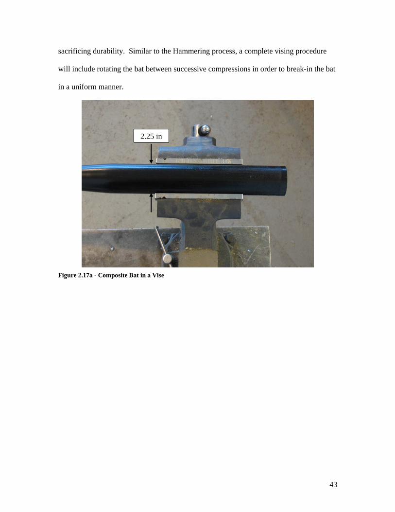
sacrificing durability. Similar to the Hammering process, a complete vising procedure

will include rotating the bat between successive compressions in order to break-in the bat

in a uniform manner.

2.25 in

Figure 2.17a - Composite Bat in a Vise

43

1.75 in

Figure 2.17b - Composite Bat Compressed in a Vise

Bats that have undergone ABI processes experience decreased durability and

improved performance that are both proportional to the severity of the ABI process. The

more severe the process, the more performance will increase and the lower durability will

be.

Proponents of ABI processes claim they should not be considered doctoring methods

because they are equivalent to hitting thousands of balls with a particular bat. In this

study, bats that have undergone ABI treatments are considered to be doctored because the

bats’ physical properties have been unnaturally altered in an attempt to improve the bats’

performance. The claim that ABI processes are equivalent to NBI processes has been

investigated in this study. Due to the fact that hammering bats induces bat stresses less

than those generated when a player actually hits a ball, the effects of hammering have not

been studied in this research.

44

2.5.5 Bat Painting

Bat painting describes the process of painting a bat whose performance exceeds

certification standards to look like a certified bat. This is done so that high performing,

uncertified bats, such as titanium bats, can be used in leagues which would normally not

allow them.

The procedure for painting a bat includes removing its stock graphics, and replacing

them with replications of graphics that can be found on certified bats. The major

difficulties in painting bats are dampening the characteristic “ping” noise made by

titanium bats, finding a paint that can stand up to the extreme flexing the barrel walls

experience, and using the best graphic reproductions. If these issues are not properly

addressed, painted bats can be easily identified. As a result, most players do not paint

their own bats; they have them done by one of three well known bat painters in the

United States.

2.6 Bat Models

The ability to compare direct and indirect performance measurements to computer

simulations is useful to verify that measured results follow logical trends. In addition,

computer modeling is both practical and useful for analyzing difficult to measure events,

such as the bat-ball collision. Herein, computer modeling will be used to verify modal

analysis measurements of various bat constructions and to study the effects of bat altering

on indirect performance characteristics.

To date, a relatively small number of articles describing FE modeling of bats have

been published. Smith [2.31] modeled the bat and ball collision of a wood and a single

wall aluminum bat, paying close attention to the stress levels generated in the bat as a

45

result of the collision and the post-impact rebound speed of the ball. In his work, Smith

used 8-node solid elements to represent the wood bat and 4-node shell elements to

represent the aluminum bat. The stress levels and ball rebound speeds predicted in

numerical simulations were consistent with experimentally measured values.

In a more recent publication, Nicholls [2.32] modeled the bat ball collision and

focused her analysis on post-impact ball velocity. In her work, Nicholls also modeled a

wood and a single wall aluminum bat; both of the bats were modeled using 8-node solid

elements. Results of Nicholls’ numerical simulation also agreed well with experimental

data.

Another finite element model investigating the bat ball collision has been developed

by Mustone [2.33]. As in the previously described studies, Mustone also modeled a

wood and a single wall aluminum bat. Mustone used 8-node solid elements in his wood

bat model, and 4-node shell elements in the aluminum bat model. Prior to his

investigation of the bat ball collision, Mustone calibrated his bat models by conducting an

eigenvalue analysis on them and comparing the results to measured values obtained using

modal analysis techniques. In this analysis, only the frequencies of the first two flexural

bending mode shapes are reported for both bat models, and all numerical results are

within 8% of experimentally measured frequency values. In addition to achieving a

strong correlation between simulated and measured dynamic bat properties, bat

performance data from Mustone’s impact model also correlated well with measured

performance values.

Irvine [2.34] has conducted research in which the vibrational response of a wood and

a single wall aluminum bat have been modeled with finite element software. In his

46

model, the wood bat was modeled using 8-node solid elements and the aluminum bat was

modeled using a combination of shell and solid elements. In addition to reporting the

natural flexural frequencies of both bats, Irvine also reported the hoop mode frequencies

of the aluminum bat. Though the values obtained in his numerical simulation seem

reasonable, their accuracy of cannot be commented on because no comparison with

measured vibration data was provided.

2.7 Summary

The focus of this chapter has been to review the current research relevant to baseball

and softball bats. In doing so, bat testing methods and performance metrics have been

examined and compared. Indirect performance characteristics have also been defined and

reviewed with an emphasis on their relation to performance trends. Computer modeling

of bats has been investigated and was found to correlate well with measured

characteristics. Finally, the most common bat doctoring methods have been defined and

discussed.

In the following chapters the previous topics will be expanded upon utilizing

techniques such as performance testing, barrel compression, modal analysis, and

computer modeling. Extensive studies regarding bat doctoring efficiency and the bat-ball

collision have been carried out and will be reviewed, and a computer model will be used

to verify the results.

47

REFERENCES

2.1 Smith, L. V., Why ASTM F2219? SGMA Annual Meeting, Dallas, TX. October

2, 2003. 2.2 Naruo, T., and F. Sato. Performance of baseball bats. Proceedings of 5th Japan

International Society of Advanced Material Processes. Engineering Symposium, (1997): 1311-1316.

2.3 Brooks, R., S. Knowles, and J.S.B. Mather. Design and construction of a high

performance composite cricket bat. Proceedings of ICCM-11. Gold Coast, Australia. July 1997.

2.4 Nishiwaki, T. Designing of CFRP baseball bats. SAMPE Journal. 38.2

(March/April 2002) : 80-82. 2.5 Russell, D. Indirect performance measures. Proceedings from Bat Ball 102.

Pullman, WA. June 29-30, 2004. 2.6 Nathan, A., D. Russell, and L. Smith. The physics of the trampoline effect in baseball and softball bats. Proceedings of ISEA 2005. Davis, CA. September 2004. 2.7 Noble, L., and J. Eck. Effects of selected softball bat loading strategies in impulse reaction impulse. Medicine and Science in Sports and Exercise. 18.1 (1986) : 50-58. 2.8 House, G. Chapter 10: Baseball and softball bats. Sports and Fitness Equipment Design. Ed. E. Kreighbaum. Human Kinetics Publishers, 1995. ISBN: 087322695X. 2.9 Adair, R. The Physics of Baseball. Third Edition. Perennial: New York. 2002. ISBN: 0060084367. 2.10 Bahill, T., and W. Karnavas. The ideal baseball bat. New Scientist. April, 6 1991 : 26-31. 2.11 Bahill, T. The ideal moment of inertia for a baseball or softball bat. IEEE Transactions on Systems, Man, and Cybernetics-Part A: Systems and Humans. 34.2 (March 2004) : 197-204. 2.12 Nicholls, R., et al. Bat kinematics in baseball: implications for ball exit velocity and player safety. Journal of Applied Biomechanics. Vol. 19 (2003) : 283-294.

48

2.13 Fleisig, G., et al. Relationship between bat mass properties and bat velocity. Sports Engineering. Vol. 5 (2002) : 1-8. 2.14 Smith, L. V., J. Broker, A. Nathan. A Study of Softball Player Swing Speed. Sports Dynamics Discovery and Application. Melbourne, Australia (2003): 12- 17. 2.15 Smith, L. V. Oklahoma Fastpitch Softball Field Study. NCAA Softball Rules Committee. November 18, 2004. 2.16 ASTM F2219-02e1. Standard test methods for measuring high speed bat performance factor. West Conshohocken, Pa. 2003. 2.17 ASTM F 1890-02. Standard test method for measuring softball bat performance factor. West Conshohocken, Pa. 2003. 2.18 F 1887-02. Standard test method for measuring the coefficient of restitution of baseballs and softballs. West Conshohocken, Pa. 2003. 2.19 Nathan, A. Characterizing the performance of baseball bats. American Journal of Physics. Vol. 71 (2002) : 134-143. 2.20 NCAA News Release. NCAA provisional standard for testing baseball bat performance. September 27, 1999. 2.21 Smith, L. Evaluating baseball bat performance. Sports Engineering. Vol. 4 (2001) : 205-214. 2.22 Procedure for measuring the flexibility of a golf clubhead. Revision 1.0 December 1, 2003. http://www.usga.org 2.23 Avitabile, P. Experimental modal analysis – a simple non-mathematical presentation. Sound and Vibration, February 2001. 2.24 Thomson, W. Theory of Vibration with Applications. Second Edition. Prentice- Hall: New Jersey. 1981. ISBN: 0139145230. 2.25 PCB Model 086C02 Spec Sheet. March, 8 2005. http://www.pcb.com 2.26 Smith, D. Vibration Measurement and Analysis. Butterworth and Co.: New York. 1989. ISBN: 0408041013. 2.27 Harris, C., ed. Shock and Vibration Handbook. Fourth Edition. McGraw Hill: New York. 1996. ISBN: 0070269203. 2.28 Russell, D. Kettering University. Private communication. March, 2005.

49

2.29 Craig, R. Mechanics of Materials. Second Edition. John Wiley and Sons: New York. 2001. 2.30 Russell, D. Indirect Performance Measures. Presentation at Bat-Ball 102 symposium. Pullman, WA. 2004. 2.31 Smith, L. V., Shenoy, M., Axtell, J.T. Simulated composite baseball bat impacts using numerical and experimental techniques. Abstract Proceedings of the Society for Experimental Mechanics. Spring Conference 2000. Orlando, FL. 2.32 Nichols, R. Mathematical modeling of bat-ball impact in baseball. Diss. University of Western Australia. 2003. 2.33 Mustone, T., J. Sherwood. Using LS-DYNA to develop a baseball bat performance and design tool. Proceedings of 6th international LS-DYNA Users Conference. Detroit, MI. April 2000. 2.34 Irvine, T. Baseball bat sound and vibration. Vibration data newsletter. December 2001. www.vibrationdata.com/Newsletters/December2001_NL.pdf

50

CHAPTER THREE

- BAT MODIFICATIONS -

3.1 Bat Doctoring Study

With the advent of a bat testing procedure that accurately ranks bats closely to their

on-field performance and the implementation of a reduced performance limit, many

softball players have turned to using altered bats in order to gain an advantage over their

opponents. The bat alteration methods most commonly used include wall shaving,

weighting, and various ABI techniques.

In this study, which will be referred to as the Doctoring Study, direct and indirect

performance measurements were conducted on altered bats in order to determine the

effect of the alterations. In addition, NBI bats were tested in order to determine how the

performance of an unaltered bat evolves with normal to extensive use. Finally, painted

bats were investigated by comparing them to the bats they are trying to imitate.

The procedure for the Doctoring Study included purchasing 26 ASA certified softball

bats and three popular bats that exceed the ASA performance standard. These 29 bats did

not all have the same construction; 19 were multi-wall composite, eight were multi-wall

aluminum, one was single wall aerospace grade aluminum, and one was a traditional

wood bat. Herein, these bats will be referred to by a bat code of the form XY##; where X

describes the construction style of the bat (S for single wall, M for multiple-wall), Y

describes the material the bat is made of (A for aluminum, C for composite). The lone

wood bat will be referred to as “wood.” One bat was chosen to be used as a standard bat

to verify the consistency of the indirect performance measurements, it was a multiple-

wall composite bat referred to as “std bat.” The std bat was tested intermittently for

51

barrel compression and vibration characteristics. Both modal analysis and barrel

compression were found to be very repeatable with standard deviations of less than 1.5%.

Data from the control bat can be found in Appendix 2. Table 3.1 is a list of all of the bats

included in this study.

Table 3.1 – List of all bats included in the bat doctoring study.

Bat Code Alteration method Bat Code Alteration methodMA01 Shaved MC08 ShavedMA02 Shaved MC09 ShavedMA03 Shaved MC10 RolledMA04 Shaved MC11 BCTMA05 Weighted MC12 ACTMA06 Shaved MC13 VicedMA07 Shaved MC14 Converted to FreakMA08 NBI MC15 Converted to Freak 98MC01 Weighted MC16 Converted to Velocite 2MC02 Shaved MC17 NBIMC03 Shaved MC18 NBIMC04 Rolled Std Bat NoneMC05 BCT SA01 WeightedMC06 ACT Wood WeightedMC07 Viced

Upon receipt of the bats, indirect performance measurements of each were made

using modal analysis (to determine flexural and hoop frequencies) and barrel

compression (to determine barrel stiffness). Next the performance of the bats was tested

following a procedure similar to that which is outlined in ASTM F 2219. The

performance testing procedure for the doctored bats differed in that three balls, instead of

six, were used per bat. The balls used on each bat were organized such that each time the

bats were tested the identical balls were used. In addition to controlling the balls used on

each bat, the bats were oriented in a consistent manner in the test fixture to ensure that the

identical bat locations were impacted during testing. After performance testing, indirect

52

performance tests were again performed and the bats were then divided into four groups;

the structural group, weighted group, the NBI group, and the painted group.

The structural group included 18 bats (12 multi-wall composite and six multi-wall

aluminum) and encompassed all of the bats that underwent wall shaving and ABI

processes. Each of the bats was sent to one of 11 well known bat doctors to be modified.

The bat doctors were chosen after numerous (no fewer than 16) well known doctors had

been identified through clandestine research conducted on various internet softball

websites and forums. The bat doctors were solicited for work without revealing that the

modified bats were for research purposes to assure that the modified bats were

representative of bats that could be obtained for use by an average player.

Four of the 12 composite bats were to be barrel shaved, while pairs of the remaining

composite bats underwent the ABI processes Rolling, BCT, ACT, and Vising. After the

bats had been modified, their indirect and direct performances were measured. Finally,

after the bats were performance tested, their indirect performances were measured again.

A flowchart depicting the process for the doctored bat group testing procedure can be

found in Appendix 3.

The weighted bat group consisted of four bats; a wood bat, single wall aluminum bat,

multiple-wall aluminum bat, and a multiple-wall composite bat. After initial testing,

these bats were weighted such that their stock moment of inertia was increased 20%.

This was accomplished by attaching lead tape and/or lead tire weights to the distal end of

the bats.

The amount of weight necessary to increase the bats’ moments of inertia 20% was

calculated using a form of the parallel axis theorem,

53

( )2d

MOIMOI

W i

d

a

⎟⎟⎠

⎞⎜⎜⎝

⎛

= , (3.1)

where Wa is the weight addition necessary to achieve the desired MOI, MOId is the

desired MOI, MOIi is the initial MOI, and d is the distance from the pivot point of the bat

to the location of weight addition. The MOI of a bat with the weight attached was

measured directly utilizing the MOI stand described in chapter two to verify the

prediction and the ability to add the appropriate amount of weight to the bats. After the

weight had been added, the BBS of each bat was determined; these measurements were

followed by another set of indirect performance measurements which were conducted

with the additional weight still attached to the bats.

The NBI group included three bats, two multiple-wall composite bats and one

multiple-wall aluminum bat. After they were initially tested, the NBI bats were each hit

500 times with ASA certified .44 COR, 375 lb compression balls in an indoor batting

cage. The bats were swung by mostly experienced softball and baseball players, and all

of the pitches were of the slow-pitch variety.* Figure 3.1 shows the batting cage used for

the NBI group of bats. After each bat had accumulated 500 impacts, the bats were tested

using indirect performance tests and then direct performance tests. These tests were

followed by 500 more hits on each bat and another round of indirect and direct

performance measurements. This cycle was continued until each bat had been hit 2000

times. A flowchart depicting the NBI group test procedure can be found in Appendix 4.

The painted bats group included the three multiple-wall composite bats which

exceeded the 2004 ASA performance limit. These bats were not ever tested for BBS as * A slow-pitch style pitch describes a ball thrown underhand that follows an arc between 6 and 12 feet before crossing the plate in the batter’s strike zone [3.1].

54

they are considerably more fragile than the other bats included in the study and often do

not survive the direct performance test. As a result, the only tests conducted on the

painted bats were visual inspections and indirect performance tests. The purpose of the

visual inspections were to determine how accurate the painted bats were compared to

actual bats. The purpose of conducting indirect performance measurements was to verify

that the bats returned to us by the bat doctors were in fact the bats we had sent to them.

The following sections will discuss how the characteristics of each of these bats

changed as a result of their modifications. Although indirect performance characteristics

were measured at four different times during the life of most of the bats in the Bat

Doctoring Study, most of the results are plotted showing only two of these data points as

the bat characteristics before the first BBS scan and after the second BBS scan are

superfluous in demonstrating the effect that the bat alterations have had. A table

containing all of the data from the Bat Doctoring Study is provided in Appendix 5.

55

Figure 3.1 – Batting cage used for NBI bat group

3.2 Results

3.2.1 Structural group - shaved bats

All of the composite and aluminum bats that were shaved in this study showed

measurable changes in barrel stiffness (as measured by barrel compression tests), hoop

frequencies and performance (as measured by BBS). None of the shaved bats showed an

appreciable change in flexural vibration, including the bats that had undergone handle

shaving in addition to barrel shaving. Most of the bats’ moments of inertia did not

change significantly due to the work done by the bat doctors, although two did, MC03

and MC09, because one of the bat doctors endloaded the bats in addition to shaving them.

56

The average change in MOI of the shaved bats, excluding the two bats that had been

endloaded (MC03 and MC09) was an increase of 2.3%. The slight increase in MOI is

likely the result of bat doctors attempting to maintain a bat’s original weight by adding

weight to the end caps to make up for the weight loss resulting from the shaving process.

Figure 3.2 shows the MOI changes in all of the shaved bats.

7000

7500

8000

8500

9000

9500

10000

10500

11000

MA01 MA02 MA03 MA04 MC02 MC03 MC08 MC09 MA06 MA07

Bat

MO

I (oz

in^2

)

Pre Doctored MOIPost Doctored MOI

Figure 3.2 - MOI Changes due to Shaving

As mentioned before, the flexural vibration characteristics of the shaved bats did not

change an appreciable amount, with even the largest change being less than 1.5%. Figure

3.3 shows the first resonant flexural frequency of the shaved bats before and after

doctoring.

57

0

50

100

150

200

250

MA01 MA02 MA03 MA04 MC02 MC03 MC08 MC09 MA06 MA07

Bat

Freq

uenc

y (H

z)Pre DoctoredPost Doctored

Figure 3.3 – Flexural Frequency Changes due to Shaving

The bats that were shaved showed an average decrease of 5% in their measured first

natural hoop frequency between the time when they were sent to the doctor and when

they were received from the doctor. The standard deviation of hoop frequency changes

was 2%. Figure 3.4 shows how each shaved bat’s hoop frequency changed as a result of

the shaving process.

The shaved bats showed an average stiffness decrease (as measured by barrel

compression) of 8% from the time when the bats were sent to doctors until they were

returned. The standard deviation for barrel stiffness changes was 8%, which is

comparatively higher than it was for hoop frequency. This suggests that tests for barrel

stiffness using barrel compression methods may be more sensitive than stiffness tests

using modal analysis. Figure 3.5 shows how the barrel stiffness of each shaved bat

changed as a result of the doctoring process.

58

In discussing the performance changes due to wall shaving, it was useful to look at

the composite and aluminum bats separately. The composite bats improved in BBS

performance on average 6.4 mph (or 7%) with a standard deviation of 1.0 mph (or 1%),

while the aluminum bats performance increased an average of 2.5 mph (or 3%) with a

standard deviation of 1.0 mph (or 1%). Figure 3.6 shows the performance increase of

each of the shaved bats.

1000

1100

1200

1300

1400

1500

1600

1700

MA01 MA02 MA03 MA04 MC02 MC03 MC08 MC09 MA06 MA07

Bat

Freq

uenc

y (H

z)

Pre DoctoredPost Doctored

Figure 3.4 – First Resonant Hoop Frequency Changes due to Shaving

59

4000

4500

5000

5500

6000

6500

7000

7500

8000

MA01 MA02 MA03 MA04 MC02 MC03 MC08 MC09 MA06 MA07

Bat

Stif

fnes

s (lb

/in)

Pre DoctoredPost Doctored

Figure 3.5 - Barrel Stiffness Changes due to Shaving

90

92

94

96

98

100

102

104

106

108

MA01 MA02 MA03 MA04 MC02 MC03 MC08 MC09 MA06 MA07

Bat

BB

S (m

ph)

Pre DoctoredPost Doctored

Figure 3.6 - Performance Changes due to Shaving

60

3.2.2 Structural group - ABI bats

Like the shaved bats, the eight bats that were sent out for ABI treatments did not

experience significant changes in either MOI or flexural stiffnesses, in fact none of the

first resonant flexural frequencies experienced measurable changes. Figures 3.7 and 3.8

show these trends. Bat MC13 showed an unexpected drop in MOI of 4.0%, and because

its mass and balance points remained consistent, the error is attributed to experimental

variation.

The first natural hoop frequencies of the ABI bats tended to decrease as a result of

the ABI processes. The hoop frequency decreases ranged from essentially no change

(0.5%) to 21.6%, and one bat’s hoop frequency increased 11.9%. The changes in the

hoop frequency of these bats due to ABI treatments are shown graphically in figure 3.9.

7000

7500

8000

8500

9000

9500

MC04 MC05 MC06 MC07 MC10 MC11 MC12 MC13

Bat

MO

I (oz

in^2

)

Pre DoctoredPost Doctored

Figure 3.7 - MOI changes due to ABI processes

61

100

120

140

160

180

200

220

MC04 MC05 MC06 MC07 MC10 MC11 MC12 MC13

Bat

Freq

uenc

y (H

z)Pre DoctoredPost Doctored

Figure 3.8 – Flexural Frequency Changes due to ABI Processes

1000

1100

1200

1300

1400

1500

1600

MC04 MC05 MC06 MC07 MC10 MC11 MC12 MC13

Bat

Freq

uenc

y (H

z)

Pre DoctoredPost Doctored

Figure 3.9 - First Resonant Hoop Frequency Changes due to ABI Processes

62

As expected, most of the ABI bats’ barrel stiffnesses also decreased after the bats had

been modified. The stiffnesses decreased from 1% to 54%, with three bats decreasing

more than 18% and the other five bats decreasing less than 7%. The changes in barrel

stiffness due to the ABI processes can be seen in figure 3.10.

Although the performance of all of the ABI bats increased, the magnitude of these

gains varied a great deal. The performance increases ranged from 0.66 mph (or 0.66%)

to 8.28 mph (or 8.53%) and seemed to be related to the severity of the process the bats

underwent. For example, the bat whose performance increased the most had visible signs

of damage as a result of the “proprietary” ABI technique, BCT. The performance

increases in all ABI bats are shown in figure 3.11, and an example of a bat which shows

significant damage due an ABI process (the BCT process) is shown in figure 3.12.

0

1000

2000

3000

4000

5000

6000

7000

8000

MC04 MC05 MC06 MC07 MC10 MC11 MC12 MC13

Bat

Stif

fnes

s (lb

/in)

Pre DoctoredPost Doctored

Figure 3.10 – Barrel Stiffness Changes due to ABI Processes

63

92

94

96

98

100

102

104

106

108

MC04 MC05 MC06 MC07 MC10 MC11 MC12 MC13

Bat

BB

S (m

ph)

Pre DoctoredPost Doctored

Figure 3.11 - Performance Changes due to ABI processes

Figure 3.12 - Visible Damage Resulting from BCT Treatment

The results from the structural bats group clearly shows that there are a number of

bat alteration methods which can improve bat performance. It appears that shaving

composite bats yields a greater performance advantage than shaving aluminum bats. This

64

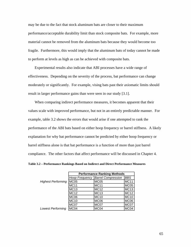
may be due to the fact that stock aluminum bats are closer to their maximum

performance/acceptable durability limit than stock composite bats. For example, more

material cannot be removed from the aluminum bats because they would become too

fragile. Furthermore, this would imply that the aluminum bats of today cannot be made

to perform at levels as high as can be achieved with composite bats.

Experimental results also indicate that ABI processes have a wide range of

effectiveness. Depending on the severity of the process, bat performance can change

moderately or significantly. For example, vising bats past their axiomatic limits should

result in larger performance gains than were seen in our study [3.1].

When comparing indirect performance measures, it becomes apparent that their

values scale with improved performance, but not in an entirely predictable manner. For

example, table 3.2 shows the errors that would arise if one attempted to rank the

performance of the ABI bats based on either hoop frequency or barrel stiffness. A likely

explanation for why bat performance cannot be predicted by either hoop frequency or

barrel stiffness alone is that bat performance is a function of more than just barrel

compliance. The other factors that affect performance will be discussed in Chapter 4.

Table 3.2 – Performance Rankings Based on Indirect and Direct Performance Measures

Hoop Frequency Barrel Compression BBSHighest Performing MC05 MC05 MC11

MC11 MC11 MC05MC13 MC12 MC13MC12 MC13 MC12MC06 MC10 MC10MC10 MC06 MC06MC07 MC07 MC07

Lowest Performing MC04 MC04 MC04

Performance Ranking Methods

65

3.2.3 Naturally Broken In Group

The NBI bats exhibited distinct trends in both direct and indirect performance

measures as a result of their break in procedure. The performance of all of the bats in the

study increased significantly after 500 impacts and essentially maintained that same

elevated performance level through the 2000 impacts in the study. It should be noted that

none of the bats in the study developed any visible signs of damage such as cracking or

denting due to the repeated impacts.

The indirect performance trends were found to be dependent on the material of which

the bat was made. Because there were only three bats tested in the study, it is impossible

to determine if the observed trends would apply to a much larger sampling of bats. One

trend observed in all bats was that flexural frequencies remained constant through the

study – this trend can be observed in figure 3.13.

0

50

100

150

200

250

MA08 MC17 MC18

Bat

Freq

uenc

y (H

z)

New 0 Hits500 Hits 1000 Hits1500 Hits

Figure 3.13 – Flexural frequency trends due to natural break in methods

66

The MOIs of the NBI bats were only measured prior to initial performance testing

because no weight was added to or removed from the bats. As a result, the same MOI

values were used in the BBS calculations for each round of performance tests. This

allowed for the truest assessment of performance change as it prevented the experimental

variation in measured MOI from introducing error into the BBS calculations.

Figure 3.14 shows how the performance of the NBI bats evolved during the study.

After the first 500 impacts each bat improved an average of 2.90 mph (or 3.02%).

Additional impacts were not observed to have a significant effect on further performance

changes.

The composite bats’ barrel stiffnesses were found to decrease with increased hits,

seemingly converging to some nominal, bat-dependent value. The multiple-wall bat’s

barrel stiffness followed a low order exponential increase, which also seemed to approach

a bat-dependent nominal value. These trends are shown in figure 3.15.

The hoop frequencies of the composite bats decreased with increased hits, seemingly

converging to a bat-dependent value. The multiple-wall aluminum bat’s hoop frequency

also decreased with increasing impacts, although the decrease followed a much shallower

slope than the composite bats. The aluminum bat’s hoop frequency also seemed to

converge to a specific value. The trends in hoop frequency are shown in figure 3.16.

Due to the fact that the NBI bats’ MOI’s remained constant through the study, it is

assumed that any observed performance increase was a result of a dramatic decrease in

barrel stiffness – which would enhance performance by improving the trampoline effect.

In this case, the indirect performance measures, which often scale with the trampoline

effect, would not be an accurate performance predictor for the bat, as the barrel

67

compression and hoop frequency behaved in inconsistent manners. The two indirect

performance measures of the composite bats followed the expected trends.

93

94

95

96

97

98

99

100

101

102

MA08 MC17 MC18

Bat

BB

S (m

ph)

0 Hits 500 Hits1000 Hits 1500 Hits2000 Hits

Figure 3.14 – BBS trends due to natural break in methods

4000

4500

5000

5500

6000

6500

7000

7500

8000

MA08 MC17 MC18

Bat

Stif

fnes

s (lb

/in)

New 0 Hits500 Hits 1000 Hits1500 Hits 2000 Hits

Figure 3.15 – Barrel stiffness trends due to natural break in methods

68

1050

1100

1150

1200

1250

1300

1350

1400

1450

1500

MA08 MC17 MC18

Bat

Freq

uenc

y (H

z)New 0 Hits500 Hits 1000 Hits1500 Hits

Figure 3.16 – Hoop frequency trends due to natural break in methods

3.2.4 Weighting group

The bats chosen for the weighting group represent the four most common bats

currently in use; multiple-wall composite, multiple-wall aluminum, single-wall

aluminum, and solid wood. These bats’ direct and indirect performance levels were

tested before and after their stock MOI’s were increased by 20%.* The MOI was

increased by adding weight to the distal end of each bat, in an attempt to simulate loading

strategies used by the popular bat doctors. Figure 3.17 shows how weight was added to

the bats. The actual amount of weight added to each bat can be found in Appendix 6.

* A 20% increase in MOI was chosen because in a previous study a bat whose MOI had increased nearly 20% experienced significant performance gains.

69

Lead Tape

Figure 3.17 - Method of Increasing MOI of Weight Group

As expected, neither the barrel stiffness or hoop frequency changed in any of the bats

as a result of the increased MOI. Vibrational data for the flexural frequencies of the bats

proved inconclusive; the effect of various loading strategies on flexural frequencies will

be examined in more detail in Chapters 4 and 5.

The performance of all the bats increased an average of 2.72 mph (or 2.95%) and can

be seen in figure 3.18. Possible causes for the performance increases and changes in

dynamic properties will be discussed in Chapter 4, when the effects of added weight on

performance and bat characteristics will be investigated in more detail.

70

84

86

88

90

92

94

96

98

100

SA01 Wood MC01 MA05

Bat

BB

S (m

ph)

StockWeighted

Figure 3.18 - Performance Changes due to End Loading

3.2.5 Painted group

While the visual inspection of the painted bats is a subjective process, figures 3.19-

3.27 demonstrate that bat doctors can convert bats with enough skill to fool, at the very

least, most casual observers. The pictures compare the stock bats, painted bats, and the

imitated bats. In addition, the end caps and knobs of each bat are compared. In the case

of most of the bats, the decals used for the most prominent graphics on the bat look

nearly identical to the graphics used on the real bats. Often, converted bats can stand out

because these graphics have been poorly applied and their edges appear to be raised off

of the surface of the bat, or because the text fonts and resolutions are not a perfect match.

Occasionally, the diameter of painted bats will exceed their allowable limit of 2.25

71

inches, thus allowing them to be identified by the ASA Ring Test.* Because the main

focus of investigating painted bats was to determine how accurate the imitations could be,

these bats were not performance tested.

Barrel compression testing was performed on two of the bats. Figure 3.28 shows the

barrel stiffness values of two of the painted bats before and after painting, neither bat’s

stiffness values changed more than 3%. Such a result is evidence that the bats that were

sent out to be painted were in fact returned to us. If that had not been the case the barrel

stiffnesses probably would have been inconsistent.

5500

5700

5900

6100

6300

6500

6700

6900

7100

7300

7500

MC14 MC15

Bat

Stif

fnes

s (lb

/in)

StockPainted

Figure 3.28 – Barrel Stiffness Comparison Before and After Painting

* The ASA Ring Test is a test that is in place to identify bats that have dented past allowable limits. The test involves sliding a ring with diameter 2.375 inches over the barrel of the bat. If the ring does not freely slide over the bat, the bat is not acceptable for use in play.

72

Stock Miken Velocit-e II Stock Miken Ultra Converted to Miken

Velocit-e II

Figure 3.20 - Ultra Converted to Velocit-e II

Figure 3.21 - Ultra Converted to Velocit-e II (knobs)

Figure 3.22 - Ultra converted to Velocit-e II (end caps)

73

Stock Miken Ultra II

Converted to Miken Freak

Stock Miken Freak

Figure 3.23 - Ultra II Converted to Freak

Figure 3.24 - Ultra II Converted to Freak (knobs)

Figure 3.25 - Ultra Ii converted to Freak (end caps)

74

Stock Miken Ultra II

Converted to Miken Freak 98

Stock Miken Freak 98

Figure 3.26 - Ultra II Converted to Freak 98

Figure 3.27 - Ultra II Converted to Freak 98 (knobs)

Figure 3.28 - Ultra II converted to Freak 98 (end caps)

75

3.3 Discussion

Testing has verified that there are many effective methods of doctoring some of

today’s most popular bats. Shaving composite bats resulted in the highest average

performance increase followed by ABI methods, NBI methods, end-loading, and then

shaving aluminum bats. Figure 3.29 shows these rankings graphically. It is unclear how

these bat modifications interact, but it is reasonable to assume that the performance

increases due to some of the methods should be additive. For example, a shaved

composite bat that was endloaded should have a performance increase of nearly 10%.

0%

1%

2%

3%

4%

5%

6%

7%

Shaved Composite ABI NBI Weighted Bats Shaved Aluminum

Doctoring Methods

Per

form

ance

Incr

ease

(%)

Figure 3.29 - Effectiveness of Various Doctoring Methods

ABI methods resulted in the widest ranges of performance changes, with increases

from 0.66 mph (or 0.66%) to 8.28 mph (or 8.53%). The performance increases due to

these methods seem to be dependent on the severity of the process.

Testing showed that regular use of some of the most popular bats today can result in

performance increases comparable to some ABI treatments. This poses potential

76

problems for regulating agencies as it would be very difficult to tell the difference

between an altered bat and a naturally broken in bat. Furthermore, comparing the NBI

and ABI bats, it becomes clear that in terms of indirect performance characteristics and

BBS values, three ABI processes (rolling, ACT, and vising) are equivalent to naturally

breaking a bat in.

Testing has shown that a BBS scan usually does not improve performance levels in

the same way natural break-in does. In addition, natural break-in causes greater changes

in bats’ indirect performance measures. These results imply that if regulating agencies

want to test bats that have already reached their maximum naturally attainable

performance level, it would not be sufficient to simply increase the number of impacts

used in a certified BBS scan by a small amount.

It has also been shown that indirect performance measurements follow general trends

with bat increasing performance. These trends, however, contain a considerable amount

of scatter. Figures 3.30 and 3.31 show how hoop frequencies and barrel stiffnesses of the

doctored bats scaled with performance.

77

94

96

98

100

102

104

106

108

1000 1100 1200 1300 1400 1500 1600 1700 1800

Hoop Frequency (Hz)

BB

S (m

ph)

Figure 3.30 – Hoop frequencies plotted against bat performance

94

96

98

100

102

104

106

108

2000 3000 4000 5000 6000 7000 8000 9000 10000

Barrel Stiffness (lb/in)

BB

S (m

ph)

Figure 3.31 – Barrel stiffnesses plotted against bat performance

78

The following chapter will investigate the topic of added weight/increased MOI in

greater detail. In doing so, a clearer understanding of the bat-ball collision will be

realized.

79

REFERENCES 3.1 Jones, John. Pioneer of the vising method. Private communication. September

8, 2005 3.2 Official rules of softball – umpire edition. 2004 edition. Oklahoma City, OK:

Amateur Softball Association of America, 2004.

80

CHAPTER FOUR

- BAT WEIGHT DISTRIBUTIONS -

4.1 – Weighting Study

Results from the weighted bats group in the Doctored Bat Study showed that adding

weight to the distal end of bats of all construction types improved performance.

Consideration of the compliance of the impacting bodies suggests that the contribution of

weight distributions is non-trivial. Few publications have investigated this phenomenon,

although several studies pertaining to the contact time of the bat-ball collision have been

completed. Nathan [4.1] and Adair [4.2] both concluded that the bat-ball collision was so

short in duration (between 0.6 and 1.0 ms) that the ball rebound could not be affected by

the boundary conditions of the bat knob.

One may assume, therefore, that weight added sufficiently distant from the impact

location will not affect a bat’s hitting performance (except for the way in which an

increased MOI slows swing speed). In order to further investigate the effect of increased

MOI/weight on performance, the Weighting Study was devised.

The Weighting study involved adding weight to initially un-weighted bats at 12

different locations. The amount of weight that was added varied with each location, but

was governed by the requirement that the weight addition was to increase the bat’s

original MOI by 10%. A 10% increase was chosen because the 20% increase used in the

weighted bat group from the bat doctoring study would have required adding

unreasonable amounts of weight to the bat (over 3.5 pounds).

Each time the bat was re-weighted, the test protocol again followed ASTM 2219,

where the BBCOR was measured before and after each weight amount was applied.

81

Unweighted tests were conducted to quantify how the performance of the bats was

evolving due to the repeated impacts. Four bats were chosen for the Weighting study; a

solid wood bat, single wall aluminum bat, multiple-wall aluminum bat, and a multiple-

wall composite bat. The wood bat was tested at 110 mph, while the remaining bats were

tested at 90 mph in order to avoid denting or cracking during the 100+ impacts required

in the study.

Figure 4.1 is a schematic showing the approximate locations where the bat was

impacted, Q, and where weight was added to it, d. The additional weight, in the form of

adhesive-backed lead tire weights, was attached to the bat using reinforced adhesive.

Figures 4.2-4.6 show specific examples of how the weight was actually fixed to the bats.

Figure 4.1 - Schematic of bat impact and weight addition locations

82

Figure 4.2 - MOI Study weight addition example 1

Figure 4.3 - MOI Study weight addition example 2

83

Figure 4.4 - MOI Study weight addition example 3

Figure 4.5 - MOI Study weight addition example 4

84

Figure 4.6 - MOI Study weight addition example 5

The amount of weight necessary to increase each bat’s MOI 10% was found using the

parallel axis theorem. Appendix 7 compares the target and actual weight additions for

each weight location. The 10% MOI increase of all weight locations was verified by

measuring the MOI of bat at several weight locations. In all cases its MOI was observed

to be within 1% of the target values.

Modal analysis was performed on the bats with and without weight attached to

determine how the mode shapes and node locations were affected by the added weight.

4.2 – Results

In Chapter 3 BBS was used as the performance metric because it provided the most

accurate method for comparing how different bats would perform relative to one another

when swung by players. In this chapter, BBCOR will be used so that performance

changes can be compared, independent of the bats’ MOI.

Recall the formulation of BBCOR, given as

85

( ripii

rBB vv

IvmQ

vve ++=

2

) . (2.10)

Applied to the Weighting Study, the terms, , , and were constant. This implies

that any BBCOR increase, for a given impact location (Q=constant), must be a result of

an increased rebound speed, .

iv m pI

rv

4.2.1 – Wood bat

Figure 4.7 shows the BBCOR as a function of weight location for the three impact

locations. The plot also shows a baseline performance level which is the BBCOR value

with no weight attached to the bat. This baseline measurement was taken to verify that

bat performance did not change as a result of the repeated impacts. The shaded column

on the plot identifies the region in which the bat was impacted. The plot reveals multiple

trends in the bat-ball collision. First, the impact location that produces the highest

BBCOR changes with the location of weight addition, and second, there seems to be a

finite distance from the impact location at which the addition of weight has no effect on

the bat-ball collision.

86

0.34

0.35

0.36

0.37

0.38

0.39

0.4

0.41

0 2 4 6 8 10 12 14 16 18 20 22 24 26 28

Location of Weight Addition (in)

BB

CO

R21 inch impacts21.5 inch impacts22 inch impacts

21 inch baseline

Figure 4.7 – BBCOR as a function of weight location – wood bat

The BBCOR of the wood bat reached a maximum value when weight was added 5-6

inches inside (toward the knob end of the bat) of the impact location. The distance (from

the weight to the impact location) at which the added weight had no effect on BBCOR

values was beyond about 9 inches.

4.2.2 – Single wall aluminum bat

The single wall aluminum bat, whose trends are shown in figure 4.8, yielded similar

results to the wood bat.

87

0.43

0.44

0.45

0.46

0.47

0.48

0.49

0.5

0.51

0 2 4 6 8 10 12 14 16 18 20 22 24 26 28

Location of Weight Addition (in)

BB

CO

R20 inch impacts20.5 inch impacts21 inch impacts

20.5 inch baseline

Figure 4.8 - BBCOR as a function of weight location – single wall aluminum bat

In this case the distance at which weight additions had no effect on BBCOR values was

beyond about 12 inches, and the distance at which BBCOR was optimized was between

5-6 inches inside the impact location.

4.2.3 – Multiple-wall aluminum bat

As shown in figure 4.9, the high speed testing data collected from the multiple-wall

aluminum bat exhibited more scatter than the wood, single wall aluminum, or the soon to

be discussed multiple-wall composite bats.

88

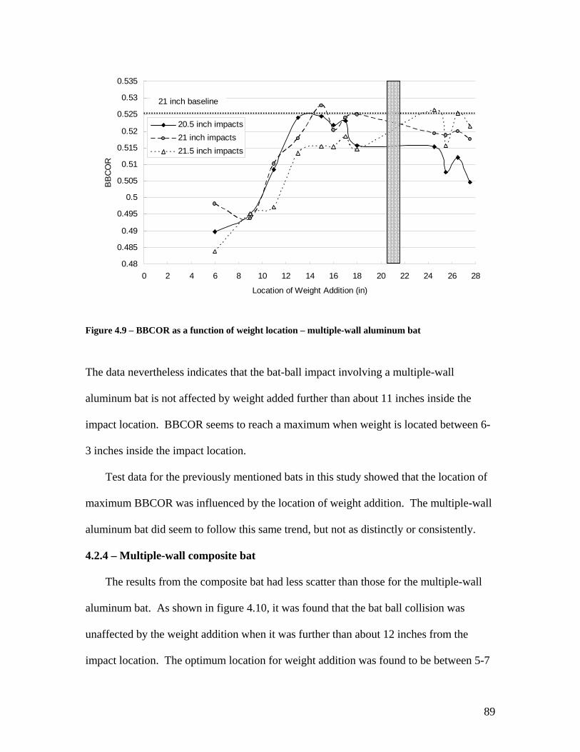
0.48

0.485

0.49

0.495

0.5

0.505

0.51

0.515

0.52

0.525

0.53

0.535

0 2 4 6 8 10 12 14 16 18 20 22 24 26 28

Location of Weight Addition (in)

BB

CO

R

20.5 inch impacts21 inch impacts21.5 inch impacts

21 inch baseline

Figure 4.9 – BBCOR as a function of weight location – multiple-wall aluminum bat

The data nevertheless indicates that the bat-ball impact involving a multiple-wall

aluminum bat is not affected by weight added further than about 11 inches inside the

impact location. BBCOR seems to reach a maximum when weight is located between 6-

3 inches inside the impact location.

Test data for the previously mentioned bats in this study showed that the location of

maximum BBCOR was influenced by the location of weight addition. The multiple-wall

aluminum bat did seem to follow this same trend, but not as distinctly or consistently.

4.2.4 – Multiple-wall composite bat

The results from the composite bat had less scatter than those for the multiple-wall

aluminum bat. As shown in figure 4.10, it was found that the bat ball collision was

unaffected by the weight addition when it was further than about 12 inches from the

impact location. The optimum location for weight addition was found to be between 5-7

89

inches from impact location. The composite bat also demonstrated the trend that the

impact location providing the maximum BBCOR was dependent on the location of the

weight addition.

0.51

0.52

0.53

0.54

0.55

0.56

0.57

0.58

0 2 4 6 8 10 12 14 16 18 20 22 24 26 28

Location of Weight Addition (in)

BB

CO

R

20.5 inch impacts21 inch impacts21.5 inch impacts

21 inch baseline

Figure 4.10 – BBCOR as a function of weight location – multiple-wall composite bat

4.3 – Discussion

Testing shows that the location at which weight is added to a bat does have a direct

effect on performance. The performance of each bat reached a maximum when the

weight was located at a specific distance from the impact location. This location was

unique for each bat, although it followed the same trend in all bats.

The fact that BBCOR changed as a function of the weight location on all of the bats,

including the wood bat, implies that the change in performance was a related to the bats’

flexural responses.

90

Modal analysis was used as a means of comparing the bats’ flexural responses. A

full modal analysis was performed on the single wall aluminum and multiple-wall

composite bats* with and without weight attached to the location which provided the

maximum BBCOR value. This analysis was done in order to determine if the flexural

properties of the bats, such as bending frequencies or node locations, changed as a result

of weight addition.

Figures 4.11-4.14 are waterfall plots showing the first two flexural mode shapes of

the aluminum and composite bats and their relative magnitudes. The node locations of

each mode (the location at which the plot crosses zero on the amplitude axis) can also be

seen in each of the plots. It should be noted that on the plots of the weighted bats, the

location on the bat where weight was added can be seen by a localized spike in the mode

shape.

* The wood bat could not be analyzed because it fractured after performance testing. The multiple wall aluminum bat data had large scatter and was difficult to interpret.

91

Amplitude (db)

Bat Length (in)

Frequency (Hz/3)

Figure 4.11 - Waterfall plot of single wall aluminum: no weight

Weight addition

Amplitude (db)

Bat Length (in)

Frequency (Hz/3)

Figure 4.12 - Waterfall plot of single wall aluminum: weight at 17” location

92

Noisy signal

Amplitude (db)

Bat Length (in)

Frequency (Hz/3)

Figure 4.13 - Waterfall plot of multiple-wall composite: no weight

Weight addition

Amplitude (db)

Bat Length (in)

Frequency (Hz/3)

Figure 4.2 - Waterfall plot of multiple-wall composite: weight at 17” location

93

The added weight seemed to have one consistent effect on flexural frequencies in that

each decreased less than 10%, except for the second flexural mode of the composite bat,

which increased less than 5%. None of the node locations for any of the bats changed

more than one inch. The nodes that did move generally shifted toward the knob end of

the bat. The remaining trend shown in the plots is that the addition of weight seemed to

attenuate the second flexural bending modes. It is unclear whether the apparent

attenuation was a result of the small node location shift or an actual decrease in vibration

amplitude. The results of modal testing have been insufficient in determining whether

the performance trends were a result of the bats’ vibrational characteristics.

The most significant performance trend observed in the Weighting Study was that

the impact location providing the maximum BBCOR was a function of the weight

location. In addition there does appear to be a region of the bat where added weight did

not affect the bat-ball collision.

Due to the fact that the wood bat showed performance increase it is reasonable to

conclude that the performance increases observed in this study are not (at least entirely) a

result of an improved trampoline effect. One explanation for why various loading

conditions improve performance can be derived from the fact that the ball COR measured

off of a rigid wall is higher than it is off of a recoiling wall [4.3]. This idea can be

converted to the bat-ball impact by closely examining the impact. As the ball impacts a

bat, the bat deflects a small amount during the time in which they are in contact. In

addition to this global deflection (bending) that occurs and is shown in figure 4.15, a

94

hollow bat also compresses circumferentially. For a given net impact speed and impact

location, each bat will bend and might compress a set amount.

Before further analysis, it is helpful to avoid thinking of a bat in a traditional, global

sense. Instead it can be useful to think of a bat as the sum of many small pieces all of

which can have an individual weight and inertia, figure 4.16 shows such a bat. It is

important to note that the sum of each of these pieces’ weights and inertias will remain

constant. Just as in the Weighting Study where the weight distribution was altered while

maintaining a constant MOI. If the weight, and therefore inertia, of a small piece of the

bat near the impact location is increased, the local inertia will hinder the bat’s global

tendency to bend. If the bat is hollow, the added inertia will also resist the barrel

compression due to the impact.

95

Before impact

Reference lines

During impact

Figure 4.15 – High speed video capture of bat-ball impact

Figure 4.16 – Discretized softball bat

96

The effect of the reduced bending in the bat makes more energy available to be

returned to the ball. This can account for the performance increase observed in wood

bats as well as the other bats involved in the study. The fact that the hollow bats’

performances decreased as weight was added closer to the impact location supports the

idea that the local increase in inertia resisting the bat’s tendency to compress reduces the

efficiency of the trampoline effect. This would imply that a solid bat’s performance

should continue to increase as weight is added closer and closer to the impact location,

but this has not been confirmed in this small scale study.

97

REFERENCES 4.1 Nathan, A. Bat performance metrics. Presentation at Bat-Ball 102 symposium.

Pullman, WA. 2004. 4.2 Adair, R. The Physics of Baseball. Third Edition. Perennial: New York. 2002.

ISBN:0060084367. 4.3 Experimental and numerical characterization of softballs. Duris, J. Unpublished

Master’s Thesis. December 2004.

98

CHAPTER FIVE

- COMPUTER MODELING -

5.1 – Modeling Methods

In this work, finite element modeling was used to verify the results of physical

characteristics (MOI, balance point, etc) and modal analysis testing. The finite element

software package used was LS-DYNA, double-precision version 970 (Livermore

Software Technology Corporation).

A complete discussion regarding the fundamentals of finite element methods is

beyond the scope of this research. The following discussion of finite element methods

will be limited to the methods used in this study. The reader is referred to [5.1], [5.2],

[5.3] for further information on general finite element theory.

A dynamic finite element analysis can be performed using two different calculation

methods, explicit and implicit time integration. The explicit method calculates the nodal

displacement matrix { using the general difference method }D

{ } { } { } { } { }( ),...,,, 11 −+ = nnnnn DDDDfD &&& , 5.1

combined with the equation of motion evaluated at time step n. The result is a {D}

matrix that is based solely on historical information [5.1].

The implicit method calculates the nodal displacement matrix using the general

difference method

{ } { } { } { } { } { }( ),...,,,, 111 nnnnnn DDDDDfD &&&&&&+++ = 5.2

which is combined with the equation of motion at time step 1+n . The equation of

motion at time step is written as 1+n

[ ]{ } [ ]{ } [ ]{ } { } 1111 ++++ =++ nnnn RDKDCDM &&& . 5.3

99

The major difference between the formulation of the explicit and implicit methods is

that the former is based entirely on historical data and the latter is only partially based on

historical data. As a result of their unique formulations, each of these methods exhibit

distinctive characteristics.

The explicit method is conditionally stable – which means that the numerical process

will be stable unless a model dependent critical time step is exceeded. A benefit of this

method is that the numerical process is greatly simplified for each time step because the

coefficient matrix of { (the equivalent stiffness matrix) can be diagonalized. As a

result, each time step requires relatively small computational power. The drawback to

the explicit method is that acceptable time step sizes are so small that the solution time

can be large due to the high number of equations that must be solved.

}D

The implicit method is unconditionally stable – which means that the numerical

process is stable regardless of the time step size. One benefit of this method is that fewer

time steps are necessary during an analysis, although if time steps become too large

accuracy can suffer. The drawback to the implicit method is that the coefficient matrix of

cannot be diagonalized, the result of this is a relatively large amount of computing

power is necessary to solve the equations at each time step.

{ }D

As a result of their distinct characteristics, these methods should not be used

interchangeably when a high degree of computing efficiency is desired. Generally, the

explicit method is used when the simulated event occurs on a short time scale so that the

benefit of faster computation time is not negated by the number of time steps necessary to

describe the event. Impacts and explosions are examples of events that the explicit

method is well suited for. The implicit method is most often used for simulations of

100

events occurring on much larger time scales, such as earthquakes or slow ramp loads.

Modal analysis problems are also candidates for the implicit solution method.

In a simplified modal analysis problem (neglecting damping effects), the equation for

free vibration

[ ] [ ]( ){ } { }02 =− DMK ω 5.4

must be solved [5.1]. Equation (5.4) is an eigenvalue problem, where [K] is the global

stiffness matrix, is an eigenvalue whose natural frequency is 2ω ω , [M] is the global

mass matrix, and{ }D is the displacement matrix which is associated with nodal

displacements and accelerations by

{ } { } tDD ωsin= 5.5

and

{ } { } tDD ωω sin2−=&& . 5.6

The LS-DYNA software suite offers many element options. In this work, 8-node

solid brick elements were used. The brick elements employed selective reduced

integration without rotational degrees of freedom (LS-DYNA solid element formulation

2). These elements were fully integrated over the deviatoric stress field and had one

integraton point in the pressure field. Solution time would have been reduced by using

shell elements. They were not used, however, since the preprocessor only supported

constant thickness shell elements. Thick shell elements were considered because they are

not a constant thickness element. The thick shell elements were not implemented

because they were not compatible with LS-DYNA’s implicit eigenvalue analysis.

101

In the following sections, the results of a convergence study are presented.

Frequency and mode shapes from experimental modal analysis are compared to

numerical predictions for a wood bat and a single and multiple-wall aluminum bat.

5.2 – Convergence study

When modeling a hollow baseball or softball bat, there are three methods for altering

the mesh density in the model. One method involves changing the number of elements

along the length of the bat (longitudinal elements); another involves changing the number

of elements around the circumference of the bat (circumferential elements); finally, the

number of elements through the thickness of the bat walls can be manipulated.

The effect that each of these parameters had on solution accuracy and solution time

were studied to find the most accurate and efficient method for modeling a bat. The

profile used during the convergence study was a simplified single wall aluminum bat

which did not include an end cap or knob. The results were normalized using the finest

mesh density

Figures 5.1 and 5.2 show how the normalized flexural and hoop frequencies

converge as the number of elements along the length of the bat increase. In these

simulations, the number of elements through the wall thickness and around the

circumference of the bat were held constant at 1 and 72 respectively.

102

-80%

-70%

-60%

-50%

-40%

-30%

-20%

-10%

0%

10%

0 20 40 60 80 100 120 140 160

Number of Longitudinal Elements

Per

cent

Diff

eren

ce

1st2nd3rd

Flexural Modes

Figure 5.1 – Flexural frequency convergence due to longitudinal element variations

-80%

-70%

-60%

-50%

-40%

-30%

-20%

-10%

0%

10%

0 20 40 60 80 100 120 140 160

Number of Longitudinal Elements

Per

cent

Diff

eren

ce 1st

2nd

Hoop Modes

Figure 5.2 – Hoop frequency convergence due to longitudinal element variations

103

The plots depicting the convergence due to increasing the number of longitudinal

elements imply that too few elements result in an overly stiff model. This would be

expected as larger elements provide a poor representation of bending.

Figures 5.3 and 5.4 show how the flexural and hoop frequencies are affected by

changing the number of elements around the circumference of the bat. In these

simulations the number of elements along the length of the bat and through the thickness

were held constant at 34 and 1 respectively.

-10%

0%

10%

20%

30%

40%

50%

60%

70%

80%

0 50 100 150 200 250 300 350 400

Number of Circumferential Elements

Per

cent

Diff

eren

ce

1st2nd3rd

Flexural Modes

Figure 5.3 - Flexural frequency convergence due to circumferential element variations

104

-80%

-70%

-60%

-50%

-40%

-30%

-20%

-10%

0%

10%

0 50 100 150 200 250 300 350 400

Number of Circumferential Elements

Per

cent

Diff

eren

ce

1st2nd

Hoop Modes

Figure 5.4 – Hoop frequency convergence due to circumferential element variations

The flexural frequency convergence due to increasing elements around the bat

circumference did not follow the same trends observed in other cases. In figure 5.3 the

percent difference does not seem to converge to any value. One possible reason for this

result is that a very high aspect ratio of 51:1 occurs in the finest mesh density.

Convergence of the hoop frequencies does follow the expected trend in that as the

number of elements increase, the model becomes better suited to describe bending

motion.

The effects of altering the number of elements through the wall thickness are shown

in figures 5.5 and 5.6. In these simulations the number of elements along the length of

the bat and around its circumference were held constant at 102 and 120 respectively.

105

-80%

-70%

-60%

-50%

-40%

-30%

-20%

-10%

0%

10%

0 1 2 3 4 5

Number of Elements Through the Thickness

Per

cent

Diff

eren

ce

1st2nd3rd

Flexural Modes

Figure 5.5 – Flexural frequency convergence due to through the thickness element variations

-10%

0%

10%

20%

30%

40%

50%

60%

70%

80%

0 1 2 3 4 5

Number of Elements Through the Thickness

Per

cent

Diff

eren

ce

1st

2nd

Hoop Modes

Figure 5.6 - Hoop frequency convergence due to through the thickness element variations

106

The convergence plots demonstrate that, in general, increasing mesh density reduces

the model’s stiffness. Figures 5.3 and 5.6 stand out because their stiffnesses increase as

more elements are added to the model. Investigation into the details of the brick elements

used in the convergence study revealed they were linear elements, which do not

incorporate incompatible modes. Such elements tend to show increased stiffness as

aspect ratios increase due to element locking, which helps explain the observed trends.

The convergence study showed that flexural response of the model is dominated by

the number of longitudinal elements, while hoop response is dominated by the number of

circumferential elements and elements through the thickness.

While the highest mesh densities provided the most accurate results when modeling

bats, the solution time for the higher mesh densities were large (on the order of 7 hours).

A compromise between solution convergence and solution time was made using a 95%

convergence threshold. Accordingly, the mesh density for all bat models was 102

elements along the length of the bat, 180 elements around its circumference, and 2

elements through the thickness. The largest aspect ratio using this configuration was

relatively large at 30:1, but still provided results that were consistent with measured

values.

5.3.1 – Bat models

Three bats have been modeled in this study, a wood bat, a single wall aluminum bat,

and a multiple-wall aluminum bat. The profiles of the hollow bats were found by

dissecting a sample bat and measuring wall thicknesses with calipers. It was assumed

that neither the knob nor end cap of the bats were critical to the response of the hollow

bats. They were included in the model using simplified geometries. The properties for

107

each material used in the bat models were defined according to actual material properties

(Appendices F and G include the bat profiles and material definitions used to model the

bats) [5.4]. The densities of the end cap and knob were manipulated so that the mass,

mass center, and MOI of the models matched the measured values of the modeled bats.

Figures 5.7-5.14 are examples of all of the modeled bats.

Figure 5.7 – Wood bat model

108

Figure 5.8 – Sectioned view of wood bat model

Figure 5.9 – Single wall aluminum bat model

109

Figure 5.10 – Sectioned view of single wall aluminum bat model

Figure 5.11 – Views of knob used on aluminum bat models

110

Figure 5.12 – Multiple-wall aluminum bat model

Figure 5.13 – Sectioned view of multiple-wall aluminum bat model

111

Figure 5.14 – Close-up of sectioned view of multiple-wall aluminum bat model

5.3.2 – Solid wood bat

As shown in figure 5.8, the wood bat was meshed in two separate pieces and then

combined into one. This was done to prevent the use of inconsistently shaped elements.

Since the wood bat response was not of primary interest for this study, it was modeled

without a knob and as an isotropic material. This shifted the balance point of the bat

toward the knob end of the bat and reduced the overall weight of the bat less than 2%.

Modeling the solid wood bat resulted in flexural frequencies that were very similar to

measured values. In addition to the model’s accurate representation of vibrational

characteristics, the bat’s physical properties including its center of mass and moment of

inertia were well represented by the model. Tables 5.1 and 5.2 compare the numerical

and measured vibrational and physical characteristics of the wood bat. The first two

112

flexural frequencies deviated less than 4% from measured values. The center of mass of

the numerical model was nearly 1% further from the knob than the actual bat, and the

MOI was less than 1% from its measured value.

Table 5.1 - Measured and simulated vibrational characteristics of a solid wood bat

Numerical Results Measured values % error1st flexural mode (Hz) 149 153 2.6%2nd flexural mode (Hz) 552 536 -3.0% Table 5.2 - Measured and simulated physical characteristics of a solid wood bat

Numerical Results Measured Values % errorMass (oz) 33.86 34.25 -1.1%Center of Mass (in) 22.32 22.11 0.9%MOI (oz in^2) 11437 11534 -0.8%

The wood bat model was also used to examine how adding weight to the distal end

of the bat (as discussed in Chapter 3) affected its vibrational characteristics. In the

model, weight was added to the distal end of the wood bat by adding a set of shell

elements around the circumference of the last half inch of the bat. These elements were

merged to the existing solid elements. The modulus of these elements were 0.1% of the

wood so they would not affect the bat’s flexural response. The comparison with

experimental measurements was generally favorable, as shown in tables 5.3 and 5.4.

Table 5.3 - Measured and simulated vibrational characteristics of a weighted solid wood bat

Numerical Results Measured values % error1st flexural mode (Hz) 151 158 4.4%2nd flexural mode (Hz) 561 542 -3.5% Table 5.4 - Measured and simulated physical characteristics of a weighted solid wood bat

113

Numerical Results Measured Values % errorMass (oz) 37.15 37.35 -0.5%Center of Mass (in) 23.33 23.10 1.0%MOI (oz in^2) 13971 13962 0.1% 5.3.3 – Single wall aluminum

Modeling the single wall aluminum bat resulted in flexural and hoop frequencies that

were very similar to measured values. In addition to the model’s accurate representation

of vibrational characteristics, the bat’s physical properties, including its center of mass

and moment of inertia, were well represented by the model. Tables 5.5 and 5.6 compare

the vibrational and physical characteristics of the bat to the characteristics predicted by

the numerical model. The first two flexural frequencies deviated less than 5% from

measured values, and the first hoop frequency deviated less than 1% from measured

value. The center of mass of the numerical model was less than 1% further from the

knob than the dissected bat, and the MOI was less than 1% from its measured value.

Table 5.5 – Measured and simulated vibrational characteristics of a single wall aluminum bat

Numerical Results Measured values % error1st flexural mode (Hz) 185 180 2.8%2nd flexural mode (Hz) 685 653 4.9%1st hoop mode (Hz) 2009 2030 1.0% Table 5.6 - Measured and simulated physical characteristics of a single wall aluminum bat

Numerical Results Measured Values % errorMass (oz) 27.64 27.65 0.0%Center of Mass (in) 19.39 19.26 0.7%MOI (oz in^2) 7579 7530 0.7%

The model was also used to examine how adding weight to various locations on the

bat affected its vibrational characteristics. In the model, weight was added to the distal

end of the bat by increasing the density of the end cap material. The model was

114

successful in predicting the vibrational characteristics and physical properties of the

weighted bats, although the first flexural mode did increase more than expected. This

outcome could have resulted from flawed experimental measurements due to the non-

ideal weight attachment (in comparison to the computer model) used during experimental

testing. Tables 5.7 and 5.8 compare the measured properties of the weighted bat to the

simulated properties.

A study was also completed in which the effect of the end cap’s modulus of elasticity

was investigated. It was found that varying the end cap’s modulus from 500 –

10,000,000 psi had no effect on the bat’s first fundamental hoop frequency.

Table 5.7 - Measured and simulated vibrational characteristics of a weighted single wall aluminum bat

Numerical Results Measured values % error1st flexural mode (Hz) 204 185 10.3%2nd flexural mode (Hz) 654 633 3.3%1st hoop mode (Hz) 2009 2040 1.5% Table 5.8 - Measured and simulated physical characteristics of a weighted single wall aluminum bat

Numerical Results Measured Values % errorMass (oz) 30.53 30.87 -1.1%Center of Mass (in) 20.70 20.78 -0.4%MOI (oz in^2) 9713 9920 -2.1% 5.3.4 – Multiple-wall aluminum

The success of this model describing the contact interface between the interior and

exterior shells in a multiple-wall bat was not a trivial task, and the details of this

particular model can be found in Appendix 8. In addition to details of the multiple-wall

bat, Appendix 8 also contains information pertaining to the other models, such as number

and type of elements used and shape profiles.

115

Modeling the multiple-wall aluminum bat resulted in flexural and hoop frequencies

that were very similar to measured values. In addition to the model’s accurate

representation of vibrational characteristics, the bat’s physical properties including its

center of mass and moment of inertia were well represented by the model. Tables 5.9 and

5.10 compare the vibrational and physical characteristics of the dissected bat to the

characteristics predicted by the numerical model. The first two flexural frequencies

deviated less than 4% from measured values, and the first hoop frequency deviated less

than 1% from measured values. The center of mass of the numerical model was less than

one half of one percent closer to the knob than the dissected bat, and the MOI was barely

1% lower than its measured value.

Table 5.9 – Measured and simulated vibrational characteristics of a multiple-wall aluminum bat

Numerical Results Measured values % error1st flexural mode (Hz) 138 133 3.8%2nd flexural mode (Hz) 550 533 3.2%1st hoop mode (Hz) 1469 1466 0.2%

Table 5.10 – Measured and simulated physical characteristics of a multiple-wall aluminum bat

Numerical Results Measured Values % errorMass (oz) 28.00 28.18 -0.6%Center of Mass (in) 20.33 20.37 -0.2%MOI (oz in^2) 9141 9237 -1.0% 5.4 – Summary

The numerical model used in this research has accurately described the vibrational

and physical characteristics of a wood bat and a single and multiple wall aluminum bat.

In addition, the model has verified the vibrational response of wood and aluminum bats

whose weight distributions have been altered.

116

Further research is necessary to determine if using the current model will be

sufficient for use in bat-ball impact simulations. The excessive number of elements

required when using solid brick elements may prove to be unreasonable in an impact

simulation. As a result, different elements should be considered during future work.

117

REFERENCES 5.1 Cook, R., D. Malkus, M. Plesha, R. Witt. Concepts and applications of finite

element analysis. Fourth edition. John Wiley and Sons. New York, NY. ISBN: 0471356050

5.2 Reddy, J. N. An introduction to the finite element method. Second edition.

McGraw Hill. New York, NY. ISBN: 0070513554 5.3 LS-DYNA keyword user’s manual. Version 970. Livermore Software

Technology Corporation. April 2003. 5.4 Chauvin, Dewey. Easton Sports. Private communication. March, 2005.

118

CHAPTER SIX

- SUMMARY-

6.1 – Review

This study has considered how bat modifications and repeated use affect direct and

indirect performance measurements change as a bat experiences repeated use, and if the

effect of these changes could be reproduced in a numerical model.

6.2 – Bat modifications

The Doctored Bat Study has shown that bat modifications can have significant

effects on bat performance. All of the methods proved capable of producing bats whose

performance exceeds the ASA 2004 certification standard. Of the three most common

doctoring methods, the act of barrel shaving composite bats produced the largest average

performance increase of 6.6%.

The NBI bats also showed significant performance increases due to repeated impacts.

After 2000 hits, the bats’ performance levels had improved an average of 4.2%, which

resulted in two of the three bats exceeding the ASA 2004 certification standard.

The issue of detecting bats that have been altered or whose performance levels are in

excess of certification standards has been investigated using modal analysis and barrel

compression techniques. Both of these indirect performance methods increased with bat

performance. The correlation of these measures with performance had large scatter,

however, making them unsuitable as individual detection tools.

6.3 – Weighting study

One bat alteration method that increases performance while remaining undetectable

by either modal analysis or barrel compression techniques is altering weight and/or its

119

distribution. These alterations are best detected by measuring a bat’s MOI and balance

point. The Weighting Study demonstrated that the maximum BBCOR location on a bat

is a function of the bat’s weight distribution. The study showed that each bat had an

optimum weight location which produced the maximum BBCOR value.

6.4 – Computer modeling

Using the LS-DYNA finite element software suite, three bats of different

construction methods have been successfully modeled. The modeling of a stock solid

wood bat and single wall aluminum bat has resulted in simulated physical and vibrational

characteristics that are consistent with measured values. Additionally, the computer

simulations of the wood bat and single wall aluminum bat have proved reasonable for

predicting the physical and vibrational effects that various weighting strategies have on

the bats.

The model of the multiple-wall aluminum bat succeeded in predicting the physical

and vibrational characteristics of the actual bat. The weight distribution of the model was

not manipulated as it was for the wood and single wall aluminum bats, as the main focus

of modeling the multiple-wall bat was to verify that current, readily-available, finite

element software packages were capable of modeling the contact interface between the

bat’s interior and exterior shells.

6.5 – Future work

The results of this body of research have answered many questions pertaining to the

performance of softball bats. At the same time, it has also uncovered many more softball

bat related topics deserving of further investigation.

120

If the indirect performance methods described herein are to be used to identify

modified bats, the effect that temperature has on both should both first be investigated. It

would also be useful to determine the effect that loading rates have on the barrel

compression technique. It is reasonable to expect manufacturers to attempt to design bats

with rate dependent barrel stiffnesses optimized for the bat-ball collision.

Another area of research with many possibilities is computer modeling. LS-DYNA

has proved successful in modeling various bat constructions, but no modeling of the bat-

ball impact has been performed.

Additionally, finite element modeling would be an ideal technique for verifying the

results seen in the weighting study of this research. In such a model a more accurate or

justifiable explanation for why performance increases as a function of weight distribution

could be obtained.

.

121

APPENDIX ONE

Apparatus - Ball Cannon

In order to test the properties of a softball bat, it is necessary to propel the ball

toward the bat in an accurate, repeatable manner. There a number of methods which

could potentially satisfy these requirements. One of these methods is a standard pitching

machine, however, the variability in pitch speed, impact location, and spin of the ball

pose multiple problems. To address these issues, an air cannon was designed that is

capable of firing balls up to 150 mph accurately and without spin. A picture of the

cannon used for this work is shown in figure A1.1.

To fire a ball out of the cannon, a ball is placed in a sabot, and the ball/sabot

combination is loaded into the breach end of the cannon, as shown in figure A1.2 (the

sabot functions to assure consistent aiming and to prevent the ball from spinning as it

travels down the barrel). Once the breach end plate has sealed the barrel shut, the valves

on the air accumulator tank are opened and the sabot and softball ride down the barrel

until the sabot impacts the arrestor plate. The arrestor plate functions to stop the sabot

and allow the ball to continue traveling unobstructed towards a target.

Once the ball leaves the cannon, a series of three light curtains measure the speed of

the ball before and after impact with the target. A picture of the arrestor plate, light

curtains, and a bat positioned for impact is shown in figure A1.3. The desired pitch speed

is achieved by adjusting the pressure in the accumulator tank. The tank is fed by a large

air compressor that allows a wide range of pressures to be maintained. LabView version

7.1 (National instruments, Austin, TX) was used to control the accumulator tank pressure

and impact location of the ball.

122

Air Accumulator Tank

Ball Cannon

Breach Plate

Figure A1.1 – Ball cannon, Breach plate, and Air tank accumulator

Breach Plate Sabot

Figure A1.2 – Ball cannon loading procedure

123

Arrestor Plates

Figure A1.3 – Arrestor plate, Light curtains

Light Curtain

, and bat in position for impact

Bat

124

APPENDIX TWO

Standard Bat Data and Plots Table A2.1 – Standard bat barrel compression and modal analysis data

Date Barrel Compression (lb/in) 1st Flexural Mode (Hz) 1st Hoop Mode (Hz)

10/9/2004 7323 190 145610/27/2004 7323 190 145311/2/2004 7198 190 145311/8/2004 7351 186 1453

11/22/2004 7250 190 145612/21/2004 7453 186 1456

standard deviation 1% 1% 0%

6800

6900

7000

7100

7200

7300

7400

7500

9/3010/10

10/2010/30 11/9

11/1911/29 12/9

12/1912/29

Date of Test

Stif

fnes

s (lb

/in)

Figure A2.1 - Standard bat barrel compression trend

125

0

200

400

600

800

1000

1200

1400

9/30

10/10

10/20

10/30 11

/911

/1911

/29 12/9

12/19

12/29

Date of Test

Freq

uenc

y (H

z)

Hoop FrequencyFlexural Frequency

Figure A2.2 - Standard bat modal analysis trends

126

APPENDIX THREE

Flowchart describing doctored bat testing procedure

127

Modal A

nalysis

Barrel C

ompression

Modal A

nalysis

Modal A

nalysis

Barrel C

ompression

BB

S Performance

Testing

BB

S Performance

Testing

Modal A

nalysis

Barrel C

ompression

Barrel C

ompression

Bat D

octoring

Modal A

nalysis

Barrel C

ompression

Modal A

nalysis

Modal A

nalysis

Barrel C

ompression

BB

S Performance

Testing

BB

S Performance

Testing

Modal A

nalysis

Barrel C

ompression

Barrel C

ompression

Bat D

octoring

Modal A

nalysis

Barrel C

ompression

Modal A

nalysis

Modal A

nalysis

Barrel C

ompression

BB

S Performance

Testing

BB

S Performance

Testing

Modal A

nalysis

Barrel C

ompression

Barrel C

ompression

Bat D

octoring

Modal A

nalysis

Modal A

nalysis

Barrel C

ompression

BB

S Performance

Testing

BB

S Performance

Testing

Modal A

nalysis

Barrel C

ompression

Modal A

nalysis

Barrel C

ompression

BB

S Performance

Testing

Modal A

nalysis

Barrel C

ompression

BB

S Performance

Testing

Barrel C

ompression

BB

S Performance

Testing

BB

S Performance

Testing

Modal A

nalysis

Barrel C

ompression

Barrel C

ompression

Bat D

octoring

APPENDIX FOUR

Flowchart describing NBI bat testing procedure

Barrel C

ompression

Modal A

nalysis

BB

S Performance

Testing

BB

S Performance

Testing

Modal A

nalysisM

odal Analysis

Modal A

nalysis

Barrel C

ompression

Barrel C

ompression

Barrel C

ompression

500 Hits

500 Hits

Barrel C

ompression

Modal A

nalysis

BB

S Performance

Testing

BB

S Performance

Testing

Modal A

nalysisM

odal Analysis

Modal A

nalysis

Barrel C

ompression

Barrel C

ompression

Barrel C

ompression

500 Hits

500 Hits

Barrel C

ompression

Modal A

nalysis

BB

S Performance

Testing

BB

S Performance

Testing

Modal A

nalysisM

odal Analysis

Modal A

nalysis

Barrel C

ompression

Barrel C

ompression

Barrel C

ompression

500 Hits

500 Hits

128

APPENDIX FIVE

Doctoring Study Data

Bat Code Work Performed New After modification New BBS 1 After modifcation BBS 2MA01 Shaved 9511 9361 160 160 160 160MA02 Shaved 9353 10107 163 163 160 160MA03 Shaved 9479 9925 150 150 150 150MA04 Shaved 9368 9642 150 150 146 146MA05 Weighted 10058 12576 120 120 N/A 116MA06 Shaved 10429 10313 123 123 123 123MA07 Shaved 10221 10018 123 123 140 140MA08 NBIMC01 Weighted 8877 10670 143 143 N/A 136MC02 Shaved 8685 8775 143 143 140 143MC03 Shaved 8836 9912 143 143 146 143MC04 Rolled 8844 8875 143 143 143 143MC05 BCT 8822 8863 140 140 140 140MC06 ACT 8874 8896 143 143 143 143MC07 Viced 8845 8843 146 146 146 146MC08 Shaved 8532 9067 206 210 203 206MC09 Shaved 8549 9752 206 210 213 193MC10 Rolled 8577 8588 203 203 203 203MC11 BCT 8444 8477 206 210 210 210MC12 ACT 8568 8588 206 206 206 206MC13 Viced 8557 8218 206 206 206 206MC14 Coverted to Freak 8396 N/A 170 N/A N/A N/AMC15 Coverted to Freak 98 8483 N/A 166 N/A N/A N/AMC16 Coverted to Velocite 2 N/A 9607 153 N/A N/A N/AMC17 NBIMC18 NBIStd Bat None 8312 N/ASA01 Weighted 7937 9655 176 176 N/A 170Wood Weighted 11533 13962 153 N/A 158 N/A

See Appendix X

See NBI results sectionSee NBI results section

See NBI results sectionSee NBI results section

See NBI results section See NBI results section

MOI (oz in^2) Flexural Frequency (Hz)

129

Bat Code Work Performed New BBS 1 After modifcation BBS 2 New BBS 1 After modifcation BBS 2MA01 Shaved 1466 1453 1360 1360 7463 7532 6484 6478MA02 Shaved 1386 1376 1353 1346 6873 7041 6882 6763MA03 Shaved 1360 1360 1320 1303 7385 7244 7126 7164MA04 Shaved 1363 1353 1283 1283 6689 6833 6764 6766MA05 Weighted 1193 1193 N/A 1190 6945 6713 N/A 6730MA06 Shaved 1283 1270 1223 1223 7126 6973 6597 6551MA07 Shaved 1293 1266 1226 1233 6800 6438 6345 6345MA08 NBIMC01 Weighted 1493 1493 N/A 1440 7556 7353 N/A 7167MC02 Shaved 1476 1433 1306 1300 7241 6959 5518 5598MC03 Shaved 1456 1416 1303 1416 7035 6673 5264 5388MC04 Rolled 1493 1470 1393 1386 7599 7297 6892 6816MC05 BCT 1443 1410 1106 1020 6922 6594 3042 2759MC06 ACT 1493 1483 1326 1313 7612 7383 6086 6010MC07 Viced 1493 1453 1386 1380 7400 6932 6477 6424MC08 Shaved 1686 1283 1243 1230 6863 6215 5657 5603MC09 Shaved 1926 1616 1550 1313 7188 6201 5787 5453MC10 Rolled 1220 1206 1350 1316 6145 6119 6066 5960MC11 BCT 1330 1226 1180 1113 6325 6006 3745 3598MC12 ACT 1410 1350 1270 1283 6338 6195 5920 5940MC13 Viced 1573 1240 1246 1236 6467 6239 6026 6309MC14 Coverted to Freak 1470 N/A N/A N/A 6245 6269 N/A N/AMC15 Coverted to Freak 98 1783 N/A N/A N/A 6892 7087 N/A N/AMC16 Coverted to Velocite 2 1070 N/A N/A N/A 2968 2689 N/A N/AMC17 NBIMC18 NBIStd Bat NoneSA01 Weighted 1700 1696 N/A 1700 7023 8705 N/A 8796Wood Weighted N/A N/A N/A N/A N/A N/A N/A N/A

See Appendix X See Appendix X

See NBI results section See NBI results sectionSee NBI results section See NBI results section

See NBI results section See NBI results section

Hoop Frequency (Hz) BC (lb/in)

130

Bat Code Work Performed BBS1 BBS2MA01 Shaved 97.6 102.0MA02 Shaved 98.4 101.0MA03 Shaved 97.7 100.2MA04 Shaved 98.8 100.5MA05 Weighted 97.8 98.4MA06 Shaved 97.8 99.5MA07 Shaved 99.0 101.2MA08 NBIMC01 Weighted 95.5 99.1MC02 Shaved 95.8 102.0MC03 Shaved 97.5 104.1MC04 Rolled 94.9 97.8MC05 BCT 96.7 104.5MC06 ACT 94.7 99.1MC07 Viced 95.4 98.1MC08 Shaved 97.4 102.6MC09 Shaved 97.6 105.3MC10 Rolled 97.3 100.7MC11 BCT 97.1 105.4MC12 ACT 100.1 100.8MC13 Viced 97.7 101.1MC14 Coverted to Freak N/A N/AMC15 Coverted to Freak 98 N/A N/AMC16 Coverted to Velocite 2 N/A N/AMC17 NBIMC18 NBIStd Bat None N/A N/ASA01 Weighted 92.8 96.4Wood Weighted 87.1 90.2

See NBI results sectionSee NBI results section

Performance (mph)

See NBI results section

131

APPENDIX SIX

Doctoring Study: Weighted bat data

Initial bat weight (oz) 34.25Initial bat inertia (oz) 11534Desired bat inertia (oz in^2) 13840Location of weight addition (in) 27.5Weight added (oz) 3.1Final bat weight (oz) 37.35Final bat inertia (oz in^2) 13962

Wood

Initial bat weight (oz) 26.91Initial bat inertia (oz) 7937Desired bat inertia (oz in^2) 9524Location of weight addition (in) 27.5Weight added (oz) 2.28Final bat weight (oz) 29.19Final bat inertia (oz in^2) 9655

SA01

Initial bat weight (oz) 28.82Initial bat inertia (oz) 10058Desired bat inertia (oz in^2) 12070Location of weight addition (in) 27.5Weight added (oz) 3.29Final bat weight (oz) 32.11Final bat inertia (oz in^2) 12576

MA05

Initial bat weight (oz) 34.25Initial bat inertia (oz) 11534Desired bat inertia (oz in^2) 13840Location of weight addition (in) 27.5Weight added (oz) 3.1Final bat weight (oz) 37.35Final bat inertia (oz in^2) 13962

Wood

132

APPENDIX SEVEN

Weighting Study Data Solid wood bat Initial Weight (oz) 28.50Initial MOI (oz in^2) 10098.00Desired MOI (oz in^2) 11108.00 Distance from pivot (in)

Necessary weight addition (oz)

Actual Weight Added (oz)

Final Bat Weight (oz) Actual MOI

6 28.050 28.015 56.52 11106.549 12.467 12.500 41.00 11110.50

11 8.345 8.280 36.78 11099.8813 5.975 6.000 34.50 11112.0015 4.488 4.520 33.02 11115.0016 3.945 4.000 32.50 11122.0017 3.494 3.505 32.01 11110.9518 3.117 3.140 31.64 11115.36

24.5 1.682 1.685 30.19 11109.4225.5 1.553 1.555 30.06 11109.1426.5 1.438 1.450 29.95 11116.2627.5 1.335 1.345 29.85 11115.16

std deviation: 5.58

133

Single wall aluminum bat Initial Weight (oz) 23.54Initial MOI (oz in^2) 7241.00Desired MOI (oz in^2) 7965.00 Distance from pivot (in)

Necessary weight addition (oz)

Actual Weight Added (oz)

Final Bat Weight (oz) Actual MOI

6 20.114 20.095 43.63 7964.429 8.940 8.940 32.48 7965.14

11 5.984 5.980 29.52 7964.5813 4.285 4.280 27.82 7964.3215 3.218 3.220 26.76 7965.5016 2.829 2.845 26.38 7969.3217 2.506 2.515 26.05 7967.8418 2.235 2.230 25.77 7963.5224 1.257 1.260 24.80 7966.7625 1.159 1.170 24.71 7972.2526 1.071 1.070 24.61 7964.3227 0.993 0.990 24.53 7962.71

std deviation: 2.73

134

Multiple-wall aluminum bat Initial Weight (oz) 25.86Initial MOI (oz in^2) 8279.00Desired MOI (oz in^2) 9107.00 Distance from pivot (in)

Necessary weight addition (oz)

Actual Weight Added (oz)

Final Bat Weight (oz) Actual MOI

6 22.997 22.990 48.85 9106.649 10.221 10.215 36.08 9106.42

11 6.842 6.840 32.70 9106.6413 4.899 4.900 30.76 9107.1015 3.680 3.680 29.54 9107.0016 3.234 3.235 29.10 9107.1617 2.865 2.865 28.73 9106.9918 2.555 2.560 28.42 9108.44

24.5 1.379 1.385 27.25 9110.3525.5 1.273 1.265 27.13 9101.5726.5 1.179 1.185 27.05 9111.1727.5 1.095 1.085 26.95 9099.53

std deviation: 3.23

135

Multiple-wall composite bat Initial Weight (oz) 25.53Initial MOI (oz in^2) 8373.00Desired MOI (oz in^2) 9210.00 Distance from pivot (in)

Necessary weight addition (oz)

Actual Weight Added (oz)

Final Bat Weight (oz) Actual MOI

6 23.258 23.255 48.79 9210.189 10.337 10.340 35.87 9210.54

11 6.920 6.920 32.45 9210.3213 4.954 4.955 30.49 9210.4015 3.721 3.725 29.26 9211.1316 3.271 3.270 28.80 9210.1217 2.897 2.895 28.43 9209.6618 2.584 2.580 28.11 9208.92

24.5 1.395 1.390 26.92 9207.3525.5 1.288 1.290 26.82 9211.8226.5 1.192 1.190 26.72 9208.6827.5 1.107 1.110 26.64 9212.44

std deviation: 1.38

136

APPENDIX EIGHT

Bat Profiles (all profiles in inches) used for numerical modeling Solid wood bat

Location Diameter1 1.2 1.3 1.4 0.5 0.6 0.7 1.8 1.9 1.

10 1.04511 1.05512 1.07513 1.12014 1.20015 1.34516 1.51517 1.68018 1.83519 1.98020 2.12021 2.21522 2.23523 2.25024 2.25025 2.25026 2.26027 2.26028 2.26029 2.26030 2.26031 2.26032 2.26033 2.26034 2.260

310155030980975990000015025

137

Single wall aluminum bat

Location Wall Thickness Bat Diameter Location Wall Thickness Bat Diameter0.0 17.0 0.126 1.5150.5 17.5 0.121 1.6341.0 0.147 0.81 18.0 0.119 1.751.5 0.147 0.81 18.5 0.107 1.8222.0 0.147 0.81 19.0 0.103 1.9172.5 0.15 0.81 19.5 0.102 1.993.0 0.15 0.81 20.0 0.098 2.053.5 0.15 0.81 20.5 0.095 2.1054.0 0.15 0.809 21.0 0.093 2.154.5 0.15 0.809 21.5 0.09 2.2055.0 0.15 0.808 22.0 0.09 2.245.5 0.15 0.807 22.5 0.09 2.2456.0 0.15 0.806 23.0 0.09 2.2456.5 0.15 0.805 23.5 0.09 2.2467.0 0.15 0.805 24.0 0.09 2.2477.5 0.15 0.805 24.5 0.09 2.2478.0 0.15 0.805 25.0 0.09 2.2488.5 0.15 0.805 25.5 0.09 2.2489.0 0.15 0.804 26.0 0.09 2.2489.5 0.152 0.803 26.5 0.09 2.248

10.0 0.154 0.803 27.0 0.09 2.24810.5 0.154 0.803 27.5 0.09 2.24911.0 0.155 0.804 28.0 0.09 2.24911.5 0.155 0.812 28.5 0.09 2.24912.0 0.16 0.83 29.0 0.09 2.24912.5 0.173 0.848 29.5 0.09 2.2513.0 0.19 0.885 30.0 0.09 2.2513.5 0.208 0.925 30.5 0.09 2.2514.0 0.208 1.002 31.0 0.09 2.2514.5 0.183 1.073 31.5 0.09 2.2515.0 0.171 1.155 32.0 0.09 2.2515.5 0.157 1.23 32.5 0.09 2.24816.0 0.145 1.307 33.0 0.065 2.24716.5 0.136 1.415 33.5 0.087 2.247

138

Multiple wall aluminum bat

Location Diameter Thickness Diameter Thickness Location Diameter Thickness Diameter Thickness0.00 N/A N/A N/A N/A 18.50 1.41 0.085 N/A N/A0.50 N/A N/A N/A N/A 19.00 1.5 0.085 N/A N/A0.66 0.82 0.095 N/A N/A 19.50 1.6 0.075 N/A N/A1.00 0.82 0.09 N/A N/A 20.00 1.7 0.072 N/A N/A1.50 0.82 0.09 N/A N/A 20.50 1.775 0.065 N/A N/A2.00 0.82 0.09 N/A N/A 20.75 1.825 0.065 N/A N/A2.50 0.82 0.09 N/A N/A 21.00 1.86 0.065 N/A N/A3.00 0.825 0.09 N/A N/A 21.25 1.795 0.065 1.92 0.0573.50 0.825 0.09 N/A N/A 21.50 1.835 0.065 1.955 0.0624.00 0.825 0.09 N/A N/A 21.75 1.865 0.065 1.99 0.064.50 0.825 0.09 N/A N/A 22.00 1.905 0.065 2.025 0.065.00 0.825 0.09 N/A N/A 22.50 1.97 0.06 2.09 0.065.50 0.825 0.09 N/A N/A 23.00 2.02 0.06 2.135 0.0556.00 0.825 0.09 N/A N/A 23.50 2.065 0.057 2.17 0.0556.50 0.825 0.09 N/A N/A 24.00 2.095 0.057 2.205 0.0557.00 0.825 0.09 N/A N/A 24.50 2.12 0.057 2.225 0.0557.50 0.825 0.09 N/A N/A 25.00 2.125 0.057 2.235 0.0558.00 0.82 0.09 N/A N/A 25.50 2.13 0.057 2.24 0.0558.50 0.82 0.09 N/A N/A 26.00 2.125 0.057 2.24 0.0559.00 0.82 0.09 N/A N/A 26.50 2.125 0.057 2.24 0.0559.50 0.82 0.09 N/A N/A 27.00 2.125 0.057 2.24 0.055

10.00 0.82 0.09 N/A N/A 27.50 2.125 0.057 2.24 0.05510.50 0.82 0.09 N/A N/A 28.00 2.12 0.057 2.235 0.05511.00 0.82 0.09 N/A N/A 28.50 2.12 0.057 2.23 0.05511.50 0.82 0.09 N/A N/A 29.00 2.12 0.057 2.23 0.05512.00 0.82 0.09 N/A N/A 29.50 2.12 0.057 2.23 0.05512.50 0.82 0.09 N/A N/A 30.00 2.12 0.057 2.23 0.05513.00 0.82 0.095 N/A N/A 30.50 2.12 0.057 2.23 0.05513.50 0.825 0.1 N/A N/A 31.00 2.12 0.057 2.23 0.05514.00 0.84 0.11 N/A N/A 31.50 2.12 0.057 2.23 0.05514.50 0.87 0.115 N/A N/A 32.00 2.12 0.057 2.23 0.05515.00 0.905 0.125 N/A N/A 32.50 2.1 0.057 2.215 0.05515.50 0.95 0.12 N/A N/A 33.00 2.07 0.057 2.185 0.05516.00 1.005 0.115 N/A N/A 33.50 2.04 0.065 2.155 0.05516.50 1.075 0.11 N/A N/A 34.00 1.95 0.075 2.075 0.05517.00 1.147 0.105 N/A N/A 34.25 1.8 0.09 1.9 0.05517.50 1.215 0.1 N/A N/A18.00 1.312 0.095 N/A N/A

Outer ShellInner Shell Inner Shell Outer Shell

139

Model information used in numerical simulations

Material Modulus of Elasticity (msi) Mass Density (lbm/in^3) Poisson's ratioAluminum 10.3 0.000259 0.3Wood 1.8 0.00006708 0.3Plastic* 0.5 0.00007 0.3

* The plastic material was used for the endcaps of the aluminum bats.

Model Element type Total number of elementsWood Solid 46512Single wall aluminum Solid 46035Multiple-wall aluminum Solid 61920

140

Detailed information used for multiple-wall aluminum bat model $---+----1----+----2----+----3----+----4----+----5----+----6----+----7----+----8 $ $ $ CONTROL CARD $ $ $ $---+----1----+----2----+----3----+----4----+----5----+----6----+----7----+----8 *CONTROL_TERMINATION $ ENDTIM ENDCYC DTMIN ENDENG ENDMAS 0.00000030 0 0.0 0.0 0.0 *CONTROL_IMPLICIT_GENERAL $ IMFLAG DT0 IMFORM NSBS IGS CNSTN FORM 10.00000015 2 1 2 0 0 *CONTROL_IMPLICIT_EIGENVALUE $ NEIG CENTER LFLAG LFTEND RFLAG RHTEND EIGMTH SHFSCL 10 0.0 0 0 2 0.0 $---+----1----+----2----+----3----+----4----+----5----+----6----+----7----+----8 $ $ $ PART CARDS $ $ $ $---+----1----+----2----+----3----+----4----+----5----+----6----+----7----+----8 *PART Knob $ PID SECID MID EOSID HGID GRAV ADPOPT TMID 3 1 3 0 0 0 0 0 *PART Shell-1 $ PID SECID MID EOSID HGID GRAV ADPOPT TMID 4 1 1 0 0 0 0 0 *PART End Cap $ PID SECID MID EOSID HGID GRAV ADPOPT TMID 6 1 2 0 0 0 0 0 *PART outer shell $ PID SECID MID EOSID HGID GRAV ADPOPT TMID 7 1 1 0 0 0 0 0 $---+----1----+----2----+----3----+----4----+----5----+----6----+----7----+----8 $ $ $ SECTION CARDS $ $ $ $---+----1----+----2----+----3----+----4----+----5----+----6----+----7----+----8 *SECTION_SOLID_TITLE P-1 $ SECID ELFORM AET 1 2 0 $---+----1----+----2----+----3----+----4----+----5----+----6----+----7----+----8 $ $ $ MATERIAL CARDS $ $ $ $---+----1----+----2----+----3----+----4----+----5----+----6----+----7----+----8 *MAT_ELASTIC_TITLE M-1 $ MID RO E PR DA DB 1 0.0002591.0300E+07 0.30 0.0 0.0 *MAT_ELASTIC_TITLE M-2 $ MID RO E PR DA DB 2 0.00007 500000.0 0.30 0.0 0.0 *MAT_ELASTIC_TITLE M-3 $ MID RO E PR DA DB 3 0.000801.0300E+07 0.30 0.0 0.0 $---+----1----+----2----+----3----+----4----+----5----+----6----+----7----+----8 $ $ $ BOUNDARY SPC CARDS $

141

$ $ $---+----1----+----2----+----3----+----4----+----5----+----6----+----7----+----8 *BOUNDARY_SPC_SET_ID $ ID 1 $ NSID CID DOFX DOFY DOFZ DOFRX DOFRY DOFRZ 1 0 0 0 1 0 0 0 $---+----1----+----2----+----3----+----4----+----5----+----6----+----7----+----8 $ $ $ CONTACT CARDS $ $ $ $---+----1----+----2----+----3----+----4----+----5----+----6----+----7----+----8 *CONTACT_SURFACE_TO_SURFACE $^CONTACT1 $ SSID MSID SSTYP MSTYP SBOXID MBOXID SPR MPR 7 4 3 3 0 0 0 0 $ FS FD DC VC VDC PENCHK BT DT 0.0 0.0 0.0 0.0 0.0 01.0000E-101.0000E+20 $ SFS SFM SST MST SFST SFMT FSF VSF 1.0 1.0 0.0 0.0 1.0 1.0 1.0 1.0 $ SOFT SOFSCL LCIDAB MAXPAR SBOPT DEPTH BSORT FRCFRQ 0 0.10 1.025 0.0 2.0 0 1 $ PENMAX THKOPT SHLTHK SNLOG ISYM I2D3D SLDTHK SLDSTF 0.0 0 0 0 0 0 0.0 0.0 $ IGAP IGNORE 2 0

Certain flags are critical when running modal analysis in LS DYNA, and additional

flags are essential for running the multiple wall aluminum bat model successfully. To

run a standard modal analysis the implicit solution method must first be set, and the

appropriate time steps must be set. The number of eigenvalues of interest must also be

set. These settings are controlled by the following cards:

Control_Termination – endtim: must be non-zero

Control_Implicit_General – imflag: 1

dt0: must be non-zero

Control_Implicit_Eigenvalue – Neig: must be non-zero

When running a multiple wall model the contact between the walls must be

properly defined. A standard surface to surface contact definition is sufficient, but the

birth time must be smaller than the time step defined in the implicit analysis. This setting

should be:

Contact_Surfact_to_Surface – BT: < implicit time step

142