HAL Id: hal-01248110https://hal.archives-ouvertes.fr/hal-01248110

Submitted on 26 Dec 2015

HAL is a multi-disciplinary open accessarchive for the deposit and dissemination of sci-entific research documents, whether they are pub-lished or not. The documents may come fromteaching and research institutions in France orabroad, or from public or private research centers.

L’archive ouverte pluridisciplinaire HAL, estdestinée au dépôt et à la diffusion de documentsscientifiques de niveau recherche, publiés ou non,émanant des établissements d’enseignement et derecherche français ou étrangers, des laboratoirespublics ou privés.

Characterization of Random Fields From NDTMeasurements: a Two Stages Procedure

Franck Schoefs, Emilio Bastidas-Arteaga, Trung Viet Tran, Géraldine Villain,Xavier Dérobert

To cite this version:Franck Schoefs, Emilio Bastidas-Arteaga, Trung Viet Tran, Géraldine Villain, Xavier Dérobert. Char-acterization of Random Fields From NDT Measurements: a Two Stages Procedure. EngineeringStructures, Elsevier, 2016, 111, pp.312-322. �10.1016/j.engstruct.2015.11.041�. �hal-01248110�

1

Please cite this paper as: Schoefs F, Bastidas-Arteaga E, Tran T-V, Villain G, Derobert X (2016). Characterization of Random Fields From NDT Measurements: a Two Stages Procedure. Engineering Structures. In press. http://dx.doi.org/10.1016/j.engstruct.2015.11.041

Characterization of Random Fields From NDT Measurements: a Two Stages Procedure

F. Schoefs1, E. Bastidas-Arteaga1*, T.V. Tran1, G. Villain2, X. Derobert2

1LUNAM Université, Université de Nantes, Institute for Research in Civil and Mechanical Engineering (GeM)/Sea and Littoral Research Institute CNRS UMR 6183/FR 3473, Nantes, France 2LUNAM Université, IFSTTAR, MACS, Nantes, France

ABSTRACT

Characterization of randomness and spatial variability of material properties, loading or deterioration processes of structures, from inspection, is a very challenging task that concentrates the improvement of Non Destructive Testing (NDT) tools on more efficient and higher structural coverage. In case of characterization of random loading or material properties, this challenge is arduous because of the limited number of measures and the quasi-infinite potential positions of local failures. This paper presents a two stages procedure for the stochastic characterization of random fields from NDT measurements. According to the stationarity property, the optimal quantity of NDT measurements and their position can be assessed once a quality requirement is included. The proposed procedure allows: (i) to quantify the properties of the ergodic stationary field, and (ii) to assess the second order parameters of the studied random variables. The paper ends illustrating the methodology with an application that considers the inspection of a concrete beam with a capacitive technique. The results indicate that the proposed methodology is useful to identify the parameters of a random field by reducing the number of NDT measures under given quality requirements.

Keywords: non-destructive testing, spatial variability, characterization, optimization, inspection, random field

1. INTRODUCTION

1.1. Background

Many countries worldwide are increasing expenditures for maintaining existing infrastructure. Within the framework of Bridge Management Systems (BMS), methods based on visual inspection have been firstly developed with a real potential and several applications [1] and new methods and techniques based on measuring and monitoring are still under development [2–5]. The extension of these methodologies and the development of new methods for optimizing the management of other assets different than bridges are still under consideration: sewer or railway networks [6,7], dams [8] and wharfs [9–12]. The common challenge is to optimize the allocation of resources for inspection, maintenance and repair from a risk analysis by ensuring an allowable risk [13–16]. Reliability

* Corresponding author. Email: emilio.bastidas@univ-nantes.fr, Address: 2 Rue de la Houssinière BP 92208 44322 Nantes, Cedex 3, France, Phone: +33 2 51 12 55 24

2

methods offer the theoretical background and tools for safety assessment and Risk Based Inspection (RBI) methods account for uncertainty on measurements.

Optimal asset management requires quantifying the condition of the structure from on-site measured data. In the probabilistic thinking, this question has been addressed by random variable modeling and updating methods that have been widely developed during the three last decades. Random variable updating is very useful for condition assessment and reliability updating when a priori distribution is known and data coming from inspections or monitored systems is collected [5,9,17]. Basically, the Bayes theorem and its derivative tools (Bayesian Networks) offer the theoretical framework to deal with this issue. The so-called RBI generalizes these approaches in the case of non-perfect inspections by linking inspection and decisions [4,18–20]. RBI methods are powerful once there is no important spatial or temporal variability involved into the problem. This implies that the location of the most critical defect, from a reliability point-of-view, is known. In these cases, it can be assumed that the spatial distribution of defects in the neighboring zone does not affect the reliability assessment (robustness). Nevertheless, actual progresses in the development and implementation of new NDT techniques or embedded sensors for new and existing structures need to improve these methodologies within three directions:

- Consideration of spatial variability: it has been shown that spatial variability of real infrastructure cannot be described by random variables. Then, spatial randomness should be considered in several problems. For instance, previous studies [16,20] have found that inspections should also account for the spatial variability of the measured parameters.

- Robust updating: establishing a prior distribution for a whole set of material properties or model parameters for existing structures conditions the result of posterior distributions obtained after probabilistic updating [21]. The selection of prior distributions is a very difficult task because it is mainly based on the knowledge of experts and then probabilistic updating must be applied with care. Therefore, further research is required to develop new methods or to improve the existing ones to obtain posterior distributions based on robust updating which is less depending on the uncertainties of prior distributions [22].

- Exploitation of data measured from NDT tools: NDT tools offer new possibilities to collect a huge quantity of data by an operator or a new generation of remotely operating vehicles and robots – e.g. [23]. These data could be useful for randomness or spatial variability quantification. However, there are many uncertainties and errors inherent to the measure itself and the assessment of a material property or model parameter from a physical measure (speed wave, resistivity, etc.). New research efforts should be addressed to improve the understanding, controlling, and quantifying these sources of uncertainty and error.

1.2. Aims and Scope

Recent studies have focused on random field characterization based on NDT measurements. Nguyen et al [24,25] combined several NDT techniques, kriging and variograms to assess the spatial variability of concrete at different scales (point, local and global). Gomez-Cardenas et al [26] proposed an two-step approach to optimize the number and position of ultrasound measures required to localize critical zones. The main objective of this paper is to propose a methodology to find an optimal inspection configuration (number and localization of NDT measures) that minimizes the error of identification of probability distributions for a given quantity of interest (resistance, porosity, water content, etc.) with spatial dependency. This study does not focus on the detection of damage and/or critical zones. The paper focuses on second order random variables and it has been developed on the

3

basis of some basic but realistic assumptions about the inspection characteristics and the random field nature. The proposed flowchart considers a unique stochastic field that can be parameterized by the same parameters (for the distribution and the spatial variability) for several components built with the same material and subjected to the same degradation processes (same environment). For the sake of simplicity of the writing and the illustration, we will consider a one-dimensional spatially distributed field. However, this methodology could be extended to characterize a n-dimensional random field. This methodology is mainly based on a two stages procedure (Figure 1):

- The first stage aims to characterize the spatial correlation of the studied stochastic field – i.e. the parameter of a correlation function.

- The second stage is devoted to get “weakly correlated” data on structural components in view to build a sample of events assumed as independent.

The first part of the paper presents the adopted method for representing spatial variability – i.e., the Karhunen-Loève decomposition (Section 2). Section 3 details the proposed two-stages inspection strategy. The optimization of the number and position of NDT measures is based on a quality criterion that is also presented in Section 3. The paper ends with applications to a numerical and a real study cases to illustrate the potential of the methodology (Sections 4 and 5, respectively).

2. RANDOM FIELD MODELING OF INSPECTIONS

2.1. Usual Approaches for Spatial Variability Modeling

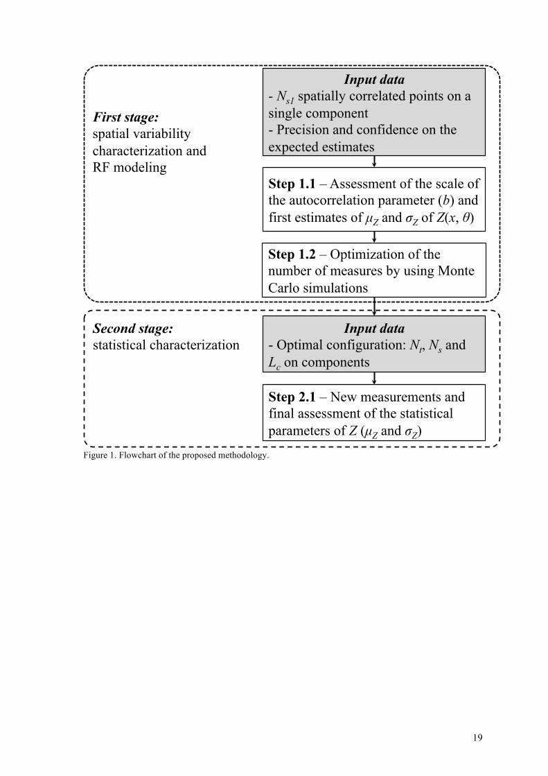
Random field theory is useful for modeling spatial variability of a given quantity (material property, deterioration process, load, etc.). Random fields could take several forms more or less complicated depending on the intrinsic characteristics of the structure (material randomness, construction process, etc.) and/or the interactions with external actions (environmental actions, deterioration processes, etc.). A stationary stochastic process can be used to represent spatial variability when the random field can be considered as homogeneous – i.e. the values of the statistical characteristics of this field do not change with the space). For instance, stationary stochastic processes have been used to model the spatial variability of surface chloride concentration [27], concrete properties [28–30] or soil properties [31–35]. In some cases, when a structure is affected by several phenomena that vary with time (e.g. deterioration) and/or with space (concrete casting in several layers), it is modeled as piecewise stationary stochastic process. This type of stochastic field can represent, for example, the vertical spatial variability of the increase of soil strength with depth or the vertical corrosion of structures located in coastal environments [10]. Figure 2 plots the mean loss of steel thickness due to corrosion with depth for sheet-piles in marine environment where the corrosion process is governed by several phenomena that depend on the exposure zone E at 10, 25 and 50 years (t10, t25 and t50). It can be observed that there is a characteristic for each considered zone –i.e., E∈[EA, ET, EL, EI, EM, ES], limited by horizontal dashed lines: from the top to the bottom, Aerial (A), Tide (T), Low level of tide (L), Immersion (I), Mud (M) and Soil (S). In this case, a piecewise stationary stochastic field could be used to have a good representation of the spatial variability of the loss of thickness.

2.2. Usual Approaches for Inspection Modeling

During inspection, there are many factors that influence the quality of measurements – e.g, environmental conditions, error in the protocol, error due to material variability, and error induced by the operator [36]. These factors could lead, for a given inspection, to under or overestimations of the measured parameter. If the parameter is underestimated, the owner could decide “do nothing” when

4

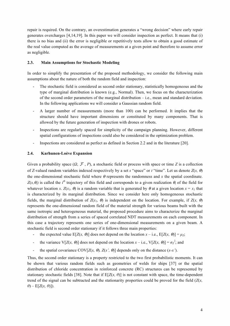
repair is required. On the contrary, an overestimation generates a “wrong decision” where early repair generates overcharges [4,14,19]. In this paper we will consider inspection as perfect. It means that (i) there is no bias and (ii) the error is negligible or repetitively tests allow to obtain a good estimate of the real value computed as the average of measurements at a given point and therefore to assume error as negligible.

2.3. Main Assumptions for Stochastic Modeling

In order to simplify the presentation of the proposed methodology, we consider the following main assumptions about the nature of both the random field and inspection:

- The stochastic field is considered as second order stationary, statistically homogeneous and the type of marginal distribution is known (e.g., Normal). Then, we focus on the characterization of the second order parameters of the marginal distribution – i.e., mean and standard deviation. In the following applications we will consider a Gaussian random field.

- A larger number of measurements (more than 100) can be performed. It implies that the structure should have important dimensions or constituted by many components. That is allowed by the future generation of inspection with drones or robots.

- Inspections are regularly spaced for simplicity of the campaign planning. However, different spatial configurations of inspections could also be considered in the optimization problem.

- Inspections are considered as perfect as defined in Section 2.2 and in the literature [20].

2.4. Karhunen-Loève Expansion

Given a probability space (Ω, F , P), a stochastic field or process with space or time Z is a collection of Z-valued random variables indexed respectively by a set s “space” or t “time”. Let us denote Z(x, θ) the one-dimensional stochastic field where θ represents the randomness and x the spatial coordinate. Z(x,θi) is called the ith trajectory of this field and corresponds to a given realization θi of the field for whatever location x. Z(x1, θ) is a random variable that is generated by θ at a given location x = x1 that is characterized by its marginal distribution. Since we consider here only homogeneous stochastic fields, the marginal distribution of Z(x1, θ) is independent on the location. For example, if Z(x, θ) represents the one-dimensional random field of the material strength for various beams built with the same isotropic and heterogeneous material, the proposed procedure aims to characterize the marginal distribution of strength from a series of spaced correlated NDT measurements on each component. In this case a trajectory represents one series of one-dimensional measurements on a given beam. A stochastic field is second order stationary if it follows three main properties:

- the expected value E[Z(x, θ)] does not depend on the location x – i.e., E[Z(x, θ)] = µZ;

- the variance V[Z(x, θ)] does not depend on the location x – i.e., V[Z(x, θ)] = σZ2; and

- the spatial covariance COV[Z(x, θ), Z(x’, θ)] depends only on the distance (x-x’).

Thus, the second order stationary is a property restricted to the two first probabilistic moments. It can be shown that various random fields such as geometries of welds for ships [37] or the spatial distribution of chloride concentration in reinforced concrete (RC) structures can be represented by stationary stochastic fields [38]. Note that if E[Z(x, θ)] is not constant with space, the time-dependent trend of the signal can be subtracted and the stationarity properties could be proved for the field (Z(x, θ) – E[Z(x, θ)]).

5

Several approaches can be used to represent a stochastic field Z(x, θ): Karhunen-Loève expansion, approximation by Fourier series, approximation EOLE, variograms, etc. [39]. In this paper, we select a Karhunen-Loève expansion to represent the stochastic field of the quantity of interest Z(x, θ) (resistance, porosity, water content, etc.). Karhunen-Loève expansion was selected by taking into account its simplicity of implementation and computational time. This expansion represents a stochastic field as a combination of orthogonal functions on a bounded interval [–a, a]:

Z(x,θ) = µZ +σZ λiξi (θ)

i=1

nkl

∑ fi (x) (1)

where, µZ is the mean of the field Z, σZ is the standard deviation of the statistically homogeneous field Z, nkl is number of terms in the truncated expansion, ξi(θ) is a set of independent centered Gaussian random variables, and λi and fi(x) are, respectively, the eigenvalues and eigenfunctions that depend on the type of autocorrelation function (ACF) ρ(Δx). It is possible to analytically determine the eigenvalues λi and eigenfunctions fi(x) for some autocorrelation functions [40]. For example, if we assume that the field is second order stationary and we consider an exponential ACF:

ρ(Δx = x1− x2 )=exp −Δx

b

⎛

⎝

⎜⎜⎜⎜⎜

⎞

⎠

⎟⎟⎟⎟⎟⎟; 0 < b

(2)

where b is the an autocorrelation parameter and Δx ∈ [–a, a]. The following transcendental eθuations can be obtained for the exponential ACF:

1b−ω tan(ωa) = 0

ω−1b

tan(ωa) = 0

⎧

⎨

⎪⎪⎪⎪⎪

⎩

⎪⎪⎪⎪⎪

(3)

where ω is obtained by solving eq. (3). If the solution of the second transcendental equation is noted ω*, the eigenfunctions are:

fi (x) =

cos(ωix)

a + sin(2ωia) / 2ωi

for even i

sin(ωi*x)

a−sin(2ωi*a) / 2ωi

* for odd i

⎧

⎨

⎪⎪⎪⎪⎪⎪⎪

⎩

⎪⎪⎪⎪⎪⎪⎪

(4)

and the corresponding eigenvalues become:

λi =

2b 1/ b2 +ωi

2( ) for even i

2b 1/ b2 +ωi

*2( ) for odd i

⎧

⎨

⎪⎪⎪⎪⎪⎪⎪

⎩

⎪⎪⎪⎪⎪⎪⎪

(5)

The spatial variability of various material properties or model parameters could be represented by an exponential autocorrelation. For instance, Figure 3 presents an autocorrelation function computed from cone penetration tests measurements in Australia [35]. It is noted that an exponential ACF as the described by eq. (2) could be used to represent the spatial autocorrelation of the measurements. The exponential ACF is adopted herein because we found that the experimental autocorrelation of the

6

spatial measures presented in section 5 follows this trend. However, other ACFs could be more appropriate to describe the spatial variability of other parameters.

3. DESCRIPTION OF THE PROPOSED METHODOLOGY

3.1. Proposed procedure

This methodology focuses on optimizing identically spaced inspections on structural components of similar characteristics – i.e., built with the same material and exposed to similar conditions. For instance, a set of 1D components (beams), or a large 1D-component subdivided artificially or physically (expansion joint or construction joints as pipe joints in a water network) in a set of short components, or belonging to a wall type structure (steel sheet pile or concrete wall). For illustrating the methodology, we consider a set of large 1D-components (beams). Section 4.4 discusses the case of small components for which characterization of spatial variability is difficult.

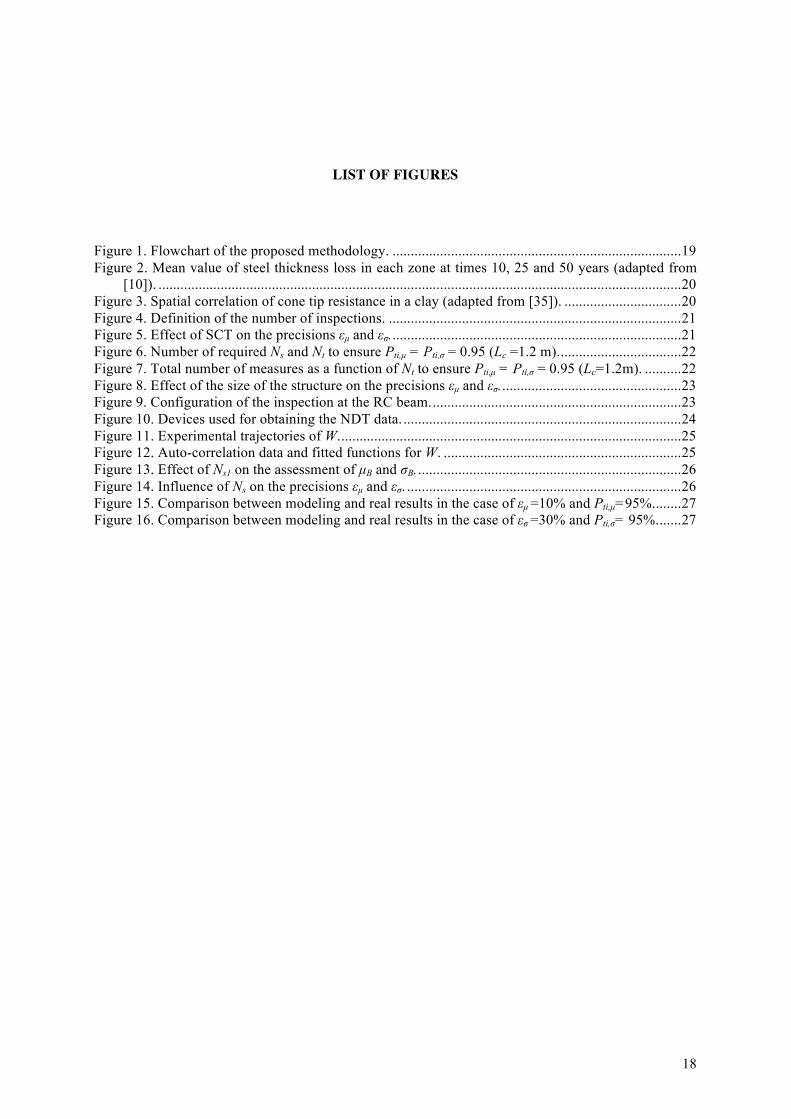
By using the results of inspections and random field modeling, we propose a two stages inspection method that provides: (i) the parameters of the spatial autocorrelation function and (ii) weakly correlated measurements that are gathered to build a sample used to characterize the statistics and the marginal distribution of Z. Figure 1 presents the flowchart of the proposed methodology.

The first stage encompasses three starts with an exhaustive inspection with Ns1 inspections closely separated at distance Lb on a single component. This exhaustive inspection aims at obtaining correlated measurements used to estimate the autocorrelation parameter b (eq. (2)). By assuming that the random field is ergodic, one trajectory is sufficient to characterize the whole joint distribution of the stochastic process. Lb is mainly defined by expert knowledge. If there is no information about Lb, a small distance could be used. It could be reduced if there is no correlated information between two consecutive measures. This stage also requires the definition of the expected precision and confidence of the estimates to characterize. The following two steps are carried out when this information is available:

Step 1.1 – Assessment of the autocorrelation parameter and first estimates of Z: the experimental autocorrelation computed by the procedure described in Section 3.2. Once b is estimated, it is possible to use eq. (2) to determine an inspection distance, Lc, which provides weakly correlated events for Z during the inspection of the components. Lb and Lc can be related by the generic term IDT for Inspection Distance Threshold. Thus, Lb and Lc should satisfy: Lb∈]0, IDT[ and Lc ∈ ]IDT, L[ where L is the length of the component. The IDT is defined by assuming that after a given distance, the events measured from an inspection can be considered as weakly correlated. A Spatial Correlation Threshold (SCT) of the spatial autocorrelation is used to determine IDT. Thus from eq. (2), the relationship between IDT and SCT is:

IDT =−bln(SCT) (6)

For instance, for b = 20cm and SCT=0.2, IDT=32.2 cm. The selection of a given SCT value will influence the parameter estimate precision. Such an aspect is illustrated in detail in section 4.2. Besides determining b, the data obtained from the inspection on the first component (weakly correlated measures) is considered to determine first estimates of the mean µZ and σZ and the standard deviation of Z. Step 1.2 – Optimization of the number of measures by using Monte Carlo simulations: the parameters b, µZ and σZ are used for modeling inspection trajectories by combining eq. (1) and

7

Monte-Carlo simulations. Each simulation simulates an inspection over a new component. Various components (whole structure) are simulated. The distance between two consecutive simulated measures for each trajectory is Lc. These simulations are devoted to determine an optimal number of inspections in terms of the precision and confidence on the estimates that are required by the asset owner (Section 3.3). Consequently, depending on the structural constraints (e.g., number and length of components) the outputs of this stage are the minimum: (i) number of components Nt, and (ii) number of inspections per component Ns separated by a distance Lc. Once Stage 1 provides an optimal configuration for new NDT inspections, Stage 2 focuses on the

statistical characterization of µZ and σZ as indicated in the following step (Figure 1): Step 2.1 – Assessment of µZ and σZ: New NDT measurements are carried out by considering the configuration provided by stage 1 (Nt, Ns and Lc). Data estimated from these weakly correlated NDT measurements is finally used to assess the statistical parameters of Z.

3.2. Assessment of the Autocorrelation Parameter from Discrete Inspections

We assume that the stationary stochastic field can be characterized by an exponential ACF that depends on a parameter b (eq. (2)) and that a trajectory is sufficient to characterize the whole joint distribution. However, the methodology can be applied to other ACF for different applications [39,41]. Let us focus on the assessment of this ACF from experimental data Z (obtained from sensors or NDT tests). Then, the autocorrelation between two observations z0 and zk, ρk is given by [34]:

ρk = i=1

nb−k

∑ zi−µZ( ) zi+k−µZ( )

i=1

nb∑ zi−µZ( )2 with 0≤ k < nb

(7)

where zi is the value of Z at location i, µZ is the mean value of Z and nb is the number of observations of Z. Two major procedures have been reported in the literature for the estimation of b for a spatially variable property from a database. The first procedure searches b that maximizes the Maximum Likelihood Estimate (MLE) [42]. The second procedure, proposed by Vanmarcke [43] and applied in [44], estimates the model parameter that provides the best fit to the sample autocorrelation. This last method can lead to a biased estimation when data is lacking. Consequently, we use the MLE for the estimation of b. Thus, the likelihood function writes:

Lh =1

2πexp −

νi2

2

⎛

⎝⎜⎜⎜⎜

⎞

⎠⎟⎟⎟⎟⎟

⎛

⎝

⎜⎜⎜⎜⎜

⎞

⎠

⎟⎟⎟⎟⎟i=1

k

∏ =1

2π

⎛

⎝⎜⎜⎜⎜

⎞

⎠⎟⎟⎟⎟

k

exp −νi

2

i=1

k

∑2

⎛

⎝

⎜⎜⎜⎜⎜⎜⎜⎜⎜⎜

⎞

⎠

⎟⎟⎟⎟⎟⎟⎟⎟⎟⎟⎟⎟

(8)

where νi is the ith component of the vector of independent standard values obtained from:

ν= C−1 Z−µZ

σZ

⎛

⎝⎜⎜⎜⎜

⎞

⎠

⎟⎟⎟⎟⎟

(9)

where Z is the vector of measurements after inspection of the random variable Z and C a lower triangular matrix such that CCT= ρ and ρ the autocorrelation matrix.

3.3. Definition of a reliability oriented measure of quality of inspection

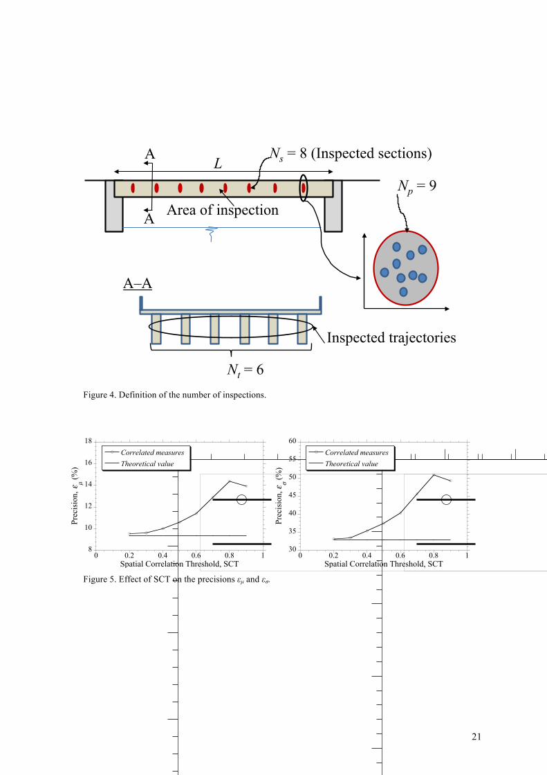
When focusing on a practical application, we aim at optimizing the total number of weakly correlated inspections N=Np×Ns×Nt where Np is the number of repetitive tests for reducing the error of inspection, Ns is the number of inspected sections and Nt the number of trajectories (Figure 4). Here,

8

the error of inspection is not considered (Section 2.3) and by neglecting the Ns1 inspections of the first stage, the total number weakly correlated inspections simply becomes N=Ns×Nt.

We use simulated data to find the minimum number of inspections that ensure a given quality of the estimates. In this case the quality will be evaluated with respect to the ‘theoretical’ expectation and standard deviation of the stochastic field Z (µZ and σZ). µZ and σZ are respectively the mean and

standard deviation of the stochastic field Z estimated from N simulated measurements after inspection and computed by:

µZ =

1N i=1

N

∑zi and σZ =1N i=1

N

∑ zi−µZ( )2 (10)

The quality of a result of inspection can be expressed by several concepts. If we consider the error of measurement, risk oriented measures have been developed: PoD, PFA [14], PoI [17], PGA and PWA [3,4]. Otherwise, and in case of a finite number of measurements and a finite size of the structure (spatial field effect), other measures can be defined based on distribution tails or a confidence interval of the probability of failure [44]. We select in this paper a confidence interval of both the mean µ and the standard deviation σ expressed as a percentage ε (precision) of µ and σ, respectively. We combine random field modeling and Monte-Carlo simulations to estimate the bounds of the confidence interval numerically for target probabilities Pti,µ and Pti,σ for both the mean and the standard deviation, respectively. In a real case, these probabilities could be defined by the asset owner depending on the type of application (structural reassessment, reliability study, etc.). These target probabilities are compared with the following probabilities computed from inspection data:

PZ

µ = P µZ ∈ (1−εµ )µZ;(1+εµ )µZ⎡⎣⎢

⎤⎦⎥( ) (11)

PZσ = P σZ ∈ (1−εσ )σZ;(1+εσ )σZ

⎡⎣⎢

⎤⎦⎥( ) (12)

Eqs (11) and (12) are very difficult to estimate. Hence, they are numerically estimated herein by considering data generated from random field modeling. If only a statistical error is considered (measures are independent), confidence intervals theory gives analytical estimates of the precision ( εµ

th

and εσth ) as a function of the number of measurements N:

εµ

th =u1−α2

σZ

µZ N (13)

εσ

th =u1−α2

12N

(14)

where u1-α/2 =1.96 for Pti,µ = Pti,σ =0.95. In the case of measurements on trajectories with a weak dependency between data, these values will increase. It is also important to note that both precision and confidence depend on the number of measurements and therefore could be limited by the structural configuration – e.g., the maximum N is limited by the structural size or the number of components.

9

Depending on the final use of the estimates, several precisions ε or confidence levels Pti can be required for the mean and the standard deviation. The optimal number of inspections can differ between these two estimates. For instance, for optimizing the assessment of µZ:

Nopt ,µ = argmin

NPti,µ ≤ PZ

µ( ) (15)

A different value Nopt,σ could be obtained for optimizing the assessment of σZ. Then, the optimal number of measurements Nopt writes:

Nopt = max Nopt ,µ ; Nopt ,σ( ) (16)

4. APPLICATION TO A NUMERICAL EXAMPLE

4.1. Problem Description

This example aims to illustrate: (i) the effect of considering correlated measures in the assessment of the mean and standard deviation of the marginal distribution, (ii) the possibilities for the selection of optimal inspection configurations for specific structures, and (iii) the special case of small size structures. We will therefore consider in the first part a structure with a larger size for which L>>b allowing to assess b from a theoretical point of view. The last part of this section highlights some issues about the size of the structures.

We suppose that the random field to inspect is Gaussian, stationary, ergodic, and characterized by: b = 1m, µZ = 100 and σZ = 20 and that the length of the structure is L=200 m. This example does not focus on the assessment of the autocorrelation parameter b. Section 5 will present a complete application of the two-stages methodology for a study case including some considerations for the assessment of b. We aim to provide an inspection protocol that ensures: Pti,µ = Pti,σ = 0.95.

4.2. Effect of SCT on the Precision of the Estimates

We first analyze the effect of the choice of SCT on the precision of the estimates quantified by εµ and εσ (Figure 5). For Ns=20 measurements on a large component (Nt=1) with length L=200m, the theoretical values computed from eqs. (13) and (14) are: εµ

th= 9.3% and εσth= 33%. These values correspond to the maximum precision estimated from N=20 independent measurements (statistical error only). It is observed that the precision obtained from consecutive measurements is close to the theoretical value when SCT is small. This effect is more pronounced when SCT is lower than 0.3 for both εµ and εσ. Therefore, it is noted that a threshold level of autocorrelation could be defined to provide the distance of inspection. In the following, we fix SCT=0.3 to compute IDT and define Lc from eq. (6).

4.3. Selection of Optimal Configurations for Inspection

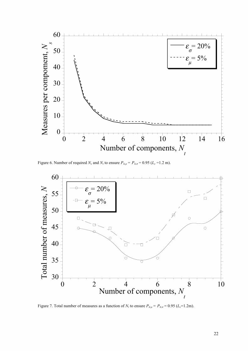
As described in Section 3.3, for given precisions (for instance εµ = 5% and εσ = 20%) and a fixed Lc value, it is possible to estimate the required number of measurements Ns and Nt to ensure Pti,µ = Pti,σ = 0.95 (eqs. (11) and (12)). By assuming that SCT=0.3, eq. (6) provides that IDT=–bln(0.3)≈1.2m. Since Lc ∈]IDT,L[, we select Lc =1.2m. Figure 6 presents the couple of minimum required values for Ns and Nt to guarantee these requirements. For both estimates, the number of measures per component

10

decreases when the number of components is larger. Based on a given structural configuration (e.g., limited number or length of components), Figure 6 illustrates how estimating the number of measures per component Ns spaced by Lc = 1.2 m on Nt components. The number of required measures is almost the same for these quality requirements. However, more measurements will be needed if we require a larger precision on the standard deviation.

The optimization can be also expressed in terms of total number or measurements N. Figure 7 gives the minimum total number of required measurements as a function of the number of available components Nt, for instance a given number of beams in a bridge. As indicated by eq. (10), there are different optimum values for the mean and the standard deviation. In this case, the optimal number of measures Nopt is driven by the assessment of µZ and computed from eq. (11). Here the optimal number is Nopt = 40 for Nt = 4 components and Ns=10 measures per component separated by Lc=1.2m. This inspection configuration requires only a total inspection zone of 12m per component. Depending on structural accessibility, the decision maker could decide to perform more spaced measurements that should improve the quality of the estimates. Different conclusions could be drawn if costs of measurements are included in the analysis. For example, the cost of inspecting an additional component could be higher than the cost of increasing the number of measures per component.

4.4. Effect of the Size of the Structure

Previous subsections assume that the components are larger enough to find a set of “weakly correlated” measurements. Let us focus on small structures and the related shortcomings for optimal characterization. We consider the same stochastic field as described in Section 4.1 and we decrease the size of a structure from the original length of 200m until 10m. Figure 8 shows the effect of the size of the structure on the precision of the estimates µZ and σZ. These results correspond to N=20 measures on a single component. Therefore, the theoretical precisions agree with the values computed in Section 4.2. When SCT>0.8, there is no a unique trend because in this case the measures are very close and only describe the local shape of the inspected trajectory. For components larger than 50m, 20 measurements can be realized whatever SCT. It is consequently observed that for L>50m both εµ and εσ converge similarly to the case where L=200m (Figure 5). It is also noted that for shorter components (L=10 and 25m) the values of εµ and εσ cannot be computed because it is not possible to carry out 20 measures. Therefore, the convergence until the theoretical value cannot be reached for shorter components. For shorter components, the precision on the assessment of the estimates µZ and σZ could be improved by adding more measurements on additional components Nt>1. However, if L<b, it could be very difficult to obtain a good characterization of the spatial variability.

5. APPLICATION TO A STUDY CASE

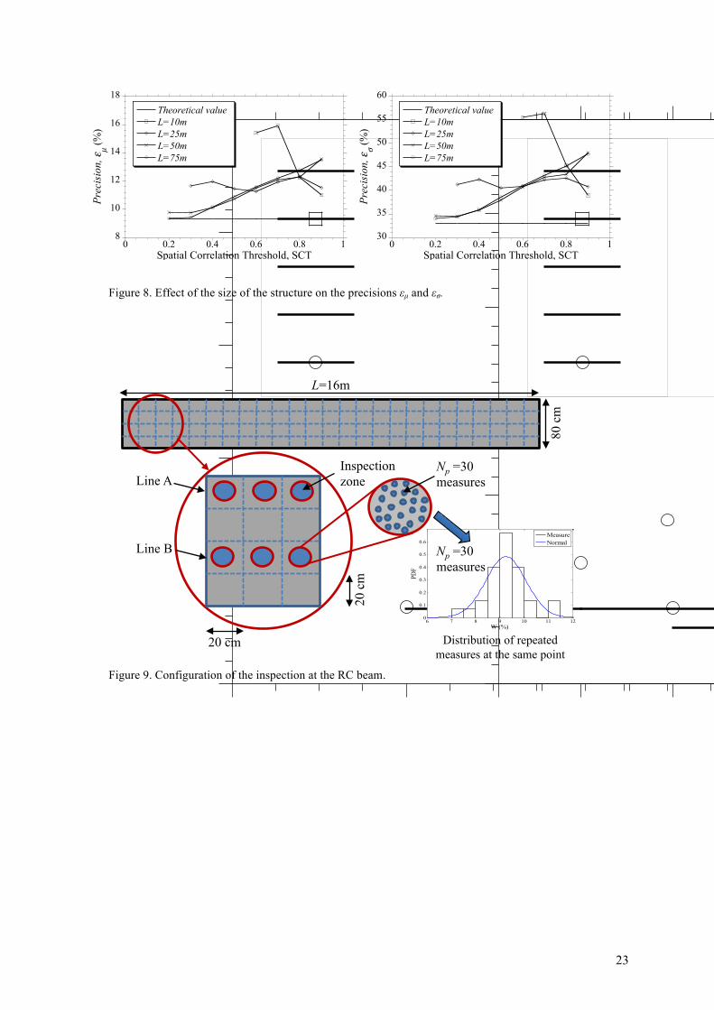
5.1. Description of the Structure and the NDT Tool

The objective of this example is to characterize the marginal distribution and spatial variability of the water content W, modeled as a second order random variable, for a reinforced concrete beam exposed to natural environmental conditions in Bouguenais (Pays de la Loire, France) by using NDT inspections (Capacitive technique). The inspection was performed on the first of March 2012 with high relative humidity of air (Hair=99%) and a low temperature (T=5°C). Figure 9 presents the configuration of the experiment. The proposed methodology is applied to inspections on two

11

horizontal trajectories called Line A and Line B. A vertical distance of 40 cm separates these lines. To neglect the error of the measurement, we performed Np=30 repetitive tests on each point and we select the mean value to represent the reference measurement of water content at each point. Figure 9 also includes the histogram for these Np=30 repetitive tests. Therefore, according to Section 2.2, we justify the assumption that these repetitive tests will provide a “perfect” measurement. The repetitive tests are carried out on Ns=80 horizontal points separated by 20 cm for each line.

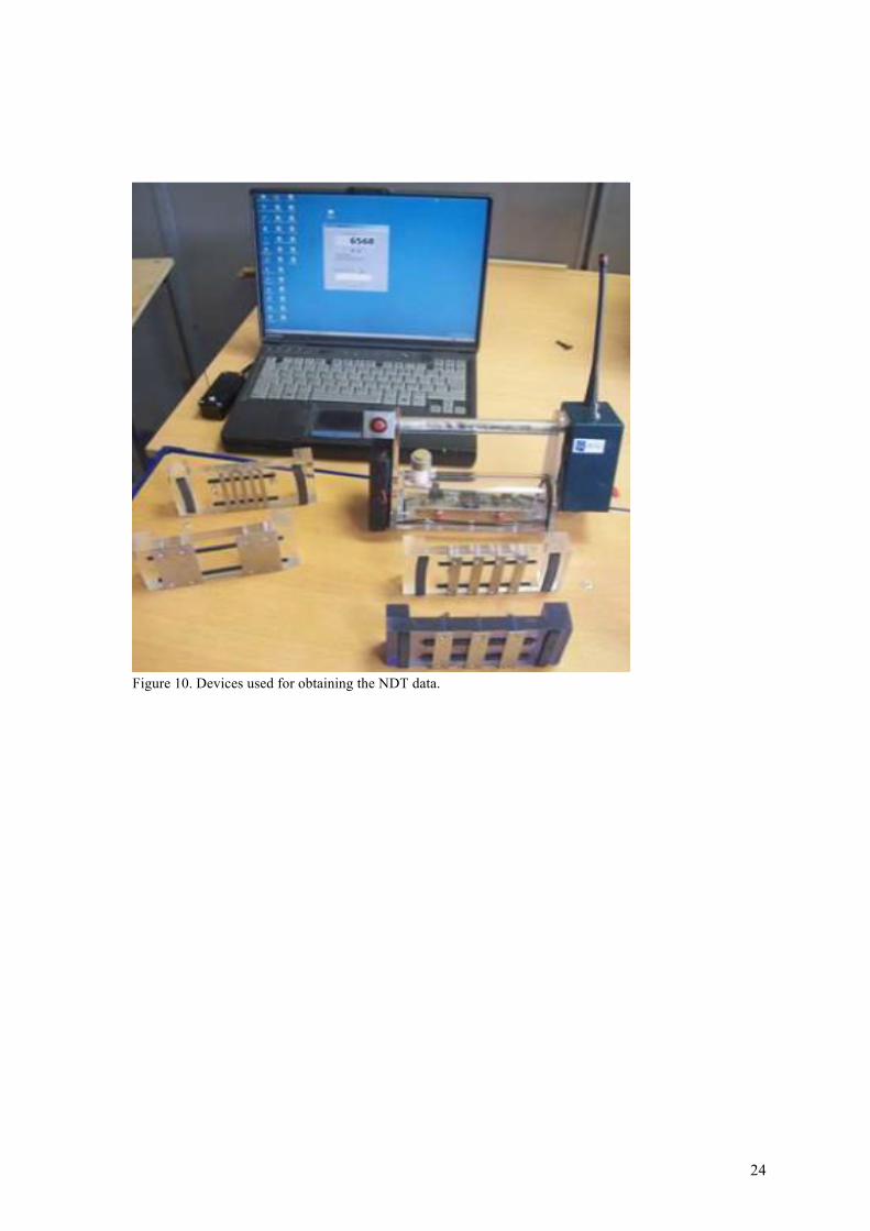
Figure 10 presents the experimental devices. The principle of the Capacitive technique is based on the resonance frequency measurement of an oscillating circuit (around 30-35 MHz) between several electrodes lying on the upper face of the concrete slab (Figure 9) [45,46]. As the combination of medium and electrodes behave like a capacitor, a variation of the dielectric properties of the medium induces a shift of the resonant frequency. A calibration enables to obtain directly the concrete relative permittivity from the frequency measurements, which is mainly related to the water content and the mixing components [47–49]. The volume investigated depends on the geometry of the electrodes. In this study, we used larger electrodes to investigate a 6-8 cm depth of concrete, volume that is more coherent with ground penetrating radar measurements. For simplicity, we consider, for this concrete, a linear relationship between relative humidity and NDT outputs:

W =

48.4981−(Fc−Fair )31.753

(17)

where Fc and Fair are frequency values in RC beam and in the air at situ, respectively. Ongoing studies in several laboratories worldwide are searching for more accurate relationships by considering a multi-technique approach to account that each NDT tool is sensitive to humidity, porosity, size and type of aggregates.

5.2. Data and Modeling

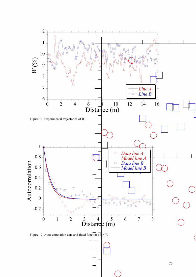
Figure 11 presents the two trajectories obtained for lines A and B based on measures with a filter that remove the few outliers. The shape and the values are different for each line. Line A shows more variability but lower values in comparison to line B. It is expected to find lower water content in the line A because the drying process is faster in the upper zones – i.e., they are more exposed to wind and there is a diffusion of water through the lower zones. The variability could also be explained by other factors as the segregation of concrete. Taking into account this variability with height, we cannot merge the data of both lines to estimate the marginal distribution of W in this practical application. Therefore, in this case we will use the data from one trajectory to characterize the spatial variability and recommend an optimal number and spatial distribution of measures for the second trajectory. We verify first that the autocorrelation shape is similar.

Figure 12 presents the autocorrelation data for trajectories A and B. We obtained a classical shape where the autocorrelation decreases with distance including negative values [34]. After fitting the experimental data with eq. (2) according to the method presented in Section 3.2, we found that the exponential autocorrelation functions are very close for the two lines. We obtained: b=0.45m and b=0.51m for lines A and B, respectively. It means that the exponential function could be useful to represent the autocorrelation and therefore for modeling the horizontal spatial variability of the water content in RC beams at different depths. Data of line B seems to be more regular (Figure 11) and its experimental autocorrelation is more close to the exponential function. Therefore, in the following, we will use the data from line B to characterize the spatial variability and recommend an optimal number and spatial distribution of measures for the study of the data of line A. Figure 12 only presents

12

autocorrelation values for 8m to illustrate the decay of the values for the first 2 meters; but these values were estimated by considering the information of the whole beam (16m).

5.3. First Stage

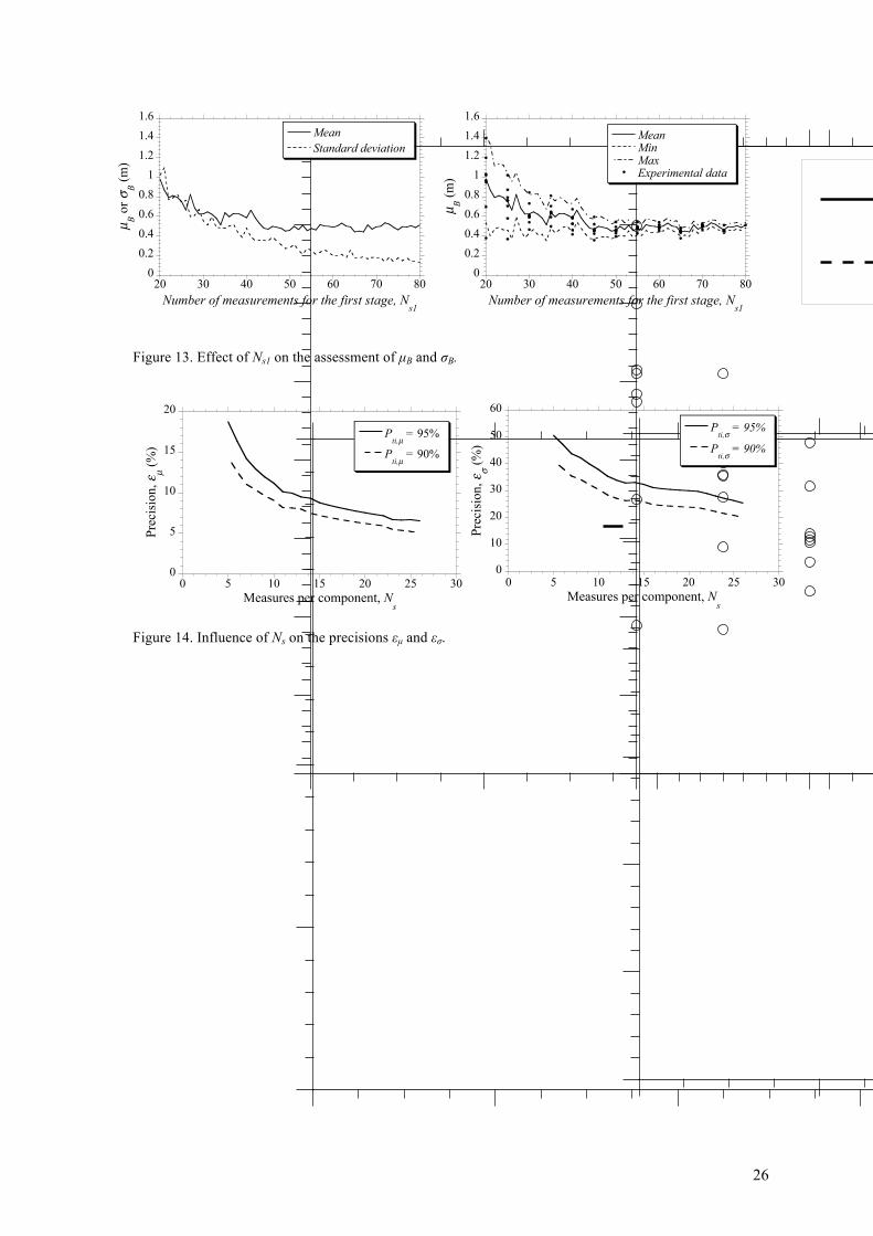
According to Section 3, the first stage of the inspection methodology is devoted to the assessment of b on a single trajectory. There is an error on the assessment of b because this parameter is deduced from a limited number of measurements Ns1 on a given trajectory. This error is mainly due to the number of measurements Ns1 on a trajectory (statistical error) and the choice of Lb. Although b could be modeled as a random variable B, we decide to consider it as a deterministic value determined from sufficiently correlated measures. b for line B is b=0.51m. Thus, we validate that the inspection distance Lb = 0.2m ensures higher correlation between measured data (Figure 12). By defining a SCT=0.3, we can determine IDT=0.61m from eq. (6). Then the distance between two weakly correlated inspections is Lc =0.6 m for determining the first estimates of µZ and σZ that will be used to model the random field. By using the experimental data obtained from this first stage, Figure 13a plots µB and σB as a function of the number of measures in the first trajectory Ns1 for 1,000 simulated trajectories. The convergence of µB through the value of b determined from the 80 measurements is faster and the error is less than 0.05m for Ns1 ≥ 45 measures. σB decreases when Ns1 is larger by reducing the uncertainty on the assessment of the parameter b.

Figure 13b presents the mean and the 95% confidence interval of µB for 1000 simulated trajectories as well as the values of b computed from experimental data, as a function of Ns1. The various experimental points for a given Ns1 correspond to different sets of Ns1 over the total number of measurements. It can be observed that the scatter is large when Ns1 decreases and could even reach 0.9m for Ns1=20. It is also noted that b estimated from experimental data is close to µB when Ns1>45. These results therefore indicate that the assessment of b requires a minimum number of correlated measures Ns1.

Let us now fix the value Ns1=45 measures and optimize the number and spatial distribution of measurements. By considering the autocorrelation parameter identified during the first stage (b=0.51m) and selecting a SCT=0.3, the distance between two weakly correlated inspections is Lc =0.6 m. Due to the length of the beam, practically, the maximum number of measures is max(Ns,)= 26. This information is used to estimate the theoretical mean and standard deviation from weakly correlated measures µW,26=10.12% σW,26=0.67%. Values of µW,26, σW,26 and b will be used to optimize the number and spatial distribution of inspections.

Figure 14 describes the effect of the choice of a confidence level (Pti =95% and 90%) on the precisions εµ and εσ. After performing Monte Carlo simulations, we plot the evolution of εµ and εσ as a function of the number of measures per trajectory Ns. The shape of the curves is consistent with the theoretical eqs. (13) and (14). Namely, εµ and εσ decrease for larger quantity of available data. For all cases, more inspections are required if the confidence level increases. For example, at a given precision level εµ =10%, the needed number of inspections Ns increases from 9 to 12 if the confidence level increases from 90% to 95%. It is also noted that the maximum precisions are limited by the geometry of the structure in this case. For instance, for a confidence level of 90%, the maximum precisions are εµ =5.2% and εσ =20% when Ns =26 measures.

For the second stage, we fix the following precision levels (εµ =10% and εσ =30%) and the confidence interval (Pti,µ = Pti,σ=95%). Consequently, by using the results presented in Figure 14, we obtain the optimum values: Nopt,µ=12 and Nopt,σ=20 measures. Finally, by applying eq. (15), Nopt=20 measures. This information will be used to characterize the marginal distribution of the water content on the line A, modeled as a second order variable.

13

5.4. Second Stage and Validation

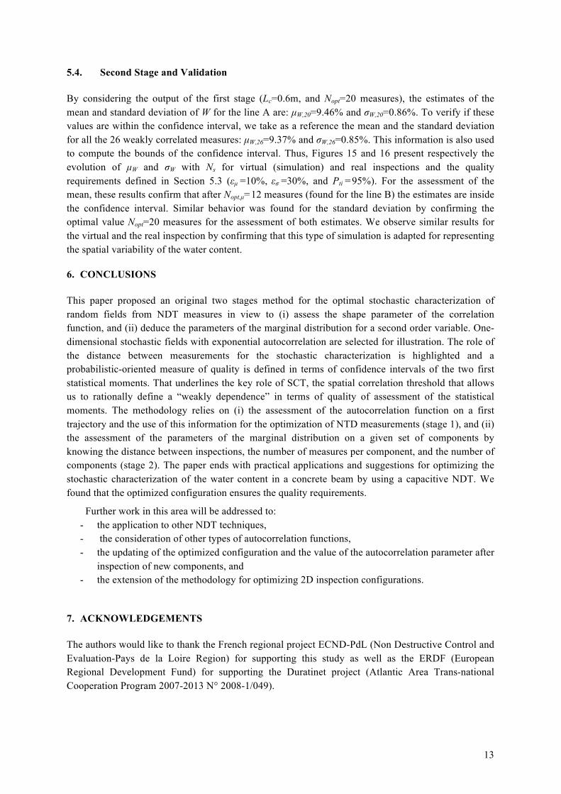
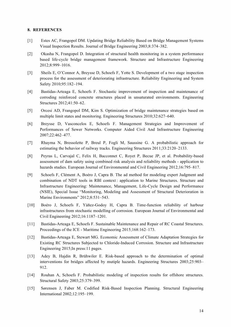
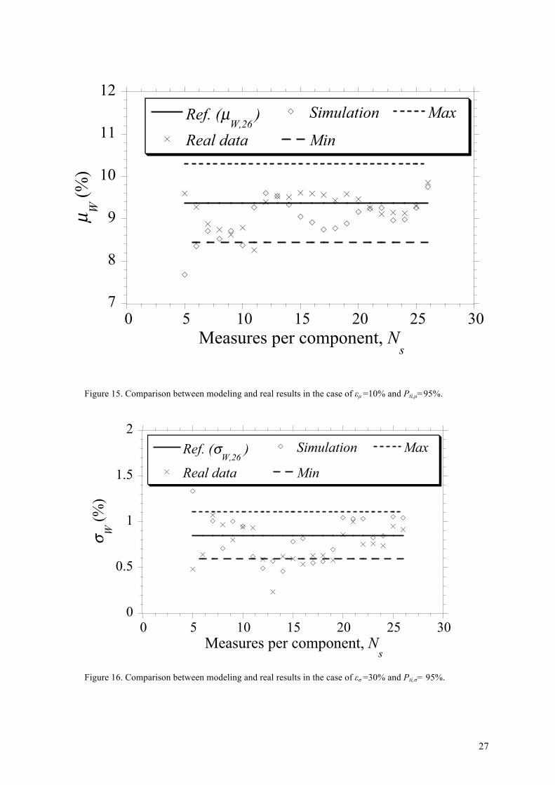
By considering the output of the first stage (Lc=0.6m, and Nopt=20 measures), the estimates of the mean and standard deviation of W for the line A are: µW,20=9.46% and σW,20=0.86%. To verify if these values are within the confidence interval, we take as a reference the mean and the standard deviation for all the 26 weakly correlated measures: µW,26=9.37% and σW,26=0.85%. This information is also used to compute the bounds of the confidence interval. Thus, Figures 15 and 16 present respectively the evolution of µW and σW with Ns for virtual (simulation) and real inspections and the quality requirements defined in Section 5.3 (εµ =10%, εσ =30%, and Pti =95%). For the assessment of the mean, these results confirm that after Nopt,µ=12 measures (found for the line B) the estimates are inside the confidence interval. Similar behavior was found for the standard deviation by confirming the optimal value Nopt=20 measures for the assessment of both estimates. We observe similar results for the virtual and the real inspection by confirming that this type of simulation is adapted for representing the spatial variability of the water content.

6. CONCLUSIONS

This paper proposed an original two stages method for the optimal stochastic characterization of random fields from NDT measures in view to (i) assess the shape parameter of the correlation function, and (ii) deduce the parameters of the marginal distribution for a second order variable. One-dimensional stochastic fields with exponential autocorrelation are selected for illustration. The role of the distance between measurements for the stochastic characterization is highlighted and a probabilistic-oriented measure of quality is defined in terms of confidence intervals of the two first statistical moments. That underlines the key role of SCT, the spatial correlation threshold that allows us to rationally define a “weakly dependence” in terms of quality of assessment of the statistical moments. The methodology relies on (i) the assessment of the autocorrelation function on a first trajectory and the use of this information for the optimization of NTD measurements (stage 1), and (ii) the assessment of the parameters of the marginal distribution on a given set of components by knowing the distance between inspections, the number of measures per component, and the number of components (stage 2). The paper ends with practical applications and suggestions for optimizing the stochastic characterization of the water content in a concrete beam by using a capacitive NDT. We found that the optimized configuration ensures the quality requirements.

Further work in this area will be addressed to: - the application to other NDT techniques, - the consideration of other types of autocorrelation functions, - the updating of the optimized configuration and the value of the autocorrelation parameter after

inspection of new components, and - the extension of the methodology for optimizing 2D inspection configurations.

7. ACKNOWLEDGEMENTS

The authors would like to thank the French regional project ECND-PdL (Non Destructive Control and Evaluation-Pays de la Loire Region) for supporting this study as well as the ERDF (European Regional Development Fund) for supporting the Duratinet project (Atlantic Area Trans-national Cooperation Program 2007-2013 N° 2008-1/049).

14

8. REFERENCES

[1] Estes AC, Frangopol DM. Updating Bridge Reliability Based on Bridge Management Systems Visual Inspection Results. Journal of Bridge Engineering 2003;8:374–382.

[2] Okasha N, Frangopol D. Integration of structural health monitoring in a system performance based life-cycle bridge management framework. Structure and Infrastructure Engineering 2012;8:999–1016.

[3] Sheils E, O’Connor A, Breysse D, Schoefs F, Yotte S. Development of a two stage inspection process for the assessment of deteriorating infrastructure. Reliability Engineering and System Safety 2010;95:182–194.

[4] Bastidas-Arteaga E, Schoefs F. Stochastic improvement of inspection and maintenance of corroding reinforced concrete structures placed in unsaturated environments. Engineering Structures 2012;41:50–62.

[5] Orcesi AD, Frangopol DM, Kim S. Optimization of bridge maintenance strategies based on multiple limit states and monitoring. Engineering Structures 2010;32:627–640.

[6] Breysse D, Vasconcelos E, Schoefs F. Management Strategies and Improvement of Performances of Sewer Networks. Computer Aided Civil And Infrastructure Engineering 2007;22:462–477.

[7] Rhayma N, Bressolette P, Breul P, Fogli M, Saussine G. A probabilistic approach for estimating the behavior of railway tracks. Engineering Structures 2011;33:2120–2133.

[8] Peyras L, Carvajal C, Felix H, Bacconnet C, Royet P, Becue JP, et al. Probability-based assessment of dam safety using combined risk analysis and reliability methods - application to hazards studies. European Journal of Environmental and Civil Engineering 2012;16:795–817.

[9] Schoefs F, Clément A, Boéro J, Capra B. The ad method for modeling expert Judgment and combination of NDT tools in RBI context : application to Marine Structures. Structure and Infrastructure Engineering: Maintenance, Management, Life-Cycle Design and Performance (NSIE), Special Issue “Monitoring, Modeling and Assessment of Structural Deterioration in Marine Environments” 2012;8:531–543.

[10] Boéro J, Schoefs F, Yáñez-Godoy H, Capra B. Time-function reliability of harbour infrastructures from stochastic modelling of corrosion. European Journal of Environmental and Civil Engineering 2012;16:1187–1201.

[11] Bastidas-Arteaga E, Schoefs F. Sustainable Maintenance and Repair of RC Coastal Structures. Proceedings of the ICE - Maritime Engineering 2015;168:162–173.

[12] Bastidas-Arteaga E, Stewart MG. Economic Assessment of Climate Adaptation Strategies for Existing RC Structures Subjected to Chloride-Induced Corrosion. Structure and Infrastructure Engineering 2015;In press:11 pages.

[13] Adey B, Hajdin R, Brühwiler E. Risk-based approach to the determination of optimal interventions for bridges affected by mutiple hazards. Engineering Structures 2003;25:903–912.

[14] Rouhan A, Schoefs F. Probabilistic modeling of inspection results for offshore structures. Structural Safety 2003;25:379–399.

[15] Sørensen J, Faber M. Codified Risk-Based Inspection Planning. Structural Engineering International 2002;12:195–199.

15

[16] Stewart MG, Mullard JA. Spatial time-dependent reliability analysis of corrosion damage and the timing of first repair for RC structures. Engineering Structures 2007;29:1457–1464.

[17] Straub D, Faber MH. Modelling dependency in inspection performance, in: M. Der Kiureghian, Pestana (Eds.), Application of Statistics and Probability in Civil Engineering, ICASP, San Franncisco, USA: 2003: pp. 1123–1130.

[18] Faber M. Risk Based Inspection: The Framework. Structural Engineering International 2002;12:186–194.

[19] Sheils E, O’Connor A, Schoefs F, Breysse D. Investigation of the effect of the quality of inspection techniques on the optimal inspection interval for structures. Structure and Infrastructure Engineering 2012;8:557–568.

[20] Schoefs F, Clement A, Nouy A. Assessment of spatially dependent ROC curves for inspection of random fields of defects. Structural Safety 2009;31:409–419.

[21] Beck JL, Katafygiotis LS. Updating Models and Their Uncertainties: Bayesian Statistical Framework. Journal of Engineering Mechanics 1998;124:455–461.

[22] Tran T-B, Bastidas-Arteaga E, Schoefs F. Improved Bayesian network configurations for probabilistic identification of degradation mechanisms: application to chloride ingress. Structure and Infrastructure Engineering 2015;1–15.

[23] Lu L, Chekroun M, Abraham O, Maupin V, Villain G. Mechanical properties estimation of functionally graded materials using surface waves recorded with a laser interferometer. NDT & E International 2011;44:169–177.

[24] Nguyen NT, Sbartaï Z-M, Lataste J-F, Breysse D, Bos F. Assessing the spatial variability of concrete structures using NDT techniques – Laboratory tests and case study. Construction and Building Materials 2013;49:240–250.

[25] Nguyen NT, Sbartaï ZM, Lataste J-F, Breysse D, Bos F. Non-destructive evaluation of the spatial variability of reinforced concrete structures. Mechanics & Industry 2014;16:103.

[26] Gomez-Cardenas C, Sbartaï ZM, Balayssac JP, Garnier V, Breysse D. New optimization algorithm for optimal spatial sampling during non-destructive testing of concrete structures. Engineering Structures 2015;88:92–99.

[27] O’Connor A, Kenshel O. Experimental Evaluation of the Scale of Fluctuation for Spatial Variability Modeling of Chloride-Induced Reinforced Concrete Corrosion. Journal Of Bridge Engineering 2013;18:3–14.

[28] Bazant Z, Xi Y. Statistical Size Effect in Quasi-brittle Structures: II. Nonlocal Theory. ASCE J. of Engrg. Mech. 1991;117:2623–2640.

[29] Bazant Z, Novák D. Probabilistic Nonlocal Theory for Quasibrittle Fracture Initiation and Size Effect. I: Theory. Journal of Engineering Mechanics 2000;126:166–174.

[30] Bazant Z, Novák D. Probabilistic Nonlocal Theory for Quasibrittle Fracture Initiation and Size Effect. II: Application. Journal of Engineering Mechanics 2000;126:175–185.

[31] Srivastava A. Spatial Variability Modelling of Geotechnical Parameters and Stability of Highly Weathered Rock Slope. Indian Geotechnical Journal 2012;42:179–185.

[32] Nobahar A. Effects of soil spatial variability on soil-structure interaction, PhD Thesis, Memorial University, St. John’s, NL., 2003.

[33] Griffiths DV, Fenton GA. Influence of soil strength spatial variability on the stability of an

16

undrained clay slope by finite elements. Slope Stability 2000. ASCE 2000;184–193.

[34] Chenari RJ, Dodaran RO. New method for estimation of the scale of fluctuation of geotechnical properties in natural deposits. Computational Methods in Civil Engineering 2010;1:55–66.

[35] Jaksa MB, Kaggwa WS, Brooker PI. Experimental evaluation of the scale of fluctuation of a stiff clay, in: Application of Stochastics and Probability, Melcher an, Sydney Balkema, Rotterdam: 2000: pp. 415–422.

[36] Breysse D, Yotte S, Salta M, Schoefs F, Ricardo J, Chaplain M. Accounting for variability and uncertainties in NDT condition assessment of corroded RC structures. European Journal of Environmental and Civil Engineering 2009;13:573–592.

[37] Pasqualini O, Schoefs F, Chevreuil M, Cazuguel M. Measurements and statistical analysis of fillet weld geometrical parameters for probabilistic modelling of the fatigue capacity. Marine Structures 2013;34:226–248.

[38] Schoefs F, Yáñez-Godoy H, Lanata F. Polynomial chaos representation for identification of mechanical characteristics of instrumented structures. Computer-Aided Civil and Infrastructure Engineering 2011;26:173–189.

[39] Li C-C, Der Kiureghian A. Optimal discretization of random fields. J Eng Mech ASCE 1993;119:1136–1154.

[40] Ghanem R, Spanos RD. Stochastic Finite Elements - A Spectral Approach. New York, USA: Springer, 2003.

[41] Kenshel O. Influence of spatial variability on whole life management of reinforced concrete bridges, University of Dublin, Trinity College, Dublin, Ireland, 2009.

[42] Li Y. Effect of spatial variability on maintenance and repair decisions for concrete structures, Delft University, Delft, Netherlands, 2004.

[43] Vanmarcke E. Random fields: analysis and synthesis. Mass, London: MIT Press, Cambridge, 1983.

[44] Schoefs F, Tran TV, Bastidas-Arteaga E. Optimization of inspection and monitoring of structures in case of spatial fields of deterioration/properties, in: ICASP -Applications of Statistics and Probability in Civil Engineering, Zurïch: Taylor & Francis Group, ISBN 978-0-415-66986-3., 2011.

[45] Dérobert X, Iaquinta J, Klysz G, Balayssac JP. Use of capacitive and GPR techniques for non-destructive evaluation of cover concrete. NDT&E International. 2008;41:44–52.

[46] Villain G, Sbartaï ZM, Dérobert X, Garnier V, Balayssac JP. Durability diagnosis of a concrete structure in a tidal zone by combining NDT methods: Laboratory tests and case study. Construction and Building Materials 2012;37:893–903.

[47] Robert A. Dielectric permittivity of concrete between 50 MHz and 1 GHz and GPR measurements for building materials evaluation. Journal of Applied Geophysics 1998;40:89–94.

[48] Soutsos MN, Bungey JH, Millard SG, Shaw MR, Patterson A. Dielectric properties of concrete and their influence on radar testing. NDT & E International 2001;34:419–425.

[49] Dérobert X, Villain G, Cortas R, Chazelas JL. EM characterization of hydraulic concretes in the GPR frequencyband using a quadratic experimental design NDT, in: 7th Int. Symposium on

17

Non-Destructive Testing in Civil Engineering NDTCE’09, Nantes, France: 2009: pp. 177–182.

18

LIST OF FIGURES

Figure 1. Flowchart of the proposed methodology. ............................................................................... 19Figure 2. Mean value of steel thickness loss in each zone at times 10, 25 and 50 years (adapted from

[10]). ............................................................................................................................................... 20Figure 3. Spatial correlation of cone tip resistance in a clay (adapted from [35]). ................................ 20Figure 4. Definition of the number of inspections. ................................................................................ 21Figure 5. Effect of SCT on the precisions εµ and εσ. ............................................................................... 21Figure 6. Number of required Ns and Nt to ensure Pti,µ = Pti,σ = 0.95 (Lc =1.2 m). ................................. 22Figure 7. Total number of measures as a function of Nt to ensure Pti,µ = Pti,σ = 0.95 (Lc=1.2m). .......... 22Figure 8. Effect of the size of the structure on the precisions εµ and εσ. ................................................. 23Figure 9. Configuration of the inspection at the RC beam. .................................................................... 23Figure 10. Devices used for obtaining the NDT data. ............................................................................ 24Figure 11. Experimental trajectories of W. ............................................................................................. 25Figure 12. Auto-correlation data and fitted functions for W. ................................................................. 25Figure 13. Effect of Ns1 on the assessment of µB and σB. ........................................................................ 26Figure 14. Influence of Ns on the precisions εµ and εσ. ........................................................................... 26Figure 15. Comparison between modeling and real results in the case of εµ =10% and Pti,µ=95%. ....... 27Figure 16. Comparison between modeling and real results in the case of εσ =30% and Pti,σ= 95%. ...... 27

19

First stage: spatial variability characterization and RF modeling

Second stage: statistical characterization

Step 1.1 – Assessment of the scale of the autocorrelation parameter (b) and first estimates of µZ and σZ of Z(x, θ)

Input data - Ns1 spatially correlated points on a single component - Precision and confidence on the expected estimates

Input data - Optimal configuration: Nt, Ns and Lc on components

Step 2.1 – New measurements and final assessment of the statistical parameters of Z (µZ and σZ)

Step 1.2 – Optimization of the number of measures by using Monte Carlo simulations

Figure 1. Flowchart of the proposed methodology.

20

-16

-14

-12

-10

-8

-6

-4

-2

0

0 1 2 3 4 5

Dep

th (m

)

Loss of thickness (mm)

t10 t25 t50

ET

EL

EI

EM

ES

EA

Figure 2. Mean value of steel thickness loss in each zone at times 10, 25 and 50 years (adapted from [10]).

Figure 3. Spatial correlation of cone tip resistance in a clay (adapted from [35]).

21

L

Area of inspection

Inspected trajectories

A

A

A–A

Nt = 6

Ns = 8 (Inspected sections)

Np = 9

Figure 4. Definition of the number of inspections.

8

10

12

14

16

18

0 0.2 0.4 0.6 0.8 1

Correlated measuresTheoretical value

Prec

isio

n, ε µ (%

)

Spatial Correlation Threshold, SCT

30

35

40

45

50

55

60

0 0.2 0.4 0.6 0.8 1

Correlated measuresTheoretical value

Prec

isio

n, εσ (%

)

Spatial Correlation Threshold, SCT Figure 5. Effect of SCT on the precisions εµ and εσ.

22

0

10

20

30

40

50

60

0 2 4 6 8 10 12 14 16

εσ= 20%

εµ= 5%

Mea

sure

s pe

r com

pom

ent,

Ns

Number of components, Nt

Figure 6. Number of required Ns and Nt to ensure Pti,µ = Pti,σ = 0.95 (Lc =1.2 m).

30

35

40

45

50

55

60

0 2 4 6 8 10

εσ= 20%

εµ= 5%

Tota

l num

ber o

f mea

sure

s, N

Number of components, Nt

Figure 7. Total number of measures as a function of Nt to ensure Pti,µ = Pti,σ = 0.95 (Lc=1.2m).

23

8

10

12

14

16

18

0 0.2 0.4 0.6 0.8 1

Theoretical valueL=10mL=25mL=50mL=75m

Prec

isio

n, εµ (%

)

Spatial Correlation Threshold, SCT

30

35

40

45

50

55

60

0 0.2 0.4 0.6 0.8 1

Theoretical valueL=10mL=25mL=50mL=75m

Prec

isio

n, εσ (%

)

Spatial Correlation Threshold, SCT

Figure 8. Effect of the size of the structure on the precisions εµ and εσ.

L=16m

Inspection zone

Line A

Line B

20 cm

20 c

m

80 c

m

Np =30 measures

6 7 8 9 10 11 120

0.1

0.2

0.3

0.4

0.5

0.6

W (%)

PDF

MeasureNormal

Np =30 measures

Distribution of repeated measures at the same point

Figure 9. Configuration of the inspection at the RC beam.

24

Figure 10. Devices used for obtaining the NDT data.

25

6

7

8

9

10

11

12

0 2 4 6 8 10 12 14 16

Line ALine B

W (%

)

Distance (m)

Figure 11. Experimental trajectories of W.

-0.2

0

0.2

0.4

0.6

0.8

1

0 1 2 3 4 5 6 7 8

Data line AModel line AData line BModel line B

Aut

ocor

rela

tion

Distance (m)

Figure 12. Auto-correlation data and fitted functions for W.

26

0

0.2

0.4

0.6

0.8

1

1.2

1.4

1.6

20 30 40 50 60 70 80

MeanStandard deviation

µ B or σ

B (m)

Number of measurements for the first stage, Ns1

0

0.2

0.4

0.6

0.8

1

1.2

1.4

1.6

20 30 40 50 60 70 80

MeanMinMaxExperimental data

µ B (m)

Number of measurements for the first stage, Ns1

Figure 13. Effect of Ns1 on the assessment of µB and σB.

0

5

10

15

20

0 5 10 15 20 25 30

Pti,µ

= 95%

Pti,µ

= 90%

Prec

isio

n, εµ (%

)

Measures per component, Ns

0

10

20

30

40

50

60

0 5 10 15 20 25 30

Pti,σ

= 95%

Pti,σ

= 90%

Prec

isio

n, εσ (%

)

Measures per component, Ns

Figure 14. Influence of Ns on the precisions εµ and εσ.

27

7

8

9

10

11

12

0 5 10 15 20 25 30

Ref. (µW,26

)

Real data

Simulation

Min

Max

µ W (%

)

Measures per component, Ns

Figure 15. Comparison between modeling and real results in the case of εµ =10% and Pti,µ=95%.

0

0.5

1

1.5

2

0 5 10 15 20 25 30

Ref. (σW,26

)

Real data

Simulation

Min

Max

σ W (%

)

Measures per component, Ns

Figure 16. Comparison between modeling and real results in the case of εσ =30% and Pti,σ= 95%.