Characterization of pharmaceutical powder blends usingin situ near-infrared chemical imaging

Juan G. Osorio a, Gina Stuessy b, Gabor J. Kemeny b, Fernando J. Muzzio a,n

a Department of Chemical and Biochemical Engineering, Rutgers University, 98 Brett Road, Piscataway, NJ 08854, USAb Middleton Research, 8505 University Green, Middleton, WI 53562, USA

H I G H L I G H T S

� Composition maps of each materialin a powder blend measured forselected rotations.

� Automated chemical image analysisparameters were measured to studyblending dynamics.

� Large acetaminophen aggregateswere observed even after 190 turnsin low-shear blending.

� In all blends, Avicel blendedsignificantly more slowly than lactose.

� Increase in acetaminophen concentra-tion slowed the blending of otherexcipients.

G R A P H I C A L A B S T R A C T

a r t i c l e i n f o

Article history:Received 31 August 2013Received in revised form22 November 2013Accepted 17 December 2013Available online 18 January 2014

Keywords:PowdersMixingPharmaceuticalsParticulate processesMicro-mixingNIR chemical imaging

a b s t r a c t

The present study introduces a new in situ near-infrared chemical imaging technique (imMixTM)designed to characterize micro-mixing in pharmaceutical powder blends. The technique uses in-line,non-contact monitoring of the blending process, eliminating the bias introduced by commonly usedpowder sampling techniques. A Science-Based Calibration (SBC) chemometric method, which uses purecomponent spectral data to create a calibration model, was used to create concentration maps of theblends studied here. The advantage of SBC over the alternative Partial Least Squares (PLS) or PrincipalComponent Analysis (PCA) calibration methods is that it does not require a large number of samples tocreate a calibration. The imMix system proved to be useful in monitoring the spatial distribution andaggregate sizes of acetaminophen, used as the model drug, and of excipients in the blends. Using a 1-lbin-blender, measurements were able to detect changes in the constituents and other experimentalparameters as a function of blending time. Such measurements can be used to determine the mixingtime and shear requirements of blends during product and process development.

& 2013 Elsevier Ltd. All rights reserved.

1. Introduction

Batch powder mixing is one of the most common and impor-tant unit operations in a wide range of industries, such as food,cosmetics, pharmaceuticals, chemicals, ceramics, and catalysts. Inpharmaceuticals, it has been the focus of intense interest in thepast 20 years, and it has been the subject of many studies. Most ofthe research has focused on characterizing the process for a given

Contents lists available at ScienceDirect

journal homepage: www.elsevier.com/locate/ces

Chemical Engineering Science

0009-2509/$ - see front matter & 2013 Elsevier Ltd. All rights reserved.http://dx.doi.org/10.1016/j.ces.2013.12.027

n Corresponding author. Tel.: þ1 732 445 3357.E-mail addresses: josorio@eden.rutgers.edu (J.G. Osorio),

gina@middletonresearch.com (G. Stuessy),gabor@middletonresearch.com (G.J. Kemeny), fjmuzzio@yahoo.com (F.J. Muzzio).

Chemical Engineering Science 108 (2014) 244–257

set of materials and determining the design parameters that willreach the required blend homogeneity. Quantification of mixingefficiency has concentrated on characterizing the bulk homoge-neity of the relevant constituents, primarily the active pharma-ceutical ingredients (APIs) and, to a lesser extent, other functionalingredients such as lubricants, glidants, and disintegrants inpowder blends. Studies have been carried out for several typesof blenders, including ribbon blenders (Muzzio et al., 2008),V-blenders (Perrault et al., 2010; Portillo et al., 2006), double-cone blenders (Brone and Muzzio, 2000) and bin-blenders(Mehrotra and Muzzio, 2009). Despite all these efforts, powdermixing remains poorly understood, especially for applications thatinvolve blending small quantities of cohesive APIs in largeamounts of excipients with a wide range of flow properties(Muzzio et al., 2002).

In most situations in practice, powder blending involves bothmacro-mixing as well as micro-mixing processes. Macro-mixingfocuses on the quantification of the evolving bulk homogeneity ofrelevant ingredients. Micro-mixing is the process which describeshow particles from different ingredients interact with each otherto form a blend with certain properties such as degree ofagglomeration, cohesion (Vasilenko et al., 2011), hydrophobicity(Llusa et al., 2010), and electric conductivity (Pingali et al., 2009).Intuitively, while macro-mixing correlates to total process strain,the phenomena governing micro-mixing should be dependent onboth strain and shear rate and therefore should be dependentupon the system scale. Nevertheless, despite the importance ofmicro-mixing, this aspect of the process has been examined muchless than the bulk blend behavior. Therefore, there is still a lack ofunderstanding of how the blending of powders at the micro-scaleworks, how particles interact, and how the final arrangement ofparticles affects subsequent unit operations and final productperformance (Hardy et al., 2007; Pingali et al., 2011). Recentresearch has shown that the mixing order of materials changesthe way particles interact with each other at the micro-scale,affecting final blend and tablet bulk properties such as hydro-phobicity and dissolution profiles, respectively (Pingali et al.,2011). These findings highlight the need to further understandthe micro-mixing mechanisms of powder blending and how doingso is useful both for new product and process development, and toovercome issues that often arise with existing processes.

While the micro-mixing state of final blends has been char-acterized in some cases by digital image analysis (Daumann et al.,2009; Realpe and Velazquez, 2003) and magnetic resonanceimaging (Hardy et al., 2007; Sommier et al., 2001), these techni-ques present challenges that have prevented them for becoming acommon tool in pharmaceutical blending process design. Their“poor” resolution and the fact that they require color/opaquenesscontrast to be detectable or “visible”, are limiting factors whenstudying pharmaceutical powders, since most powders are verysimilar in color (white). Scanning electron microscopy (SEM) hasalso been used to examine a single particle or small groups ofparticles, however this technique is time-consuming, destructive,and not representative of scale (Pingali et al., 2011). Thus, noveltechniques capable of fast analysis, suitable resolution, and theability to examine blends at the particle (or aggregate) scale areneeded. Near-infrared chemical imaging (NIR-CI) shares all thebenefits of NIR with the additional insights provided by digitalimaging processing. Several articles explain in detail the principlesof NIR spectroscopy and make specific references to its use in thepharmaceutical industry along with the application of chemo-metrics to facilitate extraction of relevant information (Beer et al.,2011; Krämer and Ebel, 2000; Porfire et al., 2012; Ravn et al., 2008;Reich, 2005).

NIR-CI has been used to study the micro-mixing distribution ofingredients in tablets (Lyon et al., 2002) and pellets (Sabin et al., 2011)

as well as other pharmaceutical dosage forms such as films (Rozoet al., 2011). NIR-CI has also been used to characterize the distributionof API agglomerates in pharmaceutical blends. However, these studieshave been carried out using blends obtained in small vials in order tounderstand the feasibility of NIR-CI for this purpose (Li et al., 2007; Maand Anderson, 2008). NIR-CI was previously used to monitor mixing ina V-blender (El-Hagrasy et al., 2001). The results for API quantificationusing NIR-CI were compared with the results of a single point NIR, butthe degree of agglomeration of the components was not characterizeddue to the low resolution of the NIR-CI system at the time. Recently,Šaŝić et al. used NIR-CI to study the effect of milling a powder blendbefore lubrication and compression (Šaŝić et al., 2013). The resultsmade it possible to examine the degree of agglomeration in blendsand tablets.

This paper introduces the use of an in situ near-infraredchemical imaging technique able to examine the distribution ofthe materials while being blended. The non-destructive methodused here generates thousands of spectra per second, providing alarger amount of compositional information than other conven-tional methods. This technique allows monitoring micro-mixing asthe blending process progresses while eliminating issues encoun-tered with extractive sampling (Muzzio et al., 2003; Muzzio et al.,1997; Susana et al., 2011; Venables and Wells, 2002), and withlong and destructive characterization techniques. A Science-BasedCalibration (SBC) method Marcbach, 2010) which uses purecomponent spectral data and noise estimates to create a calibra-tion model, was used to create the concentration maps of theblends studied here. The advantage of SBC over PLS or PCAcalibration methods is that it does not require a large amount ofsamples to create a calibration. The main objectives of the studyreported here were to characterize this NIR-CI analytical techni-que, to quantify micro-mixing in pharmaceutical blends usingstatistical analysis of the compositional maps obtained, and todetermine the micro-mixing dynamics in a bin-blender as afunction of processing parameters. The use of this NIR-CI toolallowed the micro-mixing dynamics studies of various formula-tions using APAP as the model drug.

2. Materials and methods

2.1. Materials

The materials used in all the experiments reported here wereas follows: acetaminophen (semi-fine, USP/paracetamol PhEur,Mallinckrodt, Raleigh, NC, USA), microcrystalline cellulose (AvicelPH101, FMC Biopolymer, Newark, DE, USA), lactose (monohydrateN.F., crystalline, 310, Regular, Foremost Farms, USA, Rothschild, WI,USA), amorphous fumed silica (Cab-O-Sil M-5P, Cabot Corporation,Tuscola, IL, USA), and magnesium stearate N.F. (non-Bovine, TycoHealthcare/Mallinckrodt, St. Louis, MO, USA). The nominal particlesizes of the materials used are listed in Table 1.

Table 1Blend constituents and nominal mean particle size.

Material Mean particle size

Acetaminophen (APAP) 45 mmAvicel 101 50 mmRegular lactose 180 mmCab-O-Sil (SiO2) 5–20 nmMagnesium Stearate 10 mm

J.G. Osorio et al. / Chemical Engineering Science 108 (2014) 244–257 245

2.2. Hyperspectral chemical imaging

The imMixTM system (Middleton Research, Middleton, WI, USA)was used (Fig. 1A) in all the experiments presented here. The imMixis a NIR chemical imaging (NIR-CI) tool used to study in-line themicro-mixing blend behavior. The imMix system consists of a push-broom short-wave infrared (SWIR) hyperspectral camera (SpecimSpectral Imaging Ltd., Oulu, Finland) with a 1-l bin-blender attached.The SWIR camera has a wavelength region of 1000–2500 nm and afull frame rate of 100 Hz. The SWIR camera captures images with 320spatial points by 256 spectral points at a time, with an approximateresolution of 30 μm per pixel. The camera is positioned to scan theblend through a window at the bottom of the rotating blender asshown in Fig. 1. A computer-controlled motor rotates the blenderwith the near-infrared camera programmed to scan the blenderwindow on specific rotations. Hyperspectral data is collectedthroughout the blending process, and composition maps (spatialdispersion) are created for all blend ingredients.

The optical block diagram (Fig. 1B) depicts how the hyperspec-tral camera works. Light sources (not shown) illuminate the opticalwindow (a borosilicate glass window is used in these experiments)and the powder blend behind it. The light diffusely reflected off theblend is collected by a mirror, which redirects it toward the SWIRmacro lens. This macro lens focuses the imaged line on the slit ofthe NIR spectrograph. The light then passes through the spectro-graph optics, including lenses and a transmission grating, before

reaching the focal plane array sensor. The blend images werecollected for the specified rotations by slowing down the blenderand allowing the camera to scan an approximate area of1 cm�1 cm, line by line, across the optical window on the blender.The push-broom camera collects all the spectra for a single line onthe window at a time. By scanning across the window, a hypercubeof data is collected, to form a square image (Hyvärinen et al., 2011).All the results reported here correspond to an exposure time(integration time) of 1 ms and a frame rate of 75 frames/s.

2.3. Blending and in-line monitoring

The imMix was equipped with a 1-l stainless steel intermediatebulk container bin-blender. Approximately 40% of the total blen-der volume was used for all experiments discussed here. Threeconcentrations (3, 10, and 30% by weight) of semi-fine acetami-nophen (APAP) were used. The remainder of the blend wascomposed of 50/50 Avicel PH101 and regular lactose with constantconcentrations of 0.5% Cab-O-Sil (SiO2) and 1.5% MagnesiumStearate (MgSt). Concentrations of materials in each blend aredescribed in Table 2. APAP, Cab-O-Sil, and MgSt were sieved usingan 80-mesh sieve to break up large agglomerates before use.Components were added through the top of the blender asfollows: Avicel PH101 was added first, lactose was added second,acetaminophen was added third, and Cab-O-Sil was added fourth.After 40 revolutions, the blender was stopped and MgSt was addedthrough the top.

The blender was rotated at speeds of 15, 25, and 35 RPM up to200 revolutions. The experimental design used is described inTable 3. Hyperspectral images were taken at 1, 5, 10, 20, 30 and 40revolutions to quantify the effect of initial blending withoutsignificantly disrupting the blending process. After the first 40revolutions, the blender was stopped and MgSt was added.Hyperspectral images were taken at turns 41, 45 and 50 to detectany changes in the blends after adding MgSt. Thereafter, hyper-spectral images were taken every 10th revolution from 50 to 200.Images were taken while gradually slowing down the blender afterevery specified turn minimizing disturbances in the blendingprocess.

Fig. 1. imMix system. (A) Size-view block diagram with all parts with 1-l bin-blender used in all experiments and (B) optical block diagram of the imMix system.

Table 2Nominal concentrations of materials in blends (% weight by weight).

Material Concentration (%)

Blend 1 Blend 2 Blend 3

Acetaminophen 3.0 10.0 30.0Avicel 101 47.5 44.0 34.0Regular lactose 47.5 44.0 34.0SiO2 0.5 0.5 0.5MgSt 1.5 1.5 1.5

Table 3Experimental design.

Experiment # API (%) Rotation rate (RPM)

1 3 152 3 253 3 354 10 155 10 256 10 357 30 158 30 259 30 35

J.G. Osorio et al. / Chemical Engineering Science 108 (2014) 244–257246

2.4. Hyperspectral imaging processing

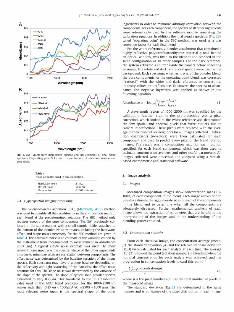
The Science-Based Calibration (SBC) (Marcbach, 2010) methodwas used to quantify all the constituents in the composition maps ineach blend at the predetermined rotations. The SBC method onlyrequires spectra of the pure components (Fig. 2A) previously col-lected in the same manner with a small sample holder attached tothe bottom of the blender. Noise estimates, including the hardware,offset, and slope noises necessary for the SBC method are given inTable 4. The hardware noise is an estimate of the variation caused bythe instrument from measurement to measurement in absorbanceunits (Au). A typical 2 mAu noise estimate was used. The mostrelevant noise input was the spectral shape of the other ingredientsin order to minimize arbitrary correlation between components. Theoffset noise was determined by the baseline variation of the imagespectra. Each spectrum may have a unique baseline depending onthe reflectivity and light scattering of the particles; the offset noiseaccounts for this. The slope noise was determined by the variance ofthe slope of the spectra. The slope of typical solid powder spectraestimated to vary 0.25 Au. This translated to the 0.1667 mAu/nmvalue used in the APAP blend prediction for the 1000–2500 nmregion such that 0:25 Au� 1000ðmA=AÞ� �

=ð2500 �1000 nmÞ. Themost relevant noise input is the spectral shape of the other

ingredients in order to minimize arbitrary correlation between thecomponents. For each component, the spectra of all other ingredientswere automatically used by the software module generating thecalibration equations. In addition, the final blend0s spectrum (Fig. 2B),called “operating point” in the SBC method, was used as a biascorrection factor for each final blend.

For the white reference, a blender attachment that contained ahighly reflective polytetrafluoroethylene material placed behindan optical window, was fixed to the blender and scanned in thesame configuration as all other samples. For the dark reference,the system activated a shutter inside the camera before collectingan image. The white and dark references0 spectra were used as thebackground. Each spectrum, whether it was of the powder blend,the pure components, or the operating point blend, was corrected(“ratioed”) with the white and dark references to convert theintensity values into reflectance. To convert the spectra to absor-bance, the negative logarithm was applied as shown in thefollowing equation.

Absorbance¼ � log 10Isample� IdarkIwhite� Idark

� �ð1Þ

A wavelength region of 1000–2500 nm was specified for thecalibration. Another step in the pre-processing was a pixelcorrection, which looked at the white reference and determinedthe few spatial and spectral pixels that were outliers due tocamera imperfections. These pixels were replaced with the aver-age of their non-outlier neighbors for all images collected. Calibra-tion coefficients (b-vectors) were then calculated for eachcomponent and used to predict every pixel of the blend rotationimages. The result was a composition map for each rotationspecified, for each blend component, which was then used toestimate concentration averages and other useful parameters. Allimages collected were processed and analyzed using a Matlab-based chemometric and statistical software.

3. Image analysis

3.1. Images

Measured composition images show concentration maps (0–100%) of each component in the blend. Each image allows one tovisually estimate the agglomerate sizes of each of the componentsin the blend and to determine when all the components areadequately dispersed. Further mathematical analysis of eachimage allows the extraction of parameters that are helpful in theinterpretation of the images and in the understanding of theblending process studied.

3.2. Concentration statistics

From each chemical image, the concentration average (mean,μ), the standard deviation (s) and the relative standard deviation(RSD) were calculated for each analyte at each turn. The average(Eq. (2)) showed the point (rotation number) in blending when thenominal concentration for each analyte was achieved, and theprogression in concentration levels toward this point.

μ¼∑P

p ¼ 1concentrationðpÞP

; ð2Þ

where p is the pixel number and P is the total number of pixels inthe measured image

The standard deviation (Eq. (3)) is determined in the samemanner and is a measure of the pixel distribution in each image,

Fig. 2. (A) Typical pure ingredients0 spectra and (B) examples of final blendspectrum (“operating point”) for each concentrations of each formulation andpure APAP.

Table 4Noise estimates used in SBC calibration.

Hardware noise 2 mAuOff-set noise 50 mAuSlope noise 0.1667 mAu/nm

J.G. Osorio et al. / Chemical Engineering Science 108 (2014) 244–257 247

indicating the composition range in which most of the pixels lie.

s¼

ffiffiffiffiffiffiffiffiffiffiffiffiffiffiffiffiffiffiffiffiffiffiffiffiffiffiffiffiffi∑P

p ¼ 1ðp�μÞ2P

sð3Þ

The relative standard deviation (RSD) is calculated from the ratioof the standard deviation (s) and the mean (μ) of each measuredimage. The RSD is a commonly used tool in the pharmaceuticalindustry to estimate the uniformity of a component within a blend.The customary RSD description of pharmaceutical blends is based onthe calculated variance of API concentration from one unit dose toanother. In the case of image analysis, the system was sensing thevariation of concentration from pixel to pixel, each covering anapproximate area of 30 mm�30 mm of the blend. Thus, the actualamount of material “sampled” is much smaller, and the RSDmeasured in these experiments is much higher, than the customaryunit dose sample RSD.

3.3. Fraction of pixels statistics

3.3.1. Within threshold“Within threshold” is the fraction of pixels that are within a

specified concentration threshold. The average concentration doesnot give an indication of whether there are many of pixels aboveor below this average. Calculating the fraction of pixels within athreshold may be useful, for example, if there is some criteria thatthe blend must be mixed to a point such that 95% of the blend iswithin 10% of the nominal composition. The criteria for acceptancedepend on the blend formulation requirements, and may bedifferent for each blend and component. The thresholds used forall components are shown in Table 5.

In order to calculate this quantity, a baseline value (the nominalcomposition) was selected in order to quantify the fraction of themeasured image that was within a certain range. A factor wasdefined to calculate the lower and upper limits of the threshold asspecified in Table 5. To determine the appropriate threshold levels,the images on a ternary scale were visualized. An example of animage in ternary scale is shown in Fig. 3. This shows the pixelswithin the threshold in gray, the pixels above the threshold inwhite, and the pixels below the threshold in black. This image

analysis allows the visual identification of the proper threshold.The image of a better mixed blend (later rotation) showed severalsmall aggregates (groups of white pixels), with most of the imagein gray and a few black areas. If the threshold was set too low, alarge fraction of the image was colored white. This was not arealistic size for aggregates and the threshold was increased. Forvery low concentration components, such as magnesium stearate,the threshold was set to the nominal (concentration716� thenominal concentration); for low to mid-range concentrationcomponents, a lower threshold factor is appropriate. For example,for the 10% APAP blend, the threshold was set to the nominal(concentration73� the nominal concentration). For higher con-centration components (10–40% w/w), 0.3� to 1.0� is an appro-priate threshold factor. The exact lower and upper thresholdsused in this study are given in Table 5. In some cases, the lowerthresholds are negative. Even though a negative concentrationdoes not have a physical meaning, the statistical distribution ofthe prediction values can have a wide range including negativepredicted concentrations.

3.3.2. Above thresholdThe fraction of pixels above a threshold indicate the presence of

agglomerates of pure components. This is important because thiscan determine whether a blend is homogeneous at the micro-scale. In order to estimate the fraction of the measured image thatdisplays aggregates, the pixels above the thresholds specified inTable 5 were determined. A threshold was specified as previouslyexplained. The uniformity of a blend is optimum if the fraction ofpixels above the threshold is close to zero. As an example, acriterion that the blend is complete is when less than 10% of theimage pixels are high points (above the threshold).

3.4. Aggregate size statistics (mean/median/maximumof aggregate sizes)

In order to determine the mean, median, or maximum aggre-gate size, the following algorithm was used. A pixel was part of anaggregate if it was above a certain specified threshold defined inthe same way as described above in Section 3.3.1. Aggregates weredefined as a group of x or more adjacent pixels all above thepredetermined concentration threshold, where the minimumaggregate size x is specified. The size of each aggregate and theirstatistics were calculated for each composition map for eachcomponent. The mean and maximum aggregate sizes were calcu-lated. Other aggregate size statistics can also be useful to char-acterize the progression of blending, such as the median aggregatesizes or skew and kurtosis. Mathematical descriptions of theseadditional statistical tools were omitted for sake of brevity.

Table 5Thresholds used for identification of aggregates, fraction “within threshold”, and“above threshold” statistics.

Blend Lower and upper thresholds (nominal7nominalnfactor)

Avicel (%) Lactose (%) APAP (%) MgSt (%)

1 30.9–64.1 26.1–68.9 �6.0–12.0 �22.5–25.52 28.6–59.4 24.2–63.8 0–20.0 �22.5–25.53 17.0–51.0 10.2–57.8 21.0–39.0 �22.5–25.5

Fig. 3. “Peaks and Valleys” display: gray areas are between the upper and lower thresholds (nominal concentration 7nominalnfactor), white areas are higher concentrationthan the upper threshold; black areas are concentrations less than the lower threshold.

J.G. Osorio et al. / Chemical Engineering Science 108 (2014) 244–257248

4. Results and discussion

4.1. Image results

Measured composition images from each ingredient were obtainedfor all conditions described in the experimental design. The visualinspection of the measured images helped to describe the mixingevolution of all the components. As examples, the composition imagesof 3%, 10% and 30% APAP blended at 25 RPM are shown in Fig. 4. Theseimages are on a color scale corresponding to a concentration gradientfrom 0% to 100%. The images show the mixing evolution of all thecomponents as a function of the number of revolutions. As evidencedby the images, for all blends, Avicel was added first, covering thewindow, and therefore the corresponding composition images startedat 100% and then approached the nominal concentration for Avicel.For 3% APAP (Fig. 4A), the nominal concentration of Avicel was

reached at around turn 45. Lactose was added second, not reachingthe window. Its concentration started at 0% and then approached itsnominal concentration between 20 and 30 turns. MgSt was added at40 revolutions, and therefore its concentration indicated 0% until then.After its addition, MgSt was detected as agglomerates but it was mixedefficiently after a few additional revolutions.

Visual inspection did not reveal substantial APAP agglomerates atthe 3% concentration level. It seemed that APAP was efficiently mixedafter a few revolutions. A few agglomerates of APAP were detectedeven after 40 rotations for higher concentrations. The agglomerateconcentration of SiO2 was higher in the first few rotations anddecreased as the blending process took place, as seen in the imagesfor all concentrations of APAP. Although the concentration of SiO2 islow and it was sieved before blending, it maintained agglomeratesthroughout the entire blending process. The detection of agglomer-ates indicates that the shear inside the mixer is not enough to

Fig. 4. Sample images: (A) 3% APAP, (B) 10% APAP and (C) 30% APAP. Other parameters: blender speed, 25 RPM.

J.G. Osorio et al. / Chemical Engineering Science 108 (2014) 244–257 249

Fig. 5. Comparison images for experiment 1 (A) Scientific Based Calibration (SBC) and (B) single wavelength at 1350 nm (color scale in absorbance units).

J.G. Osorio et al. / Chemical Engineering Science 108 (2014) 244–257250

completely break these agglomerates, which were already present orreformed in the SiO2 as a raw material before blending. The meanparticle size of the SiO2 used was �10 nm. Forces, such as van derWaals forces, between the SiO2 particles at this scale are large andeasily induce spontaneous agglomeration. Therefore, to improve theblending of SiO2, a shearing aid (intensifier bar) should be used insuch low-shear blender.

Similar blending behavior for Avicel, lactose and APAP wasdetected for experiments with 10% APAP and 30% APAP(Fig. 4B and C). In these examples, the two main components, Aviceland lactose, determined the blending end-point. Their micro-mixingevolution was seen in the composition images. The mixing of themain components took longer as the APAP concentration increased.The powder flow behavior changed with increasing APAP concentra-tion. Therefore APAP, as a cohesive material, governed the flow of theblend and other components as its concentration increased in theblends. It is known that as the concentration of a cohesive material isincreased in a powder blend, the flow properties of the powder blendworsen (i.e. the powder blend becomes more cohesive) (Osorio andMuzzio, 2013). The higher the concentration of APAP, the longer ittook for all the components – in particular Avicel – to become moredispersed (better mixed). One hypothesis for this phenomenon is thatthe similarity in particle size of Avicel and APAP, with APAP being amore cohesive material, might have a strong influence on the mixingrate of Avicel. In current practice, when a blend is monitored forhomogeneity, usually only the API homogeneity is taken into account(Wu et al., 2009). However, the homogeneity of other components isalso an important indication of when the blend is actually well mixed,and this is particularly important if the other ingredients performimportant functional roles. In the case described here, if only APAPwas being monitored, then a “homogeneous” blend would have beendetermined after a few rotations as shown in the images. The use ofthis in-line NIR-CI technique allows for the monitoring of all ingre-dients in a blend at once and is able to consider the effects of theimportant ingredients on the blending behavior.

The concentration maps as measured by the SBC method andabsorbance images at wavelength 1350 nm are shown in Fig. 5A and Bfor experiment 1, respectively. The SBC concentration images show thered spots where APAP agglomerates were detected by this calibrationmethod. The single wavelength (univariate) images at 1350 nm showthe spots where APAP has the most intensity in absorbance asindicated by the color bar. This serves as a brief comparison and“validation” showing that the SBC method actually detects APAPagglomerates and is able to measure the overall concentration ofAPAP as well as the other ingredients in each chemical image.

4.2. Concentration statistics

4.2.1. Average concentrationThe calculated average concentrations of the main components

as a function of the rotation number for the 25-RPM experimentsare shown in Fig. 6. The time it took for a blend to reach stablenominal composition increased with the increase in APAP con-centration, as observed in the images in Section 4.1. APAP reachednominal concentrations rather quickly, but the addition of MgStcaused a disturbance in the average concentration when detected.For these concentrations, APAP seemed to have reached itsnominal concentration value even before the addition of MgSt(Fig. 6A). After the addition of MgSt, APAP reached its nominalvalue around 50 revolutions into the blending process for all levelsof concentration. Avicel reached its nominal composition ataround 45 revolutions for 3% APAP, 80 revolutions for 10% APAP,and 180 revolutions for 30% APAP (Fig. 6B). Thus, it can be seenthat Avicel did indeed take longer to blend as the concentration ofAPAP was increased. Lactose reached its nominal composition ataround 20 revolutions for 3% APAP, and 40 revolutions for both10% and 30% APAP (Fig. 6C). Measurements were also obtained at15 and 35 RPM. The blender rotation rate did not significantlyaffect the blending profiles for any of the materials used (p � 0).It seems that at this level of shear rate, the rotation speed has

Fig. 6. Sample Average Concentrations for (A) APAP, (B) Avicel, and (C) lactose. For Avicel and lactose, the nominal concentration at 3% APAP was 47.5%, at 10% APAP was 44%,and at 30% APAP was 34%. Other parameters: blender speed at 25 RPM. Figures shown in different scales to point out differences in results.

J.G. Osorio et al. / Chemical Engineering Science 108 (2014) 244–257 251

negligible effect for these ingredients and concentrations (withcomparisons performed at the same number of rotations, whichroughly correspond to an equivalent amount of strain). For thisreason, only the curves for 25 RPM are shown here.

4.2.2. Relative standard deviationThe relative standard deviation (RSD) of each composition

image as a function of time was calculated for all the experimentsto study their blending profiles. A higher concentration of APAP(Fig. 7A) yielded a lower RSD. These results are common, and aredue to the natural tendency for this type of cohesive APAP to stayin aggregates, especially at low concentrations. The rotation ratedid not have a significant impact on the RSD for the blends used,but the number of revolutions did affect the RSD. This result is inagreement with previous results published by this group(Mehrotra and Muzzio, 2009). At the beginning of blending for3% APAP, small RSD differences were observed for the variousrotation rates. The difference in RSDs became less as the number ofrotations increased. In this case, the RSDs also seemed to continuedecreasing even at the final rotations. This means that APAP mightbecome even more evenly dispersed after 200 rotations; thereforemore rotations should be used. For 10% APAP, a decrease in RSDwas obtained up to 30 revolutions. The RSDs then reached aplateau. For 30% APAP, the lowest RSD was reached after a fewrevolutions with no clear trend. The rotation rate did not yield

significant differences in the RSD measurements for 10% and 30%APAP blends. The mixing curves for APAP were not well defined asit has been shown in previous work when measuring the bulkconcentration of this API (Mehrotra and Muzzio, 2009).

The Avicel RSD results did not to follow any particular trend(Fig. 7B). Nonetheless, the RSD results were higher for blends withhigher concentration of APAP – especially for 30% APAP. The RSDswere also slightly higher for 10% APAP when compared to 3% APAPblends. This is in agreement with the previous results shown herethat a higher concentration of APAP affected the manner in whichAvicel was blending. For lactose, on the other hand, the RSDdecreased with increasing number of revolutions (Fig. 7C). The RSDvalues were higher for the 30% APAP blends. The presence of higherAPAP concentration made it more difficult for Avicel and lactose toform a highly uniform blend. Lactose followed typical mixing curvesshowing both regimes usually encountered in powder mixing. Thefirst regime is driven by convection, wherein most of the bulk(macro) mixing occurs, and the second regime is driven by dispersionof particles, where most micro-mixing occurs. Lactose reached aminimum RSD with most of its mixing obtained by convection(Massol-Chaudeur et al., 2002). Further analysis of the RSD of 3%and 10% API cases at 25 RPM, as a function of image size (samplesize) was carried out to demonstrate their correlation (Fig. 8A). Themeasured RSD decreased as the sample size increased, as expected.The linearization using the natural log of the RSD2 and the image sizealso yielded the expected trend (Fig. 8B). This demonstrates that the

Fig. 7. Relative standard deviation (RSD) of (A) APAP, (B) Avicel and (C) lactose. 3%, 10%, and 30% represent the nominal concentration of APAP in the blends. Figures shown indifferent scales to point out differences in results.

J.G. Osorio et al. / Chemical Engineering Science 108 (2014) 244–257252

variability of an ingredient in a blend decreases with increasingsample size when measured using NIR-CI.

4.3. Fraction of pixels statistics

4.3.1. Within thresholdConcentration thresholds were chosen for each component

to calculate the fractions of pixels within the range as defined

previously. Thresholds chosen are listed in Table 5. The fraction ofpixels for APAP at different concentration levels are plotted inFig. 9A. For all concentration levels and rotation speeds, the fractionof pixels within the range reached at least 0.95. This means thatAPAP has mixed well within the range defined. There is no clearrelationship between this fraction and the concentration level ofAPAP. Overall, the fraction of pixels within range seemed to increaseas the number of rotations increased, especially during the first

Fig. 8. (A) RSD as a function of sample size (image size) and (B) linearization of RSD2 as a function of image size.

Fig. 9. Fraction of pixels within range of threshold for (A) APAP, (B) Avicel and (C) lactose.

J.G. Osorio et al. / Chemical Engineering Science 108 (2014) 244–257 253

rotations, reaching a maximum quickly. The fraction of pixels withinrange confirmed that APAP, in all cases studied here, mixed quickly.

The fraction of pixels within range for both Avicel (Fig. 9B) andlactose (Fig. 9C) increased with the number of revolutions until itreached a maximum value. Avicel reached its plateau after fewerrevolutions when the concentration of APAP was lower. Thisconfirms that there is a strong interaction between APAP andAvicel when blending. The fractions of pixels within range forAvicel were lower for higher concentrations of APAP in the blends.Lactose reached the fraction of pixels within range faster thanAvicel even for the blends with 30% APAP. The “good” flowproperties (indicated by larger particle size) of lactose promotefaster blending of this ingredient in all blends.

4.3.2. Above thresholdThe concentration thresholds chosen here were the upper

thresholds of those used in the “within threshold” calculations.For APAP (Fig. 10A), the fraction of pixels above the threshold wasvery low. The fraction of pixels above threshold increased duringthe first few revolutions, before adding MgSt. Once the MgSt wasadded (turn 40), the fraction of pixels reached a plateau, althoughthe variability from rotation to rotation was high in some cases.While the fraction of pixels above the threshold were low, themeasurements revealed larger possible aggregates even towardsthe end of the blending process. These results can describe thedispersive mixing of APAP in the blend. Although APAP seemed tohave been mixed well, the presence of agglomerates is still

evident. The fraction of pixels for Avicel (Fig. 10B) decreased withincreasing rotations and reached a minimum after 130 rotations.The Avicel results show the typical powder mixing kineticspreviously described. Avicel blending experienced fast mixing byconvection for the first 50 revolutions. In this phase, the fraction ofpixels above threshold was largely reduced. After 50 rotations,Avicel experienced mixing by dispersion. For lactose (Fig. 10C), thefraction of pixels above the threshold increased slightly the first 50rotations, but remained low all throughout blending. Since thefraction of pixels above the threshold were so low, substantialnoise was detected for lactose. There was no clear trend due to thevariation in concentration of lactose in the blends or to rotationrate. Disturbances after the addition of MgSt (turn 40) were alsodetected in the lactose measurements.

4.4. Aggregate size statistics

4.4.1. Mean aggregate sizeThe mean aggregate size was calculated using the same upper

thresholds as in Table 5. In addition, for a pixel to be considered partof an aggregate, it must be contiguous to a group of at least 9 (3�3)outlier pixels. In the experiments reported here, the mean aggregatesize for APAP (Fig. 11A) slightly decreased in the first few rotations.The APAP mean aggregate size reached a minimum quickly. Therewas not a clear correlation between APAP concentration and aggre-gate size in this case. These results are in accordance with all theprevious results shown. If the mean particle size diameter of APAP(45 mm) is used to calculate the mean area of APAP particles, then a

Fig. 10. Fraction of pixels above threshold for (A) APAP, (B) Avicel and (C) lactose.

J.G. Osorio et al. / Chemical Engineering Science 108 (2014) 244–257254

mean particle area of 1590 mm2 is obtained. Using this analogy, APAPis always in aggregates throughout the blending process. The meanaggregate size for Avicel (Fig. 11B) was high in the first few turns asAvicel was being mixed with the other components. The aggregatesize decreased substantially by turn 20. For the remainder of theblending process, the blends with a larger concentration of APAP(and less Avicel) had larger aggregates of Avicel. The mean aggregatesize of lactose (Fig. 11C) started high like that of Avicel, but sincelactose was the larger component and mixed faster, the mean lactoseaggregate size reached a minimum quickly.

4.4.2. Maximum aggregate sizeThe maximum aggregate size, indicating remaining unbroken

large aggregates, as a function of rotation rate for APAP and Avicel,is shown in Fig. 12. The detection of large aggregates is importantespecially when blending potent APIs. When large aggregates aredetected, the blending process must often be modified to improvethe mixing. In the case of APAP, there was no clear trend betweenAPAP concentration or blend rotation speed and maximum aggre-gate size (Fig. 12A). Large aggregates of APAP (15.5� larger thanthe mean particle area of APAP particles) were detected even atthe end of the blending process for 3% APAP blends. If this werethe case of a potent API, the blending process would have to bemodified to reduce such large aggregates.

For Avicel, the maximum aggregate size followed the sametrend as the mean aggregate size. The maximum size was largerfor lower concentrations of Avicel, and decreased quickly with

more revolutions (Fig. 12B). In some experiments, the first fewrotations showed large aggregates of lactose, but after a coupleturns of the blender there was not a clear trend in maximumaggregate size (Fig. 12C). It is interesting to note that the two mainingredients, lactose and Avicel, act quite differently in the blend.The large Avicel aggregates continue to be broken down graduallyas blending progresses, but large lactose aggregates remain, evenat later turns, as evidenced by the outliers in the plot. Having largeaggregates of high concentration excipients is not as critical,although these should also be well mixed to ensure the rightdispersion of the API and other components. For SiO2, the max-imum aggregate size did not show any correlation with APAPconcentration or rotation speed, but in a few experiments, largeaggregates remained even at later turns. For such low concentra-tion ingredients, imaging was able to capture the statistically smalloccurrence of remaining relatively large aggregates. For MgSt,aggregates were only detected immediately after its addition. Thisconcludes that MgSt was mixed quickly after a few rotations ofblending and aggregates could no longer be detected.

5. Conclusions

A new in situ near-infrared chemical imaging technique(imMixTM) designed to characterize micro-mixing in pharmaceu-tical powder blends was introduced in this article. This techniqueused non-contact monitoring of the blending process, eliminatingthe bias introduced when using typical extractive sampling

Fig. 11. Mean aggregate size for (A) APAP, (B) Avicel, and (C) lactose.

J.G. Osorio et al. / Chemical Engineering Science 108 (2014) 244–257 255

techniques. The spectral data was analyzed using the Science-Based Calibration (SBC) method to obtain concentration images ofthe ingredients in nine different blends in this experimentalmodel. Each image allowed the estimation of the size of agglom-erates and was used as a visual tool to help determine a suitablemixing time when all the components have formed a well-mixedblend. The mean concentration and RSD as a function of blendingtime was obtained from all images to further characterize theblending process. The time required for a blend to reach thenominal composition increased with the increase in APAP con-centration. This was mainly due to the interaction of APAP andAvicel. It was concluded that the rotation rate, using the 1-l bin-blender did not have an impact on the RSD, but the number ofrevolutions affected the blend homogeneity (RSD) of the maincomponents.

Statistical analysis of each image was used to obtain detailedinformation about the blending progression of each of the com-ponents in the blends. The number of pixels above a predeter-mined concentration threshold and the fraction of pixels within aspecified range of the nominal composition were used to char-acterize the blending progression. The fraction of pixels within thethreshold was independent of APAP concentration. The fraction ofpixels both within the threshold and above the threshold indicatedthat Avicel blended at a significantly slower rate than lactose.Avicel blended in fewer revolutions when the concentration ofAPAP was lower. The mean aggregate size statistics also supportedthe finding that Avicel blended at a slower rate than lactose. Themaximum aggregate size analysis of the near-infrared chemical

images provided a sensitive tool to detect aggregates of low-doseactive materials that could pose a hazard if they remainedunblended. Large APAP aggregates were detected in some blendseven at later rotations. This was an indication that APAP was stillpresent in the blend in form of agglomerates.

The imMix system showed to be useful in characterizing thedistribution of aggregate sizes of the model API and excipients usedfor this study. The hyperspectral imaging-based blend monitoringcan help in the development of pharmaceutical powder blendformulations. Further studies have been performed using variousAPIs with different particle size distributions, shapes and cohesionproperties to understand these effects, and will be summarized in alater publication.

Acknowledgment

We thank Professor Rodolfo Romañach for providing his helpand valued input during the final writing stage of this manuscript.

References

Beer, T.D., Burggraeve, A., Fonteyne, M., Saerens, L., Remonb, J.P., Vervaet, C., 2011.Near infrared and Raman spectroscopy for the in-process monitoring ofpharmaceutical production processes. Int. J. Pharm. 417, 32–47.

Brone, D., Muzzio, F.J., 2000. Enhanced mixing in double-cone blenders. PowderTechnol. 110, 179–189.

Fig. 12. Maximum aggregate size for (A) APAP, (B) Avicel and (C) lactose.

J.G. Osorio et al. / Chemical Engineering Science 108 (2014) 244–257256

Daumann, B., Fath, A., Anlauf, H., Nirschl, H., 2009. Determination of the mixingtime in a discontinuous powder mixer by using image analysis. Chem. Eng. Sci.64, 2320–2331.

El-Hagrasy, A.S., Morris, H.R., D0Amico, F., Lodder, R.A., Drennen , J.K., 2001. Near-infrared spectroscopy and imaging for the monitoring of powder blendhomogeneity. J. Pharm. Sci. 90, 1298–1307.

Hardy, E.H., Hoferer, J., Kasper, G., 2007. The mixing state of fine powders measuredby magnetic resonance imaging. Powder Technol. 177, 12–22.

Hyvärinen, T., Herrala, E., Jussila, J., 2011. High Speed Hyperspectral ChemicalImaging, Oulu, Finland. Specim (http://www.specim.fi)ohttp://www.middletonresearch.com/pdfs/HighSpeedHyperspectralChemicalImagingite.pdf4(accessed 3.9.2012).

Krämer, K., Ebel, S., 2000. Application of NIR reflectance spectroscopy for theidentification of pharmaceutical excipients. Anal. Chim. Acta 420, 155–161.

Li, W., Woldu, A., Kelly, R., McCool, J., Bruce, R., Rasmussen, H., Cunningham, J., Winstead,D., 2007. Measurement of drug agglomerates in powder blending simulationsamples by near infrared chemical imaging. Int. J. Pharm. 350, 369–3873.

Llusa, M., Levin, M., Snee, R.D., Muzzio, F.J., 2010. Measuring the hydrophobicity oflubricated blends of pharmaceutical excipients. Powder Technol. 198, 101–107.

Lyon, R.C., Lester, D.S., Lewis, E.N., Lee, E, Yu, L.X., Jefferson, E.H., Hussain, A.S., 2002.Near-infrared spectral imaging for quality assurance of pharmaceutical pro-ducts: analysis of tablets to assess powder blend homogeneity. AAPS Pharm.Sci. Technol. 3, 1–15.

Ma, H., Anderson, C.A., 2008. Characterization of pharmaceutical powder blends byNIR chemical imaging. J. Pharm. Sci. 97, 3305–3320.

Marcbach, R., 2010. Multivariate Kalibrierung, Selektivität und die SBC-Methode.Chemie Ingenieur Technik 82, 453–466.

Massol-Chaudeur, S., Berthiaux, H., Dodds, J.A., 2002. Experimental study of themixing kinetics of binary pharmaceutical powder mixtures in a laboratory hoopmixer. Chem. Eng. Sci. 57, 4053–4065.

Mehrotra, A., Muzzio, F.J., 2009. Comparing mixing performance of uniaxial andbiaxial bin blenders. Powder Technol. 196, 1–7.

Muzzio, F.J., Goodridge, C.L., Alexander, A., Arratia, P., Yang, H., Sudah, O., Mergen, G.,2003. Sampling and characterization of pharmaceutical powders and granularblends. Int. J. Pharm. 250, 51–64.

Muzzio, F.J., Llusa, M., Goodridgea, C.L., Duonga, N.H., Shen, E., 2008. Evaluating themixing performance of a ribbon blender. Powder Technol. 186, 247–254.

Muzzio, F.J., Robinson, P., Wightman, C., Brone, D., 1997. Sampling practices inpowder blending. Int. J. Pharm. 155, 153–178.

Muzzio, F.J., Shinbrot, T., Glasser, B.J., 2002. Powder technology in the pharmaceu-tical industry: the need to catch up fast. Powder Technol. 124, 1–7.

Osorio, J.G., Muzzio, F.J., 2013. Effects of powder flow properties on capsule fillingweight uniformity. Drug Dev. Ind. Pharm. 39, 1464–1475.

Perrault, M., Bertrand, F., Chaouki, J., 2010. An investigation of magnesium stearatemixing in a V-blender through gamma-ray detection. Powder Technol. 200,234–245.

Pingali, K., Mendez, R., Lewis, D., Michniak-Kohnb, B., Cuitino, A., Muzzio, F., 2011.Mixing order of glidant and lubricant – influence on powder and tabletproperties. Int. J. Pharm. 409, 269–277.

Pingali, K.C., Shinbrot, T., Hammond, S.V., Muzzio, F.J., 2009. An observed correla-tion between flow and electrical properties of pharmaceutical blends. PowderTechnol. 192, 157–165.

Porfire, A., Rus, L., Vonica, A.L., Tomuta, I., 2012. High-throughput NIR-chemometricmethods for determination of drug content and pharmaceutical properties ofindapamide powder blends for tabletting. J. Pharm. Biomed. Anal. 70, 301–309.

Portillo, P.M., Muzzio, F.J., Ierapetritou, M.G., 2006. Characterizing powder mixingprocesses utilizing compartment models. Int. J. Pharm., 320

Ravn, C., Skibsted, E., Bro, R., 2008. Near-infrared chemical imaging (NIR-CI) onpharmaceutical solid dosage forms—comparing common calibration approaches.J. Pharm. Biomed. Anal. 48, 554–561.

Realpe, A., Velazquez, C., 2003. Image processing and analysis for determination ofconcentrations of powder mixtures. Powder Technol. 134, 193–200.

Reich, G., 2005. Near-infrared spectroscopy and imaging: basic principles andpharmaceutical applications. Adv. Drug Del. Rev. 57, 1109–1143.

Rozo, J.I.J., Zarow, A., Zhou, B., Pinal, R., Iqbal, Z., Romanach, R.J., 2011. Comple-mentary near-infrared and Raman chemical imaging of pharmaceutical thinfilms. J. Pharm. Sci. 100, 4888–4895.

Sabin, G.P., Breitkreitz, M.C., Souza, A.M.d., Fonseca, P.d., Calefe, L., Moffa, M.,Poppi, R.J., 2011. Analysis of pharmaceutical pellets: an approach using near-infrared chemical imaging. Anal. Chim. Acta 706, 113–119.

Šaŝić, S., Kong, A., Kaul, G., 2013. Determining API domain sizes in pharmaceuticaltablets and blends upon varying milling conditions by near-infrared chemicalimaging. Anal. Methods 5, 2360–2368.

Sommier, N., Porion, P., Evesque, P., Leclerc, B., Tchoreloff, P., Couarraze, G., 2001.Magnetic resonance imaging investigation of the mixing-segregation process ina pharmaceutical blender. Int. J. Pharm. 222, 243–258.

Susana, L., Canu, P., Santomaso, A.C., 2011. Development and characterization of anew thief sampling device for cohesive powders. Int. J. Pharm. 416, 260–267.

Vasilenko, A., Glasser, B.J., Muzzio, F.J., 2011. Shear and flow behavior of pharma-ceutical blends – method comparison study. Powder Technol. 208, 628–636.

Venables, H.J., Wells, J.I., 2002. Powder Sampling. Drug Dev. Ind. Pharm. 28,107–117.

Wu, H., Tawakkul, M., White, M., Khan, M.A., 2009. Quality-by-Design (QbD): anintegrated multivariate approach for the component quantification in powderblends. Int. J. Pharm. 372, 39–48.

J.G. Osorio et al. / Chemical Engineering Science 108 (2014) 244–257 257