Characterization of complex fluids using small angles scattering techniques

O. Diat

OutlineBrief and classical introduction to scatteringmethods

•Form and Structure factors•Examples for contrast variation or dilution •Example with an oriented mesoporous AlO3 structure(K. Lagrené thesis)

references

Detector

Incident beam(planar wave)

rdreeR

ERdE rqiRkiS

srrr rrrr

)(1

4

1)( .).(

0 ρπ

−−=

0

dV

r

ρ(r)

θ

R

Fundamental equation of the instantaneous scattering amplitude

Hyp: far field detection, weak scattering

ii brr )()(rr

∑= ρρ ρρρ −=∆

∫−− ∆=

V

rqiRkiS rdere

RERE i

rrr rrrr.).(

0 )(1

4

1)( ρ

π

=−=2

sin4

q and θ

λπ

is kkqrrr

rdreeR

ERdE rqiRkiS

srrr rrrr

)(1

4

1)( .).(

0 ρπ

−−=

0

dV

r

ρ(r,t)

θ

R

fundamental equation of the instantaneous scattering amplitude

∫−− ∆=

V

rqiRkiS rdere

RERE i

rrr rrrr.).(

0 )(1

4

1)( ρ

π

For an assembly of discreteparticles

[ ] rdrrRrrdr j

N

jjj

rrrr)()()(

1

ρδρ ∆+−=∆ ∑=

j

j

j Rqi

qG

jrqi

j

Vj

N

jS erderqE

rrrr

444 3444 21

rrr .

)(

).(

1

])([)( ρ∆∝ ∫∑=

drjrj

Rj+1Rj

Scattering intensity Is(qq)

∑∑−−==

j k

RRqikjS

kjeqGqGEEqI).(** )()(.)(

rrrrrr

j

j

j Rqi

qG

jrqi

j

Vj

N

jS erderqE

rrrr

444 3444 21

rrr .

)(

).(

1

])([)( ρ∆∝ ∫∑=

part

partSkj

js

VG

qasG

qGqP

qPVG

qGG

V

NqGNqGqI

.)0( and

0 1)0(

)()(factor Form

)(...)0(

)()0()()()(

2

2

22

2222

ρ

ρ

∆=

→→=

∆Φ====∑=

r

rrrr

For diluted system (uncorrelated scatterers and identical)

cmcm

eb

eT

122

0

10.28.04

−==πε 3cm/cmin Th

molecularrayX b

V

Z=−ρ

FEDORS table, polymer engineering, 14 (2), 1974, 147-154

A density of scattering length

Left: Nuclear scattering length for thermal neutrons, b in 10−13 cm, versus the MA (in dotted line the variation for X-rays, linear in Z)Right: coherent and incoherent neutron scattering cross-sections(en barns=10-28 m2) for some elements and isotopes. Large area of the circle means large the cross-section.

The scattering intensity is the FT of pair-correlation function p(R)

dRqR

qRRR

RdeR

RqI

RrdRrrR

Rqi

S

V j

)sin()(~4

nsorientatio allaver averagean with

)(~)(~ of ansformFourier tr)( and

)()()()(~

functionon distributidistancepair p(R)

22

0

.2

2

2

43421

rr

rr

rrrrvr

rr

=

∞

−

∆∝

∆

∆∝

=−∆∆=∆

∫

∫

∫

ρπ

ρ

ρ

γρρρ

j

k

Rik=50

R50 100

p(R)

∑∑−−==

j k

RRqikjS

kjeqGqGEEqI).(** )()(.)(

rrrrrr

R50 100

p(R)

ρ(R)

Pair distributionexperiment

FT

Collimation effectRadiation smearingStatistical errorQmax/Qmin

Real space vs reciprocal space

Form factor

•Pedersen, J.S. (1997), Adv. Colloid Interface Sci., 70, 171 •SASfit

…. And so on

Structure factorFor concentred system (identical scatterers) and centrosymmetric

[ ] ∞→→−=−

∆Φ=+=

∫∞

qasdRqR

qRRRg

V

NqS

qSqPVqIV

NqG

V

NqI

S

partSS

s

0sin

1)(41)(factor structure

)()(...)()()(

2

0

2'2

π

ρr

If g(R) is the probability of finding the centre of any particle at a distance R from the centre of a given particle then for N particles in a volume V , (N/V )g(R)dV is the numberof particles in volume element dV at a distance R from a given particle.

TF

For concentred system (identical scatterers) and centrosymmetric

[ ] ∞→→−+=

∆Φ=+=

∫∞

qasdRqR

qRRRg

V

NqS

qSqPVqIV

NqG

V

NqI

S

partSS

s

1sin

1)(41)(factor structure

)()(...)()()(

2

0

2'2

π

ρr

Structure factor

Structure factorSeveral approximation:Ex: Monodisperse approximation: the interaction potential between particles are spherical symmetric and independent of the particle size that allows to reallydecompose in product of FF and SF

The calculation of S(q) is further complicated in the case of polydisperse systems …..

Pontoni, JCP 03

Stiky hard sphere ex.

Form factor

•What to do when the system is concentrated, when size and distance between scattering entities are similar ?

Pb can be solved using multiple parameters but what the physicsbehind?

•Play with contrast variation (SAXS and SANS)

•Play with dilution (if possible) – ex information insertion

•Porod and invariant analysis

Why to play with contrast variation

contrast

J. Gummel, thesis 06

θθθθ

3SO H− +− +− +− + 3SO TMA− +− +− +− +

N++++3CH

3CH

3CH

3CH

Protonated counterion TMA+

Another example of concentrated system:Fuel cell membrane – Nafion, a perfluo-sulfonated polymer (ionomer)

16 %45 %

80 %

65 %

85 %

ΦΦΦΦp

Hydration

continuous structure swelling

100 %

85 %

15 %

Dry membrane

Swollenmembrane

Hyper-swollenmembrane

Scattering evolution as a function of water swellingSAXS or SANS

• q-1 regime

elongated object

q-1

cylinder diameter d = 44Å (±±±± 20%)Shell thickness e = 5Å

polymer DLD ρρρρp = 4.9 x1010 cm/cm3

PTFE Amorphous 4.21x1010 cm/cm3

PTFE Crystalline 5.08x1010 cm/cm3

2I(q) F (q)∝∝∝∝Neglect the structure factor

Form factor of aggregateslow polymer volume fraction (ΦP = 16 %)

Rod-like aggregates in hyper-swollen membrane

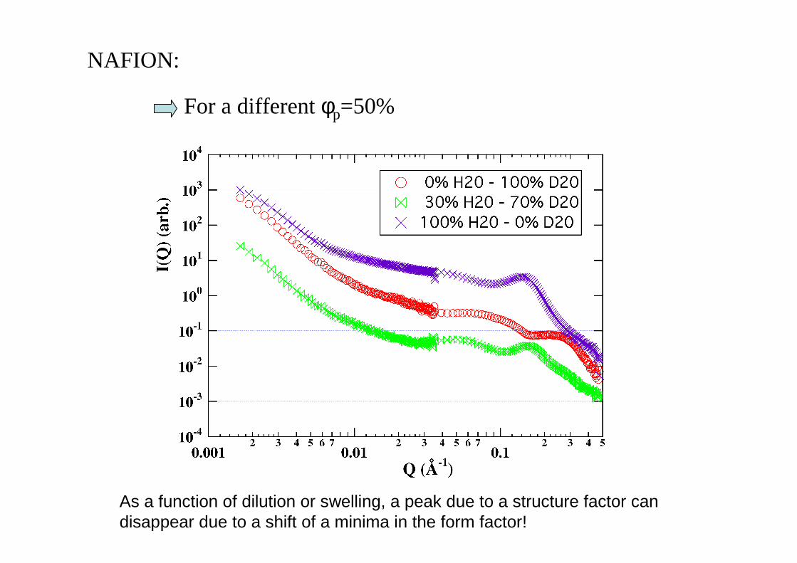
NAFION:

For a different φp=50%

As a function of dilution or swelling, a peak due to a structure factor candisappear due to a shift of a minima in the form factor!

Similar shape of the division curves.

No change of the scatteringaggregates

Ok for assumption of oriented objects

2I(q) S(q).F (q)∝∝∝∝Oriented rod-like

aggregates

Experimental divisionsimulation

0,01

0,1

1

10

0,01 0,1

q (-1)

Naf-16%

Naf-35%

Naf-50%

Naf-85%

Cylinder organisationLarger polymer volume fraction from 35 to 80 %

NAFION: Schematic model

Gierke (82) model

RGD model(Rubatat 04)

NAFION: Schematic model

RGD model(Rubatat 04)

10

100

1000

0,01 0,1 1

φp (%)

-1/2

Swelling law

•Importance of contrast variation (SAXS / SANS) usingsame structural parameters, to eliminate the SF contribution as a first step, to discriminate betweencouples of structural parameters

•Importance of the dilution or swelling law as φ-1, φ-1/2, φ-1/3

•Check if the shape of the individual particles is similarwhatever the dilution or concentrationIf not, reorientation, new molecular assembling, second or first order transition ..

Things to keep in mind when performing SAS experiments

Analyzing the scattering curves over a large range of q to obtain the best set of structural parameters (size, aggregation number, interaction distance)

It allows to understand the thermodynamic of the system

Limiting form of I(q)

For non-interacting particles and for qR<<1, thenGuinier Law

In case of homogeneous particles with a sharpinterface, it exist an asymptotic limit, qR>>1 thatleads to the Porod law:

And finally, the invariant (for an incompressible and two-phase system)

)3

)(exp(...)(

22 G

parts

qRVqI −∆Φ= ρr

42 .)(2)( −Σ∆= qqI ρπ

222 )1(2)( ρπ ∆Φ−Φ== ∫ dqqIqQ

To perform scattering experiments

•To use always refererence sample and empty cellin similar conditions

•To known the sample thickness and otherscattering parameters

• To get data in absolute units

• to the largest (suitable) q-range as possible (whennecessary)

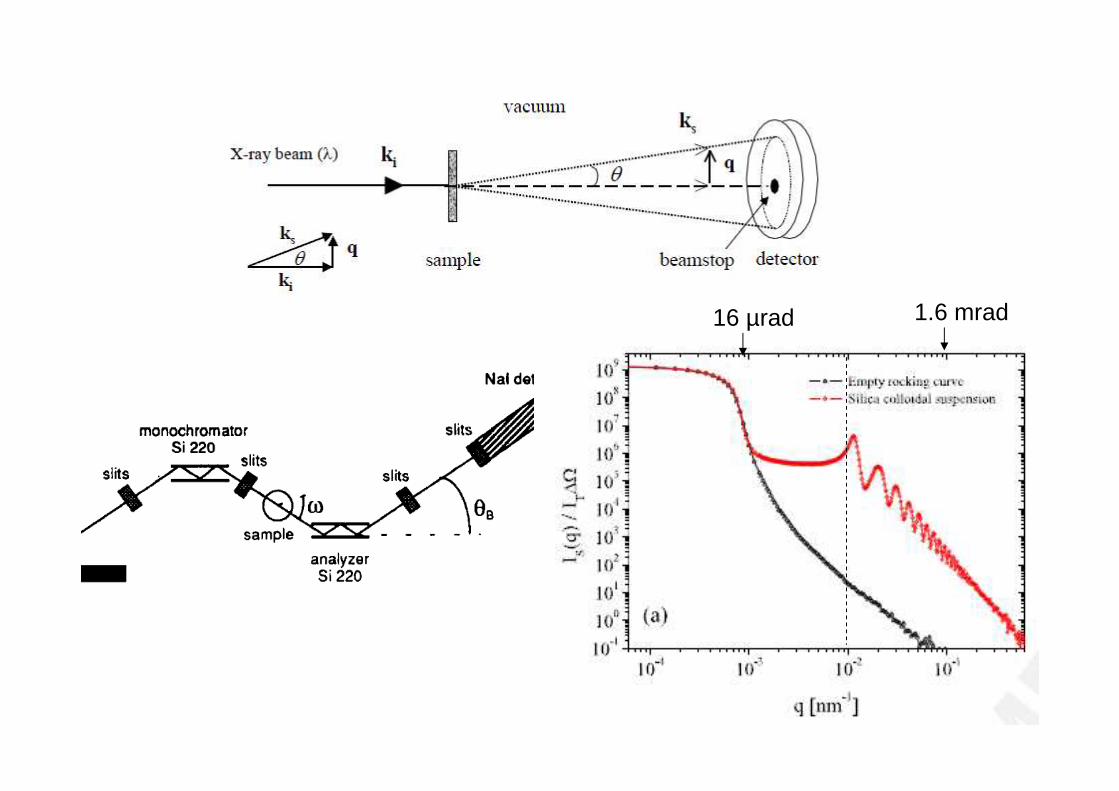
1.6 mrad16 µrad

Common SAXS experiment

∆ΩΩ

= ...),(1

.).().()( etd

d

VTI acq

λθσλελψθ

Flux: nbr photons /s

Differential scattering cross section(cm-1/ solid angle)

Detector efficiency

Sample thickness (homo)

)exp( eT µ−=

optimum of exp(-µe) for e=1/µ or a transmission T=1/e=0.37

, µ: linear attenuation coefficiant

transmission

Acquisition timephotons in direction θ

Flux and efficiency has to be determined using calibrant (lupolen, water or other solvent..)

sacqabs etT

I

d

d

VI

...).(

),(1 exp

∆Ω=

Ω=

λψλθσ

22

0

2 )).(1(2. ρϕϕπ ∆−== ∫∞

ssabs dqqIQ

( )2

4

)(2

lim

ρπ ∆

=Σ ∞→qabsqIPorod law

Invariant

• To extract S/V:Porod law using the absolute intensity and a

contraste estimated using a contraste variation method (S/V=25m2/cm3)

From SEM (S/V=28m2/cm3)

Contrast variation (K. Lagrené data)

cohAcoh

matrix

ODHOHHHsolvent

bM

dN

v

b ==

−+=

ρ

ρϕρϕϕρ22

).1(.)(

Thank you and see the attachedreferences for more details

• 1. Guinier, A. and Fournet, G. (1955) Small-Angle Scattering of X-rays, Wiley, New York.

• 2. Glatter, O. and Kratky, O., Eds., (1982), Small-Angle X-ray Scattering, Academic Press, London.

• 3. Feigin, L.A. and Svergun, D.I. (1987) Structure Analysis by Small-Angle X-ray and Neutron Scattering, Plenum Press, New York.

• 4. Brumberger, H., Ed., (1995) Modern Aspects of Small-Angle Scattering, Kluwer Academic, Dordrecht.

• 5. Lindner, P. and Zemb, T., Eds., (2002) Neutrons, X-rays and Light : Scattering methods applied to soft condensed matter, Elsevier, Amsterdam.

• 6. Schmidt, P.W. (1995) in Modern Aspects of Small-Angle Scattering, Brumberger, H., Ed., p. 1, Kluwer Academic, Dordrecht.

• X-ray data booklet LBL, California• Neutron Data Booklet, ILL/ITU• SASfit software package, PS Institure