Characterization of coarse particulate matter in the ... · Characterization of coarse particulate...

Atmos. Chem. Phys., 13, 1311–1327, 2013www.atmos-chem-phys.net/13/1311/2013/doi:10.5194/acp-13-1311-2013© Author(s) 2013. CC Attribution 3.0 License.

EGU Journal Logos (RGB)

Advances in Geosciences

Open A

ccess

Natural Hazards and Earth System

Sciences

Open A

ccess

Annales Geophysicae

Open A

ccessNonlinear Processes

in Geophysics

Open A

ccess

Atmospheric Chemistry

and PhysicsO

pen Access

Atmospheric Chemistry

and Physics

Open A

ccess

Discussions

Atmospheric Measurement

Techniques

Open A

ccess

Atmospheric Measurement

Techniques

Open A

ccess

Discussions

Biogeosciences

Open A

ccess

Open A

ccess

BiogeosciencesDiscussions

Climate of the Past

Open A

ccess

Open A

ccess

Climate of the Past

Discussions

Earth System Dynamics

Open A

ccess

Open A

ccess

Earth System Dynamics

Discussions

GeoscientificInstrumentation

Methods andData Systems

Open A

ccess

GeoscientificInstrumentation

Methods andData Systems

Open A

ccess

Discussions

GeoscientificModel Development

Open A

ccess

Open A

ccess

GeoscientificModel Development

Discussions

Hydrology and Earth System

Sciences

Open A

ccess

Hydrology and Earth System

Sciences

Open A

ccess

Discussions

Ocean Science

Open A

ccess

Open A

ccess

Ocean ScienceDiscussions

Solid Earth

Open A

ccess

Open A

ccess

Solid EarthDiscussions

The Cryosphere

Open A

ccess

Open A

ccess

The CryosphereDiscussions

Natural Hazards and Earth System

Sciences

Open A

ccess

Discussions

Characterization of coarse particulate matter in the western UnitedStates: a comparison between observation and modeling

R. Li 1,2, C. Wiedinmyer1, K. R. Baker3, and M. P. Hannigan2

1National Center for Atmospheric Research, 1850 Table Mesa Drive, Boulder, CO, USA2Department of Mechanical Engineering, University of Colorado, Boulder, CO, USA3Office of Air Quality, Planning, and Standards (OAQPS), United States Environmental Protection Agency,Research Triangle Park, NC, USA

Correspondence to:R. Li ([email protected])

Received: 13 January 2012 – Published in Atmos. Chem. Phys. Discuss.: 3 May 2012Revised: 2 October 2012 – Accepted: 16 January 2013 – Published: 1 February 2013

Abstract. We provide a regional characterization of coarseparticulate matter (PM10−2.5) spanning the western UnitedStates based on the analysis of measurements from 50 sitesreported in the US EPA Air Quality System (AQS) andtwo state agencies. We found that the observed PM10−2.5concentrations show significant spatial variability and dis-tinct spatial patterns, associated with the distributions of landuse/land cover and soil moisture. The highest concentrationswere observed in the southwestern US, where sparse vege-tation, shrublands or barren lands dominate with lower soilmoistures, whereas the lowest concentrations were observedin areas dominated by grasslands, forest, or croplands withhigher surface soil moistures. The observed PM10−2.5 con-centrations also show variable seasonal, weekly, and diur-nal patterns, indicating a variety of sources and their relativeimportance at different locations. The observed results werecompared to modeled PM10−2.5 concentrations from an an-nual simulation using the Community Multiscale Air Qualitymodeling system (CMAQ) that has been designed for regu-latory or policy assessments of a variety of pollutants includ-ing PM10, which consists of PM10−2.5 and fine particulatematter (PM2.5). The model under-predicts PM10−2.5 obser-vations at 49 of 50 sites, among which 14 sites have annualobservation means that are at least five times greater thanmodel means. Model results also fail to reproduce their spa-tial patterns. Important sources (e.g. pollen, bacteria, fungalspores, and geogenic dust) were not included in the emis-sion inventory used and/or the applied emissions were greatlyunder-estimated. Unlike the observed patterns that are morecomplex, modeled PM10−2.5 concentrations show the simi-

lar seasonal, weekly, and diurnal pattern; the temporal allo-cations in the modeling system need improvement. CMAQdoes not include organic materials in PM10−2.5; however,speciation measurements show that organics constitute a sig-nificant component. The results improve our understandingof sources and behavior of PM10−2.5 and suggest avenues forfuture improvements to models that simulate PM10−2.5 emis-sions, transport and fate.

1 Introduction

Concentrations of atmospheric particulate matter (PM) arecurrently regulated by the US Environmental ProtectionAgency (EPA) with National Ambient Air Quality Standards(NAAQS) for both PM2.5 (fine particles; particulate mat-ter with a diameter less than 2.5 µm) and PM10 (particu-late matter with a diameter less than 10 µm) (http://www.epa.gov/air/criteria.html). In the United States, there is anannual average standard and a 24-h average standard forPM2.5. The 3-yr average of the annual mean PM2.5 con-centrations must not exceed 15.0 µg m−3, and the 3-yr av-erage of the 98th percentile of 24-h concentrations at eachpopulation-oriented monitor within an area must not exceed35 µg m−3. The 24-h average PM10 concentration standard of150 µg m−3 must not be exceeded more than once per year onaverage over 3 yr. The European Community also regulatesatmospheric particulate matter with legal limit values (e.g.daily limit value of 50 µg m−3 for PM10) under Directive2008/50/EC of the European Parliament and of the Council

Published by Copernicus Publications on behalf of the European Geosciences Union.

http://www.epa.gov/air/criteria.html

http://www.epa.gov/air/criteria.html

1312 R. Li et al.: Characterization of coarse particulate matter in the western United States

of 21 May 2008 on ambient air quality and cleaner air for Eu-rope (http://ec.europa.eu/environment/air/quality/legislation/existing leg.htm).

Airborne PM10 consists of both fine particles (PM2.5) andcoarse particles (PM10−2.5; particulate matter with a diam-eter between 2.5 and 10 µm). Therefore, to meet the PM10standards, not only PM2.5 but PM10−2.5 concentrations needto be controlled. Moreover, recent epidemiological and tox-icological studies show that PM10−2.5 concentrations havebeen linked to mortality (e.g. Malig and Ostro, 2009; Perezet al., 2008; Zanobetti and Schwartz, 2009) as well as res-piratory and cardiovascular morbidity (Branis et al., 2010;Brunekreef and Forsberg, 2005; Host et al., 2008; Sandstromand Forsberg, 2008; Zhang et al., 2002).

In addition to health impacts and legal regulations, atmo-spheric particles can considerably affect climate directly byinfluencing incoming and outgoing radiation, and indirectlyby serving as cloud condensation nuclei (CCN) and ice nu-clei (IN), influencing the formation and lifetimes of cloudsand precipitation as well as atmospheric chemistry (DeMottet al., 2003; Koehler et al., 2009; Krueger et al., 2004; Ku-mar et al., 2009, 2011; Solomon et al., 2007; Wang et al.,2007; Wurzler et al., 2000). Aerosols can also affect biogeo-chemical cycles, which can alter carbon fluxes and furtherinteract with climate, by influencing physical environment(e.g. diffuse radiation, precipitation and temperature) and bydepositing nutrients (e.g. nitrogen, phosphorous, and iron) ortoxins (e.g. copper) to ecosystems (Mahowald, 2011; Pay-tan et al., 2009). The indirect effects of aerosols on climateare very uncertain (Mahowald, 2011; Solomon et al., 2007).PM10−2.5 components (e.g. sea salt and soil dust) contributeconsiderably to global aerosol mass, optical thickness, andsurface particle concentrations (Birmili et al., 2008; Textor etal., 2006). Therefore, to better quantify the effects of atmo-spheric particles, the characteristics of not only fine particlesbut coarse particles need to be understood.

While PM2.5 is primarily emitted from combustion pro-cesses or formed in the atmosphere through chemical re-actions and gas-to-particle conversion processes, PM10−2.5predominantly originates from abrasive mechanical pro-cesses, with sources such as geogenic dust, sea salt, dustfrom construction activities, tire wear, brake wear, and or-ganic bioaerosols such as bacteria, pollen and fungal spores(Edgerton et al., 2009; Harrison et al., 2001; Kelly et al.,2010; Malm et al., 2007; Sesartic and Dallafior, 2011; Zhuet al., 2009). Controlling variables on these sources includeland use, land cover, and environmental conditions (e.g. tem-perature, soil moisture, snow/ice cover, wind speed). Someof these sources are a result of natural processes (e.g. wind-blown dust in a desert), while others are more closely tied tohuman activities (e.g. construction). Additionally, PM10−2.5has a higher deposition velocity, i.e., shorter atmospheric res-idence time, than PM2.5. These combined facts mean thatPM10−2.5 will have different spatial and temporal variabil-ity than PM2.5. Recent studies investigated the characteristics

of PM10−2.5 in a few US cities including Los Angeles, CA(Pakbin et al., 2010), Detroit, MI (Thornburg et al., 2009),Rochester, NY (Lagudu et al., 2011), and Denver and Gree-ley, CO (Clements et al., 2012). However, little research hasinvestigated the spatial and temporal variability of PM10−2.5concentrations at a regional scale, or the relationships be-tween concentrations and land use/land cover and soil mois-ture dependent on geographical location.

Accurate PM10−2.5 modeling tools are needed by boththe scientific community and regulatory agencies for miti-gation strategy development and health effect assessments.PM10−2.5 is simulated as part of the US EPA’s Commu-nity Multiscale Air Quality (CMAQ) modeling system (Byunand Schere, 2006). However, the model performance forPM10−2.5 has not been explicitly assessed because over thepast decade both PM model and measurement studies haveprimarily focused on PM2.5. CMAQ and other chemicaltransport models have been primarily assessed for their per-formance for PM2.5 or PM10 (Baldasano et al., 2011; Chuanget al., 2011; Foley et al., 2010; Konovalov et al., 2011; Lonatiet al., 2010; Sokhi et al., 2008; Wang et al., 2008). Yet, sincefine and coarse particles have different sources as well asdifferent chemical composition and potential health effects,they should be considered as separate classes of pollutants assuggested by Wilson and Suh (1997) and assessed individu-ally.

Given the importance of coarse particles for air quality, cli-mate, and human health risk assessments, improvements toour knowledge of the sources and characteristics of PM10−2.5are essential. In this paper, we investigate the temporal andspatial patterns of measured PM10−2.5 concentrations in thewestern United States. The results of this analysis provide in-sights to the sources and fate of PM10−2.5 and motivate moreaccurate models that describe PM10−2.5 emissions, transport,and atmospheric concentrations.

2 Methods

This study was carried out using both observations and modelsimulations for an entire year (2005) over a domain that cov-ers the western United States (see Fig. 1).

2.1 Measurement data

While abundant ambient PM2.5 and PM10 mass concentra-tion data are available, direct measurements of PM10−2.5mass concentrations are very limited. Therefore, our studyobtained co-located measurements of PM10 and PM2.5. Weobtained all available observed hourly-averaged PM10 andPM2.5 concentration data in the western United States (seeFigs. 1 and 2) for 2005 from the Air Quality System(AQS) datamart (http://www.epa.gov/ttn/airs/aqsdatamart/)and from two state agencies. From the AQS, we obtainedhourly co-located PM10 and PM2.5 concentration data for

Atmos. Chem. Phys., 13, 1311–1327, 2013 www.atmos-chem-phys.net/13/1311/2013/

http://ec.europa.eu/environment/air/quality/legislation/existing_leg.htm

http://ec.europa.eu/environment/air/quality/legislation/existing_leg.htm

http://www.epa.gov/ttn/airs/aqsdatamart/

R. Li et al.: Characterization of coarse particulate matter in the western United States 1313

39

Fig. 1. Map of monitoring locations and land use / land cover in the study domain (sites 786

having hourly data are represented with black plus symbols, and black circles represent 787

sites having daily data). 788

789

Fig. 1. Map of monitoring locations and land use/land cover in the study domain (sites having hourly data are represented with black plussymbols, and black circles represent sites having daily data).

40

Fig. 2. Measured annual mean PM10-2.5 concentrations at measurement sites in the 790

western United States. 791

792

793 Fig. 2. Measured annual mean PM10−2.5 concentrations at mea-surement sites in the western United States.

23 sites. Co-located hourly measurements from two addi-tional sites were obtained from state agencies: Santa Bar-bara, CA (AQS Site Number: 060830011) from the Cal-ifornia Air Resources Board (http://www.arb.ca.gov/aqd/

aqdcd/aqdcddld.htm), and Denver, CO (AQS Site Number:080310002) from Colorado Department of Public Health andEnvironment (B. L. Rink, personal communication, 2011).These 25 sites are shown as plus symbols in Fig. 1 (also de-scribed in Table 1). To fill spatial gaps of hourly data, weobtained daily measurements (24-h filter samples) from theAQS for an additional 25 sites in the domain, shown as cir-cles in Fig. 1 (also described in Table 1). The 24-h measure-ments were taken every three days at two sites (Riverside site,CA, AQS Site Number of 060830011 and Salt Lake City,Utah, AQS Site Number of 490353006), and every 6 daysat the other sites. Details of all measurement sites, includingassociated environmental conditions output from the Penn-sylvania State University/National Center for AtmosphericResearch Mesoscale Meteorology Model (MM5) (i.e. hourlyaverage temperature, wind speed, and surface soil moisture),are presented in Table 1. The concentrations of PM10−2.5were calculated as the difference between co-located PM10and PM2.5 concentrations at all hourly and daily sites.

2.2 Model simulations

To obtain insights for regional PM10−2.5 modeling, modelsimulations were carried out for the western United States.The Community Multiscale Air Quality (CMAQ) modeling

www.atmos-chem-phys.net/13/1311/2013/ Atmos. Chem. Phys., 13, 1311–1327, 2013

http://www.arb.ca.gov/aqd/aqdcd/aqdcddld.htm

http://www.arb.ca.gov/aqd/aqdcd/aqdcddld.htm


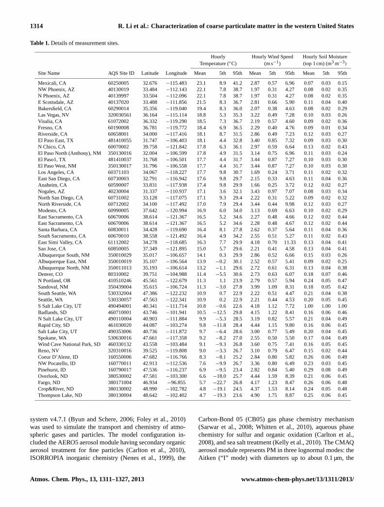
Table 1.Details of measurement sites.

Hourly Hourly Wind Speed Hourly Soil MoistureTemperature (◦C) (m s−1) (top 1 cm) (m3 m−3)

Site Name AQS Site ID Latitude Longitude Mean 5th 95th Mean 5th 95th Mean 5th 95th

Mexicali, CA 60250005 32.676 −115.483 23.1 8.9 41.2 2.87 0.57 6.96 0.07 0.03 0.15NW Phoenix, AZ 40130019 33.484 −112.143 22.1 7.8 38.7 1.97 0.31 4.27 0.08 0.02 0.35N Phoenix, AZ 40139997 33.504 −112.096 22.1 7.8 38.7 1.97 0.31 4.27 0.08 0.02 0.35E Scottsdale, AZ 40137020 33.488 −111.856 21.5 8.3 36.7 2.81 0.66 5.90 0.11 0.04 0.40Bakersfield, CA 60290014 35.356 −119.040 19.4 8.3 36.0 2.07 0.38 4.63 0.08 0.02 0.29Las Vegas, NV 320030561 36.164 −115.114 18.8 5.3 35.3 3.22 0.49 7.28 0.10 0.03 0.26Visalia, CA 61072002 36.332 −119.290 18.5 7.3 36.7 2.19 0.57 4.60 0.09 0.02 0.36Fresno, CA 60190008 36.781 −119.772 18.4 6.9 36.5 2.29 0.40 4.76 0.09 0.01 0.34Riverside, CA 60658001 34.000 −117.416 18.1 8.7 31.5 2.86 0.49 7.23 0.12 0.03 0.27El Paso East, TX 481410055 31.747 −106.403 18.1 4.4 32.8 3.40 0.85 7.32 0.09 0.03 0.30N Chico, CA 60070002 39.758 −121.842 17.8 6.3 36.1 2.97 0.59 6.64 0.13 0.02 0.43El Paso North (Anthony), NM 350130016 32.004 −106.599 17.8 4.9 31.5 3.14 0.75 6.96 0.11 0.03 0.24El Paso1, TX 481410037 31.768 −106.501 17.7 4.4 31.7 3.44 0.87 7.27 0.10 0.03 0.30El Paso West, NM 350130017 31.796 −106.558 17.7 4.4 31.7 3.44 0.87 7.27 0.10 0.03 0.30Los Angeles, CA 60371103 34.067 −118.227 17.7 9.8 30.7 1.69 0.24 3.71 0.11 0.02 0.32East San Diego, CA 60730003 32.791−116.942 17.6 9.8 29.7 2.15 0.33 4.63 0.11 0.04 0.36Anaheim, CA 60590007 33.831 −117.938 17.4 9.8 29.9 1.66 0.25 3.72 0.12 0.02 0.27Nogales, AZ 40230004 31.337 −110.937 17.1 3.6 32.1 3.43 0.97 7.07 0.08 0.03 0.34North San Diego, CA 60731002 33.128 −117.075 17.1 9.3 29.4 2.22 0.31 5.22 0.09 0.02 0.32North Riverside, CA 60712002 34.100 −117.492 17.0 7.9 29.4 3.44 0.44 9.98 0.12 0.03 0.27Modesto, CA 60990005 37.642 −120.994 16.9 6.0 34.0 3.13 0.69 6.63 0.10 0.02 0.29East Sacramento, CA 60670006 38.614−121.367 16.5 5.2 34.6 2.27 0.48 4.66 0.12 0.02 0.44East Sacramento, CA 60670006 38.614−121.367 16.5 5.2 34.6 2.28 0.48 4.67 0.12 0.02 0.44Santa Barbara, CA 60830011 34.428−119.690 16.4 8.1 27.8 2.62 0.37 5.64 0.11 0.04 0.36South Sacramento, CA 60670010 38.558−121.492 16.4 4.9 34.2 2.55 0.51 5.27 0.11 0.02 0.43East Simi Valley, CA 61112002 34.278 −118.685 16.3 7.7 29.9 4.18 0.70 11.33 0.13 0.04 0.41San Jose, CA 60850005 37.349 −121.895 15.0 5.7 29.6 2.21 0.41 4.58 0.13 0.04 0.41Albuquerque South, NM 350010029 35.017−106.657 14.1 0.3 29.9 2.86 0.52 6.66 0.15 0.03 0.26Albuquerque East, NM 350010019 35.107−106.564 13.9 −0.2 30.1 2.52 0.57 5.41 0.09 0.02 0.25Albuquerque North, NM 350011013 35.193 −106.614 13.2 −1.1 29.6 2.72 0.61 6.31 0.13 0.04 0.38Denver, CO 80310002 39.751 −104.988 11.4 −5.5 30.6 2.73 0.63 6.07 0.18 0.07 0.46N Portland, OR 410510246 45.561 −122.679 11.3 1.1 23.9 2.79 0.57 5.94 0.24 0.05 0.47Sandoval, NM 350439004 35.615 −106.724 11.3 −3.0 27.8 3.99 1.09 8.31 0.18 0.05 0.42South Seattle, WA 530332004 47.386 −122.232 10.9 0.7 22.9 2.22 0.51 4.47 0.21 0.04 0.38Seattle, WA 530330057 47.563 −122.341 10.9 0.2 22.9 2.21 0.44 4.53 0.20 0.05 0.45S Salt Lake City, UT 490494001 40.341 −111.714 10.8 −0.6 22.6 4.18 1.12 7.72 1.00 1.00 1.00Badlands, SD 460710001 43.746 −101.941 10.5 −12.5 29.8 4.15 1.22 8.41 0.16 0.06 0.46N Salt Lake City, UT 490110004 40.903 −111.884 9.9 −5.3 28.5 3.19 0.82 5.57 0.21 0.04 0.49Rapid City, SD 461030020 44.087 −103.274 9.8 −11.8 28.4 4.44 1.15 9.80 0.16 0.06 0.45Salt Lake City, UT 490353006 40.736 −111.872 9.7 −6.4 28.6 3.00 0.77 5.49 0.20 0.04 0.45Spokane, WA 530630016 47.661 −117.358 9.2 −8.2 27.0 2.55 0.50 5.50 0.17 0.04 0.49Wind Cave National Park, SD 460330132 43.558−103.484 9.1 −9.3 26.8 3.60 0.75 7.41 0.16 0.05 0.45Reno, NV 320310016 39.525 −119.808 9.0 −3.3 26.7 3.10 0.79 6.47 0.15 0.02 0.44Coeur D’Alene, ID 160550006 47.682 −116.766 8.3 −8.1 25.2 2.84 0.80 5.82 0.26 0.06 0.49NW Pocatello, ID 160770011 42.913 −112.536 7.6 −9.9 26.7 3.36 0.80 6.49 0.23 0.03 0.45Pinehurst, ID 160790017 47.536 −116.237 6.9 −9.5 23.4 2.82 0.84 5.40 0.29 0.08 0.49Overlook, ND 380530002 47.581 −103.300 6.6 −18.0 25.7 4.44 1.59 8.39 0.21 0.06 0.45Fargo, ND 380171004 46.934 −96.855 5.7 −22.7 26.8 4.17 1.23 8.47 0.26 0.06 0.48Crop&River, ND 380130002 48.990 −102.782 4.8 −19.1 24.5 4.37 1.53 8.14 0.24 0.05 0.48Thompson Lake, ND 380130004 48.642 −102.402 4.7 −19.3 23.6 4.90 1.75 8.87 0.25 0.06 0.45

system v4.7.1 (Byun and Schere, 2006; Foley et al., 2010)was used to simulate the transport and chemistry of atmo-spheric gases and particles. The model configuration in-cluded the AERO5 aerosol module having secondary organicaerosol treatment for fine particles (Carlton et al., 2010),ISORROPIA inorganic chemistry (Nenes et al., 1999), the

Carbon-Bond 05 (CB05) gas phase chemistry mechanism(Sarwar et al., 2008; Whitten et al., 2010), aqueous phasechemistry for sulfur and organic oxidation (Carlton et al.,2008), and sea salt treatment (Kelly et al., 2010). The CMAQaerosol module represents PM in three lognormal modes: theAitken (“I” mode) with diameters up to about 0.1 µm, the



Table 2.Summary of statistical analyses of measured and modeled PM10−2.5 concentrations.

Site Name Number of Measured PM10−2.5 Modeled PM10−2.5 Ratio of Measured toSamples (µg m−3) (µg m−3) Modeled PM10−2.5

Mean 5th 95th CV Mean 5th 95th CV Mean 95th CV

South Seattle, WA 8675 9.0 0.0 25.3 1.0 1.9 0.4 4.2 0.7 4.8 6.1 1.5El Paso1, TX 8664 25.2 1.3 80.6 1.5 7.8 1.3 24.0 1.0 3.2 3.4 1.6El Paso North (Anthony), NM 8642 34.8 4.4 96.2 1.5 18.4 3.0 49.0 0.8 1.9 2.0 1.8Seattle, WA 8622 14.8 0.3 38.0 1.0 2.2 0.5 4.7 0.6 6.8 8.0 1.6Fargo, ND 8606 12.1 2.6 34.6 1.0 6.1 0.9 16.8 0.9 2.0 2.1 1.2Thompson Lake, ND 8605 6.7 1.7 17.7 1.0 1.8 0.3 4.9 0.9 3.6 3.6 1.1Crop&River, ND 8508 8.1 1.2 22.0 1.0 3.3 0.4 8.9 0.9 2.4 2.5 1.1Coeur D’Alene, ID 8478 8.6 0.0 26.0 1.5 5.3 1.1 14.0 0.8 1.6 1.9 1.8Albuquerque East, NM 8471 10.0 0.0 27.7 1.2 8.1 1.5 20.1 0.8 1.2 1.4 1.6El Paso West, NM 8455 34.8 2.4 118.8 1.9 7.8 1.3 24.0 1.0 4.5 5.0 2.0Albuquerque South, NM 8447 21.8 0.0 68.8 1.6 11.9 1.9 30.1 0.8 1.8 2.3 2.0Wind Cave National Park, SD 8432 2.8 0.0 8.9 1.4 0.6 0.1 1.6 0.9 4.7 5.5 1.6Albuquerque North, NM 8375 17.7 0.0 57.3 1.4 10.8 1.8 26.3 0.7 1.6 2.2 1.9Spokane, WA 8286 15.9 0.0 52.6 1.6 4.1 0.6 11.0 0.9 3.9 4.8 1.9Rapid City, SD 8268 28.4 0.4 109.5 1.5 4.4 0.9 12.5 0.9 6.5 8.8 1.7Badlands, SD 8259 4.9 0.0 14.5 1.5 0.8 0.1 2.1 0.8 6.4 7.0 1.8Sandoval, NM 8099 31.4 0.0 118.4 1.5 4.7 0.8 12.7 0.8 6.7 9.3 1.8Denver, CO 8036 12.0 0.0 33.1 1.0 6.2 1.2 16.8 0.8 1.9 2.0 1.2Overlook, ND 7996 6.1 1.0 15.5 0.9 1.0 0.2 2.6 0.9 6.3 5.9 1.0NW Pocatello, ID 7928 14.3 0.0 51.7 2.0 3.6 0.7 11.1 1.1 4.0 4.7 1.9Santa Barbara, CA 7533 17.5 2.0 37.0 0.7 4.6 0.7 12.5 0.8 3.8 3.0 0.8El Paso East, TX 7390 28.4 1.8 85.0 1.8 4.9 0.7 14.8 1.0 5.8 5.7 1.9Pinehurst, ID 7162 8.5 0.0 26.5 1.6 1.2 0.2 3.4 0.9 6.9 7.9 1.8East Sacramento, CA 6384 11.4 0.0 26.7 0.8 4.7 1.1 11.9 0.8 2.4 2.2 1.1Nogales, AZ 6135 49.4 3.5 181.9 1.5 1.8 0.4 3.9 0.6 27.7 47.0 2.4Riverside, CA 120 31.0 4.6 59.5 N/A 8.1 2.8 13.4 N/A 3.8 4.4 N/ASalt Lake City, UT 111 11.1 1.4 25.4 N/A 4.2 1.5 10.5 N/A 2.6 2.4 N/AS Salt Lake City, UT 61 12.7 0.0 28.6 N/A 3.5 1.0 6.4 N/A 3.6 4.5 N/ALos Angeles, CA 61 9.8 0.0 18.6 N/A 7.9 2.9 12.5 N/A 1.2 1.5 N/AAnaheim, CA 60 11.4 1.6 21.9 N/A 9.5 4.4 15.7 N/A 1.2 1.4 N/AEast Sacramento, CA 59 8.2 0.0 21.6 N/A 4.7 1.9 9.1 N/A 1.7 2.4 N/ANorth Riverside, CA 58 25.6 4.7 51.0 N/A 5.0 1.1 9.3 N/A 5.1 5.5 N/AFresno, CA 57 14.5 1.8 35.7 N/A 2.6 0.9 5.3 N/A 5.6 6.7 N/ASan Jose, CA 57 9.2 0.0 17.2 N/A 9.5 4.3 17.8 N/A 1.0 1.0 N/AN Portland, OR 57 6.7 0.0 13.4 N/A 4.8 1.8 11.0 N/A 1.4 1.2 N/AReno, NV 56 14.5 3.6 26.3 N/A 5.1 1.7 10.3 N/A 2.8 2.6 N/ANW Phoenix, AZ 55 30.4 5.8 60.6 N/A 10.0 4.9 16.3 N/A 3.0 3.7 N/AN Phoenix, AZ 55 19.4 1.9 38.8 N/A 10.0 4.9 16.3 N/A 1.9 2.4 N/ALas Vegas, NV 53 20.8 2.1 37.5 N/A 12.1 5.0 25.2 N/A 1.7 1.5 N/AEast San Diego, CA 53 14.7 5.8 24.0 N/A 7.9 2.1 13.3 N/A 1.9 1.8 N/AN Salt Lake City, UT 50 12.8 0.5 33.0 N/A 5.2 1.9 12.5 N/A 2.4 2.6 N/AMexicali, CA 49 34.7 13.0 66.8 N/A 6.0 2.7 10.4 N/A 5.8 6.4 N/AModesto, CA 49 13.1 0.3 33.9 N/A 4.4 1.7 8.2 N/A 3.0 4.1 N/AEast Simi Valley, CA 48 11.7 1.8 24.1 N/A 2.6 0.7 5.4 N/A 4.5 4.5 N/AN Chico, CA 47 11.3 1.4 24.1 N/A 1.7 0.7 3.2 N/A 6.6 7.6 N/ASouth Sacramento, CA 47 8.8 0.0 23.0 N/A 5.2 1.8 12.4 N/A 1.7 1.9 N/AE Scottsdale, AZ 46 39.9 9.6 74.0 N/A 8.7 3.9 14.6 N/A 4.6 5.1 N/ABakersfield, CA 46 23.4 3.7 49.9 N/A 3.9 2.2 6.3 N/A 6.0 7.9 N/ANorth San Diego, CA 45 11.2 2.1 20.7 N/A 6.6 1.1 10.9 N/A 1.7 1.9 N/AVisalia, CA 43 21.0 1.4 49.0 N/A 2.4 1.1 4.4 N/A 8.8 11.1 N/A



accumulation (“J” mode) with diameters between 0.1 and2.5 µm, and coarse particles (“K” mode) having diametersbetween 2.5 and 10 µm. Model estimates of speciated PM inthe coarse mode are summed for comparison to the obser-vation data. CMAQ was run for a domain that covers thewestern United States with a resolution of 12 km (Figs. 1and 6). A larger domain with 36 km square grid cells cov-ering the continental United States, southern Canada, andnorthern Mexico was used to supply hourly boundary con-ditions to the 12 km square grid cell domain. Horizontallyand vertically varying initial conditions for the 36 km do-main were extracted from a 2005 global simulation of theGEOS-CHEM model, which also provided spatially varyingboundary conditions to the 36 km CMAQ model simulationon a 3-hourly basis.

Gridded meteorological data for CMAQ and SMOKE (theSparse Matrix Operator Kernel Emissions modeling system)(Houyoux et al., 2000) were generated using MM5 version3.7.4 (http://www.mmm.ucar.edu/mm5) with the Pleim-Xiuboundary layer and land surface model (Pleim and Xiu, 2003;Xiu and Pleim, 2001), Kain-Fritsh 2 cumulus parameteriza-tion (Kain, 2004), RRTM longwave (Mlawer et al., 1997),Dudhia shortwave (Dudhia, 1989), and Reisner 2 mixedphase moisture schemes (Reisner et al., 1998). Three dimen-sional analysis nudging was applied only above the boundarylayer for moisture and temperature and over the entire verti-cal atmosphere for winds. The MM5 simulations resolve thevertical atmosphere up to 100 mb with 34 layers, which werereduced to 14 layers by MCIP (Meteorology-Chemistry In-terface Processor) (Otte and Pleim, 2010) for emissions andphotochemical models with the thinnest layers near the sur-face to best resolve the diurnal boundary layer cycles. Theheight of the first model layer is approximately 38 m.

Simulations were performed for the year 2005 with 3 daysof spin-up at the end of 2004 that were not included in theanalysis. Anthropogenic emissions used to drive the model-ing system were based on the 2005 National Emission Inven-tory (NEI) (http://www.epa.gov/ttnchie1/net/2005inventory.html). Biogenic emissions were estimated with the BEISmodel using hourly temperature and solar radiation as in-put (Pierce et al., 1998). Emissions were processed to hourlygridded input to CMAQ with the SMOKE model version 2.5(Houyoux et al., 2000). Over the modeling domain, annualPM10−2.5 emissions were dominated by the non-point areasector (86 %), and their primary sources include fugitive dustfrom paved roads, unpaved roads, road construction, residen-tial construction, non-residential construction, and agricul-tural tilling. The inventory did not include emission estimatesof wind-blown (geogenic) dust. Sea salt emissions were sim-ulated online within CMAQ following Kelly et al. (2010).

3 Measurement analyses

3.1 Spatial variability

Table 2 presents a summary of statistical analyses of mea-sured and modeled PM10−2.5 concentration data at all siteshaving either hourly or daily data, including mean, 5th per-centile, 95th percentile and coefficient of variation (CV). CVis defined as the following:

CV =Standard deviation of time series

Mean of time series(1)

The measured PM10−2.5 concentrations have a distinct spa-tial pattern in the western United States as seen in Fig. 2,which shows observed annual mean PM10−2.5 concentra-tions at all measurement sites. The highest concentrationswere observed at sites in the southwestern US, where shrub-lands and barren/sparse vegetation dominate (Fig. 1) withgenerally lower surface soil moistures and higher temper-atures (Table 1). The lowest concentrations were found atsites dominated by grasslands, forest, or croplands with gen-erally higher surface soil moistures and lower temperatures(Fig. 1; Table 1). Given the dominance of shrublands andbarren/sparse vegetation along with very dry soils in thesouthwestern US, the higher concentrations in this regionare likely caused by fugitive dust emissions, which includegeogenic dust. Table 2 shows that all sites having annualmean concentrations that are higher than 17.7 µg m−3 arelocated to the south of∼ 36◦ N, except for the Rapid Citysite, which has high winds (Table 1) and is significantly in-fluenced by fugitive dust from several industrial facilities(primarily limestone quarrying and processing and cementmanufacturing and processing facilities) (http://denr.sd.gov/documents/neap.pdf).

Measured PM10−2.5 concentrations show strong spatialvariations across the western US; the annual mean of mea-sured PM10−2.5 concentrations is more than 17 times higherat the Nogales site in Arizona than at the Wind CaveNational Park site in South Dakota. Even sites in closeproximity showed significant variability. For example, al-though the N. Phoenix (040139997) and the N. W. Phoenix(040130019) sites are located very close to each other(∼ 5 km), the annual mean of measured concentrations dif-fered substantially, from 19.4 to 30.4 µg m−3, respectively.In Albuquerque, NM, the annual mean measured concen-tration is more than two times higher at the AlbuquerqueSouth site (21.8 µg m−3) than at the Albuquerque East site(10.0 µg m−3), although they are located within the samecity (∼ 13 km apart). The differences in PM10−2.5 concen-trations between the sites can be even greater at finer tempo-ral resolutions. The daily average concentration on 8 April2005 (during a PM10−2.5 episode) was 3.75 times higher atthe Albuquerque South site (130 µg m−3) than at the Albu-querque East site (34.7 µg m−3); the maximum hourly con-centration on this day was about 6 times higher at the former


http://www.mmm.ucar.edu/mm5

http://www.epa.gov/ttnchie1/net/2005inventory.html

http://www.epa.gov/ttnchie1/net/2005inventory.html

http://denr.sd.gov/documents/neap.pdf

http://denr.sd.gov/documents/neap.pdf


site (571 µg m−3) than at the latter site (95.4 µg m−3). Ob-served annual average PM10−2.5 concentrations at the RapidCity site (28.4 µg m−3) were more than 10 times higher thanthose at the Wind Cave National Park site (2.8 µg m−3), eventhough these two sites are only 61 km apart.

The spatial variability of measured PM10−2.5 at both ur-ban and regional scales was assessed with the correlationcoefficients for measured hourly concentrations, calculatedbetween all sites having hourly measurements. Moderate tostrong correlations were observed between some sites lo-cated in close proximity to one another, including the foursites in El Paso, TX (r2

= 0.24–0.58), two sites in Albu-querque, NM (r2

= 0.28), three sites in the northeastern partof the domain (Crop&River, Thompson Lake, and Overlookin North Dakota;r2

= 0.21–0.36), three sites in the north-west (Spokane, Pinehurst, and Coeur D’Alene;r2

= 0.23–0.37) and two sites in Seattle (r2

= 0.2). The p-values forthese correlations are all less than 0.0001, so they were con-sidered significant. No correlation was observed between anyother combinations of the site pairs. Very little correlationwas seen even over relatively small distances between somesites, such as two sites in New Mexico (Sandoval and Al-buquerque East;r2

= 0.05) and three sites in South Dakota(Rapid City, Badlands, and Wind Cave National Park;r2

=

0.00–0.03), suggesting that these sites are impacted by dif-ferent sources or have a different proximity to sources. Thesepoor correlations along with high spatial variability also sug-gest that PM10−2.5 concentrations are often influenced by lo-cal factors.

3.2 Temporal patterns

3.2.1 Variability

Figure 3 presents the time series of measured daily aver-age PM10−2.5 concentrations (red lines or squares) at se-lected representative sites having hourly (Fig. 3a–c) or 24-h(Fig. 3d–f) measurements. The green lines in Fig. 3 repre-sent simulated daily average concentrations from the mod-eling study, which will be discussed subsequently. Figure 3demonstrates that measured daily average PM10−2.5 concen-trations have strong temporal variations at each site withepisodic high levels. The CV of measured PM10−2.5 concen-trations is not less than 1.0 at 22 of 25 sites, ranging from 0.7to 2.0 (see Table 2). Figure 3a shows that measured PM10−2.5concentrations exceeded the level of the PM10 NAAQS (24-h average of 150 µg m−3) for many days in 2005 in El Paso.This result highlights the necessity to understand the behav-ior of coarse particles in order to develop mitigation strate-gies to keep the PM10 concentrations at safe levels.

3.2.2 Seasonal patterns

Figure 3 also reveals seasonal patterns. The measuredPM10−2.5 concentrations show different seasonal patterns de-

pendent on location. At some sites (e.g. Fargo and Fresno,two inland or valley sites influenced by agricultural sources,shown in Fig. 3c and f), the measured concentrations show aseasonal pattern with lower values in winter months. At thosesites in the southwestern US and on the west coast (e.g. ElPaso West, Seattle, and Riverside shown in Fig. 3a–b, d), themeasured PM10−2.5 concentrations seem to be more uniformover the year, with some episodic increased concentrations.

3.2.3 Weekly patterns

The red lines in Fig. 4 show one-year average weekly pat-terns of measured PM10−2.5 concentrations at selected hourlysites. There are primarily three different average weekly pat-terns of observed PM10−2.5 concentrations at the hourly sites.The first pattern shows that the measured PM10−2.5 concen-trations are∼ 50 % lower for weekends than for weekdays(e.g. the Seattle site shown in Fig. 4a), reflecting significantinfluences of weekday versus weekend human activities onPM10−2.5 concentrations at these sites. The second weeklypattern, on the contrary, shows that there is little differencein the observed concentrations between weekdays and week-ends (e.g. the El Paso West site shown in Fig. 4c). The week-day versus weekend human activities have a negligible im-pact on observed PM10−2.5 concentrations at these sites. Thethird pattern, which lies in between the previous two pat-terns, suggests that human activities have a moderate influ-ence on the observed PM10−2.5 concentrations, with one-yearaverage levels being about 20 % lower during weekends thanweekdays (e.g. the Santa Barbara site in Fig. 4b). The pat-terns are apparently dependent on the relative importance ofthe weekday versus weekend human activities on PM10−2.5concentrations compared to other sources.

3.2.4 Diurnal patterns

The red lines in Fig. 5a–d show one-year average diurnal pat-terns of measured PM10−2.5 concentrations at selected hourlysites. The measured concentrations exhibit different diurnalpatterns varying with location. Observed PM10−2.5 concen-trations at some sites (e.g. see Fig. 5a for the Denver site)show a typical diurnal pattern associated with on-road traf-fic. There is a rush-hour peak in the morning, followed by adecrease corresponding to a reduced volume of traffic and anincreased mixing layer height in the middle of the day. Thenthere is a late afternoon rush-hour peak and another reductionafterwards. However, the measured patterns at other sites aremore complicated with some having significantly bigger af-ternoon peaks (e.g. Fig. 5b for El Paso West) but with othershaving significantly bigger morning peaks (e.g. Fig. 5c forSeattle). The diurnal pattern at the Rapid City site, whichis significantly influenced by industrial facilities (Sect. 3.1),is completely different: the concentrations at night are rel-atively small (15 µg m−3), and increase steadily, reaching amaximum value of about 42 µg m−3 in the middle of the



41

Fig. 3. Measured (red lines or symbols) and modeled (green lines) daily-average PM10-2.5 794

concentrations at representative hourly (a-c) and 24-hour (d-f) sites. Note that the 24-hour 795

measurements were taken every 3 days at the Riverside site (d) but every 6 days at the 796

San Jose (e) and Fresno (f) sites. Note the differences in scale. 797

798 (a) El Paso West (b) Seattle 799

800 (c) Fargo (d) Riverside 801

802 Julian day 803

(e) San Jose (f) Fresno 804

Fig. 3.Measured (red lines or symbols) and modeled (green lines) daily-average PM10−2.5 concentrations at representative hourly(a–c)and24-h (d–f) sites. Note that the 24-h measurements were taken every 3 days at the Riverside site(d) but every 6 days at the San Jose(e) andFresno(f) sites. Note the differences in scale.

day, then decrease gradually to 19 µg m−3 in the evening.These different patterns reflect a range of different contribut-ing sources at different locations.

4 Comparison of observations with model simulations

4.1 Model performance for the magnitude of PM10−2.5concentrations

In addition to the measured concentrations, Table 2 alsoshows statistical analyses of CMAQ-predicted PM10−2.5concentrations. Table 2 reveals that the CMAQ model un-derestimated annual PM10−2.5 concentrations at all sites ex-cept for San Jose, CA, where the agreement between mod-eled and measured annual average concentrations is the bestamong all sites. However, the good agreement at the SanJose site is only for the annual mean concentration; the

model failed to reproduce the seasonal pattern at this site(see Sect. 4.3.2). The mean ratio of measured to modeledannual PM10−2.5 concentrations, averaged across all sites, ismore than 4, with the maximum ratio of 27 at the Nogalessite in the southern Arizona. While CMAQ generally under-estimated PM10−2.5 concentrations at almost all sites, thereare variations in model performance at different locations.While the modeled and measured annual mean concentra-tions agree within a factor of two at 16 sites, 20 sites havemeasured annual mean concentrations that are more than fourtimes higher than modeled values (Table 2). Among these 20sites, 14 sites have observed annual mean concentrations be-ing more than five times higher than simulated levels. Thelower modeled concentrations are likely due to the omissionor significant underestimation (or a combination of both) ofimportant emission sources in the inventory. Further discus-sions on the causes for the lower modeled concentrations arein Sect. 5.



42

805

Fig. 4. One-year average weekly patterns of measured (red line) and modeled (green line) 806

PM10-2.5 concentrations at representative hourly sites. Note the differences in scale. 807

808

809

(a) Seattle (b) Santa Barbara 810

811

(c) El Paso West 812 813

814 Fig. 4.One-year average weekly patterns of measured (red lines) and modeled (green lines) PM10−2.5 concentrations at representative hourlysites. Note the differences in scale.

43

Fig. 5. One-year average diurnal patterns of measured (red line) and modeled (green line) 815

PM10-2.5 concentrations at selected hourly sites. Note the differences in the scales. 816

817

818 (a) Denver (b) El Paso West 819

820 (c) Seattle (d) Rapid City 821

822 Fig. 5.One-year average diurnal patterns of measured (red lines) and modeled (green lines) PM10−2.5 concentrations at selected hourly sites.Note the differences in scale.



Model performance metrics were calculated using mod-eled (Cm) and observed (Co) concentrations as well as thenumber of available concentration pairs (N ) at a location(Boylan and Russell, 2006):

Mean fractional bias:

MFB=1

N

N∑i=1

(Cm−Co)

(Co + Cm/2)(2)

Mean fractional error:

MFE=1

N

N∑i=1

|Cm−Co|

(Co + Cm/2)(3)

Normalized mean bias:

NMB=

∑Ni=1(Cm−Co)∑N

i=1Co(4)

Normalized mean error:

NME=

∑Ni=1 |Cm−Co|∑N

i=1Co(5)

Mean bias:

MB=1

N

N∑i=1

(Cm−Co) (6)

Mean error:

ME=1

N

N∑i=1

|Cm−Co| (7)

These metrics were recommended by the US EPA for modelperformance of ozone and PM2.5 predictions. Since researchon PM10−2.5 has been very limited and the present study, toour knowledge, represents the first regional modeling studyof PM10−2.5, Table 3 provides the first calculated perfor-mance metrics for PM10−2.5.

Except for sea salt and point source emissions, the appliedPM10−2.5 emissions from other sources were provided as an-nual totals at the county level in the inventory; in the sim-ulations these emissions were spatially allocated into user-specified grids using surrogate data, and temporally allocatedinto hourly values using monthly, weekly, and diurnal emis-sion profiles. In the following sections we compare the mod-eled and observed spatial and temporal patterns of PM10−2.5concentrations to provide insights for the spatial and tempo-ral allocation in the model.

4.2 Spatial allocation

Strong variability of ratio of measured to modeled PM10−2.5concentrations across the western United States mentioned

44

Fig. 6. Modeled annual mean PM10-2.5 concentrations in µg/m3. 823

824

Fig. 6.Modeled annual mean PM10−2.5 concentrations in µg m−3.

earlier (also shown in Table 2) means that there are dif-ferences in spatial patterns of measured and modeled con-centrations. Figure 6 presents the modeled one-year averagePM10−2.5 concentrations for the study domain. Comparisonof Fig. 6 to Fig. 2 confirms that the CMAQ model under-predicts the magnitude of PM10−2.5 concentrations at almostall sites across the domain. This comparison and Table 2,however, reveal that the CMAQ model captured some char-acteristics of spatial distribution of PM10−2.5 concentrations.For example, the model accurately predicted the ranking ofthe three sites from most to least polluted within an urbanarea: the modeled annual mean concentration is higher atthe Albuquerque South site than at the Albuquerque Northsite, with the level at the Albuquerque East site being low-est. The ratio of modeled annual mean concentrations at theRapid City site (4.4 µm m−3) versus the Wind Cave NationalPark site (0.6 µm m−3) is about 7.3, similar to 10, the ratio ofmeasured concentrations (28.4 µm m−3 versus 2.8 µm m−3),although the model significantly underestimated the concen-trations at these sites.

The model also failed to reproduce many characteris-tics of the observed spatial patterns. For example, the mea-sured annual mean concentration at the Nogales site, Ari-zona (49.4 µm m−3), where shrublands dominate (Fig. 1)with very low soil moistures (Table 1), is the highest andmuch higher than that at the Thompson Lake site, ND(6.7 µm m−3), where croplands dominate (Fig. 1) with muchhigher soil moistures (Table 1). However, the modeled annualmeans at these two sites are the same (1.8 µm m−3). Also,the observed concentrations at the El Paso North and El PasoWest sites are the same (34.8 µm m−3), but the modeled an-nual mean is much higher at the former site (18.4 µm m−3)

than the latter site (7.8 µm m−3). The model also reversed theannual mean concentration ranking of many other sites. Theobserved annual mean concentration at the E Scottsdale site



Table 3.Performance Metrics.

Site Name AQS Site ID Latitude Longitude Mean Bias Mean Error Mean Mean Normalized Normalized(µg m−3) (µg m−3) Fractional Fractional Mean Bias Mean Error

Bias (%) Error (%) (%) (%)

Nogales, AZ 40230004 31.337 −110.937 −48 48 −82 89 −96 97East Sacramento, CA 60670006 38.614−121.367 −7 9 −18 76 −60 82Santa Barbara, CA 60830011 34.428−119.690 −13 14 −50 67 −73 78Denver, CO 80310002 39.751 −104.988 −6 9 −4 69 −49 73Coeur D’Alene, ID 160550006 47.682 −116.766 −3 7 10 69 −38 82NW Pocatello, ID 160770011 42.913 −112.536 −11 13 14 97 −74 92Pinehurst, ID 160790017 47.536 −116.237 −7 8 −26 93 −86 91Albuquerque East, NM 350010019 35.107−106.564 −2 8 17 68 −19 81Albuquerque South, NM 350010029 35.017−106.657 −10 16 2 62 −46 75Albuquerque North, NM 350011013 35.193 −106.614 −7 13 7 63 −39 74El Paso North (Anthony), NM 350130016 32.004 −106.599 −16 23 −18 49 −47 66El Paso West, NM 350130017 31.796 −106.558 −27 29 −41 63 −77 82Sandoval, NM 350439004 35.615 −106.724 −27 29 0 102 −85 93Crop&River, ND 380130002 48.990 −102.782 −5 6 −27 61 −58 79Thompson Lake, ND 380130004 48.642 −102.402 −5 5 −46 62 −72 81Fargo, ND 380171004 46.934 −96.855 −6 9 −23 57 −49 77Overlook, ND 380530002 47.581 −103.300 −5 5 −59 75 −83 86Wind Cave National Park, SD 460330132 43.558−103.484 −2 2 15 108 −77 92Badlands, SD 460710001 43.746 −101.941 −4 4 −16 95 −83 91Rapid City, SD 461030020 44.087 −103.274 −24 25 −36 71 −84 90El Paso1, TX 481410037 31.768 −106.501 −17 20 −32 62 −69 79El Paso East, TX 481410055 31.747 −106.403 −24 25 −54 72 −83 86Seattle, WA 530330057 47.563 −122.341 −13 13 −56 79 −85 87South Seattle, WA 530332004 47.386 −122.232 −7 8 −35 79 −79 84Spokane, WA 530630016 47.661 −117.358 −12 14 −17 86 −75 88

Average of 25 stations −12 15 −23 75 −67 83

(39.9 µm m−3) is much higher than that at the N Phoenix site(19.4 µm m−3); however, the modeled value is lower at theformer site (8.7 µm m−3) than the latter site (10.0 µm m−3).These sites are located within 22 km of one another. Simi-larly, the observed annual mean concentration is more than 2times higher at the North Riverside site, CA (25.6 µm m−3)

than at the Anaheim site, CA (11.4 µm m−3), which are51 km apart, but the modeled value is almost two timeshigher at the latter site (9.5 µm m−3) than at the former site(5.0 µm m−3). Although the observed annual mean concen-tration is more than three times higher at the Sandoval site,NM (31.4 µm m−3) than at the Albuquerque East site, NM(10.0 µm m−3), the modeled value is much lower at the for-mer site (4.7 µm m−3) than at the latter site (8.1 µm m−3).These results may be caused by variable emission underesti-mations in the inventory across the domain; another possibil-ity is the inaccurate spatial allocation in the emission model-ing system.

4.3 Temporal allocation

4.3.1 Temporal variability

Figure 3 and Table 2 show that the modeled daily averagePM10−2.5 concentrations are less variable than measurementsat almost all sites with average ratio of measurement CV overmodel CV being more than 1.5. We suggest two plausible

explanations. First, the modeling system, as mentioned, al-locates annual emissions into hourly values using monthly,weekly and diurnal profiles. This approach does not havethe representation for the strong episodic nature of PM10−2.5emissions such as fugitive dust from construction and agri-cultural tilling that can be affected by several factors includ-ing human operation and wind speed. Second, the measuredconcentrations were obtained at a specific location on the sur-face, whereas the modeled concentrations were values aver-aged over a box over a 12× 12 km grid cell with a height ofapproximately 38 m in the first model layer. This spatially,especially vertically averaging might have lead to smoothervariability of modeled PM10−2.5 concentrations compared tothe observations. Figure 3a shows that the modeling sys-tem did not capture very high concentrations in PM10−2.5episodes, in which the measured PM10−2.5 concentrationsalone exceeded the level of the PM10 NAAQS in El Paso.Since this modeling system is used for air quality manage-ment and forecasts, this inability to accurately simulate thehigh episodic concentrations can cause serious problems insuch important issues as air quality advisory issuances andhealth risk assessments.

4.3.2 Seasonal allocation

While the measured concentrations show different seasonalpatterns dependent on location as mentioned in Sect. 3.2.2,



45

Fig. 7. Modeled concentration fractions of PM10-2.5 chemical components at selected sites. 825

826

827

Santa Barbara South Seattle Seattle Denver0

10

20

30

40

50

60

70

80

90

100

Unspecified

Sulfate

Ammonium

Nitrate

Soil

Sea Salt

Co

nce

ntr

atio

n F

raction (%

)

Fig. 7. Modeled concentration fractions of PM10−2.5 chemicalcomponents at selected sites.

the green lines in Fig. 3 show that the modeled PM10−2.5concentrations exhibit the same seasonal pattern at all siteswith somewhat higher concentrations in winter months. Evenat the San Jose site, CA, where the best agreement wasfound between the modeled and measured annual averageconcentrations, the seasonal patterns are clearly different: themodel significantly under-predicted PM10−2.5 concentrationsin warm months, whereas it overestimated concentrations inwinter months. The comparisons between modeled and mea-sured daily concentration time series suggest that the model-ing system needs to be improved to better simulate seasonalpatterns.

4.3.3 Weekly allocation

While there are three distinct weekly patterns of measuredconcentrations (red lines in Fig. 4), we found that the mod-eled weekly patterns for all sites are similar; there is littledifference between modeled weekday and weekend concen-trations as shown by green lines in Fig. 4a–c. Figure 4a–cfurther confirms that CMAQ significantly underestimatesPM10−2.5 concentrations at these sites. The comparisons be-tween modeled and measured weekly patterns suggest thatthe-day-of-week allocation needs to be improved to reflectvariable influences of weekday versus weekend human ac-tivities at different locations.

4.3.4 Diurnal allocation

Figure 5a–d show that CMAQ not only under-predicts themagnitude of PM10−2.5 concentrations, but fails to duplicatethe diurnal patterns at many locations. While the measuredconcentrations exhibit distinct diurnal patterns varying withlocation, modeled concentrations show the same diurnal pat-tern with two similar peaks (one in the morning and the otherin the afternoon) at all sites. This means that the diurnal al-location in the modeling system is too idealized to reflectcomplex patterns at different locations.

5 Discussion

The CMAQ model not only under-predicted the magnitudeand variability of PM10−2.5 concentrations, but also failedto duplicate the spatial as well as seasonal, weekly and di-urnal patterns. The causes for the underestimated concen-trations in the model may differ based on different majorcontributing sources. For example, our results show that themeasured concentrations are very high at sites in the south-western US, such as El Paso West (Figs. 3a, 4c, and 5b).Since the area is dominated by shrublands, barren or sparsevegetation land cover with very dry soils (Fig. 1) – idealconditions for high wind-blown dust – the high concentra-tions may be dominantly contributed by geogenic and otherfugitive dust sources. This suggests that the underestimatedconcentrations in this area are caused in part by the omis-sion of wind-blown dust in the inventory, which may alsocontribute to the incorrect seasonality of modeled concentra-tions. Still, we cannot rule out the possibility of significantunder-estimation of sources such as unpaved road dust andconstruction, which will also be important in regions withdry soils. Some sites (e.g. Seattle) have very strong anthro-pogenic influence indicated by large weekday-weekend dif-ference in observed PM10−2.5 concentrations (Sect. 3.2.3);therefore, the inclusion of natural emission sources such aswind-blown dust alone could not lead to model reconciliationwith measurements. Thus, efforts should be made to improveemissions associated with human activities at these sites.

The three costal sites with hourly observations (i.e. SantaBabara, South Seattle, and Seattle) are expected to have a sig-nificant marine influence. Sea salt contributes considerablyto the modeled concentrations at the Santa Babara (∼ 60 %),South Seattle (∼ 20 %), and Seattle (∼ 21 %) sites, as shownin Fig. 7, which shows modeled concentration fractions ofcoarse particle components (i.e. sea salt, soil dust, nitrate,ammonium, sulfate, and unspecified particles) at these threecoastal sites and the Denver site. Since modeled concentra-tions at these three coastal sites were much lower than mea-surements, it is possible that the sea salt concentrations mightstill have been underestimated by the CMAQ model. Thelarge weekday-weekend difference in PM10−2.5 concentra-tions in Seattle, mentioned earlier, suggests that some an-thropogenic sources such as construction and on-road trafficmight also have been under-estimated. Modeled sea salt onlyaffects a narrow coastal zone and over the ocean (not shown).The inland sites were dominated by soil dust (e.g. as shownby Fig. 7 for the Denver site).

Recent studies show that coarse particles contain signifi-cant organics (Cheung et al., 2011; Edgerton et al., 2009);however, Fig. 7 shows that the CMAQ model does not ex-plicitly simulate organic materials in coarse particles. There-fore the omission of organic sources, such as primary bi-ological particles and humic-like substances from soils, isanother possible cause for lower modeled concentrationscompared to measurements. The organic components of



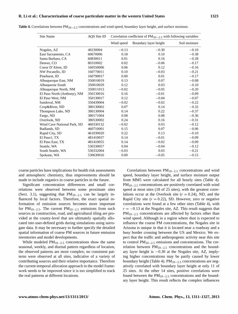
Table 4.Correlations between PM10−2.5 concentrations and wind speed, boundary layer height, and surface moisture.

Site Name AQS Site ID Correlation coefficient of PM10−2.5 with following variables

Wind speed Boundary layer height Soil moisture

Nogales, AZ 40230004 −0.13 −0.30 −0.10East Sacramento, CA 60670006 0.18 0.10 −0.38Santa Barbara, CA 60830011 0.01 0.16 −0.28Denver, CO 80310002 0.02 −0.06 −0.17Coeur D’Alene, ID 160550006 0.06 0.12 −0.16NW Pocatello, ID 160770011 0.10 −0.03 −0.21Pinehurst, ID 160790017 0.00 0.01 −0.17Albuquerque East, NM 350010019 0.13 0.07 −0.08Albuquerue South 350010029 0.12 0.03 −0.10Albuquerque North, NM 350011013 −0.02 −0.05 −0.20El Paso North (Anthony), NM 350130016 0.16 −0.01 −0.09El Paso West, NM 350130017 0.12 −0.04 −0.07Sandoval, NM 350439004 −0.02 −0.02 −0.22Crop&River, ND 380130002 0.07 0.14 −0.32Thompson Lake, ND 380130004 0.14 0.22 −0.37Fargo, ND 380171004 0.08 0.08 −0.36Overlook, ND 380530002 0.24 0.16 −0.31Wind Cave National Park, SD 460330132 −0.02 0.03 −0.12Badlands, SD 460710001 0.15 0.07 −0.06Rapid City, SD 461030020 0.22 0.13 −0.10El Paso1, TX 481410037 0.14 −0.01 −0.09El Paso East, TX 481410055 0.14 −0.02 −0.09Seattle, WA 530330057 0.04 −0.04 −0.12South Seattle, WA 530332004 −0.03 0.03 −0.21Spokane, WA 530630016 0.00 −0.05 −0.15

coarse particles have implications for health risk assessmentsand atmospheric chemistry, thus improvements should bemade to include organics in coarse particles in the future.

Significant concentration differences and small cor-relations were observed between some proximate sites(Sect. 3.1), suggesting that PM10−2.5 can be largely in-fluenced by local factors. Therefore, the exact spatial in-formation of emission sources becomes more importantfor PM10−2.5. The current PM10−2.5 emissions from suchsources as construction, road, and agricultural tiling are pro-vided at the county-level that are ultimately spatially allo-cated into user-defined grids during simulations using surro-gate data. It may be necessary to further specify the detailedspatial information of coarse PM sources in future emissioninventories and model developments.

While modeled PM10−2.5 concentrations show the sameseasonal, weekly, and diurnal pattern regardless of location,the observed patterns are more complex; no consistent pat-terns were observed at all sites, indicative of a variety ofcontributing sources and their relative importance. Thereforethe current temporal allocation approach in the model frame-work needs to be improved since it is too simplified to trackthe real patterns at different locations.

Correlations between PM10−2.5 concentrations and windspeed, boundary layer height, and surface moisture outputfrom MM5 were calculated for all hourly sites (Table 4).PM10−2.5 concentrations are positively correlated with windspeed at most sites (18 of 25 sites), with the greatest corre-lations occur at the Overlook site (r = 0.24), ND, and theRapid City site (r = 0.22), SD. However, zero or negativecorrelations were found at a few other sites (Table 4), withr = −0.13 at the Nogales site, AZ. This result suggests thatPM10−2.5 concentrations are affected by factors other thanwind speed. Although in a region where dust is expected toinfluence the coarse PM concentrations, the Nogales site inArizona is unique in that it is located near a roadway and abusy border crossing between the US and Mexico. We ex-pect that the traffic and anthropogenic activity near this siteto control PM10−2.5 emissions and concentrations. The cor-relation between PM10−2.5 concentrations and the bound-ary layer height is−0.30 at the Nogales site, AZ, imply-ing higher concentrations may be partly caused by lowerboundary height (Table 4). PM10−2.5 concentrations are neg-atively correlated with boundary layer height at only 11 of25 sites. At the other 14 sites, positive correlations werefound between the PM10−2.5 concentrations and the bound-ary layer height. This result reflects the complex influences



on PM10−2.5 concentrations by the boundary layer height andother possible factors as well as their interactions. PM10−2.5concentrations are negatively correlated with soil moisture atall investigated sites (Table 4), indicating that high PM10−2.5concentrations are correlated to lower soil moisture. Sinceless dust can be emitted into the atmosphere in wet condi-tions and airborne particles can be washed out at precipita-tion events, higher concentrations of dust are expected underdrier conditions.

Chemical and biological analyses of measured PM10−2.5can be employed to quantify percentage contributions fromdifferent sources at the ambient measurement sites; how-ever, little chemical or biological speciation data exists forPM10−2.5. By taking an approach that combines both massconcentration observations and model simulations, this studyhas improved our understanding of the sources and behaviorof PM10−2.5 concentrations at a regional scale in the westernUnited States, and has provided insights into future develop-ments of models that simulate atmospheric PM10−2.5 emis-sions, transport, and fate.

Measurement of all of criteria air pollutants is requiredby law. To help meet this requirement, a Federal ReferenceMethod (FRM) and Federal Equivalency Methods (FEM) foreach have been established and are documented in the Codeof Federal Regulations (CFR). The FRM and FEM require-ments are stringent with lengthy quality control and qualityassurance protocols for each pollutant. The end result is highquality measurement data for each pollutant being reportedin the AQS. AQS data have been used successfully by nu-merous studies (e.g. Chang et al., 2012; Drury et al., 2010;Jensen et al., 2009; Sampson et al., 2011; van Donkelaar etal., 2006; Zhang et al., 2006). FRM and FEM for PM10−2.5were not established until 2007 and, as such, there are noPM10−2.5 mass concentrations in the AQS for our study yearof 2005. The FRM for PM10−2.5 involves subtraction of lowvolume FRM PM2.5 mass concentration from a co-locatedlow volume FRM PM10 mass concentration (for more de-tails see CFR 40 Part 50 Appendix O). Our approach herewas to use the best possible substitute. We used subtrac-tion of collocated FRM PM2.5 mass concentration from FRMPM10 mass concentration, without distinction of sample vol-ume. This approach will likely increase the uncertainty as-sociated with the resulting PM10−2.5 mass concentrations ascompared to the FRM PM10−2.5. Additionally, this approachmay potentially introduce a small bias associated with howvolatile components are assessed. However, the magnitudeof the potential bias and uncertainty associated with our ap-proach is relatively small compared to the big differences be-tween measured and modeled PM10−2.5 concentrations (USEPA, 2004, 2009). In other words, the uncertainties of themeasurements cannot affect our conclusion that the modelingsystem significantly underpredicted PM10−2.5 concentrationsacross the western United States.

6 Summary and conclusion

We investigated the characteristics of observed coarse PMin the western US, and compared CMAQ predictions to theobservations. The observed concentrations showed a spatialpattern that could be explained in part with the distributionsof land use and soil moistures. The highest concentrationswere found in the southwestern US, where sparse vegeta-tion, open shrublands or barren lands dominate with lowersoil moistures, whereas the lowest concentrations occurredin areas dominated by grasslands, forest, or croplands withhigher soil moistures. Observed concentrations show differ-ent seasonal, weekly, and diurnal patterns at different loca-tions across the western United States, reflecting differentcontributing sources and their relative importance dependenton locations. CMAQ significantly under-predicted PM10−2.5concentrations. The under-prediction was likely due to omis-sion of sources such as pollen, bacteria, fungal spores, andespecially, geogenic dust, as well as under-estimation ofother significant source types. CMAQ also failed to repro-duce their spatial as well as seasonal, weekly, and diurnal pat-terns. Unlike observations, the modeled concentrations showsimilar seasonal, weekly, and diurnal pattern across the en-tire domain. CMAQ does not include organics in PM10−2.5,which recent measurements show to be a significant com-ponent. In this study we identified some important gaps forfuture developments of coarse PM models and emission in-ventories.

Acknowledgements.This work is supported by the US Environ-mental Protection Agency (STAR award # 834552). We thank NickMangus for his help with AQS data. Thanks also go to BradleyL. Rink for providing us with PM10 and PM2.5 data for the Denversite. The National Center for Atmospheric Research is operatedby the University Corporation for Atmospheric Research undersponsorship of the National Science Foundation.

Edited by: W. Birmili

References

Baldasano, J. M., Pay, M. T., Jorba, O., Gasso, S., and Jimenez-Guerrero, P.: An annual assessment of air quality with theCALIOPE modeling system over Spain, Sci. Total Environ., 409,2163–2178, 2011.

Birmili, W., Schepanski, K., Ansmann, A., Spindler, G., Tegen,I., Wehner, B., Nowak, A., Reimer, E., Mattis, I., Muller, K.,Bruggemann, E., Gnauk, T., Herrmann, H., Wiedensohler, A.,Althausen, D., Schladitz, A., Tuch, T., and Loschau, G.: A caseof extreme particulate matter concentrations over Central Europecaused by dust emitted over the southern Ukraine, Atmos. Chem.Phys., 8, 997–1016,doi:10.5194/acp-8-997-2008, 2008.

Boylan, J. W. and Russell, A. G.: PM and light extinction modelperformance metrics, goals, and criteria for three-dimensional airquality models, Atmos. Environ., 40, 4946–4959, 2006.


http://dx.doi.org/10.5194/acp-8-997-2008


Branis, M., Vyskovska, J., Maly, M., and Hovorka, J.: Associationof size-resolved number concentrations of particulate matter withcardiovascular and respiratory hospital admissions and mortalityin Prague, Czech Republic, Inhal. Toxicol., 22, 21–28, 2010.

Brunekreef, B. and Forsberg, B.: Epidemiological evidence of ef-fects of coarse airborne particles on health, Eur. Resp. J., 26,309–318, 2005.

Byun, D. W. and Schere, K. L.: Review of the governing equations,computational algorithms, and other components of the Models-3 Community Multiscale Air Quality (CMAQ) modeling system,Appl. Mech. Rev., 56, 51–77, 2006.

Carlton, A. G., Turpin, B. J., Altieri, K. E., Seitzinger, S. P., Mathur,R., Roselle, S. J., and Weber, R. J.: CMAQ model performanceenhanced when in-cloud secondary organic aerosol is included:Comparisons of organic carbon predictions with measurements,Environ. Sci. Technol., 42, 8798–8802, 2008.

Carlton, A. G., Bhave, P. V., Napelenok, S. L., Edney, E. D., Sarwar,G., Pinder, R. W., Pouliot, G. A., and Houyoux, M.: Model rep-resentation of secondary organic aerosol in CMAQv4.7, Environ.Sci. Technol., 44, 8553–8560, 2010.

Chang, H. H., Reich, B. J., and Miranda, M. L.: Time-to-eventanalysis of fine particle air pollution and preterm birth: resultsfrom North Carolina, 2001–2005, Am. J. Epidemiol., 175, 91–98, 2012.

Cheung, K., Daher, N., Kam, W., Shafer, M. M., Ning, Z., Schauer,J. J., and Sioutas, C.: Spatial and temporal variation of chemi-cal composition and mass closure of ambient coarse particulatematter (PM10−2.5) in the Los Angeles area, Atmos. Environ., 45,2651–2662, 2011.

Chuang, M., Zhang, Y., and Kang, D.: Application of WRF/Chem-MADRID for real-time air quality forecasting over the southeast-ern United States, Atmos. Environ., 45, 6241–6250, 2011.

Clements, N., Piedrahita, R., Ortega, J., Peel, J. L., Hannigan,M., Miller, S. L., and Milford, J. B.: Characterization and non-parametric regression of rural and urban coarse particulate mat-ter mass concentrations in northeastern Colorado, Aerosol. Sci.Technol., 46, 108–123, 2012.

DeMott, P., Sassen, K., Poellot, M., Baumgardner, D., Rogers,D., Brooks, S., Prenni, A., and Kreidenweis, S.: African dustaerosols as atmospheric ice nuclei, Geophys. Res. Lett., 30, 1732,doi:10.1029/2003GL017410, 2003.

Drury, E., Jacob, D. J., Spurr, R. J. D., Wang, J., Shinozuka,Y., Anderson, B. E., Clarke, A. D., Dibb, J., McNaughton,C., and Weber, R.: Synthesis of satellite (MODIS), aircraft(ICARTT), and surface (IMPROVE, EPA-AQS, AERONET)aerosol observations over eastern North America to improveMODIS aerosol retrievals and constrain surface aerosol concen-trations and sources, J. Geophys. Res.-Atmos., 115, D14204,doi:10.1029/2009JD012629, 2010.

Dudhia, J.: Numerical study of convection observed during thewinter monsoon experiment using a mesoscale two-dimensionalmodel, J. Atmos. Sci., 46, 3077–3107, 1989.

Edgerton, E. S., Casuccio, G. S., Saylor, R. D., Lersch, T. L., Hart-sell, B. E., Jansen, J. J., and Hansen, D. A.: Measurements of OCand EC in coarse particulate matter in the southeastern UnitedStates, J. Air Waste Manage., 59, 78–90, 2009.

Foley, K. M., Roselle, S. J., Appel, K. W., Bhave, P. V., Pleim, J.E., Otte, T. L., Mathur, R., Sarwar, G., Young, J. O., Gilliam,R. C., Nolte, C. G., Kelly, J. T., Gilliland, A. B., and Bash, J.

O.: Incremental testing of the Community Multiscale Air Quality(CMAQ) modeling system version 4.7, Geosci. Model Dev., 3,205–226,doi:10.5194/gmd-3-205-2010, 2010.

Harrison, R. M., Yin, J. X., Mark, D., Stedman, J., Appleby, R. S.,Booker, J., and Moorcroft, S.: Studies of the coarse particle (2.5–10 µm) component in UK urban atmospheres, Atmos. Environ.,35, 3667–3679, 2001.

Host, S., Larrieu, S., Pascal, L., Blanchard, M., Declercq, C., Fabre,P., Jusot, J., Chardon, B., Le Tertre, A., Wagner, V., Prouvost, H.,and Lefranc, A.: Short-term associations between fine and coarseparticles and hospital admissions for cardiorespiratory diseasesin six French cities, Occup. Environ. Med., 65, 544–551, 2008.

Houyoux, M., Vukovich, J., Coats, C., Wheeler, N., and Kasibhatla,P.: Emission inventory development and processing for the Sea-sonal Model for Regional Air Quality (SMRAQ) project, J. Geo-phys. Res.-Atmos., 105, 9079–9090, 2000.

Jensen, S. S., Larson, T., Deepti, K. C., and Kaufman, J. D.: Mod-eling traffic air pollution in street canyons in New York City forintra-urban exposure assessment in the US Multi-Ethnic Studyof atherosclerosis and air pollution, Atmos. Environ., 43, 4544–4556, 2009.

Kain, J.: The Kain-Fritsch convective parameterization: an update,J. Appl. Meteorol., 43, 170–181, 2004.

Kelly, J. T., Bhave, P. V., Nolte, C. G., Shankar, U., and Foley, K.M.: Simulating emission and chemical evolution of coarse sea-salt particles in the Community Multiscale Air Quality (CMAQ)model, Geosci. Model Dev., 3, 257–273,doi:10.5194/gmd-3-257-2010, 2010.

Koehler, K. A., Kreidenweis, S. M., DeMott, P. J., Petters, M. D.,Prenni, A. J., and Carrico, C. M.: Hygroscopicity and clouddroplet activation of mineral dust aerosol, Geophys. Res. Lett.,36, L08805,doi:10.1029/2009GL037348, 2009.

Konovalov, I. B., Beekmann, M., Kuznetsova, I. N., Yurova, A., andZvyagintsev, A. M.: Atmospheric impacts of the 2010 Russianwildfires: integrating modelling and measurements of an extremeair pollution episode in the Moscow region, Atmos. Chem. Phys.,11, 10031–10056,doi:10.5194/acp-11-10031-2011, 2011.

Krueger, B., Grassian, V., Cowin, J., and Laskin, A.: Heterogeneouschemistry of individual mineral dust particles from different dustsource regions: the importance of particle mineralogy, Atmos.Environ., 38, 6253–6261, 2004.

Kumar, P., Nenes, A., and Sokolik, I. N.: Importance of ad-sorption for CCN activity and hygroscopic properties ofmineral dust aerosol, Geophys. Res. Lett., 36, L24804,doi:10.1029/2009GL040827, 2009.

Kumar, P., Sokolik, I. N., and Nenes, A.: Measurements of cloudcondensation nuclei activity and droplet activation kinetics offresh unprocessed regional dust samples and minerals, Atmos.Chem. Phys., 11, 3527–3541,doi:10.5194/acp-11-3527-2011,2011.

Lagudu, U. R. K., Raja, S., Hopke, P. K., Chalupa, D. C., Utell, M.J., Casuccio, G., Lersch, T. L., and West, R. R.: Heterogeneityof coarse particles in an urban area, Environ. Sci. Technol., 45,3288–3296, 2011.

Lonati, G., Pirovano, G., Sghirlanzoni, G. A., and Zanoni, A.: Spe-ciated fine particulate matter in northern Italy: A whole yearchemical and transport modelling reconstruction, Atmos. Res.,95, 496–514, 2010.


http://dx.doi.org/10.1029/2003GL017410

http://dx.doi.org/10.1029/2009JD012629

http://dx.doi.org/10.5194/gmd-3-205-2010



http://dx.doi.org/10.1029/2009GL037348


http://dx.doi.org/10.1029/2009GL040827



Mahowald, N.: Aerosol indirect effect on biogeochemical cyclesand climate, Science, 334, 794–796, 2011.

Malig, B. J. and Ostro, B. D.: Coarse particles and mortality: ev-idence from a multi-city study in California, Occup. Environ.Med., 66, 832–839, 2009.

Malm, W. C., Pitchford, M. L., McDade, C., and Ashbaugh, L. L.:Coarse particle speciation at selected locations in the rural conti-nental United States, Atmos. Environ., 41, 2225–2239, 2007.

Mlawer, E., Taubman, S., Brown, P., Iacono, M., and Clough, S.:Radiative transfer for inhomogeneous atmospheres: RRTM, avalidated correlated-k model for the longwave, J. Geophys. Res.-Atmos., 102, 16663–16682, 1997.

Nenes, A., Pandis, S., and Pilinis, C.: Continued development andtesting of a new thermodynamic aerosol module for urban andregional air quality models, Atmos. Environ., 33, 1553–1560,1999.

Otte, T. L. and Pleim, J. E.: The Meteorology-Chemistry Inter-face Processor (MCIP) for the CMAQ modeling system: up-dates through MCIPv3.4.1, Geosci. Model Dev., 3, 243–256,doi:10.5194/gmd-3-243-2010, 2010.

Pakbin, P., Hudda, N., Cheung, K. L., Moore, K. F., and Sioutas,C.: Spatial and temporal variability of coarse (PM10−2.5) par-ticulate matter concentrations in the Los Angeles area, Aerosol.Sci. Technol., 44, 514–525, 2010.

Paytan, A., Mackey, K. R. M., Chen, Y., Lima, I. D., Doney, S.C., Mahowald, N., Labiosa, R., and Postf, A. F.: Toxicity of at-mospheric aerosols on marine phytoplankton, P. Natl. Acad. Sci.USA, 106, 4601–4605, 2009.

Perez, L., Tobias, A., Querol, X., Kunzli, N., Pey, J., Alastuey,A., Viana, M., Valero, N., Gonzalez-Cabre, M., and Sunyer, J.:Coarse particles from Saharan dust and daily mortality, Epidemi-ology, 19, 800–807, 2008.

Pierce, T., Geron, C., Bender, L., Dennis, R., Tonnesen, G., andGuenther, A.: Influence of increased isoprene emissions on re-gional ozone modeling, J. Geophys. Res.-Atmos., 103, 25611–25629, 1998.

Pleim, J. E. and Xiu, A. J.: Development of a land surface model.Part II: data assimilation, J. Appl. Meteorol., 42, 1811–1822,2003.

Reisner, J., Rasmussen, R., and Bruintjes, R.: Explicit forecastingof supercooled liquid water in winter storms using the MM5mesoscale model, Q. J. R. Meteorol. Soc., 124, 1071–1107,1998.

Sampson, P. D., Szpiro, A. A., Sheppard, L., Lindstrom, J., andKaufman, J. D.: Pragmatic estimation of a spatio-temporal airquality model with irregular monitoring data, Atmos. Environ.,45, 6593–6606, 2011.

Sandstrom, T. and Forsberg, B.: Desert dust: an unrecognizedsource of dangerous air pollution?, Epidemiology, 19, 808–809,2008.

Sarwar, G., Luecken, D., Yarwood, G., Whitten, G. Z., and Carter,W. P. L.: Impact of an updated carbon bond mechanism on pre-dictions from the CMAQ modeling system: preliminary assess-ment, J. Appl. Meteorol. Clim., 47, 3–14, 2008.

Sesartic, A. and Dallafior, T. N.: Global fungal spore emissions, re-view and synthesis of literature data, Biogeosciences, 8, 1181–1192,doi:10.5194/bg-8-1181-2011, 2011.

Sokhi, R. S., Mao, H., Srimath, S. T. G., Fan, S., Kitwiroon, N.,Luhana, L., Kukkonen, J., Haakana, M., Karppinen, A., van den

Hout, K. D., Boulter, P., McCrae, I. S., Larssen, S., Gjerstad,K. I., Jose, R. S., Bartzis, J., Neofytou, P., van den Breerner, P.,Neville, S., Kousa, A., Cortes, B. M. and Myrtveit, I.: An inte-grated multi-model approach for air quality assessment: devel-opment and evaluation of the OSCAR Air Quality AssessmentSystem, Environ. Modell. Softw., 23, 268–281, 2008.

Solomon, S., Qin, D., Manning, M., Chen, Z., Marquis, M., Averyt,K. B., Tignor, M., and Miller, H. L. (Eds.): Climate Change 2007:The Physical Science Basis. Contribution of Working Group Ito the Fourth Assessment Report of the Intergovernmental Panelon Climate Change (IPCC), Cambridge University Press, Cam-bridge, United Kingdom, 2007.

Textor, C., Schulz, M., Guibert, S., Kinne, S., Balkanski, Y., Bauer,S., Berntsen, T., Berglen, T., Boucher, O., Chin, M., Dentener, F.,Diehl, T., Easter, R., Feichter, H., Fillmore, D., Ghan, S., Ginoux,P., Gong, S., Grini, A., Hendricks, J., Horowitz, L., Huang, P.,Isaksen, I., Iversen, I., Kloster, S., Koch, D., Kirkevag, A., Krist-jansson, J. E., Krol, M., Lauer, A., Lamarque, J. F., Liu, X., Mon-tanaro, V., Myhre, G., Penner, J., Pitari, G., Reddy, S., Seland,Ø., Stier, P., Takemura, T., and Tie, X.: Analysis and quantifica-tion of the diversities of aerosol life cycles within AeroCom, At-mos. Chem. Phys., 6, 1777–1813,doi:10.5194/acp-6-1777-2006,2006.

Thornburg, J., Rodes, C. E., Lawless, P. A., and Williams, R.: Spa-tial and temporal variability of outdoor coarse particulate mattermass concentrations measured with a new coarse particle sam-pler during the Detroit Exposure and Aerosol Research Study,Atmos. Environ., 43, 4251–4258, 2009.

US EPA: Air Quality Criteria for Particulate Matter, US En-vironmental Protection Agency, Research Triangle Park, NC,EPA/600/P-99/002aF-bF, 2004.

US EPA: Integrated Science Assessment for Particulate Matter (Fi-nal Report), EPA/600/R-08/139F, US Environmental ProtectionAgency, Washington, DC, 2009.

van Donkelaar, A., Martin, R. V., and Park, R. J.: Estimatingground-level PM2.5 using aerosol optical depth determined fromsatellite remote sensing, J. Geophys. Res.-Atmos., 111, D21201,doi:10.1029/2005JD006996, 2006.

Wang, L., Hao, J., He, K., Wang, S., Li, J., Zhang, Q., Streets, D. G.,Fu, J. S., Jang, C. J., Takekawa, H., and Chatani, S.: A modelingstudy of coarse particulate matter pollution in Beijing: regionalsource contributions and control implications for the 2008 sum-mer Olympics, J. Air Waste Manage., 58, 1057–1069, 2008.

Wang, Y., Zhuang, G., Tang, A., Zhang, W., Sun, Y., Wang, Z., andAn, Z.: The evolution of chemical components of aerosols at fivemonitoring sites of China during dust storms, Atmos. Environ.,41, 1091–1106, 2007.

Whitten, G. Z., Heo, G., Kimura, Y., McDonald-Buller, E., Allen, D.T., Carter, W. P. L., and Yarwood, G.: A new condensed toluenemechanism for Carbon Bond CB05-TU, Atmos. Environ., 44,5346–5355, 2010.

Wilson, W. and Suh, H.: Fine particles and coarse particles: con-centration relationships relevant to epidemiologic studies, J. AirWaste Manage., 47, 1238–1249, 1997.

Wurzler, S., Reisin, T., and Levin, Z.: Modification of mineral dustparticles by cloud processing and subsequent effects on drop sizedistributions, J. Geophys. Res.-Atmos., 105, 4501–4512, 2000.

Xiu, A. J. and Pleim, J. E.: Development of a land surface model.Part I: application in a mesoscale meteorological model, J. Appl.



http://dx.doi.org/10.5194/bg-8-1181-2011


http://dx.doi.org/10.1029/2005JD006996


Meteorol., 40, 192–209, 2001.Zanobetti, A. and Schwartz, J.: The effect of fine and coarse par-

ticulate air pollution on mortality: a national analysis, Environ.Health Perspect., 117, 898–903, 2009.

Zhang, J. F., Hu, W., Wei, F. S., Wu, G. P., Korn, L. R., and Chap-man, R. S.: Children’s respiratory morbidity prevalence in rela-tion to air pollution in four Chinese cities, Environ. Health Per-spect., 110, 961–967, 2002.

Zhang, Y., Liu, P., Queen, A., Misenis, C., Pun, B., Seigneur, C.,and Wu, S.: A comprehensive performance evaluation of MM5-CMAQ for the summer 1999 southern oxidants study episode –Part II: gas and aerosol predictions, Atmos. Environ., 40, 4839–4855, 2006.

Zhu, D., Kuhns, H. D., Brown, S., Gillies, J. A., Etyemezian, V., andGertler, A. W.: Fugitive dust emissions from paved road travelin the Lake Tahoe basin, J. Air Waste Manage., 59, 1219–1229,2009.


Characterization of coarse particulate matter in the ... · Characterization of coarse particulate...

Documents

Transcript of Characterization of coarse particulate matter in the ... · Characterization of coarse particulate...