Characterization of â-Amino Ester Enolates as Hexamers via 6Li NMRSpectroscopy

Anne J. McNeil,† Gilman E. S. Toombes,‡ Sithamalli V. Chandramouli,§ Benoit J. Vanasse,§Timothy A. Ayers,§ Michael K. O’Brien,§ Emil Lobkovsky,† Sol M. Gruner,‡ John A. Marohn,† and

David B. Collum*,†

Department of Chemistry and Chemical Biology, Baker Laboratory, Cornell UniVersity,Ithaca, New York 14853-1301, Physics Department, Clark Hall, Cornell UniVersity, Ithaca, New York 14853-2501,

and AVentis, Process DeVelopment Chemistry, Bridgewater, New Jersey 08807

Received February 11, 2004; E-mail: dbc6@cornell.edu

As part of a program to prepare new antithrombotic agents, wediscovered that unprotectedâ-amino esters can be exclusivelyC-alkylated. We sought to optimize this process by studying thestructures and reactivities ofâ-amino ester enolates.1 Determiningthe aggregation state of an enolate, however, is especially difficultdue to the high symmetry of the possible aggregatessmonomers,dimers, tetramers, and hexamerssand the spectroscopically opaqueLi-O linkage.2 Herein we describe a spectroscopic method usedto assignâ-amino ester enolates (1) as hexamers in solution.

To understand these studies we must briefly digress by describingthe dynamic phenomena that are commonly observed for organo-lithium aggregates but may seem surprising to the nonspecialist.3

At the lowest attainable NMR probe temperatures (<-100 °C),fast processes including solvent exchange,4 conformational equi-libria,5 and chelate isomerizations6 can become observable on NMRspectroscopic time scales, with concomitant spectral complexity.The spectra typically simplify on warming above-100 °C due totime averaging. Further warming of the probe often leads to aparticularly odd effect in whichintra-aggregate exchanges of6Linuclei become fast, whereasinter-aggregate exchanges are stillslow.7 Consequently, aggregates that differ by virtue of theiraggregation numbers (dimers versus hexamers) or subunit composi-tion (4:2 versus 3:3 mixed hexamers) appear as separate speciesby 6Li NMR spectroscopy, buteach aggregate manifests a single6Li resonance.This combination of rapidintra-aggregate exchangein conjunction with slowinter-aggregate exchange proves criticalto the structural assignments.

The 6Li NMR spectrum recorded on [6Li]( R)-1 in 9.0 M THF/toluene at-100°C shows a single resonance, consistent with almostany aggregation state of high symmetry. The6Li NMR spectrumrecorded on [6Li] rac-1 affords a single resonance at a markedlydifferent chemical shift than [6Li]( R)-1, suggesting the formationof a highly symmetricheterochiralaggregate. Partially racemic

mixtures using combinations of [6Li]( R)-1 and [6Li]( S)-1 at -100°C (Figure 1A) show both resonances along with considerable“noise” in the baseline. Additionally,6Li spectra recorded on [6-Li,15N](S)-1 and [6Li,15N]rac-1 show 6Li-15N coupling (d,JLi-N

) 3.4 and 3.6 Hz, respectively), confirming chelation as drawn.8

Varying the probe temperature from-100 to-50 °C affordeda single sharp resonance for [6Li]( R)-1, offering no evidence oflatent stereoisomerism, lower symmetry, or related structuralcomplexity. Conversely, warming samples containing varyingproportions of [6Li]( R)-1 and [6Li]( S)-1 revealedtwo resonancesin lieu of the baseline noisesfour resonances in total (Figure 1B).The data are consistent with deep-seated structural complexitiesthat simplify by rapidintra-aggregate exchange at elevated tem-peratures. Furthermore, the relative intensities are independent ofthe enolate concentration (0.04-0.40 M) and the THF concentration(2.0-9.0 M), indicating that the four species are at the sameaggregation and solvation state.

We considered models based on homochiral aggregates (RN orSN) and heterochiral aggregates (RnSN-n). RnSN-n/RN-nSn andRN/SN refer to pairs of spectroscopically indistinguishable enantiomers.Dimers (R1S1 andR2/S2) and tetramers (R4/S4, R1S3/R3S1, andR2S2)afford only two and three6Li resonances, respectively. Conversely,four discrete resonances are consistent with an ensemble of homo-and heterochiral hexamers:R6/S6, R1S5/R5S1, R2S4/R4S2, andR3S3.

A compelling picture emerges from a variant of a Job plot (Figure2) in which the intensities of the four resonances are plotted as afunction of the mole fraction of subunit (R)-1, XR.9 The maximumobserved for each aggregate coincides with the stoichiometry ofthe aggregate. The concentration dependencies were modeled asfollows.10,11

† Department of Chemistry and Chemical Biology, Cornell University.‡ Physics Department, Cornell University.§ Aventis.

Figure 1. 6Li NMR spectra recorded on a 0.2 M enolate mixture (50% ee)in 9.0 M THF/toluene at (A)-100°C and (B)-50°C: (blue)R3S3; (green)R2S4/R4S2; (black) R1S5/R5S1; (red) R6/S6.

XR )

∑n)0

N

n[RnSN-n]

∑n)0

N

N[RnSN-n]

Xn )[RnSN-n]

∑j)0

N

[RjSN-j]

Published on Web 04/27/2004

5938 9 J. AM. CHEM. SOC. 2004 , 126, 5938-5939 10.1021/ja049245s CCC: $27.50 © 2004 American Chemical Society

where

Xn, the mole fraction of the aggregate, is an implicit function ofXR andφn and may be solved by an iterative parametric method. Itis instructive to present the results in terms of the followingequilibria:

If the aggregate distribution is purely statistical (φ0 ) φ1 ) ... )φ6), thenK1 ) 0.05,K2 ) 0.30, andK3 ) 0.75. Least-squares fitsillustrated in Figure 2 yield substantially different values:K1 )1.0 ( 0.1 × 10-3, K2 ) 5.0 ( 0.3 × 10-3, andK3 ) 115 ( 3 ×10-3. From the relationship∆Gm ) -RT ln(Km/Kstatistical), we obtainthe deviations from statistical as follows:∆G1 ) 1.73( 0.04 kcal/mol, ∆G2 ) 1.82( 0.03 kcal/mol, and∆G3 ) 0.83( 0.01 kcal/mol. Therefore, the heterochiralR3S3 hexamer is markedly morestable than the alternative homo- and heterochiral combinations.

An X-ray crystal structure was obtained ofrac-1 showing aprismatic hexamer (R3S3) of S6 symmetry (Figure 3).12,13Consistentwith the spectroscopic studies, this aggregate would show a single6Li resonance. The crystallization of theR3S3 form is satisfying inlight of its relative stability in solution. The high stability of theR3S3 hexamer could influence the stereochemistry of alkylation viaan asymmetric amplification.14

Detailed mechanistic studies on the alkylation of theâ-aminoester enolates will be reported in due course. The spectroscopicstrategy described herein may prove general for assigning structuresof enolates and alkoxides. Last, we are reminded to be cautiousabout dismissing baseline noise.

Acknowledgment. We thank Prof. Benjamin Widom for helpfuldiscussions. A.J.M. and D.B.C. thank the National Institutes ofHealth for direct support of this work. G.E.S.T. and S.M.G. thankthe DOE for support (DE-FG02-97ER62443).

Supporting Information Available: Experimental details, spec-troscopic data, mathematical derivations (PDF), and X-ray crystal-lographic data (CIF). This material is available free of charge via theInternet at http://pubs.acs.org.

References

(1) Enolization was effected without N-lithiation using LiHMDS. Chan-dramouli, S. V.; O’Brien, M. K.; Powner, T. H. WO Patent 0040547,2000. See also: Czekaj, M.; Klein, S. I.; Guertin, K. R.; Gardner, C. J.;Zulli, A. L.; Pauls, H. W.; Spada, A. P.; Cheney, D. L.; Brown, K. D.;Colussi, D. J.; Chu, V.; Leadley, R. J.; Dunwiddie, C. T.Bioorg. Med.Chem. Lett.2002, 12, 1667-1670. Nagula, G.; Huber, V. J.; Lum, C.;Goodman, B. A.Org. Lett.2000, 2, 3527-3529. Myers, A. G.; Gleason,J. L.; Yoon, T.J. Am. Chem. Soc.1995, 117, 8488-8489.

(2) Solution studies of enolate aggregation: (a) Wang, D. Z.; Streitwieser,A. J. Org. Chem.2003, 68, 8936-8942 and references therein. (b)Jackman, L. M.; Bortiatynski, J.AdV. Carbanion Chem.1992, 1, 45-87.

(3) For reviews on Li NMR spectroscopy, see: Gu¨nther, H.J. Braz. Chem.1999, 10, 241-262. Gunther, H. InAdVanced Applications of NMR toOrganometallic Chemistry; Gielen, M., Willem, R., Wrackmeyer, B., Eds.;Wiley & Sons: New York, 1996; pp 247-290.

(4) For leading references, see: Lucht, B. L.; Collum, D. B.Acc. Chem. Res.1999, 32, 1035-1042.

(5) Remenar, J. F.; Lucht, B. L.; Kruglyak, D.; Romesberg, F. E.; Gilchirst,J. H.; Collum, D. B.J. Org. Chem.1997, 62, 5748-5754. Collum, D. B.Acc. Chem. Res.1993, 26, 227-234. Boche, G.; Fraenkel, G.; Cabral, J.;Harms, K.; van Eikema Hommes, N. J. R.; Lohrenz, J.; Marsch, M.;Schleyer, P. v. R.J. Am. Chem. Soc.1992, 114, 1562-1565.

(6) (a) Reich, H. J.; Goldenberg, W. S.; Sanders, A. W.; Jantzi, K. L.;Tzschucke, C. C.J. Am. Chem. Soc.2003, 125, 3509-3521 and referencestherein. (b) Aubrecht, K. B.; Lucht, B. L.; Collum, D. B.Organometallics1999, 18, 2981-2987.

(7) Bauer, W.; Griesinger, C.J. Am. Chem. Soc.1993, 115, 10871-10882.See also ref 6b.

(8) [15N](S)-1 and [15N]rac-1 were synthesized via the Arndt-Eistert ho-mologation: Podlech, J.; Seebach, D.Liebigs Ann.1995, 1217-1228.

(9) Job, P.Ann. Chim.1928, 9, 113-203. Gil, V. M. S.; Oliveira, N. C.J.Chem. Educ.1990, 67, 473-478.

(10) Widom, B.Statistical Mechanics: A Concise Introduction for Chemists;Cambridge University Press: New York, 2002.

(11) WhereµR andµS are the chemical potentials ofR andS, gP correspondsto the free energy of assembly for each permutation, andC is a constant.

(12) rac-1 (0.20 M) was crystallized from a 9.0 M THF/toluene solution heldat -20 °C over 24 h.

(13) For more examples of ester enolate crystal structures, see: Williard, P.G. ComprehensiVe Organic Synthesis; Pergamon: New York, 1991; Vol.1, pp 1-47. Seebach, D.Angew Chem., Int. Ed. Engl.1988, 27, 1624-1654. Boche, G.; Langlotz, I.; Marsch, M.; Harms, K.Chem. Ber.1994,127, 2059-2064. Jastrzebski, J. T. B. H.; van Koten, G.; van de Mieroop,W. F. Inorg. Chim. Acta1988, 142, 169-171.

(14) Fenwick, D. R.; Kagan, H. B.Top. Stereochem.1999, 22, 257-296.

JA049245S

Figure 2. Job plot of the mole fraction ofRnS6-n/R6-nSn (Xn + X6-n) asa function of the mole fraction of theR enantiomer (XR) at -50 °C. For thecase wheren ) 3, onlyX3 is plotted. The best fit to the data is also shown:(blue) R3S3; (green)R2S4/R4S2; (black) R1S5/R5S1; (red) R6/S6.

[RnSN-n] ) CN!

n!(N - n)!φn exp(nµR + (N - n)µS

kT )

φn ) φN-n ) ⟨exp(-gP

kT )⟩

R3S3 y\zK1 1/2R6 + 1/2S6 K1 )

φ0

20φ3

R3S3 y\zK2 1/2R5S1 + 1/2R1S5 K2 )

3φ1

10φ3

R3S3 y\zK3 1/2R4S2 + 1/2R2S4 K3 )

3φ2

4φ3

Figure 3. ORTEP ofrac-1 revealing a hexameric aggregate ofS6 symmetry.Hydrogen atoms are omitted for clarity.

C O M M U N I C A T I O N S

J. AM. CHEM. SOC. 9 VOL. 126, NO. 19, 2004 5939

Characterization of β-Amino Ester Enolates as Hexamers via 6Li NMR Spectroscopy

 Anne J. McNeil,† Gilman E. S. Toombes,‡ Sithamalli V. Chandramouli,§ Benoit J. Vanasse,§

Timothy A. Ayers,§ Michael K. O’Brien,§ Emil Lobkovsky,† Sol M. Gruner,‡ John A. Marohn,† and David B. Collum*,†

†Department of Chemistry and Chemical Biology, Baker Laboratory, Cornell University, Ithaca, New York 14853-1301

‡Physics Department, Clark Hall, Cornell University, Ithaca, New York 14853-2501 §Aventis, Process Development Chemistry, Bridgewater, New Jersey, 08807

 Supporting Information

H3C O 3

OH2NLi

CH3 OCH3

OH2NLi

(R)-1 rac-1CH3 OCH3

OH2NLi

(S)-1CH

NMR Structural Studies I. 6Li NMR Spectra recorded on [6Li](R)-1, [6Li,15N](S)-1, [6Li]rac-1, and [6Li,15N]rac-1 in 9.8 M THF/cyclopentane at -90 oC. II. 6Li NMR Spectra recorded on [6Li](R)-1 (0.20 M) in 9.0 M THF/toluene at various temperatures. III. 6Li NMR Spectra recorded on [6Li]rac-1 (0.20 M) in 9.0 M THF/toluene at various temperatures. IV. 6Li NMR Spectra recorded on a mixture of [6Li](R)-1 (0.10 M) and [6Li]rac-1 (0.10 M) in 9.0 M THF/toluene at various temperatures. V. 6Li NMR Spectra recorded on a mixture of [6Li](R)-1 and [6Li]rac-1 (50 % ee) in 9.0 M THF/toluene at -50 oC at various enolate concentrations. VI. Plot of the mole fraction of the aggregate (Xn + X6-n) versus [enolate] for the spectra in section V. VII. Table of data for the plot in section VI. VIII. 6Li NMR Spectra recorded on a mixture of [6Li](R)-1 and [6Li]rac-1 (50 % ee) at -50 oC in various THF concentrations (toluene co-solvent). IX. Plot of the mole fraction of the aggregate (Xn + X6-n) versus [THF] for the spectra in section VIII. X. Table of data for the plot in section IX.

S1

XI. 6Li NMR Spectra recorded on mixtures of [6Li](S)-1 and [6Li]rac-1 at -50 oC in 9.0 M THF/toluene. XII. 6Li NMR Spectra recorded on mixtures of [6Li](R)-1 and [6Li]rac-1 at -50 oC in 9.0 M THF/toluene.  XIII. Plot of the mole fraction of the aggregate (Xn + X6-n) versus the mole fraction of R (XR) for the spectra in sections XI and XII. XIV. Table of data for the plot in section XIII.  Mathematical Derivations I. Introduction to the model. II. Boltzmann distribution. III. Multiplicity. IV. Chemical potential. V. The statistical case. VI. The parametric method. VII. Fitting the experimental data with the parametric method. VIII. Equilibrium constants. Crystal Structure Data I. Crystal structure: ORTEP. II. Crystal data and structure refinement. III. Table of bond lengths and angles.

S2

 

   I. 6Li NMR Spectra recorded in 9.8 M THF/cyclopentane at -90 oC: (A) [6Li](R)-1 (0.07 M); (B) [6Li,15N](S)-1 (0.13 M); (C) [6Li]rac-1 (0.13 M); (D) [6Li,15N]rac-1 (0.33 M).  

S3

  II. 6Li NMR Spectra recorded on [6Li](R)-1 (0.20 M) in 9.0 M THF/toluene: (A) -100 oC; (B) -75 oC; (C) -50 oC; (D) -25 oC; (E) 0 oC; (F) -90 oC after temperature series.

S4

  III. 6Li NMR Spectra recorded on [6Li]rac-1 (0.20 M) in 9.0 M THF/toluene: (A) -100 oC; (B) -75 oC; (C) -50 oC; (D) -25 oC; (E) 0 oC; (F) -90 oC after temperature series.

S5

  IV. 6Li NMR Spectra recorded on a mixture of [6Li](R)-1 (0.10 M) and [6Li]rac-1 (0.10 M) in 9.0 M THF/toluene: (A) -100 oC; (B) -75 oC; (C) -50 oC; (D) -25 oC; (E) 0 oC; (F) -90 oC after temperature series.  

S6

  V. 6Li NMR Spectra recorded on a mixture of [6Li](R)-1 and [6Li]rac-1 (50 % ee) in 9.0 M THF/toluene at -50 oC at various enolate concentrations: (A) 0.04 M; (B) 0.10 M; (C) 0.15 M; (D) 0.25 M; (E) 0.40 M. ( ) R3S3; ( ) R4S2/R2S4; ( ) R5S1/R1S5; ( ) R6/S6. RnSN-n/RN-nSn and RN/SN refer to pairs of spectroscopically indistinguishable enantiomers.  

S7

  VI. Plot of the mole fraction of the aggregate (Xn + X6-n) versus [enolate] for the spectra in section V. For the case where n = 3, only X3 is plotted. ( ) R3S3; ( ) R4S2/R2S4; ( ) R5S1/R1S5; ( ) R6/S6.   VII. Table of data for the plot in section VI. ([6Li](R)-1 and [6Li]rac-1 (50 % ee) in 9.0 M THF/toluene at -50 oC.)

[enolate] (M) R3S3 R4S2/R2S4 R5S1/R1S5 R6/S60.04 0.29 ± 0.01 0.32 ± 0.02 0.13 ± 0.01 0.26 ± 0.01 0.10 0.30 ± 0.01 0.30 ± 0.02 0.13 ± 0.01 0.27 ± 0.03 0.15 0.29 ± 0.01 0.31 ± 0.01 0.12 ± 0.01 0.28 ± 0.01 0.25 0.28 ± 0.02 0.30 ± 0.01 0.12 ± 0.01 0.296 ± 0.004 0.40 0.285 ± 0.002 0.30 ± 0.01 0.120 ± 0.003 0.30 ± 0.02

S8

  VIII. 6Li NMR Spectra recorded on a mixture of [6Li](R)-1 and [6Li]rac-1 (50 % ee) in various THF concentrations (toluene co-solvent) at -50 oC: (A) 2.0 M; (B) 4.0 M; (C) 6.0 M; (D) 8.0 M. ( ) R3S3; ( ) R4S2/R2S4; ( ) R5S1/R1S5; ( ) R6/S6.  

S9

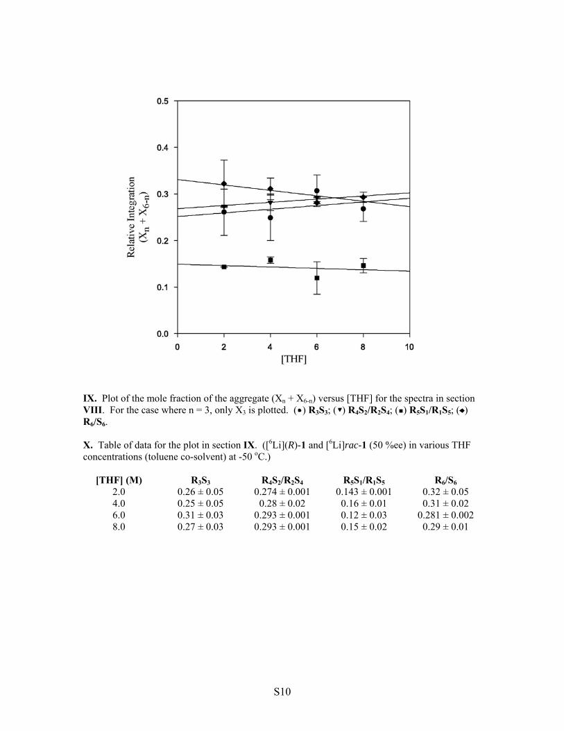
  IX. Plot of the mole fraction of the aggregate (Xn + X6-n) versus [THF] for the spectra in section VIII. For the case where n = 3, only X3 is plotted. ( ) R3S3; ( ) R4S2/R2S4; ( ) R5S1/R1S5; ( ) R6/S6. X. Table of data for the plot in section IX. ([6Li](R)-1 and [6Li]rac-1 (50 %ee) in various THF concentrations (toluene co-solvent) at -50 oC.)

[THF] (M) R3S3 R4S2/R2S4 R5S1/R1S5 R6/S62.0 0.26 ± 0.05 0.274 ± 0.001 0.143 ± 0.001 0.32 ± 0.05 4.0 0.25 ± 0.05 0.28 ± 0.02 0.16 ± 0.01 0.31 ± 0.02 6.0 0.31 ± 0.03 0.293 ± 0.001 0.12 ± 0.03 0.281 ± 0.002 8.0 0.27 ± 0.03 0.293 ± 0.001 0.15 ± 0.02 0.29 ± 0.01

S10

  XI. 6Li NMR Spectra recorded on mixtures of [6Li](S)-1 and [6Li]rac-1 ([enolate]total = 0.10 M) at -50 oC in 9.0 M THF/toluene: (A) ΧR = 0.0 ; (B) ΧR = 0.15; (C) ΧR = 0.25; (D) ΧR = 0.35; (E) ΧR = 0.45. ( ) R3S3; ( ) R4S2/R2S4; ( ) R5S1/R1S5; ( ) R6/S6.  

S11

  

  XII. 6Li NMR Spectra recorded on mixtures of [6Li](R)-1 and [6Li]rac-1 ([enolate]total = 0.10 M) at -50 oC in 9.0 M THF/toluene: (A) ΧR = 0.50 ; (B) ΧR = 0.55; (C) ΧR = 0.65; (D) ΧR = 0.75; (E) ΧR = 0.85; (F) ΧR = 1.0. ( ) R3S3; ( ) R4S2/R2S4; ( ) R5S1/R1S5; ( ) R6/S6.   

 

S12

XIII. Plot of the mole fraction of the aggregate (Xn + X6-n) versus the mole fraction of R (XR) for the spectra in sections XI and XII. For the case where n = 3, only X3 is plotted. ( ) R3S3; ( ) R4S2/R2S4; ( ) R5S1/R1S5; ( ) R6/S6. See “Mathematical Derivations” section VII for details of the fit. XIV. Table of data for the plot in section XIII. (0.10 M [enolate]total at -50 oC in 9.0 M THF/toluene.)

ΧR R3S3 R4S2/R2S4 R5S1/R1S5 R6/S60.00 0.00 ± 0.00 0.00 ± 0.00 0.00 ± 0.00 1.00 ± 0.00 0.15 0.13 ± 0.02 0.230 ± 0.001 0.14 ± 0.01 0.50 ± 0.02 0.25 0.32 ± 0.01 0.34 ± 0.03 0.10 ± 0.01 0.238 ± 0.003 0.35 0.51 ± 0.01 0.34 ± 0.02 0.06 ± 0.02 0.08 ± 0.03 0.40 0.72 ± 0.05 0.28 ± 0.05 0.00 ± 0.00 0.00 ± 0.00 0.50 0.79 ± 0.04 0.21 ± 0.04 0.00 ± 0.00 0.00 ± 0.00 0.55 0.75 ± 0.03 0.25 ± 0.03 0.00 ± 0.00 0.00 ± 0.00 0.65 0.48 ± 0.06 0.33 ± 0.01 0.09 ± 0.01 0.11 ± 0.03 0.75 0.29 ± 0.02 0.314 ± 0.001 0.13 ± 0.01 0.27 ± 0.01 0.85 0.133 ± 0.001 0.23 ± 0.01 0.15 ± 0.01 0.485 ± 0.001 1.00 0.00 ± 0.00 0.00 ± 0.00 0.00 ± 0.00 1.00 ± 0.00

 

S13

Mathematical Derivations 

I. Introduction: We consider a situation where the two enantiomers, (R)-1 and (S)-1, assemble in solution to form hexamers (N = 6). For an individual hexamer, each of the six positions in the assembly can be occupied by an (R)-1 or an (S)-1 (hereafter denoted as R and S, respectively). One way to describe a hexamer is by listing the occupant of each position – RSSRSR, RRRRRR, or RRSSRS for example. Rather than consider the concentration of each permutation, P, we can group them according to the number of R subunits in the hexamer, nP. The concentration, [RnSN-

n], of states for which nP = n is given by the Boltzmann distribution. It will depend on

1. Multiplicity (Mn) : The number of permutations of P for which nP = n. By example, RSRSRS and SRRSSR are just two of 20 permutations with nP = 3.

2. Free Energy (gP) : Each permutation may have a different energy of

assembly/association. For example, RRRSSS may be a much less stable permutation than RSRSRS.

3. Chemical Potential (µR and µS) : The total amount of R, [Rtotal], and S, [Stotal], will set

the chemical potentials and shift the likelihood of various states. If [Rtotal] >> [Stotal], for instance, then the [R1S5] will be much less likely than [R5S1].

In the experiment, the independent variable is the mole fraction of subunits of R, XR, and the dependent variables are linear combinations of the mole fraction of [RnSN-n], Xn. Thus, we wish to predict Xn as a function of XR for a given model. In Section II we use the Boltzmann distribution to give the value of [RnSN-n] in terms of free energies, multiplicity and chemical potential. In Section III we give an explicit form for the multiplicity. The relationship between chemical potentials and [Rtotal], [Stotal] (or XR and XS) is derived in Section IV. Section V considers the case where the free energies of assembly for all the permutations are equal (statistical case) for which a simple analytic result is possible. As there are no model parameters in the statistical case, the data either fits the model or the statistical assumption is invalid. The general case does not have a simple analytic solution. A parametric approach is described in Section VI. This numeric method allows one to compare the experimental and predicted populations, Xn, for a given set of free energies. We obtain the residual error after an iterative optimization of the free energies to fit the data, thus giving a measure of the model’s validity. Section VII describes the implementation of this approach. Section VIII relates free energies to equilibrium constants within the system.     

S14

II. Boltzmann Distribution: Consider a given permutation, P, with np subunits of type R and N-np monomers of type S. The Boltzmann distribution gives its equilibrium concentration as  

⎟⎟⎠

⎞⎜⎜⎝

⎛ −++−×=

kTnNng

CP SPRPp µµ )(exp][

 where C is a constant, gP is the free energy of assembly of P, µR is the chemical potential of R and µS is the chemical potential of S (Widom, B. Statistical Mechanics: A Concise Introduction for Chemists; Cambridge University Press: New York, 2002). Within the experiment, all states for which nP = n are indistinguishable. The concentration of permutations for which np = n is given by

( )

( )nnP

Pn

SR

nnP

PSR

nnPnNn

p

PP

kTgM

kTnNnC

kTg

kTnNnCPSR

=

==−

⎟⎠⎞

⎜⎝⎛ −××⎟

⎠⎞

⎜⎝⎛ −+

×=

⎟⎠⎞

⎜⎝⎛ −×⎟

⎠⎞

⎜⎝⎛ −+

×== ∑∑

;

;;

expexp

expexp][][

µµ

µµ

 where Mn is the multiplicity (number of permutations P where nP = n) and the average of free energy is taken over all states for which nP = n. It will be helpful for the remainder of the discussion to define some “effective” variables  

nnP

Pn

SR

PkTg

kTs

kTr

=

⎟⎠⎞

⎜⎝⎛ −=⎟

⎠⎞

⎜⎝⎛=⎟

⎠⎞

⎜⎝⎛=

;

expexpexp φµµ

 Substituting these into the above expression gives

)1(][ nNn

nnnNn srMCSR −− ××××= φ

Increasing the chemical potential of R increases the value of “r” and favors the [R6S0], [R5S1], etc. states. Increasing the chemical potential of S increases the value of “s” which then favors [R0S6], [R1S5], etc. φn describes the mean free energy of permutations in [RnSN-n]. Increasing φn favors [RnSN-n] as would be expected if those states have a low free energy. Not all values of φn are independent. The free energy of a permutation, P, and the free energy of one in which R and S have been exchanged are the same because the aggregates are enantiomers. This has the important consequence that

nNn −= φφ Furthermore, free energies can only be measured relative to the free energy of a reference state. For example, if free energies are measured relative to that of [R6S0] then φ0 = φ6 = 1. When N is even, N/2 of the values of φn are independent. For example, when N = 6, φ1 ,φ2, and φ3 are independent of each other.

S15

III. Multiplicity: The value of Mn can be directly obtained by an exhaustive grouping of all hexamer permutations.

Species n Mn - Number of permutations

Permutations

R0S6 0 1 SSSSSS R1S5 1 6 RSSSSS, SRSSSS, SSRSSS, SSSRSS,

SSSSRS, SSSSSR R2S4 2 15 RRSSSS, RSRSSS, RSSRSS, RSSSRS,

RSSSSR, SRRSSS, SRSRSS, SRSSRS, SRSSSR, SSRRSS, SSRSRS, SSRSSR,

SSSRRS, SSSRSR, SSSSRR R3S3 3 20 RRRSSS, RRSRSS, RRSSRS, RRSSSR,

RSRRSS, RSRSRS, RSRSSR, RSSRRS, RSSRSR, RSSSRR, + 10 other states with R

and S switched R4S2 4 15 SSRRRR, SRSRRR, SRRSRR, SRRRSR,

SRRRRS, RSSRRR, RSRSRR, RSRRSR, RSRRRS, RRSSRR, RRSRSR, RRSRRS,

RRRSSR, RRRSRS, RRRRSS R5S1 5 6 SRRRRR, RSRRRR, RRSRRR, RRRSRR,

RRRRSR, RRRRRS R6S0 6 1 RRRRRR

Alternatively, one can use Pascal’s triangle or the binomial theorem to achieve the general result

( ) !!!MtyMultiplici n nnN

N×−

== .

S16

IV. Chemical Potential: The experimental variables are the mole fractions of [RnSN-n], Xn, and the mole fraction of R, XR. Their relationships to C, r and s are described below.  Using eq 1 to compute [RnSN-n], the mole fraction Xn is given by

( )

( )⎟⎠⎞

⎜⎝⎛ −×

××

⎟⎠⎞

⎜⎝⎛ −×

××=

⎟⎠⎞

⎜⎝⎛××

⎟⎠⎞

⎜⎝⎛××

=××××

××××==

∑

∑∑∑

=

==

−

−

=−

−

kTjM

kTnM

srM

srM

srMC

srMC

SR

SRX

SRN

jjj

SRnn

N

j

j

jj

n

nn

N

j

jNjjj

nNnnn

N

jjNj

nNnn

µµφ

µµφ

φ

φ

φ

φ

exp

exp

)2(][

][

0

000

which is independent of the value of C. Permutations with [RnSN-n] contain n subunits of R and N-n subunits of S. Thus, the mole fraction of R, XR, is given by 

)3(

][

][

][][][

0

0

0

0

0

0

∑

∑

∑

∑

∑

∑

=

=

=

−

=

−

=−

=−

⎟⎠⎞

⎜⎝⎛×××

⎟⎠⎞

⎜⎝⎛×××

=××××

××××=

×

×=

+=

N

n

n

nn

N

n

n

nn

N

n

nNnnn

N

n

nNnnn

N

nnNn

N

nnNn

totaltotal

totalR

srMN

srMn

srMN

srMn

SRN

SRn

SRRX

φ

φ

φ

φ

All mole fractions depend only on the ratio r/s and φn, and XR is a strictly monotonic function of r/s. Thus, if the mole fraction, XR, and φn are known, eq 3 uniquely determines r/s. Knowing r/s, the value of any mole fraction, Xn, can be computed using eq 2. In the special “statistical” case there is a simple analytic form for r/s. This case is examined in Section V. For the general case, r/s is most easily determined numerically. A parametric approach is described in Sections VI and VII.

S17

V. The Statistical Case: Eq 3 can be considerably simplified if every permutation (RRSRRS, SRRRRR, etc.) has the same free energy. In this case, φn is independent of n so eq 3 simplifies to  

( )

( )∑

∑

∑

∑

∑

∑

=

−

=

−

=

−

=

−

=

−

=

−

××−

×

××−

×=

==

N

n

nNn

N

n

nNn

N

n

nNnn

N

n

nNnn

N

n

nNnnn

N

n

nNnnn

R

srnNn

NN

srnNn

Nn

srNM

srnM

srNM

srnMX

0

0

0

0

0

0

!!!

!!!

φ

φ

Using the Binomial expansion

( )∑=

− +=−

N

j

NjNj babajNj

N0

)(!!

!  

gives  

( )( )

)4(1

1

R

RN

N

R XX

sr

srr

srNsrrNX

−=↔

+=

+×+××

=−

 which is an explicit expression for r/s as a function of XR. Substituting eq 4 into eq 2 determines the concentration of any species in solution in terms of XR. The mole fraction of [RnSN-n], Xn, is equal to    

( )

( )( ) ( )

( ) ( ) nNR

nR

N

nNn

N

j

jNj

nNn

N

j

jNjjj

nNnnn

n

XXnNn

N

srsr

nNnN

srjNj

N

srnNn

N

srM

srMX

−

−

=

−

−

=

−

−

−××−

=

+×

×−

=××

−

××−

=××

×××=

∑∑

1!!

!

)5(!!

!

!!!

!!!

00φ

φ

S18

The experimental NMR signal measures linear combinations of Xn. For the specific case of N = 6,

Mole fraction of [R0S6] + [R6S0] = X0 + X6 Mole fraction of [R1S5] + [R5S1] = X1 + X5 Mole fraction of [R2S4] + [R4S2] = X2 + X4 Mole fraction of [R3S3] = X3

Using eq 5 these are equal to,

( )( ) ( )( ) ( )( )3R

3R33

4R

2R

2R

4R2442

5RRR

5R1551

6R

6R0660

X120X]S[RoffractionMole

X115XX115X]S[R]S[RoffractionMole

X16XX16X]S[R]S[RoffractionMole

X1X]S[R]S[RoffractionMole

−=

−+−=+

−+−=+

−+=+

The above formulae are used to plot all four populations as a function of XR. Because there are no free parameters, the experimental data either matches this plot, or the assumption that φn does not depend on n is wrong.

S19

VI. The Parametric Method: In general, each permutation can differ in stability, so φn depends on n. In this case, there is not a simple analytic expression for Xn as a function of XR and φn. However, eqs 2 and 3 permit one to evaluate XR and Xn as functions of r/s. For example, when N = 6, the total mole fraction of R is

)6(61520156

5101056

615

524

433

342

251

16

0

66

155

244

333

422

511

0

0

rsrsrsrsrsrsrsrsrsrsrsr

srNM

srnMX N

n

nNnnn

N

n

nNnnn

Rφφφφφφφ

φφφφφφ

φ

φ

+++++++++++

==

∑

∑

=

−

=

−

and the experimentally measured mole fractions, Xn, are

( )

( )

)10(61520156

20

)9(61520156

15

)8(61520156

6

)7(61520156

66

155

244

333

422

511

60

333

3

66

155

244

333

422

511

60

244

422

42

66

155

244

333

422

511

60

155

511

51

66

155

244

333

422

511

60

66

60

60

rsrsrsrsrsrssrX

rsrsrsrsrsrssrsrXX

rsrsrsrsrsrssrsrXX

rsrsrsrsrsrsrsXX

φφφφφφφφ

φφφφφφφφφ

φφφφφφφφφ

φφφφφφφφφ

++++++=

+++++++

=+

+++++++

=+

+++++++

=+

For a given value of XR and φn, one may determine the required value of r/s via numeric inversion of eq 6 or by graphing XR versus r. Using the obtained value r/s and eqs 7-10, one can then compute the populations. A graphical depiction of the parametric approach is described below for the case where φ0 = φ6 = 1, φ1 = φ5 = 1.5, φ2 = φ4 = 5, φ3 = 10. Since the above equations only depend on the ratio, r/s, for convenience we may define

rr

srrs

−=↔−=

11

S20

Using eq 6, we obtain the following plot for the example where φ0 = φ6 = 1, φ1 = φ5 = 1.5, φ2 = φ4 = 5, φ3 = 10.

The drop lines depicted for each XR allow one to determine the corresponding value of r. For this example we obtain the following values of r at each XR.

XR r r/s 0 0 0

0.1 0.0522 0.0551 0.2 0.104 0.116 0.3 0.175 0.213 0.4 0.296 0.421 0.5 0.50 1.0 0.6 0.704 2.377 0.7 0.825 4.706 0.8 0.896 8.643 0.9 0.948 18.14 1.0 1.0 infinity

S21

Using these values of r/s, we compute X0 + X6, X1 + X5, X2 + X4, and X3 using eqs 7-10. The results are plotted below.

( ) R3S3; ( ) R4S2/R2S4; ( ) R5S1/R1S5; ( ) R6/S6.

Comparing the above plot with the plot obtained in the statistical case (Section V), there are several notable changes. For instance, at XR = 0.5, R3S3 exhibits a maximum and is now the dominant species. This result matches our expectations because φ3 was set to be larger than all other φn’s (φ0 = φ6 = 1, φ1 = φ5 = 1.5, φ2 = φ4 = 5, φ3 = 10).

S22

VII. Fitting the Experimental Data with the Parametric Method: To compare the theory directly to experiment, one can refine an initial guess of φn until the predicted populations for the experimental values of XR best fit the experimental populations. An adaptive step algorithm iteratively adjusts φn to minimize the root mean square error in the predicted populations. N/2 of the φn variables are independent, and for N = 6, φ1, φ2, and φ3 are a convenient choice. A software package that supports nonlinear least-squares fitting of parametric equations is required.

( ) R3S3; ( ) R4S2/R2S4; ( ) R5S1/R1S5; ( ) R6/S6.

Best fit values of φ

φ0 φ1 φ2 φ3 φ4 φ5 φ61.0 0.79 7.3 47.7 7.3 0.79 1.0

Percent Errors in φn

n 0 1 2 3

φn/φo 0 3.7 6.5 9.4 φn/φ1 3.7 0 3.7 6.5 φn/φ2 6.5 3.7 0 2.8 φn/φ3 9.4 6.5 2.8 0

S23

VIII. Equilibrium Constants: The “free energy coefficients” φn, of RnSN-n, are related to the equilibrium constants as follows

R3S3 R6 S6+½

½

½

½ ½

½

R3S3

R3S3

R4S2 R2S4+

R5S1 R1S5+

K1

K2

K3

We now express K1, K2 and K3 in terms of φn using eq 1.

[ ] [ ][ ]33

2/16

2/16

1 SRSR ×

=K

Substituting the three concentrations into eq 1

 [ ] [ ] 33

33336

6666

006 ][ srMCSRrMCRsMCS ××××=×××=×××= φφφ which then give,

( ) ( )( ) 3

0

3333

2/1666

2/1600

1 20φφ

φφφ

=×

=srCM

rCMsCMK

For the above reactions,

3

23

3

12

3

01 4

3103

20 φφ

φφ

φφ

=== KKK

For the general case,

aRnSN-na abRnSN-nb b

cRnSN-nc cdRnSN-nd d

+ +K

( ) ( )( ) ( )bbnbn

aanan

ddndn

ccncn

MM

MMK

φφ

φφ

×

×=

 

S24

Kstatistical ∆Gstatistical

a (kcal/mol) K1 0.05 ∆G1 1.33 K2 0.30 ∆G2 0.53 K3 0.75 ∆G3 0.13

Kexperimental ∆Gnon-statisticalb (kcal/mol)

K1 1.0 ± 0.1 x 10-3 ∆G1 1.73 ± 0.04 K2 5.0 ± 0.3 x 10-3 ∆G2 1.82 ± 0.03 K3 115 ± 3 x 10-3 ∆G3 0.83 ± 0.01

a. ∆Gstatistical = - RTlnKstatistical where R = 0.001987 kcal/mol.K and T = 223.15 K. b. ∆Gnon-statistical = - RTlnKn/Kstatistical

S25

Crystal Structure   

  I. Crystals of rac-1 were obtained from a 0.20 M enolate solution in 9.0 M THF/toluene held at -20 oC over 24 h. Single crystals suitable for X-ray diffraction were coated with polyisobutylene oil in a glovebox and were quickly transferred to the goniometer head of a Siemens SMART (λ = 0.71073 A T=173 K). The crystal belongs to the space group P1(bar). 1818 frames were collected using 0.3 deg. omega scans (2θmax = 46.52 º). The data were processed with Bruker SAINT and SADABS programs to yield a total of 6120 unique reflections (R(int)=0.0575). The structure was solved using direct method (SHELXS) completed by subsequent Fourier synthesis and refined by full-matrix least-squares procedures (SHELXL). At final convergence, R(1) = 0.0665 for 3433 Fo > 4sig(Fo) and GOF = 0.949 for 772 parameters. .

  

S26

II. Crystal data and structure refinement.

Identification code am1

Empirical formula C15 H30 Li3 N3 O6

Formula weight 369.24

Temperature 173(2) K

Wavelength 0.71073 Å

Crystal system Triclinic

Space group P-1

Unit cell dimensions a = 13.423(11) Å α= 91.83(3)°.

b = 13.495(12) Å β= 104.60(2)°.

c = 13.817(12) Å γ = 111.29(3)°.

Volume 2235(3) Å3

Z 4

Density (calculated) 1.097 Mg/m3

Absorption coefficient 0.081 mm-1

F(000) 792

Crystal size 0.40 x 0.20 x 0.10 mm3

Theta range for data collection 1.63 to 23.26°.

Index ranges -13<=h<=14, -14<=k<=14, -14<=l<=15

Reflections collected 9964

Independent reflections 6120 [R(int) = 0.0575]

Completeness to theta = 23.26° 95.6 %

Absorption correction SADABS

Max. and min. transmission 0.9920 and 0.9684

Refinement method Full-matrix least-squares on F2

Data / restraints / parameters 6120 / 0 / 772

Goodness-of-fit on F2 0.949

Final R indices [I>2sigma(I)] R1 = 0.0665, wR2 = 0.1502

R indices (all data) R1 = 0.1275, wR2 = 0.1793

Largest diff. peak and hole 0.249 and -0.284 e.Å-3

S27

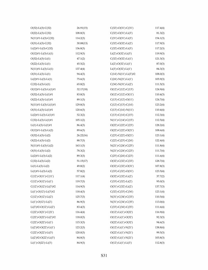
III. Table of Bond lengths [Å] and Angles [°]. O(11)‐C(12)   1.369(5) 

O(11)‐C(11)   1.414(6) 

O(12)‐C(12)   1.304(5) 

O(12)‐Li(3)#1   1.933(8) 

O(12)‐Li(1)   1.985(7) 

O(12)‐Li(2)   2.046(8) 

O(21)‐C(22)   1.366(5) 

O(21)‐C(21)   1.410(6) 

O(22)‐C(22)   1.294(5) 

O(22)‐Li(2)#1   1.915(7) 

O(22)‐Li(1)   1.946(7) 

O(22)‐Li(3)   2.031(8) 

O(31)‐C(32)   1.406(5) 

O(31)‐C(31)   1.429(5) 

O(31)‐Li(3)   2.557(7) 

O(32)‐C(32)   1.309(5) 

O(32)‐Li(3)   1.938(7) 

O(32)‐Li(2)   1.961(7) 

O(32)‐Li(1)   1.995(7) 

N(11)‐C(14)   1.474(6) 

N(11)‐Li(3)#1   2.086(8) 

N(21)‐C(24)   1.493(6) 

N(21)‐Li(1)   2.054(8) 

N(31)‐C(34)   1.506(6) 

N(31)‐Li(2)   2.038(8) 

C(12)‐C(13)   1.371(6) 

C(13)‐C(14)   1.501(6) 

C(14)‐C(15)   1.539(7) 

C(22)‐C(23)   1.341(6) 

C(22)‐Li(1)   2.766(8) 

C(23)‐C(24)   1.477(6) 

C(24)‐C(25)   1.532(6) 

C(32)‐C(33)   1.320(6) 

C(32)‐Li(3)   2.700(8) 

C(32)‐Li(2)   2.774(8) 

C(33)‐C(34)   1.531(6) 

C(34)‐C(35)   1.500(7) 

Li(1)‐Li(2)   2.712(10) 

Li(1)‐Li(3)   2.721(10) 

Li(1)‐Li(2)#1   3.307(10) 

Li(1)‐Li(3)#1   3.333(9) 

Li(2)‐O(22)#1   1.915(7) 

Li(2)‐Li(3)#1   2.677(9) 

Li(2)‐Li(1)#1   3.307(10) 

Li(2)‐Li(3)   3.502(9) 

Li(3)‐O(12)#1   1.933(8) 

Li(3)‐N(11)#1   2.086(8) 

Li(3)‐Li(2)#1   2.677(9) 

Li(3)‐Li(1)#1   3.333(9) 

O(11ʹ)‐C(12ʹ)   1.379(5) 

O(11ʹ)‐C(11ʹ)   1.411(5) 

O(12ʹ)‐C(12ʹ)   1.306(4) 

O(12ʹ)‐Li(1ʹ)   1.952(7) 

O(12ʹ)‐Li(3ʹ)#2   1.997(8) 

O(12ʹ)‐Li(2ʹ)   2.008(7) 

O(21ʹ)‐C(22ʹ)   1.428(5) 

O(21ʹ)‐C(21ʹ)   1.430(6) 

O(22ʹ)‐C(22ʹ)   1.305(5) 

O(22ʹ)‐Li(2ʹ)#2   1.957(8) 

O(22ʹ)‐Li(1ʹ)   1.977(7) 

O(22ʹ)‐Li(3ʹ)   1.994(7) 

O(31ʹ)‐C(32ʹ)   1.385(4) 

O(31ʹ)‐C(31ʹ)   1.421(6) 

O(31ʹ)‐Li(3ʹ)   2.660(7) 

O(32ʹ)‐C(32ʹ)   1.298(4) 

O(32ʹ)‐Li(2ʹ)   1.927(7) 

O(32ʹ)‐Li(3ʹ)   1.966(7) 

O(32ʹ)‐Li(1ʹ)   2.029(7) 

N(11ʹ)‐C(14ʹ)   1.513(5) 

N(11ʹ)‐Li(3ʹ)#2   2.045(7) 

N(21ʹ)‐C(24ʹ)   1.488(5) 

N(21ʹ)‐Li(1ʹ)   2.079(8) 

N(31ʹ)‐C(34ʹ)   1.480(6) 

N(31ʹ)‐Li(2ʹ)   2.060(8) 

C(12ʹ)‐C(13ʹ)   1.343(6) 

C(13ʹ)‐C(14ʹ)   1.483(6) 

C(14ʹ)‐C(15ʹ)   1.524(6) 

C(22ʹ)‐C(23ʹ)   1.328(6) 

C(23ʹ)‐C(24ʹ)   1.526(6) 

C(24ʹ)‐C(25ʹ)   1.501(7) 

C(32ʹ)‐C(33ʹ)   1.355(6) 

C(32ʹ)‐Li(2ʹ)   2.783(8) 

C(33ʹ)‐C(34ʹ)   1.481(6) 

C(34ʹ)‐C(35ʹ)   1.559(7) 

S28

Li(1ʹ)‐Li(3ʹ)   2.681(9) 

Li(1ʹ)‐Li(2ʹ)   2.725(10) 

Li(1ʹ)‐Li(3ʹ)#2   3.391(11) 

Li(1ʹ)‐Li(2ʹ)#2   3.461(10) 

Li(2ʹ)‐O(22ʹ)#2   1.957(8) 

Li(2ʹ)‐Li(3ʹ)#2   2.664(9) 

Li(2ʹ)‐Li(3ʹ)   3.369(9) 

Li(2ʹ)‐Li(1ʹ)#2   3.461(10) 

Li(3ʹ)‐O(12ʹ)#2   1.997(8) 

Li(3ʹ)‐N(11ʹ)#2   2.045(7) 

Li(3ʹ)‐Li(2ʹ)#2   2.664(9) 

Li(3ʹ)‐Li(1ʹ)#2   3.391(11) 

C(1S)‐C(2S)   0.90(5) 

C(1S)‐C(5S)#3   1.13(6) 

C(1S)‐C(4S)#3   1.61(6) 

C(1S)‐C(3S)   1.82(4) 

C(2S)‐C(3S)   1.111(18) 

C(2S)‐C(5S)#3   1.43(3) 

C(2S)‐C(5S)   1.62(3) 

C(3S)‐C(5S)   1.29(2) 

C(3S)‐C(4S)   1.90(3) 

C(4S)‐C(5S)   1.17(2) 

C(4S)‐C(1S)#3   1.61(6) 

C(5S)‐C(1S)#3   1.13(6) 

C(5S)‐C(2S)#3   1.43(3) 

C(5S)‐C(5S)#3   1.98(5) 

___________________________________________ 

C(12)‐O(11)‐C(11)  119.0(4) 

C(12)‐O(12)‐Li(3)#1  117.9(3) 

C(12)‐O(12)‐Li(1)  119.7(3) 

Li(3)#1‐O(12)‐Li(1)  116.6(3) 

C(12)‐O(12)‐Li(2)  123.8(3) 

Li(3)#1‐O(12)‐Li(2)  84.5(3) 

Li(1)‐O(12)‐Li(2)  84.6(3) 

C(22)‐O(21)‐C(21)  116.7(4) 

C(22)‐O(22)‐Li(2)#1  119.8(3) 

C(22)‐O(22)‐Li(1)  115.8(3) 

Li(2)#1‐O(22)‐Li(1)  117.9(3) 

C(22)‐O(22)‐Li(3)  123.3(3) 

Li(2)#1‐O(22)‐Li(3)  85.4(3) 

Li(1)‐O(22)‐Li(3)  86.3(3) 

C(32)‐O(31)‐C(31)  117.5(4) 

C(32)‐O(31)‐Li(3)  80.2(3) 

C(31)‐O(31)‐Li(3)  158.0(3) 

C(32)‐O(32)‐Li(3)  111.0(3) 

C(32)‐O(32)‐Li(2)  114.6(3) 

Li(3)‐O(32)‐Li(2)  127.9(3) 

C(32)‐O(32)‐Li(1)  124.8(3) 

Li(3)‐O(32)‐Li(1)  87.5(3) 

Li(2)‐O(32)‐Li(1)  86.6(3) 

C(14)‐N(11)‐Li(3)#1  108.4(3) 

C(24)‐N(21)‐Li(1)  107.8(4) 

C(34)‐N(31)‐Li(2)  105.0(3) 

O(12)‐C(12)‐O(11)  110.4(3) 

O(12)‐C(12)‐C(13)  126.1(4) 

O(11)‐C(12)‐C(13)  123.5(4) 

C(12)‐C(13)‐C(14)  122.7(4) 

N(11)‐C(14)‐C(13)  110.3(4) 

N(11)‐C(14)‐C(15)  112.1(4) 

C(13)‐C(14)‐C(15)  110.7(4) 

O(22)‐C(22)‐C(23)  127.6(4) 

O(22)‐C(22)‐O(21)  110.1(3) 

C(23)‐C(22)‐O(21)  122.3(4) 

O(22)‐C(22)‐Li(1)  39.3(2) 

C(23)‐C(22)‐Li(1)  95.1(3) 

O(21)‐C(22)‐Li(1)  136.2(3) 

C(22)‐C(23)‐C(24)  120.4(4) 

C(23)‐C(24)‐N(21)  110.2(4) 

C(23)‐C(24)‐C(25)  111.0(4) 

N(21)‐C(24)‐C(25)  112.6(4) 

O(32)‐C(32)‐C(33)  125.1(4) 

O(32)‐C(32)‐O(31)  109.5(3) 

C(33)‐C(32)‐O(31)  125.4(4) 

O(32)‐C(32)‐Li(3)  42.1(2) 

C(33)‐C(32)‐Li(3)  162.0(4) 

O(31)‐C(32)‐Li(3)  69.0(2) 

O(32)‐C(32)‐Li(2)  40.0(2) 

C(33)‐C(32)‐Li(2)  93.1(3) 

O(31)‐C(32)‐Li(2)  134.9(3) 

Li(3)‐C(32)‐Li(2)  79.6(2) 

C(32)‐C(33)‐C(34)  122.1(4) 

C(35)‐C(34)‐N(31)  111.8(4) 

C(35)‐C(34)‐C(33)  112.5(4) 

N(31)‐C(34)‐C(33)  109.8(4) 

O(22)‐Li(1)‐O(12)  124.2(3) 

O(22)‐Li(1)‐O(32)  93.5(3) 

S29

O(12)‐Li(1)‐O(32)  94.8(3) 

O(22)‐Li(1)‐N(21)  97.4(3) 

O(12)‐Li(1)‐N(21)  133.5(4) 

O(32)‐Li(1)‐N(21)  103.0(3) 

O(22)‐Li(1)‐Li(2)  117.8(4) 

O(12)‐Li(1)‐Li(2)  48.7(2) 

O(32)‐Li(1)‐Li(2)  46.2(2) 

N(21)‐Li(1)‐Li(2)  131.1(3) 

O(22)‐Li(1)‐Li(3)  48.1(2) 

O(12)‐Li(1)‐Li(3)  119.0(3) 

O(32)‐Li(1)‐Li(3)  45.4(2) 

N(21)‐Li(1)‐Li(3)  103.6(3) 

Li(2)‐Li(1)‐Li(3)  80.3(3) 

O(22)‐Li(1)‐C(22)  24.90(14) 

O(12)‐Li(1)‐C(22)  138.8(3) 

O(32)‐Li(1)‐C(22)  108.1(3) 

N(21)‐Li(1)‐C(22)  74.7(2) 

Li(2)‐Li(1)‐C(22)  142.0(3) 

Li(3)‐Li(1)‐C(22)  64.9(2) 

O(22)‐Li(1)‐Li(2)#1  30.78(18) 

O(12)‐Li(1)‐Li(2)#1  94.5(3) 

O(32)‐Li(1)‐Li(2)#1  88.3(3) 

N(21)‐Li(1)‐Li(2)#1  128.1(3) 

Li(2)‐Li(1)‐Li(2)#1  92.9(3) 

Li(3)‐Li(1)‐Li(2)#1  51.6(2) 

C(22)‐Li(1)‐Li(2)#1  53.88(19) 

O(22)‐Li(1)‐Li(3)#1  94.1(3) 

O(12)‐Li(1)‐Li(3)#1  31.24(18) 

O(32)‐Li(1)‐Li(3)#1  88.9(3) 

N(21)‐Li(1)‐Li(3)#1  162.8(4) 

Li(2)‐Li(1)‐Li(3)#1  51.3(2) 

Li(3)‐Li(1)‐Li(3)#1  93.6(3) 

C(22)‐Li(1)‐Li(3)#1  113.7(3) 

Li(2)#1‐Li(1)‐Li(3)#1  63.7(2) 

O(22)#1‐Li(2)‐O(32)  114.7(4) 

O(22)#1‐Li(2)‐N(31)  140.2(4) 

O(32)‐Li(2)‐N(31)  99.9(3) 

O(22)#1‐Li(2)‐O(12)  95.1(3) 

O(32)‐Li(2)‐O(12)  94.0(3) 

N(31)‐Li(2)‐O(12)  101.9(4) 

O(22)#1‐Li(2)‐Li(3)#1  49.1(2) 

O(32)‐Li(2)‐Li(3)#1  111.4(3) 

N(31)‐Li(2)‐Li(3)#1  134.8(4) 

O(12)‐Li(2)‐Li(3)#1  46.0(2) 

O(22)#1‐Li(2)‐Li(1)  112.6(3) 

O(32)‐Li(2)‐Li(1)  47.2(2) 

N(31)‐Li(2)‐Li(1)  105.2(3) 

O(12)‐Li(2)‐Li(1)  46.8(2) 

Li(3)#1‐Li(2)‐Li(1)  76.4(3) 

O(22)#1‐Li(2)‐C(32)  130.5(3) 

O(32)‐Li(2)‐C(32)  25.42(14) 

N(31)‐Li(2)‐C(32)  76.9(2) 

O(12)‐Li(2)‐C(32)  109.2(3) 

Li(3)#1‐Li(2)‐C(32)  136.5(3) 

Li(1)‐Li(2)‐C(32)  64.9(2) 

O(22)#1‐Li(2)‐Li(1)#1  31.32(18) 

O(32)‐Li(2)‐Li(1)#1  84.2(3) 

N(31)‐Li(2)‐Li(1)#1  166.6(4) 

O(12)‐Li(2)‐Li(1)#1  90.5(3) 

Li(3)#1‐Li(2)‐Li(1)#1  52.8(2) 

Li(1)‐Li(2)‐Li(1)#1  87.1(3) 

C(32)‐Li(2)‐Li(1)#1  104.1(2) 

O(22)#1‐Li(2)‐Li(3)  89.5(3) 

O(32)‐Li(2)‐Li(3)  25.89(17) 

N(31)‐Li(2)‐Li(3)  125.6(3) 

O(12)‐Li(2)‐Li(3)  90.5(3) 

Li(3)#1‐Li(2)‐Li(3)  90.7(3) 

Li(1)‐Li(2)‐Li(3)  50.0(2) 

C(32)‐Li(2)‐Li(3)  49.30(18) 

Li(1)#1‐Li(2)‐Li(3)  58.54(19) 

O(12)#1‐Li(3)‐O(32)  115.0(3) 

O(12)#1‐Li(3)‐O(22)  95.0(3) 

O(32)‐Li(3)‐O(22)  92.6(3) 

O(12)#1‐Li(3)‐N(11)#1  97.9(3) 

O(32)‐Li(3)‐N(11)#1  140.8(4) 

O(22)‐Li(3)‐N(11)#1  105.6(3) 

O(12)#1‐Li(3)‐O(31)  131.6(4) 

O(32)‐Li(3)‐O(31)  57.2(2) 

O(22)‐Li(3)‐O(31)  130.8(3) 

N(11)#1‐Li(3)‐O(31)  85.4(3) 

O(12)#1‐Li(3)‐Li(2)#1  49.5(2) 

O(32)‐Li(3)‐Li(2)#1  110.3(3) 

O(22)‐Li(3)‐Li(2)#1  45.5(2) 

N(11)#1‐Li(3)‐Li(2)#1  107.1(3) 

O(31)‐Li(3)‐Li(2)#1  167.4(3) 

O(12)#1‐Li(3)‐C(32)  131.7(3) 

S30

O(32)‐Li(3)‐C(32)  26.91(15) 

O(22)‐Li(3)‐C(32)  108.8(3) 

N(11)#1‐Li(3)‐C(32)  114.2(3) 

O(31)‐Li(3)‐C(32)  30.88(13) 

Li(2)#1‐Li(3)‐C(32)  136.8(3) 

O(12)#1‐Li(3)‐Li(1)  112.9(3) 

O(32)‐Li(3)‐Li(1)  47.1(2) 

O(22)‐Li(3)‐Li(1)  45.5(2) 

N(11)#1‐Li(3)‐Li(1)  137.4(4) 

O(31)‐Li(3)‐Li(1)  94.4(3) 

Li(2)#1‐Li(3)‐Li(1)  75.6(3) 

C(32)‐Li(3)‐Li(1)  65.8(2) 

O(12)#1‐Li(3)‐Li(1)#1  32.17(18) 

O(32)‐Li(3)‐Li(1)#1  83.8(3) 

O(22)‐Li(3)‐Li(1)#1  89.1(3) 

N(11)#1‐Li(3)‐Li(1)#1  129.8(3) 

O(31)‐Li(3)‐Li(1)#1  120.6(3) 

Li(2)#1‐Li(3)‐Li(1)#1  52.3(2) 

C(32)‐Li(3)‐Li(1)#1  105.1(2) 

Li(1)‐Li(3)‐Li(1)#1  86.4(3) 

O(12)#1‐Li(3)‐Li(2)  89.6(3) 

O(32)‐Li(3)‐Li(2)  26.22(16) 

O(22)‐Li(3)‐Li(2)  88.7(3) 

N(11)#1‐Li(3)‐Li(2)  163.1(3) 

O(31)‐Li(3)‐Li(2)  78.3(2) 

Li(2)#1‐Li(3)‐Li(2)  89.3(3) 

C(32)‐Li(3)‐Li(2)  51.15(17) 

Li(1)‐Li(3)‐Li(2)  49.8(2) 

Li(1)#1‐Li(3)‐Li(2)  57.8(2) 

C(12ʹ)‐O(11ʹ)‐C(11ʹ)  117.1(4) 

C(12ʹ)‐O(12ʹ)‐Li(1ʹ)  119.7(3) 

C(12ʹ)‐O(12ʹ)‐Li(3ʹ)#2  114.9(3) 

Li(1ʹ)‐O(12ʹ)‐Li(3ʹ)#2  118.4(3) 

C(12ʹ)‐O(12ʹ)‐Li(2ʹ)  125.7(3) 

Li(1ʹ)‐O(12ʹ)‐Li(2ʹ)  86.9(3) 

Li(3ʹ)#2‐O(12ʹ)‐Li(2ʹ)  83.4(3) 

C(22ʹ)‐O(21ʹ)‐C(21ʹ)  116.4(4) 

C(22ʹ)‐O(22ʹ)‐Li(2ʹ)#2  118.0(3) 

C(22ʹ)‐O(22ʹ)‐Li(1ʹ)  115.3(3) 

Li(2ʹ)#2‐O(22ʹ)‐Li(1ʹ)  123.2(3) 

C(22ʹ)‐O(22ʹ)‐Li(3ʹ)  120.0(3) 

Li(2ʹ)#2‐O(22ʹ)‐Li(3ʹ)  84.8(3) 

Li(1ʹ)‐O(22ʹ)‐Li(3ʹ)  84.9(3) 

C(32ʹ)‐O(31ʹ)‐C(31ʹ)  117.4(4) 

C(32ʹ)‐O(31ʹ)‐Li(3ʹ)  81.3(2) 

C(31ʹ)‐O(31ʹ)‐Li(3ʹ)  154.1(3) 

C(32ʹ)‐O(32ʹ)‐Li(2ʹ)  117.9(3) 

C(32ʹ)‐O(32ʹ)‐Li(3ʹ)  117.2(3) 

Li(2ʹ)‐O(32ʹ)‐Li(3ʹ)  119.9(3) 

C(32ʹ)‐O(32ʹ)‐Li(1ʹ)  121.3(3) 

Li(2ʹ)‐O(32ʹ)‐Li(1ʹ)  87.0(3) 

Li(3ʹ)‐O(32ʹ)‐Li(1ʹ)  84.3(3) 

C(14ʹ)‐N(11ʹ)‐Li(3ʹ)#2  108.0(3) 

C(24ʹ)‐N(21ʹ)‐Li(1ʹ)  105.9(3) 

C(34ʹ)‐N(31ʹ)‐Li(2ʹ)  111.5(3) 

O(12ʹ)‐C(12ʹ)‐C(13ʹ)  124.9(4) 

O(12ʹ)‐C(12ʹ)‐O(11ʹ)  110.4(3) 

C(13ʹ)‐C(12ʹ)‐O(11ʹ)  124.7(4) 

C(12ʹ)‐C(13ʹ)‐C(14ʹ)  123.2(4) 

C(13ʹ)‐C(14ʹ)‐N(11ʹ)  110.4(4) 

C(13ʹ)‐C(14ʹ)‐C(15ʹ)  112.3(4) 

N(11ʹ)‐C(14ʹ)‐C(15ʹ)  112.5(4) 

O(22ʹ)‐C(22ʹ)‐C(23ʹ)  128.2(4) 

O(22ʹ)‐C(22ʹ)‐O(21ʹ)  108.6(4) 

C(23ʹ)‐C(22ʹ)‐O(21ʹ)  123.1(4) 

C(22ʹ)‐C(23ʹ)‐C(24ʹ)  122.4(4) 

N(21ʹ)‐C(24ʹ)‐C(25ʹ)  111.8(4) 

N(21ʹ)‐C(24ʹ)‐C(23ʹ)  111.7(4) 

C(25ʹ)‐C(24ʹ)‐C(23ʹ)  111.6(4) 

O(32ʹ)‐C(32ʹ)‐C(33ʹ)  128.7(4) 

O(32ʹ)‐C(32ʹ)‐O(31ʹ)  107.8(3) 

C(33ʹ)‐C(32ʹ)‐O(31ʹ)  123.5(4) 

O(32ʹ)‐C(32ʹ)‐Li(2ʹ)  37.7(2) 

C(33ʹ)‐C(32ʹ)‐Li(2ʹ)  95.0(3) 

O(31ʹ)‐C(32ʹ)‐Li(2ʹ)  137.7(3) 

C(32ʹ)‐C(33ʹ)‐C(34ʹ)  123.1(4) 

N(31ʹ)‐C(34ʹ)‐C(33ʹ)  110.5(4) 

N(31ʹ)‐C(34ʹ)‐C(35ʹ)  113.0(4) 

C(33ʹ)‐C(34ʹ)‐C(35ʹ)  111.6(4) 

O(12ʹ)‐Li(1ʹ)‐O(22ʹ)  116.9(4) 

O(12ʹ)‐Li(1ʹ)‐O(32ʹ)  92.3(3) 

O(22ʹ)‐Li(1ʹ)‐O(32ʹ)  94.6(3) 

O(12ʹ)‐Li(1ʹ)‐N(21ʹ)  138.8(4) 

O(22ʹ)‐Li(1ʹ)‐N(21ʹ)  99.5(3) 

O(32ʹ)‐Li(1ʹ)‐N(21ʹ)  103.8(3) 

O(12ʹ)‐Li(1ʹ)‐Li(3ʹ)  112.8(3) 

S31

O(22ʹ)‐Li(1ʹ)‐Li(3ʹ)  47.8(2) 

O(32ʹ)‐Li(1ʹ)‐Li(3ʹ)  46.9(2) 

N(21ʹ)‐Li(1ʹ)‐Li(3ʹ)  105.7(3) 

O(12ʹ)‐Li(1ʹ)‐Li(2ʹ)  47.4(2) 

O(22ʹ)‐Li(1ʹ)‐Li(2ʹ)  112.9(3) 

O(32ʹ)‐Li(1ʹ)‐Li(2ʹ)  44.9(2) 

N(21ʹ)‐Li(1ʹ)‐Li(2ʹ)  134.5(4) 

Li(3ʹ)‐Li(1ʹ)‐Li(2ʹ)  77.1(3) 

O(12ʹ)‐Li(1ʹ)‐Li(3ʹ)#2  31.19(18) 

O(22ʹ)‐Li(1ʹ)‐Li(3ʹ)#2  86.8(3) 

O(32ʹ)‐Li(1ʹ)‐Li(3ʹ)#2  86.8(3) 

N(21ʹ)‐Li(1ʹ)‐Li(3ʹ)#2  167.0(3) 

Li(3ʹ)‐Li(1ʹ)‐Li(3ʹ)#2  87.0(3) 

Li(2ʹ)‐Li(1ʹ)‐Li(3ʹ)#2  50.2(2) 

O(12ʹ)‐Li(1ʹ)‐Li(2ʹ)#2  89.7(3) 

O(22ʹ)‐Li(1ʹ)‐Li(2ʹ)#2  28.23(18) 

O(32ʹ)‐Li(1ʹ)‐Li(2ʹ)#2  88.5(3) 

N(21ʹ)‐Li(1ʹ)‐Li(2ʹ)#2  127.7(3) 

Li(3ʹ)‐Li(1ʹ)‐Li(2ʹ)#2  49.4(2) 

Li(2ʹ)‐Li(1ʹ)‐Li(2ʹ)#2  89.3(3) 

Li(3ʹ)#2‐Li(1ʹ)‐Li(2ʹ)#2  58.89(19) 

O(32ʹ)‐Li(2ʹ)‐O(22ʹ)#2  116.8(3) 

O(32ʹ)‐Li(2ʹ)‐O(12ʹ)  93.7(3) 

O(22ʹ)#2‐Li(2ʹ)‐O(12ʹ)  96.3(3) 

O(32ʹ)‐Li(2ʹ)‐N(31ʹ)  97.4(3) 

O(22ʹ)#2‐Li(2ʹ)‐N(31ʹ)  137.1(4) 

O(12ʹ)‐Li(2ʹ)‐N(31ʹ)  106.9(4) 

O(32ʹ)‐Li(2ʹ)‐Li(3ʹ)#2  113.2(3) 

O(22ʹ)#2‐Li(2ʹ)‐Li(3ʹ)#2  48.2(2) 

O(12ʹ)‐Li(2ʹ)‐Li(3ʹ)#2  48.1(2) 

N(31ʹ)‐Li(2ʹ)‐Li(3ʹ)#2  139.6(4) 

O(32ʹ)‐Li(2ʹ)‐Li(1ʹ)  48.1(2) 

O(22ʹ)#2‐Li(2ʹ)‐Li(1ʹ)  114.5(3) 

O(12ʹ)‐Li(2ʹ)‐Li(1ʹ)  45.7(2) 

N(31ʹ)‐Li(2ʹ)‐Li(1ʹ)  107.4(3) 

Li(3ʹ)#2‐Li(2ʹ)‐Li(1ʹ)  78.0(3) 

O(32ʹ)‐Li(2ʹ)‐C(32ʹ)  24.34(14) 

O(22ʹ)#2‐Li(2ʹ)‐C(32ʹ)  132.5(3) 

O(12ʹ)‐Li(2ʹ)‐C(32ʹ)  107.1(3) 

N(31ʹ)‐Li(2ʹ)‐C(32ʹ)  74.2(3) 

Li(3ʹ)#2‐Li(2ʹ)‐C(32ʹ)  137.1(3) 

Li(1ʹ)‐Li(2ʹ)‐C(32ʹ)  64.1(2) 

O(32ʹ)‐Li(2ʹ)‐Li(3ʹ)  30.40(18) 

O(22ʹ)#2‐Li(2ʹ)‐Li(3ʹ)  87.7(3) 

O(12ʹ)‐Li(2ʹ)‐Li(3ʹ)  88.6(3) 

N(31ʹ)‐Li(2ʹ)‐Li(3ʹ)  127.5(3) 

Li(3ʹ)#2‐Li(2ʹ)‐Li(3ʹ)  87.7(3) 

Li(1ʹ)‐Li(2ʹ)‐Li(3ʹ)  50.9(2) 

C(32ʹ)‐Li(2ʹ)‐Li(3ʹ)  53.27(18) 

O(32ʹ)‐Li(2ʹ)‐Li(1ʹ)#2  89.4(3) 

O(22ʹ)#2‐Li(2ʹ)‐Li(1ʹ)#2  28.53(17) 

O(12ʹ)‐Li(2ʹ)‐Li(1ʹ)#2  90.7(3) 

N(31ʹ)‐Li(2ʹ)‐Li(1ʹ)#2  160.6(4) 

Li(3ʹ)#2‐Li(2ʹ)‐Li(1ʹ)#2  49.9(2) 

Li(1ʹ)‐Li(2ʹ)‐Li(1ʹ)#2  90.7(3) 

C(32ʹ)‐Li(2ʹ)‐Li(1ʹ)#2  109.0(2) 

Li(3ʹ)‐Li(2ʹ)‐Li(1ʹ)#2  59.5(2) 

O(32ʹ)‐Li(3ʹ)‐O(22ʹ)  96.1(3) 

O(32ʹ)‐Li(3ʹ)‐O(12ʹ)#2  120.0(4) 

O(22ʹ)‐Li(3ʹ)‐O(12ʹ)#2  95.5(3) 

O(32ʹ)‐Li(3ʹ)‐N(11ʹ)#2  137.1(4) 

O(22ʹ)‐Li(3ʹ)‐N(11ʹ)#2  99.7(3) 

O(12ʹ)#2‐Li(3ʹ)‐N(11ʹ)#2  97.8(3) 

O(32ʹ)‐Li(3ʹ)‐O(31ʹ)  53.37(19) 

O(22ʹ)‐Li(3ʹ)‐O(31ʹ)  124.1(3) 

O(12ʹ)#2‐Li(3ʹ)‐O(31ʹ)  139.4(3) 

N(11ʹ)#2‐Li(3ʹ)‐O(31ʹ)  85.2(3) 

O(32ʹ)‐Li(3ʹ)‐Li(2ʹ)#2  117.0(3) 

O(22ʹ)‐Li(3ʹ)‐Li(2ʹ)#2  47.0(2) 

O(12ʹ)#2‐Li(3ʹ)‐Li(2ʹ)#2  48.5(2) 

N(11ʹ)#2‐Li(3ʹ)‐Li(2ʹ)#2  102.7(3) 

O(31ʹ)‐Li(3ʹ)‐Li(2ʹ)#2  168.7(3) 

O(32ʹ)‐Li(3ʹ)‐Li(1ʹ)  48.9(2) 

O(22ʹ)‐Li(3ʹ)‐Li(1ʹ)  47.3(2) 

O(12ʹ)#2‐Li(3ʹ)‐Li(1ʹ)  117.9(3) 

N(11ʹ)#2‐Li(3ʹ)‐Li(1ʹ)  130.5(4) 

O(31ʹ)‐Li(3ʹ)‐Li(1ʹ)  88.0(3) 

Li(2ʹ)#2‐Li(3ʹ)‐Li(1ʹ)  80.7(3) 

O(32ʹ)‐Li(3ʹ)‐Li(2ʹ)  29.75(18) 

O(22ʹ)‐Li(3ʹ)‐Li(2ʹ)  90.8(3) 

O(12ʹ)#2‐Li(3ʹ)‐Li(2ʹ)  91.6(3) 

N(11ʹ)#2‐Li(3ʹ)‐Li(2ʹ)  165.1(3) 

O(31ʹ)‐Li(3ʹ)‐Li(2ʹ)  80.1(2) 

Li(2ʹ)#2‐Li(3ʹ)‐Li(2ʹ)  92.3(3) 

Li(1ʹ)‐Li(3ʹ)‐Li(2ʹ)  52.0(2) 

O(32ʹ)‐Li(3ʹ)‐Li(1ʹ)#2  90.8(3) 

S32

O(22ʹ)‐Li(3ʹ)‐Li(1ʹ)#2  90.8(3) 

O(12ʹ)#2‐Li(3ʹ)‐Li(1ʹ)#2  30.42(17) 

N(11ʹ)#2‐Li(3ʹ)‐Li(1ʹ)#2  128.2(3) 

O(31ʹ)‐Li(3ʹ)‐Li(1ʹ)#2  128.9(3) 

Li(2ʹ)#2‐Li(3ʹ)‐Li(1ʹ)#2  51.8(2) 

Li(1ʹ)‐Li(3ʹ)‐Li(1ʹ)#2  93.0(3) 

Li(2ʹ)‐Li(3ʹ)‐Li(1ʹ)#2  61.6(2) 

C(2S)‐C(1S)‐C(5S)#3  89(6) 

C(2S)‐C(1S)‐C(4S)#3  128(6) 

C(5S)#3‐C(1S)‐C(4S)#3  47(3) 

C(2S)‐C(1S)‐C(3S)  28(2) 

C(5S)#3‐C(1S)‐C(3S)  95(4) 

C(4S)#3‐C(1S)‐C(3S)  117(3) 

C(1S)‐C(2S)‐C(3S)  130(4) 

C(1S)‐C(2S)‐C(5S)#3  52(4) 

C(3S)‐C(2S)‐C(5S)#3  122.1(15) 

C(1S)‐C(2S)‐C(5S)  126(4) 

C(3S)‐C(2S)‐C(5S)  52.3(14) 

C(5S)#3‐C(2S)‐C(5S)  80.7(15) 

C(2S)‐C(3S)‐C(5S)  85(2) 

C(2S)‐C(3S)‐C(4S)  93(2) 

C(5S)‐C(3S)‐C(4S)  37.0(12) 

C(2S)‐C(3S)‐C(1S)  22(2) 

C(5S)‐C(3S)‐C(1S)  92.0(18) 

C(4S)‐C(3S)‐C(1S)  111(2) 

C(5S)‐C(4S)‐C(1S)#3  45(2) 

C(5S)‐C(4S)‐C(3S)  41.6(13) 

C(1S)#3‐C(4S)‐C(3S)  86(2) 

C(1S)#3‐C(5S)‐C(4S)  89(3) 

C(1S)#3‐C(5S)‐C(3S)  170(4) 

C(4S)‐C(5S)‐C(3S)  101(2) 

C(1S)#3‐C(5S)‐C(2S)#3  39(3) 

C(4S)‐C(5S)‐C(2S)#3  122(2) 

C(3S)‐C(5S)‐C(2S)#3  131(2) 

C(1S)#3‐C(5S)‐C(2S)  132(3) 

C(4S)‐C(5S)‐C(2S)  106.5(19) 

C(3S)‐C(5S)‐C(2S)  43.1(10) 

C(2S)#3‐C(5S)‐C(2S)  99.3(15) 

C(1S)#3‐C(5S)‐C(5S)#3  89(3) 

C(4S)‐C(5S)‐C(5S)#3  128(2) 

C(3S)‐C(5S)‐C(5S)#3  83.1(15) 

C(2S)#3‐C(5S)‐C(5S)#3  53.9(12) 

C(2S)‐C(5S)‐C(5S)#3  45.4(9) 

_______________________________________ 

Symmetry transformations used to generate equivalent 

atoms:  

#1 ‐x+1,‐y+2,‐z    #2 ‐x+1,‐y+1,‐z+1    #3 ‐x+2,‐y+2,‐z+1      

 

S33