CHARACTERISTICS OF SHORT-TERM PREDICTABILITY OF LAND-FALLING CYCLONES ALONG THE NORTH AMERICAN WEST COAST

Extended Abstract

24th Conference on Weather and Forecasting/20th Conference on Numerical Weather

Prediction – Paper 3B.3

Brian C. Ancell, Texas Tech University Lynn A. McMurdie, University of Washington

Rolf Langland, Naval Research Laboratory

1. Introduction

Atmospheric predictability has been shown to depend on different flow regimes on a variety of scales. Reynolds and Gelaro (2001) showed that forecast sensitivity varies with the El Nino/Southern Oscillation. Majumdar et al. (2002) found that observation targeting guidance based on an ensemble transform Kalman filter varied with different synoptic cases. McMurdie and Casola (2009) showed that sea-level pressure forecast errors depend on the large-scale 500-hPa flow pattern. In this study, we investigate the predictability characteristics of a particular weather event that can have large impacts: land-falling cyclones along the west coast of North America. These North Pacific storms often impact the coastal regions of North America with strong winds, heavy precipitation and large mountain snowfall, and are still poorly predicted by operational models despite continued improvements in model resolution, model physics and data assimilation (McMurdie and Mass 2004). The goals of this work are to 1) understand the variability of the predictability of these cyclones, and 2) determine whether certain levels of predictability correlate well to certain flow patterns (such as jet stream speed and direction) and cyclone characteristics (such as whether the cyclone is deepening or decaying). 2. Methodology We plan to examine the predictability of land-falling cyclones on the west coast of North America over 6 winter seasons (October-March) from 2005/2006 to 2010/2011. An 80-member Advanced Research Weather Research and Forecasting (WRF-ARW) ensemble Kalman filter (EnKF) is cycled every 6 hours throughout each winter season and assimilates surface, aircraft, cloud-track wind, and radiosonde data (Torn and Hakim 2008a). Figure 1 depicts the modeling domain for this study, which exists at 36-km grid spacing with 38 vertical levels. In order to determine the initialization times at which extended, 48-hr EnKF runs are integrated, independent WRF-ARW 48-hr forecasts are made over the entire winter season forced by the initial and lateral boundary conditions of the Global Forecasting System (GFS) and initialized at 0000, 0600, 1200, and 1800 UTC. Extended EnKF forecasts are produced to capture any land-falling cyclones that are identified in the GFS WRF forecasts.

The first measure of predictability we examine is the intrinsic predictability, or the potential for error growth associated with each land-falling cyclone. The tools we use to calculate this measure are forecast sensitivity produced by both an adjoint model (LeDimet and Talagrand 1986, Errico 1997) and an ensemble-based approach (ensemble sensitivity – Ancell and Hakim 2007, Torn and Hakim 2008b). Both approaches require the determination of a forecast response function. A total of 7 response functions are used in the calculation of sensitivity: 1) the average sea-level pressure in a 216km X 216km box surrounding the cyclone center, 2) the average zonal wind over the same box, 3) the average meridional wind over the same box, 4-7) the sea-level pressure gradient from the cyclone center to a surrounding grid point 108 km to the east, west, north, and south, respectively. These response functions are designed to remove ambiguity in our results by distinguishing between the predictability of both cyclone track and intensity. We calculate the sensitivity of the response functions just prior to the cyclone’s landfall with respect to the initial conditions. Only response functions calculated between forecast hour 12 and 48 are considered. The second measure of predictability we examine is the true predictability, or the actual EnKF spread in the forecast sea-level pressure field at or near the cyclone center. Again, only forecast hours 12 through 48 are considered, and this initial examination focuses on the predictability at only 24-hr forecast time. 3. Initial Results Thus far, ensemble sensitivity of the average sea-level response function with respect to initial-time sea-level pressure, as well as geopotential height and temperature at 300, 500, 700, 850, and 925-hPa, has been calculated for each land-falling cyclone during the 2009/2010 winter season. Figure 2 depicts the track of all 27 cyclones that made landfall that winter. Of these 27 cyclones, three examples of cyclones at different stages of development are investigated here and shown in Figure 3. The first cyclone in Figure 3 represents a non-deepening cyclone that was located near 40oN, 140oW at initial time and drifted toward the Pacific Northwest coast. The second cyclone represented a deepening cyclone (20 hPa/24 hours) that formed and tracked toward the southern British Columbia coast during the 24-hr forecast period. The third cyclone shows a decaying system that began near 50oN, 140oW and eventually made landfall on the north California coast. The ensemble sensitivity of the 24-hr forecast average sea-level pressure response function with respect to initial-time sea-level pressure for the three cyclones is shown in Figure 4. The large values in the ensemble sensitivity associated with the non-deepening cyclone are mostly positive-valued, in the vicinity of the cyclone at initial time, and reach a magnitude of about 1.6 hPa/hPa. This suggests that for the non-deepening cyclone, its initial-time intensity is important, but its initial position has little influence on the 24-hr forecast. Ensemble sensitivities with respect to the deepening cyclone reach similar magnitudes of 1.8 hPa/hPa, but exhibit both positive and negative values in the vicinity of the cyclone just prior to cyclogenesis (although positive values still dominate). The dominant positive values exist over the incipient trough at initial time, suggesting initial intensity is important as with the non-deepening cyclone. The additional negative-valued sensitivity in this case indicates a degree of importance with regard to the surface sea-

level pressure ridging downstream. For the decaying cyclone, ensemble sensitivity values are again almost exclusively positive, just south and southeast of the initial cyclone, and only reach magnitudes of about 0.6 hPa/hPa. With no appreciable sensitivity over the cyclone center at initial time, this pattern suggests the cyclone’s initial position plays a relatively large role in the 24-forecast. In any case, the same initial perturbation magnitudes would result in about three times less change to the 24-hr forecast response function for the decaying cyclone than with either the deepening or the non-deepening cyclone. Figure 5 depicts the maximum ensemble sensitivity magnitudes for the 24-hr forecast average sea-level pressure response function with respect to initial-time sea-level pressure for all 27 cyclones during the 2009/2010 winter season. Sensitivity magnitudes vary significantly, ranging from about 0.3 to just over 2.0 hPa/hPa. Figure 6 shows the sensitivity of the same response function but with respect to initial-time 300, 500, 700, 850, and 925-hPa geopotential height. Interestingly, the lowest sensitivity magnitudes were at the 300-hPa and 500-hPa levels, with larger, similar magnitudes at each of the other levels (700, 850, and 925-hPa). This reveals that for the 27 cyclones of the 2009/2010 winter season, ensemble sensitivity with respect to geopotential height maximized in the lower atmosphere. This result is similar to what has been found in adjoint and singular vector studies of cyclogenesis (Langland et al. 1995, Hoskins et al. 2000, Ancell and Mass 2006). Furthermore, sensitivities with respect to all levels appear mostly to vary from cyclone to cyclone in a similar manner, indicating that the relative predictability characteristics, at least as determined by ensemble sensitivity, are independent of pressure level. 4. Summary and Future Work In this study, we have examined how ensemble sensitivity of a single response function varies over all 27 cyclones that made landfall on the west coast of North America during the winter season of 2009/2010. It was shown by examining three cases involving a deepening, non-deepening, and decaying cyclone that both the spatial pattern and maximum magnitude of ensemble sensitivity varied significantly. For all 27 cyclones, the largest maximum magnitudes of ensemble sensitivity were about 7 times larger than that of the smallest maximum magnitudes. Future work will focus on expanding these results to involve each of the response functions described above at all forecast times between 12 and 48 hours, and to include cyclones from the other 5 winters involved in this study. Furthermore, adjoint sensitivity will be calculated in parallel with ensemble sensitivity for each case above. In addition to ensemble sea-level pressure spread, these sensitivity values will reveal the variability of the intrinsic and actual predictability of land-falling cyclones on the west coast of North America. Once ensemble sea-level pressure spread and sensitivity has been calculated over all six winter seasons, the primary focus of this work will be to determine whether different degrees of predictability relate to different flow regimes and characteristics. We have chosen a variety of such characteristics that we expect may relate to predictability, such as stage of the cyclone’s life cycle, jet stream speed and direction, and degree of baroclinic instability. We will test whether predictability is significantly different among these categories using data over all six winter seasons. Lastly, by distinguishing the roles

of intrinsic predictability and initial ensemble uncertainty, we will aim to determine the contribution of the observational network and EnKF data assimilation system to the degree of cyclone predictability.

References Ancell, B.C. and Clifford F. Mass, 2006: Structure, growth rates, and tangent linear accuracy of adjoint sensitivities with respect to horizontal and vertical resolution. Mon. Wea. Rev., 134, pages 2971 – 2988. Ancell, B.C. and Gregory J. Hakim, 2007: Comparing adjoint and ensemble-sensitivity analysis with applications to observation targeting. Mon. Wea. Rev., 135, pages 4117 – 4134. Errico, R.M., 1997: What is an adjoint model? Bull. Amer. Meteor. Soc., 78, pages 2577 – 2591.

Hoskins, B.J., R. Buizza, and J. Badger, 2000: The nature of singular vector growth and structure. Q. J. R. Meteorol. Soc., 126, pages 1565 – 1580. Langland, R.H., R.L. Elsberry, and R.M. Errico, 1995: Evaluation of physical processes in an idealized extratropical cyclone using adjoint sensitivity. Q. J. R. Meteorol. Soc., 121, pages 1349 – 1386. LeDimet, F-X and O. Talagrand, 1986: Variational algorithms for analysis and assimilation of meteorological observations: theoretical aspects. Tellus, 38A, pages 97 – 110.

Majumdar, S.J., C.H. Bishop, B.J. Etherton, and Z. Toth, 2002: Adaptive sampling with the ensemble transform Kalman Filter. Part II: Field program implementation. Mon. Wea. Rev., 130, pages 1356 – 1369. McMurdie L. A. and C. F. Mass, 2004: Major numerical forecast failures over northeast Pacific. Wea. Forecasting, 19, pages 338 – 356.

McMurdie L.A. and J.H. Casola, 2009: Weather regimes and forecast errors in the Pacific Northwest. Wea. Forecasting, 24, pages 829 – 842. Reynolds, C.A. and R. Gelaro, 2001: Remarks on northern hemisphere forecast error sensitivity from 1996 to 2000. Mon. Wea. Rev., 129, pages 2145 – 2153. Torn, R.D. and G.J. Hakim, 2008a: Performance characteristics of a pseudo-operational ensemble Kalman filter. Mon. Wea. Rev., 136, pages 3947 – 3963. Torn, R.D. and G.J. Hakim, 2008b: Ensemble-based sensitivity analysis. Mon. Wea. Rev., 136, pages 663 – 677.

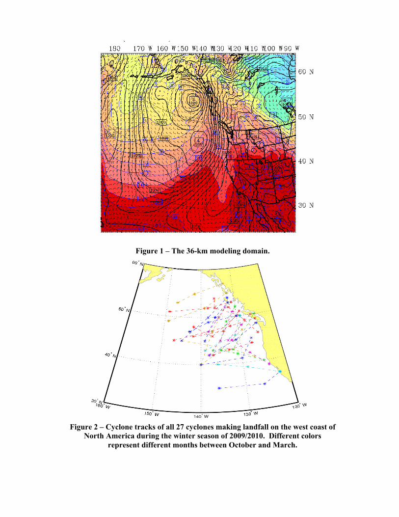
Figure 1 – The 36-km modeling domain.

Figure 2 – Cyclone tracks of all 27 cyclones making landfall on the west coast of North America during the winter season of 2009/2010. Different colors

represent different months between October and March.

NON-DEEPENING CYCLONE

Figure 3 – Analysis (left column) and 24-hr forecast (right column) of sea-level pressure (black contours, contour interval is 2hPa) and 925-hPa temperature (shaded) for a non-

deepening cyclone initialized at 1200 UTC October 16, 2009, a deepening cyclone initialized at 0000 UTC November 19, 2009, and a decaying cyclone initialized at 0600 UTC February

8, 2010. The blue arrows show the locations of the cyclones/cyclone precursors.

DEEPENING CYCLONE

DECAYING CYCLONE

DEEPENING CYCLONE

NON-DEEPENING CYCLONE

DECAYING CYCLONE Figure 4 – Ensemble sensitivity of the 24-hr average sea-level pressure response function

with respect to initial-time sea-level pressure (shaded, contour interval varies), and ensemble mean sea-level pressure (black contours, contour interval is 2 hPa) for the non-

deepening cyclone initialized at 1200 UTC October 16, 2009, the deepening cyclone initialized at 0000 UTC November 19, 2009, and the decaying cyclone initialized at 0600

UTC February 8, 2010. The green X symbols mark the location of the initial cyclone.

X

X

X

Figure 5 – Maximum magnitude of the ensemble sensitivity of the 24-hr average sea-level pressure response function with respect to initial-time sea-level pressure for all 27 cyclones

of the 2009/2010 winter season.

Figure 6 – Maximum magnitude of the ensemble sensitivity of the 24-hr average sea-level pressure response function with respect to initial-time geopotential height at 300, 500, 700,

850, and 925-hPa for all 27 cyclones of the 2009/2010 winter season.