Characterisation of the Neutron Field at the ANSTO...
58
Characterisation of the Neutron Field at the ANSTO Instrument Calibration Facility Haider Meriaty Quality, Safety, Environment, Radiation Protection, QSERP Australian Nuclear Science & Technology Organisation, ANSTO December 2009
Transcript of Characterisation of the Neutron Field at the ANSTO...
Characterisation of the Neutron Field
at the ANSTO Instrument Calibration
Facility
Haider Meriaty
Quality, Safety, Environment, Radiation Protection, QSERP
Australian Nuclear Science & Technology Organisation, ANSTO
December 2009

Characterisation of the Neutron Field at the ANSTO Instrument Calibration
Facility Published by the Australian Nuclear Science and Technology Organisation. © Commonwealth of Australia 2008 This work is copyright. Apart from any use as permitted under the Copyright Act 1968, no part may be reproduced by any process without prior written permission from the Commonwealth available from the Department of Communications, Information Technology and the Arts. Requests and enquiries concerning reproduction and rights should be addressed to the Commonwealth Copyright Administration, Intellectual Property Branch, Department of Communications, Information Technology and the Arts, GPO Box 2154, Canberra ACT 2601 or posted at http://www.dcita.gov.au/cca ISBN 1 921268 123 ANSTO Report No. ANSTO E-773 Front Cover Neutron Calibration Hall at ANSTO Instrument Calibration Facility
(ICF), December 2009 Photography Haider Meriaty, ANSTO
Contact Details ANSTO Australian Nuclear Science and Technology Organisation New Illawarra Road, Lucas Heights, NSW, Australia Postal Address Locked Bag 2001 Kirrawee DC, NSW 2234, Australia
Telephone + 61 2 9717 3111 Facsimile + 61 2 9543 5097 Email [email protected] Internet www.ansto.gov.au

ANSTO Report E-773 1
Table of Contents Abstract ...................................................................................................................................... 3
Keywords ................................................................................................................................... 3
INIS Descriptors......................................................................................................................... 3
1 Objectives........................................................................................................................... 4
2 Scope .................................................................................................................................. 4
3 Methods.............................................................................................................................. 4
3.1 Shadow Technique, ISO10647................................................................................... 4
3.2 Semi-Empirical Technique......................................................................................... 5
3.3 Polynomial Fitting Technique.................................................................................... 6
3.4 NCRP112 Technique.................................................................................................. 6
3.5 Shadow Cone Assembly............................................................................................. 6
3.6 Data Manipulation and Fitting ................................................................................... 7
3.7 Uncertainties............................................................................................................... 8
4 Materials............................................................................................................................. 8
4.1 Lithium Bromine (LiBr)............................................................................................. 8
4.1.1 Concentration-Adjustment Factor (CAF)........................................................... 8
4.2 Preparation of LiBr Solution ...................................................................................... 9
4.3 Trays and Cone Shell ............................................................................................... 10
4.4 Support Stand ........................................................................................................... 11
4.5 Iron Section of Shadow Cone................................................................................... 11
4.6 Neutron Source......................................................................................................... 12
5 Tools and Instrumentation................................................................................................ 13
5.1 Shadow Shield Assembly......................................................................................... 13
5.2 Materials’ Effects on Neutron Scatters and Absorptions ......................................... 14
5.2.1 Absorption of Thermal Neutrons ..................................................................... 14
5.2.2 Moderation of Fast Neutrons............................................................................ 15
5.3 Neutron Monitors ..................................................................................................... 16
5.4 Timer ........................................................................................................................ 17
5.5 Correction Factors & Parameters ............................................................................. 17
6 Calibration Room ............................................................................................................. 18
7 Setup and Acquisitions..................................................................................................... 20
7.1 Shadow Shield Assembly......................................................................................... 20
7.2 Neutron Monitor....................................................................................................... 20
7.3 Acquisitions.............................................................................................................. 20
8 Results and Analysis ........................................................................................................ 20
8.1 Free-Field Fluence and Dose Rate ........................................................................... 20
8.2 Dose Rate Measurements ......................................................................................... 22
8.3 Shadow Shield Method in ISO 10647 Standard....................................................... 24
8.3.1 Characteristic Constant, k ................................................................................ 24
8.3.2 Performance Test of LiBr Shadow Shield........................................................ 26
8.4 Semi-Empirical Method in ISO 10647 Standard ..................................................... 26
8.5 Polynomial Fit Method in ISO 10647 Standard....................................................... 29
8.5.1 Forsythe Orthogonal Fitting ............................................................................. 29
ANSTO Report E-773 2
8.5.2 Power Matrix Fitting ........................................................................................ 30
8.6 Shadow Method in NCRP5,4
112 Report.................................................................. 31
8.6.1 Fractional Dose Rate of Free Field Neutrons................................................... 31
8.6.2 Fractional Room Return Scatter ....................................................................... 32
8.7 Summary of Fractional Room Return Scatter and Monitor Response..................... 35
9 Discussion ........................................................................................................................ 36
10 Conclusions .................................................................................................................. 39
11 Appendices ................................................................................................................... 40
11.1 Advantages of Different Techniques........................................................................ 40
11.2 Limitations of Different Techniques ........................................................................ 40
11.3 Comparison of ICF Characterisation with PTB Calibration .................................... 41
11.4 PTB Calibration Certificate of ICF Reference Monitor........................................... 42
List of Tables............................................................................................................................ 49
List of Equations ...................................................................................................................... 51
List of Equations ...................................................................................................................... 51
List of Figures .......................................................................................................................... 52
References ................................................................................................................................ 53
ANSTO Report E-773 3
Abstract ANSTO’s Instrument Calibration Facility (ICF) provides calibration services to radiation
monitors, used in radiation protection applications. The facility has a large calibration room
that accommodates the neutron source rig and the monitor table, which is remotely controlled.
The room also hosts the gamma calibration services.
Determination of the free field (direct) and scattered components of neutron field in a
calibration room was essential to obtain an accurate response of the neutron monitor under
testing. The free field fluence response and the fractional room return scatter, caused by the
interaction of neutron fluence with the room structure, were determined. The fluence response
was 1.210x10⁻⁴
µSv/h per n/m2; and the neutron field has a fractional room scatter of 0.044 at
1 m and increases linearly versus square of distance.
The standard calibration methods, described by ISO-10647, IAEA-TR285, NCRP-112 and
NPL-RS(EXT)5, were utilized in this characterisation and gave comparable results.
The shadow-shield (truncated cone) were found more suitable to describe the neutron field
compared with the other methods e.g. the polynomial fitting, semi-empirical due to the fact of
the size, shape of the ICF room and source/monitor positions. Nevertheless; all methods
resulted in good response curves with correlation coefficients of fitting greater than 0.97.
The shadow shield consisted of two stacked conical sections. The first section was made from
iron of 200mm height and the second section was a hollow and made from aluminium of
350mm height. The hollow section was then filled with neutron-moderating/absorbing
materials i.e. water solution of LiBr 24% w/w. A performance test was conducted on the
shield and gave a very satisfactory result e.g. the readings of fluence response to the free field
neutron did follow the inverse square law with correlation >=0.999.
It is worth noticing that at the completion of this characterisation and report, the calibration
results with the Physikalische-Technische Bundesanstalt (PTB) in Germany became available.
As a result, the neutron characterisation at ICF calibration room did agree with the BTP
calibration within five percent. Consequently, the neutron field in ICF rig calibration room is
now traceable to BTP standard laboratory in Germany. Also, this agreement confirms the
integrity of the current neutron source e.g. anisotropy stability, which should save substantial
cost and efforts in replacing the source or sending it overseas for re-certification.
Keywords neutron ambient dose equivalent, neutron monitor calibration, neutron field characterisation,
monitor calibration with 241
Am/Be source, shadow shield calibration, neutron field
characterisation at ANSTO-ICF.
INIS Descriptors neutron monitors, BF3 counters, long counters, radiation monitoring, scattering. calibration
standards, interlaboratory comparisons.

ANSTO Report E-773 4
1 Objectives To determine the fractional room return scatter of a neutron field in the Instrument Calibration
Facility (ICF) calibration room.
To determine the dose equivalent response of the ICF reference neutron monitor
(Digipig2222).
2 Scope This calibration applied to dose equivalent neutron monitors of type Digipig, Elinor, Studsvik
or similar monitor using 241
Am/Be neutron source.
The front end of the monitor moderator shall face the neutron source. This arrangement is also
called End-On or 0o angle, in which the detector axis superimposes with the line of sight to
the centre of the neutron source.
Throughout this report, the terms ‘direct neutrons’, ‘cone’ and ‘distance’ will refer to the free
field neutrons, the shadow shield and effective distance (between source and monitor)
respectively. They may be used interchangeably.
3 Methods The shadow shield (a truncated-cone), the semi-empirical and the polynomial fitting methods
were applied to determine the ‘fractional room return scatter’ and the monitor response.
Details of these techniques are described in ISO standards1,2,3
(8529, 8529-3, 10647), IAEA
Technical Report Series4 285, NCRP Report
5 112 and other relevant papers
6,7,8,9,10,11. The
results of these techniques were then compared.
The advantages and limitations of each technique are given in the ISO 10647 standard3 and
are summarised in the appendix of this report.
3.1 Shadow Technique, ISO10647
This method uses a truncated cone filled with neutron absorber to shield the monitor from the
direct emission of a neutron source. The shield was placed halfway between the source and
monitor. Nine measurements (MS) were then taken between a range of 1 to 5 metres. At each
position, the measurement was repeated five times; the measurement was carried out using the
monitor’s integral mode over a period of five minutes. However at 1 metre, the cone was
placed closer to the source in order to provide a sufficient air gap at the monitor’s front and
optimise the deviation from the linear relation of air scatter required by the method. This
limited source / monitor distance of 1 metre and the relatively long cone of 0.55m left only
0.45m air-total gap to be utilised.
Similar measurements (MT) were repeated but without the shadow cone, which gave the total
monitor reading of direct and scattered components of the neutrons. Therefore, the reading
difference ∆M=MT–MS represents the net reading. This net should follow the inverse-square
law3 (ISL), providing it is corrected for all extraneous air scatter and geometry effects. The

ANSTO Report E-773 5
distance (l) in the ISL corresponds to the effective source-detector distance. The effective
detector centre is marked on the monitor’s moderator. ∆M is then given by the following
equation:
(1) ∆∆∆∆M . FA(llll) = k / llll 2
Where:
FA(l) is the corresponding air-attenuation factor (air-outscatter) as a function of
distance.
k is the source-detector Characteristic Constant i.e. monitor reading at unit
distance, fully corrected for all scattering effects.
k value is determined by first order linear fitted function. Thus, a plot of ∆M.FA(l) as a
function of (1/l 2) should illustrate a straight line with its slope equal to k value. The monitor
response is then obtained from the relationship3 between k, the fluence rate response (Rφ) and
the neutron angular source strength (BΩ).
(2) k = Rφφφφ . BΩ
The function in equation (1) should ideally have no intercept coefficient i.e. it passes through
the coordinate’s origin. Otherwise, any intercept value should be subtracted from the reading
when this equation is applied in the client’s routine calibration.
The fulfilment of measurement data with the ISL indicates a good integrity and functionality
of a shadow shield.
3.2 Semi-Empirical Technique
This technique assumes that the fraction of the monitor reading, caused by the scattered
neutrons, can be deduced from the reading’s deviation from the inverse-squared law. The
relationship between the monitor readings is considered as the sum of two components, which
is brought about by the direct and scattered neutron fluences. The relationship represents the
monitor’s fluence response as a function of distance and is given in equation (3) below.
(3) MT / [φφφφ . Fl(llll) . (1 + A . l l l l )] = RΦΦΦΦ (1 + S . l l l l 2)
Where:
A is the air scatter component. A=0.9% for 241
Am/Be source3.
S is the fractional room scatter contribution at unit test distance.
φ is the neutron fluence rate.
l is the effective source detector distance.
MT is the total reading i.e. both direct and scattered neutrons.
A plot of left-hand side (LHS) of equation (3) versus l 2 should yield a straight line. The
intercept of the line with the LHS axis represents the Rφ value. The S value then corresponds
to the line’s slope divided by Rφ .
This technique3 is usually suitable for a small room e.g. less than 2mx2mx2m in dimension.

ANSTO Report E-773 6
3.3 Polynomial Fitting Technique
This technique utilises the equation3 (4) below, which is derived from the semi-empirical
equation (3) by expansion and ignoring the third order term that is relatively too small.
(4) MT / [φφφφ . Fl(llll)] = RΦΦΦΦ (1 + x . llll + y . l l l l 2)
Equation (4) is useful in obtaining or verifying the fluence rate response (Rφ). The x and y
parameters should be regarded as fitting parameters i.e. no physical significance shall be
ascribed to them namely room scatter, S. These parameters incorporate the correction for the
total air scatter i.e. inscatter and outscatter.
Ten or more of data points are usually recommended3 for a good fit.
3.4 NCRP112 Technique
NCRP Report5 112 recommends equation (5) below to obtain the fractional room return
scatter factor (S).
(5) D. l l l l 2 = Do (1 + S. l l l l 2)
Where:
D is the monitor total reading, MT.
S is the line slope; it represents the scatter coefficient normalised at 1 metre.
Do is the deduced reading at 1 metre, from the source-neutrons exclusively.
In this approach, the total reading (MT) of dose rate should be corrected for the corresponding
air attenuation (FA) and geometry (F1) factors. The corrected values are then multiplied by the
square of the corresponding distances. The results are then plotted as a function of distance
squared (l 2).
The IAEA Report4 285 illustrates a similar approach and the derivation of the equation.
3.5 Shadow Cone Assembly
A truncated cone was constructed similar to the one described in the NCRP Report5 112.
However, the wax and Li2CO3 cone-section was replaced by a thin conical shell of aluminium
filled with aqueous LiBr solution of 24%w/w concentration - the solution served as a
moderator of fast neutrons as well as an absorber of the thermalised neutrons. This
concentration was equivalent to the 10% w/w Li2CO3 suggested in the NCRP Report 112.
A total scattering comparison between paraffin wax and water was performed to assess their
compatibility. Consequently, the scattering effects of the two moderators were found to be
compatible and satisfactory. The details are listed in the relevant tables provided in the Tools
and Instrumentation section.
A minimum mass of aluminium was used to construct the supporting table of the shadow
cone. Also, minimum hydrogenous or thermal neutron absorbent materials were kept in the
calibration room and at the same locations. These arrangements were intended to minimise
the scatter effects and ensure the consistency of ambient conditions in the calibration room.
ANSTO Report E-773 7
All measurements at a particular source-monitor distance were carried out over a fixed time
period of five minutes and repeated five times.
Two cross-hair laser beams were utilised to align the source, cone and neutron monitor with
an accuracy = < 1mm.
3.6 Data Manipulation and Fitting
Least Square Methods (LSM) were applied to fit data into polynomials function and
determine their coefficients12,13
. They included the Power and Orthogonal (Forsythe
approach) Polynomials14
.
The power polynomials required intensive matrix treatments in order to obtain the polynomial
coefficients. In addition, up to five measurement values could be fitted to avoid singularity of
coefficient matrix e.g. ISO standard3 recommends 10 data points for a good fit.
Alternatively, the Forsythe method accepts large number of fitting values and was later
applied, compared with LSM results and adopted.
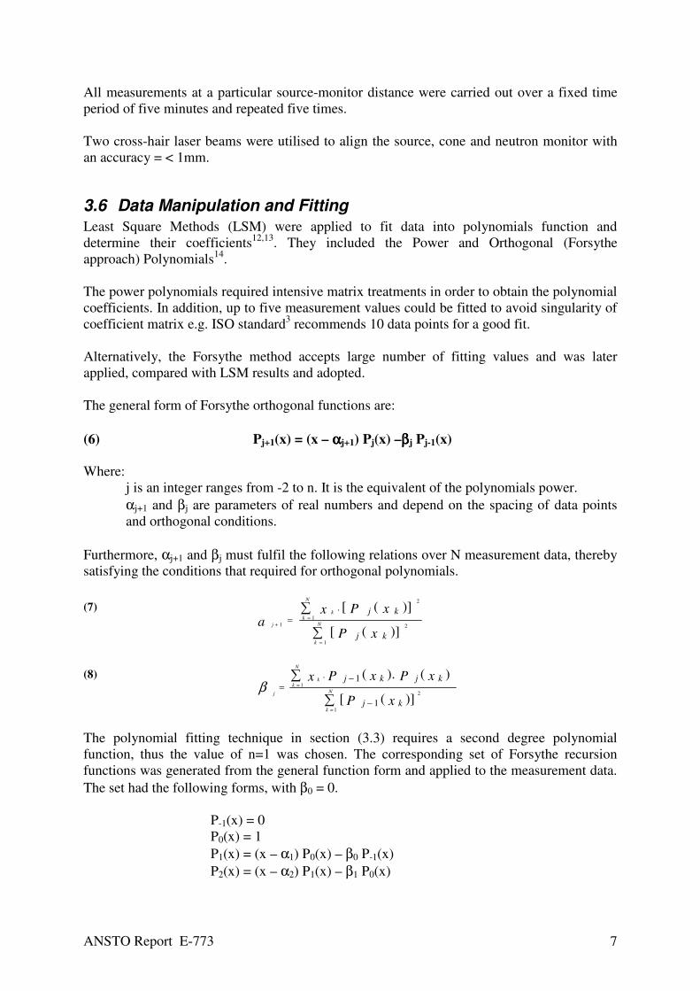
The general form of Forsythe orthogonal functions are:
(6) Pj+1(x) = (x – ααααj+1) Pj(x) –ββββj Pj-1(x)
Where:
j is an integer ranges from -2 to n. It is the equivalent of the polynomials power.
αj+1 and βj are parameters of real numbers and depend on the spacing of data points
and orthogonal conditions.
Furthermore, αj+1 and βj must fulfil the following relations over N measurement data, thereby
satisfying the conditions that required for orthogonal polynomials.
(7)
∑
∑
=
=+
=N
k
N
kk
j
xP
xPxa
kj
kj
1
2
1
2
1
)]([
)]([.
(8)
∑
∑
=
=
−
−=
N
k
N
kk
j
xP
xPxPx
kj
kjkj
1
2
1
)]([
)().(
1
1.
β
The polynomial fitting technique in section (3.3) requires a second degree polynomial
function, thus the value of n=1 was chosen. The corresponding set of Forsythe recursion
functions was generated from the general function form and applied to the measurement data.
The set had the following forms, with β0 = 0.
P-1(x) = 0
P0(x) = 1
P1(x) = (x – α1) P0(x) – β0 P-1(x)
P2(x) = (x – α2) P1(x) – β1 P0(x)

ANSTO Report E-773 8
The measurement data were applied to the following orthogonal polynomials and the
appropriated quadratic fit function was obtained:
(9) y = b0 . P0(x) + b1 . P1(x) + b2 . P2(x)
Where:
The polynomial coefficients bi were obtained from the following relationship:
(10)
∑
∑
=
==N
k
N
kk
i
xP
xPyb
ki
ki
1
2
1
)]([
)(.
Where:
i is 0,1 or 2.
k is the index of N measurement data.
yk and xk are the dependent and independent measurement datum respectively.
The above equations were programmed into an Excel Spreadsheet, Microsoft Office (97-
2003) and used to fit and evaluate the experiment data.
3.7 Uncertainties
Type ‘A’ combined uncertainties15,16,17
were applied to represent the statistical nature of
measurement’s errors.
Type ‘B’ uncertainties, given in ISO 10647 Standard3, are also relevant to this work. They
characterise the other uncertainties, which are caused by error sources that have a systematic
effect on that particular measurement.
4 Materials
4.1 Lithium Bromine (LiBr)
24%w/w of high purity LiBr powder was dissolved in de-ionised water (conductivity = 0.02
Mega Ohm-cm). The solution provides a moderating and absorbing medium to neutrons. This
concentration provided the equivalent 10%w/w concentration of Li2CO3, which suggested in
NCRP Report5 112. The calculation of the adjustment factor for LiBr is detailed in the next
section. This factor accounts for the molecular weight difference as well as the number of Li
atoms per molecule.
4.1.1 Concentration-Adjustment Factor (CAF)
Volume of Aluminium-cone shell = 7.1 L or 7100 cm3.
Water density = 1 g/cm3.
Thus water weight = 1x7100 = 7100 g or 7.1kg.
Weight of 10% w/w Li2CO3 = 7.1x10/100 = 0.71 kg.
Molecular weight18
of Li2CO3 = 74 g/mol.
Molecular weight18
of LiBr = 87 g/mol.

ANSTO Report E-773 9
Li is the absorber of thermal neutron. The ratio of Li abundance in the Li2CO3 and
LiBr compounds is 2. On the other hand, their molecular weight ratio is 74/87= 0.85.
Therefore,
CAF = 2/0.85 = 2.4.
The required weight of LiBr, which gives the same absorption effect as per Li2CO3, is
0.71xCAF = 0.71x2.4 = 1.7 kg.
Therefore,
w/w% LiBr is 1.7/7.1x100 = 24%.
4.2 Preparation of LiBr Solution
LiBr salt dissolves in water exothermically, thus care must be taken during the solution
preparation. As a guide, the following steps shall be applied for safe preparation and storage
of the solution. Always wear the appropriate protective gear during this preparation.
• Read the relevant chemical safety datasheets thoroughly e.g. MSDS.
• Place the solving container in a suitable heat-sink e.g. sink-basin and running water.
Fill the container to 50 percent of total solution volume.
• Add a small portion of the LiBr granulates (e.g. 10 percent of the total mass of the salt
at one time) into the container.
• Monitor the solution temperature and ensure that it stays below 60 oC.
• When all the salt is added, top up the solution to the required cone volume.
• Transfer the final solution, as soon as practical, into the cone-shell and secure its cap.
If the cone-shell is not internally coated with inert film e.g. wax or polyurethane, the solution
will react slowly with the shell wall and generate gas that will deform the cone shape as well
as cause the fracture/explosion of the shell. Therefore, the filled cone should not be
retained for more than one day. Alternatively, you MUST empty it and store it in a plastic
drum for future re-usage.
The LiBr solution must not be exposed to room air temperature for an extended time e.g. > 30
minutes. If it does it will absorb the ambient CO2 and form a Li2CO3 compound, which
precipitates and consequently affects the distribution uniformity and initial concentration of
the solution.
If the filled cone is not required for extended period of time e.g. months, transfer the solution
into an appropriate plastic container and secure its cap (i.e. air tight). Place the container into
a suitable drum (spill barrier) and store them in a safe and approved location.
The following specifications of Lithium Bromide (LiBr) granulates were applied to prepare
the cone-solution (see the table below).
Table 1: Specifications summary of the LiBr compound used in the solution preparation of a thermal
neutron absorber.
Formula LiBr
Formula Weight 86.85
Purity >=99%
Density 3.464
Brand Fluca, Cat.:62463
CAS code 7550-35-8
Lot S40883 32907B16

ANSTO Report E-773 10
Supplier Sigma-Aldrich, Sydney, Australia
Product of Germany
4.3 Trays and Cone Shell
A hollow truncated cone section (shell) and two trays were fabricated from aluminium sheets.
The sheet had the following industry identification: 1100 Alloy and O Temper as per ASME
SB209, which was supplied by Calm Aluminium PTY LTD.
The trays fitted onto the top of the stand and formed a supporting table. The shell mounted in
an aluminium cradle, made of the same sheet grade, and the combination was then positioned
on the supporting table during the measurements.
The maximum impurities (listed in Table 2), given in the material certificate as a weight
percentage, corresponded to a total impurity percentage of 0.63 percent. Rows six and nine in
the table give the weights of each individual impurity for the cone (Wshell) and trays (Wtrays)
respectively.
The total weight of the truncated-cone shell, including its cap was 628.8g.
The trays’ average size= 40x30cm and the total thickness was 2.4mm. Tray one and tray two
weigh 1080±20g and 1060±20g respectively (the total weight of both trays = 2140±20g). One
tray can fit into the other.
The macroscopic cross sections (whole target) of scatter (Σs) and absorption (Σa) of fabricated
aluminium materials and their impurities for the cone-shell and trays are listed in Table 2.
It was evident that the scatter and absorption effects caused by the impurities were relatively
much less than aluminium; and overall insignificant for the shell or trays.
Table 2: w/w% of impurities in aluminium sheets used in the fabrication of the cone shell and trays. The
macroscopic cross sections of these impurities are much less than the aluminium.
Al Si Fe Cu Mn Mg Cr Ni Zn Ti
A (g) 26.98 28.09 55.85 63.54 24.31 54.94 52 58.71 65.37 47.9
w/w% 99.37 0.09 0.4 0.07 0.03 0.007 0.001 0.006 0.005 0.02
σs (b) 1.5 2.17 11.62 8.03 2.15 3.71 3.49 18.5 4.13 4.35
σa (b) 0.23 0.17 2.56 3.78 13.3 0.06 3.05 4.49 1.11 6.09
Wshell (g) 624.84 0.57 2.52 0.44 0.19 0.04 0.01 0.04 0.03 0.13
ΣΣΣΣs (cm-1) 2.09E+01 2.63E-02 3.15E-01 3.35E-02 1.00E-02 1.79E-03 2.54E-04 7.16E-03 1.20E-03 6.88E-03
ΣΣΣΣa (cm-1) 3.21E+00 2.06E-03 6.94E-02 1.58E-02 6.21E-02 2.89E-05 2.22E-04 1.74E-03 3.21E-04 9.63E-03
Wtrays (g) 2126.54 1.93 8.56 1.50 0.64 0.15 0.02 0.13 0.11 0.43
ΣΣΣΣs (cm-1) 7.12E+01 8.96E-02 1.07E+00 1.14E-01 3.42E-02 6.09E-03 8.65E-04 2.44E-02 4.07E-03 2.34E-02
A : Atomic mass.
w/w% : weight to weight percentage of impurity.
σs : microscopic scatter cross section19 in barn (b) = 10-24 cm2.
σa : microscopic absorption cross section19 in barn (b) = 10-24 cm2.
Wshell : total weight of impurities in the shell.
Wtrays : total weight of impurities in the trays.
Σs : macroscopic cross sections of scatter (whole target).
Σa : macroscopic cross sections of absorption (whole target).

ANSTO Report E-773 11
4.4 Support Stand
An aluminium stand was fabricated and its top was designed and sized to fit the trays onto it
so as to form a supporting table. The assembly of cone and cradle was placed on the table top
during measurements (see Figure 2).
Hollow aluminium rods of a total mass = 3560g were used to fabricate the stand. The industry
specifications of the rods were as follows: Alloy: 60601 and Temper: T6, which was supplied
by Calm Aluminium, CA in the USA.
The following maximum impurities were listed in the material certificate as weight
percentage. This equated to 95.85 percent aluminium, hence the net mass of aluminium in the
rods was [(3560x95.9)/100] = 3412.26g.
The weight of the stand was 3560±20g. Thus, the weight difference accounted for the
auxiliary masses such as welding and screws at the stand’s legs. These additional masses were
considered insignificant, thus were not included in the cross section evaluation.
The macroscopic cross sections of scatter and absorption (whole stand) of aluminium and
their impurities are listed in Table 3.
It was evidence that the scatter and absorption effects caused by the impurities were relatively
much less than aluminium.
Table 3: w/w% of impurities in aluminium rods type which are used in fabrication of the support stand.
The macroscopic cross sections of these impurities are much less than the aluminium.
Al Si Fe Cu Mn Mg Cr Zn Ti Others
A (g) 26.98 28.09 55.85 63.54 24.31 54.94 52 65.37 47.9
w/w% 95.85 0.8 0.7 0.4 0.15 1.2 0.35 0.25 0.15 0.15
σs (b) 1.5 2.17 11.62 8.03 2.15 3.71 3.49 4.13 4.35
σa (b) 0.23 0.17 2.56 3.78 13.3 0.06 3.05 1.11 6.09
Wframe (g) 3412.26 28.48 24.92 14.24 5.34 42.72 12.46 8.90 5.34 5.34
ΣΣΣΣs (cm-1) 1.14E+02 1.32E+00 3.12E+00 1.08E+00 2.84E-01 1.74E+00 5.03E-01 3.38E-01 2.92E-01
ΣΣΣΣa (cm-1) 1.75E+01 1.04E-01 6.88E-01 5.10E-01 1.76E+00 2.81E-02 4.40E-01 9.10E-02 4.09E-01
A (g) : Atomic mass.
w/w% : weight to weight percentage of impurity.
σs : microscopic scatter cross section19 in barn (b) = 10-24 cm2.
σa : microscopic absorption cross section19 in barn (b) = 10-24 cm2.
Wframe : total weight of impurities in the aluminium frame.
Σs : Macroscopic cross section of whole target.
Σa : Macroscopic cross section of whole target.
4.5 Iron Section of Shadow Cone
The top part of the shadow cone was made of a solid iron section3,5
. This section was
fabricated from iron ingot of grade Flocast MF2. The maximum chemical compositions, given
by the material Analysis Certificate, are listed as weight percentage in Table 4, row three. The
volume of this section was 568cm3 and would weigh 4.47kg (using Fe density value
18 =
7.86g/cm3). The corresponding weights of the impurities in the section are listed in row six.
The macroscopic cross sections of scatter and absorption (whole section) of iron cone and
their impurities are listed in Table 4.
ANSTO Report E-773 12
It was evident that the scatter and absorption effects caused by the impurities were relatively
much less than iron.
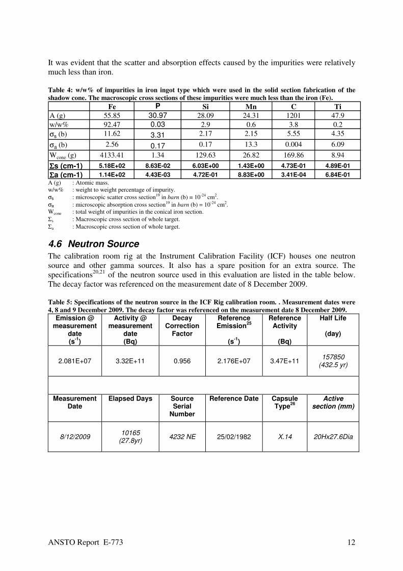
Table 4: w/w% of impurities in iron ingot type which were used in the solid section fabrication of the
shadow cone. The macroscopic cross sections of these impurities were much less than the iron (Fe).
Fe P Si Mn C Ti
A (g) 55.85 30.97 28.09 24.31 1201 47.9
w/w% 92.47 0.03 2.9 0.6 3.8 0.2
σs (b) 11.62 3.31 2.17 2.15 5.55 4.35
σa (b) 2.56 0.17 0.17 13.3 0.004 6.09
Wcone (g) 4133.41 1.34 129.63 26.82 169.86 8.94
ΣΣΣΣs (cm-1) 5.18E+02 8.63E-02 6.03E+00 1.43E+00 4.73E-01 4.89E-01
ΣΣΣΣa (cm-1) 1.14E+02 4.43E-03 4.72E-01 8.83E+00 3.41E-04 6.84E-01
A (g) : Atomic mass.
w/w% : weight to weight percentage of impurity.
σs : microscopic scatter cross section19 in barn (b) = 10-24 cm2.
σa : microscopic absorption cross section19 in barn (b) = 10-24 cm2.
Wcone : total weight of impurities in the conical iron section.
Σs : Macroscopic cross section of whole target.
Σa : Macroscopic cross section of whole target.
4.6 Neutron Source
The calibration room rig at the Instrument Calibration Facility (ICF) houses one neutron
source and other gamma sources. It also has a spare position for an extra source. The
specifications20,21
of the neutron source used in this evaluation are listed in the table below.
The decay factor was referenced on the measurement date of 8 December 2009.
Table 5: Specifications of the neutron source in the ICF Rig calibration room. . Measurement dates were
4, 8 and 9 December 2009. The decay factor was referenced on the measurement date 8 December 2009.
Emission @ measurement
date (s
-1)
Activity @ measurement
date (Bq)
Decay Correction
Factor
Reference Emission
25
(s
-1)
Reference Activity
(Bq)
Half Life
(day)
2.081E+07 3.32E+11 0.956 2.176E+07 3.47E+11 157850
(432.5 yr)
Measurement Date
Elapsed Days Source Serial
Number
Reference Date Capsule Type
26
Active section (mm)
8/12/2009 10165
(27.8yr) 4232 NE 25/02/1982 X.14 20Hx27.6Dia

ANSTO Report E-773 13
5 Tools and Instrumentation
5.1 Shadow Shield Assembly
This assembly consisted of two conical sections and an aluminium cradle. The conical
sections were horizontally fitted onto the cradle and formed one truncated cone. The cradle
was equipped with vertical plates to support each conical section as well as aligning their
axes.
The slant of the cone’s side was at an angle of 10.3o degrees to its central axis. The following
linear equation was derived to describe the cone-slanted side, thus to match the required
physical size for shadow technique5 setup (see Figure 1). This equation was used later to
calculate the volume (v) of the conical sections.
(11) y = 0.1818 x + 1
Where:
‘y’ represents the cone’s radius at height ‘x’.
The cone volume was calculated using the three dimensional integration method13
of
revolving function. Hence, the conical volume was generated when the linear function ‘y’ in
equation (12) revolved around the coordinate axis ‘x’ and integrated between the desired
height limits. The intercept value with the ‘oy’ axis corresponded to the radius of the smaller
cross section of truncated cone (i.e. radius = 1cm). Therefore, the conical volume (v) was
obtained by applying the following equation.
(12) v = π π π π ∫ (0.1818 x + 1) . dx
This equation was programmed into Mathematica22
software package (version 5) and
integrated to obtain the volumes and masses of conical sections.
Figure 1: Diagram of shadow cone and its sections. The narrow side faced the neutron source and the
wider one faced the monitor.
The features and specifications of the shadow cone assembly (cone block and cradle) were
listed in Table 6. The cone shell was filled with the LiBr solution.
Diameter
20mm Solid Iron
Diameter
220mm
LiBr Solution
24%w/w
200mm 350mm
ANSTO Report E-773 14
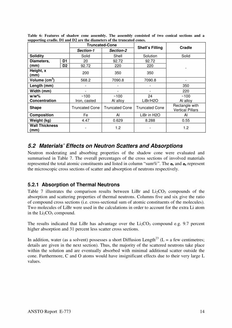
Table 6: Features of shadow cone assembly. The assembly consisted of two conical sections and a
supporting cradle. D1 and D2 are the diameters of the truncated cones.
Truncated-Cone
Section-1 Section-2 Shell’s Filling Cradle
Solidity Solid Shell Solution Solid
D1 20 92.72 92.72 Diameters, (mm) D2 92.72 220 220
Height, x (mm)
200 350 350
-
Volume (cm3) 568.2 7090.8 7090.8 -
Length (mm) - - - 350
Width (mm) - - - 220
w/w% Concentration
~100 Iron, casted
~100 Al alloy
24 LiBr/H2O
~100 Al alloy
Shape Truncated Cone Truncated Cone Truncated Cone Rectangle with Vertical Pillars
Composition Fe Al LiBr in H2O Al
Weight (kg) 4.47 0.629 8.288 0.55
Wall Thickness (mm)
- 1.2 - 1.2
5.2 Materials’ Effects on Neutron Scatters and Absorptions
Neutron moderating and absorbing properties of the shadow cone were evaluated and
summarised in Table 7. The overall percentages of the cross sections of involved materials
represented the total atomic constituents and listed in column “sum%”. The σσσσs and σσσσa represent
the microscopic cross sections of scatter and absorption of neutrons respectively.
5.2.1 Absorption of Thermal Neutrons
Table 7 illustrates the comparison results between LiBr and Li2CO3 compounds of the
absorption and scattering properties of thermal neutrons. Columns five and six give the ratio
of compound cross sections (i.e. cross-sectional sum of atomic constituents of the molecules).
Two molecules of LiBr were used in the calculations in order to account for the extra Li atom
in the Li2CO3 compound.
The results indicated that LiBr has advantage over the Li2CO3 compound e.g. 9.7 percent
higher absorption and 31 percent less scatter cross sections.
In addition, water (as a solvent) possesses a short Diffusion Length23
(L = a few centimetres;
details are given in the next section). Thus, the majority of the scattered neutrons take place
within the solution and are eventually absorbed with minimal additional scatter outside the
cone. Furthermore, C and O atoms would have insignificant effects due to their very large L
values.

ANSTO Report E-773 15
Table 7: Comparison results of the neutron cross sections of two compounds used as absorbers of thermal
neutron for shadow cone. The LiBr compound has an advantage over Li2CO3 in terms of less scatter and
more absorption of neutrons.
ElementAbandance
Fraction σσσσs σσσσa σσσσs σσσσa Element
Abandance
fraction σσσσs σσσσa
Li-6 0.0759 0.97 940 Li-6 0.0759 0.97 940
Li-7 0.9241 1.4 0.045 Li-7 0.9241 1.4 0.045
C 1 5.56 0.004 Br-79 0.5069 5.96 11
nil 0 0 0 Br-81 0.4931 5.84 2.7O 1 4.23 0.0001
Li2CO3 (b) 20.98 142.78 0.69 109.67 2LiBr (b) 14.54 156.59
Neutron Cross Section of Li2CO3 (b) Sum% Neutron Cross Section of 2LiBr (b)
(b): barn = 10
-24 cm
2.
5.2.2 Moderation of Fast Neutrons
The moderating properties of paraffin wax and water were evaluated and compared. The
results demonstrated comparable Diffusion Lengths23
(L) e.g. in order of a few centimetres
for hydrogen. L value incorporates the competing effects of the two types of cross sections,
e.g. absorption and scattering (see Table 8). The terminologies and their meanings, given in
the table, are explained in the following paragraphs.
Table 8: Comparison results of thermalised neutron properties of two compounds that were considered in
shadow shield construction.
Paraffin Wax Water
Molecular Formula24
C25H52 H2O
Hydrogen Ratio 2.08 2
Molecular Weight (g/mol)
352 18
Molecular Density (mol/cm
3)
1.59E+21 3.34E+22
H C H O Atomic Density (Atoms/cm
3)
8.27E22 3.98E+22 6.69E+22 3.34E+22
σσσσa 0.33 0.004 0.33 0.0001 Microscopic Cross Sections
(b) σσσσs 82.03 5.56 82.03 4.23
Σa 2.73E-02 1.59E-04 2.21E-02 3.34E-06 Macroscopic Cross Sections
(cm-1
) Σs 6.78E+00 2.21E-01 5.49E+00 1.41E-01
λλλλa 3.66E+01 6.29E+03 4.53E+01 2.99E+05
λλλλs 1.47E-01 4.52E+00 1.82E-01 7.07E+00 Mean Free Path
(cm) λλλλtr 0.69 2931.81 0.85 8144.25
Average Cosine of Deflected Angle (Lab-
System)
µµµµ 0.786 0.998 0.786 0.999
Diffusion Length (cm)
L 2.90 2479.3 3.59 28490.5
ANSTO Report E-773 16
(b): barn = 10-24
cm2.
The molecular density represents the actual number of molecules per cubic centimetre of a
compound.
The atomic density is equal to the molecular density times the number of atoms. It was then
applied to calculate the corresponding macroscopic cross sections of an intended compound.
The Mean Free Path23
(λa/s) of absorption or scattering represents the total path that a neutron
traces before absorbed or scattered by the medium. It is given as λa/s = 1/N.σa/s where N is the
number of nuclei per cubic centimetre in a medium.
The Transport Mean Free Path is a function of λs and the Scattering Angle (θ). It is given as
λtr = λs/[1-cos(θ)].
The Diffusion Length constant23
(L) represents the average distance (line of sight) that a
neutron moves from its initial plane before absorption. It concurrently combines λa and λtr
effects and is defined by the following relationship: L = [(λa .λt)/3]1/2
.
Consequently, the Paraffin or water media exhibited comparable effects on the neutron
slowing down range as illustrated by the calculated L values of hydrogen.
5.3 Neutron Monitors
The ICF reference neutron monitor was used throughout the characterisation measurements of
the rig calibration room. The monitor had an ANSTO tag indicating an in situ check of
reading consistency, valid up to 10 March 2010. It was manufactured by Wedholm Medical in
Sweden (www.wedholmmedical.se). However, the monitor had no documentation of
traceability to standard calibration authority. A traceable calibration was then sought to be
initiated once this characterization completed, thus avoiding any delay to the work.
Furthermore, the calibration factor provided by the authority will then be applied to the final
characterisation outcomes prior to commissioning of the calibration room for routine neutron
services to clients.
The monitor calibration typically takes four to six months by an external recognisable
standard laboratory.
The manual25
of the ICF monitor includes a Test Certificate no Kp-06067 dated 17 December
2007. The monitor’s certificate reported a neutron sensitivity of 0.40 cps/microSv/h and a
good linearity.
The Digipig monitor (2222A) employed a BF3 detector, polyethylene moderator, borated
plastic absorber and digital display. The monitor’s energy response was in close agreement
with an ICRP74 neutron sensitivity response curve.
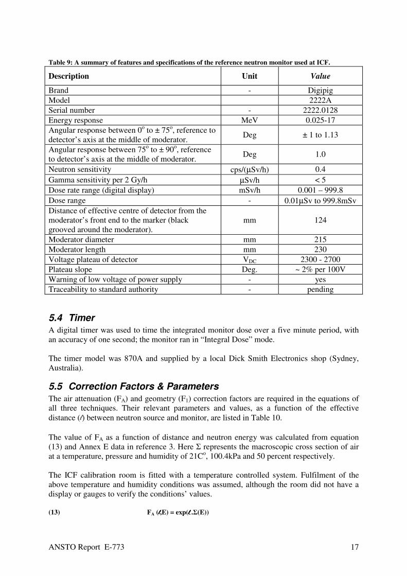
The monitor has several measurement modes such as dose rate and accumulated dose
(updated at 100 seconds interval). A summary of the ICF monitor’s specifications are listed in
the table below.
ANSTO Report E-773 17
Table 9: A summary of features and specifications of the reference neutron monitor used at ICF.
Description Unit Value
Brand - Digipig
Model 2222A
Serial number - 2222.0128
Energy response MeV 0.025-17
Angular response between 0o to ± 75
o, reference to
detector’s axis at the middle of moderator. Deg ± 1 to 1.13
Angular response between 75o to ± 90
o, reference
to detector’s axis at the middle of moderator. Deg 1.0
Neutron sensitivity cps/(µSv/h) 0.4
Gamma sensitivity per 2 Gy/h µSv/h < 5
Dose rate range (digital display) mSv/h 0.001 – 999.8
Dose range - 0.01µSv to 999.8mSv
Distance of effective centre of detector from the
moderator’s front end to the marker (black
grooved around the moderator).
mm 124
Moderator diameter mm 215
Moderator length mm 230
Voltage plateau of detector VDC 2300 - 2700
Plateau slope Deg. ~ 2% per 100V
Warning of low voltage of power supply - yes
Traceability to standard authority - pending
5.4 Timer
A digital timer was used to time the integrated monitor dose over a five minute period, with
an accuracy of one second; the monitor ran in “Integral Dose” mode.
The timer model was 870A and supplied by a local Dick Smith Electronics shop (Sydney,
Australia).
5.5 Correction Factors & Parameters
The air attenuation (FA) and geometry (F1) correction factors are required in the equations of
all three techniques. Their relevant parameters and values, as a function of the effective
distance (l) between neutron source and monitor, are listed in Table 10.
The value of FA as a function of distance and neutron energy was calculated from equation
(13) and Annex E data in reference 3. Here Σ represents the macroscopic cross section of air
at a temperature, pressure and humidity of 21Co, 100.4kPa and 50 percent respectively.
The ICF calibration room is fitted with a temperature controlled system. Fulfilment of the
above temperature and humidity conditions was assumed, although the room did not have a
display or gauges to verify the conditions’ values.
(13) FA (llll,E) = exp(llll.....Σ(E))

ANSTO Report E-773 18
The value of F1 was calculated from the following equation3, in which ‘r’ represents the
radius of sphere or cylinder.
(14) F1(llll) = 1 + δ . (r/2 . llll)2
The values of Σ and δ, used in the equations of the correction factors, were taken from the
ISO 10647 standard3 for
241Am/Be source. Also, the value of total air scatter (A) used in the
semi-empirical equation was taken from the same reference.
Values of FA and Fl related to the monitor and calibration room of ICF are listed in Table 10.
Table 10: A list of air attenuation (FA), geometry (F1) and correction factors as a function of the effective
distance (llll) between neutron sources and the monitor. Also, parameters used in the calculations are also
listed:
Effective Distance, llll
(m)
LLLL 2
(m2)
F1(llll) δ (effectiveness
parameter)
Air-Scatter parameter,
A
Air-Attenuation Correction,
FA(l)
Σ Σ Σ Σ
((((m−1−1−1−1))))
0.12 0.0144 1.1003 1.0011
0.25 0.0625 1.0231 1.0022
0.5 0.25 1.0058 1.0045
1 1 1.0014 0.5 0.009 1.0089 0.0089
1.5 2.25 1.0006 1.0134
2 4 1.0004 1.0180
2.5 6.25 1.0002 1.0225
3 9 1.0002 1.0271
3.5 12.25 1.0001 1.0316
4 16 1.0001 1.0362
4.5 20.25 1.0001 1.0409
5 25 1.0001 1.0455
6 Calibration Room The ICF calibration room has a solid concrete floor and is surrounded by double walls with a
total thickness of about 600mm. The walls are built from solid concrete blocks. The internal
faces of the walls are lined with gypsum panels of 20mm thickness. The height of these
panels is about 75 percent of the wall’s height.
The dimensions of the room are shown on the engineering plan (see Figure 2). The guide tube
of the source is positioned at the centre of the room’s widest section. The radius between the
source-guide to the closest wall is 3.4 metres.
The room’s roof is made of metal alloy (e.g. collar-bond) and positioned at a height =
9300mm. A standard “false” ceiling is also installed in the room at a height = 6000mm.
The rig system is equipped with an aluminium calibration table of adjustable height. The table
movement along the rail-guide is computer-driven (from the control room) and has a range of
200mm to 5000mm from the source. The accuracy of table displacement is less than 2mm.
The rail is bolted to the room’s floor and oriented diagonally to minimise the wall’s scatter.
ANSTO Report E-773 19
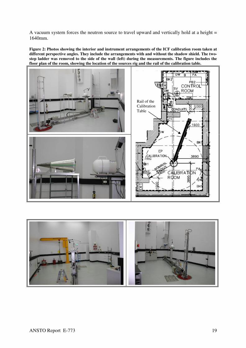
A vacuum system forces the neutron source to travel upward and vertically hold at a height =
1640mm.
Figure 2: Photos showing the interior and instrument arrangements of the ICF calibration room taken at
different perspective angles. They include the arrangements with and without the shadow shield. The two-
step ladder was removed to the side of the wall (left) during the measurements. The figure includes the
floor plan of the room, showing the location of the sources rig and the rail of the calibration table.
Rail of the
Calibration
Table

ANSTO Report E-773 20
7 Setup and Acquisitions
7.1 Shadow Shield Assembly
The support table was positioned half way between the neutron source and rail-calibration
stand. The shadow shield assembly was then placed on the support table, where the narrow
cone’s end faced the source (Fig 2).
The monitor was placed on the rail-stand and its effective centre mark aligned with the rail’s
distance marker. The stand was positioned at the desired distance from the control room. The
monitor’s front face (the moderator’s base) was pointed toward the source (0o angle between
the line of sight and the moderator’s axis).
The combination of the mid-source was sagittally and laterally aligned with the axes of
shadow shield as well as the monitor’s moderator, using the cross hair of two laser units and
reference markers on the walls of the ICF rig-room. The accuracy of the alignment was <
1mm.
The monitor reading was viewed via the CCT camera / monitor system from the control room
and recorded by the operator.
7.2 Neutron Monitor
The ‘Integral’ mode of monitor reading was applied over a period of five minutes. A digital
timer was used to keep track of the measurement period.
The operator used a two-step aluminium ladder to reach the monitor display and the CCTV
camera. The operator activated the timer and monitor’s acquisition concurrently, descended to
the room floor and moved the ladder next to the tool bench and then left the room quickly.
7.3 Acquisitions
Measurements were taken at nine positions, covering a range from 1 metre to 5 metres at an
interval of 0.5m. At each interval, five accumulative readings were recorded at five minute
intervals. The net monitor reading at each time segment was then calculated by taking the
difference between the current and last reading. The source transit time was avoided by taking
an extra reading initially.
Every session of measurement was proceeded by a background measurement of the ICF room
over a period of 15 minutes (at least) and found to be zero. Also, the battery status was
checked and replaced if required. The solution level in the cone shell was also checked prior
to and after each measurements session. No additional filling was required throughout the
measurements.
8 Results and Analysis
8.1 Free-Field Fluence and Dose Rate
The reference neutron fluence, given in the NPL Calibration Certificate20
, was corrected for
decay to the measurement date (8 December 2009) and then applied to calculate the expected
ANSTO Report E-773 21
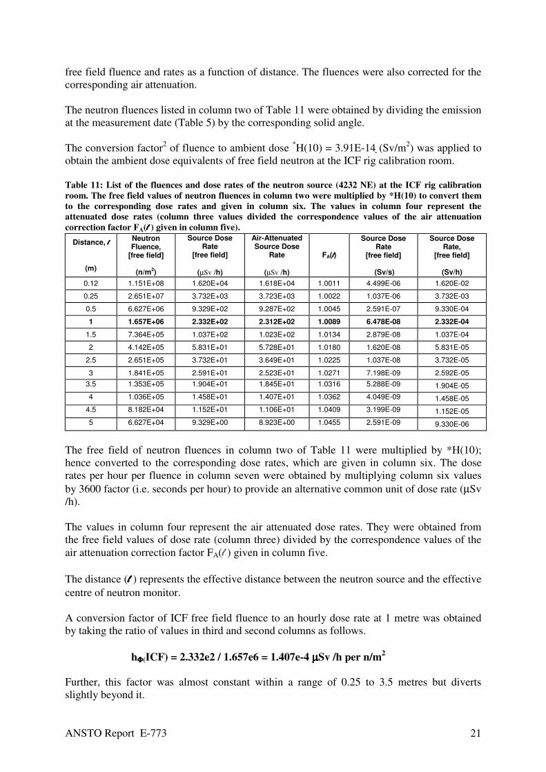
free field fluence and rates as a function of distance. The fluences were also corrected for the
corresponding air attenuation.
The neutron fluences listed in column two of Table 11 were obtained by dividing the emission
at the measurement date (Table 5) by the corresponding solid angle.
The conversion factor2 of fluence to ambient dose
*H(10) = 3.91E-14 (Sv/m
2) was applied to
obtain the ambient dose equivalents of free field neutron at the ICF rig calibration room.
Table 11: List of the fluences and dose rates of the neutron source (4232 NE) at the ICF rig calibration
room. The free field values of neutron fluences in column two were multiplied by *H(10) to convert them
to the corresponding dose rates and given in column six. The values in column four represent the
attenuated dose rates (column three values divided the correspondence values of the air attenuation
correction factor FA(l l l l ) given in column five).
Distance, llll
(m)
Neutron Fluence,
[free field]
(n/m2)
Source Dose Rate
[free field]
(µSv /h)
Air-Attenuated Source Dose
Rate
(µSv /h)
FA(llll)
Source Dose Rate
[free field]
(Sv/s)
Source Dose Rate,
[free field]
(Sv/h)
0.12 1.151E+08 1.620E+04 1.618E+04 1.0011 4.499E-06 1.620E-02
0.25 2.651E+07 3.732E+03 3.723E+03 1.0022 1.037E-06 3.732E-03
0.5 6.627E+06 9.329E+02 9.287E+02 1.0045 2.591E-07 9.330E-04
1 1.657E+06 2.332E+02 2.312E+02 1.0089 6.478E-08 2.332E-04
1.5 7.364E+05 1.037E+02 1.023E+02 1.0134 2.879E-08 1.037E-04
2 4.142E+05 5.831E+01 5.728E+01 1.0180 1.620E-08 5.831E-05
2.5 2.651E+05 3.732E+01 3.649E+01 1.0225 1.037E-08 3.732E-05
3 1.841E+05 2.591E+01 2.523E+01 1.0271 7.198E-09 2.592E-05
3.5 1.353E+05 1.904E+01 1.845E+01 1.0316 5.288E-09 1.904E-05
4 1.036E+05 1.458E+01 1.407E+01 1.0362 4.049E-09 1.458E-05
4.5 8.182E+04 1.152E+01 1.106E+01 1.0409 3.199E-09 1.152E-05
5 6.627E+04 9.329E+00 8.923E+00 1.0455 2.591E-09 9.330E-06
The free field of neutron fluences in column two of Table 11 were multiplied by *H(10);
hence converted to the corresponding dose rates, which are given in column six. The dose
rates per hour per fluence in column seven were obtained by multiplying column six values
by 3600 factor (i.e. seconds per hour) to provide an alternative common unit of dose rate (µSv
/h).
The values in column four represent the air attenuated dose rates. They were obtained from
the free field values of dose rate (column three) divided by the correspondence values of the
air attenuation correction factor FA(l ) given in column five.
The distance (llll ) represents the effective distance between the neutron source and the effective
centre of neutron monitor.
A conversion factor of ICF free field fluence to an hourly dose rate at 1 metre was obtained
by taking the ratio of values in third and second columns as follows.
hΦΦΦΦ(ICF) = 2.332e2 / 1.657e6 = 1.407e-4 µµµµSv /h per n/m2
Further, this factor was almost constant within a range of 0.25 to 3.5 metres but diverts
slightly beyond it.

ANSTO Report E-773 22
8.2 Dose Rate Measurements
The monitor readings at the desired distances, with and without the shadow cone, are listed in
Table 12. The distance ‘l ‘ represents the direct distance between the source-central axis and
the effective-centre of the monitor. The effective centre was marked by a black groove around
the moderator. The effective centre was 124mm away from the front face of the moderator.
The total and shadow measurements were obtained in two separate sessions. The Total Dose
Rate, MT represents the reading of the free field and scattered components of the incident
neutrons on the monitor.
The Shadow Dose Rate, Ms represents the scatter reading while the shadow shield was
positioned at the middle distance between the source and monitor blocking the direct
neutrons.
Measurements at 1 metre were performed with the shadow cone placed closer to the source
rather than at an equidistance, in contrast with the rest of measurements. However, this
arrangement was necessary to allow a sufficient air gap between the cone face and the
monitor, so optimising the linear relation3,4,11
between air inscatter and net scatters (i.e.
inscatter minus outscatter). The recommended ratio3,4
of gap to cone length is of order of one
or more in order to obtain a linear net scatter with uncertainty < three percent.
The distance between the cone’s small face and source was set at 50mm. This arrangement
provided a gap of 400mm, which corresponded to 73 percent of the recommended ratio3,5
.
Details of the calculation are as follows.
Source to monitor distance = 1000mm
Shadow cone length = 550mm
Source to cone’s front face (small) = 50mm
Monitor to cone’s rear face (large) = 1000 - (550 + 50) = 400mm
Ratio = 400 / 550 = 0.73
Table 12: List of the initial reading values by the ICF monitor with and without the shadow shield. The
Total Dose Rate corresponded to the direct and scattered neutrons detected by the monitor. The shadow
Dose Rate corresponds to the scattered neutrons only.
Distance, llll
(mm)
Total Dose Rate, MT
(µµµµSv/5min)
Shadow Dose Rate, Ms
(µµµµSv/5min)
1000 19.114 2.6
1000 19.11 2.618
1000 19.48 2.643
1000 19.11 2.61
1000 19.25 2.63
1500 9.399 2.189
1500 9.244 2.177
1500 9.37 2.19
1500 9.41 2.204
1500 9.09 2.2
2000 5.708 1.815
2000 5.649 1.821
2000 5.74 1.784

ANSTO Report E-773 23
The readings of initial measurements were averaged at each distance and listed in Table 13
with their associated statistical sample standard deviations. These values were then utilised to
obtain the relevant characterisation parameters of the neutron field and rig-calibration room.
Table 13: List of the average dose rate readings of total and shadow configurations obtained by the ICF
neutron monitor. Their associated sample standard deviations (SD) were also listed. Distance, llll
(mm)
Total Reading, MT
(µµµµSv/5min)
SD-Total
(µµµµSv/5min) %SD-Total
Shadow Reading, MS
(µµµµSv/5min)
SD-Shadow
(µµµµSv/5min) %SD-Shadow
1000 19.213 0.161 0.8 2.620 0.017 0.6
1500 9.303 0.136 1.5 2.192 0.011 0.5
2000 5.715 0.049 0.9 1.800 0.025 1.4
2500 4.104 0.055 1.3 1.581 0.035 2.2
3000 3.169 0.045 1.4 1.422 0.009 0.6
3500 2.560 0.032 1.3 1.244 0.027 2.1
4000 2.092 0.054 2.6 1.148 0.033 2.8
4500 1.786 0.038 2.1 1.023 0.033 3.2
5000 1.546 0.020 1.3 0.926 0.035 3.8
2000 5.7 1.814
2000 5.78 1.764
2500 4.041 1.604
2500 4.163 1.525
2500 4.086 1.585
2500 4.16 1.614
2500 4.07 1.575
3000 3.109 1.417
3000 3.226 1.415
3000 3.153 1.437
3000 3.197 1.424
3000 3.16 1.417
3500 2.532 1.204
3500 2.593 1.253
3500 2.572 1.248
3500 2.582 1.277
3500 2.52 1.239
4000 2.077 1.172
4000 2.077 1.13
4000 2.118 1.105
4000 2.168 1.187
4000 2.022 1.145
4500 1.749 1.043
4500 1.765 1.051
4500 1.783 0.969
4500 1.785 1.018
4500 1.848 1.035
5000 1.531 0.882
5000 1.568 0.899
5000 1.567 0.934
5000 1.528 0.951
5000 1.535 0.965
ANSTO Report E-773 24
8.3 Shadow Shield Method in ISO 10647 Standard
8.3.1 Characteristic Constant, k
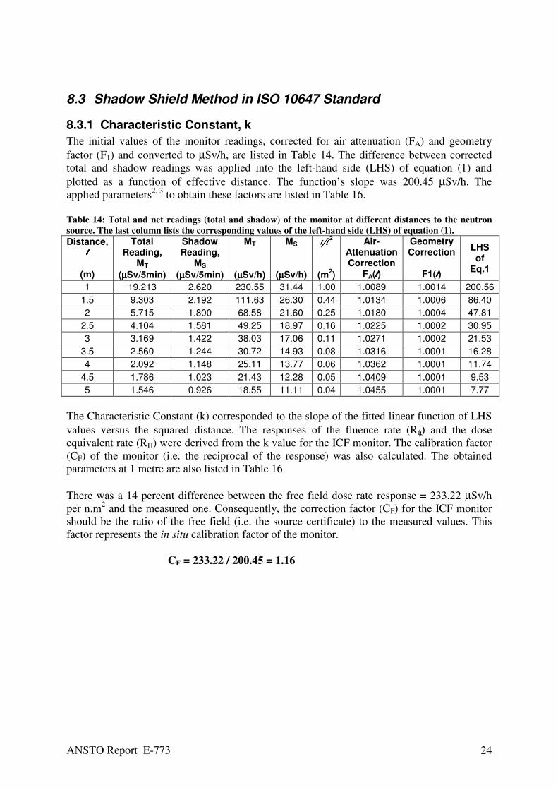
The initial values of the monitor readings, corrected for air attenuation (FA) and geometry
factor (F1) and converted to µSv/h, are listed in Table 14. The difference between corrected
total and shadow readings was applied into the left-hand side (LHS) of equation (1) and
plotted as a function of effective distance. The function’s slope was 200.45 µSv/h. The
applied parameters2, 3
to obtain these factors are listed in Table 16.
Table 14: Total and net readings (total and shadow) of the monitor at different distances to the neutron
source. The last column lists the corresponding values of the left-hand side (LHS) of equation (1).
Distance, llll
(m)
Total Reading,
MT
(µµµµSv/5min)
Shadow Reading,
MS
(µµµµSv/5min)
MT
(µµµµSv/h)
MS
(µµµµSv/h)
1/1/1/1/LLLL2
(m2)
Air-Attenuation Correction
FA(llll)
Geometry Correction
F1(llll)
LHS of
Eq.1
1 19.213 2.620 230.55 31.44 1.00 1.0089 1.0014 200.56
1.5 9.303 2.192 111.63 26.30 0.44 1.0134 1.0006 86.40
2 5.715 1.800 68.58 21.60 0.25 1.0180 1.0004 47.81
2.5 4.104 1.581 49.25 18.97 0.16 1.0225 1.0002 30.95
3 3.169 1.422 38.03 17.06 0.11 1.0271 1.0002 21.53
3.5 2.560 1.244 30.72 14.93 0.08 1.0316 1.0001 16.28
4 2.092 1.148 25.11 13.77 0.06 1.0362 1.0001 11.74
4.5 1.786 1.023 21.43 12.28 0.05 1.0409 1.0001 9.53
5 1.546 0.926 18.55 11.11 0.04 1.0455 1.0001 7.77
The Characteristic Constant (k) corresponded to the slope of the fitted linear function of LHS
values versus the squared distance. The responses of the fluence rate (Rφ) and the dose
equivalent rate (RH) were derived from the k value for the ICF monitor. The calibration factor
(CF) of the monitor (i.e. the reciprocal of the response) was also calculated. The obtained
parameters at 1 metre are also listed in Table 16.
There was a 14 percent difference between the free field dose rate response = 233.22 µSv/h
per n.m2 and the measured one. Consequently, the correction factor (CF) for the ICF monitor
should be the ratio of the free field (i.e. the source certificate) to the measured values. This
factor represents the in situ calibration factor of the monitor.
CF = 233.22 / 200.45 = 1.16

ANSTO Report E-773 25
Table 15: The values of measured k and the certificate’s free field for the ICF reference monitor at 1
metre. This k constant characterised the monitor, the neutron source and the calibration room as one
system. Rφ is the free field fluence response.
Distance, llll
(m)
Characteristic Constant, k
(µµµµSv/h
Dose Rate Response of free field, RH
(µµµµSv/h)
Difference%, k to RH
Calibration Factor, CF
(µµµµSv/h) per (nominal
µµµµSvs/h)
Ratio of Measured to
Free Field Responses
(nominal µµµµSv/h)
per (µµµµSv/h)
1 200.45 233.22 14 1.16 0.86
The relationship between k value and the corrected reading3 ‘Mc’ is given in equation (15).
The monitor reading must be corrected for all extraneous effects to obtain ‘Mc’ in equation
(1). The k value must also be traceable to a recognisable standard authority e.g. PTB†, NPL
‡
etc.
(15) k = Mc . llll
2
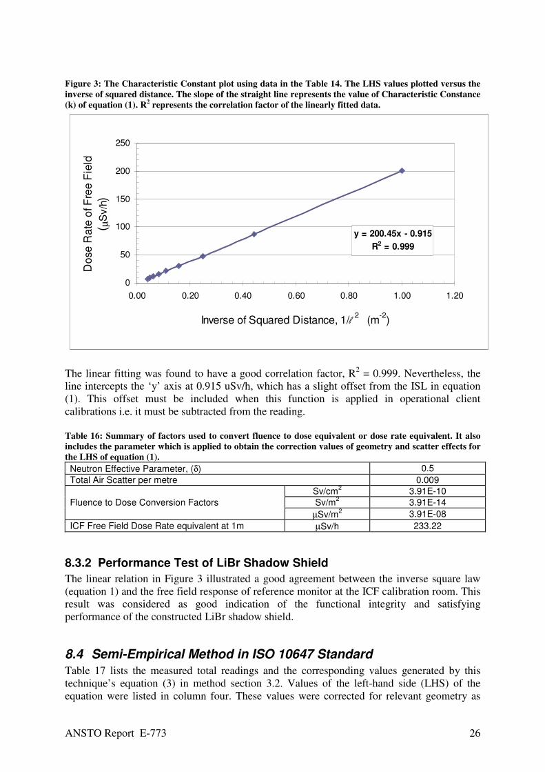
A plot of LHS values of equation (1) versus squared distances is given in Figure 3. The slope
of linearly fitted data was 200.4 µSv/h, which corresponded to the Characteristic Constant (k)
per neutron fluent rate for the ICF. The fitted function is given by:
y = 200.4 x - 0.915
Where:
‘y’ and ‘x’ represent the corrected monitor reading (Mc) and the inverse of the squared
distance (1/l2) respectively.
† Physikalisch-Technische Bundesanstalt, Germany.
‡ National Physical Laboratory, UK.
ANSTO Report E-773 26
Figure 3: The Characteristic Constant plot using data in the Table 14. The LHS values plotted versus the
inverse of squared distance. The slope of the straight line represents the value of Characteristic Constance
(k) of equation (1). R2 represents the correlation factor of the linearly fitted data.
y = 200.45x - 0.915
R2 = 0.999
0
50
100
150
200
250
0.00 0.20 0.40 0.60 0.80 1.00 1.20
Inverse of Squared Distance, 1/l 2 (m
-2)
Do
se
Ra
te o
f F
ree
Fie
ld
( µS
v/h
)
The linear fitting was found to have a good correlation factor, R2 = 0.999. Nevertheless, the
line intercepts the ‘y’ axis at 0.915 uSv/h, which has a slight offset from the ISL in equation
(1). This offset must be included when this function is applied in operational client
calibrations i.e. it must be subtracted from the reading.
Table 16: Summary of factors used to convert fluence to dose equivalent or dose rate equivalent. It also
includes the parameter which is applied to obtain the correction values of geometry and scatter effects for
the LHS of equation (1).
Neutron Effective Parameter, (δ) 0.5
Total Air Scatter per metre 0.009
Sv/cm2 3.91E-10
Sv/m2 3.91E-14 Fluence to Dose Conversion Factors
µSv/m2 3.91E-08
ICF Free Field Dose Rate equivalent at 1m µSv/h 233.22
8.3.2 Performance Test of LiBr Shadow Shield
The linear relation in Figure 3 illustrated a good agreement between the inverse square law
(equation 1) and the free field response of reference monitor at the ICF calibration room. This
result was considered as good indication of the functional integrity and satisfying
performance of the constructed LiBr shadow shield.
8.4 Semi-Empirical Method in ISO 10647 Standard
Table 17 lists the measured total readings and the corresponding values generated by this
technique’s equation (3) in method section 3.2. Values of the left-hand side (LHS) of the
equation were listed in column four. These values were corrected for relevant geometry as

ANSTO Report E-773 27
well as total air scatter effects. The latter factor is equal to the inscatter minus the outscatter
components. These correction factors used in the equation were listed in column six and eight.
Figure 4 shows a plot of the LHS values (measurements) versus squared distance (l 2) as well
as their linearly fitted function. The linear fitting is given in equation (16) with a correlation
factor of R2 = 0.97. The variables ‘y’ and ‘x’ in the equation represent the corrected value of
the total reading of the ICF reference monitor and the squared distance of source to monitor
respectively.
(16) y = 5.879e-6 x + 1.439e-4
The maximum deviation from linearity was within three percent. This deviation shall be
included as an error when equation (16) is utilised in operational calibration of similar
monitors. This equation was rearranged to obtain the fractional room return scatter (S) =
0.041 and the fluence rate response=1.439e-4 (monitor reading per n/m2). The resulted new
format is given in equation 17. This S value agreed with the that obtained by NCRP 112
method with 93.2% (S = 0.044, section 8.6.2).
(17) y = 1.439e-4 (1+ 0.041 x)
Hence, the corresponding monitor reading, induced by the free field of ICF neutron fluence
(i.e. 1.657e6 n/m2) at 1 metre, was calculated as follows.
Monitor Reading =1.439e-4 x 1.657e6 = 238.44 µµµµSv/h
This response of the ICF reference monitor must be traced to an acceptable standard authority
e.g. PTB§, NPL
**…
Table 17: Monitor readings (LHS of equation 3) and the applied correction values of air scatter and
geometry at different distances between the neutron source and monitor.
Distance, llll
(m)
Total Reading
(µµµµSv/5min)
Total Reading,
MT
(µµµµSv/h)
LHS of Eq.3
(µµµµSv/h per n/m
2)
llll 2
(m2)
Air-Inscatter,
(1+A*llll)
Fluence
(n/m2)
Geometry Factor,
F1(llll)
1 19.213 230.554 1.38E-04 1.00 1.009 1.657E+06 1.0014
1.5 9.303 111.631 1.49E-04 2.25 1.0135 7.364E+05 1.0006
2 5.715 68.585 1.63E-04 4.00 1.018 4.142E+05 1.0004
2.5 4.104 49.248 1.82E-04 6.25 1.0225 2.651E+05 1.0002
3 3.169 38.028 2.01E-04 9.00 1.027 1.841E+05 1.0002
3.5 2.560 30.718 2.20E-04 12.25 1.0315 1.353E+05 1.0001
4 2.092 25.109 2.34E-04 16.00 1.036 1.036E+05 1.0001
4.5 1.786 21.432 2.52E-04 20.25 1.0405 8.182E+04 1.0001
5 1.546 18.550 2.68E-04 25.00 1.045 6.627E+04 1.0001
§ Physikalische-Technische Bundesanstalt (PTB) in Germany.
** National Physical Laboratory in UK.

ANSTO Report E-773 28
Figure 4: Plot of the semi empirical method results given in Table 17 (fourth and fifth columns). LHS
values were plotted versus the corresponding squared distance (llll 2). The data were also fitted into a linear
function of correlation factor R2 = 0.97.
y = 5.879E-06x + 1.439e-4
R² = 0.97
0.0E+00
5.0E-05
1.0E-04
1.5E-04
2.0E-04
2.5E-04
3.0E-04
0 5 10 15 20 25 30
Distance Squared, l l l l 2 (m
2)
Flu
en
ce R
ate
Resp
on
se,
LH
S
(µµ µµ
Sv/h
) /
(n/m
2)
ISO 10647 standard3 recommends that the scatter component in a neutron-calibration field
should not exceed 40 percent. Thus, the obtained S value of the ICF calibration room was
translated to a maximum calibration distance (l) = 3.12m. The details of calculations are
provided below:
S x l l l l 2 should be less or equal 40%
0.041 x llll 2 =<40/100
llll = √√√√ (0.4/0.041) = 3.12m
A summary of the obtained values by the semi empirical method of ISO 10647 standard is
shown in Table 18 below.
Table 18: The Fractional Room Return Scatter at the ICF calibration room, obtained by using the ISO
10647 Semi Empirical method. Also listed are the in situ calibration factor (CF), the fluence and dose rate
responses of the ICF reference monitor.
Fluence Response,
Rφφφφ [Measured]
(µµµµSv/h) per( n/m2)
CF
(µµµµSv/h) per
(Nominal
µµµµSv/h)
Response of Dose
Rate Equivalent, RΗΗΗΗ
(Nominal µµµµSv/h)
per (µµµµSv/h)
Fluence Rate
Response, hφφφφ [reference]
(µµµµSv/h/m2)
Fractional Room Return Scatter, S
1.439E-04 0.98 1.02 1.41E-04 0.041

ANSTO Report E-773 29
8.5 Polynomial Fit Method in ISO 10647 Standard
The measurement results by this method are listed in Table 19. The values of left hand side of
equation (4), listed in column six, were obtained by dividing the total reading (MT) over the
product of neutron fluence and geometry factor, F1(l). These values were then fitted into a
second degree polynomial function to determine the function’s coefficient constants.
The RHS values were generated from the characterised polynomial function, which
represented the predicted responses of ICF reference monitor versus distances. Obviously, the
correction for total air scatter effect, i.e. inscatter minus outscatter, was incorporated within
the polynomial coefficients.
The data provided in bold font was used in the polynomial fitting assessment using the Power
Matrix LSM.
Table 19: A list of total readings and the relevant generated values of RHS of equation (4) of the
polynomial technique given in 3.3. The data provided in bold was used in the polynomial fitting
assessment of Power Matrix LSM.
Distance, llll
(m)
llll 2
(m2)
Total Reading,
MT
(µµµµSv/h)
Geometry Factor,
F1(l)
Fluence
(n/m2)
LHS
(µµµµSv/h per n/m
2)
RHS
(Forsythe Analysis)
%∆∆∆∆ of RHS to
LHS
1 1 2.306E+02 1.0014 1.657E+06 1.389E-04 1.360E-04 2.09
1.5 2.25 1.116E+02 1.0006 7.364E+05 1.515E-04 1.526E-04 -0.75
2 4 6.858E+01 1.0004 4.142E+05 1.655E-04 1.697E-04 -2.51
2.5 6.25 4.925E+01 1.0002 2.651E+05 1.857E-04 1.872E-04 -0.77
3 9 3.803E+01 1.0002 1.841E+05 2.065E-04 2.051E-04 0.69
3.5 12.25 3.072E+01 1.0001 1.353E+05 2.271E-04 2.235E-04 1.58
4 16 2.511E+01 1.0001 1.036E+05 2.424E-04 2.424E-04 0.04
4.5 20.25 2.143E+01 1.0001 8.182E+04 2.619E-04 2.617E-04 0.10
5 25 1.855E+01 1.0001 6.627E+04 2.799E-04 2.814E-04 -0.55
8.5.1 Forsythe Orthogonal Fitting
The values of LHS were fitted into a second degree polynomial function versus distance (l) to
determine the function coefficient constants using the Forsythe Orthogonal Method (Figure
5). The resulted polynomial function was rearranged in order to determine the fluence rate
response (hφ), i.e. to match the same format given in equation (5). Both function’s forms are
given below, where ‘x’ represents the distance (l) and ‘y’ represents the RHS value.
y = 1.042e-4 + 3.092e-5 x + 9.038e-7 x2
or
y = 1.042e-4 (1 + 2.966e-1 x + 8.671e-3 x2)
From the above equation, the fluence response (Rφ) for the ICF reference monitor (in situ)
corresponded to 1.042e-4 (monitor reading per n/m2). Furthermore, the corresponding value
of the monitor reading that was induced by the free field of the ICF neutron fluence (i.e.
1.657e6 n/m2) at 1 metre was calculated as follows.
Monitor Reading =1.042e-4 x 1.657e6 = 172.66 µµµµSv/h
ANSTO Report E-773 30
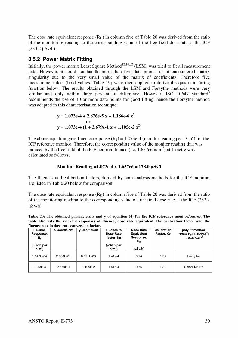
The dose rate equivalent response (RH) in column five of Table 20 was derived from the ratio
of the monitoring reading to the corresponding value of the free field dose rate at the ICF
(233.2 µSv/h).
8.5.2 Power Matrix Fitting
Initially, the power matrix Least Square Method12,14,22
(LSM) was tried to fit all measurement
data. However, it could not handle more than five data points, i.e. it encountered matrix
singularity due to the very small value of the matrix of coefficients. Therefore five
measurement data (bold values, Table 19) were then applied to derive the quadratic fitting
function below. The results obtained through the LSM and Forsythe methods were very
similar and only within three percent of difference. However, ISO 10647 standard3
recommends the use of 10 or more data points for good fitting, hence the Forsythe method
was adapted in this characterisation technique.
y = 1.073e-4 + 2.876e-5 x + 1.186e-6 x2
or
y = 1.073e-4 (1 + 2.679e-1 x + 1.105e-2 x2)
The above equation gave fluence response (Rφ) = 1.073e-4 (monitor reading per n/ m2) for the
ICF reference monitor. Therefore, the corresponding value of the monitor reading that was
induced by the free field of the ICF neutron fluence (i.e. 1.657e6 n/ m2) at 1 metre was
calculated as follows.
Monitor Reading =1.073e-4 x 1.657e6 = 178.0 µµµµSv/h
The fluences and calibration factors, derived by both analysis methods for the ICF monitor,
are listed in Table 20 below for comparison.
The dose rate equivalent response (RH) in column five of Table 20 was derived from the ratio
of the monitoring reading to the corresponding value of free field dose rate at the ICF (233.2
µSv/h).
Table 20: The obtained parameters x and y of equation (4) for the ICF reference monitor/source. The
table also lists the relevant responses of fluence, dose rate equivalent, the calibration factor and the
fluence rate to dose rate conversion factor. Fluence
Response,
Rφφφφ
(µµµµSv/h per n/m
2)
X Coefficient y Coefficient Fluence to Dose Rate
factor, hφφφφ
(µµµµSv/h per n/m
2)
Dose Rate Equivalent Response,
RH
(µµµµSv/h)
Calibration Factor, CF
poly-fit method
RHS= Rφφφφ.(1+x.llll+y.l l l l 2)
= a+b.l l l l +c.llll 2
1.042E-04 2.966E-01 8.671E-03 1.41e-4 0.74 1.35 Forsythe
1.073E-4 2.679E-1 1.105E-2 1.41e-4 0.76 1.31 Power Matrix

ANSTO Report E-773 31
Figure 5: Plots of LHS and RHS values versus distances. R
2 represents the correlation coefficient of fitted
data (RHS values). The equation of monitor response as a function of distance (llll) is also listed.
y = 9.037E-07x2 + 3.091E-05x + 1.042E-04
R2 = 9.977E-01
0.0E+00
5.0E-05
1.0E-04
1.5E-04
2.0E-04
2.5E-04
3.0E-04
0 1 2 3 4 5 6
Distance, llll (m)
Flu
en
ce R
ate
Re
spo
nse
, LH
S
(µµ µµ
Sv
/hr)
/ (
n/m
2)
Response=1.042e-4(1+0.297 l +0.009 l 2)
8.6 Shadow Method in NCRP5,4 112 Report
8.6.1 Fractional Dose Rate of Free Field Neutrons
The component of direct neutron fluence, impinging on the monitor, was deduced by taking
the difference between the Total and Shadowed readings. The fractions of direct dose rates are
the ratio of direct to the total readings as a function of corresponding distances and are listed
in Table 21. The fractional dose rates and their associated combined standard deviations (SD)
were also listed. The error propagation formula15,16,17
was applied to obtain the combined
standard deviation. A plot of these fractions versus distances (l) is illustrated in Figure 6.
The air scatter correction factor was neither applied to the total nor to the ‘direct’ readings
because it would cancel out as a reading ratio.
Table 21: Values of dose rate fractions of free field neutrons (direct) at the ICF calibration room. These
fractions represented the ratio of direct to total doses recorded by the ICF reference monitor at various
distances (llll). The SD represents the combined statistical standard deviation. Distance,
llll
(m)
Total Reading
(µµµµSv/5min)
Shadow Reading
(µµµµSv/5min)
Readings Difference
(µµµµSv/5min)
SD of Difference
(µµµµSv/5min)
Fraction of Direct
Dose Rate
SD of Fraction
%SD of Fraction
1 19.213 2.620 16.593 0.162 0.864 0.011 1.3
1.5 9.303 2.192 7.111 0.136 0.764 0.018 2.4
2 5.715 1.800 3.916 0.055 0.685 0.011 1.6
2.5 4.104 1.581 2.523 0.065 0.615 0.018 2.9
3 3.169 1.422 1.747 0.046 0.551 0.016 3.0
3.5 2.560 1.244 1.316 0.042 0.514 0.017 3.4
4 2.092 1.148 0.945 0.063 0.451 0.032 7.2
4.5 1.786 1.023 0.763 0.050 0.427 0.029 6.9
5 1.546 0.926 0.620 0.040 0.401 0.027 6.6
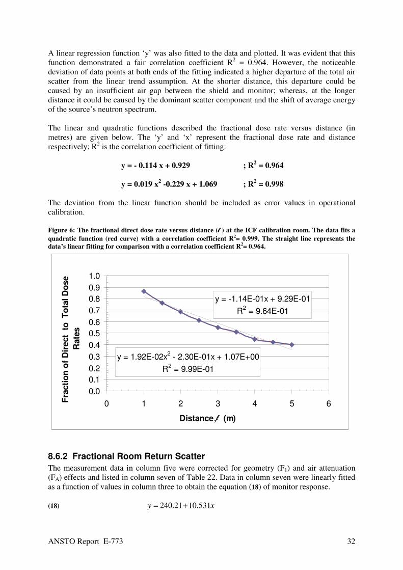
ANSTO Report E-773 32
A linear regression function ‘y’ was also fitted to the data and plotted. It was evident that this
function demonstrated a fair correlation coefficient R2 = 0.964. However, the noticeable
deviation of data points at both ends of the fitting indicated a higher departure of the total air
scatter from the linear trend assumption. At the shorter distance, this departure could be
caused by an insufficient air gap between the shield and monitor; whereas, at the longer
distance it could be caused by the dominant scatter component and the shift of average energy
of the source’s neutron spectrum.
The linear and quadratic functions described the fractional dose rate versus distance (in
metres) are given below. The ‘y’ and ‘x’ represent the fractional dose rate and distance
respectively; R2 is the correlation coefficient of fitting:
y = - 0.114 x + 0.929 ; R2 = 0.964
y = 0.019 x2 -0.229 x + 1.069 ; R
2 = 0.998
The deviation from the linear function should be included as error values in operational
calibration.
Figure 6: The fractional direct dose rate versus distance (llll ) at the ICF calibration room. The data fits a
quadratic function (red curve) with a correlation coefficient R2= 0.999. The straight line represents the
data’s linear fitting for comparison with a correlation coefficient R2= 0.964.
y = -1.14E-01x + 9.29E-01
R2 = 9.64E-01
y = 1.92E-02x2 - 2.30E-01x + 1.07E+00
R2 = 9.99E-01
0.0
0.1
0.2
0.3
0.4
0.5
0.6
0.7
0.8
0.9
1.0
0 1 2 3 4 5 6
Distance,llll (m)
Fra
cti
on
of
Dir
ect
to
T
ota
l D
ose
Rate
s
8.6.2 Fractional Room Return Scatter
The measurement data in column five were corrected for geometry (F1) and air attenuation
(FA) effects and listed in column seven of Table 22. Data in column seven were linearly fitted
as a function of values in column three to obtain the equation (18) of monitor response.
(18) xy 531.1021.240 +=
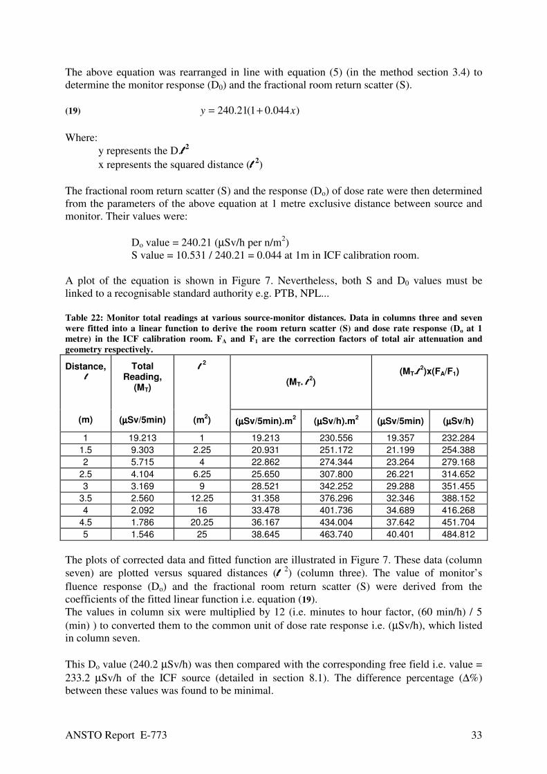
ANSTO Report E-773 33
The above equation was rearranged in line with equation (5) (in the method section 3.4) to
determine the monitor response (D0) and the fractional room return scatter (S).
(19) )044.01(21.240 xy +=
Where:
y represents the D.llll 2
x represents the squared distance (l l l l 2)
The fractional room return scatter (S) and the response (Do) of dose rate were then determined
from the parameters of the above equation at 1 metre exclusive distance between source and
monitor. Their values were:
Do value = 240.21 (µSv/h per n/m2)
S value = 10.531 / 240.21 = 0.044 at 1m in ICF calibration room.
A plot of the equation is shown in Figure 7. Nevertheless, both S and D0 values must be
linked to a recognisable standard authority e.g. PTB, NPL...
Table 22: Monitor total readings at various source-monitor distances. Data in columns three and seven
were fitted into a linear function to derive the room return scatter (S) and dose rate response (Do at 1
metre) in the ICF calibration room. FA and F1 are the correction factors of total air attenuation and
geometry respectively.
(MT. llll 2)
(MT.llll
2)x(FA/F1)
Distance, llll
(m)
Total Reading,
(MT)
(µµµµSv/5min)
llll 2
(m2) ((((µµµµSv/5min).m
2 (µµµµSv/h).m
2 (µµµµSv/5min) (µµµµSv/h)
1 19.213 1 19.213 230.556 19.357 232.284
1.5 9.303 2.25 20.931 251.172 21.199 254.388
2 5.715 4 22.862 274.344 23.264 279.168
2.5 4.104 6.25 25.650 307.800 26.221 314.652
3 3.169 9 28.521 342.252 29.288 351.455
3.5 2.560 12.25 31.358 376.296 32.346 388.152
4 2.092 16 33.478 401.736 34.689 416.268
4.5 1.786 20.25 36.167 434.004 37.642 451.704
5 1.546 25 38.645 463.740 40.401 484.812
The plots of corrected data and fitted function are illustrated in Figure 7. These data (column
seven) are plotted versus squared distances (llll 2) (column three). The value of monitor’s
fluence response (Do) and the fractional room return scatter (S) were derived from the
coefficients of the fitted linear function i.e. equation (19).
The values in column six were multiplied by 12 (i.e. minutes to hour factor, (60 min/h) / 5
(min) ) to converted them to the common unit of dose rate response i.e. (µSv/h), which listed
in column seven.
This Do value (240.2 µSv/h) was then compared with the corresponding free field i.e. value =
233.2 µSv/h of the ICF source (detailed in section 8.1). The difference percentage (∆%)
between these values was found to be minimal.

ANSTO Report E-773 34
∆∆∆∆% = [(233.2 – 240.2)/233.2]x100 = -3%
A summary of the S and D0 values, obtained by the NCRP 112 method is given in Table 23.
Table 23: Values of S and (D0 = Rφ), obtained by the NCRP 112 method. ‘∆%’ represents the percentage
difference between the monitor response and the free field fluence rate of the ICF neutron source. The
measured response represents the value that was obtained from the fitted linear function. Room Scatter
Factor, S Measured Rφφφφ
(µµµµSv/5min)
Measured Rφφφφ
(µµµµSv/h)
Calculated Rφφφφ
(µµµµSv/h) ∆∆∆∆%Source to
Direct Dose Rates
0.044 20.018 240.216 233.2 -3
Figure 7: Plot of room return scatter: the product of the total reading by squared distance (D.l l l l 2
= MT.l l l l 2)
versus the squared distance (llll 2). The linear fitting has a correlation coefficient R2 = 0.976.
y = 10.531x + 240.21
R2 = 0.9755
0
100
200
300
400
500
600
0 5 10 15 20 25 30
Squared Distance, l l l l 2 (m)
D .
l l l l
2 ,
(µµ µµ
Sv
/h)
.( m
2 )
The ISO 10647 standard3 recommends that the scatter component in a neutron-calibration
field should not exceed 40 percent. This scatter, as a function of distance, is given by the
following equation:
S x llll 2 =< 40%
Thus, the maximum distance (l ) at the ICF rig calibration room that would fulfil this
requirement was calculated as follows.
0.044 x llll 2 =<40/100
Hence,
llll = √√√√ (0.4/0.044) = 3.02m

ANSTO Report E-773 35
8.7 Summary of Fractional Room Return Scatter and Monitor Response
The measured fractional room return scatter S that characterised the ICF calibration room,
using the ICF reference monitor and neuron source of serial number 4232 NE, is listed in
column three of Table 24. The standards and methods which were applied to determine the S
value are listed in columns one and two.
Table 24: Measured values of the fractional room return scatter (S) at the ICF calibration room. The
applied standards and methods are also listed.
Standard Method Fractional Room Return
Scatter, S
NCRP 112 D.l 2 = Do.(1 + S.l 2) 0.044
ISO 10647 Semi-Empirical 0.041
ISO 10647 Shadow Shield
n/a
(incorporated within the
Characteristic Constant k)
ISO 10647 Polynomial n/a
Table 25 lists a summary of the measured responses at 1 metre by the ICF reference monitor
and the applied standards and methods of measurements and analysis.
The values of fluence response in column six were obtained by dividing the monitor reading
(column four) by the neutron fluence (1.657e6 n/m2) of free field at 1 metre in the ICF
calibration room (section 8.1). The values of monitor ‘reading’ in column four were obtained
from the fitted equation of the corresponding method. They included the corrections of air
attenuation and geometry effect when appropriate; the fluence response was multiplied by the
ICF neutron fluence to obtain the monitor reading in column four.
The bolded values in column four were adopted and will be applied in the operational
calibration procedures.
The calibration factors (CF), shown in column six, were obtained by dividing the ICF free
field dose rate at 1metre (i.e. 233.2 µSv/h) by the corresponding values of monitor reading
given in column four. These factors represented the in situ values and must be linked to a
recognisable standard authority for traceability e.g. PTB, NPL...
Table 25: Summary of measured monitor responses at 1 metre by the ICF reference monitor. Also listed
are the applied standards, methods and fitting analysis. The in situ calibration factors (CF) of the ICF
reference monitor are shown in the last column.
Methods
Standard
Measurement Analysis
Monitor Reading
@1m
((((µµµµSv/h)
Fluence Response
(nominal
µµµµSv/h) per (n/m
2)
Calibration Factor, CF
(µSv per
nominal µSv)
NCRP 112 D.llll 2 = Do.(1 + S.llll 2) Forsythe 240.12 1.449E-04 0.97
ISO 10647 shadow Forsythe 200.40 1.210E-04 1.16
ISO 10647 semi-empirical Forsythe 245.24 1.480E-04 0.95

ANSTO Report E-773 36
ISO 10647 semi-empirical Excel 97 238.44 1.439E-04 0.98
ISO 10647 polynomial 10 points Forsythe
172.66 1.042E-04 1.35
ISO 10647 polynomial 5 points Power Matrix
178.0 1.073E-04 1.31
Reference Values:
fluence to dose conversion factor at ICF, [µµµµSv/h per n/m
2]
Section 8.1 1.407e-4
fluence to dose conversion factor at ICF, [n/m2
per µµµµSv/h] 1/1.407e-4 7.104e+3
ICF free field fluence at 1m, [n/m2] Section 8.1 1.657e+6
ICF free field dose rate at 1m [µµµµSv/h] Section 8.1 233.2
9 Discussion An aqueous LiBr shadow shield (cone) was designed and constructed. The properties of
involved materials were evaluated e.g. neutron absorption and scattering. The geometry,
described in the NCRP 112 Report, was adopted in this design. Also, the evaluation included
the comparison of neutron diffusion length between LiBr and Li2CO3 compounds.
The deviation from the construction and utilisation of the Li2CO3 wax cone, as described in
the report, was prompted by the technical difficulties and poor quality of the initial
manufactured cone (e.g. non uniformity of neutron absorber particulates, air voids, time
constrain and manufacturing delay…).
The evaluation (detailed in section 5.2) showed that the cone with the LiBr compound
possessed seven percent higher absorption and 31 percent less scatter cross sections to
neutrons, compared with the Li2CO3 cone. Consequently, the LiBr cone should cause less
scattering and more absorption to the direct impinging neutrons than the Li2CO3 cone
(advantage). Furthermore, the higher absorption feature reduces the available direct neutrons
for scattering.
In addition water (as solvent) possesses a short Diffusion Length23
(L = a few centimetres)
and therefore the majority of the scattered neutrons would take place within the solution and
eventually be absorbed with minimal additional scatter outside the cone. The presence of C
and O atoms in the moderating materials (water or wax) of both cone types should have
insignificant effects due to their very large L values.
It was found that the alternative shadow shield with the LiBr solution had several advantages
such as ready availability, the low cost of construction materials and the simple and
straightforward steps of solution reparation and cone-shell fabrication.
Performance tests carried out on the LiB aqueous shield (cone) illustrated that the direct
neutron fluence (difference between total and scattered neutrons) followed the ‘inverse square
law’ quite well, with a correlation factor =0.999 (see Figure 3 ).

ANSTO Report E-773 37
The values of the fractional room return scatter (S), determined by the semi-empirical of
ISO10647 and shadow shield of NRCP112, were in reasonable agreement within seven
percent (see Table 24).
The size of the ICF calibration room fulfils the requirement by the shadow shield method i.e.
a medium to a large size room (see appendices). Also, the fluence responses were relatively in
good agreement with the calculated value from the source certificate; the resulted values of
Characteristic Constant k and S, had good fitting’s correlation coefficient. Therefore, these
values were adopted for operational calibration services.
The S value at the ICF calibration room changes as a function of the second degree
polynomial of distance. So beyond about three metres in distance the corresponding S value
exceeds 40 percent of the recommended scatter limit by ISO 10647 (to avoid significant
change to the neutron energy spectrum of the 241
Am/Be source). Notably, this distance is 90
percent of the radius between the source-guide tube and room walls (see Figure 2). This
suggests that the room floor contributes more scatter than the walls. Thus a further increase in
source height would reduce the floor scatter and ultimately the overall scatter (e.g. floor and
walls). However, other competing factors should be carefully considered in such a decision,
like the convenience of the instrument’s set up, the frequency / demand for such a distance
(e.g. low dose/rate), the cost to build an off ground calibration platform etc…
All parameters obtained in the ICF characterisation should be linked to a recognisable
standard authority e.g. PTB, NPL…
The ICF reference monitor showed variations in the values of responses and calibration
factors which were clearly dependent on the applied method. A summary of these values is
provided in Table 25.
A comparison between the calibration factor (in situ, obtained in this work) of the ICF
reference monitor with a traceable calibration by a recognisable standard authority (e.g. PTB,
NPL…) of the same monitor should give an insight into the integrity of the current neutron
source in the ICF rig. It also provides a practical way to validate its emission versus
calibration certificate.
The values of a free field dose rate of 16.2mSv/h, 3.7mSv/h and 0.933 mSv/h, corresponding
to the distances of 0.12m, 0.25m and 0.5m respectively (in Table 11), were obtained by
extrapolation calculations. They will provide extra calibration capability at the ICF rig
calibration room which is required by some clients. However, it should be noted that these
dose rates are still well below the upper-end of the recommended3 dose rate by the ISO 10647
standard (i.e. 40mSv/h for neutron calibration facility, radiological applications).
The standard also recommends 10µSv/h at the lower-end of dose rate range. Such a dose rate
would be achieved at distance of about 5 metres in the ICF rig calibration room. However,
this distance is beyond the maximum distance limit for 40 percent of scattered neutrons and
should be avoided.
In order to comply with the standard an alternative solution would be the installation of two
neutron sources in the ICF rig. Their activities shall be carefully chosen to provide the
recommended dose rates within the recommend distance range3 i.e.=<40% scattered neutrons.

ANSTO Report E-773 38
Different fitting methods illustrated a slight effect on the coefficients of fitted quadratic
equations, which mainly affects the monitor response value (see Table 25). Overall, all fitting
methods give comparable linear results (about four percent).
Equations linearly fitted by Forsythe or Excel data analysis technique gave comparable
results.
The calibration stand, attached to the moving rail, was wobbly and shall be rectified; the
vertical deviation must not exceed 2mm.
The arithmetical mean and sample standard deviation (SD) of five repeated measurements
were used to represent the average reading and its associated statistical dispersion. The
uncertainty propagation technique was applied to obtain the combined uncertainty (A type) of
a given measurement technique’s function.
The agreement of fitted functions with the hypothesis of the measurement analysis was
considered as an illustration of good accuracy with measurement16
. Furthermore the accuracy
of linear slope, used to obtain the monitor response, should be verified with the corresponding
traceable value of monitor response (when available).
A Maximum Likelihood Test16
(χ2 Parameter) would provide an index of accuracy between
the hypothesis and measurement but would require a large set of data and counts which was
not possible to apply to this work due to time constraints. The uncertainty scope given in ISO
10647 is still applicable to this work and should be considered as Type B15,17
.
Recording devices for temperature, pressure and humidity should be installed in the ICF
calibration room. Additional shadow shields of smaller sizes are required to characterise
different geometries.
It is recommended to explore an appropriate mechanism / adaptor fitting at the top of the
source-tube, so the anisotropy check of the source can be carried out easily and regularly for
QA fulfilment.
It is worth noticing that at the completion of this characterisation and report, the calibration
results with the Physikalische-Technische Bundesanstalt (PTB) in Germany became available.
As a result, the neutron characterisation at ICF calibration room did agree with the BTP
calibration within five percent. Consequently, the neutron field in ICF rig calibration room is
now traceable to BTP standard laboratory in Germany. Also, this agreement confirms the
integrity of the current neutron source e.g. anisotropy stability, which should save substantial
cost and efforts in replacing the source or sending it overseas for re-certification.
The details of the results comparison as well as copy of the PTB calibration report are given
in appendices 11.3 and 11.4.

ANSTO Report E-773 39
10 Conclusions
• The Fractional Room Return Scatter (S) at the ICF calibration room was determined.
The small S value illustrated a good quality feature of the room.
• The measured S Values by NCRP112 or ISO10647 methods were in good agreement
(93 percent).
• Operational calibrations should be carried out within three metres distance from the
neutron source in order to comply with 40 percent of the room scatter limit;
recommended by the ISO 10647 standard3.
• The new type of aqueous LiBr truncated cone was successfully implemented in
measurements by the shadow shield technique.
• The fluence and dose rate equivalent responses (in situ) were determined for the ICF
reference monitor. The reference neutron fluence was taken from the source
certificate. Hence, the responses must be linked to a recognisable standard authority
e.g. PTB, NPL… for legal traceability requirements.
• Three extra positions of relatively high dose rates were determined. They will expand
the capability of dose rate range at the ICF calibration service that are desired by some
clients.
• The reference neutron fluence given in the source’s certificate should be compared
with the corresponding value provided by the standard authority as a measure of the
source’s integrity at the rig calibration room.
• The characteristic parameters measured by the different techniques were evaluated and
the appropriate ones identified for implementation at the ICF calibration room.
Furthermore the relevant operational instructions should be developed for future
routine calibrations.
• The facility currently lacks a high dose rate range (recommended3 by the ISO 10647
Standard) that is usually available at similar facilities.
• The ICF should have two neutron sources of appropriate activities to achieve the
recommended3 dose rate range.
• Additional shadow shields are required for other characterisation geometries in future.
• The neutron field at ICF rig room becomes now traceable to the Physikalische-
Technische Bundesanstalt (PTB) in Germany. The calibration result by this standard
authority became available after the completion of this characterisation and report.
ICF results did agree with PTB calibration within five percent.
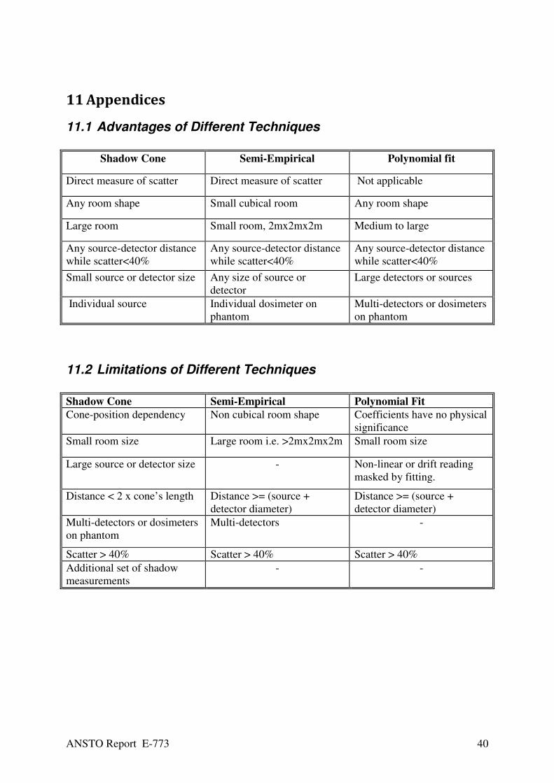
ANSTO Report E-773 40
11 Appendices
11.1 Advantages of Different Techniques
Shadow Cone Semi-Empirical Polynomial fit
Direct measure of scatter Direct measure of scatter Not applicable
Any room shape Small cubical room Any room shape
Large room Small room, 2mx2mx2m Medium to large
Any source-detector distance
while scatter<40%
Any source-detector distance
while scatter<40%
Any source-detector distance
while scatter<40%
Small source or detector size Any size of source or
detector
Large detectors or sources
Individual source Individual dosimeter on
phantom
Multi-detectors or dosimeters
on phantom
11.2 Limitations of Different Techniques
Shadow Cone Semi-Empirical Polynomial Fit
Cone-position dependency Non cubical room shape Coefficients have no physical
significance
Small room size Large room i.e. >2mx2mx2m Small room size
Large source or detector size - Non-linear or drift reading
masked by fitting.
Distance < 2 x cone’s length Distance >= (source +
detector diameter)
Distance >= (source +
detector diameter)
Multi-detectors or dosimeters
on phantom
Multi-detectors -
Scatter > 40% Scatter > 40% Scatter > 40%
Additional set of shadow
measurements
- -
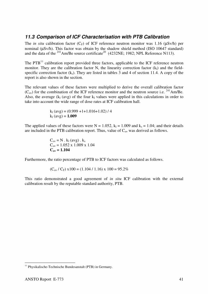
ANSTO Report E-773 41
11.3 Comparison of ICF Characterisation with PTB Calibration
The in situ calibration factor (CF) of ICF reference neutron monitor was 1.16 (µSv/h) per
nominal (µSv/h). This factor was obtain by the shadow shield method (ISO 10647 standard)
and the data of the 241
Am/Be source certificate20
(4232NE; 1982; NPL Reference N113).
The PTB††
calibration report provided three factors, applicable to the ICF reference neutron
monitor. They are the calibration factor N, the linearity correction factor (kl) and the field-
specific correction factor (ks). They are listed in tables 3 and 4 of section 11.4. A copy of the
report is also shown in the section.
The relevant values of these factors were multiplied to derive the overall calibration factor
(Cov) for the combination of the ICF reference monitor and the neutron source i.e. 241
Am/Be.
Also, the average (kl (avg) of the four kl values were applied in this calculations in order to
take into account the wide range of dose rates at ICF calibration hall.
kl (avg) = (0.999 +1+1.016+1.02) / 4
kl (avg) = 1.009
The applied values of these factors were N = 1.052, kl = 1.009 and ks = 1.04; and their details
are included in the PTB calibration report. Thus, value of Cov was derived as follows.
Cov = N . kl (avg) . ks
Cov = 1.052 x 1.009 x 1.04
Cov = 1.104
Furthermore, the ratio percentage of PTB to ICF factors was calculated as follows.
(Cov / CF) x100 = (1.104 / 1.16) x 100 = 95.2%
This ratio demonstrated a good agreement of in situ ICF calibration with the external
calibration result by the reputable standard authority, PTB.
††
Physikalische-Technische Bundesanstalt (PTB) in Germany.

ANSTO Report E-773 42
11.4 PTB Calibration Certificate of ICF Reference Monitor

ANSTO Report E-773 43

ANSTO Report E-773 44

ANSTO Report E-773 45
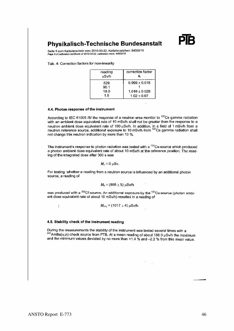
ANSTO Report E-773 46

ANSTO Report E-773 47
ANSTO Report E-773 48

ANSTO Report E-773 49
List of Tables
TABLE 1: SPECIFICATIONS SUMMARY OF THE LIBR COMPOUND USED IN THE SOLUTION
PREPARATION OF A THERMAL NEUTRON ABSORBER............................................................. 9
TABLE 2: W/W% OF IMPURITIES IN ALUMINIUM SHEETS USED IN THE FABRICATION OF THE CONE
SHELL AND TRAYS. THE MACROSCOPIC CROSS SECTIONS OF THESE IMPURITIES ARE MUCH
LESS THAN THE ALUMINIUM. ............................................................................................. 10
TABLE 3: W/W% OF IMPURITIES IN ALUMINIUM RODS TYPE WHICH ARE USED IN FABRICATION OF
THE SUPPORT STAND. THE MACROSCOPIC CROSS SECTIONS OF THESE IMPURITIES ARE MUCH
LESS THAN THE ALUMINIUM. ............................................................................................. 11
TABLE 4: W/W% OF IMPURITIES IN IRON INGOT TYPE WHICH WERE USED IN THE SOLID SECTION
FABRICATION OF THE SHADOW CONE. THE MACROSCOPIC CROSS SECTIONS OF THESE
IMPURITIES WERE MUCH LESS THAN THE IRON (FE). .......................................................... 12
TABLE 5: SPECIFICATIONS OF THE NEUTRON SOURCE IN THE ICF RIG CALIBRATION ROOM. .
MEASUREMENT DATES WERE 4, 8 AND 9 DECEMBER 2009. THE DECAY FACTOR WAS
REFERENCED ON THE MEASUREMENT DATE 8 DECEMBER 2009......................................... 12
TABLE 6: FEATURES OF SHADOW CONE ASSEMBLY. THE ASSEMBLY CONSISTED OF TWO CONICAL
SECTIONS AND A SUPPORTING CRADLE. D1 AND D2 ARE THE DIAMETERS OF THE
TRUNCATED CONES............................................................................................................ 14
TABLE 7: COMPARISON RESULTS OF THE NEUTRON CROSS SECTIONS OF TWO COMPOUNDS USED
AS ABSORBERS OF THERMAL NEUTRON FOR SHADOW CONE. THE LIBR COMPOUND HAS AN
ADVANTAGE OVER LI2CO3 IN TERMS OF LESS SCATTER AND MORE ABSORPTION OF
NEUTRONS. ........................................................................................................................ 15
TABLE 8: COMPARISON RESULTS OF THERMALISED NEUTRON PROPERTIES OF TWO COMPOUNDS
THAT WERE CONSIDERED IN SHADOW SHIELD CONSTRUCTION........................................... 15
TABLE 9: A SUMMARY OF FEATURES AND SPECIFICATIONS OF THE REFERENCE NEUTRON
MONITOR USED AT ICF. ..................................................................................................... 17
TABLE 10: A LIST OF AIR ATTENUATION (FA), GEOMETRY (F1) AND CORRECTION FACTORS AS A
FUNCTION OF THE EFFECTIVE DISTANCE (L) BETWEEN NEUTRON SOURCES AND THE
MONITOR. ALSO, PARAMETERS USED IN THE CALCULATIONS ARE ALSO LISTED: ............... 18
TABLE 11: LIST OF THE FLUENCES AND DOSE RATES OF THE NEUTRON SOURCE (4232 NE) AT
THE ICF RIG CALIBRATION ROOM. THE FREE FIELD VALUES OF NEUTRON FLUENCES IN
COLUMN TWO WERE MULTIPLIED BY *H(10) TO CONVERT THEM TO THE CORRESPONDING
DOSE RATES AND GIVEN IN COLUMN SIX. THE VALUES IN COLUMN FOUR REPRESENT THE
ATTENUATED DOSE RATES (COLUMN THREE VALUES DIVIDED THE CORRESPONDENCE
VALUES OF THE AIR ATTENUATION CORRECTION FACTOR FA(L ) GIVEN IN COLUMN FIVE). . 21
TABLE 12: LIST OF THE INITIAL READING VALUES BY THE ICF MONITOR WITH AND WITHOUT THE
SHADOW SHIELD. THE TOTAL DOSE RATE CORRESPONDED TO THE DIRECT AND SCATTERED
NEUTRONS DETECTED BY THE MONITOR. THE SHADOW DOSE RATE CORRESPONDS TO THE
SCATTERED NEUTRONS ONLY. ........................................................................................... 22
TABLE 13: LIST OF THE AVERAGE DOSE RATE READINGS OF TOTAL AND SHADOW
CONFIGURATIONS OBTAINED BY THE ICF NEUTRON MONITOR. THEIR ASSOCIATED SAMPLE
STANDARD DEVIATIONS (SD) WERE ALSO LISTED.............................................................. 23
TABLE 14: TOTAL AND NET READINGS (TOTAL AND SHADOW) OF THE MONITOR AT DIFFERENT
DISTANCES TO THE NEUTRON SOURCE. THE LAST COLUMN LISTS THE CORRESPONDING
VALUES OF THE LEFT-HAND SIDE (LHS) OF EQUATION (1). ............................................... 24

ANSTO Report E-773 50
TABLE 15: THE VALUES OF MEASURED K AND THE CERTIFICATE’S FREE FIELD FOR THE ICF
REFERENCE MONITOR AT 1 METRE. THIS K CONSTANT CHARACTERISED THE MONITOR, THE
NEUTRON SOURCE AND THE CALIBRATION ROOM AS ONE SYSTEM. Rφ IS THE FREE FIELD
FLUENCE RESPONSE. .......................................................................................................... 25
TABLE 16: SUMMARY OF FACTORS USED TO CONVERT FLUENCE TO DOSE EQUIVALENT OR DOSE
RATE EQUIVALENT. IT ALSO INCLUDES THE PARAMETER WHICH IS APPLIED TO OBTAIN THE
CORRECTION VALUES OF GEOMETRY AND SCATTER EFFECTS FOR THE LHS OF EQUATION
(1). .................................................................................................................................... 26
TABLE 17: MONITOR READINGS (LHS OF EQUATION 3) AND THE APPLIED CORRECTION VALUES
OF AIR SCATTER AND GEOMETRY AT DIFFERENT DISTANCES BETWEEN THE NEUTRON
SOURCE AND MONITOR. ..................................................................................................... 27
TABLE 18: THE FRACTIONAL ROOM RETURN SCATTER AT THE ICF CALIBRATION ROOM,
OBTAINED BY USING THE ISO 10647 SEMI EMPIRICAL METHOD. ALSO LISTED ARE THE IN
SITU CALIBRATION FACTOR (CF), THE FLUENCE AND DOSE RATE RESPONSES OF THE ICF
REFERENCE MONITOR. ....................................................................................................... 28
TABLE 19: A LIST OF TOTAL READINGS AND THE RELEVANT GENERATED VALUES OF RHS OF
EQUATION (4) OF THE POLYNOMIAL TECHNIQUE GIVEN IN 3.3. THE DATA PROVIDED IN
BOLD WAS USED IN THE POLYNOMIAL FITTING ASSESSMENT OF POWER MATRIX LSM. .... 29
TABLE 20: THE OBTAINED PARAMETERS X AND Y OF EQUATION (4) FOR THE ICF REFERENCE
MONITOR/SOURCE. THE TABLE ALSO LISTS THE RELEVANT RESPONSES OF FLUENCE, DOSE
RATE EQUIVALENT, THE CALIBRATION FACTOR AND THE FLUENCE RATE TO DOSE RATE
CONVERSION FACTOR. ....................................................................................................... 30
TABLE 21: VALUES OF DOSE RATE FRACTIONS OF FREE FIELD NEUTRONS (DIRECT) AT THE ICF
CALIBRATION ROOM. THESE FRACTIONS REPRESENTED THE RATIO OF DIRECT TO TOTAL
DOSES RECORDED BY THE ICF REFERENCE MONITOR AT VARIOUS DISTANCES (L). THE SD
REPRESENTS THE COMBINED STATISTICAL STANDARD DEVIATION..................................... 31
TABLE 22: MONITOR TOTAL READINGS AT VARIOUS SOURCE-MONITOR DISTANCES. DATA IN
COLUMNS THREE AND SEVEN WERE FITTED INTO A LINEAR FUNCTION TO DERIVE THE ROOM
RETURN SCATTER (S) AND DOSE RATE RESPONSE (DO AT 1 METRE) IN THE ICF
CALIBRATION ROOM. FA AND F1 ARE THE CORRECTION FACTORS OF TOTAL AIR
ATTENUATION AND GEOMETRY RESPECTIVELY. ................................................................ 33
TABLE 23: VALUES OF S AND (D0 = Rφ), OBTAINED BY THE NCRP 112 METHOD. ‘∆%’
REPRESENTS THE PERCENTAGE DIFFERENCE BETWEEN THE MONITOR RESPONSE AND THE
FREE FIELD FLUENCE RATE OF THE ICF NEUTRON SOURCE. THE MEASURED RESPONSE
REPRESENTS THE VALUE THAT WAS OBTAINED FROM THE FITTED LINEAR FUNCTION. ....... 34
TABLE 24: MEASURED VALUES OF THE FRACTIONAL ROOM RETURN SCATTER (S) AT THE ICF
CALIBRATION ROOM. THE APPLIED STANDARDS AND METHODS ARE ALSO LISTED. ........... 35
TABLE 25: SUMMARY OF MEASURED MONITOR RESPONSES AT 1 METRE BY THE ICF REFERENCE
MONITOR. ALSO LISTED ARE THE APPLIED STANDARDS, METHODS AND FITTING ANALYSIS.
THE IN SITU CALIBRATION FACTORS (CF) OF THE ICF REFERENCE MONITOR ARE SHOWN IN
THE LAST COLUMN. ........................................................................................................... 35

ANSTO Report E-773 51
List of Equations
(1) ∆M . FA(L) = K / L 2
............................................................................................................. 5
(2) K = Rφ . BΩ ........................................................................................................................ 5
(3) MT / [φ . FL(L) . (1 + A . L )] = RΦ (1 + S . L 2) ....................................................................... 5
(4) MT / [φ . FL(L)] = RΦ (1 + X . L + Y . L 2)................................................................................ 6
(5) D. L 2 = DO (1 + S. L
2) ......................................................................................................... 6
(6) PJ+1(X) = (X – αJ+1) PJ(X) –βJ PJ-1(X) .................................................................................. 7
(7)
∑
∑
=
=+
=N
k
N
kk
j
xP
xPxa
kj
kj
1
2
1
2
1
)]([
)]([. ......................................................................................... 7
(8)
∑
∑
=
=
−
−=
N
k
N
kk
j
xP
xPxPx
kj
kjkj
1
2
1
)]([
)().(
1
1.
β............................................................................... 7
(9) Y = B0 . P0(X) + B1 . P1(X) + B2 . P2(X) ................................................................................ 8
(10)
∑
∑
=
==N
k
N
kk
i
xP
xPyb
ki
ki
1
2
1
)]([
)(. ...................................................................................... 8
(11) Y = 0.1818 X + 1 ............................................................................................................. 13
(12) V = π ∫ (0.1818 X + 1) . DX............................................................................................... 13
(13) FA (L,E) = EXP(L..Σ(E))..................................................................................................... 17
(14) F1(L) = 1 + ∆ . (R/2 . L)2
..................................................................................................... 18
(15) K = MC . L 2....................................................................................................................... 25
(16) Y = 5.879E-6 X + 1.439E-4 .............................................................................................. 27
(17) Y = 1.439E-4 (1+ 0.041 X)............................................................................................... 27
(18) xy 531.1021.240 += ..................................................................................................... 32
(19) )044.01(21.240 xy += .................................................................................................. 33
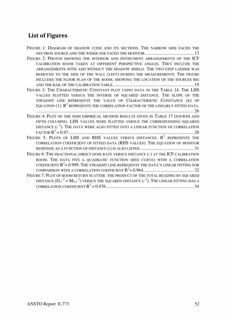
ANSTO Report E-773 52
List of Figures
FIGURE 1: DIAGRAM OF SHADOW CONE AND ITS SECTIONS. THE NARROW SIDE FACED THE
NEUTRON SOURCE AND THE WIDER ONE FACED THE MONITOR........................................... 13
FIGURE 2: PHOTOS SHOWING THE INTERIOR AND INSTRUMENT ARRANGEMENTS OF THE ICF
CALIBRATION ROOM TAKEN AT DIFFERENT PERSPECTIVE ANGLES. THEY INCLUDE THE
ARRANGEMENTS WITH AND WITHOUT THE SHADOW SHIELD. THE TWO-STEP LADDER WAS
REMOVED TO THE SIDE OF THE WALL (LEFT) DURING THE MEASUREMENTS. THE FIGURE
INCLUDES THE FLOOR PLAN OF THE ROOM, SHOWING THE LOCATION OF THE SOURCES RIG
AND THE RAIL OF THE CALIBRATION TABLE. ...................................................................... 19
FIGURE 3: THE CHARACTERISTIC CONSTANT PLOT USING DATA IN THE TABLE 14. THE LHS
VALUES PLOTTED VERSUS THE INVERSE OF SQUARED DISTANCE. THE SLOPE OF THE
STRAIGHT LINE REPRESENTS THE VALUE OF CHARACTERISTIC CONSTANCE (K) OF
EQUATION (1). R2 REPRESENTS THE CORRELATION FACTOR OF THE LINEARLY FITTED DATA.
.......................................................................................................................................... 26
FIGURE 4: PLOT OF THE SEMI EMPIRICAL METHOD RESULTS GIVEN IN TABLE 17 (FOURTH AND
FIFTH COLUMNS). LHS VALUES WERE PLOTTED VERSUS THE CORRESPONDING SQUARED
DISTANCE (L 2). THE DATA WERE ALSO FITTED INTO A LINEAR FUNCTION OF CORRELATION
FACTOR R2 = 0.97.............................................................................................................. 28
FIGURE 5: PLOTS OF LHS AND RHS VALUES VERSUS DISTANCES. R2 REPRESENTS THE
CORRELATION COEFFICIENT OF FITTED DATA (RHS VALUES). THE EQUATION OF MONITOR
RESPONSE AS A FUNCTION OF DISTANCE (L) IS ALSO LISTED. .............................................. 31
FIGURE 6: THE FRACTIONAL DIRECT DOSE RATE VERSUS DISTANCE (L ) AT THE ICF CALIBRATION
ROOM. THE DATA FITS A QUADRATIC FUNCTION (RED CURVE) WITH A CORRELATION
COEFFICIENT R2= 0.999. THE STRAIGHT LINE REPRESENTS THE DATA’S LINEAR FITTING FOR
COMPARISON WITH A CORRELATION COEFFICIENT R2= 0.964. ........................................... 32
FIGURE 7: PLOT OF ROOM RETURN SCATTER: THE PRODUCT OF THE TOTAL READING BY SQUARED
DISTANCE (D.L 2 = MT.L
2) VERSUS THE SQUARED DISTANCE (L
2). THE LINEAR FITTING HAS A
CORRELATION COEFFICIENT R2 = 0.976............................................................................. 34

ANSTO Report E-773 53
References 1 International Standard ISO 8529, Neutron Reference Radiation for Calibrating Neutron-
Measuring Devices used for Radiation Protection Responses and for Determining their
Response as a Function of Neutron Energy; ISO 8529:1989 (E).
2 International Standard ISO 8529-3, Reference Neutron Radiations – Part 3: Calibration of
Area and Personal Dosimeters and Determination of their Response as a Function of Neutron
Energy and Angle of Incidence; ISO 8529-3:1998 (E).
3 International Standard ISO 10647, Procedure for Calibrating and Determining the Response
of Neutron-Measuring Devices used for Radiation Protection Purposes; ISO 10647:1996 (E).
4 Burger, G., Schwartz, R. B., 1988. Guidelines on Calibration of Neutron Measuring
Devices, IAEA Technical Report Series No. 285. International Atomic Energy Agency,
Vienna.
5 Chabot, G. E., et al., 1991. Calibration of Survey Instruments Used in Radiation Protection
for the Assessment of Ionizing Radiation Fields and Radioactive Surface Contamination;
NCRP Report No. 112, National Council on Radiation Protection and Measurements, USA.
6 Hunt, J. B., 1984. The Calibration of Neutron Sensitive Spherical Devices, Radiation
Protection Dosimetry 8(4), 239-251.
7 Eisenhauer, C., M., et al., 1982. Measurement of Neutrons Reflected from the Surfaces of a
Calibration Room, Health Physics 42(4), 489-495.
8 Eisenhauer, C., M., 1989. Review of Scattering Corrections for Calibration of Neutron
Instruments; Radiation Protection Dosimetry 28(4), 253-262.
9 Eisenhauer, C., M., 1985. Calibration Techniques for Neutron Personal Dosimetry,
Radiation Protection Dosimetry 10(1-4), 43-57.
10
Cruz, M. T., Fratin, L., 1992. Establishment of a Procedure for Calibrating Neutron
Monitors at the Physics Institute of the University of Sao Paulo, Brazil, Radiation Protection
Dosimetry 44(1-4), 143-146.
11
Hunt, J. B., 1976. The Calibration and Use of Long Counters for the Accurate Measurement
of Neutron Flux Density; NPL Report RS(EXT)5, ISSN 0143-7135.
12
Pipes, L. A., Harvill, L. R., 1971. Applied Mathematics for Engineering and Physicists, 3rd
Ed., McGraw-Hill International Book Company, 8th
printing 1982.
13
Stroud, K. A., 1982. Engineering Mathematics, Programs & Problems; 2nd
Ed., MacMillan
Press LTD.
14
Southworth, R. W., Deleeuw S. L., 1965. Digital Computation and Numerical Methods.
McGraw-Hill Book Company.

ANSTO Report E-773 54
15
Guide to The Expression of Uncertainty in Measurements (GUM). 1993, 1st Ed., BIPM,
IEC, IFCC, ISO, IUPAC, IUPAP and OIML, ISBN 92-67-10188-9.
16
Caria, M., 2000. Measurement Analysis ‘An Introduction to the Statistical Analysis of
Laboratory Data in Physics, Chemistry and the Life Sciences’. Imperial College Press.
17
Lira, I., 2002. Evaluating the Measurement Uncertainty ‘Fundamental and Practical
Guidance’, Series in Measurement Science and Technology, Institute of Physics Publishing,
Bristol & Philadelphia.
18
Periodical Table, Sergent-Welch Scientific Company, Illinois, USA.
19
Neutron Scattering Length and Cross Section, NIST Center for Neutron Research, USA,
Online: http://www.ncnr.nist.gov/resources/n-lengths/list.html, accessed in June 2009.
20
Certificate of Measurement of 241
Am/Be neutron source, serial No. 4232NE, 1982. NPL
Reference N113.
21
Drawing Reference AOE 116313, ANSTO Engineering, 2006.
22
Wolfram, S., 2003. Mathematical Computing System package, Version 5.
23
Curtiss, L. F., 1959. Introduction to Neutron Physics, D. Van Nostrand Company Inc.
24
Wikipedia online: http://en.wikipedia.org/wiki/paraffin_wax, accessed in June 2009.
25
Neutron Monitor Model 2222, Wedholm Medical. Online: http://www.wedholmmedical.se,
accessed in June 2009.


ISBN 1 921268 123 ANSTO Report No. E-773