Characterisation of New Zealand kina fisheries

Sonja L. MillerEdward R. Abraham

DragonflyPO Box 27535

Wellington 6141

New Zealand Fisheries Assessment Report 2011/7March 2011

Published by Ministry of FisheriesWellington

2011

ISSN 1175-1584 (print)ISSN 1179-5352 (online)

©Ministry of Fisheries

2011

Miller, S.L.; Abraham, E.R. (2011).Characterisation of New Zealand kina fisheries

New Zealand Fisheries Assessment Report 2011/7.

This series continues the informalNew Zealand Fisheries Assessment Research Document series

which ceased at the end of 1999.

EXECUTIVE SUMMARY

Miller, S.L.; Abraham, E.R. (2011). Characterisation of New Zealand kina fisheries.

New Zealand Fisheries Assessment Report 2011/7.

The fishery for kina in New Zealand is based on a single endemic urchin species (Evechinus chloroticus).This report characterises commercial and customary fisheries for kina, primarily by summarising datafrom the Ministry of Fisheries catch effort database, and by analysing fine-scale data from a voluntaryprogramme that has operated in the southern kina fishery since 2004–05. The analysis is supplemented bya review of literature on sea urchins and invertebrate fisheries, and by information from semi-structuredinterviews with commercial and customary stakeholders participating in the New Zealand kina fishery.

Kina were introduced into the Quota Management System (QMS) in October 2002 (South Island),and October 2003 (North Island). There are 12 quota management areas (QMAs) for kina, with thecommercial kina catch concentrated in four of those: SUR1B (Auckland - South), SUR4 (ChathamIslands), SUR7A (Marlborough Sounds), and SUR5 (Southland). Kina are commercially harvestedprimarily by hand-gathering while free-diving, but there have also been small dredge fisheries targetingkina in SUR7A and SUR1B.

In this report, the kina catch and effort data for dive and dredge fisheries are summarised for the 20fishing years 1989–90 to 2008–09. The kina fishery in New Zealand currently harvests around 750 t ofkina per year, compared with a Total Allowable Commercial Catch (TACC) of 1147 t. A small amount ofkina bycatch (an average of less than 5 t per year) is reported from fisheries targeting other species. Thekina industry is small, with 75% of the catch in the 2008–09 fishing year being harvested by nine vessels.Since the introduction of kina into the QMS, the number of vessels fishing for kina has decreased, andthe average catch per vessel per year has increased.

In SUR5, a voluntary logbook scheme to collect fine-scale data has been operating since the 2004–05fishing year. As part of this scheme, one fishing company has recorded their catch in Paua StatisticalAreas, using the same format as the Paua Catch Effort Landing Return (PCELR) forms. Kina harvestrecorded in fine-scale Paua Statistical Areas accounted for 68% of all kina harvested in SUR5 over thatperiod, with the harvest from SUR5 accounting for 46.6% of the national harvest between 2004–05 and2008–09. The average catch per unit effort from the fine-scale data was 196 kg kina per hour underwater.The best estimate from statistical modelling of the fine-scale data was that in 2008–09 the CPUE in themost heavily fished area (F41) was 77% of what it had been in 2005–06. There was a 95.3% probabilitythat the CPUE in this area had decreased between 2006 and 2009. The identity of the diver was the mostimportant factor for explaining variation in the CPUE, followed by the diving conditions. One-quarter ofthe catch reported by the fine-scale scheme came from a single fine-scale area (F41), and two individualdivers caught 47% of the catch.

Data on the customary harvests of kina were obtained from the Ministry of Fisheries Customary database.These data are reported quarterly, at the QMA level. Some customary fishing occurs under regulation27 of the Fisheries (Amateur Fishing) Regulations 1986 and reporting is not mandatory. Informationfrom interviews with customary fishers and Tangata Kaitiaki indicated that a large amount of customaryfishing may occur under the amateur fishing regulations and is therefore not reported. The customarydata held by the Ministry of Fisheries do not represent actual levels of customary harvest.

3

Interviews were conducted with a range of participants in the kina fishery, including commercial fishers,customary fishers, and processors. The interviews were qualitative, and gathered a range of informationon practices both within the commercial industry, and by customary fishers. The commercial participantsinterviewed aided our interpretation of commercial data. Customary fishers or Kaitiaki interviewedstressed available data under-reported customary landings.

Recreational harvest of kina have not been well quantified but a diary survey in 2000 suggests that forSUR1, 2, 8, and 9, this could comprise a large portion of the total harvest.

As well as a wide range of research conducted on kina ecology and biology, there has been research onthe factors that influence roe colour and taste. Few studies of kina distribution and abundance were foundthat would be relevant to managing the fishery. The literature on managing small scale fisheries targetingsedentary, spatially variable species was explored. A general conclusion was that these fisheries requirethe use of fisher reported information, and that they require small-scale information on effort and harvest.

This report concludes that the commercial kina fishery should be monitored at a smaller spatial scale thancurrently occurs. This would allow more reliable monitoring of changes in CPUE than is possible withdata collected at the statistical area level. More detailed reporting following, for example, the format ofthe Paua Catch Effort Landing Return (PCELR), would also allow catch and effort to be recorded at theindividual diver level. This is important for interpreting any patterns in CPUE. At present kina recoveryrate or size are not recorded. Shed sampling for this information would allow any variation in theseimportant parameters to be determined.

4

1. INTRODUCTION

In New Zealand, the sea urchin Evechinus chloroticus (kina) is targeted by fishers. Under Ministry ofFisheries regulations, the purple urchin (Centrostephanus rodgersii) may also be harvested, but there isno active fishery for this species (Ministry of Fisheries 2010b). In total, around 10 species of urchinhave been recorded as bycatch from New Zealand fisheries (Andrew 2000). Kina are one of a number ofurchin species harvested throughout the world for their roe. Chile currently dominates world productionof urchin roe, but there are also urchin fisheries in Japan, South Korea, Russia, Mexico, France, the USA,and Canada (Andrew 2000).

At present, almost all of the kina landed in New Zealand’s commercial fishery is sold on the domesticmarket (Ministry of Fisheries 2009), as the export market requires a quality of roe (taste and colour) thathas been difficult to supply (McShane et al. 1994b, Phillips et al. 2009). The total asset value of NewZealand’s kina fishery was calculated to be $4.9 million for 2009 (year ended 30 September) (StatisticsNew Zealand 2009). Kina is a significant and valuable species for Maori.

Andrew (2000) carried out a review of world sea urchin fisheries with reference to kina fisheries inNew Zealand, and made management recommendations. However, since Andrew’s (2000) review, kinafisheries have entered the quota management system (QMS), and some fine-scale monitoring of kinastocks has occurred.

The primary objective of the research presented here was to characterise the major kina fisheries in NewZealand. Commercial catch and effort data were summarised from the 1989–90 to 2008–09 fishingyears, with analysis supplemented by semi-structured interviews with commercial fishers. In addition,the utility of catch and effort data collected at a fine-scale for monitoring the status of kina stocks wasexplored. Data on the customary fishery were summarised, and were supplemented by informationgathered from interviews with Kaitiaki and customary fishers. A review was carried out of literature onkina biology and fisheries. A secondary objective was to provide advice on the most appropriate methodsof monitoring the status of kina stocks for sustainable management and utilisation.

At the beginning of the 1988–89 fishing year, 1 October 1998, competitive total allowable commercialcatches (TACCs) for kina were established in the more important fisheries management areas (SUR2, 3,5 and 7), but east Northland (SUR1) and the Chatham Islands (SUR4) were excluded (Andrew 2000).Productive fisheries developed in SUR1 and SUR4 in the 1990s (Andrew 2000). In 1992, in order tocontrol effort in kina fisheries before their introduction into the QMS, the Ministry of Fisheries placeda moratorium on the issue of permits to commercially harvest kina (Fisheries Amendment Act (No. 3),Andrew 2000).

Diving and dredging are commercial harvest methods for kina, and the harvest of kina while diving isrestricted to hand-gathering while breath-hold diving (Ministry of Fisheries 2009). The use of underwaterbreathing apparatus (UBA) for the harvest of kina is prohibited under regulation 76 of the Fisheries(Commercial Fishing) Regulations 2001. The use of UBA is permitted for the harvest of kina in both therecreational and customary kina fishery. There is also some targeted dredging for kina in Marlboroughand the Hauraki Gulf (Ministry of Fisheries 2009).

Kina was introduced into the QMS in October 2002 (South Island) and October 2003 (North Island),and is managed under section 13 of the Fisheries Act 1996. The Act provides for the setting of totalallowable catch for stocks for maintaining or attaining a Maximum Sustainable Yield (MSY). Underthe QMS, kina is separated into 12 quota management areas (QMAs) (Figure 1). In the South Island,five Quota Management Areas were created based on Fishery Management Areas (FMAs) 3, 4, 5, 7A(Nelson and Marlborough) and 7B (West Coast), while seven QMAs based on FMAs 1A (Auckland -

5

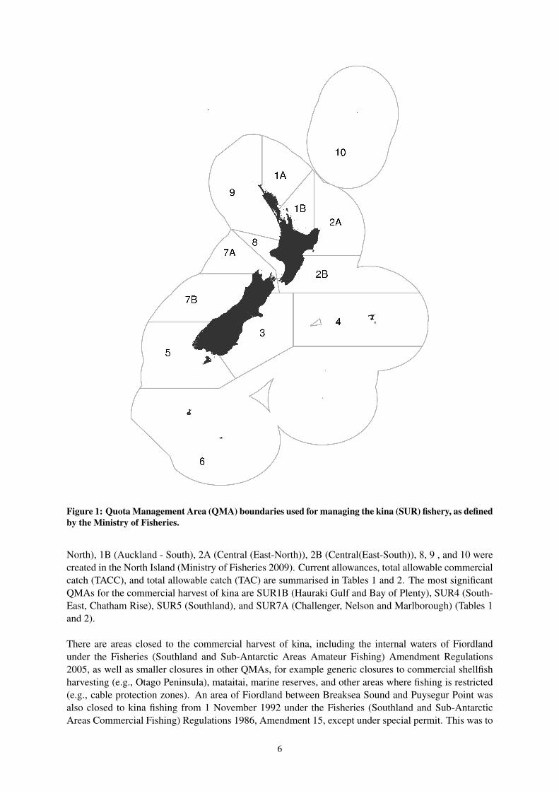
Figure 1: Quota Management Area (QMA) boundaries used for managing the kina (SUR) fishery, as definedby the Ministry of Fisheries.

North), 1B (Auckland - South), 2A (Central (East-North)), 2B (Central(East-South)), 8, 9 , and 10 werecreated in the North Island (Ministry of Fisheries 2009). Current allowances, total allowable commercialcatch (TACC), and total allowable catch (TAC) are summarised in Tables 1 and 2. The most significantQMAs for the commercial harvest of kina are SUR1B (Hauraki Gulf and Bay of Plenty), SUR4 (South-East, Chatham Rise), SUR5 (Southland), and SUR7A (Challenger, Nelson and Marlborough) (Tables 1and 2).

There are areas closed to the commercial harvest of kina, including the internal waters of Fiordlandunder the Fisheries (Southland and Sub-Antarctic Areas Amateur Fishing) Amendment Regulations2005, as well as smaller closures in other QMAs, for example generic closures to commercial shellfishharvesting (e.g., Otago Peninsula), mataitai, marine reserves, and other areas where fishing is restricted(e.g., cable protection zones). An area of Fiordland between Breaksea Sound and Puysegur Point wasalso closed to kina fishing from 1 November 1992 under the Fisheries (Southland and Sub-AntarcticAreas Commercial Fishing) Regulations 1986, Amendment 15, except under special permit. This was to

6

enable the kina fishery development programme, which arose from a proposal to commercially harvest1000 t of kina per year from Fiordland, to proceed. The project had two objectives: to gather informationon the biology of kina, along with estimates of sustainable harvest, and, to develop export markets forkina roe. A kina processing factory was set up by Uni Fishing Company Limited (a Taiwanese jointventure company), but the factory closed within a year of opening due to low export prices and poormarket acceptance (Guardians of Fiordland’s Fisheries 1999). The kina development programme wasdiscontinued in 1995 (Guardians of Fiordland’s Fisheries 1999) but the kina development programmearea remained closed to commercial kina fishing until November 2004 when the Fisheries (Southland andSub-Antarctic Areas Commercial Fishing) Amendment Regulations (No 2) 2004 revoked Regulation 15Fof the Fisheries (Southland and Sub-Antarctic Areas Commercial Fishing) Regulations 1986 to re-openthe area to fishing.

Table 1: Recreational and customary non-commercial allowances, TACCs and TACs (tonnes) for SouthIsland and the Chatham Islands kina fishstocks 3, 4, 5, and 7 for the 2008–09 fishing year

Fishstock Recreational Customary Other Mortality TACC (t) TAC (t)

SUR3 10 10 1 21 42SUR4 7 20 3 225 255SUR5 10 10 5 455 480SUR7A 20 80 3 135 238SUR7B 5 10 1 10 26

Table 2: Recreational and customary non-commercial allowances, TACCs and TACs (tonnes) for NorthIsland kina fishstocks 1A, 1B, 2A, 2B, 8, 9, and 10 for the 2008–09 fishing year

Fishstock Recreational Customary Other Mortality TACC (t) TAC (t)

SUR1A 65 65 2 40 172SUR1B 90 90 4 140 324SUR2A 60 60 4 80 204SUR2B 35 35 2 30 102SUR8 12 12 1 1 26SUR9 11 11 1 10 33SUR10 0 0 0 0 0

Kina are of high significance for Maori, but there is a paucity of data on landings occurring undercustomary fishing. Customary fishing is managed under two sets of regulations stemming from theTreaty of Waitangi (Fisheries Claims) Settlement Act 1992: the Fisheries (Kaimoana Customary Fishing)Regulations 1998, and the Fisheries (South Island Customary Fishing) Regulations 1999. These arehereafter referred to as the Kaimoana Regulations, and South Island Regulations, respectively. There is arequirement under these regulations for Tangata Kaitiaki / Tiaki (those who authorise customary fishing)to file quarterly returns to the Ministry of Fisheries, accurately detailing species and quantities takenunder customary fishing authorisations. However, until either the Kaimoana or South Island regulationsare implemented by tangata whenua in a particular place, regulation 27A of the Fisheries (AmateurFishing) Regulations 1986 (hereafter referred to as Regulation 27A) may be used by customary fishers.Fishers must be able to demonstrate that they are fishing for the purpose of a hui or tangi, and have beenauthorised to fish in accordance with the conditions in Regulation 27A. There is no mandatory reportingrequirement under Regulation 27A. The customary fishing regulations do not remove the right of tangata

7

whenua to take fish as recreational fishers.

There are few data on the recreational fishery for kina as there is no requirement to report landings.According to the Ministry of Fisheries, there is some illegal harvest of kina, but actual levels are notquantified (Ministry of Fisheries 2009).

There is currently no formal stock assessment of sustainable yield for kina, and no estimates of biomassor trends in abundance for any fishstock (Ministry of Fisheries 2009). However, there is some informationon densities (e.g., Schiel et al. 1995), indices of relative abundance (e.g., Naylor & Andrew 2002), andbiomass (see McShane & Naylor 1991, McShane et al. 1993, and McShane et al. 1994). There is noestimate of maximum constant yield (MCY) for any kina fishstock although Annala (1995) reported anestimate of MCY for kina in Dusky Sound and Chalky Inlet. It is not known if kina fishstocks are at levelsallowing the stocks to move towards a size that will support sustainable yields, and the sustainability ofcurrent catch levels or TACCs is also unknown for kina fishstocks(Ministry of Fisheries 2009).

2. METHODS

2.1 Literature review

Relevant literature on urchin and other sedentary invertebrate fisheries was reviewed, with a focus onkina biology and ecology, management of invertebrate and urchin fisheries, information requirementsfor the sustainable management of invertebrate fisheries, and stock assessment of urchin fisheries.

2.2 Fisher interviews

Semi-structured interviews, whereby a set of questions guides the interview process to gather in-depthinformation, but the interview is flexible and conversational in structure (Lindlof & Taylor 2002), werecarried out with 27 commercial and customary fishers in the four key quota management areas (SUR1B,4, 5, and 7A) to capture issues unique to each QMA and to assist with interpreting patterns in thecatch effort data. The questionnaire used as the basis for the semi-structured fisher interviews is givenin Appendix A. Those commercial fishers with the highest catches in each QMA were identified aspotential interview participants, with the assistance of Ministry of Fisheries compliance and policy staff.Contact details for kina fishers were obtained from FishServe. Pou Takawaenga and Pou Hononga,along with Te Runanga o Ngai Tahu (for SUR5), assisted with the identification and contact details forcustomary fishery interview participants. Interview questions included topics such as harvesting strategy,kina size and roe quality, monitoring and reporting, market, and value. Interviewees were asked beforethe interview whether the interviewer could take notes. They were also asked if the interview could berecorded (except where the interview was conducted by phone). A voice recorder was used to recordthe interview where permission was given by the interviewees. These recordings were to assist withtranscription and have not been made available to the Ministry of Fisheries.

All participants were provided with an information sheet summarising the kina characterisation project,either before being interviewed or at the interview. Following each set of interviews, largely uneditedinterview notes were returned to all interview participants with a cover letter or email that askedparticipants to check the notes and confirm whether they were comfortable with the information theyprovided being used. Permission was also sought from one of the interviewees to include transcripts ofhis interview notes in Appendix B.

A summary of interview participants is presented in Table 3. In SUR7A, all the active fishers interviewed

8

dived for kina, except one who been involved in the dredge fishery. In SUR4, both iwi representativesfrom the Customary Fishing Forum on the Chatham Islands were met, although only one representativewas interviewed. The ex-fisher interviewed in SUR5, although not a Kaitiaki, represented customaryfishing interests and was interviewed at the same time as the two SUR5 Kaitiaki. Although all threeSUR5 customary fishing interviewees were interviewed in a small group, the responses provided byindividuals did not appear to be influenced by the presence of the other interviewees. The key opinionsand comments for commercial and customary fishers are summarised in the results section.

Table 3: Summary of customary and commercial fishers interviewed in QMAs SUR1B, SUR4, SUR5, andSUR7A. Each of the 27 individual interview participants are represented as a single horizontal category,with bullets denoting the category (or categories) within which each participant fits (e.g., the first line isa commercially active fisher and processor, whereas the second line is an ex-commercial fisher, who is aKaitiaki and customary fisher). The category ex-fisher refers to commercial fishers who have fished kinapreviously but are no longer active commercial kina fishers. Note that eight interview participants fittedmore than one fisher category. The total number of categories encompassed by all interview participants issummarised at the bottom of the table.

Area Commercial Customary

Active fisher Processor Ex- fisher Kaitiaki Fisher

SUR1B • • - - -- - • • •- - • - -- - - • •- - - • •

SUR4 • - - - •• - - - -- • - - -- • - - -- • - - -- - • - -- - • - -- - - • -

SUR5 - • • - -• • - - -• - - - -- - - • -- - - • -- - • - -

SUR7A • - - - -• - - - -• - - - -• - - - -• - - - -- - - - •• • - - •• • - - •

TOTAL 12 8 6 6 7

9

2.3 Commercial catch effort data

All commercial fishing activity for kina is reported to the Ministry of Fisheries and entered into the catcheffort database. An extract from the catch effort database was obtained, with all fishing event catch andlanding data from trips that had either

1. landed SUR,

2. caught SUR (either target or non-target),

3. targeted GUR or KIN with a primary method of DI (Diving) or H (Hand gathering).

The third rule was needed as some SUR catch has been recorded as GUR (due to data entry errors), orKIN (due to fishers using the KIN code in error). The New Zealand fishing year for kina runs from 1October to 30 September in the following year. Data were used from the 1989–90 to the 2008–09 fishingyears.

Tables and plots summarising each of the last 20 years of fishing were produced for catch and effortdata from each QMA, for each of the two fishing methods for kina (breath-hold dive and dredge)(seeAppendix C). The annual distribution of kina catch in each QMA was summarised by month andstatistical area in Appendix C.

Catch per unit effort for dive fisheries was calculated from the CELR data by using number of diversper day as the unit of effort (recorded on the CELR form as effort number). The time spent diving isalso recorded on the form; however this is not regarded as reliable due to some fishers recording the totaltime spent diving by all divers, and some fishers recording the duration of fishing (e.g., if four diversdived together for 6 hours, some fishers would record the time spent diving as 24 hours, and some wouldrecord it as 6 hours). For dredge fishing, CPUE was calculated by dividing the estimated greenweight bythe hours fished.

2.4 SUR5 Association fine-scale data

In the SUR5 QMA, the SUR5 Association Incorporated Society (SUR5 Association) was formed tomanage the interests of stakeholders (since July 2010, the SUR5 Association has transformed into anational body representing commercial kina fishers known as the Kina Industry Council (KIC)). At thestart of the 2004–05 fishing year, the SUR5 Association adopted a code of practice to actively managethe fishery to ensure sustainability and development. In addition to existing reporting via catch effortlanding returns, and monthly harvest returns, the code of practice requested that fishers report kina catchat a finer scale. Fine-scale monitoring was implemented in support of a proposal to partially re-openan area of SUR5 that had been closed to commercial kina fishing since the early 1990s as part of theexperimental kina development programme. Fishers record the harvest of kina using SUR Catch EffortLanding Return (SCELR) forms, where the fine-scale areas correspond to those used by paua fishers inPAU5A, B and D on the Paua Catch Effort Landing Return (PCELR) forms. An example of a completedform is given in Figure 2.

A single fisher from SUR5 has been maintaining voluntary fine-scale data collection since the 2004–05fishing year, giving the forms to the SUR5 Association. Monthly summaries of the fine-scale data arealso provided to the Ministry of Fisheries as total landed greenweight per fine-scale statistical area. Withthe permission of the fisher concerned, the SUR5 Association provided Dragonfly with the fine-scaledata for analysis.

10

Figure 2: A scanned copy of a completed SCELR form, used for collecting fine-scale kina catch effort datain SUR5. The form is reproduced at 50% of actual size, with identifying names and numbers obscured.

Copies of paper fine-scale forms were obtained from the SUR5 Association, for the period from thebeginning of the 2005–06 fishing year through to the end of the 2008–09 fishing year. The forms followedthe format of the PCELR forms, with a form being completed for each day’s diving. For each diver,the form has a record of the paua statistical area, the time spent in the water (hours and minutes), theestimated catch of kina (kg), and a record of the diving conditions with the codes P (Poor), A (Average),G (Good), and E (Excellent). In addition, the forms contain information on the landings, details of thepermit holder, and the name of the fishing vessel. On many forms the depth of the diving (in feet) wasrecorded. All data from the forms were double entered into a purpose-built database, with data entryerrors being checked by reconciliation against the original paper forms.

From the entered data, a catch per unit effort (CPUE) was derived for each individual diver record bydividing the catch by the time spent in the water. Relationships between the CPUE and the other datarecorded on the PCELR forms were explored graphically.

To determine whether there had been changes in the CPUE over the period of the data, mixed-effectslinear-models were fitted to the data. Two models were fitted, one to all the fine scale data from the SUR5

11

QMA, and one that was restricted to data from the area that had the most fishing effort. Restricting themodel to a single area allowed changes in CPUE to be investigated with a reduced possibility that serialdepletion would be masking any changes in kina CPUE.

The logarithm of the CPUE of a daily diver record, indexed by i, was estimated as a linear function of Ncovariates x, an intercept β0, and error terms, λ , λa, and λ f ,

log(CPUE) = β0 +N

∑j=1

β jxi j +λi +λ fi +λai . (1)

The intercept, β0 and the coefficients of the covariates β j were estimated during model fitting. Therewere three error terms, one term that was different for each record (λi), one term that was the same for allrecords on the same form (λ f ), and one term that was the same for all records in the same area (λa). Thestructure of these random effects allows for correlation between records from the same paua statisticalarea, and for records from the same form. The errors are obtained by sampling from respective normaldistributions,

λi ∼ Normal(0,σ), (2)

λ f ∼ Normal(0,σ f ), (3)

λa ∼ Normal(0,σa). (4)

The model parameters were fitted using Bayesian methods, by Gibbs sampling. The model was written inthe BUGS modelling language (Spiegelhalter et al. 2003), using the software JAGS (Plummer 2005). Themodels were run for 10 000 updates during burn-in, and then run for a further 50 000 updates, with every10th sample being retained for analysis. During model fitting, estimates were made for the parameters β0,β j, σ , σ f , and σa, using two independent Monte-Carlo Markov chains. Model convergence was checkedby using tests from the CODA library (Plummer et al. 2006).

Bayesian modelling requires prior distributions for unknown parameters. Diffuse normal priors wereused for the β coefficients, a diffuse Gamma prior was used for the standard deviation σ , and a half-Cauchy prior was used for the standard deviations σa and σ f (Gelman 2006),

β0 ∼ Normal(µ = 0,σ = 100), (5)

β j ∼ Normal(µ = 0,σ = 100), (6)

σ ∼ Gamma(scale = 1000,shape = 0.001), (7)

σ f ∼ Half-Cauchy(scale = 200), (8)

σa ∼ Half-Cauchy(scale = 200). (9)

A key step in the model fitting was the selection of covariates. The potential covariates listed in Table 4were tested for inclusion in the model by using an simpler model (without the random effects λ f or λa),fitted with maximum likelihood techniques. An automated step analysis was used that tried potentialcovariates in turn, retaining the covariate that caused the greatest reduction in the Akaike InformationCriterion (AIC) (Akaike 1974). The process was repeated until there was no further reduction in the AICby adding further covariates. The selected covariates were then included in the full Bayesian model.

2.5 Customary harvest data

Under the Kaimoana Regulations and the South Island Regulations, Tangata Tiaki / Kaitiaki are requiredto file quarterly returns to the Ministry of Fisheries accurately detailing species and quantities taken

12

Table 4: Potential covariates tested for inclusion in the models of catch per unit effort.

Covariate Values Description

Fishing year 2005–06 to 2008–09 The fishing year, included as independent factors.Diver Diver number An identifier for each diver, based on the diver name

recorded on the PCELR forms. There were seven diverswho had recorded more than 20 days of fishing, and theywere included individually. The remainder were groupedtogether.

Condition P, A, G, E Summary of diving conditions, as recorded on thePCELR forms. The codes are P (Poor), A (Average), G(Good) and E (Excellent). During grooming, codes ofVG were set to E, and codes of VP or V were set to P.

Depth 5 to 30 Depth of diving, recorded as additional information forover 95% of records.

Region F, S Area classified as Fiordland (F) or Stewart Island (S),based on the letter of the paua statistical area code.

Hours 0.5 to 10 Time underwater, converted from hours and minutes todecimal hours.

Cosine yearday -1 to 1 The cosine of the day of year, y, calculated ascos(2πy/365).

Sine yearday -1 to 1 The sine of the day of year, y, calculated as sin(2πy/365).

under customary fishing authorisations. If neither the Kaimoana or South Island Regulations havebeen implemented by tangata whenua in a particular place, customary fishing may take place underregulation 27A of the Fisheries (Amateur Fishing) Regulations 1986. Unlike the Kaimoana or SouthIsland Regulations, reporting is not mandatory under Regulation 27A, and consequently data are notreported for all customary fishing events.

Customary data furnished as quarterly returns are held in a database under contract to the Ministry ofFisheries. Pou Hononga, who manage the contract for the customary database, permitted the release ofthe customary data to Dragonfly. Data were provided as an Excel spreadsheet and detailed the regulationsthe data was reported under, year, quarter, report provider (i.e., the hapu, marae, trust, or iwi providingthe report), the quantity and unit type approved for harvest (bag, bin, weight in kilogrammes, number,sack, sugar sack), the actual quantity and unit type harvested, fisheries management area, and fishstockcode.

There were many records with missing unit types. The following rules were used to complete the unittype data:

• If the unit type was provided for the approved harvest, but not the actual harvest, then the unit ofthe actual harvest was assumed to be the same as for the approved harvest.

• The largest actual harvest with a unit type of kilogrammes was 3440, any harvests larger than thiswere assumed to be numbers of kina.

• If reporting by an entity (e.g., a hapu) was always in one unit (e.g., sacks), then all harvests withmissing units reported by that entity was also assumed to have that unit.

From the reported harvest, a harvest in kilogrammes was then derived. Numbers of kina were convertedto kilogrammes by following the method of Ministry of Fisheries (2009), and assuming that the averageweight of a harvested kina was 0.2483 kg. According to one of the customary fishers interviewed, astandard sack of kina converts to between 35 and 50 kina (dependent on kina size). In a guide for

13

Kaitiaki, the company e-Fish suggest that a bin of kina weighs 30 kg. We assumed that the bulk units(sacks, bins, bags, sugar sacks) all weighed 25 kg. Reported harvest that had no unit was not included insummaries or aggregates.

3. RESULTS

3.1 Literature review

3.1.1 Kina ecology

Kina (Evechinus chloroticus) are distributed along the coast of mainland New Zealand and are also foundin the subantarctic and Chatham Islands (Fell 1960, Pawson 1961, Dix 1970a). In northern New Zealand,dense populations of kina are found on shallow rocky reefs dominated by encrusting algae (Barker 2001).They generally occur at depths less than 12 to 14 m (Andrew & Choat 1985, Shears & Babcock 2007)but can be found at depths up to 60 m. In the north of the North Island kina commonly form barrens,which are areas with low algal abundance and dense aggregations of kina (McShane & Naylor 1991). Inthe South Island, kina commonly form aggregations, either between single kelp plants or small groupsof kelp, or form small barrens areas (5 to 6 m2), but not to the extent of barrens observed in the northof the North Island (Barker 2001). Shears & Babcock (2007) noted that in southern New Zealand,kina are rarely found in highly exposed areas such as the West Coast, unlike northeastern areas of NewZealand where there is a positive association between exposure and density. Kina are more common onthe southern coasts and very common around Stewart Island. However, along the Otago coast, kina areuncommon, being found in isolated aggregations, possibly as a result of sporadic recruitment (Barker2001). In the Chatham Islands, kina are abundant where Carpophyllum flexuosum is common, andextensive kina barrens are not observed (Schiel et al. 1995). Kina are seldom found on fine sedimentslike silt or mud (Barker 2001, Shears 2007).

Kina occur in variable densities around New Zealand. In northern New Zealand, kina can reach densitiesof up to 40 m−2 (Choat & Schiel 1982). In Fiordland, kina can reach similar densities (20 to 30 m−2), andare found just below the low salinity layer that occurs in the fiords (McShane & Naylor 1991, Wing etal. 2001). Kina densities differ between the inner fiords and the fiord entrances with average densities of5.22 m−2 at the entrance to Doubtful Sound, and 1.81 m−2 at Deep Cove at the head of Doubtful Sound.In a survey of kina in Fiordland, average kina densities ranged between 1.1 and 3.0 m−2, with numbersalways higher in water less than 9 m deep (McShane & Naylor 1991). Less than 10% of all kina surveyedwere in water deeper than 9 m (McShane et al. 1993). Relatively high kina abundances were recordedby Shears & Babcock (2007) in Paterson Inlet (Stewart Island) and Preservation Inlet (Fiordland), withvariable kina densities at exposed coastal locations where dense aggregations were only found at depthsgreater than 10 m. Very few kina juveniles were recorded at open coast sites where kina were in denseaggregations in deeper water, with Shears (2010) suggesting these populations are probably recruitmentlimited and therefore vulnerable to commercial kina fishing.

Spawning in kina is spatially and temporally variable (Brewin et al. 2000) occurring between Novemberand March (Dix 1970a, 1970b, McShane et al. 1994a, Lamare 1998, Anderson & Millar 2004). Althoughthe degree of spatial and temporal variability in spawning is difficult to quantify, Lamare and Stewart’s(1998) observation of a spawning event in Fiordland suggested that the spatial scale of spawning maybe as large as 40 km (Lamare & Stewart 1998). The larval duration of kina in the water column is 20 to40 days before settlement (Lamare & Barker 1999, Walker 1984). Settlement is spatially variable, withkina populations often comprised of single cohorts (Dix 1970a, 1972). There is some evidence fromFiordland for the coupling of settlement and recruitment (Lamare & Barker 2001). However, this may bedue to characteristics of the fiord system that are not found elsewhere in New Zealand (Lamare & Barker

14

2001). Keys (2008) found that spawning activity in kina varied between two size classes of kina (over140 mm and 80 to 100 mm test diameter), and sites (Foveaux Strait coast and southwest Fiordland). Atboth sites, gametogenesis started in midwinter, but mature gametes were observed at the Foveaux Straitsite between August and January, and at the southwest Fiordland site between October and February(Keys 2008). Spawning in small urchins at the southwest Fiordland site took place between October andDecember, and larger urchins spawned between December and February (Keys 2008).

Kina reach ages between 10 and 20 years (Dix 1972, Lamare & Mladenov 2000, Barker 2001), with sizeat maturity and growth varying between locations (Dix 1970a, 1972, McShane & Naylor 1991, Barkeret al. 1998, Wing et al. 2003). Dix (1972) used growth bands in the test of kina to estimate age, butthis method has not been validated (Andrew 2000). The red sea urchin, which is found along the westcoast of North America, was reported as having a lifespan of 7 to 10 years by Sloan (1986), but this wasradically revised by Ebert (1996), Ebert et al. (1999), and Ebert & Southon (2003), to suggest that largered sea urchins reached over 100 years of age. Ebert & Southon (2003) attributed the long life of adultred sea urchins to a requirement for many annual reproductive cycles to successfully produce offspringthat settle and survive to reproductive age. This life-history strategy led Ebert & Southon (2003) tosuggest that large individuals of other long-lived sea urchins, such as Evechinus chloroticus, need to beprotected.

Juvenile kina (less than 40 to 50 mm test diameter) tend to be cryptic, living in crevices and under rocksbefore moving to more open habitats once they recruit into the adult population (Dix 1970a, Shears& Babcock 2002). In Fiordland, size at first maturity occurred at about 50 mm test diameter (TD)(McShane & Naylor 1991). Size at maturity of kina populations is spatially variable. Dix (1970b)looked at maturity of kina populations at sampling locations at Kaikoura and Kaiteriteri. Size at firstmaturity for kina at Kaiteriteri occurred between 35 mm and 45 mm test diameter (TD), and for kina fromKaikoura, between 55 mm and 75 mm TD. Although size at first maturity differed between Kaikouraand Kaiteriteri populations, kina were the same age at first maturity (3–4 years at both Kaiteriteri andKaikoura). Studies from overseas on other echinoderms suggest these differences in maturity betweenlocations may be food related. Kawamura (1964) found maturity in Strongylocentrotus intermedius inJapan could be reached in a year where food is plentiful but 1 to 2 year old urchins may still be immaturewhen food is limited, while, in the United Kingdom, Buchanan (1966) noted maturity could be deferredin the urchin Echinocardium cordatum.

Kina typically have a unimodal size distribution dominated by larger individuals (e.g., Otago (Barker2001), Kaikoura and Kaiteriteri (Dix 1972), Tory Channel (Lamare & Barker 2001), and Dusky Sound(McShane 1992)). Dix (1972) showed that size structure can be quite distinct over distances of less than5 km. Wing (2009) found strong temporal and spatial variability in the size structure of kina at 22 studysites in Fiordland, and suggested that the effect of the availability of high-quality food on adult growthand survivorship, and the effect of estuarine circulation on recruitment, influence the size-structure ofkina in this region.

Lamare (1997) used a model presented by Ebert (1973), based on the analysis of population sizestructure, to calculate instantaneous mortality. He calculated annual mortality and mean longevity ofkina to be 9.21% and 10.38 years for Doubtful Sound, and 5.01% and 19.33 years, respectively, forTory Channel. Mortality can result from predation by large starfish, benthic feeding fishes, lobsters, andmolluscs (Lamare 1997); periodic fluxes in salinity, particularly for juvenile kina in Doubtful Sound(Barker 2001); human predation via fishing; and disease (Lamare 1997). Phillips & Shima (2006)demonstrated that larval mortality rates of kina increased with increasing concentrations of suspendedsediment. Similarly, Walker (2007) also demonstrated that the presence of fine sediments inhibitedkina larval settlement, and decreased the survival of recruits and juveniles. This suggests there may benegative impacts of run-off from the land on kina populations (Morrison et al. 2009).

15

Kina are primarily herbivorous but have been shown to eat a range of food if the availability of algae islimited (Dix 1970a). A field exclusion experiment by Andrew & Choat (1982) demonstrated the influenceof kina on kelp stands, with the exclusion of kina resulting in increases in kelp biomass across a 1000 m2

coralline flat. Ayling (1978) also demonstrated the role of kina in structuring encrusting communities,with kina shown to graze on all but the more massive sponges. In Fiordland, more food was found inthe gut of kina from the entrance to the fiords where laminarian kelp dominated by Ecklonia radiata arefound, than in kina at the inner fiords, where nutrition is thought to be limited by only red algae andfilamentous green algae (Wing et al. 2001).

Importantly, urchins can play a key role in structuring marine communities (Lawrence & Sammarco1982, Sammarco 1982). Major changes in community structure can occur, as exemplified in theCaribbean when intense fishing of urchin predators led to a single species of urchin subsequentlydominating the herbivorous community (Lessios 1988, Jennings & Polunin 1996). In New Zealand,numerous studies have examined the role kina play in subtidal communities (Schiel 1982, Andrew 1988,Andrew & MacDiarmid 1991, Schiel et al. 1995, Cole & Keuskamp 1998, Cole 1999, Anderson & Millar2004, Parsons et al. 2004, Salomon et al. 2008, Jack et al. 2009), with much of this work specificallyfocused on marine reserve effects (Babcock et al. 1999, Shears & Babcock 2002, 2003, Shears et al.2008).

Shears & Babcock (2003) concluded that when the numbers of predatory fish and lobster increasedfollowing the formation of the Leigh Marine Reserve, a subsequent decrease in the kina population led tothe growth of macroalgae. Villouta (2000) found when kina densities dropped below 2 m−2, the densityof Ecklonia radiata increased markedly. A similar relationship was demonstrated for Carpophyllum spp.when kina densities dropped below 3 m−2. Urchins are able to maintain dense aggregations in barrenshabitats by making use of energy reserves stored in gonad tissue (Giese 1967). When urchins are starved,movement has been shown to be greater than in those that are not (Hart & Chia 1990), but others havefound no effect of starvation on movement (Klinger & Lawrence 1985, Dumont et al. 2004). Mattison etal. (1976) showed that urchins in kelp forests move less (7.5 cm day−1) than urchins outside kelp forests(50 cm day−1). The increased movement of urchins outside of the kelp forest may result in the format ofurchin feeding fronts (Abraham 2007), dense aggregations of urchins grazing at the boundary betweenthe barrens and kelp habitat. Villouta et al. (2001) warned that the strong influence of urchins on subtidalcommunities needs to be considered in the development of urchin fisheries, with large scale commercialurchin fisheries likely to have impacts on ecosystems that need to be managed (Tegner & Dayton 2000).

There are other examples of trophic interactions between kina, their predators, and macroalgae (e.g.,Estes et al. 1998), but processes such as disease and broader oceanographic events are also importantin structuring subtidal assemblages (e.g., Sala et al. 1998). In a review of the environmental effectsof fishing for rock lobster (Jasus edwardsii), Breen (2005) concluded that the evidence for an urchin-mediated effect of lobster fishing on the algal assemblage was weak, largely due to the complexityof the relevant ecological interactions. Shears et al. (2008) compared kina abundance, the extent ofurchin barrens habitat, and macroalgal biomass between reserve and fished sites at six locations acrossa range of environmental gradients. In their examination of whether fishing or environmental factorsdescribed variation among sites, they found that environmental variables could explain variation betweenreserve and fished sites equally as well as fishing. They suggest the role kina play in controllingmacroalgal biomass varies at local and regional scales relative to abiotic factors such as sedimentationand wave exposure. Consequently, it is difficult to predict the ecosystem effects of fishing without betterunderstanding of the effect of environmental variation on species interactions at multiple spatial scales(Shears et al. 2008).

There is evidence from New Zealand and overseas that suggests urchins can limit abalone populations(Andrew et al. 1998, Naylor & Gerring 2001, Konstantin et al. 2001). Konstantin et al. (2001) found an

16

inverse correlation between red sea urchins (Strongylocentrotus francsicanus) and red abalone (Haliotisrufescens) abundance in northern California. In New South Wales, Andrew et al. (1998) demonstrateda negative relationship between the spiny sea urchin (Centrostephanus rodgersii) and the commerciallyimportant red abalone (Haliotis rubra). In New Zealand, Naylor & Gerring (2001) also demonstratedan inverse relationship between kina and paua (Haliotis iris) densities where increased kina densitiesresulted in decreased paua densities. In contrast, a positive correlation has been shown betweensome species of juvenile abalone and adult urchins, with adult urchins providing juvenile abalone withprotection from predation (Mayfield & Branch 2000).

Body size and gamete production have been shown to be directly proportional across a range oftaxa (Paris & Pitelka 1962, Rinkevich & Loya 1979, Suchanek 1981). This has implications forfisheries management as harvesting of large individuals would have a disproportionate effect on gameteproduction. However, Levitan (1991) warn that large body size and high gamete production does notnecessarily confer reproductive success if the value of fertilisation success is not taken into account.Work by Levitan et al. (1992) in British Columbia on the red sea urchin (Strongylocentrotus franciscanus)has demonstrated that increased group size and aggregation, a central or downstream location within anaggregation, and decreased current flow all increase fertilisation success. The resulting implication forkina fisheries is that even if a number of larger fecund individuals are not harvested, they need to be atdensities that will allow them to successfully reproduce. Further, the potential dependence of recruitson protective adults, in combination with allee effects (where there is a positive relationship betweenreproductive success and density (Stephens et al. 1999)), makes urchins prone to fishing reducing thestrength of recruitment (Pfister & Bradbury 1996). However, Mead (1997) found that unlike many urchinspecies elsewhere in the world, kina seem capable of achieving high rates of fertilisation success overseparation distances as high as 6 m. They calculated the minimum adult densities to achieve this successwere between 0.33 and 0.67 m−2.

In urchin fisheries, there can be a preference to remove mainly smaller, mature individuals as the financialreturn is determined by roe quality rather than absolute size or weight (Jamieson et al. 1998). This canlead to newly mature urchins being exploited over older, larger urchins that may have poor roe quality,which, in turn, can create a large adult refuge, unless fishers deliberately destroy these larger urchins toincrease available food to younger urchins (Jamieson et al. 1998). How fishing affects the populationdepends on the rate of exploitation and the proportion of the population that makes it into the adultrefuge, which, if fishing is intense, can be small (Jamieson et al. 1998). Size selective harvesting mayregulate the biomass and production of fished urchin populations, with urchins in areas closed to fishingable to reach greater sizes, and therefore having higher productive potential (Nick Shears, University ofAuckland, pers. comm.). Currently, as there is no size limit in the kina fishery in New Zealand, androe quality not being a driver for most fishers, the preference observed in other urchin fisheries for theremoval of smaller urchins may be less relevant to the kina fishery in New Zealand. However, shouldinternational markets for kina be developed in future, where smaller kina are more desirable due to theircolour and roe quality, then the size of harvested kina will become an important consideration in themanagement of the fishery.

Kritzer & Sale (2004) described a metapopulation as “a system of discrete local populations, each ofwhich determines its own internal dynamics to a large extent, but with a degree of identifiable andnon-trivial demographic influence from other local populations through dispersal of individuals.” Sincethe mid 1990s, the inclusion of metapopulation ecology in fisheries science has increased (Stephenson1999). Wing (2009), in relation to kina, cautioned that the implication of fishing source populations onthe metapopulation needs to be considered, along with the implications of fishing isolated populationsthat are self-recruiting e.g., geographically isolated kina population in Long Sound, Fiordland.

For urchins in general, the size of the gonad relative to test size is commonly used as an index of

17

nutritional state (Harrold & Reed 1985), with the quality and quantity of food eaten by urchins alsoknown to influence the colour of urchin roe (Mottet 1976, Tegner 1989). Studies by Andrew (1986)and Choat & Andrew (1986) on kina, and Tegner (1989) and Harrold & Pearse (1987) on other urchinspecies, found a negative relationship between kina density and gonad indices. However, in their surveysin Fiordland, McShane & Naylor (1991) did not find a negative relationship between density and gonadindices suggesting the lack of relationship was due to high food availability in Dusky Sound and ChalkyInlet. In large kina (over 150 mm TD), McShane & Naylor (1991) suggested that the small size ofgonads relative to body size indicates that maintaining large body mass may limit available energy forreproduction.

The harvest of kina by freedivers results in minimal habitat damage. However, dredging is non-selective,with the potential impacts of dredging including damage to habitat caused by the dredge dragging acrossthe substratum, the non-selective removal of bycatch, and dislodgement or damage to fauna on or nearthe surface attracting increased predators to the area dredged (Currie & Parry 1994, 1999, Thrush et al.1998, Cranfield et al. 2003, Kaiser et al. 2006).

3.1.2 Fisheries specific kina research

There is little information on the size of kina populations around New Zealand with few fisheryindependent assessments of kina stock status. Data predominantly collected by university researchersand crown research institutes include densities (e.g., Schiel et al. 1995) and indices of relative abundance(e.g., Naylor & Andrew 2002, Ministry of Fisheries 2009). There are also estimates of biomass forChalky Inlet of 260 t (95% c.i.: 154 to 366) and Dusky Sound of 3401 t (95% c.i.: 2593 to 4209) inFiordland (see McShane & Naylor 1991), and D’Urville Island (2500 t) and Arapawa Island (500 t) inthe Marlborough Sounds (see McShane & Naylor 1993).

McShane & Naylor (1991) gathered information on the population structure, morphometrics, andestimated biomass for kina in Dusky Sound and Chalky Inlet to provide baseline information for anexperimental kina fishery in Fiordland. In 1993, McShane et al. (1993) carried out surveys in DuskySound to investigate the effects of lowered kina densities by fishing on the sublittoral algal assemblages.They found a strong relationship between “jaw” length and test diameter and predicted that, withfishing, kina densities would decrease, growth of remaining kina would increase, there would be adecrease in relative jaw length, and an increase in relative gonad yield (McShane et al. 1993). Theyalso predicted that the floral composition of fished habitat would change, with decreased cover ofcrustose coralline algae, and increased density and canopy cover of Ecklonia radiata and Carpophyllumflexuosum. However, they were unable to test their predictions as the 133 t of kina harvested under theKina Development Programme was insufficient to cause a measurable change in kina density or seaweedcomposition (McShane et al. 1994a).

The kina fishery in New Zealand relies on obtaining good roe recovery. Research to improve roe recoveryinvolving translocation trials has been carried out in New Zealand, moving kina from areas where theirgonad index (GI) values were typically low, to areas where, historically, kina had very high GI valuesdue to an abundant food supply (James & Herbert 2009). After seven months, the GI of kina moved totranslocation sites had increased significantly relative to pre-translocation GI values. Surprisingly, therewere significantly greater increases in the GI of kina at the initial sites than at translocation sites (James& Herbert 2009). The researchers attributed this to reducing kina density, and the re-growth of algalspecies at the intial sites. The increases in GI from the translocation trial were of economic significanceas they could increase roe yield of kina by 50 to 100% (James & Herbert 2009). The results from thestudy by James & Herbert (2009) correspond with the suggestion by McShane & Naylor (1991) that kinaleft behind in lower densities post-fishing would have high growth rates due to the increased abundance

18

of seaweed available as food.

Roe enhancement trials have also been carried out on kina held in sea-cages and land-based tanks, andfed on artificial diets (James 2006). Both urchin roe quantity (GI) and quality (colour) were enhanced ina 12 week period using an artificial diet (James 2006).

The difficulty in providing suitable kina roe for the international market has driven research on dietsfor kina that could improve roe quality (Barker et al. 1998, Buisson & Barker 2001, Fell & Barker2001, James et al. 2007, 2009, James & Heath 2008, Phillips et al. 2009). The improvement of roequality, especially colour and taste, via enhancement programmes for wild harvest kina, would assistwith development of an export fishery.

Researchers based at the University of Otago have developed a method to objectively assess the sensoryqualities (i.e., appearance, odour, taste, flavour, texture, and aftertaste) of sea urchin roe (Phillips et al.2009). Phillips et al. (2010) investigated the sensory quality of kina roe from seasonal samples collectedover a two year period, relative to the sensory requirements of overseas markets for low bitterness andsweet taste. Previous research has demonstrated there are differences in taste between male and femaleurchins (Lee & Haard 1982, Murata et al. 1998, 2002). Phillips et al. (2010) also found differences intaste between male and female urchins, and found the sensory quality of female roe was closest to themore desirable sensory quality of male roe during autumn and winter. Phillips et al. (2010) advisedfurther research on kina diet be carried out to either alter the sensory quality of kina roe in spring andsummer when the GI is greatest, or use additional feeding to increase the GI of kina in autumn and winterwhen taste is best but GI is lowest.

Phillips et al. (2009) demonstrated that sex, season, and sexual maturity all contributed to differencesin the sensory properties of Evechinus chloroticus roe, with sex having the largest influence on sensoryproperties. They also found that larger male kina had darker coloured roe. This was consistent withprevious studies by McShane et al. (1996) and Woods et al. (2008), who found that smaller kina hadbetter roe colour (yellow or orange) than larger kina that had darkly coloured roe (brown or black).

James et al. (2007) investigated key holding and environmental conditions required to enhance the roe ofEvechinus chloroticus to better utilise the fishery resource. They found roe growth increased with greaterwater movement, probably due to increased dissolved oxygen and better removal of waste products fromaround the kina. The optimal period for roe enhancement, to achieve the maximum GI increase in theshortest period possible, was found to be between 9 and 12 weeks. Food availability was the primaryfactor associated with roe enhancement, followed by sea temperature. Significantly greater increases inGI occured in kina with low intial GIs than in kina with high initial GIs.

3.2 Review of relevant literature on urchin and other sedentary invertebrate fisheries

3.2.1 Sedentary invertebrate fisheries

S-fisheries are small-scale spatially structured fisheries targeting sedentary species (Orensanz et al.2005). Small-scale variations in the life-history traits of sedentary invertebrates can result in very smallfish stock units, ranging from dozens to hundreds of individual stocks in a fishery (Caddy 1975, Prince2005, Orensanz et al. 2005). Approaches to fisheries management where the unit stock in a fishery isidentified and fishing mortality is controlled to reach the maximum sustainable yield (Beverton & Holt1957) have long been recognised as inappropriate for sedentary invertebrates (Orensanz & Jamieson1998). Due to the high spatial structuring of sedentary invertebrate populations, the identification ofappropriate spatial scales for management is required (Caddy 1975, Orensanz et al. 2005, Schroeter

19

et al. 2009). The less mobile a species during any particular stage of its life-history, the greater theneed for spatially complex biological information (Caddy 1975). According to Prince (2003), the scaleof functional fishery management units in a fishery is best indicated by normal distances moved byindividuals within one or two seasons.

Monitoring and management of, often numerous, small-scale invertebrate stocks, particularly via typicalfishery-independent surveys involving diver counts along transects, is often well beyond the capacity ofmanagement authorities (Kalvass et al. 1991, Kalvass & Hendrix 1997, Parnell et al. 2006), with costsprohibitive particularly if the fishery is of relatively low value. As a result, in some fisheries this has ledto cooperative data collection between fishers and management agencies (Starr & Vignaux 1997), andthe use of commercial fishers to collect data (Prince 2003, 2005).

“Although fishery independent surveys could service this need for information, the spatialscale of most fisheries, combined with the patchiness of the resource, would mean that thecost of such surveys would be prohibitively high.” (Harrington et al. 2008)

Orensanz et al. (2005) summarised key elements necessary for the sustainability of S-fisheries, andsuggested that the difficulty in the sustainable management of such fisheries relates to incentives offeredby the management system not encouraging fishery participants (fishers, managers, scientists, and otherstakeholders) to behave responsibly. Orensanz et al. (2005) suggested that a first step towards incentivesfor responsible fisher behaviour are limited entry, clear entry rules, and monitoring of all effort, allimplemented with participation of fishers.

Overseas experiences (Harrington et al. 2008) have demonstrated that involvement of fishers ininformation collection, and increased involvement in management, helps develop leaders in the fishery,as well as the cooperation needed for the collection of fishery-dependent information for management.Harrington et al. (2008) outlined several advantages that industry-based surveys provide for spatiallymanaged fisheries, which included the potential to increase the value and economic return of fish andfish products.

Industry-based survey data are now incorporated into the spatial management framework of theTasmanian scallop fishery. Information collected includes fine-scale data (collected using GPS and dataloggers) to better understand the distribution of effort (Harrington et al. 2008). In 2003, the FisheriesResearch and Development Corporation (Australian government) investigated management rules forscallops and concluded the optimal spatial management regime for scallops was to have most scallopbeds closed with only a few open each year (Haddon et al. 2006). Harrington et al. (2008), in theircase study of the scallop fishery in Tasmania, stated that a combination of spatial management andimproved compliance helped with the development of rotational fishing regimes and paddock fishing,but information on stock status across the whole fishery was still required to decide which paddocks toclose and which to open. For scallops, at the least, managers need to know about size, condition, andrelative abundance in all available beds. The potential for industry-initiated spatial surveys to providethis information has been demonstrated (Haddon et al. 2006).

GPS technology has been used to accurately pinpoint the spatial location of abalone reefs in WesternAustralia’s commercial abalone fishery since the mid 1990s (Hart et al. 2009). GPS data are alsocollected in the South Australian abalone fishery. Shed sampling occurs in the New Zealand pauafishery where size information is collected to provide an estimate of the size frequency distributionof the commercial catch. Fine-scale recording of catch has been used since October 2001 in the pauafishery, with information incorporated into stock assessment models. An article in the September 2010issue of Seafood New Zealand describes the planned use of electronic data loggers by the paua industry

20

to capture information at a much finer scale than that currently gathered using the current paua statisticalreporting areas.

3.2.2 International urchin fisheries

Sea urchin fisheries generally have a poor sustainability record, with management in many urchinfisheries ad hoc or ineffective (Andrew 2000, Andrew et al. 2002). Andrew et al. (2002) and Andrew(2000) provided a detailed review of world sea urchin fisheries, describing a general boom and bustpattern of serial depletion at different locations, followed by declining stocks and, in some cases, collapse(Andrew et al. 2002, Williams 2002). According to Andrew & MacDiarmid (1999), a decade ago allmajor urchin fisheries, except those in Chile, were either in decline or had collapsed (e.g., France (Sloanet al. 1985), Ireland (Byrne 1990), California (Kalvass & Hendrix 1997), and Maine (Lesser & Walker1998)). However, the very high catches maintained in the Chilean fishery were explained by fishingmoving into new areas, rather than sustainable harvest of existing areas (Andrew & MacDiarmid 1999).

Andrew et al. (2002) noted there are likely a multitude of causes for world urchin fishery declines, thatare difficult to determine without stock assessments. Worldwide, very few urchin fisheries have hadstock assessments carried out, and, where assessment has occurred, surplus production methods havebeen used (Andrew et al. 2002). Surplus production models assume that catch-per-unit-effort (CPUE)may be used as an index of resource biomass, and by using a simple population model, the relationshipbetween CPUE and landed catch may be used to estimate a Maximum Sustainable Yield (MSY) for thefishery (e.g., Jennings et al. 2001). Surplus production models have the advantage that an estimate ofMSY may be made using only fisher-dependent data, with Perry et al. (2002) emphasising the utilityof detailed logbook information from fishers for input into the models. However, management advicearising from such stock assessments requires a precautionary approach, as the assumptions underlyingsurplus production models may not be correct. In particular, CPUE may not be a reliable index ofbiomass (e.g., Chen & Hunter 2003). Perry et al. (1999) also noted that techniques that rely on changesin catch rates may not be useful if there is not a sufficient decrease in catch rates in an area over time,which may be the case if fishing activity quickly moves to other locations.

Orensanz et al. (2005) presented a case study of the urchin fishery in Chile for a single species,Loxechinus albus. The fishery was open access with the only control being a 70 mm minimum size limit,but, due to sustainability concerns, particularly latitudinal serial depletion, it was placed under a quotaregime in 1999. Fisheries scientists estimated the total regional abundance of urchins using a size-basedmodel that had been previously applied to the predatory gastropod, loco (Conchelapas conchelapas).However, management of the fishery broke down in 2001 when there was conflict between fishers inadjacent fishing regions. This led to a programme where long-term fisheries management options wereexamined; the emphasis being on fishers, scientists, managers, industry associations, and federations ofartisanal fishers working together (Orensanz et al. 2005). Qualitative interviews were carried out withindustry managers, with the key findings being 1) the fishery operates by rotating areas spontaneously,and at different scales; and 2) there are large areas where the roe is too dark to be harvested. Thisinformation helped to develop a management strategy acceptable to fishers involving a formal rotationprogramme, tracking the recovery rate of harvested plots at a network of observation sites to fine-tunerotation times, the implementation of a legal harvest size, and the creation of reproductive refugeswhere roe colour makes the urchins unsuitable for harvest. In 2002, a formal management plan wasdeveloped by a technical advisory team, with all parties involved in the urchin fishery accepting theimplementation of a rotational experimental fishery. In summary, Orensanz et al. (2005) suggested thatthe main reason for fishery failures are not a lack of scientific knowledge but rather the application ofinadequate management structures.

21

The urchin fishery in Japan is also an exception to the overall boom and bust pattern in world urchinfisheries, having persisted for over 50 years under its current management regime based on exclusiveuser rights vested in fishing cooperatives, demonstrating the efficacy of management and the durabilityof the resource (Andrew et al. 2002). However, over the past 20 years, the fishery has exhibited apattern of longer-term declines in catch in spite of large-scale enhancement programmes (which aresubsidised by the government), fisheries closures, minimum legal sizes, and the current managementregime (Andrew et al. 2002). The long-term declines are predominantly due to decreased catches in theStrongylocentrotus intermedius fishery in Hokkaido and the S. nudus fishery in Miyagi, but accordingto Andrew et al. (2002), in the literature there are no formal assessments of stock status and there is alack of evidence demonstrating any restrictions of catch or effort, even in the face of declining catches, inJapanese urchin fisheries. Enhancement appears to be responsible for conserving and rebuilding Japaneseurchin fisheries (Andrew et al. 2002).

The decline in the Japanese fishery led to the development of new fisheries commencing on virgin stocksoff Chile, North America, and Australia that needed to deal with the issues of rising expectations duringa fishing-down phase and adjustment of the fishery for long-term sustainability (Williams 2002) i.e.,adjusting the level of effort after the initial fish-down stage to avoid exceeding the productive capacityof the fishery. Consequently, the fisheries of Canada, Alaska, and Washington have readjusted effortlevels and are now managed on the basis of catch limits based on sustainable harvest strategies usingregular population surveys (Williams 2002). According to Williams (2002), characteristics common tofisheries that are being managed for long-term sustainability are limited entry (moratoria) followed byactive programmes to reduce latent effort, resource surveys, the use of annual total allowable catchesbased on resource assessment, zoning and area management (including rotational harvest in some case),and the use of minimum legal sizes.

In British Columbia, the collapse of the developing fishery for the green sea urchin was averted by takinga precautionary approach to rebuild the fishery (Perry et al. 2002). Initially, minimum size limits andseasonal closures were implemented in an attempt to reduce effort in the fishery. When the fisherybegan to decline, large area closures, quotas, and an individual quota system were introduced, andseemed to stabilise the fishery (Perry et al. 2002). Key to rebuilding the fishery was the availability offishing logbook information from the beginning of the fishery, and collaborative relationships amongststakeholders, fishery managers, and scientists (Perry et al. 2002).

General lessons to be taken from urchin fisheries overseas are that fisheries logbook information canassist with identifying appropriate management scales for spatially structured urchin fisheries, identifyingwhere fishing occurs at spatial scales relevant to fishers and the fishery (Perry et al. 2002). Wherestock assessments do occur, fisheries logbook information can be incorporated into stock assessmentmodels (e.g., the fishery for the green sea urchin in British Columbia)(Perry et al. 2002). However,a precautionary approach to management advice arising from stock assessments is required as theassumptions underlying commonly used surplus production models may not be correct (Perry et al. 1999,Chen & Hunter 2003). More importantly, the application of adequate management structures, includingcooperation between stakeholders, fishery managers, and scientists, are key to sustaining urchin fisheriesin the long term (Perry et al. 2002, Orensanz et al. 2005).

3.2.3 Management and monitoring in international urchin fisheries

There has been a move by urchin fisheries to adopt finer scale data collection and managementmeasures to mitigate the risk of localised and serial depletion, e.g., South Australian urchin fisheries(Primary Industries and Resources South Australia 2008), Victorian urchin fisheries (Department of theEnvironment and Heritage 2005). Logbook information recorded at the appropriate scale has proven

22

valuable for the management of sedentary invertebrate stocks, for example, long-term, detailed logbookinformation was vital for the rebuild of the British Columbian urchin fishery (Perry et al. 2002).

In Australia, the Department of Primary Industries and Resources, South Australia (PIRSA), have takena precautionary approach to management of the purple urchin (Heliocidaris erythrogramma) due tosustainability concerns. In 2008, PIRSA recommended fine-scale data collection be implemented inthe fishery, along with reporting and management measures to mitigate the risk of serial depletion in thefishery (Primary Industries and Resources South Australia 2008). Up until this time, fishers reportedtheir catch on monthly log sheets detailing each day’s diving.

In 2003–04, the Victorian urchin fishery for two species of urchin, the spiny black urchin (Cen-trostephanus rodgersii) and the white urchin (Heliocidaris erythrogramma), was valued at about$AUD200 000 and supplied local markets (Department of the Environment and Heritage 2005). TheDepartment of the Environment and Heritage recommended the fishery be declared an approved WildlifeTrade Operation (WTO), which would allow the export of product from the fishery for three years(Department of the Environment and Heritage 2005). A condition of the WTO declaration was thata number of recommendations be implemented, including the development and implementation of fine-scale data collection and reporting, along with management measures to mitigate the risk of localised andserial depletion (Department of the Environment and Heritage 2005). In 2008, fine-scale monitoring hadbeen implemented in commercial logbooks, and it was further proposed that an online catch reportingsystem be developed that would provide real-time monitoring of catch (Department of Primary Industries2008). It was anticipated that real-time monitoring could become a tool for commercial divers to havegreater control over the distribution of their fishing effort (Department of Primary Industries 2008).

Port sampling has been carried out in the Maine urchin fishery since their 1994–95 fishing year, wherea random sample of 20 urchins is taken from each fisher’s catch and weighed, measured, shell/spinecondition is checked, and then the urchins are returned to the buyer (Hunter et al. 2010). Interviews witheach fisher at a buying station are conducted and include gathering information on effort, boat length,location fished, and estimated urchin roe content (Hunter et al. 2010). This information is used for themonitoring, assessment, and management of the resource.

In reviewing the available literature, there has been little assessment of the utility of fine-scale datacollection and shed sampling specific to urchin fisheries (although Perry et al. (2002) described the valueof fine-scale data collection in the green sea urchin fishery in British Columbia). However, in otherfisheries for sedentary invertebrate species, it has been demonstrated that information collected at finespatial scales is useful for understanding the distribution of effort for spatial management (Harrington etal. 2008).

3.3 Commercial fisher interviews

A summary of the information gathering from semi-structured interviews with commercial kina fishersacross QMAs 1B, 4, 5, and 7A, is presented below. The views expressed are specific to the fishersinterviewed and do not in any way represent the view of all commercial kina fishers. Nineteencommercial fishers (comprising active commercial fishers, ex-commercial fishers, and processors) wereinterviewed however, with the hope that this provides a representative sample of the views within theindustry (see Table 3). An example of an interview transcript is given as Appendix B.

23

3.3.1 Fisher history

Active and retired commercial fishers interviewed from SUR4 had been involved in the fishery forbetween 6 and 30 years. They did not solely focus their fishing activity on kina, but also fished pauaand often also rock lobster. In SUR7A, the length of time fishers were involved in the fishery varied from4 to 20 years. Four of the six fishers interviewed in SUR7A also fished paua. In SUR5, the commercialinterviewees had been involved in the kina fishery between 18 and 25 years, some continuously, andothers on and off, with both active fishers also catching paua. In SUR1B, the ex-commercial fishers hadbeen involved in the kina fishery for the past 30 years, stopping commercial fishing for kina about 10years ago, while the active fisher had been involved for the last 17 years.

3.3.2 Fishing location

Weather is one of the main factors determining fishing location for kina fishers across all QMAs.

“Weather is the main factor that determines where we fish. It depends on which way thewind is blowing as to where we go.” (SUR7A fisher)

“Geographically, there are different places that can be fished depending on the weatherconditions.” (SUR7A fisher)

However, other factors also influence where fishing is carried out, including underwater visibility, stateof the tide, and economics (including roe recovery).

“... (fishing location) is dictated by the weather and tidal movement, and also whether thekina are likely to be fat (based on local knowledge, previous day’s fishing).”

(SUR7A fisher)

“... weather plays a role in where we fish, but viz is the main factor ...” (SUR7A fisher)

“Once you go past Chalky, it becomes uneconomic to steam around there (15–20 hourssteaming). Then you’ve only got one day to fish kina and get them back for processingas they have to be landed in the shell as shellfish are not allowed to be opened at sea ...Fiordland is not being fished as it is not economic to take them from there.” (SUR5 fisher)

3.3.3 Roe recovery

Roe recovery, the percentage of kina greenweight comprising roe (i.e., meatweight), is key to the kinafishery in New Zealand. A number of factors encourage the landing of kina with higher roe recovery rates(i.e, fat), rather than low roe recovery (i.e., skinny). Firstly, kina is sold as meatweight, and fishers tend tobe paid on meatweight rather than greenweight. Some factories also pay their staff based on meatweightprocessed. This encourages the landing of kina with high roe recovery, as this provides better financialreturn to the fishers. Kina must also be landed live, and therefore achieving good recoveries helps todiscourage discarding in the fishery. Secondly, the processing of kina is labour intensive so the bestfinancial return comes from processing higher roe recovery kina. Fishers will not harvest skinny kina ifthey can avoid it, as the economics do not make it worth fishing.

24

“...the kina in these areas are skinny and no-one will make money out of them. The factorydoesn’t want to open skinny kina, the divers don’t want to get them” (SUR7A fisher)

“The fishers are paid on meatweight so they’ll make sure they get a good recovery rate”(SUR4 fisher)

In SUR1B, although recoveries are not as high as in other QMAs, the quality of the roe (particularlycolour, shape, and texture) means that, for the active fisher interviewed, it is economically viable toharvest.

“Although we don’t get the same recoveries here in SUR1B as in other QMAs (for example,recovery can be around half of what it is in other areas), we do offer a better tasting, wellpresented product.”

Another fisher described how the rate of roe recovery could vary over small spatial scales.

“Everywhere we go, we check them. If we go around the next bay, we check them.Because,... it can be that easy, one bay’s really good, the next bay’s not so good. It canbe quite close.” (SUR5 fisher)

To ensure recoveries are adequate, fishers check the roe recovery rate for an area using knowledge onwhat other fishers have landed to the processing factory, and also the fisher’s own knowledge fromchecking roe recovery of any kina on previous fishing trips for other species. Divers interviewed statedthat before starting fishing, they will check the roe recovery rate for the patch of kina they are consideringharvesting by cracking a small number of kina open. The roe recovery of the checked kina dictateswhether they fish or not. In locations such as the Chatham Islands, roe recovery is generally checkedabove water to keep the cod away.

“Roe recovery is usually checked when we first start fishing but the deckhand will do mostof the checking. The diver will avoid cracking the kina underwater to keep the cod away.”

(SUR4 fisher)

“Roe recovery is checked underwater. Kina get cracked open on the bottom”.(SUR5 fisher)

“We get in the water and check the kina are OK (good condition), and if they are, they’refished. Checking is not as important as what the recovery in the area has been over theprevious days of fishing. The factory lets the fisher know what the recovery rate is.”

(SUR7A fisher)

Two fishers from SUR4 talked about assessing roe quality and how this assessment determines how theyfish a kina bed. These fishers take a couple of kina from the outer edges of the bed, a couple from thecentre of the bed, a number (about six or so) from the centre of the bed and then have the crewman check

25

the kina on the boat. If more than half the kina checked have good roe recovery, then the whole bed willbe fished. About 90% are taken, leaving behind only those kina that are located in holes. In areas wherethere is a lot of drift algae providing feed for the kina, recoveries may be 15 to 16 percent for the wholebed. However, if only a third of the urchins checked have good roe recovery, the fisher will only fish theperimeter of the kina bed. In this case, according to fishers, kina at the bed edges have better access tofood and are therefore likely to have better roe recovery than kina in the centre of the bed.

In SUR4, fishers try to get roe recovery rates over 10% of greenweight. The lowest roe recovery oneof the factory managers recalled was between 8 and 9% but this did not occur often. The highest roerecovery recalled was about 16–17%. Pitt Island is known for having kina with very good roe recoveryrates at certain times of the year. One Chathams fisher said that for statistical area 052, “there are plentyof kina but their roe tends to be skinny”. Fishers noted that kina also seem to have better roe recoveriesin areas that have been “thinned out”, attributing this to increased food availability.

One of the fishers involved in a translocation project where low roe recovery kina were transferred toareas that had historically high roe recovery kina confirmed that thinning increased roe recovery.

“What we found was the ones that were left behind fattened up more than the ones that weretranslocated because they were thinned out”.

Similarly, a fisher noted:

“If there’s a bit of current and fewer kina, the roe is of better quality... you can fish downdense patches of kina and they come back with better recoveries. For example, a 5%recovery area can be fished down to yield an 11% recovery from the same area the followingyear...” (SUR5 fisher)

According to one of the SUR7A fishers, when the Tory Channel was first dredged in the 1970s, roerecoveries were low, but, over time, recoveries have improved. According to the same fisher, roerecoveries in Tory Channel are higher than other areas of SUR7A and are, on average, between 14and 15%.

In SUR7A, one of the fishers said that a roe recovery of at least 12% is needed to make the fisheryviable from fishing right through to processing. However, other fishers spoken to, particularly those withvertically integrated fishing operations (i.e., they fish, process, and market) who fish kina year round andhave kina as their main focus, still try to get the best roe recoveries they can but must fish through periodswhen roe recoveries are not optimal.

“If we’re harvesting in bad recovery times then it’s either to keep our markets open orbecause we have to keep our staff employed.” (SUR1B fisher)

3.3.4 Indicators for roe quality

One fisher referred to a theory that kina spawning is synchronous with the lunar phase. All active fishersin SUR4 mentioned a positive relationship between kina roe recovery and the location of kina beneathMacrocystis beds. Two ex-fishers mentioned that the presence of kina in Macrocystis beds may alsoinfluence the colour of kina roe, with the roe being dark orange. The presence of a red alga on the

26

Chathams was suggested by one ex-fisher to relate to good roe recovery for kina, and kina could also befat before a full moon. Some fishers suggested that if the mouth of the kina is darker red and swollen,the kina is likely to have good roe recovery.

“Kina that congregate under bladder kelp on the Port Hutt and South Coast are very fat.However, at the outer edges of the bladder kelp forests, the kina are more skinny. Kina onflat bare rock tend to be skinny. However, on flat areas with a sandy or shelly base, kinaalways seem to be fat whereas it’s fifty-fifty whether kina covered in kelp are fat. There isalso a theory that kina spawning is related to the phase of the moon”. (SUR4 fisher)

“One potential flag for kina roe fatness is when kina attach detritus to themselves”(SUR7A fisher)

One of the SUR7A fishers mentioned that if the pohutukawa or manuka was in flower, the kina wouldbe good eating; however, this didn’t necessarily correlate with good roe recoveries, and he wouldn’t fishbased on environmental indicators, but instead would check roe recovery by opening a few kina. Otherfishers said there were no indicators and checking the kina is the only way to assess the roe recovery.

“Open them up and check. That’s the indicator... ” (SUR5 fisher)

“You can’t tell what the roe will be like unless you crack it open” (SUR7A fisher)

3.3.5 Roe colour

Kina roe colour can vary.

“Often the smaller kina have a bright yellow roe, similar to a banana. Some of the older kinaget really dark brown. So there’s a lot of variation.” (SUR1B fisher)

“Older kina are darker (dark brown).” (SUR7A fisher)

“The kina also seem to be getting a lot more yellow. Ten to fifteen years ago the kina fromCook Strait were darker than they are now. This would be because they’ve been worked, sothey’ve got more food.” (SUR7A fisher)

3.3.6 Fishing period

Fishing period varies across QMAs. Kina can be fished year round, as is the case in Southland, HaurakiGulf, and the Bay of Plenty, and with some fishers in the Marlborough Sounds.

“... fish year round based on a chilled market.” (SUR5 fisher)

27

“ I fish for kina all year” (SUR7A fisher)

However, kina fishing is dictated by whether other higher value species are being fished, and also byweather, distance from port, and roe recovery. In SUR7A, fishing for higher value species like paua willdetermine when fishing for kina takes place for some of the fishers.

“Most of my fishing for kina is done at the end of winter once I’ve run out of paua to fish. Iusually try and target a bit of kina before or after the Christmas period, unless I’m too busydoing paua.” (SUR7A fisher)

One fisher succinctly stated, when asked what time of year he fished, “when we’re broke!”.

One Chatham Islands fisher explained his fishing patterns in detail:

“October to January is paua, January to February is crayfish [rock lobster], March to Aprilis kina, May to June is crayfish, and July through until September is kina. Divers generallyconcentrate on paua from October until January but with stressed markets for paua, diversare now also fishing paua in June and July. This results in lower kina and crayfish catchesduring these months due to the market for paua driving fishing patterns. There are now alsofewer divers in the water compared with back in 1991 when there were 14 boats. Now there’sreally only two diving entities doing a full season of diving on the Chatham Islands, whereasmore divers are generally found in the water during the gravy run for paua.” (SUR4 fisher)

Other comments on what dictated the fishing period for the Chathams included:

“The kina fishery is a winter fishery as paua is fished in the summer months.”

“... fishing for kina is fitted in around fishing for other species.”

“Fishing is done in the downtime from fishing other higher value fishstocks ... fish kina frommid June until the end of September.”

The comments above come from fishers who are also fishing other species. However, for those fisherswhose main focus is kina, or whose fishing operations are vertically integrated, fishing for kina occursyear round.

Seasonal patterns in roe recovery also have some influence on fishing period for some, but not all,fishers. According to one of the processors, good roe recoveries for kina occur through July, August,and September on the Chatham Islands. Most fishers and processors stated that kina tend to have poorroe recovery by late December. Similarly, in SUR7A, up until Christmas roe recovery is good, but afterChristmas, the kina go skinny then start fattening up through the winter. In SUR5, according to one ofthe fishers, the best roe recovery rate is found between October and February, but then roe recovery dropsaway between February and June with kina starting to fatten up again from July onwards.

28

“At the start of winter kina go skinny and then in spring they fatten up again”.(SUR5 fisher)

“Kina are fat right through until the end of February or sometimes only until the end ofJanuary but it depends on the year. Different areas go off at different times but all within amonth of each other.” (SUR1B fisher)

Similarly, another SUR1B fisher stated that September through to January is generally the best time toget good roe recovery, but also commented on some variability.

“Up until Christmas the kina roe tends to be pretty good, then after Christmas they go skinny,and then start fattening up through the winter. This is generally pretty right but sometimesthey don’t follow this pattern. For example, they can be skinny when they should be fat andvice versa. For example, this year they never got fat but they were reasonable. This year weread in the paper that the water temperature was four degrees cooler than the previous year somaybe this could have something to do with the roe not getting too fat?” (SUR7A fisher)

3.3.7 Fishing methods

Kina are mainly hand-gathered on snorkel. There is also a dredge fishery that operates in Tory Channelin SUR7A and in SUR1B. There is currently a voluntary ban on dredging for kina that was implementedfrom the 2004–05 fishing year. Across all QMAs, active fishers interviewed only targeted kina during anyone fishing trip, with the exception of one fisher who targets both paua and kina during a single fishingtrip. Another fisher interviewed will set nets for butterfish in the morning, then fish for kina during theday, before retrieving his butterfish nets that same evening.

According to one of the fishers who was dredging in Tory Channel, between 80 and 100 t of kina wereharvested by a single fisher from Tory Channel in many of the fishing years in the 1970s and 1980s. TheTotal Allowable Commercial Catch that was set in 2002 for SUR7A was generated from much of thehistorical catch from the Tory Channel dredge fishery.

Of the seven active fishers interviewed in SUR7A, dredging was seen by three fishers to be destructiveand harmful to a healthy image of the kina fishery.

“dredging ... causes damage to the kina, and is also bad for the image of the fishery.Diving is good, there’s no bycatch, and a particular strong point is that it’s environmentallyfriendly.” (SUR7A fisher)

However, the one fisher who has dredged in the Tory Channel in the past disagreed that dredging wasdestructive to kina.

3.3.8 Fishing depth

Commercial fishers fish at depths between 4 and 18 m. One of the retired fishers on the Chatham Islandsstated that in the early days of the kina fishery (the 1970s), kina could be found in shallow water andsome would even be exposed on a low tide. Some of the older fishers interviewed also talked about how

29

their physical condition limited their diving depths. In the Tory Channel dredge fishery, dredging is doneat depths of 50 to 60 m, beyond the range of divers.

3.3.9 Fishing strategy

Some kina fishers adopt a rotational harvest strategy within a QMA. One fisher’s strategy is to have someareas as reserve areas, fish new areas where the kina roe quality is not so good (which improves thequality and recoveries in subsequent years) and to leave areas once they are fished for a couple of yearsbefore returning to them. This means he can rotate his fishing around any of these areas in any weatherconditions and get an economic catch.

However, other fishers will sometimes return to the same location they fished in previous weeks to harvestkina that have re-populated the area. One fisher stated that it can take up to 10 years or more for an areato recover if it has been fished out. However, some areas recover faster than others, with one fishersuggesting “there is probably some link between the recovery of an area and recruitment ... at an area.”One fisher talked about harvesting an area that has not been fished for a long time and the followingyear’s catch from the same area being only a third of the previous year’s.

One SUR4 fisher mentioned the possibility of translocating kina from low roe recovery to high roerecovery areas, and thought this could probably be done underwater using nets, although he thought thiscould be expensive. Other fishers have attempted translocations in the past and found kina translocatedat too high a density could quickly create barrens habitat by eating the seaweed.

3.3.10 Kina size

Size limits were not seen as being necessary by one fisher due to the way that kina gets processedi.e., smaller kina take longer to process and will generally contain less roe than larger kina, making ituneconomic to fish smaller kina.

“The size of kina harvested depends on the quality of the roe. Ideally you want a high roe toweight ratio. It’s not ... practical to take smaller kina”. (SUR7A fisher)

Fishers spoken to in SUR7A and SUR4 generally agreed that to ensure kina fishing is economicallyviable, they took kina that are big enough to maximise roe recovery for themselves and the processors.

“The size of kina taken is greater than the size of my hand, around the size of a large orange.I don’t fish anything too small.”

There would also be issues with handling kina to determine size (time intensive and difficult to handle dueto spines) if there were to be a size limit. However, one fisher favoured size limits for kina, suggestingthe use of two measuring hoops to target intermediate size kina, leaving larger kina. The same fishermentioned the need for scientific knowledge on the reproductive capacity of larger kina. In contrast tothose fishers who harvest larger kina, for some fishers, smaller kina are more desirable as they sometimeshave a higher gonad index relative to body size, and their roe quality, in terms of colour and texture, canbe better than larger kina. One of the SUR5 fishers said for the markets in Asia, smaller kina are moredesirable.

30

3.3.11 Catch

On any one fishing trip, fishers will look to get at least enough kina to make their fishing profitable, withboat size one of the factors contributing to the maximum amount of kina caught. For example, one fisherwith a 6 m aluminium hull boat will fish a minimum of 500 kg of kina to be able to pay the boatman, payfor fuel, and make a small profit. His maximum catch is 1100 kg as this fills the boat and “the boat canstill plane up to this weight”. Another fisher will make sure he catches 1200 kg minimum as this is theamount needed to cover his costs and make fishing profitable, while another catches between 1200 and1300 kg which “fills up the boat and equates to around 80 breaths of diving at depths between 40 and 60feet”.

Kina stocks around the Chathams were once abundant (“virtually untouched” in the 1960s according toone fisher), with it being easy to fill a boat with kina. However, the fishery has been depleted with fishingdriving down the size of kina at various locations around the Chatham Islands. Although there are nosize limits set for the commercial harvest of kina, many of the larger kina have been removed from thefishery, but, at some of these depleted areas, there are still large numbers of smaller kina. The depletedareas tend to be the easily accessed areas near boat launching sites. One fisher estimated the standingstock of kina around the Chatham Islands to be about one million tonnes, but only a certain percentageof the stock would have good roe recovery.

In SUR5, one of the fishers noted kina were less abundant now than in the past at some fishing spotswhile in SUR7A, one of the fishers stated that:

“Kina in enclosed waters have been hit hard by fishing. A solution to take the pressureoff shallow water stocks would be to introduce UBA [Underwater Breathing Apparatus] toallow access to deeper water stocks”

Similarly, in SUR1B, it was noted that it was now harder to get kina in some areas, with declines in kinastocks attributed to both recreational and commercial fishing.

One Chatham Islands fisher described patterns in landed catch over time:

“In the Chatham Islands for the years that were the qualifying years for determiningprovisional catch history (1990–91 and 1991–92 fishing years), catches of kina wererelatively low. In the three years before kina entering the QMS, kina were fished hard,especially as the setting of quota was based on relatively low catches in the early 1990swith sheltered, easily accessed areas were particularly fished hard, particularly stat area049.” (SUR4 fisher)

3.3.12 Storage and handling

In SUR1B, the active fisher interviewed explained that “the two Ts are important - time and temperature.You need to get the temperature down, and you’ve got to get the product to the market fast”.

“We’ve got the quickest time frame in New Zealand from harvest to the shops. 36 hoursafter the kina are out of the water, they’re into the Auckland shops” (SUR1B fisher)

31

Storing kina in fish bins can easily cause damage and result in degradation of the product. Fishers onthe Chathams are now more aware of the importance of careful handling and storage of kina to maintainproduct quality. One fisher talked about how kina were previously stored in chopper baskets (largebaskets with frames constructed from 30 mm pipe holding up to 150 kg wet weight) during fishing butthe kina were easily damaged if there was too much movement on the boat. He said that now manyfishers store kina in trays to reduce damage.

In SUR7A, kina are generally landed to the factory the same day they are caught and, as in all otherQMAs, must be landed as greenweight. Some fishers mentioned that if kina were kept in seawaterduring transportation, they would maintain their roe recovery. If kina are not handled well, they canbecome stressed, resulting in spawning and loss of roe recovery. To prevent this from occurring, kinashould be processed as soon as possible after landing. To this end, one factory has night-shift staff whocan process kina on the day of landing. When kina is stored for processing the next day, it tends to bestored at room temperature rather than chilled, as chilling can lead to spawning and loss of roe recovery.One processor on the Chathams also noted that if kina was chilled before processing, the roe wouldsometimes be stained by a red film.

“If kina are left overnight, recovery is lost. If kina is put in the chiller, recovery can alsobe lost. Also if kina is close to spawning, they can lose recovery so it’s important kina isprocessed as soon as possible after landing” (SUR4 processor)

3.3.13 Processing

In general, all kina landed are processed so it is important that roe recovery is good. Processing kina islabour intensive, and involves opening the kina using a cracking tool, which is designed to minimise thedamage to the internal organs. Roe is removed from the kina using a teaspoon or similar utensil, beforebeing washed and pottled up in brine (see Figure 3). At one factory it can take seven to nine staff aboutfive hours to process a tonne of kina. Some factories will pay their staff an hourly rate whereas otherfactories will pay the staff on processed meatweight. This can be another incentive for divers to landgood roe recovery kina.

(a) kina before processing (b) cracking kina open (c) extracting roe

(d) pottled kina (e) empty shell after processing

Figure 3: Kina being processed at a fish factory.

32

3.3.14 Market and value

Most kina from all four QMAs is sold in mainland New Zealand to markets including Nelson, Blenheim,Napier, Hastings, Hamilton, and Auckland. However, there is a growing market in Australia (in Sydney,Melbourne, Brisbane, and Perth), particularly for expatriate New Zealanders. The New Zealand marketis for fresh chilled roe sold in 200 gram pottles, and also, to a smaller extent, for kina sold frozen ineither 125 or 350 gram pottles. The Australian market tends to take frozen kina.

Some kina is sold in the shell, mainly to markets in the North Island. According to one fisher interviewed,much of the kina fished from east Northland is sold in the shell. However, for kina from other QMAs,the high transport costs mean that this mode of sale has not proven viable long term, according to one ofthe SUR7A fishers.

“We did sell them in the shell in the North Island – we landed them in Wellington then theywere transported to Auckland live, but the cost was too much for the back-freight of thedolavs [plastic bins] they were sent up in”. (SUR7A fisher)

One kina fishing entity has added value by creating a kina pâté, which came runner-up in the 2009Cuisine Artisan Awards. The kina pâté is sold to chefs, delicatessens, and supermarkets, and accordingto the creator, seems to appeal to consumers who would not normally consider eating kina.

3.3.15 Price

Across all processors interviewed, the wholesale price of kina ranged from $7.50 to $11.00 for a 200gram pottle. One factory has a wholesale price of $8.50 per 200 gram pottle but will drop the price lowerif a set amount is purchased. This is to maintain the factory’s customer base. Another factory sells frozenkina roe in 350 gram pottles for $16.00 each. Kina from the Chatham Islands also has freight costs on topof the wholesale price with costs to Christchurch being $0.48 per pottle (fresh), $0.23 per pottle (frozen),and freight costs to Auckland of $0.54 per pottle (fresh), $0.27 per pottle (frozen). Although the extracosts associated with the Chatham Islands kina fishery can affect its marketability, according to one ofthe processors, Chatham Islands kina have a “clean, green” image primarily associated with the lack ofsediment in the water.

3.3.16 Kina roe quality requirements for the market

Most of the kina sold in New Zealand is for the domestic market, with meatweight dictating the pricemore than colour. Although roe colour is an important consideration for overseas markets (e.g., Asia),it is of lesser consideration for some domestic markets. One fisher suggested that if roe colour was theprimary requirement for domestic markets, there wouldn’t be a commercial harvest of kina in some areas.

“Roe colour is important, but kina, no matter what the colour, is all the same price permeatweight. It is mainly non-Maori who are particular about roe colour, whereas Maori andPacific Island customers are more concerned about roe size.” (SUR4 processor)

One processor stated that larger kina tend to have darker coloured roe, while smaller kina have bettercolour. The darker roe cannot be sold frozen as freezing makes the colour too dark; however, the taste

33

is still acceptable. One fisher on the Chathams mentioned that “there are kina at Opoua but the roe hasan undesirable black streak running through it”. However, no matter what colour the roe, kina on thedomestic market is the same price per kilogram meatweight.

Even though meatweight dictates the price of kina on the domestic market, colour is the most importantof five factors identified by one of the fisher/processors as being vital to marketing his kina product:

Colour Warehouse yellow / roadpaint yellow that looks palatable and invitingShape Refers to the shape of the roe (or tongues). If the tongues are too full

(e.g., at 18 to 20% roe recovery) they deform and don’t look sharp and tidy.Texture Needs to be smooth (not granular or bulky).Size 35 to 50 mm.Presentation Needs to be well presented.

3.3.17 Consistency of supply

Five out of the eight processors interviewed agreed there is a strong need for a consistent supply of kinafor the market. One processor considered that, ideally, the New Zealand market requires 2 t of kina eachweek. However, in his case, consistent supply of kina is limited by the low value of kina relative to otherfished species that drive fishing patterns (i.e., fishers will target higher value species first), and weatherconditions restricting when fishing can occur. One factory manager noted divers are now less availableto fish kina due to their focus on fishing higher value species such as paua. One fisher referred to kinaas “poor man’s diving”, while another called it the “poor man’s oyster”. This terminology gives someindication of the value of kina relative to other fished species. Where fishers have a choice of fishingfor higher value species such as paua and rock lobster, kina can not compete. One fisher spoken to fromSUR4 previously committed to supplying kina on a weekly basis to one of the fish processors on theChathams, but this stopped when he started landing to another processor. Weather also plays a role indictating when fishing for kina occurs, thus making it difficult to consistently supply markets. To alleviatesupply issues, one factory has anywhere between 2000 and 3000 pottles of frozen kina stockpiled.

For processors who concentrate on kina, being able to consistently supply kina is vital for maintainingtheir markets, and, as stated earlier by one of the processors, they will fish product through periods ofpoor roe recovery to ensure they keep their markets supplied.

3.3.18 Market opportunities

There is a history of overseas markets showing an interest in kina from New Zealand. According to oneprocessor, the overseas markets are seldom willing to pay much more than the domestic market paysfor product. There are also additional compliance costs associated with supplying product for overseasmarkets, e.g., requirement for export factory standards. However, fishers and processors are continuingto work towards establishing markets overseas, with the main goal of being able to consistently supplythe required grade of kina.

“The key factor for markets in Asia is presentation. Colour is extremely important for thesemarkets. It would be good to get into markets in Asia but at the moment our best paying(overseas) market in the world is where Maori live, which is Australia. However, we do needto start searching (for markets in) places like Korea, Singapore, China, and Japan... When

34

we first started, there was no way that our kina would be taken by the Asian market, but nowwe’re getting closer.”

An example of past overseas interest in New Zealand kina is described below by one the Chatham Islandsfactory managers.

“Back in the early 1980s interests from Japan looked at setting up a fish factory on theChathams to produce yaki uni, which is a kina pancake. They were keen to set up in theChathams and wanted a consistent supply of 500 kg of kina per week. They had previouslysourced kina from Mexico but the stocks there were exhausted so they went to Southlandand the Chathams. They wanted to cook the whole product in the Chathams. However,weather is a big issue that affects fishing on the Chathams so the supply of kina would notbe consistent, and consequently the venture did not proceed”. (SUR4 processor)

Similarly, another processor talked about how interests from Japan in the early 90s built a factory inInvercargill around the time of the developmental fishery for kina in Fiordland. However, this venturedid not succeed due to poor roe quality, and the venture was viewed by the processor interviewed asbeing hasty in trying to develop overseas market before working on domestic markets.

Processors interviewed suggested options for future markets could include adding value, for example,by processing kina so the shell remains reasonably intact allowing the shell to be sold along with themeat. There could also be potential for other products from kina, e.g., nutraceuticals such as uni (urchin)flakes.

3.3.19 Monitoring and management

Fishers outlined the difficulties associated with getting information on kina stocks, and suggested how toget better information. One fisher stated that kina is a difficult stock to monitor, with “biomass surveysinaccurate and not cost effective”. Other comments by fishers included; “good monitoring is needed sothe kina fishery doesn’t head the same way as the paua fishery”, and, “as it’s a low value fishery, no-onehas done much research on the kina fishery”. Another fisher suggested talking to the kina divers to getinformation on kina stock status, “as they’d have a good idea of numbers.”

Two fishers emphasised the importance of having an over-arching body representing commercial kinafisher interests, similar to the paua management action committees (PauMac). The recently establishedKina Industry Council (KIC) is a national body representing commercial kina fishers. The organisationgrew out of the SUR5 Association, which originally represented SUR5 kina fishing interests.

In the Chatham Islands, some fishers suggested a farming approach to the kina fishery using a paddocksystem, where a paddock is a section of seabed. A sustainable harvest could be estimated for eachpaddock, with fishers then having a vested interest in looking after their stock.

3.3.20 Fine-scale reporting

Most fishers in SUR7A agreed that the current reporting information collected on the catch effortlanding returns was useful for management as catch levels are recorded. However, some SUR7A fisherssuggested changes to the forms – for example, a field to enter time in water and diving conditions (similar

35

to what is on the fine-scale Paua Catch Effort Landing Return (PCELR) forms). One suggestion was thatduplication in filling out the forms could be reduced if the vessel name and quota registration numbercould be pre-printed on the form books. A number of SUR7A fishers referred to inaccuracies in catcheffort return data as a result of poor record keeping by fishers.

Of the 12 active fishers interviewed across all four QMAs, 9 were in support of fine-scale reportingand the use of data loggers, like those proposed by the paua industry, for better monitoring in the kinafishery. Fishers in SUR5 were in complete agreement that these monitoring methods would provideuseful management information.

“We need to use only one book and report catch fine-scale, like the paua industry are alreadydoing.” (SUR5 fisher)

“... there’s still not the money to do a stock assessment and that’s why when you talk aboutsuggestions for the future of the fishery, we need fine-scale reporting, and that will give us abetter idea ... and there’s also data loggers these days. They’re great – we’re using them forpaua.” (SUR1B fisher)

Although data loggers are expensive, one suggestion for a cost effective way for the kina fisheryto adopt the data loggers would be to tag onto the paua fishery, considering that many kina fishersalso fish paua. Fine-scale reporting was met with some resistance by 3 out of the 12 active fishersinterviewed who raised concerns over privacy around personal fishing information. Two fishers alsotalked about the administrative burden of forms, suggesting that any increase in reporting would beproblematic. However, the most of fishers across all four QMAs felt that fine-scale reporting provideduseful information and that the kina fishery should follow the lead of the paua fishery where fine-scaledata on depth, time in water, and location (via a global positioning system) will be gathered electronically.

“As there’s no money to do stock assessments or monitoring, we need to work with the QMSas best we can. Fine-scale reporting is a way to look at the CPUE because that’s really allwe (the commercial fishery) can afford.” (SUR1B fisher)

The same fisher felt that the current areas used for the paua catch effort landing returns are too big to beused for kina, and suggested that fishers need to be involved in working out where the areas should be.He further suggested that any reliable analysis of the CPUE had to involve fishers being able to talk offthe record about patterns in the kina catch effort data.

3.3.21 Underwater breathing apparatus (UBA)

Three fishers mentioned that the current harvest method of free-diving helps to protect deeper stocks.One of these fishers said that if UBA is introduced as a harvest method for kina, divers will take thosekina in deeper water that are not currently able to be harvested during breath-hold diving. This could leadto all kina from an area being removed and have serious implications for sustainability of kina stocks.However, the same fisher suggested UBA could be argued to be an acceptable method to harvest kinafrom locations where there are large currents and it is presently uneconomic to fish by breath-hold diving.He acknowledged there would be difficulties around regulating the use of UBA at some areas but not atothers. He recommended that if the use of UBA was to be considered, there should be some researchfirst, e.g., to find out whether kina move back into deeper areas once they have been fished. To get an

36

indication of sustainability associated with using UBA as well as recruitment post-harvest, he suggestedconducting a before-after fishing experiment, removing a portion of deeper kina stocks using UBA, andmonitoring through time.

However, across all QMAs, 8 of the 12 active fishers interviewed were of the opinion that kina in deeperwaters need to be accessed to spread effort through the fishery and take pressure off shallower stocks.Dredging is currently the only way to access these deeper stocks. Consequently, many fishers favour theintroduction of hand-gathering using UBA as a harvest method.

“Being able to use UBA would help divers to go for quality rather than quantity. As fisherswould want to return to areas, if they could use UBA, they would be able to make surethey left enough kina (say three to four per square metre) for breeding. UBA would meanthe TACC could be caught. Less stress would be put on the fishery with UBA as we couldspread the catch across areas, whereas at present, the fishery is confined, due to fishing onlyon breath-hold diving, to a limited depth band along the coast” (SUR5 fisher)

“Allowing harvest of kina on air would create a happier fishery, especially for the olderfishers” (SUR7A fisher)

In the Chatham Islands, fishers stated that the introduction of UBA would help to spread effort in thefishery by enabling deeper stocks to be fished, improving the quality of kina harvested (it has beensuggested that there is good roe recovery from these deeper stocks). The use of UBA would allow formore selective harvesting and reduce damage to the product as a result of the increase in fisher bottomtime. However, one of the fishers not in favour of introducing UBA as a fishing method disagreed withthe argument that UBA would enable divers to be more selective, stating that in the paua fishery, diversare already selective about the paua they fish while breath-hold diving.

Fishers held the view, unique to the Chatham Islands, that UBA would also improve diver safety byreducing the number of descents and ascents a diver has to make while fishing. At present, breath-holddiving means that during a fishing trip, a diver may move from the bottom to the surface for a breath upto 80 times, potentially increasing the risk of shark attack.

“UBA would allow kina stocks to be fully utilised. For example, there are kina beds at 80feet that could be accessed using air. UBA would mean effort could be spread through thefishery. UBA would also help avoid serial depletion through the spread of effort... it wouldalso contribute to the safety of fishers. For example, at present, you can free-dive to 60 feetfor around 3 hours at a time but you’re vulnerable to sharks while doing this as the divers areconstantly swimming up and down to take breaths. With UBA, these repeated movementsto the surface to take breaths would be markedly reduced.” (SUR4 fisher)

Another related issue particular to the Chatham Islands is that this is the last QMA in New Zealandwhere fishers are permitted to free-dive for rock lobster. This fishing method is based on historicalfishing practices. According to fishers, conflict occurs between those fishers who pot for rock lobster,and those who are able to dive for rock lobster, as divers may take lobster from other fisher’s pots. If kinafishers were allowed to use UBA, this could exacerbate the conflict that already exists between lobsterfishers and divers.

37

3.3.22 Landing as greenweight

One fisher suggested that the TACC be set on kina meatweight rather than greenweight, with a conversionfactor used to work back up to greenweight. For example, rather than the TACC being set at 440 t of kinagreenweight, if the average roe recovery for a QMA was 10%, then the TACC would be 44 t of kina meat.As there are discrepancies between roe recoveries between QMAs in New Zealand, it was suggested thatthe TACC be based on the historical average roe recovery specific to each QMA. Fishers would thenbe able to work lower roe recovery areas, thereby spreading effort through the QMA. Reporting onkina meatweight would also discourage practices such as over-declaring weed weights (seaweed that isattached to kina when it is landed). However, another fisher said that the economics of the status quo,where kina is landed as greenweight, but money is earnt on meatweight, helps to discourage discarding.

3.3.23 Role of kina in the ecosystem

Fishers identified relationships between paua and kina, saying that where kina are found there are nopaua. Kina are also regarded as a pest by some fishers, and it was suggested that some paua divers wouldlike to cull kina to provide more food for paua.

Some fishers talked about other relationships they had noticed between kina and other invertebrates, e.g.,the presence of Haliotis virginea on the same rocks as kina, and clingfish and brittlestars found beneathkina. Other fishers referred to the predator/prey relationship between rock lobster and kina. Referencewas also made to urchins and kelp forests with one fisher describing how urchins were once regarded asa pest in California, and were culled to enhance the growth of kelp, leading to the development of theurchin fishery in California.

“Where paua used to be found, kina seem to have taken over. Blue cod will eat kina if it’sbroken open. Crayfish will eat kina. Kina are sometimes found in craypots at depths of 30fathoms.” (SUR4 fisher)

Fishers in SUR1B talked about kina grazing kelp forests, consequently removing habitat for rock lobster.

“We’ve seen kina crawling up seaweed, big frontlines... moving through kelp forests.”(SUR1B fisher)

“Crayfishermen reckon... that when the kina eat all of the kelp out, then the crays havenowhere to hide.” (SUR1B fisher)

One fisher from SUR4 suggested that research on paua and kina should be combined. Other fisherssuggested habitat mapping to examine the relationship between kina and other species.

3.4 Customary fishing interviews

Information provided during interviews with customary fishers and Kaitiaki in each of QMAs 1B, 4, 5,and 7A is summarised below. The views expressed are specific to the interviewees and do not in any wayrepresent the view of all customary fishers.

38

Both iwi representatives from the Customary Fishing Forum on the Chatham Islands were met,although only one iwi representative was interviewed. Customary interviews in SUR5 were held withrepresentatives from one of the runanga and included two Kaitiaki, along with an active runanga memberwho was an ex-commercial fisher. One of the main customary fishers in the Nelson/Marlborough regionwas interviewed in SUR7A. In SUR1B, two Kaitiaki were interviewed in person (one who is an ex-commercial kina fisher), with another Kaitiaki interviewed by phone.

3.4.1 Significance of kina

All customary fishing interviewees described the significance of kina. The ability to provide kaimoana,including kina, is vital to maintaining the mana of the marae, and therefore the mana of the people.For example, kina, along with paua, blue cod, and rock lobster, is highly significant to both iwi on theChathams Islands (Hokotehi Moriori and Ngati Mutunga o Wharekauri).

“In Maoridom, people measure your mana by what’s on your table” (SUR5 Kaitiaki)

In SUR7A, the customary fisher interviewed stated:

“Kina is highly significant, contributing to the mana of Te Tau Ihu iwi... Te Tau Ihu is aplace known for kina and paua. The gathering of kina is part of our reponsibility to lookafter our kaumatua and tamariki... Manuhiri have an expectation that they will receive kinaif they visit Te Tau Ihu (it’s a delicacy we offer to manuhiri). Kina is always brought out athui and other events. There’s a definite build-up of expectation around received kina fromTe Tau Ihu, and this in turn leads to the reputation that Te Tau Ihu iwi will provide kina tomanuhiri.”

In SUR1B, kina was described as being a taonga species, its significance exemplified in a quote recalledfrom a Kaumatua:

“You can take my missus but you can’t take my kina” (SUR1B Kaumatua)

3.4.2 Fishing activity

One of the commercial fishers spoken to carries out customary fishing for one of the iwi on the Chathams.He will collect kina for hui, but primarily he collects paua and rock lobster. If he has plenty ofnotice regarding customary fishing, he will free-dive for kina, but if he gets little notice, he will useUBA. As with customary fishing from a commercial fishing vessel throughout New Zealand, his vesselmust be decommisioned for the day. He will attempt to fulfil the amounts requested on the customaryauthorisation and not go over the required amount.

In SUR7A, customary fishing for kina is carried out to put kina on the table at hui, tangi, and other eventssuch as 21st birthdays. Fishing for kina is year round although winter was generally the preferred timefor fishing, as weather conditions are more predictable, and there are fewer pleasure boaters to conflictwith. The customary fisher in SUR7A usually fishes for kina between 10 and 15 m depth, with kina indepths less than 10 m left alone. However, sometimes depths of up to 25 m are fished in Tory Channel.He notes that Tory Channel is a productive area for kina, even though kina has been fished from Tory

39

Channel over the last 35 years, with large aggregations of kina to be found. He covers a large area whenfishing for kina, which includes Fighting Bay to the Northern Entrance, and Tory Channel. He also varieshis fishing location to try and get good roe recovery. Different locations seem to contribute to differentkina taste as well as roe recovery, and between November and March kina tend to be fattest. Whencustomary fishing, he has a self-imposed size limit for kina of no less than palm size.

Customary catch by the SUR7A customary fisher is estimated at about 20 t per year, with an averageday’s catch being 10 to 20 sacks (35 to 50 kina per sack). However, this can vary depending on theevent being catered for. He has not noticed any changes in kina abundance around Waikawa or Picton,although he mentioned the fast ferries as one factor that may have had some effect on kina numbers. Itis his view that Te Tau Ihu is a highly productive area for kina.

In SUR1B, interviewees talked about kina being harvested for tangi, birthdays, weddings, gatherings,and iwi meetings. However, as enough can be taken as recreational catch, a customary harvesting permitis only necessary when the numbers and sizes vary from those that are allowed to be taken under theFisheries (Amateur Fishing) Regulations 1986.

3.4.3 Tohu (indicators)

The customary fisher interviewed from SUR7A noted that it tends to follow that when the gorse is inflower, the kina are fatter. He has also noticed that after rough weather, the kina tend to be skinnier,possibly because they spawn. In SUR5, tohu mentioned involved fishing around the matariki calendar,such as harvesting kina on the full moon, as this is the time they are the fattest.

“When the flax and kowhai are coming into flower is a good time to get kina”(SUR1B Kaitiaki)

3.4.4 Management under regulation

Customary fishing has different regulations in different places. Customary fishing in SUR5 is regulatedby the South Island Regulations. Customary fishing on the Chatham Islands has only recently comeunder the Kaimoana Regulations, with Kaitiaki representing both iwi groups on both Chatham and PittIsland. Before the introduction of the Kaimoana Regulations, customary fishing was managed underRegulation 27A. The customary fisher interviewed from SUR7A fishes under Regulation 27A of theAmateur Fishing regulations, which, he notes, is not just for Maori; permits under Regulations 27Acan be issued for everyone. However, he felt there could be a conflict of interest over the issuing ofRegulation 27A permits by those people who also have commercial fishing interests.

According to the Kaitiaki interviewed from SUR1B, customary fishing occurs under Regulation 27A ofthe Fisheries (Amateur Fishing) Regulations 1986. Kaitiaki from one of the iwi interviewed in SUR1Bare working with the Ministry of Fisheries towards implementing the Kaimoana regulations.

“... Regulation 27 is at the whim of the Minister and if he/she chooses, it can be removedfrom the Amateur Fishing Regulations”. (SUR7A fisher)

40

3.4.5 Catch data

According to the customary fishers interviewed, it is not possible to assess customary catch levels basedon existing customary data that has been reported to the Ministry of Fisheries under Regulation 27A, theKaimoana, or the South Island Regulations. Kaitiaki from SUR5 said that although there are customarydata available from quarterly returns to the Ministry of Fisheries, a lot of customary fishing there occursunder the amateur fishing regulations, with a customary authorisation only required once recreationalcatch limits are exceeded, which for kina is 50 per person per day. According to the representative ofone of the iwi from the Chatham Islands, a lot of customary fishing is also carried out under the amateurfishing regulations.

Where customary fishing is managed under Regulation 27A, the SUR7A customary fisher noted thatreporting is not mandatory, and data from the permit books do not provide any information on actualcatch:

“... there is an option on the Regulation 27A permit for the person issuing the permit to ticka box saying whether you will or won’t report your actual catch. As there’s a choice, what’sthe point of reporting?” (SUR7A fisher)

A conversion issue in the reporting of customary catch data was also noted by the customary fisher fromSUR7A. Where data on catch are collected and reported back, people report on different sized bags andbins. The variation in bag and bin size makes it difficult to estimate a simple conversion back to greenweight of kina to quantify catch.

Kaitiaki in SUR5 suggested that if there were to be any changes to the reporting of commercial catch forkina, commercial reporting should be on the same scale as for other invertebrate fisheries (e.g., paua) sothe information for different species can be overlaid for the same geographic location.

3.4.6 Level of recreational fishing

According to the one iwi representative interviewed on the Chatham Islands, one issue that impacts onthe customary fishery for kina, and other fish species, is increasing pressure in the recreational fishery.Fishers from mainland New Zealand are now travelling to the Chathams to fish from charter vessels. Thisrecreational catch does not get recorded, but with increasing numbers of recreational fishers it would beuseful to quantify recreational catches. Similar concern was also expressed by Kaitiaki in SUR5 aboutlevels of recreational fishing (including charter boats) and that there should be reporting of these catches.

“... on a fine weekend there will be 70 to 100 boat trailers on the wharves at Bluff Harbour...recreational fishers now have boats that can go as far as Stewart Island with 5 to 6 people onboard, 30 cod each, 10 paua each, ...” (SUR5 Kaitiaki)

One of the SUR1B Kaitiaki talked about how the population in Whangamata leaps from a core of around5000 people to 55 000 people over the summer. Many of these people are there to fish, with largenumbers boating and diving.

41

3.4.7 Fishing methods

If commercial fishing methods were changed to include UBA, the customary fisher interviewed fromSUR7A did not see it as an issue, as long as the TACC does not change. At the same time, he would notwant to see a quota imposed on customary fishing. However, Kaitiaki from SUR5 were not supportiveof UBA unless these were major changes in how fisheries are managed.

“Ahi kaa (burning fires of occupation) doesn’t exist when you take fisheries by the tonne. Soyou need to have regional management. With kina, the only way UBA would work wouldbe to have defined areas as your allocation instead of tonnage” (SUR5 Kaitiaki)

Although UBA is permitted as a harvest method for both recreational and customary fishing for kina, theKaitiaki spoken to from SUR5 rarely write out permits to use UBA as a method to harvest kina, as thisis the exercising of kaitiakitanga.

“the only reason for issuing a permit to use UBA being if the weather was rough andkaimoana was required for an event at short notice (e.g., a tangi)”. (SUR5 Kaitiaki)

Further, SUR5 Kaitiaki suggested that if kina stocks in shallow, free-diveable waters weren’t so heavilyfished, the use of UBA by customary and recreational fishers for the harvest of kina would not benecessary.

3.4.8 Area closures

Area closures mentioned during the SUR5 customary fisher interviews include three mataitai aroundthe Titi Islands that prevent commercial fishing, along with a current application for new customaryregulations that will restrict commercial fishing in 31 locations around the Southern Titi Islands,primarily for kina and paua, but also for rock lobster. Around the Chatham Islands, there are currently14 regulated non-commercial fishing areas.

3.4.9 Sustainability

One of the main issues for customary fishers noted by the iwi representative on the Chathams is beingable to access kina stocks, as the shallow, inshore beds have been depleted. This was also noted in SUR5,where one of the Kaitiaki said it was now more difficult to get kina. In the living memory of one of theKaitiaki, it was possible to get kina in the intertidal, but now “you have to get wet to get them”.

One of the SUR1B Kaitiaki would like to see the implementation of a minimum size limit acrossrecreational, customary, and commercial sectors as they consider that fishers are taking kina that aretoo small.

“I think ping pong ball size and tennis ball size kina are too small.” (SUR1B Kaitiaki)

According to one of the SUR1B Kaitiaki, the heavy fishing pressure on marine resources in theWhangamata region from all fishers is having an impact on the marine ecosystem resulting in areas

42

with high densities of small kina and very little seaweed, i.e., the formation of urchin barrens. The sameKaitiaki, who has also dived most of his life noted that:

Kina are now smaller than they were six or seven years ago ... they’ve gone from being thesize of a large grapefruit ... now there’s a very large number the size of a tennis ball withonly a few that are the size of a large orange. (SUR1B Kaitiaki)

3.4.10 Customary and commercial values

Some concern was expressed by customary fishers regarding the potential for conflict betweencommercial interests and customary values. In SUR5, the Kaitiaki interviewed felt that customary valueswere sidelined in favour of commercial values. Their comment below reflects the level of feeling theyhave towards the sustainability of their kaimoana.

“For customary, it’s mana above money!” (SUR5 Kaitiaki)

3.5 Summary of catch effort data

There were 24 676 fishing events that reported targeting kina from the 1989–1990 to the 2008–09 fishingyear. These include 810 records where a target species of GUR or KIN was reported, but the fishingmethod was reported as diving or hand-gathering, and 6 events where the target species was missing butkina catch was recorded. These 810 records were groomed to have a target species of kina (SUR). Of allthe events targeting kina, there were 21 457 with a method of diving (DI), 1743 with a method of hand-gathering (H), 1523 with a method of dredging (D), and 44 where the either the method was missingor another method was used. In the analysis below, fishing reported as hand-gathering or diving wasall considered as diving. The records that used methods other than diving, hand-gathering, or dredgingaccounted for less than 0.1% of the total catch, and were ignored.

Across all the data, the average annual catch of kina from target fishing was 692 t. There was also a smallbycatch of kina by fishing targeting other species (Table 5). The average annual bycatch of kina fromnon-target fishing was 4.59 t. The bycatch was variable, with the highest annual bycatch being 13.4 t in2005, and the lowest being 0.3 t in 2003. In 2009, the bycatch was 1.49 t.

A summary of all the CELR data is given in Figure 4. This figure includes all fishing that reportedtargeting kina by diving or hand-gathering. The total estimated greenweight caught has remained

Table 5: Reported bycatch of kina from fishing targeting other species. The numbers are an average annualbycatch in tonnes over all 20 years of the data.

Method Bycatch (t)

Bottom trawl 2.86Diving 0.97Bottom pair trawl 0.36Lobster pot 0.15Dredging 0.12Other 0.13

Total 4.59

43

(a) Greenweight

1990

1991

1992

1993

1994

1995

1996

1997

1998

1999

2000

2001

2002

2003

2004

2005

2006

2007

2008

2009

Fishing year

Tonn

es

0

200

400

600

800

1000

(b) Diver days

1990

1991

1992

1993

1994

1995

1996

1997

1998

1999

2000

2001

2002

2003

2004

2005

2006

2007

2008

2009

Fishing year

Tota

l day

s fis

hing

0

1000

2000

3000

4000

5000

6000

(c) Raw CPUE

1990

1991

1992

1993

1994

1995

1996

1997

1998

1999

2000

2001

2002

2003

2004

2005

2006

2007

2008

2009

Fishing year

Cat

ch (

kg)

per

dive

r da

y

0

100

200

300

400

500

(d) Number of vessels

1990

1991

1992

1993

1994

1995

1996

1997

1998

1999

2000

2001

2002

2003

2004

2005

2006

2007

2008

2009

Fishing year

Num

ber

of v

esse

ls

020406080

100120140

(e) Diver days per vessel

1990

1991

1992

1993

1994

1995

1996

1997

1998

1999

2000

2001

2002

2003

2004

2005

2006

2007

2008

2009

Fishing year

Ave

rage

div

er d

ays

per

vess

el

0

20

40

60

80

100

(f) Catch per vessel

1990

1991

1992

1993

1994

1995

1996

1997

1998

1999

2000

2001

2002

2003

2004

2005

2006

2007

2008

2009

Fishing year

Ave

rage

gre

enw

eigh

t per

ves

sel (

t)

0

5

10

15

20

Figure 4: Overall summary of the catch effort data, for dive fishing reported on the CELR forms, showing(a) the total estimated greenweight, (b) the number of diver days from the effort number field, (c) the rawCPUE calculated as the ratio of the total estimated greenweight to the total number of diver days (d) thenumber of vessels targeting kina by fishing year (e) the average number of diver days per vessel, and (f) theaverage catch per vessel. In all figures the data are grouped by fishing year, with the fishing year indicatedby the second year (e.g., 2009 refers to the 2008–09 fishing year).

44

relatively constant since the 1992 fishing year, at 600 to 800 t. In contrast the fishing effort (measuredas number of days diving) peaked at over 5000 days in the 1997–98 and 1998–99 fishing years, and thenfell to close to 100 diver days in 2003–04. Since then, the number of diver days has remained lower thanin the period before kina were introduced into the QMS.

There was a marked increase in the catch per unit effort (CPUE), measured as the ratio of estimatedcatch weight to number of diver days, between 1998–99 and 2001–02 (Figure 4c). Across all the kinadive fisheries the peak CPUE of 477 kg per diver day was in the 2008–09 fishing year.

Over the period of the data, there has been a marked decrease in the number of vessels that fish for kina(Figure 4d), falling from a peak of 123 in 1992–93 to 48 in 2008–09. The number of diver days pervessel per year, a measure of the average effort by each vessel participating in the fishery, peaked at 86diver days per year in 1998–99 and has since fallen to 32 diver days per year (Figure 4e). As the numberof vessels has fallen, the average catch per vessel has increased, reaching a peak of 19.4 t in 2005–06.

While overall totals and averages are shown in Figure 4, neither the effort nor the catch are distributedevenly across the vessels that target kina. In Figure 5 the cumulative distribution of catch between thevessels that fish for kina is shown. The three years shown are 1991–92, near the beginning of the dataset;2001–02, before the introduction of kina into the QMS; and 2008–09, the most recent year of data.Although the number of vessels participating has fallen, the distribution of catch amongst the fleet hasremained similar. In all three years, the 20% of the fleet that caught the most kina caught about 75% ofthe total catch. In 2008–09, 75% of the total catch was caught by just 9 vessels, with 3 vessels catching47.3% of the total catch. Although the distribution of effort by vessel has remained the same, the vesselsthemselves have changed: none of the 9 vessels that caught the most catch in 2008–09 were fishing in2000–01. Because few vessels account for a high proportion of the catch, annual variations in catchand catch per unit effort will be caused by factors specific to the individual operations. This may maskvariations in CPUE that are caused by kina abundance.

0 20 40 60 80 100

020

4060

8010

0

Percentage of fleet

Per

cent

age

of to

tal c

atch

●

●

●

●●●●●●●●●●●●●●●●●

●●●●

●●●●

●●●●●●

●●●●●●

●●●●●●●●

●●●●●●●●●●●

●●●●●●●●●●●●●●●●●●●●●●

●●●●●●●●●●●●●●●●●●●●●●●●●●●●●●●●●●●●●●●●

●

●

●●●●●●●●●●●●●●●●●●●●●●●●●●●●●●●●●●●●●●●●●●●●●●●●●●

●

●

199220012009

Figure 5: Cumulative distribution of kina catch by vessel. In each of the three years shown, vessels aresorted by the size of their catch. The vessel number and catch are then normalized so the figure gives thepercentage of the total catch that is caught by the percentage of the fleet that catch the most.

45

3.6 Catch effort data by QMA

Summaries of commercial kina catch and effort data are presented for each QMA in Appendix C. Ananalysis of the catch and effort data for the past 20 years for each QMA, where there were adequate data,is presented below. Information gathered from interviews with commercial fishers and processors, aswell as discussions held with the Ministry of Fisheries Shellfish Working Group, have assisted with datainterpretation.

Figure 6 summarises the average annual catch of kina from the commercial dive fishery by statisticalarea, with the bulk of catch (over 50 t annually) coming from statistical areas 008 (in SUR1B), 049 (inSUR4), 030 (in SUR5), and 017 (in SUR7A).

Figure 6: Average annual harvest of kina by statistical area. Data are estimated greenweight from CELRreturns. The numbers are the identifiers of each statistical area.

46

3.6.1 Southland (SUR5)

The kina dive fishery in the SUR5 QMA is the largest fishery, accounting for 27.8% of the total kinagreenweight harvested nationally between 1989–90 and 2008–09. Kina landed greenweight in SUR5 foreach of the fishing years between 1989–90 and 2008–09 ranged between 15.4 t in 1989–90 and 490.2 tin 2005–06 (see Appendix Table C-1). The peak in catch of 336.3 t in 1992–93 was comprised in partfrom catch from the Kina Development Programme where an experimental fishery was established inFiordland, which the Ministry of Fisheries (2009) noted was responsible for much of the increase incatch in SUR5 in the 1990s.

The peak in catch in 2005–06 exceeded the TACC, and could be explained by some fishers having carriedover annual catch entitlement (ACE) from the 2004–05 fishing year (see Appendix Figure C-1a). Annualcatch decreased in the 2007–08 and 2008–09 fishing years (see Appendix Figure C-1a). Informationfrom interviews indicated that this was not due to any sustainability issue, but instead a choice by somefishers to not fish their ACE holding.

The number of vessels participating in the fishery each year ranged from 4 in 2006–07 to 47 in 1992–93,corresponding with the Fiordland experimental fishery (see Appendix Table C-1). Diver days fishedranged between 30 in 1999–2000 and 665 in 1993–94. However, since South Island kina were introducedinto the QMS in 2002–03, fishing effort ranged between 171 and 441 diver days, and, in the last five years,remained between 267 and 441 diver days per year (see Appendix Table C-1). Post-QMS introduction,the number of vessels in the fishery in any one year dropped from 15 in 2002–03 to 4 in 2006–07 butrose to 6 in 2008–09 (see Appendix Table C-1).

Raw CPUE ranged between 171.7 and 1164.6 kg per diver per day, and increasedpost–QMS introductionto peak in the 2006–07 fishing year (see Appendix Table C-1, Appendix Figure C-1b). An increasedfocus on kina by some participants may be driving the consistent high raw CPUE between 2004–05 and2007–08, and may also be due to fishers having increased capacity (e.g., larger vessels) to fish areas withhigh kina densities thereby maintaining high CPUE.

Average monthly annual catch before QMS introduction peaked at 27.8 t in October, dropping to lessthan 5 t in March and remaining between 5 t and 10 t until September (see Appendix Figure C-1c).After QMS introduction, monthly catches increased and were more constant across months than pre-QMS catch, with catches ranging from a minimum of 19.4 t in April through to a maximum of 36.2 t inDecember (see Appendix Figure C-1c). The monthly patterns in harvest since 2002–03 are likely to bedue to better roe recoveries from July through to January as evidenced from SUR5 fisher interviews, andmay also be due to some fishers being more focused on fishing kina and needing to maintain a consistentsupply for their established markets. For example, one of the SUR5 fisher’s main focus is on kina, andfishing operates year round from a 20 m steel boat. A focus on fishing for paua at the start of the fishingyear in October and November, and the Christmas markets for kina, may be contributing to kina catchesbeing lower in October and November than December and January.

Before QMS introduction, the kina catch was equally dominated by catch from statistical area 030 and027 (see Appendix Figure C-1d). From 2002–03, the annual catch from statistical area 030 increasedfrom just under 50 t to almost 200 t (see Appendix Figure C-1d). This increase may be associated withfishers having increased capacity to harvest kina from more distant locations within statistical area 030.Catch increased almost four-fold post- QMS introduction in statistical area 029, but dropped in areas027 and 025 (see Appendix Figure C-1d). Again, higher catches in area 029 may be related to increasedvessel capacity improving access to more distant fishing locations. Average annual catch from area031 has remained about the same pre- and post- QMS introduction (see Appendix Figure C-1d). Thekina development programme in Fiordland contributed to the catch in area 031 before introduction of

47

kina to the QMS. Any catch taken from statistical area 031 during the closure of the kina developmentprogramme area, which was not re-opened to commercial fishing until November 2004, would have beentaken either under special permit within the kina development programme area or from elsewhere in area031 which remained open to kina fishing. From discussions with fishers, low catches in area 031 are dueto the high cost of fishing this area, related to its distance from port and processing facilities.

3.6.2 Chatham Islands (SUR4)

The landed catch of kina in SUR4 fluctuated, ranging from 23 t in 1992–93 to a peak of 629.2 t in2000–01 (see Appendix Table C-2). Since the introduction of kina into the QMS, the TACC in SUR4was not reached (see Appendix Figure C-2a). CPUE for kina in SUR4 increased from 252.9 kg perdiver day in 1993–94 to peak at 763.4 kg per diver day in 2001–02 and declined with QMS introductionto fluctuate between 570.3 and 659 kg per diver day between 2002–03 and 2008–09 (see AppendixFigure C-2b). The peak in CPUE in 2000–01 corresponded with UBA use in the fishery according tothe Chatham Islands fishery officer, who stated that “back in the early 2000s, SCUBA was well used bythe divers. This was a compliance issue during that period because UBA was an illegal method for thecommercial harvest of kina, paua, and rock lobster on the Chathams”.

Before the introduction of kina into the QMS, the average monthly catch in SUR4 was highest in June(31.2 t). Following the introduction of kina into the QMS, the average monthly catch dropped for everymonth except August and September (see Appendix Figure C-2c). Since the introduction of kina intothe QMS, the peak average monthly catch has been in September (33.7 t), with average monthly catchesof less than 10 t between October and May. Many fishers and processors interviewed discussed howfishing for other species affects monthly fishing patterns for kina, which tends to be fished during thewinter months (mid-June through until September)(see Appendix Figure C-2c), corresponding with thedown-time from fishing other higher value species such as paua and crayfish, and also with higher kinaroe recoveries.

Most of the catch in SUR4 was from statistical area 049, both before and after QMS introduction, whenannual catch averaged about 100 t and 60 t respectively (see Appendix Figure C-2d). According tofishers, statistical area 049 has easy access and is more sheltered than other statistical areas around theChatham Islands. One fisher suggested reasons for the lower catches from statistical areas 050 and 052.They included fewer kina being found in area 050 as the habitat comprises predominantly sand and lowroe recovery in area 052, despite there being many kina.

3.6.3 Nelson/Marlborough (SUR7A)

Landings in the dive fishery for kina in SUR7A ranged between 33.1 t in 1989–90 and 155.7 t in 1992–93(see Appendix Table C-3, Appendix Figure C-3a). Since QMS introduction, the TACC was approachedonly in the 2008–09 fishing year (see Appendix Table C-3). Discussions with fishers and at the ShellfishWorking Group indicated that, for SUR7A, access to open coast fishing locations is dependent on weatherpatterns, and this has contributed to patterns in annual catch.

Fishing effort ranged between 110 diver days in 2004–05 and 600 diver days in 1991–92 (see AppendixTable C-3). Raw CPUE rose slowly from 145.6 kg per diver day in 1990–91 to peak at 564.9 kg per diverday in 2004–05, and has fluctuated without trend between 386.1 and 487.5 kg per diver day since (seeAppendix Table C-3, Appendix Figure C-3b).

The average monthly catch of kina throughout the year reflects recovery rates for kina, particularly pre-

48

QMS introduction. Before the introduction of kina to the QMS, average monthly catches were lowestin Feburary, March, and April (less than 3 t) (Appendix Figure C-3c). Following introduction into theQMS, the pattern in average monthly catch rates appears to be governed by the fishing year, with catchesfrom October to June ranging between 3.4 t and 7 t, with a sharp rise in catches in August and September(15 t and 15.9 t respectively) (see Appendix Figure C-3c). According to one SUR7A fisher interviewed,the increased catch of kina in August and September relates to the focus of fishers on paua, which willbe fished at the start of the fishing year in October, leaving kina as a species targeted once paua ACE hasbeen fished.

Most fishing for kina in SUR7A was focused in statistical area 017, which includes Tory Channel and theMarlborough Sounds (see Appendix Figure C-3d). There was very little fishing in any other statisticalareas within SUR7A (see Appendix Figure C-3d).

3.6.4 Hauraki Gulf and Bay of Plenty (SUR1B)

Catches in SUR1B fluctuated between 18.8 t in 1989–90 and 244.9 t in 2001–02 (see Appendix TableC-4, Appendix Figure C-4a). Catches dropped with the introduction of the QMS to stay within 20 t of theTACC (see Appendix Table C-4, Appendix Figure C-4a). According to discussions with a SUR1B fisher,catch of kina dipped in 1993–94 due to a biotoxin event in the Hauraki Gulf affecting the kina fishery,while carry-over of ACE from one fishing year to the next led to the catch in some years exceeding theTACC since introduction to the QMS.

The greatest fishing effort was 1029 diver days in 1999–2000, while the highest number of vessels (23)participating in the fishery was in 1993–94.

The CPUE ranged between 197.2 and 286.7 kg per diver per day since QMS introduction (see AppendixFigure C-4b). The pattern in average monthly catch was similar before and after QMS introduction (seeAppendix Figure C-4c). In both cases, the peak catches were in December (23.4 t pre QMS, 18 t postQMS)(see Appendix Figure C-4c). Discussions with a SUR1B fisher indicated that market demand wasthe driver behind the peak captures at this time of year, with this period also coinciding with good roerecoveries. Most of the catch in SUR1B was caught in statistical area 008, followed by 007 and 005 (seeAppendix Figure C-4d).

3.6.5 East Northland (SUR1A)

The fishery in SUR1A had low annual catches relative to SUR1B, ranging between 2.7 t (1990–91) and59.1 t (1995–96) (see Appendix Table C-5). There was a large discrepancy between estimated catch andlanded catch in 1993–94, 1995–96 and 1998–99 (see Appendix Table C-5). During the first two yearsafter QMS introduction, annual catches were 44.2 t in 2005–06 and 43.3 t in 2006–07, with catchesdropping away again in 2007–08 and 2008–09 (see Appendix Table C-5, Appendix Figure C-5a). RawCPUE varied across fishing years, from a low of 71.6 kg per diver day in 1997–98 to 337.8 kg perdiver day in 2003–04 (see Appendix Table C-5, Appendix Figure C-5b). Since 2004–05, raw CPUE hasfluctuated between 149.4 and 313.5 kg per diver day (see Appendix Table C-5, Appendix Figure C-5b).

Patterns in average monthly catch of kina in SUR1A were described by a fisher as relating strongly toroe quality. Pre-QMS introduction, catches peaked between October and February (ranging between 2.2and 2.4 t per month over this period) (see Appendix Figure C-5c). After QMS introduction, the patternwas more focused, with the highest catches in November (4.4 t), December (4.1 t), and January (5.2 t).According to fisher information, most of the sales in SUR1A are for whole kina and for this reason, it

49

is critical to get the quality right. Therefore, the bulk of fishing for kina in SUR1A is carried out inNovember, December, and January when the kina have good roe recovery. The bulk of kina caught inSUR1A has come from statistical areas 002 and 003, both before and after introduction to the QMS (seeAppendix Figure C-5d).

3.6.6 East Coast (SUR2A)

Catch data for SUR2A are incomplete due the small number of vessels participating, and the Ministry ofFisheries data confidentiality requirements. Based on the available data, catches in the SUR2A fisherywere as high as 283.3 t in the 1989–90 fishing year but in more recent years ranged between 5.6 t in2000–01 and 22.6 t in 2005–06 (see Appendix Table C-6, Appendix Figure C-6a). Kina on the offshoreAriel Reef near Gisborne were subject to high levels of fishing effort in the early 1990s (McShane 1997).According to a fisher who had past involvement in the SUR2A fishery, the bulk of the high catches in1989–1990 and also the early 1990s comprised kina from Ariel Reef, where fishing for kina was carriedout using UBA authorised by special permit (D. Savage, SUR2A fisher, pers. comm., 8 October 2010).

Discussions with fishing industry representatives indicate that kina in SUR2A are at deeper depths thanin other QMAs, making it difficult for breath-hold divers to fish. Raw CPUE ranged between 166.4 kgper diver day in 2000–01 and 338 kg per diver day in 1989–90 (see Appendix Table C-6, AppendixFigure C-6b).

Roe recovery may have been the driver behind monthly catch rates before introduction into the QMS,with the highest catches occurring in November (14.7 t) and December (14.8 t) (see Appendix FigureC-6c). However, according to information from fisher interviews, since QMS introduction it is likelythat markets through November, December, and January, coupled with good roe recoveries during thesemonths, are driving patterns in catch (see Appendix Figure C-6c). Post-QMS introduction, the peakaverage monthly catches were in December (3.0 t) and January (3.0 t).

Most of the catch before QMS introduction was taken in statistical area 013. After introduction to theQMS, catch taken from area 013 dropped dramatically, with a slight increase in catch taken from area011 (see Appendix Figure C-6d).

3.6.7 Wairarapa and Wellington (SUR2B)

From the available data, catches in SUR2B ranged between 0.2 t (2007–08) and 11.1 t (2006–07)annually (see Appendix Table C-7, Appendix Figure C-7a). The number of vessels participating in thefishery was low compared with fisheries in other QMAs, ranging from one to four vessels (see AppendixTable C-7). Low annual catch levels and vessel participation are likely to be associated with the fisheryoperating at depths greater than 9 m (Craig 2010). The spike in kina catch at the end of the fishing yearin September (2.1 t, post-QMS, compared with 0.7 t or less in any other month) may, as in the SUR7Afishery, be related to fishing for kina taking place once other higher valued species such as rock lobsterand paua have been fished, at the same time corresponding with a period where kina roe recoveries arelikely to be high (see Appendix Figure C-7c). Post-QMS, most of the catch (an average of 5.0 t annually)came out of statistical area 016 (see Appendix Figure C-7d).

50

3.6.8 West Auckland (SUR9)

Like the fishery in SUR2B, catches in SUR9 were low, with the lowest catch of 0.5 t harvested in1994–95, and the highest catch of 6.9 t in 1999–2000 (see Appendix Table C-8, Appendix FigureC-8a). Fishing effort was also very low, ranging between 6 and 18 diver days in any one year. Vesselparticipation was low with between one and five vessels in the fishery between 1989–90 and 2008–09(see Appendix Table C-8). Raw CPUE varied between fishing years, and average monthly catches do notshow any pattern consistent with roe recoveries or markets (see Appendix Figure C-8b, c). With QMSintroduction in 2003–04, there was a shift in the location of catch (see Appendix Figure C-8d). Catchsince QMS introduction was concentrated in Manukau Harbour (area 043), Kaipara Harbour (area 044),and the western tip of the North Island (047) (see Appendix Figure C-8d).

3.6.9 Canterbury and Otago (SUR3)

Annual landed catches in SUR3 have all been less than 29.7 t (see Appendix Table C-9, AppendixFigure C-9a). Unlike other QMAs with low annual catches (e.g., SUR2B, SUR9) where a maximumof 4 vessels participated in these fisheries in any one fishing year, the number of vessels in the SUR3fishery have ranged from 1 up to 14 in 1992–93, corresponding with a peak in fishing effort of 125 diverdays (see Appendix Table C-9). Raw CPUE reached a maximum of 582 kg per diver day in 1996–97,corresponding with an annual catch of 27.1 t (see Appendix Table C-9, Appendix Figure C-9b). Monthlypatterns in catch before QMS introduction appear to follow patterns relating to roe recovery with monthlycatches highest in November (2.4 t) and lowest in August (0.1 t), whereas patterns after QMS introductionare less marked, with average catches being less than 0.6 t in any month (see Appendix Figure C-9c).Much of the fishing for kina in SUR3 before and after QMS introduction occurred in statistical area018 which runs from Port Robinson to Cape Campbell, and includes the Kaikoura coast (see AppendixFigure C-9d).

3.6.10 Nelson/Marlborough (SUR7A) dredge fishery

Annual kina catch in the SUR7A dredge ifishery reached a peak of 89.6 t in the 1997–98 fishing year.The dredge fishery accounted for a large proportion of the total kina catch in SUR7A, having taken 28%of the average annual catch. The dredge fishery contributed 63% of the annual catch from SUR7A inthe 1996–97 fishing year. There was some dredge fishing for kina in the last decade with 34.1 t taken in2004–05 (see Appendix Table C-10, Appendix Figure C-10a). For the most recent fishing years, therehas been a voluntary ban on dredging for kina, according to fishers spoken to in SUR7A, but the ban hasnot been formally documented.

Fishing effort, indicated by the total number of hours dredged, was highest in 1997–98 at 1992 hours,but was negligible in 2003–04 at 3 hours (see Appendix Table C-10). Between one and six vesselsparticipated in the fishery in any one fishing year (see Appendix Table C-10).

Raw CPUE in the dredge fishery fluctuated between 21.3 and 97.1 kg per (Appendix Figure C-10b).Monthly catch patterns in fishing after QMS introduction have followed a trend that could be associatedwith the timing of the fishing year, with catches peaking in September at 3.1 t and being less than 2 t in allother months (see Appendix Figure C-10c). However, monthly catch patterns before QMS introductiondid not seem to follow a similar pattern, with catches gradually increasing from a minimum in February(0.6 t) through to a peak in July (4.3 t), and another peak in November (3.9 t), and may be driven bydredge fishers targeting other species during the fishing year (see Appendix Figure C-10c). All kinacaught in the dredge fishery for kina came from statistical area 017 (see Appendix Figure C-10d), which

51

includes Tory Channel. According to one fisher who has been involved in the dredge fishery, his fishingfocused on Tory Channel and around Motuara Island.

3.6.11 Hauraki Gulf and Bay of Plenty (SUR1B) dredge fishery

There were low catches in the SUR1B dredge fishery with less than 4 t landed annually (see AppendixTable C-11, Appendix Figure C-11a). Data from 2006–07 onwards have not been presented due toMinistry of Fisheries confidentiality requirements. Across all fishing years where there were data, rawCPUE ranged from a minimum of 26.7 kg per hour in 1992–93 to 175 kg per hour in 1991–92 (seeAppendix Table C-11, Appendix Figure C-11b). However, interpretation of dredge CPUE for kinais difficult without background information on fishing location and gear (Andrew 2000). Patterns inmonthly catch, with catches peaking in May (0.6 t), declining until August (0.2 t), and being 0.1 t or lessbetween September and April, do not appear to be correlated with periods of higher roe recoveries (seeAppendix Figure C-11c), and catches are very low relative to the dive fishery ranging from 0.2 to 3.3%of the total landed catch in this area. All dredging in SUR1B was carried out in statistical area 007 in theHauraki Gulf.

3.7 Analysis of fine-scale data

Data were entered from 248 forms, dated between 5 October 2005 and 29 December 2009. Most ofthese forms (240) were from the SUR5 QMA, with the remainder having been collected in SUR7A. Thedataset was restricted to the SUR5 fishery. All the fine-scale data were collected by a single fishingcompany, with the exception of 2 records. In order to maintain a consistent dataset, the 2 forms wereexcluded leaving a total of 238 forms collected by a single fishing company in SUR5. During the periodcovered by the data, this company accounted for about 80% of the total kina catch within SUR5. Over theperiod, the catch recorded by this company on the fine-scale forms was about 80% of the total estimatedcatch that they recorded on CELR returns. This meant that, between 2005–06 and 2008–09, 68% ofthe total SUR5 kina catch was recorded by the fine-scale scheme. Over this same period, the total kinagreenweight reported on CELR forms within SUR5 was 46.6% of the total national harvest.

On the fine-scale forms, daily catch and effort information were recorded for each diver. The final datasetcontained records from 888 diver days. The monthly total effort (the sum of the hours spent underwater),and the corresponding monthly total catch are shown in Figure 7. The patterns in catch (Figure 7(b))closely follow the patterns seen in the fishing effort (Figure 7(a)). There has been a decrease in boththe effort and the catch recorded on the fine-scale forms since the start of the 2008 calendar year. In the2005–06 fishing year, the total catch recorded on the fine-scale forms was 360 t, and in 2008–09 the totalcatch recorded was 115 t (a decrease of 68%). There has been also been a decrease in the greenweightrecorded from SUR5, which fell from 463.3 t in the 2005-06 fishing year, to 299.3 t in the 2008–09fishing year (a decrease of 35%). As participation in the fine-scale scheme is restricted to a single fishingcompany, the decrease in the proportion of catch recorded on the fine-scale forms reflects a decrease inrelative effort by that company.

The fishing was focused on the western coast of Stewart Island, and on the southwest corner of the SouthIsland (Figure 8). The highest average annual catch was recorded from area F41 (Green Islets), betweenBig River and Grace Burn Beach. Across the whole dataset 24.9% of the total catch was taken from thissingle area. The SUR5 QMA was divided into two regions, Fiordland and Stewart Island, with 52% ofthe catch being from Fiordland, and 48% of the catch being from Stewart Island.

The distributions of variables tested as covariates are shown in Figure 9. The reported depth of the

52

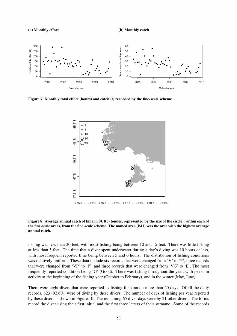
(a) Monthly effort

●

●

●

●●

●

●

●

●

●

●

●●

●

●

●

●

●

●

●

●●

●●

●●

●●

●

●●

●

●

●

●

●

●●

●

●

● ●●

●

●

2006 2007 2008 2009 2010

0

50

100

150

200

250

300

Calendar year

Tota

l mon

thly

effo

rt (

h)(b) Monthly catch

●

●

●

●●

●

●

●

●

●

●

●

●●

●

●

●●●

●

●

●●

●

●

●

●

●

●

● ●

●

●●

●●

●

●

●

●● ●

●

●

●

2006 2007 2008 2009 2010

0

10

20

30

40

50

60

Calendar year

Tota

l mon

thly

cat

ch (

tonn

es)

Figure 7: Monthly total effort (hours) and catch (t) recorded by the fine-scale scheme.

165.5°E 166°E 166.5°E 167°E 167.5°E 168°E 168.5°E 169°E

47.5

°S47

°S46

.5°S

46°S

45.5

°S

●

● ●●● ●

●

●●●

●●

●●

●●

●

●●●●

●

●●● ●

●

●

● ● ●● ●

●

●

●

●

●

●

●

25102050

F41

Figure 8: Average annual catch of kina in SUR5 (tonnes, represented by the size of the circle), within each ofthe fine-scale areas, from the fine-scale scheme. The named area (F41) was the area with the highest averageannual catch.

fishing was less than 30 feet, with most fishing being between 10 and 15 feet. There was little fishingat less than 5 feet. The time that a diver spent underwater during a day’s diving was 10 hours or less,with most frequent reported time being between 5 and 6 hours. The distribution of fishing conditionswas relatively uniform. These data include six records that were changed from ‘V’ to ‘P’, three recordsthat were changed from ‘VP’ to ‘P’, and three records that were changed from ‘VG’ to ‘E’. The mostfrequently reported condition being ‘G’ (Good). There was fishing throughout the year, with peaks inactivity at the beginning of the fishing year (October to February), and in the winter (May, June).

There were eight divers that were reported as fishing for kina on more than 20 days. Of all the dailyrecords, 823 (92.6%) were of diving by these divers. The number of days of fishing per year reportedby these divers is shown in Figure 10. The remaining 65 diver days were by 21 other divers. The formsrecord the diver using their first initial and the first three letters of their surname. Some of the records

53

(a) Depth

Feet

Fre

quen

cy

0 5 10 15 20 25 30

0

100

200

300

400

(b) Time underwater

Time underwater (h)

Fre

quen

cy

0 2 4 6 8 10

0

50

100

150

200

(c) Condition

P A G E

Num

ber

0

50

100

150

200

250

300

(d) Month

J F M A M J J A S O N D

Month

Num

ber

0

20

40

60

80

Figure 9: Distributions of non-catch related information from the fine-scale forms, showing (a) the depthof the fishing (feet), (b) the time spent underwater (hours), (c) the diving condition (Poor, Average, Good,Excellent), and (d) the month of the year. Data shown here are restricted to fishing in the 2005–06 to 2008–09fishing years, and exclude events from the beginning of the 2009–10 year.

Fishing year

Div

er

27 15 5 13

23

13 5 9 4

55

36 47

27 59 25 1

24 60 27

62 37 32 32

67 68 37 33

2006 2007 2008 2009

Other12345678

Figure 10: Number of daily records by diver and fishing year, for the eight divers that fished for kina onmore than 20 days, and for all other divers combined.

attributed to other divers may simply have been due to spelling errors. The number of days dived by otherdivers is also shown in Figure 10 for comparison. The fishing effort was unevenly distributed amongstthe divers, with Diver 7 and Diver 8 accounting for 43% of all the diving records between them. Thesesame two divers accounted for 47% of the catch recorded by the fine-scale programme.

54

3.8 CPUE

The relationship between the total monthly effort (see Figure 7(a)) and the total monthly catch (seeFigure 7(b)) is shown in Figure 11. Across all the fine-scale data, the average CPUE was 198 kg perhour. Although the reported fishing effort declined in 2007–08 and 2008–09, a consistent relationshipbetween the total effort in a month and the total catch appears to have been maintained. Time series ofthe CPUE are shown in Figure 12. There are coherent variations in the CPUE that last several months, forexample, there was a peak in CPUE in the second half of 2007 (Figure 12(a)), but there is no indicationof a consistent trend in CPUE across all areas. Similarly, although there are some months with lowCPUE for fishing in the F41 area, and two months with high CPUE at the start of the series, there is noimmediate evidence of a trend (Figure 12(a)).

●

●

●

●●

●

●

●

●

●

●

●

●●

●

●

● ●●

●

●

●●

●

●

●

●

●

●

●●

●

●●

●●

●

●

●

●●●

0 50 100 150 200 250 300

0

10

20

30

40

50

60

Monthly effort (h)

Mon

thly

cat

ch (

tonn

es)

●

●

2005−06, 2006−072007−08, 2008−09

Figure 11: Relationship between total monthly effort and total monthly catch, for all data from the 2005–06to 2008–09 fishing years. Data from the recent fishing years are shown with open symbols.

(a) All areas

●●●

●●●●

●●●

●

●

●

●

●

●

●

●

●

●●●

●●●

●

●●

●

●●

●

●

●●

●●

●●

●

●●●

●●

2006 2007 2008 2009 2010

0

100

200

300

400

500

Calendar year

Raw

CP

UE

(kg

per

hou

r)

●●●

●●●●

●●●

●

●

●

●

●

●

●

●

●

●●●

●●●

●

●●

●

●●

●

●

●●

●●

●●

●

●●●

●●

(b) F41 only

●●

●●●

●●●● ●

●

●

●●

●●

● ● ●

●

●

●●

●

●

●●

●

●

2006 2007 2008 2009 2010

0

100

200

300

400

500

Calendar year

Raw

CP

UE

(kg

per

hou

r)

●●

●●●

●●●● ●

●

●

●●

●●

● ● ●

●

●

●●

●

●

●●

●

●

Figure 12: Monthly time series of CPUE from all areas (a) and from F41 (b). The points mark the meanCPUE within each month, with the bars indicating the 90% quantile range.

The CPUE was consistent across most of the areas fished (Figure 13). For areas with an average CPUEof more than 120 kg per hour, there was no consistent relationship between catch and CPUE. For all sixareas where the total catch was less than 2 t, the average catch per unit effort was less than 120 kg perhour, and there were no other areas where the average CPUE was less than 120 kg per hour. These areaswith low CPUE and catch are likely to be areas where the fishers carried out some exploratory fishing,

55

●

●

●●

●●

●●

●●

●

●●

●● ● ●

● ●

● ●●

● ● ●

●

●

●●

●

●●●

●

0 50 100 150 200 250

010

030

050

0

Total catch (t)

Raw

CP

UE

(kg

per

hou

r)●

●

●●

●●

●●

●●

●

●●

●● ● ●

● ●

● ●●

● ● ●

●

●

●●

●

●●●

●●●

Figure 13: Catch per unit effort (CPUE) within each fine-scale area. For each area, the points mark theaverage CPUE, calculated from each daily diver record. The bars indicate the 90% confidence intervals.The open circles are two areas where there was only a single daily diver record.

but did not return because of the low success. In area F41, the total catch recorded during the periodcovered by the fine-scale data was 273 t, and the average catch per unit effort was 200 kg per hour. Thehigh catch in this area was not due to a high CPUE, but rather to high effort.

The relationships between the CPUE and other factors are shown in Figure 14. In most groups, therange of CPUE was large. The individual diver numbers in Figure 14(a) are the same as in Figure 10,and are sorted in order of increasing total number of diver days. The diver that dived the most had thehighest median CPUE, whereas the other divers, and the individual diver that dived the least, had thelowest CPUE. There was an increase in median CPUE with improved diving condition (Figure 14(b)),although the average CPUE (198 kg per hour) was within the inter-quartile range in all cases. There waslittle difference in CPUE between the Fiordland and Stewart Island regions (Figure 14(c)). The monthwith the lowest median CPUE was March (Figure 14(d)); this was also the month with the lowest fishingnumber of diver days (Figure 9(d)). The median CPUE ranged between 157 kg per hour in Marchand 250 kg per hour in August. There was no clear relation in the raw data between CPUE and timeunderwater (Figure 9(e)). Low CPUE was recorded on the six records that had a fishing depth of 5 feetor less, with high CPUE on the four records that had a fishing depth of over 25 feet (Figure 9(f)). Inthe depth range where most diving occurred, however, there was not a clear relationship between fishingdepth and CPUE.

3.8.1 CPUE modelling

Two similar models were fitted to two sets of CPUE data, both to explore the relationship betweenCPUE and available covariates and to determine whether there have been significant changes in CPUEover time. One model was fitted to all the dive-logger data, and one was fitted only to data from areaF41. The results of the model selection are given in Table 6. In both cases, diver number was thecovariate that explained the most deviance in the models (18.9% for all areas and 25.9% for area F41).This was followed by the condition, fishing year, and annual cosine covariates. The annual sine covariatewas included in the model of all areas, with the duration or time underwater covariate being includedin both models. The region covariate was presented for selection to the model of all areas, but was notretained, and fishing depth was also not selected for either model. Although the deviance explained bymany of the terms in the model of all areas was small, all the selected covariates were included in theBayesian model. For consistency, the same covariates were also included in the model of CPUE in the

56

(a) Diver

Diver

CP

UE

(kg

/hou

r)

0

100

200

300

400

500

600

Oth. 1 2 3 4 5 6 7 8

(b) Condition

Condition

CP

UE

(kg

/hou

r)

0

100

200

300

400

500

600

P A G E

(c) Region

Region

CP

UE

(kg

/hou

r)

0

100

200

300

400

500

600

F S

(d) Month

Month

CP

UE

(kg

/hou

r)

0

100

200

300

400

500

600

J F M A M J J A S O N D

(e) Time

Time underwater (h)

CP

UE

(kg

/hou

r)

0

100

200

300

400

500

600

0 2 4 6 8 10

(f) Depth

Depth (m)

CP

UE

(kg

/hou

r)

0

100

200

300

400

500

600

0 10 20 30

Figure 14: Boxplots giving the relationship between CPUE and other factors. The line across the boxplotsmarks the median value of the CPUE with each group, the box indicates the inter-quartile range, and theline extends to the full range.

F41 area, even though the annual sine term was not included by the automatic selection process in thatcase. Including both the cosine and sine terms allows for selection of both the amplitude and the phaseof any annual cycles in CPUE. The duration of the diving was offered to both models as a check fornonlinearity in the relation between duration of diving and catch, but it explained little of the deviance.Duration was not included in the final models.

Having selected the covariates, the Bayesian models were run. For all the model parameters the finalchains passed the Heidelberger and Welch stationarity test (Heidelberger & Welch 1983), and there wasno evidence of problems with model convergence. Example samples of model parameters are given inFigure 15. The posterior densities derived from both chains overlap closely, and the traces of the chainsshow no evidence of non-convergence. The plots show the posterior density of the multiplicative 2009year effect. In the model of all the areas, the best estimate was that in 2008–09 the CPUE was 95% ofwhat it had been in 2005–06. This decrease was not significant. When the model was restricted to themost heavily fished area (F41), the best estimate was that in 2008–09 the CPUE was 77% of what ithad been in 2005–06. In this area, the model found that there was a 95.3% probability that the CPUEhad decreased between 2005–06 and 2008–09. Most of the decrease occurred between the 2006–07 and2007–08 fishing years.

To further check the model fit, standardised residuals were compared with a normal distribution(Figure 16). In both models, the sample quantiles (qs) and the theoretical quantiles (qt) were notsignificantly different (qs − qt = 0) over most of the data (qt < 2). At higher values the distributionsdiverged, with qs > qt . There were more unusually high values of CPUE in the data than accounted for

57

Table 6: Summary of covariate selection, with ANOVA tables showing the decrease in deviance as furtherterms are added to the models. For each covariate, the table gives the number of degrees of freedom (DOF),the deviance explained by adding that covariate to the model, the residual deviance, and the percentagedeviance explained. The deviance and the residual deviance in these tables have been divided by 1000.Covariates are listed in the order in which they were added to the model by the step routine.

(a) All areasDOF Deviance Resid. dev. % explained

2622Diver 8 495 2127 18.87Condition 3 141 1986 5.37Fishing year 3 21 1965 0.82Annual cosine 1 8 1957 0.31Annual sine 1 68 1889 2.58Duration 1 13 1876 0.49

(b) F41 onlyDOF Deviance Resid. dev. % explained

557Diver 8 144 412 25.93Condition 3 20 392 3.68Fishing year 3 32 360 5.67Annual cosine 1 12 348 2.14Duration 1 10 339 1.75

(a) All areas

2.5%

Med

ian

97.5

%

1000

2000

3000

4000

Sam

ple

num

ber

0.4 0.6 0.8 1.0 1.2 1.4

exp(β2009)

0

1

2

3

4

5

6

Pro

babi

lity

dens

ity

(b) F41 only

2.5%

Med

ian

97.5

%

1000

2000

3000

4000

Sam

ple

num

ber

0.4 0.6 0.8 1.0 1.2 1.4

exp(β2009)

0.0

0.5

1.0

1.5

2.0

2.5

3.0

3.5

Pro

babi

lity

dens

ity

Figure 15: Posterior density of the multiplicative 2009 year effect, being the ratio of the modelled CPUE in2008–09 to the modelled CPUE in 2005–06. Results are shown from the model of all areas (a), and restrictedto data from F41 (b). The solid and dashed lines show the posterior density from the two independentMCMC chains, while the traces of the two chains are shown in the background in gray.

by the model. For the model restricted to F41, this divergence was associated with only two data points.

A full summary of the fitted parameters from the two models is given in Table 7. The parametersestimated from the two models were similar. In all cases, other than the Diver 4 effect, the mean valueof the parameter from the all areas model fell within the 95% confidence interval of the same parameterestimated from the F41 model. The uncertainty in the parameters from the F41 model was generallyhigher, reflecting the fact that the F41 model was fitted to a smaller dataset.

Which diver was fishing was the covariate that explained most of the model deviance during modelselection, and was the covariate associated with the strongest effects. Other than Diver 3, all divers hada lower CPUE than Diver 8. When one of the ‘Other’ divers was fishing the CPUE would be 52% of theCPUE when Diver 8 was fishing (all else being equal).

58

(a) All areas

● ● ● ●●●●●●●●●●●●●●●●●●●●●●●●●●●●●●●●●●●●●●●●●●●●●●●●●●●●●●●●●●●●●●●●●●●●●●●●●●●●●●●●●●●●●●●●●●●●●●●●●●●●●●●●●●●●●●●●●●●●●●●●●●●●●●●●●●●●●●●●●●●●●●●●●●●●●●●●●●●●●●●●●●●●●●●●●●●●●●●●●●●●●●●●●●●●●●●●●●●●●●●●●●●●●●●●●●●●●●●●●●●●●●●●●●●●●●●●●●●●●●●●●●●●●●●●●●●●●●●●●●●●●●●●●●●●●●●●●●●●●●●●●●●●●●●●●●●●●●●●●●●●●●●●●●●●●●●●●●●●●●●●●●●●●●●●●●●●●●●●●●●●●●●●●●●●●●●●●●●●●●●●●●●●●●●●●●●●●●●●●●●●●●●●●●●●●●●●●●●●●●●●●●●●●●●●●●●●●●●●●●●●●●●●●●●●●●●●●●●●●●●●●●●●●●●●●●●●●●●●●●●●●●●●●●●●●●●●●●●●●●●●●●●●●●●●●●●●●●●●●●●●●●●●●●●●●●●●●●●●●●●●●●●●●●●●●●●●●●●●●●●●●●●●●●●●●●●●●●●●●●●●●●●●●●●●●●●●●●●●●●●●●●●●●●●●●●●●●●●●●●●●●●●●●●●●●●●●●●●●●●●●●●●●●●●●●●●●●●●●●●●●●●●●●●●●●●●●●●●●●●●●●●●●●●●●●●●●●●●●●●●●●●●●●●●●●●●●●●●●●●●●●●●●●●●●●●●●●●●●●●●●●●●●●●●●●●●●●●●●●●●●●●●●●●●●●●●●●●●●●●●●●●●●●●●●●●●●●●●●●●●●●●●●●●●●●●●●●●●●●●●●●●●●●●●●●●

●●●●●●●●●●●●●

●●●●●

●●●●●●

●●

●

●

●

●

01

23

45

−3 −2 −1 0 1 2 3

Theoretical quantiles qt

q s−

q t

(b) F41 only

●● ● ● ● ●●●●●●●●●●●●●●●●●●●●●●●●●●●●●●●●●●●●●●●●●●●●●●●●●●●●●●●●●●●●●●●●●●●●●●●●●●●●●●●●●●●●●●●●●●●●●●●●●●●●●●●●●●●●●●●●●●●●●●●●●●●●●●●●●●●●●●●●●●●●●●●●●●●●●●●●●●●●●●●●●●●●●●●●●●●●●●●●●● ● ●

●

●

●

01

23

4

−3 −2 −1 0 1 2 3

Theoretical quantiles qt

q s−

q t

Figure 16: Model diagnostics, showing the distribution of residuals compared with the theoreticaldistribution. The difference between the quantiles of the standardised residuals (qs) and the theoreticalquantiles (qt ) from a normal distribution, are plotted against the theoretical quantiles. The difference iscalculated for 2000 samples from the MCMC chains, with the dots marking the median values, and thelines indicating the 95% confidence intervals. If the data followed the theoretical distribution, the line atqs −qt = 0 would fall within the confidence intervals.

As may be expected, the CPUE was less when the diving conditions were poor, and was greater when thediving conditions were excellent (although the difference was only significant for the all years model).There was not a significant difference in the CPUE between diving during average or good conditions. Inneither of the models were there any significant year effects. The mean value of the multiplicative 2009year effect (relative to 2006) was less than one for both models, with a mean value of 0.95 for the modelof all areas, and 0.77 for the model restricted to area F41. There was seasonal variation in the CPUE,with a peak in CPUE between October and December (Figure 17).

(a) All areas

Month of year

Mul

tiplic

ativ

e ef

fect

0.8

0.9

1.0

1.1

1.2

1.3

J F M A M J J A S O N D

(b) F41 only

Month of year

Mul

tiplic

ativ

e ef

fect

0.8

0.9

1.0

1.1

1.2

1.3

J F M A M J J A S O N D

Figure 17: Relative variation in the CPUE through the year.

59

Table 7: Summary of estimated model parameters from the model of all areas and of F41. The coefficientsof the model covariates have been exponentiated so that they may be interpreted as multiplicative effects(for example in the all areas model, if Diver 1 is fishing the CPUE is 51% of the CPUE if Diver 8 is fishing,all else being equal). The base case of the model is a day of fishing by Diver 8, with 6 hours time underwater,in good diving conditions, in 2006, at the beginning of the year.

Parameter All areas F41

Mean 2.5% 97.5% Mean 2.5% 97.5%

Intercept 251.11 222.20 284.18 345.39 271.56 439.37

Diver coefficient (relative to Diver 8)Diver 1 0.51 0.44 0.60 0.58 0.43 0.79Diver 2 0.76 0.66 0.87 0.66 0.50 0.86Diver 3 0.93 0.84 1.03 0.92 0.75 1.11Diver 4 0.77 0.70 0.83 0.63 0.54 0.74Diver 5 0.73 0.67 0.78 0.63 0.54 0.73Diver 6 0.85 0.79 0.92 0.77 0.66 0.89Diver 7 0.67 0.62 0.71 0.64 0.56 0.73Other 0.52 0.47 0.58 0.52 0.44 0.63

Condition coefficient (relative to Good)Poor 0.85 0.76 0.96 0.86 0.65 1.14Average 0.93 0.83 1.05 0.81 0.64 1.02Excellent 1.13 1.00 1.28 1.07 0.82 1.39

Year coefficient (relative to 2006)2007 1.02 0.91 1.14 0.98 0.80 1.212008 0.97 0.85 1.11 0.74 0.53 1.022009 0.95 0.82 1.10 0.77 0.57 1.05

Annual harmonicCosine coefficient 1.06 0.98 1.13 1.14 0.99 1.31Sine coefficient 0.92 0.86 0.98 0.98 0.86 1.12

Standard deviation of errorsResidual, σ 0.31 0.30 0.33 0.29 0.26 0.33Form, σ f 0.26 0.22 0.30 0.24 0.17 0.33Area, σa 0.12 0.02 0.28

3.9 Customary data

The data on customary kina harvest consist of quarterly returns of approved and actual harvest. In thedata provided, there were 737 returns from the third quarter of 1998 to the final quarter of 2009. Thedata were truncated to data from the 1999–2000 to 2008–09 fishing years, dropping one record from thethird quarter of 1998 and 18 records from the final quarter of 2009. For each record the data includedboth the approved and the actual harvest. For 147 records the actual harvest was blank, and these recordswere excluded. For a further 34 records the actual harvest was zero. All the people spoken to (PouHononga, customary fishers, Kaitiaki) emphasised that the reported data do not represent the full extentof the customary harvest.

Data were reported using a range of units (Table 8), with reporting of harvest as number of kina or inkilogrammes being most frequent. There were some reports of harvest using a range of container types,but these accounted for only a small proportion of the reported actual harvest. After the data had beengroomed, there remained 55 records that did not have a unit type. These records have not been includedin tables of total catch.

Customary harvest of kina was reported under three regulations, with most reporting being under the

60

Table 8: Units used for reporting actual customary catch. This summary was prepared after the unit datahad been groomed.

Units Records Total

Number Tonnes

Missing 57 18 185 0

BAG 50 183 4.58BIN 7 17 0.42KG 137 35 880 35.88NO. 299 508 549 126.27SAC 27 157 3.92SUG 4 3 0.08Missing 1 0 0

Kaimoana and Section 27A regulations (Table 9). There were relatively few reports made under theSouth Island regulations. On average, actual harvests reported under the Kaimoana regulations wereof over 500 kg of kina, whereas actual harvests reported under the section 27A regulations were, onaverage, 100 kg. Most of the reported actual harvest was made under the Kaimoana regulations. Thereporting of customary kina harvest has increased markedly in recent years (Figure 18), with the totalactual harvest reaching 50 t in 2007–08 and 2008–09. In 2008–09, over 95% of the actual harvest wasunder the Kaimoana regulations. All participants spoken to during the interviews emphasised that not allcustomary harvest is reported. The extent of the under-reporting is unknown, and all figures given herecan only be regarded as a minimum harvest.

Table 9: Regulations used for reporting customary catch.

Regulation Records Average weight (kg) Total weight (t)

Kaimoana 271 561 135South Island 53 227 8Regulation 27A 258 115 29

1999

2000

2001

2002

2003

2004

2005

2006

2007

2008

2009

Regulation 27ASouth IslandKaimoana

Fishing year

Tonn

es

0

10

20

30

40

50

60

Figure 18: Reported actual customary harvest of kina (tonnes) by year and regulation.

The actual harvest has been predominantly reported from areas SUR2A and SUR2B (Table 10). Acrossall the data, 65% of the reported actual harvest has been from those two areas. The 2008–09 reportedactual customary harvest in SUR2A of 19.9 t compares with the landed commercial catch of 20.1 t in thesame year. In SUR2B there has only been a few commercial vessels operating, with the highest landedcatch in recent years being 11.7 t in 2006–07, less than the 2008–09 reported actual customary harvest of13.7 t. In SUR7A, a single customary fisher spoken to during the interviews estimated that they harvest

61

20 t of kina a year. This compares with a total reported actual customary harvest from SUR7A of 3.9 t,over all years.

The customary data include records that have an approved harvest, but no recorded actual harvest. Duringthe 2008–09 fishing year, the total recorded actual harvest was 49.6 t, while the total approved harvestwas 62.6 t, 26% higher. Similarly, in 2008–09 the recorded harvest was 49.7 t while the approved harvestwas 65.9 t. For 49.7 of records the actual and approved harvests were the same.

Table 10: Reported actual customary harvest by QMA. The harvest is given in t, and is rounded to thenearest 100 kg. A zero harvest is indicated where a harvest of less than 50 kg was reported.

Fishing year QMA Total1A 1B 2A 2B 3 5 7A 7B 8 9

1998–99 0.0 0.0 0.01999–00 0.8 0.0 0.0 0.82000–01 0.0 2.2 0.0 0.1 2.32001–02 0.0 0.2 1.0 1.22002–03 1.6 0.5 0.0 0.6 0.3 3.02003–04 2.4 0.1 2.2 1.3 6.02004–05 3.7 0.2 4.5 1.0 0.0 9.42005–06 2.1 5.9 4.2 0.1 0.2 0.0 12.52006–07 2.7 6.0 16.3 8.6 0.4 0.1 2.4 0.1 36.42007–08 4.6 10.9 19.2 11.6 1.0 1.9 0.6 0.0 49.92008–09 4.5 9.2 19.9 13.7 0.2 1.8 0.0 0.0 0.3 49.6

3.10 Recreational fishery

Currently, the only comprehensive reporting of catch occurs in the commercial fishery. Interviews withcustomary fishers and Kaitiaki indicated that much of the customary kina harvest is likely taken under theAmateur Fishing Regulations. There is some information provided for recreational harvest levels of kinaaround New Zealand from recreational fishing surveys. Bradford (1998) derived estimates of recreationalharvest levels for a range of fish and shellfish, including kina, from a national marine recreationalfishing diary survey, with mean weights estimated from a boat ramp survey conducted in the sameyear. However, estimates of total harvest based on this survey were not considered reliable (Ministryof Fisheries 2009). Boyd & Reilly (2002) estimated the national recreational harvest for a wide rangeof fish and shellfish species using the combined results from three separate but related surveys: a face toface nationwide survey, a boat ramp survey to estimate the mean weight of recreationally harvested fishand shellfish, and a detailed diary data of recreational harvest from a nationwide sample of recreationalfishers, with demographic data used to interpret the harvest of diarists.

The recreational harvest estimated by Boyd & Reilly (2002) for kina in 2000 is shown in Table 11. Theresults of the boat ramp survey were used to convert the harvest in numbers to total harvest weight.Estimated recreational harvest was high in FMAs 1 and 2 relative to other FMAs. The estimatedrecreational harvest of 445.2 t in SUR1 in 2000 was almost three times the current combined recreationalallowance for SUR1A and 1B of 155 t, at least double the current combined TACC of 180 t, and equatedto about 90% of the current combined TAC for SUR1A and 1B (see Table 2, Table 11). The catch inSUR2 in 2000 was well over double the current combined recreational allowance for SUR2A and SUR2Bof 95 t, and the current combined TACC of 110 t, equating to about 83% of the current combined TACfor SUR2A and 2B (see Table 2, Table 11). These estimates suggest that recreational harvest levels maycomprise a large proportion of the total harvest of kina in some QMAs.

62

Table 11: Estimated recreational harvest of kina in 2000 (Boyd & Reilly 2002).

Area Number of kina (x 1000) c.v. (%) Catch (t)

SUR1 1793 35 445.2SUR2 1026 57 254.7SUR3 8 58 2.0SUR5 70 101 0.5SUR7 2 101 17.4SUR8 85 85 21.1SUR9 82 67 20.4

4. DISCUSSION

4.1 Kina biology and ecology

There is a large amount of information on the biology and ecology of kina. A persistent theme was thespatial variability in a range of kina life-history parameters. Research specific to kina fisheries in NewZealand has investigated improving roe colour and taste, and enhancing roe recovery. However, asidefrom work including that by McShane & Naylor (1991) and McShane et al. (1993), there is little fisheriesspecific information on abundance and distribution. Recent surveys of subtidal algae and invertebrateshave provided information on the associations between kina and other environmental and biologicalfactors (Shears 2007, 2010). These may prove useful in modelling the spatial distributions of kina aroundthe New Zealand coastline.

Interviews with fishers highlighted perceived negative associations between paua and kina. There isevidence to support these observations from New Zealand and overseas, suggesting that urchins canlimit abalone populations (Andrew et al. 1998, Naylor & Gerring 2001, Konstantin et al. 2001). Kinaalso interact with lobster and fish populations, as large lobster and reef fish will eat small kina. Fishinghas reduced the predation pressure on kina, which is believed to have led to the formation of kina barrensin northern New Zealand (e.g., Babcock et al. 1999, Shears & Babcock 2002, 2003). Fishing of kina willhave wider ecosystem effects on other species. These potential effects are currently not considered aspart of the management of either kina or of other subtidal-reef fisheries.

4.2 Commercial fishery

The kina fishery in New Zealand currently harvests some 750 t of kina per year, compared with a TotalAllowable Commercial Catch (TACC) of 1147 t. The commercial industry is small, with 75% of the catchin the 2008–09 fishing year being harvested by nine vessels. Commercial kina catch is concentrated infour QMAs, with annual catches greater than 50 t restricted to single statistical areas within each ofthese four QMAs. Information from fisher interviews assisted with the interpretation of catch effort data,identifying seasonal variation in roe recovery and market demand as drivers of monthly catch patternsin many QMAs. The industry appears to have restructured in response to the introduction of kina intothe QMS, with a reduction in the number of vessels participating, and an increase in the average catchper vessel. In many QMAs there has been a corresponding increase in the raw catch per unit effort, andthis may be driven by changes in the efficiency of the fishery, rather than an increase in the abundance ofkina. Andrew (2000) advised caution in using catch rate information gathered at broad spatial scales forstock assessment of sedentary invertebrate species such as kina.

63

Although breath-hold diving is the main harvest method for kina, there has been some dredging forkina in SUR1B and SUR7A. Dredging contributed to the bulk of catch from SUR7A in the 1996–97fishing year (63%), and continued to dominate the catch until the 1998–99 fishing year when it beganto decline. In recent years, there has been a voluntary ban on kina dredging. Information from fisherinterviews suggested that a lack of suitable habitat limited kina presence and abundance in SUR3, andkina occurring at depths less accessible to breath-hold divers in SUR2A and SUR2B made kina in theseareas uneconomic to fish.

Interviews with fishers and processors provided information on key drivers for kina fishing, particularlyroe recovery. Fishers explained how the small-scale and relatively low economic value of the fisherylimits the type of information that can be collected to monitor the sustainability of the fishery. Mostfishers interviewed suggested fine-scale reporting could provide information at a more useful scale thanthat occurring under the current reporting.

The fine-scale data that have already been collected allowed a more detailed analysis of patterns in CPUEfrom a single fishing company in the SUR5 fishery. Over the four years for which data were available,there was some evidence of a decline in CPUE. The best estimate was that in 2008–09 the CPUE in themost heavily fished area (F41) was 77% of what it had been in 2005–06. From the model, there was a95.3% probability that the CPUE had decreased between 2006 and 2009. In the model of all areas, therewas little evidence of a decrease in CPUE over the time period covered by the data. This illustrates thepotential importance of fine scale data collection.

The fine-scale data illustrate the concentration of the fishery: two divers accounted for 46% of the catchreported by the fine-scale programme. The factor that explained most of the variability in CPUE wasthe diver. The analysis assumed that diver skill was constant throughout the period. It is possible thatchanges in the fitness of a single diver could lead to apparent changes in the CPUE of the kina fisherywithin a QMA. Similarly, although there was some fishing in a range of fine-scale areas, the fishing wasconcentrated, with close to one-quarter of all the catch reported by the fine-scale programme being froma single fine-scale area (paua statistical area F41, Green Islets). The concentration of effort in the F41area was not related to it having an unusually high CPUE. According to the fisher concerned, it wasrather driven by access: the F41 area is sheltered from weather from the north, and is closer to port thanother areas along the southern Fiordland coast.

The importance of individual divers for explaining variation in CPUE highlights the unreliability ofaggregated data from the Catch Effort Landing Return forms for monitoring for changes in CPUE.

4.3 Customary fishery

According to discussions with customary fishers and Kaitiaki, customary catch is currently under-estimated in the catch reported to the Ministry of Fisheries, as much of the catch is caught underthe Amateur Fishing Regulations that have no reporting requirement. Further, in areas that are notcovered by the Kaimoana or South Island Customary Fishing regulations, customary fishing takes placeunder Regulation 27A of the Amateur Fishing Regulations, where, unless specified by the representativeauthorised to issue permits for customary fishing, there is no mandatory requirement to report catch.While the data that are available demonstrate that in some areas the scale of the customary fishery issimilar to the scale of the commercial fishery (e.g., in SUR2A reported customary harvest in 2008–09was 19.9 t and landed commercial catch was 20.1 t), an estimate of customary catch provided by oneinterviewee was that their catch was greatly in excess of the reported catch. The customary data mayonly be considered as minimum catches that likely underestimate actual customary harvest levels forsome areas.

64

Erosion of customary values in favour of commercial interests was a key issue for customary fishers.Access to kina stocks was also highlighted as an area of concern, especially as fishers consideredkina abundance had decreased in some areas. Some customary fishers spoken to suggested that catchinformation is also required from the recreational sector, and, if data in the commercial fishery for kinaare collected at a finer spatial scale, this needs to correspond with current fine-scale data collection forspecies such as paua to define the spatial extent of these fisheries relative to each other.

Importantly, although there are few data to quantify levels of customary fishing for kina around NewZealand, interviews with Kaitiaki and customary fishers indicate the high level of significance of kina toMaori, to maintain the mana of the marae and the people.

4.4 Management of kina fisheries

A review of management and monitoring in other fisheries for sedentary invertebrates, including urchins,notes that small-scale, spatially structured fisheries for sedentary species such as kina are prone to serialdepletion, with examples of urchin fisheries having declined or collapsed elsewhere in the world (e.g.,Sloan et al. 1985). Many fisheries for sedentary invertebrates, recognising that conventional fisheriesmanagement is inappropriate, now manage their fisheries, and collect information for management, atfiner spatial scales (Orensanz et al. 2005, Harrington et al. 2008).

Andrew (2000) stated a decade ago that management of the kina fishery in New Zealand was inadequate,and suggested the use of management plans that would set local catch limits, and prescribe patterns offishing to enhance roe quality and reduce the risk of serial depletion. He suggested that the followingare the key attributes required for improved management of the kina fishery: 1) the ability to managekina at the appropriate spatial scale; 2) continuity of management through time; 3) a property rightsinstitution that rewards commitment to the fishery; and 4) through the allocation of property rights, theestablishment of clear rights and responsibilities of stakeholders.

Andrew’s (2000) first recommendation to manage kina at the appropriate spatial scale, is still to be met.However, since QMS introduction, the Kina Industry Council, representing the interests of kina quotaowners, has evolved, and in accordance with Andrew (2000), provide a means for cooperation in thefishery, while the introduction of kina into the QMS allows for continuity of management through time,places kina within a property rights institution (thereby providing incentives to invest in the fishery), andestablishes stakeholder rights and responsibilities. Therefore, Andrew’s (2000) second, third, and fourthrecommendations above are satisified.

Since QMS introduction, kina have been managed at the scale of QMA, which is not appropriate due tothe sedentary nature, aggregated distribution, and local scale variation in demography of kina (Andrew2000). As a consequence of these characteristics, kina will have varying responses to fishing, resulting insome populations being productive and others not (Andrew 2000). Therefore, Andrew (2000) advocatedthe gathering of information on kina abundance and response to fishing at small spatial scales.

Fisheries plans can provide a framework within which fine-scale management of the fishery can bedeveloped with the input of all stakeholders. At present, the direction of fisheries management in NewZealand is via national fisheries plans. Within fisheries plans, the value different stakeholders derive fromthe fishery can be identified, objectives to get the best value from the fishery can be set, and managementcan be designed to achieve these objectives (Ministry of Fisheries 2010a). It is anticipated kina willcome under a national fisheries plan to be developed on shellfish (A. Frazer, Ministry of Fisheries, pers.comm., 25 August 2010).

65

4.5 Monitoring

The sedentary nature of kina, their vulnerability to serial depletion, the potentially high levels ofnon-commercial catch in some QMAs, and the potential for resource conflict between fishery sectorssuggests that better information on the spatial extent of fishing for kina is needed across all fisherysectors (commercial, customary, and recreational). To date, the only monitoring of the commercial kinafishery has been monitoring landings against the Total Allowable Commercial Catch (TACC) for kina.Therefore, the Ministry of Fisheries has no information on the sustainability of current catch levels orTACCs (Ministry of Fisheries 2009). Andrew (2000) noted catch and effort data collected at the scaleof the QMA is not useful for managing the kina fishery, and suggested developing an accurate fine-scalecatch and effort reporting scheme for fisheries assessment. A first step suggested for monitoring wouldbe via fisher dependent data collection, due to the prohibitive cost of scientific biomass surveys relativeto the commercial value of the kina fishery (Andrew 2000).

Some fine-scale recording of kina fishing has been occurring voluntarily in the SUR5 fishery for the lastfour years. Until now, this fine scale information has not been reported, except as an aggregated monthlycatch to the Ministry of Fisheries. If the collection of the fine-scale data are to be useful to the fishers,and to the management of the fishery, it is important that more frequent analysis is undertaken. In theCoromandel scallop fishery, fine-scale monitoring is now carried out routinely, with weekly reportingof data back to fishers. This allows the fishers to respond immediately to in-season changes in CPUE,setting areas aside if the CPUE falls below agreed levels.

An important feature of the voluntary fine-scale reporting, using the Paua Catch Effort Landing Return(PCELR) forms, is that data are collected on the catch and effort of individual divers. As the personwho is diving has a large effect on the CPUE, it is essential that data are collected at the diver level.The importance of diver identity to analysis of CPUE is also found in paua fisheries (e.g., McKenzie& Smith 2009). Data loggers have been developed for use in the paua fishery, to allow data collectionfrom the fishery at a relevant spatial scale. These use GPS and depth loggers to collect information oneach individual dive. They are expected to allow reef-scale resolution of paua catch and effort. Their usefor fisheries management is currently in development. If successful, it may be possible for them to beadopted by the kina fishing industry. An advantage of the loggers is that data are recorded with latitudeand longitude position. This would allow the spatial extent of the kina fishery to be properly understood,and would help prevent changes in kina abundance remaining undetected due to serial depletion.

A further source of monitoring information would be shed sampling of kina size, and recording of roerecovery rates. This would give information on non-biomass related changes in the fishery. Consideringthat roe recovery and roe quality are important to the economics of the kina fishery, shed sampling of roerecovery and size structure was suggested by Andrew (2000) to provide important information to assessmanagement impacts. Roe recovery is thought to respond to changes in kina abundance, with a decreasein kina densities leading to an increase in recovery rates. Any monitoring of either size or roe recoveryshould be done at a spatial scale appropriate to kina. Fishery independent surveys for areas where catchis concentrated could be carried out in future based on information gathered on catch and effort. Thescale of current catch and effort information is too large to allow survey effort to be efficiently targeted.

Although recreational harvest of kina is estimated to be almost equivalent to the total allowable catch inSUR1A, SUR1B, SUR2A and SUR2B, there are no data gathered on any recreational fishing activity inNew Zealand, aside from estimates by Boyd & Reilly (2002). Considering the shift in attitudes requiredto implement reporting in any recreational fishery in New Zealand, consideration in the short-term couldinstead be given to getting better estimates of recreational kina harvest in areas of the country wherecatches are estimated to be high, focusing on, if possible, estimates of catch at finer-spatial scales.

66

Data gathered to monitor customary kina harvest are currently carried out at the scale of QMA. However,future consideration could be given to collecting customary data corresponding to the scale commercialdata is gathered at, to provide better information on harvest location, and to assess fishing pressure ondiscrete stocks, considering the importance of kina to all fisheries sectors.

5. ACKNOWLEDGMENTS

We especially thank all the interview participants (Chatham Islands, Southland, Nelson/Marlborough,and the Coromandel) who willingly gave their time to provide valuable insight into the kina fishery inNew Zealand, and give constructive feedback.

We thank staff at the Ministry of Fisheries for assistance with contacting fishers for the interviewcomponent of this report, particularly George Ririnui, Carl Baker, and Otene Rewiti (Ministry ofFisheries), and Nigel Scott (Te Runanga o Ngai Tahu). Robert Akuhata (Ministry of Fisheries)provided Dragonfly with data on the customary fishery. Ministry of Fisheries staff provided usefulbackground information, particularly Allen Frazer, Mark Geytenbeek, and Alan Moore. Other Ministryof Fisheries staff also provided information for the project; Laura Mitchell, Martin Williams, Phillip Kerr,Dave O’Dea, Murray Pridham, Nathan Walker, Geoff Clark, and Peter Hyde. Dean Savage provideduseful historical background information on the SUR2 kina fishery. The project also benefited fromuseful discussions and assistance from Kate Bartram (SeaFIC), and Alan Riwaka (Te Ohu Kaimoana).Discussion with Clive Pomare assisted with subsequent fisher interviews on the Chatham Islands. PaulMcShane and Reyn Naylor (NIWA) gave permission for us to cite their work on kina in New Zealand.We would like to thank the South Island Kina Association for the provision of fine-scale reporting datafor analysis, espcecially Russell Bell and Jason McMath (WHK - Invercargill) who provided fine-scaledata to Dragonfly with the permission of the fisher concerned. We are also grateful to Peter “Herb”Herbert (Sea Urchin New Zealand Limited) and Phil James (The Norwegian Institute of Food, Fisheriesand Aquaculture Research) for making their research available for use in this report.

Finlay Thompson of Dragonfly assisted with data preparation and analysis. We are grateful to membersof the Shellfish Working Group for their insight, and to Richard Ford of the Ministry of Fisheries for hisdetailed comments on the draft manuscript.

This research was funded by Ministry of Fisheries project SUR2009/01.

6. REFERENCES

Abraham, E. (2007). Sea-urchin feeding fronts. Ecological Complexity 4(4): 161–168.Akaike, H. (1974). A new look at the statistical model identification. IEEE Transactions on Automatic

Control 19(6): 716–723.Anderson, M.; Millar, R. (2004). Spatial variation and effects of habitat on temperate reef fish

assemblages in northeastern New Zealand. Journal of Experimental Marine Biology and Ecology305(2): 191–221.

Andrew, N. (1986). The interaction between diet and density in influencing reproductive output inthe echinoid Evechinus chloroticus (Val.). Journal of Experimental Marine Biology and Ecology97(1): 63–79.

Andrew, N. (1988). Ecological aspects of the common sea urchin, Evechinus chloroticus, in northernNew Zealand: A review. New Zealand Journal of Marine and Freshwater Research 22(3): 415–426.

Andrew, N. (2000). Sea urchin fisheries: their status and management with special reference to the

67

New Zealand kina fishery. Unpublished report prepared for the Ministry of Fisheries and Te OhuKaimoana.

Andrew, N.; Agatsuma, Y.; Ballesteros, E.; Bazhin, A.; Creaser, E.; Barnes, D.; et al. (2002). Status andmanagement of world sea urchin fisheries. Oceanography and Marine Biology: An Annual Review40: 343–425.

Andrew, N.; Choat, J. (1982). The influence of predation and conspecific adults on the abundance ofjuvenile Evechinus chloroticus (Echinoidea: Echinometridae). Oecologia 54(1): 80–87.

Andrew, N.; Choat, J. (1985). Habitat related differences in the survivorship and growth of juvenile seaurchins. Marine Ecology Progress Series 27: 155–161.

Andrew, N.; MacDiarmid, A. (1991). Interrelations between sea urchins and spiny lobsters innortheastern New Zealand. Marine Ecology Progress Series 70(3): 211–222.

Andrew, N.; MacDiarmid, A. (1999). Sea urchin fisheries and potential ecological interactions with akina fishery in Fiordland. Conservation Advisory Science Notes 266. 12 p.

Andrew, N.; Worthington, D.; Brett, P.; Bentley, N.; Chick, R.; Blount, C. (1998). Interactions betweenthe abalone fishery and sea urchins in New South Wales. New South Wales Fisheries Final ReportSeries No. 12. 108 p.

Annala, J. (1995). Report from the Fishery Assessment Plenary, May 1995: stock assessments and yieldestimates. (Unpublished report held in NIWA library, Wellington.)

Ayling, A. (1978). The relation of food availability and food preferences to the field diet of an echinoidEvechinus chloroticus (Valenciennes). Journal of Experimental Marine Biology and Ecology33(3): 223–235.

Babcock, R.; Kelly, S.; Shears, N.; Walker, J.; Willis, T. (1999). Changes in community structure intemperate marine reserves. Marine Ecology Progress Series 189: 125–134.

Barker, M. (2001). The ecology of Evechinus chloroticus. In, Lawrence, J. (Ed.), Edible sea urchins:biology and ecology, pp. 245–260. Elsevier, Amsterdam.

Barker, M.; Keogh, J.; Lawrence, J.; Lawrence, A. (1998). Feeding rate, absorption efficiencies, growth,and enhancement of gonad production in the New Zealand sea urchin Evechinus chloroticusValenciennes (Echinoidea: Echinometridae) fed prepared and natural diets. Journal of ShellfishResearch 17: 1583–1590.

Beverton, R.; Holt, S. (1957). On the dynamics of exploited fish populations. Ministry of Agriculture,Fisheries, and Food, London.

Boyd, R.; Reilly, J. (2002). 1999/2000 National marine recreational fishing survey: harvest estimates.Unpublished report on project REC98/03 held by the Ministry of Fisheries, Wellington.

Bradford, E. (1998). Harvest estimates from the 1996 national marine recreational fishing surveys. NewZealand Fisheries Assessment Research Document 98/16. 27 p. (Unpublished report held in NIWAlibrary, Wellington.)

Breen, P.A. (2005). Managing the effects of fishing on the environment: what does it mean for the rocklobster (Jasus edwardsii) fishery? New Zealand Fisheries Assessment Report 2005/53. 45 p.

Brewin, P.; Lamare, M.; Keogh, J.; Mladenov, P. (2000). Reproductive variability over a four-year periodin the sea urchin Evechinus chloroticus (Echinoidea: Echinodermata) from differing habitats inNew Zealand. Marine Biology 137(3): 543–557.

Buchanan, J. (1966). The biology of Echinocardium cordatum (Echinodermata: Spatangoidea) fromdifferent habitats. Journal of the Marine Biological Association of the United Kingdom 46(1):97–114.

Buisson, P.; Barker, M. (2001). Enhancing gonad quality in Evechinus chloroticus (Val.) collected fromDoubtful Sound, New Zealand. In, Barker, M. (Ed.), Echinoderms 2000: proceedings of the 10thinternational conference, p. 423. Swets & Zeitlinger, Lisse.

Byrne, M. (1990). Annual reproductive cycles of the commercial sea urchin Paracentrotus lividus froman exposed intertidal and a sheltered subtidal habitat on the west coast of Ireland. Marine Biology104(2): 275–289.

Caddy, J. (1975). Spatial model for an exploited shellfish population, and its application to the Georges

68

Bank scallop fishery. Journal of the Fisheries Research Board of Canada 32(8): 1305–1328.Chen, Y.; Hunter, M. (2003). Assessing the green sea urchin (Strongylocentrotus drobachiensis) stock

in Maine, USA. Fisheries Research 60(2-3): 527–537.Choat, J.; Andrew, N. (1986). Interactions amongst species in a guild of subtidal benthic herbivores.

Oecologia 68(3): 387–394.Choat, J.; Schiel, D. (1982). Patterns of distribution and abundance of large brown algae and invertebrate

herbivores in subtidal regions of northern New Zealand. Journal of Experimental Marine Biologyand Ecology 60(2-3): 129–162.

Cole, R. (1999). Trophic relationships between fishes and benthic organisms on northeastern NewZealand reefs. Vie et Milieu 49(4): 201–212.

Cole, R.; Keuskamp, D. (1998). Indirect effects of protection from exploitation: patterns frompopulations of Evechinus chloroticus (Echinoidea) in northeastern New Zealand. Marine EcologyProgress Series 173: 215–226.

Craig, T. (2010). Drop a line: the John, Phil and Rodney challenge. Seafood New Zealand 18: 52.Cranfield, H.; Manighetti, B.; Michael, K.; Hill, A. (2003). Effects of oyster dredging on the distribution

of bryozoan biogenic reefs and associated sediments in Foveaux Strait, southern New Zealand.Continental Shelf Research 23(14-15): 1337–1357.

Currie, D.; Parry, G. (1994). The impact of scallop dredging on a soft sediment community usingmultivariate techniques. Memoirs of the Queensland Museum. Brisbane 36(2): 315–326.

Currie, D.; Parry, G. (1999). Impacts and efficiency of scallop dredging on different soft substrates.Canadian Journal of Fisheries and Aquatic Sciences 56(4): 539–550.

Department of Primary Industries (2008). Fishery status report 2008. Management Report Series no. 63.Fisheries Victoria, Melbourne. 168 p.

Department of the Environment and Heritage (2005). Assessment of the Victorian sea urchin fishery.Department of the Environment and Heritage, Melbourne. 22 p.

Dix, T. (1970a). Biology of Evechinus chloroticus (Echinoidea: Echinometridae) from differentlocalities. 1. General. New Zealand Journal of Marine and Freshwater Research 4(2): 91–116.

Dix, T. (1970b). Biology of Evechinus chloroticus (Echinoidea: Echinometridae) from differentlocalities. 3. Reproduction. New Zealand Journal of Marine and Freshwater Research 4(4): 385–405.

Dix, T. (1972). Biology of Evechinus chloroticus (Echinoidea: Echinometridae) from different localities.4. Age, growth, and size. New Zealand Journal of Marine and Freshwater Research 6: 48–68.

Dumont, C.; Himmelman, J.; Russell, M. (2004). Size-specific movement of green sea urchinsStrongylocentrotus droebachiensis on urchin barrens in eastern Canada. Marine Ecology ProgressSeries 276: 93–101.

Ebert, T. (1973). Estimating growth and mortality rates from size data. Oecologia 11(3): 281–298.Ebert, T. (1996). An analysis of the importance of Allee effects in management of the red sea urchin

Strongylocentrotus franciscanus. In, Mooi, R.; Telford, M. (Eds.), Echinoderms: San Francisco.Proceedings of the Ninth International Echinoderm Conference, pp. 619–627. A. A. Balkema,Rotterdam.

Ebert, T.; Dixon, J.; Schroeter, S.; Kalvass, P.; Richmond, N.; Bradbury, W.; et al. (1999). Growth andmortality of red sea urchins Strongylocentrotus franciscanus across a latitudinal gradient. MarineEcology Progress Series 190: 189–209.

Ebert, T.; Southon, J. (2003). Red sea urchins (Strongylocentrotus franciscanus) can live over 100 years:confirmation with A-bomb 14carbon. Fishery Bulletin 101(4): 915–922.

Estes, J.A.; Tinker, M.T.; Doak, D.F. (1998). Killer whale predation on sea otters linking oceanic andnearshore ecosystems. Science 282: 473–476.

Fell, H. (1960). Biological results of the Chatham Islands 1954 expedition. Part 2. Archibenthal andlittoral echinoderms. DSIR Bulletin 139: 55–75.

Fell, J.; Barker, M. (2001). Natural enhancement of Evechinus chloroticus (Val.) in Otago Harbour.In, Barker, M. (Ed.), Echinoderms 2000: proceedings of the 10th international conference, p. 435.

69

Swets & Zeitlinger, Lisse.Gelman, A. (2006). Prior distributions for variance parameters in hierarchical models (Comment on

article by Browne and Draper). Bayesian Analysis 1: 515–534.Giese, A. (1967). Changes in body-component indexes and respiration with size in the purple sea urchin

Strongylocentrotus purpuratus. Physiological Zoology 40(2): 194–200.Guardians of Fiordland’s Fisheries (1999). Beneath the reflections: a characterisation of Fiordland’s

fisheries. Unpublished report held by the Ministry of Fisheries.Haddon, M.; Harrington, J.; Semmens, J. (2006). Juvenile scallop discard rates and bed dynamics:

testing the management rules for scallops in Bass Strait. Tasmanian Aquaculture and FisheriesInstitute, Hobart.

Harrington, J.; Haddon, M.; Semmens, J. (2008). Facilitating industry self-management for spatiallymanaged stocks: a scallop case study. Tasmanian Aquaculture and Fisheries Institute, Hobart.

Harrold, C.; Pearse, J. (1987). The ecological role of echinoderms in kelp forests. Echinoderm Studies2: 137–233.

Harrold, C.; Reed, D. (1985). Food availability, sea urchin grazing, and kelp forest community structure.Ecology 66(4): 1160–1169.

Hart, L.; Chia, F. (1990). Effect of food supply and body size on the foraging behavior of the burrowingsea urchin Echinometra mathaei (de Blainville). Journal of Experimental Marine Biology andEcology 135(2): 99–108.

Hart, A.; Fabris, F.; Caputi, N. (2009). Performance indicators, biological reference points and decisionrules for Western Australian abalone fisheries (Haliotis sp.). Fisheries Research Report No. 185.Department of Fisheries, Perth.

Heidelberger, P.; Welch, P.D. (1983). Simulation run length control in the presence of an initial transient.Operations Research 31: 1109–1144.

Hunter, M.; Lyons, K.; Russell, R. (2010). Monitoring and assessment of Maine’s sea urchin resourceJanuary 1, 2005–December 31, 2009. Department of Marine Resources, Maine.

Jack, L.; Wing, S.; McLeod, R. (2009). Prey base shifts in red rock lobster Jasus edwardsii in responseto habitat conversion in Fiordland marine reserves: implications for effective spatial management.Marine Ecology Progress Series 381: 213–222.

James, P. (2006). A comparison of roe enhancement of the sea urchin Evechinus chloroticus in sea-basedand land-based cages. Aquaculture 253(1-4): 290–300.

James, P.; Heath, P. (2008). The effects of season, temperature and photoperiod on the gonaddevelopment of Evechinus chloroticus. Aquaculture 285(1-4): 67–77.

James, P.; Heath, P.; Green, K.; Wright, J. (2009). The effect of elevated temperature on roe enhancementof Evechinus chloroticus collected from two latitudes. Aquaculture 288(3-4): 273–279.

James, P.; Heath, P.; Unwin, M. (2007). The effects of season, temperature and initial gonad conditionon roe enhancement of the sea urchin Evechinus chloroticus. Aquaculture 270(1-4): 115–131.

James, P.; Herbert, P. (2009). Kina roe enhancement by translocation. 23 p. (Unpublished report heldby Seafood Innovations Limited, Wellington.)

Jamieson, G.; Phillips, A.; Smith, B. (1998). Implications of selective harvests in Dungeness crab(Cancer magister) fisheries. In, Proceedings of the North Pacific symposium on invertebratestock assessment and management, Vol. 125, pp. 309–321. National Research Council of Canada,Ottawa.

Jennings, S.; Kaiser, M.; Reynolds, J. (2001). Marine fisheries ecology. Wiley-Blackwell, Malden, MA.Jennings, S.; Polunin, N. (1996). Impacts of fishing on tropical reef ecosystems. Ambio: 44–49.Kaiser, M.; Clarke, K.; Hinz, H.; Austen, M.; Somerfield, P.; Karakassis, I. (2006). Global analysis of

response and recovery of benthic biota to fishing. Marine Ecology Progress Series 311: 1–14.Kalvass, P.; Hendrix, J. (1997). The California red sea urchin, Strongylocentrotus franciscanus, fishery:

catch, effort and management trends. Marine Fisheries Review 59(2): 1–17.Kalvass, P.; Taniguchi, I.; Buttolph, P.; DeMartini, J. (1991). Relative abundance and size composition

of red sea urchin, Strongylocentrotus franciscanus, populations along the Mendocino and Sonoma

70

County coasts, 1989. Marine Resources Division, California.Kawamura, K. (1964). Ecological studies on sea urchin Strongylocentrotus intermedius on the coast of

Funadomari in the north region of Rebun Island (II). Scientific Reports of the Hokkaido FisheriesExperimental Station 2: 39–59.

Keys, R. (2008). Reproductive cycle and settlement of Evechinus chloroticus in the SUR 5 Fishery.Unpublished M.Sc. thesis, University of Otago.

Klinger, T.; Lawrence, J. (1985). Distance perception of food and the effect of food quantity onfeeding behavior of Lytechinus variegatus (Lamarck)(Echinodermata: Echinoidea). Marine andFreshwater Behaviour and Physiology 11(4): 327–344.

Konstantin, A.; Tegner, M.; Rogers-Bennet, L.; Kalvass, P.; Taniguchi, I. (2001). Interactions amongred abalones and sea urchins in fished and reserve sites of northern California: implications ofcompetition to management. Journal of Shellfish Research 20(2): 743–754.

Kritzer, J.; Sale, P. (2004). Metapopulation ecology in the sea: from Levins’ model to marine ecologyand fisheries science. Fish and Fisheries 5(2): 131–140.

Lamare, M. (1997). Population biology, pre-settlement processes and recruitment in the New Zealandsea urchin Evechinus chloroticus Valenciennes (Echinoidea: Echinometridae). Unpublished Ph.D.dissertation, University of Otago.

Lamare, M. (1998). Origin and transport of larvae of the sea urchin Evechinus chloroticus(Echinodermata: Echinoidea) in a New Zealand fiord. Marine Ecology Progress Series 174: 107–121.

Lamare, M.; Barker, M. (1999). In situ estimates of larval development and mortality in the New Zealandsea urchin Evechinus chloroticus (Echinodermata: Echinoidea). Marine Ecology Progress Series180: 197–211.

Lamare, M.; Barker, M. (2001). Settlement and recruitment of the New Zealand sea urchin Evechinuschloroticus. Marine Ecology Progress Series 218: 153–166.

Lamare, M.; Mladenov, P. (2000). Modelling somatic growth in the sea urchin Evechinus chloroticus(Echinoidea: Echinometridae). Journal of Experimental Marine Biology and Ecology 243(1):17–43.

Lamare, M.; Stewart, B. (1998). Mass spawning by the sea urchin Evechinus chloroticus(Echinodermata: Echinoidea) in a New Zealand fiord. Marine Biology 132(1): 135–140.

Lawrence, J.; Sammarco, P. (1982). Effects of feeding on the environment: Echinoidea. In, Jangoux,M.; Lawrence, J. (Eds.), Echinoderm nutrition, pp. 499–519. A.A. Balkema, Rotterdam.

Lee, Y.; Haard, N. (1982). Evaluation of the green sea urchin gonads as a food source. CanadianInstitute of Food Science and Technology Journal 15: 233–5.

Lesser, M.; Walker, C. (1998). Introduction to the special section on sea urchin aquaculture. Journal ofShellfish Research 17: 1505–1506.

Lessios, H. (1988). Mass mortality of Diadema antillarum in the Caribbean: what have we learned?Annual Review of Ecology and Systematics 19(1): 371–393.

Levitan, D. (1991). Influence of body size and population density on fertilization success andreproductive output in a free-spawning invertebrate. The Biological Bulletin 181(2): 261.

Levitan, D.; Sewell, M.; Chia, F. (1992). How distribution and abundance influence fertilization successin the sea urchin Strongylocentotus franciscanus. Ecology 73(1): 248–254.

Lindlof, T.; Taylor, B. (2002). Qualitative communication research methods. Sage Publications,California.

Mattison, J.; Trent, J.; Shanks, A.; Akin, T.; Pearse, J. (1976). Movement and feeding activity of red seaurchins (Strongylocentrotus franciscanus) adjacent to a kelp forest. Marine Biology 39(1): 25–30.

Mayfield, S.; Branch, G. (2000). Interrelations among rock lobsters, sea urchins, and juvenile abalone:implications for community management. Canadian Journal of Fisheries and Aquatic Sciences57(11): 2175–2185.

McKenzie, A.; Smith, A.N.H. (2009). Data inputs for the PAU 7 stock assessment in 2008. New ZealandFisheries Assessment Report 2009/33. 35 p.

71

McShane, P. (1992). Sea urchins in Dusky Sound – prospects for a major kina industry in New Zealand.New Zealand Professional Fisherman 92: 34–40.

McShane, P. (1997). A summary of commercial catch data and biological information for kina(Evechinus chloroticus). New Zealand Fisheries Assessment Research Document 97/16. 7 p.(Unpublished report held in NIWA library, Wellington.)

McShane, P.; Anderson, O.; Gerring, P.; Stewart, R.; Naylor, J. (1994a). Fisheries biology of kina(Evechinus chloroticus). New Zealand Fisheries Research Document 94/17. 35 p. (Unpublishedreport held in NIWA library, Wellington.)

McShane, P.; Gerring, P.; Anderson, O.; Stewart, R. (1996). Population differences in the reproductivebiology of Evechinus chloroticus (Echinoidea: Echinometridae). New Zealand Journal of Marineand Freshwater Research 30: 333–339.

McShane, P.; Naylor, J. (1991). A survey of kina populations (Evechinus chloroticus) in Dusky Soundand Chalky Inlet, southwestern New Zealand. NZ. Fisheries Assessment Research Document91/17. 21 p.

McShane, P.; Naylor, J. (1993). SUR 7 – prospects for development of a kina fishery. Seafood NewZealand 1: 33–34.

McShane, P.; Naylor, J.; Anderson, O.; Gerring, P.; Stewart, R. (1993). Pre-fishing surveysof kina (Evechinus chloroticus) in Dusky Sound, Southwest New Zealand. New ZealandFisheries Assessment Research Document 93/11. 27 p. (Unpublished report held in NIWA library,Wellington.)

McShane, P.; Stewart, R.; Anderson, O.; Gerring, P. (1994b). Failure of kina fishery leaves bitter taste.Seafood New Zealand 2: 33–34.

Mead, S. (1997). Fertilization success, sustainable management and commercial development of the NewZealand sea urchin Evechinus chloroticus. Unpublished M.Sc. thesis, University of Auckland.

Ministry of Fisheries (2009). Report from the Fisheries Assessment Plenary, May 2009: stockassessment and yield estimates. Ministry of Fisheries, Wellington. 1036 p. (Unpublished reportheld in NIWA library, Wellington.)

Ministry of Fisheries (2010a). Fisheries Plans. Retrieved 30 September 2010, fromhttp://fs.fish.govt.nz/Page.aspx?pk=73.

Ministry of Fisheries (2010b). Fish identification – kina. Retrieved 23 November 2010,from http://www.fish.govt.nz/en-nz/Recreational/Most+Popular+Species/Fish+Identification/A+-+K/Kina.htm.

Morrison, M.; Lowe, M.; Parsons, D.; Usmar, N.; McLeod, I. (2009). A review of land-based effects oncoastal fisheries and supporting biodiversity in New Zealand. New Zealand Aquatic Environmentand Biodiversity Report No. 37. 100 p.

Mottet, M. (1976). The fishery biology of sea urchins in the family Strongylocentrotidae. WashingtonDepartment of Fisheries Technical Report 20: 1–66.

Murata, Y.; Yamamoto, T.; Kaneniwa, M.; Kuwahara, R.; Yokoyama, M. (1998). Occurrence of bittergonad in Hemicentrotus pulcherrimus. Nippon Suisan Gakkaishi 64(3): 477–478.

Murata, Y.; Yokoyama, M.; Unuma, T.; Sata, N.; Kuwahara, R.; Kaneniwa, M. (2002). Seasonal changesof bitterness and pulcherrimine content in gonads of green sea urchin Hemicentrotus pulcherrimusat Iwaki in Fukushima Prefecture. Fisheries Science 68(1): 184–189.

Naylor, R.; Andrew, N. (2002). Relative abundance and size frequency of kina (Evechinus chloroticus)in the Chatham Islands in the 2001–02 fishing year. New Zealand Fisheries Assessment Report2002/35. 8 p.

Naylor, R.; Gerring, P. (2001). Interaction between paua and kina. Water & Atmosphere 9: 16–17.Orensanz, J.; Jamieson, G. (1998). The assessment and management of spatially structured stocks: an

overview of the North Pacific Symposium on Invertebrate Stock Assessment and Management. In,Proceedings of the North Pacific Symposium on Invertebrate Stock Assessment and Management,pp. 441–459. National Research Council of Canada, Ottawa.

Orensanz, J.; Parma, A.; Jerez, G.; Barahona, N.; Montecinos, M.; Elias, I. (2005). What are the key

72

elements for the sustainability of “S-fisheries”? Insights from South America. Bulletin of MarineScience 76: 527–556.

Paris, O.; Pitelka, F. (1962). Population characteristics of the terrestrial isopod Armadillidium vulgarein California grassland. Ecology 43(2): 229–248.

Parnell, P.E.; Dayton, P.K.; Lennert-Cody, C.E.; Rasmussen, L.L.; Leichter, J.J. (2006). Marine reservedesign: optimal size, habitats, species affinities, diversity, and ocean microclimate. EcologicalApplications 16: 945–962.

Parsons, D.; Shears, N.; Babcock, R.; Haggitt, T. (2004). Fine-scale habitat change in a marine reserve,mapped using radio-acoustically positioned video transects. Marine and Freshwater Research55(3): 257–265.

Pawson, D. (1961). Distribution patterns of New Zealand echinoderms. Tuatara 9: 9–18.Perry, R.; Walters, C.; Boutillier, J. (1999). A framework for providing scientific advice for the

management of new and developing invertebrate fisheries. Reviews in Fish Biology and Fisheries9(2): 125–150.

Perry, R.; Zhang, Z.; Harbo, R. (2002). Development of the green sea urchin (Strongylocentrotusdroebachiensis) fishery in British Columbia, Canada – back from the brink using a precautionaryframework. Fisheries Research 55: 253–266.

Pfister, C.A.; Bradbury, A. (1996). Harvesting red sea urchins: recent effects and future predictions.Ecological Applications 6: 298–310.

Phillips, K.; Bremer, P.; Silcock, P.; Hamid, N.; Delahunty, C.; Barker, M.; et al. (2009). Effect of gender,diet and storage time on the physical properties and sensory quality of sea urchin (Evechinuschloroticus) gonads. Aquaculture 288: 205–215.

Phillips, K.; Hamid, N.; Silcock, P.; Delahunty, C.; Barker, M.; Bremer, P. (2010). Effect of season on thesensory quality of sea urchin (Evechinus chloroticus) roe. Journal of Food Science 75: S20–S30.

Phillips, N.; Shima, J. (2006). Differential effects of suspended sediments on larval survival andsettlement of New Zealand urchins Evechinus chloroticus and abalone Haliotis iris. MarineEcology Progress Series 314: 149–158.

Plummer, M. (2005). JAGS: Just another Gibbs sampler. Version 1.0.3. Retrieved 15 January 2009,from http://www-fis.iarc.fr/ martyn/software/jags.

Plummer, M.; Best, N.; Cowles, K.; Vines, K. (2006). CODA: Convergence diagnosis and outputanalysis for MCMC. R News 6: 7–11.

Primary Industries and Resources South Australia (2008). Ecological assessment of the south australiansea urchin fishery: reassessment report. Fisheries Division of Primary Industries and Resources,Adelaide.

Prince, J. (2003). The barefoot ecologist goes fishing. Fish and Fisheries 4(4): 359–371.Prince, J. (2005). Combating the tyranny of scale for haliotids: micro-management for microstocks.

Bulletin of Marine Science 76(2): 557–578.Rinkevich, B.; Loya, Y. (1979). The reproduction of the Red Sea coral Stylophora pistillata. I. Gonads

and planulae. Marine Ecology Progress Series 1(2): 133–144.Sala, E.; Bourdouresque, C.F.; Harmelin-Vivien, M. (1998). Fishing, trophic cascades and the structure

of algal assemblages: evaluation of an old but untested paradigm. Oikos 82: 425–429.Salomon, A.; Shears, N.; Langlois, T.; Babcock, R. (2008). Cascading effects of fishing can alter carbon

flow through a temperate coastal ecosystem. Ecological Applications 18(8): 1874–1887.Sammarco, P. (1982). Echinoid grazing as a structuring force in coral communities: whole reef

manipulations. Journal of Experimental Marine Biology and Ecology 61(1): 31–55.Schiel, D. (1982). Selective feeding by the echinoid, Evechinus chloroticus, and the removal of plants

from subtidal algal stands in northern New Zealand. Oecologia 54(3): 379–388.Schiel, D.; Andrew, N.; Foster, M. (1995). The structure of subtidal algal and invertebrate assemblages

at the Chatham Islands, New Zealand. Marine Biology 123(2): 355–367.Schroeter, S.; Gutiérrez, N.; Robinson, M.; Hilborn, R.; Halmay, P. (2009). Moving from data poor to

data rich: a case study of community-based data collection for the San Diego red sea urchin fishery.

73

Marine and Coastal Fisheries: Dynamics, Management, and Ecosystem Science: 230–243.Shears, N. (2007). Biogeography, community structure and biological habitat types of subtidal reefs on

the South Island West Coast, New Zealand. Science for Conservation 281: 53 p.Shears, N. (2010). Shallow subtidal reef communities of the Foveaux Strait region, Southland, New

Zealand. Unpublished report held by the Department of Conservation, Invercargill.Shears, N.; Babcock, R. (2002). Marine reserves demonstrate top-down control of community structure

on temperate reefs. Oecologia 132(1): 131–142.Shears, N.; Babcock, R. (2003). Continuing trophic cascade effects after 25 years of no-take marine

reserve protection. Marine Ecology Progress Series 246: 1–16.Shears, N.; Babcock, R. (2007). Quantitative description of mainland New Zealand’s shallow subtidal

reef communities. Science for Conservation 280. 126 p.Shears, N.; Babcock, R.; Salomon, A. (2008). Context-dependent effects of fishing: variation in trophic

cascades across environmental gradients. Ecological Applications 18(8): 1860–1873.Sloan, N. (1986). Underwater world: red sea urchin. Fisheries and Oceans Canada, Ottawa.Sloan, N.; Keegan, B.; O’Connor, B. (1985). Echinoderm fisheries of the world: a review. In, Keegan,

B.; O’Connor, B. (Eds.), Echinodermata: proceedings of the fifth international echinodermconference, pp. 109–124. A. A. Balkema, Rotterdam.

Spiegelhalter, D.J.; Thomas, A.; Best, N.; Lunn, D. (2003). WinBUGS version 1.4 user manual. MRCBiostatistics Unit, Cambridge.

Starr, P.; Vignaux, M. (1997). Comparison of data from voluntary logbook and research catch-samplingprogrammes in the New Zealand lobster fishery. Marine and Freshwater Research 48: 1075–1080.

Statistics New Zealand (2009). Fish monetary stock account – 1996–2009. Retrieved 16 Au-gust 2010, from http://www.stats.govt.nz/browse_for_stats/environment/natural_resources/fish-monetary-stock-account-1996-2009.aspx

Stephens, P.; Sutherland, W.; Freckleton, R. (1999). What is the Allee effect? Oikos 87(1): 185–190.Stephenson, R. (1999). Stock complexity in fisheries management: a perspective of emerging issues

related to population sub-units. Fisheries Research 43(1-3): 247–249.Suchanek, T. (1981). The role of disturbance in the evolution of life history strategies in the intertidal

mussels Mytilus edulis and Mytilus californianus. Oecologia 50(2): 143–152.Tegner, M. (1989). The feasibility of enhancing red sea urchin, Strongylocentrotus franciscanus, stocks

in California: an analysis of the options. Marine Fisheries Review 51(2): 1–22.Tegner, M.; Dayton, P. (2000). Ecosystem effects of fishing in kelp forest communities. ICES Journal

of Marine Science 57(3): 579.Thrush, S.; Hewitt, J.; Cummings, V.; Dayton, P.; Cryer, M.; Turner, S.; et al. (1998). Disturbance of

the marine benthic habitat by commercial fishing: impacts at the scale of the fishery. EcologicalApplications 8(3): 866–879.

Villouta, E. (2000). Potential ecological impacts of harvesting kina (Evechinus chloroticus) in Fiordland.Conservation Advisory Science Notes 286: 14 p.

Villouta, E.; Chadderton, W.; Pugsley, C.; Hay, C. (2001). Effects of sea urchin (Evechinus chloroticus)grazing in Dusky Sound, Fiordland, New Zealand. New Zealand Journal of Marine and FreshwaterResearch 35(5): 1007–1024.

Walker, M. (1984). Larval life span, larval settlement, and early growth of Evechinus chloroticus(Valenciennes). New Zealand Journal of Marine and Freshwater Research 18: 393–397.

Walker, J. (2007). Effects of fine sediments on settlement and survival of the sea urchin Evechinuschloroticus in northeastern New Zealand. Marine Ecology Progress Series 331: 109–118.

Williams, H. (2002). Sea urchin fisheries of the world: a review of their status, management strategiesand biology of the principal species (Draft background paper). Department of Primary Industries,Water, and Environment, Hobart.

Wing, S. (2009). Decadal scale dynamics of sea urchin population networks in Fiordland, New Zealandare driven by juxtaposition of larval transport against benthic productivity gradients. MarineEcology Progress Series 378: 125–134.

74

Wing, S.; Gibbs, M.; Lamare, M. (2003). Reproductive sources and sinks within a sea urchin, Evechinuschloroticus, population of a New Zealand fjord. Marine Ecology Progress Series 248: 109–123.

Wing, S.; Vasques, J.; Lamare, M. (2001). Population structure of sea urchins (Evechinus chloroticus)along gradients in benthic productivity in the New Zealand fjords. In, Barker, M. (Ed.),Echinoderms 2000: proceedings of the 10th international conference, pp. 569–575. Swets &Zeitlinger, Lisse.

Woods, C.; James, P.; Moss, G.; Wright, J.; Siikavuopio, S. (2008). A comparison of the effect of urchinsize and diet on gonad yield and quality in the sea urchin Evechinus chloroticus (Valenciennes).Aquaculture International 16(1): 49–68.

75

APPENDIX A: FISHER INTERVIEW QUESTIONS

Personal fishing history

• What is your current role in the fishery and what has been your role in the past?

• How long have you been fishing for kina?

• Do you fish for other species? Do you fish any of these at the same time as fishing for kina?

• How much longer do you expect or hope to be in this fishery?

Fishing methods

• What are your fishing methods (e.g., hand-gathering; dredging)?

Fishing location

• Where do you fish for kina?

• What factors determine where you fish (e.g., weather, distance from port, cost of fuel etc.)?

• Do you fish for any other species at the same time as fishing for kina? If so, how does this affectyour fishing for kina? (e.g., does the other species (say, paua) drive the fishing patterns?)

• What depth range do you cover? Typically? Shallowest - deepest?

• Do you return to the same places regularly? (if so, means CPUE not such a good index forassessing the fishery?)

• Do you have any competition? Do you have unwritten agreements regarding areas of coast-line/patches where you fish and others fish. If you see kina at a spot, will they still be therewhen you go back in a months time? For example, will someone else take them if you don’t?

Time of fishing

• When do you fish for kina? What time of year?

Catch

• Tell me about your daily catch of kina.

• How much do you catch on a daily basis?

• What factors (if any) affect your catch rates?

• What factors determine the quantity you harvest in a day? (e.g., number of bins you can fit onboat, daylight hours, weather?)

76

• Have you noticed any trends or changes in kina abundance over time, and if so, why do you thinkthese changes have occurred? For example, can you catch the same amount of kina in the sameamount of time as 2 years ago / 5 years ago / 10 years ago? Or do you have to go further to be ableto have the same catch per unit effort as in prior years?

Catch-effort data/maps

• Can you tell me a bit about the patterns in the data here? eg., the TACC increased / decreased here.Why?

Kina size and roe quality

• What size kina do you fish and why?

• Have you noticed any trends of changes in kina size?

• What factors do you think are responsible for this?

• Are the kina you fish now the same size as the kina you fished 2 years ago / 5 years ago / 10 yearsago?

Roe quality

• Where / when do you test the roe quality? In the water, on the surface, on the boat?

• If the roe quality of a few kina is good, then does it follow that the roe quality of other animals inthe area will be similar? What percentage would have similar roe quality to those you check?

• Have you noticed any trends or changes in kina roe quality? If so, what factors do you think areresponsible?

• Are there any indicators for roe quality?

Storage / handling characteristics

• Tell me about the handling characteristics of kina. What is the maximum length of time beforeyou need to land them to be processed?

• Are there issues around landing kina as greenweight? (Is a certain amount discarded due to poorroe quality?).

Change in fishing practices?

• Do you have any suggestions for changes in fishing practices? e.g., do you want to be able to useother methods for gathering kina?

77

• Currently you cannot return kina to sea once you have fished them. How would being able toreturn kina to the sea impact on your fishing operations?

Harvest strategy

• What is your strategy for fishing within a QMA? (e.g., rotational harvest, closed areas?).

• How does this work out considering other fishers may also be fishing the same area of coastline(or does that not happen?)

• What limits your harvest strategy? (e.g., there may be kina throughout a QMA but due to distancefrom port, not economic to access distant areas)

• When you are fishing at a site, how do you harvest the kina? For example, do you take all kina inan area? (or do you leave a few per m2, or do you only harvest patches over a certain density?)

• If you are doing rotational harvest, how long does it take for an area (‘paddock’) to recover?

• Can you describe how your harvest strategy relates to the market for kina roe?

Market and value

• Of the kina you catch, how much is not suitable for sale? What happens to this?

• Where is the kina you harvest sold?

• In what state is it sold?

• For what price is it sold?

State of the market for kina

• Cost of freight ex-Chathams higher than mainland New Zealand.

• How does this affect fishing patterns for kina?

• How does your isolation (and the cost of transporting goods to mainland NZ) affect the market forkina from the Chatham Islands?

• What changes in the market have you noted since your involvement in the kina fishery?

• Is it stable or does it fluctuate?

• Do you see any opportunities for new markets?

78

Monitoring and reporting

Current monitoring

• What sort of information do you see as being vital to monitor the state of kina stocks?

• What do you think is a cost-effective way to get the information to monitor kina stock status?

• Data gathered for the kina fishery are currently gathered from statistical areas (which are large).Would monitoring at a finer-scale provide useful information for management of the fishery?

• Have you heard about the data loggers the paua divers are developing? What do you think aboutthis? (collection of detailed info on diver behaviour). Do you think it would be useful for the kinafishery?

• Do you get any information from the Ministry of Fisheries that helps you to manage the fishery?

• Do you keep any of this information for your own use?

Reporting

• Can you tell me about the current level of reporting you do? Is it fit for purpose?

• Reporting on the MFish CELR forms:

• How do you fill out the forms?

• When do you fill out the forms?

• Are the instructions clear?

Other issues

Fisheries compliance

• Poaching - are you aware of any poaching activity? (this is also something to ask MFishCompliance officers - have they noticed any trends in poaching involving kina?)

• Does poaching activity affect your ability to harvest kina?

Role of kina in the ecosystem

• What are your perceptions regarding the role of kina in the ecosystem?

• Over the years you’ve been fishing for kina, can you describe any relationship you may havenoticed between kina and other species? (e.g., paua, rock lobster, algae)?

Conflict

Is there any conflict between fishers from other sectors?

79

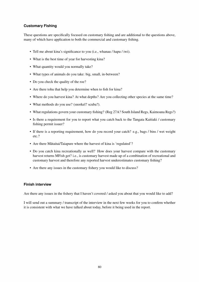
Customary Fishing

These questions are specifically focused on customary fishing and are additional to the questions above,many of which have application to both the commercial and customary fishing.

• Tell me about kina’s significance to you (i.e., whanau / hapu / iwi).

• What is the best time of year for harvesting kina?

• What quantity would you normally take?

• What types of animals do you take: big, small, in-between?

• Do you check the quality of the roe?

• Are there tohu that help you determine when to fish for kina?

• Where do you harvest kina? At what depths? Are you collecting other species at the same time?

• What methods do you use? (snorkel? scuba?).

• What regulations govern your customary fishing? (Reg 27A? South Island Regs, Kaimoana Regs?)

• Is there a requirement for you to report what you catch back to the Tangata Kaitiaki / customaryfishing permit issuer?

• If there is a reporting requirement, how do you record your catch? e.g., bags / bins / wet weightetc.?

• Are there Mataitai/Taiapure where the harvest of kina is ‘regulated’?

• Do you catch kina recreationally as well? How does your harvest compare with the customaryharvest returns MFish get? i.e., is customary harvest made up of a combination of recreational andcustomary harvest and therefore any reported harvest underestimates customary fishing?

• Are there any issues in the customary fishery you would like to discuss?

Finish interview

Are there any issues in the fishery that I haven’t covered / asked you about that you would like to add?

I will send out a summary / transcript of the interview in the next few weeks for you to confirm whetherit is consistent with what we have talked about today, before it being used in the report.

80

APPENDIX B: SAMPLE INTERVIEW TRANSCRIPT

Personal fishing history

Current role in the fishery. Kina quota owner, leases kina ACE, and kina fisher. Also fishes paua (ownsquota, and also leases ACE). Also had own factory to process kina up until a couple of years ago.

Length of time in fishery. 1991 onwards (initially as boat boy, and then diver). Aims to be involved in thekina fishery long-term.

Fishing strategy

Fishing location. Mainly fishes Stewart Island – Codfish to Big South Cape as these areas have betterrecovery than others.

Fishing methods. Hand-gather while free-diving (dredging has really only been used in the MarlboroughSounds).

Depth range covered. 0 – 40 feet

Number of people on fishing trip. 3 divers and dinghy boy

Return to same places? Yes, but an area needs around 3 years break from being fished so fish a 3 yearrotational harvest strategy. Although, tonnage greenweight will be low when we return to a previouslyfished spot, recoveries are better.

Catch

Amount caught on a daily basis. 1500 kg for a day trip using a 32 foot aluminium boat, and 5 tonne ifusing 40 foot fibreglass hull boat (steam out overnight then return the next night).

Kina size and row quality

Size limits? The best size kina to harvest is around the size of a grapefruit – this is an intermediate sizeand has better roe recovery than smaller sized, or larger sized kina. For the markets in Asia, smaller kinaare more desirable.

Where/when is roe recovery checked? Roe recovery is checked underwater. Kina get cracked open onthe bottom. If UBA could be used as a harvest method in the kina fishery, it would be easier to check roerecovery.

Roe quality. The best quality roe is found between October and February but then roe recovery dropsbetween February and June. However, from July onwards, kina fatten up again.

If there’s a bit of current and fewer kina, the roe is of better quality. For example, the middle of FoveauxStrait can get recoveries up to 17%.

You can fish down dense patches of kina and they come back with better recoveries - for example a

81

5% recovery area can be fished down to yield an 11% recovery from the same area the following year,although there will be fewer kina to harvest.

Indicators for kina roe quality? At the start of winter kina go skinny and then in spring they fatten upagain.

Storage/handling characteristics

Length of fishing trip. Day trips

Storage of kina on boat. They get taken to the dinghy to hold and get covered by hessian sugar sacks.The kina don’t get washed down as it can stress them. Ideally, it would be good to hold the kina live intanks.

Handling characteristics. Catch in hand nets using a rake.

Monitoring and reporting

Fine-scale reporting. Need to use only one book and report catch fine-scale (as the paua industry arealready doing).

Dataloggers as used by the paua divers. Yes, the kina association are talking about using dataloggers.

Processing

All kina landed is processed. When Fisher B was processing himself, he made sure kina were processedwithin 50 hours maximum from taking them out of the water.

Market and value

Market. Three years ago it was difficult to get enough kina for the markets.

Roe quality and price. If the supply of kina was consistent, it would fetch a higher price, For export, aconsistent supply is vital.

The money for kina can be as good as for paua. There are different grades of kina roe – 1, 2, 3, and 4.

When Fisher operated the factory, he would get $3 kg greenweight (half of this would go towards staff inthe factory, the other half to running the boat). The average price for kina greenweight would be around$1.90 per kilo throughout the season.

A few years back kina quota sold for $15 per kilo but now it’s down to $12 per kilo greenweight.

Divers paid on greenweight while factory workers paid a set hourly rate.

Yellow kina would be sold for $9.00 per kg wholesale and black kina for $7.50 per kg wholesale.

82

Marketing strategy. Kina area reasonably easy to market, and there is only so much kina the market canhandle. When he was processing kina, Fisher would make sales trips to build markets. Marketing SUR5kina is more difficult when the more sought after Chatham Islands kina is on the market.

Suggested changes to fishing practices?

Use of UBA. There is no selectivity at present with commercial free-diving for kina so we end up strippingareas of kina. Note that hookah is used in Tasmania for both abalone and urchins.

UBA would allow access to deeper stocks (such as those in Foveaux Strait). UBA would allow forselectivity and increase the value of the product. We would be better able to check roe recoveryunderwater.

Being able to use UBA would also help with providing consistent supply of kina to the market as fisherswould be able to dive on crappier days, although smaller boats still need good weather to go out. UBAwould also help to keep paua numbers up by stopping kina from taking over areas. Harvesting kinawould help maintain a balance between paua and kina numbers.

Harvest strategy

Limitations for harvest strategy. There is no time to be selective when free-diving due to limited bottom-time.

How do you harvest an area? Everything at in area is taken.

Other issues

Role of kina in the ecosystem. If paua are removed from a spot (for example, Dusky Sound), the kinacome in and take over.

83

APPENDIX C: SUMMARY OF KINA CATCH AND EFFORT DATA

The following pages contain a summary of commercial kina catch and effort data in each of the kinaquota management areas. Data are given for the 1990 to 2009 fishing years. The data are restricted tofishing that targeted kina, and that reported the primary method as either diving or hand-gathering, ordredging.

The pages for the dive fisheries are given in decreasing order of catch in the 2009 fishing year (SUR 5,SUR 4, SUR 7A, SUR 1B, SUR 1A, SUR 2A, SUR 2B, SUR9, and SUR 3). The pages for the dredgefisheries are given in decreasing order of average annual catch across the 1990 to 2009 fishing years(SUR 7A and SUR 1B).

There has been kina fishing in other QMAs; however, in the other areas there were never more than threevessels fishing in any given year. In order to meet Ministry of Fisheries data confidentiality requirements,data from these areas are not shown.

84

C.1 Southland (SUR 5) dive fishery

Table C-1: Summary of annual kina fishing effort and catch, from dive fishing. Catch is estimated (CELR)and landed greenweight, days is the number of diver days fished, vessels is the number of vessels fishing,and the raw CPUE is calculated by dividing the estimated greenweight by the number of diver days.

Fishing yearGreen weight (tonnes)

Days VesselsRaw CPUE

Estimated Landed (kg per diver day)

1989–90 11.3 15.4 66 12 171.71990–91 114.5 113.5 264 24 433.51991–92 219.8 241.7 558 41 393.91992–93 335.2 336.1 562 47 596.51993–94 293.5 292.5 665 36 441.31994–95 252.3 305.4 395 32 638.81995–96 183.9 240.2 297 24 619.11996–97 87.6 104.3 204 20 429.21997–98 72.6 124.1 115 16 630.91998–99 28.6 66.5 79 14 362.31999–00 8 11.7 30 6 265.02000–01 22.2 33.6 67 7 331.92001–02 111.8 121.6 177 12 631.92002–03 129.8 148.9 171 15 759.32003–04 187.5 210.6 216 8 868.22004–05 335.3 405 308 7 1088.82005–06 463.3 490.2 441 6 1050.52006–07 411.1 424.1 353 4 1164.62007–08 284.8 293.1 267 5 1066.62008–09 298.3 309 345 6 864.6

(a) Annual catch

0

100

200

300

400

500

Ann

ual c

atch

(to

nnes

)

90 92 94 96 98 00 02 04 06 08Fishing year

TACCEstimatedLanded

(b) Raw CPUE

●

●●

●

●

● ●

●

●

●

●

●

●

●

●

●●

●

●

●

Raw

CP

UE

(kg

per

div

er d

ay)

0

200

400

600

800

1000

1200

90 92 94 96 98 00 02 04 06 08Fishing year

(c) Average monthly catch

0

10

20

30

40

Cat

ch (

tonn

es)

O N D J F M A M J J A SMonth

Before QMSAfter QMS

(d) Average annual catch by statistical area

0

50

100

150

200

Cat

ch (

tonn

es)

030 029 027 025 031 032 028Statistical area

Before QMSAfter QMS

Figure C-1: Summary of kina catch data and effort data. (a) Annual catch history (b) Raw CPUE(c) Monthly catch (d) Average catch by statistical area. In (a) comparison is made between estimatedgreenweight and landed greenweight. In (b), (c), and (d) the estimated greenweight is used. In (c) and(d) comparison is made between fishing before and after the introduction of kina into the QMS.

85

C.2 Chatham Islands (SUR 4) dive fishery

Table C-2: Summary of annual kina fishing effort and catch, from dive fishing. Catch is estimated (CELR)and landed greenweight, days is the number of diver days fished, vessels is the number of vessels fishing,and the raw CPUE is calculated by dividing the estimated greenweight by the number of diver days.

Fishing yearGreen weight (tonnes)

Days VesselsRaw CPUE

Estimated Landed (kg per diver day)

1989–90 205.7 198.9 413 32 498.21990–91 49.4 54.8 164 18 301.41991–92 189.8 231.2 564 22 336.61992–93 21 23 67 8 313.01993–94 55.4 66 219 11 252.91994–95 59.7 159.9 119 16 501.81995–96 60.8 78.2 161 15 377.91996–97 214.8 229.9 415 25 517.61997–98 296 338.4 500 20 592.01998–99 181.2 210.7 387 17 468.31999–00 306.8 348.2 556 21 551.82000–01 458.1 629.2 610 23 750.92001–02 348.1 355.9 456 23 763.42002–03 166.6 171 257 18 648.42003–04 104.9 111.2 184 15 570.32004–05 86.4 92 146 9 591.82005–06 66.3 69.2 108 6 613.92006–07 111 112.9 194 15 572.32007–08 149.1 154 236 17 631.72008–09 133.1 134 202 16 659.0

(a) Annual catch

0

100

200

300

400

500

600

700

Ann

ual c

atch

(to

nnes

)

90 92 94 96 98 00 02 04 06 08Fishing year

TACCEstimatedLanded

(b) Raw CPUE

●

●●

●

●

●

●

●

●

●

●

● ●

●

●●

●

●

●●

Raw

CP

UE

(kg

per

div

er d

ay)

0

200

400

600

90 92 94 96 98 00 02 04 06 08Fishing year

(c) Average monthly catch

0

10

20

30

40

Cat

ch (

tonn

es)

O N D J F M A M J J A SMonth

Before QMSAfter QMS

(d) Average annual catch by statistical area

0

20

40

60

80

100

120

Cat

ch (

tonn

es)

49 51 50 52Statistical area

Before QMSAfter QMS

Figure C-2: Summary of kina catch data and effort data. (a) Annual catch history (b) Raw CPUE(c) Monthly catch (d) Average catch by statistical area. In (a) comparison is made between estimatedgreenweight and landed greenweight. In (b), (c), and (d) the estimated greenweight is used. In (c) and(d) comparison is made between fishing before and after the introduction of kina into the QMS.

86

C.3 Nelson Marlborough (SUR 7A) dive fishery

Table C-3: Summary of annual kina fishing effort and catch, from dive fishing. Catch is estimated (CELR)and landed greenweight, days is the number of diver days fished, vessels is the number of vessels fishing,and the raw CPUE is calculated by dividing the estimated greenweight by the number of diver days.

Fishing yearGreen weight (tonnes)

Days VesselsRaw CPUE

Estimated Landed (kg per diver day)

1989–90 30.1 33.1 158 11 190.41990–91 31.6 39.5 217 15 145.61991–92 96.3 111.8 600 20 160.51992–93 150.7 155.7 580 25 259.81993–94 85.4 91.3 420 22 203.41994–95 114.3 107.7 576 22 198.51995–96 62.2 98 259 10 240.11996–97 38.6 42.3 160 11 241.51997–98 59.3 58 216 18 274.41998–99 50 61.3 248 13 201.61999–00 28.7 37 147 7 195.32000–01 46.4 52.7 207 11 224.22001–02 42.6 41 144 12 295.82002–03 62.8 64.8 197 10 319.02003–04 83.6 85.5 191 7 437.62004–05 62.1 62 110 7 564.92005–06 61.4 63.7 126 11 487.52006–07 93.8 100.7 243 15 386.12007–08 122.3 130.4 252 13 485.22008–09 130.9 132.9 322 15 406.4

(a) Annual catch

0

50

100

150

Ann

ual c

atch

(to

nnes

)

90 92 94 96 98 00 02 04 06 08Fishing year

TACCEstimatedLanded

(b) Raw CPUE

●

●●

●

● ●

● ●

●

● ●●

●●

●

●

●

●

●

●

Raw

CP

UE

(kg

per

div

er d

ay)

0

100

200

300

400

500

90 92 94 96 98 00 02 04 06 08Fishing year

(c) Average monthly catch

0

5

10

15

Cat

ch (

tonn

es)

O N D J F M A M J J A SMonth

Before QMSAfter QMS

(d) Average annual catch by statistical area

0

20

40

60

80

Cat

ch (

tonn

es)

17 38 18 36Statistical area

Before QMSAfter QMS

Figure C-3: Summary of kina catch data and effort data. (a) Annual catch history (b) Raw CPUE(c) Monthly catch (d) Average catch by statistical area. In (a) comparison is made between estimatedgreenweight and landed greenweight. In (b), (c), and (d) the estimated greenweight is used. In (c) and(d) comparison is made between fishing before and after the introduction of kina into the QMS.

87

C.4 Hauraki Gulf and Bay of Plenty (SUR 1B) dive fishery

Table C-4: Summary of annual kina fishing effort and catch, from dive fishing. Catch is estimated (CELR)and landed greenweight, days is the number of diver days fished, vessels is the number of vessels fishing,and the raw CPUE is calculated by dividing the estimated greenweight by the number of diver days.

Fishing yearGreen weight (tonnes)

Days VesselsRaw CPUE

Estimated Landed (kg per diver day)

1989–90 11.1 18.8 105 6 105.41990–91 36.2 37.8 216 16 167.51991–92 66.8 70.3 514 18 129.91992–93 51.2 62.2 345 21 148.51993–94 116.1 138.6 747 23 155.41994–95 200.3 229.1 874 21 229.21995–96 199.1 240.6 886 15 224.71996–97 152.1 159.3 811 14 187.51997–98 152.5 139 743 12 205.21998–99 238.6 243.6 911 13 261.91999–00 236.2 244.1 1 029 13 229.62000–01 205.1 225.5 801 11 256.12001–02 227.3 244.9 815 9 278.82002–03 210.8 220.9 930 6 226.62003–04 111.7 119.2 508 10 219.82004–05 119.9 131 475 9 252.42005–06 138.6 160.1 703 9 197.22006–07 143.6 154.2 542 7 265.02007–08 122.4 132.9 427 5 286.72008–09 121.6 138.9 493 7 246.6

(a) Annual catch

0

50

100

150

200

250

Ann

ual c

atch

(to

nnes

)

90 92 94 96 98 00 02 04 06 08Fishing year

TACCEstimatedLanded

(b) Raw CPUE

●

●

●

●●

● ●

●

●

●

●

●

●

●●

●

●

●

●

●

Raw

CP

UE

(kg

per

div

er d

ay)

0

50

100

150

200

250

90 92 94 96 98 00 02 04 06 08Fishing year

(c) Average monthly catch

0

5

10

15

20

25

Cat

ch (

tonn

es)

O N D J F M A M J J A SMonth

Before QMSAfter QMS

(d) Average annual catch by statistical area

0

20

40

60

80

100

Cat

ch (

tonn

es)

008 007 005 006 009 010 003 004 907Statistical area

Before QMSAfter QMS

Figure C-4: Summary of kina catch data and effort data. (a) Annual catch history (b) Raw CPUE(c) Monthly catch (d) Average catch by statistical area. In (a) comparison is made between estimatedgreenweight and landed greenweight. In (b), (c), and (d) the estimated greenweight is used. In (c) and(d) comparison is made between fishing before and after the introduction of kina into the QMS.

88

C.5 East Northland (SUR 1A) dive fishery

Table C-5: Summary of annual kina fishing effort and catch, from dive fishing. Catch is estimated (CELR)and landed greenweight, days is the number of diver days fished, vessels is the number of vessels fishing,and the raw CPUE is calculated by dividing the estimated greenweight by the number of diver days.

Fishing yearGreen weight (tonnes)

Days VesselsRaw CPUE

Estimated Landed (kg per diver day)

1989–90 1.4 2.7 16 3 90.41990–91 20.7 22.2 110 8 187.91991–92 20.2 22 136 9 148.31992–93 13.1 15.1 79 8 166.31993–94 8.3 23.9 70 10 118.11994–95 12.2 20.7 83 11 147.41995–96 19.6 59.1 185 8 106.11996–97 10.9 12.7 104 5 104.41997–98 11.7 10.8 164 6 71.61998–99 16.7 55 210 7 79.51999–00 42.1 46.9 224 8 188.02000–01 10.9 17.6 55 4 198.92001–02 37.9 47.5 161 4 235.42002–03 15.9 20.4 73 4 217.82003–04 26.7 27.3 79 4 337.82004–05 21.3 23 68 6 313.52005–06 40.5 44.2 271 4 149.42006–07 39.8 43.3 244 7 163.02007–08 32.7 39.5 181 6 180.62008–09 24.8 31.7 87 4 285.5

(a) Annual catch

0

10

20

30

40

50

60

70

Ann

ual c

atch

(to

nnes

)

90 92 94 96 98 00 02 04 06 08Fishing year

TACCEstimatedLanded

(b) Raw CPUE

●

●

●●

●

●

● ●

●●

●●

●●

●

●

●●

●

●

Raw

CP

UE

(kg

per

div

er d

ay)

0

50

100

150

200

250

300

350

90 92 94 96 98 00 02 04 06 08Fishing year

(c) Average monthly catch

0

1

2

3

4

5

6

Cat

ch (

tonn

es)

O N D J F M A M J J A SMonth

Before QMSAfter QMS

(d) Average annual catch by statistical area

0

5

10

15

20

25

Cat

ch (

tonn

es)

003 002 001 005Statistical area

Before QMSAfter QMS

Figure C-5: Summary of kina catch data and effort data. (a) Annual catch history (b) Raw CPUE(c) Monthly catch (d) Average catch by statistical area. In (a) comparison is made between estimatedgreenweight and landed greenweight. In (b), (c), and (d) the estimated greenweight is used. In (c) and(d) comparison is made between fishing before and after the introduction of kina into the QMS.

89

C.6 East Coast (SUR 2A) dive fishery

Table C-6: Summary of annual kina fishing effort and catch, from dive fishing. Catch is estimated (CELR)and landed greenweight, days is the number of diver days fished, vessels is the number of vessels fishing,and the raw CPUE is calculated by dividing the estimated greenweight by the number of diver days.

Fishing yearGreen weight (tonnes)

Days VesselsRaw CPUE

Estimated Landed (kg per diver day)

1989–90 291.4 283.3 862 8 338.01990–91 89.7 90.2 292 7 307.31991–92 35.8 36.2 194 4 184.31992–93 166.5 165.9 570 9 292.11993–94 181.2 174.8 660 8 274.51994–95 130.9 129.2 457 5 286.51995–96 43.6 41.8 172 4 253.61996–97 - - - 2 -1997–98 - - - 1 -1998–99 - - - 1 -1999–00 - - - 2 -2000–01 4.7 5.6 28 3 166.42001–02 - - - 1 -2002–03 - - - 2 -2003–04 14.5 14.7 52 3 279.32004–05 6.7 6.7 36 4 186.02005–06 21.9 22.6 81 6 270.52006–07 16.3 16.6 59 6 276.82007–08 19.5 19.7 58 6 335.52008–09 19.1 20.1 63 4 302.9

(a) Annual catch

0

50

100

150

200

250

300

Ann

ual c

atch

(to

nnes

)

90 92 94 96 98 00 02 04 06 08Fishing year

TACCEstimatedLanded

(b) Raw CPUE●

●

●

●●

●

●

●

●

●

● ●

●

●

Raw

CP

UE

(kg

per

div

er d

ay)

0

50

100

150

200

250

300

350

90 92 94 96 98 00 02 04 06 08Fishing year

(c) Average monthly catch

0

5

10

15

Cat

ch (

tonn

es)

O N D J F M A M J J A SMonth

Before QMSAfter QMS

(d) Average annual catch by statistical area

0

20

40

60

80

Cat

ch (

tonn

es)

13 11 12Statistical area

Before QMSAfter QMS

Figure C-6: Summary of kina catch data and effort data. (a) Annual catch history (b) Raw CPUE(c) Monthly catch (d) Average catch by statistical area. In (a) comparison is made between estimatedgreenweight and landed greenweight. In (b), (c), and (d) the estimated greenweight is used. In (c) and(d) comparison is made between fishing before and after the introduction of kina into the QMS.

90

C.7 Wairarapa and Wellington (SUR 2B) dive fishery

Table C-7: Summary of annual kina fishing effort and catch, from dive fishing. Catch is estimated (CELR)and landed greenweight, days is the number of diver days fished, vessels is the number of vessels fishing,and the raw CPUE is calculated by dividing the estimated greenweight by the number of diver days.

Fishing yearGreen weight (tonnes)

Days VesselsRaw CPUE

Estimated Landed (kg per diver day)

1989–90 - - - 1 -1990–91 - - - 2 -1991–92 - - - 1 -1992–93 3.5 4.3 31 4 111.81993–94 2.7 2.8 15 3 178.71994–95 - - - 0 -1995–961996–971997–981998–991999–00 - - - 1 -2000–01 7.1 8.8 20 3 357.02001–02 1.8 1.5 7 3 255.72002–03 - - - 2 -2003–04 - - - 2 -2004–05 - - - 2 -2005–06 - - - 2 -2006–07 11.9 11.1 27 3 439.12007–08 0.2 0.2 3 3 83.32008–09 - - - 1 -

(a) Annual catch

0

5

10

15

20

25

30

35

Ann

ual c

atch

(to

nnes

)

90 92 94 96 98 00 02 04 06 08Fishing year

TACCEstimatedLanded

(b) Raw CPUE

●

●

●

●

●

●

Raw

CP

UE

(kg

per

div

er d

ay)

0

100

200

300

400

90 92 94 96 98 00 02 04 06 08Fishing year

(c) Average monthly catch

0.0

0.5

1.0

1.5

2.0

2.5

Cat

ch (

tonn

es)

O N D J F M A M J J A SMonth

Before QMSAfter QMS

(d) Average annual catch by statistical area

0

1

2

3

4

5

Cat

ch (

tonn

es)

16 15Statistical area

Before QMSAfter QMS

Figure C-7: Summary of kina catch data and effort data. (a) Annual catch history (b) Raw CPUE(c) Monthly catch (d) Average catch by statistical area. In (a) comparison is made between estimatedgreenweight and landed greenweight. In (b), (c), and (d) the estimated greenweight is used. In (c) and(d) comparison is made between fishing before and after the introduction of kina into the QMS.

91

C.8 West Auckland (SUR 9) dive fishery

Table C-8: Summary of annual kina fishing effort and catch, from dive fishing. Catch is estimated (CELR)and landed greenweight, days is the number of diver days fished, vessels is the number of vessels fishing,and the raw CPUE is calculated by dividing the estimated greenweight by the number of diver days.

Fishing yearGreen weight (tonnes)

Days VesselsRaw CPUE

Estimated Landed (kg per diver day)

1989–90 - - - 1 -1990–91 - - - 1 -1991–92 - - - 1 -1992–93 - - - 1 -1993–941994–95 0.4 0.5 6 3 69.21995–96 - - - 2 -1996–97 2.7 2.8 8 3 337.51997–98 1.1 3.2 10 3 107.21998–99 1.9 3.4 10 3 185.01999–00 5.4 6.9 14 5 383.32000–01 - - - 1 -2001–02 1.4 4.5 9 3 156.62002–032003–04 - - - 2 -2004–05 - - - 1 -2005–06 - - - 1 -2006–07 1.4 4.9 18 4 76.02007–08 - - - 1 -2008–09 2.5 2.7 9 3 274.6

(a) Annual catch

0

2

4

6

8

10

12

Ann

ual c

atch

(to

nnes

)

90 92 94 96 98 00 02 04 06 08Fishing year

TACCEstimatedLanded

(b) Raw CPUE

●

●

●

●

●

●

●

●

Raw

CP

UE

(kg

per

div

er d

ay)

0

100

200

300

90 92 94 96 98 00 02 04 06 08Fishing year

(c) Average monthly catch

0.0

0.1

0.2

0.3

0.4

Cat

ch (

tonn

es)

O N D J F M A M J J A SMonth

Before QMSAfter QMS

(d) Average annual catch by statistical area

0.0

0.1

0.2

0.3

0.4

0.5

0.6

0.7

Cat

ch (

tonn

es)

47 45 44 48 42 43Statistical area

Before QMSAfter QMS

Figure C-8: Summary of kina catch data and effort data. (a) Annual catch history (b) Raw CPUE(c) Monthly catch (d) Average catch by statistical area. In (a) comparison is made between estimatedgreenweight and landed greenweight. In (b), (c), and (d) the estimated greenweight is used. In (c) and(d) comparison is made between fishing before and after the introduction of kina into the QMS.

92

C.9 Canterbury and Otago (SUR 3) dive fishery

Table C-9: Summary of annual kina fishing effort and catch, from dive fishing. Catch is estimated (CELR)and landed greenweight, days is the number of diver days fished, vessels is the number of vessels fishing,and the raw CPUE is calculated by dividing the estimated greenweight by the number of diver days.

Fishing yearGreen weight (tonnes)

Days VesselsRaw CPUE

Estimated Landed (kg per diver day)

1989–90 1.3 1.9 17 5 75.31990–91 8 9.8 60 7 132.71991–92 6.5 9 46 7 141.71992–93 21.7 23.2 125 14 173.41993–94 5.6 5.9 52 10 107.21994–95 6.3 10.4 58 8 108.21995–96 3.6 0.4 13 5 273.61996–97 25 27.1 43 6 582.01997–98 - - - 2 -1998–99 - - - 1 -1999–00 8 8.9 17 4 470.62000–01 15.5 15.7 57 4 272.62001–02 4.6 5 28 4 163.12002–03 - - - 2 -2003–04 - - - 1 -2004–05 - - - 1 -2005–06 - - - 1 -2006–07 7.1 29.7 32 6 221.42007–08 1.4 1.6 30 4 47.22008–09 9.1 9.2 63 4 144.0

(a) Annual catch

0

5

10

15

20

25

30

35

Ann

ual c

atch

(to

nnes

)

90 92 94 96 98 00 02 04 06 08Fishing year

TACCEstimatedLanded

(b) Raw CPUE

●

● ●

●

● ●

●

●

●

●

●

●

●

●

Raw

CP

UE

(kg

per

div

er d

ay)

0

100

200

300

400

500

600

90 92 94 96 98 00 02 04 06 08Fishing year

(c) Average monthly catch

0.0

0.5

1.0

1.5

2.0

2.5

Cat

ch (

tonn

es)

O N D J F M A M J J A SMonth

Before QMSAfter QMS

(d) Average annual catch by statistical area

0

1

2

3

4

5

6

Cat

ch (

tonn

es)

18 24 26 23 303Statistical area

Before QMSAfter QMS

Figure C-9: Summary of kina catch data and effort data. (a) Annual catch history (b) Raw CPUE(c) Monthly catch (d) Average catch by statistical area. In (a) comparison is made between estimatedgreenweight and landed greenweight. In (b), (c), and (d) the estimated greenweight is used. In (c) and(d) comparison is made between fishing before and after the introduction of kina into the QMS.

93

C.10 Nelson Marlborough (SUR 7A) dredge fishery

Table C-10: Summary of annual kina fishing effort and catch, from dredge fishing. Catch is estimated(CELR) and landed greenweight, hours is the total number of hours dredged, vessels is the number ofvessels fishing, and the raw CPUE is calculated by dividing the estimated greenweight by the hours fished.

Fishing yearGreen weight (tonnes)

Hours VesselsRaw CPUE

Estimated Landed (kg per hour)

1989–90 10.1 10.3 185 1 54.61990–91 24 27.1 342 2 70.11991–92 7.1 9.4 223 3 31.71992–93 48 42.2 494 2 97.11993–94 6.7 10.1 140 3 47.81994–95 28.4 36.2 342 2 83.21995–96 64.1 77.7 1 103 1 58.11996–97 50.8 73.1 1 163 1 43.71997–98 81.1 89.6 1 992 2 40.61998–99 62.1 62.9 1 939 1 32.01999–00 27.4 26.8 782 2 35.12000–01 26 23.3 530 1 49.12001–02 1.1 3.2 39 2 29.72002–03 0.3 0.3 15 1 21.32003–04 0.2 1.9 3 1 73.22004–05 27.4 34.1 319 6 85.92005–06 8.1 11.8 131 4 61.82006–07 - - - 1 -2007–08 - - - 1 -2008–09 - - - 1 -

(a) Annual catch

0

50

100

150

Ann

ual c

atch

(to

nnes

)

90 92 94 96 98 00 02 04 06 08Fishing year

TACCEstimatedLanded

(b) Raw CPUE

●

●

●

●

●

●

●

●●

●●

●

●

●

●

●

●

Raw

CP

UE

(kg

per

hou

r)

020

4060

8010

0

90 92 94 96 98 00 02 04 06 08Fishing year

(c) Average monthly catch

0

1

2

3

4

5

Cat

ch (

tonn

es)

O N D J F M A M J J A SMonth

Before QMSAfter QMS

(d) Average annual catch by statistical area

0

10

20

30

40

Cat

ch (

tonn

es)

17Statistical area

Before QMSAfter QMS

Figure C-10: Summary of kina catch data and effort data. (a) Annual catch history (b) Raw CPUE (c)Monthly catch (d) Catch by statistical area. In (a) comparison is made between estimated greenweight andlanded greenweight. In (b), (c), and (d) the estimated greenweight is used. In (b) and (c) comparison is madebetween fishing before and after the introduction of kina into the QMS.

94

C.11 Hauraki Gulf and Bay of Plenty (SUR 1B) dredge fishery

Table C-11: Summary of annual kina fishing effort and catch, from dredge fishing. Catch is estimated(CELR) and landed greenweight, hours is the total number of hours dredged, vessels is the number ofvessels fishing, and the raw CPUE is calculated by dividing the estimated greenweight by the hours fished.

Fishing yearGreen weight (tonnes)

Hours VesselsRaw CPUE

Estimated Landed (kg per hour)

1989–901990–91 0.4 1.3 12 1 38.31991–92 0.7 4 1 175.01992–93 0.1 0.1 4 1 26.71993–94 1.5 1.8 22 1 67.51994–951995–961996–971997–98 3.5 1.2 36 1 97.51998–99 17.1 3.7 284 1 59.91999–002000–01 0.3 0.5 8 1 43.82001–022002–032003–042004–052005–062006–07 - - - 1 -2007–08 - - - 1 -2008–09

(a) Annual catch

0

50

100

150

Ann

ual c

atch

(to

nnes

)

90 92 94 96 98 00 02 04 06 08Fishing year

TACCEstimatedLanded

(b) Raw CPUE

●

●

●

●

●

●

●

Raw

CP

UE

(kg

per

hou

r)

050

100

150

90 92 94 96 98 00 02 04 06 08Fishing year

(c) Average monthly catch

0.0

0.1

0.2

0.3

0.4

0.5

0.6

Cat

ch (

tonn

es)

O N D J F M A M J J A SMonth

(d) Average annual catch by statistical area

0.0

0.5

1.0

1.5

Cat

ch (

tonn

es)

7Statistical area

Figure C-11: Summary of kina catch data and effort data. (a) Annual catch history (b) Raw CPUE (c)Monthly catch (d) Catch by statistical area. In (a) comparison is made between estimated greenweight andlanded greenweight. In (b), (c), and (d) the estimated greenweight is used.

95