1

Multiple Regression Analysis

y = 0 + 1x1 + 2x2 + . . . kxk + u

4. Further Issues

2

Redefining Variables

Changing the scale of the y variable will lead to a corresponding change in the scale of the coefficients and standard errors, so no change in the significance or interpretation

Changing the scale of one x variable will lead to a change in the scale of that coefficient and standard error, so no change in the significance or interpretation

3

Beta Coefficients

Occasional you’ll see reference to a “standardized coefficient” or “beta coefficient” which has a specific meaning

Idea is to replace y and each x variable with a standardized version – i.e. subtract mean and divide by standard deviation

Coefficient reflects standard deviation of yfor a one standard deviation change in x

4

Functional Form

OLS can be used for relationships that are not strictly linear in x and y by using nonlinear functions of x and y – will still be linear in the parameters

Can take the natural log of x, y or both

Can use quadratic forms of x

Can use interactions of x variables

5

Interpretation of Log Models

If the model is ln(y) = 0 + 1ln(x) + u

1 is the elasticity of y with respect to x

If the model is ln(y) = 0 + 1x + u

1 is approximately the percentage change in y given a 1 unit change in x

If the model is y = 0 + 1ln(x) + u

1 is approximately the change in y for a 100 percent change in x

6

Why use log models?

Log models are invariant to the scale of the variables since measuring percent changes

They give a direct estimate of elasticity

For models with y > 0, the conditional distribution is often heteroskedastic or skewed, while ln(y) is much less so

The distribution of ln(y) is more narrow, limiting the effect of outliers

7

Some Rules of Thumb

What types of variables are often used in log form?

Dollar amounts that must be positive

Very large variables, such as population

What types of variables are often used in level form?

Variables measured in years

Variables that are a proportion or percent

8

Quadratic Models

For a model of the form y = 0 + 1x + 2x2 + u

we can’t interpret 1 alone as measuring the change in y with respect to x, we need to take into account 2 as well, since

x

x

y

xxy

21

21

ˆ2ˆˆ

so ,ˆ2ˆˆ

9

More on Quadratic Models

Suppose that the coefficient on x is positive and the coefficient on x2 is negative

Then y is increasing in x at first, but will eventually turn around and be decreasing in x

21*

21

ˆ2ˆat be will

point turning the0ˆ and 0ˆFor

x

10

More on Quadratic Models

Suppose that the coefficient on x is negative and the coefficient on x2 is positive

Then y is decreasing in x at first, but will eventually turn around and be increasing in x

0ˆ and 0ˆ when as same the

is which ,ˆ2ˆat be will

point turning the0ˆ and 0ˆFor

21

21*

21

x

11

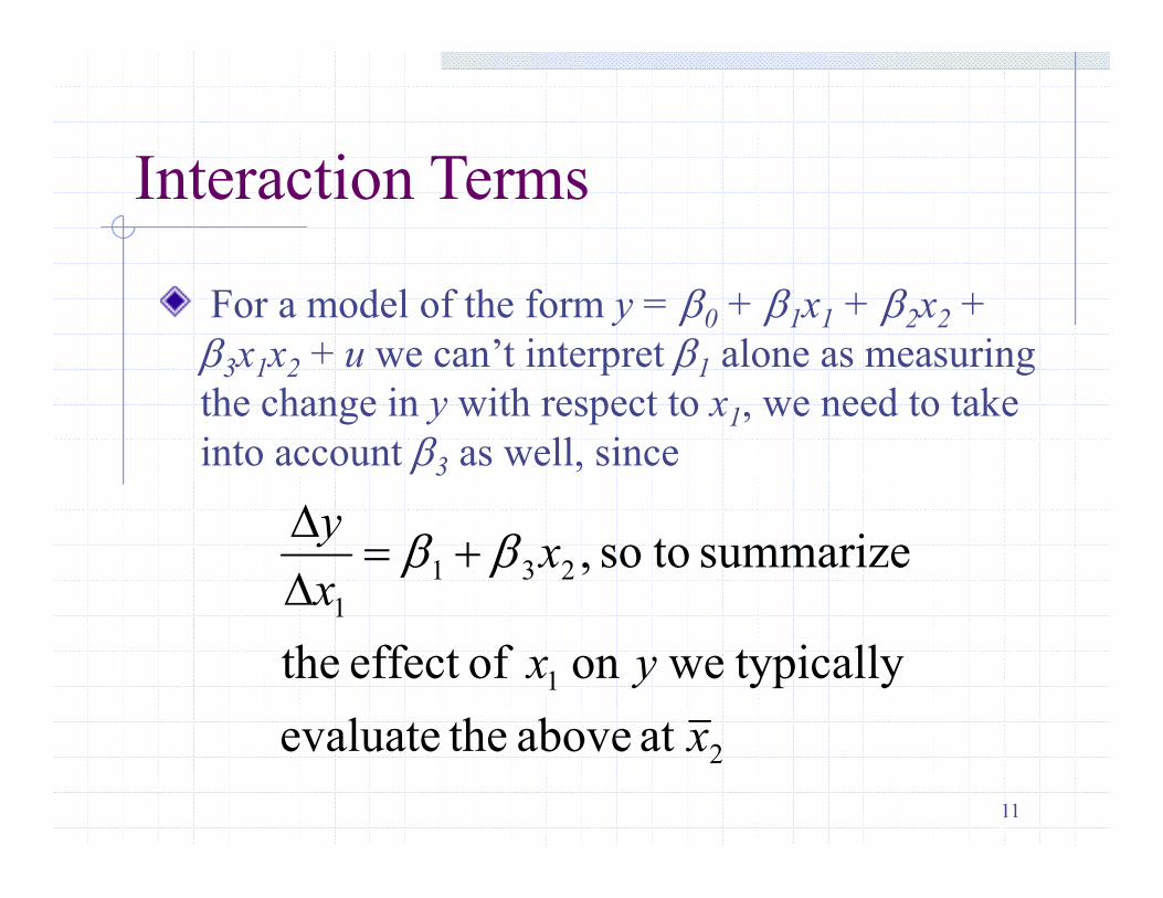
Interaction Terms

For a model of the form y = 0 + 1x1 + 2x2 + 3x1x2 + u we can’t interpret 1 alone as measuring the change in y with respect to x1, we need to take into account 3 as well, since

2

1

231

1

at above theevaluate

typically weon ofeffect the

summarize toso ,

x

yx

xx

y

12

Adjusted R-Squared

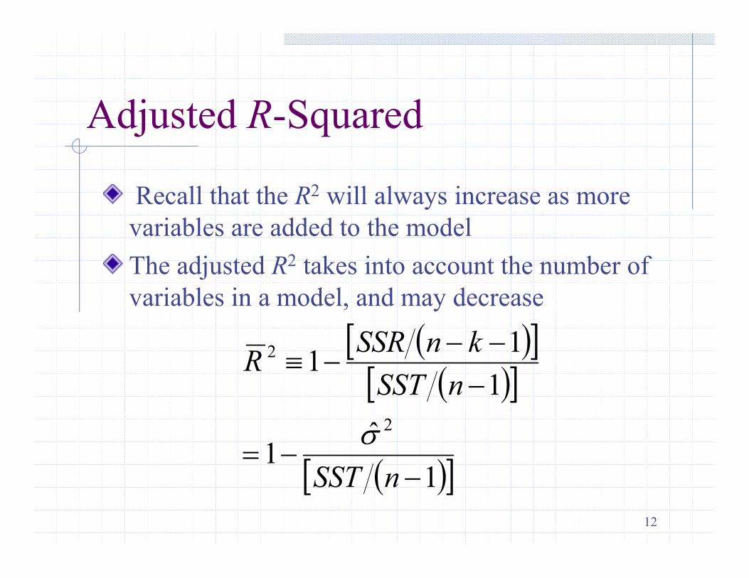
Recall that the R2 will always increase as more variables are added to the model

The adjusted R2 takes into account the number of variables in a model, and may decrease

1

ˆ1

1

11

2

2

nSST

nSST

knSSRR

13

Adjusted R-Squared (cont)

It’s easy to see that the adjusted R2 is just (1 – R2)(n – 1) / (n – k – 1), but most packages will give you both R2 and adj-R2

You can compare the fit of 2 models (with the same y) by comparing the adj-R2

You cannot use the adj-R2 to compare models with different y’s (e.g. y vs. ln(y))

14

Goodness of Fit

Important not to fixate too much on adj-R2

and lose sight of theory and common sense

If economic theory clearly predicts a variable belongs, generally leave it in

Don’t want to include a variable that prohibits a sensible interpretation of the variable of interest – remember ceteris paribus interpretation of multiple regression

15

Standard Errors for Predictions

Suppose we want to use our estimates to obtain a specific prediction?

First, suppose that we want an estimate of E(y|x1=c1,…xk=ck) = q0 = 0+1c1+ …+ kck

This is easy to obtain by substituting the x’s in our estimated model with c’s , but what about a standard error?

Really just a test of a linear combination

16

Predictions (cont)

Can rewrite as 0 = q0 – 1c1 – … – kck

Substitute in to obtain y = q0 + 1 (x1 - c1) + … + k (xk - ck) + u

So, if you regress yi on (xij - cij) the intercept will give the predicted value and its standard error

Note that the standard error will be smallest when the c’s equal the means of the x’s

17

Predictions (cont)

This standard error for the expected value is not the same as a standard error for an outcome on y

We need to also take into account the variance in the unobserved error. Let the prediction error be

21

220020

0000

0000

110000

ˆˆˆ so ,ˆ

ˆˆ and 0ˆ

ˆˆˆ

yseeseyVar

uVaryVareVareE

yuxxyye kk

18

Prediction interval

0025.

0

0

0001

00

ˆˆ

for interval prediction 95% a have we

ˆˆ given that so ,~ˆˆ

esety

y

yyetesee kn

Usually the estimate of s2 is much larger than the variance of the prediction, thus

This prediction interval will be a lot wider than the simple confidence interval for the prediction

19

Residual Analysis

Information can be obtained from looking at the residuals (i.e. predicted vs. observed)

Example: Regress price of cars on characteristics – big negative residuals indicate a good deal

Example: Regress average earnings for students from a school on student characteristics – big positive residuals indicate greatest value-added

20

Predicting y in a log model

Simple exponentiation of the predicted ln(y) will underestimate the expected value of y

Instead need to scale this up by an estimate of the expected value of exp(u)

yy

NuuE

n̂lexp2ˆexpˆ

follows asy predict can case In this

,0~ if )2exp()exp(

2

2

21

Predicting y in a log model

If u is not normal, E(exp(u)) must be estimated using an auxiliary regression

Create the exponentiation of the predicted ln(y), and regress y on it with no intercept

The coefficient on this variable is the estimate of E(exp(u)) that can be used to scale up the exponentiation of the predicted ln(y) to obtain the predicted y

22

Comparing log and level models

A by-product of the previous procedure is a method to compare a model in logs with one in levels.

Take the fitted values from the auxiliary regression, and find the sample correlation between this and y

Compare the R2 from the levels regression with this correlation squared