chapter03g - eigenvalue problems · above equation are known as eigenvalues and eigenfunctions...

EIGENVALUE PROBLEMS

Many of the techniques for solving two-dimensional time-dependent problems such as the diffusion and wave equations are very closely related to a corresponding boundary value problem.

In this section, we will investigate the relationship between the time-dependent problem and its corresponding boundary value problem.

Also we investigate how the FEM can be used to extract information about the eigenvalue and eigenfunctions of the corresponding boundary value problems.

EIGENVALUE PROBLEMS

Time-dependent diffusion problems can frequently be stated as:

2 , , , 0 inx y f x y tt

1

2

, on

, on

, ,0 ,

g s t

h s tnx y c x y

The first two auxiliary conditions are boundary conditions and the third an initial condition.

Such problems are frequently referred to as initial-boundary value problems.

EIGENVALUE PROBLEMS

The corresponding completely homogeneous boundary value problem, obtained by taking f = g = h = 0, is:

2 , 0 inx yt

1

2

0 on

0 onn

EIGENVALUE PROBLEMS

Solutions of this completely homogeneous boundary value problem have great utility in solving the original nonhomogeneous initial-boundary value problem.

For the diffusion problem, solutions of the homogeneous form of the time-depend diffusion equation are known generally to behave according to,

leading to:

, , , expx y t x y t

2 0 in

1

2

0 on

0 onn

where =

EIGENVALUE PROBLEMS

The 's and corresponding nontrivial 's that satisfy the above equation are known as eigenvalues and eigenfunctions respectively.

The words eigenvalue and eigenvector are derived from the German word "eigen" which means "proper" or "characteristic."

These are the two-dimensional counterparts of the n and un

discussed in one-dimensional eigenvalue problems.

2 0 in

1

2

0 on

0 onn

EIGENVALUE PROBLEMS

This differential equation is known as the Helmholtz Equationand occurs with remarkable frequency in mathematical models.

The problem to be solved is that of finding the eigenvalues and eigenfunctions satisfying the differential equation and boundary conditions for the two-dimensional region .

Exact solutions are known only for a few special regions .

2 0 in

1

2

0 on

0 onn

CIVL 7/8111 2-D Boundary Value Problems - Eigenvalue Problems 1/14

EIGENVALUE PROBLEMS

Hermann Ludwig Ferdinand von Helmholtz (August 31, 1821 –September 8, 1894) was a German physician and physicist who made significant contributions to several widely varied areas of modern science.

In physics, he is known for his theories on the conservation of energy, work in electrodynamics, chemical thermodynamics, and on a mechanical foundation of thermodynamics.

The largest German association of research institutions, the Helmholtz Association, is named after him.

EIGENVALUE PROBLEMS

In a completely similar fashion, the two-dimensional initial-boundary value problem associated with the scalar wave equation can be written as:

Here, the first two conditions are boundary conditions and the second two are initial conditions.

22 2

2, , 0 inc f x y t

t

1

2

, on

, on

, ,0 ,

, ,0,

g s t

s h s tn

x y c x y

x yd x y

t

EIGENVALUE PROBLEMS

Frequently, is a displacement or generalized displacement and hence /t is a velocity or generalized velocity.

For a physical problem associated with the wave equation it is usually appropriate to investigate solutions to the homogeneous differential equation and boundary conditions of the form,

again leading to:

where = (/c)2

, , , expx y t x y i t

2 0 in

1

2

0 on

0 onn

EIGENVALUE PROBLEMS

This is precisely the same completely homogeneous boundary value problem for the diffusion problem.

This equation describes a two-dimensional vibrating membrane, with the edges clamped to be motionless.

2 0 in

1

2

0 on

0 onn

Finite Element Models for the Helmholtz Equation

The finite element model for the Helmholtz equation will be discussed in terms of the typical region shown below.

EIGENVALUE PROBLEMS

1

0

on

2 0

in

1

2

2

0

onn

Discretization and interpolation are carried out in the same fashion as we have discussed earlier.


The Galerkin finite element method will be used to generate the desired algebraic equations for determining the approximate eigenvalues and eigenfunctions.

The form of the solution is taken as:

EIGENVALUE PROBLEMS

where the ni functions are appropriate nodally based inter-polation functions and i are the unknown values of (x, y).

1

, ,N

i ii

x y n x y



With the test function designated as , the appropriate weak form for this boundary value problem is:

EIGENVALUE PROBLEMS

Taking:

2

0dA ds dAx x y y

1

, ,N

i ii

x y n x y

, 1, 2, , yields:kn k N


With the previous substitutions, the boundary value problems becomes:

EIGENVALUE PROBLEMS

1

Nk i k i

ii

n n n ndA

x x y y

1

N

k i ii

n n dA

1, 2, ,k N

2

1

N

k i ii

n n ds

dAx x y y

2

ds

dA


With the previous substitutions, the boundary value problems becomes:

EIGENVALUE PROBLEMS

1

Nk i k i

ii

n n n ndA

x x y y

1

0N

k i ii

n n dA

1, 2, ,k N

2

1

N

k i ii

n n ds


These equations can be written in a more convenient form:

EIGENVALUE PROBLEMS

where:

1

0N

ki ki ii

K M 1, 2, ,k N

'e e

G G GK k a

A

dAx x y y

T T

e

N N N Nk

2e

ds

Tea N N

eA

dATem NN

e

G GM m


These equations can be written in a more convenient form:

EIGENVALUE PROBLEMS

The above equation is an example of the generalized linear algebraic eigenvalue problem.

The me is referred to as an elemental consistent mass matrix.

1

0N

ki ki ii

K M 1, 2, ,k N

This results in:

where the rows and columns associated with the constraints have been removed.


The boundary conditions for the Helmholtz equation are entirely homogeneous.

In particular, the constraints associated with the essential boundary conditions on 1 can be enforced by deleting the row and column corresponding to the degree of freedom in question.

EIGENVALUE PROBLEMS

0 * * * *G G G GK Ψ - M Ψ



The solution is obtained by determining the eigenvalues and corresponding eigenvectors.

For a problem with a small number (two to four) of constrained degrees of freedom, it is perhaps feasible to extract the eigen information by hand.

EIGENVALUE PROBLEMS

1 * *G GA K MThis results in:

where the rows and columns associated with the constraints have been removed.

0 * * * *G G G GK Ψ - M Ψ


For larger problems, it is essential to have a robust computer code for this task.

Appendix C in your textbook contains FORTRAN source listings for several routines that may be used in this regard.

More conveniently, you can use MathCAD’s eigenvector functions: eigenvals(A) and eigenvecs(A)

EIGENVALUE PROBLEMS

In MATLAB, the function [V,D] = eig(A) returns diagonal matrix D of eigenvalues and matrix V whose columns are the corresponding right eigenvectors.


EIGENVALUE PROBLEMS

The propagation of time harmonic sound waves is usually described by the Helmholtz equation.

When the pressure source is moving with respect to the fluid, or vice versa, the wave length is different in different directions - the phenomenon is referred to as the Doppler effect.

The figure represents the sound waves produced by a simple vibrating pressure source in the middle of the computational domain.

The fluid is moving with a constant velocity in the horizontal direction.


EIGENVALUE PROBLEMS

The propagation of time harmonic sound waves is usually described by the Helmholtz equation.

When the pressure source is moving with respect to the fluid, or vice versa, the wave length is different in different directions - the phenomenon is referred to as the Doppler effect.

Because of the movement, the wave length is shorter and the amplitude smaller in the upwind direction.


EIGENVALUE PROBLEMS

Stationary source Vsource < Vsound


EIGENVALUE PROBLEMS

Vsource > Vsound Vsource = Vsound



EIGENVALUE PROBLEMS


EIGENVALUE PROBLEMS

Second eigenfunction First eigenfunction


EIGENVALUE PROBLEMS

Tenth eigenfunction Third eigenfunction

Examples for the Helmholtz Equation – Example 1

Consider the problem of a classical square vibrating membrane with all edges fixed against transverse displacement.

The differential equation of motion can be written as:

EIGENVALUE PROBLEMS

where T is the initial tension in the membrane and the area density.

The boundary condition is that w vanishes on all the edges of the membrane.

22

2

wT w

t


EIGENVALUE PROBLEMS


EIGENVALUE PROBLEMS



EIGENVALUE PROBLEMS


Recall, the differential equation of motion can be written as:

EIGENVALUE PROBLEMS

Taking:

22

2

wT w

t

, , , expw x y t x y i t

210 in with 0 on

where = 2/T

This is the Helmholtz problem on the square, with the dependent variable prescribed as zero everywhere on the boundary.


Recall, the differential equation of motion can be written as:

EIGENVALUE PROBLEMS

Taking:

22

2

wT w

t


210 in with 0 on

The eigenvalues are related to the natural frequencies and the eigenfunctions to the mode shapes.


The simplest possible model using linearly interpolated triangular elements is shown below.

EIGENVALUE PROBLEMS

a

a

2

4 5

3

1


The elemental ke matrix using 3-noded triangular elements is:

EIGENVALUE PROBLEMS

4 eA

T Te e e e

e

b b c ck

j k k j

k i i k

i j j i

y y x x

y y x x

y y x x

e eb c


EIGENVALUE PROBLEMS

1

a

a

2

4 5

3For element 1: node 1 is at (0, 0);

node 2 at (a, 0); and node 3 at (0.5a, 0.5a).

2

1 1

1

2

3

1 1 1 0 11

1 1 0 1 12 2 4 2

0 2 1 1 2

a a aA

1 1b c k

1



EIGENVALUE PROBLEMS

1

a

a

2

4 5

3For element 2: node 2 is at (a, 0);

node 5 at (a, a); and node 3 at (0.5a, 0.5a).2

2

2 2 2 2

2

5

3

2 0 1 0 11

2 2 0 1 12 2 4 2

1 1 1 1 2

a a aA

b c k


EIGENVALUE PROBLEMS

1

a

a

2

4 5

3For element 3: node 3 is at (0.5a, 0.5a);

node 5 at (a, a); and node 4 at (0, a).

3

2

3 3 3 3

3

5

4

0 2 2 1 11

1 1 1 1 02 2 4 2

1 1 1 0 1

a a aA

b c k


EIGENVALUE PROBLEMS

1

a

a

2

4 5

3For element 4: node 1 is at (0, 0);

node 3 at (0.5a, 0.5a); and node 4 at (0, a).4

2

4 4 4 4

1

3

4

1 1 1 1 01

2 0 1 2 12 2 4 2

1 1 0 1 1

a a aA

b c k


The elemental me matrices are:

EIGENVALUE PROBLEMS

eA

dA Tem NN

1

2 1 2 3

3eA

N

N N N N dA

N

21 1 2 1 3

22 1 2 2 3

23 1 3 2 3

eA

N N N N N

N N N N N dA

N N N N N

2

! ! !2 !

e

a b c eI J K

A

AN N N dA a b c

a b c

Recall, the following relationship:



EIGENVALUE PROBLEMS

eA

dA Tem NN

1

2 1 2 3

3eA

N

N N N N dA

N

2 1 1

1 2 112

1 1 2

eA

2

! ! !2 !

e

a b c eI J K

A

AN N N dA a b c

a b c

Recall, the following relationship:



EIGENVALUE PROBLEMS

eA

dA Tem NN

1

2 1 2 3

3eA

N

N N N N dA

N

2 1 1

1 2 112

1 1 2

eA

22 1 1

1 2 148

1 1 2

a1 2 3 4m m m m

2

4e

aA



The assembled KG and MG matrices are determined to be:

EIGENVALUE PROBLEMS

2 0 2 0 0

0 2 2 0 01

2 2 8 2 22

0 0 2 2 0

0 0 2 0 2

GK


The assembled KG and MG matrices are determined to be:

EIGENVALUE PROBLEMS

2

4 1 2 1 0

1 4 2 0 1

2 2 8 2 248

1 0 2 4 1

0 1 2 1 4

aGM


EIGENVALUE PROBLEMS

Constraining yields the single equation:1 2 4 5, , , and

33 33

0G GK M

2

2

244 0 where

6

a

a

This approximate value is to be compared to the exact value of 22/a2 (19.74/a2), an error of approximately 22%.

This is quite reasonable for the very crude mesh.


EIGENVALUE PROBLEMS

When plotted, the corresponding eigenfunction is the pyramid-shaped function.

It can shown that a model using four square elements over the same region also yields = 24/ a2.

2

4 5

1

3


EIGENVALUE PROBLEMS

Consider the problem of the vibration of a circular membrane.

The Helmholtz problem for the circle is related to the vibration of the circular membrane.

Consider a circular region modeled with eight linearly interpolated triangular elements.

2

45

3

a

1

6

7

8

9

5 6

9

45o

0,0 ,0a

2 2,

2 2

a a


EIGENVALUE PROBLEMS

For element 1: node 5 is at (0, 0); node 6 at (a, 0); and node 9 at (0.70710a, 0.70710a).

0.70710 0.29290

0.70710 0.70710

0 1e ea ab c 20.35355eA a

5

6

9

0.41421 0.20710 0.20710

0.20710 0.70709 0.50000

0.20710 0.50000 0.70710ek

The elemental stiffness matrix for the single triangular element is:



EIGENVALUE PROBLEMS

The elemental mass matrix is:

where a is the radius of the circle.

2 1 1

1 2 112

1 1 2e

e

A

AdAT

em NN 20.35355eA a

25

6

9

2 1 10.35355

1 2 112

1 1 2

aem


EIGENVALUE PROBLEMS

With a little forward planning, it can be seen that all of nodes 1-4 and 6-9 will be constrained with only node 5 remaining.

Thus only (KG)55 and (MG)55 need to be computed.

The contribution to (KG)55 and (MG)55 from each element will be the (5, 5) element of the ke and me, yielding:

The resulting solution is:

2

55 55

8 0.353558 0.41422

6

aG GK M

552

55

7.02961

a

G

G

K

M

The exact value is 5.78/a2


EIGENVALUE PROBLEMS

The eigenfunction plots as the pyramidal cone.

2

4

3

16

7 8

9

5

552

55

7.02961

a

G

G

K

M

The exact value is 5.78/a2

The resulting solution is:


EIGENVALUE PROBLEMS

For the circle, a better approximation to the fundamental eigenvalue can be obtained without having to solve an excessively large problem by considering the mesh shown below.

For this model, we will enforce constraints at nodes 1, 2, and 3 with nodes 4, 5, and 6 unconstrained.

4

5

645o

0,0 ,0a

2 2,

2 2

a a

1

2

3

,02a

2 2,

4 4

a a

cos 22.5 , sin 22.5a a


EIGENVALUE PROBLEMS


The portion of the boundary containing nodes 1-2-3 is 1and the two straight portions 1-4-6 and 3-5-6 must be considered as 2.

4

5

645o

0,0 ,0a

2 2,

2 2

a a

1

2

3

,02a

2 2,

4 4

a a

cos 22.5 , sin 22.5a a


EIGENVALUE PROBLEMS


In the limit as the mesh is refined, the natural boundary conditions (/n = 0) will be satisfied on 2.

4

5

645o

0,0 ,0a

2 2,

2 2

a a

1

2

3

,02a

2 2,

4 4

a a

cos 22.5 , sin 22.5a a



EIGENVALUE PROBLEMS

For element 1: node 4 is at (a/2, 0); node 6 at (0, 0); and node 5 at (0.35355a, 0.35355a).

21 1 1

1

4

6

5

0.35355 0.35355

0.35355 0.14645 0.08839

0 0.50000

0.70709 0.20710 0.50000

0.20710 0.41421 0.20711

0.50000 0.20711 0.70709

a a A ab c

k

4

5

645o

0,0 ,0a

2 2,

2 2

a a

1

2

3

,02a

2 2,

4 4

a a

cos 22.5 , sin 22.5a a

1


EIGENVALUE PROBLEMS

For element 2: node 1 is at (a, 0); node 4 at (a/2, 0); and node 2 at (0.9289a, 0.3827a).

4

5

645o

0,0 ,0a

2 2,

2 2

a a

1

2

3

,02a

2 2,

4 4

a a

cos 22.5 , sin 22.5a a

22 2 2

2

1

4

2

0.38296 0.35355

0.38296 0.14645 0.09574

0 0.50000

0.85186 0.29860 0.55327

0.29860 0.39813 0.09954

0.55327 0.09954 0.65281

a a A a

b c

k

2


EIGENVALUE PROBLEMS

For element 3: node 2 is (0.9289a, 0.3827a); node 4 at (a/2, 0); and node 5 at (0.35355a, 0.35355a).

4

5

645o

0,0 ,0a

2 2,

2 2

a a

1

2

3

,02a

2 2,

4 4

a a

cos 22.5 , sin 22.5a a

23 3 3

3

2

4

5

0.35355 0.14645

0.02941 0.57021 0.10295

0.38296 0.42376

0.35561 0.17753 0.17808

0.17753 0.79163 0.61410

0.17808 0.61410 0.79218

a a A a

b c

k

3


EIGENVALUE PROBLEMS

For element 4: node 2 is (0.9289a, 0.3827a); node 5 at (0.35355a, 0.35355a); and node 3 at (0.70711a, 0.70711a).

4

5

645o

0,0 ,0a

2 2,

2 2

a a

1

2

3

,02a

2 2,

4 4

a a

cos 22.5 , sin 22.5a a

24 4 4

4

2

5

3

0.35355 0.35355

0.32414 0.21666 0.09560

0.02941 0.57021

0.65374 0.09937 0.55437

0.09937 0.39751 0.29814

0.55437 0.29814 0.85251

a a A a

b c

k

4


EIGENVALUE PROBLEMS


2 1 1

1 2 112

1 1 2e

e

A

AdA

Tem NN

2 2

1 2

4 1

6 4

5 2

2 1 1 2 1 10.08839 0.09574

1 2 1 1 2 112 12

1 1 2 1 1 2

a am m

2 2

3 4

2 2

4 5

5 3

2 1 1 2 1 10.10295 0.09560

1 2 1 1 2 112 12

1 1 2 1 1 2

a am m


EIGENVALUE PROBLEMS

For the subregion shown in the mesh above, the constrained K*

G and M*G matrices respectively are:

*

4

5

6

1.89680 1.11411 0.20711

1.11411 1.89680 0.20711

0.20711 0.20711 0.41422GK

24

5

6

0.57416 0.19134 0.08839

0.19134 0.57388 0.0883912

0.08839 0.08839 0.17678

a*GM



EIGENVALUE PROBLEMS

The eigenvalues can be found using a variety of available solution techniques. In MathCAD, use the eigenvals(A)and eigenvecs(A)functions.

For example, eigenvals(MG-1KG) gives:

1 2 32 2 2

6.1172 46.8797 94.4155

a a aThe eigenvectors as given by Bickford (1994) are:

* * *1 2 3

0.643 0.250 1.000

0.643 0.250 1.000

1.000 1.000 0.000


EIGENVALUE PROBLEMS

The eigenvalues can be found using a variety of available solution techniques. In MathCAD, use the eigenvals(A)and eigenvecs(A)functions.

For example, eigenvals(MG-1KG) gives:

1 2 32 2 2

6.1172 46.8797 94.4155

a a aIn MathCAD, the eigenvectors can be determined using eigenvecs(MG

-1KG) as:

* * *1 2 3

0.475 0.236 0.707

0.475 0.236 0.707

0.740 0.943 0.000


EIGENVALUE PROBLEMS

The eigenvectors as given by Bickford (1994) are:

* * *1 2 3

0.643 0.250 1.000

0.643 0.250 1.000

1.000 1.000 0.000

If the MathCAD eigenvectors are scaled they match Bickford’s:

* * *1 2 3

0.475 0.236 0.707

0.475 0.236 0.707

0.740 0.943 0.000

*3

1.000

1.000

0.000

*2

0.250

0.250

1.000

*1

0.642

0.642

1.000


EIGENVALUE PROBLEMS

The eigenvalues can be found using a variety of available solution techniques. In MATLAB, use [V,D] = eig(A).

For example, [V,D] = eig(MG-1KG) gives eigenvalues D:

1 2 32 2 2

6.1185 46.8869 94.4155

a a a

The eigenvectors V are:

* * *1 2 3

0.4756 0.2360 0.7069

0.4756 0.2358 0.7073

0.7401 0.9427 0.0004


EIGENVALUE PROBLEMS

The eigenvectors as given by Bickford (1994) are:

* * *1 2 3

0.643 0.250 1.000

0.643 0.250 1.000

1.000 1.000 0.000

If the MATLAB eigenvectors are scaled they match Bickford’s:

* * *1 2 3

0.4756 0.2360 0.7069

0.4755 0.2358 0.7073

0.7401 0.9427 0.0004

*3

0.9994

1.0000

0.0006

*2

0.2503

0.2502

1.0000

*1

0.6426

0.6426

1.0000


EIGENVALUE PROBLEMS

As the results indicate, the lowest eigenvalue is associated with an eigenfunction that is symmetric, that is, 4 = 5 with 4, 5, and6 all positive, so that an improved approximation for the lowest eigenvalue for the entire circle will be obtained.

The other ’s and ’s must be interpreted very carefully for a model consisting of such a subregion, in that correctly identifying conditions of symmetry or antisymmetry and the character of the corresponding modes can require considerable insight into the mathematics of the problem.



EIGENVALUE PROBLEMS

The corresponding approximate eigenfunctions are shown below:

2

4

3

1

5

6

*1

0.643

0.643

1.000


EIGENVALUE PROBLEMS


2

4

3

1

5

6

*2

0.250

0.250

1.000


EIGENVALUE PROBLEMS


2

4

3

1

5

6

*3

1.000

1.000

0.000


EIGENVALUE PROBLEMS

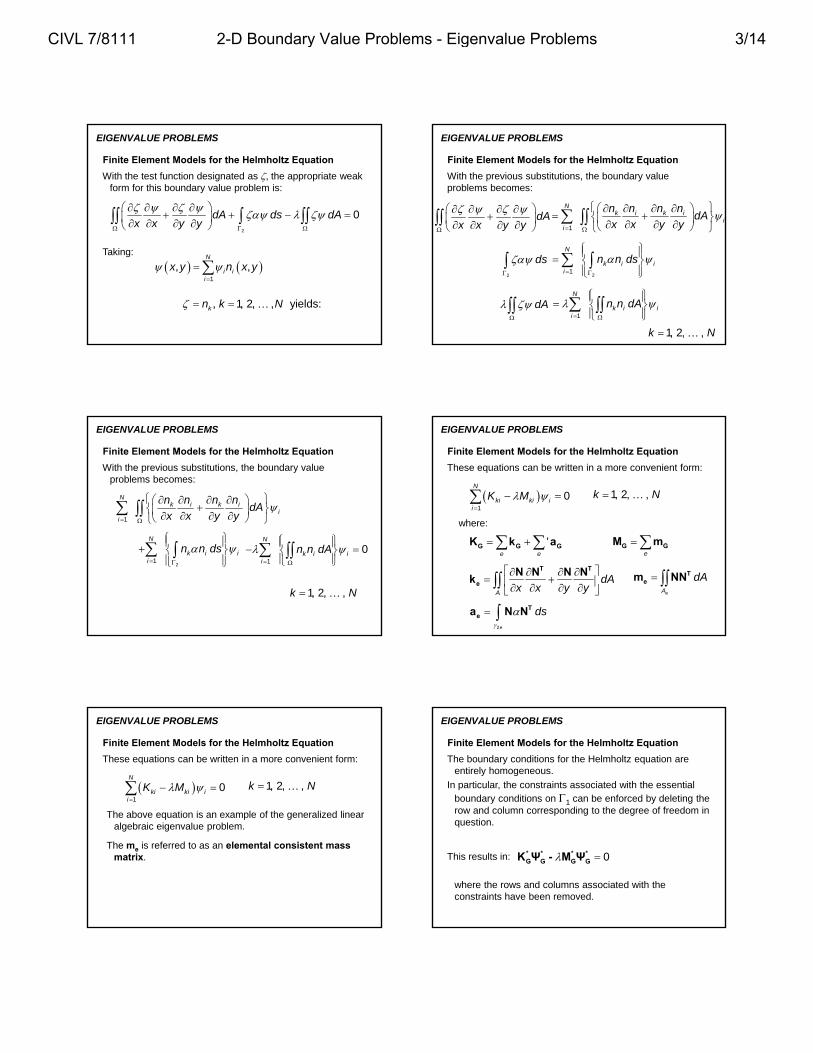
The first two eigenvectors clearly have a symmetric character in the 4 = 5 .

2

4

3

1

5

6

*1

0.643

0.643

1.0002

4

3

1

5

6

*2

0.250

0.250

1.000


EIGENVALUE PROBLEMS

One would suspect that these eigenvalues-eigenfunction pairs correspond to radially symmetric modes for the circle, with the lowest eigenvalue for this model representing an improvement in the single eigenvalue obtained from the first model using eight elements.

The third eigenvalue-eigenfunction demonstrates asymmetry with respect to the bisector of the angle subtended by the element.

2

4

3

1

5

6

*3

1.000

1.000

0.000


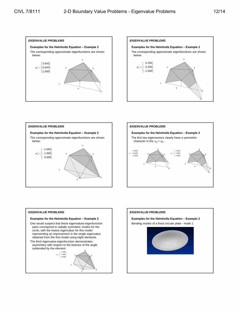
EIGENVALUE PROBLEMS

Bending modes of a fixed circular plate - mode 1



EIGENVALUE PROBLEMS

Bending modes of a fixed circular plate – mode 2


EIGENVALUE PROBLEMS



EIGENVALUE PROBLEMS



EIGENVALUE PROBLEMS

Normal vibration modes of a circular membrane


EIGENVALUE PROBLEMS



EIGENVALUE PROBLEMS



PROBLEM #26 - Consider the problem of a classical square vibrating membrane with all edges fixed against transverse displacement. The differential equation of motion can be written as:

EIGENVALUE PROBLEMS

22

2

wT w

t


210 in with 0 on

where T is the initial tension in the membrane and the area density. The boundary condition is that w vanishes on all the edges of the membrane. Taking:

where = 2/T

PROBLEM #26 - Model the top right-most quadrant of the membrane using eight equally-sized 3-node triangles and compute the associated eigenvalues and the eigenfunctions.

EIGENVALUE PROBLEMS

y

x

a

a

Note: Use a node numbering scheme that will make assembly of the stiffness and mass matrices as simple as possible.

End of

2-D Eigenvalues


chapter03g - eigenvalue problems · above equation are known as eigenvalues and eigenfunctions...

Documents

Transcript of chapter03g - eigenvalue problems · above equation are known as eigenvalues and eigenfunctions...