CHAPTER NUMBER DYNAMIC RAMP CONTROL STRATEGIES FOR RISK AVERSE SYSTEM OPTIMAL...

Dynamic Ramp Control Strategies for Risk Averse System Optimal Assignment 1

CHAPTER NUMBER

DYNAMIC RAMP CONTROL STRATEGIES FOR RISK AVERSE SYSTEM OPTIMAL ASSIGNMENT

Takashi Akamatsu, Graduate School of Information Sciences, Tohoku University, Sendai, Miyagi, Japan

Takeshi Nagae, Graduate School of Science and Technology, Kobe University, Kobe, Hyogo, Japan

INTRODUCTION

This paper explores dynamic ramp control strategies for a simple transportation network with stochastic travel time. The objective of the ramp metering considered here is not only to mitigate congestion in a freeway but also to achieve Dynamic System Optimal (DSO) assignment in a network with two parallel links; one of the links is a freeway with a single bottleneck, and the other is a local bypass link that can be regarded as an aggregation of a local street network. Travel time on the bypass link is assumed to follow a stochastic process due to many factors that cannot be controlled or predicted. A road network manager is expected to control the inflow rate to the freeway at each time point so as to attain the DSO assignment for a certain time horizon. We approach this problem by formulating it as a stochastic control problem (SCP), and then provide feedback (‘state contingent’) control rules that exploit the real-time observation of the realization of the stochastic state variable (i.e. random travel times). We then find that the optimal control (ramp metering) strategies at each time period can be classified into seven patterns, depending on the realization of the queue length in the freeway and the observed travel time of the bypass link. In order to obtain more detailed properties of the optimal control strategies, we need to solve the problem numerically. For this purpose, we reveal that the optimality conditions of the problem (i.e. Hamilton-Jacobi-Bellman (HJB) equations) can be equivalently

2 Insert book title here

2

stated as a dynamical system of Generalized Complementarity Problems (GCP). Based on this reformulation, we provide an efficient and robust algorithm for obtaining quantitative results for the control problem. Furthermore, we present results from systematic numerical experiments, which reveal how the uncertainty in the travel time affects the optimal control policies. Although there have been some studies on the DSO assignment in recent years, conventional approaches cannot be used to tackle the DSO assignment problem in this paper. Indeed, as we show below, little is known about the theoretical properties of the DSO assignment problem in deterministic models as well as stochastic environments in this paper. Friesz et al.(1989) study DSO assignment on a network with general topology. They present a deterministic optimal control formulation of the DSO assignment model, in which an ‘exit function’ is assumed for describing an outflow rate of a link. However, this modeling approach has the serious drawback of violating First-In-First-Out (FIFO) conditions according to which the traffic flow should be satisfied in each link. Ziliaskopoulous (2000) provides a linear programming (LP) formulation of the DSO assignment on a network with a one-to-many OD pattern, in which the cell transmission model (CTM) of Daganzo (1994) is employed to describe traffic flow propagation. However, in order for the LP formulation to be consistent with the CTM, we have to assume that the position of any vehicle can always be controlled (eg. stopped; the assumption of ‘holding’). This is a problematic assumption to implement, and hence it is questionable to think that this model represents a natural DSO assignment. We should also note that analysis for general networks might face difficulties due to the non-convexity of the DSO assignment problem even if we could provide a sound model of the DSO assignment preserving FIFO conditions (for this point, see Lovel and Daganzo (2000) and Erera et al.(2002)). In view of these studies, it seems that analyzing the model for general networks in one leap is not a very fruitful way to understand the theoretical properties of the DSO assignment. More recently, Kuwahara et al.(2000) and Munoz and Laval (2006) study the properties of the optimal control (ramp metering) in simple parallel-link networks. They show a graphical solution method based on the concept of dynamic marginal cost, which provides useful insights into the DSO assignment. However, this method cannot be extended systematically to the DSO assignment problem with stochastic travel time. Thus, our novel approach based on stochastic control theory as well as the theoretical findings contribute to the studies on dynamic traffic assignment and control. This paper is organized as follows: After presenting the stochastic control formulation of our DSO assignment model in the next section, we derive the HJB equations of the SCP in the third section. We then show some qualitative properties of the optimal control policies. In the fourth section, we reformulate the HJB equations for the DSO assignment as a system of GCPs, which enables us to develop an efficient solution method for the DSO assignment. In the fifth section, we provide an illustrative example of the proposed control method. The final section summarizes the paper.


DYNAMIC SYSTEM OPTIMAL RAMP METERING UNDER UNCERTAINTY

Networks and Link Models

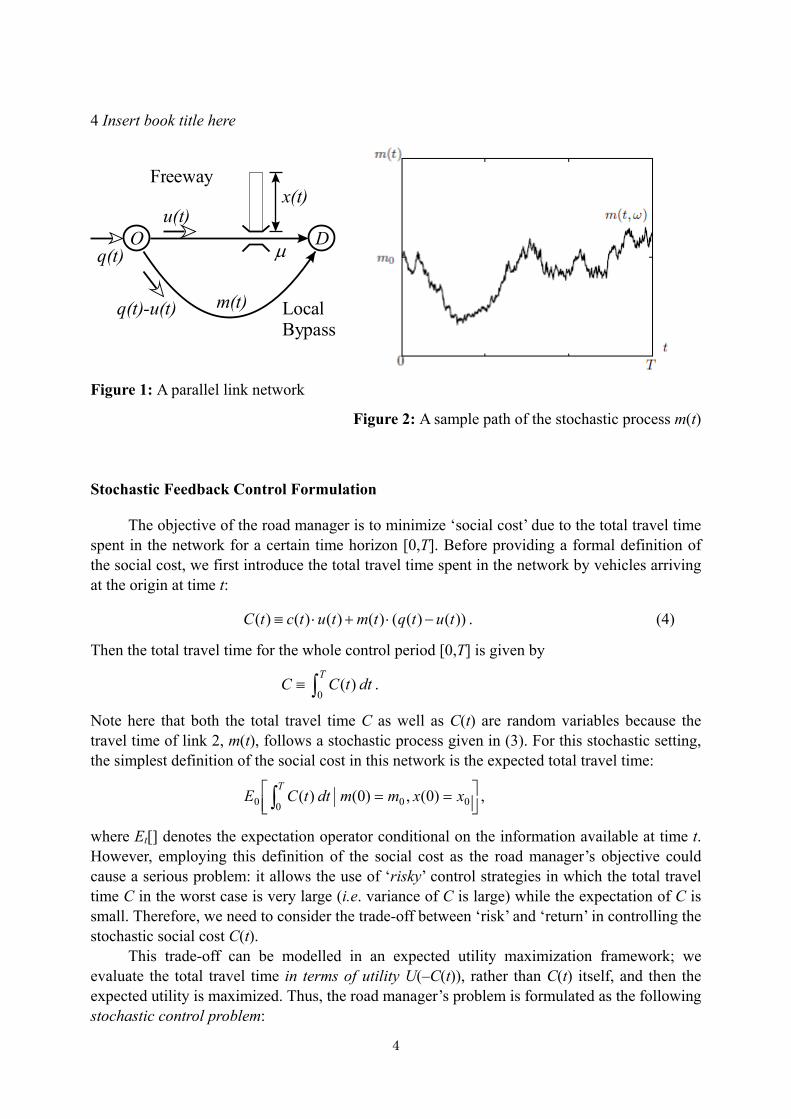
We consider a dynamic system optimal (DSO) assignment problem defined on a simple network with two parallel links connecting a single origin-destination (OD) pair (see Figure 1). One of the links, link 1, is a freeway with a single bottleneck of capacity μ , and the other, link 2, is a local bypass link with a very large capacity; link 2 may be regarded as a virtual link that is an aggregation of a local street network. We suppose that the number of vehicles arriving at the origin of the network until time t, Q(t), is known for all t in a fixed time period [0,T]. In the DSO assignment, a road network manager is assumed to control the inflow rate to the freeway, u(t), at each time point t; this implicitly determines the inflow rate to link 2 as q(t) – u(t), where q(t) is the OD flow rate at time t defined as q(t) = dQ(t)/dt. Thus, the DSO assignment considered in this paper can be viewed as a ramp-metering problem with a single freeway on-ramp. We suppose that the travel time of link 1 at time t, c(t), is determined simply by the queue length, x(t), at the bottleneck:

μ/)()( txtc = , (1) and the queue evolution is governed by the following state equation (i.e. the point-queue model is assumed):

[ ]⎩⎨⎧

=−>−

=0)(if0,)(max0)(if)(

)(txtutxtu

txμ

μ& , 0)0( =x , (2)

where u(t) is the controlled inflow rate into link 1. The travel time of link 2, m(t), is supposed to be just a function of time, which implies that m(t) can not be controlled by a road manager’s metering strategies. We also assume that m(t) evolves unpredictably over time due to many factors (such as fluctuation of OD flows into the local street network or traffic accidents) that cannot be controlled or predicted. We model the stochastic dynamics of m(t) as

dWdtttmdm )()(/ σα += , m(0) = m0, (3)

where W(t) is a standard Wiener process; )(tα and σ are an exogenously given (time- dependent) function and a volatility parameter, respectively. To illustrate the intuitive meanings of (3), in Figure 2, we provide an example of a sample path of the stochastic process m(t).


4

μO D

x(t)

q(t)

m(t)

Freeway

LocalBypass

u(t)

q(t)-u(t)

Figure 1: A parallel link network

Figure 2: A sample path of the stochastic process m(t)

Stochastic Feedback Control Formulation

The objective of the road manager is to minimize ‘social cost’ due to the total travel time spent in the network for a certain time horizon [0,T]. Before providing a formal definition of the social cost, we first introduce the total travel time spent in the network by vehicles arriving at the origin at time t:

))()(()()()()( tutqtmtutctC −⋅+⋅≡ . (4)

Then the total travel time for the whole control period [0,T] is given by

∫≡T

dttCC

0 )( .

Note here that both the total travel time C as well as C(t) are random variables because the travel time of link 2, m(t), follows a stochastic process given in (3). For this stochastic setting, the simplest definition of the social cost in this network is the expected total travel time:

⎥⎦⎤

⎢⎣⎡ ==∫ 00

0 0 )0(,)0( )( xxmmdttCET

,

where Et[] denotes the expectation operator conditional on the information available at time t. However, employing this definition of the social cost as the road manager’s objective could cause a serious problem: it allows the use of ‘risky’ control strategies in which the total travel time C in the worst case is very large (i.e. variance of C is large) while the expectation of C is small. Therefore, we need to consider the trade-off between ‘risk’ and ‘return’ in controlling the stochastic social cost C(t). This trade-off can be modelled in an expected utility maximization framework; we evaluate the total travel time in terms of utility U(–C(t)), rather than C(t) itself, and then the expected utility is maximized. Thus, the road manager’s problem is formulated as the following stochastic control problem:


[SCP] { }

( ) ⎥⎦

⎤⎢⎣

⎡==−−∫≤≤

00

2

0 0)()(0

)0( ,)0( 2

)()(max xxmmTxdCUET

tqtu μττ (5)

subject to eqs.(2) and (3); and )(Tx is free.

A few remarks are in order here: first, the problem formulated above, [SCP], is not an open-loop control problem, in which {u(t)} is determined in advance before controlling and observing the realization of state variables {x(t)} and {m(t)}; rather the problem [SCP] gives a feedback (‘state contingent’) control, in which the optimal inflow rate u(t) is a function of state variables, x(t) and m(t), observed at time t. This implies that the optimal control for [SCP] exploits the real-time observation of the realization of the stochastic state variable (i.e. random travel time m(t)). Second, the optimal control depends on a degree of risk aversion towards potentially ‘risky’ control strategies that exhibit a large variance of C; a risk averse manager should prefer a ramp control strategy that exhibits less risky control to a more risky one with the expectation of C being equal. The degree of risk aversion is reflected by a concave utility function U(–C) in our model; the higher the curvature of U(–C), the higher the risk aversion of the road manager.

OPTIMALITY CONDITIONS

Hamilton-Jacobi-Bellman Equations

We shall derive the optimality conditions for the SCP formulated in the previous section. We first define the value function V(t, x, m) by

{ }

( ) ⎥⎦⎤

⎢⎣⎡ ==−≡ ∫

T

tttumtmxtxdCUEmxtV

)()( ,)( )(max),,( ττ . (6)

By applying the dynamic programming (DP) principle, we have

⎥⎦⎤

⎢⎣⎡ ==Δ++−= ∫

Δ+mtmxtxmxtVmxtVdCUEmxtV

t

tttu)( ,)( ),,(),,())(( max),,(

)(ττ ,

where ∫Δ+

≡Δt

tddVmxtV

)( ),,( ττ . Taking the limit of 0+→Δ and using stochastic calculus

(Ito’s lemma):

22

2 )(

21

dm

mVdm

mVdx

xVdt

tVdV

∂∂

+∂∂

+∂∂

+∂∂

= , (7)

we obtain the Hamilton-Jacobi-Bellman (HJB) equation:


6

+⎥⎦⎤

⎢⎣⎡

∂∂

+−=≤≤ x

VtuxtCUtqtu

))(())((.max0 )()(0

&2

222

)(

21)()(

mVtm

mVtmt

tV

∂∂

+∂∂

+∂∂ σα

for all ),0[ Tt∈ . (8)

In order to avoid notational complexity, we denote this in a more compact form as

VLtuZtqtu

0)()(0))((.max0 +=

≤≤ for all ),0[ Tt∈ , (9)

with an infinitesimal generator L0 defined as

2

222

0

)(21)()(

mtm

mtmt

tL

∂∂

+∂∂

+∂∂

≡ σα , (10)

and the term Z(u(t)) involving the control variable u(t):

xVtuxtuCUtuZ

))(()))((())((∂∂

+−≡ &

⎩⎨⎧

=−+−>−+−

=0)( ]0 ,)(.[max)))(((

0)( ))(()))(((txifVtutuCUtxifVtutuCU

x

x

μμ

, (11)

where the subscript of V denotes the partial derivative (i.e. xVVx ∂∂≡ / ).

Optimal Control Strategies

Optimal control can be derived by solving the maximization problem (with respect to u(t)) in the HJB equation (9). Since the objective function Z takes two distinct forms depending on whether 0)( =tx or 0)( >tx , we will divide the derivation into two cases.

(a) The case of x(t) = 0

When there is no queue in the freeway, the function Z(u) should be further classified into two cases due to the indifferentiability of the max. function in the state equation (2). For the first case in which 0]0 ,)(.[max =− μtu (i.e. μ<)(tu ), the derivative of Z is always positive:

0)())(())(,(0

>⋅−′≡=

∂∂ tmuCUtmuf

uZ , (12)

It follows from this that the optimal control in this case is to assign all the OD flow into the freeway:

control A: μ<== )( 0)( )()( tqandtxiftqtu . (13)

Substituting this into (9), we obtain the HJB equation for this case as VLC 000 += where


)0(0 UC ≡ . For the second case in which μμ −=− )(]0 ,)(.[max tutu (i.e. μ≥)(tu ), the optimality condition for a regular interior maximum to (9) is given by

),0,(),(0 0

mtVmufuZ

x+==∂∂ . (14)

Defining the inverse function of )(' ⋅U by )(⋅I , we can represent (14) as

)())(/),0,(( uCtmmtVI x −= .

Since )())(()( tmutquC ⋅−= for x(t) = 0, we obtain the interior solution u(t) = v0 as

⎟⎟⎠

⎞⎜⎜⎝

⎛+=

)())(,0,(

)(1)(0 tm

tmtVItm

tqv x . (15)

It can be proved that the solution v0 given by (15) is a monotone function of m(t), and there exist m* and m** such that

⎪⎪⎩

⎪⎪⎨

⎧

≤≥

<≤<≤

<<

)( )(

)( )(

)(

**0

***0

*0

tmmfortqv

mtmmfortqv

mtmforv

μ

μ

(16)

holds. Since the inflow rate u(t) is restricted by )()( tqtu ≤≤μ , (16) implies that the optimal control strategies for the case of 0)( =tx and μ≥)(tq are given by

⎪⎪⎩

⎪⎪⎨

⎧

≤=

<≤=

<=

)( )()(:

)( )(:

)( )(:

**

***0

*

tmmiftqtucontrol

mtmmifvtucontrol

mtmiftucontrol

D

C

B μ

. (17)

For these controls, the HJB equations that the value function V should satisfy can be obtained by substituting (17) into (9):

001 =+ VLC for control B,

00 =VN for control C, (18)

010 =+ VLC for control D,

where ( )))(()(1 tqtmUC −⋅≡ μ , ( ) 01 )( Lx

tqL +∂∂

−≡ μ , VLxV

tmvVN 000 )

)(1( +

∂∂

−−≡ μ .

Note that quantitative determination of m* and m** requires the identification of the value function by solving the HJB equations.

(b) The case of x(t) > 0

When there is a queue in the freeway, the optimality condition for an interior maximum


8

to (9) is given by

),,(),,(0 1

mxtVmxufuZ

x+==∂∂ (19)

where the function f1(u, x, m) is defined by

)./)(()()( and )())(())(),(,(1 μtxtmtdtduCUtmtxuf −≡⋅−′≡

Representing (19) as )())(/),,(( uCtdmxtVI x −= and using )()()()( tqtmtduuC +⋅−= , we obtain the interior solution as

⎥⎦

⎤⎢⎣

⎡⎟⎟⎠

⎞⎜⎜⎝

⎛+=

)())(),(,()()(

)(1

1 tdtmtxtVItqtm

tdv x . (20)

For any fixed value of x(t) > 0, the solution v1 given by (20) is a monotone function of m(t), and there exist m and m such that

⎪⎩

⎪⎨

⎧

≤≥

<≤<≤

<<

)( )(

)( )(0

)( 0

1

1

1

tmmfortqv

mtmmfortqv

mtmforv

(21)

holds (for the proof, see Akamatsu and Yamazaki (2006)). This, together with the constraint )()(0 tqtu ≤≤ , implies that the optimal control for the case of x(t) > 0 can be characterized by

the following three strategies:

⎪⎩

⎪⎨

⎧

≤=

<≤=

<=

)( )()(: control

)( )(: control

)( 0)(: control

1

tmmiftqtu

mtmmifvtu

mtmiftu

G

F

E

. (22)

The corresponding HJB equations can be obtained by substituting these controls into (9):

022 =+ VLC for control E,

01 =VN for control F, (23)

013 =+ VLC for control G,

where ( ))()(2 tqtmUC ⋅−= , ( ))()/)((3 tqtxUC ⋅−= μ ,

02 Lx

L +∂∂

−≡ μ , VLxVv

xV

tdVN 011 )(

)(1

+∂∂

−+∂∂

−≡ μ .

Note that these boundaries, m and m , are functions of (t, x(t)); this implies that the optimal control at time t is selected from either one of the controls E, F, or G, depending on the realization of both state variables x(t) and m(t).


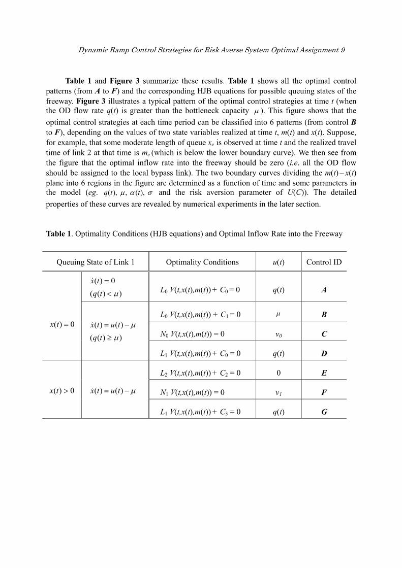
Table 1 and Figure 3 summarize these results. Table 1 shows all the optimal control patterns (from A to F) and the corresponding HJB equations for possible queuing states of the freeway. Figure 3 illustrates a typical pattern of the optimal control strategies at time t (when the OD flow rate q(t) is greater than the bottleneck capacity μ ). This figure shows that the optimal control strategies at each time period can be classified into 6 patterns (from control B to F), depending on the values of two state variables realized at time t, m(t) and x(t). Suppose, for example, that some moderate length of queue xe is observed at time t and the realized travel time of link 2 at that time is me (which is below the lower boundary curve). We then see from the figure that the optimal inflow rate into the freeway should be zero (i.e. all the OD flow should be assigned to the local bypass link). The two boundary curves dividing the m(t) – x(t) plane into 6 regions in the figure are determined as a function of time and some parameters in the model (eg. σαμ ),( , ),( ttq and the risk aversion parameter of U(C)). The detailed properties of these curves are revealed by numerical experiments in the later section.

Table 1. Optimality Conditions (HJB equations) and Optimal Inflow Rate into the Freeway

Queuing State of Link 1 Optimality Conditions u(t) Control ID

0)( =tx&

))(( μ<tq

L0 V(t,x(t),m(t)) + C0 = 0 q(t) A

L0 V(t,x(t),m(t)) + C1 = 0 μ B

N0 V(t,x(t),m(t)) = 0 v0 C

0)( =tx μ−= )()( tutx&

))(( μ≥tq

L1 V(t,x(t),m(t)) + C0 = 0 q(t) D

L2 V(t,x(t),m(t)) + C2 = 0 0 E

N1 V(t,x(t),m(t)) = 0 v1 F 0)( >tx μ−= )()( tutx&

L1 V(t,x(t),m(t)) + C3 = 0 q(t) G


10

Figure 3: The optimal control strategies at time t in the state space (m(t), x(t))

Comparisons with the Risk-neutral Strategies

It is worthwhile to discuss the optimal controls for the ‘risk neutral’ case in which the utility function is linear (i.e. the objective function of [SCP] reduces to only the expected total travel time). For the linear utility function, the objective function Z(u(t)) defined in (11) reduces to

⎩⎨⎧

=−+−>−+−

=0)( ]0 ,)(.[max))((

0)( ))(())(())((

txifVtutuCtxifVtutuC

tuZx

x

μμ

, (11’)

In a similar vein to the discussion of the previous subsection, the optimal control for this case may be divided according to whether the freeway queue exists or not (i.e. 0=x or 0≥x ). When x(t) = 0, the derivative of Z(u) is given by

⎩⎨⎧

≥+−<−

=∂∂

μμ

)( )(

tuifVmtuifm

uZ

x.

This implies that the function Z(u) is piecewise linear with respect to u, and the maximum is attained at either )()( tqtu = or μ=)(tu , depending on the sign of uZ / ∂∂ . Thus, the optimal metering strategy should be

⎩⎨⎧

≥=<=

),,()( )()(: ),,()( )(:

mxtVtmiftqtucontrolmxtVtmiftucontrol

x

x

DB μ

(17’)

Comparing this with the optimal control given in (17), we see that the control C vanishes in the risk-neutral case, and the control rule results in ‘bang-bang control’. When 0)( >tx , the derivative of Z(u) is given by


⎩⎨⎧

≥+−<−

=∂∂

μμμμ

)( )/( )( )/(

tuifVmxtuifmx

uZ

x.

This implies that the optimal control for this case is given by

⎩⎨⎧

+≥=+<=

),,()/( )( )()(: control ),,()/()( 0)(: control

mxtVxtmiftqtumxtVxtmiftu

x

x

μμ

GE

(22’)

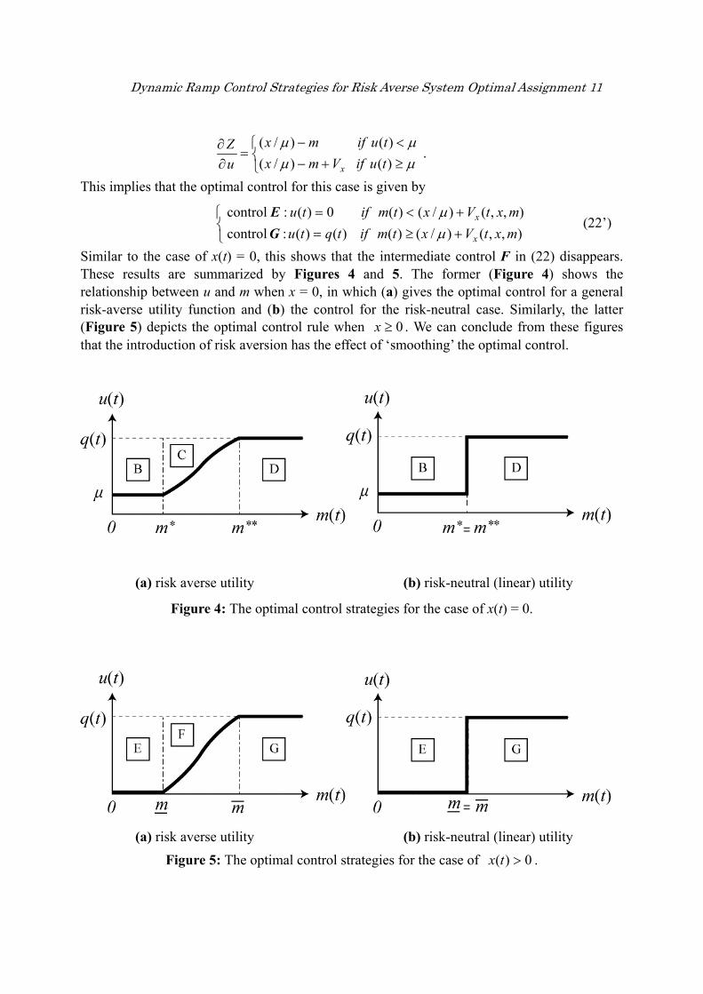
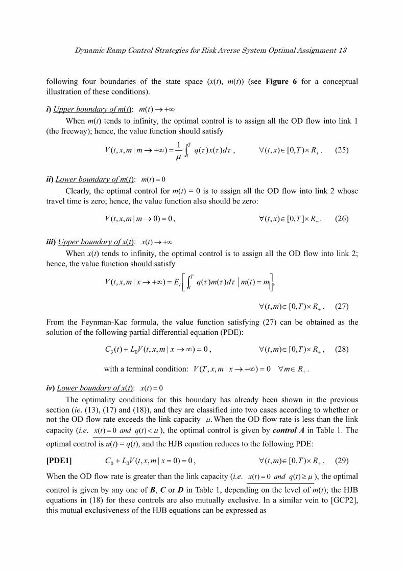
Similar to the case of x(t) = 0, this shows that the intermediate control F in (22) disappears. These results are summarized by Figures 4 and 5. The former (Figure 4) shows the relationship between u and m when x = 0, in which (a) gives the optimal control for a general risk-averse utility function and (b) the control for the risk-neutral case. Similarly, the latter (Figure 5) depicts the optimal control rule when 0≥x . We can conclude from these figures that the introduction of risk aversion has the effect of ‘smoothing’ the optimal control.

(a) risk averse utility (b) risk-neutral (linear) utility

Figure 4: The optimal control strategies for the case of x(t) = 0.

(a) risk averse utility (b) risk-neutral (linear) utility

Figure 5: The optimal control strategies for the case of 0)( >tx .


12

REFORMULATION AND NUMERICAL ALGORITHMS

In order to examine the detailed properties of the optimal control strategies (i.e. properties of v0, v1, and the two boundary curves in the state space), we need to solve the problem numerically. This section presents an efficient numerical algorithm for solving the SCP. For this purpose, we reveal that the optimality conditions of our problem (i.e. HJB equations) can be reformulated as a dynamical system of GCP. We then show that the system is decomposed with respect to time under an appropriate discretization framework. This enables us to reduce our problem to successively solving the sub-problems, each of which is formulated as a finite-dimensional GCP. We also provide an algorithm for solving the sub-problem. Due to space limitation, the technical details of the algorithm are relegated to Nagae and Akamatsu (2006a,b) and Akamatsu and Yamazaki (2006).

Reformulation as a Dynamical System of Nonlinear Complementarity Problems

(a) Optimality Conditions for the Inner Region

At any time ),0[ Tt ∈ in which x(t) > 0 holds, the optimal control is given by either E, F, or G (see Table 1). The HJB equations in (23) for these controls are also mutually exclusive. More concretely, suppose one of the controls, assume control E, is optimal at time t. Then, only one of the HJB equations in (23), C2+ L2V = 0 for control E, holds and the other HJB equations do not hold; it can be easily verified from the definition of the HJB equation (9) that 01 ≥VN and 013 ≥+ VLC when control E is optimal. This mutual exclusiveness of the HJB equations can be naturally expressed by the following dynamical system of GCP:

[GCP2] ⎩⎨⎧

≥+≥≥+=+⋅⋅+

0 ,0 ,0 0][][][

13122

13122

VLCVNVLCVLCVNVLC

++ ××∈∀ RRTmxt ),0[),,( (24a) or equivalently,

0)],,( ),,,( ),,,(.[min 12122 =++ mxtVLCmxtVNmxtVLC ,

++ ××∈∀ RRTmxt ),0[),,( (24b)

(b) Boundary Conditions

For [GCP2] to be a well-posed problem, the value function V(t) at any time t should satisfy some appropriate boundary conditions; we should consider the conditions on the


following four boundaries of the state space (x(t), m(t)) (see Figure 6 for a conceptual illustration of these conditions).

i) Upper boundary of m(t): +∞→)(tm When m(t) tends to infinity, the optimal control is to assign all the OD flow into link 1 (the freeway); hence, the value function should satisfy

∫=+∞→T

tdxqmmxtV

)()( 1)|,,( τττ

μ, +×∈∀ RTxt ),0[),( . (25)

ii) Lower boundary of m(t): 0)( =tm Clearly, the optimal control for m(t) = 0 is to assign all the OD flow into link 2 whose travel time is zero; hence, the value function also should be zero:

0)0|,,( =→mmxtV , +×∈∀ RTxt ],0[),( . (26)

iii) Upper boundary of x(t): +∞→)(tx When x(t) tends to infinity, the optimal control is to assign all the OD flow into link 2; hence, the value function should satisfy

,)( )()( )|,,(

⎥⎦⎤

⎢⎣⎡ ==+∞→ ∫ mtmdmqExmxtV

T

tt τττ

+×∈∀ RTmt ),0[),( . (27)

From the Feynman-Kac formula, the value function satisfying (27) can be obtained as the solution of the following partial differential equation (PDE):

0)|,,()( 03 =∞→+ xmxtVLtC , +×∈∀ RTmt ),0[),( , (28)

with a terminal condition: 0)|,,( =+∞→xmxTV +∈∀ Rm .

iv) Lower boundary of x(t): 0)( =tx The optimality conditions for this boundary has already been shown in the previous section (ie. (13), (17) and (18)), and they are classified into two cases according to whether or not the OD flow rate exceeds the link capacity .μ When the OD flow rate is less than the link capacity (i.e. μ<= )( 0)( tqandtx ), the optimal control is given by control A in Table 1. The

optimal control is u(t) = q(t), and the HJB equation reduces to the following PDE:

[PDE1] 0)0|,,(00 ==+ xmxtVLC , +×∈∀ RTmt ),0[),( . (29)

When the OD flow rate is greater than the link capacity (i.e. μ≥= )( 0)( tqandtx ), the optimal

control is given by any one of B, C or D in Table 1, depending on the level of m(t); the HJB equations in (18) for these controls are also mutually exclusive. In a similar vein to [GCP2], this mutual exclusiveness of the HJB equations can be expressed as


14

[GCP1] ⎩⎨⎧

≥+≥≥+=+⋅⋅+

0 ,0 ,0 0][][][

10001

10001

VLCVNVLCVLCVNVLC

+×∈∀ RTmt ),0[),( , (30a)

or equivalently, 0)],,( ),,,( ),,,(.[min 10001 =++ mxtVLCmxtVNmxtVLC ,

+×∈∀ RTmt ),0[),( . (30b) Finally, we should impose a terminal condition that must be satisfied by the value function at the terminal time T: 0),,( =mxTV ++ ×∈∀ RRmx ),( . (31) Thus, the SCP has been reformulated as a generalized complementarity problem [GCP], which consists of [GCP2] with four boundary conditions (i.e. eqs.(25), (26), (27), and [PDE1]/ [GCP1]) and a terminal condition (31).

Figure 6: The optimality conditions and four boundary conditions

that should hold at time t in the state space (m(t), x(t))

Discretization

In order to develop a numerical algorithm for solving [GCP], it is convenient to represent the problem in a discrete (time-state) framework. We consider a discrete grid in the time-state space ],0[],0[],0[ TMX ×× with increments dx, dm, and dt. Let (xi, mj, tk) be each point of the grid, where the indices i (= 0,1,..., I+1), j (= 0,1,..., J+1), and k (k = 0,1,…,K) characterize the locations of the point with respect to state variables x, m, and time t, respectively. We also denote the value of V(t, x, m) at a grid point (xi, mj, tk) by Vi,j(k). Using this grid point representation, we can approximate the value function V(t, x, m) at time tk by a (column) vector V(k) whose elements are [Vi, j(k) | i = 0,1,..., I+1; j = 0,1,..., J+1]. In this framework, infinitesimal operator Ln (n = 0,1,2) can be approximated as a matrix Ln by using an appropriate finite difference scheme (eg., that of Crank–Nicholson). Similarly,


infinitesimal operator Nn (n = 0 or 1) can be approximated by a set of nonlinear functions Nn of V(k). Thus, the three operators that appear in the HJB equations (23) for controls E, F, and G (i.e. VNVLC 122 ,+ , and VLC 13 + ) at time tk can be represented as

⎪⎩

⎪⎨

⎧

+−≡−≡

+−≡

++

+

++

)()()()1()1()(

)()1()(

)()()()1()1()(

311

11

222

)()(kkkkkk

kkk

kkkkkk

CVLVLGVNVNF

CVLVLE. (32)

We are now in a position to express [GCP] obtained in the previous subsection as a finite -dimensional GCP. To begin with, we represent the main problem [GCP2] (for time tk) by

[GCP2(k)] 0GFE =],,.[min )()()( kkk (33)

Next, the four boundary conditions from i) to iv) in 4.1 can be easily fitted into this discrete framework as follows. The first (original) boundary condition (for +∞→m ) is governed by (25) and the state equation (2). By using the discrete counterpart of (25):

∑=

+ Δ==K

kni

Ji txkxnxnqk ))(()(1)(V 1,

μ (34)

we easily obtain the values of {V i, J+1(k); i = 0,1,…,I }. The second condition (for m = 0) is given by (26), whose discrete correspondence is only to set

{V i, 0 (k) = 0; i = 0,1,…,I }. (35)

The third condition (for +∞→x ) is given by (27), which reduces to solving the PDE in (28). The discrete counterpart of this PDE is

0CA =+ )()( 3 kk , (36)

where A(k) is a discrete approximation of LoV, which is defined as

)()()1()1()( 00 kkkkk VLVLA −≡ ++ .

For given V(k+1), the system of linear equations (36) can be solved, which determines the value of {VI+1, j(k); j = 0,1,…, J }. The final boundary condition (for x = 0) is governed by [PDE1] and [GCP1]. The former reduces to the following system of linear equations:

[PDE1(k)] 0CA =+ )()( 0 kk , (37)

and the latter is represented by

[GCP1(k)] 0DCB =],,.[min )()()( kkk , (38)

where B(k), C(k) and D(k) are defined by

⎪⎩

⎪⎨

⎧

+−≡−≡

+−≡

++

+

++

)()()()1()1()(

)()1()(

)()()()1()1()(

011

00

100

)()(kkkkkk

kkk

kkkkkk

CVLVLDVNVNC

CVLVLB. (39)


16

The solution of (37)/(38) gives the value of V(k) on this boundary,{V0, j(k); j = 1,2,…, J }. In summary, [GCP] is thus expressed as a dynamical system of finite dimensional GCPs:

[GCP-D] 0GFE =],,.[min )()()( kkk for k = 0,1,…,K (40)

with the four boundary conditions:

i) {V i, J+1(k); i = 0,1,…,I } is given by (34), ii) {V i, 0 (k) = 0; i = 0,1,…,I }, iii) {V I+1, j(k); j = 0,1,…, J} is given by (36),

iv) ⎩⎨⎧

≥=<=μμ

)( ],,.[min)(

)()()(

)(

k

k

tqiftqif

kkk

k

0DCB0A

,

and a terminal condition: V(K) = 0.

Algorithm

The problem [GCP-D] has a convenient property that the sub-problem [GCP(k)] is independent from other sub-problems [GCP(l)] ( lk ≠ ) when V(k+1) is known. This implies that the series of sub-problems {[GCP(k)] | k = 0,1,...K} can be solved in a successive manner: using the terminal condition for V(K), we first solve the sub-problem [GCP(K–1)] and obtain the solution V(K–1); using V(K–1) as a given constant, we solve the sub-problem [GCP(K–2)] and obtain V(K–1); and by repeating the procedure recursively, we obtain the entire value function {V(k) | k = 0,1,2,…,K}. Since each sub-problem [GCP(k)] consists of [GCP2(k)] and the four boundary conditions, the procedure for obtaining V(k) is naturally divided into computation of V(k) on the boundaries and solving [GCP2(k)]. Thus, the outline of the algorithm for solving [GCP] can be summarized as follows:

Step 0. Set the terminal condition: 0V =:)(K ; Set time counter 1: −= Kk .

Step 1. Compute V(k) for the state space boundaries i) { V i, J+1(k); i = 0,1,…, I }, ii) { V i, 0 (k) = 0; i = 0,1,…,I }, and iii) { V I+1, j(k); j = 0,1,…, J }.

Step 2. Compute V(k) for the boundary iv) (i.e. {V0, j(k); j = 1,2,…, J}): Given V(k+1) and (V0, 0(k), V0, J+1(k)), solve [PDE1(k)] if μ≤)(kq , [GCP1(k)] otherwise.

Step 3. Compute V(k) for the inner region (i.e. {Vi, j(k); i = 1,2,…, I; j = 1,2,…, J }): Given V(k+1) and V(k) for all boundaries obtained in Step 1 and Step 2, solve [GCP2(k)].

Step 4. If k = 0 terminate, otherwise 1: −= kk and return to Step 1.

In the algorithm above, we need an efficient procedure for solving sub-problems [GCP1(k)] and [GCP2(k)], which are formulated as a finite-dimensional GCP. For this, we use a smoothing function approach developed by Peng (1998), Qi and Liao (1999), and Peng and


Lin (1999). This approach is not only the state-of-the-art technique but is also suitable for our problems with a special sparse Jacobian matrix from the view point of efficiency, as discussed in Akamatsu and Yamazaki (2006) and Nagae and Akamatsu (2006a,b). In the smoothing function approach, one solves the following system of nonlinear equations: 0VFVFVFVH =≡ )}(),(),(.{min)( 321 , (41)

where )}(),(),(.{min 321 VFVFVF is a vector operator whose j th element is defined as },,.{min 321

jjj FFF . Note that the equations system, H(V) = 0, cannot be solved by naive methods, since H(V) is indifferentiable. The key idea of the smoothing approach, in order to overcome difficulties due to the indifferentiability of H, is to transform the original problem into a system of smooth equations via a so-called smoothing function ),( ηVS with j th component,

]/)([expln ),( ηηη VV j

j

j FS −−≡ ∑ (42)

where 0≥η is referred to as the smoothing parameter. This type of function in eq.(42) is also known as an expected minimum cost (or a LOG-sum function) for a LOGIT model in the random utility theory. It is well known that the smoothing function has two desirable properties for developing an efficient algorithm: First,

)(),(lim)0,(0

VHVSVS =≡++→

ηη

.

In other words, the solution of the smooth equations system 0VS =),( η is equivalent to the solution of (41), H(V) = 0, at the limit of 0→η ; second, ),( ηVS is a continuously differentiable function of V for all 0>η . The former property ensures that the present algorithm provides a good approximation to the solution of (41), whereas the latter property is exploited to guarantee the efficiency of the algorithm. The smoothing approach-based algorithm generates a solution set of the smooth equations system, forming a path )}),( ,{( 0VSV =ηη as the parameter η tends to zero. This path is usually referred to as the smoothing path. Let )(nη denote the smoothing parameter in the n th iteration, and V(n) be a solution of the corresponding smooth equation 0VS =),( )(nη . For this notation, we can summarize the procedure for generating the smoothing path as

Step 0. Choose .)1(+∈Rη Set iteration counter 1:=n ;

Step 1. If 0VH =)( )(n terminate; V(n) is the solution of the GLCP; Step 2. Solve the smooth equations system 0VS =),( )()( nn η ; Step 3. Choose the next smoothing parameter ),0[ )()1( nn ηη ∈+ ; Step 4. Set 1: += nn ; return to Step 1.

It is easy to verify that any accumulation point of the smoothing path },{ )()( nn ηV generated by the algorithm above is the solution of (41), since the first property of the smoothing function

)()0,( VHVS =+ and the condition applicable to the smoothing parameters, 0)1()( ≥> +nn ηη is satisfied. The global convergence of the generic algorithm has been established (e.g. Peng and


18

Lin (1999)): Any smoothing path },{ )()( nn ηV generated by the algorithm converges to )0 ,( * +V globally, when i) ),( )()()( nnn ηVSS ∇≡∇ is nonsingular, and ii) the norm of 1)( ][ −∇ nS

is finite for all n. Since both the conditions are naturally satisfied in our framework, the smoothing path globally converges to the solution of (41).

ILLUSTRATIVE EXAMPLES OF CONTROL OPERATIONS

An Example Illustrating the Proposed Method

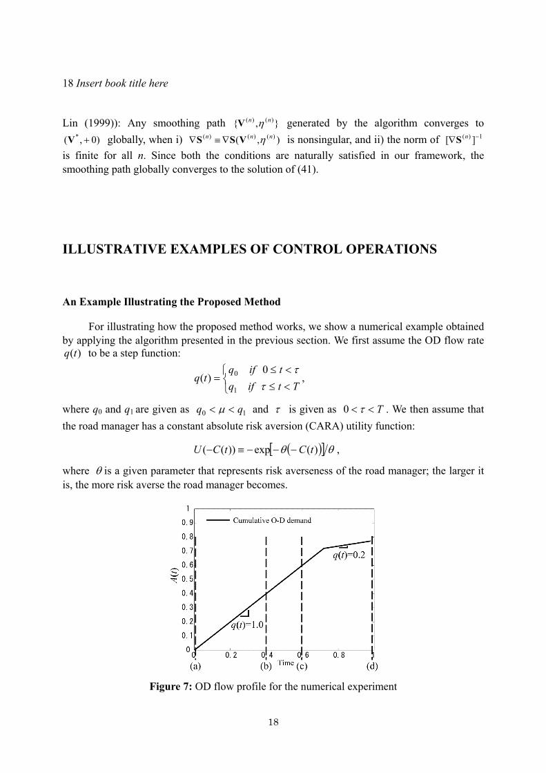
For illustrating how the proposed method works, we show a numerical example obtained by applying the algorithm presented in the previous section. We first assume the OD flow rate

)(tq to be a step function:

⎩⎨⎧

<≤<≤

=Ttifq

tifqtq

ττ

0

)(1

0 ,

where q0 and q1 are given as 10 qq << μ and τ is given as T<< τ0 . We then assume that the road manager has a constant absolute risk aversion (CARA) utility function:

( )[ ] θθ )(exp))(( tCtCU −−−≡− ,

where θ is a given parameter that represents risk averseness of the road manager; the larger it is, the more risk averse the road manager becomes.

Figure 7: OD flow profile for the numerical experiment


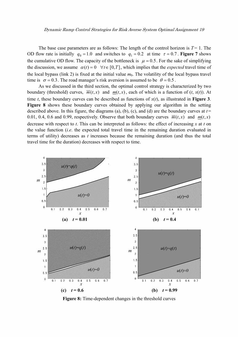
The base case parameters are as follows: The length of the control horizon is T = 1. The OD flow rate is initially 0.10 =q and switches to 2.01 =q at time 7.0=τ . Figure 7 shows the cumulative OD flow. The capacity of the bottleneck is 5.0=μ . For the sake of simplifying the discussion, we assume 0)( =tα ],0[ Tt∈∀ , which implies that the expected travel time of the local bypass (link 2) is fixed at the initial value m0. The volatility of the local bypass travel time is 3.0=σ . The road manager’s risk aversion is assumed to be 5.0=θ . As we discussed in the third section, the optimal control strategy is characterized by two boundary (threshold) curves, ),( xtm and ),( xtm , each of which is a function of (t, x(t)). At time t, these boundary curves can be described as functions of x(t), as illustrated in Figure 3. Figure 8 shows these boundary curves obtained by applying our algorithm in the setting described above. In this figure, the diagrams (a), (b), (c), and (d) are the boundary curves at t =

0.01, 0.4, 0.6 and 0.99, respectively. Observe that both boundary curves ),( xtm and ),( xtm decrease with respect to t. This can be interpreted as follows: the effect of increasing x at t on the value function (i.e. the expected total travel time in the remaining duration evaluated in terms of utility) decreases as t increases because the remaining duration (and thus the total travel time for the duration) decreases with respect to time.

(a) t = 0.01 (b) t = 0.4

(c) t = 0.6 (b) t = 0.99

Figure 8: Time-dependent changes in the threshold curves


20

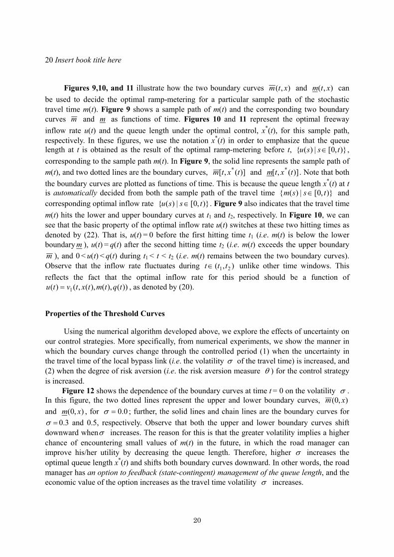
Figures 9,10, and 11 illustrate how the two boundary curves ),( xtm and ),( xtm can be used to decide the optimal ramp-metering for a particular sample path of the stochastic travel time m(t). Figure 9 shows a sample path of m(t) and the corresponding two boundary curves m and m as functions of time. Figures 10 and 11 represent the optimal freeway inflow rate u(t) and the queue length under the optimal control, x*(t), for this sample path, respectively. In these figures, we use the notation x*(t) in order to emphasize that the queue length at t is obtained as the result of the optimal ramp-metering before t, )},0[|)({ tssu ∈ , corresponding to the sample path m(t). In Figure 9, the solid line represents the sample path of m(t), and two dotted lines are the boundary curves, )](,[ * txtm and )](,[ * txtm . Note that both the boundary curves are plotted as functions of time. This is because the queue length x*(t) at t is automatically decided from both the sample path of the travel time )},0[|)({ tssm ∈ and corresponding optimal inflow rate )},0[|)({ tssu ∈ . Figure 9 also indicates that the travel time m(t) hits the lower and upper boundary curves at t1 and t2, respectively. In Figure 10, we can see that the basic property of the optimal inflow rate u(t) switches at these two hitting times as denoted by (22). That is, u(t) = 0 before the first hitting time t1 (i.e. m(t) is below the lower boundary m ), u(t) = q(t) after the second hitting time t2 (i.e. m(t) exceeds the upper boundary m ), and 0 < u(t) < q(t) during t1 < t < t2 (i.e. m(t) remains between the two boundary curves). Observe that the inflow rate fluctuates during ),( 21 ttt∈ unlike other time windows. This reflects the fact that the optimal inflow rate for this period should be a function of

))(),(),(,()( 1 tqtmtxtvtu = , as denoted by (20).

Properties of the Threshold Curves

Using the numerical algorithm developed above, we explore the effects of uncertainty on our control strategies. More specifically, from numerical experiments, we show the manner in which the boundary curves change through the controlled period (1) when the uncertainty in the travel time of the local bypass link (i.e. the volatility σ of the travel time) is increased, and (2) when the degree of risk aversion (i.e. the risk aversion measure θ ) for the control strategy is increased. Figure 12 shows the dependence of the boundary curves at time t = 0 on the volatility σ . In this figure, the two dotted lines represent the upper and lower boundary curves, ),0( xm and ),0( xm , for 0.0=σ ; further, the solid lines and chain lines are the boundary curves for =σ 0.3 and 0.5, respectively. Observe that both the upper and lower boundary curves shift

downward whenσ increases. The reason for this is that the greater volatility implies a higher chance of encountering small values of m(t) in the future, in which the road manager can improve his/her utility by decreasing the queue length. Therefore, higher σ increases the optimal queue length x*(t) and shifts both boundary curves downward. In other words, the road manager has an option to feedback (state-contingent) management of the queue length, and the economic value of the option increases as the travel time volatility σ increases.


Figure 9: A sample path of m(t) and the corresponding threshold curves

for the control period [0,1]

Figure 10: Optimal inflow rate for the sample path of m(t) in Figure 9.

Figure 11: Queue evolution in the freeway for the optimal metering in Figure 10.


22

Figure 13 shows the way in which the boundary curves change with respect to the road manager’s risk averseness, θ . In this figure, each pair of solid lines, dotted lines, and chain lines represents the boundary curves at t = 0 for =θ 0.1, 0.3, and 0.9, respectively. We can see that the upper boundary curve increases with respect to θ , whereas the lower boundary curve decreases. This implies that when the manager is more risk averse, an extreme control, i.e. either u(t) = 0 or u(t) = q(t), becomes not optimal.

Figure 12: The threshold curves for various levels of volatility

Figure 13: The threshold curves for various levels of risk-aversion


CONCLUDING REMARKS

This paper provides ramp control strategies that achieve dynamic system optimal assignment on a network with two parallel links; one of the links is a freeway with a single bottleneck, and the other is a local bypass link (or an aggregation of a local street network) whose travel time follows a stochastic process. Formulating the model as a continuous-time stochastic control problem, we provide feedback (‘state contingent’) control rules that exploit the real-time observation of the realization of the stochastic travel time. Our theoretical analysis shows that the optimal ramp control strategies at each time period can be classified into seven patterns (as summarized in Table 1 and Figure 3), depending on the realization of queue length in the freeway and the observed travel time of the bypass link. We further reveal that the optimality conditions of the problem can be reformulated as a dynamical system of generalized complementarity problems, which enables us to provide an efficient and robust algorithm for obtaining quantitative results for the control problem. Finally, we provide an illustrative example of the proposed control method, and present results from systematic numerical experiments, which reveal how the uncertainty in travel time affects the optimal control policies.

ACKNOWLEDGMENT

The authors are grateful to Shuichi Yamazaki for his significant assistance in the numerical experiments presented in this paper.

REFERENCES

Akamatsu, T. and S. Yamazaki (2006). An efficient algorithm for risk averse dynamic system optimal traffic assignment. Infrastructure Planning Review, 23, 963-972.

Cottle, R. W., and G. B. Dantzig (1970). A generalization of the linear complementarity problem. Journal of Combinatorial Theory, 8, 79–90.

Erera, A.L., C.F. Daganzo, and D.J. Lovell (2002). Access control problem on capacitated FIFO networks with unique origin-destination paths is hard. Operations Research, 50, 736-743.

Ferris, M.C., and J.-S. Pang (1997). Engineering and economic applications of complemen -tarity problems. SIAM Review, 39, 669–713.

Friesz, T.L., J. Luque, R. Tobin and B. Wie (1989). Dynamic network traffic assignment considered as a continuous time optimal control problem. Operations Research, 37，893-901.

Kuwahara, M., T. Yoshii and K. Kumagai (2001). An analysis on dynamic system optimal assignment and ramp control on a simple network. JSCE Journal of Infrastructure Planning and Management, 667/IV-50，59-71.

Lovell, D.J. and C.F. Daganzo (2000). Access control on networks with unique origin- destination paths. Transportation Research, 34B, 185-202.


24

Munoz, J.C. and J.A. Laval (2006). System optimal dynamic traffic assignment graphical solution method for a congested freeway and one destination. Transportation Research, 40B, 1-15.

Nagae, T. and T. Akamatsu (2006a). A generalized complementarity approach to solving real option problems. Journal of Economic Dynamics and Control (in press).

Nagae, T. and T. Akamatsu (2006b). Dynamic system optimal traffic assignment exploiting information on real-time traffic conditions. JSCE Journal of Infrastructure Planning and Management (in press).

Peng, J.-M. (1999). A smoothing function and its applications, in: M. Fukushima and Qi Liqun (Eds.), Reformulation: Nonsmooth, Piecewise Smooth, Semismooth and Smoothing Methods. Kluwer Academic Publishers, 293–316.

Peng, J.-M., and Z. Lin (1999). A non-interior continuation method for generalized linear complementarity problem. Mathematical Programming, 86, 533-563.

Qi, H.-D. and L.-Z. Liao (1999). A smoothing Newton method for extended vertical linear complementarity problem. SIAM Journal on Matrix Analysis and Applications, 21, 45-66.

Ziliaskopoulos, A.K. (2000). A linear programming model for the single destination system optimum dynamic traffic assignment problem. Transportation Science, 34, 1-12.

CHAPTER NUMBER DYNAMIC RAMP CONTROL STRATEGIES FOR RISK AVERSE SYSTEM OPTIMAL...

Documents

Transcript of CHAPTER NUMBER DYNAMIC RAMP CONTROL STRATEGIES FOR RISK AVERSE SYSTEM OPTIMAL...